Rethinking the design of infiltration facilities
64
Transcript of Rethinking the design of infiltration facilities

II
Rethinking the design of infiltration facilities
Master of Science Thesis
15 May 2009
Leon Adrianus Valkenburg
1170546
Delft University of Technology
Faculty of Geosciences and Civil Engineering
Department of Watermanagement
Section of Water Resources Management
Graduation committee:
Prof.dr.ir. N.C. van de Giesen - TU Delft Water Resources Management
Dr.ir. F.H.M. van de Ven - TU Delft/Deltares
Water Resources Management
Ir. J.A.E. ten Veldhuis - TU Delft Urban Drainage
Ir. E.C. Hartman – DHV
Urban Watermanagement

III
Preface This thesis has been written as the final step towards a Master of Science degree in Watermanagement at the Civil Engineering faculty of the TU Delft. During an MSc research the student has to show his capabilities after 5 years of study in the form of a scientific research. In my case I have done research on the design of infiltration facilities. When I started the research I only had a simple idea about infiltration facilities. So at the start it was somewhat like opening a door to a whole new aspect of water management. And somehow you have to show yourself the way. As I found out during the months, there is a lot to be discovered about infiltration facilities. The unsaturated zone, the part of the soil in which the infiltration facilities are constructed, is one of the most complex and least studied parts of the hydrological system. Infiltration facilities themselves are also hardly studied as well. Doing research on infiltration facilities sometimes felt like pioneering. Basically, the current design method for infiltration facilities is scientifically wrong. This generally leads to facilities which much better than expected during the design. It proved to be challenging to come up with improvements to the design method, which are both scientifically acceptable and applicable in practice. I hope this research is a step towards a better design of infiltration facilities. So enjoy reading and if you have any questions, do not hesitate to contact me! Leon Valkenburg May the 15th, 2009

IV
Acknowledgements Fortunately I couldn’t have finished my study and written this thesis all by myself. It is a good thing you can always depend and rely on people close to you. Actually, if I would have written my thesis on my own, it would probably have been very boring and bad piece of work. Now I think it has become a really nice piece of work, not only because of my own efforts, but also thanks to the help of many, many people. So thank you all!! Some of you I want to mention in particular: First of all I would like to thank my main supervisors, Emil Hartman at DHV and Frans van de Ven at the TU Delft. Without their criticism and support I would probably still be wondering what to do. The DHV department of Mens, Stad and Water was of great help in facilitating my research. Also thanks go out to the other members of my committee, prof. Nick van de Giesen and Marie Claire ten Veldhuis. Also I want to thank the people from the municipality of Ede and Deltares Utrecht for helping me to do experiments with (their) infiltration facilities. Probably you don’t get requests from a student every day to go into the field and fill an infiltration facility, drill some holes in and next to it, add some measuring equipment and then see what happens. I think it was fun and it did deliver interesting results! Of course my friends and fellow MSc students were of great help. Writing a thesis can be tough, but doing it together makes it more fun. I will definitely remember the sometimes pretty odd, but usually nice lunch break discussions we had. Last, but not least, many thanks go out to my family. Without their help I would not have been able to complete my study. I hope I have made you proud!

V
Executive summary Currently urban sewer systems are facing two problems: pluvial flooding and combined sewer overflows (CSO). Both problems occur when the systems are overloaded due to heavy rainfall. Sustainable urban drainage systems (SUDS) have been developed to reduce the load on the drainage systems. Infiltration facilities are used as SUDS more and more. Basically an infiltration facility collects the storm water at the source (for instance at a parking lot) and lets the water soak into the soil. This research is focussed on the design of infiltration facilities. The functioning of infiltration facilities is affected by three main processes:
• Urban runoff: the amount of runoff water which can be expected to enter the facility. • Infiltration capacity of the facility: the flux of water which leaves the facility and enters the soil. • Clogging of the facility: during its lifetime the facility’s infiltration capacity is reduced by clogging of the surrounding soil and components of the facility itself. Clogging is the most important threat for the life expectancy of a facility.
In the design all three processes should be taken into account as accurate as possible. During this research four design methods for infiltration facilities have been analysed. The design guidelines from the UK, Germany, Australia and the Netherlands have been compared. The guidelines have similar approaches for the design of infiltration facilities. The design methods are all based on a calculation of the storage and dimensions of the designed facility given an inflow (urban runoff) and an infiltration capacity. However the basis of the design methods in all guidelines proved to be scientifically wrong. Several uncertainties have been identified on each of the three processes affecting the performance of the facilities. The biggest uncertainties (and assumptions) have been identified in the calculation of the infiltration capacity. These uncertainties have been investigated further. The assumptions and uncertainties in the calculation of the infiltration capacity were studied in two ways:
1. By modelling infiltration facilities in Hydrus 2D. The modelling with Hydrus showed that the current design methods underestimate the maximum infiltration capacity of facilities up to 30 times and overestimate the emptying time up to 15 times.
2. By measuring in existing infiltration facilities in the municipality of Ede. The measurements in two infiltration facilities in Ede showed that both facility still perform well years after construction. The old facility (from 1980) was empty within half a day. The “new” facility (from 2001) infiltrated the water faster than the water could be discharged to the facility. In both facilities the bottom proved not be clogged.
The design has been refined based on the model results and the measurements in infiltration facilities. The main change was the introduction of a refined infiltration model:
• The calculation of the hydraulic gradient dependent on the water level in the facility, the soil suction and a saturated zone around the facility.
• Taking into account the bottom area of the facility. • Considering the groundwater level in the design of a facility.
The refined infiltration model has simulated the results from the measurements and the modelling much better. Therefore the new design method should replace the current design method.

VI
Samenvatting Rioolsystemen hebben tegenwoordig te maken met twee problemen: wateroverlast en riooloverstorten. Beide problemen ontstaan wanneer de systemen overbelast zijn als gevolg van zware regenval. Om de belasting op de riolering te verminderen zijn afkoppelvoorzieningen ontwikkeld. Infiltratievoorzieningen worden steeds vaker gebruikt als afkoppelvoorziening. Een infiltratievoorziening verzamelt het water bij de bron (bijvoorbeeld bij een parkeerplaats) en laat het water de bodem in lopen. Dit onderzoek is gericht op het ontwerp van infiltratievoorzieningen. De werking van infiltratievoorzieningen wordt vooral beïnvloed door drie processen:
• Stedelijke afvoer: de hoeveelheid water die naar de voorziening stroomt. • Infiltratie capaciteit van de voorziening: het debiet dat vanuit de voorziening de bodem in loopt. • Dichtslibben van de voorziening: tijdens de levensduur van de voorziening vermindert de infiltratiecapaciteit door verstopping van de omringende bodem en delen van de voorziening zelf. Verstopping is de belangrijkste bedreiging voor de capaciteit van een voorziening.
Bij het ontwerp moet men zo goed mogelijk rekening houden met alle drie processen. Tijdens dit onderzoek zijn vier ontwerpmethoden voor infiltratievoorzieningen geanalyseerd. De ontwerprichtlijnen uit het Verenigd Koninkrijk, Duitsland, Australië en Nederland zijn vergeleken. De richtlijnen hebben vergelijkbare methoden voor het ontwerp van infiltratievoorzieningen. Ze zijn allemaal gebaseerd op een berekening van de berging en de afmetingen van een voorziening met een gegeven instroom (stedelijke afvoer) en een infiltratie capaciteit. De onderbouwing van de ontwerpmethode van de richtlijnen bleek wetenschappelijk onjuist te zijn. Verschillende onzekerheden zijn geïdentificeerd op elk van de drie processen die de werking van de voorzieningen beïnvloeden. De grootste onzekerheden (en aannames) bleken in de berekening van de infiltratiecapaciteit te zitten. Deze onzekerheden zijn verder onderzocht. De aannames en onzekerheden in de berekening van de infiltratiecapaciteit zijn op twee manieren bestudeerd:
1. Door modelleren van infiltratie voorzieningen in het onverzadigde zone model Hydrus 2D. Uit de resultaten van Hydrus bleek dat de huidige ontwerpmethoden de maximale infiltratie capaciteit van de installaties tot 30 keer onderschatten en de ledigingstijd tot 15 maal overschatten.
2. Door te meten in de bestaande voorzieningen in de gemeente Ede. Uit de metingen in twee infiltratievoorzieningen in Ede bleek dat deze voorzieningen (tientallen) jaren na aanleg nog goed infiltreerden. De oudere voorziening (uit 1980) was binnen een halve dag leeg. De jongere voorziening (uit 2001) infiltreerde sneller dan het water toegevoerd kon worden. De bodem bleek bij beide voorzieningen niet dichtgeslibd te zijn.
Op basis van het modelleren en meten van infiltratievoorzieningen is de ontwerpmethode verfijnd. De belangrijkste wijziging was de introductie van een verfijnd infiltratie model:
• De hydraulische gradiënt is afhankelijk van het waterniveau in de voorziening, de aanzuigende werking van de grond en een verzadigde zone rondom de voorziening.
• Het bodemoppervlak van de voorziening wordt meegerekend. • De grondwaterstand van een voorziening wordt meegenomen in het ontwerp.
Dit nieuwe infiltratiemodel benadert de model- en meetresultaten veel beter dan de oude en zou daarom de huidige ontwerpmethode moeten vervangen.
VII
Table of contents Preface ............................................................................................................................. III Acknowledgements .............................................................................................................IV Executive summary ..............................................................................................................V Samenvatting .....................................................................................................................VI Table of contents ...............................................................................................................VII List of figures...................................................................................................................... IX List of tables....................................................................................................................... IX 1. Introduction..................................................................................................................... 1
1.1 Urban drainage and infiltration facilities......................................................................... 1 1.2 Infiltration facilities...................................................................................................... 1 1.3 Scope of this research ................................................................................................. 3 1.4 Research question....................................................................................................... 3 1.5 Research method ........................................................................................................ 3 1.6 Readers guide............................................................................................................. 3
2. Processes influencing infiltration facilities............................................................................ 4
2.1 Urban runoff ............................................................................................................... 4 2.1.1 Rainfall................................................................................................................. 4 2.1.2 Runoff generation ................................................................................................. 5
2.2 The infiltration capacity................................................................................................ 6 2.2.1 Darcy’s description of groundwater flow .................................................................. 7 2.2.2 Deriving Richards’ equation.................................................................................... 7 2.2.3 Applying Richards’ equation ................................................................................... 8 2.2.4 Simplifications of Richards’ equation ....................................................................... 8 2.2.5 Temperature effect................................................................................................ 9
2.3 Clogging................................................................................................................... 10 2.3.1 The clogging process........................................................................................... 10 2.3.2 Quantifying clogging............................................................................................ 10
3. Current design practice................................................................................................... 11
3.1 The inflow ................................................................................................................ 11 3.2 Determining the infiltration capacity............................................................................ 12 3.3 Determining the dimensions and the storage ............................................................... 13
3.3.1 Emptying time .................................................................................................... 14 4. Studying the infiltration capacity...................................................................................... 15
4.1 Modelling infiltration facilities...................................................................................... 15 4.1.1 Model description ................................................................................................ 15 4.1.2 Setup of model ................................................................................................... 16 4.1.3 Results ............................................................................................................... 16
VIII
4.1.4 Conclusions ........................................................................................................ 20 4.2 Monitoring infiltration facilities .................................................................................... 21
4.2.1 Case study in Ede................................................................................................ 22 4.2.2 Location case study ............................................................................................. 22 4.2.3 The tested facilities ............................................................................................. 22 4.2.4 Setup of measurements ....................................................................................... 24 4.2.5 Results ............................................................................................................... 25 4.2.6 Conclusions ........................................................................................................ 28
5. Refining the design methodology..................................................................................... 29
5.1 Determining the inflow .............................................................................................. 29 5.2 Determining the infiltration capacity............................................................................ 29
5.2.1 The hydraulic conductivity.................................................................................... 30 5.2.3 The hydraulic gradient ......................................................................................... 30 5.2.4 The infiltrating area............................................................................................. 31
5.3 Determining the dimensions....................................................................................... 32 5.3.1 Emptying time .................................................................................................... 32
5.4 Testing the refined infiltration model........................................................................... 32 5.4.1 Groundwater level ............................................................................................... 33 5.4.2 Varying hydraulic conductivity .............................................................................. 33 5.4.3 Varying side-bottom ratio..................................................................................... 34 5.4.4 Varying clogged bottom ratio ............................................................................... 34 5.4.5 Measurements results.......................................................................................... 35 5.4.6 Design example .................................................................................................. 36
6. Conclusions & recommendations...................................................................................... 37
6.1 Conclusions .............................................................................................................. 37 6.2 Recommendations..................................................................................................... 37
References ........................................................................................................................ 39 Annexes ...............................................................................................................................ii
Annex I Hydrus modelling graphs...................................................................................... iii Annex II Measuring plan in Ede (in Dutch) ........................................................................ viii Annex III Contacted stakeholders.................................................................................... xiii
A. The 90 emailed municipalities* for monitoring data .................................................... xiii B. Interviewed stakeholders ......................................................................................... xiii

IX
List of figures Figure 1 Consequences of sewer overloading: pluvial flooding and CSO’s .................................. 1 Figure 2 An infiltration facility................................................................................................ 2 Figure 3 Types of infiltration facilities ..................................................................................... 2 Figure 4 pF curves for various soil types after Dreven, van et al (2000) .................................... 6 Figure 5 Plotting K, θ and ψm against the column length after Hillel (1971) ............................... 7 Figure 6 Green-Ampt schematisation of infiltration .................................................................. 9 Figure 7 Relation storage (S), infiltration capacity (q) and inflow (T=p year) after Monster & Leeflang (1996) ................................................................................................................. 14 Figure 8 The Hydrus 2D model: setup for maximum discharge and setup for emptying ............ 15 Figure 9 Influence groundwater level on discharge and emptying time ................................... 17 Figure 10 Influence hydraulic conductivity on discharge and emptying time ............................ 18 Figure 11 Influence facility's shape on discharge and emptying time....................................... 18 Figure 12 Influence clogged bottom on discharge and emptying time ..................................... 19 Figure 13 Influence initial moisture content on emptying time................................................ 20 Figure 14 Influence varying temperature on discharge and emptying time .............................. 20 Figure 15 Location of the tested facilities (Google Earth) ....................................................... 22 Figure 16 Studied infiltration facilities at the Horapark and the Buurtscheuterlaan in Ede.......... 23 Figure 17 Top view of sensor setup at the Buurtscheuterlaan................................................. 24 Figure 18 Fieldwork at the Horapark (on the left) and the Buurtscheuterlaan in Ede................. 25 Figure 19 Water level measurements in the Horapark soakaway............................................. 25 Figure 20 Q-h relation for Horapark soakaway ...................................................................... 26 Figure 21 Soil moisture measurements at the Buurtscheuterlaan ............................................ 27 Figure 22 Schematisation of 2D infiltration ........................................................................... 31 Figure 23 Comparing design methods for varying groundwater level....................................... 33 Figure 24 Comparing design methods for varying hydraulic conductivity ................................. 33 Figure 25 Comparing design methods for varying side-bottom ratio........................................ 34 Figure 26 Comparing design methods for varying clogged bottom ratio................................... 34 Figure 27 Comparing design methods to measurements of the Horapark ................................ 35 Figure 28 Comparing design methods to Q-h relation of the Horapark .................................... 35
List of tables Table 1 Comparing design rainfall methods ............................................................................ 5 Table 2 Comparing guidelines on inflow aspects ................................................................... 11 Table 3 Comparing guidelines on hydraulic conductivity and infiltrating area ........................... 12 Table 4 Comparing design guidelines ................................................................................... 36
Rethinking the design of infiltration facilities
MSc Thesis Leon Valkenburg 1
1. Introduction
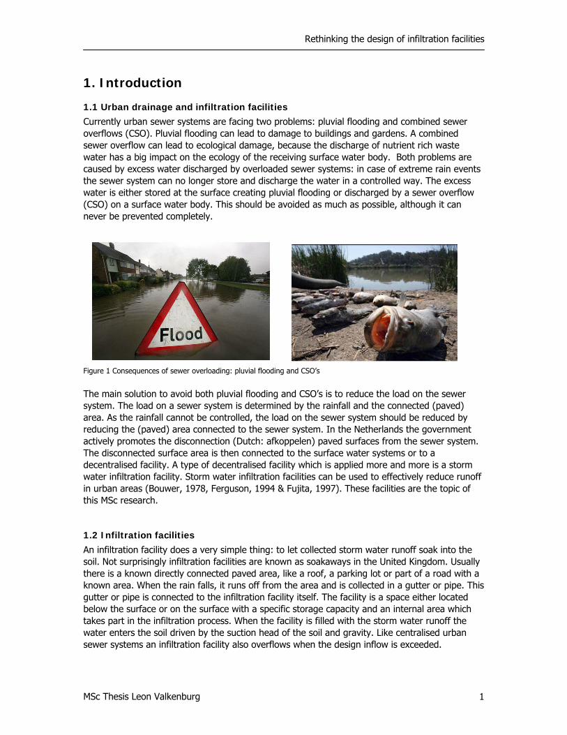
1.1 Urban drainage and infiltration facilities Currently urban sewer systems are facing two problems: pluvial flooding and combined sewer overflows (CSO). Pluvial flooding can lead to damage to buildings and gardens. A combined sewer overflow can lead to ecological damage, because the discharge of nutrient rich waste water has a big impact on the ecology of the receiving surface water body. Both problems are caused by excess water discharged by overloaded sewer systems: in case of extreme rain events the sewer system can no longer store and discharge the water in a controlled way. The excess water is either stored at the surface creating pluvial flooding or discharged by a sewer overflow (CSO) on a surface water body. This should be avoided as much as possible, although it can never be prevented completely.
Figure 1 Consequences of sewer overloading: pluvial flooding and CSO’s
The main solution to avoid both pluvial flooding and CSO’s is to reduce the load on the sewer system. The load on a sewer system is determined by the rainfall and the connected (paved) area. As the rainfall cannot be controlled, the load on the sewer system should be reduced by reducing the (paved) area connected to the sewer system. In the Netherlands the government actively promotes the disconnection (Dutch: afkoppelen) paved surfaces from the sewer system. The disconnected surface area is then connected to the surface water systems or to a decentralised facility. A type of decentralised facility which is applied more and more is a storm water infiltration facility. Storm water infiltration facilities can be used to effectively reduce runoff in urban areas (Bouwer, 1978, Ferguson, 1994 & Fujita, 1997). These facilities are the topic of this MSc research.
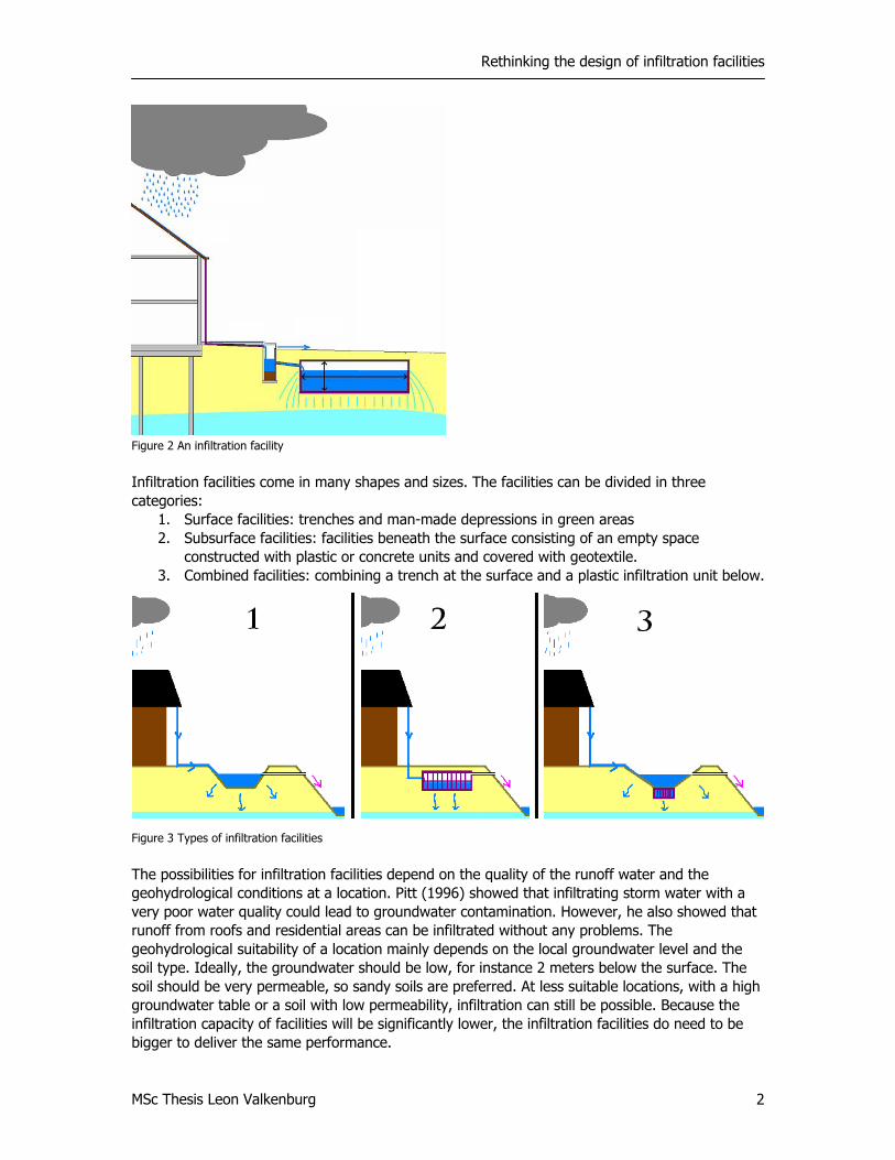
1.2 Infiltration facilities An infiltration facility does a very simple thing: to let collected storm water runoff soak into the soil. Not surprisingly infiltration facilities are known as soakaways in the United Kingdom. Usually there is a known directly connected paved area, like a roof, a parking lot or part of a road with a known area. When the rain falls, it runs off from the area and is collected in a gutter or pipe. This gutter or pipe is connected to the infiltration facility itself. The facility is a space either located below the surface or on the surface with a specific storage capacity and an internal area which takes part in the infiltration process. When the facility is filled with the storm water runoff the water enters the soil driven by the suction head of the soil and gravity. Like centralised urban sewer systems an infiltration facility also overflows when the design inflow is exceeded.
Rethinking the design of infiltration facilities
MSc Thesis Leon Valkenburg 2
Figure 2 An infiltration facility
Infiltration facilities come in many shapes and sizes. The facilities can be divided in three categories:
1. Surface facilities: trenches and man-made depressions in green areas 2. Subsurface facilities: facilities beneath the surface consisting of an empty space
constructed with plastic or concrete units and covered with geotextile. 3. Combined facilities: combining a trench at the surface and a plastic infiltration unit below.
Figure 3 Types of infiltration facilities
The possibilities for infiltration facilities depend on the quality of the runoff water and the geohydrological conditions at a location. Pitt (1996) showed that infiltrating storm water with a very poor water quality could lead to groundwater contamination. However, he also showed that runoff from roofs and residential areas can be infiltrated without any problems. The geohydrological suitability of a location mainly depends on the local groundwater level and the soil type. Ideally, the groundwater should be low, for instance 2 meters below the surface. The soil should be very permeable, so sandy soils are preferred. At less suitable locations, with a high groundwater table or a soil with low permeability, infiltration can still be possible. Because the infiltration capacity of facilities will be significantly lower, the infiltration facilities do need to be bigger to deliver the same performance.

Rethinking the design of infiltration facilities
MSc Thesis Leon Valkenburg 3
1.3 Scope of this research The scope of this research was rethinking the hydraulic design of infiltration facilities. Design methods for storm water infiltration facilities in the Netherlands and abroad have been in use for years now. They have been commonly accepted and are rarely questioned. However the assumptions, rules of thumb and guidelines used in these methods have a scientific basis which is unclear. The first step of this research is to question these current guidelines and point out the (scientific) uncertainties in them. The second step is to test and fill in the uncertainties by modelling facilities in an unsaturated zone model and measuring them in practice. The final step is to come up with an improved design method containing fewer uncertainties.
1.4 Research question How can the design of infiltration facilities be improved using modelling in an unsaturated zone model and measuring in facilities in practice?
1.5 Research method Answering the research question was done in four steps:
1. The scientific background of the processes which influence the hydraulic design (and performance) of infiltration facilities was summarised. This way the processes relevant for the performance and design of infiltration facilities could be identified.
2. The current design methods used in four countries were analysed. In this analysis the design guidelines were compared with each other and tested on scientific validity.
3. The influence of the design assumptions and uncertainties on the calculation of infiltration capacity was studied. This was done by modelling infiltration facilities in a unsaturated zone model and by measuring in infiltration facilities in the municipality of Ede.
4. Based on the measurements and the model results, the design method for infiltration facilities was refined.
1.6 Readers guide This report starts with explaining the scientific background of infiltration facilities in chapter 2. Chapter 3 contains the analysis of the current design methods. In chapter 4 the uncertainties in the infiltration capacity are studied and explained. Chapter 5 presents a refined design method based on the results from chapter 4. In the chapter 6 the conclusions and recommendations of the research are presented.
Rethinking the design of infiltration facilities
MSc Thesis Leon Valkenburg 4
2. Processes influencing infiltration facilities How does storm water infiltration actually work? As this research is focussed on the hydraulic design of storm water infiltration facilities, this chapter will take a closer look at the (hydrologic) processes influencing their hydraulic performance. Evidently these processes are also of big influence on the design of a facility. Basically the hydraulic performance of an infiltration facility is influenced by three processes. Like any facility that is involved in storing and discharging water, the facilities are governed by an inflow, an outflow and a reduction of capacity in time. Applying these aspects to infiltration facilities result in: 1. The urban runoff (the inflow): the amount of water expected to enter the facility. 2. The infiltration rate: the flux of water which infiltrates from the facility to the soil and the
groundwater. 3. The clogging: reduction of the infiltration rate due to chemical, biological and physical
clogging of the facility and the surrounding soil. All three of these processes will be explained in detail in this chapter.
2.1 Urban runoff Urban runoff in itself is influenced by two processes: rainfall and runoff generation. The question is how much water of a rain event will reach the inlet of an infiltration system. This section will describe the processes which are important for urban runoff generation. It will also introduce the main scientific method used in this research for calculating the amount of urban runoff.
2.1.1 Rainfall For the design of an urban drainage system the relevant characteristics of rainfall should be taken into account. Butler (2004) identified four aspects, expressed in question, which are included in rainfall analysis:
• Depth: how much rainfall (in mm) is generated by one storm? • Intensity: how much rainfall is generated per unit of time (in mm per hour)? • Duration: how much time (in minutes or hours) has elapsed between from the first drop
that has been caught till the last drop? • Frequency: how often does a specific rainfall event occur (in years)?
For a study which needs continuous rainfall data, the following aspect is also relevant: • Temporal variability: how is the rainfall divided over a specific time period (usually in
years)? To give answers to these questions long term observations of point rainfall have to be statistically represented. Like in all scientific disciplines various methods have been developed to do this. Below three main methods (Butler, 2004) for describing point rainfall will be discussed:
1. Depth-duration-frequency curve: Graphical representation of analysis of long term rainfall statistics; given a return period the rainfall depth is plotted against time.
2. Synthetic design storm: a synthetically generated rainfall event, with specific characteristics (variable intensity) to test drainage systems to their limits.
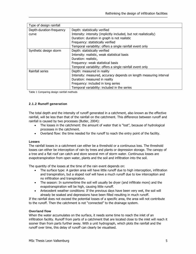
3. Rainfall series: historical rainfall records with a specific measuring interval. In table 1 three methods are compared on the 5 aspects mentioned before.
Rethinking the design of infiltration facilities
MSc Thesis Leon Valkenburg 5
Type of design rainfall Depth-duration-frequency curve
Depth: statistically verified Intensity: intensity (implicitly included, but not realistically) Duration: duration in graph is not realistic Frequency: statistically verified Temporal variability: offers a single rainfall event only
Synthetic design storm Depth: statistically verified Intensity: realistic, weak statistical basis Duration: realistic, Frequency: weak statistical basis Temporal variability: offers a single rainfall event only
Rainfall series Depth: measured in reality Intensity: measured, accuracy depends on length measuring interval Duration: measured in reality Frequency: included in long series Temporal variability: included in the series
Table 1 Comparing design rainfall methods
2.1.2 Runoff generation The total depth and the intensity of runoff generated in a catchment, also known as the effective rainfall, will be less than that of the rainfall on the catchment. This difference between runoff and rainfall is caused by two processes (Butler, 2004):
• The losses in the catchment: the amount of water that is “lost”, because of hydrological processes in the catchment.
• Overland flow: the time needed for the runoff to reach the entry point of the facility. Losses The rainfall losses in a catchment can either be a threshold or a continuous loss. The threshold losses can either be interception of rain by trees and plants or depression storage. The canopy of a tree and a flat roof can catch and store several mm of storm water. Continuous losses are evapotranspiration from open water, plants and the soil and infiltration into the soil. The quantity of the losses at the time of the rain event depends on:
• The surface type: A garden area will have little runoff due to high interception, infiltration and transpiration, but a sloped roof will have a much runoff due to low interception and no infiltration and transpiration.
• The season: In summertime the soil will usually be dryer (and infiltrate more) and the evapotranspiration will be high, causing little runoff.
• Antecedent weather conditions: If the previous days have been very wet, the soil will already be soaked and depressions have been filled resulting in much runoff.
If the rainfall does not exceed the potential losses of a specific area, the area will not contribute to the runoff. Then the catchment is not “connected” to the drainage system. Overland flow When the water accumulates on the surface, it needs some time to reach the inlet of an infiltration facility. Runoff from parts of a catchment that are located close to the inlet will reach it sooner than from parts further away. With a unit hydrograph, which plots the rainfall and the runoff over time, this delay of runoff can clearly be visualised.
Rethinking the design of infiltration facilities
MSc Thesis Leon Valkenburg 6
The rational method (first developed by Mulvaney in 1850) is a scientific to quantify both the effects of losses and overland flow in the catchment on the runoff generation. It is commonly used for the design of storm water sewer systems can be used. It reads as follows: Qr = CAitc (2.1) Where: Qr = runoff [L3T-1] C = runoff coefficient [-] A = connected area [L2] itc = rainfall intensity depending on the time of concentration[LT-1] The runoff is calculated with a runoff coefficient, the connected area and the rainfall intensity. The runoff coefficient depends on the surface type and implicitly takes into account the losses. The connected area is assumed to be a known constant. The rainfall intensity depends on the time of concentration (tc) of the catchment. This is the time needed for surface runoff to reach the inlet of the facility from the remotest part of the catchment, taking into account overland flow. The tc is combines the time of entry in the facility te and the time of flow inside the system tf: tc = te+tf (2.2) The rational method has got some clear limitations, which are mainly caused by assuming the runoff coefficient to be constant. The “real” coefficient is never constant in reality. In reality it is affected by all processes mentioned in the beginning of this section. These processes are not constant. For instance a roof can already be wet or depressions can be filled by rain on the day before. Considering this the runoff coefficients are applied conservatively.
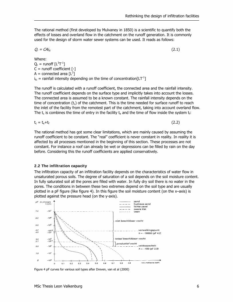
2.2 The infiltration capacity The infiltration capacity of an infiltration facility depends on the characteristics of water flow in unsaturated porous soils. The degree of saturation of a soil depends on the soil moisture content. In fully saturated soil all the pores are filled with water. In fully dry soil there is no water in the pores. The conditions in between these two extremes depend on the soil type and are usually plotted in a pF figure (like figure 4). In this figure the soil moisture content (on the x–axis) is plotted against the pressure head (on the y-axis).
Figure 4 pF curves for various soil types after Dreven, van et al (2000)
Rethinking the design of infiltration facilities
MSc Thesis Leon Valkenburg 7
q K H= − ∇
For the design of infiltration facilities the information in figure 4 should be translated to groundwater fluxes. There are however many steps in between. Water flow in unsaturated conditions is a very complex process (Tindal et al., 1999) and this naturally leads to complex calculations. So how can unsaturated flow accurately be described?
2.2.1 Darcy’s description of groundwater flow The basics of groundwater flow are commonly described by Darcy’s law. This law is applicable for saturated homogenous porous media and laminar flow in the pores, which is governed by the gravity or the hydraulic gradient only: (2.3) Where:
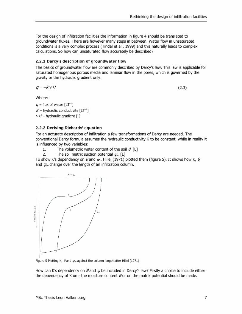
2.2.2 Deriving Richards’ equation For an accurate description of infiltration a few transformations of Darcy are needed. The conventional Darcy formula assumes the hydraulic conductivity K to be constant, while in reality it is influenced by two variables:
1. The volumetric water content of the soil θ [L] 2. The soil matrix suction potential ψm [L]
To show K’s dependency on θ and ψm Hillel (1971) plotted them (figure 5). It shows how K, θ and ψm change over the length of an infiltration column.
Figure 5 Plotting K, θ and ψm against the column length after Hillel (1971)
How can K’s dependency on θ and ψ be included in Darcy’s law? Firstly a choice to include either the dependency of K on r the moisture content θ or on the matrix potential should be made.
-1
-1
flux of water [LT ]
hydraulic conductivity [LT ]hydraulic gradient [-]
qK
H
=
=∇ =
Rethinking the design of infiltration facilities
MSc Thesis Leon Valkenburg 8
( ) ( )q K Kz
ψ θθ θθ
∂ ∂⎛ ⎞= − − −⎜ ⎟∂ ∂⎝ ⎠
( )q K Hθ= − ∇
( ) ( )q K h zθ= − ∇ +
( )(1 )mq Kzψ
θ∂
= − −∂
m mdz d zψ ψ θ
θ∂ ∂
=∂ ∂
1 mq Kzψ∂⎛ ⎞= − −⎜ ⎟∂⎝ ⎠
Tindall et al.(1999) use K dependent on θ, because potential hysteresis due to ψm is then avoided. This step yields: (2.4) Adding ψm in the form of h to the hydraulic gradient H= h+z leads to: (2.5) One dimensional form to flow in the z direction and substituting -ψm for h gives: (2.6) Assuming ψ is a single valued function of θ: (2.7) Combing (6) and (7) finally yields the equation developed by Richards in 1931: (2.8) Many scientists (Gardner, Mualem & Van Genuchten) have produced methods for calculating K and other variables within Richards’ equation.
2.2.3 Applying Richards’ equation How can Richards’ equation be used in water resources management practice? Water resources management is about quantifying water flow, so how can Richards’ equation in the research be used to quantify infiltration? The challenge is that Richards’ equation is a non linear differential equation. In other words, it is too complex to calculate directly. The several additions from scientists like Mualem and Van Genuchten have improved the description of infiltration and reduced complexity in the calculations. However to include all the old and new theories in the calculation is a big challenge. Fortunately computers have made complex calculations a lot easier. Computer models facilitate the simulation of infiltration without the need of elaborate programming. A good example of an accessible model is HYDRUS, which includes Richards’ equation and all relevant additions and, above all, is scientifically verified (Simunek et al, 2008).
2.2.4 Simplifications of Richards’ equation Horton For a direct calculation of the infiltration rate without the help of computers Richards’ equation needs to be simplified. One way is to assume the K not dependent on θ, this results in: (2.9) This formula is actually a form of Horton’s equation of infiltration developed in 1933. Horton determined empirically how the infiltration rate decreased from an initial infiltration rate to an end infiltration rate at the surface. In fact he was describing the influence of the matrix potential on the infiltration rate.
Rethinking the design of infiltration facilities
MSc Thesis Leon Valkenburg 9
0( ) ( )( )
( )mH t L t
q t KL t
ψ+ +⎛ ⎞= − ⎜ ⎟
⎝ ⎠
gK k ρη
=
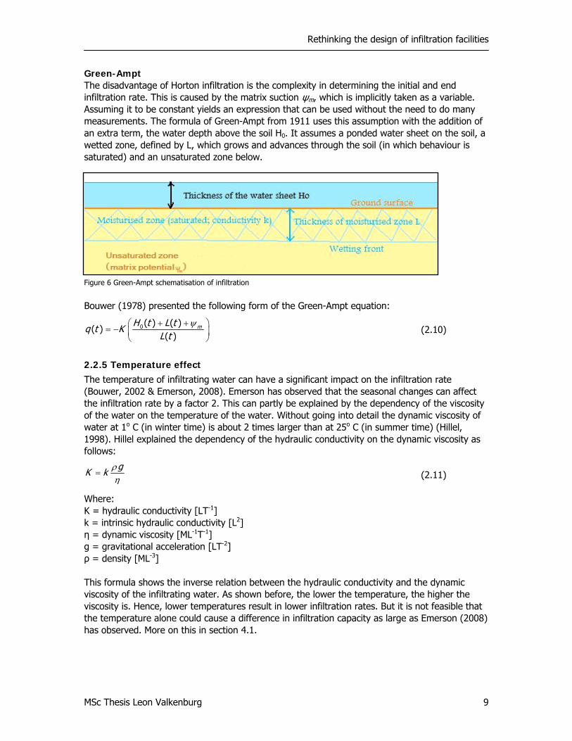
Green-Ampt The disadvantage of Horton infiltration is the complexity in determining the initial and end infiltration rate. This is caused by the matrix suction ψm, which is implicitly taken as a variable. Assuming it to be constant yields an expression that can be used without the need to do many measurements. The formula of Green-Ampt from 1911 uses this assumption with the addition of an extra term, the water depth above the soil H0. It assumes a ponded water sheet on the soil, a wetted zone, defined by L, which grows and advances through the soil (in which behaviour is saturated) and an unsaturated zone below.
Figure 6 Green-Ampt schematisation of infiltration
Bouwer (1978) presented the following form of the Green-Ampt equation: (2.10)
2.2.5 Temperature effect The temperature of infiltrating water can have a significant impact on the infiltration rate (Bouwer, 2002 & Emerson, 2008). Emerson has observed that the seasonal changes can affect the infiltration rate by a factor 2. This can partly be explained by the dependency of the viscosity of the water on the temperature of the water. Without going into detail the dynamic viscosity of water at 1o C (in winter time) is about 2 times larger than at 25o C (in summer time) (Hillel, 1998). Hillel explained the dependency of the hydraulic conductivity on the dynamic viscosity as follows: (2.11) Where: K = hydraulic conductivity [LT-1] k = intrinsic hydraulic conductivity [L2] η = dynamic viscosity [ML-1T-1] g = gravitational acceleration [LT-2] ρ = density [ML-3] This formula shows the inverse relation between the hydraulic conductivity and the dynamic viscosity of the infiltrating water. As shown before, the lower the temperature, the higher the viscosity is. Hence, lower temperatures result in lower infiltration rates. But it is not feasible that the temperature alone could cause a difference in infiltration capacity as large as Emerson (2008) has observed. More on this in section 4.1.
Rethinking the design of infiltration facilities
MSc Thesis Leon Valkenburg 10
0( ) 2( ) m
cc
H tq t K
Lψ−
=
2.3 Clogging In all processes in which water enters a soil mass clogging will occur. Pollution particles dissolved and suspended in water will slowly fill the pores of the soil mass. The soil will in this case always act as a filter. Naturally this process is often used on purpose: in drinking water treatment the raw water is lead trough a sand filter in which the pollutants are contained. However storm water infiltration facilities are vulnerable to clogging, because clogging leads to a reduction of the infiltration capacity(Bouwer, 1978, Rinck-Pfeiffer, 2000, Dechesne, 2004 & Siwardene, 2007), which eventually could lead to failure of the facility. This section will describe the clogging process and methods to quantify its reduction of the hydraulic capacity of infiltration facilities. 2.3.1 The clogging process Clogging can be described as the reduction of the infiltration rate by reduction of the hydraulic conductivity and the porosity of the soil. Bouwer (2002) identifies three different causes of clogging:
• Physical clogging due to an accumulation of inorganic and organic suspended solids. • Biological clogging due to an accumulation of algae and bacterial flocks on the infiltrating
surface. • Chemical clogging due to “precipitation” of different chemicals in the soil, such as
phosphate and calcium carbonate. Of these three processes infiltration facilities are affected most by physical clogging (Rinck-Pfeiffer, 2000 & Siwardene, 2007). This physical clogging is caused by sediments suspended and dissolved in the storm water runoff. These particles will form a clogging layer at the filter/soil interface. Siwardene (2007) found that clogging is driven by sediment particles less than 6 μm, because there are more likely to reach the filter/soil interface. Also, facilities with a fluctuating water level were found to be more prone to clogging than facilities with a stable water level. 2.3.2 Quantifying clogging Quantifying the reduction of the infiltration rate by clogging is complex, because it is very case dependent. The time elapsed until a facility is clogged, depends on many factors. The type of connected paved area; the type of facility; the presence of pre-treatment; the maintenance regime or the design of the facility itself; it all can play a role. Because of this the quantification of clogging has been limited to theoretical and laboratory studies. Deshesne (2004) and Bouwer (2002) have tried to develop similar ways to determine the infiltration rate for a clogged basin. The expression is similar to Bouwer’s presentation of Green-Ampt (2.10): (2.12) Where q(t) = infiltration rate [LT-1] Kc = hydraulic conductivity of the clogging layer [LT-1] H0 = water level in facility [L] Lc = Thickness of clogging layer [L] Ψm = matrix suction potential [L] The infiltration rate in this formula depends on the hydraulic conductivity of the clogging layer water level in the facility, the matrix suction potential divided by the thickness of the clogging layer.
Rethinking the design of infiltration facilities
MSc Thesis Leon Valkenburg 11
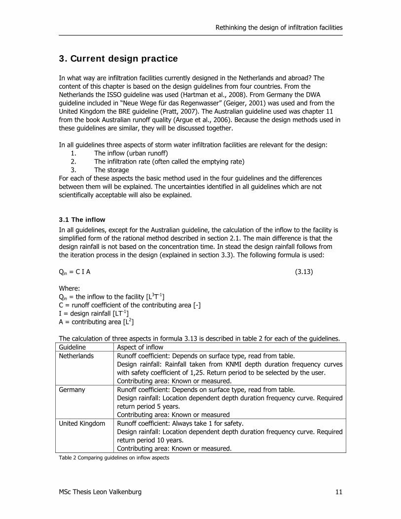
3. Current design practice In what way are infiltration facilities currently designed in the Netherlands and abroad? The content of this chapter is based on the design guidelines from four countries. From the Netherlands the ISSO guideline was used (Hartman et al., 2008). From Germany the DWA guideline included in “Neue Wege für das Regenwasser” (Geiger, 2001) was used and from the United Kingdom the BRE guideline (Pratt, 2007). The Australian guideline used was chapter 11 from the book Australian runoff quality (Argue et al., 2006). Because the design methods used in these guidelines are similar, they will be discussed together. In all guidelines three aspects of storm water infiltration facilities are relevant for the design:
1. The inflow (urban runoff) 2. The infiltration rate (often called the emptying rate) 3. The storage
For each of these aspects the basic method used in the four guidelines and the differences between them will be explained. The uncertainties identified in all guidelines which are not scientifically acceptable will also be explained.
3.1 The inflow In all guidelines, except for the Australian guideline, the calculation of the inflow to the facility is simplified form of the rational method described in section 2.1. The main difference is that the design rainfall is not based on the concentration time. In stead the design rainfall follows from the iteration process in the design (explained in section 3.3). The following formula is used: Qin = C I A (3.13) Where: Qin = the inflow to the facility [L3T-1] C = runoff coefficient of the contributing area [-] I = design rainfall [LT-1] A = contributing area [L2] The calculation of three aspects in formula 3.13 is described in table 2 for each of the guidelines. Guideline Aspect of inflow Netherlands Runoff coefficient: Depends on surface type, read from table.
Design rainfall: Rainfall taken from KNMI depth duration frequency curves with safety coefficient of 1,25. Return period to be selected by the user. Contributing area: Known or measured.
Germany Runoff coefficient: Depends on surface type, read from table. Design rainfall: Location dependent depth duration frequency curve. Required return period 5 years. Contributing area: Known or measured
United Kingdom Runoff coefficient: Always take 1 for safety. Design rainfall: Location dependent depth duration frequency curve. Required return period 10 years. Contributing area: Known or measured.
Table 2 Comparing guidelines on inflow aspects
Rethinking the design of infiltration facilities
MSc Thesis Leon Valkenburg 12
In Australia no design storm is used. In stead the facility is designed on hydrologic effectiveness, the fraction of the cumulative annual precipitation that should be captured by the facility(varying from 40%-95%). This method does include the use of area specific runoff coefficients. The following uncertainties in the calculation of the inflow can be identified given the theory described in section 2.1:
• DDF-curves are not very suitable for use as design rainfall (explained in section 2.1.1). • A constant runoff coefficient does not include the variability of runoff in reality. • As the rainfall intensity is not based on the concentration time, no delay in runoff is
included. • Extreme rainfall (rainfall which exceeds the design rainfall) is not considered.
Although these uncertainties can be significant, they will not be looked into more detail for this research. Much other research has already been done on this.
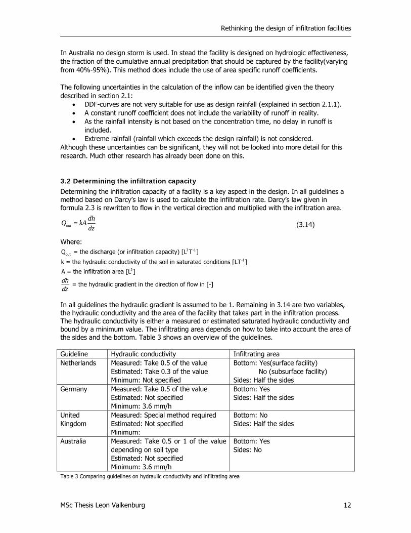
3.2 Determining the infiltration capacity Determining the infiltration capacity of a facility is a key aspect in the design. In all guidelines a method based on Darcy’s law is used to calculate the infiltration rate. Darcy’s law given in formula 2.3 is rewritten to flow in the vertical direction and multiplied with the infiltration area.
(3.14)
Where:
In all guidelines the hydraulic gradient is assumed to be 1. Remaining in 3.14 are two variables, the hydraulic conductivity and the area of the facility that takes part in the infiltration process. The hydraulic conductivity is either a measured or estimated saturated hydraulic conductivity and bound by a minimum value. The infiltrating area depends on how to take into account the area of the sides and the bottom. Table 3 shows an overview of the guidelines. Guideline Hydraulic conductivity Infiltrating area Netherlands Measured: Take 0.5 of the value
Estimated: Take 0.3 of the value Minimum: Not specified
Bottom: Yes(surface facility) No (subsurface facility) Sides: Half the sides
Germany Measured: Take 0.5 of the value Estimated: Not specified Minimum: 3.6 mm/h
Bottom: Yes Sides: Half the sides
United Kingdom
Measured: Special method required Estimated: Not specified Minimum:
Bottom: No Sides: Half the sides
Australia Measured: Take 0.5 or 1 of the value depending on soil type Estimated: Not specified Minimum: 3.6 mm/h
Bottom: Yes Sides: No
Table 3 Comparing guidelines on hydraulic conductivity and infiltrating area
=outdhQ kAdz
3 -1out
-1
2
Q = the discharge (or infiltration capacity) [L T ]
k = the hydraulic conductivity of the soil in saturated conditions [LT ]
A = the infiltration area [L ]
= the hydraulic gradient in the diredhdz
ction of flow in [-]

Rethinking the design of infiltration facilities
MSc Thesis Leon Valkenburg 13
Many uncertainties in the calculation of the infiltration rate can be identified given the theory described in section 2.2 and 2.3. On the field of the design formula and related assumptions these uncertainties can be identified:
• Darcy’s law for saturated flow cannot be applied to unsaturated flow. • The hydraulic gradient in Darcy’s law cannot be assumed to be 1; it is significantly higher
in infiltration. • The saturated hydraulic conductivity (used in the design) either measured or estimated
contains many uncertainties in itself: the heterogeneity of the soil is not included, the unsaturated conductivity always less than saturated conductivity, the conductivity is not constant and depends on the amount of entrapped air, soil moisture content and suction head of the soil matrix and conductivity can be affected by temperature.
• Infiltration through the sides of a facility is not one dimensional and cannot be described one dimensionally like infiltration through the bottom.
• Taking into account half of the sides assumes a constant water level during the infiltration process. In reality the water level is variable. The assumption underestimates the area of the sides that takes part in infiltration for the infiltration of the first half of the storage in the facility and overestimates it for the second half.
On the field of design aspects:
• Few recommendations are made about the optimal shape of an infiltration facility. It is unclear what the optimal ratio is between bottom area and side area of a facility to maximise infiltration.
On the field of (geo)hydrologic boundary conditions:
• The influence of the groundwater on the infiltration rate is unclear, so it is not known whether the design formulas still hold in cases with a low or high groundwater level.
• Although some guidelines give recommendations about the soil type (and hydraulic conductivity) required for infiltration, the basis of these recommendations is unclear.
On the field of clogging:
• In the calculation the hydraulic conductivity of the soil at the project location is taken as the normative value for the conductivity. Due to clogging the conductivity of either the soil or the geotextile at the soil-water interface could be limiting the infiltration rate and not the soil at the project location.
• Complete clogging of the bottom till the point it no longer takes part in infiltration has not been observed in practice.
3.3 Determining the dimensions and the storage If the inflow and the infiltration rate have been determined the storage can be calculated. Sometimes the required storage can be bounded by local regulations; the guidelines do not have requirements on this point. Formula 3.15 is used to determine the storage needed in a facility:
0
( ) ( )t
in outMax S Q Q dt= −∫ (3.15)
Where: S = storage in [L3] Qin = total inflow for the given/chosen time interval [L3T-1] Qout = total outflow for the given/chosen time interval [L3T-1] t = duration of design rainfall [T]
Rethinking the design of infiltration facilities
MSc Thesis Leon Valkenburg 14
;empty
out avg
STQ
=
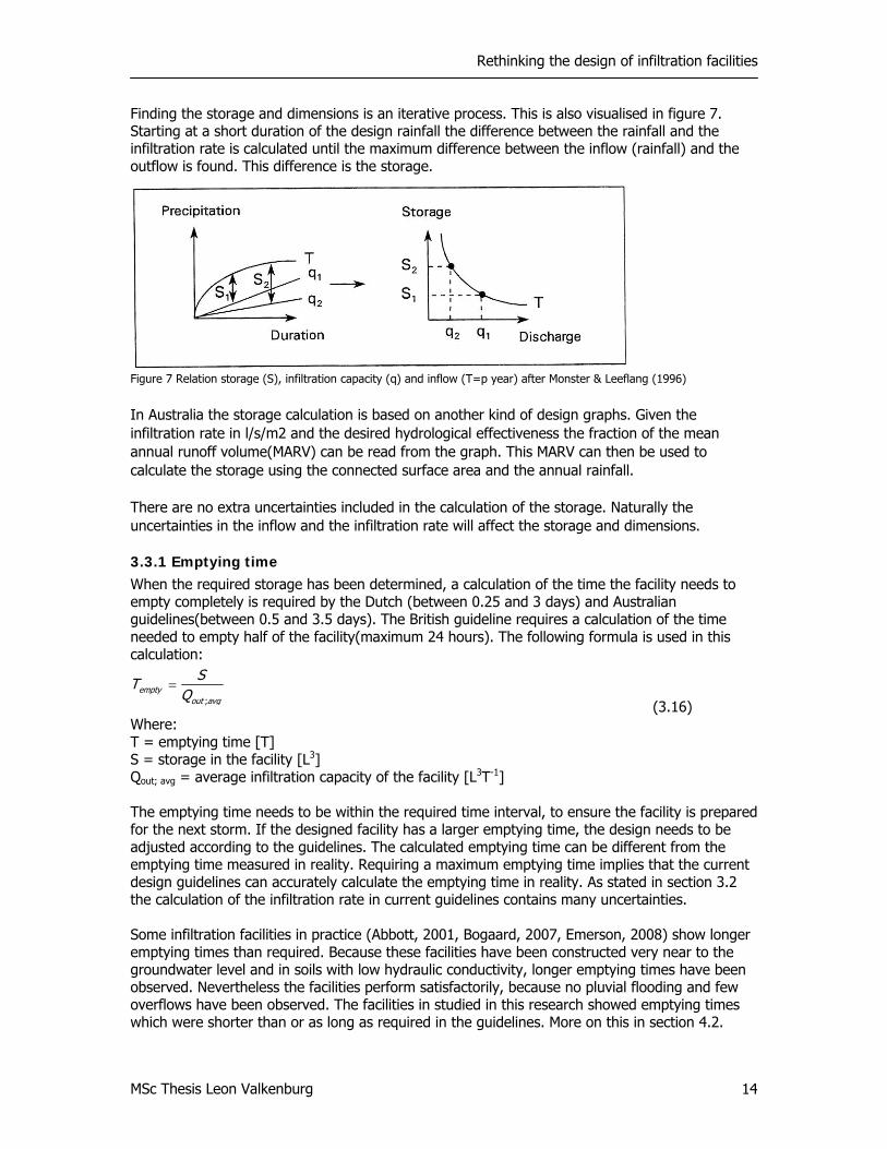
Finding the storage and dimensions is an iterative process. This is also visualised in figure 7. Starting at a short duration of the design rainfall the difference between the rainfall and the infiltration rate is calculated until the maximum difference between the inflow (rainfall) and the outflow is found. This difference is the storage.
Figure 7 Relation storage (S), infiltration capacity (q) and inflow (T=p year) after Monster & Leeflang (1996)
In Australia the storage calculation is based on another kind of design graphs. Given the infiltration rate in l/s/m2 and the desired hydrological effectiveness the fraction of the mean annual runoff volume(MARV) can be read from the graph. This MARV can then be used to calculate the storage using the connected surface area and the annual rainfall. There are no extra uncertainties included in the calculation of the storage. Naturally the uncertainties in the inflow and the infiltration rate will affect the storage and dimensions.
3.3.1 Emptying time When the required storage has been determined, a calculation of the time the facility needs to empty completely is required by the Dutch (between 0.25 and 3 days) and Australian guidelines(between 0.5 and 3.5 days). The British guideline requires a calculation of the time needed to empty half of the facility(maximum 24 hours). The following formula is used in this calculation: (3.16) Where: T = emptying time [T] S = storage in the facility [L3] Qout; avg = average infiltration capacity of the facility [L3T-1] The emptying time needs to be within the required time interval, to ensure the facility is prepared for the next storm. If the designed facility has a larger emptying time, the design needs to be adjusted according to the guidelines. The calculated emptying time can be different from the emptying time measured in reality. Requiring a maximum emptying time implies that the current design guidelines can accurately calculate the emptying time in reality. As stated in section 3.2 the calculation of the infiltration rate in current guidelines contains many uncertainties. Some infiltration facilities in practice (Abbott, 2001, Bogaard, 2007, Emerson, 2008) show longer emptying times than required. Because these facilities have been constructed very near to the groundwater level and in soils with low hydraulic conductivity, longer emptying times have been observed. Nevertheless the facilities perform satisfactorily, because no pluvial flooding and few overflows have been observed. The facilities in studied in this research showed emptying times which were shorter than or as long as required in the guidelines. More on this in section 4.2.
Rethinking the design of infiltration facilities
MSc Thesis Leon Valkenburg 15
4. Studying the infiltration capacity Which uncertainties affect the performance of infiltration facilities in practice the most? In what way can the infiltration capacity be calculated accurately and in what way can the design be optimised to maximise the infiltration capacity? The goal of this chapter was to improve the assumptions and reduce the uncertainties in the infiltration rate as much as possible. This was done by modelling in Hydrus 2D or by measuring infiltration facilities in practice.
4.1 Modelling infiltration facilities A computer model can assist in studying infiltration in more detail. In this section an unsaturated zone model was used to study several of the uncertainties identified in chapter 3. To study these uncertainties this model should be able to:
• Quantify infiltration in the unsaturated zone in time. • Include Richards equation explained in section 2.2 to ensure reliable calculation of the
infiltration process. • Include multidimensional flow, in horizontal and vertical direction. • Able to model different types of infiltration facilities. • Able to model different (geo)hydrological conditions, such as groundwater level and soil
types.
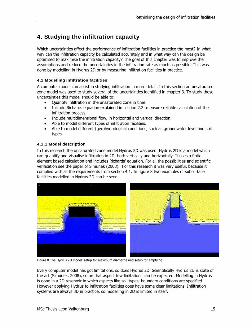
4.1.1 Model description In this research the unsaturated zone model Hydrus 2D was used. Hydrus 2D is a model which can quantify and visualise infiltration in 2D, both vertically and horizontally. It uses a finite element based calculation and includes Richards’ equation. For all the possibilities and scientific verification see the paper of Simunek (2008). For this research it was very useful, because it complied with all the requirements from section 4.1. In figure 8 two examples of subsurface facilities modelled in Hydrus 2D can be seen.
Figure 8 The Hydrus 2D model: setup for maximum discharge and setup for emptying
Every computer model has got limitations, so does Hydrus 2D. Scientifically Hydrus 2D is state of the art (Simunek, 2008), so on that aspect few limitations can be expected. Modelling in Hydrus is done in a 2D reservoir in which aspects like soil types, boundary conditions are specified. However applying Hydrus to infiltration facilities does have some clear limitations. Infiltration systems are always 3D in practice, so modelling in 2D is limited in itself.
Rethinking the design of infiltration facilities
MSc Thesis Leon Valkenburg 16
Also, aspects which are important for infiltration, clogging, the type of facility (concrete or plastic unit with geotextile) and the heterogeneity of the soil, cannot be modelled easily. This is primarily because they are very case dependent and there are no data available which are useful for modelling these aspects. Because these aspects can prolong the emptying time of a facility and cannot be included in Hydrus, the value of studying the emptying time of facilities with Hydrus is limited. Real-life measurements of emptying times are essential here.
4.1.2 Setup of model Hydrus was used to study the uncertainties in the calculation of the infiltration rate identified in section 3.2. The limitations described in section 4.1.1 had to be considered as well. The focus for modelling was to find out the accuracy of the Darcy-based calculation used in the guidelines in describing infiltration. The calculation of the guidelines is done with two design models:
• Darcy constant: assuming a constant outflow from a facility with the water level constant at half the height of the sides. The bottom area is not included in the infiltrating area.
• Darcy dynamic: dynamic outflow dependent on the water level in the facility. The bottom area is not included in the infiltrating area.
Hydrus was used to model an infiltration facility and compare the Hydrus’ results to the results calculated with the design models. The following parameters were constant throughout the modelling, unless it was the parameter on which the comparison was made:
• The facility: subsurface facility of 2 m x 0.5 m (width x height). • The groundwater level: 1.5 m below bottom level of facility • The soil type: loamy sand (saturated hydraulic conductivity ks = 1 m/d, residual
moisture content θr = 0.065, saturated moisture content θs = 0.41 ) • Initial moisture content θi: 0.08 • Temperature of water and soil: 20 0C • Bottom was assumed not to be clogged (different than in the design models)
The comparison was done on two aspects (both model setups can be seen in figure 8):
• The maximum infiltration capacity: the discharge after 0.5 hour given a constant maximum water level in the facility is simulated. The maximum infiltration capacity is important because it can affect the calculated storage significantly (see figure 7).
• The emptying time, the time needed for a facility to empty.
The design formula (primary) was compared on various parameters, which can affect the infiltration capacity of a facility and can vary significantly per location:
1. Influence groundwater level 2. Influence soil type (expressed in the hydraulic conductivity). 3. Influence initial moisture content 4. Influence shape of facility 5. Influence clogged bottom 6. Influence temperature of the water and soil
4.1.3 Results In this section the results of the Hydrus modelling are presented. In all graphs used for comparing the maximum discharge, the maximum discharge calculated with the Darcy constant design formula was made equal to 1. This eases comparison of the design formula with the modelled result of Hydrus. The emptying time is expressed in hours. Graphs plotting the infiltration process itself can be found in annex I.
Rethinking the design of infiltration facilities
MSc Thesis Leon Valkenburg 17
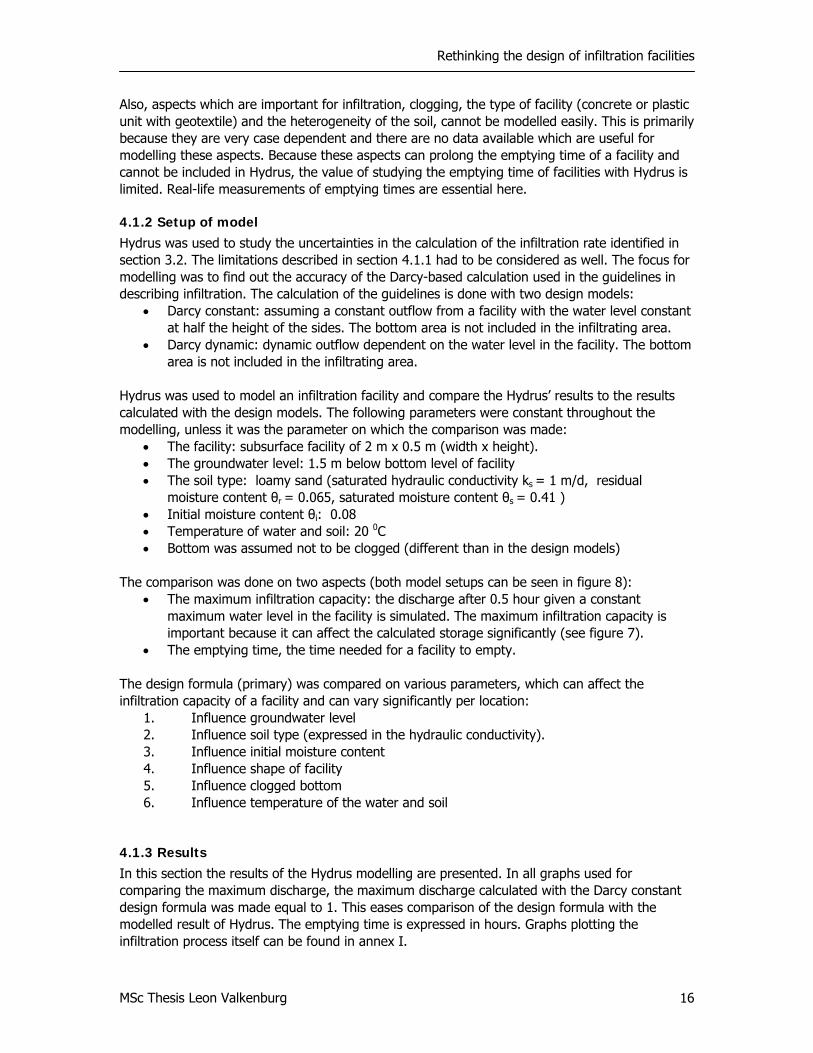
Influence groundwater level (groundwater level: 0.5 m above bottom level – 2 m below bottom level) Not surprisingly the groundwater level significantly affects both the emptying time and the infiltration rate of an infiltration facility. As figure 9 shows, the lower the groundwater level the higher the discharge of the infiltration facility of 2 m x 0.5 m (width x height). The discharge from a facility with a groundwater level 2 meters below its bottom was up to 3 times higher than from the same facility with a groundwater level directly below its bottom. The facility only emptied completely, when the groundwater level was more than 0.25 m below the bottom. The emptying time also decreased exponentially until the influence of the groundwater level was negligible. As stated in section 3.2 the design formula (Darcy constant and Darcy dynamic) did not take into account varying groundwater levels. This could lead to an underestimation of the discharge and overestimation of the emptying time. Hydrus showed a initial discharge to 30 times higher (15 for Darcy dynamic) from facilities with a low groundwater level up and an emptying time up to 10 times shorter (15 times for Darcy dynamic). In cases with a higher groundwater level the design formula predicted the discharge and the emptying time more accurately.
Figure 9 Influence groundwater level on discharge and emptying time
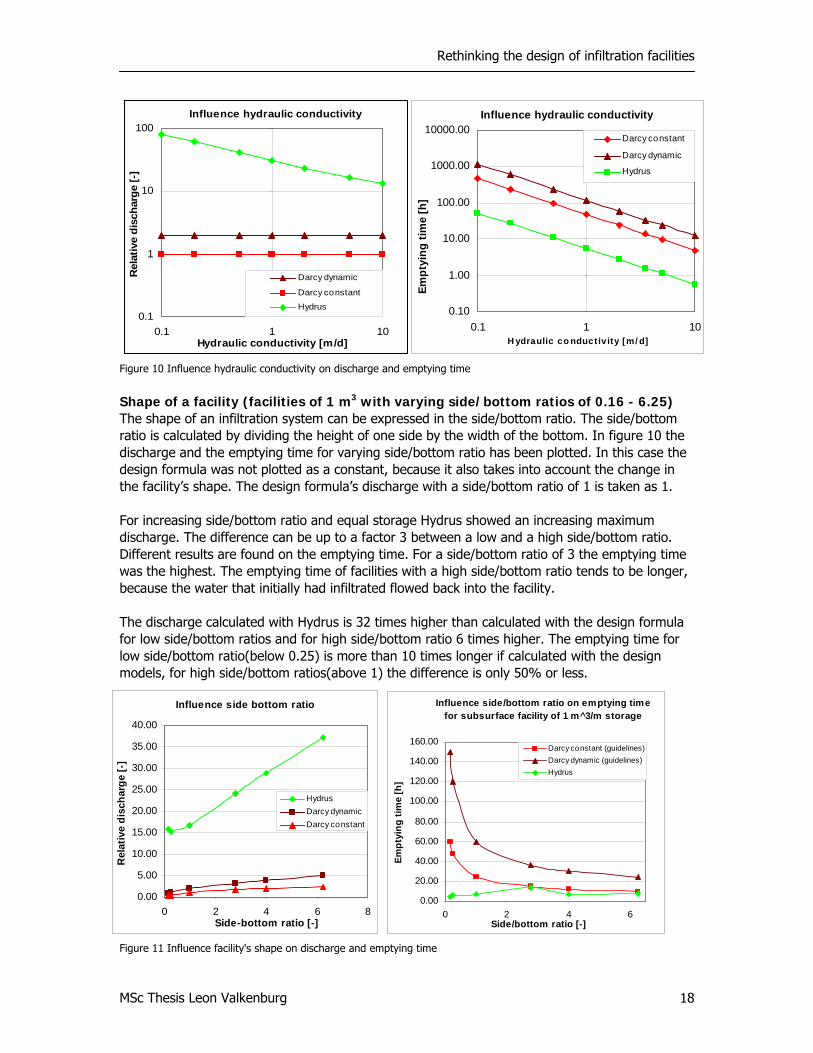
Influence hydraulic conductivity (hydraulic conductivity 0.1 m/d - 10 m/d) Evidently the hydraulic conductivity of the soil also has a big influence on the infiltration rate and the emptying time of a facility. In the design formula a linear increase in conductivity gave linear increase in the infiltration rate. However the Hydrus results in figure 10 (in log scale) showed a different pattern. The discharge calculated with the design formula was made 1 here. For low hydraulic conductivity (around 0.1 m/d) discharge was much higher and the emptying time much shorter than expected on basis of the design formula. The difference between the modelled discharge and emptying rate and the ones calculated with the Darcy constant and dynamic is also very big. For low conductivity Hydrus calculated a maximum discharge which is 80 times higher than calculated with the design formula, for high conductivity it was around 12 times higher. Hydrus also showed emptying times which were consistently 9 times shorter than the emptying times calculated with the design formula.
Influence groundwater level
0
5
10
15
20
25
30
35
-0.5 0 0.5 1 1.5 2Depth groundwater level below bottom [m]
Rel
ativ
e di
scha
rge
Darcy dynamic
Darcy constant
Hydrus
Hydrus no GWL
Influence groundwater level
0
10
20
30
40
50
60
70
80
0 0.5 1 1.5 2 2.5Gro undwater level belo w bo tto m [m]
Empt
yin
g ti
me
[h
]
Darcy constant Darcy dynamic Hydrus Hydrus no groundwater
Rethinking the design of infiltration facilities
MSc Thesis Leon Valkenburg 18
Figure 10 Influence hydraulic conductivity on discharge and emptying time
Shape of a facility (facilities of 1 m3 with varying side/bottom ratios of 0.16 - 6.25) The shape of an infiltration system can be expressed in the side/bottom ratio. The side/bottom ratio is calculated by dividing the height of one side by the width of the bottom. In figure 10 the discharge and the emptying time for varying side/bottom ratio has been plotted. In this case the design formula was not plotted as a constant, because it also takes into account the change in the facility’s shape. The design formula’s discharge with a side/bottom ratio of 1 is taken as 1. For increasing side/bottom ratio and equal storage Hydrus showed an increasing maximum discharge. The difference can be up to a factor 3 between a low and a high side/bottom ratio. Different results are found on the emptying time. For a side/bottom ratio of 3 the emptying time was the highest. The emptying time of facilities with a high side/bottom ratio tends to be longer, because the water that initially had infiltrated flowed back into the facility. The discharge calculated with Hydrus is 32 times higher than calculated with the design formula for low side/bottom ratios and for high side/bottom ratio 6 times higher. The emptying time for low side/bottom ratio(below 0.25) is more than 10 times longer if calculated with the design models, for high side/bottom ratios(above 1) the difference is only 50% or less.
Figure 11 Influence facility's shape on discharge and emptying time
Influence side/bottom ratio on emptying time for subsurface facility of 1 m^3/m storage
0.00
20.00
40.00
60.00
80.00
100.00
120.00
140.00
160.00
0 2 4 6Side/bottom ratio [-]
Empt
ying
tim
e [h
]
Darcy constant (guidelines)Darcy dynamic (guidelines)Hydrus
Influence hydraulic conductivity
0.1
1
10
100
0.1 1 10Hydraulic conductivity [m/d]
Rel
ativ
e di
scha
rge
[-]
Darcy dynamic
Darcy constant
Hydrus
Influence side bottom ratio
0.00
5.00
10.00
15.00
20.00
25.00
30.00
35.00
40.00
0 2 4 6 8Side-bottom ratio [-]
Rel
ativ
e di
scha
rge
[-]
HydrusDarcy dynamicDarcy constant
Influence hydraulic conductivity
0.10
1.00
10.00
100.00
1000.00
10000.00
0.1 1 10H ydraulic co nduct iv ity [m/ d]
Empt
ying
tim
e [h
]
Darcy constant
Darcy dynamic
Hydrus
Rethinking the design of infiltration facilities
MSc Thesis Leon Valkenburg 19
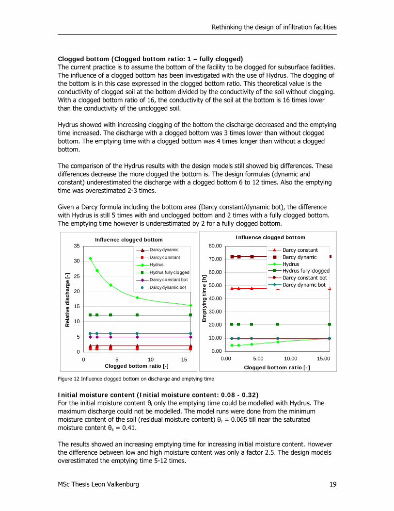
Clogged bottom (Clogged bottom ratio: 1 – fully clogged) The current practice is to assume the bottom of the facility to be clogged for subsurface facilities. The influence of a clogged bottom has been investigated with the use of Hydrus. The clogging of the bottom is in this case expressed in the clogged bottom ratio. This theoretical value is the conductivity of clogged soil at the bottom divided by the conductivity of the soil without clogging. With a clogged bottom ratio of 16, the conductivity of the soil at the bottom is 16 times lower than the conductivity of the unclogged soil. Hydrus showed with increasing clogging of the bottom the discharge decreased and the emptying time increased. The discharge with a clogged bottom was 3 times lower than without clogged bottom. The emptying time with a clogged bottom was 4 times longer than without a clogged bottom. The comparison of the Hydrus results with the design models still showed big differences. These differences decrease the more clogged the bottom is. The design formulas (dynamic and constant) underestimated the discharge with a clogged bottom 6 to 12 times. Also the emptying time was overestimated 2-3 times. Given a Darcy formula including the bottom area (Darcy constant/dynamic bot), the difference with Hydrus is still 5 times with and unclogged bottom and 2 times with a fully clogged bottom. The emptying time however is underestimated by 2 for a fully clogged bottom.
Figure 12 Influence clogged bottom on discharge and emptying time
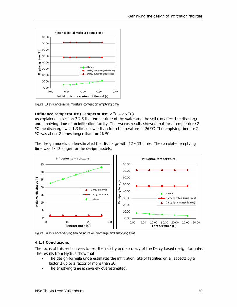
Initial moisture content (Initial moisture content: 0.08 - 0.32) For the initial moisture content θi only the emptying time could be modelled with Hydrus. The maximum discharge could not be modelled. The model runs were done from the minimum moisture content of the soil (residual moisture content) θr = 0.065 till near the saturated moisture content θs = 0.41. The results showed an increasing emptying time for increasing initial moisture content. However the difference between low and high moisture content was only a factor 2.5. The design models overestimated the emptying time 5-12 times.
Influence clogged bottom
0
5
10
15
20
25
30
35
0 5 10 15Clogged bottom ratio [-]
Rel
ativ
e di
scha
rge
[-]
Darcy dynamic
Darcy constantHydrus
Hydrus fully clogged
Darcy constant bot
Darcy dynamic bot
Influence clogged bottom
0.00
10.00
20.00
30.00
40.00
50.00
60.00
70.00
80.00
0.00 5.00 10.00 15.00
Clogged bottom ratio [-]
Em
pty
ing
tim
e [h
]
Darcy constant Darcy dynamic Hydrus Hydrus fully cloggedDarcy constant botDarcy dynamic bot
Rethinking the design of infiltration facilities
MSc Thesis Leon Valkenburg 20
Figure 13 Influence initial moisture content on emptying time
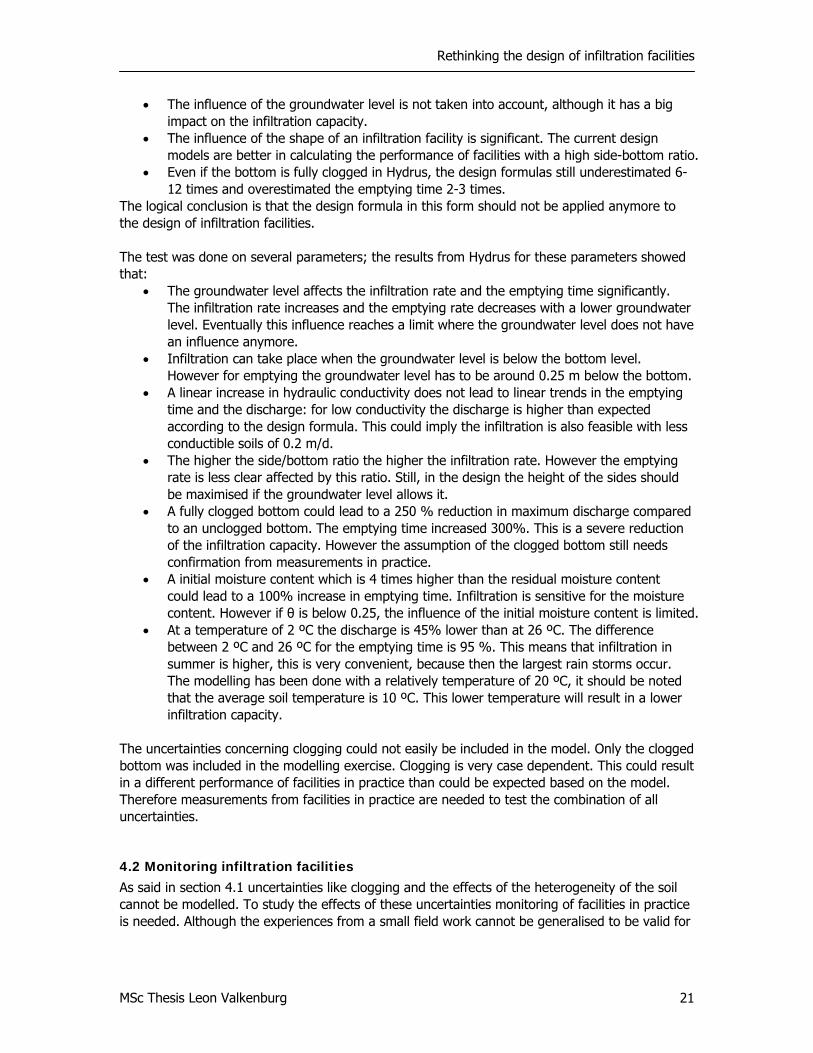
Influence temperature (Temperature: 2 oC – 26 oC) As explained in section 2.2.5 the temperature of the water and the soil can affect the discharge and emptying time of an infiltration facility. The Hydrus results showed that for a temperature 2 ºC the discharge was 1.3 times lower than for a temperature of 26 ºC. The emptying time for 2 ºC was about 2 times longer than for 26 ºC. The design models underestimated the discharge with 12 - 33 times. The calculated emptying time was 5- 12 longer for the design models.
Figure 14 Influence varying temperature on discharge and emptying time
4.1.4 Conclusions The focus of this section was to test the validity and accuracy of the Darcy based design formulas. The results from Hydrus show that:
• The design formula underestimates the infiltration rate of facilities on all aspects by a factor 2 up to a factor of more than 30.
• The emptying time is severely overestimated.
Influence initial moisture conditions
0.00
10.00
20.00
30.00
40.00
50.00
60.00
70.00
80.00
0.00 0.10 0.20 0.30 0.40
Initial moisture content of the soil [-]
Empt
ying
tim
e [h
]
Hydrus Darcy constant (guidelines)Darcy dynamic (guidelines)
Influence temperature
0
5
10
15
20
25
30
35
0 10 20 30Temperature [C]
Rel
ativ
e di
scha
rge
[-]
Darcy dynamic
Darcy constant
Hydrus
Influence temperature
0.00
10.00
20.00
30.00
40.00
50.00
60.00
70.00
80.00
0.00 5.00 10.00 15.00 20.00 25.00 30.00Temperature [C]
Empt
ying
tim
e [h
]
Hydrus
Darcy constant (guidelines)
Darcy dynamic (guidelines)
Rethinking the design of infiltration facilities
MSc Thesis Leon Valkenburg 21
• The influence of the groundwater level is not taken into account, although it has a big impact on the infiltration capacity.
• The influence of the shape of an infiltration facility is significant. The current design models are better in calculating the performance of facilities with a high side-bottom ratio.
• Even if the bottom is fully clogged in Hydrus, the design formulas still underestimated 6-12 times and overestimated the emptying time 2-3 times.
The logical conclusion is that the design formula in this form should not be applied anymore to the design of infiltration facilities. The test was done on several parameters; the results from Hydrus for these parameters showed that:
• The groundwater level affects the infiltration rate and the emptying time significantly. The infiltration rate increases and the emptying rate decreases with a lower groundwater level. Eventually this influence reaches a limit where the groundwater level does not have an influence anymore.
• Infiltration can take place when the groundwater level is below the bottom level. However for emptying the groundwater level has to be around 0.25 m below the bottom.
• A linear increase in hydraulic conductivity does not lead to linear trends in the emptying time and the discharge: for low conductivity the discharge is higher than expected according to the design formula. This could imply the infiltration is also feasible with less conductible soils of 0.2 m/d.
• The higher the side/bottom ratio the higher the infiltration rate. However the emptying rate is less clear affected by this ratio. Still, in the design the height of the sides should be maximised if the groundwater level allows it.
• A fully clogged bottom could lead to a 250 % reduction in maximum discharge compared to an unclogged bottom. The emptying time increased 300%. This is a severe reduction of the infiltration capacity. However the assumption of the clogged bottom still needs confirmation from measurements in practice.
• A initial moisture content which is 4 times higher than the residual moisture content could lead to a 100% increase in emptying time. Infiltration is sensitive for the moisture content. However if θ is below 0.25, the influence of the initial moisture content is limited.
• At a temperature of 2 ºC the discharge is 45% lower than at 26 ºC. The difference between 2 ºC and 26 ºC for the emptying time is 95 %. This means that infiltration in summer is higher, this is very convenient, because then the largest rain storms occur. The modelling has been done with a relatively temperature of 20 ºC, it should be noted that the average soil temperature is 10 ºC. This lower temperature will result in a lower infiltration capacity.
The uncertainties concerning clogging could not easily be included in the model. Only the clogged bottom was included in the modelling exercise. Clogging is very case dependent. This could result in a different performance of facilities in practice than could be expected based on the model. Therefore measurements from facilities in practice are needed to test the combination of all uncertainties.
4.2 Monitoring infiltration facilities As said in section 4.1 uncertainties like clogging and the effects of the heterogeneity of the soil cannot be modelled. To study the effects of these uncertainties monitoring of facilities in practice is needed. Although the experiences from a small field work cannot be generalised to be valid for
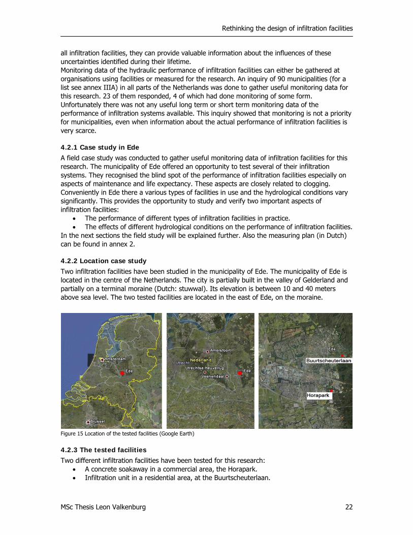
Rethinking the design of infiltration facilities
MSc Thesis Leon Valkenburg 22
all infiltration facilities, they can provide valuable information about the influences of these uncertainties identified during their lifetime. Monitoring data of the hydraulic performance of infiltration facilities can either be gathered at organisations using facilities or measured for the research. An inquiry of 90 municipalities (for a list see annex IIIA) in all parts of the Netherlands was done to gather useful monitoring data for this research. 23 of them responded, 4 of which had done monitoring of some form. Unfortunately there was not any useful long term or short term monitoring data of the performance of infiltration systems available. This inquiry showed that monitoring is not a priority for municipalities, even when information about the actual performance of infiltration facilities is very scarce.
4.2.1 Case study in Ede A field case study was conducted to gather useful monitoring data of infiltration facilities for this research. The municipality of Ede offered an opportunity to test several of their infiltration systems. They recognised the blind spot of the performance of infiltration facilities especially on aspects of maintenance and life expectancy. These aspects are closely related to clogging. Conveniently in Ede there a various types of facilities in use and the hydrological conditions vary significantly. This provides the opportunity to study and verify two important aspects of infiltration facilities:
• The performance of different types of infiltration facilities in practice. • The effects of different hydrological conditions on the performance of infiltration facilities.
In the next sections the field study will be explained further. Also the measuring plan (in Dutch) can be found in annex 2.
4.2.2 Location case study Two infiltration facilities have been studied in the municipality of Ede. The municipality of Ede is located in the centre of the Netherlands. The city is partially built in the valley of Gelderland and partially on a terminal moraine (Dutch: stuwwal). Its elevation is between 10 and 40 meters above sea level. The two tested facilities are located in the east of Ede, on the moraine.
Figure 15 Location of the tested facilities (Google Earth)
4.2.3 The tested facilities Two different infiltration facilities have been tested for this research:
• A concrete soakaway in a commercial area, the Horapark. • Infiltration unit in a residential area, at the Buurtscheuterlaan.
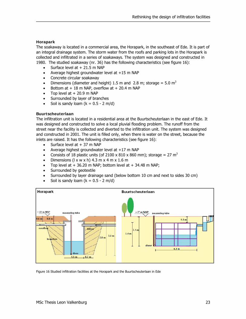
Rethinking the design of infiltration facilities
MSc Thesis Leon Valkenburg 23
Horapark The soakaway is located in a commercial area, the Horapark, in the southeast of Ede. It is part of an integral drainage system. The storm water from the roofs and parking lots in the Horapark is collected and infiltrated in a series of soakaways. The system was designed and constructed in 1980. The studied soakaway (nr. 36) has the following characteristics (see figure 16):
• Surface level at + 21.5 m NAP • Average highest groundwater level at +15 m NAP • Concrete circular soakaway • Dimensions (diameter and height) 1.5 m and 2.8 m; storage = 5.0 m3 • Bottom at + 18 m NAP, overflow at + 20.4 m NAP • Top level at + 20.9 m NAP • Surrounded by layer of branches • Soil is sandy loam (k = 0.5 - 2 m/d)
Buurtscheuterlaan The infiltration unit is located in a residential area at the Buurtscheuterlaan in the east of Ede. It was designed and constructed to solve a local pluvial flooding problem. The runoff from the street near the facility is collected and diverted to the infiltration unit. The system was designed and constructed in 2001. The unit is filled only, when there is water on the street, because the inlets are raised. It has the following characteristics (see figure 16):
• Surface level at + 37 m NAP • Average highest groundwater level at +17 m NAP • Consists of 18 plastic units (of 2100 x 810 x 860 mm); storage = 27 m3 • Dimensions (l x w x h) 4.3 m x 4 m x 1.6 m • Top level at + 36.20 m NAP; bottom level at + 34.48 m NAP; • Surrounded by geotextile • Surrounded by layer drainage sand (below bottom 10 cm and next to sides 30 cm) • Soil is sandy loam (k = 0.5 - 2 m/d)
Figure 16 Studied infiltration facilities at the Horapark and the Buurtscheuterlaan in Ede
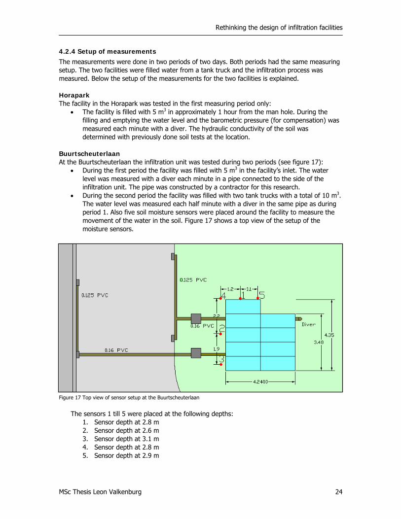
Rethinking the design of infiltration facilities
MSc Thesis Leon Valkenburg 24
4.2.4 Setup of measurements The measurements were done in two periods of two days. Both periods had the same measuring setup. The two facilities were filled water from a tank truck and the infiltration process was measured. Below the setup of the measurements for the two facilities is explained. Horapark The facility in the Horapark was tested in the first measuring period only:
• The facility is filled with 5 m3 in approximately 1 hour from the man hole. During the filling and emptying the water level and the barometric pressure (for compensation) was measured each minute with a diver. The hydraulic conductivity of the soil was determined with previously done soil tests at the location.
Buurtscheuterlaan At the Buurtscheuterlaan the infiltration unit was tested during two periods (see figure 17):
• During the first period the facility was filled with 5 m3 in the facility’s inlet. The water level was measured with a diver each minute in a pipe connected to the side of the infiltration unit. The pipe was constructed by a contractor for this research.
• During the second period the facility was filled with two tank trucks with a total of 10 m3. The water level was measured each half minute with a diver in the same pipe as during period 1. Also five soil moisture sensors were placed around the facility to measure the movement of the water in the soil. Figure 17 shows a top view of the setup of the moisture sensors.
Figure 17 Top view of sensor setup at the Buurtscheuterlaan
The sensors 1 till 5 were placed at the following depths:
1. Sensor depth at 2.8 m 2. Sensor depth at 2.6 m 3. Sensor depth at 3.1 m 4. Sensor depth at 2.8 m 5. Sensor depth at 2.9 m
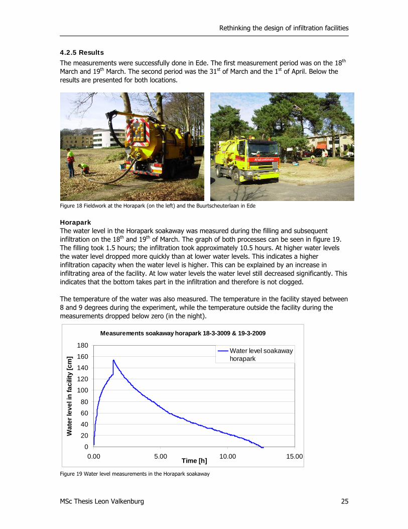
Rethinking the design of infiltration facilities
MSc Thesis Leon Valkenburg 25
4.2.5 Results The measurements were successfully done in Ede. The first measurement period was on the 18th March and 19th March. The second period was the 31st of March and the 1st of April. Below the results are presented for both locations.
Figure 18 Fieldwork at the Horapark (on the left) and the Buurtscheuterlaan in Ede
Horapark The water level in the Horapark soakaway was measured during the filling and subsequent infiltration on the 18th and 19th of March. The graph of both processes can be seen in figure 19. The filling took 1.5 hours; the infiltration took approximately 10.5 hours. At higher water levels the water level dropped more quickly than at lower water levels. This indicates a higher infiltration capacity when the water level is higher. This can be explained by an increase in infiltrating area of the facility. At low water levels the water level still decreased significantly. This indicates that the bottom takes part in the infiltration and therefore is not clogged. The temperature of the water was also measured. The temperature in the facility stayed between 8 and 9 degrees during the experiment, while the temperature outside the facility during the measurements dropped below zero (in the night).
Figure 19 Water level measurements in the Horapark soakaway
Measurements soakaway horapark 18-3-3009 & 19-3-2009
0
20
40
60
80
100
120
140
160
180
0.00 5.00 10.00 15.00Time [h]
Wat
er le
vel i
n fa
cilit
y [c
m]
Water level soakawayhorapark
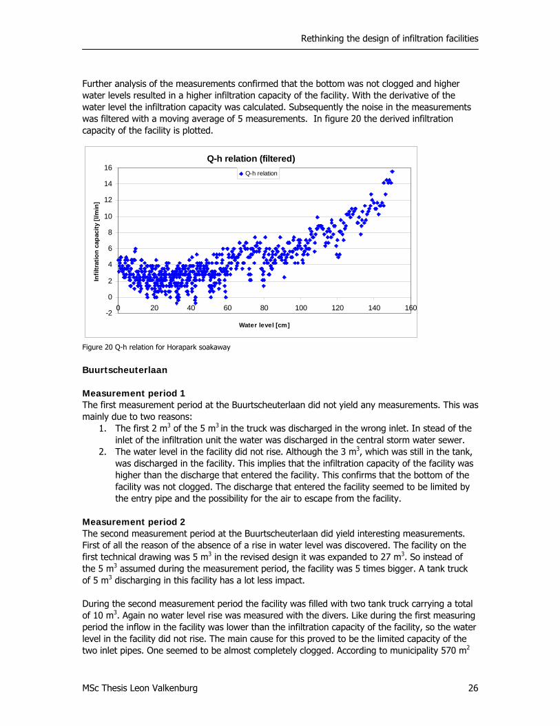
Rethinking the design of infiltration facilities
MSc Thesis Leon Valkenburg 26
Further analysis of the measurements confirmed that the bottom was not clogged and higher water levels resulted in a higher infiltration capacity of the facility. With the derivative of the water level the infiltration capacity was calculated. Subsequently the noise in the measurements was filtered with a moving average of 5 measurements. In figure 20 the derived infiltration capacity of the facility is plotted.
Figure 20 Q-h relation for Horapark soakaway
Buurtscheuterlaan Measurement period 1 The first measurement period at the Buurtscheuterlaan did not yield any measurements. This was mainly due to two reasons:
1. The first 2 m3 of the 5 m3 in the truck was discharged in the wrong inlet. In stead of the inlet of the infiltration unit the water was discharged in the central storm water sewer.
2. The water level in the facility did not rise. Although the 3 m3, which was still in the tank, was discharged in the facility. This implies that the infiltration capacity of the facility was higher than the discharge that entered the facility. This confirms that the bottom of the facility was not clogged. The discharge that entered the facility seemed to be limited by the entry pipe and the possibility for the air to escape from the facility.
Measurement period 2 The second measurement period at the Buurtscheuterlaan did yield interesting measurements. First of all the reason of the absence of a rise in water level was discovered. The facility on the first technical drawing was 5 m3 in the revised design it was expanded to 27 m3. So instead of the 5 m3 assumed during the measurement period, the facility was 5 times bigger. A tank truck of 5 m3 discharging in this facility has a lot less impact. During the second measurement period the facility was filled with two tank truck carrying a total of 10 m3. Again no water level rise was measured with the divers. Like during the first measuring period the inflow in the facility was lower than the infiltration capacity of the facility, so the water level in the facility did not rise. The main cause for this proved to be the limited capacity of the two inlet pipes. One seemed to be almost completely clogged. According to municipality 570 m2
Q-h relation (filtered)
-2
0
2
4
6
8
10
12
14
16
0 20 40 60 80 100 120 140 160
Water level [cm]
Infil
trat
ion
capa
city
[l/m
in]
Q-h relation
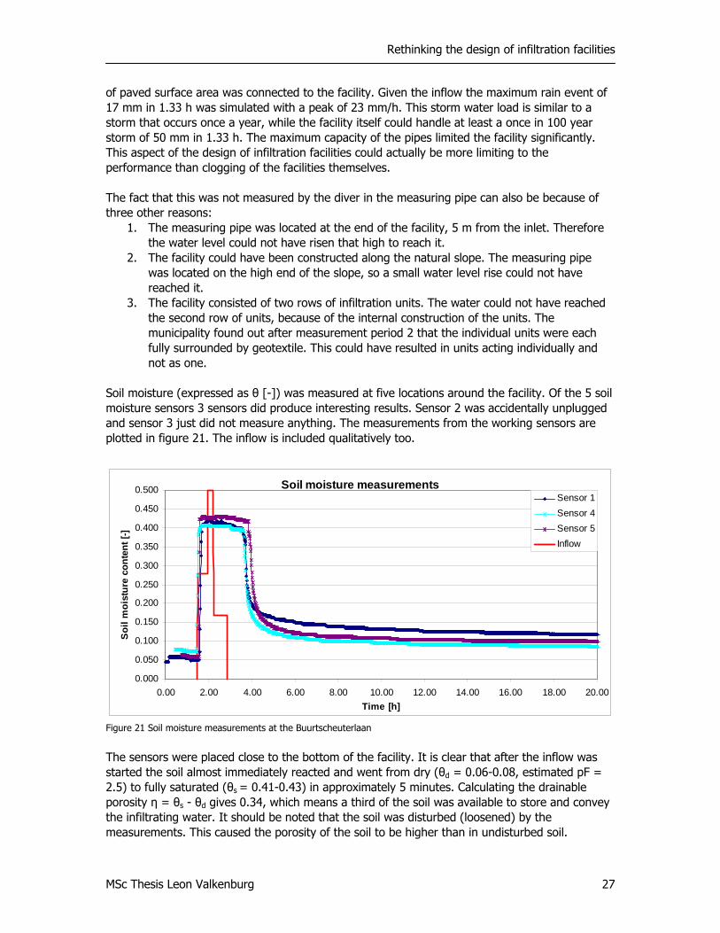
Rethinking the design of infiltration facilities
MSc Thesis Leon Valkenburg 27
of paved surface area was connected to the facility. Given the inflow the maximum rain event of 17 mm in 1.33 h was simulated with a peak of 23 mm/h. This storm water load is similar to a storm that occurs once a year, while the facility itself could handle at least a once in 100 year storm of 50 mm in 1.33 h. The maximum capacity of the pipes limited the facility significantly. This aspect of the design of infiltration facilities could actually be more limiting to the performance than clogging of the facilities themselves. The fact that this was not measured by the diver in the measuring pipe can also be because of three other reasons:
1. The measuring pipe was located at the end of the facility, 5 m from the inlet. Therefore the water level could not have risen that high to reach it.
2. The facility could have been constructed along the natural slope. The measuring pipe was located on the high end of the slope, so a small water level rise could not have reached it.
3. The facility consisted of two rows of infiltration units. The water could not have reached the second row of units, because of the internal construction of the units. The municipality found out after measurement period 2 that the individual units were each fully surrounded by geotextile. This could have resulted in units acting individually and not as one.
Soil moisture (expressed as θ [-]) was measured at five locations around the facility. Of the 5 soil moisture sensors 3 sensors did produce interesting results. Sensor 2 was accidentally unplugged and sensor 3 just did not measure anything. The measurements from the working sensors are plotted in figure 21. The inflow is included qualitatively too.
Figure 21 Soil moisture measurements at the Buurtscheuterlaan
The sensors were placed close to the bottom of the facility. It is clear that after the inflow was started the soil almost immediately reacted and went from dry (θd = 0.06-0.08, estimated pF = 2.5) to fully saturated (θs = 0.41-0.43) in approximately 5 minutes. Calculating the drainable porosity η = θs - θd gives 0.34, which means a third of the soil was available to store and convey the infiltrating water. It should be noted that the soil was disturbed (loosened) by the measurements. This caused the porosity of the soil to be higher than in undisturbed soil.
Soil moisture measurements
0.000
0.050
0.100
0.150
0.200
0.250
0.300
0.350
0.400
0.450
0.500
0.00 2.00 4.00 6.00 8.00 10.00 12.00 14.00 16.00 18.00 20.00Time [h]
Soi
l moi
stur
e co
nten
t [-]
Sensor 1Sensor 4Sensor 5Inflow

Rethinking the design of infiltration facilities
MSc Thesis Leon Valkenburg 28
After the inflow was stopped the soil was fully saturated for another 1.5 hours before an exponential decrease in moisture content could begin (towards a pF of 2). This could indicate that part of the storage of the facility was actually filled, because infiltration was still taking place when the inflow was stopped.
4.2.6 Conclusions Based on the measurements the following conclusions can be drawn:
• The effects of clogging in both facilities were very limited. The bottom areas of both facilities were clearly not clogged.
• The infiltration capacity of both facilities was much larger than assumed in the design. • It was impossible to fill the facility at the Buurtscheuterlaan completely by a tank truck or
an extreme rain event, because the capacity of the inlet pipes was too small. The design of inlets and overflows is an aspect deserving more attention in the design.
• The measurements in the facility at the Horapark showed that high water levels result in high infiltration capacity.
The two studied facilities in Ede cannot be considered as completely generic for other infiltration facilities. The results of the measurement should be used considering the specific conditions at the facilities. The geohydrologic location of the facilities is favourable for infiltration: the groundwater level was too low to affect the performance and the hydraulic conductivity of the soil was high. Also the usual storm water load on the facilities is beneficial for their performance. The soakaway at the Horapark is part of a series of soakaways, and as it is not the first in line, the water it receives is low on sediments. Water enters the infiltration unit at the Buurtscheuterlaan only when a significant amount of water is on the street. This happens perhaps 10 times per year; this is much less than a facility directly connected to a roof. The smaller storm water load could have resulted in less clogging.
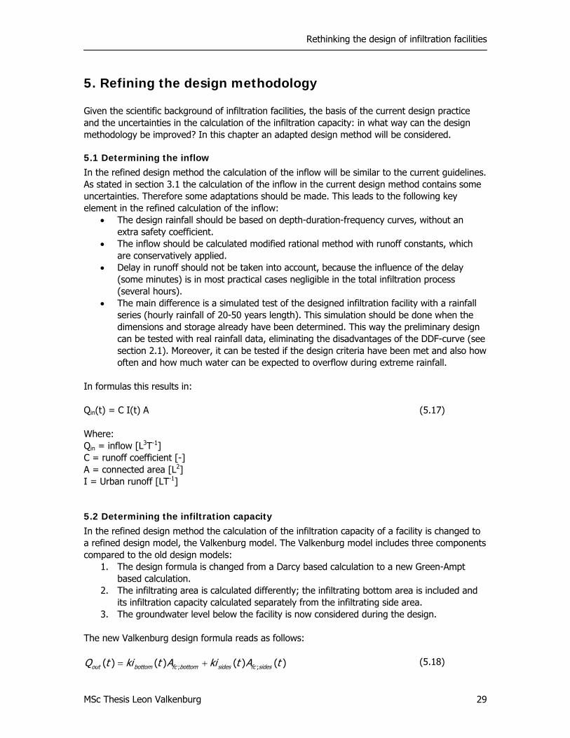
Rethinking the design of infiltration facilities
MSc Thesis Leon Valkenburg 29
; ;( ) ( ) ( ) ( )out bottom fc bottom sides fc sidesQ t ki t A ki t A t= +
5. Refining the design methodology Given the scientific background of infiltration facilities, the basis of the current design practice and the uncertainties in the calculation of the infiltration capacity: in what way can the design methodology be improved? In this chapter an adapted design method will be considered.
5.1 Determining the inflow In the refined design method the calculation of the inflow will be similar to the current guidelines. As stated in section 3.1 the calculation of the inflow in the current design method contains some uncertainties. Therefore some adaptations should be made. This leads to the following key element in the refined calculation of the inflow:
• The design rainfall should be based on depth-duration-frequency curves, without an extra safety coefficient.
• The inflow should be calculated modified rational method with runoff constants, which are conservatively applied.
• Delay in runoff should not be taken into account, because the influence of the delay (some minutes) is in most practical cases negligible in the total infiltration process (several hours).
• The main difference is a simulated test of the designed infiltration facility with a rainfall series (hourly rainfall of 20-50 years length). This simulation should be done when the dimensions and storage already have been determined. This way the preliminary design can be tested with real rainfall data, eliminating the disadvantages of the DDF-curve (see section 2.1). Moreover, it can be tested if the design criteria have been met and also how often and how much water can be expected to overflow during extreme rainfall.
In formulas this results in: Qin(t) = C I(t) A (5.17) Where: Qin = inflow [L3T-1] C = runoff coefficient [-] A = connected area [L2] I = Urban runoff [LT-1]
5.2 Determining the infiltration capacity In the refined design method the calculation of the infiltration capacity of a facility is changed to a refined design model, the Valkenburg model. The Valkenburg model includes three components compared to the old design models:
1. The design formula is changed from a Darcy based calculation to a new Green-Ampt based calculation.
2. The infiltrating area is calculated differently; the infiltrating bottom area is included and its infiltration capacity calculated separately from the infiltrating side area.
3. The groundwater level below the facility is now considered during the design. The new Valkenburg design formula reads as follows:
(5.18)
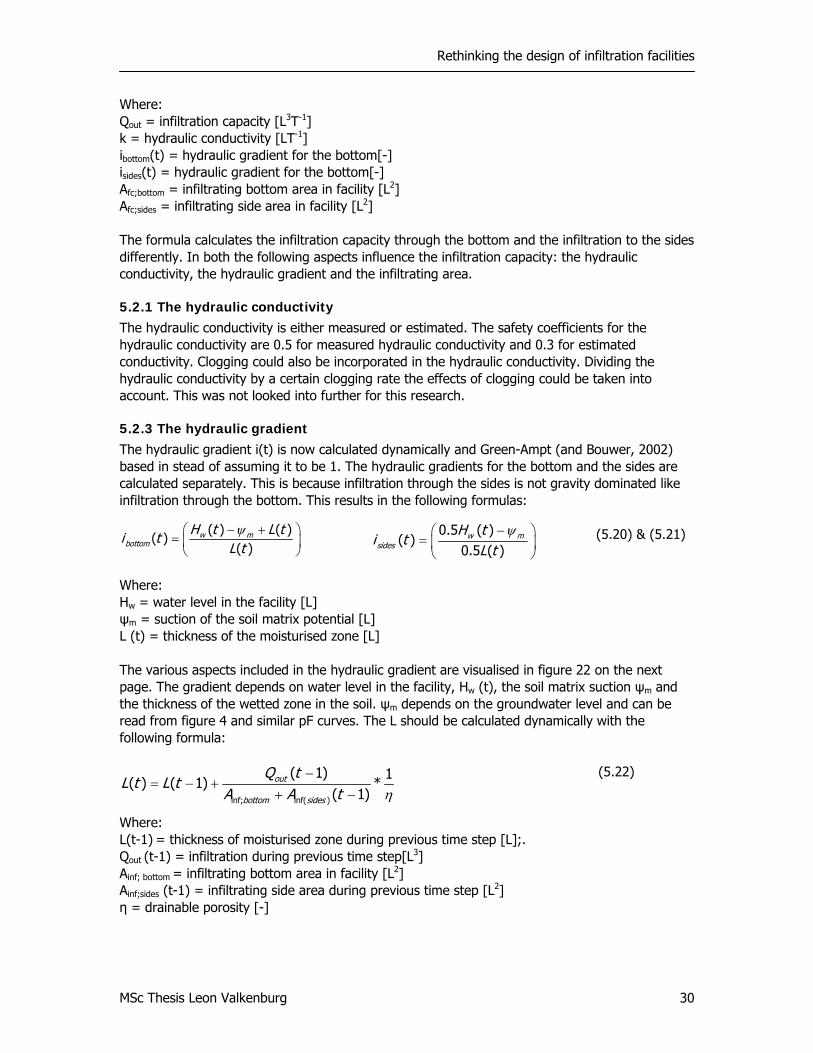
Rethinking the design of infiltration facilities
MSc Thesis Leon Valkenburg 30
( ) ( )( )
( )w m
bottomH t L ti t
L tψ− +⎛ ⎞
= ⎜ ⎟⎝ ⎠
inf; inf( )
( 1) 1( ) ( 1) *
( 1)out
bottom sides
Q tL t L t
A A t η−
= − ++ −
0.5 ( )( )
0.5 ( )w m
sides
H ti t
L tψ−⎛ ⎞
= ⎜ ⎟⎝ ⎠
Where: Qout = infiltration capacity [L3T-1] k = hydraulic conductivity [LT-1] ibottom(t) = hydraulic gradient for the bottom[-] isides(t) = hydraulic gradient for the bottom[-] Afc;bottom = infiltrating bottom area in facility [L2] Afc;sides = infiltrating side area in facility [L2] The formula calculates the infiltration capacity through the bottom and the infiltration to the sides differently. In both the following aspects influence the infiltration capacity: the hydraulic conductivity, the hydraulic gradient and the infiltrating area.
5.2.1 The hydraulic conductivity The hydraulic conductivity is either measured or estimated. The safety coefficients for the hydraulic conductivity are 0.5 for measured hydraulic conductivity and 0.3 for estimated conductivity. Clogging could also be incorporated in the hydraulic conductivity. Dividing the hydraulic conductivity by a certain clogging rate the effects of clogging could be taken into account. This was not looked into further for this research.
5.2.3 The hydraulic gradient The hydraulic gradient i(t) is now calculated dynamically and Green-Ampt (and Bouwer, 2002) based in stead of assuming it to be 1. The hydraulic gradients for the bottom and the sides are calculated separately. This is because infiltration through the sides is not gravity dominated like infiltration through the bottom. This results in the following formulas:
(5.20) & (5.21)
Where: Hw = water level in the facility [L] ψm = suction of the soil matrix potential [L] L (t) = thickness of the moisturised zone [L] The various aspects included in the hydraulic gradient are visualised in figure 22 on the next page. The gradient depends on water level in the facility, Hw (t), the soil matrix suction ψm and the thickness of the wetted zone in the soil. ψm depends on the groundwater level and can be read from figure 4 and similar pF curves. The L should be calculated dynamically with the following formula: (5.22) Where: L(t-1) = thickness of moisturised zone during previous time step [L];. Qout (t-1) = infiltration during previous time step[L3]
Ainf; bottom = infiltrating bottom area in facility [L2] Ainf;sides (t-1) = infiltrating side area during previous time step [L2] η = drainable porosity [-]
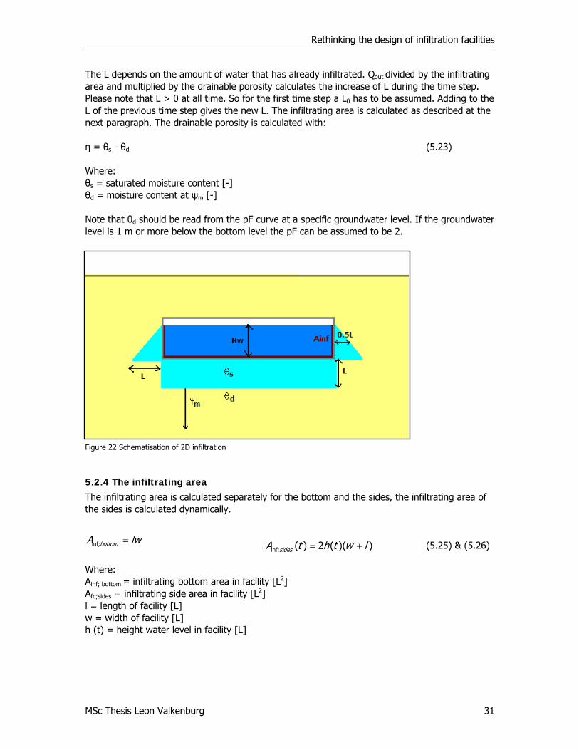
Rethinking the design of infiltration facilities
MSc Thesis Leon Valkenburg 31
inf;bottomA lw=inf; ( ) 2 ( )( )sidesA t h t w l= +
The L depends on the amount of water that has already infiltrated. Qout divided by the infiltrating area and multiplied by the drainable porosity calculates the increase of L during the time step. Please note that L > 0 at all time. So for the first time step a L0 has to be assumed. Adding to the L of the previous time step gives the new L. The infiltrating area is calculated as described at the next paragraph. The drainable porosity is calculated with: η = θs - θd (5.23) Where: θs = saturated moisture content [-] θd = moisture content at ψm [-] Note that θd should be read from the pF curve at a specific groundwater level. If the groundwater level is 1 m or more below the bottom level the pF can be assumed to be 2.
Figure 22 Schematisation of 2D infiltration
5.2.4 The infiltrating area The infiltrating area is calculated separately for the bottom and the sides, the infiltrating area of the sides is calculated dynamically.
(5.25) & (5.26) Where: Ainf; bottom = infiltrating bottom area in facility [L2] Afc;sides = infiltrating side area in facility [L2] l = length of facility [L] w = width of facility [L] h (t) = height water level in facility [L]
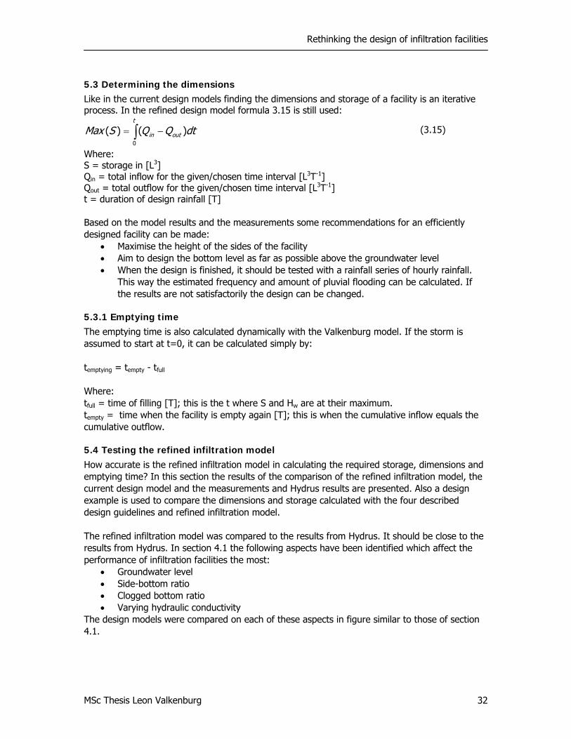
Rethinking the design of infiltration facilities
MSc Thesis Leon Valkenburg 32
5.3 Determining the dimensions Like in the current design models finding the dimensions and storage of a facility is an iterative process. In the refined design model formula 3.15 is still used:
0
( ) ( )t
in outMax S Q Q dt= −∫ (3.15)
Where: S = storage in [L3] Qin = total inflow for the given/chosen time interval [L3T-1] Qout = total outflow for the given/chosen time interval [L3T-1] t = duration of design rainfall [T] Based on the model results and the measurements some recommendations for an efficiently designed facility can be made:
• Maximise the height of the sides of the facility • Aim to design the bottom level as far as possible above the groundwater level • When the design is finished, it should be tested with a rainfall series of hourly rainfall.
This way the estimated frequency and amount of pluvial flooding can be calculated. If the results are not satisfactorily the design can be changed.
5.3.1 Emptying time The emptying time is also calculated dynamically with the Valkenburg model. If the storm is assumed to start at t=0, it can be calculated simply by: temptying = tempty - tfull
Where: tfull = time of filling [T]; this is the t where S and Hw are at their maximum. tempty = time when the facility is empty again [T]; this is when the cumulative inflow equals the cumulative outflow.
5.4 Testing the refined infiltration model How accurate is the refined infiltration model in calculating the required storage, dimensions and emptying time? In this section the results of the comparison of the refined infiltration model, the current design model and the measurements and Hydrus results are presented. Also a design example is used to compare the dimensions and storage calculated with the four described design guidelines and refined infiltration model. The refined infiltration model was compared to the results from Hydrus. It should be close to the results from Hydrus. In section 4.1 the following aspects have been identified which affect the performance of infiltration facilities the most:
• Groundwater level • Side-bottom ratio • Clogged bottom ratio • Varying hydraulic conductivity
The design models were compared on each of these aspects in figure similar to those of section 4.1.
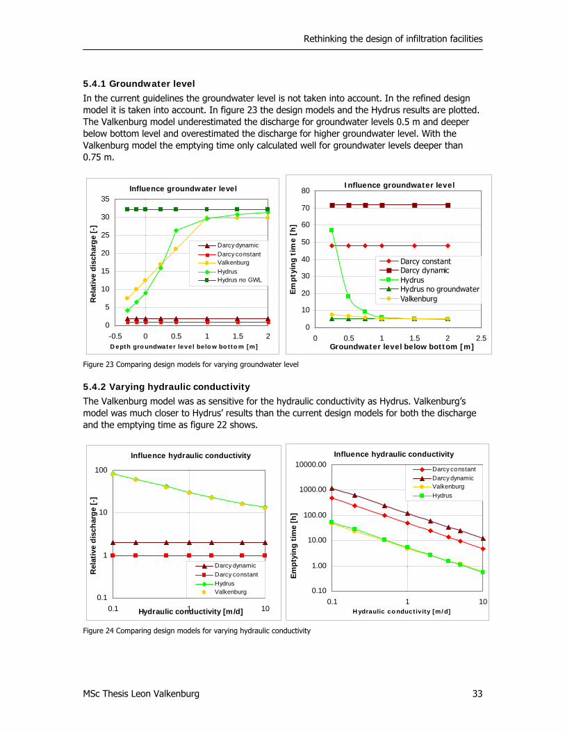
Rethinking the design of infiltration facilities
MSc Thesis Leon Valkenburg 33
5.4.1 Groundwater level In the current guidelines the groundwater level is not taken into account. In the refined design model it is taken into account. In figure 23 the design models and the Hydrus results are plotted. The Valkenburg model underestimated the discharge for groundwater levels 0.5 m and deeper below bottom level and overestimated the discharge for higher groundwater level. With the Valkenburg model the emptying time only calculated well for groundwater levels deeper than 0.75 m.
Figure 23 Comparing design models for varying groundwater level
5.4.2 Varying hydraulic conductivity The Valkenburg model was as sensitive for the hydraulic conductivity as Hydrus. Valkenburg’s model was much closer to Hydrus’ results than the current design models for both the discharge and the emptying time as figure 22 shows.
Figure 24 Comparing design models for varying hydraulic conductivity
Influence hydraulic conductivity
0.1
1
10
100
0.1 1 10Hydraulic conductivity [m/d]
Rel
ativ
e di
scha
rge
[-]
Darcy dynamicDarcy constantHydrusValkenburg
Influence hydraulic conductivity
0.10
1.00
10.00
100.00
1000.00
10000.00
0.1 1 10H ydraulic co nduct iv ity [m/ d]
Empt
ying
tim
e [h
]
Darcy constant Darcy dynamic ValkenburgHydrus
Influence groundwater level
0
5
10
15
20
25
30
35
-0.5 0 0.5 1 1.5 2D epth gro undwater level belo w bo tto m [m]
Rel
ativ
e di
scha
rge
[-]
Darcy dynamicDarcy constantValkenburgHydrusHydrus no GWL
Influence groundwater level
0
10
20
30
40
50
60
70
80
0 0.5 1 1.5 2 2.5Groundwater level below bottom [m]
Empt
yin
g ti
me
[h
]
Darcy constant Darcy dynamic Hydrus Hydrus no groundwaterValkenburg
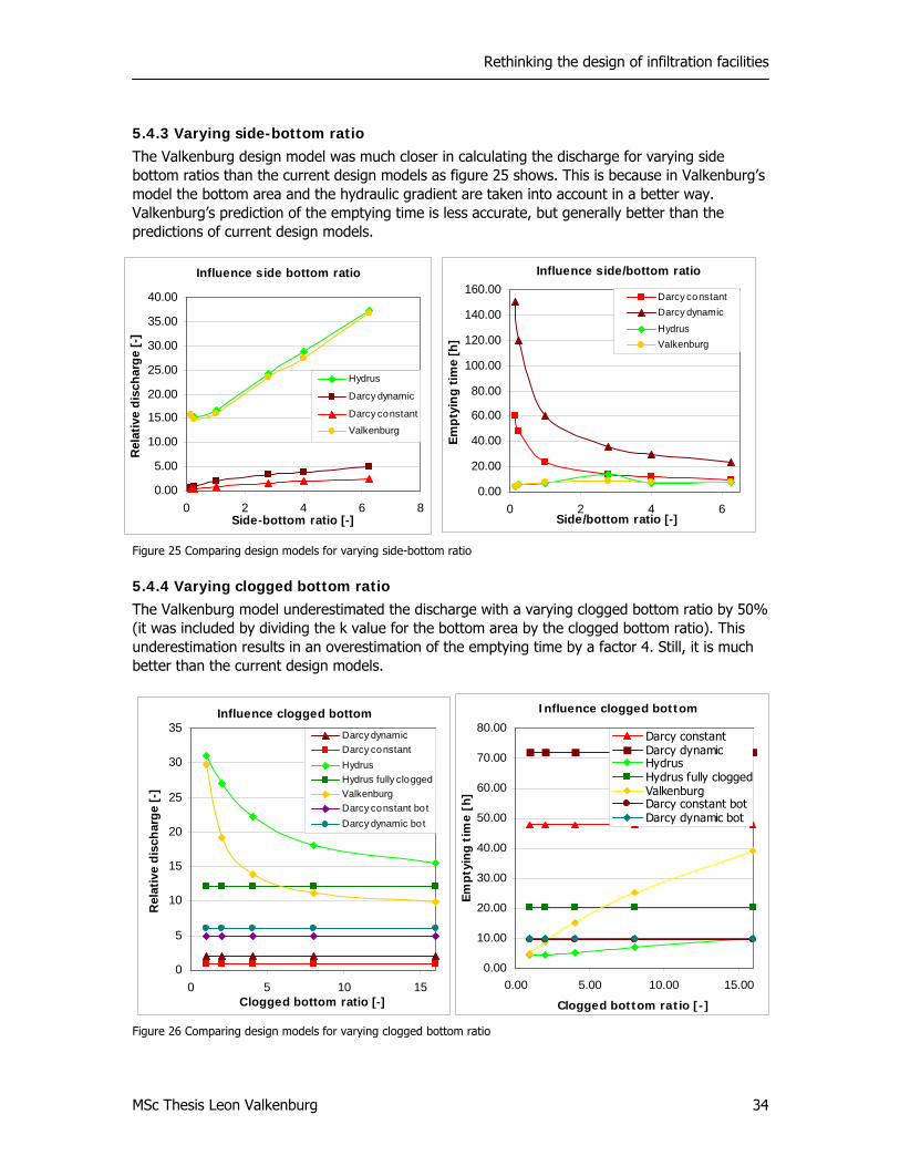
Rethinking the design of infiltration facilities
MSc Thesis Leon Valkenburg 34
5.4.3 Varying side-bottom ratio The Valkenburg design model was much closer in calculating the discharge for varying side bottom ratios than the current design models as figure 25 shows. This is because in Valkenburg’s model the bottom area and the hydraulic gradient are taken into account in a better way. Valkenburg’s prediction of the emptying time is less accurate, but generally better than the predictions of current design models.
Figure 25 Comparing design models for varying side-bottom ratio
5.4.4 Varying clogged bottom ratio The Valkenburg model underestimated the discharge with a varying clogged bottom ratio by 50% (it was included by dividing the k value for the bottom area by the clogged bottom ratio). This underestimation results in an overestimation of the emptying time by a factor 4. Still, it is much better than the current design models.
Figure 26 Comparing design models for varying clogged bottom ratio
Influence side/bottom ratio
0.00
20.00
40.00
60.00
80.00
100.00
120.00
140.00
160.00
0 2 4 6Side/bottom ratio [-]
Empt
ying
tim
e [h
]
Darcy constant Darcy dynamic Hydrus Valkenburg
Influence side bottom ratio
0.00
5.00
10.00
15.00
20.00
25.00
30.00
35.00
40.00
0 2 4 6 8Side-bottom ratio [-]
Rel
ativ
e di
scha
rge
[-]
Hydrus
Darcy dynamic
Darcy constant
Valkenburg
Influence clogged bottom
0
5
10
15
20
25
30
35
0 5 10 15Clogged bottom ratio [-]
Rel
ativ
e di
scha
rge
[-]
Darcy dynamicDarcy constantHydrusHydrus fully cloggedValkenburgDarcy constant botDarcy dynamic bot
Influence clogged bottom
0.00
10.00
20.00
30.00
40.00
50.00
60.00
70.00
80.00
0.00 5.00 10.00 15.00
Clogged bottom ratio [-]
Em
pty
ing
tim
e [h
]
Darcy constant Darcy dynamic Hydrus Hydrus fully cloggedValkenburgDarcy constant botDarcy dynamic bot
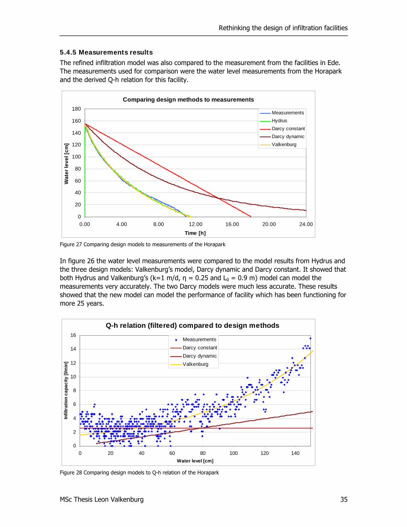
Rethinking the design of infiltration facilities
MSc Thesis Leon Valkenburg 35
5.4.5 Measurements results The refined infiltration model was also compared to the measurement from the facilities in Ede. The measurements used for comparison were the water level measurements from the Horapark and the derived Q-h relation for this facility.
Figure 27 Comparing design models to measurements of the Horapark
In figure 26 the water level measurements were compared to the model results from Hydrus and the three design models: Valkenburg’s model, Darcy dynamic and Darcy constant. It showed that both Hydrus and Valkenburg’s (k=1 m/d, η = 0.25 and L0 = 0.9 m) model can model the measurements very accurately. The two Darcy models were much less accurate. These results showed that the new model can model the performance of facility which has been functioning for more 25 years.
Figure 28 Comparing design models to Q-h relation of the Horapark
Comparing design methods to measurements
0
20
40
60
80
100
120
140
160
180
0.00 4.00 8.00 12.00 16.00 20.00 24.00
Time [h]
Wat
er le
vel [
cm]
MeasurementsHydrusDarcy constantDarcy dynamicValkenburg
Q-h relation (filtered) compared to design methods
0
2
4
6
8
10
12
14
16
0 20 40 60 80 100 120 140Water level [cm]
Infil
trat
ion
capa
city
[l/m
in]
MeasurementsDarcy constantDarcy dynamicValkenburg
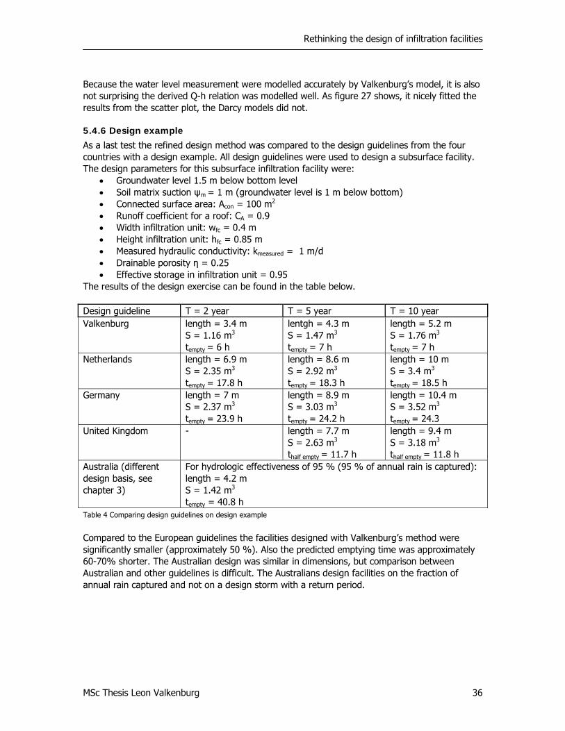
Rethinking the design of infiltration facilities
MSc Thesis Leon Valkenburg 36
Because the water level measurement were modelled accurately by Valkenburg’s model, it is also not surprising the derived Q-h relation was modelled well. As figure 27 shows, it nicely fitted the results from the scatter plot, the Darcy models did not.
5.4.6 Design example As a last test the refined design method was compared to the design guidelines from the four countries with a design example. All design guidelines were used to design a subsurface facility. The design parameters for this subsurface infiltration facility were:
• Groundwater level 1.5 m below bottom level • Soil matrix suction ψm = 1 m (groundwater level is 1 m below bottom) • Connected surface area: Acon = 100 m2 • Runoff coefficient for a roof: CA = 0.9 • Width infiltration unit: wfc = 0.4 m • Height infiltration unit: hfc = 0.85 m • Measured hydraulic conductivity: kmeasured = 1 m/d • Drainable porosity η = 0.25 • Effective storage in infiltration unit = 0.95
The results of the design exercise can be found in the table below. Design guideline T = 2 year T = 5 year T = 10 year Valkenburg length = 3.4 m
S = 1.16 m3
tempty = 6 h
lentgh = 4.3 m S = 1.47 m3
tempty = 7 h
length = 5.2 m S = 1.76 m3
tempty = 7 h Netherlands length = 6.9 m
S = 2.35 m3
tempty = 17.8 h
length = 8.6 m S = 2.92 m3
tempty = 18.3 h
length = 10 m S = 3.4 m3
tempty = 18.5 h Germany length = 7 m
S = 2.37 m3
tempty = 23.9 h
length = 8.9 m S = 3.03 m3
tempty = 24.2 h
length = 10.4 m S = 3.52 m3
tempty = 24.3 United Kingdom - length = 7.7 m
S = 2.63 m3
thalf empty = 11.7 h
length = 9.4 m S = 3.18 m3
thalf empty = 11.8 h Australia (different design basis, see chapter 3)
For hydrologic effectiveness of 95 % (95 % of annual rain is captured): length = 4.2 m S = 1.42 m3
tempty = 40.8 h Table 4 Comparing design guidelines on design example
Compared to the European guidelines the facilities designed with Valkenburg’s method were significantly smaller (approximately 50 %). Also the predicted emptying time was approximately 60-70% shorter. The Australian design was similar in dimensions, but comparison between Australian and other guidelines is difficult. The Australians design facilities on the fraction of annual rain captured and not on a design storm with a return period.
Rethinking the design of infiltration facilities
MSc Thesis Leon Valkenburg 37
6. Conclusions & recommendations
6.1 Conclusions Rethinking the design of infiltration facilities was done by modelling in an unsaturated zone model and measuring in facilities in practice. In section 1.5 this approach was explained in four steps. Below the conclusions for each of these four steps can be found. Conclusion drawn from identification of relevant processes influencing infiltration facilities:
• The functioning of infiltration facilities is affected by three processes: urban runoff, the infiltration capacity of the facility and clogging of the facility. In the design all three processes should be taken into account as accurate as possible.
Conclusions drawn from the analysis of the current design method:
• The current design method is scientifically wrong. There are many assumptions and uncertainties included in the method, these result in over dimensioned facilities.
• The biggest uncertainty in the current design methods is the calculation of the infiltration capacity of a facility.
• Within the calculation of the infiltration capacity (in the current design method) the hydraulic gradient and the infiltrating area should be calculated differently.
Conclusions drawn from the model results and measurements:
• The Hydrus model results showed the significant influence of the groundwater level, the water level in the facility and the shape of the facility on the infiltration capacity of facilities. Therefore these should be considered in the design of the facilities.
• The inquiry of 90 municipalities showed that monitoring the performance of infiltration facilities is not a priority at this moment.
• The measurements in Ede showed that after many years the effect of clogging of the bottom is limited. As clogging of the bottom has not been observed in practice. Therefore there is no need to assume the bottom to be clogged in the design.
• The measurements in Ede also showed that the performance of a facility can also be limited by the capacity of the inlet structure and not by the facility itself.
Conclusion related to the refined design method:
• The refined design method offers a more accurate design. The included Valkenburg infiltration model is much better in representing the model results and the measurements in practice.
• The refined design method still includes several uncertainties. Therefore its should be calibrated and verified further with measurement from facilities in practice.
• Important remaining uncertainties are: representing the influence of the groundwater level correctly, determining the soil properties at a project and quantifying the amount of clogging in the facility and its surrounding soil.
6.2 Recommendations During this research many issues came up, which would be worthwhile to look at in more detail. As these issues could not be studied for this research, they offer possibilities for more research on storm water infiltration facilities. Below recommendations on several aspects of infiltration facilities can be found:
• Start monitoring and measuring. Both continuous measurements from a specific facility and sample measurements from various types of facilities in the field give vital

Rethinking the design of infiltration facilities
MSc Thesis Leon Valkenburg 38
information about the performance of infiltration facilities. The measuring plan in this research could be used to setup experiments.
• Try to calculate the influence of the groundwater level better in the design. The method proposed in this research lacks a good physical basis and was not verified with measurements from practice.
• Try to use measurements of the performance of a facility as a basis for maintenance, to predict lifespan of facilities and for further refinement of the design method.
• Study the clogging process in detail, to what extend can the performance of a facility be affected by clogging and how can (the effects of) clogging be minimalised?
• Try to optimise the technical design of a facility to reduce sediment loads as much as possible as the clogging rate is dependent on the sediment content of the storm water.
• Study feasibility of infiltration facilities in locations which are traditionally regarded as unsuitable: high groundwater level or low hydraulic conductivity (below 0.5 m/d).
• Study the effects of extreme rainfall on the facility and its surroundings. What would happen if the extreme rainfall exceeds the design rainfall?
Rethinking the design of infiltration facilities
MSc Thesis Leon Valkenburg 39
References Abbott, C.L. et al., In situ performance monitoring of an infiltration drainage system and field testing of current design procedures, Water and Environment Journal, 2001 Argue, J.R. & Pezzaniti, D., Australian Runoff Quality, chapter 11: Infiltration systems, Engineers Australia, 2006 Boogaard, F.A. et al., Dichtslibben van infiltratievoorzieningen, Stichting RIONED, 2007 Boogaard, F.A. et al., Ondergrondse infiltratie van regenwater, Stichting RIONED, 2008 Bouwer, H., Groundwater hydrology, McGraw-Hill Book Company, 1978 Bouwer, H., Artificial recharge of groundwater: hydrogeology and engineering, Hydrogeology Journal, 2002 Butler, D. & Davis, J., Urban Drainage, SPON Press, 2002 Cloquet, R. & Hartman, E., Publicatie 70.1 Omgaan met hemelwater binnen de perceelgrens, ISSO, 2008 Dechesne, M., Indicators for hydraulic and pollution retention assessment of stormwater infiltration basins, Journal of Environmental Management, 2004 Dreven, van F. et al. , Cultuurtechnisch vademecum : handboek voor inrichting en beheer van land, water en milieu, Elsevier bedrijfsinformatie, 2000 Emerson, C.H. & Traver, R.G., Multiyear and seasonal variation of infiltration from storm-water best management practices, Journal of irrigation an drainage engineering, 2008 Ferguson, B.K., Stormwater infiltration, CRC Press, 1994 Fujita S., Measures to promote stormwater infiltration, Water Science & Technology, 1997 Geiger, W., Neue Wege für das Regenwasser, Oldenbourg, 2001 Hartman, E.C., Monitoring Permeobuis, DHV Water BV, 2001 Hillel, D., Soil and Water, physical principles and processes, New York, academic press, 1971 Hillel, D., Environmental soil physics, Academic Press, 1998 Massman, J.W., Infiltration characteristics, performance and design of storm water infiltration facilities, Washington State Department of Infiltration, 2001 Monster, N.J. & Leeflang, M.J., On the design of percolation facilities, TU Delft, 1996 Nashimhan, T.N., Darcy's Law and Unsaturated Flow, Vadose Zone Journal, 2004
Rethinking the design of infiltration facilities
MSc Thesis Leon Valkenburg 40
Osman Akan, A., Sizing stormwater infiltration structures, Journal of hydraulic engineering, 2002 Pitt R. et al., Groundwater contamination from stormwater infiltration, CRC Press, 1996 Pratt, C.J., Digest 365: Soakaway Design, Building Research Establishment, 2007 Rinck-Pfeiffer, S., et al., Interrelationships between biological, chemical and physical processes as an analog to clogging in aquifer storage and recovery wells (ASR), Water Research, 2000 Simunek, K., Genuchten, van M.Th. & Sejna, M., Development and applications of the HYDRUS and STANMOD software packages and related codes, Vadose zone journal, 2008 Siwardene, N.R. et al, Clogging of stormwater gravel infiltration systems and filters: insights from a laboratory study, Water Research, 2007 Tindall, J.A. & Kunkel J.R., Unsaturated zone hydrology for scientists & engineers, Prentice Hall, 1999 Ven, van de, F.H.M., Lecture notes Watermanagement in urban areas, TU Delft, 2007 Warrick, A.W., Soil Water Dynamics, Oxford University Press, 2003

Rethinking the design of infiltration facilities
Annexes ii
Annexes
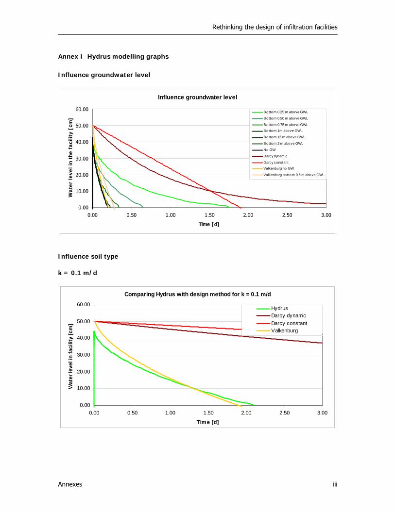
Rethinking the design of infiltration facilities
Annexes iii
Comparing Hydrus with design method for k = 0.1 m/d
0.00
10.00
20.00
30.00
40.00
50.00
60.00
0.00 0.50 1.00 1.50 2.00 2.50 3.00
Time [d]
Wat
er le
vel i
n fa
cilit
y [c
m]
HydrusDarcy dynamic Darcy constant Valkenburg
Annex I Hydrus modelling graphs Influence groundwater level
Influence soil type k = 0.1 m/d
Influence groundwater level
0.00
10.00
20.00
30.00
40.00
50.00
60.00
0.00 0.50 1.00 1.50 2.00 2.50 3.00
Time [d]
Wat
er le
vel i
n th
e fa
cilit
y [c
m]
Bottom 0,25 m above GWL
Bottom 0,50 m above GWL
Bottom 0.75 m above GWL
Bottom 1 m above GWL
Bottom 1,5 m above GWL
Bottom 2 m above GWL
No GW
Darcy dynamic
Darcy constant
Valkenburg no GW
Valkenburg bottom 0.5 m above GWL
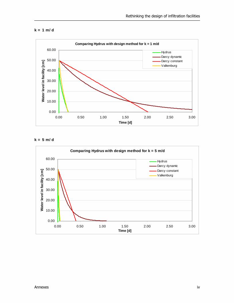
Rethinking the design of infiltration facilities
Annexes iv
Comparing Hydrus with design method for k = 5 m/d
0.00
10.00
20.00
30.00
40.00
50.00
60.00
0.00 0.50 1.00 1.50 2.00 2.50 3.00Time [d]
Wat
er le
vel i
n fa
cilit
y [c
m]
HydrusDarcy dynamic Darcy constant Valkenburg
k = 1 m/d
k = 5 m/d
Comparing Hydrus with design method for k = 1 m/d
0.00
10.00
20.00
30.00
40.00
50.00
60.00
0.00 0.50 1.00 1.50 2.00 2.50 3.00Time [d]
Wat
er le
vel i
n fa
cilit
y [c
m]
HydrusDarcy dynamic Darcy constantValkenburg
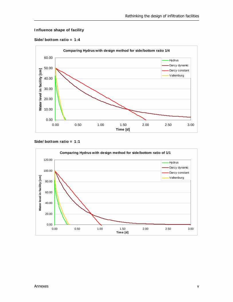
Rethinking the design of infiltration facilities
Annexes v
Influence shape of facility Side/bottom ratio = 1:4
Side/bottom ratio = 1:1
Comparing Hydrus with design method for side/bottom ratio 1/4
0.00
10.00
20.00
30.00
40.00
50.00
60.00
0.00 0.50 1.00 1.50 2.00 2.50 3.00Time [d]
Wat
er le
vel i
n fa
cilit
y [c
m]
Hydrus
Darcy dynamic
Darcy constant
Valkenburg
Comparing Hydrus with design method for side/bottom ratio of 1/1
0.00
20.00
40.00
60.00
80.00
100.00
120.00
0.00 0.50 1.00 1.50 2.00 2.50 3.00Time [d]
Wat
er le
vel i
n fa
cilit
y [c
m]
Hydrus
Darcy dynamic
Darcy constant
Valkenburg
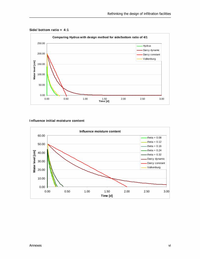
Rethinking the design of infiltration facilities
Annexes vi
Side/bottom ratio = 4:1
Influence initial moisture content
Influence moisture content
0.00
10.00
20.00
30.00
40.00
50.00
60.00
0.00 0.50 1.00 1.50 2.00 2.50 3.00Time [d]
Wat
er le
vel [
cm]
theta = 0.08theta = 0.12theta = 0.16theta = 0.24theta = 0.32Darcy dynamicDarcy constant Valkenburg
Comparing Hydrus with design method for side/bottom ratio of 4/1
0.00
50.00
100.00
150.00
200.00
250.00
0.00 0.50 1.00 1.50 2.00 2.50 3.00Time [d]
Wat
er le
vel [
cm]
Hydrus
Darcy dynamic
Darcy constant
Valkenburg
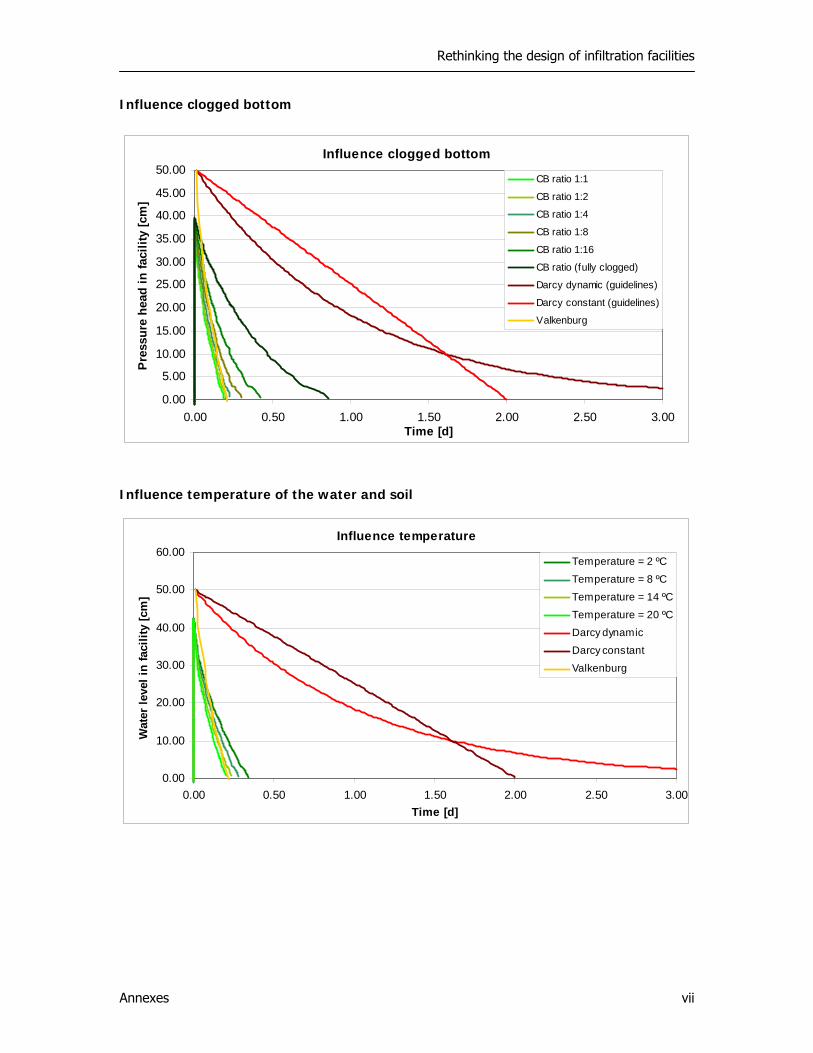
Rethinking the design of infiltration facilities
Annexes vii
Influence clogged bottom
0.00
5.00
10.00
15.00
20.00
25.00
30.00
35.00
40.00
45.00
50.00
0.00 0.50 1.00 1.50 2.00 2.50 3.00Time [d]
Pre
ssur
e he
ad in
faci
lity
[cm
]
CB ratio 1:1
CB ratio 1:2
CB ratio 1:4
CB ratio 1:8
CB ratio 1:16
CB ratio (fully clogged)
Darcy dynamic (guidelines)
Darcy constant (guidelines)
Valkenburg
Influence clogged bottom
Influence temperature of the water and soil
Influence temperature
0.00
10.00
20.00
30.00
40.00
50.00
60.00
0.00 0.50 1.00 1.50 2.00 2.50 3.00Time [d]
Wat
er le
vel i
n fa
cilit
y [c
m]
Temperature = 2 ºC
Temperature = 8 ºC
Temperature = 14 ºC
Temperature = 20 ºC
Darcy dynamic
Darcy constant
Valkenburg

Rethinking the design of infiltration facilities
Annexes viii
Annex II Measuring plan in Ede (in Dutch) Meetplan voor infiltratievoorzieningen in Ede Inleiding De huidige ontwerpbenadering van infiltratievoorzieningen is wetenschappelijk slecht onderbouwd. Het ontwerp wordt gedaan op basis van formules en aannames die eigenlijk niet op infiltratie kunnen worden toegepast. Met veiligheidscoëfficiënten worden de onzekerheden in de ontwerpbenadering afgedekt. Maar juist het stapelen van veiligheidscoëfficiënten kan leiden tot voorzieningen die te groot ontworpen worden. Ook is vanuit beheersoogpunt onbekend zijn zowel de uiteindelijke levensduur als mogelijke onderhoudsmethoden een blinde vlek. Het dichtslibben van infiltratievoorzieningen is een belangrijke onzekerheid op dit gebied. Hoewel er weinig problemen bekend zijn met huidige voorzieningen, is nader onderzoek dus gewenst. De beste methode hiervoor is om aan voorzieningen in de praktijk te meten om het hydraulisch functioneren van de voorzieningen beter in kaart te brengen. De aspecten die van belang zijn voor het ontwerp en het beheer zijn de infiltratie capaciteit en de leeglooptijd van een voorziening. Helaas worden die amper gemeten. De metingen kunnen helpen de ontwerpbenadering te verfijnen én antwoorden geven op beheersvragen op het gebied van levensduur en onderhoud. Doel
- Analyseren welke processen de capaciteit van een infiltratievoorziening tijdens de levensduur beïnvloeden: grondwaterstand, type voorziening, waterstand in de voorziening en dichtslibben.
- Meten van werkelijke leeglooptijd en infiltratiecapaciteit van infiltratievoorzieningen. - Bekijken van de invloed van onderhoud en beheers aspecten van infiltratievoorzieningen:
Hoe kan de infiltratiecapaciteit van een voorziening bekeken en verbeterd worden door onderhoud?
Hypothese De huidige ontwerpbenadering zorgt voor overgedimensioneerde systemen. Dit betekent dat de huidige infiltratiesystemen te groot en dus duurder dan nodig zijn. Het dichtslibben van voorzieningen zorgt ervoor, dat ze anders functioneren dan aangenomen in het ontwerp. Eventueel zou dichtslibben het functioneren van een voorziening kunnen bedreigen. Locaties
- Zakput in het bedrijventerrein in Ede Zuid (Horapark). Dit is de locatie voor de detailstudie
- Krattensysteem in Ede Oost (Buurtscheuterlaan)in het openbaar groen. Ligging in openbaar groen en op zichzelf staand systeem.
Algemeen meetplan Voor het bestuderen van het functioneren van de drie voorzieningen wordt de volgende methode gehanteerd: Met hulp van een tankwagen wordt de voorziening gevuld totdat deze volledig gevuld is. Dan hoeft er niet gewacht te worden op regen. Als de capaciteit van de tankwagen ontoereikend is, wordt de voorziening met de maximale hoeveelheid water gevuld. De voorziening moet wel
Rethinking the design of infiltration facilities
Annexes ix
minimaal voor de helft te gevuld zijn. Een debietmeter is nodig om te weten hoe groot de toevoer naar voorziening is geweest. Vervolgens wordt de infiltratiecapaciteit van de voorziening bekeken en gemonitord. Hiervoor zijn rondom en in de voorzieningen zijn de metingen/meetlocaties in ieder geval nodig:
- De k-waarde omringende grond met infiltroring methode. - Meten van het verloop van de waterstand in voorziening met een diver.
Rekening houden met de weersomstandigheden is belangrijk. Meten kan het beste in een droge periode. Het meten kan het best gepland worden in twee rondes (in twee weken).
1. De eerste ronde worden de verschillende voorzieningen getest. Gedurende enkele dagen worden een zakput, een krattensysteem en evt. doorlatende verharding in Ede gevuld en het infiltratieproces wordt bekeken.
2. De tweede ronde beslaat het detailonderzoek aan het krattensysteem. In de volgende alinea’s wordt verder ingegaan op de specifieke metingen die nodig zijn bij de verschillende voorzieningen. Daarnaast wordt ook een inschatting gemaakt van de benodigde tijd, apparatuur en mankracht. Meetplan zakput De zakputten bevinden in Ede Zuidoost, (nabij de rand van de Veluwe) in het openbaar groen van een bedrijventerrein, het Horapark. Ze zorgen voor de hemelwaterafvoer van het bedrijventerrein. De technische details van de voorziening:
- Maaiveld: + 21.50 m NAP. - Grondsoort: lemig zand, zandig leem (k=0.5-2 m/d) - Grondwaterstand (GHG): + 15 m NAP - Gronddekking: 0.60 m - Omringd door takkenbossenlaag met minimale dikte van 0.7 m - Bodem op + 18.1 m NAP - Betonnen zakput: l x b x h = 1.50 m x 1.50 m x 2.80 m - Overstort op ongeveer 2.40 m (+ 20.5 m NAP), dus nuttige berging = 5.4 m3
Meetronde 1: 1. Opgraven en openen voorziening, 1 uur 2. Visuele inspectie binnenkant, 0.5 uur 3. Installeren diver (zie voor tekening de bijlage), 0.5 uur 4. Volledig vullen, 0,5 uur 5. Meten leegloop, 5 uur (schatting) 6. Meten k waarde, 1 uur
Meetplan krattensysteem Het krattensysteem bevindt zich in Ede Noordoost, nabij de Buurtscheuterlaan in het openbaar groen. De voorziening zorgt voor de hemelwaterafvoer van een deel van de straat en was aangelegd in 2001 om wateroverlast tegen te gaan. De technische details van de voorziening:
- Maaiveld: + 37 m NAP. - Grondsoort: aanname zelfde als bij zakput - Grondwaterstand(GHG): + 17 m NAP., heeft dus geen invloed - Systeem 16 kratten van 810x400x860mm (geeft een berging van 5 m3) - Bovenkant kratten op 36.20 m boven N.A.P., onderkant kratten op 34.48 m boven N.A.P. - Drainzand 10 cm aan onderzijde en 30 cm aan zijkanten aangebracht - Connectie met straat via twee straatkolken, pvc buizen van rond 125 en 160 mm en twee
zandvangen
Rethinking the design of infiltration facilities
Annexes x
Meetronde 1: 1. Opgraven voorziening en buis in voorziening “prikken”, 1 uur 2. Visuele inspectie binnenkant, 0.5 uur 3. Installeren diver (zie voor tekening de bijlage), 0.5 uur 4. Volledig vullen, 0,5 uur 5. Meten leegloop, 5-15 uur (schatting) 6. Meten k waarde, 1 uur 7. Opruimen en afronden, 1 uur
Meetronde 2: 1. Opgraven voorziening en buis in voorziening “prikken”, 0.5 uur 2. Installeren diver en 5 bodemvochtmeters(zie voor tekening de bijlage), 3 uur 3. Volledig vullen, 1 uur 4. Meten leegloop, 5-15 uur (schatting) 5. Opruimen en afronden, 1 uur
Samenvatting benodigde materieel en apparatuur:
- Divers voor het meten van de waterstand (Leon) - Pompwagen voor het vullen van een voorziening (Ede) - Loggers voor het opslaan van metingen (Leon) - Laptop voor het uitlezen van de metingen (Leon) - Communicatie naar omwonenden (Ede)
Algemene planning (onder voorbehoud)
- 10 maart: Uitwerking en planning van meetcampagne
- 18 maart – 20 maart: Meetcampagne deel 1
- 25 maart – 27 maart Meetcampagne deel 2
- Eind maart – begin april: Verwerking resultaten
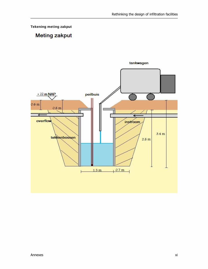
Rethinking the design of infiltration facilities
Annexes xi
Tekening meting zakput
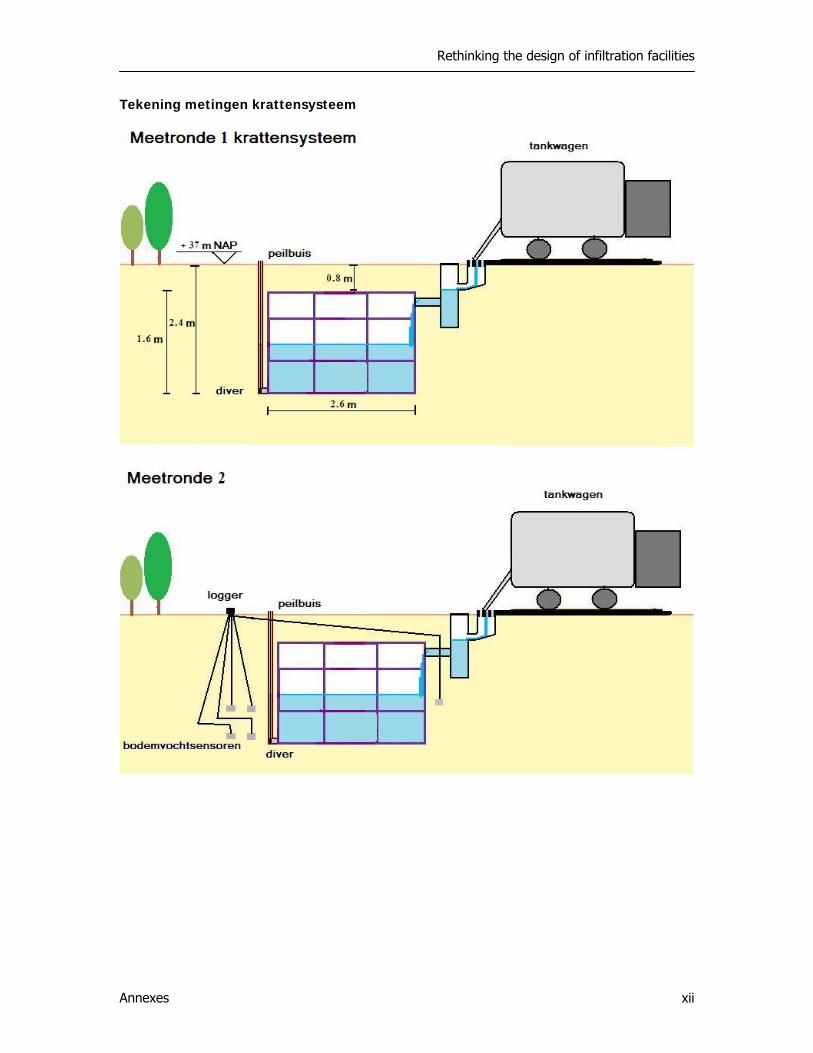
Rethinking the design of infiltration facilities
Annexes xii
Tekening metingen krattensysteem

Rethinking the design of infiltration facilities
Annexes xiii
Annex III Contacted stakeholders
A. The 90 emailed municipalities* for monitoring data *The 19 municipalities marked with an r responded, but had no monitoring information. The 4 municipalities with an m responded and had some monitoring data(not suitable however):
1. Achtkarspelen 2. Alblasserdam 3. Almere 4. Alkmaar (r) 5. Alphen a/d Rijn 6. Amersfoort 7. Amstelveen (r) 8. Amsterdam 9. Anna Palowna 10. Bergen NH (m) 11. Beverwijk (r) 12. Binnenmaas 13. Boarnsterhim 14. Borger-Odoorn (m) 15. Breda 16. Breukelen 17. Brummen (r) 18. Coevorden 19. Dantumadiel 20. De Bilt 21. Den Haag 22. Den Helder 23. Dordrecht 24. Ede (r) 25. Emmen 26. Enkhuizen 27. Gaasterland 28. Haarlemmermeer 29. Haaksbergen (r) 30. Harderwijk (m) 31. Heerenveen (r)
32. Helden 33. Hellendoorn 34. Hendrik Ido
Ambacht 35. Hilversum 36. Hoogeveen 37. Houten 38. Huizen (r) 39. Kollumerland 40. Landsmeer (r) 41. Langedijk 42. Leeuwarderadiel 43. Lemsterland 44. Littenseradiel 45. Loenen 46. Lopik 47. Maarssen 48. Maastricht 49. Midden-Delfland (r) 50. Midden-Drenthe 51. Naarden 52. Nieuwegein 53. Nijkerk 54. Nijmegen (m) 55. Noordenveld 56. Noordwijkerhout 57. Oost-Stellingwerf 58. Opsterland 59. Ouder Amstel 60. Papendrecht 61. Purmerend
62. Raalte 63. Renswoude (r) 64. Renkum (m) 65. Rhenen (r) 66. Rotterdam 67. Schoonhoven 68. Schouwen-
Duiveland (r) 69. ’s Hertogenbosch 70. Sliedrecht 71. Stedebroec (r) 72. Texel 73. Tytsjeksteradiel 74. Utrecht 75. Veenendaal 76. Vianen (r) 77. Vlaardingen 78. Wassenaar 79. Wageningen (r) 80. Westerveld (r) 81. Westland 82. Wieringen 83. Woerden 84. Wunseradiel (r) 85. Woudrichem 86. Wormerland 87. IJsselstein 88. Zaanstad 89. Zijpe (r) 90. Zwolle
B. Interviewed stakeholders Overview of the people interviewed for this research sorted on stakeholder type. Municipalities
• Nijmegen (Antal Zuurman, via telephone) • Renkum (Raymond Leyte) • Ede (various people)
Research institutes
• RIONED (Harry van Luijtelaar) • Deltares (various people)

Rethinking the design of infiltration facilities
Annexes xiii
• TU Delft (various people) Consultants
• Tauw (Floris Boogaard) • DHV (various people)
Infiltration facility’s manufacturers
• Beuker Kunststoffen (Robert Stokkers) • Dyka (Jasper Honingh) • Wavin (Fokko Dijkstra & Louis Wildvank)

Annexes ii