Results of a Precrash Application Based on Laser Scanner ...
11
Results of a Precrash Application Based on Laser Scanner and Short-Range Radars Sylvia Pietzsch, Trung-Dung Vu, Julien Burlet, Olivier Aycard, Thomas Hackbarth, Nils Appenrodt, Jurgen Dickmann, Bernd Radig To cite this version: Sylvia Pietzsch, Trung-Dung Vu, Julien Burlet, Olivier Aycard, Thomas Hackbarth, et al.. Results of a Precrash Application Based on Laser Scanner and Short-Range Radars. IEEE Transactions on Intelligent Transportation Systems, IEEE, 2009, 10 (4), pp.584 - 593. <10.1109/TITS.2009.2032300>. <hal-01023064> HAL Id: hal-01023064 https://hal.archives-ouvertes.fr/hal-01023064 Submitted on 18 Jul 2014 HAL is a multi-disciplinary open access archive for the deposit and dissemination of sci- entific research documents, whether they are pub- lished or not. The documents may come from teaching and research institutions in France or abroad, or from public or private research centers. L’archive ouverte pluridisciplinaire HAL, est destin´ ee au d´ epˆ ot et ` a la diffusion de documents scientifiques de niveau recherche, publi´ es ou non, ´ emanant des ´ etablissements d’enseignement et de recherche fran¸cais ou ´ etrangers, des laboratoires publics ou priv´ es. brought to you by CORE View metadata, citation and similar papers at core.ac.uk provided by Hal - Université Grenoble Alpes
Transcript of Results of a Precrash Application Based on Laser Scanner ...
Results of a Precrash Application Based on Laser
Scanner and Short-Range Radars
Sylvia Pietzsch, Trung-Dung Vu, Julien Burlet, Olivier Aycard, Thomas
Hackbarth, Nils Appenrodt, Jurgen Dickmann, Bernd Radig
To cite this version:
Sylvia Pietzsch, Trung-Dung Vu, Julien Burlet, Olivier Aycard, Thomas Hackbarth, etal.. Results of a Precrash Application Based on Laser Scanner and Short-Range Radars.IEEE Transactions on Intelligent Transportation Systems, IEEE, 2009, 10 (4), pp.584 - 593.<10.1109/TITS.2009.2032300>. <hal-01023064>
HAL Id: hal-01023064
https://hal.archives-ouvertes.fr/hal-01023064
Submitted on 18 Jul 2014
HAL is a multi-disciplinary open accessarchive for the deposit and dissemination of sci-entific research documents, whether they are pub-lished or not. The documents may come fromteaching and research institutions in France orabroad, or from public or private research centers.
L’archive ouverte pluridisciplinaire HAL, estdestinee au depot et a la diffusion de documentsscientifiques de niveau recherche, publies ou non,emanant des etablissements d’enseignement et derecherche francais ou etrangers, des laboratoirespublics ou prives.
brought to you by COREView metadata, citation and similar papers at core.ac.uk
provided by Hal - Université Grenoble Alpes
IEEE TRANSACTIONS ON INTELLIGENT TRANSPORTATION SYSTEMS, VOL. XXX, NO. XXX, XXX 2009 1
Results of a Precrash Application based on
Laser Scanner and Short Range RadarsSylvia Pietzsch, Trung Dung Vu, Julien Burlet, Olivier Aycard, Thomas Hackbarth, Nils Appenrodt,
Jurgen Dickmann, and Bernd Radig
Abstract—In this paper, we present a vehicle safety applicationbased on data gathered by a laser scanner and two short rangeradars that recognizes unavoidable collisions with stationaryobjects before they take place in order to trigger restraintsystems. Two different software modules are compared thatperform the processing of raw data and deliver a descriptionof the vehicle’s environment. A comprehensive experimentalevaluation based on relevant crash and non-crash scenarios ispresented.
Index Terms—Road vehicles, sensor fusion, perception system,collision mitigation.
I. INTRODUCTION
IN recent years, a lot of research has been done to develop
safety applications which help to prevent accidents or
mitigate their consequences [1]. The automatic recognition of
imminent collisions plays an important role in making traffic
safer [2] [3]. The earlier a potential collision is detected, the
more possibilities are available to protect car passengers and
other road users. In this document, we describe a system
to detect frontal collisions. In case a crash is predicted to
happen within the next 200 milliseconds, the system triggers
reversible belt pretensioners which bring the passenger into an
upright position that is safer during the crash and removes the
belt slack in advance. An experimental vehicle was equipped
with sensors and processing hardware to demonstrate the
operational capability of the safety function in real time.
The perception of the environment in front of the vehicle
is based on data from a laser scanner and two short range
radars. The advantages of the laser scanner are its large
field of view and its high angular and range resolution and
accuracy. Labayrade et al. [3], for example, fuse objects from
a laser scanner with objects from a stereovision system for
emergency braking. Other approaches for collision detection
rely on a combination of stereovision and radar, e.g. [4]. Radar
Manuscript received Sept 1, 2008; revised March 2, 2009. This work wassupported in part by the Information Society of the European Union under theContract No. 507075 in the framework of the integrated Project PReVENT.
S. Pietzsch is with the Technische Universitat Munchen, Chair for ImageUnderstanding and Knowledge-based Systems and works cur. for the DaimlerAG, 89081 Ulm, Germany (e-mail: [email protected]).
T. D. Vu, J. Burlet and O. Aycard are with the Laboratoire d’Informatiquede Grenoble and INRIA Rhones Alpes, Grenoble, France (e-mail:[email protected], [email protected], [email protected]).
T. Hackbarth, N. Appenrodt and Dr. J. Dickmann are with the De-partment for Environment Perception, Research Centre of the Daim-ler AG, 89081 Ulm, Germany (e-mail: [email protected],[email protected], [email protected]).
B. Radig is with the Technische Universitat Munchen, Chair for ImageUnderstanding and Knowledge-based Systems, Garching, Germany.
sensors are in common use for driver assistant systems in
cars and complement our system due to immediate velocity
measurements and the use of a complementary emission type.
The methods and software modules presented in this paper
were developed within the Integrated Project PReVENT, a
European research activity to contribute to road safety by
developing preventive safety applications and technologies, co-
funded by the European Commission. The presented work
comprises two different software modules for sensor data
processing that were developed independently by the Daimler
AG (Module 1) and LIG & INRIA Rhones Alpes (Module
2). The perception module 1 and the precrash application are
part of the research done within APALACI (Advanced Pre-
crash And LongitudinAl Collision mitigation), a subproject of
PReVENT with the objective of protecting vehicle occupants.
Perception module 2 was developed within the framework of
PROFUSION2, a subproject that aims at developing concepts
and methods for different sensor data fusion approaches as an
enabler for advanced vehicle safety and assistance functions.
Module 1 utilizes grid-based segmentation of the laser
scanner data and Kalman filter techniques to track objects.
Module 2 is based on simultaneous localization and mapping
techniques (SLAM) together with the detection and tracking
of moving objects. The environment is modeled using an
Occupancy Grid. Detected moving objects are tracked by a
Multiple Hypothesis Tracker (MHT) coupled with an adaptive
Interacting Multiple Models filter (IMM). Our evaluation
compares the performance of both modules on the basis of
the output of a shared precrash decision module by means of
missed and false alarm rates in complex crash and non-crash
maneuvers with stationary objects, respectively.
The remainder of this paper is organized as follows: In
Section II the experimental vehicle together with the sensors
are described. Section III and Section IV deal with the
technical and scientific background of sensor data processing.
They give an overview over the methods that are used within
each of the modules for environmental perception. Section V
explains subsequent processing steps that perform situation
analysis and the decision for or against a collision. Test
results in various driving scenarios are presented in Section VI.
Finally, Section VII summarizes the presented content and
gives suggestions for further work.
II. EXPERIMENTAL VEHICLE AND SENSORS
The experimental vehicle, a Mercedes-Benz E-Class, is
equipped with an Ibeo ”ALASCA” laser scanner mounted
IEEE TRANSACTIONS ON INTELLIGENT TRANSPORTATION SYSTEMS, VOL. XXX, NO. XXX, XXX 2009 2
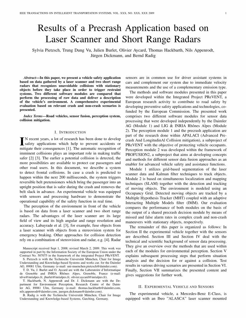
TABLE ITECHNICAL DATA OF THE SENSORS
Property Laser scanner Short range radar
Angle 160◦ 80◦
Angle accuracy +/-0.5◦ +/-5..10◦
Range 0.3-80 m 0.2-30 m
Range accuracy +/-5 cm +/-7.5 cm
Scan frequency 25 Hz 25 Hz
below the number plate and two M/A-COM ”SRS100” 24 GHz
short range radar prototypes mounted in the front bumper
besides the number plate. The laser scanner is hermetically
covered by a box having a black plastic faceplate which is
transparent for the emission wavelength while the radars are
mounted behind the standard plastic bumper. The technical
specifications of the sensors are listed in Table I.
The radar sensors and the laser scanner controller are
connected to a controller unit in the trunk by private CAN
and Ethernet, respectively. This real time unit hosts a 366 MHz
Motorola Power-PC processor which runs the software for sen-
sor data processing, segmentation, object generation, tracking,
sensor data fusion and activation decision.
In case of unavoidable collisions the reversible seatbelt
pretensioners of the front seats are deployed via a private
CAN. An additional PC in the trunk acts as a display server
connected to a monitor in front of the passenger seat to visu-
alize the environment perception and the activation decision.
The architecture of the vehicle is shown in Fig. 1.
Fig. 1. Hardware architecture of the experimental vehicle showing sensors,actuators, computers and interconnects.
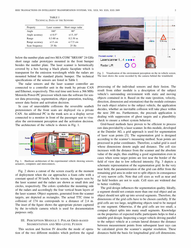
Fig. 2 shows a cutout of the screen exactly at the moment
of deployment when the car approaches a foam cube with a
constant speed of 50 km/h. On the screen, the targets seen by
the laser scanner and the radars are shown as small dots and
circles, respectively. The colors symbolize the mounting side
of the radars and accordingly the four vertical beam layers of
the laser scanner. Object segments, generated from the scanner
targets, are depicted as rectangles. The actual TTC (time to
collision) of 174 ms corresponds to a distance of 2.4 m.
The inset of the figure shows the appropriate picture captured
by the in-vehicle camera which is used for documentation
purposes only.
III. PERCEPTION MODULE 1: POLAR GRID-BASED
SEGMENTATION AND MID-LEVEL FUSION
This section and Section IV describe the mode of opera-
tion of the two different modules which perform the signal
Fig. 2. Visualization of the environment perception on the in-vehicle screen.The inset shows the scene recorded by the camera behind the windshield.
processing of the individual sensors and their fusion. The
result from either module is a description of the subject
vehicle’s surrounding environment with static and moving
objects contained in it. Based on the state (position, velocity,
direction, dimension and orientation) that the module estimates
for each object relative to the subject vehicle, the application
decides, whether an inevitable collision will take place within
the next 200 ms. Furthermore, the precrash application is
dealing with suppression of ghost targets and a plausibility
check to ensure a robust system behavior.
Grid-based methods have proven to be efficient to process
raw data provided by a laser scanner. In this module, developed
at the Daimler AG, a grid approach is used for segmentation
of laser scan points [5]. The segmentation grid is designed
according to the scanner’s measuring method. Scan points are
processed in polar coordinates. Therefore, a radial grid is used
whose dimensions denote angle and distance. The cell size
increases with the distance from the scanner and the absolute
value of the angle, thus enabling a good segmentation even in
cases when some target points are lost near the border of the
field of view due to low reflected intensity. Fig. 3 depicts a
schematic representation of the segmentation grid. In the very
near field, the parameterization of the grid can differ from the
remaining grid area in order not to split objects in consequence
of very narrow cells. Note that cell sizes as well as near and
far field borders are not to scale. Cell sizes are widened due
to better visibility.
The grid design influences the segmentation quality. Ideally,
a segment should not contain more than one real object and an
object should not split up into several segments. Therefore, the
dimensions of the grid cells have to be chosen carefully. If the
grid cells are too large, neighboring objects tend to be merged
to one segment. Otherwise, if the grid cells are too small, a
compact object splits into many small segments. Knowledge
on the properties of expected traffic participants helps to find a
suitable grid design. Inspecting a target vehicle driving parallel
to the subject vehicle at a certain lateral distance the distance
between measurement points from subsequent laser rays can
be calculated given the scanner’s angular resolution. These
distances build the basis for longitudinal grid cell dimensions.

IEEE TRANSACTIONS ON INTELLIGENT TRANSPORTATION SYSTEMS, VOL. XXX, NO. XXX, XXX 2009 3
Fig. 3. Schematic grid design (not to scale) and segmentation procedure.Top: Projection of all scan points onto the grid. Bottom: Marking of grid cellswith no. of points ≥ threshold, connecting of adjacent grid cells and labeling.
Laterally, the cell dimension is set to the physical scanner
resolution at the center of field of view and increases towards
the borders.
In scan segmentation algorithms, there is always a tradeoff
between splitting objects that are located close together and
merging objects that are split into different point clouds due
to missing scan points [6]. Processing single frames without
previous knowledge cannot resolve this ambiguity. Neverthe-
less, the presented method performs moderately well for the
desired application, even with different sized targets.
All scan points of all four vertical layers of the laser scanner
are projected onto the grid. If the number of measurements
within a grid cell exceeds a given threshold the cell is marked
as occupied. Neighboring occupied cells are connected to
form one segment, afterwards. The procedure is illustrated
in Fig. 3. Projecting all scan points onto a one-layered grid
no matter which scan layer they originate from makes the
process efficient in terms of computing time without too
much information loss. Processing each layer separately is also
possible, but in this case, complex logic is needed to combine
the segmentation results from the different layers.
From the obtained segments, features that describe the
properties of an object like dimension or orientation angle
can be extracted. For feature extraction, the minimum angle
point, the point with the shortest distance to the scanner and
the maximum angle point are used to calculate a rectangular
bounding box. The orientation angle denotes the angle between
the longer of the two sides of a segment and the x-axis of the
car coordinate system. As reference point the center of gravity
of all points belonging to one segment is chosen.
The measurements of the laser scanner and the short range
radars are combined using a midlevel fusion approach which
is illustrated in the structure within the large frame in Fig. 4.
Laser scanner data is processed in the way described above.
The radar sensors deliver filtered and pretracked targets. The
sensor interface allows for a back calculation to untracked
targets which is done within the radar preprocessing step.
Coordinate transformation into car coordinate system is per-
formed in this processing stage for each sensor, respectively.
Fig. 4. System architecture. Sensor processing, fusion and tracking arerealized by each module independently. The structure inside the large framedepicts the perception module 1. Situation analysis and the decision step arethe same for both system approaches.
For object tracking, a standard linear Kalman filter is
used [7]. The state vector of an object consists of the x- and
y-position, the x- and y-component of the velocity and the
orientation angle ϕ. Of course, the orientation angle can only
be updated by laser measurements as the radar sensors deliver
point targets only. Beside the estimated state, the dimension
of an object and the information about which sensor has
contributed measurements in the actual time cycle is stored
for each object. Within the Kalman filter a linear kinematic
model is used. Acceleration effects are modeled by adapting
the process noise covariance. The association of measurements
with tracked objects bases on a statistical distance measure.
Association conflicts are resolved using the Global Nearest
Neighbor (GNN) method [8] with a priority scheme based
on object states. The track management distinguishes between
five states of an object (in ascending order of priority): dead,
initiated, tentative, missed and confirmed. There are two kinds
of ambiguity that can occur when associating segments with
objects: an object has more than one segment as candidate for
update and a segment is a candidate for more than one object.
The first ambiguity is resolved by using the GNN method. If
the reference point of a segment lies within the gate of several
objects, the object with higher priority gets the measurement
for update. If states are equal, the dimensions of segment and
objects are compared, and the segment is associated with the
most similar object.
Already tracked objects, that are not confirmed in the
actual time cycle are kept and will only be deleted if no
corresponding object can be assigned during some cycles in
succession. If on the other hand an object can not be associated
with any existing track, a new one is created.
The combination of radar and laser measurements is done
by a measurement vector fusion. Each component c of the
combined measurement vector z = (xz, yz, ϕz)T is calculated
with involvement of the respective variance σ according to (1),
where s is the sensor index and S the maximum number of
IEEE TRANSACTIONS ON INTELLIGENT TRANSPORTATION SYSTEMS, VOL. XXX, NO. XXX, XXX 2009 4
sensors. The fused vector serves as input to the tracking filter.
zc =
∑S
s=0
zc,s
σc,s∑S
s=0
1
σc,s
(1)
The variance of the combined measurements results in
1
σc
=∑S
s=0
1
σc,s
(2)
Attention has to be paid when combining measurements of
different sensors, as reflections can originate from different
parts of an object. For the radar sensors it is unknown, where
the exact reflection center is located on the object. Building
an exact model of the reflectivity is difficult due to immense
variations in object classes and their possible behavior. Similar
to [4], we assume the reflection center to be the object’s nearest
point to the sensor. Before performing the fusion, the position
delivered by radar(s) is corrected with the distance between
the center of gravity (i.e. the reference point) and the nearest
point to scanner of the corresponding segment.
Another aspect when fusing data from different sensors is
the synchronization between them. In our system both the
laser scanner and the radar sensors work with a frequency
of 25 Hz, thus, deliver data every 40ms. Nevertheless, the
exact measuring time cannot be determined. The resulting
synchronization error has influence on the update step within
the Kalman filter, on the one hand, but affects the association
step, on the other hand. Therefore, it must be taken into
account when calculating whether a measurement lies within
the (statistical) gate D of a predicted object.
D2 =(xpred − xmeas)
2
σ2x
+(ypred − ymeas)
2
σ2y
(3)
In (3), xpred and ypred denote the predicted object position
and xmeas, ymeas denote the position of the measurement,
respectively. The total variance does not only include the
process noise and measurement noise, but also a component
representing the synchronization noise:
σ2
x = σ2
x,pred + σ2
x,meas + σ2
x,sync
σ2
y = σ2
y,pred + σ2
y,meas + σ2
y,sync (4)
where σ2sync depends on the cycle time T and on object’s
velocities v (applying 3σ-method):
σ2
x,sync = (1/3 vx · T )2
σ2
y,sync = (1/3 vy · T )2
(5)
In practice, the radar sensors sometimes deliver targets
located outside the gate of an object but inside the object box.
In this case, the information about the object being seen by
this sensor is kept, but the measurement does not contribute
to the fusion.
As with laser segments, ambiguities can occur in associating
radar targets with existing objects. In this case, radar targets
are preferably associated with objects that have laser segments
already associated. If this method fails, the priority scheme as
described for laser segments is applied.
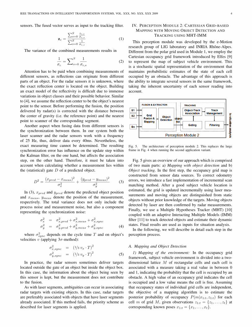
IV. PERCEPTION MODULE 2: CARTESIAN GRID-BASED
MAPPING WITH MOVING OBJECT DETECTION AND
TRACKING USING MHT-IMM
This perception module was developed by the e-Motion
research group of LIG laboratory and INRIA Rhone-Alpes.
Different from the polar grid used in Module 1, we employ the
Cartesian occupancy grid framework introduced by Elfes [9]
to represent the map of subject vehicle environment. This
is a stochastic spatial representation of the environment that
maintains probabilistic estimates of the state of each cell
occupied by an obstacle. The advantage of this approach is
the ability to integrate several sensors in the same framework,
taking the inherent uncertainty of each sensor reading into
account.
Fig. 5. The architecture of perception module 2. This replaces the largeframe in Fig. 4 when running the second application variant.
Fig. 5 gives an overview of our approach which is comprised
of two main parts: a) Mapping with object detection and b)
Object tracking. In the first step, the occupancy grid map is
constructed from sensor data sources. To correct odometry
errors, we introduce a fast implementation of incremental scan
matching method. After a good subject vehicle location is
estimated, the grid is updated incrementally using laser mea-
surements and moving objects are distinguished from static
objects without prior knowledge of the targets. Moving objects
detected by laser are then confirmed by radar measurements.
Finally, we use a Multiple Hypotheses Tracker (MHT) [10]
coupled with an adaptive Interacting Multiple Models (IMM)
filter [11] to track detected objects and estimate their dynamic
states. Final results are used as inputs for situation analysis.
In the following, we will describe in detail each step in the
perception process.
A. Mapping and Object Detection
1) Mapping of the environment: In the occupancy grid
framework, subject vehicle environment is divided into a two-
dimensional lattice M of rectangular cells and each cell is
associated with a measure taking a real value in between 0
and 1, indicating the probability that the cell is occupied by an
obstacle. A high value of an occupancy grid indicates the cell
is occupied and a low value means the cell is free. Assuming
that occupancy states of individual grid cells are independent,
the objective of a mapping algorithm is to estimate the
posterior probability of occupancy P (m|x1:t, z1:t) for each
cell m of grid M , given observations z1:t = {z1, . . . , zt} at
corresponding known poses x1:t = {x1, . . . , xt}.

IEEE TRANSACTIONS ON INTELLIGENT TRANSPORTATION SYSTEMS, VOL. XXX, NO. XXX, XXX 2009 5
Here we apply the Bayesian update scheme similar to that
proposed in [12] which provides an elegant recursive formula
to update the posterior under log-odds form:
log O(m |x1:t, z1:t) = log O(m |x1:t−1, z1:t−1) +
+ log O(m | zt, xt) − log O(m) (6)
where O(a) = odds(a) = P (a) / (1 − P (a))
In (6), P (m) is the prior occupancy probability of the map
which is initially set to 0.5 representing an unknown state, this
makes this component disappeared. The remaining probability
P (m|xt, zt) is called the inverse sensor model. It specifies the
probability that a grid cell m is occupied based on a single
sensor measurement zt at location xt. In our implementation,
it is decided by the measurement of the nearest beam to
the center mass of the cell. Note that the desired probability
of occupancy P (m|x1:t, z1:t) can be easily recovered from
the log odds representation. Moreover, since the updating
algorithm is recursive, it allows for incremental map updating
when new sensor data arrives. Fig. 6 shows examples of an
occupancy grid map where the gray color level of grid cells
indicates the probability of the corresponding space being
occupied: gray=unknown, white=free, black=occupied.
2) Vehicle Localization: In order to build a consistent map
of the environment, a good subject vehicle localization is
required. Because of the inherent error, using only odometry
often results in an unsatisfying map. When features can not
be defined and extracted, direct scan matching techniques
like ICP and its variants [13] are popular ways to correct
vehicle location. The most evident flaw of these ICP-style
scan matching methods is that the measurement uncertainty
is not taken into account. Especially, sparse data and dynamic
entities in outdoor environment cause problems of correspon-
dence finding in ICP-style methods which affect the accuracy
of matching results.
An alternative approach that can overcome these limitations
consists of setting up the matching problem as a maximum
likelihood problem. In this approach, given an underlying
vehicle dynamics constraint, the current scan’s position is
corrected by comparing with the local grid map constructed
from all observations in the past instead of only with one
previous scan. In this way we can reduce the ambiguity and
weak constraint especially in outdoor environment and when
the subject vehicle moves at high speeds.
Mathematically, we calculate a sequence of poses x1, x2, . . .and sequentially updated maps M1, M2, . . . by maximizing the
marginal likelihood of the t-th pose and map relative to the
(t − 1)-th pose and map:
xt = argmaxxt{P (zt|xt, Mt−1).P (xt|xt−1, ut)} (7)
In (7), the term P (zt|xt, Mt−1) is the measurement model
which is the probability of the most recent measurement zt
given the pose xt and the map Mt−1 constructed so far from
observations z1:t−1 at corresponding poses x1:t−1 that were
already estimated in the past.
The term P (xt|xt−1, ut) represents the motion model which
is the probability that the subject vehicle is at location xt given
that the subject vehicle was previously at position xt−1 and
executed an action ut. The resulting pose xt is then used to
generate a new map Mt according to (8):
Mt = Mt−1 ∪ {xt, zt} (8)
For the motion model, we adopt the probabilistic velocity
motion model similar to that of [12]. The vehicle motion
ut is comprised of two components, the translational velocity
vt and the yaw rate ωt. The distribution is obtained from
the kinematic equations and modeling noise of rotational
and translational components. For the measurement model
P (zt|xt, Mt−1), to avoid ray casting, we propose a method
that only considers end-points of the beams. Because it is
likely that a beam hits an obstacle at its end-point, we only
focus on occupied cells in the grid map. For those cells, a sum
proportional to the occupancy value will be voted. The final
voted score represents the probability of a scan measurement
zt given the vehicle pose xt and the map Mt−1 constructed
so far (Fig. 6). Readers could refer to [14] for more details.
Fig. 6. The subject vehicle location is obtained by trading off the consistencyof laser measurement with the grid map and the vehicle ego motion.
3) Local Mapping: Because we do not need to build a
global map nor deal with loop closing problem, only one
online map is maintained at each point in time representing
the local environment surrounding the subject vehicle. The size
of the local map is chosen so that it should not contain loops
and the resolution is maintained at a reasonable level. Every
time the subject vehicle arrives near the map boundary, a new
grid map is initialized. The pose of the new map is computed
according to the subject vehicle’s global pose and cells inside
the intersection area are copied from the old map.
4) Moving Object Detection: After obtaining a good lo-
calization of the subject vehicle, a consistent local map is
constructed. From the constructed grid, moving objects can
be detected when new measurements arrive. The principal
idea is based on the inconsistencies between observed free
space and occupied space in the local grid map. If an object
is detected in a location previously seen as free space, then
it is a moving object. If an object is observed on a location
previously occupied then it probably is static.
Another important clue which can help to decide whether
an object is dynamic or not is the evidence about moving
objects detected in the past. For example, if there are many
moving objects passing through an area then any object that
appears in that area should be recognized as a potential moving
object. For this reason, apart from the local static map M as
constructed in the previous section, a local dynamic grid map
D is created to store information about previously detected

IEEE TRANSACTIONS ON INTELLIGENT TRANSPORTATION SYSTEMS, VOL. XXX, NO. XXX, XXX 2009 6
moving objects. The size and resolution of the dynamic map
are the same as those of the static map. Each dynamic grid
cell stores a value indicating the number of observations that
a moving object has been observed at that cell.
From these remarks, our moving object detection process is
carried out in two steps as follows. The first step is to detect
measurements that might belong to dynamic objects. Here for
simplicity, we will temporarily omit the time index. Given a
new laser scan z, the corrected subject vehicle location and
the local static map M and the dynamic map D containing
information about previously detected moving objects, state of
a single measurement zk is classified into one of three types
following: static if Mhit is occupied, dynamic if Mhit is free or
Dhit > α, undecided otherwise; where Mhit and Dhit are the
corresponding cells of the static and dynamic map respectively
at the end-point of the beam zk, α is a pre-defined threshold.
The second step is performed after measurements belonging
to dynamic objects are determined. Moving objects are iden-
tified by clustering end-points of these beams into separate
groups, each group represents a single object. Two points are
considered as belonging to the same object if the distance
between them is less than 0.2 m.
Fig. 7 illustrates the moving object detection process. The
leftmost image depicts the situation where the subject vehicle
is moving along a street seeing a car moving ahead and a
motorbike moving in the opposite direction. The middle image
shows the local static map and the subject vehicle location and
the current laser scan is displayed in black (resp. red) color.
Measurements which fall into free region in the static map
are detected as dynamic and are displayed in the rightmost
image. After the clustering step, two moving objects (in boxes)
are identified and correctly correspond to the car and the
motorbike.
Fig. 7. Example for moving object detection. The big rectangle representsthe subject vehicle.
5) Fusion with radar: After moving objects are identified
from laser data, we confirm the detection results by fusing
with radar data. Since data returned from radar sensors are
pre-filtered as lists of potential targets, each target in the lists is
provided with information about the location and the estimated
Doppler velocity, the data fusion is performed at object-level.
For each object detected by laser as described in the
previous section, a rectangular bounding box is calculated and
the radar measurements which lie within the box region are
then assigned to the corresponding object. The velocity of the
detected moving object is estimated as the average of these
corresponding radar measurements.
Fig. 8 shows an example of how the fusion process takes
place. Moving objects detected by laser data are displayed as
dots within bounding boxes. The targets detected by two radar
sensors are represented as circles along with corresponding
velocities. We can see in the radar field of view, two objects
detected by laser data are also seen by two radars so that they
are confirmed. Radar measurements that do not correspond to
any dynamic object or fall into other region of the grid are
not considered.
Fig. 8. Moving objects detected from laser data are confirmed by radar data.
B. Object Tracking
In the second level, moving objects detected in the vehicle
environment are tracked. Since some objects may be occluded
or some are false alarms or not detected, object tracking helps
to identify occluded objects, recognize false alarms and reduce
misdetections.
In general, the multiple object tracking problem is complex:
it includes the definition of filtering methods, association
methods and maintenance of the list of objects currently
present in the environment. Regarding filtering techniques,
Kalman filters [7] or particle filters [15] are generally used.
These filters require the definition of a specific dynamic model
of tracked objects. However, defining a suitable motion model
is a real difficulty. To deal with this problem, Interacting
Multiple Models [16] have been successfully applied in several
applications. The IMM approach overcomes the difficulty
due to motion uncertainty by using more than one motion
model. The principle is to assume a set of models as possible
candidates for the true displacement model of the object at
one time. To do so, a bank of elemental filters is run at each
time, each corresponding to a specific motion model, and the
final state estimation is obtained by merging the results of all
elemental filters according to the distribution probability over
the set of motion models.
In the previous work [11], we have developed a fast method
to adapt on-line IMM according to trajectories of detected
objects and so we obtain a suitable and robust tracker. To deal
with the data association and track maintenance problem, we
extend our approach to multiple object tracking using Multiple
Hypotheses Tracker [10]. The basic principle of MHT is to
generate and update a set of association hypotheses during
processing. A hypothesis corresponds to a specific probable
assignment of observations with tracks. By maintaining and
updating several hypotheses, association decisions are made
and ambiguous cases are solved in further steps.
As shown in Fig. 5, our multiple object tracking method
is composed of four different steps. In the first step (gat-
ing), based on predictions from previous computed tracks,
we compute the set of new detected objects which can be
IEEE TRANSACTIONS ON INTELLIGENT TRANSPORTATION SYSTEMS, VOL. XXX, NO. XXX, XXX 2009 7
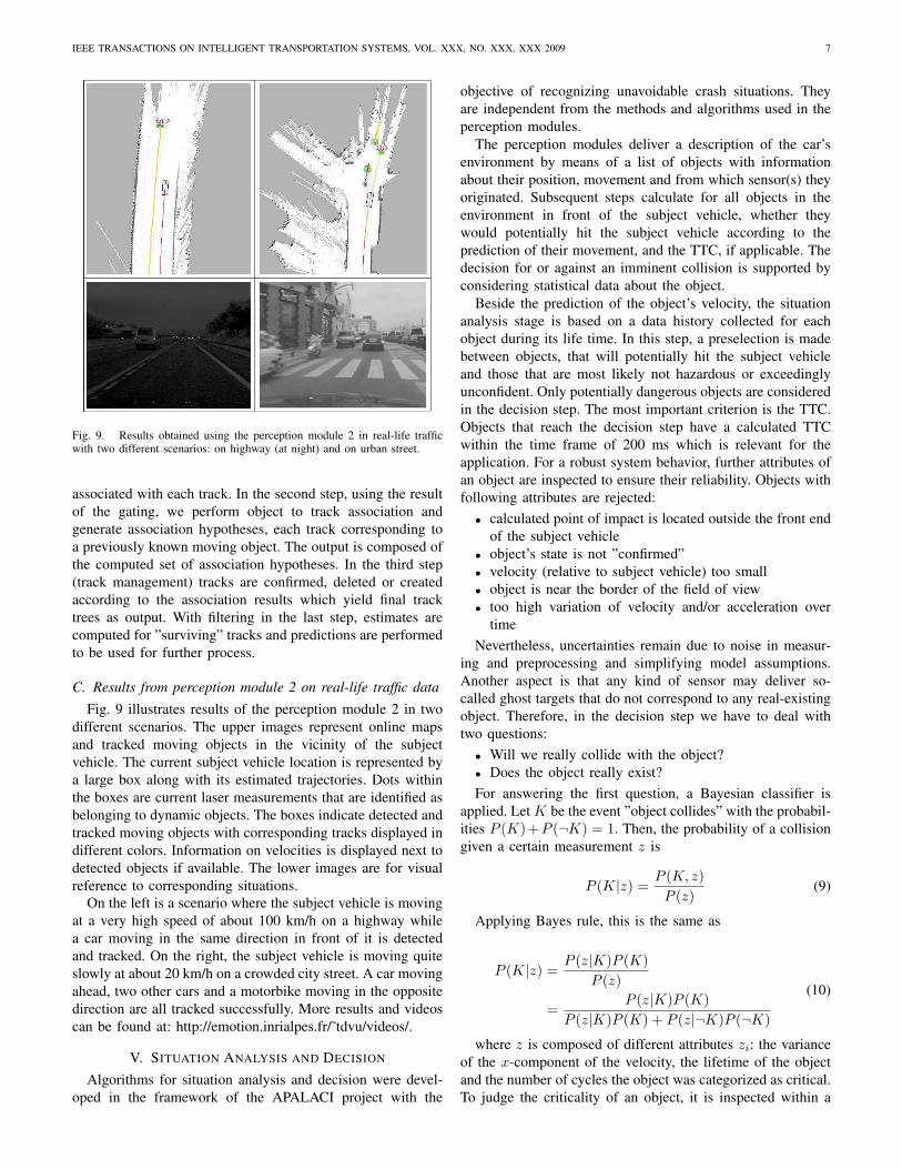
Fig. 9. Results obtained using the perception module 2 in real-life trafficwith two different scenarios: on highway (at night) and on urban street.
associated with each track. In the second step, using the result
of the gating, we perform object to track association and
generate association hypotheses, each track corresponding to
a previously known moving object. The output is composed of
the computed set of association hypotheses. In the third step
(track management) tracks are confirmed, deleted or created
according to the association results which yield final track
trees as output. With filtering in the last step, estimates are
computed for ”surviving” tracks and predictions are performed
to be used for further process.
C. Results from perception module 2 on real-life traffic data
Fig. 9 illustrates results of the perception module 2 in two
different scenarios. The upper images represent online maps
and tracked moving objects in the vicinity of the subject
vehicle. The current subject vehicle location is represented by
a large box along with its estimated trajectories. Dots within
the boxes are current laser measurements that are identified as
belonging to dynamic objects. The boxes indicate detected and
tracked moving objects with corresponding tracks displayed in
different colors. Information on velocities is displayed next to
detected objects if available. The lower images are for visual
reference to corresponding situations.
On the left is a scenario where the subject vehicle is moving
at a very high speed of about 100 km/h on a highway while
a car moving in the same direction in front of it is detected
and tracked. On the right, the subject vehicle is moving quite
slowly at about 20 km/h on a crowded city street. A car moving
ahead, two other cars and a motorbike moving in the opposite
direction are all tracked successfully. More results and videos
can be found at: http://emotion.inrialpes.fr/˜tdvu/videos/.
V. SITUATION ANALYSIS AND DECISION
Algorithms for situation analysis and decision were devel-
oped in the framework of the APALACI project with the
objective of recognizing unavoidable crash situations. They
are independent from the methods and algorithms used in the
perception modules.
The perception modules deliver a description of the car’s
environment by means of a list of objects with information
about their position, movement and from which sensor(s) they
originated. Subsequent steps calculate for all objects in the
environment in front of the subject vehicle, whether they
would potentially hit the subject vehicle according to the
prediction of their movement, and the TTC, if applicable. The
decision for or against an imminent collision is supported by
considering statistical data about the object.
Beside the prediction of the object’s velocity, the situation
analysis stage is based on a data history collected for each
object during its life time. In this step, a preselection is made
between objects, that will potentially hit the subject vehicle
and those that are most likely not hazardous or exceedingly
unconfident. Only potentially dangerous objects are considered
in the decision step. The most important criterion is the TTC.
Objects that reach the decision step have a calculated TTC
within the time frame of 200 ms which is relevant for the
application. For a robust system behavior, further attributes of
an object are inspected to ensure their reliability. Objects with
following attributes are rejected:
• calculated point of impact is located outside the front end
of the subject vehicle
• object’s state is not ”confirmed”
• velocity (relative to subject vehicle) too small
• object is near the border of the field of view
• too high variation of velocity and/or acceleration over
time
Nevertheless, uncertainties remain due to noise in measur-
ing and preprocessing and simplifying model assumptions.
Another aspect is that any kind of sensor may deliver so-
called ghost targets that do not correspond to any real-existing
object. Therefore, in the decision step we have to deal with
two questions:
• Will we really collide with the object?
• Does the object really exist?
For answering the first question, a Bayesian classifier is
applied. Let K be the event ”object collides” with the probabil-
ities P (K)+P (¬K) = 1. Then, the probability of a collision
given a certain measurement z is
P (K|z) =P (K, z)
P (z)(9)
Applying Bayes rule, this is the same as
P (K|z) =P (z|K)P (K)
P (z)
=P (z|K)P (K)
P (z|K)P (K) + P (z|¬K)P (¬K)
(10)
where z is composed of different attributes zi: the variance
of the x-component of the velocity, the lifetime of the object
and the number of cycles the object was categorized as critical.
To judge the criticality of an object, it is inspected within a
IEEE TRANSACTIONS ON INTELLIGENT TRANSPORTATION SYSTEMS, VOL. XXX, NO. XXX, XXX 2009 8
determined time period that is longer than the TTC. Assum-
ing independent attributes zi and, furthermore, K and ¬Kequiprobable, the probability of a collision can be calculated
using (11).
P (K|z) =
∏P (zj |K)∏
P (zj |K) +∏
P (zj |¬K)(11)
The conditional probabilities P (zj |K) and P (zj |¬K) are
determined beforehand in an offline procedure by inspecting
numerous examples with different situations. Finally, an object
is considered as crashing object if P (K|z) exceeds a prede-
fined threshold.
Beside the probability of a collision, the probability of
existence has to be considered in order to prevent false alerts
that may arise from ghost targets delivered by the sensors or
failures in associating measurements with objects. We use a
method based on evidence theory introduced by Dempster and
Shafer [17] [18].
For a classification of existing and non-existing objects we
define the hypothesis space as Θ = {E,¬E} where E stands
for ”object exists” and ¬E stands for ”object does not exist”.
In evidence theory the power set 2Θ = {∅, E,¬E,E∪¬E} is
considered. Sensor-specific mass functions assign probability
masses to the elements in the power set. For the laser scanner,
the mass functions are implemented as:
ml(E ∪ ¬E) = cl
ml(E) =
∑N
i=02N−i · hl[i]∑N
i=02N−i
· (1 − ml(E ∪ ¬E))
ml(¬E) = 1 − (ml(E) + ml(E ∪ ¬E))
(12)
By definition, ml(∅) = 0. The constant term cl denotes
a mass probability for uncertainty. The mass function for
the hypothesis ”object exists” considers the weighted ratio of
the number of detections to the lifetime of an object within
a given time frame N . In this connection, hl[i] contains
the information about the object being detected by the laser
scanner at time i. Younger data is exponential higher weighted
than older data. The remaining mass for the hypothesis ”object
does not exist” is derived from the condition∑
X⊆Θm(X) = 1 (13)
Mass functions for radar sensors are implemented in an
analogous way. The fusion of masses from the different
sensors is performed in two steps. First, the masses from the
two radar sensors are combined. Second, the resulting radar
masses are combined with the masses calculated for the laser
scanner. For fusion, Dempster’s combination rule is used [18].
The final step of the decision module combines the prob-
ability of collision that is provided by the Bayes classifier
with the probability of existence. For the Bayes classifier we
define the hypothesis space Θ = {C,¬C} with the hypothesis
C for a colliding object and ¬C for a non-colliding object.
The probability masses mb(C) and mb(¬C) are directly taken
from the conditional probabilities for K (see (11)).
mb(C) = P (K|z)
mb(¬C) = P (¬K|z) = 1 − mb(C)
mb(C ∪ ¬C) = 0
(14)
In this case, the uncertainty C ∪ ¬C is equal to zero,
because Bayesian probabilities do not provide a measure
for uncertainty. For the interesting case ”object exists and
collides” the combined probability mass results in
mf (E ∩ C) = mb(C) · (mc(E) + mc(E ∪ ¬E)) (15)
If mf exceeds a predefined threshold, actuators are trig-
gered.
In general, laser measurements are able to describe the
position and shape of real existing objects very accurately.
Radar sensors help to suppress ghost targets or targets based
on objects that are irrelevant for precrash applications like
plants or steam coming out of street drains. All in all, the
presented precrash system based on a laser scanner fused with
short range radars reliably detects different kinds of collisions
with stationary objects in front of the car, as our evaluation in
Section VI shows.
VI. EXPERIMENTAL RESULTS
The application has been validated in complex crash and
non-crash scenarios. To conduct the experiments, we built up
a comprehensive database that consists of short sequences of
measurements recorded during predefined driving maneuvers.
These maneuvers comprise factual and near missed collisions
with stationary objects at different velocities, in curves, with
deceleration, sudden lane changes and lane changes of a
leading target vehicle obstructing the sight to the obstacle.
In the maneuvers, foam cubes and cylinders served as crash
objects. To measure the quality, we counted the false alarms
that occurred in non-crash scenarios and the missed alarms in
case a collision was not detected by the application. Table II
compares the results for the non-crash scenarios for the two
different modules and Table III lists the results for the crash
scenarios.
As a general result it can be stated that a reliable collision
detection is achieved with both perception modules. Whereas
Module 1 enables a lower false alarm rate, the crash detection
rate of Module 2 is very high (98.1%). The three false alarms
in the scenario where we pass the cylinder in a curve occurred
in cases of getting extremely close to the obstacle. In contrast,
no false alarms occurred at all when the subject vehicle
suddenly changes the lane to avoid a collision with an obstacle
standing on the road. Emergency brake maneuvers challenge
the tracking system because of the divergent motion scheme.
In our evaluation, only 1 out of 19 test drives resulted in a
false alarm for each module.
In motion estimation, there is always a tradeoff between
stabilization of the current state and the adaptation to dynamic
situations. It becomes apparent when looking at the scenarios
where the system fails. In case of cornering, for example,
the direction of the obstacle’s relative movement continuously
changes. From the results in curve scenarios, it can be seen,
that the two modules handle such situation in a different
way. Module 2 produces more false alarms, whereas Module
1 risks more missed alarms. Looking at Table III, missed
alarms provoked by Module 1 are overrepresented in high
speed scenarios. An object with a high relative velocity is
IEEE TRANSACTIONS ON INTELLIGENT TRANSPORTATION SYSTEMS, VOL. XXX, NO. XXX, XXX 2009 9
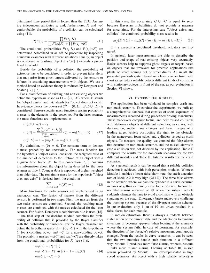
TABLE IIRESULTS FOR COMPLEX NON-CRASH SCENARIOS
Scenario Ego velocity [km/h] Number of tests False alarms/False alarm rate
Module 1 Module 2
Near-missed passing of cylinder 40, 60 9 0 / 0% 0 / 0%
Near-missed passing of cube 40, 60 6 0 / 0% 0 / 0%
Near-missed passing of cylinder after curve (45◦) 40, 60 29 0 / 0% 3 / 10.3%
Emergency brake, distance to cylinder after brake not greater than 1.5 m 40, 60 (at start) 19 1 / 5.3% 1 / 5.3 %
Lane change maneuver to avoid a collision with a cube 30, 40, 50, 60, 70 22 0 / 0% 0 / 0%
Gate passing 30, 50 6 0 / 0% 0 / 0%
Gate passing after curve (45◦) 30, 50 4 0 / 0% 0 / 0%
Total 95 1 / 1.1% 4 / 4.2%
TABLE IIIRESULTS FOR COMPLEX CRASH SCENARIOS
Scenario Ego velocity [km/h] Number of tests Missed alarms/Missed alarm rate
Module 1 Module 2
Collision with cylinder, varying points of impact 20, 40 24 0 / 0% 0 / 0%
Collision with (paper) cylinder at high speed, varying points of impact 60, 120 8 2 / 25.0% 0 / 0%
Collision with cube, point of impact has high offset 40 7 0 / 0% 1 / 14.3%
Collision with cylinder after curve (30◦, 45◦) 30, 40, 60 20 2 / 10.0% 0 / 0%
Collision with cylinder or cube after emergency brake 20, 40 (at crash time) 7 0 / 0% 0 / 0%
Collision with (paper) cylinder after emergency brake at high speed 60, 80 (at crash time) 9 2 / 22.2% 0 / 0%
Collision with cylinder after lane change maneuver 40, 50 23 1 / 4.3% 1 / 4.3%
Collision with cylinder after leading car lane change 40, 50 4 0 / 0% 0 / 0%
Total 102 7 / 6.9% 2 / 1.9%
registered infrequently during the time period available for
creating a data history for this object as described in Section V.
In this case, the decision is supported by less data. Depending
on the influence of new measurements on the current state,
the grid map approach may be advantageous over a single
frame processing realized in Module 1, in this special case.
In general, it should be highlighted that a lot of the test
maneuvers have been performed at the vehicle dynamics limit.
In a third experiment we tested the application in normal
traffic on highways, rural roads and in urban areas. To achieve
representative results we performed the test drives during day
time to cover different traffic situations like rush hour, traffic
jam and stop-and-go. Furthermore, the test drives were partly
conducted under adverse weather conditions like rain, fog,
wet roads and traffic spray. All in all, we covered a distance
of 1600 km, running the application in real time. This test
was performed within the framework of the APALACI project
using the perception module 1 only. There were no wrongly
detected collisions in any of these environments.
VII. CONCLUSION AND OUTLOOK
In this paper we compared two approaches that perform
the data processing and object generation fusing laser scanner
and short range radar sensors. The obtained description of the
vehicle’s environment in terms of static and moving objects
serves as a basis for safety systems that trigger restraint
systems in case an unavoidable collision will take place.
Comprehensive tests show, that a good detection perfor-
mance for frontal collisions is achieved with both approaches.
Comparing the results of both approaches, the sums of false
and missed alarms balance each other. The application was
running stably in a hard real-time environment and has been
extensively tested in real traffic scenarios and with artificial
crash and near crash maneuvers carried out on test tracks. The
function has been successfully demonstrated in a public event
during the 2007 PReVENT IP Exhibition in Versailles and at
the IEEE Intelligent Vehicles Symposium, 2008, in Eindhoven.
Future works will extend the perception modules in order
to improve the detection of collisions with moving objects
and with the major goal to shift the activation decision to
a time earlier than 200ms. This includes the refinement of
motion models and object models to give a more meaningful
representation of detected objects with specific shapes and
behavior.
REFERENCES
[1] A. Vahidi and A. Eskandarian, Research Advances in Intelligent Colli-
sion Avoidance and Adaptive Cruise Control, IEEE Trans. Intell. Transp.Syst., vol. 4, nr. 3, 2003, pp.143-153.
[2] J. Hillenbrand, A. M. Spieker and K. Kroschel, A Multilevel Collision
Mitigation Approach–Its Situation Assessment, Decision Making, and
Performance Tradeoffs, IEEE Trans. Intell. Transp., vol. 7, nr. 4, 2006,pp. 528-540
[3] R. Labayrade, C. Royere and D. Aubert, A Collision Mitigation System
using Laser Scanner and Stereovision Fusion and its Assessment, Proc.IEEE Intell. Veh. Symp., 2005, pp. 441-446
[4] S. Wu, S. Decker, P. Chang, T. Camus and J. Eledath, Collision Sensing
by Stereo Vision and Radar Sensor Fusion, Proc. IEEE Intell. Veh.Symp., 2008, pp. 404-409
[5] M. Skutek, D.T. Linzmeir, N. Appenrodt and G. Wanielik, A Precrash
System based on Sensor Data fusion of Laser Scanner and Short Range
Radars, Proc. IEEE Int. Conf. on Inform. Fusion, 2005, pp. 1287-1295.
IEEE TRANSACTIONS ON INTELLIGENT TRANSPORTATION SYSTEMS, VOL. XXX, NO. XXX, XXX 2009 10
[6] D. Streller and K. Dietmayer, Object Tracking and Classification Using
a Multiple Hypothesis Approach, Proc. IEEE Intell. Veh. Symp., 2004,pp. 808-812
[7] R.E. Kalman, A New Approach to Linear Filtering and Prediction
Problems, in Transactions of the ASME-Journal of Basic Engineering,1960, vol. 82, pp. 35-45.
[8] Y. Bar-Shalom and T.E. Fortmann, Tracking and Data Association,Orlando, Academic Press, 1988.
[9] A. Elfes, Occupancy grids: a probabilistic framework for robot percep-
tion and navigation, Ph.D. dissertation, Carnegie Mellon Univ., 1989.[10] S.S. Blackman, Multiple hypothesis tracking for multiple target tracking,
IEEE Aerosp. Electron. Syst. Mag., 19 (1), 2004, pp. 5-18.[11] J. Burlet, O. Aycard, A. Spalanzani and C. Laugier, Adaptive Interactive
Multiple Models applied on pedestrian tracking in car parks, in Proc.IEEE Int. Conf. on Intelligent Robots and Systems, 2006, pp. 525-530.
[12] S. Thrun, W. Burgard, and D. Fox, Probabilistic Robotics (Intelligent
Robotics and Autonomous Agents), The MIT Press, September 2005.[13] S. Rusinkiewicz and M. Levoy. Efficient variants of the icp algorithm,
2001.[14] T.D. Vu, O. Aycard, and N. Appenrodt, Online localization and map-
ping with moving object tracking, in Proc. IEEE Intelligent VehiclesSymposium, Istanbul, 2007, pp. 190-195.
[15] S. Arulampalam, S. Maskell, N. Gordon, T. Clapp, A tutorial on
particle filter for online nonlinear/non-gaussian bayesian tracking, IEEETransactions on Signal Processing, 50 (2).
[16] E. Mazor, A. Averbuch, Y. Bar-Shalom, J. Dayan, Interacting multiple
model methods in target tracking: a survey, IEEE Transactions onAerospace and Electronic Systems, 34 (1), 1998, pp. 103123.
[17] G. Shafer, A mathematical theory of evidence, Princeton UniversityPress, 1976.
[18] A. Dempster, A Generalization of Bayesian Inference, in Journal of theRoyal Statistical Society, vol. 30, 1968, pp. 205-247.
Sylvia Pietzsch received her diploma in ComputerScience from the Technische Universitat Munchen,Germany, in 2007. Currently, she is with the Chairfor Image Understanding and Knowledge-based Sys-tems of the Technische Universitat Munchen asa doctoral candidate. She pursues her studies atthe Daimler AG, Department for Environment Per-ception. Her research interests include sensor dataprocessing and fusion for driver assistance systems.
Trung Dung Vu is a PhD candidate at INRIA Rhne-Alpes Grenoble since 2006. He received his BScfrom the Faculty of Technology, Vietnam NationalUniversity in 2001 and his MSc from the Insti-tute National Polytechnique de Grenoble (INPG) in2005. His research interests include range sensorprocessing, computer vision and machine learning.
Julien Burlet obtained his PhD in Mathematicsand Computer Science from the Institute NationalPolytechnique de Grenoble (INPG), France in 2007.His knowledge and interest in machine learning andautonomous systems is demonstrated by more thanten publications in this field addressing localisation,multiple object tracking and classification. In 2008,Julien Burlet joined TRW-Conekt, Solihull, UK as aresearch and development engineer. Since then, hepursued his research on object detection, trackingand classification with radars and cameras while
focusing on Automotive and Ministry of Defence applications.
Olivier Aycard received his PhD in Computer Sci-ence from the University of Nancy in 1998. In 1999,he was visiting researcher at Nasa Ames ResearchCenter in Moffett Field, CA. Since 2000, OlivierAycard is an Associate Professor at University ofGrenoble. His researches focus on Bayesian tech-niques for perception with an emphasis on multi-objects tracking using multi-sensor approaches. Hehas more than 40 publications in this field. Hewas also involved in several national and europeanprojects in collaboration with european car manufac-
turers (Daimler, VW, Volvo, Peugeot). In addition, he is in charge of lecturesin Artificial Intelligence and Autonomous Robotics at University of Grenoble.
Thomas Hackbarth was born on August 28, 1958in Stade, Germany. He received the Diploma andPhD degrees in electrical engineering from theTechnical University of Braunschweig, Germany in1986 and 1991, respectively. In 1991, he joinedthe Research and Technology department of theDaimler AG in Ulm, Germany. After several yearsof semiconductor technology research, he changedhis field of activity to the development of active andpassive safety systems.
Nils Appenrodt received the Diploma degree (Dipl.-Ing.) in electrical engineering from the UniversitatDuisburg, Germany, in 1996. He was research as-sistant in the field of imaging radar systems at theUniversitat Duisburg working in close cooperationwith DaimlerChrysler research institute, Ulm. Since2000 he has been with Daimler AG, Group Research,Ulm, mainly working on environment perceptionsystems. His research interests include radar andlaser sensor processing, sensor data fusion and safetysystems.
Jurgen Dickmann is Manager Near Range Sensingat DAIMLER Research and Pre-Development. Heis responsible for the development of sensors andalgorithms for environmental perception in driverassistance- and safety systems. After studying elec-trical engineering at University of Duisburg, hestarted as Project Manager for high frequency de-vices and integrated circuits at AEG-Telefunken.In 1991 he made his PhD at RWTH Aachen asexternal candidate. Between 2005 and 2007 he wasin charge of teams developing sensor technologies,
sensor fusion- and situation analysis concepts. Since 1999 he and his teamdevelop solutions with a focus on Pre-Crash/Pre-Safe functions at DAIMLER.
Bernd Radig received a degree in Physics fromthe University of Bonn in 1973 and a doctoraldegree as well as a habilitation degree in Informat-ics from the University of Hamburg in 1978 and1982, respectively. Until 1986 he was an AssociateProfessor at the Department of Computer Scienceat the University of Hamburg, leading the ResearchGroup Cognitive Systems. Since 1986 he is a fullprofessor at the Department of Computer Scienceof the Technische Universiat Munchen. His researchinterests include Artificial Intelligence, Computer
Vision, and Image Understanding, and Pattern Recognition.