1

Restless Multi-Arm Bandits Problem: An Empirical Study

Anthony Bonifonte and Qiushi Chen

ISYE 8813, 5/1/2014

1 Introduction The multi-arm bandit (MAB) problem is a classic sequential decision model used to optimize the

resource allocation among multiple projects (or bandits) over time. Activity on a project can earn a

reward based on the current state and can affect the state transition of the project. The unselected

projects will earn no rewards and their states remain unchanged. The objective of the optimization is to

find a policy for sequential selection of active projects based on the current states such that expected

total discounted reward is maximized over an infinite time horizon. The problem was initially formulated

during World War II, but remained unsolved until the 1970s by Gittins [1, 2]. Gittins showed that each

project has an index only depending on its current state, and activating the project with the largest

index will be the optimal policy of the MAB problem. The index is now referred as the well-known Gittins

index.

As the MAB can be solved by the index policy in a favorably simplistic form, one may be interested in

tackling the problems in a more generalized class than the MAB. Whittle proposed a new class of

problems [3], which generalized the MAB in the following aspects: (1) the unselected projects can

continue to change their states, (2) the unselected projects can earn rewards, and (3) one can choose

more than one project each time. The new class of problem is called the restless multi-arm bandits

problem. In fact, the title of Whittle’s paper pointed out the insights behind the model: “Restless

bandits: activity allocation in a changing world”.

Whittle proposed an index based on the Lagrangian relaxation of the restless bandit problem, which is

referred as the Whittle index now. Note that Whittle proposed the index policy as a heuristic policy with

no optimality guaranteed in his paper. Weber and Weiss (1990) [4] showed the asymptotical optimality

of Whittle index policy for time average reward problem in certain form. In fact, the restless bandit

problem has been shown to be PSPACE-hard by Papadimitrious and Tsitsiklis (1999) [5]. Practically, the

Whittle index policy has shown good performance in queueing control problems (Ansell et al., 2003 [6]),

machine maintenance problems (Glazebrook et al., 2005 [7]), and etc. However, it is still challenging to

implement Whittle index policy. The closed form of the Whittle index is only available for specific

problems with specialized structures.

In the literature, most related work focuses on the theoretical results in the conditions of indexability

and closed-form solutions of Whittle index in specific applications. However, to the best of our

knowledge, no study has presented and compared the empirical results of different heuristic policies in

restless bandit problems. The objective of this study is to review the existing heuristic index policies and

to compare their performance under different problem settings.

2

The remainder of the paper is organized as follows. The formal definition of restless multi-arm bandit

problem and its equivalent Markov decision process model are provided in Section 2. Different index

policies and the algorithms are described in detail in Section 3. Design and results of numerical

experiments based on simulated cases are discussed in Section 4. Different policies are compared in the

context of a real application problem in Section 5. Concluding remarks are presented in Section 6.

2 Restless multi-arm bandit (RMAB) model

The RMAB model is well defined by {(

) }, which are specified as

follows:

: The total number of arms (i.e., bandits or projects).

: The number of arms that must be selected at each decision period. These arms are called the

active arms, and rest arms are called the passive arms.

: The discount factor (when necessary).

For each arm ,

: The state space of arm .

: The initial state of the arm .

: The transition probability matrix for arm if arm is an active arm. We use the superscript 1

and 2 to denote the active and passive arms, respectively.

: The transition probability matrix for arm if arm is a passive arm.

: The intermediate reward of arm if it is active (passive, resp.).

The objective can be defined in different ways. Let random variable denote the reward of arm

in state given the action (i.e., active or passive), and denote the policy:

Total discounted reward:

[∑ (

)

]

where can be either a finite number or .

Time average reward:

[∑ (

)

]

In this study, we focus on the total discounted reward (finite or infinite) criterion. Of course, one can

find the counterpart of each algorithm examined in this study for the time average criterion.

2.1 Equivalent Markov decision process (MDP) model Since the RMAB is a sequential decision making problem, we can cast it into the standard form of an

MDP model as follows:

3

Decision epochs: (for infinite horizon, or for finite horizon).

State space: , which is a Cartesian product of state space of each individual arm. The

state of the system at time becomes ( ) which is an N-dimensional vector.

Action space: There are in total (

) ways of choosing M out of N arms. Equivalently, we let

denote the decision, in which if arm is an active arm and if a

passive arm. The action space | | .

Transition matrix: As N arms evolved independently, the transition probability of state

( ) is essentially the product of state transition probability of each arm.

Specifically,

| ∏

|

Where and

are the active and passive transition matrix, respectively.

Reward function: The sum of rewards of each arm.

( ) ∑

Then a Markov policy of this MDP model will be a function . The optimal Markov

policy can be solved by standard algorithm for MDP: value iteration or policy iteration for infinite

horizon problem, and backward induction for finite horizon problem.

Although RMAB can be formulated as an MDP, it does not mean that we can always solve the RMAB

using the standard algorithms for MDP. In fact, the size of the MDP can quickly become

unreasonably large, as the well-known phenomena called the curse of dimensionality. In particular,

to specify the transition probability for any combination , we need

| | (

) values in total. Based on the calculation results in Table 1, we can see that, an ordinary

computer’s memory does not have enough space for the transition matrix even if we merely

increase the state space of each arm and the number of arms by a small number.

Table 1. The growth of problem size.

S N M # of states Space for transition Matrix (Mb)

3 5 2 243 4.5 4 5 2 1024 80 4 6 2 4096 1,920 ~ 2Gb 4 7 2 16384 43,008 ~ 43Gb

Therefore, we can solve the RMAB as an MDP to optimality only for small instances. For large instances,

we will compute an upper bound for the optimal objective value.

2.2 First-order relaxation: an upper bound (infinite horizon) In the RMAB, although each arm appears to evolve according to its own dynamics, they are not

completely independent of each other. This is because, at each decision period, we must select exactly

4

M active arms. That is, we have for each period , where represents the number of

active arms at time period t.

To have an upper bound by relaxing the constraint, we can consider a total-discounted version of this

constraint. Instead of requiring holds true for each period, we only need the total expected

discounted (or average) number of active arms to be the same, which means

[∑

] ∑

(1)

Then, constraint (1) can be easily incorporated in a linear program (Bertsimas and Nino-Mora, 2000).

The formulation is derived as follows.

First, we model the dynamics within each arm separately. Define as the occupancy measure of

state and action for arm , which can be interpreted as the total expected discounted number of

periods when action is selected in state . More specifically, represents the total expected

discounted number of periods when arm is selected to be active given the state . The occupancy

measures need to satisfy

{ ∑ ∑ |

}

Based on the interpretation of , constraint (1) can be formulated with occupancy measures by

∑ ∑

∑

(2)

Thus, the relaxation is formulated as the following linear programming (LP):

{∑ ∑ ∑

∑ ∑

} (3)

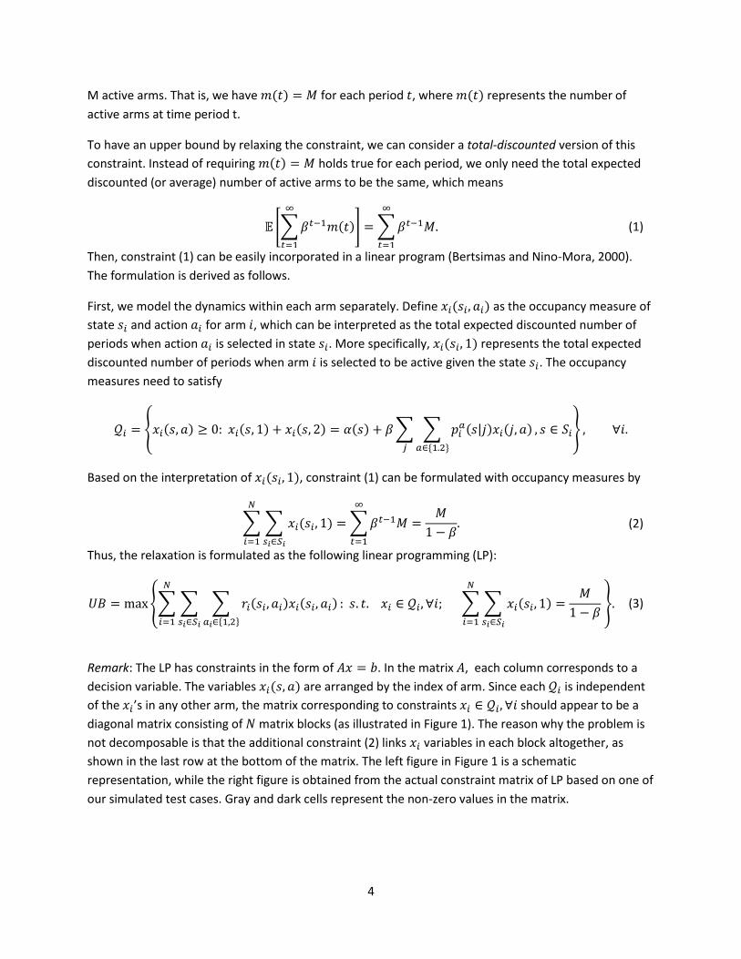
Remark: The LP has constraints in the form of . In the matrix , each column corresponds to a

decision variable. The variables are arranged by the index of arm. Since each is independent

of the ’s in any other arm, the matrix corresponding to constraints should appear to be a

diagonal matrix consisting of matrix blocks (as illustrated in Figure 1). The reason why the problem is

not decomposable is that the additional constraint (2) links variables in each block altogether, as

shown in the last row at the bottom of the matrix. The left figure in Figure 1 is a schematic

representation, while the right figure is obtained from the actual constraint matrix of LP based on one of

our simulated test cases. Gray and dark cells represent the non-zero values in the matrix.

5

Figure 1. Representation of the LP constraint matrix.

3 Heuristic index policies and algorithms Generalized from the Gittins index policy, a general index policy means that we select the arms with the

largest/smallest indices at each period. Then, one large decision problem for arms is reduced to

small problems for each individual arm separately, which makes the computation much more tractable.

For some problem instances, the index that has a good performance may reveal some intuitive insights

of the problem itself. Of course, this decomposition will results in some loss in the optimality. The next

question is that how to design the index with performance as close to the optimal as possible.

3.1 The Whittle index The Whittle index was originally proposed for the time-average reward problem in Whittle (1988) [3].

Glazebrook et al. (2006) [8] provided the formulation for the total discounted reward problem following

the same idea of the original Whittle index.

The derivation of Whittle index is based on the notion of passive subsidy , which means that an arm

will receive a subsidy W (possible to be negative) if it is passive. That is, the passive reward is

now replaced by for each . For each arm , we define the subsidy-W problem with

following optimality equation (we suppress the arm index in the subscript for simplicity):

{ ∑ |

∑ |

}

The value function now depends on the value of subsidy W. Then the Whittle index is

defined by

{ ∑ |

∑ |

}

In other words, the Whittle index of state can be interpreted as the subsidy such that being active and

passive are indistinguishable in the subsidy-W problem.

Although some studies established the closed-form solution of the Whittle index in specific application

problems, no generic algorithm to compute the Whittle index numerically is directly available from the

6

literature. To be able to test the performance of the Whittle index policy and compare with other

policies on our simulated cases, we propose the following algorithm to compute the Whittle index

numerically.

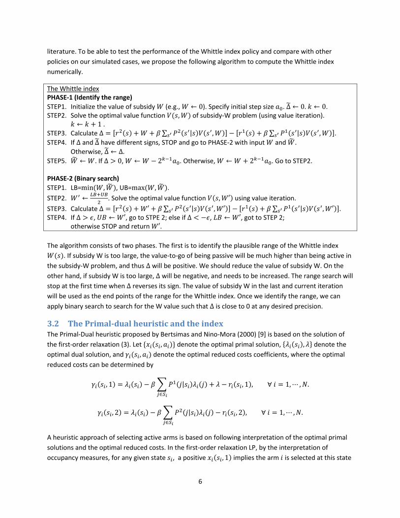
The Whittle index PHASE-1 (Identify the range)

STEP1. Initialize the value of subsidy (e.g., ). Specify initial step size . ̃ . STEP2. Solve the optimal value function of subsidy-W problem (using value iteration).

. STEP3. Calculate [ ∑ | ] [ ∑ | ].

STEP4. If and ̃ have different signs, STOP and go to PHASE-2 with input and ̃.

Otherwise, ̃

STEP5. ̃ . If , . Otherwise, . Go to STEP2. PHASE-2 (Binary search)

STEP1. LB= ̃ , UB= ̃ .

STEP2.

. Solve the optimal value function using value iteration.

STEP3. Calculate [ ∑ | ] [ ∑ | ]. STEP4. If , , go to STPE 2; else if , , got to STEP 2;

otherwise STOP and return .

The algorithm consists of two phases. The first is to identify the plausible range of the Whittle index

. If subsidy W is too large, the value-to-go of being passive will be much higher than being active in

the subsidy-W problem, and thus will be positive. We should reduce the value of subsidy W. On the

other hand, if subsidy W is too large, will be negative, and needs to be increased. The range search will

stop at the first time when reverses its sign. The value of subsidy W in the last and current iteration

will be used as the end points of the range for the Whittle index. Once we identify the range, we can

apply binary search to search for the W value such that is close to 0 at any desired precision.

3.2 The Primal-dual heuristic and the index The Primal-Dual heuristic proposed by Bertsimas and Nino-Mora (2000) [9] is based on the solution of

the first-order relaxation (3). Let denote the optimal primal solution, denote the

optimal dual solution, and denote the optimal reduced costs coefficients, where the optimal

reduced costs can be determined by

∑ |

∑ |

A heuristic approach of selecting active arms is based on following interpretation of the optimal primal

solutions and the optimal reduced costs. In the first-order relaxation LP, by the interpretation of

occupancy measures, for any given state , a positive implies the arm is selected at this state

7

with positive probability, which can be regarded as a candidate active arm. The optimal reduced cost

is the rate of decrease in the objective value as the value of increases by 1 unit,

which essentially describes the “penalty” of having a high value of .

Next, we can select active arms according to following scheme:

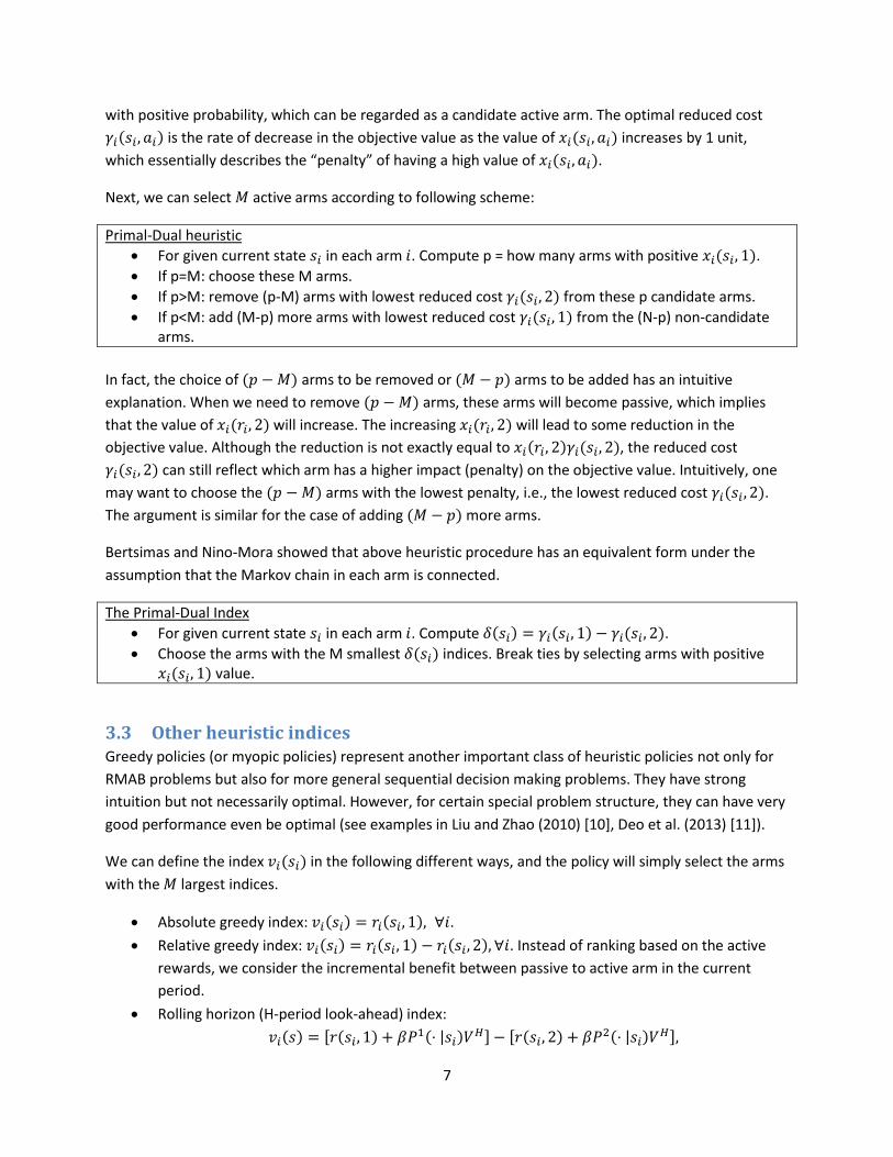
Primal-Dual heuristic

For given current state in each arm . Compute p = how many arms with positive .

If p=M: choose these M arms.

If p>M: remove (p-M) arms with lowest reduced cost from these p candidate arms.

If p<M: add (M-p) more arms with lowest reduced cost from the (N-p) non-candidate arms.

In fact, the choice of arms to be removed or arms to be added has an intuitive

explanation. When we need to remove arms, these arms will become passive, which implies

that the value of will increase. The increasing will lead to some reduction in the

objective value. Although the reduction is not exactly equal to , the reduced cost

can still reflect which arm has a higher impact (penalty) on the objective value. Intuitively, one

may want to choose the arms with the lowest penalty, i.e., the lowest reduced cost .

The argument is similar for the case of adding more arms.

Bertsimas and Nino-Mora showed that above heuristic procedure has an equivalent form under the

assumption that the Markov chain in each arm is connected.

The Primal-Dual Index

For given current state in each arm . Compute .

Choose the arms with the M smallest indices. Break ties by selecting arms with positive value.

3.3 Other heuristic indices Greedy policies (or myopic policies) represent another important class of heuristic policies not only for

RMAB problems but also for more general sequential decision making problems. They have strong

intuition but not necessarily optimal. However, for certain special problem structure, they can have very

good performance even be optimal (see examples in Liu and Zhao (2010) [10], Deo et al. (2013) [11]).

We can define the index in the following different ways, and the policy will simply select the arms

with the largest indices.

Absolute greedy index: .

Relative greedy index: . Instead of ranking based on the active

rewards, we consider the incremental benefit between passive to active arm in the current

period.

Rolling horizon (H-period look-ahead) index:

[ | ] [ |

]

8

in which represents the optimal value function for the next periods. Instead of comparing

the incremental benefit in the current period, we will compare the overall incremental benefits

over the next periods.

4 Numerical results: simulated cases

4.1 Experimental Design There are 5 key questions we would like this study to address:

1. How do different policies compare under different problem structures?

2. How do different policies compare under different problem sizes?

3. Does discount factor play a significant role in algorithm performance?

4. Does time horizon play a significant role in algorithm performance?

5. Can a rolling horizon look-ahead policy improve the relative greedy policy?

To answer these questions, we will use a series of numerical simulations. In all cases, we assume the

arms are not identical; that is, each arm has different rewards and transition matrices. We also assume

the reward for activating an arm is greater than the reward for leaving the arm passive. This assumption

is common in most modeling frameworks. For each arm in each state, we generate two uniform (0,1)

random variables and set the maximum of these to be the active reward, and the minimum to be the

passive reward. Except for the special cases described below, the active and passive transition matrices

of each arm are uniformly sampled from the space of all transition matrices. We do this sampling via

the standard procedure: For each row of the transition matrix, we generate |S| exponential (1) random

variables and scale each by their sum so that each entry is nonnegative and the row sums to 1. Thus the

transition matrices are irreducible aperiodic and pij > 0 for all i, j. Except where mentioned, we consider

the infinite horizon case with a discount factor of 0.9.

To answer question 1, we consider 4 special structures the transition matrices can take on:

a) The uniform case described above

b) The less connected (LC) case

In this structure, each state can only transition to adjacent states. Namely, state 1 can transition

to state 1 or 2, state 2 can transition to state 2 or 3, and so on.

c) Increasing failure rate (IFR) case

For both the active and passive transition matrices,

∑ |

| |

is non-decreasing in i for all arms. Together with non-increasing rewards in the state space, this

condition implies higher states are more likely to deteriorate faster. This modeling framework is

useful for many problems such as machine maintenance and health care: once a machine starts

breaking, it is more likely to continue deteriorating to worse conditions.

d) P1 is stochastically smaller than P2 (P1 SS P2)

9

A form of stochastic ordering, this condition imposes

∑ | ∑ | | |

| |

| |

for every arm. We also impose non-increasing rewards in the state space, so this condition says

we are more likely to stay in a lower, more beneficial state under the active transition matrix

than under the passive transition matrix.

To answer question 2, we will first fix N and M and increase S, then fix S and M and increase N. For

question 3, we consider a range of discount factors from 0.4 to 0.99. In question 4, we consider

different finite horizons ranging from 10 to 300, and compare this to the infinite horizon. For question

5, we consider 2, 5, 10, and 50 period look-ahead policies for both the uniform and less connected case.

When the problem instance is small and we can solve the dynamic programming problem to optimality,

we compute this optimal solution, evaluate the optimal value exactly, and compare each algorithm’s

performance to optimality. For larger instances, we compute the Lagrange upper bound, evaluate each

policy via Monte-Carlo simulation, and compare the performance to the upper bound.

4.2 Results

1. How do different policies compare under different problem structures?

Figure 2 demonstrates the results of the numerical experiments for question 1. Since this is a relatively

small problem size, we can solve each to optimality with dynamic programming. Each cluster of bars

represents a particular algorithm, and each bar within the cluster represents the percentage gap from

optimality of that algorithm on a specified problem structure.

The first observation we draw from these results is that across all problem structures, Whittle index and

the primal dual method are the most effective. For all instances except for the less connected case,

both algorithms perform within 0.1% of optimality. We also observe the absolute greedy policy

performs unacceptably poorly in all structures. For the increasing failure rate structure, the absolute

greedy policy performs only marginally better than the baseline policy of completely random choice of

arms.

Our next observation is that all algorithms except for primal dual perform substantially worse on the less

connected case than for any other structure. This can be interpreted as the algorithms failing to capture

the special fact that the chain cannot transition between any arbitrary pair of states. Whittle index only

considers the value function of adjacent states, and the greedy policy does not consider any future

progression, so both perform poorly when the chain may not quickly reach an advantageous state.

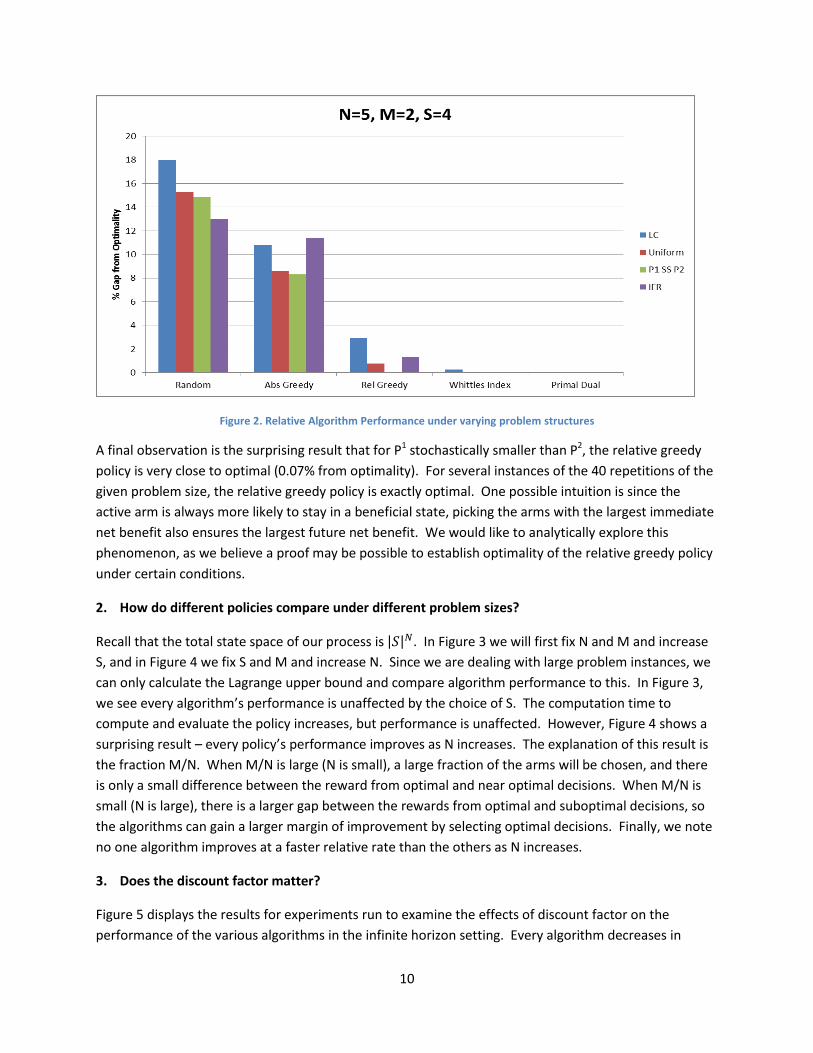
10

Figure 2. Relative Algorithm Performance under varying problem structures

A final observation is the surprising result that for P1 stochastically smaller than P2, the relative greedy

policy is very close to optimal (0.07% from optimality). For several instances of the 40 repetitions of the

given problem size, the relative greedy policy is exactly optimal. One possible intuition is since the

active arm is always more likely to stay in a beneficial state, picking the arms with the largest immediate

net benefit also ensures the largest future net benefit. We would like to analytically explore this

phenomenon, as we believe a proof may be possible to establish optimality of the relative greedy policy

under certain conditions.

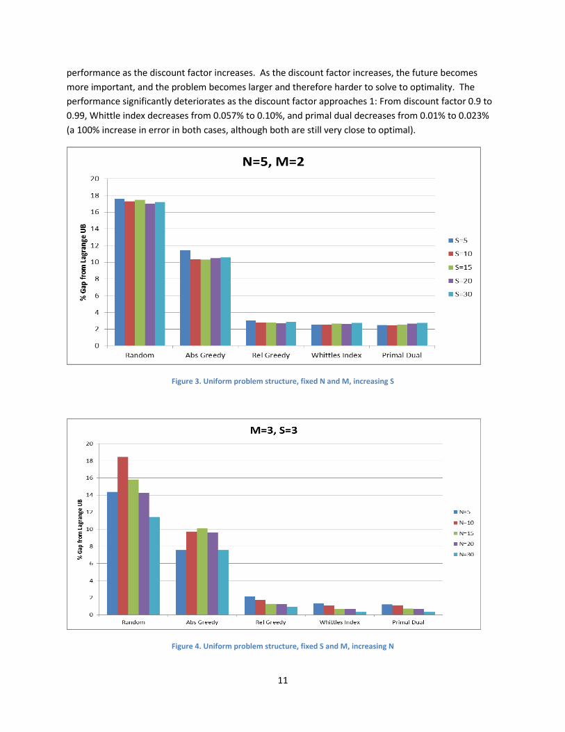
2. How do different policies compare under different problem sizes?

Recall that the total state space of our process is | | . In Figure 3 we will first fix N and M and increase

S, and in Figure 4 we fix S and M and increase N. Since we are dealing with large problem instances, we

can only calculate the Lagrange upper bound and compare algorithm performance to this. In Figure 3,

we see every algorithm’s performance is unaffected by the choice of S. The computation time to

compute and evaluate the policy increases, but performance is unaffected. However, Figure 4 shows a

surprising result – every policy’s performance improves as N increases. The explanation of this result is

the fraction M/N. When M/N is large (N is small), a large fraction of the arms will be chosen, and there

is only a small difference between the reward from optimal and near optimal decisions. When M/N is

small (N is large), there is a larger gap between the rewards from optimal and suboptimal decisions, so

the algorithms can gain a larger margin of improvement by selecting optimal decisions. Finally, we note

no one algorithm improves at a faster relative rate than the others as N increases.

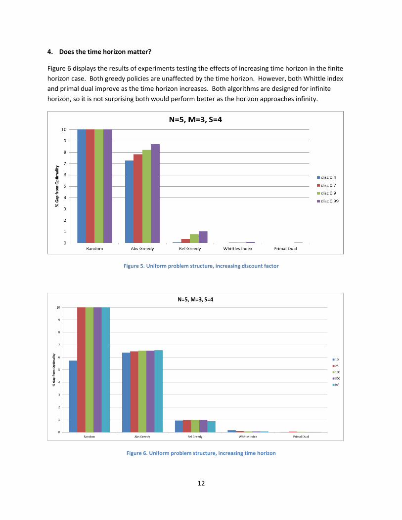
3. Does the discount factor matter?

Figure 5 displays the results for experiments run to examine the effects of discount factor on the

performance of the various algorithms in the infinite horizon setting. Every algorithm decreases in

11

performance as the discount factor increases. As the discount factor increases, the future becomes

more important, and the problem becomes larger and therefore harder to solve to optimality. The

performance significantly deteriorates as the discount factor approaches 1: From discount factor 0.9 to

0.99, Whittle index decreases from 0.057% to 0.10%, and primal dual decreases from 0.01% to 0.023%

(a 100% increase in error in both cases, although both are still very close to optimal).

Figure 3. Uniform problem structure, fixed N and M, increasing S

Figure 4. Uniform problem structure, fixed S and M, increasing N

12

4. Does the time horizon matter?

Figure 6 displays the results of experiments testing the effects of increasing time horizon in the finite

horizon case. Both greedy policies are unaffected by the time horizon. However, both Whittle index

and primal dual improve as the time horizon increases. Both algorithms are designed for infinite

horizon, so it is not surprising both would perform better as the horizon approaches infinity.

Figure 5. Uniform problem structure, increasing discount factor

Figure 6. Uniform problem structure, increasing time horizon

13

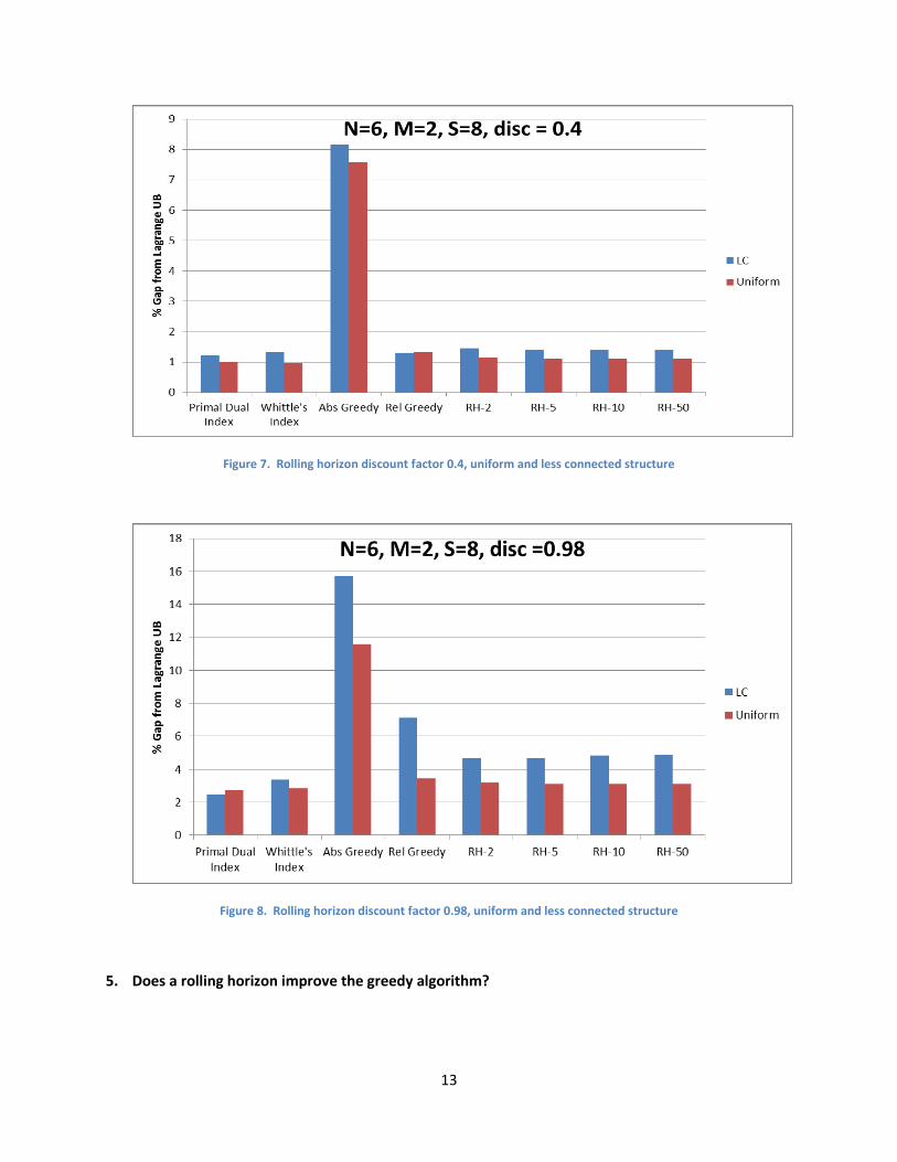
Figure 7. Rolling horizon discount factor 0.4, uniform and less connected structure

Figure 8. Rolling horizon discount factor 0.98, uniform and less connected structure

5. Does a rolling horizon improve the greedy algorithm?

14

and Figure 8 display the results of experiments testing whether a rolling horizon look-ahead policy can

improve the relative greedy policy. When the discount factor is low, as seen in table 6, a look-ahead

policy provides no benefit in either the uniform or less connected case. As previously discussed, for

such a low discount factor the future contribution to the total discounted reward is negligible compared

to the current period, so a look-ahead policy does not contribute much value. As the discount factor

increases, a look-ahead policy does gain improvement over the relative greedy policy. In table 7, the

discount factor is 0.98 and we see an improvement of the 2 step look-ahead policy in both the uniform

and less connected cases. The improvement is meager in the uniform case (8% relative improvement)

but significant in the less connected case (34% relative improvement). This agrees with our previous

result that greedy policies perform poorly on the less connected case because they fail to consider the

future development of the chain. We see no further improvement by looking more than 2 periods into

the future, implying a 3 or more step look-ahead policy expends more computational effort but does not

return a better solution. Finally, it should be noted that this 2 step look-ahead policy still performs

worse than the Whittle index and primal dual policy for both problem structures.

4.3 Validation of algorithm implementation All algorithms for policies construction and evaluation are implemented in MATLAB©. The first-order

relaxation LP is solved by calling the CPLEX library for MATLAB. Experiments are run on the Condor

Cluster of ISyE.

To validate the algorithm implementation, we have checked:

Policy evaluation: For small instances, the exact value function can be evaluated based on the

value iteration of equivalent MDP model. The results are very close to those based on the

Monte-Carlo simulation approach.

MDP and Whittle index policy: For small cases, MDP always provides the optimal objective

value. Whittle index can be reduced to Gittins index when passive arms are frozen (i.e., no

transition and no rewards). Gittins index is proven to be optimal when only one arm is activated

each time. That is, Whittle index can be optimal when passive arms are frozen and . We

test the two algorithms in simulated cases with different problem size, and observe that the

objective values of two algorithms are always identical in such condition. When becomes 2,

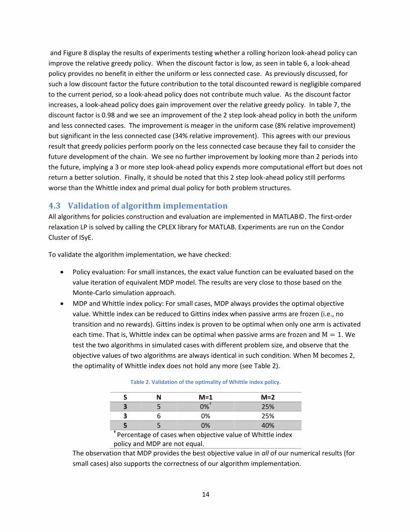
the optimality of Whittle index does not hold any more (see Table 2).

Table 2. Validation of the optimality of Whittle index policy.

S N M=1 M=2

3 5 0%† 25%

3 6 0% 25%

5 5 0% 40% † Percentage of cases when objective value of Whittle index policy and MDP are not equal.

The observation that MDP provides the best objective value in all of our numerical results (for

small cases) also supports the correctness of our algorithm implementation.

15

5 Application: Capacity allocation problem In this section, we will test and compare different algorithms and policies on a real application problem.

The objective is twofold. First, we will see how real problem can be modeled as an RMAB problem, and

know about the challenge of solving the RMAB of a real application size. Second, we will apply and

compare the performance of different policies (with some not included in the original paper).

The clinical capacity allocation problem (Deo et al. (2013) [11]) is about how to deliver the school-based

asthma care for children given the capacity constraint. A healthcare program visits a school every

month, and provides treatment to children with asthma. However, the capacity of

appointment/treatment during each visit is limited. Patients who have received treatment will improve

their health state while those without treatment may progress to worse state. Given the limited capacity

and disease dynamics, the objective is to maximize the total benefit of the community over two years.

Within the framework of RMAB, this problem can be modeled as follows:

N arms: number of total patients (typically ~ 50 patients).

M arms: capacity, the available slots in the van during each visit (typically ~ 10-15 patients).

: State space for each patient. In the model, each patient has (1) health state at the last

appointment and (2) time since the

last appointment (in month). Thus, .

: Transition matrix if the patient receives treatment:

( | )

where is the matrix of immediate transition after treatment, and is the matrix of disease

progression during one month.

: Transition matrix if the patient does not receive treatment:

( | )

and

: reward is the quality-adjusted life years (QALYs) at given state .

Remark: Not surprisingly, the problem size of the real application is far beyond being tractable. In

particular, the state space is | | . One may suggest using value function

approximation techniques to address the large state space since the states are only two-dimensional. In

fact, we can use simulation-based projected equation methods to approximate value function, instead

of calculating the exact value for each state. However, these approaches only resolve the challenges in

the policy evaluation step. In the policy improvement step, we need to find the maximum over (

) (in

the order of , (

) ) different actions, which is still prohibitively large for computation.

One possible approach is to approximate the policy function using a parametric model proposed in

Powell (2010) [12] . Current states and parameter are the inputs to the parametric model. Then, we

need to tune up the best parameter using stochastic optimization algorithms (e.g., random search,

stochastic approximation), instead of taking the maximum over an intractably large action space.

16

5.1 Numerical results In addition to the policies we introduced in Section 3, there are several more problem-specific policies to

be evaluated.

Fixed-duration policy. Physicians will recommend the next follow-up time based on patients’

health state (3 months for controlled state, and 1 month for uncontrolled states). The patients

who are due back in prior periods have the highest priority, and followed by those who are due

back in the current period.

H-N priority policy. It first prioritizes patients based on their health state observed in the last

appointment, and then breaks ties based on the time since the last appointment.

N-H priority policy. Similar to H-N priority policy but with a reversed order of prioritization.

No-schedule policy. No patients are scheduled and all follows the natural progression process.

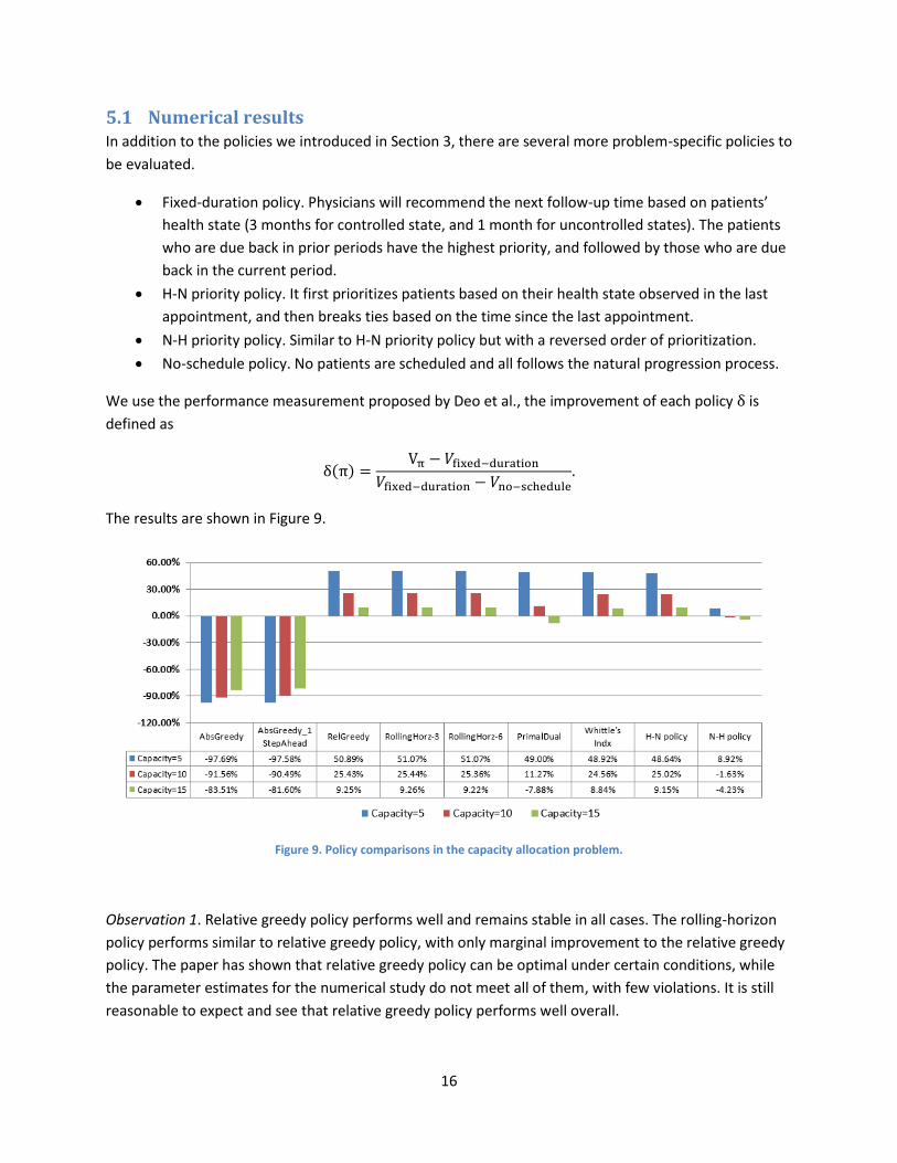
We use the performance measurement proposed by Deo et al., the improvement of each policy is

defined as

The results are shown in Figure 9.

Figure 9. Policy comparisons in the capacity allocation problem.

Observation 1. Relative greedy policy performs well and remains stable in all cases. The rolling-horizon

policy performs similar to relative greedy policy, with only marginal improvement to the relative greedy

policy. The paper has shown that relative greedy policy can be optimal under certain conditions, while

the parameter estimates for the numerical study do not meet all of them, with few violations. It is still

reasonable to expect and see that relative greedy policy performs well overall.

17

Observation 2. The Whittle index policy performs well and very close to the relative greedy policy.

However, it takes 1.5-3 hours to compute all Whittle indices for each state of each arm (

indices in total). As a generic heuristic index policy independent of problem structure, the Whittle

index policy has demonstrated its robustness of good performance in all tests that we have done in this

study.

Observation 3. Improvement reduces as the capacity becomes less restrictive. This finding is in line with

those based on the simulated cases in Section 4.2. As M/N becomes larger, the relative difference

between the best selection and the second best selection can be less significant.

Observation 4. As capacity increases, the performance of the primal-dual index policy degrades

significantly. We speculate that it may be because that the first-order relaxation LP used to compute the

primal-dual index is essentially an infinite horizon problem. We use a large discount factor 0.99 which

makes the model takes more care of future rewards. However, the capacity allocation problem is only

evaluated for 24 periods (2 years). This disconnect between the settings of the policy and the problem

may make the primal-dual index policy behave poorly.

6 Conclusion From our numerical experiments, we have demonstrated Whittle index and the primal dual policy both

work efficiently in all cases. They provide solutions within 1% of optimality when we know the exact

solution, and within 5% of the Lagrange upper bound when we cannot calculate the optimal solution.

The computation time of the policy is only seconds for even the largest problems we tested, although

evaluating the solution may still be costly. These algorithms remain the best choice for all problem sizes

and all structures, although the relative greedy policy is close to optimal when P1 is stochastically smaller

than P2. Both Whittle index and the primal dual policy perform better when the time horizon is large or

infinite. All algorithms perform more poorly when the discount factor is large, due to the added

complexity of the optimization.

In the real application, we have seen the relative greedy policy perform very close to optimal, as

dictated by the special structure of the problem. The Whittle index was very expensive to compute, and

performed less well than the greedy policy. Consistent with our results from the numerical experiments,

we found the primal dual policy did not perform well because it is evaluated only on a relatively small

time horizon.

Reference 1. Jones, D.M. and J.C. Gittins, A dynamic allocation index for the sequential design of experiments.

1972: University of Cambridge, Department of Engineering. 2. Gittins, J.C. and D.M. Jones, A dynamic allocation index for the discounted multiarmed bandit

problem. Biometrika, 1979. 66(3): p. 561-565. 3. Whittle, P., Restless bandits: Activity allocation in a changing world. Journal of applied

probability, 1988: p. 287-298.

18

4. Weber, R.R. and G. Weiss, On an index policy for restless bandits. Journal of Applied Probability, 1990: p. 637-648.

5. Papadimitriou, C.H. and J.N. Tsitsiklis, The complexity of optimal queuing network control. Mathematics of Operations Research, 1999. 24(2): p. 293-305.

6. Ansell, P., et al., Whittle's index policy for a multi-class queueing system with convex holding costs. Mathematical Methods of Operations Research, 2003. 57(1): p. 21-39.

7. Glazebrook, K.D., H. Mitchell, and P. Ansell, Index policies for the maintenance of a collection of machines by a set of repairmen. European Journal of Operational Research, 2005. 165(1): p. 267-284.

8. Glazebrook, K., D. Ruiz-Hernandez, and C. Kirkbride, Some indexable families of restless bandit problems. Advances in Applied Probability, 2006: p. 643-672.

9. Bertsimas, D. and J. Niño-Mora, Restless bandits, linear programming relaxations, and a primal-dual index heuristic. Operations Research, 2000. 48(1): p. 80-90.

10. Liu, K. and Q. Zhao, Indexability of restless bandit problems and optimality of Whittle index for dynamic multichannel access. Information Theory, IEEE Transactions on, 2010. 56(11): p. 5547-5567.

11. Deo, S., et al., Improving Health Outcomes Through Better Capacity Allocation in a Community-Based Chronic Care Model. Operations Research, 2013. 61(6): p. 1277-1294.

12. Powell, W.B., Approximate Dynamic Programming: Solving the curses of dimensionality. Vol. 703. 2007: John Wiley & Sons.