UvA-DARE is a service provided by the library of the University of Amsterdam (http://dare.uva.nl)

UvA-DARE (Digital Academic Repository)

Responses to the incidental parameter problem

Pua, A.A.Y.

Link to publication

Citation for published version (APA):Pua, A. A. Y. (2016). Responses to the incidental parameter problem

General rightsIt is not permitted to download or to forward/distribute the text or part of it without the consent of the author(s) and/or copyright holder(s),other than for strictly personal, individual use, unless the work is under an open content license (like Creative Commons).

Disclaimer/Complaints regulationsIf you believe that digital publication of certain material infringes any of your rights or (privacy) interests, please let the Library know, statingyour reasons. In case of a legitimate complaint, the Library will make the material inaccessible and/or remove it from the website. Please Askthe Library: http://uba.uva.nl/en/contact, or a letter to: Library of the University of Amsterdam, Secretariat, Singel 425, 1012 WP Amsterdam,The Netherlands. You will be contacted as soon as possible.

Download date: 31 Jul 2018

In recent years, we have seen an explosion of data collected fromindividuals, firms, or countries across short or long periods oftime. This type of data gives us an opportunity to study thedynamics of change while controlling for time-invariantunobserved heterogeneity. Unfortunately, this type ofheterogeneity, which is usually in the form of individual-specificfixed effects, creates problems for identification, estimation, andinference, especially if we continue to use default procedureswithout modification or without critical exploration. Thisdissertation revolves around a common theme – what practicesand methods can be considered appropriate responses to theincidental parameter problem in panel data models. Myapproach to research is firmly rooted in the examination ofempirical and theoretical practices so that we can come to anunderstanding of what we can and cannot do.

Andrew Adrian Yu Pua (1984) is no stranger to double degrees.He received a BA in Economics and a BSc in Accountancy fromDe La Salle University – Manila (DLSU). He also received amaster’s degree in mathematics from the same institution. Afteraround three years as a faculty member of DLSU, he traveled toEurope to commence postgraduate studies. With the support ofthe European Commission through the Erasmus Mundus scheme,he obtained an MSc Wirtschaftsmathematik from UniversitätBielefeld and a Master Mathématiques Appliquées à l’Economieet à la Finance from the Université Paris 1 Panthéon-Sorbonne.Now, with the support of the same commission, he is about toreceive his PhD in Economics from both the University ofAmsterdam and the Université Catholique de Louvain.

Res

pon

ses

toth

eIn

cide

nta

lPar

amet

erPr

oble

m

Responses to theIncidental Parameter

Problem

Andrew Adrian Yu Pua

Responses to the Incidental Parameter Problem

Dit proefschrift is tot stand gekomen in het kader van EDE-EM (European Doctorate inEconomics – Erasmus Mundus), met als doel het behalen van een gezamenlijk doctoraat. Hetproefschrift is voorbereid aan de Faculteit Economie en Bedrijfskunde van de Universiteit vanAmsterdam en aan de Center for Operations Research and Econometrics van de UniversitéCatholique de Louvain.

La thèse a été préparée dans le cadre du programme doctoral européen EDE-EM (EuropeanDoctorate in Economics – Erasmus Mundus). Cette thèse a été préparée conjointment auFaculteit Economie en Bedrijfskunde, Universiteit van Amsterdam et au Center for OperationsResearch and Econometrics, Université Catholique de Louvain.

This thesis has been written within the framework of the EDE-EM (European Doctorate inEconomics – Erasmus Mundus), with the purpose of obtaining a joint doctorate degree. Thethesis was prepared in the Faculty of Economics and Business at the University of Amsterdamand in the Center for Operations Research and Econometrics at the Université Catholique deLouvain.

Layout and cover design by Andrew Adrian Yu Pua

ISBN 978-94-91030-84-0NUR 916

c© Andrew Adrian Yu Pua, 2016

All rights reserved. Without limiting the rights under copyright reserved above, no part ofthis book may be reproduced, stored in, or introduced into a retrieval system, or transmitted,in any form or by any means (electronic, mechnical, photocopying, recording, or otherwise)without the written permission of both the copyright owner and author of the book.

RESPONSES TO THE INCIDENTAL PARAMETER PROBLEM

ACADEMISCH PROEFSCHRIFT

ter verkrijging van de graad van doctor

aan de Universiteit van Amsterdam

op gezag van de Rector Magnificus

prof. dr. D. C. van den Boom

ten overstaan van een door het College voor Promoties ingestelde

commissie, in het openbaar te verdedigen in de Agnietenkapel

op donderdag 10 maart 2016, te 14:00 uur

door

Andrew Adrian Yu Pua

geboren te Manilla, Filipijnen

Promotiecommissie:

Promotor: Prof. dr. H. P. Boswijk Universiteit van AmsterdamProf. dr. S. van Bellegem Université Catholique de Louvain

Copromotor: Dr. M. J. G. Bun Universiteit van AmsterdamOverige leden: Prof. dr. G. Dhaene Katholieke Universiteit Leuven

Dr. K. J. van Garderen Universiteit van AmsterdamDr. N. P. A. van Giersbergen Universiteit van AmsterdamProf. dr. C. M. Hafner Université Catholique de LouvainProf. dr. S. Khan Duke UniversityProf. dr. F. R. Kleibergen Universiteit van Amsterdam

Faculteit: Economie en Bedrijfskunde

Acknowledgements

I acknowledge the funding and support of the Education, Audiovisual and Cul-ture Executive Agency (EACEA) of the European Union during my stay in Europefrom September 2009 to August 2014. The agency financed both my scholarshipfor the Erasmus Mundus Master Course QEM and my fellowship for the ErasmusMundus Joint Doctorate EDEEM. I also thank my promotor Peter Boswijk for offer-ing a teaching gig that allowed me to stay at the University of Amsterdam until 1February 2016.

I would like to thank six sets of people: my family, my friends, my colleagues,the participants at talks, the support staff, and the nameless future reader.

First, I spent most of my time with colleagues at the University of Amsterdam(UvA) and at the Center for Operations Research and Econometrics (CORE). I thankmy promotors, Peter Boswijk and Sébastien van Bellegem, for all the talks, discus-sions, and the candidness. I also thank Maurice Bun for his patience in going throughthe manuscript. They have decided to trust me and I hope I was able to deliver. Ialso thank my doctoral committee for taking the time to read my manuscript. Theircomments have been useful in rethinking about the approaches I considered in thethesis. Let me also single out members of my doctoral committee – Geert Dhaene,Shakeeb Khan, and Frank Kleibergen, for their support in my job search.

Second, I thank all the people who have attended my talks or listened to my ideas(either forced or of their own volition). Let me single out people who have offeredsome perspective through their comments – Luc Bauwens, Stéphane Bonhomme, Si-mon Broda, Martin Carree, Pavel Cížek, Geert Dhaene, Firmin Doko Tchatoka, Jian-qing Fan, Kees Jan van Garderen, Noud van Giersbergen, Refet Gürkaynak, ChristianHafner, Harry Haupt, Arturas Juodis, Shakeeb Khan, Jan Kiviet, Frank Kleibergen,Thierry Magnac, Michael Massmann, Salvador Navarro, Serena Ng, Cavit Pakel, DalePoirier, Renata Rabovic, Douglas Steigerwald, Martin Weidner, Frank Windmeijer,and Jeffrey Wooldridge. I also thank Roy van der Weide for sharing the data used inChapter 5.

Third, I thank all my friends for their support, even if I am usually not around.Most of my friends are back home in the Philippines and I thank them for makingmy return home so much fun. I also thank the EDEEM cohort for their help in ad-ministrative matters.

Fourth, the support staff at UvA and CORE have made smooth transitions possi-ble. Arnold van Meteren was one of my earliest contacts at UvA. He was responsiblefor facilitating my long-stay visa application in the Netherlands. José Kiss was veryhelpful in facilitating accommodation in Amsterdam and registration at the UvA.Kees Nieuwland made office life smoother by being there for computer-related is-sues. Jolanda Vroons also took his place as IT liaison and was very quick to respond.Evelien Brink, Ana Colic, Wilma de Kruijf, and Robert Helmink are always there to

v

help whenever I would need assistance. Marc van Steekelenburg has been helpfulin dealing with renewing my residence permit. Catherine Germain is possibly one ofthe best multi-taskers I have ever seen in action. She helped in smoothing out mymove to Belgium, dealing with French-speaking authorities, and expediting the finalactivities of the dissertation defense phase. Marie-Hélène Chassagne has also beenvery helpful with these final activities as well. Raphaël Tursis was one of the nicer ITguys I have met. I also thank Caroline Dutry, the only support staff at the coordinat-ing institution of the doctoral programme, for dealing with both administrative andfinance-related issues. The support staff is really the heart of any institution!

Fifth, I thank the reader of this thesis. I hope you enjoy reading this work just asI have enjoyed (though not without heartbreak) working on it. In case you did notnotice, the last few pages of the dissertation are blanks meant for notes.

Finally, I thank my mother for understanding the nature of what I have beendoing for the past years, despite her initial hesitations. I thank my brother and sisterfor being there with my mother in my absence. Although infuriating at times, I wouldlike to thank the cats and our lone dog back in our house, as they have stabilized thehousehold. I thank my better half Stephanie for being one of the constants in mylife.

vi

Contents

1 Introduction 11.1 The promise of panel data . . . . . . . . . . . . . . . . . . . . . . . . . . . . 11.2 Sketching some of the arguments . . . . . . . . . . . . . . . . . . . . . . . 41.3 How should we respond? . . . . . . . . . . . . . . . . . . . . . . . . . . . . 18

2 On IV estimation of a dynamic linear probability model with fixed effects 212.1 Introduction . . . . . . . . . . . . . . . . . . . . . . . . . . . . . . . . . . . . 212.2 A situation where the LPM is a good idea . . . . . . . . . . . . . . . . . . 232.3 Main results . . . . . . . . . . . . . . . . . . . . . . . . . . . . . . . . . . . . 25

2.3.1 The case of three time periods . . . . . . . . . . . . . . . . . . . . . 252.3.2 Large-T case . . . . . . . . . . . . . . . . . . . . . . . . . . . . . . . 28

2.4 Practical implications . . . . . . . . . . . . . . . . . . . . . . . . . . . . . . . 302.5 Concluding remarks . . . . . . . . . . . . . . . . . . . . . . . . . . . . . . . 342.6 Appendix . . . . . . . . . . . . . . . . . . . . . . . . . . . . . . . . . . . . . . 34

3 Simultaneous equations models for discrete outcomes: Coherence andcompleteness using panel data 393.1 Introduction . . . . . . . . . . . . . . . . . . . . . . . . . . . . . . . . . . . . 393.2 A stylized example . . . . . . . . . . . . . . . . . . . . . . . . . . . . . . . . 41

3.2.1 Coherence and completeness . . . . . . . . . . . . . . . . . . . . . 413.2.2 Why a cross section is not enough . . . . . . . . . . . . . . . . . . 453.2.3 Why panel data may be useful . . . . . . . . . . . . . . . . . . . . 47

3.3 The model . . . . . . . . . . . . . . . . . . . . . . . . . . . . . . . . . . . . . 483.3.1 Background . . . . . . . . . . . . . . . . . . . . . . . . . . . . . . . . 483.3.2 Identification . . . . . . . . . . . . . . . . . . . . . . . . . . . . . . . 503.3.3 Estimation and inference . . . . . . . . . . . . . . . . . . . . . . . . 54

3.4 Revisiting the results of HI (1995; 2007) . . . . . . . . . . . . . . . . . . 573.4.1 Similarities and differences . . . . . . . . . . . . . . . . . . . . . . 573.4.2 Results . . . . . . . . . . . . . . . . . . . . . . . . . . . . . . . . . . . 58

3.5 Concluding remarks . . . . . . . . . . . . . . . . . . . . . . . . . . . . . . . 633.6 Appendix . . . . . . . . . . . . . . . . . . . . . . . . . . . . . . . . . . . . . . 64

vii

4 Estimation and inference in dynamic nonlinear fixed effects panel datamodels by projection 734.1 Introduction . . . . . . . . . . . . . . . . . . . . . . . . . . . . . . . . . . . . 734.2 The projection approach . . . . . . . . . . . . . . . . . . . . . . . . . . . . 76

4.2.1 Concept . . . . . . . . . . . . . . . . . . . . . . . . . . . . . . . . . . 764.2.2 Implications . . . . . . . . . . . . . . . . . . . . . . . . . . . . . . . . 784.2.3 Computation . . . . . . . . . . . . . . . . . . . . . . . . . . . . . . . 804.2.4 Examples . . . . . . . . . . . . . . . . . . . . . . . . . . . . . . . . . 83

4.3 Simulations . . . . . . . . . . . . . . . . . . . . . . . . . . . . . . . . . . . . . 874.4 Concluding remarks . . . . . . . . . . . . . . . . . . . . . . . . . . . . . . . 924.5 Appendix . . . . . . . . . . . . . . . . . . . . . . . . . . . . . . . . . . . . . . 93

5 The role of sparsity in panel data models 1095.1 Introduction . . . . . . . . . . . . . . . . . . . . . . . . . . . . . . . . . . . . 1095.2 Panel lasso for the linear model . . . . . . . . . . . . . . . . . . . . . . . . 111

5.2.1 Setup and notation . . . . . . . . . . . . . . . . . . . . . . . . . . . 1115.2.2 Estimation and inference . . . . . . . . . . . . . . . . . . . . . . . . 1145.2.3 Choice of regularization parameter . . . . . . . . . . . . . . . . . . 120

5.3 Monte Carlo . . . . . . . . . . . . . . . . . . . . . . . . . . . . . . . . . . . . 1225.4 Inequality and income growth . . . . . . . . . . . . . . . . . . . . . . . . . 1255.5 Concluding remarks . . . . . . . . . . . . . . . . . . . . . . . . . . . . . . . 1275.6 Appendix . . . . . . . . . . . . . . . . . . . . . . . . . . . . . . . . . . . . . . 129

6 Summary 135

Bibliography 137

Nederlandse Samenvatting (Summary in Dutch) 147

viii

Chapter 1

Introduction

1.1 The promise of panel data

In this chapter, I show through a series of examples that panel data offer researchersthree broad but sometimes competing advantages – estimating structural or commonparameters more precisely, allowing for dynamics and feedback, and control of time-invariant unobserved heterogeneity. I am working within usual panel data contextwhere the cross-sectional units i are independently sampled.

Let y ti = (yi1, . . . , yi t) and x t

i = (x i1, . . . , x i t) for i = 1, . . . , n and t = 1, . . . , T . Thevariable yi t is the outcome of interest and x i t is a vector of regressors – both of whichare observable. We are interested in the conditional distribution of the observablesy T

i given x Ti , which is indexed by a finite-dimensional parameter θ . Unfortunately,

the presence of the unobservable αi , which is an individual-specific effect capturingtime-invariant unobserved heterogeneity potentially correlated with the regressors,obscures our ability to estimate and make inferences about θ . To see this, considera prototypical panel data model where the previously mentioned elements can befound in the following integral equation, i.e.,

f y|x

y Ti |x

Ti ;θ

=ˆ

f y|x ,α

y Ti |x

Ti ,αi;θ

fα|x

αi |x Ti

dαi ,

where f y|x ,α

y Ti |x

Ti ,αi;θ

is a conditional model and fα|x

αi |x Ti

is the distributionof time-invariant unobserved heterogeneity.

The integral equation can be modified can allow for x to be strictly exogenousand for y to have dynamics (where yi1 plays the role of the initial condition), i.e.,

f

yiT , . . . , yi2|yi1, x Ti ;θ

=ˆ

f1

yiT , . . . , yi2|yi1, x Ti ,αi;θ

f2

αi |yi1, x Ti

dαi ,

1

where the integrand is given by

f1

·|yi1, x Ti ,αi;θ

= gT

yiT |x Ti , y T−1

i ,αi

× . . .× g2

yi2|x Ti , yi1,αi

.

The integral equation can also be modified to allow for x to have feedback, i.e.,

f (yiT , . . . , yi2, x iT , . . . , x i2|yi1, x i1;θ )

=ˆ

f1 (yiT , . . . , yi2, x iT , . . . , x i2|yi1, x i1,αi;θ ) f2 (αi |yi1, x i1) dαi ,

where the integrand is given by

f1 (·|yi1, x i1,αi;θ ) = gT

yiT |x Ti , y T−1

i ,αi

hT

x iT |y T−1i , x T−1

i ,αi

× . . .

×g2

yi2|x2i , yi1,αi

h2 (x i2|yi1, x i1,αi) .

It is certainly possible for each of the terms of the above expression to be indexed bysome finite-dimensional parameter θ . Furthermore, it is also possible to have a multi-dimensional fixed effect αi . Note that having the time series dimension providesmore degrees of freedom for which to estimate θ but these degrees of freedom mayget consumed by considering more and more complex models, even if we retain fullyparametric specifications.

A large part of research in panel data econometrics adopts a fully parametricspecification for f y|x ,α while leaving fα|x unspecified (see the surveys by Chamber-lain (1984), Arellano and Honoré (2001), and Arellano and Bonhomme (2011)).Leaving fα|x unspecified is at the core of the fixed-effects approach because one hasto account for sources of heterogeneity not always observed by the econometrician.Since there is scarce guidance from economic theory as to the nature of heterogeneityobserved units should possess, we start with a widely used notion of heterogeneity– that any differences among observed units are relatively stable over time but areallowed to be correlated with the included regressors. Unfortunately, the presenceof individual-specific effects complicates the estimation of common parameters indynamic nonlinear fixed effects panel data models, as we shall see in the exam-ples in the next section. Alternatively, correlated random effects approaches, wheresome aspects of the distribution fα|x are specified, can be beneficial as discussed inExample 1.2.6. In practice, either we impose assumptions on the first and secondmoments of fα|x for linear models or we impose fully parametric assumptions on fα|xfor nonlinear models.

The conditional model with f y|x ,α fully specified can also be used as a startingpoint while treating the αi ’s as parameters to be estimated. In this case, Neymanand Scott (1948) call θ the structural parameter and αi the incidental parameter.The distinguishing feature of parametric statistical models with incidental parame-ters is the presence of a parameter αi that appears in only a finite number of proba-

2

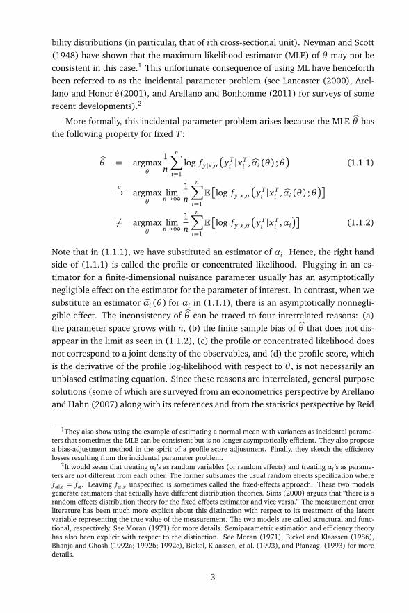
bility distributions (in particular, that of ith cross-sectional unit). Neyman and Scott(1948) have shown that the maximum likelihood estimator (MLE) of θ may not beconsistent in this case.1 This unfortunate consequence of using ML have henceforthbeen referred to as the incidental parameter problem (see Lancaster (2000), Arel-lano and Honoré (2001), and Arellano and Bonhomme (2011) for surveys of somerecent developments).2

More formally, this incidental parameter problem arises because the MLE bθ hasthe following property for fixed T :

bθ = argmaxθ

1n

n∑

i=1

log f y|x ,α

y Ti |x

Ti ,Òαi (θ ) ;θ

(1.1.1)

p→ argmax

θ

limn→∞

1n

n∑

i=1

E

log f y|x ,α

y Ti |x

Ti ,Òαi (θ ) ;θ

6= argmaxθ

limn→∞

1n

n∑

i=1

E

log f y|x ,α

y Ti |x

Ti ,αi

(1.1.2)

Note that in (1.1.1), we have substituted an estimator of αi . Hence, the right handside of (1.1.1) is called the profile or concentrated likelihood. Plugging in an es-timator for a finite-dimensional nuisance parameter usually has an asymptoticallynegligible effect on the estimator for the parameter of interest. In contrast, when wesubstitute an estimator Òαi (θ ) for αi in (1.1.1), there is an asymptotically nonnegli-gible effect. The inconsistency of bθ can be traced to four interrelated reasons: (a)the parameter space grows with n, (b) the finite sample bias of bθ that does not dis-appear in the limit as seen in (1.1.2), (c) the profile or concentrated likelihood doesnot correspond to a joint density of the observables, and (d) the profile score, whichis the derivative of the profile log-likelihood with respect to θ , is not necessarily anunbiased estimating equation. Since these reasons are interrelated, general purposesolutions (some of which are surveyed from an econometrics perspective by Arellanoand Hahn (2007) along with its references and from the statistics perspective by Reid

1They also show using the example of estimating a normal mean with variances as incidental parame-ters that sometimes the MLE can be consistent but is no longer asymptotically efficient. They also proposea bias-adjustment method in the spirit of a profile score adjustment. Finally, they sketch the efficiencylosses resulting from the incidental parameter problem.

2It would seem that treating αi ’s as random variables (or random effects) and treating αi ’s as parame-ters are not different from each other. The former subsumes the usual random effects specification wherefα|x = fα. Leaving fα|x unspecified is sometimes called the fixed-effects approach. These two modelsgenerate estimators that actually have different distribution theories. Sims (2000) argues that “there is arandom effects distribution theory for the fixed effects estimator and vice versa.” The measurement errorliterature has been much more explicit about this distinction with respect to its treatment of the latentvariable representing the true value of the measurement. The two models are called structural and func-tional, respectively. See Moran (1971) for more details. Semiparametric estimation and efficiency theoryhas also been explicit with respect to the distinction. See Moran (1971), Bickel and Klaassen (1986),Bhanja and Ghosh (1992a; 1992b; 1992c), Bickel, Klaassen, et al. (1993), and Pfanzagl (1993) for moredetails.

3

(2013), which contain some of the different likelihoods available in the literature)will tend to focus on directly addressing one of these four reasons.

Because the incidental parameter problem is difficult to handle for many non-linear panel models, some approaches that weaken the fixed-effects approach havebeen proposed. Typically, the search for consistent estimators of common parametersdepends on a set of auxiliary assumptions. Assumptions include, but are not limitedto, correlated random effects strategies where the αi ’s are drawn from a known fα|x(a particular approach involving sparsity is explored in Chapter 5), fixed-T or large-T bias corrections that exploit full specification of f y|x ,α (some of which are exploredfurther in Chapter 4), and approaches invoking discrete support for fα|x (exploredfurther in a simultaneous equations context in Chapter 3). The next four chapters ofthis dissertation provide specific theoretical or empirical situations for which theseauxiliary assumptions may be appropriate (or inappropriate as will be seen in Chap-ter 2). Before discussing the rest of the thesis, I first discuss the incidental parameterproblem in more detail using seven examples.

1.2 Sketching some of the arguments

In this section, I consider some examples that demonstrate the theoretical and prac-tical relevance of the incidental parameter problem along with some proposed solu-tions. Example 1.2.1 is the many normal means problem posed in Neyman and Scott(1948) where the parameter of interest is the common variance of the observations.The MLE in this example is inconsistent and model-specific solutions are proposedto remedy this inconsistency.

Example 1.2.2 reconsiders the solutions in Example 1.2.1 when both n, T →∞.Next, Example 1.2.3 is an illustration of the more general case where the O

T−1

incidental parameter bias is characterized so that we can pursue a general purposesolution. The model-specific nature of fixed-T solutions is further explored in Exam-ples 1.2.4 and 1.2.5. Sometimes these structural parameters are not of main interestand we want to determine how to recover average marginal effects. Example 1.2.6contains a discussion of how this can be accomplished in fixed-T and large-T sit-uations. Finally, I consider situations where fα|x has discrete support in Example1.2.7.

Example 1.2.1. (Neyman and Scott (1948), Waterman (1993), and Hahn and Newey(2004)) Let yi t be iid draws from a N

αi0,σ20

distribution for i = 1, . . . , n andt = 1, . . . , T . The parameter of interest in this classic example is the variance param-eter σ2

0. The model allows for one individual-specific effect and does not contain anytime-varying regressors. The log-likelihood for one observation is given by

log f

yi t ;αi ,σ2

= −12

log 2π−12

log σ2 −(yi t −αi)

2

2σ2.

4

The MLE satisfies the following first order conditions obtained by taking the deriva-tive of the log-likelihood with respect to σ2 and αi:

∑

i

∑

t

−1

2σ2+(yi t −αi)

2

2σ4

= 0, (1.2.1)

∑

t

yi t −αi

σ2

= 0.

Profiling out the αi ’s using the second equation above gives

Òαi

σ2

=1T

∑

t

yi t = yi . (1.2.2)

Note that (1.2.2) is written as a function of σ2 even though σ2 does not explicitlyappear in the expression for this simple setup. In general, however, the profiled αi

is going to depend on the structural parameter. Substituting this into (1.2.1) andsolving for σ2 gives

cσ2 =1

nT

∑

i

∑

t

(yi t − yi)2 . (1.2.3)

Note that (1.2.2) does not depend on σ20 and both (1.2.2) and (1.2.3) are available

in closed form. The normality and independence assumptions imply that

Òαi

σ2

= yi ∼ N

αi0,σ20/T

.

Results from normal theory (applied to time series observations for the ith crosssectional unit) allow us to conclude that

∑

t (yi t − yi)2 ∼ σ2

0χ2T−1 for every i. Since

we have independence across i, we can write

∑

i

∑

t

(yi t − yi)2 ∼ σ2

0χ2n(T−1).

Furthermore, taking the expectation of cσ2 gives

Ecσ2 =1

nTE

σ20χ

2n(T−1)

= σ20

1−1T

. (1.2.4)

As a consequence, cσ2 is not an unbiased estimator of σ20 in finite samples.

If we want to determine if this finite sample bias disappears in large samples, wehave to think of the dimensions in which sample sizes could grow, i.e., the consistencyof cσ2 will depend on the asymptotic embedding. When T →∞ and n is fixed, cσ2

is consistent for σ20. When n →∞ and T is fixed, however, cσ2 is inconsistent for

σ20 because of (1.2.4). As a result, the finite sample bias does not disappear even if

n →∞. We can correct the finite-sample bias directly by using the bias-corrected

5

estimator cσ2c =

TT−1

cσ2. The degrees of freedom correction produces an unbiasedand consistent estimator in this case.

The previous example is practically relevant because it is a restricted version of astatic linear panel data model with strictly exogenous covariates. In particular, set-

ting β0 = 0 in the model where yi t |x Ti

iid∼ N

αi0 + β0 x i t ,σ20

produces the previousexample.

Note that the bias in (1.2.4) arises from the finite T setting. One can argue thatwe can view this bias as finite sample bias in the time series dimension broughtabout by our inability to consistently estimate αi . Letting T →∞ while fixing n is asolution for panel data typically encountered in financial (and sometimes macroeco-nomic) situations. In contrast, many existing datasets derived from surveys have alarge-n dimension with a relatively small T . Therefore, a slight change in the asymp-totic scheme may be fruitful.

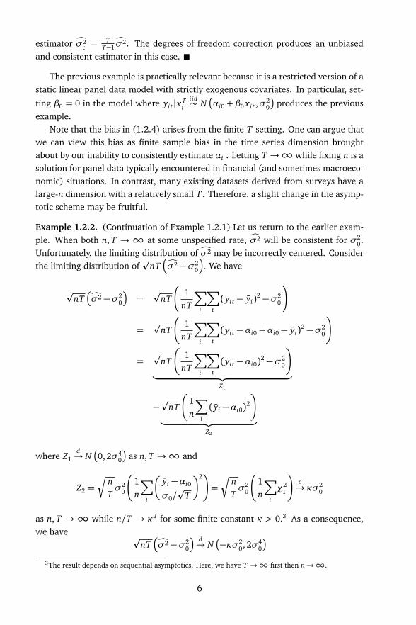
Example 1.2.2. (Continuation of Example 1.2.1) Let us return to the earlier exam-ple. When both n, T →∞ at some unspecified rate, cσ2 will be consistent for σ2

0.Unfortunately, the limiting distribution of cσ2 may be incorrectly centered. Considerthe limiting distribution of

pnT

cσ2 −σ20

. We have

pnT

cσ2 −σ20

=p

nT

1nT

∑

i

∑

t

(yi t − yi)2 −σ2

0

=p

nT

1nT

∑

i

∑

t

(yi t −αi0 +αi0 − yi)2 −σ2

0

=p

nT

1nT

∑

i

∑

t

(yi t −αi0)2 −σ2

0

︸ ︷︷ ︸

Z1

−p

nT

1n

∑

i

( yi −αi0)2

︸ ︷︷ ︸

Z2

where Z1d→ N

0, 2σ40

as n, T →∞ and

Z2 =s

nTσ2

0

1n

∑

i

yi −αi0

σ0/p

T

2

=s

nTσ2

0

1n

∑

i

χ21

p→ κσ2

0

as n, T →∞ while n/T → κ2 for some finite constant κ > 0.3 As a consequence,we have p

nT

cσ2 −σ20

d→ N

−κσ20, 2σ4

0

3The result depends on sequential asymptotics. Here, we have T →∞ first then n→∞.

6

This example shows that the relative growth rates of the two dimensions influencethe magnitude of the nonzero center −κσ2

0. This nonzero center disappears whenn/T → 0. Otherwise, we can remove the nonzero center as follows:

pnT

cσ2 −σ20

+ Z2 =p

nT

cσ2 −σ20 +

σ20

T

d→ N

0, 2σ40

.

By plugging in a consistent estimator for σ20/T under this asymptotic scheme, we are

able to bias-correct cσ2. The bias-corrected estimator cσ2c = cσ2+cσ2/T will have a lim-

iting distribution that is centered at zero. Interestingly, the asymptotic variance of cσ2c

coincides with the asymptotic variance of cσ2. Finally, note thatEcσ2c = σ

20

1− 1/T 2

.As a result, this corrected estimator is different from the degrees of freedom correc-tion considered in Example 1.2.1 because this corrected estimator is biased for fixedT but it no longer has the O

T−1

bias.

The discussion in Examples 1.2.1 and 1.2.2 provides ways in which we can achieveeither consistency for fixed T or a correctly centered asymptotic distribution whenboth n, T →∞ at rate n/T → κ2. First, we have a closed form solution (1.2.3) forthe MLE of the structural parameter and a complete specification of the density ofthe data. Thus, we can derive the finite-sample distribution of (1.2.3). Second, thebias of the MLE in (1.2.3) also has a closed form and does not depend on αi (see(1.2.4)). In general, these conditions rarely arise so a general characterization of thenonzero center is needed, as seen in the next example.

Example 1.2.3. (Hahn and Newey (2004), Arellano and Hahn (2007), and Hahnand Kuersteiner (2011)) In the previous example, we have seen an indication thatthe bias in the estimator for the parameter of interest in a model with inciden-tal parameters is of order O

T−1

. We can think of this bias as time series finitesample bias and consider again the asymptotic setting where both n, T →∞ andn/T → κ2. This asymptotic setting will allow us to more generally approximatethe asymptotic bias in the estimator and then reduce its impact. Assume that bθis a consistent estimator under this asymptotic setting, i.e. lim

T→∞θT = θ0, where

θT is the large-n, fixed-T limit of some extremum estimator. Further assume thatp

nT

bθ − θT

d→ N (0,Ω). Under these assumptions along with a stochastic expan-

sion of θT , i.e., θT = θ0 + B/T +O

T−2

, we can write

pnT

bθ − θ0

=p

nT

bθ − θT

+p

nT (θT − θ0)

=p

nT

bθ − θT

+p

nTBT+p

nTO

T−2

=p

nT

bθ − θT

+s

nT

B +Os

nT 3

d→ N (Bκ,Ω) . (1.2.5)

7

Note that (1.2.5) is not centered at 0. In the previous example, we were able to derivethat B = −σ2

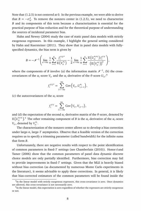
0. To remove the nonzero center in (1.2.5), we need to characterizeB and its components of this term because a characterization is essential for thepractical purpose of bias reduction and for the theoretical purpose of understandingthe sources of incidental parameter bias.

Hahn and Newey (2004) study the case of static panel data models with strictlyexogenous regressors. In this example, I highlight the general setting consideredby Hahn and Kuersteiner (2011). They show that in panel data models with fully-specified dynamics, the bias term is given by

B = −I −1

limn→∞

1n

n∑

i=1

f V Uαi

E

Vαii t

−12

limn→∞

1n

n∑

i=1

E

Uαiαii t

f V Vi

E

Vαii t

2

!

,

where the components of B involve (a) the information matrix I −1, (b) the cross-covariances of the αi-score Vi t and the αi-derivative of the θ -score Ui t :

4

f V Uαi =

∞∑

l=−∞

Cov

Vi t , Uαii,t−l

,

(c) the autocovariances of the αi-score

f V Vi =

∞∑

l=−∞

Cov

Vi t , Vi,t−l

,

and (d) the expectation of the second αi-derivative matrix of the θ -score, denoted byE

Uαiαii t

.5 The other remaining component of B is the αi-derivative of the αi-scoreVi t , denoted by Vαi

i t .The characterization of the nonzero center allows us to develop a bias correction

under large-n, large-T asymptotics. Observe that a feasible version of the correctionrequires us to specify a trimming parameter (called bandwidth) for the infinite sumsthat form B.

Unfortunately, there are negative results with respect to the point identificationof common parameters in fixed-T settings (see Chamberlain (2010)). Honoré andTamer (2006) show that the common parameters of panel data dynamic discretechoice models are only partially identified. Furthermore, bias correction may failto provide improvements in fixed-T settings. Given that the MLE is heavily biasedwithout bias correction (as documented by numerous Monte Carlo experiments inthe literature), it seems advisable to apply these corrections. In general, it is likelythat bias-corrected estimators of the common parameters will be found inside the

4In the linear model with strictly exogenous regressors, this cross-covariance is zero. Once dynamicsare allowed, this cross-covariance is not necessarily zero.

5In the linear model, this expectation is zero regardless of whether the regressors are strictly exogenousor not.

8

identified set. Although no proof of the previous claim exists, we obtain point iden-tification anyway once T becomes very large.

Observe that the examples so far apply to panel data models with strictly ex-ogenous regressors and variables with fully-specified feedback mechanisms. On theother hand, GMM based estimation of linear dynamic panel data methods in the spiritof Arellano and Bond (1991) can in principle allow for regressors whose dynamicsare not fully modeled. Unfortunately, these GMM estimators also have an asymptoticdistribution with a nonzero center under large-n, large-T asymptotics (see Alvarezand Arellano (2003)). Furthermore, these GMM estimators have been documentedto have poor finite sample performance and are susceptible to weak instruments (seeBun and Sarafidis (2015) and its references).

It should not be surprising that there is no uniformly good solution to the inci-dental parameter problem that would apply to every theoretical or empirical situa-tion. As a result, it helps to look for solutions on a case-by-case basis. One possibleapproach is to exploit the properties of the chosen parametric family to develop abias-correction. For instance, in Example 1.2.1, consider transforming the data yi t

into yi t − yi . The transformation allows us to eliminate the αi ’s because the distribu-tion of the transformed data only depends on σ2

0. As a result, the likelihood functionformed from the transformed data can be used to conduct estimation and inferencefor σ2

0. The resulting likelihood is called a marginal likelihood in the statistical lit-erature.6 Yet, it may be very difficult to find transformations or even subsets of thedata that will allow us to construct a marginal likelihood. Despite this, there are suc-cessful applications of this idea even outside the likelihood setting as the followingexample illustrates.

Example 1.2.4. (Honoré, 1992) Consider a linear panel data regression model wherey∗i t = αi + β x i t + εi t for i = 1, . . . , n and t = 1, 2. For simplicity, assume that x i t isscalar. Assume that

y∗i1, x i1, y∗i2, x i2

: i = 1, . . . , n

form a random sample but weonly get to observe data on both y and x when y∗i1 > 0 and y∗i2 > 0. Further assumethat εi1 and εi2 are independent, identically and continuously distributed conditionalon (x i1, x i2,αi) for all i.

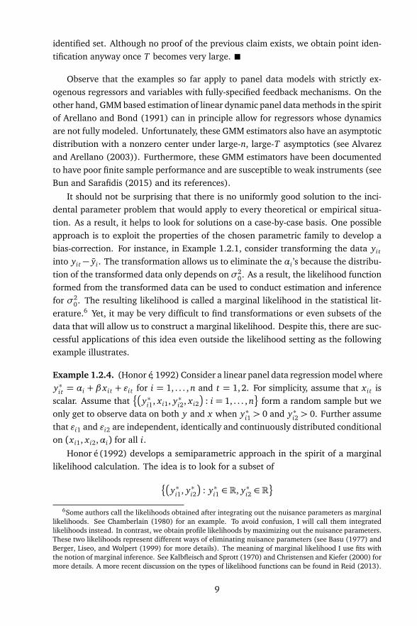
Honoré (1992) develops a semiparametric approach in the spirit of a marginallikelihood calculation. The idea is to look for a subset of

y∗i1, y∗i2

: y∗i1 ∈ R, y∗i2 ∈ R

6Some authors call the likelihoods obtained after integrating out the nuisance parameters as marginallikelihoods. See Chamberlain (1980) for an example. To avoid confusion, I will call them integratedlikelihoods instead. In contrast, we obtain profile likelihoods by maximizing out the nuisance parameters.These two likelihoods represent different ways of eliminating nuisance parameters (see Basu (1977) andBerger, Liseo, and Wolpert (1999) for more details). The meaning of marginal likelihood I use fits withthe notion of marginal inference. See Kalbfleisch and Sprott (1970) and Christensen and Kiefer (2000) formore details. A more recent discussion on the types of likelihood functions can be found in Reid (2013).

9

that is unaffected by truncation. Observe that such a subset allows us to eliminateαi by differencing. In other words, we have y∗i1 = yi1 , y∗i2 = yi2 and both timeseries observations obey yi t = αi+β x i t+εi t . Notice that this differencing strategy isexactly the same strategy applied to a linear panel data model (as in Example 1.2.1).

Define ∆yi = yi1 − yi2, ∆x i = x i1 − x i2, and ∆εi = εi1 − εi2. Assume thatβ∆x i > 0. Consider the following sets

A =

y∗i1, y∗i2

: y∗i1 > β∆x i , y∗i2 > y∗i1 − β∆x i

,

B =

y∗i1, y∗i2

: y∗i1 > β∆x i , 0< y∗i2 < y∗i1 − β∆x i

.

Notice that whenever y∗i1 > β∆x i , we must have y∗i2 > 0. Observe that

Pr

y∗i1, y∗i2

∈ A|x i1, x i2,αi

= Pr

y∗i2 − y∗i1 > −β∆x i , y∗i2 + y∗i1 > β∆x i |x i1, x i2,αi

= Pr (εi2 − εi1 > 0,εi2 + εi1 > −2αi − 2β x i2|x i1, x i2,αi)

= Pr

∆εi < 0|x i1, x i2,αi ,εi2 + εi1 > −2αi − 2β x i2︸ ︷︷ ︸

Di

×Pr (Di |x i1, x i2,αi) .

Similarly, we can write

Pr

y∗i1, y∗i2

∈ B|x i1, x i2,αi

= Pr

y∗i2 − y∗i1 < −β∆x i , y∗i2 + y∗i1 > β∆x i |x i1, x i2,αi

= Pr (εi2 − εi1 < 0,εi2 + εi1 > −2αi − 2β x i2|x i1, x i2,αi)

= Pr (∆εi > 0|x i1, x i2,αi , Di)Pr (Di |x i1, x i2,αi)

Under the assumption that the distribution of ∆εi conditional on εi1 + εi2 and on(x i1, x i2,αi) is symmetric and unimodal around zero,7 we can then conclude that

Pr

y∗i1, y∗i2

∈ A|x i1, x i2,αi

= Pr

y∗i1, y∗i2

∈ B|x i1, x i2,αi

.

Furthermore, these two sets are unaffected by truncation and will be observable(since these sets satisfy y∗i1 > β∆x i > 0 and y∗i2 > 0). As a result,

Pr ((yi1, yi2) ∈ A|x i1, x i2) = Pr ((yi1, yi2) ∈ B|x i1, x i2) .

Therefore, the union of these two sets

A∪ B = (yi1, yi2) : yi1 > β∆x i , yi2 > 0

7See Honoré (1992) for a sufficient condition.

10

is the basis for constructing a moment condition that only involves the observablesbut not the fixed effect αi . Observe further that

E [1 (yi1, yi2) ∈ A∆εi |x i1, x i2,αi]

=ˆ

1(yi1,yi2)∈Auf∆ε|x1,x2,α,D (u) du

=

ˆ 0

−∞uf∆ε|x1,x2,α,D (u) du

F∆ε|x1,x2,α,D (0)Pr (Di |x i1, x i2,αi)

=

ˆ 0

−∞uf∆ε|x1,x2,α (−u) du

1− F∆ε|x1,x2,α,D (0)

Pr (Di |x i1, x i2,αi)

=−ˆ ∞

0v f∆ε|x1,x2,α (v) dv

1− F∆ε|x1,x2,α,D (0)

Pr (Di |x i1, x i2,αi)

= −E [1 (yi1, yi2) ∈ B∆εi |x i1, x i2,αi] . (1.2.6)

The previous derivation involves the expectation of a truncated random variable andthe i.i.d. assumption on the errors. We use the symmetry assumption to obtain thethird equality. Using (1.2.6), we are able to show that the moment condition

E [1 (yi1, yi2) ∈ A∪ B (∆yi − β∆x i)∆x i]

= E [1 (yi1, yi2) ∈ A∆εi∆x i] +E [1 (yi1, yi2) ∈ B∆εi∆x i]

= E [E [1 (yi1, yi2) ∈ A∆εi∆x i |x i1, x i2,αi]]

+E [E [1 (yi1, yi2) ∈ B∆εi∆x i |x i1, x i2,αi]] (1.2.7)

= 0

is satisfied, where 1 (· ) is the indicator function. The case where β∆x i ≤ 0 is analo-gous and will be part of the criterion function for estimating β . Notice that withoutthe indicator function in (1.2.7), we have the moment condition for β in the staticlinear panel data model with strictly exogenous covariates. A least squares objectivefunction can be formed where the resulting first-order condition is exactly the sampleanalog of (1.2.7).8

Searching for a suitable subset of the data is what makes marginal likelihoodapproaches (or any other approach in the same spirit) highly model-specific. Fur-thermore, assumptions have to be changed in very specific ways to accommodateslight changes in the model. Extensions of the previous example to allow for laggeddependent variables can be found in Honoré (1993) but require a modification of the

8See Honoré (1992) for more details.

11

argument along with the assumptions in the previous example. Abrevaya (1999) pro-poses an estimator for fixed effects models with an unknown transformation of thedependent variable that also has the flavor of a marginal likelihood approach. Strictlyspeaking, the estimators discussed here are semiparametric in nature but the com-mon feature is the search for subsets of the data from which to construct momentconditions or likelihoods that do not depend on αi , but are informative about thestructural parameters. Bonhomme (2012) provides a theory that allows any user ofa likelihood-based panel data model with strictly exogenous regressors to constructmoment conditions that are free of the fixed effects. One can think of the theory as ageneral treatment of the marginal likelihood approach. Unfortunately, it is possiblethat certain panel models will not possess moment conditions that are informative ofthe structural parameters. Aspects of this theory will be discussed further in Example1.2.7.

Yet another approach is to find appropriate conditioning sets so that a conditionallikelihood that does not depend on αi can be constructed. As a result, the score of theconditional likelihood is itself a moment condition that is free of αi . The followingexample illustrates this approach in a dynamic logit model.

Example 1.2.5. (Chamberlain, 1985; Maddala, 1987; Honoré and Kyriazidou, 2000)Consider a dynamic panel logit model with one strictly exogenous regressor. In par-ticular, we have for i = 1, . . . , n and t = 1, . . . , T :

Pr

yi t = 1|x i1, . . . , x iT , yi0, . . . , yi,T−1,αi

=exp

β x i t + γyi,t−1 +αi

1+ exp

β x i t + γyi,t−1 +αi

. (1.2.8)

This means that

Pr

yi t = 0|x i1, . . . , x iT , yi0, . . . , yi,T−1,αi

=1

1+ exp

β x i t + γyi,t−1 +αi

.

Assume that yi0 is observed and T = 3. Hence, we have a total of four observations.Define the sets

A = yi1 = 0, yi2 = 1, yi3 = d3 ,

B = yi1 = 1, yi2 = 0, yi3 = d3 ,

where d3 ∈ 0, 1. Let xi = (x i1, x i2, x i3) and d0 ∈ 0, 1. We can calculate thefollowing conditional probabilities:

Pr (A|xi , yi0 = d0,αi)

= Pr (yi3 = d3|xi , yi0 = d0, yi1 = 0, yi2 = 1)

×Pr (yi2 = 1|xi , yi0 = d0, yi1 = 0)× Pr (yi1 = 0|xi , yi0 = d0)

12

=exp (d3 (β x i3 + γ+αi))1+ exp (β x i3 + γ+αi)

×exp (β x i2 +αi)

1+ exp (β x i2 +αi)

×1

1+ exp (β x i1 + γd0 +αi),

Pr (B|xi , yi0 = d0,αi)

= Pr (yi3 = d3|xi , yi0 = d0, yi1 = 1, yi2 = 0)

×Pr (yi2 = 0|xi , yi0 = d0, yi1 = 1)× Pr (yi1 = 1|xi , yi0 = d0)

=exp (d3 (β x i3 +αi))1+ exp (β x i3 +αi)

×1

1+ exp (β x i2 + γ+αi)

×exp (β x i1 + γd0 +αi)

1+ exp (β x i1 + γd0 +αi).

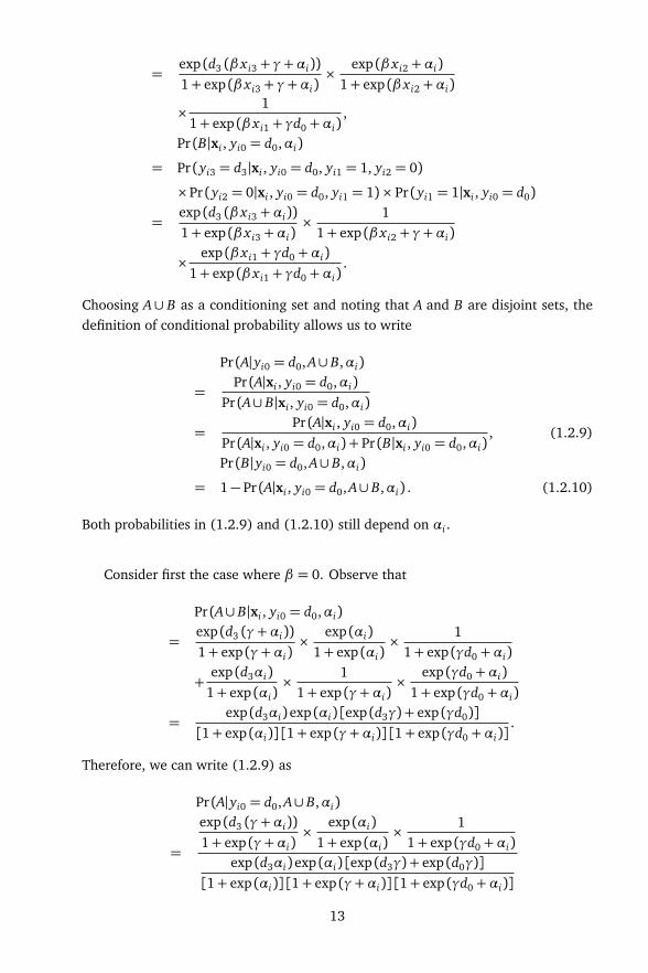
Choosing A∪ B as a conditioning set and noting that A and B are disjoint sets, thedefinition of conditional probability allows us to write

Pr (A|yi0 = d0, A∪ B,αi)

=Pr (A|xi , yi0 = d0,αi)

Pr (A∪ B|xi , yi0 = d0,αi)

=Pr (A|xi , yi0 = d0,αi)

Pr (A|xi , yi0 = d0,αi) + Pr (B|xi , yi0 = d0,αi), (1.2.9)

Pr (B|yi0 = d0, A∪ B,αi)

= 1− Pr (A|xi , yi0 = d0, A∪ B,αi) . (1.2.10)

Both probabilities in (1.2.9) and (1.2.10) still depend on αi .

Consider first the case where β = 0. Observe that

Pr (A∪ B|xi , yi0 = d0,αi)

=exp (d3 (γ+αi))1+ exp (γ+αi)

×exp (αi)

1+ exp (αi)×

11+ exp (γd0 +αi)

+exp (d3αi)

1+ exp (αi)×

11+ exp (γ+αi)

×exp (γd0 +αi)

1+ exp (γd0 +αi)

=exp (d3αi)exp (αi) [exp (d3γ) + exp (γd0)]

[1+ exp (αi)] [1+ exp (γ+αi)] [1+ exp (γd0 +αi)].

Therefore, we can write (1.2.9) as

Pr (A|yi0 = d0, A∪ B,αi)

=

exp (d3 (γ+αi))1+ exp (γ+αi)

×exp (αi)

1+ exp (αi)×

11+ exp (γd0 +αi)

exp (d3αi)exp (αi) [exp (d3γ) + exp (d0γ)][1+ exp (αi)] [1+ exp (γ+αi)] [1+ exp (γd0 +αi)]

13

=exp (d3γ)

exp (d3γ) + exp (d0γ).

Similarly, (1.2.10) can be written as

Pr (B|yi0 = d0, A∪ B,αi) =exp (d0γ)

exp (d3γ) + exp (d0γ).

Both these conditional probabilities do not depend on αi and can be used to form aconditional likelihood depending only on γ.

Now, consider the case where β 6= 0. Honoré and Kyriazidou (2000) show that byfurther conditioning on the event x i2 = x i3, assumed to have positive probability,we can eliminate the dependence of (1.2.9) and (1.2.10) on αi . In particular, wehave

Pr (A|xi , yi0 = d0, A∪ B, x i2 = x i3,αi) =1

1+ exp (β (x i1 − x i2) + γ (d0 − d3)),

Pr (B|xi , yi0 = d0, A∪ B, x i2 = x i3,αi) =exp (β (x i1 − x i2) + γ (d0 − d3))

1+ exp (β (x i1 − x i2) + γ (d0 − d3))

and a conditional likelihood will be formed from observations where x i2 = x i3 andyi1 + yi2 = 1, i.e., a conditional MLE can be computed from the following optimiza-tion problem:

maxβ ,γ

N∑

i=1

1 yi1 + yi2 = 11 x i2 = x i3 log

[exp (β (x i1 − x i2) + γ (d0 − d3))]yi1

1+ exp (β (x i1 − x i2) + γ (d0 − d3))

.

The condition x i2 = x i3 is unlikely to be satisfied, so a kernel function replaces theindicator function above. Because we introduce a kernel function, the estimatorsfor the structural parameters converge at a rate slower than the usual parametricrate. We also cannot allow for time dummies because they never satisfy x i2 = x i3 bydefinition. Extensions to a semiparametric specification of the probability function(1.2.8) in the spirit of Manski (1987b), the multinomial logit case, and more thanfour observations for every i are available in Honoré and Kyriazidou (2000).

Even though the approaches in Examples 1.2.4 and 1.2.5 are both appealing andinsightful, the search for appropriate transformations of the data or appropriate con-ditioning sets will become cumbersome when T is a bit larger or when we makeslight changes to the model.

Some authors like Wooldridge (2005b) and Arellano and Bonhomme (2011) ar-gue that the structural parameters may not be of primary interest especially for policy.Policy parameters are usually of the form E

m

x Ti ,αi

, where m is some functionof the regressors and unobserved heterogeneity. These policy parameters have beencalled many names depending on the form of m, such as the average structural func-

14

tion (Blundell and Powell, 2004), quantile structural function (Chernozhukov et al.,2013), average index function (Lewbel, Dong, and Yang, 2012), average marginaleffect (Wooldridge, 2005b), and local average response (Altonji and Matzkin, 2005).These policy parameters represent summary measures that describe outcomes of cer-tain thought experiments. One such thought experiment involves a prediction ofwhat m will be when we set x T

i at some fixed value x while holding unobservedheterogeneity constant. Another thought experiment would involve predictions asto how m changes when we change the value x while holding unobserved hetero-geneity constant. Unfortunately, these policy parameters are hard to identify andrequire understanding the tradeoffs among competing assumptions as seen in thenext example.

Example 1.2.6. (Hoderlein and White (2012)) Consider the following nonseparablemodel where Yi t = g (X i t ,αi ,εi t) for i = 1, . . . , n and t = 1,2. An object of interest forpolicy is how E (Yi t |X i1 = x1, X i2 = x2) changes with x1 or x2, holding the source ofunobserved heterogeneity constant. In other words, the policy parameters of interestor average marginal effects at x1 and x2, are given by

M E1 (x1, x2) =ˆ ˆ

∂ g (x1, a, e)∂ x1

fαi ,εi1|X i(a, e|x1, x2) da de,

M E2 (x1, x2) =ˆ ˆ

∂ g (x2, a, e)∂ x2

fαi ,εi2|X i(a, e|x1, x2) da de.

Had we known what fαi ,εi t |X iis, then everything becomes straightforward and calcu-

lating M E1 (x) and M E2 (x) can be done directly. This situation is really the ideabehind the calculation of average marginal effects from fully parametric modelswith correlated random effects proposed by Chamberlain (1984) and Wooldridge(2005b). If we do not know fαi ,εi t |X i

, we have to indirectly recover M E1 (x) andM E2 (x) somehow. In particular, we have the following

E (Yi1|X i1 = x1, X i2 = x2) =ˆ ˆ

g (x1, a, e) fαi ,εi1|X i(a, e|x) da de,

E (Yi2|X i1 = x1, X i2 = x2) =ˆ ˆ

g (x2, a, e) fαi ,εi2|X i(a, e|x) da de,

with four derivatives given by

∂E (Yi1|X i1 = x1, X i2 = x2)∂ x1

= M E1 (x1, x2)

+ˆ ˆ

g (x1, a, e)∂ fαi ,εi1|X i

(a, e|x)∂ x1

da de

∂E (Yi1|X i1 = x1, X i2 = x2)∂ x2

=ˆ ˆ

g (x1,α,ε)∂ fαi ,εi1|X i

(a, e|x)∂ x2

da de

15

∂E (Yi2|X i1 = x1, X i2 = x2)∂ x1

=ˆ ˆ

g (x2, a, e)∂ fαi ,εi2|X i

(a, e|x)∂ x1

da de

∂E (Yi2|X i1 = x1, X i2 = x2)∂ x2

= M E2 (x1, x2)

+ˆ ˆ

g (x2, a, e)∂ fαi ,εi2|X i

(a, e|x)∂ x2

da de

The left hand side of the above derivatives are observable from the data. In con-trast, the right hand side involves objects that are unknown to the econometrician,specifically the distribution of the errors fαi ,εi t |X i

and their associated derivatives∂ fαi ,εi t |X i

/∂ x . To recover M E1 (x1, x2) and M E2 (x1, x2) from the four precedingequations, we have to make further assumptions since there are more unknownsthan the number of equations. It is not enough that we assume a form of time homo-geneity (which ensures that a repeated measurement will be beneficial with respectto controlling for αi), i.e.

fαi ,εi1|X i= fαi ,εi2|X i

because we are still unable to completely remove the distortion caused by the effect ofchanging x1 or x2 on the distribution of the errors. In addition, we have to conditionon the set where X i1 = X i2 = x to completely remove this distortion. As a result, weare able to identify the marginal effects by conditioning on an appropriate set underno assumptions about the nonseparable model and the distribution of the errors(aside from time homogeneity):9

M E1 (x) =∂E (Yi1|X i1 = X i2 = x)

∂ x1−∂E (Yi2|X i1 = X i2 = x)

∂ x1,

M E2 (x) =∂E (Yi2|X i1 = X i2 = x)

∂ x2−∂E (Yi1|X i1 = X i2 = x)

∂ x2.

Without conditioning on X i1 = X i2 = x , there are multiple avenues to recover the av-erage marginal effect. In general, we can only partially identify the average marginaleffect when there are bounds on g (X i t ,αi ,εi t) (see Chernozhukov et al. (2013)).

To avoid conditioning on X i1 = X i2 = x , we may consider correlated randomeffects strategies that use exchangeability (see Altonji and Matzkin (2005) for more)and dimension reduction to construct "instruments" that allow us to nullify the dis-tortions brought about by the effect of changing x on the distribution of the errors.Bester and Hansen (2009b) show that if there exists a sufficient statistic that could re-duce the dimension of the conditioning set X i1 = x1, X i2 = x2, . . . , X iT = xT , thenit is possible to recover the average marginal effect if T ≥ 3. Bester and Hansen(2009b) are actually able to weaken the assumption of time homogeneity in this

9Imposing further restrictions may help in trading off some assumptions for others. The gains will haveto be explored on a case-by-case basis.

16

case. Testing some of these assumptions is the subject of Ghanem (2015).Note that the discussion so far focuses on strictly exogenous regressors. Extend-

ing the ideas to dynamic models are not very straightforward under the conditionsmaintained in the earlier discussion. Bounds for the dynamic model are also avail-able in Chernozhukov et al. (2013). Parametric approaches that fully specify thedistribution of the errors are available in Wooldridge (2005b). Large-T bias correc-tions of marginal effects obtained from parametric fixed-effects models can be foundin Hahn and Newey (2004), Bester and Hansen (2009a), and Fernandez-Val (2009).

In the final example, I show that reducing the support of the distribution of thefixed effects may be helpful in identification of structural parameters. The lack ofpoint identification of structural parameters in nonlinear panel data models has beendocumented by Honoré and Tamer (2006) and Chamberlain (2010) if we leave thedistribution of the fixed effects unspecified. This lack of point identification can alsobe illustrated in the next example.

Example 1.2.7. (Bajari et al. (2011) and Bonhomme (2012)) Consider the followingpanel binary choice model with strictly exogenous regressors x i t :

Pr (yi t = 1|x i ,αi) = H (αi + β x i t) , i = 1, . . . , n; t = 1, . . . , T (1.2.11)

where the distribution of the individual-specific fixed effectαi given x i = (x i1, . . . , x iT )has finite and discrete support, i.e.

Pr (αi = αk|x i = x) = πx ,k, k = 1, . . . , K .

A fixed-effects setup means that we leave the πx ,k ’s unspecified and possibly depen-dent on x . Assume further that the inverse link function H is specified in advance.Since the αi ’s are unobservable, we have to look at the full conditional distributionof yi = (yi1, . . . , yiT ) given x i = x alone. As a consequence of the law of total prob-ability, this full conditional distribution can be written as

Pr (yi = y|x i = x) =K∑

k=1

Pr (yi = y|x i = x ,αi = αk;β)Pr (αi = αk|x i = x) (1.2.12)

for some binary sequence y . The left hand side of (1.2.12) can be recovered fromthe data on frequencies of each of the 2T possible binary sequences. We can collectevery (1.2.12) for each possible binary sequence so that we have a matrix equation

Py|x = Px (β)πx ,

where πx =

πx ,1, . . . ,πx ,K

Tis a K×1 vector, Px (β) is a 2T ×K matrix based on the

17

specification (1.2.11), and Py|x is a 2T×1 vector of conditional probabilities observedfrom the data.

Instead of differencing out every αi which is not generalizable outside linearmodels, we difference out πx by annihilating the matrix Px (β), i.e.

I − Px (β) Px (β)− Py|x =

I − Px (β) Px (β)− Px (β)πx = 0. (1.2.13)

Note that Px (β)− is the Moore-Penrose inverse of Px (β). The main message behind

(1.2.13) is not that it is possible to construct moment conditions that do not dependon αi but that the rank of the matrix Px (β) matters. If we know that K ≥ 2T , then(1.2.13) is not informative of β at all. On the other hand, considering models for thefixed effects for which K < 2T may be useful. We can interpret K < 2T as the supportof the fixed effects being less rich than the support of outcomes. In general, we willnot know whether K < 2T or otherwise. There are empirical situations, such as thegame-theoretic model estimated by Hahn and Moon (2010) and the one discussedin Chapter 3, where we would know the value of K .

In Hahn and Moon (2010), the reduced support of the fixed effects arises becausethe fixed effects represent which of the two pure strategy equilibria is selected byplayers and maintained over time. Further work that allow for time-varying fixedeffects with limited support has been studied by Bonhomme and Manresa (2015).The latter paper and Hahn and Moon (2010) have shown that bias correction in alarge-n, large-T context like we have seen in Example 1.2.3 is not needed at all.

1.3 How should we respond?

The discussion in the previous section comes from a perspective which emphasizeseither the elimination of nuisance parameters or the robustification of estimationand inference methods in the presence of nuisance parameters. Furthermore, thedistribution of the fixed effects is left unspecified as seen in Examples 1.2.1 to 1.2.5.As models become more complicated, this emphasis may become increasingly un-tenable, especially when there is meaning to be attached to nuisance parameters orwhen interest centers on functions of interest and nuisance parameters as seen in Ex-amples 1.2.6 and 1.2.7. Empirically relevant models also have to allow for dynamicsand predetermined regressors. Therefore, we need to search for methods that workin slightly complicated settings at the cost of making assumptions that may never-theless be motivated theoretically or empirically. I now describe the ideas pursuedin the succeeding chapters.

Many empirical situations (see Chapter 2 for examples) call for the estimationof a dynamic binary choice model with fixed effects. In Chapter 2, I demonstratethat it is inappropriate to estimate such a model by applying IV to a dynamic linearprobability model. Motivations behind the use of a dynamic linear probability model

18

include the ability to directly recover average marginal effects and the availabilityof software without additional programming. IV or GMM based estimators of thedynamic linear probability model can also allow for predetermined regressors. Wesaw the difficulties in recovering average marginal effects and allowing for dynamicsin Example 1.2.6. The main results of the chapter actually suggest that IV estimatorsof the linear probability model converge to an average marginal effect with incorrectweighting. Furthermore, this large-n limit might not even be found inside the large-n limit of the bounds proposed by Chernozhukov et al. (2013). In addition, these IVestimators do not converge to the true average marginal effect even as T →∞. As aresult, this chapter gives an example for which dealing with the incidental parameterproblem using IV may not be a good response.

Another empirical situation of interest involves the estimation of simultaneouslydetermined discrete outcomes. Allowing for fixed effects in these models has notbeen explored fully, since most research has focused on either cross-sectional models,continuous outcomes, or random effects (see for example, the research by Cornwell,Schmidt, and Wyhowski (1992), Leon-Gonzalez (2003), Matzkin (2008), Matzkin(2012), and Masten (2015)). Parameter identification in these models is furthercomplicated by the nonexistence of a unique reduced form. One way of partiallyresolving the identification problem is to introduce coherency conditions. Unfortu-nately, the coherency condition needs to be imposed a priori. In Chapter 3, I proposeusing panel data to estimate such models by allowing the data to determine how thecoherency condition will hold. The manner in which the coherency condition holdscan be represented as an incidental parameter that has finite support, in the spirit ofwhat we have seen in Example 1.2.7.

The discussion in Example 1.2.3 is an estimator-based bias correction. One willobserve that papers proposing an analytical correction of the estimator typically mo-tivate the correction using the score. In Chapter 4, I develop a score-based correc-tion involving projections. This approach is a useful and intuitive alternative whenconstructing estimating equations for the structural parameters that are relativelyinsensitive to inconsistent plug-ins. I show that the method can produce familiarestimators in special cases. I also show that projection exploits correct specificationto reap the gains from bias reduction especially when T is very small.

Although the notion of time-invariant heterogeneity is hardly unique, a large gapexists between specifications where we allow for full heterogeneity (i.e., acknowl-edging that all units are different from each other) and full homogeneity (i.e., ac-knowledging that all units are the same). This gap enables us to explore differentnotions of partial pooling. Researchers acknowledge that units might be differentfrom one another yet they may believe that some units are more alike than others.Despite this, they might be unwilling to specify which units are different from eachother and which units are similar to one another. I formalize the preceding intuitionby allowing some incidental parameters to take on the same value, namely zero.

19

In Chapter 5, I demonstrate that some notion of sparsity of the incidental parame-ters may be useful in constructing fixed-T consistent estimators that converge at theroot-n rate. In particular, I tune the lasso (see Tibshirani (1996; 2011) and Chapter5 for more) so that it will be able to detect the non-zero incidental parameters. Asubsample for which the incidental parameters are set to zero can then be used forestimation and inference. This is in contrast to the machine learning and big dataliterature where the main developments have concentrated on uncovering non-zeroeffects in a sea of zero effects.

The four essays included in this thesis demonstrate several different ways to copewith the incidental parameter problem. None of these essays offer a general solution.Instead, these essays provide situations for which the incidental parameter problemmay not be a serious impediment to theoretical and empirical work. However, Irestrict myself to parametric situations and leave the nonparametric situations tofuture research.

20

Chapter 2

On IV estimation of a dynamiclinear probability model withfixed effects

2.1 Introduction

Many researchers still use the dynamic linear probability model (LPM) with fixed ef-fects when analyzing a panel of binary choices. Several applications of the dynamicLPM with fixed effects can be found in papers published in top journals. Applicationsinclude assessing the magnitude of state dependence in female labor force participa-tion (Hyslop, 1999), examining the factors that affect exporting decisions (Bernardand Jensen, 2004), determining the effect of income on transitions in and out ofdemocracy (Acemoglu et al., 2009), and determining how overnight rates affect abank’s decision to provide loans (Jiménez et al., 2014). A more suitable approach,however, is to use limited dependent variable (LDV) models when analyzing discretechoice. Unfortunately, the inclusion of fixed effects creates an incidental parameterproblem that complicates the estimation of average marginal effects, especially whenthe time dimension is small (see the survey by Arellano and Bonhomme (2011)).Resorting to a random effects or correlated random effects approach may requirespecifying the full distribution of the fixed effects and initial conditions1 – some-thing that researchers may be unwilling to do because of the lack of specific subject

1Typically, only the first two moments of the full distribution are required in the case of linear models.In contrast, nonlinear models would typically require the full distribution because we use this distributionto integrate the fixed effects out of the distribution. There are some approaches that can be thought of asbeing in the middle of correlated random effects approaches and fixed-effects approaches. A prominentexample is using a special regressor to consistently estimate common parameters without imposing aparametric assumption on the distribution of the fixed effects and initial conditions, as proposed by Honoréand Lewbel (2002).

21

matter knowledge to construct such a distribution. Linear dynamic panel data meth-ods present an alternative that allows for fixed effects, dynamics, predeterminedregressors, fewer functional form restrictions, and even allow for heteroscedasticity.Therefore, using methods intended for linear dynamic panel data models seems tobe an attractive alternative in this setting.

In contrast, my results provide arguments against a commonly held sentimentamong researchers expressed quite forcefully in Angrist and Pischke (2009, p.107):

The upshot of this discussion is that while a nonlinear model may fit the CEF for LDVsmore closely than a linear model, when it comes to marginal effects, this probably mattersa little. This optimistic conclusion is not a theorem, but, as in the empirical example here,it seems to be fairly robustly true.

Why, then, should we bother with nonlinear models and marginal effects? One answeris that the marginal effects are easy enough to compute now that they are automated inpackages like Stata. But there are a number of decisions to make along the way (e.g.,the weighting scheme, derivatives versus finite differences), while OLS is standardized.Nonlinear life also gets considerably more complicated when we work with instrumentalvariables and panel data. Finally, extra complexity comes into the inference step as well,since we need standard errors for marginal effects.

In this paper, I explain why usual dynamic panel data methods, specifically instru-mental variable (IV) estimation, are inappropriate for estimating average marginaleffects if the conditional expectation function (CEF) is truly nonlinear. In particular,I show the large-n limit of the Anderson-Hsiao (1981; 1982) IV estimator (hence-forth AH) is an average marginal effect but subject to incorrect weighting. Giventhat the AH estimator is a special case of GMM, estimators in the spirit of Arellanoand Bond (1991) may be subject to the same problem. I also show that the effectof this incorrect weighting does not disappear even when T is large. Furthermore,I give examples to show that there are certain parameter configurations and fixedeffect distributions for which the large-n limit of the AH estimator is outside thenonparametric bounds derived by Chernozhukov et al. (2013).

Much research has been done on whether using the LPM is suitable. A particularlyeye-catching example was provided by Lewbel, Dong, and Yang (2012). They show,in a toy example, that OLS applied to the LPM cannot even get the correct sign of thetreatment effect even in the situation where there is just a binary exogenous regressorand a high signal-to-noise ratio. Horrace and Oaxaca (2006) show that the linearpredictor for the probability of success should be in [0,1] for all observations forthe OLS estimator to be consistent for the regression coefficients because the zeroconditional mean assumption does not hold when there are observations (whether inthe sample or in the population) that produce success probabilities outside [0, 1]. Onthe other hand, Wooldridge (2010) argues that "the case for the LPM is even strongerif most the regressors are discrete and take on only a few values". Problem 15.1 ofhis book asks the reader to show that we need not worry about success probabilitiesbeing outside [0, 1] in a saturated model. If we specialize the results in Wooldridge

22

(2005a) and Murtazashvili and Wooldridge (2008) to the LPM, then they show thatfixed-effects estimation applied to the LPM with strictly exogenous regressors canbe used to consistently estimate average marginal effects under a specific correlatedrandom coefficients condition.

I organize the rest of the chapter as follows. In Section 2.2, I present an exampleto show that it is possible to use the LPM to recover an average treatment effect undervery special assumptions that researchers are unwilling to make. In Section 2.3, Iderive analytically the consequences of not meeting these special assumptions wheninterest centers on the average marginal effect of state dependence for the cases ofT = 3 and T →∞. Next, I examine the practical implications of these results using anumerical example and an empirical application on female labor force participationand fertility in Section 2.4. The last section contains concluding remarks followedby a technical appendix.

2.2 A situation where the LPM is a good idea

Suppose we have a two-period panel binary choice model with a strictly exogenousbinary regressor:

Pr (yi t = 1|x i ,αi) = Pr (yi t = 1|x i t ,αi) = H (αi + β x i t) , (2.2.1)

where H : [0,1]→ R is some inverse link function that is increasing, yi t ∈ 0, 1 andx i = (x i1, x i2) = (0,1) for all i = 1, . . . , n and t = 1, 2. Assume that for all i, we haveyi1⊥yi2|x i ,αi .

The regressor x is a strictly exogenous treatment indicator such that all individ-uals are treated in the second period but not in the first period. In other words,specification (2.2.1) is basically a before-and-after analysis. In this setting, αi is anindividual-specific fixed effect drawn from some unspecified density g (α).

Suppose one ignores the binary nature of the outcome variable yi t and one startswith an LPM with fixed effects, i.e., yi t = αi+β x i t+εi t instead. The within estimatorfor β , which is equivalent to the first-difference estimator for T = 2, is then given by

bβ =

1n

n∑

i=1

(yi2 − yi1) (x i2 − x i1)

1n

n∑

i=1

(x i2 − x i1)2

=1n

n∑

i=1

(yi2 − yi1)1 (yi1 + yi2 = 1) =1n(n01 − n10) ,

where 1 (·) is the indicator function. The second equality follows from the defini-tion of x and the implication that yi2 − yi1 = 0 for all i such that yi1 = yi2. Thethird equality follows from defining nab =

∑ni=1 1 (yi1 = a, yi2 = b) as the number

23

of observations for which we observe the sequence ab. Thus, only those i for whichyi1 6= yi2 enter into the calculation of bβ .

When we calculate the large-n limit of the within estimator, we have

bβp→ˆ

Pr (yi2 = 1|x i ,α)Pr (yi1 = 0|x i ,α) g (α) dα

−ˆ

Pr (yi2 = 0|x i ,α)Pr (yi1 = 1|x i ,α) g (α) dα

=ˆ[(1−H (α))H (α+ β)−H (α) (1−H (α+ β))] g (α) dα

=ˆ[H (α+ β)−H (α)] g (α) dα

In the situation I have described, the average marginal effect∆= E [yi2 − yi1|x i = (0, 1)]can be written as:

∆ = E [E (yi2|x i = (0,1) ,α)−E (yi1|x i = (0, 1) ,α)]

= E [E (yi2|x i2 = 1,α)−E (yi1|x i1 = 0,α)] (2.2.2)

= E [H (α+ β)−H (α)] (2.2.3)

Despite the inability of the within estimator to consistently estimate β ,2 the withinestimator does coincide with ∆ even if the true model is nonlinear. In addition, thesample analog of ∆ is exactly the within estimator.

Notice that the result arises because of a lucky coincidence of factors – (a) thestrict exogeneity of x (allowing us to obtain (2.2.2)), (b) the independence of αi

and x i (allowing us to obtain (2.2.3)), and (c) the time homogeneity assumptionbecause H does not depend on time (which follows from (2.2.1)). Despite startingfrom a fixed effects treatment of αi , one has no choice but to assume independenceof αi and x i in order to obtain (2.2.3). This already violates the need to allow forarbitrary correlation between αi and x i . It is as if an omniscient Nature did not usethe knowledge of αi to assign a corresponding treatment vector x i to every unit.

Hahn’s (2001) discussion of Angrist (2001) has already pointed out the specialconditions under which the within estimator is able to estimate an average treatmenteffect. In addition, he emphasizes that the simple strategies suggested by Angrist(2001) require knowledge of the "structure of treatment assignment and careful re-expression of the new target parameter". Chernozhukov et al. (2013) also make thesame point and further show that the within estimator converges to some weightedaverage of individual difference of means for a specific subset of the data. They alsoshow that this weighted average is not the average marginal effect of interest.

2Incidentally, Chamberlain (2010) shows that β is not even point identified in this example unless His logistic. The result of Manski (1987a) does not apply here. He shows that β is identified up to scalewhen one of the strictly exogenous regressors has unbounded support.

24

Despite all these concerns, researchers still insist on estimating LPMs with fixedeffects. One may argue that the example above does not really arise in empiricalapplications but the example already gives an indication that complicated binarychoice models estimated through an LPM are unlikely to produce intended results.In particular, the lucky coincidence of factors mentioned earlier does not hold at allfor the dynamic LPM which I discuss next.

2.3 Main results

2.3.1 The case of three time periods

Consider the following specification of a dynamic discrete choice model with fixedeffects and no additional regressors:

Pr

yi t = 1|y t−1i ,αi

= Pr

yi t = 1|yi,t−1,αi , yi0

= H

αi +ρ yi,t−1

, i = 1, . . . , n, t = 1, 2,3, (2.3.1)

where y t−1i is the past history of y , αi is an individual-specific fixed effect, yi0 is an

observable initial condition, and H : R→ [0, 1] is some inverse link function. Assumethat (yi0, yi1, yi2, yi3,αi) are independently drawn from their joint distribution forall i. I leave the joint density of (αi , yi0), denoted by f , unspecified. This datagenerating process satisfies Assumptions 1, 3, 5, and 6 of Chernozhukov et al. (2013).

If H is the logistic function, thenρ can be estimated consistently using conditionallogit (Chamberlain, 1985). If H happens to be the standard normal cdf, then ρ isnot even point-identified (Honoré and Tamer, 2006).3 In both these cases, we alsocannot point-identify the average marginal effect ∆:

∆=ˆ

Pr

yi t = 1|yi,t−1 = 1,α, y0

− Pr

yi t = 1|yi,t−1 = 0,α, y0

f (α, y0) dαd y0

(2.3.2)even if we know H but leave the density of (yi0,αi) unspecified. This averagemarginal effect is of practical interest because it measures the effect of state de-pendence in the presence of individual-specific unobserved heterogeneity.

Despite these negative results, researchers still insist on using a dynamic LPMon the grounds that linearity still provides a good approximation even if the trueH is nonlinear.4 I use this as a starting point and determine the large-n limit of IVestimators for the dynamic LPM. The linear model researchers have in mind can beexpressed as:

yi t = αi +ρ yi,t−1 + εi t , i = 1, . . . , n, t = 1, 2,3,

3Honoré and Tamer (2006) actually show that the sign of ρ is identified for any strictly increasing cdfH and unrestricted distribution of (yi0,αi).

4The dynamic LPM is really a special case of (2.3.1), where H is the identity function.

25

where εi t = yi t − E

yi t |y t−1i ,αi

. We now take first-differences to eliminate αi:

∆yi t = ρ∆yi,t−1 +∆εi t , i = 1, . . . , n, t = 2,3.

Because the differenced regressor ∆yi,t−1 is correlated with the differenced error∆εi t , IV or GMM estimators have been used to estimate ρ. Using lagged differencesas instruments, the AH estimator can be written as

bρAHd =

∑ni=1∆yi1∆yi3

∑ni=1∆yi1∆yi2

.

Because of the binary nature of the sequences (yi0, yi1, yi2, yi3) : i = 1, . . . , n, it iscertainly possible for some of the first differences to be equal to zero. Therefore,there are only certain types of sequences that enter into the expression above. If weenumerate all these 16 possible sequences, we can rewrite the estimator as

bρAHd =n0110 + n1001 − n1010 − n0101

n0100 + n1010 + n0101 + n1011,

where nabcd =∑n

i=1 1 (yi0 = a, yi1 = b, yi2 = c, yi3 = d) denotes the number of ob-servations in the data for which we observe the sequence abcd.5

It can be shown6 that the large-n limit of bρAHd is

bρAHdp→

ˆH (α) (1−H (α+ρ)) (H (α+ρ)−H (α)) g (α) dα

ˆH (α) (1−H (α+ρ)) g (α) dα

(2.3.3)

=ˆ

wd (α,ρ) (H (α+ρ)−H (α)) dα

=ˆ ˆ

wd (α,ρ)

Pr

yi t = 1|yi,t−1 = 1,α, y0

− Pr

yi t = 1|yi,t−1 = 0,α, y0

dα d y0

where

wd (α,ρ) =H (α) (1−H (α+ρ)) g (α)ˆH (α) (1−H (α+ρ)) g (α) dα

.

Note that the weighting function wd (α,ρ) depends on the true value of ρ and the

5Note that we cannot just drop those sequences for which yi1+ yi2 6= 1, like in conditional logit. If wedo this, the resulting AH estimator becomes

eρAHd =−n1010 − n0101

n0100 + n1010 + n0101 + n1011,

which is always negative regardless of the sign of ρ or ∆. Observe that identification arguments basedon the conditional logit do not necessarily translate to other inverse link functions, including that of theidentity function.

6A part of the derivation can be found in the appendix.

26

marginal distribution of the fixed effects g (α). The correct weighting function shouldhave been the joint density of (y0,α) as in (2.3.2). Therefore, bρAHd is inconsistentfor ∆ because of the incorrect weighting of the individual marginal dynamic effectH (α+ρ)−H (α).

It is difficult to give a general indication of whether we overestimate or underes-timate∆, because the results depend on the joint distribution of (y0,α). If it happensthat ρ = 0 (so that ∆= 0), then bρAHd is consistent for ∆.

The analysis above can be extended to the AH estimator which uses levels as theinstrument set. It can be shown that this AH estimator has the following form:

bρAHl =

∑ni=1

∑3t=2 yi,t−2∆yi t

∑ni=1

∑3t=2 yi,t−2∆yi,t−1

=n0110 − n0101 + n1110 − n1010 + n1100 − n1011

n1010 + n1000 + n1001 + n1011 + n0100 + n1100 + n0101 + n1101.

Calculations similar to (2.3.3) allow us to derive the large-n limit of bρAHl , i.e.

bρAHlp→

ˆ(1−H (α+ρ)) (1+H (α+ρ)) (H (α+ρ)−H (α)) f (α, 1) dα

ˆ[(1−H (α+ρ)) (1+H (α+ρ)) f (α, 1) + (1−H (α+ρ))H (α) f (α, 0)] dα

+

ˆ(1−H (α+ρ))H (α) (H (α+ρ)−H (α)) f (α, 0) dα

ˆ[(1−H (α+ρ)) (1+H (α+ρ)) f (α, 1) + (1−H (α+ρ))H (α) f (α, 0)] dα

=ˆ ˆ

wl (α,ρ, y0) (H (α+ρ)−H (α)) d y0dα

=ˆ ˆ

wl (α,ρ, y0)

Pr

yi t = 1|yi,t−1 = 1,α, y0

− Pr

yi t = 1|yi,t−1 = 0,α, y0

dα d y0,

where

wl (α,ρ, 0) =(1−H (α+ρ))H (α) f (α, 0)ˆ

[(1−H (α+ρ)) (1+H (α+ρ)) f (α, 1) + (1−H (α+ρ))H (α) f (α, 0)] dα,

wl (α,ρ, 1) =(1−H (α+ρ)) (1+H (α+ρ)) f (α, 1)ˆ

[(1−H (α+ρ)) (1+H (α+ρ)) f (α, 1) + (1−H (α+ρ))H (α) f (α, 0)] dα,

I denote f (α, 0) = Pr (y0 = 0|α) g (α) and f (α, 1) = Pr (y0 = 1|α) g (α). Note thatthe weighting function wl (α,ρ, y0) depends on the true value of ρ and the joint dis-tribution of (y0,α). Once again, we have an incorrect weighting function wl (α,ρ, y0)instead of the joint distribution of (y0,α). As a result, bρAHl is inconsistent for ∆.7

7For the case where we have one less time period, i.e. we observe sequences of the form(yi0, yi1, yi2) : i = 1, . . . , n, the large-n limit of bρAHl depends only on f (α, 1).

27

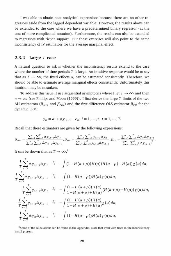
I was able to obtain neat analytical expressions because there are no other re-gressors aside from the lagged dependent variable. However, the results above canbe extended to the case where we have a predetermined binary regressor (at thecost of more complicated notation). Furthermore, the results can also be extendedto regressors with richer support. But these exercises will also point to the sameinconsistency of IV estimators for the average marginal effect.

2.3.2 Large-T case

A natural question to ask is whether the inconsistency results extend to the casewhere the number of time periods T is large. An intuitive response would be to saythat as T → ∞, the fixed effects αi can be estimated consistently. Therefore, weshould be able to estimate average marginal effects consistently. Unfortunately, thisintuition may be mistaken.

To address this issue, I use sequential asymptotics where I let T →∞ and thenn→∞ (see Phillips and Moon (1999)). I first derive the large-T limits of the twoAH estimators (bρAHd and bρAHl) and the first-difference OLS estimator bρF D for thedynamic LPM:

yi t = αi +ρ yi,t−1 + εi t , i = 1, . . . , n, t = 1, . . . , T.

Recall that these estimators are given by the following expressions:

bρAHd =

∑ni=1

∑Tt=3∆yi,t−2∆yi t

∑ni=1

∑Tt=3∆yi,t−2∆yi,t−1

, bρAHl =

∑ni=1

∑Tt=2 yi,t−2∆yi t

∑ni=1

∑Tt=2 yi,t−2∆yi,t−1

, bρF D =

∑ni=1

∑Tt=2∆yi t∆yi,t−1

∑ni=1

∑Tt=2

∆yi,t−1

2 .

It can be shown that as T →∞,8

1T

T∑

t=3

∆yi,t−2∆yi tp→ −

ˆ(1−H (α+ρ))H (α) (H (α+ρ)−H (α)) g (α) dα,

1T

T∑

t=3

∆yi,t−2∆yi,t−1p→ −

ˆ(1−H (α+ρ))H (α) g (α) dα,

1T

T∑

t=2

yi,t−2∆yi tp→ −

ˆ(1−H (α+ρ))H (α)1−H (α+ρ) +H (α)

(H (α+ρ)−H (α)) g (α) dα,

1T

T∑

t=2

yi,t−2∆yi,t−1p→ −

ˆ(1−H (α+ρ))H (α)1−H (α+ρ) +H (α)

g (α) dα,

1T

T∑

t=2

∆yi t∆yi,t−1p→ −

ˆ(1−H (α+ρ))H (α) g (α) dα,

8Some of the calculations can be found in the Appendix. Note that even with fixed n, the inconsistencyis still present.

28

1T

T∑

t=2

∆yi,t−1

2 p→ −2

ˆ(1−H (α+ρ))H (α)1−H (α+ρ) +H (α)

g (α) dα.

Notice that the limiting quantities above do not depend on i. Therefore, as n→∞,we must have

bρAHdp→ˆ

wd (α,ρ) (H (α+ρ)−H (α)) dα, (2.3.4)

bρAHlp→ˆ

wl (α,ρ) (H (α+ρ)−H (α)) dα, (2.3.5)

bρF Dp→

12

1−ˆ

wl (α,ρ) (H (α+ρ)−H (α)) dα

, (2.3.6)

where the weighting functions are given by

wd (α,ρ) =H (α) (1−H (α+ρ)) g (α)ˆH (α) (1−H (α+ρ)) g (α) dα

,

wl (α,ρ) =

(1−H (α+ρ))H (α)1−H (α+ρ) +H (α)

g (α)ˆ(1−H (α+ρ))H (α)1−H (α+ρ) +H (α)

g (α) dα.

As for the behavior of the fixed effects (FE) estimator in the large-T case, I rely onProposition 3.1 of Galvao and Kato (2014). In the context I consider, the linear prob-ability model is misspecified and the true model is the nonlinear model (2.3.1). Asa result, the conditional mean E

yi t |yi,t−1,αi

is misspecified as additive and linearwhen in fact it is nonlinear. Under their assumptions A1 to A3, they show that theFE estimator converges to the following pseudo-true parameter:

β0 =E

eyi t eyi,t−1

E

ey2i,t−1

,

where eyi t = yi t − E

yi t |yi,t−1,αi

. Assumption A1 of their paper require that themarginal distribution of

αi , yi t , yi,t−1

is invariant with respect to (i, t). As a re-sult, the initial condition is drawn from the stationary distribution conditional onαi . Notice that I did not impose this assumption. In the appendix, I show that thispseudo-true parameter is given by

β0 =E

(H (α+ρ)−H (α))Pr

yi,t−1 = 1|α

1− Pr

yi,t−1 = 1|α

E

Pr

yi,t−1 = 1|α

1− Pr

yi,t−1 = 1|α , (2.3.7)

where the expectations are calculated with respect to the marginal distribution of α.

29

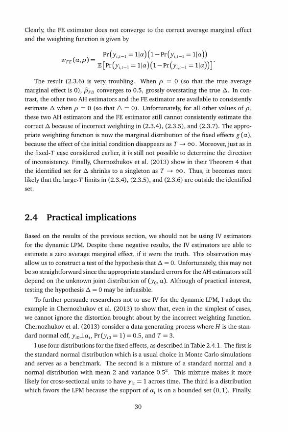
Clearly, the FE estimator does not converge to the correct average marginal effectand the weighting function is given by

wF E (α,ρ) =Pr

yi,t−1 = 1|α

1− Pr

yi,t−1 = 1|α

E

Pr

yi,t−1 = 1|α

1− Pr

yi,t−1 = 1|α .

The result (2.3.6) is very troubling. When ρ = 0 (so that the true averagemarginal effect is 0), bρF D converges to 0.5, grossly overstating the true ∆. In con-trast, the other two AH estimators and the FE estimator are available to consistentlyestimate ∆ when ρ = 0 (so that 4 = 0). Unfortunately, for all other values of ρ,these two AH estimators and the FE estimator still cannot consistently estimate thecorrect∆ because of incorrect weighting in (2.3.4), (2.3.5), and (2.3.7). The appro-priate weighting function is now the marginal distribution of the fixed effects g (α),because the effect of the initial condition disappears as T →∞. Moreover, just as inthe fixed-T case considered earlier, it is still not possible to determine the directionof inconsistency. Finally, Chernozhukov et al. (2013) show in their Theorem 4 thatthe identified set for ∆ shrinks to a singleton as T →∞. Thus, it becomes morelikely that the large-T limits in (2.3.4), (2.3.5), and (2.3.6) are outside the identifiedset.

2.4 Practical implications

Based on the results of the previous section, we should not be using IV estimatorsfor the dynamic LPM. Despite these negative results, the IV estimators are able toestimate a zero average marginal effect, if it were the truth. This observation mayallow us to construct a test of the hypothesis that∆= 0. Unfortunately, this may notbe so straightforward since the appropriate standard errors for the AH estimators stilldepend on the unknown joint distribution of (y0,α). Although of practical interest,testing the hypothesis ∆= 0 may be infeasible.

To further persuade researchers not to use IV for the dynamic LPM, I adopt theexample in Chernozhukov et al. (2013) to show that, even in the simplest of cases,we cannot ignore the distortion brought about by the incorrect weighting function.Chernozhukov et al. (2013) consider a data generating process where H is the stan-dard normal cdf, yi0⊥αi , Pr (yi0 = 1) = 0.5, and T = 3.

I use four distributions for the fixed effects, as described in Table 2.4.1. The first isthe standard normal distribution which is a usual choice in Monte Carlo simulationsand serves as a benchmark. The second is a mixture of a standard normal and anormal distribution with mean 2 and variance 0.52. This mixture makes it morelikely for cross-sectional units to have yi t = 1 across time. The third is a distributionwhich favors the LPM because the support of αi is on a bounded set (0,1). Finally,

30

the fourth is a mixture of two normals with negative means. This mixture achievesthe opposite effect compared to the second mixture.

Table 2.4.1: Distribution of fixed effects for computations

0.5N (0,1)+ 0.5N (−2, 0.1)+N (0, 1) 0.5N (2,0.5) Beta (4,2) 0.5N (−1, 1)

Mean 0 1 0.667 -1.5Variance 1 1.625 0.032 0.755Skewness 0 -0.543 -0.468 1.132Kurtosis 3 2.402 2.625 4.070

Multimodal? Unimodal Bimodal Unimodal Bimodal

In Figure 2.4.1, I calculate9 the large-n limits of the AH estimators (in blue forbρAHd and green for bρAHl) and large-n limits of the nonparametric bounds proposedby Chernozhukov et al. (2013) (in red for the lower bound ∆l and orange for theupper bound ∆u) evaluated at different values of ρ ∈ [−2,2]. I also calculate thetrue ∆ (in black) using the true distribution of (y0,α).

Even in the benchmark case where αi ∼ N (0,1), both the large-n limits of the AHestimators are larger than ∆ when ρ > 0. Further note that when ρ < −0.510, boththese large-n limits are outside the identified set. For αi ∼ 0.5N (0, 1)+0.5N (2,0.5),both the large-n limits of the AH estimators nearly coincide and are much larger than∆ even for less persistent state dependence. For αi ∼ Beta (4, 2), the large-n limitsof the AH estimators are practically the same as ∆ and both can be found in theidentified set. The key seems to be that the bounded support for the fixed effect,which is (0,1). Finally, the large-n limit of the AH estimator using levels as theinstrument set is smaller than ∆ for αi ∼ 0.5N (−2,0.1) + 0.5N (−1,1).

Although I do not have analytical results for GMM applied to the dynamic LPM, Iillustrate why GMM may not be a good idea using the empirical application by Cher-nozhukov et al. (2013) on female labor force participation and fertility. They esti-mate the following model using complete longitudinal data on 1587 married womenselected from the National Longitudinal Survey of Youth 1979 and observed for threeyears – 1990, 1992, and 1994:

LF Pi t = 1 (β · kidsi t +αi ≥ εi t) .

The parameter of interest is the average marginal effect of fertility on female laborforce participation. The dependent variable is a labor force participation indicator,

9A Mathematica notebook containing the calculations is available at http://andrew-pua.ghost.io.

10Negative state dependence has been found in the literature on scarring effects (see references inTorgovitsky (2015)).

31

the regressor is a fertility indicator that takes the value 1 if the woman has a childless than 3 years old, and αi is the individual-specific fixed effect.

Chernozhukov et al. (2013) compute nonparametric bounds for the average marginaleffect under the assumption that the fertility indicator is strictly exogenous (calledstatic bounds) and that the average marginal effect is decreasing11 in the fertility in-dicator. I replicate their bounds and they can be found in row (2) of Table 2.4.3. I alsoinclude static bounds without monotonicity for comparison in row (1).12 In addition,I compute two other nonparametric bounds with and without the monotonicity as-sumption under the assumption that the fertility indicator is predetermined (calleddynamic bounds) in rows (3) and (4).

Table 2.4.3: Female LFP and fertility (n= 1587, T = 3)

Avg. Marginal Effect 95% CI(1) Static NP bounds [−0.40, 0.09](2) (1) under monotonicity [−0.40,−0.04](3) Dynamic NP bounds [−0.39, 0.11](4) (3) under monotonicity [−0.39,−0.19](5) Random effects probit −0.11 [−0.13,−0.08](6) Fixed effects OLS −0.08 [−0.11,−0.06](7) First-difference OLS −0.08 [−0.09,−0.04](8) AH (differences) −0.01 [−0.14, 0.13](9) AH (levels) −0.02 [−0.07, 0.03](10) Arellano-Bond −0.02 [−0.07, 0.03]

I also report estimates based on the linear probability model along with the usual95% asymptotic confidence intervals. Both the fixed effects and first-differenced esti-mates (rows (6) and (7)) can be found inside the static bounds. This is no longer thecase when static bounds are computed under the monotonicity assumption. In con-trast, the estimated average marginal effect from the random effects probit (row (5))is inside the static bounds with or without monotonicity, despite the very incredibleassumption where the fixed effects are independent of the fertility indicator. Finally,note that the AH and Arellano-Bond estimates (rows (8) to (10)), which actuallyassume predeterminedness, are outside the dynamic bounds under monotonicity.

11Details as to how to construct the bounds under monotonicity can be found in the SupplementalMaterial to Chernozhukov et al. (2013).

12A Stata do-file is available for replication at http://andrew-pua.ghost.io.

32

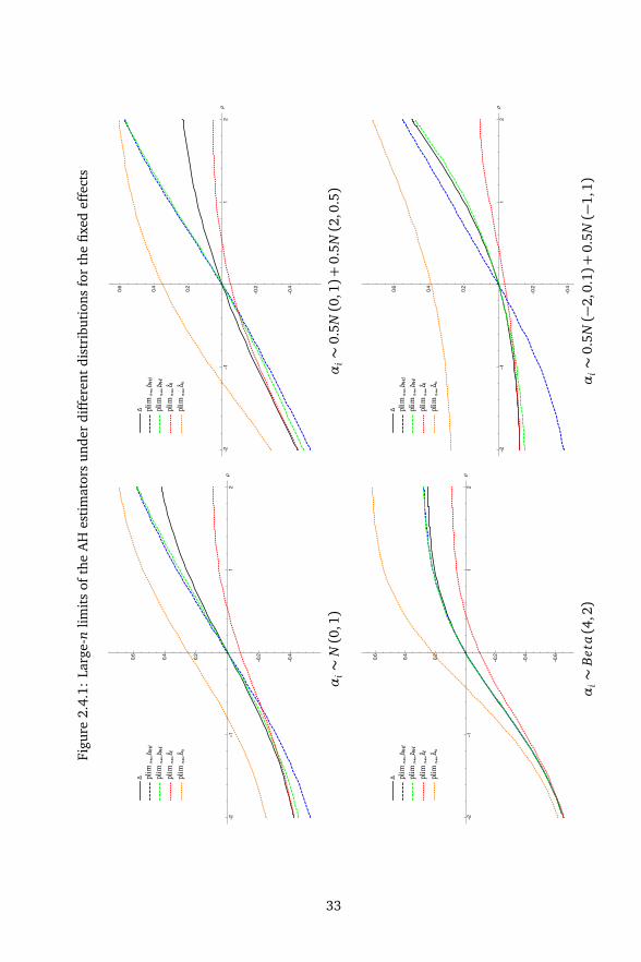
Figu

re2.

4.1:

Larg

e-n

limit

sof

the

AH

esti

mat

ors

unde

rdi

ffer

ent

dist

ribu

tion

sfo

rth

efix

edef

fect

s

αi∼

N(0

,1)

αi∼

0.5N(0

,1)+

0.5N(2

,0.5)

αi∼

Bet

a(4

,2)

αi∼

0.5N(−

2,0.

1)+

0.5N(−

1,1)

33

2.5 Concluding remarks

I show that using IV methods to estimate the dynamic LPM with fixed effects is in-appropriate even in large samples (whether n or T diverge). The analytical resultsindicate that incorrect weighting of the individual treatment effect is the source ofthe problem. The numerical results indicate that the estimators may be outside theidentified set in both finite and large samples. Therefore, it is more appropriate touse the nonparametric bounds proposed by Chernozhukov et al. (2013), especiallyif one is unwilling to specify the form for the inverse link function and the jointdistribution of the initial conditions and the fixed effects.

The large-n, large-T results I obtain are based on sequential asymptotics. I conjec-ture that we should obtain similar inconsistency results based on joint asymptotics.It is also unclear whether bias corrections that are derived under large-n, large-Tasymptotics can be directly applied to the dynamic LPM with fixed effects. The re-sults in the paper point out that the direction of the asymptotic bias of the estimatorfor the average marginal effect cannot be obtained. This in stark contrast with thedirection of the asymptotic bias derived by Nickell (1981). Although the Monte Carloexperiments of Fernandez-Val (2009) indicate good finite sample performance whenwe apply the large-T bias corrections, future work should study what exactly thesecorrections are doing.

It would also be interesting to derive similar analytical results for correlated ran-dom effects models so that the results in Wooldridge (2005a) and Murtazashvili andWooldridge (2008) can be extended to the dynamic case. In the empirical applica-tion, I find that the average marginal effect from the usual random effects probitunder strict exogeneity can be found in the static nonparametric bounds. Respect-ing the inherent nonlinearity of a discrete choice model may be responsible for thisfinding. Future work on this will be of practical interest.

2.6 Appendix

Some calculations for (2.3.3)

We calculate E [1 (yi0 = 0, yi1 = 1, yi2 = 1, yi3 = 0)] in detail since the other expres-sions follow similarly. This expression is equal to

Pr (yi0 = 0, yi1 = 1, yi2 = 1, yi3 = 0)

=ˆ

Pr (yi0 = 0, yi1 = 1, yi2 = 1, yi3 = 0|α) g (α) dα

=ˆ

Pr (yi3 = 0|yi0 = 0, yi1 = 1, yi2 = 1,α)Pr (yi2 = 1|yi0 = 0, yi1 = 1,α)×

Pr (yi1 = 1|yi0 = 0,α)Pr (yi0 = 0|α) g (α) dα

34

=ˆ

Pr (yi3 = 0|yi2 = 1,α)Pr (yi2 = 1|yi1 = 1,α)

×Pr (yi1 = 1|yi0 = 0,α) f (α, 0) dα

=ˆ(1−H (α+ρ))H (α+ρ)H (α) f (α, 0) dα, (2.6.1)

where f is the joint density of (α, y0). Similarly, we have the following:

E [1 (yi0 = 1, yi1 = 0, yi2 = 0, yi3 = 1)] =ˆ

H (α) (1−H (α)) (1−H (α+ρ)) f (α, 1) dα

E [1 (yi0 = 1, yi1 = 0, yi2 = 1, yi3 = 0)] =ˆ(1−H (α+ρ))H (α) (1−H (α+ρ)) f (α, 1) dα

E [1 (yi0 = 0, yi1 = 1, yi2 = 0, yi3 = 1)] =ˆ

H (α) (1−H (α+ρ))H (α) f (α, 0) dα

E [1 (yi0 = 0, yi1 = 1, yi2 = 0, yi3 = 0)] =ˆ(1−H (α)) (1−H (α+ρ))H (α) f (α, 0) dα

E [1 (yi0 = 1, yi1 = 0, yi2 = 1, yi3 = 1)] =ˆ

H (α+ρ)H (α) (1−H (α+ρ)) f (α, 1) dα

Assembling these expressions together in the expression for the large-sample limit ofbρAHd gives (2.3.3).

Some calculations for the large-T case

Note that ∆yi,t−2∆yi t = yi,t−2 yi t − yi,t−3 yi t − yi,t−2 yi,t−1+ yi,t−3 yi,t−1. Observe thatthe binary nature of y allows us to write

1T

T∑

t=3

yi,t−2 yi tp→ lim

T→∞

1T

T∑

t=3

Pr

yi t = 1, yi,t−2 = 1

.

By the law of total probability, the definition of conditional probability, and calcula-tions similar to (2.6.1), we are able to express Pr

yi t = 1, yi,t−2 = 1

as

Pr

yi t = 1, yi,t−2 = 1

= Pr

yi t = 1, yi,t−1 = 0, yi,t−2 = 1

+ Pr

yi t = 1, yi,t−1 = 1, yi,t−2 = 1

=ˆ

H (α) (1−H (α+ρ))Pr

yi,t−2 = 1|α

g (α) dα

+ˆ

H (α+ρ)2 Pr

yi,t−2 = 1|α

g (α) dα.

As a result, we have

1T

T∑

t=3

yi,t−2 yi tp→ˆ

H (α+ρ)2 +H (α) (1−H (α+ρ))

limT→∞

1T

T∑

t=3

Pr

yi,t−2 = 1|α

g (α) dα.

35

Finally observe that Pr

yi,t−2 = 1|α

obeys a first-order nonhomogeneous differenceequation. In particular, note that

Pr (yi1 = 1|α) = Pr (yi1 = 1|yi0 = 1,α)Pr (yi0 = 1|α)

+Pr (yi1 = 1|yi0 = 0,α)Pr (yi0 = 0|α)

= [H (α+ρ)−H (α)]Pr (yi0 = 1|α) +H (α)

Pr (yi2 = 1|α) = Pr (yi2 = 1|yi1 = 1,α)Pr (yi1 = 1|α)

+Pr (yi2 = 1|yi1 = 0,α)Pr (yi1 = 0|α)

= [H (α+ρ)−H (α)]Pr (yi1 = 1|α) +H (α)...

Pr (yi t = 1|α) = [H (α+ρ)−H (α)]Pr

yi,t−1 = 1|α

+H (α)

The solution to the above difference equation can be written as

Pr (yi t = 1|α) = [H (α+ρ)−H (α)]t Pr (yi0 = 1|α)+t−1∑

s=0

[H (α+ρ)−H (α)]s H (α) .

Note that |H (α+ρ)−H (α)| < 1. As a result, the effect of the initial conditiondisappears as T →∞:

limT→∞

1T

T∑

t=3

Pr

yi,t−2 = 1|α

=H (α)

1−H (α+ρ) +H (α).

Thus, we have

1T

T∑

t=3

yi,t−2 yi tp→ˆ

H (α+ρ)2 +H (α) (1−H (α+ρ))

H (α)1−H (α+ρ) +H (α)

g (α) dα.

Following similar calculations, we can derive the large-T limits of the other compo-nents. In particular,

1T

T∑

t=3

yi,t−2 yi,t−1p→ lim

T→∞

1T

T∑

t=3

Pr

yi,t−1 = 1, yi,t−2 = 1

=ˆ

H (α+ρ)

H (α)1−H (α+ρ) +H (α)

g (α) dα.

1T

T∑

t=3

yi,t−3 yi tp→ lim

T→∞

1T

T∑

t=3

Pr

yi t = 1, yi,t−3 = 1

=ˆ

H (α+ρ)3

H (α)1−H (α+ρ) +H (α)

g (α) dα

+ˆ

2H (α+ρ)H (α) (1−H (α+ρ))

H (α)1−H (α+ρ) +H (α)

g (α) dα

36

+ˆ

H (α) (1−H (α)) (1−H (α+ρ))

H (α)1−H (α+ρ) +H (α)

g (α) dα.

Observe that the last term1T

T∑

t=3

yi,t−3 yi,t−1

has the same probability limit as

1T

T∑

t=3

yi,t−2 yi,t

as T →∞. Assembling all the results together, we have as T →∞,

1T

T∑

t=3

∆yi,t−2∆yi tp→−ˆ(1−H (α+ρ))H (α) (H (α+ρ)−H (α)) g (α) dα.

The other large-T results now follow similar computations.

Derivation of the large-n, large-T limit of the fixed effects estima-tor

Galvao and Kato (2014) impose assumptions A1 to A3 to derive the large-n, large-T limit of the fixed effects estimator. Assumption A1 is about independence acrosscross-sectional units and a mild form of time series dependence conditional on αi .For my case, I needed to impose the assumption that the initial condition is drawnfrom its stationary distribution conditional on αi , unlike the derivations for the AHestimators.

Let eyi t = yi t −E (yi t = 1|αi) = yi t − Pr (yi t = 1|αi) for t = 1, . . . , T . AssumptionA2 is about the existence and boundedness of the moments of eyi t . These momentsare guaranteed to exist and be bounded because eyi t has a Bernoulli distributionwith probability Pr (yi t = 1|αi) ∈ (0, 1). They show that the fixed effects estimatorconverges to the following pseudo-true parameter:

β0 =E

eyi t eyi,t−1

E

ey2i,t−1

.

I now calculate the denominator explicitly. First, note that

ey2i,t−1 = y2

i,t−1 − 2yi,t−1 Pr

yi,t−1 = 1|αi

+

Pr

yi,t−1 = 1|αi

2

= yi,t−1 − 2yi,t−1 Pr

yi,t−1 = 1|αi

+

Pr

yi,t−1 = 1|αi

2.

37

Taking expectations, we have

E

ey2i,t−1

= E

yi,t−1 − 2yi,t−1 Pr

yi,t−1 = 1|αi

+

Pr

yi,t−1 = 1|αi

2

= E

E

yi,t−1|αi

− 2E

yi,t−1|αi

Pr

yi,t−1 = 1|αi

+

Pr

yi,t−1 = 1|αi

2

= E

Pr

yi,t−1 = 1|αi

−

Pr

yi,t−1 = 1|αi

2

= E

Pr

yi,t−1 = 1|αi

1− Pr

yi,t−1 = 1|αi

.

Note that E

ey2i,t−1

> 0 and satisfies assumption A3 of Galvao and Kato (2014). Asfor the numerator, note that

eyi t eyi,t−1 = yi t yi,t−1 − yi t Pr

yi,t−1 = 1|αi

− yi,t−1 Pr (yi t = 1|αi)

+Pr (yi t = 1|αi)Pr

yi,t−1 = 1|αi

. (2.6.2)

Take the first two terms of the right hand side of (2.6.2). Applying law of iteratedexpectations and E

yi t |yi,t−1,αi

= Pr

yi t = 1|yi,t−1,αi

gives

E

yi,t−1 − Pr

yi,t−1 = 1|αi

yi t

= E

E

E

yi,t−1 − Pr

yi,t−1 = 1|αi

yi t |yi,t−1,αi

|αi

= E

E

yi,t−1 − Pr

yi,t−1 = 1|αi

E

yi t |yi,t−1,αi

|αi

= E

E

yi,t−1 − Pr

yi,t−1 = 1|αi

H

αi +ρ yi,t−1

|αi

= E

1− Pr

yi,t−1 = 1|αi

H (αi +ρ)Pr

yi,t−1 = 1|αi

−E

Pr

yi,t−1 = 1|αi

H (αi)

1− Pr

yi,t−1 = 1|αi

.

The last two terms of the right hand side of (2.6.2) is equal to zero. As a result, weobtain

E

eyi t eyi,t−1

= E

(H (αi +ρ)−H (αi))Pr

yi,t−1 = 1|αi

1− Pr

yi,t−1 = 1|αi

.

Combining all these findings give us the final form for the pseudo-true parameter:

β0 =E

(H (αi +ρ)−H (αi))Pr

yi,t−1 = 1|αi

1− Pr

yi,t−1 = 1|αi

E

Pr

yi,t−1 = 1|αi

1− Pr

yi,t−1 = 1|αi

.

38

Chapter 3

Simultaneous equationsmodels for discrete outcomes:Coherence and completenessusing panel data

3.1 Introduction

In this chapter, I show how to estimate a dynamic simultaneous equations panel datamodel with discrete outcomes. There are two main issues involved in this endeavor,namely, the manner in which time-invariant unobserved heterogeneity is introducedand the manner in which the nonexistence of a unique reduced form is addressed.Both these issues have implications for how the parameters of the simultaneous equa-tions model are going to be identified and estimated. I show how both these issuescan be tackled at the same time.

Researchers who want to estimate a dynamic simultaneous equations model withdiscrete outcomes using panel data would have to introduce an additive individual-specific fixed effect into the latent index. Unfortunately, time-invariant unobservedheterogeneity cannot be left unrestricted in dynamic nonlinear panel data models,especially when the number of time periods T is small (see Section 4 of Arellano andBonhomme (2011)). Although we have bias reduction procedures for parameters ofinterest, they are motivated from a large-T perspective. Results of existing MonteCarlo simulations for dynamic nonlinear panel data models indicate that T has to bemuch larger than 10 in order to reap the gains from bias reduction (see Bester andHansen (2009a), Carro (2007), Fernandez-Val (2009), and Hahn and Kuersteiner

39

(2011)). Furthermore, the fixed-T solution proposed by Bonhomme (2012) onlyapplies to models without dynamics. As a compromise, we have to restrict somefeatures of the distribution of time-invariant unobserved heterogeneity. Allowingfor fixed effects in these models has not been explored fully, since most researchhas focused on either cross-sectional models, continuous outcomes (or the latentoutcomes themselves), or random effects (for examples, see the work by Cornwell,Schmidt, and Wyhowski (1992), Leon-Gonzalez (2003), Matzkin (2008), Matzkin(2012), and Masten (2015)).

Even if T is large, coherency conditions would still have to be imposed. Co-herency conditions effectively convert a model where the endogenous variables arejointly determined into a model which is triangular or recursive. A triangular modelrestricts the direction in which an endogenous variable affects other endogenousvariables (for all observations). Triangularity implies that there are either zero or in-equality restrictions on the parameters or functions of the parameters. For example,when there are two binary endogenous variables y1 and y2 that are jointly deter-mined, y2 should not enter the equation for y1 or vice-versa. As a result, we have tochoose beforehand how the coherency conditions should be imposed.

The literature on coherency conditions started with research aiming to extendthe simultaneous equations approach of the Cowles Commission to endogenous vari-ables that are subject to censoring or truncation. Some representative papers in thisarea include Maddala and Lee (1976), Heckman (1978), Gourieroux, Laffont, andMonfort (1980), and Schmidt (1981). Blundell and Smith (1993) summarize thisstrand of the literature. They have all shown that parameter restrictions are typ-ically required to ensure the existence and uniqueness of the reduced form. As aresult, ensuring coherency is a first step prior to discussing identification. Later re-search has focused more on how to avoid imposing the coherency conditions (seethe contribution of Tamer (2003)).

In order to avoid imposing these coherency conditions, a separate strand of theliterature has emphasized that the uniqueness of equilibrium in game-theoretic mod-els has parallels with the problems involving uniqueness of the reduced form forsimultaneous equation models with discrete outcomes. Early work in the estima-tion of game-theoretic models such as Bjorn and Vuong (1984), Bresnahan and Reiss(1991), and Kooreman (1994) attempt to overcome the possibility of multiple equi-libria either by introducing a selection mechanism which assumes that players chooseone of the equilibria at random or by fusing multiple equilibria as one outcome.Tamer (2003) shows that point identification and consistent estimation is still pos-sible without imposing a set of auxiliary assumptions that resolve the underlyingmultiplicity. All that is needed is the presence of a regressor with large support. Hesuggests a semiparametric ML estimator that is more efficient than the ML estimatorthat fuses multiple equilibria as one outcome. In fact, Tamer (2003) introduces newterminology to differentiate models whose reduced form is nonexistent and models

40

whose reduced form is nonunique. He calls these models incoherent and incomplete,respectively. Note that these cited papers focus on the incompleteness aspect becausethe signs of some parameters of game-theoretic models may be known a priori. Thesesign restrictions effectively rule out potential incoherence of the model.

Some like Dagenais (1999), Massacci (2010), and Hajivassiliou and Savignac(2011) have attempted to resolve both incompleteness and incoherence by imposingerror-support restrictions. They all offer estimation methods that involve reweight-ing the likelihood contributions to reflect the restrictions on the error supports. Inthe most recent work by Chesher and Rosen (2012), they show how identified setscan be constructed without resorting to the restriction of error supports and a priorisign restrictions at all. In the process of constructing these identified sets, they wereable to unify the different approaches that are available in the literature in the mostgeneral way possible. With the exception of Hajivassiliou and Savignac (2011), thepreceding papers focus on either cross-sectional or time-series settings. On the otherhand, Hajivassiliou and Savignac (2011) use panel data to estimate a model of thejoint determination of a firm’s decision to innovate and a firm’s exposure to highercredit constraints but do not allow for fixed effects.

My proposal approaches the problem of incompleteness and incoherence froma different perspective. I exploit Lewbel’s (2007) characterization of coherence andcompleteness when one of the endogenous variables is binary. He shows that a possi-ble characterization involves indexing the direction of causality by a dummy variablewhich may be observable or modeled. In contrast, I do not restrict the dependenceon observables but assume that this dependence is individual-specific. As a result, Iallow for the estimation of a panel data simultaneous equations model with discreteoutcomes where the individual-specific fixed effect can be interpreted as the mannerin which the coherency condition holds or the direction in which causality flows fromone discrete endogenous variable to another.

The paper is organized as follows. In Section 3.2, I provide a motivating exampleto demonstrate my proposal. In Section 3.3, I discuss how identification, estimationand inference may proceed in the model considered by Hajivassiliou and Ioannides(2007) (henceforth, HI). In Section 3.4, I revisit the empirical application of HI andcast doubt on the coherency conditions they have imposed. I conclude and suggestavenues for further work in Section 3.5.

3.2 A stylized example

3.2.1 Coherence and completeness

I start by introducing some terminology in the context of a simple example. Con-sider the situation where two dummy variables are jointly determined. This situationtypically arises in many empirical applications, such as determining whether binary

41

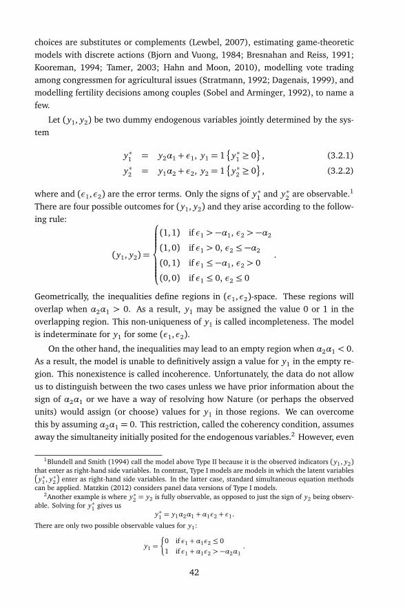
choices are substitutes or complements (Lewbel, 2007), estimating game-theoreticmodels with discrete actions (Bjorn and Vuong, 1984; Bresnahan and Reiss, 1991;Kooreman, 1994; Tamer, 2003; Hahn and Moon, 2010), modelling vote tradingamong congressmen for agricultural issues (Stratmann, 1992; Dagenais, 1999), andmodelling fertility decisions among couples (Sobel and Arminger, 1992), to name afew.

Let (y1, y2) be two dummy endogenous variables jointly determined by the sys-tem

y∗1 = y2α1 + ε1, y1 = 1

y∗1 ≥ 0

, (3.2.1)

y∗2 = y1α2 + ε2, y2 = 1

y∗2 ≥ 0

, (3.2.2)

where and (ε1,ε2) are the error terms. Only the signs of y∗1 and y∗2 are observable.1

There are four possible outcomes for (y1, y2) and they arise according to the follow-ing rule:

(y1, y2) =

(1,1) if ε1 > −α1, ε2 > −α2

(1,0) if ε1 > 0, ε2 ≤ −α2

(0,1) if ε1 ≤ −α1, ε2 > 0

(0,0) if ε1 ≤ 0, ε2 ≤ 0

.

Geometrically, the inequalities define regions in (ε1,ε2)-space. These regions willoverlap when α2α1 > 0. As a result, y1 may be assigned the value 0 or 1 in theoverlapping region. This non-uniqueness of y1 is called incompleteness. The modelis indeterminate for y1 for some (ε1,ε2).

On the other hand, the inequalities may lead to an empty region when α2α1 < 0.As a result, the model is unable to definitively assign a value for y1 in the empty re-gion. This nonexistence is called incoherence. Unfortunately, the data do not allowus to distinguish between the two cases unless we have prior information about thesign of α2α1 or we have a way of resolving how Nature (or perhaps the observedunits) would assign (or choose) values for y1 in those regions. We can overcomethis by assuming α2α1 = 0. This restriction, called the coherency condition, assumesaway the simultaneity initially posited for the endogenous variables.2 However, even

1Blundell and Smith (1994) call the model above Type II because it is the observed indicators (y1, y2)that enter as right-hand side variables. In contrast, Type I models are models in which the latent variables

y∗1 , y∗2

enter as right-hand side variables. In the latter case, standard simultaneous equation methodscan be applied. Matzkin (2012) considers panel data versions of Type I models.

2Another example is where y∗2 = y2 is fully observable, as opposed to just the sign of y2 being observ-able. Solving for y∗1 gives us

y∗1 = y1α2α1 +α1ε2 + ε1.

There are only two possible observable values for y1:

y1 =

0 if ε1 +α1ε2 ≤ 01 if ε1 +α1ε2 > −α2α1

.

42

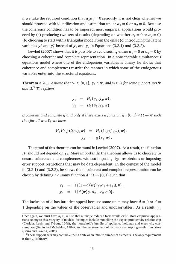
if we take the required condition that α2α1 = 0 seriously, it is not clear whether weshould proceed with identification and estimation under α1 = 0 or α2 = 0. Becausethe coherency condition has to be imposed, most empirical applications would pro-ceed by (a) producing two sets of results (depending on whether α1 = 0 or α2 = 0)(b) choosing to start with a triangular model from the onset (c) introducing the latentvariables y∗1 and y∗2 instead of y1 and y2 in Equations (3.2.1) and (3.2.2).

Lewbel (2007) shows that it is possible to avoid setting either α1 = 0 or α2 = 0 bychoosing a coherent and complete representation. In a nonseparable simultaneousequations model where one of the endogenous variables is binary, he shows thatcoherence and completeness restrict the manner in which some of the endogenousvariables enter into the structural equations:

Theorem 3.2.1. Assume that y1 ∈ 0,1, y2 ∈ Ψ, and w ∈ Ω for some support sets Ψand Ω.3 The system

y1 = H1 (y1, y2, w) ,

y2 = H2 (y1, y2, w)

is coherent and complete if and only if there exists a function g : 0, 1 ×Ω→ Ψ suchthat for all w ∈ Ω, we have

H1 (0, g (0, w) , w) = H1 (1, g (1, w) , w) ,

y2 = g (y1, w) .

The proof of this theorem can be found in Lewbel (2007). As a result, the functionH1 should not depend on y1. More importantly, the theorem allows us to choose g toensure coherence and completeness without imposing sign restrictions or imposingerror support restrictions that may be data-dependent. In the context of the modelin (3.2.1) and (3.2.2), he shows that a coherent and complete representation can bechosen by defining a dummy function d : Ω→ 0,1 such that

y1 = 1 (1− d (w)) y2α1 + ε1 ≥ 0 ,

y2 = 1 d (w) y1α2 + ε2 ≥ 0 .

The inclusion of d has intuitive appeal because some units may have d = 0 or d =1 depending on the values of the observables and unobservables. As a result, y1

Once again, we must have α2α1 = 0 so that a unique reduced form would exist. More empirical applica-tions belong to this category of models. Examples include modelling the export-productivity relationship(Clerides, Lach, and Tybout, 1998), the household’s bundle of appliance holdings and electricity con-sumption (Dubin and McFadden, 1984), and the measurement of recovery via output growth from crises(Cerra and Saxena, 2008).

3These support sets may contain either a finite or an infinite number of elements. The only requirementis that y1 is binary.

43

depends on y2 when d = 0 and y2 depends on y1 when d = 1. Unfortunately,Lewbel (2007) assumes that d is observable or could be modeled in some way.4

Note that Lewbel’s (2007) approach gives a new interpretation for simultaneitywhen compared to its traditional usage in econometrics. Instead of simultaneitybeing a purely structural aspect of the model, simultaneity arises because of theeconometrician’s inability to distinguish the direction of dependence (from y1 to y2

or vice versa). Intuitively, information from repeated measurements can be usefulin overcoming this inability without making parametric assumptions on the dummyfunction d.

In contrast to linear simultaneous equations models where there is a form of“bidirectional” causality (not in the usual Granger-causality sense) between two con-tinuously distributed variables, the models I consider only allow for one-directionalcausality from y1 to y2 for a subset of observations and one-directional causalityfrom y2 to y1 for the remaining set of observations. This is more credible than im-posing the coherency conditions which will ultimately result in either one-directionalcausality from y1 to y2 for all observations or one-directional causality from y2 to y1

for all observations, but not both.

The model in (3.2.1) and (3.2.2) can be thought of as a static discrete game ofcomplete information. In contrast to game-theoretic models, the models I considerallow for both incompleteness and incoherence. Incompleteness arising from multi-ple equilibria is a common feature in the estimation of game-theoretic models. Hahnand Moon (2010) estimate (3.2.1) and (3.2.2) using panel data of pairs of agentsusing Nash play. They assume that the model is incomplete by imposing sign restric-tions α1 < 0 and α2 < 0 and that pairs of agents choose one of the two equilibriaand stick to that same choice throughout time.

Since I am working with a complete and coherent representation by introducingd, it may be useful to motivate the representation in game-theoretic terms. Onecan view the representation as arising from the inability of the econometrician toobserve how multiple equilibria or absence of equilibrium was resolved, possiblythrough an unmodelled communication or coordination device. Alternatively, theeconometrician may also have neglected to model the sequential nature of the gameand was unable to observe which player moved first (but the agents are aware of thesequential nature of the game).

4Introducing this dummy function is just one way to obtain a coherent and complete representationwhenever one of the endogenous variables is binary. One could argue that this device may be useful in alinear simultaneous equations setting. A step in this direction is the introduction of random coefficientsin a linear simultaneous equations model (see Masten (2015) for more details).

44

3.2.2 Why a cross section is not enough

Suppose we treat d as unobservable. For the moment, assume we only have a cross-section of observations which form a random sample. Consider the model

y1i = 1 ((1− di) y2iα1 + ε1i ≥ 0) , (3.2.3)

y2i = 1 (di y1iα2 + ε2i ≥ 0) , (3.2.4)

for i = 1, . . . , n. Let Pr (di = 1) = pi and Pr (di = 0) = 1 − pi , where pi ∈ (0,1). Iassume that di , ε1i and ε2i are i.i.d. draws from their joint distribution. There arefour joint probabilities of the form Pr (y1i = j, y2i = k), where ( j, k) ∈ 0,1×0,1,that are observable from the data but only three of these provide restrictions on theparameters of the model (since all these four probabilities should sum up to one). Asa result, it is not possible to have point identification for all parameters, even if weset pi = p for all i. The main reason is that there are four parameters (α1,α2,ρ, p)to identify given the three joint probabilities obtained from the data.

To illustrate and simplify things further, assume normality56 for the errors givendi for all i, i.e.

ε1i

ε2i

di ∼ N

00

,

1 ρ

ρ 1

. (3.2.5)

As a result, we have

ε1i

ε2i

di = 0∼

ε1i

ε2i

di = 1,

i.e., (ε1i ,ε2i) is independent of di . The parameters of interest are α1, α2, and ρ.Note that for all ( j, k) ∈ 0, 1 × 0,1, we have

Pr (y1i = j, y2i = k) = Pr (y1i = j, y2i = k|di = 1) pi

+Pr (y1i = j, y2i = k|di = 0) (1− pi) .

Specifically, we have

Pr (y1i = 0, y2i = 0) = Pr (ε1i ≤ 0,ε2i ≤ 0; ρ) , (3.2.6)

Pr (y1i = 1, y2i = 0) = Pr (ε1i ≥ 0,ε2i ≤ −α2; ρ) pi +Pr (ε1i ≥ 0,ε2i ≤ 0; ρ) (1− pi) ,(3.2.7)

Pr (y1i = 0, y2i = 1) = Pr (ε1i ≤ −α1,ε2i ≥ 0; ρ) (1− pi) + Pr (ε1i ≤ 0,ε2i ≥ 0; ρ) pi .(3.2.8)

5Normality is not really required here. All that is required is a bivariate cdf that is strictly monotonicin ρ. In cases where ρ is not a correlation coefficient but some one-dimensional parameter that indexesdependence modelled via a copula. See Section 3.3 for more details.

6Bivariate normality of the errors can be thought of as a simple factor structure. In particular, ε1i canbe written as ε1i = ρε2i + vi where vi ∼ N

0,1−ρ2

, ε2i ∼ N (0,1), and ε2i is independent of vi .

45

The left hand sides of (3.2.6), (3.2.7), and (3.2.8) are observable from the data. Weare unable to observe the mixing probability pi . As long as we observe outcomes ofthe form (y1i = 0, y2i = 0) from the data,7 (3.2.6) can be used to identify ρ becausethe bivariate normal cdf is strictly monotonic in ρ (hence, the bivariate normal cdfis invertible with respect to ρ). This is in contrast with identification problems as-sociated with ρ as documented by Freedman and Sekhon (2010) and Meango andMourifie (2013) in the context of triangular models with a dummy endogenous re-gressor.

Since ρ is identified, we can treat it as known for the next step. In particular,we can now use (3.2.7) and (3.2.8) to identify whether (i) α1 ≤ 0 or α1 ≥ 0 and(ii) α2 ≤ 0 or α2 ≥ 0 . Whenever the cross-sectional frequency of (y1i = 1, y2i = 0)is less than or equal to Pr (ε1i ≥ 0,ε2i ≤ 0; ρ), we must have α2 ≥ 0. Similarly,showing that the cross-sectional frequency of (y1i = 0, y2i = 1) is less than or equalto Pr (ε1i ≤ 0,ε2i ≥ 0; ρ) allows us to conclude that α1 ≥ 0. The other cases followanalogously.

Unfortunately, we need external information to determine the grouping of everyith unit. One possible route is to impose pi = Pr (di = 1) = Pr (d = 1) = p for alli. Knowing the signs of α1,α2 allows us to determine the group to which all unitsbelong. There are four cases to consider as shown in Table 3.2.1.

Table 3.2.1: Group assignment rules for model (3.2.3) and (3.2.4)

Condition Ruleα1 ≥ 0, α2 ≥ 0 d = 0 iff frequency of y1i = 0 less than Pr (ε1i ≤ 0)

d = 1 iff frequency of y2i = 0 less than Pr (ε2i ≤ 0)

α1 ≤ 0, α2 ≤ 0 d = 0 iff frequency of y1i = 0 greater than Pr (ε1i ≤ 0)d = 1 iff frequency of y2i = 0 greater than Pr (ε2i ≤ 0)

α1 ≥ 0, α2 ≤ 0 d = 0 iff frequency of y1i = 0 less than Pr (ε1i ≤ 0)d = 1 iff frequency of y2i = 0 greater than Pr (ε2i ≤ 0)

α1 ≤ 0, α2 ≥ 0 d = 0 iff frequency of y1i = 0 greater than Pr (ε1i ≤ 0)d = 1 iff frequency of y2i = 0 less than Pr (ε2i ≤ 0)

Once we know whether d = 0 or d = 1 for all i, we are able to only point-identify either α1 or α2 but not both. Suppose d = 0 for the moment. SincePr (y1i = 0, y2i = 1|d = 0) = Pr (ε1i ≤ −α1,ε2i ≥ 0; ρ) and Pr (ε1i ≤ −α1,ε2i ≥ 0; ρ)is strictly decreasing in α1 for fixed ρ, we are able to point-identify α1. In con-trast, α2 is set-identified because d = 0 for all observations and we know the sign

7The extreme case where we do not observe any other outcome aside from (y1i = 0, y2i = 0) is ruledout.

46

of α2. Similarly, we are able to point-identify α2 from Pr (y1i = 1, y2i = 0|d = 1) =Pr (ε1i ≥ 0,ε2i ≤ −α2; ρ) but only set-identify α1.

3.2.3 Why panel data may be useful

At this point, panel data may be useful for point identification of all the parame-ters. We can introduce individual-specific effects through d to allow for unrestricteddependence on the observables in a time-invariant manner. Note that I do not in-troduce individual-specific effects as intercepts in the linear predictors. As a result,time-invariant variables or even variables that do not have too much variation overtime may be included in the model. In contrast, the usual way of introducing fixedeffects additively precludes the inclusion of time-invariant variables of interest.

If we had panel data and imposed the assumption that pi does not vary over time,we will be able to achieve point identification. Consider once again the model butthis time adapted to panel data:

y1i t = 1 ((1− di) y2i tα1 + ε1i t ≥ 0) ,

y2i t = 1 (di y1i tα2 + ε2i t ≥ 0) ,

for i = 1, . . . , n and t = 1, . . . , T . Let Pr (di = 1) = pi and Pr (di = 0) = 1− pi , wherepi ∈ (0, 1). I assume that di , ε1i t and ε2i t are i.i.d. draws from their joint distribution.Assume bivariate normality once again as in (3.2.5).8 Analogously, we have

Pr (y1i t = 0, y2i t = 0) = Pr (ε1i t ≤ 0,ε2i t ≤ 0; ρ) , (3.2.9)

Pr (y1i t = 1, y2i t = 0) = Pr (ε1i t ≥ 0,ε2i t ≤ −α2; ρ) pi+Pr (ε1i t ≥ 0,ε2i t ≤ 0; ρ) (1− pi) ,(3.2.10)

Pr (y1i t = 0, y2i t = 1) = Pr (ε1i t ≤ −α1,ε2i t ≥ 0; ρ) (1− pi)+Pr (ε1i t ≤ 0,ε2i t ≥ 0; ρ) pi .(3.2.11)

We now follow the same steps in the identification argument of the previous sub-section. Data on the observed frequencies of (y1i t = 0, y2i t = 0) for all i and t pointidentify ρ from (3.2.9). After plugging in the value of ρ from the previous step,(3.2.10) and (3.2.11) for all i and t can be used to identify the signs of α1,α2 asbefore. Once the signs are identified, we can modify the group assignment rules inTable 3.2.1. Instead of using cross-sectional variation, we use time series variation of

8In footnote 6, bivariate normality can be rewritten as a factor structure. In the panel data case, thepossibilities are richer. In particular, we may have ε1i t = λ1θi + v1i t and ε2i t = λ2θi + v2i t , where θiis an individual-specific factor. A similar idea appears in Cameron and Taber (2004). They impose arandom effects assumption on θi . It may be possible to modify the identification argument I present toallow for this. Unfortunately, the right hand side of Equation 3.2.9 will become an integral that dependson the distribution of θi . An identification argument based on the large-sample limit of the likelihoodfunction for observations where (y1i t = 0, y2i t = 0) may be used. It is unclear whether we can avoid thedistributional assumption on θi . Preliminary research by Khan, Maurel, and Zhang (2015) points to theidentifying power of factor structures in triangular discrete response models.

47

every unit to decide whether di = 0 or di = 1. Notice that d is now allowed to varyacross cross-sectional units. Data on the observed frequencies of (y1i t = 0, y2i t = 1)for all t and i such that di = 0 point-identify α1. Similarly, data on the observedfrequencies of (y1i t = 1, y2i t = 0) for all t and i such that di = 1 point-identify α2.

What I have shown is that point identification may be possible in a model whereboth (y1, y2) are dummy endogenous variables jointly determined by the system(3.2.1) and (3.2.2) without imposing sign restrictions, as long as we have access topanel data. The approach considered here is slightly different from the entry-exitgame estimated by Hahn and Moon (2010) using panel data. They impose sign re-strictions (motivated by economic theory) producing an incomplete game-theoreticmodel. In their model, the econometrician is unable to observe which equilibriumwas selected by the players but whichever equilibrium is selected becomes fixedacross time. The approach considered here is also different from Hajivassiliou andSavignac (2011). They do not have fixed effects and they restrict error supportsconditional on the restriction that both α1 and α2 must not have the same sign.

The intuition behind the identification argument in both the cross-section andpanel data case is to find a subset of the data unaffected by the mixing probabilitypi . I use this subset of the data to identify the common parameters except for α1

and α2. Deciding whether di = 0 or di = 1 depends on time series variation. Afterdeciding the grouping, α1 and α2 can now be point identified. It is important to notethat the number of groups is known in advance. Lewbel’s (2007) characterizationof complete and coherent two-equation systems ensure that the number of groups isfixed at 2.

There are extensions of situations that follow essentially the identification argu-ment above. For instance, the identification argument can be extended to the casewhere we have an intercept, strictly exogenous regressors, and lagged dependentvariables. Another possibility is for the error terms to have other known marginaldistributions linked by a parametric copula as in Han and Vytlacil (2015) but ex-tended to the panel data case. Finally, we can accommodate other discrete choicemodels such as the multinomial logit/probit and ordered logit/probit.

3.3 The model

3.3.1 Background

I now describe how to identify and estimate the parameters of the model to be usedin the empirical application. HI (2007) construct a model of a household head liv-ing in finite time who chooses consumption and hours worked subject to a liquidityconstraint and a quantity constraint on labor supply. As a consequence of liquidityconstraints, household heads cannot hold negative wealth at any time over the lifecycle. Furthermore, they may be subject to involuntary unemployment / underem-

48

ployment, voluntary employment, or involuntary overemployment. As a result, theycan be in one of the following situations – (a) they are able to work but are unableto reach their desired number of hours, (b) they are able to work at their desirednumber of hours, or (c) they are working beyond their desired level of hours. HI(2007) derive the solutions to the optimization problem faced by a representativehousehold. The solutions to the optimization problem represent the optimal path ofassets and hours worked over the life cycle of the household.

The econometrician is able to observe whether or not the household head is liq-uidity constrained, i.e., the liquidity constraint indicator Si t takes on the value 1 or 0,respectively. Household heads could be involuntarily overemployed (Ei t = −1), vol-untarily employed (Ei t = 0), or involuntarily unemployed / underemployed (Ei t =1). The authors describe how these indicators were constructed in their earlier paper(see HI (1995)).

Since these optimal paths of assets and hours worked are determined jointly overthe household’s life cycle, the econometric treatment would have to acknowledge theunderlying simultaneity. HI (2007) argue that one can either model the employmentconstraint indicator conditionally on the liquidity constraint indicator or vice versa.They further point out that this is consistent with the intertemporal two-stage bud-geting of households described in Blundell and Walker (1986). Clearly, Lewbel’s(2007) characterization can be exploited without us choosing the causal direction inadvance or by presenting two sets of results.

HI (2007) specify their dynamic simultaneous equations model as follows:

S∗i t = γ11Si,t−1 + γ12Si,t−2 +δ0Ei t +δ1Ei,t−1 +δ2Ei,t−2

+X1i tβbp + εbp

i t , (3.3.1)

E∗i t = γ21Ei,t−1 + γ22Ei,t−2 +κ0Si t +κ1Si,t−1 +κ2Si,t−2

+X2i tβop + εop

i t , (3.3.2)

Si t = 1

S∗i t ≥ 0

,

Ei t = −1

E∗i t < θ−+ 1

E∗i t > θ+

where θ− and θ+ are lower and upper thresholds. Just as in HI (2007), I also nor-malize θ+ = 0. Observe that all the employment status indicators should reallyenter as two dummies because there are three categories. For example, δ0Ei t can bedecomposed into δ011 Ei t = −1+ δ021 Ei t = 1. HI (1995; 2007) show that thecoherency conditions are (δ01 +δ02)κ0 = 0 and δ01δ02κ0 = 0. As a result, we eitherhave κ0 = 0 or δ01 = δ02 = 0. If we exploit Lewbel’s (2007) result, we need not im-pose these coherency conditions at all. Next, I show how to identify the parametersof their model without imposing coherency conditions.

49

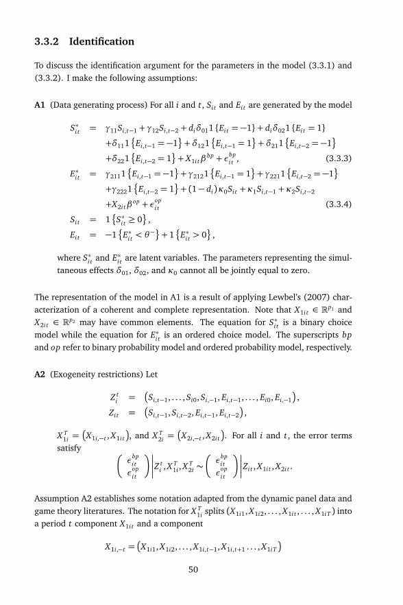
3.3.2 Identification

To discuss the identification argument for the parameters in the model (3.3.1) and(3.3.2). I make the following assumptions:

A1 (Data generating process) For all i and t, Si t and Ei t are generated by the model

S∗i t = γ11Si,t−1 + γ12Si,t−2 + diδ011 Ei t = −1+ diδ021 Ei t = 1

+δ111

Ei,t−1 = −1

+δ121

Ei,t−1 = 1

+δ211

Ei,t−2 = −1

+δ221

Ei,t−2 = 1

+ X1i tβbp + εbp

i t , (3.3.3)

E∗i t = γ2111

Ei,t−1 = −1

+ γ2121

Ei,t−1 = 1

+ γ2211

Ei,t−2 = −1

+γ2221

Ei,t−2 = 1

+ (1− di)κ0Si t +κ1Si,t−1 +κ2Si,t−2

+X2i tβop + εop

i t (3.3.4)

Si t = 1

S∗i t ≥ 0

,

Ei t = −1

E∗i t < θ−+ 1

E∗i t > 0

,

where S∗i t and E∗i t are latent variables. The parameters representing the simul-taneous effects δ01, δ02, and κ0 cannot all be jointly equal to zero.

The representation of the model in A1 is a result of applying Lewbel’s (2007) char-acterization of a coherent and complete representation. Note that X1i t ∈ Rp1 andX2i t ∈ Rp2 may have common elements. The equation for S∗i t is a binary choicemodel while the equation for E∗i t is an ordered choice model. The superscripts bpand op refer to binary probability model and ordered probability model, respectively.

A2 (Exogeneity restrictions) Let

Z ti =

Si,t−1, . . . , Si0, Si,−1, Ei,t−1, . . . , Ei0, Ei,−1

,

Zi t =

Si,t−1, Si,t−2, Ei,t−1, Ei,t−2

,

X T1i =

X1i,−t , X1i t

, and X T2i =

X2i,−t , X2i t

. For all i and t, the error termssatisfy

εbpi t

εopi t

Z ti , X T

1i , X T2i ∼

εbpi t

εopi t

Zi t , X1i t , X2i t .

Assumption A2 establishes some notation adapted from the dynamic panel data andgame theory literatures. The notation for X T

1i splits (X1i1, X1i2, . . . , X1i t , . . . , X1iT ) intoa period t component X1i t and a component

X1i,−t =

X1i1, X1i2, . . . , X1i,t−1, X1i,t+1 . . . , X1iT

50

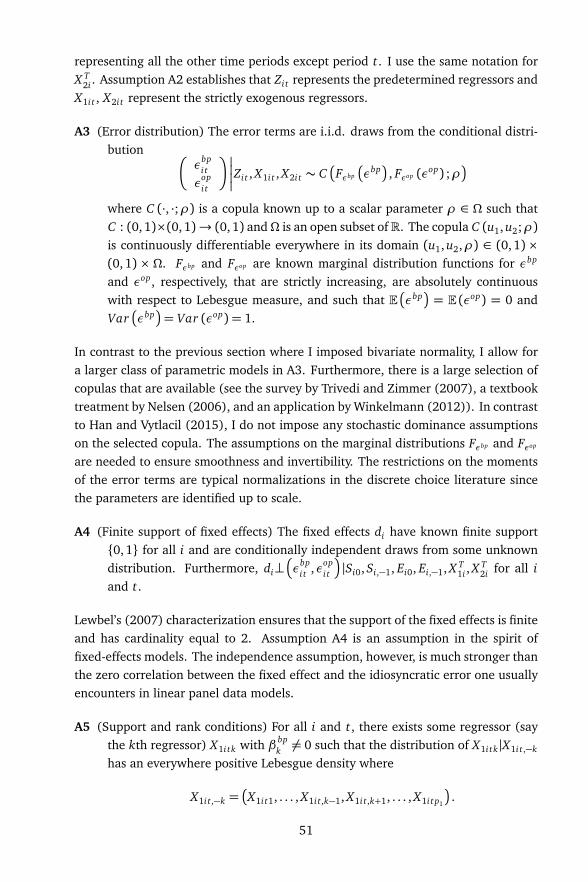
representing all the other time periods except period t. I use the same notation forX T

2i . Assumption A2 establishes that Zi t represents the predetermined regressors andX1i t , X2i t represent the strictly exogenous regressors.

A3 (Error distribution) The error terms are i.i.d. draws from the conditional distri-bution

εbpi t

εopi t

Zi t , X1i t , X2i t ∼ C

Fεbp

εbp

, Fεop (εop) ;ρ

where C (·, ·;ρ) is a copula known up to a scalar parameter ρ ∈ Ω such thatC : (0, 1)×(0, 1)→ (0, 1) andΩ is an open subset ofR. The copula C (u1, u2;ρ)is continuously differentiable everywhere in its domain (u1, u2,ρ) ∈ (0, 1) ×(0,1) × Ω. Fεbp and Fεop are known marginal distribution functions for εbp

and εop, respectively, that are strictly increasing, are absolutely continuouswith respect to Lebesgue measure, and such that E

εbp

= E (εop) = 0 andVar

εbp

= Var (εop) = 1.

In contrast to the previous section where I imposed bivariate normality, I allow fora larger class of parametric models in A3. Furthermore, there is a large selection ofcopulas that are available (see the survey by Trivedi and Zimmer (2007), a textbooktreatment by Nelsen (2006), and an application by Winkelmann (2012)). In contrastto Han and Vytlacil (2015), I do not impose any stochastic dominance assumptionson the selected copula. The assumptions on the marginal distributions Fεbp and Fεop

are needed to ensure smoothness and invertibility. The restrictions on the momentsof the error terms are typical normalizations in the discrete choice literature sincethe parameters are identified up to scale.

A4 (Finite support of fixed effects) The fixed effects di have known finite support0,1 for all i and are conditionally independent draws from some unknowndistribution. Furthermore, di⊥

εbpi t ,εop

i t

|Si0, Si,−1, Ei0, Ei,−1, X T1i , X T

2i for all iand t.

Lewbel’s (2007) characterization ensures that the support of the fixed effects is finiteand has cardinality equal to 2. Assumption A4 is an assumption in the spirit offixed-effects models. The independence assumption, however, is much stronger thanthe zero correlation between the fixed effect and the idiosyncratic error one usuallyencounters in linear panel data models.

A5 (Support and rank conditions) For all i and t, there exists some regressor (saythe kth regressor) X1i tk with β bp

k 6= 0 such that the distribution of X1i tk|X1i t,−k

has an everywhere positive Lebesgue density where

X1i t,−k =

X1i t1, . . . , X1i t,k−1, X1i t,k+1, . . . , X1i t p1

.

51

For all i and t, the regressors X1i t and X2i t have full column rank. Furthermore,for all i and t, we have

Pr

supp

X1i tβbp

∩ supp

X1i tβbp + s1

> 0,

Pr (supp (X2i tβop)∩ supp (X2i tβ

op + s2)) > 0,

where s1 ∈ γ11,γ12,δ11,δ12,δ21,δ22 and s2 ∈ γ211,γ212,γ221,γ222,κ1,κ2.

Assumption A5 imposes full rank on the regressors. It also assumes the existenceof a regressor with large support only in the binary choice model. As a result, thisstrictly exogenous regressor X1i tk has to be continuous. In contrast, Tamer (2003)requires the existence of a regressor with large support in any of the two equations.Finally, the last set of conditions in A5 ensures that we can identify the coefficientsof the predetermined regressors .

Let us now summarize the steps made for the identification argument. Note thatthe probability that Si t = 0, Ei t = 0 is unaffected by the presence of the fixed ef-fect di , just like the stylized example in the previous section. Although the stylizedexample considers the case where both endogenous variables are binary, the intu-ition underlying the identification argument remains the same. To see this, first letW bp

i t and W opi t be the value of the linear predictor excluding the contemporaneous

endogenous variables in (3.3.3) and (3.3.4), respectively, i.e.,

W bpi t = γ11Si,t−1 + γ12Si,t−2 +δ111

Ei,t−1 = −1

+δ121

Ei,t−1 = 1

+δ211

Ei,t−2 = −1

+δ221

Ei,t−2 = 1

+ X1i tβbp,

W opi t = γ2111

Ei,t−1 = −1

+ γ2121

Ei,t−1 = 1

+ γ2211

Ei,t−2 = −1

+γ2221

Ei,t−2 = 1

+ κ1Si,t−1 +κ2Si,t−2 + X2i tβop.

Next, we compute the probability that Si t = 0, Ei t = 0 given the strictly exogenousregressors and predetermined regressors as follows:

Pr

Si t = 0, Ei t = 0|Z ti , X T

1i , X T2i

A1= Pr

S∗i t ≤ 0,θ− ≤ E∗i t ≤ 0|Z ti , X T

1i , X T2i

A1,A2,A4= Pr

εbpi t ≤ −W bp

i t ,θ− −W opi t ≤ ε

opi t ≤ −W op

i t

A3= Pr

Fεbp

εbpi t

≤ Fεbp

−W bpi t

, Fεop

θ− −W opi t

≤ Fεop

εopi t

≤ Fεop

−W opi t

A3= C

Fεbp

−W bpi t

, Fεop

−W opi t

;ρ

− C

Fεbp

−W bpi t

, Fεop

θ− −W opi t

;ρ

.

(3.3.5)

The probability computed in (3.3.5) is always positive since θ− < 0. Figure 3.3.1confirms the calculation made in (3.3.5). In the figure, think of the origin as theordered pair of linear predictors

W bpi t , W op

i t

. The probability mass over the region

52

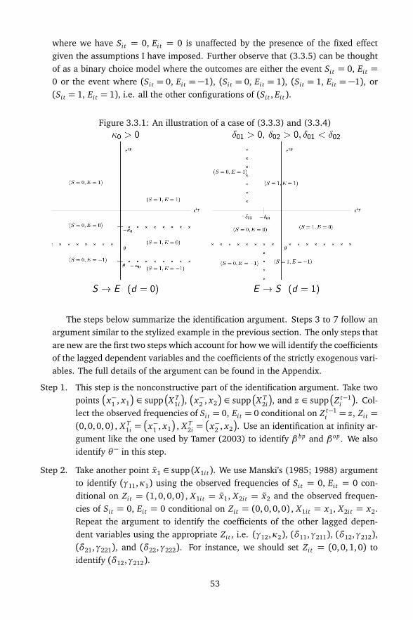
where we have Si t = 0, Ei t = 0 is unaffected by the presence of the fixed effectgiven the assumptions I have imposed. Further observe that (3.3.5) can be thoughtof as a binary choice model where the outcomes are either the event Si t = 0, Ei t =0 or the event where (Si t = 0, Ei t = −1), (Si t = 0, Ei t = 1), (Si t = 1, Ei t = −1), or(Si t = 1, Ei t = 1), i.e. all the other configurations of (Si t , Ei t).

Figure 3.3.1: An illustration of a case of (3.3.3) and (3.3.4)

The steps below summarize the identification argument. Steps 3 to 7 follow anargument similar to the stylized example in the previous section. The only steps thatare new are the first two steps which account for how we will identify the coefficientsof the lagged dependent variables and the coefficients of the strictly exogenous vari-ables. The full details of the argument can be found in the Appendix.

Step 1. This step is the nonconstructive part of the identification argument. Take twopoints

x−1 , x1

∈ supp

X T1i

,

x−2 , x2

∈ supp

X T2i

, and z ∈ supp

Z t−1i

. Col-lect the observed frequencies of Si t = 0, Ei t = 0 conditional on Z t−1

i = z, Zi t =(0,0, 0,0) , X T

1i =

x−1 , x1

, X T2i =

x−2 , x2

. Use an identification at infinity ar-gument like the one used by Tamer (2003) to identify β bp and β op. We alsoidentify θ− in this step.

Step 2. Take another point x1 ∈ supp (X1i t). We use Manski’s (1985; 1988) argumentto identify (γ11,κ1) using the observed frequencies of Si t = 0, Ei t = 0 con-ditional on Zi t = (1, 0,0, 0) , X1i t = x1, X2i t = x2 and the observed frequen-cies of Si t = 0, Ei t = 0 conditional on Zi t = (0, 0,0, 0) , X1i t = x1, X2i t = x2.Repeat the argument to identify the coefficients of the other lagged depen-dent variables using the appropriate Zi t , i.e. (γ12,κ2), (δ11,γ211), (δ12,γ212),(δ21,γ221), and (δ22,γ222). For instance, we should set Zi t = (0,0, 1,0) toidentify (δ12,γ212).

53

Step 3. Since (3.3.5) has the form of a fully parametric binary choice model as dis-cussed earlier, the copula dependence parameter ρ can be identified immedi-ately since the values of the parameters in Steps 1 and 2 are identified and canbe taken as known.

Step 4. The signs of δ01, δ02, and κ0 can now be identified.

Step 5. All the information from the previous steps can now be used to determinewhether di = 0 or di = 1.

Step 6. Since the groupings are now identified, we can recover the values of δ01, δ02,and κ0.

Steps 1 to 3 of the preceding argument can also be replaced by an alternative argu-ment where we exploit the form of (3.3.5). (3.3.5) is a fully parametric binary choicemodel and a likelihood function formed from pooling all the cross-sectional and timeseries information can be used to identify all the parameters mentioned in Steps 1 to3. This alternative avoids the rather nonconstructive nature of Step 1. Presenting theargument in these two ways is to set the stage for future work on weakening some ofthe parametric assumptions in Assumption A3. Furthermore, these two argumentsmay have different implications for estimation and inference. What I have shownis that point identification of all the common parameters is possible for (3.3.3) and(3.3.4).

3.3.3 Estimation and inference

Even though there would be incidental parameter bias when T is fixed and small,Hahn and Moon (2010) show that the incidental parameter bias disappears at amuch faster rate. Although the context they have in mind is estimating a game-theoretic model where the fixed effect represents the equilibrium chosen by players(when there are multiple equilibria), the idea that the fixed effect takes only a finitenumber of values applies to my proposal.

In particular, they show that, under certain regularity conditions, the reductionin support is automatically bias-reducing under an asymptotic scheme where n, T →∞ with n typically growing as an exponential function of T . Since the asymptoticdistribution of the MLE no longer has a noncentrality parameter (as opposed to theusual case where individual-specific effects are allowed to have full support overthe real line; see Hahn and Kuersteiner (2011)), inferences can be justified withoutresorting to bias-reduction procedures.

In this subsection, we impose the Gaussian copula for C and standard normalcumulative distribution functions for the margins Fεbp and Fεop in Assumption A3, justas in HI (2007). As a result, the dependence parameter ρ ∈ (−1, 1) coincides withthe usual correlation coefficient of the bivariate normal distribution. I still impose all

54

the assumptions required for identification here in this subsection. I use maximumlikelihood for estimation and inference. Collect all the common parameters into avector λ ∈ Λ and treat di ∈ 0,1 as a parameter to be estimated. As a result, thelog-likelihood for an arbitrary i and t is given by

li t (λ, di) =∑

j∈0,1

∑

k∈−1,0,1

1 (Si t = j, Ei t = k) log Pr

Si t = j, Ei t = k|Z ti , X T

1i , X T2i;λ, di

.

Aggregating over time for a fixed cross-sectional unit gives us the log-likelihood forthe ith cross-sectional unit:

li (λ, di) =T∑

t=1

li t (λ, di) .

Next, I impose the following additional assumptions:

E1 The parameters representing the simultaneous effects δ01, δ02, and κ0 cannot allbe jointly equal to zero.

E2 Let yi t =

Si t , Ei t , Si,t−1, Ei,t−1, Si,t−2, Ei,t−2, X1i t , X2i t

be the data for the ith unitand tth time period and di0 ∈ 0,1 be the true value of di . For each i,yi t : t = 1,2, . . . is strictly stationary. The differences of the joint distribu-tion of yi1, yi2, . . . across i is completely characterized by di0.

E3 Let

ε∗ = infi

G(i) (λ0, di0)− supdi 6=di0

G(i) (λ, di)

> 0,

whereG(i) (λ, d) = E(θ0,di0) [li (λ, d)] .

For all η > 0,

infi

G(i) (λ0, di0)− sup|λ−λ0|>η,d

G(i) (λ, d)

> 0.

The parameter space Λ is compact. There exists some M (yi t) such that

supλ,d

∂ k li t (λ, di)∂ λk

≤ M (yi t)

for k = 0,1 and maxi E [M (yi t)]2 <∞.

55

E4 Let ε > 0, η > 0 and θ be given. There exists some h (T ) strictly increasing in T ,such that, for all

di , d ′i

combinations, we have

Pr

1T

T∑

t=1

(li t (λ, di)−E [li t (λ, di)])

>η

3

= o

1h (T )

,

Pr

1T

T∑

t=1

(M (yi t)−E [M (yi t)])

>η

3ε

= o

1h (T )

,

where the probability and the expectation are calculated with respect to thedensity of (yi1, . . . , yiT ) indexed by

λ0, d ′i

.

Note that the individual-specific likelihood function under di = 0 becomes automati-cally distinguishable from the one under di = 1 provided that assumption E1 holds. Ifall these parameters representing simultaneous effects are jointly equal to zero, thereis no way to use time series variation to differentiate between di = 0 and di = 1. Thiscan be seen easily from Figure (3.3.1). Assumption E3 also holds because of the pre-vious statements along with the point-identification result in the previous subsection.The compactness ofΛ and the boundedness conditions on the likelihood and its scoreare standard regularity conditions imposed in maximum likelihood estimation. Notethat the log-likelihood I consider are continuously differentiable over the compact pa-rameter space. Furthermore, the parametric forms and time homogeneity assumedfor the model in (3.3.3) and (3.3.4) ensures that the data for every cross-sectionalunit are strictly stationary which satisfies Assumption E2. Finally, Assumption E4 is atechnical condition required to identify the correct group assignment. This assump-tion has been used in the literature on discrete parameter models (refer to Choiratand Seri (2012) and its references). Hahn and Moon (2010) and Choirat and Seri(2012) show that h (T ) is typically an exponential function of T .

Since Assumptions E2 to E4 are the same conditions used by Hahn and Moon(2010), adapting their Theorem 1 gives us:

Theorem 3.3.1. Let

Òdi (λ) = ar g max li (λ, di = 1) , li (λ, di = 0) ,

bλ = ar g maxλ

n∑

i=1

T∑

t=1

li t

λ,Òdi (λ)

,

eλ = ar g maxλ

n∑

i=1

T∑

t=1

li t (λ, di0) .

Suppose thatp

nT

eλ−λ d→ N (0,Σ) for some Σ. Under Assumptions E1 to E4, we

havep

nT

bλ−λ d→ N (0,Σ) if n→∞ and T →∞ such that n= O (h (T )).

56

The theorem states that the substitution of a plug-in Òdi (λ) for di is asymptoti-cally negligible. The covariance matrix Σ can either be the inverse of the Hessian orthe covariance matrix based on the sandwich formula. To estimate all the commonparameters, I use the following iterative approach:9

1. Set s = 0. Fix starting points for λ at λ(0).

2. Let li (λ, di) be the log-likelihood for the ith unit. If li

λ(s), 1

> li

λ(s), 0

,

then we set dd(s)i = 1. Otherwise, dd(s)i = 0.

3. Find the maximizer of∑

i li

λ(s),dd(s)i

and call it θ (s+1).

4. Set s to be s+ 1. Repeat Steps 2 and 3 until convergence.

Note that Step 2 corresponds to the profiling out of the fixed effects and that Step 3corresponds to finding the maximizer of the profile likelihood. The zigzag methodproposed is slightly slow in the application because I have to estimate around 54 to75 parameters. However, Step 2 is likely to be faster than the case where the fixedeffect could take on any value.

3.4 Revisiting the results of HI (1995; 2007)

3.4.1 Similarities and differences

Using PSID data10 from Waves 1 to 20, the authors estimate an econometric modelbased on the simultaneous determination of (Si t , Ei t) as seen in (3.3.1) and (3.3.2).They estimate both a binary probit and an ordered probit model where both indica-tors are jointly determined. Both their 1995 and 2007 papers impose the coherencyconditions κ0 = 0 or δ01 = δ02 = 0. Therefore, they will have two sets of results –a set of results based on δ01 = δ02 = 0 and another based on κ0 = 0. In contrast, Ijointly estimate (3.3.3) and (3.3.4) without imposing the coherency conditions.

They incorporate dynamic effects in the model by introducing lagged values ofthe corresponding indicators. The other regressors are variables that represent char-acteristics of the household head and the labor market to which the household headwas exposed. The list of regressors used in both the 1995 and 2007 papers can befound in Table 3.6.2 found in the Appendix. I exclude the cube of age in the list ofregressors because the resulting Hessian was singular.11 The 1995 paper makes useof exclusion restrictions when estimating (3.3.1) and (3.3.2). On the other hand,

9The algorithm is not exactly an application of the EM algorithm. The fixed effects di I introduce intothe model are not just labels. The values that di take have a direct interpretation.

10I use data made available by the authors in the Journal of Applied Econometrics data archive.11Freedman and Sekhon (2010) document some of the numerical issues involved in estimating systems

of equations with discrete endogenous variables even with very few regressors.

57

the 2007 paper does not have any exclusion restrictions at all. For instance, the ageof the household head may influence both Si t and Ei t , but being a union membermay influence Ei t but not Si t . Meango and Mourifie (2013) show that some pa-rameters are only partially identified in two-equation probit models with a dummyendogenous regressor when there are no exclusion restrictions. In contrast, I applythe exclusion restrictions in HI (1995).12

In addition to (3.3.1) and (3.3.2), they assume that the error terms

εbpi t ,εop

i t

have an AR(1) structure:

εbpi t = η

bpi + ς

bpi t , ςbp

i t = ρbpς

bpi,t−1 + ξ

bpi t ,

ρbp

< 1, (3.4.1)

εopi t = η

opi + ς

opi t , ςop

i t = ρopς

opi,t−1 + ξ

opi t , |ρop|< 1, (3.4.2)

where

ηbpi ,ηop

i

represent time-invariant unobserved heterogeneity and

ξbpi t ,ξop

i t

are both i.i.d. Gaussian random variables with mean zero, variance 1 and havenonzero correlationρ conditional on the strictly exogenous regressors X i = (X i1, . . . , X iT ).They use the Mundlak-Chamberlain device to model

ηbpi ,ηop

i

. In particular, they

assume thatηbpi |X i ∼ N

X i.θbp,σ2

bp

andηopi |X i ∼ N

X i.θop,σ2

op

. They also modelthe initial conditions using an analogous assumption. In contrast, I use di to repre-sent time-invariant unobserved heterogeneity that may be arbitrarily correlated withX i . All my results are conditional on the initial observation. I allowed for a similarAR(1) structure but results were not forthcoming as will be discussed below.

Strictly speaking, the model I consider neither encompasses nor generalizes themodel that HI (1995; 2007) consider. HI (1995; 2007) use large-n, fixed-T asymp-totics to justify their results. In contrast, I use large-n, large-T asymptotics to justifymy results. Introducing additive fixed effects and modelling these effects using theMundlak-Chamberlain device may require substantial changes to the identificationargument and the justification of the estimation procedure. Even without resortingto the Mundlak-Chamberlain device, it is not clear how to justify existing bias reduc-tion procedures meant for panel data models with fixed effects that have full support.Despite these concerns, the results I present point to the conclusion that imposingcoherency conditions may be inappropriate.

3.4.2 Results

There are a total of 32408 observations on 2410 male household heads observedfor an average number of 14 periods. Complete spells accounted for 528 out of the2410 male household heads. I exclude all household heads with spells of length 1 in

12Nevertheless, I estimate the model without the exclusion restrictions because recent work by Hanand Vytlacil (2015) point to the possibility of point identification even if there are common exogenousregressors and there are no exclusion restrictions. For now, the identification argument in Section 3.3require exclusion restrictions. The regressors with large support in the binary choice equation that HI(1995; 2007) use are food needs (fneed) and the growth of food needs (gfneed).

58

the analysis. Table 3.6.1 in the Appendix has the distribution of spell length for thehousehold heads in the sample.

I compute all the results in this section using R (R Core Team, 2014). I usethe optimx package, the accompanying BFGS algorithm, and the programmed testsfor the Karush-Kuhn-Tucker optimality conditions (see Nash and Varadhan (2011)and Nash (2014) for more details). All results presented below have passed thesetests. I use estimates found in HI (1995; 2007) as possible starting points for thealgorithm.13

Given the discussion in the previous subsection, I estimate 3 different specifica-tions:

1. Specification A uses the list of regressors in HI (1995) but only allows for ownstate dependence, i.e. δ11 = δ12 = δ21 = δ22 = 0 in (3.3.3) and κ1 = κ2 = 0in (3.3.4). There are 56 parameters to be estimated in this case.

2. Specification B uses the list of regressors in HI (1995) but removes the restric-tions just mentioned. As a result, I account for some form of spillover effect.There are 62 parameters to be estimated in this case.

3. Specification C uses the same set of regressors in both (3.3.3) and (3.3.4). Therestrictions just mentioned are also removed. There are 73 parameters to beestimated in this case.

Furthermore, I consider two samples – Sample 1 consists of observations from Waves1 to 14 while Sample 2 consists of observations from Waves 1 to 20. We presentthe coefficient estimate and their corresponding standard errors immediately below.Coefficients that are statistically significant at the 1% level are in bold.

Table 3.4.1: Main Results

Specification A Specification B Specification CSample 1 Sample 2 Sample 1 Sample 2 Sample 1 Sample 2

δ01 0.693 0.293 0.489 0.283 0.489 0.309(0.084) (0.057) (0.078) (0.058) (0.078) (0.058)

δ02 0.042 −0.402 −0.721 −0.612 −0.770 −0.601(0.053) (0.036) (0.054) (0.041) (0.055) (0.040)

κ0 1.326 1.128 1.429 1.282 1.413 1.281(0.034) (0.025) (0.036) (0.028) (0.036) (0.028)

θ− −5.697 −5.645 −5.714 −5.668 −5.719 −5.680(0.008) (0.007) (0.008) (0.007) (0.008) (0.007)

ρ −0.007 0.001 0.000 −0.001 0.001 −0.000(0.005) (0.004) (0.004) (0.004) (0.005) (0.004)

13These starting points are based on Tables 8 and 9 of HI (1995) and Tables VI and VII of HI (2007). Ifind that the results are not sensitive to these starting points.

59

I impose the AR(1) error structure used by the authors. However, the estimatedfirst-order autocorrelation coefficients are extremely small (with sizes around 10−6).14

In contrast, the authors found first-order autocorrelation coefficients around therange of 0.40 to 0.68 and are significantly different from zero. Therefore, I set asidethe AR(1) structure for the rest of the calculations.

The results in Table 3.4.1 indicate that imposing the coherency condition may notbe appropriate. Note that δ01, δ02, and κ0 are significantly different from zero acrossall specifications and samples (except for the one found in Specification A, Sample1). Furthermore, the signs are very different from their results. For instance, theimmediate effect of being involuntarily unemployed/underemployed on the proba-bility of being liquidity constrained is negative while they estimate it as positive. Theabsolute values of the coefficients are much larger compared to the results by the au-thors. For instance, their estimates of κ0 range from 0.12 to 0.13. There are somedifferences in the estimates for δ01 and δ02 in Specification A relative to the otherspecifications because Specification A does not include lagged spillover effects. Theremight also be indications of parameter nonconstancy as one moves from Sample 1to Sample 2. Nevertheless, the results are qualitatively unchanged.

Table 3.4.2: Results on the effects of state dependence for Specification A

Equation for Si t Equation for Ei tSample 1 Sample 2 Sample 1 Sample 2

Si,t−1 1.512 1.535(0.031) (0.025)

Si,t−2 0.313 0.459(0.031) (0.025)

1

Ei,t−1 = −1

−1.868 −1.885(0.051) (0.040)

1

Ei,t−2 = −1

−0.811 −0.883(0.053) (0.042)

1

Ei,t−1 = 1

0.923 0.983(0.028) (0.021)

1

Ei,t−2 = 1

0.523 0.539(0.028) (0.022)

It is clear from Table 3.4.1 that the coherency conditions imposed by HI (1995;2007) are unlikely to be true for all household heads. The estimated lower thresholdassociated with involuntary unemployment/underemployment relative to voluntaryis twice the value estimated by the authors. This means that the lower thresholdis not as tight as HI (1995; 2007) estimate. The estimated correlation ρ between

14Even with different starting values, as noted in the preceding footnote, the estimates for the first-orderautocorrelation coefficients are also very near zero.

60

the error terms

εbpi t ,εop

i t

is not significantly different from zero, while the authorsestimate this correlation at around 0.34 to 0.43 and are significantly different fromzero. It is may be possible that the nonzero correlation of the error terms estimatedby HI (1995; 2007) is an artifact of imposing the coherency conditions.

The results in Tables 3.4.2, 3.4.3, and 3.4.4 indicate that there are statisticallysignificant effects of state dependence. In particular, the existence of own state de-pendence is a major feature common to the three tables. As a result, householdheads that were liquidity constrained in the previous periods are more likely to beliquidity constrained now. I find a similar result for employment status. In particular,household heads who were overemployed in previous periods are more likely to beoveremployed now.

Tables 3.4.3 and 3.4.4 indicate the possibility of lagged spillover effects, espe-cially for employment status.15 In particular, household heads that were liquidityconstrained in previous periods are more likely to be overemployed now. The resultsalso indicate that past employment status (except for household heads who wereinvoluntarily unemployed/underemployed one period ago) may not be a significantindicator for determining whether household heads are more or less likely to beliquidity constrained now. Since being liquidity constrained or being involuntarilyoveremployed or unemployed for two periods in the past still has a significant effecton the current state of the household head, even after controlling for contemporane-ous effects, the results paint quite a negative picture of the lasting effects of liquidityand employment constraints.

Table 3.4.3: Results on the effects of state dependence for Specification B

Equation for Si t Equation for Ei tSample 1 Sample 2 Sample 1 Sample 2

Si,t−1 1.496 1.519 −0.385 −0.385(0.031) (0.025) (0.038) (0.030)

Si,t−2 0.297 0.444 −0.128 −0.115(0.031) (0.025) (0.035) (0.028)

1

Ei,t−1 = −1

−0.018 −0.013 −1.856 −1.876(0.059) (0.046) (0.051) (0.040)

1

Ei,t−2 = −1

−0.097 −0.042 −0.821 −0.882(0.058) (0.046) (0.053) (0.042)

1

Ei,t−1 = 1

0.124 0.123 0.941 1.008(0.032) (0.025) (0.028) (0.021)

1

Ei,t−2 = 1

0.046 0.059 0.529 0.561(0.032) (0.025) (0.029) (0.022)

15Note that these lagged spillover effects do not exactly represent the absence of Granger non-causalitysince the model includes contemporaneous terms.

61

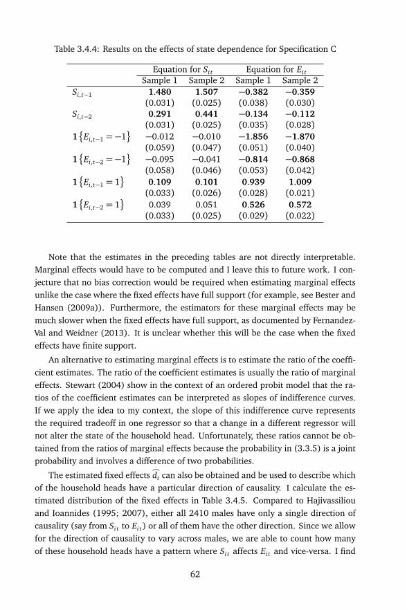
Table 3.4.4: Results on the effects of state dependence for Specification C

Equation for Si t Equation for Ei tSample 1 Sample 2 Sample 1 Sample 2

Si,t−1 1.480 1.507 −0.382 −0.359(0.031) (0.025) (0.038) (0.030)

Si,t−2 0.291 0.441 −0.134 −0.112(0.031) (0.025) (0.035) (0.028)

1

Ei,t−1 = −1

−0.012 −0.010 −1.856 −1.870(0.059) (0.047) (0.051) (0.040)

1

Ei,t−2 = −1

−0.095 −0.041 −0.814 −0.868(0.058) (0.046) (0.053) (0.042)

1

Ei,t−1 = 1

0.109 0.101 0.939 1.009(0.033) (0.026) (0.028) (0.021)

1

Ei,t−2 = 1

0.039 0.051 0.526 0.572(0.033) (0.025) (0.029) (0.022)

Note that the estimates in the preceding tables are not directly interpretable.Marginal effects would have to be computed and I leave this to future work. I con-jecture that no bias correction would be required when estimating marginal effectsunlike the case where the fixed effects have full support (for example, see Bester andHansen (2009a)). Furthermore, the estimators for these marginal effects may bemuch slower when the fixed effects have full support, as documented by Fernandez-Val and Weidner (2013). It is unclear whether this will be the case when the fixedeffects have finite support.

An alternative to estimating marginal effects is to estimate the ratio of the coeffi-cient estimates. The ratio of the coefficient estimates is usually the ratio of marginaleffects. Stewart (2004) show in the context of an ordered probit model that the ra-tios of the coefficient estimates can be interpreted as slopes of indifference curves.If we apply the idea to my context, the slope of this indifference curve representsthe required tradeoff in one regressor so that a change in a different regressor willnot alter the state of the household head. Unfortunately, these ratios cannot be ob-tained from the ratios of marginal effects because the probability in (3.3.5) is a jointprobability and involves a difference of two probabilities.

The estimated fixed effects Òdi can also be obtained and be used to describe whichof the household heads have a particular direction of causality. I calculate the es-timated distribution of the fixed effects in Table 3.4.5. Compared to Hajivassiliouand Ioannides (1995; 2007), either all 2410 males have only a single direction ofcausality (say from Si t to Ei t) or all of them have the other direction. Since we allowfor the direction of causality to vary across males, we are able to count how manyof these household heads have a pattern where Si t affects Ei t and vice-versa. I find

62

that around half of the 2410 males have a pattern where Si t affects Ei t across spec-ifications and across different samples. I also find that some of these males changepatterns from Sample 1 to Sample 2. In particular, around 12% of the males fromSample 1 change patterns once we observed them for more time periods.

Table 3.4.5: Estimated distribution of the fixed effects Òdi

Specification A Specification B Specification CSample 1 Sample 2 Sample 1 Sample 2 Sample 1 Sample 2

Si t → Ei t 1101 1214 1100 1221 1103 1209Ei t → Si t 1001 1186 1002 1179 999 1191Total 2102 2400 2102 2400 2102 2400

Finally, the tables in the appendix contain results for the coefficients of the strictlyexogenous regressors across different specifications and samples. Apart from a fewcoefficients changing signs across specifications and samples (in particular, house-hold age and some of the dummies representing residence, ethnicity, and religion),the results are quite similar to one another and are consistent with expectations.However, most of the positive coefficients in Sample 1 are larger than those in Sam-ple 2. Similarly, most of the negative coefficients in Sample 1 are larger in absolutevalue than those in Sample 2.

3.5 Concluding remarks

In this chapter, I have developed a route toward identification, estimation, and infer-ence in dynamic simultaneous equations models with discrete outcomes when paneldata is available. These models are subject to the incidental parameter problem whenindividual-specific fixed effects are included and are also subject to incoherence andincompleteness. I introduce a specific type of individual-specific fixed effect so thatthe coherency condition need not be imposed across all observations. This proposalallows us to avoid imposing sign restrictions or to avoid restricting error supports.

Specifically, I use a subset of the observables unaffected by the individual-specificfixed effect to identify the common parameters of the model. I then use time seriesvariation to identify the individual-specific fixed effect. This fixed effect representsthe direction of causality from one endogenous variable to another. Knowing the di-rection allows us to identify the coefficients of the endogenous variables. Consistentestimation and correct inference without any need for bias reduction follows fromthe large-n, large-T asymptotic theory. I revisit the empirical application of Hajivas-siliou and Ioannides (1995; 2007) and find strikingly different results with respect to

63

the contemporaneous interaction and dynamic structure of employment status andliquidity constraints.

Future work may consider the computation of certain types of marginal effectsdefined in Lewbel, Dong, and Yang (2012). Future work in this area may also al-low the specification of individual-specific effects to be time-varying as well, just asBonhomme and Manresa (2015) do for groupings in the linear model. There seemsto be some slight evidence in the empirical application that cast some doubt on theassumption that the direction of causality is time-invariant. However, it may well bethe case that we have restricted time-invariant unobserved heterogeneity too much.Introducing another fixed effect in the linear predictor may be fruitful but is beyondthe scope of this chapter. Although the approach would seem fruitful, bias-reductionprocedures have to be adapted for the case I considered. A natural alternative wouldbe to use each cross-section to set-identify the parameters of the model (as seen inSection 2) and find methods to combine these set estimates across different timeperiods.

3.6 Appendix

Details of identification argument in Section 3.3.2

Let us now examine the details behind each step of the identification argument. InStep 1, we need to calculate the probability that Si t = 0 and Ei t = 0 conditional onZi t = (0,0, 0,0) , X T

1i =

x−1 , x1

, X T2i =

x−2 , x2

:

Pr

S∗i t ≤ 0,θ− ≤ E∗i t ≤ 0|Z t−1i = z, Zi t = (0,0, 0,0) , X T

1i =

x−1 , x1

, X T2i =

x−2 , x2

A2= Pr

S∗i t ≤ 0,θ− ≤ E∗i t ≤ 0|Zi t = (0, 0,0, 0) , X1i t = x1, X2i t = x2

A1= Pr

εbpi t ≤ −x1β

bp,θ− − x2βop ≤ εop

i t ≤ −x2βop

Let

β bp, β op

be such that

β bp,β op

6=

β bp, β op

. Without loss of generality, let x1k

be the kth regressor in x1 and β bpk , β bp

k > 0 be the associated coefficient of this regres-sor. As x1k → −∞ given the other regressors in x1, we have −x1kβ

bpk , −x1kβ

bpk →

∞. Since x2 has full rank by A5, we have x2 such that x2βop 6= x2β

op. We now have

Pr

εbpi t ≤ −x1β

bp,θ− − x2βop ≤ εop

i t ≤ −x2βop

≈ Pr

θ− − x2βop ≤ εop

i t ≤ −x2βop

6= Pr

θ− − x2βop ≤ εop

i t ≤ −x2βop

≈ Pr

εbpi t ≤ −x1β

bp,θ− − x2βop ≤ εop

i t ≤ −x2βop

.

64

As a result, β op is identified. Since x1 has full rank by A5, we have x1 such thatx1β

bp 6= x1βbp. Following the same argument as before, we have

Pr

εbpi t ≤ −x1β

bp,θ− − x2βop ≤ εop

i t ≤ −x2βop

6= Pr

εbpi t ≤ −x1β

bp,θ− − x2βop ≤ εop

i t ≤ −x2βop

.

As a result, β bp is identified. For the case where β bpk < 0, we have −x1kβ

bpk →∞

but −x1kβbpk →−∞. Following the same argument as before, we can identify both

β bp and β op. Note that the constant terms in β bp and β op are also identified.

Now, we identify θ−. Without loss of generality, let θ− < θ− < 0. Since β bp andβ op are both identified, we take them as fixed in this step. Recall that we have

Pr

εbpi t ≤ −x1β

bp,θ− − x2βop ≤ εop

i t ≤ −x2βop

6= Pr

εbpi t ≤ −x1β

bp, θ− − x2βop ≤ εop

i t ≤ −x2βop

.

As a result, θ− is identified.

Step 2 uses Manski’s (1985; 1988) identification argument to identify the co-efficients of the lagged dependent variables. To illustrate, consider the followingprobabilities:

Pr

Si t = 0, Ei t = 0|Z t−1i = z, Zi t = (0,0, 0,0) , X T

1i =

x−1 , x1

, X T2i =

x−2 , x2

= Pr

εbpi t ≤ −x1β

bp,θ− − x2βop ≤ εop

i t ≤ −x2βop

, (3.6.1)

and

Pr

Si t = 0, Ei t = 0|Z t−1i = z, Zi t = (1,0, 0,0) , X T

1i =

x−1 ,fx1

, X T2i =

x−2 ,fx2

= Pr

εbpi t ≤ − x1β

bp − γ11,θ− − x2βop − κ1 ≤ ε

opi t ≤ − x2β

op −κ1

. (3.6.2)

The expressions (3.6.1) and (3.6.2) will only be equal if and only if

−x1βbp = −fx1β

bp − γ11,

−x2βop = −fx2β

op − κ1.

Therefore, both γ11 and κ1 are identified because γ11 = (x1 −fx1)β bp and κ1 =(x2 −fx2)β op under the support condition in assumption A5. Similar arguments canbe used to identify the coefficients of the other lagged dependent variables.

Step 3 follows from recognizing that we have a fully parametric binary choicemodel in (3.3.5) with only one copula dependence parameter left to identify.

65

In Step 4, we identify the signs of δ01, δ02, and κ0. Note that we have

Pr

Si t = 0, Ei t = −1|Z t−1i = z, Zi t = (0, 0,0, 0) , X T

1i =

x−1 , x1

, X T2i =

x−2 , x2

=Pr

εbpi t ≤ −x1β

bp −δ01,εopi t ≤ θ

− − x2βop

Pr (di = 1)

+ Pr

εbpi t ≤ −x1β

bp,εopi t ≤ θ

− − x2βop

Pr (di = 0) .

Showing that this conditional probability is greater than

Pr

εbpi t ≤ −x1β

bp,εopi t ≤ θ

− − x2βop

allows us to conclude that δ01 < 0. The other cases follow analogously. Note that toavoid cumbersome notation, I omit the conditioning set in Pr (di = 1) and Pr (di = 0).

For Step 5, there are eight cases to consider. The resulting group assignmentrules follows the same intuition as Table 3.2.1 and by sketching figures like Figure(3.3.1). One of the cases is that once we know that δ01 > 0, δ02 > 0, and κ0 > 0,we must assign di = 0 if and only if

Pr

Ei t = 0|Z t−1i = z, Zi t = (0, 0,0, 0) , X T

1i =

x−1 , x1

, X T2i =

x−2 , x2

> Pr

εopi t ≥ −x2β

op

or assign di = 1 if and only if

Pr

Si t = 0|Z t−1i = z, Zi t = (0, 0,0, 0) , X T

1i =

x−1 , x1

, X T2i =

x−2 , x2

> Pr

εbpi t ≤ −x1β

bp

Of course, these assignment rules can be altered by changing the conditioning sets.The other cases follow similarly.

In Step 6, we can now point-identify δ01, δ02, and κ0. One route is to look at theconditional probability of (Si t = 1, Ei t = 1) given Z t−1

i = z, Zi t = (0,0, 0,0) , X T1i =

x−1 , x1

, X T2i =

x−2 , x2

, di = 0. This conditional probability is now a function of κ0

and can be used to point-identify κ0. The conditional probability of (Si t = 0, Ei t = −1)given Z t−1

i = z, Zi t = (0,0, 0,0) , X T1i =

x−1 , x1

, X T2i =

x−2 , x2

, di = 1 can be usedto point-identify δ01. Finally, the conditional probability of (Si t = 0, Ei t = 1) givenZ t−1

i = z, Zi t = (0,0, 0,0) , X T1i =

x−1 , x1

, X T2i =

x−2 , x2

, di = 1 can be used topoint-identify δ02. Alternative routes include changing the vector Zi t or using otherregions found in Figure 3.3.1.

66

Empirical Results

There are five tables in this Appendix. Table 3.6.1 contain the distribution of spelllengths in the data. Table 3.6.2 contains a description of the regressors used in theempirical application. Tables 3.6.3, 3.6.4, and 3.6.5 contain the estimation resultsfor Specifications A, B, and C, respectively, across Samples 1 and 2.

Table 3.6.1: Length of spells observed in the data

Number of periods 1 2 3 4 5 6 7 8 9 10Number of males 10 13 23 30 130 131 93 132 121 116Number of periods 11 12 13 14 15 16 17 18 19 20Number of males 103 121 138 124 124 118 125 127 103 528

67

Table3.6.2:

Listof

variablesin

Hajivassiliou

andIoannides

(1995)

Modelfor

Regressors

inX

itS

iteducationalcategory

ofhead

(edycat)dum

mies

for1976-79

and1980-83

periods(era7679,era8083)

foodneeds,grow

thof

foodneeds

(fneed,gfneed)age,age

squared,agecubed

(hage)live

innorth/central,south,w

est,otherregions

(liveinnc,liveinso,liveinwe,liveinot)m

arried,raceis

blackor

other(msm,raceb,raceo)

religionis

Christian,Jew

ish,orProtestant

(religceo,religjsh,religpro)realrate

ofinterest

(rri)E

itcounty

unemploym

entrate

(cunemp)head

disabled,educationalcategoryof

head(disab,edycat)

dumm

iesfor

1976-79and

1980-83periods

(era7679,era8083)food

needs,growth

offood

needs(fneed,gfneed)

age,agesquared,age

cubed(hage)

tenure,tenuresquared

(htenure)unem

ployment

insurancereceived

byhead

(hunemins)im

putedw

age(impwage) a

tightnessof

laborm

arketconditions

(labmkt)

livein

north/central,south,west,other

regions(liveinnc,liveinso,liveinwe,liveinot)

married,num

berof

childrenbetw

een0-5

(msm,numch05)occupationalunem

ployment

rate(occunemp)

raceis

blackor

other(raceb,raceo)

religionis

Christian,Jew

ish,orProtestant

(religceo,religjsh,religpro)realrate

ofinterest

(rri)head

isunion

mem

ber(unionmem)

aTheauthors

includea

variablerepresenting

some

measure

ofthe

imputed

wage

(impwage).U

nfortunately,theJA

Edata

archivedid

notinclude

thisvariable.

68

Tabl

e3.

6.3:

Res

ults

for

Spec

ifica

tion

A

Sam

ple

1Sa

mpl

e2

Equa

tion

for

S it

Equa

tion

for

E it

Equa

tion

for

S it

Equa

tion

for

E it

Vari

able

Coe

fSE

Vari

able

Coe

fSE

Vari

able

Coe

fSE

Vari

able

Coe

fSE

Reg

ress

ors

com

mon

tobo

theq

uati

ons

Inte

rcep

t1.

270

0.15

1In

terc

ept

-2.3

660.

166

Inte

rcep

t0.

939

0.12

2In

terc

ept

-1.5

720.

129

era7

679

0.14

10.

033

era7

679

0.00

20.

035

era7

679

0.13

40.

030

era7

679

0.03

50.

030

era8

083

-0.3

110.

054

era8

083

-0.4

600.

054

era8

083

-0.0

910.

031

era8

083

0.09

90.

030

edyc

at-0

.043

0.00

8ed

ycat

-0.0

270.

008

edyc

at-0

.054

0.00

6ed

ycat

-0.0

710.

006

hage

-11.

077

0.77

5ha

ge1.

925

0.72

1ha

ge-9

.399

0.61

6ha

ge-1

.118

0.55

2ha

gesq

9.20

70.

944

hage

sq-4

.754

0.87

2ha

gesq

7.22

10.

746

hage

sq-0

.471

0.66

0li

vein

nc-0

.071

0.03

7li

vein

nc-0

.086

0.03

6li

vein

nc-0

.068

0.03

0li

vein

nc-0

.108

0.02

8li

vein

ot0.

502

0.15

1li

vein

ot0.

228

0.16

1li

vein

ot0.

365

0.10

9li

vein

ot0.

123

0.11

1li

vein

so0.

073

0.03

8li

vein

so0.

123

0.03

9li

vein

so0.

064

0.03

0li

vein

so-0

.046

0.02

9li

vein

we0.

018

0.04

3li

vein

we-0

.436

0.04

2li

vein

we0.

050

0.03

3li

vein

we-0

.400

0.03

3ms

s0.

577

0.04

3ms

s-0

.209

0.04

2ms

s0.

547

0.03

4ms

s-0

.214

0.03

1ra

ceb

0.38

00.

056

race

b0.

208

0.05

1ra

ceb

0.39

00.

045

race

b0.

275

0.04

0ra

ceo

-0.3

720.

054

race

o0.

140

0.04

9ra

ceo

-0.3

470.

049

race

o0.

222

0.04

3re

ligc

eo0.

092

0.04

4re

ligc

eo0.

273

0.04

2re

ligc

eo0.

125

0.03

4re

ligc

eo0.

235

0.03

2re

ligj

sh0.

201

0.08

1re

ligj

sh0.

198

0.08

1re

ligj

sh0.

197

0.06

9re

ligj

sh0.

165

0.06

7re

ligp

ro0.

060

0.03

3re

ligp

ro0.

006

0.03

3re

ligp

ro0.

157

0.02

5re

ligp

ro0.

070

0.02

5rr

i10

.017

1.11

5rr

i13

.997

1.14

1rr

i6.

891

0.61

6rr

i4.

193

0.63

2R

egre

ssor

sth

atar

ein

clud

edin

one

ofth

eeq

uati

ons

but

excl

uded

inth

eot

her

fnee

d0.

254

0.37

4cu

nemp

0.87

40.

596

fnee

d0.

306

0.31

7cu

nemp

0.67

90.

391

gfne

ed-0

.400

0.04

7di

sab

0.27

00.

044

gfne

ed-0

.508

0.03

9di

sab

0.13

60.

034

hten

ure

-3.5

420.

412

hten

ure

-3.9

380.

325

hten

ursq

8.65

01.

519

hten

ursq

8.05

11.

183

hune

mins

0.55

70.

032

hune

mins

0.35

40.

016

labm

kt0.

032

0.01

4la

bmkt

0.05

50.

011

numc

h05

0.00

70.

022

numc

h05

0.01

80.

016

occu

nemp

5.86

50.

518

occu

nemp

3.64

70.

319

unio

nmem

0.21

50.

029

unio

nmem

0.21

30.

023

69

Table3.6.4:

Results

forSpecification

B

Sample

1Sam

ple2

Equationfor

Sit

Equationfor

Eit

Equationfor

Sit

Equationfor

Eit

VariableC

oefSE

VariableC

oefSE

VariableC

oefSE

VariableC

oefSE

Regressors

comm

onto

bothequations

Intercept1.347

0.153Intercept

-2.1060.169

Intercept0.896

0.123Intercept

-1.3910.131

era76790.141

0.033era7679

0.0110.034

era76790.124

0.030era7679

0.0380.030

era8083-0.320

0.054era8083

-0.4540.054

era8083-0.081

0.031era8083

0.0880.030

edycat-0.047

0.008edycat

-0.0340.008

edycat-0.050

0.006edycat

-0.0740.006

hage-11.074

0.781hage

1.1500.725

hage-9.344

0.618hage

-1.3480.556

hagesq9.133

0.950hagesq

-4.1310.873

hagesq7.227

0.748hagesq

-0.5020.663

liveinnc-0.068

0.037liveinnc

-0.0480.036

liveinnc-0.065

0.030liveinnc

-0.1110.028

liveinot0.505

0.153liveinot

0.3270.162

liveinot0.388

0.109liveinot

0.1380.112

liveinso0.074

0.038liveinso

0.1280.039

liveinso0.069

0.030liveinso

-0.0360.029

liveinwe0.012

0.043liveinwe

-0.4010.042

liveinwe0.055

0.034liveinwe

-0.3900.032

mss0.569

0.044mss

-0.1460.042

mss0.542

0.034mss

-0.1850.031

raceb0.405

0.057raceb

0.2130.052

raceb0.381

0.045raceb

0.2800.040

raceo-0.399

0.055raceo

0.1540.050

raceo-0.355

0.049raceo

0.2190.043

religceo0.097

0.044religceo

0.2470.042

religceo0.131

0.034religceo

0.2350.032

religjsh0.209

0.081religjsh

0.1740.082

religjsh0.199

0.070religjsh

0.1370.067

religpro0.053

0.034religpro

-0.0270.033

religpro0.160

0.025religpro

0.0610.025

rri10.481

1.125rri

13.6721.137

rri6.476

0.622rri

4.2470.632

Regressors

thatare

includedin

oneof

theequations

butexcluded

inthe

otherfneed

0.1010.379

cunemp1.233

0.597fneed

0.1890.319

cunemp0.338

0.391gfneed

-0.3950.048

disab0.280

0.044gfneed

-0.5120.039

disab0.135

0.034htenure

-3.6950.413

htenure-4.087

0.329htenursq

9.0441.528

htenursq8.060

1.208hunemins

0.5370.032

hunemins0.356

0.016labmkt

0.0370.014

labmkt0.060

0.010numch05

0.0130.022

numch050.019

0.016occunemp

5.8890.519

occunemp3.717

0.318unionmem

0.1840.029

unionmem0.204

0.023

70

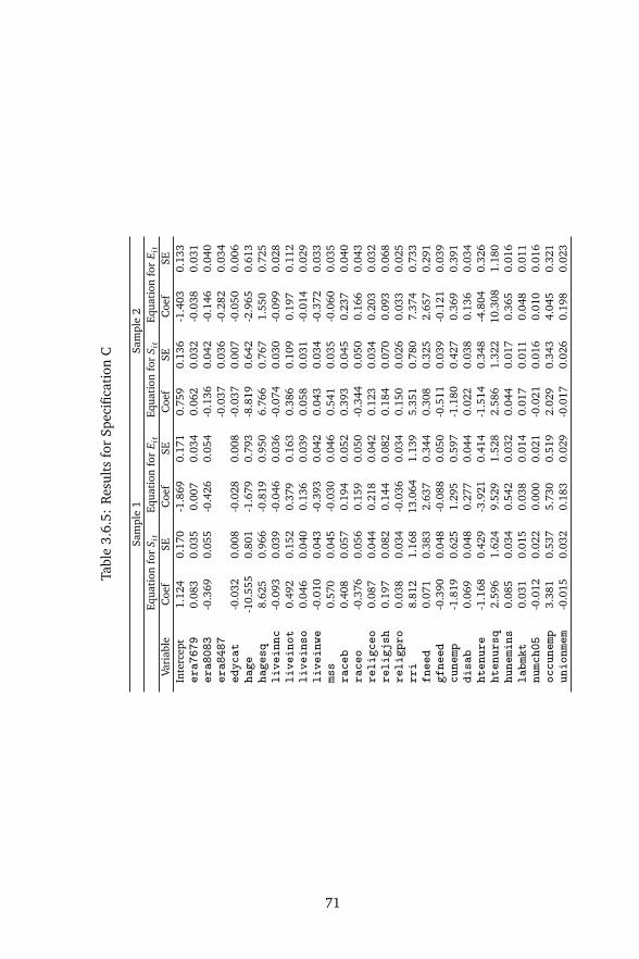
Tabl

e3.

6.5:

Res

ults

for

Spec

ifica

tion

C

Sam

ple

1Sa

mpl

e2

Equa

tion

for

S it

Equa

tion

for

E it

Equa

tion

for

S it

Equa

tion

for

E it

Vari

able

Coe

fSE

Coe

fSE

Coe

fSE

Coe

fSE

Inte

rcep

t1.

124

0.17

0-1

.869

0.17

10.

759

0.13

6-1

.403

0.13

3er

a767

90.

083

0.03

50.

007

0.03

40.

062

0.03

2-0

.038

0.03

1er

a808

3-0

.369

0.05

5-0

.426

0.05

4-0

.136

0.04

2-0

.146

0.04

0er

a848

7-0

.037

0.03

6-0

.282

0.03

4ed

ycat

-0.0

320.

008

-0.0

280.

008

-0.0

370.

007

-0.0

500.

006

hage

-10.

555

0.80

1-1

.679

0.79

3-8

.819

0.64

2-2

.965

0.61

3ha

gesq

8.62

50.

966

-0.8

190.

950

6.76

60.

767

1.55

00.

725

live

innc

-0.0

930.

039

-0.0

460.

036

-0.0

740.

030

-0.0

990.

028

live

inot

0.49

20.

152

0.37

90.

163

0.38

60.

109

0.19

70.

112

live

inso

0.04

60.

040

0.13

60.

039

0.05

80.

031

-0.0

140.

029

live

inwe

-0.0

100.

043

-0.3

930.

042

0.04

30.

034

-0.3

720.

033

mss

0.57

00.

045

-0.0

300.

046

0.54

10.

035

-0.0

600.

035

race

b0.

408

0.05

70.

194

0.05

20.

393

0.04

50.

237

0.04

0ra

ceo

-0.3

760.

056

0.15

90.

050

-0.3

440.

050

0.16

60.

043

reli

gceo

0.08

70.

044

0.21

80.

042

0.12

30.

034

0.20

30.

032

reli

gjsh

0.19

70.

082

0.14

40.

082

0.18

40.

070

0.09

30.

068

reli

gpro

0.03

80.

034

-0.0

360.

034

0.15

00.

026

0.03

30.

025

rri

8.81

21.

168

13.0

641.

139

5.35

10.

780

7.37

40.

733

fnee

d0.

071

0.38

32.

637

0.34

40.

308

0.32

52.

657

0.29

1gf

need

-0.3

900.

048

-0.0

880.

050

-0.5

110.

039

-0.1

210.

039

cune

mp-1

.819

0.62

51.

295

0.59

7-1

.180

0.42

70.

369

0.39

1di

sab

0.06

90.

048

0.27

70.

044

0.02

20.

038

0.13

60.

034

hten

ure

-1.1

680.

429

-3.9

210.

414

-1.5

140.

348

-4.8

040.

326

hten

ursq

2.59

61.

624

9.52

91.

528

2.58

61.

322

10.3

081.

180

hune

mins

0.08

50.

034

0.54

20.

032

0.04

40.

017

0.36

50.

016

labm

kt0.

031

0.01

50.

038

0.01

40.

017

0.01

10.

048

0.01

1nu

mch0

5-0

.012

0.02

20.

000

0.02

1-0

.021

0.01

60.

010

0.01

6oc

cune

mp3.

381

0.53

75.

730

0.51

92.

029

0.34

34.

045

0.32

1un

ionm

em-0

.015

0.03

20.

183

0.02

9-0

.017

0.02

60.

198

0.02

3

71

72

Chapter 4

Estimation and inference indynamic nonlinear fixed effectspanel data models byprojection

4.1 Introduction

Neyman and Scott (1948) show that the method of maximum likelihood may fail toproduce consistent and asymptotically efficient estimators when there are incidentalparameters. Lancaster (2000) documents some of the developments after the publi-cation of their paper. Roughly, these developments can be classified into two classesof solutions to the incidental parameter problem: solutions that exploit the structureof the model and solutions that involve orthogonal reparametrization. The latter hasbeen explored more fully in Lancaster (2002) and Woutersen (2003; 2011). Most ofthe solutions that have been documented are called fixed-T solutions. If one wouldchoose to use an asymptotic scheme where the number of cross-sectional units ngrow large, leaving the number of time periods T fixed, then one has to use chooseprocedures that ensure that the estimating function is both functionally and stochas-tically independent of the incidental parameters.

Since incidental parameters in panel data models are represented as time-invariantparameters that appear in only a finite number of probability distributions, estimat-ing these parameters induces finite sample bias in the time series dimension. Thisphenomenon allows us to reconsider the choice of asymptotic scheme. Research byWaterman (1993), Li, Lindsay, and Waterman (2003), and Hahn and Newey (2004)

73

has paved the way for these large-T bias corrections. Arellano and Hahn (2007)primarily survey these developments for static panel data models with strictly ex-ogenous regressors. They also document the three related ways of constructingthese corrections – correcting the objective function, the moment equation, or theestimator itself. Although one can find consistent estimators of the common pa-rameters, their asymptotic distributions are incorrectly centered. Under this asymp-totic scheme, the nonzero center can be estimated when both the number of cross-sectional units and time periods grow at a particular rate (say n/T → c ∈ (0,∞)).As a result, one can construct an estimator with a correctly centered asymptotic dis-tribution.

In this paper, I adjust the score or some suitably chosen moment function for thecommon parameter so that a consistent root of the adjusted score has a correctly cen-tered asymptotic distribution. Furthermore, there are cases for which the adjustmentproduces a fixed-T consistent estimator. The score or some moment function is themost natural object to adjust because they are the starting points for proofs of con-sistency and asymptotic normality under regularity conditions. Depending on howone sees the multiple root problem, an issue with score-based adjustments is root se-lection.1 In addition, when the common parameter is vector-valued, reconstructinga corrected objective function from the adjusted score or adjusted moment functionmay no longer be possible.2 Despite these issues, I discuss some of the advantagesof using this score-based adjustment.

First, the computation of the large-T bias-corrected estimator typically requiresthe user to select an integer bandwidth whenever a model with some dynamics is be-ing considered. This is true even for the case of a model with lagged dependent vari-ables and strictly exogenous regressors (see for example, Bester and Hansen (2009a)and Hahn and Kuersteiner (2011)) or a static binary choice model with predeter-mined regressors (see Fernandez-Val (2009)). Arellano and Hahn (2006) modifythe objective function which also requires bandwidth selection. The proposed ad-justment would not require bandwidth selection just like other score-based correc-tions (see for example, Woutersen (2003), Carro (2007), and Dhaene and Jochmans(2015b)). One can consider this as an improvement because score-based adjust-ments exploit the model structure fully in order to create the correction. As a result,finite sample performance may improve, especially in short panels.3

1Small, Wang, and Yang (2000) survey some existing methods for dealing with multiple roots.2One can only recover a quasi-likelihood function from a quasi-score function if the quasi-score is

a conservative vector field (see Sections 6.4 and 6.5 of McLeish and Small (1994) for more details).The integration required to go from quasi-score to quasi-likelihood may be path dependent leading tononuniqueness. The main requirement for a conservative vector field is the symmetry of the derivativematrix of the score. Examples where the latter is not satisfied is in the modelling of covariance matricesin longitudinal data (see Firth and Harris (1991)). It turns out that the symmetry is also required In thecontext of deriving an information-orthogonal reparameterization. See Section 3.2 of Lancaster (2002).

3The score-based adjustment to be discussed later requires the calculation of expectations based onthe assumed parametric model. One can avoid the calculation of these expectations by using sample

74

Second, the approach can accommodate multiple individual-specific fixed effects.Multiple fixed effects may arise when the thresholds in ordered choice models areindividual-specific in addition to accounting for individual-specific effects in the lin-ear predictor (see Bester and Hansen (2009a) and Carro and Traferri (2012)). Theyalso arise when a model explicitly allows for a vector of individual-specific effects.For example, Hausman and Pinkovskiy (2013) approximate a dynamic nonlinearmodel with general predetermined regressors and a scalar individual-specific effectby a Taylor series expansion around an estimator for the scalar individual-specificeffect. They show that the transformed model is an affine function of a vector offixed effects. The elements of this vector are the positive integer powers of the devi-ation of the scalar individual-specific effect from its estimator. Multiple fixed effectsalso arise when a model contains time dummies. I do not consider this case butFernandez-Val and Weidner (2013) have recently proposed and justified the large-Tbias corrections in this context.

Third, the approach can accommodate predetermined regressors aside from laggeddependent variables. The approach considered in this paper can accommodate pre-determined regressors provided that the feedback process is specified to some degree.The feedback process can either be structural or be some flexible reduced form in thespirit of the Mundlak-Chamberlain device. The specification of the feedback processis partly a matter of interpretation. The Mundlak-Chamberlain device is a corre-lated random effects approach where the individual-specific fixed effect is usuallyexpressed as a linear projection of the individual-specific fixed effect on the observ-able characteristics of the cross-sectional unit and a residual (see Mundlak (1978)and Chamberlain (1984)). As proposed by Wooldridge (2000) and applied by Moral-Benito (2013; 2014), the Mundlak-Chamberlain device can be used to flexibly specifythe feedback process. In contrast to Wooldridge (2000), we do not specify reducedforms for the individual-specific fixed effect. Corrections that allow for general pre-determined regressors without resorting to the device include work by Woutersen(2003), Fernandez-Val (2009), and Fernandez-Val and Weidner (2013).

I give details on the projection approach and its properties in Section 4.2. Ialso discuss some examples where analytical results are available. In Section 4.3,I present the results of two small-scale Monte Carlo simulations where I comparethe projected score to the corrections proposed by Woutersen (2003), Carro (2007),Fernandez-Val (2009), and Hahn and Kuersteiner (2011). Other corrections thatwere not implemented include the corrections based on (i) modifying the likelihood(see Arellano and Hahn (2006) and Bartolucci et al. (2014)) or integrating the likeli-hood (see Arellano and Bonhomme (2009) and De Bin, Sartori, and Severini (2015))and (ii) simulation (see Kim and Sun (2009) and Dhaene and Jochmans (2015b)). I

equivalents of these expectations. In this sense, one is able to “loosen” the use of the model structure asT becomes large.

75

conclude in Section 4.4 and include a technical appendix for some of the calculationsand proofs.

4.2 The projection approach

4.2.1 Concept

Suppose we draw a random sample yi = (yi1, . . . , yiT ) : i = 1, . . . , n from some knowndensity f (yi;θ0,αi0), where θ0 is the true value for the common parameter and αi0

is the true value for the incidental parameter. Note that these parameters may bevector-valued but I assume that these are scalars for the purposes of illustration. De-note E [·;θ0,αi0] to be the expectation at the true values of the parameters. Denote∂ kαi

to be the kth order partial derivative with respect to αi .

To construct consistent estimators for θ0 in the presence of unknown αi0 thathave to be estimated, we need a concept that will quantify reduced sensitivity toperturbations of the true value of the incidental parameter, denoted by α′i , holdingθ0 fixed. This means that aside from searching for unbiased estimating functionsg (θ ,αi; yi) that have zero expectation at the true value, i.e.

E [g (θ0,αi0; yi) ;θ0,αi0] = 0,

we have to further narrow the search to classes of estimating functions that satisfyeither of the following conditions:

1. Global ancillarity, where the expectation of the estimating function does notdepend on the perturbed value α′i:

E

g (θ0,αi0; yi) ;θ0,α′i

= 0, ∀α′i 6= αi0, (4.2.1)

2. rth-order local E-ancillarity, where the expectation of the estimating functiondoes not depend on the perturbed value α′i within some neighborhood of αi0:

∂ kα′iE

g (θ0,αi0; yi) ;θ0,α′i

α′i=αi0

= 0, for k = 1, . . . , r (4.2.2)

Moment functions satisfying (4.2.1) are difficult to construct. Bonhomme (2012)provides a theory that characterizes such moment functions using functional differ-encing, which is motivated by the theory of orthogonal projections. He also showsthat fixed-T consistent estimation is possible in fully parametric and static and somedynamic panel data settings under some conditions on the distribution of the inci-dental parameters. Global ancillarity is also equivalent to what Cox and Reid (1987)

76

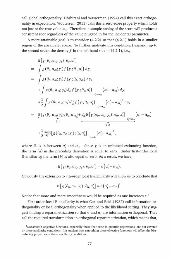
call global orthogonality. Tibshirani and Wasserman (1994) call this exact orthogo-nality in expectation. Woutersen (2011) calls this a zero-score property which holdsnot just at the true value αi0. Therefore, a sample analog of the score will produce aconsistent root regardless of the value plugged in for the incidental parameter.

A more attainable goal is to consider (4.2.2) so that (4.2.1) holds in a smallerregion of the parameter space. To further motivate this condition, I expand, up tothe second order, the density f in the left hand side of (4.2.1), i.e.,

E

g (θ0,αi0; yi) ;θ0,α′i

=ˆ

g (θ0,αi0; yi) f

yi;θ0,α′i

d yi

=ˆ

g (θ0,αi0; yi) f (yi;θ0,αi0) d yi

+ˆ

g (θ0,αi0; yi)∂α′i f

yi;θ0,α′i

α′i=αi0

α′i −αi0

d yi

+12

ˆg (θ0,αi0; yi)∂

2α′i

f

yi;θ0,α′i

α′i=αi0

α′i −αi0

2d yi

= E [g (θ0,αi0; yi) ;θ0,αi0]︸ ︷︷ ︸

(a)

+∂α′iE

g (θ0,αi0; yi) ;θ0,α′i

α′i=αi0︸ ︷︷ ︸

(b)

α′i −αi0

+12∂ 2α′iE

g (θ0,αi0; yi) ;θ0,α′i

α′i= eαi

α′i −αi0

2,

where eαi is in between α′i and αi0. Since g is an unbiased estimating function,the term (a) in the preceding derivation is equal to zero. Under first-order localE-ancillarity, the term (b) is also equal to zero. As a result, we have

E

g (θ0,αi0; yi) ;θ0,α′i

= o

α′i −αi0

.

Obviously, the extension to rth-order local E-ancillarity will allow us to conclude that

E

g (θ0,αi0; yi) ;θ0,α′i

= o

α′i −αi0

r.

Notice that more and more smoothness would be required as one increases r.4

First-order local E-ancillarity is what Cox and Reid (1987) call information or-thogonality or local orthogonality when applied to the likelihood setting. They sug-gest finding a reparametrization so that θ and αi are information orthogonal. Theycall the required transformation an orthogonal reparametrization, which means that,

4Nonsmooth objective functions, especially those that arise in quantile regressions, are not coveredby these ancillarity conditions. It is unclear how smoothing these objective functions will affect the bias-reducing properties of these ancillarity conditions.

77

up to a certain order, estimating αi will have minimal impact on consistently estimat-ing θ . Lancaster (2002) and Woutersen (2011) derive orthogonal reparametriza-tions for common panel data models such as the static single index model withstrictly exogenous regressors and the linear AR(1) dynamic panel data model. Unfor-tunately, finding an orthogonal reparametrization requires finding a solution (whichmay not exist) to a system of partial differential equations.

4.2.2 Implications

Instead of finding solutions to the system of partial differential equations and apply-ing the reparametrization, we can determine how g should be restricted so that gwill satisfy (4.2.2). Notice that rth-order local E-ancillarity is equivalent to searchingfor g such that the following set of moment conditions will hold:

E

g (θ0,αi0; yi)V(k)i (θ0,αi0)

= 0, for k = 1, . . . , r, (4.2.3)

where

V (k)i (θ0,αi0) =∂ kαi

f (yi;θ0,αi0)

f (yi;θ0,αi0)(4.2.4)

is the kth element of the so-called Bhattacharyya basis (see the pioneering works byBhattacharyya (1946; 1947; 1948)).5 To show the equivalence, write the left handside of (4.2.3) as

E

g (θ0,αi0; yi)V(k)i (θ0,αi0)

=ˆ

g (θ0,αi0; yi)∂kα′i

f

yi;θ0,α′i

α′i=αi0

d yi

= ∂ kα′i

ˆg (θ0,αi0; yi) f

yi;θ0,α′i

d yi

α′i=αi0

= ∂ kα′iE

g (θ0,αi0; yi) ;θ0,α′i

α′i=αi0

,

5The Bhattacharyya basis is a natural basis to use when studying the effects of fluctuations of theincidental parameters (around the true value) on the density f (yi ;θ0,αi0). Consider a perturbation inthe incidental parameter from αi0 to α′i . A Taylor series expansion of f about αi0 can be written as thefollowing infinite sum

f

yi ;θ0,α′i

= f (yi ;θ0,αi0) + ∂αif (yi ;θ0,αi0)

α′i −αi0

+ ∂ 2αi

f (yi ;θ0,αi0)

α′i −αi02/2+ · · · .

The likelihood ratio obtained from comparing the perturbed model to the true model can be written as

f

yi ;θ0,α′i

f (yi ;θ0,αi0)= 1+

∂αif (yi ;θ0,αi0)

f (yi ;θ0,αi0)

α′i −αi0

+12

∂ 2αi

f (yi ;θ0,αi0)

f (yi ;θ0,αi0)

α′i −αi02+ · · ·

= 1+ V (1)i (θ0,αi0)

α′i −αi0

+12

V (2)i (θ0,αi0)

α′i −αi02+ · · · .

Relative to the true model, the perturbed model can be “summarized” in terms of an infinite number ofbasis elements of the form V (k)i (θ0,αi0).

78

where the last expression is equal to zero by (4.2.2). Note that whenever an estimat-ing function g satisfies rth-order local E-ancillarity, it also satisfies kth-order localE-ancillarity for all k = 1, . . . , r − 1.

At this point, I will reduce notation by suppressing the arguments (θ0,αi0). I nowshow some of the consequences of (4.2.3) when r = 2. First, note that

E

∂αi0g

= ∂αi0E [g]−E

gV (1)i

= 0, (4.2.5)

which follows from the requirement that g be an unbiased estimating function and(4.2.3) when r = 1. Furthermore, another consequence of (4.2.3) when r = 2 is

Cov

V (1)i ,∂αi0g

= E

V (1)i ∂αi0g

−E

V (1)i

E

∂αi0g

= E

V (1)i ∂αi0g

= 0. (4.2.6)

This zero covariance property follows from calculating the derivative of (4.2.3) withrespect to αi0:

∂αi0E

gV (1)i

= E

gV (2)i

−E

V (1)i ∂αi0g

. (4.2.7)

Since g satisfies first-order local E-ancillarity, the expression E

gV (1)i

on the lefthand side is equal to zero. Since g satisfies second-order local E-ancillarity, the firstterm in the right hand side of (4.2.7) is equal to zero. As a result, the covariancebetween V (1)i and ∂αi0

g is zero whenever g satisfies second-order local E-ancillarity.Finally,

E

∂ 2αi0

g

= ∂αi0E

∂αi0g

−E

V (1)i ∂αi0g

= 0, (4.2.8)

which follows from (4.2.5) and (4.2.6).

It is exactly this zero covariance property (4.2.6), along with the consequences ofsecond-order local E-ancillarity (4.2.5) and (4.2.8), that mimics the bias reductionthat has already been developed in the literature. Estimator-based corrections in thespirit of Hahn and Newey (2004) and Hahn and Kuersteiner (2011) trace the sourceof the bias in the estimator to the O

T−1

bias in the unadjusted score or momentfunction. To illustrate how their work relates to the projected score, I reproduce theircalculation of the bias of some moment function ui t for the common parameter θ .Note that vi t is the moment function for the incidental parameter αi . In the contextof a static panel data model, the bias of ui t is given by

E [ui t (θ ,Òαi)] =1T

§

E

∂αiui t

βi +E

ψi t∂αiui t

+12E

∂ 2αi

ui t

E

ψ2i t

ª

+ o

T−1

,

where ψi t and βi are components of the higher-order asymptotic expansion for Òαi ,i.e.,

ψi t = −E

∂αivi t

−1vi t , βi = −E

∂αivi t

−1§

E

ψi t∂αivi t

+12E

∂ 2αi

vi t

E

ψ2i t

ª

79

Notice that if we chose a moment function ui t such that

E

∂αiui t

= 0, E

ψi t∂αiui t

= 0, E

∂ 2αi

ui t

= 0,

the O

T−1

bias disappears. These three equations are exactly the consequences offirst-order local E-ancillarity, the zero-covariance property in (4.2.6), and second-order local E-ancillarity, respectively. It is in this sense that starting from local E-ancillarity may be more transparent and intuitive when considering bias corrections.

Let us now consider the case of dynamic nonlinear panel data models. In theirmotivation for their bias correction procedure, Hahn and Kuersteiner (2011) showthat the nonzero center of the asymptotic distribution of the uncorrected MLE is

1n

n∑

i=1

1

E

∂αivi t

E

1T

T∑

t=1

vi t

T∑

t=1

∂αiui t

−E

∂ 2αi

ui t

2

E

∂αivi t

2E

1T

T∑

t=1

vi t

2

.

Once again notice that if we choose a moment function for the common parametersui t that satisfies second-order local E-ancillarity, this nonzero center disappears.

In addition to the preceding discussion, the criterion of second-order local E-ancillarity is also constructive because we can interpret (4.2.3) in Hilbert space terms,where the expectation operator is the inner product. We can think of (4.2.3) as find-ing g that is orthogonal to a linear subspace spanned by

V (1)i , . . . , V (r)i

. This linearsubspace represents local effects of incidental parameter fluctuations. An analogousidea appears in linear regression settings so that we can interpret the desired estimat-ing function g as a residual orthogonal to the explanatory variables

V (1)i , . . . , V (r)i

.This residual is called the rth-order projected score. In principle, one can constructthe rth-order projected score but a lot of the benefits in terms of bias correction canalready be reaped at the second order as seen in the preceding discussions.

4.2.3 Computation

Let us consider the situation where one has a complete specification of a likelihoodfor the data. For every i = 1, . . . , n, let zi = (yi0, yi1, . . . , yiT , x i1, . . . , x iT ) be thedata for the ith unit and z = (z1, . . . , zn) be the full data. Let f (zi t ;θ ,αi) be thedensity of the data where θ ∈ Rp and αi ∈ Rq. Assume the cross-sectional units areindependent of each other. The joint density of the observables is given by

f (z;θ ,α) =n∏

i=1

f (zi;θ ,αi) .

Note that the density f (zi;θ ,αi) is specified such that predetermined regressors canbe accommodated. For example, if we let x t

i = (x i1, . . . , x i t) and y ti = (yi0, yi1, . . . , yi t),

80

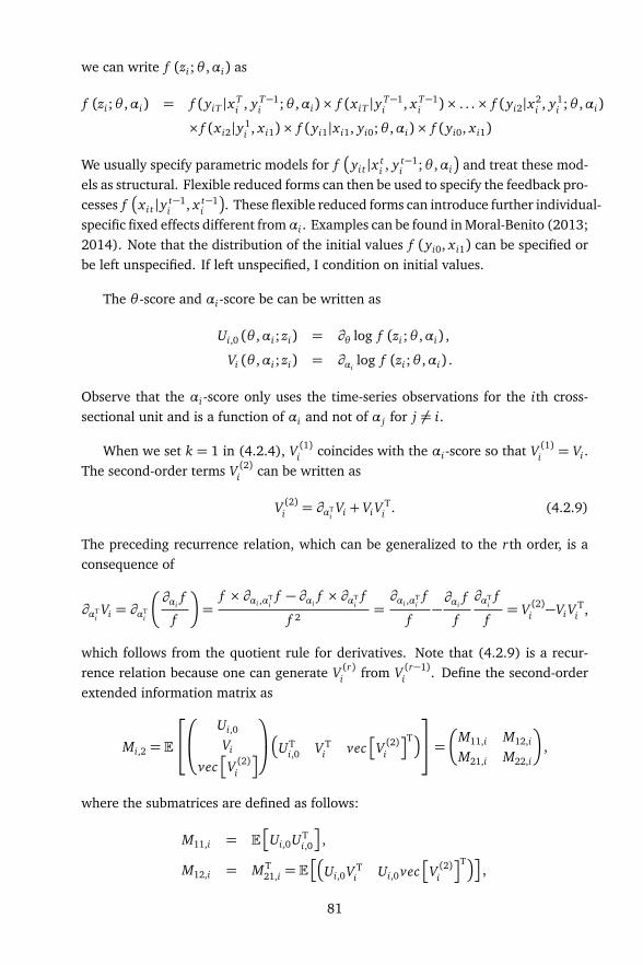
we can write f (zi;θ ,αi) as

f (zi;θ ,αi) = f (yiT |x Ti , y T−1

i ;θ ,αi)× f (x iT |y T−1i , x T−1

i )× . . .× f (yi2|x2i , y1

i ;θ ,αi)

× f (x i2|y1i , x i1)× f (yi1|x i1, yi0;θ ,αi)× f (yi0, x i1)

We usually specify parametric models for f

yi t |x ti , y t−1

i ;θ ,αi

and treat these mod-els as structural. Flexible reduced forms can then be used to specify the feedback pro-cesses f

x i t |y t−1i , x t−1

i

. These flexible reduced forms can introduce further individual-specific fixed effects different fromαi . Examples can be found in Moral-Benito (2013;2014). Note that the distribution of the initial values f (yi0, x i1) can be specified orbe left unspecified. If left unspecified, I condition on initial values.

The θ -score and αi-score be can be written as

Ui,0 (θ ,αi; zi) = ∂θ log f (zi;θ ,αi) ,

Vi (θ ,αi; zi) = ∂αilog f (zi;θ ,αi) .

Observe that the αi-score only uses the time-series observations for the ith cross-sectional unit and is a function of αi and not of α j for j 6= i.

When we set k = 1 in (4.2.4), V (1)i coincides with the αi-score so that V (1)i = Vi .The second-order terms V (2)i can be written as

V (2)i = ∂αTiVi + ViV

Ti . (4.2.9)

The preceding recurrence relation, which can be generalized to the rth order, is aconsequence of

∂αTiVi = ∂αT

i

∂αif

f

=f × ∂αi ,α

Tif − ∂αi

f × ∂αTif

f 2=∂αi ,α

Tif

f−∂αi

f

f

∂αTif

f= V (2)i −ViV

Ti ,

which follows from the quotient rule for derivatives. Note that (4.2.9) is a recur-rence relation because one can generate V (r)i from V (r−1)

i . Define the second-orderextended information matrix as

Mi,2 = E

Ui,0

Vi

vec

V (2)i

UTi,0 V T

i vec

V (2)i

T

=

M11,i M12,i

M21,i M22,i

,

where the submatrices are defined as follows:

M11,i = E

Ui,0UTi,0

,

M12,i = MT21,i = E

Ui,0V Ti Ui,0vec

V (2)i

T

,

81

M22,i = E

Vi

vec

V (2)i

V Ti vec

V (2)i

T

.

The second-order projected score and its information matrix for the ith unit couldbe expressed as

Ui,2 = Ui,0 −M12,i

M22,i

−

Vi

vec

V (2)i

, (4.2.10)

Ii,2 = M11,i −M12,i

M22,i

−M21,i . (4.2.11)

where

M22,i

−is the Moore-Penrose inverse of M22,i . As discussed in the previous

subsection, the second-order projected score is really the residual orthogonal to thelinear subspace spanned by

V (1)i , V (2)i

. Thus, the second-order projected score Ui,2

makes the θ -score Ui,0 less sensitive to the presence of the incidental parameters.The second-order projected score and its associated information matrix for the fulldata can then be computed by summing up n components of the form (4.2.10) and(4.2.11).

As a result of all the preceding discussions, I present the following lemma and amore formal proof in the appendix.

Lemma 4.2.1. The second-order projected score Ui,2 is an unbiased estimating equa-tion that satisfies second-order local E-ancillarity (4.2.2).

In general, the projected score may depend on both θ and αi . Thus, we haveto substitute an estimator for αi to form a plug-in projected score. The first-orderprojected score for the ith unit can be written as

Ui,1 = Ui,0 −E

Ui,0V Ti

E

ViVTi

−Vi .

Solving Vi = 0 gives an estimator for αi given θ , denoted by Òαi (θ ). The plug-infirst-order projected score

∑

idUi,1 coincides with the profile score for θ . Dhaene

and Jochmans (2015b) show that the panel Poisson model and panel exponentialduration model have profile scores that have zero expectation. Therefore, the plug-in first-order projected score mimics the behavior of the profile score when appliedto these models.

On the other hand, the second-order projected score is given by

Ui,2 = Ui,0 −E

Ui,0V Ti

E

ViVTi

−Vi (4.2.12)

−E

Ui,0vec

V (2)i

Th

E

vec

V (2)i

vec

V (2)i

Ti−vec

V (2)i

.

The next two propositions show that the plug-in second-order projected score matchesthe properties of existing bias corrections.

82

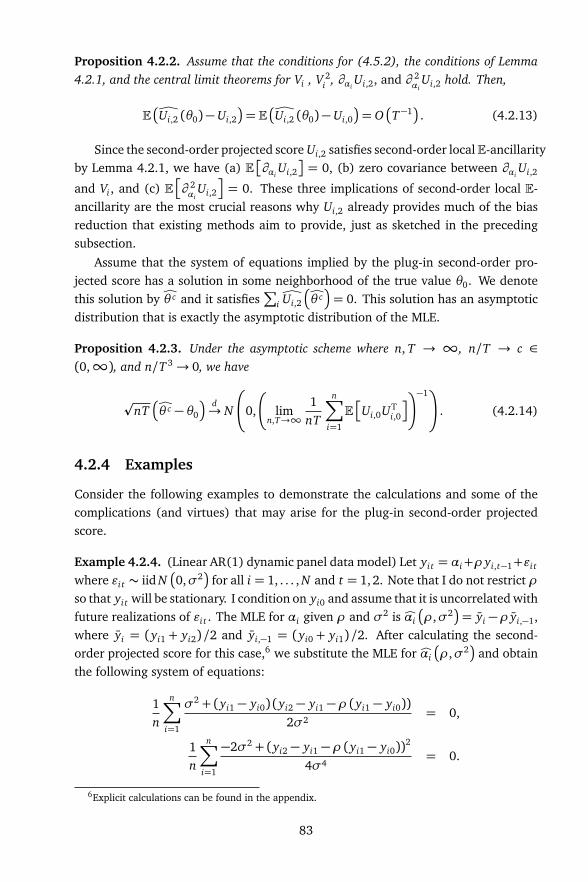
Proposition 4.2.2. Assume that the conditions for (4.5.2), the conditions of Lemma4.2.1, and the central limit theorems for Vi , V 2

i , ∂αiUi,2, and ∂ 2

αiUi,2 hold. Then,

E

dUi,2 (θ0)− Ui,2

= E

dUi,2 (θ0)− Ui,0

= O

T−1

. (4.2.13)

Since the second-order projected score Ui,2 satisfies second-order localE-ancillarityby Lemma 4.2.1, we have (a) E

∂αiUi,2

= 0, (b) zero covariance between ∂αiUi,2

and Vi , and (c) E

∂ 2αi

Ui,2

= 0. These three implications of second-order local E-ancillarity are the most crucial reasons why Ui,2 already provides much of the biasreduction that existing methods aim to provide, just as sketched in the precedingsubsection.

Assume that the system of equations implied by the plug-in second-order pro-jected score has a solution in some neighborhood of the true value θ0. We denotethis solution by cθ c and it satisfies

∑

idUi,2

cθ c

= 0. This solution has an asymptoticdistribution that is exactly the asymptotic distribution of the MLE.

Proposition 4.2.3. Under the asymptotic scheme where n, T → ∞, n/T → c ∈(0,∞), and n/T 3→ 0, we have

pnT

cθ c − θ0

d→ N

0,

limn,T→∞

1nT

n∑

i=1

E

Ui,0UTi,0

−1!

. (4.2.14)

4.2.4 Examples

Consider the following examples to demonstrate the calculations and some of thecomplications (and virtues) that may arise for the plug-in second-order projectedscore.

Example 4.2.4. (Linear AR(1) dynamic panel data model) Let yi t = αi+ρ yi,t−1+εi t

where εi t ∼ iid N

0,σ2

for all i = 1, . . . , N and t = 1, 2. Note that I do not restrict ρso that yi t will be stationary. I condition on yi0 and assume that it is uncorrelated withfuture realizations of εi t . The MLE for αi given ρ and σ2 is Òαi

ρ,σ2

= yi −ρ yi,−1,where yi = (yi1 + yi2)/2 and yi,−1 = (yi0 + yi1)/2. After calculating the second-order projected score for this case,6 we substitute the MLE for Òαi

ρ,σ2

and obtainthe following system of equations:

1n

n∑

i=1

σ2 + (yi1 − yi0) (yi2 − yi1 −ρ (yi1 − yi0))2σ2

= 0,

1n

n∑

i=1

−2σ2 + (yi2 − yi1 −ρ (yi1 − yi0))2

4σ4= 0.

6Explicit calculations can be found in the appendix.

83

Eliminating σ2 from the preceding system gives

2n

n∑

i=1

(yi1 − yi0) (yi2 − yi1 −ρ (yi1 − yi0)) +1n

n∑

i=1

(yi2 − yi1 −ρ((yi1 − yi0)))2 = 0.

Simplifying the equation above gives a quadratic equation in ρ of the form Anρ2 +

Bnρ + Cn = 0 where

An =1n

n∑

i=1

(yi1 − yi0)2,

Bn = −2n

n∑

i=1

(yi2 − yi1) (yi1 − yi0) + (yi1 − yi0)2

,

Cn =1n

n∑

i=1

(yi2 − yi1)2 +

2n

n∑

i=1

(yi1 − yi0) (yi2 − yi1) .

I now show consistency of one of the roots of the quadratic equation. First, assumethat An

p→ A 6= 0. Since Cov (εi2 − εi1, yi1 − yi0) = −σ2, we must have Bn

p→−2ρA+

2σ2−2A and Cnp→ ρ2A−2ρσ2+2ρA. By Slutsky’s lemma, we also have B2

n−4AnCnp→

4

σ2 − A

2. This means that the quadratic equation will always have real roots. Asa result, we have

cρn =−Bn ±

Æ

B2n − 4AnCn

2An

p→ ρ −

σ2

A− 1

±

σ2

A− 1

,

where we either have cρnp→ ρ or cρn

p→ ρ − 2

σ2/A− 1

. The estimator for cσ2n is

given by

cσ2n = −

1n

n∑

i=1

(yi1 − yi0) (yi2 − yi1 −cρn (yi1 − yi0)) ,

and will only be consistent if cρn is consistent. Notice that the roots were obtainedwithout resorting to an iterative procedure unlike the bias correction proposal byBun and Carree (2005).

Which of the two roots should be chosen? To illustrate, consider the case wherewe have stationarity. Assume that yi0 is drawn from its stationary distribution whereE (yi0) = αi/ (1−ρ) and Var (yi0) = σ2/

1−ρ2

, where |ρ| < 1. In this case,

Anp→ 2σ2/ (1+ρ) 6= 0. As a result, σ2/A− 1 < 0. Thus, the consistent root is the

smaller root of the quadratic equation. Now, consider the case where ρ = 1. Notethat the large-n limit of An is such that σ2/A−1< 0 since yi1− yi0 = αi+εi1 impliesthat E (yi1 − yi0)

2 = E (αi + εi1)2 = E

α2i

+σ2 > σ2. As a result, the consistent rootis still the smaller root of the quadratic equation.

84

Dhaene and Jochmans (2015a) extensively document the behavior of the result-ing likelihood obtained after integrating the adjusted profile score. They have shownthat the profile score has a bias that depends only on the common parameters andnot on the incidental parameters. The adjusted profile score is then the difference be-tween the profile score and its bias. They also propose a procedure to choose amongthe multiple critical points of the adjusted likelihood. Extensions of the model thatallow for incidental trends can be found in Moon and Phillips (2004), where theyalso link the second-order projected score to their proposed moment condition.

Allowing for further lags should be straightforward for the projected score be-cause a scalar pth order difference equation can be written as a vector first-orderdifference equation. Therefore, the quadratic equation derived for the AR(1) caseis still going to be a quadratic equation with coefficients that are matrices. Allow-ing for regressors, whether strictly exogenous or predetermined, will not remove themultiple root problem and will have to be examined on a case-by-case basis.

To explore the effect of including a predetermined regressor, consider an exten-sion of the previous example that automatically allows for two individual-specificfixed effects.

Example 4.2.5. (Linear panel VAR(1) model) Consider the following structural modelfor the dynamics of two variables (yi t , x i t):

yi t = φ11 yi,t−1 +φ12 x i,t−1 +ηx i + ε1i t

x i t = φ21 yi,t−1 +φ22 x i,t−1 +ηyi + ε2i t

where the idiosyncratic errors have the following distribution:

ε1i t

ε2i t

∼ N

00

,Σ=

σ11 σ12

σ12 σ22

.

for i = 1, . . . , n and t = 1, 2. Assume that (i) Σ is positive definite, i.e., det (Σ) =σ11σ22 − σ2

12 > 0, (ii) the initial observations (yi0, x i0) are available, and (iii) thedistribution of the fixed effects and initial observations are left unspecified. Thestructural parameters are θ = (φ11,φ12,φ21,φ22,σ11,σ22,σ12). The MLEs for ηx i

and ηyi given the other parameters are

Óηx i =12(yi2 − yi1 (φ11 − 1)−φ11 yi0 −φ12 x i0 −φ12 x i1)

Óηyi =12(x i2 −φ21 yi0 −φ21 yi1 − x i1 (φ22 − 1)−φ22 x i0)

The explicit calculations for the projected score can be carried out in Mathematica.The expectation of the plug-in first-order projected score for the ith cross-sectional

85

unit has nonzero bias, i.e.

E

dUi,1

=

−12

, 0,0,−12

,−σ22

2det (Σ),−

σ11

2 det (Σ),−

σ12

det (Σ)

.

Notice that this nonzero bias does not depend on ηx i and ηyi . As a result, this fits intoCase 2 of Dhaene and Jochmans (2015b), where the profile score has expectationfree of the incidental parameters. Similarly, calculations in Mathematica show thatthe expectation of the plug-in second-order projected score for the ith cross-sectionalunit has zero bias.

Next, I consider a nonlinear model where the score of some conditional likelihoodfor the model is an unbiased estimating equation.

Example 4.2.6. (Static logit model with strictly exogenous regressors) Supposeyi t |xi1,xi2 ∼ Bernoulli (pi t) with probability of success pi t = E (yi t |xi1,xi2) = F(αi +xT

i tβ) for i = 1, . . . , n and t = 1,2. Assume that F is the logistic cdf. For j = 0,1, 2, de-fine N j = i : yi1 + yi2 = j. Following the computations in the appendix, the second-order projected score using all i can be computed as

n∑

i=1

U i2 =

∑

i∈N0

yi2 +∑

i∈N2

(yi2 − 1) +∑

i∈N1

(xi2 − xi1)T

yi2 −1

1+ e(xi2−xi1)Tβ

=∑

i∈N1

(xi2 − xi1)T

yi2 −1

1+ e(xi2−xi1)Tβ

. (4.2.15)

Note that the individuals in N0 and N2 have zero contribution to the plug-in second-order projected score. Although the above expression is monotonically decreasing inβ , there is no closed-form solution to the above estimating equation. Despite this,the plug-in second-order projected score can be shown that this coincides with scoreof the conditional likelihood formed from the units for which yi1 + yi2 = 1. SinceChamberlain (1980) shows that the conditional MLE is

pn-consistent, the same goes

for the root of the plug-in second-order projected score.

Arellano and Bonhomme (2009) derive a bias-reducing prior for this model forgeneral T that removes the O

T−1

bias. Their Monte Carlo simulations includean estimator where the adjustment was iterated. The simulations indicate that theiterated adjustment will mimic the properties of the conditional score when n is fixedand T increased to around 20. In contrast, Dhaene and Jochmans (2015b), who alsoconsider the case of T = 2, show that the conditional score can be obtained eitherby an infinite-order profile score adjustment or by rescaling the profile score by thetotal number of movers. It is unclear whether rescaling will extend to the case whereT > 2.

86

4.3 Simulations

In this section, I show that the finite sample performance of the plug-in second-orderprojected score is as good as or sometimes better than some existing competitors.I focus on panels with a very small value of T for the following reasons. Panelsobtained from developing countries or panels formed from small-scale experimentsusually have single-digit T . In practice, applied researchers will also use a subset ofthe data, especially when there are structural breaks in the time series or when thedata are unbalanced. Therefore, it seems appropriate to choose small values of T togauge finite sample performance.

I implement the projected score method and other alternatives using Mathemat-ica.7 Mathematica allows us to calculate the symbolic representation of the projectedscore and to compute the roots using the FindRoot command. Thus, the user onlyneeds to specify the likelihood function and modify the code for the situation he con-siders without recoding the actual expressions of the corrections.8 Furthermore, thecalculations become much more compact and organized. I use two starting points,namely, the MLEs for the pooled and fixed effects model, for the root-finding algo-rithm. I use the software R to generate the data for the Monte Carlo experimentsand to compute the MLEs (using the routine glm) under the pooled and fixed effectsmodel.9 The draws for the individual-specific fixed effects αi are fixed across 5000replications.

The implementation exploits the comparative advantages of both R and Math-ematica. R can be used to generate samples from a user-specified data generatingprocess and to perform routine estimation procedures, while Mathematica can beused to symbolically calculate the adjusted score and find its roots. The coding stylein the Mathematica notebook allows any end user to do the following:

1. Specify either an objective function or an estimating function based on someparametric model.

2. Use the built-in commands for differentiation and calculation of expectationsto produce symbolic representations of the adjustment found in (4.2.12) .

3. Import data and estimation results. The data and estimation results can comefrom any statistical software capable of exporting its outputs to a text file.

4. Use the programmed functions to generate empirical counterparts of the sym-bolic representations, to calculate roots and produce output for diagnostics,and to generate routine estimation results such as standard errors.

7All Mathematica notebooks and R code are available upon request.8Coding the actual expressions would take an inordinate number of lines of code and would only be

valid for a specific model.9Whenever the MLE does not exist, I take notice of this and I increase the number of replications so

that I could attain the target of 5000 replications.

87

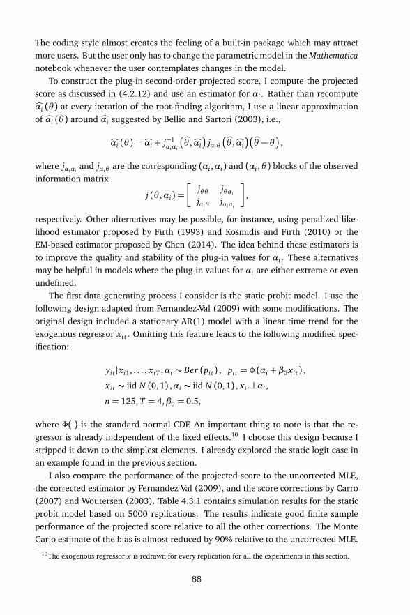
The coding style almost creates the feeling of a built-in package which may attractmore users. But the user only has to change the parametric model in the Mathematicanotebook whenever the user contemplates changes in the model.

To construct the plug-in second-order projected score, I compute the projectedscore as discussed in (4.2.12) and use an estimator for αi . Rather than recomputeÒαi (θ ) at every iteration of the root-finding algorithm, I use a linear approximationof Òαi (θ ) around Òαi suggested by Bellio and Sartori (2003), i.e.,

Òαi (θ ) = Òαi + j−1αiαi

bθ ,Òαi

jαiθ

bθ ,Òαi

bθ − θ

,

where jαiαiand jαiθ

are the corresponding (αi ,αi) and (αi ,θ ) blocks of the observedinformation matrix

j (θ ,αi) =

jθθ jθαi

jαiθjαiαi

,

respectively. Other alternatives may be possible, for instance, using penalized like-lihood estimator proposed by Firth (1993) and Kosmidis and Firth (2010) or theEM-based estimator proposed by Chen (2014). The idea behind these estimators isto improve the quality and stability of the plug-in values for αi . These alternativesmay be helpful in models where the plug-in values for αi are either extreme or evenundefined.

The first data generating process I consider is the static probit model. I use thefollowing design adapted from Fernandez-Val (2009) with some modifications. Theoriginal design included a stationary AR(1) model with a linear time trend for theexogenous regressor x i t . Omitting this feature leads to the following modified spec-ification:

yi t |x i1, . . . , x iT ,αi ∼ Ber (pi t) , pi t = Φ (αi + β0 x i t) ,

x i t ∼ iid N (0,1) ,αi ∼ iid N (0, 1) , x i t⊥αi ,

n= 125, T = 4,β0 = 0.5,

where Φ(·) is the standard normal CDF. An important thing to note is that the re-gressor is already independent of the fixed effects.10 I choose this design because Istripped it down to the simplest elements. I already explored the static logit case inan example found in the previous section.

I also compare the performance of the projected score to the uncorrected MLE,the corrected estimator by Fernandez-Val (2009), and the score corrections by Carro(2007) and Woutersen (2003). Table 4.3.1 contains simulation results for the staticprobit model based on 5000 replications. The results indicate good finite sampleperformance of the projected score relative to all the other corrections. The MonteCarlo estimate of the bias is almost reduced by 90% relative to the uncorrected MLE.

10The exogenous regressor x is redrawn for every replication for all the experiments in this section.

88

As a result, taking higher-order projections may not be needed as the gains will bemarginal relative to computational cost. Furthermore, the standard deviation of theestimator obtained from the projected score is comparable to the standard deviationof the other estimators. The results clearly indicate that score-based corrections maybe preferable in terms of RMSE. Although the number of nonconvergent cases isvery small relative to the number of replications, I recommend obtaining a log of theiterations produced by the root-finding algorithm when implementing score-basedcorrections.

Table 4.3.1: Finite sample performance of estimators of β0Mean Median Standard Median

Estimator bias bias deviation AD RMSEUncorrected MLE 0.210 0.203 0.135 0.089 0.723Fernandez-Val (2009) 0.162 0.156 0.123 0.081 0.674Woutersen (2003) 0.069 0.064 0.099 0.066 0.577(12 cases nonconvergent)Carro (2007) 0.071 0.066 0.100 0.066 0.580(13 cases nonconvergent)Projected score 0.030 0.025 0.095 0.063 0.538Note: True value of β0 is equal to 0.5. Results are based on 5000 replications.

The second data generating process is the first-order dynamic logit model. Oncemore, I adapt the design from Fernandez-Val (2009) with some modifications.

yi t |yi,t−1, . . . , yi0, x i0, x i1, . . . , x iT ,αi ∼ Ber (pi t) , pi t = F

αi +ρ0 yi,t−1 + β0 x i t

,

yi0|x i0, x i1, . . . , x iT ,αi ∼ Ber (pi0) , pi0 = F (αi + β0 x i0) ,

x i t ∼ iid L (0, 1) ,αi ∼ iid L (0, 1) , x i t⊥αi ,

n= 125, T = 3,β0 = 1,ρ0 = 0.5.

In this design, F(·) is the logistic CDF and L(0,1) is the logistic distribution withmean 0 and scale 1. The original design assumes that x i t ∼ N

0,π2/3

and theindividual-specific fixed effects were generated as an average of the four oldest valuesof x i t . I choose to use L (0, 1) because it is quite similar to N

0,π2/3

but withheavier tails. I condition on yi0 instead of using the information from the distributionyi0|x i0, x i1, . . . , x iT in the likelihood function. For this model, the alternatives arethe fixed -T consistent estimator proposed by Honoré and Kyriazidou (2000), thecorrected estimators by Fernandez-Val (2009) and Hahn and Kuersteiner (2011),and the score-based corrections by Carro (2007) and Woutersen (2003).

Recall that Hahn and Kuersteiner (2011) obtain a characterization of the nonzerocenter of the asymptotic distribution of the MLE as discussed in Example 1.2.3.Estimator-based corrections will have to rely on an estimator of this nonzero center.This nonzero center depends on the cross-spectrum of the αi-score and the deriva-

89

tive of the θ -score with respect to αi at the zero frequency and the spectrum of theαi-score at the zero frequency. Since the cross-spectrum and spectrum are infinitesums of cross-covariances and covariances, respectively, a feasible procedure wouldrequire some lag truncation. As a result, we would require an integer bandwidth oflower order than T 1/2 for trimming purposes and for the asymptotic theory to hold.Since T = 3, I set the bandwidth at values 0, 1, and 2.

In contrast, Honoré and Kyriazidou (2000) propose an estimator based on themaximizer of a likelihood conditioned on the subset of observations for which x i2 = x i3.Since this set is a zero probability event given the DGP, a kernel with a correspondingbandwidth is used to give higher weight to observations where x i2 is close to x i3 andgive lower weight to observations otherwise. I use a standard normal kernel for thispurpose. Furthermore, I use the optimal bandwidth derived by Honoré and Kyriazi-dou (2000) which is a constant multiple of T−1/5. I set this constant to values 1, 8,and 64 just as Honoré and Kyriazidou (2000) do so in their own simulations.

The Monte Carlo results in Table 4.3.2 indicate that score-based corrections areperforming quite well relative to estimator-based corrections for the design I con-sider. The bias of the root of the projected score is almost eliminated for both coeffi-cients of the linear predictor. In contrast, the other score-based estimators are havingproblems eliminating the bias in the autoregressive coefficient. There seems to bea point at which a higher bandwidth will not improve finite sample performance ofestimator-based corrections. In fact, the estimator-based correction by Hahn andKuersteiner (2011) almost has the same performance as uncorrected MLE when thebandwidth is equal to 2. Furthermore, the dispersion of the corrected estimators isless than half that of the uncorrected MLE with the exception of the correction byHahn and Kuersteiner (2011). The dispersion of the root of the projected score ismore in line with that of the uncorrected MLE.

I also present two power curves in Table 4.3.1 for the projected score in the dy-namic logit model. I do not present the results for the competing procedures becausethe estimated biases are large relative to the estimated standard deviation. The rejec-tion probability of the test ρ = 0.5 is almost 5% while that of the test β = 1 is about2%. Unfortunately, power is relatively low but this is expected as the asymptoticsrequire a large value for T .

It is clear from the Monte Carlo results that the projected score is a competitivealternative to some of the competing bias-reduction procedures (especially with re-spect to finite sample bias but not in RMSE terms). The biggest downside is thecomputational time. For the designs considered, setting up of the projected score,the calculation of the root, and the standard error calculations took about 2 to 5 min-utes for every replication on a laptop with 8 GB memory and an i7-processor. Evenif we exploit parallel processing, the memory requirement is almost too great for allcores to be used all at once, especially when conducting Monte Carlo simulations.The reason for the high memory requirement is in the nature of the correction – a

90

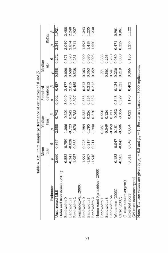
Tabl

e4.

3.2:

Fini

tesa

mpl

epe

rfor

man

ceof

esti

mat

ors

ofβ

andρ

Mea

nM

edia

nSt

anda

rdM

edia

nbi

asbi

asde

viat

ion

AD

RM

SEEs

tim

ator

ρβ

ρβ

ρβ

ρβ

ρβ

Unc

orre

cted

MLE

-2.6

600.

867

-2.5

880.

792

0.90

20.

457

0.55

80.

272

2.34

11.

921

Hah

nan

dKu

erst

eine

r(2

011)

Ban

dwid

th0

-0.5

52-0

.759

-1.0

66-0

.301

3.04

92.

477

0.60

60.

371

3.04

92.

488

Ban

dwid

th1

-0.3

41-0

.028

-0.7

230.

242

2.87

02.

019

0.68

90.

390

2.87

42.

240

Ban

dwid

th2

-1.9

570.

865

-1.8

700.

783

0.89

70.

485

0.53

80.

281

1.71

11.

927

Fern

ande

z-Va

l(20

09)

Ban

dwid

th0

-1.9

940.

225

-1.9

840.

232

0.55

50.

213

0.36

30.

099

1.59

31.

243

Ban

dwid

th1

-1.8

070.

217

-1.7

950.

226

0.55

40.

212

0.36

30.

096

1.41

91.

235

Ban

dwid

th2

-1.9

480.

211

-1.9

400.

220

0.55

20.

212

0.35

90.

095

1.55

01.

230

Hon

oré

and

Kyri

azid

ou(2

000)

Ban

dwid

th1

0.26

80.

550

1.77

10.

885

Ban

dwid

th8

-0.0

490.

126

0.56

10.

265

Ban

dwid

th64

-0.0

590.

131

0.54

10.

250

Wou

ters

en(2

003)

-0.1

83-0

.047

-0.1

81-0

.052

0.34

80.

124

0.23

60.

080

0.47

10.

961

Car

ro(2

007)

-0.5

05-0

.047

-0.5

06-0

.056

0.32

90.

121

0.21

90.

080

0.32

90.

961

(1ca

seno

ncon

verg

ent)

Proj

ecte

dsc

ore

0.01

10.

048

0.00

40.

023

1.17

00.

402

0.36

60.

136

1.27

71.

122

(24

case

sno

ncon

verg

ent)

Not

e:Th

etr

ueva

lues

are

give

nbyρ

0=

0.5

andβ

0=

1.R

esul

tsar

eba

sed

on50

00re

plic

atio

ns.

91

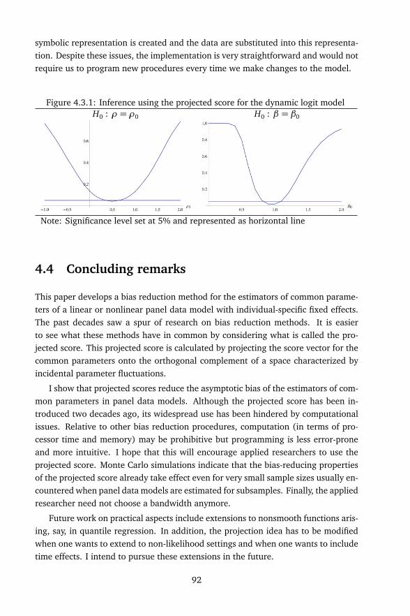
symbolic representation is created and the data are substituted into this representa-tion. Despite these issues, the implementation is very straightforward and would notrequire us to program new procedures every time we make changes to the model.

Figure 4.3.1: Inference using the projected score for the dynamic logit modelH0 : ρ = ρ0 H0 : β = β0

Note: Significance level set at 5% and represented as horizontal line

4.4 Concluding remarks

This paper develops a bias reduction method for the estimators of common parame-ters of a linear or nonlinear panel data model with individual-specific fixed effects.The past decades saw a spur of research on bias reduction methods. It is easierto see what these methods have in common by considering what is called the pro-jected score. This projected score is calculated by projecting the score vector for thecommon parameters onto the orthogonal complement of a space characterized byincidental parameter fluctuations.

I show that projected scores reduce the asymptotic bias of the estimators of com-mon parameters in panel data models. Although the projected score has been in-troduced two decades ago, its widespread use has been hindered by computationalissues. Relative to other bias reduction procedures, computation (in terms of pro-cessor time and memory) may be prohibitive but programming is less error-proneand more intuitive. I hope that this will encourage applied researchers to use theprojected score. Monte Carlo simulations indicate that the bias-reducing propertiesof the projected score already take effect even for very small sample sizes usually en-countered when panel data models are estimated for subsamples. Finally, the appliedresearcher need not choose a bandwidth anymore.

Future work on practical aspects include extensions to nonsmooth functions aris-ing, say, in quantile regression. In addition, the projection idea has to be modifiedwhen one wants to extend to non-likelihood settings and when one wants to includetime effects. I intend to pursue these extensions in the future.

92

4.5 Appendix

Proof of Lemma 4.2.1

To show that Ui,2 is an unbiased estimating equation, we have to show that E

Ui,0

=

0, E [Vi] = 0, and E

vec

V (2)i

= 0. The first two statements follow from the zero-

mean property of the scores. Since E

vec

V (2)i

= vec

E

V (2)i

, we have to show

that E

V (2)i

= 0. Differentiating E [Vi] = 0 with respect to αi gives the desiredresult. Thus, we have shown that Ui,2 is an unbiased estimating equation. To showsecond-orderE-ancillarity, we can show that (4.2.12) satisfies the moment conditionsin (4.2.3) for k = 1,2. This follows by construction.

Proof of Proposition 4.2.2

To simplify the exposition, I return to the case where incidental parameter is scalar.To show (4.2.13), consider a second-order Taylor series expansion of the plug-insecond-order projected score for the ith individual about the true value αi0, i.e.

dUi,2 (θ0) = Ui,2 + ∂αiUi,2 (Òαi (θ0)−αi0) +

12∂ 2αi

Ui,2 (Òαi (θ0)−αi0)2

+Op

T−1/2

. (4.5.1)

Under regularity conditions for maximum likelihood estimation, the three terms in(4.5.1) are Op

T 1/2

, Op

T 1/2

, and Op (1). The final term is a zero mean Op

T−1/2

term. Note that the first-order conditions used to obtain a plug-in estimator for αi

can be expanded in the following way:

ÒVi (θ0) = Vi + ∂αiVi (Òαi (θ0)−αi0) +Op (1) .

Since the right hand size is equal to zero, we can write

Òαi (θ0)−αi0 = −Vi

E

∂αiVi

+Op

T−1

. (4.5.2)

Furthermore, the square of Òαi (θ0)−αi0 can be written as

(Òαi (θ0)−αi0)2

=V 2

i

E

∂αiVi

2 − 2Vi

E

∂αiVi

Op

T−1

+Op

T−2

=V 2

i

E

∂αiVi

2 − 2E (Vi)

E

∂αiVi

Op

T−1

− 2Op

T 1/2

E

∂αiVi

Op

T−1

+Op

T−2

93

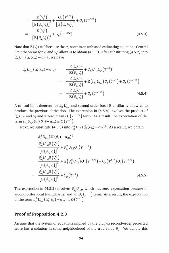
=E

V 2i

E

∂αiVi

2 +Op

T 1/2

E

∂αiVi

2 +Op

T−3/2

=E

V 2i

E

∂αiVi

2 +Op

T−3/2

. (4.5.3)

Note that E (Vi) = 0 because the αi-score is an unbiased estimating equation. Centrallimit theorems for Vi and V 2

i allow us to obtain (4.5.3). After substituting (4.5.2) into∂αi

Ui,2 (Òαi (θ0)−αi0) , we have

∂αiUi,2 (Òαi (θ0)−αi0) = −

Vi∂αiUi,2

E

∂αiVi

+ ∂αiUi,2Op

T−1

= −Vi∂αi

Ui,2

E

∂αiVi

+E

∂αiUi,2

Op

T−1

+Op

T−1/2

= −Vi∂αi

Ui,2

E

∂αiVi

+Op

T−1/2

(4.5.4)

A central limit theorem for ∂αiUi,2 and second-order local E-ancillarity allow us to

produce the previous derivation. The expression in (4.5.4) involves the product of∂αi

Ui,2 and Vi and a zero mean Op

T−1/2

term. As a result, the expectation of theterm ∂αi

Ui,2 (Òαi (θ0)−αi0) is O

T−1

.

Next, we substitute (4.5.3) into ∂ 2αi

Ui,2 (Òαi (θ0)−αi0) 2. As a result, we obtain

∂ 2αi

Ui,2 (Òαi (θ0)−αi0)2

=∂ 2αi

Ui,2E

V 2i

E

∂αiVi

2 + ∂2αi

Ui,2Op

T−3/2

=∂ 2αi

Ui,2E

V 2i

E

∂αiVi

2 +E

∂ 2αi

Ui,2

Op

T−3/2

+Op

T 1/2

Op

T−3/2

=∂ 2αi

Ui,2E

V 2i

E

∂αiVi

2 +Op

T−1

(4.5.5)

The expression in (4.5.5) involves ∂ 2αi

Ui,2, which has zero expectation because of

second-order local E-ancillarity, and an Op

T−1

term. As a result, the expectationof the term ∂ 2

αiUi,2 (Òαi (θ0)−αi0) is O

T−1

.

Proof of Proposition 4.2.3

Assume that the system of equations implied by the plug-in second-order projectedscore has a solution in some neighborhood of the true value θ0. We denote this

94

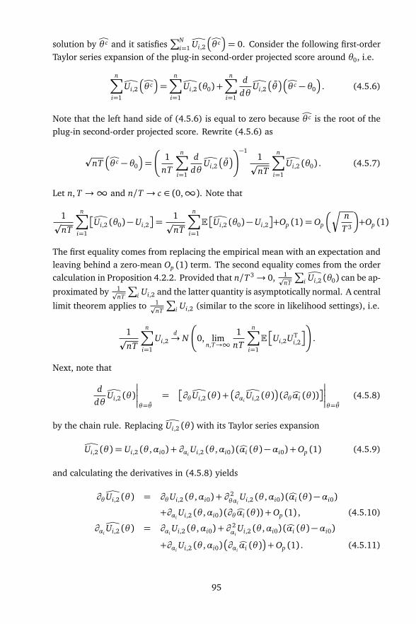
solution by cθ c and it satisfies∑N

i=1dUi,2

cθ c

= 0. Consider the following first-orderTaylor series expansion of the plug-in second-order projected score around θ0, i.e.

n∑

i=1

dUi,2

cθ c

=n∑

i=1

dUi,2 (θ0) +n∑

i=1

ddθ

dUi,2

θ

cθ c − θ0

. (4.5.6)

Note that the left hand side of (4.5.6) is equal to zero because cθ c is the root of theplug-in second-order projected score. Rewrite (4.5.6) as

pnT

cθ c − θ0

=

1nT

n∑

i=1

ddθ

dUi,2

θ

−11p

nT

n∑

i=1

dUi,2 (θ0) . (4.5.7)

Let n, T →∞ and n/T → c ∈ (0,∞). Note that

1p

nT

n∑

i=1

dUi,2 (θ0)− Ui,2

=1p

nT

n∑

i=1

E

dUi,2 (θ0)− Ui,2

+Op (1) = Op

s

nT 3

+Op (1)

The first equality comes from replacing the empirical mean with an expectation andleaving behind a zero-mean Op (1) term. The second equality comes from the ordercalculation in Proposition 4.2.2. Provided that n/T 3→ 0, 1p

nT

∑

idUi,2 (θ0) can be ap-

proximated by 1pnT

∑

i Ui,2 and the latter quantity is asymptotically normal. A central

limit theorem applies to 1pnT

∑

i Ui,2 (similar to the score in likelihood settings), i.e.

1p

nT

n∑

i=1

Ui,2d→ N

0, limn,T→∞

1nT

n∑

i=1

E

Ui,2UTi,2

.

Next, note that

ddθ

dUi,2 (θ )

θ=θ=

∂θdUi,2 (θ ) +

∂αidUi,2 (θ )

(∂θÒαi (θ ))

θ=θ(4.5.8)

by the chain rule. Replacing dUi,2 (θ ) with its Taylor series expansion

dUi,2 (θ ) = Ui,2 (θ ,αi0) + ∂αiUi,2 (θ ,αi0) (Òαi (θ )−αi0) +Op (1) (4.5.9)

and calculating the derivatives in (4.5.8) yields

∂θdUi,2 (θ ) = ∂θUi,2 (θ ,αi0) + ∂2θαi

Ui,2 (θ ,αi0) (Òαi (θ )−αi0)

+∂αiUi,2 (θ ,αi0) (∂θÒαi (θ )) +Op (1) , (4.5.10)

∂αidUi,2 (θ ) = ∂αi

Ui,2 (θ ,αi0) + ∂2αi

Ui,2 (θ ,αi0) (Òαi (θ )−αi0)

+∂αiUi,2 (θ ,αi0)

∂αiÒαi (θ )

+Op (1) . (4.5.11)

95

Taking probability limits, we have the following components:

plimn→∞

1n

n∑

i=1

plimT→∞

1T∂θUi,2 (θ ,αi0)

θ=θ= lim

n,T→∞

1nT

n∑

i=1

E

∂θUi,2

,

plimn→∞

1n

n∑

i=1

plimT→∞

1T∂ 2θαi

Ui,2 (θ ,αi0) (Òαi (θ )−αi0)

θ=θ= 0,

plimn→∞

1n

n∑

i=1

plimT→∞

1T∂αi

Ui,2 (θ ,αi0)

∂αiÒαi (θ )

θ=θ= 0,

plimn→∞

1n

n∑

i=1

plimT→∞

1T∂αi

Ui,2 (θ ,αi0)

θ=θ= 0,

plimn→∞

1n

n∑

i=1

plimT→∞

1T∂ 2αi

Ui,2 (θ ,αi0) (Òαi (θ )−αi0)

θ=θ= 0,

plimn→∞

1n

n∑

i=1

plimT→∞

1T∂αi

Ui,2 (θ ,αi0)

∂αiÒαi (θ )

θ=θ= 0.

Note that as T →∞, we have both θp→ θ0 and Òαi

θ p→ αi0. The second and fifth

equalities follow Òαi

θ p→ αi0 as T → ∞. The third, fourth, and sixth equalities

would follow from the law of large numbers and second-order ancillarity. The Op (1)

terms in (4.5.9), (4.5.10), and (4.5.11) all converge to zero because Òαi

θ p→ αi0 as

T →∞. We can then conclude that

plimn,T→∞

1nT

n∑

i=1

ddθ

dUi,2 (θ )

θ=θ= lim

n,T→∞

1nT

n∑

i=1

E

∂θUi,2

.

Notice that Ui,2 behaves like Ui,0 asymptotically because the correction in (4.2.12)has expectation zero at the true value. As long as the information identity holds,we have E

Ui,2UTi,2

= E

Ui,0UTi,0

= E

∂θUi,0

. Otherwise, we have the usualsandwich-type asymptotic covariance matrix.

Alternative proof of (4.2.14)

In this appendix, we prove the main results in the spirit of the papers by Hahn andNewey (2004) and Hahn and Kuersteiner (2011). We also note some departuresfrom their proof. Let Fi and ÒFi denote the CDF and its empirical counterpart forthe ith individual. Define Fi(ε) = Fi + ε

pT (ÒFi − Fi) and ∆iT =

pT (ÒFi − Fi), where

ε ∈ [0, T−1/2]. We have F(ε) = F+ εp

T (bF− F) in vector form.

Let αi(θ , Fi(ε)) and θ (F(ε)) be the solutions to the estimating equations below:

ˆVi(θ ,αi(θ , Fi(ε));zi) dFi(ε) = 0 (4.5.12)

96

n∑

i=1

ˆUi,2(θ (F(ε)),αi(θ (F(ε)), Fi(ε));z) dFi(ε) = 0 (4.5.13)

The plug-in used for the αi ’s in the second-order projected score can be written asÒαi(θ ) = αi(θ , Fi(T−1/2)). The root for the plug-in version of the second-order pro-jected score can be written as bθ = θ (F(T−1/2)). On the other hand, the true valuescan be written as θ 0 = θ (F(0)) = θ (F) and αi0 = αi(θ , Fi).

Expand the functional θ (bF) about the true value θ (F) up to the third order, i.e.

θ (bF)− θ (F) =1p

Tθ ε(0) +

12

1p

T

2

θ εε(0) +16

1p

T

3

θ εεε(ε) (4.5.14)

where

θ ε(0) = ∂εθ (F(ε))|ε=0, θ εε(0) = ∂ 2ε θ (F(ε))|ε=0, θ εεε(0) = ∂ 3

ε θ (F(ε))|ε=ε∈[0,T−1/2]

(4.5.15)

Define the object

hi(ε) = Ui,2(θ (F(ε)),αi(θ (F(ε)), Fi(ε))) (4.5.16)

where the dependence on the data is suppressed. Hahn and Newey (2004) andHahn and Kuersteiner (2011) use Ui,1 instead of Ui,2. It follows that (4.5.13) can berewritten as

1n

n∑

i=1

ˆhi(ε) dFi(ε) = 0 (4.5.17)

We show that when n, T →∞ such that n/T → c ∈ (0,∞),

pnT (θ (bF)− θ (F))

d→ N

0,

limn,T→∞

1nT

n∑

i=1

Ii

−1!

(4.5.18)

in the following manner:

1. Differentiate (4.5.17) with respect to ε twice. The resulting expressions canbe decomposed into two terms: a term that requires integration with respectto Fi(ε) and a term that characterizes the “tail” or the remainder. We have

1n

n∑

i=1

ˆdhi(ε)

dεdFi(ε) +

1n

n∑

i=1

ˆhi(ε) d∆iT = 0 (4.5.19)

1n

n∑

i=1

ˆd2hi(ε)

dε2dFi(ε) +

2n

n∑

i=1

ˆdhi(ε)

dεd∆iT = 0 (4.5.20)

97

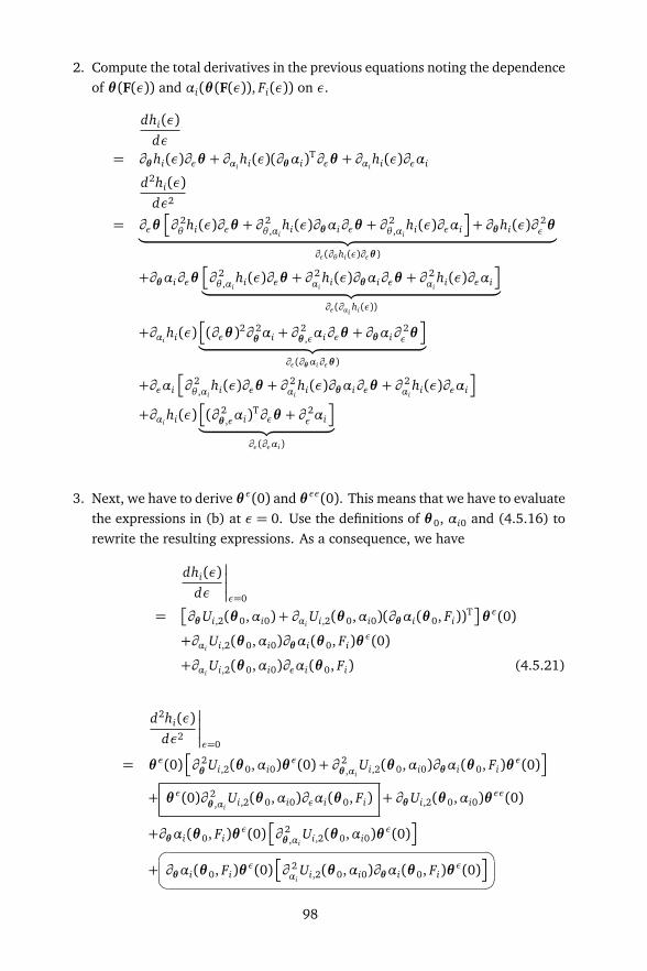
2. Compute the total derivatives in the previous equations noting the dependenceof θ (F(ε)) and αi(θ (F(ε)), Fi(ε)) on ε.

dhi(ε)dε

= ∂θhi(ε)∂εθ + ∂αihi(ε)(∂θαi)

T∂εθ + ∂αihi(ε)∂εαi

d2hi(ε)dε2

= ∂εθ

∂ 2θ hi(ε)∂εθ + ∂

2θ ,αi

hi(ε)∂θαi∂εθ + ∂2θ ,αi

hi(ε)∂εαi

+ ∂θhi(ε)∂2ε θ

︸ ︷︷ ︸

∂ε(∂θhi(ε)∂εθ )

+∂θαi∂εθ

∂ 2θ ,αi

hi(ε)∂εθ + ∂2αi

hi(ε)∂θαi∂εθ + ∂2αi

hi(ε)∂εαi

︸ ︷︷ ︸

∂ε(∂αihi(ε))

+∂αihi(ε)

(∂εθ )2∂ 2θ αi + ∂

2θ ,εαi∂εθ + ∂θαi∂

2ε θ

︸ ︷︷ ︸

∂ε(∂θαi∂εθ )

+∂εαi

∂ 2θ ,αi

hi(ε)∂εθ + ∂2αi

hi(ε)∂θαi∂εθ + ∂2αi

hi(ε)∂εαi

+∂αihi(ε)

(∂ 2θ ,εαi)

T∂εθ + ∂2ε αi

︸ ︷︷ ︸

∂ε(∂εαi)

3. Next, we have to derive θ ε(0) and θ εε(0). This means that we have to evaluatethe expressions in (b) at ε = 0. Use the definitions of θ 0, αi0 and (4.5.16) torewrite the resulting expressions. As a consequence, we have

dhi(ε)dε

ε=0

=

∂θUi,2(θ 0,αi0) + ∂αiUi,2(θ 0,αi0)(∂θαi(θ 0, Fi))

T

θ ε(0)

+∂αiUi,2(θ 0,αi0)∂θαi(θ 0, Fi)θ

ε(0)

+∂αiUi,2(θ 0,αi0)∂εαi(θ 0, Fi) (4.5.21)

d2hi(ε)dε2

ε=0

= θ ε(0)

∂ 2θ Ui,2(θ 0,αi0)θ

ε(0) + ∂ 2θ ,αi

Ui,2(θ 0,αi0)∂θαi(θ 0, Fi)θε(0)

+ θ ε(0)∂ 2θ ,αi

Ui,2(θ 0,αi0)∂εαi(θ 0, Fi) + ∂θUi,2(θ 0,αi0)θεε(0)

+∂θαi(θ 0, Fi)θε(0)

∂ 2θ ,αi

Ui,2(θ 0,αi0)θε(0)

+

∂θαi(θ 0, Fi)θ

ε(0)

∂ 2αi

Ui,2(θ 0,αi0)∂θαi(θ 0, Fi)θε(0)

98

+ ∂θαi(θ 0, Fi)θε(0)

∂ 2αi

Ui,2(θ 0,αi0)∂εαi(θ 0, Fi)

+

∂αi

Ui,2(θ 0,αi0)(θε(0))T∂ 2

θ αi(θ 0, Fi)θε(0)

+ ∂αiUi,2(θ 0,αi0)∂ 2

θ ,εαi(θ 0, Fi)θε(0)

+

∂αi

Ui,2(θ 0,αi0) [∂θαi(θ 0, Fi)θεε(0)]

+ ∂εαi(θ 0, Fi)

∂ 2θ ,αi

Ui,2(θ 0,αi0)θε(0)

+ ∂εαi(θ 0, Fi)

∂ 2αi

Ui,2(θ 0,αi0)∂θαi(θ 0, Fi)θε(0)

+ ∂εαi(θ 0, Fi)

∂ 2αi

Ui,2(θ 0,αi0)∂εαi(θ 0, Fi)

+ ∂αiUi,2(θ 0,αi0)∂ 2

θ ,εαi(θ 0, Fi)θε(0)

+ ∂αiUi,2(θ 0,αi0)∂ 2

ε αi(θ 0, Fi) (4.5.22)

4. Substitute the above expressions into (4.5.19) and (4.5.20). The first sumin (4.5.19) and (4.5.20) when evaluated at ε = 0 becomes the expectationwith respect to the true values while the second sum becomes a “tail” termcharacterizing the difference between the realized distribution ÒFi and the trueone Fi . Since θ ε(0) and θ εε(0) do not depend on the data, they can be treatedas constants with respect to the expectation.

5. We need to derive the expressions for the first and second derivatives ofαi(θ , Fi)with respect to θ and ε. Differentiate (4.5.12) with respect to θ and ε. Solvethe resulting system of two equations in two unknowns for ∂θαi(θ , Fi(ε)) and∂εαi(θ , Fi(ε)). Next, get the second derivatives of (4.5.12) with respect to θand ε. Solve the resulting system of three equations in three unknowns for∂ 2θ αi(θ , Fi(ε)), ∂ 2

θ ,εαi(θ , Fi(ε)), and ∂ 2ε αi(θ , Fi(ε)).11 In effect, we are apply-

ing the Implicit Function Theorem and evaluating at ε = 0 and θ = θ 0. Theresulting first derivatives would be

∂θαi(θ 0, Fi) = −E(∂θV (1)i )

E(∂αiV (1)i )

= Op(1) (4.5.23)

11The systems of equations can be found in the appendix of Hahn and Kuersteiner (2011). Refer topages 1178 and 1181. Solving the system of equations is not as hard as it sounds because the coefficientmatrix is diagonal.

99

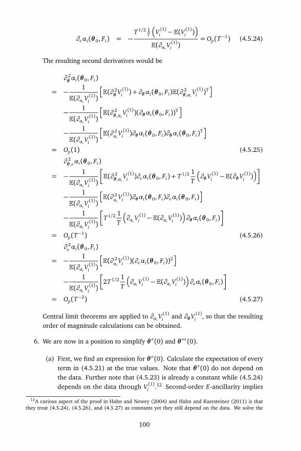
∂εαi(θ 0, Fi) = −T 1/2 1

T

V (1)i −E(V (1)i )

E(∂αiV (1)i )

= Op(T−1) (4.5.24)

The resulting second derivatives would be

∂ 2θ αi(θ 0, Fi)

= −1

E(∂αiV (1)i )

E(∂ 2θ V (1)i ) + ∂θαi(θ 0, Fi)E(∂ 2

θ ,αiV (1)i )

T

−1

E(∂αiV (1)i )

E(∂ 2θ ,αi

V (1)i )(∂θαi(θ 0, Fi))T

−1

E(∂αiV (1)i )

E(∂ 2αi

V (1)i )∂θαi(θ 0, Fi)∂θαi(θ 0, Fi)T

= Op(1) (4.5.25)

∂ 2θ ,εαi(θ 0, Fi)

= −1

E(∂αiV (1)i )

E(∂ 2θ ,αi

V (1)i )∂εαi(θ 0, Fi) + T 1/2 1T

∂θV (1)i −E(∂θV (1)i )

−1

E(∂αiV (1)i )

E(∂ 2αi

V (1)i )∂θαi(θ 0, Fi)∂εαi(θ 0, Fi)

−1

E(∂αiV (1)i )

T 1/2 1T

∂αiV (1)i −E(∂αi

V (1)i )

∂θαi(θ 0, Fi)

= Op(T−1) (4.5.26)

∂ 2ε αi(θ 0, Fi)

= −1

E(∂αiV (1)i )

E(∂ 2αi

V (1)i )(∂εαi(θ 0, Fi))2

−1

E(∂αiV (1)i )

2T 1/2 1T

∂αiV (1)i −E(∂αi

V (1)i )

∂εαi(θ 0, Fi)

= Op(T−2) (4.5.27)

Central limit theorems are applied to ∂αiV (1)i and ∂θV (1)i , so that the resulting

order of magnitude calculations can be obtained.

6. We are now in a position to simplify θ ε(0) and θ εε(0).

(a) First, we find an expression for θ ε(0). Calculate the expectation of everyterm in (4.5.21) at the true values. Note that θ ε(0) do not depend onthe data. Further note that (4.5.23) is already a constant while (4.5.24)depends on the data through V (1)i .12 Second-order E-ancillarity implies

12A curious aspect of the proof in Hahn and Newey (2004) and Hahn and Kuersteiner (2011) is thatthey treat (4.5.24), (4.5.26), and (4.5.27) as constants yet they still depend on the data. We solve the

100

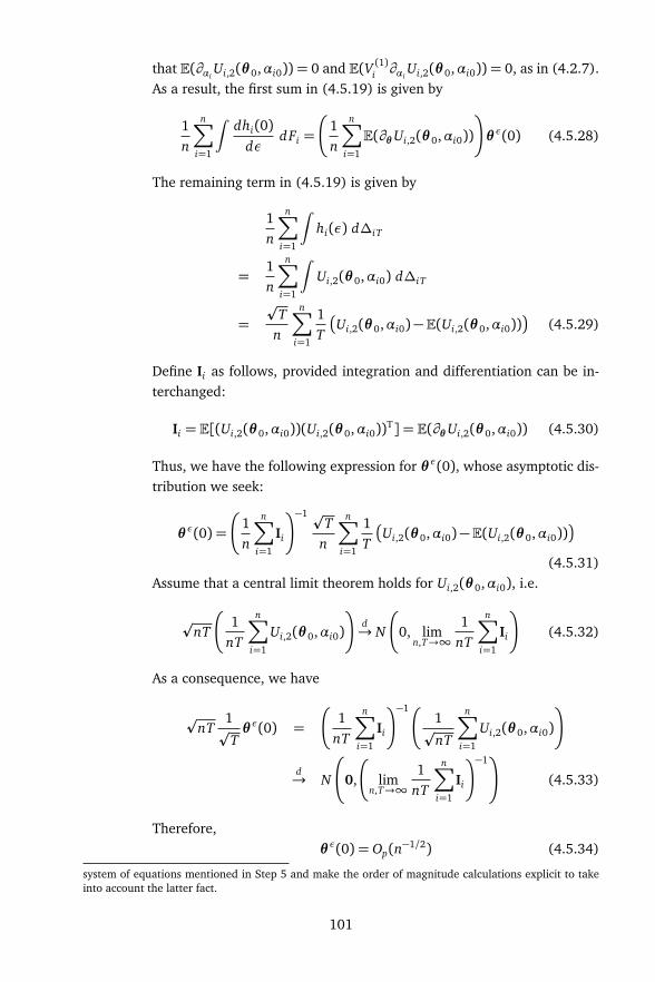
that E(∂αiUi,2(θ 0,αi0)) = 0 and E(V (1)i ∂αi

Ui,2(θ 0,αi0)) = 0, as in (4.2.7).As a result, the first sum in (4.5.19) is given by

1n

n∑

i=1

ˆdhi(0)

dεdFi =

1n

n∑

i=1

E(∂θUi,2(θ 0,αi0))

θ ε(0) (4.5.28)

The remaining term in (4.5.19) is given by

1n

n∑

i=1

ˆhi(ε) d∆iT

=1n

n∑

i=1

ˆUi,2(θ 0,αi0) d∆iT

=p

Tn

n∑

i=1

1T

Ui,2(θ 0,αi0)−E(Ui,2(θ 0,αi0))

(4.5.29)

Define Ii as follows, provided integration and differentiation can be in-terchanged:

Ii = E[(Ui,2(θ 0,αi0))(Ui,2(θ 0,αi0))T] = E(∂θUi,2(θ 0,αi0)) (4.5.30)

Thus, we have the following expression for θ ε(0), whose asymptotic dis-tribution we seek:

θ ε(0) =

1n

n∑

i=1

Ii

−1 pT

n

n∑

i=1

1T

Ui,2(θ 0,αi0)−E(Ui,2(θ 0,αi0))

(4.5.31)Assume that a central limit theorem holds for Ui,2(θ 0,αi0), i.e.

pnT

1nT

n∑

i=1

Ui,2(θ 0,αi0)

d→ N

0, limn,T→∞

1nT

n∑

i=1

Ii

(4.5.32)

As a consequence, we have

pnT

1p

Tθ ε(0) =

1nT

n∑

i=1

Ii

−11p

nT

n∑

i=1

Ui,2(θ 0,αi0)

d→ N

0,

limn,T→∞

1nT

n∑

i=1

Ii

−1!

(4.5.33)

Therefore,θ ε(0) = Op(n

−1/2) (4.5.34)

system of equations mentioned in Step 5 and make the order of magnitude calculations explicit to takeinto account the latter fact.

101

(b) Next we find an expression for θ εε(0). Calculate the expectation of everyterm in (4.5.22) at the true values while noting the orders of magnitude in(4.5.23), (4.5.24), (4.5.25), (4.5.26), (4.5.27), and (4.5.34). The boxed,double-boxed, oval-boxed and unboxed terms in (4.5.22) are Op(n−1/2),Op(T−1), 0, and Op(T n−1) respectively. The first sum in (4.5.20) can nowbe written as

1n

n∑

i=1

ˆd2hi(ε)

dε2dFi(ε) =

1n

n∑

i=1

Ii

θ εε(0)+Op

Tn

+Op

1T

+Op

1p

n

(4.5.35)After applying central limit theorems for ∂θUi,2(θ 0,αi0) and ∂αi

Ui,2(θ 0,αi0)and noting the order of magnitude calculations in (4.5.23), (4.5.24), and(4.5.34), the “tail” term in (4.5.20) can now be written as

2n

n∑

i=1

ˆdhi(ε)

dεd∆iT = Op

1p

n

+Op

1T

(4.5.36)

As a consequence, we have

pnT

1p

T

2

θ εε(0)

=

1nT

n∑

i=1

Ii

−1

Op

1p

nT

+Op

1p

T 3

+Op

s

nT 5

+

1nT

n∑

i=1

Ii

−1

Op

1p

nT 2

+Op

1T 2

Under the conditions that n, T →∞ and n/T → c ∈ (0,∞), the distri-bution of θ εε(0) becomes degenerate at 0.

(c) The last term in the Taylor series expansion (4.5.14) can be shown to beop(1). This step mimics the derivation in Hahn and Kuersteiner (2011).

Projected score for the AR(1) linear dynamic panel data model

The model specification is as follows:

Yi,t−1 = yi0, yi1, . . . , yi,t−1,

yi t |Yi,t−1 ∼ iid N(αi +ρ yi,t−1,σ2), i = 1, . . . , n; t = 1 . . . , T (4.5.37)

Assume yi0 is available and we calculate expectations conditional on yi0 (so that E [·]is the expectation of some expression conditional on yi0). Let ui t = yi t−αi−ρ yi,t−1.The scores for the common parameters ρ and σ2 and the incidental parameter αi

102

are given by:

Uρi,0 =1σ2

T∑

t=1

ui t yi,t−1,

Uσ2

i,0 = −T

2σ2+

12σ4

T∑

t=1

u2i t ,

V (1)i =1σ2

T∑

t=1

ui t .

To calculate the second-order projected score, we need the following elements:

E

(V (1)i )2

=1σ4

E

T∑

t=1

u2i t + 2

∑

t=2

∑

s<t

uisui t

=1σ4

T∑

t=1

σ2 + 2∑

t=2

∑

s<t

E (ui tuis)

=Tσ2

.

Note that only the second moments of (4.5.37) are used for the above calculation

E

V (1)i V (2)i

= −Tσ4

T∑

t=1

E (ui t) +1σ6E

T∑

t=1

ui t

3

=1σ6E

T∑

t=1

ui t

T∑

t=1

u2i t + 2

T∑

t=2

∑

s<t

uisui t

=1σ6

T∑

t=1

E

u3i t

+T∑

t=1

∑

s 6=t

E

u2i tuis

+ 2T∑

r=1

T∑

t=2

∑

s<t

uisui tuir

= 0.

Thus, V (1)i and V (2)i are orthogonal. Note that we used the third moments of (4.5.37)for the preceding calculation

E

(V (2)i )2

=T 2

σ4−

2Tσ6E

T∑

t=1

ui t

2

+1σ8E

T∑

t=1

u2i t + 2

T∑

t=2

∑

s<t

uisui t

2

=T 2

σ4−

2T 2

σ4+

1σ8E

T∑

t=1

u4i t + 2

T∑

t=2

∑

s<t

u2i tu

2is + 4

T∑

t=2

∑

s<t

T∑

r=2

∑

q<r

uiquir

uisui t

= −T 2

σ4+

1σ4[3T + T (T − 1) + 2(T − 1)(T )]

=2T 2

σ4.

103

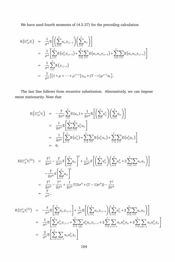
We have used fourth moments of (4.5.37) for the preceding calculation

E

Uρi,0Vi

=1σ4E

T∑

t=1

ui t yi,t−1

T∑

t=1

ui t

=1σ4

T∑

t=1

E

u2i t yi,t−1

+T∑

t=2

∑

s<t

E

ui tuis yi,s−1

+T∑

t=2

∑

s<t

E

ui tuis yi,t−1

=1σ2

T∑

t=1

E

yi,t−1

=1σ2

1+ρ + · · ·+ρT−1

yi0 + (T − t)ρ t−1αi

.

The last line follows from recursive substitution. Alternatively, we can imposemean stationarity. Note that

E

Uσ2

i,0 Vi

= −T

2σ4

T∑

t=1

E (ui t) +1

2σ6E

T∑

t=1

u2i t

T∑

t=1

ui t

=1

2σ6E

T∑

s=1

T∑

t=1

u2i tuis

=1

2σ6

T∑

t=1

E

u3i t

+T∑

t=2

∑

s<t

E

u2i tuis

+T∑

t=2

∑

s<t

E

u2isui t

= 0,

E(Uσ2

i,0 V (2)i ) =T 2

2σ4−

T2σ6

E

T∑

t=1

ui t

2

+1

2σ8E

T∑

t=1

u2i t

T∑

t=1

u2i t + 2

T∑

t=2

∑

s<t

ui tuis

−T

2σ6E

T∑

t=1

ui t

2

=T 2

2σ4−

T 2

2σ4+

12σ8

T (3σ4 + (T − 1)σ4))−T 2

2σ4

=Tσ4

,

E

Uρi,0V (2)i

= −Tσ4E

T∑

t=1

ui t yi,t−1

+1σ6E

T∑

t=1

ui t yi,t−1

T∑

t=1

u2i t + 2

T∑

t=2

∑

s<t

ui tuis

=1σ6E

T∑

t=1

u3i t yi,t−1 +

T∑

t=1

∑

s 6=t

u2isui t yi,t−1 + 2

T∑

t=2

∑

s=t−1

uisu2i t yis + 2

T∑

t=2

∑

s 6=t−1

uisu2i t yis

=2σ6E

T∑

t=2

∑

s=t−1

uisu2i t yis

104

=2σ2(T − t)ρ t−1.

Thus, the second-order projected score for an arbitrary value of T can be com-puted in a straightforward manner using all the components cited above.

Projected score for the static binary choice model with an exoge-nous regressor

Suppose yt |x1, x2 ∼ Ber(pt) with

pt = E(yt |x1, x2) = F(α+ xTt β)≡ Ft

for i = 1, . . . , n and t = 1,2. The uncentered moments of this conditional distributionare all equal to Ft . For this discussion, I suppress the dependence of the expressionon i. Calculations in a separate Mathematica file give the following analytical resultsspecific to the static logit model with one exogenous regressor for T = 2. Let

D1 =

eα+β x1 + 1

eα+β x2 + 1

,

D2 = 4eα+β x1+β x2 + e2α+2β x1+β x2 + e2α+β x1+2β x2 + eβ x1 + eβ x2 .

The scores for β and α are given by

U0 =x1

eα+β x2 + 1

y1

eα+β x1 + 1

− eα+β x1

+ x2

eα+β x1 + 1

y2

eα+β x2 + 1

− eα+β x2

D1

V (1) =−eα

2eα+β x1+β x2 + eβ x1 + eβ x2

+ (y1 + y2)D1

D1

The components of the second-order projected score are calculated below. First,

E

V (1)2=

eαD2

D21

E

V (1)V (2)

=eα

e3α+3β x1+β x2 − e4α+3β x1+2β x2 + e3α+β x1+3β x2 − e4α+2β x1+3β x2

D31

+eα

−eα+2β x1 − eα+2β x2 + eβ x1 + eβ x2

D31

+eα

6eα+β x1+β x2 − 6e3α+2β x1+2β x2

D31

105

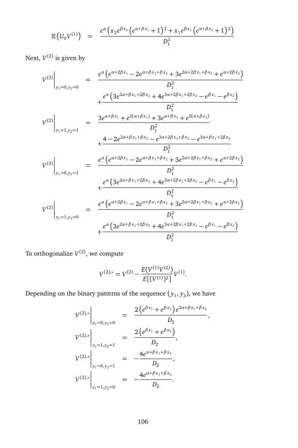
E

U0V (1)

=eα

x2eβ x2

eα+β x1 + 1

2 + x1eβ x1

eα+β x2 + 1

2

D21

Next, V (2) is given by

V (2)

y1=0,y2=0

=eα

eα+2β x1 − 2eα+β x1+β x2 + 3e2α+2β x1+β x2 + eα+2β x2

D21

+eα

3e2α+β x1+2β x2 + 4e3α+2β x1+2β x2 − eβ x1 − eβ x2

D21

V (2)

y1=1,y2=1

=3eα+β x1 + e2(α+β x1) + 3eα+β x2 + e2(α+β x2)

D21

+4− 2e2α+β x1+β x2 − e3α+2β x1+β x2 − e3α+β x1+2β x2

D21

V (2)

y1=0,y2=1

=eα

eα+2β x1 − 2eα+β x1+β x2 + 3e2α+2β x1+β x2 + eα+2β x2

D21

+eα

3e2α+β x1+2β x2 + 4e3α+2β x1+2β x2 − eβ x1 − eβ x2

D21

V (2)

y1=1,y2=0

=eα

eα+2β x1 − 2eα+β x1+β x2 + 3e2α+2β x1+β x2 + eα+2β x2

D21

+eα

3e2α+β x1+2β x2 + 4e3α+2β x1+2β x2 − eβ x1 − eβ x2

D21

To orthogonalize V (2), we compute

V (2),∗ = V (2) −E(V (1)V (2))E[(V (1))2]

V (1).

Depending on the binary patterns of the sequence (y1, y2), we have

V (2),∗

y1=0,y2=0

=2

eβ x1 + eβ x2

e2α+β x1+β x2

D2,

V (2),∗

y1=1,y2=1

=2

eβ x1 + eβ x2

D2,

V (2),∗

y1=0,y2=1

= −4eα+β x1+β x2

D2,

V (2),∗

y1=1,y2=0

= −4eα+β x1+β x2

D2.

106

Hence, we have

E

U0V (2),∗

=2 (x1 − x2)

eβ x2 − eβ x1

e2α+β x1+β x2

D2,

E

V (2),∗2=

4

eβ x1 + eβ x2

e2α+β x1+β x2

D1D2.

The second-order projected score can now be written as

U2 =(x1 − x2)

y21

eβ x1 − eβ x2

+ y1

−eβ x1 + 3eβ x2 + 2y2

eβ x1 − eβ x2

2 (eβ x1 + eβ x2)+(x1 − x2) y2

−3eβ x1 + eβ x2 + y2

eβ x1 − eβ x2

2 (eβ x1 + eβ x2)

Note that we have U2 = 0 over cross-sectional units for which y1+ y2 = 0 or y1+ y2 =2. For cross-sectional units for which y1 + y2 = 1, i.e., substituting in y1 = 1− y2 inthe expression for U2, gives the expression one sees in (4.2.15).

107

108

Chapter 5

The role of sparsity in paneldata models

5.1 Introduction

We have seen increased collection of longitudinal or panel data through active or pas-sive means in recent years. We can study these repeated measurements in three ways– (a) analyze the repeated measurements for each cross-sectional unit separately, (b)analyze the cross-sectional information, and (c) pool the both cross-sectional andtime-series information together.

Methods in time series analysis can be used in situation (a) but will only be feasi-ble when the number of repeated measurements is sufficiently large. The latter caseprecludes studying panels with a short time series dimension, typically collected forpurposes of crafting policy. Methods in cross-sectional analysis can be used in situ-ation (b) but precludes the study of the dynamics of change unless the time seriesdimension is also large. A compromise would then be to use methods that accomplish(c).

Unfortunately, there is much leeway as to how we should pool information avail-able in panel data. Traditionally, econometricians have introduced cross-sectionalheterogeneity in the parameters of a panel data model. Research during the 1960sup to the 1980s, cross-sectional heterogeneity is usually accomplished via the vari-ance components model and the random coefficients model. These models typicallyimpose parametric assumptions on the distribution of heterogeneity so that the di-mension of the parameter space can be reduced substantially. Recent research hasbeen aimed at completely removing these parametric assumptions. Success in thisarea has been mixed but a lot of progress has been made.

109

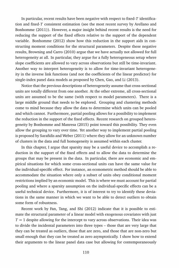
In particular, recent results have been negative with respect to fixed-T identifica-tion and fixed-T consistent estimation (see the most recent survey by Arellano andBonhomme (2011)). However, a major insight behind recent results is the need forreducing the support of the fixed effects relative to the support of the dependentvariable. Bonhomme (2012) show how this reduction in the support aids in con-structing moment conditions for the structural parameters. Despite these negativeresults, Browning and Carro (2010) argue that we have actually not allowed for fullheterogeneity at all. In particular, they argue for a fully heterogeneous setup whereslope coefficients are allowed to vary across observations but still be time-invariant.Another way to interpret heterogeneity is to allow for time-invariant heterogene-ity in the inverse link functions (and not the coefficients of the linear predictor) forsingle-index panel data models as proposed by Chen, Gao, and Li (2013).

Notice that the previous descriptions of heterogeneity assume that cross-sectionalunits are totally different from one another. At the other extreme, all cross-sectionalunits are assumed to be the same (with respect to model parameters). There is alarge middle ground that needs to be explored. Grouping and clustering methodscome to mind because they allow the data to determine which units can be pooledand which cannot. Furthermore, partial pooling allows for a possibility to implementthe reduction in the support of the fixed effects. Recent research on grouped hetero-geneity by Bonhomme and Manresa (2015) point toward this possibility. They evenallow the grouping to vary over time. Yet another way to implement partial poolingis proposed by Sarafidis and Weber (2011) where they allow for an unknown numberof clusters in the data and full homogeneity is assumed within each cluster.

In this chapter, I argue that sparsity may be a useful device to accomplish a re-duction in the support of the fixed effects and to allow the data to determine thegroups that may be present in the data. In particular, there are economic and em-pirical situations for which some cross-sectional units can have the same value forthe individual-specific effect. For instance, an econometric method should be able toaccommodate the situation where only a subset of units obey conditional momentrestrictions implied by an economic model. This is where we must account for partialpooling and where a sparsity assumption on the individual-specific effects can be auseful technical device. Furthermore, it is of interest to try to identify these devia-tions in the same manner in which we want to be able to detect outliers to obtainsome form of robustness.

Recent work by Fan, Tang, and Shi (2012) indicate that it is possible to esti-mate the structural parameter of a linear model with exogenous covariates with justT = 1 despite allowing for the intercept to vary across observations. Their idea wasto divide the incidental parameters into three types – those that are very large thatthey can be treated as outliers, those that are zero, and those that are non-zero butsmall enough that they can be treated as zero asymptotically. I show how to extendtheir arguments to the linear panel data case but allowing for contemporaneously

110

exogenous variables. I also modify their procedure for selecting the data-driven reg-ularization parameter. Unfortunately, not all the results in Fan, Tang, and Shi (2012)survive the extension as we will see in the next section.

Although sparsity has been used in machine learning and big data situations, thefocus has always been settings where the number of covariates is extremely largerelative to the sample size. I restrict myself to the setting where the regressor vec-tor is still finite-dimensional. In contrast, Kock (2013) differences out the incidentalparameters first before proposing a penalty method for the differenced model andallows the regressor vector to be high-dimensional. Kock (2014) extends the previ-ous paper to allow the possibility that the incidental parameters are weakly sparse.In his context, weak sparsity means that the L1 norm of all the incidental parametersis small. As a result, the values of the incidental parameters need not be zero at all.In contrast, I explicitly have zero-valued incidental parameters but allow for some ofthese parameters to be small enough that they can be taken as zero asymptotically.Furthermore, these two papers by Kock are confined to regressors that are strictlyexogenous. Kock and Tang (2014) extends these papers further to dynamic panelsand allow for predetermined regressors. All these developments are under a frame-work where n and T are allowed to vary. Furthermore, their results are in the formof oracle inequalities. These inequalities provide upper bounds for the estimationerror (in some suitable norm) as a function of the design matrix and the dimensionsof the problem.

In contrast, my modifications to Fan, Tang, and Shi (2012) for the panel data caseallow me to consider contemporaneously exogenous regressors and a fixed numberof time periods T . I introduce these modifications and the resulting consequences inSection 5.2. I use Monte Carlo simulations to study the finite sample performance ofthe two-step panel lasso estimator in Section 5.3. I revisit the relationship betweeninequality and growth using the microdata collected by van der Weide and Milanovic(2014). I end with some concluding remarks, suggestions for future research, and atechnical appendix containing some proofs of the main results.

5.2 Panel lasso for the linear model

5.2.1 Setup and notation

Consider the data generating process where

yi t = αi0 + xTi tβ0 + εi t , i = 1, . . . , n; t = 1, . . . , T (5.2.1)

where

α10,α20, . . . ,αN0,β0

are the true values of the parameters and β0 ∈ Rd . Incontrast to the machine learning literature, I assume that d is fixed and does notgrow with sample size. Define the averages xi = T−1

∑Tt=1 xi t and εi = T−1

∑Tt=1 εi t .

111

Let a+ =max a, 0 be the positive part of a, sgn (a) be the sign function, and ‖· ‖2 bethe L2-norm. Let BC

β0

= β ∈ Rd :

β j − β j0

≤ C , 1 ≤ j ≤ d for some constantC > 0. Finally, an bn is shorthand for an is of smaller order than bn and an bn

is shorthand for an is of larger order than bn.

I impose the following assumptions:

A1 (Independence) The errors εi t are independent across i.

A2-1 (Predeterminedness) The errors εi t and the covariates xti = (xi1, . . . ,xi t) satisfy

E(εi t | xti ) = 0 for all i and t.

A2-2 (Contemporaneous exogeneity) The errors εi t and the covariates xi t satisfyE(εi t | xi t) = 0 for all i and t.

A3 (Behavior of averages) Assume that E

‖xi‖2

< ∞ and E (εi) < ∞. Thereexists κn,γn

pn such that, as n→∞, we have

Pr

max1≤i≤n

‖xi‖2 > κn

→ 0, (5.2.2)

Pr

max1≤i≤n

|εi |> γn

→ 0. (5.2.3)

A4 (Sparsity) Each cross-sectional unit i belongs to one and only one of the threepossible index sets 1, . . . , s1, s1 + 1, . . . , s, and s+ 1, . . . , n. If i ∈ 1, . . . , s1,then min1≤i≤s1

|αi0| max κn,γn. If i ∈ s1 + 1, . . . , s, then max1≤i≤n |αi0|<γn. If i ∈ s+ 1, . . . , n, then αi0 = 0.

Assumption A1 is a standard assumption imposed in panel data models without cross-sectional dependence. Assumptions A2-1 or A2-2 allow us to consider dynamics orfeedback effects.1 Implementations of GMM estimators for panel data models usuallymaintain Assumption A2-1 (see Bun and Sarafidis (2015) for a survey). AssumptionA2-2 is usually imposed in pooled OLS (see Wooldridge (2010)). Fan, Tang, andShi (2012) impose assumptions on the behavior of the covariates and the errorssimilar to A3. The difference is that we impose tail behavior assumptions on thetime series averages for every i rather than on the individual values. The existenceof κn,γn

pn is guaranteed by A1 and Markov’s inequality.

Finally, there are three types of incidental parameters by A4 – s1 of them are“large” incidental parameters, s − s1 of them are bounded, and n − s of them arezero. Note that A4 imposes an assumption on the number and the size of the inci-dental parameters. Furthermore, the number of each type of incidental parameter isunknown. With respect to the size of the incidental parameters,

1It is a priori unclear how changing the lasso penalty to other convex or concave penalty functions willaffect the main results.

112

1. Cross-sectional units that belong to the index set 1, . . . , s1 have a “large” valuefor αi0 in the sense that the tail behavior of both the time series averages ofthe regressors and the errors are dominated.

2. Cross-sectional units that belong to the index set i ∈ s1 + 1, . . . , s have a valuefor αi0 that is bounded by the tail behavior of the time series average of theerrors.

3. Cross-sectional units that belong to the index set i ∈ s+ 1, . . . , n have a zerovalue for the incidental parameter.

If we can detect which of the cross-sectional units are zero, then these units can nowbe pooled together to recover a consistent estimator for β0. Unfortunately, the panellasso will have problems distinguishing whether a cross-sectional unit that is not amember of 1, . . . , s1will be classified as bounded or zero. As a result, the panel lassounder the assumptions laid out will not have the oracle property, i.e. the panel lassocannot perform as good as an oracle who knows which of the cross-sectional unitshave αi0 = 0. Nevertheless, the panel lasso produces a fixed-T consistent estimatorbecause it shrinks bounded incidental parameters to zero and this shrinkage has anasymptotically negligible effect.

Note that under large-n asymptotics, the number of each type of incidental pa-rameter may grow with n. We will see later how the growth in the number of eachtype of incidental parameter has to be restricted so that consistency and asymptoticnormality would be obtained. In addition, the size of each type of incidental param-eter may depend on n (at least for the bounded and “large” incidental parameters)as seen in assumption A3 and A4.

Under what circumstances would it be plausible for assumption A4 to hold? Con-sider the following linear model where

yi t = xTi tβ0 +ωi t , i = 1, . . . , n; t = 1, . . . , T. (5.2.4)

Decomposeωi t into E (ωi t |xi t) and its residualωi t−E (ωi t |xi t). Let αi0 = E (ωi t |xi t)be the portion of the errorωi t representing some model deficiency specific to the ithunit that is correlated with the included regressors. Let the residualωi t −E (ωi t |xi t)be equal to εi t . We have now produced (5.2.1) that can potentially satisfy the as-sumptions laid out above from (5.2.4). Therefore, the units for which αi0 = 0 canrepresent the units for which the conditional moment restrictionE (yi t |xi t) = xT

i tβ0 isappropriate. The units for which αi0 are close enough to zero may be treated as zeroasymptotically using the proposed panel lasso estimator. It then becomes importantto detect the units for which there is some serious model deficiency.

The described setting may also apply to situations where we have endogenousregressors but are unable to find valid instruments. Think of αi0 as the unit-specificcorrelation between the errorωi t and xi t . It is possible that only a subset of the units

113

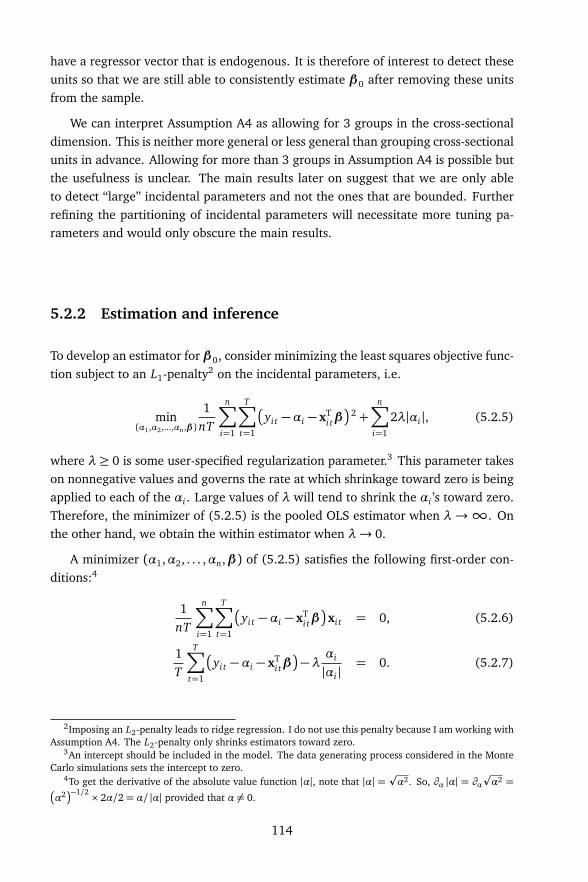
have a regressor vector that is endogenous. It is therefore of interest to detect theseunits so that we are still able to consistently estimate β0 after removing these unitsfrom the sample.

We can interpret Assumption A4 as allowing for 3 groups in the cross-sectionaldimension. This is neither more general or less general than grouping cross-sectionalunits in advance. Allowing for more than 3 groups in Assumption A4 is possible butthe usefulness is unclear. The main results later on suggest that we are only ableto detect “large” incidental parameters and not the ones that are bounded. Furtherrefining the partitioning of incidental parameters will necessitate more tuning pa-rameters and would only obscure the main results.

5.2.2 Estimation and inference

To develop an estimator for β0, consider minimizing the least squares objective func-tion subject to an L1-penalty2 on the incidental parameters, i.e.

min(α1,α2,...,αn,β)

1nT

n∑

i=1

T∑

t=1

yi t −αi − xTi tβ

2 +n∑

i=1

2λ|αi |, (5.2.5)

where λ≥ 0 is some user-specified regularization parameter.3 This parameter takeson nonnegative values and governs the rate at which shrinkage toward zero is beingapplied to each of the αi . Large values of λ will tend to shrink the αi ’s toward zero.Therefore, the minimizer of (5.2.5) is the pooled OLS estimator when λ→∞. Onthe other hand, we obtain the within estimator when λ→ 0.

A minimizer (α1,α2, . . . ,αn,β) of (5.2.5) satisfies the following first-order con-ditions:4

1nT

n∑

i=1

T∑

t=1

yi t −αi − xTi tβ

xi t = 0, (5.2.6)

1T

T∑

t=1

yi t −αi − xTi tβ

−λαi

|αi |= 0. (5.2.7)

2Imposing an L2-penalty leads to ridge regression. I do not use this penalty because I am working withAssumption A4. The L2-penalty only shrinks estimators toward zero.

3An intercept should be included in the model. The data generating process considered in the MonteCarlo simulations sets the intercept to zero.

4To get the derivative of the absolute value function |α|, note that |α| =pα2. So, ∂α |α| = ∂α

pα2 =

α2−1/2 × 2α/2= α/ |α| provided that α 6= 0.

114

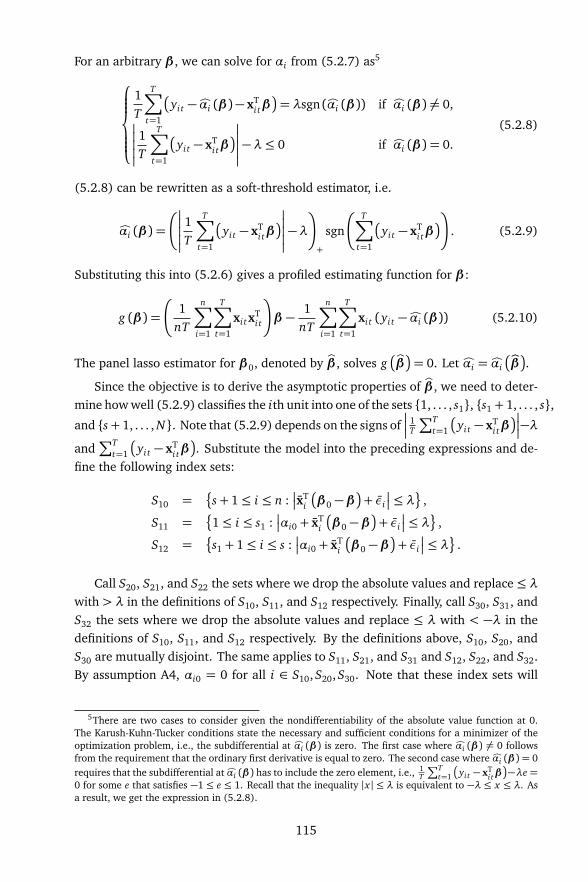
For an arbitrary β , we can solve for αi from (5.2.7) as5

1T

T∑

t=1

yi t − Òαi (β)− xTi tβ

= λsgn (Òαi (β)) if Òαi (β) 6= 0,

1T

T∑

t=1

yi t − xTi tβ

−λ≤ 0 if Òαi (β) = 0.

(5.2.8)

(5.2.8) can be rewritten as a soft-threshold estimator, i.e.

Òαi (β) =

1T

T∑

t=1

yi t − xTi tβ

−λ

+

sgn

T∑

t=1

yi t − xTi tβ

. (5.2.9)

Substituting this into (5.2.6) gives a profiled estimating function for β :

g (β) =

1nT

n∑

i=1

T∑

t=1

xi txTi t

β −1

nT

n∑

i=1

T∑

t=1

xi t (yi t − Òαi (β)) (5.2.10)

The panel lasso estimator for β0, denoted by bβ , solves g

bβ

= 0. Let Òαi = Òαi

bβ

.

Since the objective is to derive the asymptotic properties of bβ , we need to deter-mine how well (5.2.9) classifies the ith unit into one of the sets 1, . . . , s1, s1 + 1, . . . , s,and s+ 1, . . . , N. Note that (5.2.9) depends on the signs of

1T

∑Tt=1

yi t − xTi tβ

−λ

and∑T

t=1

yi t − xTi tβ

. Substitute the model into the preceding expressions and de-fine the following index sets:

S10 =

s+ 1≤ i ≤ n :

xTi

β0 −β

+ εi

≤ λ

,

S11 =

1≤ i ≤ s1 :

αi0 + xTi

β0 −β

+ εi

≤ λ

,

S12 =

s1 + 1≤ i ≤ s :

αi0 + xTi

β0 −β

+ εi

≤ λ

.

Call S20, S21, and S22 the sets where we drop the absolute values and replace ≤ λwith > λ in the definitions of S10, S11, and S12 respectively. Finally, call S30, S31, andS32 the sets where we drop the absolute values and replace ≤ λ with < −λ in thedefinitions of S10, S11, and S12 respectively. By the definitions above, S10, S20, andS30 are mutually disjoint. The same applies to S11, S21, and S31 and S12, S22, and S32.By assumption A4, αi0 = 0 for all i ∈ S10, S20, S30. Note that these index sets will

5There are two cases to consider given the nondifferentiability of the absolute value function at 0.The Karush-Kuhn-Tucker conditions state the necessary and sufficient conditions for a minimizer of theoptimization problem, i.e., the subdifferential at Òαi (β) is zero. The first case where Òαi (β) 6= 0 followsfrom the requirement that the ordinary first derivative is equal to zero. The second case where Òαi (β) = 0requires that the subdifferential at Òαi (β) has to include the zero element, i.e., 1

T

∑Tt=1

yi t − xTi tβ

−λe =0 for some e that satisfies −1 ≤ e ≤ 1. Recall that the inequality |x | ≤ λ is equivalent to −λ ≤ x ≤ λ. Asa result, we get the expression in (5.2.8).

115

depend on β . For an arbitrary index set S, I use bS to denote the result if we plug inthe panel lasso estimator bβ into S.

To analyze whether the panel lasso estimator is consistent, I have to analyzethe components of the estimating equation g

bβ

= 0 after substituting (5.2.1) into(5.2.10):

1nT

n∑

i=1

T∑

t=1

xi txTi t

︸ ︷︷ ︸

Wn

bβ −β0

=1n

n∑

i=1

xiαi0+1

nT

n∑

i=1

T∑

t=1

xi tεi t−1n

n∑

i=1

xiÒαi . (5.2.11)

The last term of (5.2.11) can be rewritten depending on which set i belongs, i.e.

∑

i∈S

xiÒαi =

∑

i∈S

xi xTi

β0 − bβ

+∑

i∈S

xi εi −λ∑

i∈S

xi if S =ÓS20

∑

i∈S

xi xTi

β0 − bβ

+∑

i∈S

xiαi0 +∑

i∈S

xi εi −λ∑

i∈S

xi if S =ÓS21, ÓS22

∑

i∈S

xi xTi

β0 − bβ

+∑

i∈S

xi εi +λ∑

i∈S

xi if S =ÓS30

∑

i∈S

xi xTi

β0 − bβ

+∑

i∈S

xiαi0 +∑

i∈S

xi εi +λ∑

i∈S

xi if S =ÓS31, ÓS32

0 if S =ÓS10, ÓS11, ÓS12

(5.2.12)

To further simplify (5.2.11), we need to say something about the contents of theindex sets defined earlier as n → ∞. But then, we would have to specify how totune the regularization parameter, i.e. I assume that

κn λ, αγn ≤ λ, λp

n, (5.2.13)

where α > 2. This means that λ should be large enough to overrule the tail behaviorof the time series averages of the regressors and the idiosyncratic error but smallenough that it does not overrule the smallest of the “large” incidental parameters.Recall that assumption A4 imposes a particular behavior for the smallest of the “large”incidental parameters. As a result, I am able to extend Lemma 3.1 of Fan, Tang,and Shi (2012) to the panel data case and I present the details of the proof in theappendix.

Lemma 5.2.1 (Contents of index sets). Assume that A1, A2-1 (or A2-2), A3, and A4hold. Let n→∞. For every C > 0 and for every β ∈ BC

β0

, with probability goingto 1,

S10 = S∗10, S11 =∅, S12 = S∗12

S20 =∅, S21 = S∗21, S22 =∅S30 =∅, S31 = S∗31, S32 =∅

where S∗10 = s+ 1, s+ 2, . . . , n, S∗12 = s1 + 1, s1 + 2, . . . , s, S∗21 = 1≤ i ≤ s1 : αi0 > 0and S∗31 = 1≤ i ≤ s1 : αi0 < 0.

116

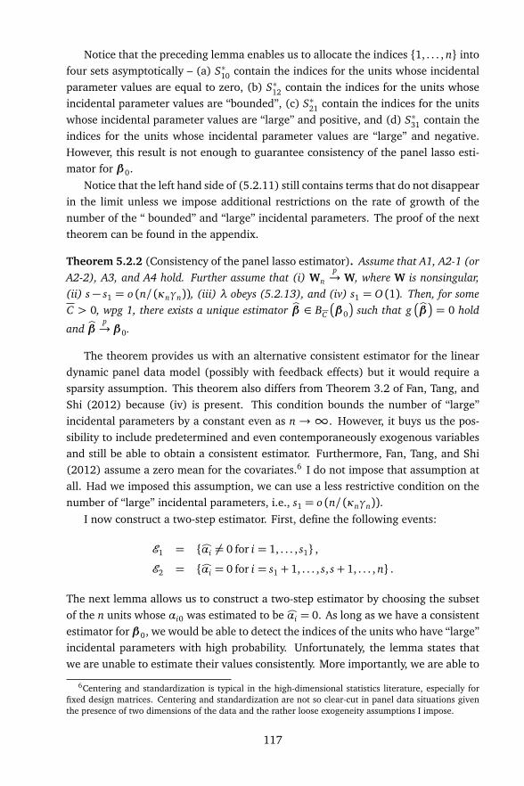
Notice that the preceding lemma enables us to allocate the indices 1, . . . , n intofour sets asymptotically – (a) S∗10 contain the indices for the units whose incidentalparameter values are equal to zero, (b) S∗12 contain the indices for the units whoseincidental parameter values are “bounded”, (c) S∗21 contain the indices for the unitswhose incidental parameter values are “large” and positive, and (d) S∗31 contain theindices for the units whose incidental parameter values are “large” and negative.However, this result is not enough to guarantee consistency of the panel lasso esti-mator for β0.

Notice that the left hand side of (5.2.11) still contains terms that do not disappearin the limit unless we impose additional restrictions on the rate of growth of thenumber of the “ bounded” and “large” incidental parameters. The proof of the nexttheorem can be found in the appendix.

Theorem 5.2.2 (Consistency of the panel lasso estimator). Assume that A1, A2-1 (orA2-2), A3, and A4 hold. Further assume that (i) Wn

p→ W, where W is nonsingular,

(ii) s − s1 = o (n/ (κnγn)), (iii) λ obeys (5.2.13), and (iv) s1 = O (1). Then, for someC > 0, wpg 1, there exists a unique estimator bβ ∈ BC

β0

such that g

bβ

= 0 hold

and bβp→ β0.

The theorem provides us with an alternative consistent estimator for the lineardynamic panel data model (possibly with feedback effects) but it would require asparsity assumption. This theorem also differs from Theorem 3.2 of Fan, Tang, andShi (2012) because (iv) is present. This condition bounds the number of “large”incidental parameters by a constant even as n →∞. However, it buys us the pos-sibility to include predetermined and even contemporaneously exogenous variablesand still be able to obtain a consistent estimator. Furthermore, Fan, Tang, and Shi(2012) assume a zero mean for the covariates.6 I do not impose that assumption atall. Had we imposed this assumption, we can use a less restrictive condition on thenumber of “large” incidental parameters, i.e., s1 = o (n/ (κnγn)).

I now construct a two-step estimator. First, define the following events:

E1 = Òαi 6= 0 for i = 1, . . . , s1 ,

E2 = Òαi = 0 for i = s1 + 1, . . . , s, s+ 1, . . . , n .

The next lemma allows us to construct a two-step estimator by choosing the subsetof the n units whose αi0 was estimated to be Òαi = 0. As long as we have a consistentestimator for β0, we would be able to detect the indices of the units who have “large”incidental parameters with high probability. Unfortunately, the lemma states thatwe are unable to estimate their values consistently. More importantly, we are able to

6Centering and standardization is typical in the high-dimensional statistics literature, especially forfixed design matrices. Centering and standardization are not so clear-cut in panel data situations giventhe presence of two dimensions of the data and the rather loose exogeneity assumptions I impose.

117

detect the zero-valued incidental parameters correctly but we shrink all the boundedincidental parameters to zero. In other words, s1 is identified but not s. The proof isavailable in the appendix.

Lemma 5.2.3 (Partial consistency). Let E = E1 ∩ E2. If bβp→ β0, then Pr (E ) → 1

under A1 to A4.

In principle, the lemma applies to any initial consistent estimator of β0, eventhose that do not explicitly encourage sparsity. An example would be the usual GMMestimator. Unfortunately, the GMM estimator is not available under Assumption A2-2.

We now reestimate (5.2.1) using the data from the subset for which Òαi = 0 usingthis lemma. Define

ÒI0 = 1≤ i ≤ n : Òαi = 0

to be the subset under consideration. Similarly, define the corresponding true indexset, i.e.,

I0 = 1≤ i ≤ n : αi0 = 0 .

The two-step panel lasso estimator eβ can now be defined as the minimizer of

minβ

1nT

∑

i∈ÒI0

T∑

t=1

yi t − xTi tβ

2, (5.2.14)

Notice that (5.2.14) is exactly the least squares objective function restricted to ob-servations belonging to ÒI0. Define the following matrices for i ∈ ÒI0:

Xi =

xTi1

xTi2...

xTiT

, yi =

yi1

yi2...

yiT

, εi =

εi1

εi2...εiT

The solution to (5.2.14) is given by the usual pooled least squares estimator, i.e.,

eβ =

∑

i∈ÒI0

XTi Xi

−1

∑

i∈ÒI0

XTi yi

. (5.2.15)

The next theorem shows that two-step panel lasso estimator eβ is consistent as n→∞. The underlying idea is to use the previous lemma and apply the system OLSconsistency theorem (Theorem 7.1) of Wooldridge (2010), along with an assumptionon the rate of growth of the number of bounded incidental parameters.

118

To be specific, we can rewrite (5.2.15) as

eβ =

∑

i∈ÒI0

XTi Xi

−1

∑

i∈ÒI0

XTi yi

=

∑

i∈ÒI0

XTi Xi

−1

∑

i∈ÒI0

XTi yi

1

ÒI0 6= I0

+ 1

ÒI0 = I0

=

∑

i∈ÒI0

XTi Xi

−1

∑

i∈ÒI0

XTi yi

1

ÒI0 6= I0

︸ ︷︷ ︸

R

+

∑

i∈I0

XTi Xi

!−1 ∑

i∈I0

XTi yi

!

p→ β0 +

plimn→∞

1n

∑

i∈I0

XTi Xi

!−1

plimn→∞

1n

∑

i∈I0

XTi ιTαi0 + plim

n→∞

1n

∑

i∈I0

XTi εi

!

,

where ιT is a T × 1 vector of ones. The term R involve the event

ÒI0 6= I0

, whoseprobability converges to 0 as n →∞ by Lemma 5.2.3. Using assumptions A3 andA4, the term involving the incidental parameters can be evaluated as follows:

1n

∑

i∈I0

XTi ιTαi0

2

=

1n

∑

i∈I0

T xiαi0

2

≤Tn

s∑

i=s1+1

‖xi‖2 |αi0| ≤ T s− s1

n

κnγn.

Here we used assumption A4 to show that αi0 = 0 for i = s + 1, . . . , n. As a result,the term becomes op (1) when s − s1 = o (n/ (κnγn)). Take note that T is taken asfixed here. The term involving the errors has probability limit equal to zero becauseof A2-2. As a result, we have the following theorem:

Theorem 5.2.4 (Consistency of the two-step panel lasso estimator). Suppose that theconditions in Theorem 5.2.2 hold. Further assume that (i) A= E

XTi X i

is nonsingular

and (ii) s− s1 = o (n/ (κnγn)). Then eβp→ β0.

I now show the asymptotic normality of the two-step panel lasso estimator. Notethat the event

pnR= 0

is a subset of the event

ÒI0 6= I0

. As a result, Prp

nR= 0

≤Pr

ÒI0 6= I0

= 0. Consider again the argument earlier for consistency. Recall that

1p

n

∑

i∈I0

XTi ιTαi0

2

≤ T

s− s1pn

κnγn.

The term involving the incidental parameters will only be op (1) when s − s1 =op

n/ (κnγn)

to asymptotically remove the influence of the bounded incidentalparameters. A central limit theorem can then be applied to the term involving the

119

errors. The result then follows from OLS asymptotic normality theorem for systemsof equations (Theorem 7.2) in Wooldridge (2010).

Theorem 5.2.5 (Asymptotic normality of the two-step panel lasso estimator). Sup-pose that the conditions in Theorem 5.2.2 hold. Further assume that (i) A = E

XTi X i

is nonsingular and (ii) s−s1 = op

n/ (κnγn)

. Thenp

n

eβ −β0

d→ N

0,A−1BA−1

,where B= Var

XTi εi

.

Following standard arguments like those in Wooldridge (2010), a consistent es-timator of the asymptotic variance of eβ is given by

bV=

∑

i∈ÒI0

XTi Xi

−1

∑

i∈ÒI0

XTi bεibε

Ti Xi

∑

i∈ÒI0

XTi Xi

−1

,

where bεi = yi −Xieβ = εi −Xi

eβ −β0

is a consistent estimator of εi . Note that thisestimator is a robust variance estimator which allows for arbitrary serial correlationand time-series heteroscedasticity. Finally, note that, in principle, the two-step panellasso reduces to the usual pooled OLS estimator when there is no heterogeneity inαi0.

5.2.3 Choice of regularization parameter

So far we only have a theoretical specification for the regularization parameter λ asseen in (5.2.13). In practice, the choice of λwould have to be data-driven. A feasibleprocedure for the proposed method is as follows:7

1. Apply OLS to the model where yi1 = xTi1β + εi1 for i = 1, . . . , n. Obtain the

residuals from the resulting regression, i.e. cεi1 = yi1 − xTi1ÖβOLS for every i.

2. Select npure observations that correspond to the smallest values of |Óε11| , . . . , |Óεn1|.

3. Apply OLS once again to the model where yi1 = xTi1β + εi1 but only for the

selected npure observations. Obtain the new set of residuals fεi1 = yi1−xTi1àβOLS

for every i = 1, . . . , n.

4. Repeat Step 2 for the new set of residuals |Ýε11| , . . . , |Ýεn1|.

5. Apply the lasso to yi1 = αi0+xTi1β+εi1 but only for the npure observations. The

regularization parameter for this step is the value that minimizes the extendedBIC (EBIC) criterion.

7This feasible procedure has not been studied analytically. Hence, there are no guarantees that theprocedure will mimic the theoretical properties of the panel lasso established earlier.

120

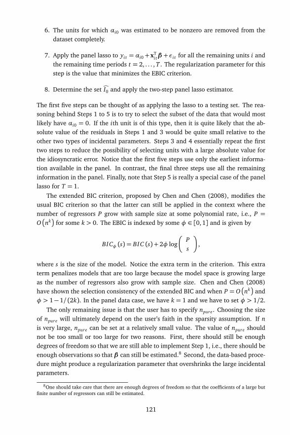
6. The units for which αi0 was estimated to be nonzero are removed from thedataset completely.

7. Apply the panel lasso to yi t = αi0+xTi tβ +εi t for all the remaining units i and

the remaining time periods t = 2, . . . , T . The regularization parameter for thisstep is the value that minimizes the EBIC criterion.

8. Determine the set ÒI0 and apply the two-step panel lasso estimator.

The first five steps can be thought of as applying the lasso to a testing set. The rea-soning behind Steps 1 to 5 is to try to select the subset of the data that would mostlikely have αi0 = 0. If the ith unit is of this type, then it is quite likely that the ab-solute value of the residuals in Steps 1 and 3 would be quite small relative to theother two types of incidental parameters. Steps 3 and 4 essentially repeat the firsttwo steps to reduce the possibility of selecting units with a large absolute value forthe idiosyncratic error. Notice that the first five steps use only the earliest informa-tion available in the panel. In contrast, the final three steps use all the remaininginformation in the panel. Finally, note that Step 5 is really a special case of the panellasso for T = 1.

The extended BIC criterion, proposed by Chen and Chen (2008), modifies theusual BIC criterion so that the latter can still be applied in the context where thenumber of regressors P grow with sample size at some polynomial rate, i.e., P =O

nk

for some k > 0. The EBIC is indexed by some φ ∈ [0,1] and is given by

BICφ (s) = BIC (s) + 2φ log

Ps

,

where s is the size of the model. Notice the extra term in the criterion. This extraterm penalizes models that are too large because the model space is growing largeas the number of regressors also grow with sample size. Chen and Chen (2008)have shown the selection consistency of the extended BIC and when P = O

nk

andφ > 1− 1/ (2k). In the panel data case, we have k = 1 and we have to set φ > 1/2.

The only remaining issue is that the user has to specify npure. Choosing the sizeof npure will ultimately depend on the user’s faith in the sparsity assumption. If nis very large, npure can be set at a relatively small value. The value of npure shouldnot be too small or too large for two reasons. First, there should still be enoughdegrees of freedom so that we are still able to implement Step 1, i.e., there should beenough observations so that β can still be estimated.8 Second, the data-based proce-dure might produce a regularization parameter that overshrinks the large incidentalparameters.

8One should take care that there are enough degrees of freedom so that the coefficients of a large butfinite number of regressors can still be estimated.

121

5.3 Monte Carlo

In this section, I study the finite-sample performance of the two-step panel-lasso esti-mator. I start with the dynamic linear panel data model because this is often used inempirical applications. Furthermore, the empirical application discussed in Section5.4 involves the estimation of a dynamic linear panel data model. The experimentsfollow the Monte Carlo design of Bun and Sarafidis (2015). Their design attempts toencompass existing Monte Carlo designs while ensuring comparability across differ-ent simulations. They consider the following model for i = 1, . . . , n and t = 1, . . . , T :

yi t = 0.8yi,t−1 + 0.2x i t +αi + εi t ,

x i t = 0.95x i,t−1 + 0.25αi +υi t ,

υi t = νi t − 0.1εi t .

I set n to be either 50 or 1000. Assume that εi tiid∼ N (0,1) and νi t

iid∼ N

0,σ2ν

.To better control the experimental conditions, they suggest fixing the values of fourparameters: the signal-to-noise ratio (SNR), the variance ratio (VR) and the correla-tion between the deviation of the initial condition of the x (and y) process(es) fromits long run steady state path and the level of the steady state path itself (rx andry respectively). The signal-to-noise ratio SNR represents the additional varianceprovided by the explained portion of the model conditional on αi0 after netting outthe variance of εi t . The variance ratio VR measures the relative magnitudes of thecumulative impact of the two error components on the average variance of yi t overtime.9

I set SNR = 3, VR = 100, and rx = ry = 0.5. As a consequence, there is alot of noise coming from αi0 relative to other components and the initial conditionsare above the long-run steady state path. I set 40 periods for burn-in.10 The inci-dental parameters αi0 are iid draws from the following mixed discrete-continuousdistribution:

αi0 =

0 with probability p0

W1 (0.5+W2) with probability p1

U [−0.5, 0.5] with probability 1− p0 − p1

,

where W1 = −1 with probability 0.75 and W1 = 1 with probability 0.25 and W2 are iiddraws from the exponential distribution with mean κ. I choose the value of κ so thatI would be able to match the standard deviation of the distribution for the incidental

9For more details on the derivation of these quantities, I refer the reader to Bun and Sarafidis (2015).10Although the number of burn-in periods may be high, mean stationarity is not exactly a requirement

for the panel lasso to work.

122

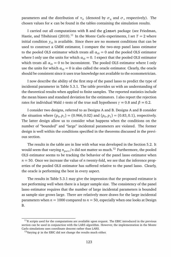
parameters and the distribution of νi t (denoted by ση and σν respectively). Thechosen values for κ can be found in the tables containing the simulation results.

I carried out all computations with R and the glmnet package (see Friedman,Hastie, and Tibshirani (2010).11 In the Monte Carlo experiments, I set T = 2 whereinitial condition yi0 is available. Since there are no moment conditions that can beused to construct a GMM estimator, I compare the two-step panel lasso estimatorto the pooled OLS estimator which treats all αi0 = 0 and the pooled OLS estimatorwhere I only use the units for which αi0 = 0. I expect that the pooled OLS estimatorwhich treats all αi0 = 0 to be inconsistent. The pooled OLS estimator where I onlyuse the units for which αi0 = 0 is also called the oracle estimator. Clearly, the oracleshould be consistent since it uses true knowledge not available to the econometrician.

I now describe the ability of the first step of the panel lasso to predict the type ofincidental parameter in Table 5.3.1. The table provides us with an understanding ofthe theoretical results when applied to finite samples. The reported statistics includethe mean biases and standard deviation for the estimators. I also report the rejectionrates for individual Wald t-tests of the true null hypotheses γ= 0.8 and β = 0.2.

I consider two designs, referred to as Designs A and B. Designs A and B considerthe situation where (p0, p1) = (0.966,0.02) and (p0, p1) = (0.83, 0.1), respectively.The latter design allow us to consider what happens when the conditions on thenumber of “bounded” and “large” incidental parameters are violated. The formerdesign is well within the conditions specified in the theorems discussed in the previ-ous section.

The results in the table are in line with what was developed in the Section 5.2. Itwould seem that varying npure/n did not matter so much.12 Furthermore, the pooledOLS estimator seems to be tracking the behavior of the panel lasso estimator whenn= 50. Once we increase the value of n twenty-fold, we see that the inference prop-erties of the pooled OLS estimator has suffered relative to the panel lasso. Clearly,the oracle is performing the best in every aspect.

The results in Table 5.3.1 may give the impression that the proposed estimator isnot performing well when there is a larger sample size. The consistency of the panellasso estimator requires that the number of large incidental parameters is boundedas sample size grows large. There are relatively more draws for the large incidentalparameters when n= 1000 compared to n= 50, especially when one looks at DesignB.

11R scripts used for the computations are available upon request. The EBIC introduced in the previoussection can be used in conjunction with the LARS algorithm. However, the implementation in the MonteCarlo simulations uses coordinate descent rather than LARS.

12Varying φ in the EBIC did not change the results much either.

123

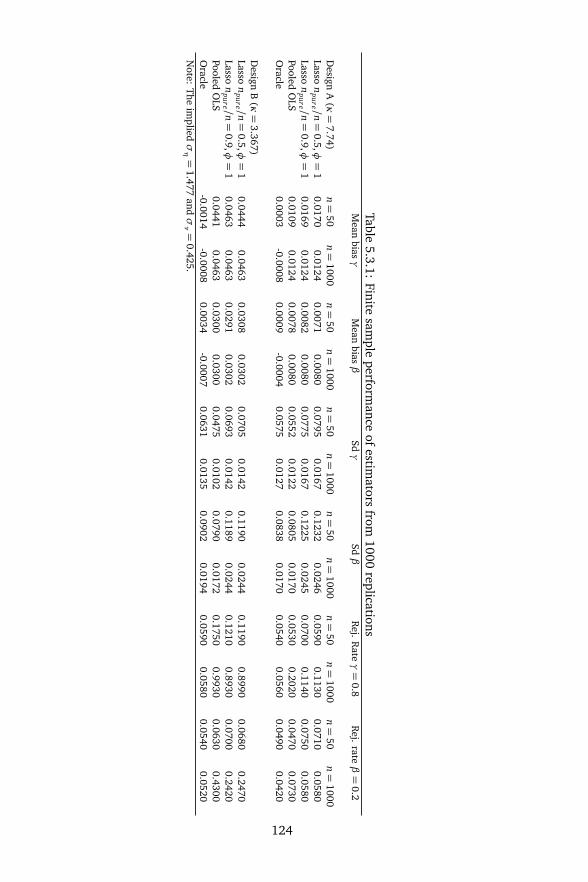
Table5.3.1:

Finitesam

pleperform

anceof

estimators

from1000

replicationsM

eanbias

γM

eanbias

βSdγ

Sdβ

Rej.

Rateγ=

0.8R

ej.rate

β=

0.2

Design

A(κ=

7.74)n=

50n=

1000n=

50n=

1000n=

50n=

1000n=

50n=

1000n=

50n=

1000n=

50n=

1000Lasso

npure /n

=0.5,φ

=1

0.01700.0124

0.00710.0080

0.07950.0167

0.12320.0246

0.05900.1130

0.07100.0580

Lasson

pure /n=

0.9,φ=

10.0169

0.01240.0082

0.00800.0775

0.01670.1225

0.02450.0700

0.11400.0750

0.0580Pooled

OLS

0.01090.0124

0.00780.0080

0.05520.0122

0.08050.0170

0.05300.2020

0.04700.0730

Oracle

0.0003-0.0008

0.0009-0.0004

0.05750.0127

0.08380.0170

0.05400.0560

0.04900.0420

Design

B(κ=

3.367)Lasso

npure /n

=0.5,φ

=1

0.04440.0463

0.03080.0302

0.07050.0142

0.11900.0244

0.11900.8990

0.06800.2470

Lasson

pure /n=

0.9,φ=

10.0463

0.04630.0291

0.03020.0693

0.01420.1189

0.02440.1210

0.89300.0700

0.2420Pooled

OLS

0.04410.0463

0.03000.0300

0.04750.0102

0.07900.0172

0.17500.9930

0.06300.4300

Oracle

-0.0014-0.0008

0.0034-0.0007

0.06310.0135

0.09020.0194

0.05900.0580

0.05400.0520

Note:

Theim

pliedση=

1.477and

σν=

0.425.

124

5.4 Inequality and income growth

The relationship between inequality and income growth has long been a subject ofintense economic debate. Kuznets (1955), one of the top 20 papers chosen to cel-ebrate the centennial of the American Economic Review, precisely deals with thisrelationship. The first page alone already lists down the key issues with studyingthis relationship. I interpret the approach by van der Weide and Milanovic (2014) asone way to address some of the issues with studying this relationship, in particular,the need to start with the family as the unit of analysis. A casual Google search ofthese keywords will already point out the immense number of studies (usually atthe country level) devoted to studying this relationship. As more and more data arecollected and disaggregated, we see more complicated methods being applied likethose that involve dynamic linear panel data methods.

In this section, I revisit the evidence found by van der Weide and Milanovic(2014) where high levels of inequality reduce the income growth of the poorestpercentiles of the distribution. Instead of using readily available aggregate measuresof inequality and income, they construct these aggregate measures using state-leveldata from the United States. Individual-level data from the Integrated Public UseMicrodata Survey for 1960, 1970, 1980, 1990, 2000, and 2010 were used to con-struct state-level measures of income per capita (lnyxx), inequality (gini), educa-tional shortfalls (edushort1518), educational attainment beyond the college level(edu_ms_age2139), share of women outside the labor force (olf_female), shareof household members that are too young (age015) and too old to work (age65).Details regarding the computation and definition of these variables can be found intheir paper.

van der Weide and Milanovic (2014) estimate a Solow-type growth regression atthe state level that includes a measure of inequality as one of the regressors. Theparameter of interest is the effect of income inequality on income growth. Theyestimate (5.2.1) with variables defined as follows:

1. yi t represents income growth at specific percentiles. This is coded as dlnyxxwhere x x ∈ (05,10, 25,50, 75,90, 95,99).13

2. xTi t contain the first-order lags of gini, edu_ms_age2139, edushort1518,age015, age65, olf_female, lnyxx, and time dummies. They also use twoalternative measures of gini, namely, the state-level Gini of the bottom 40%(gini_b40) and top 40% (gini_t40) of the population.14

13It is unclear whether estimating separate regressions for each percentile is preferable over quantileregressions. I leave this to future work.

14They wanted to “unpack” the effect of inequality at the bottom and at the top on income growth atdifferent percentiles.

125

3. They consider data from n = 51 states and T = 5 time periods (representingevery decade since 1960). Alaska and the District of Columbia were consideredoutliers and were excluded from the sample.

I apply the panel lasso estimator to the model just described for T = 2 and for allstates.15 Why would the panel lasso be appropriate in this empirical application?The model chosen in the empirical application can be thought of as a growth re-gression possibly based on an augmented Solow growth model. Just as I discussedin Section 5.2 where I introduced the panel lasso, we can think of the incidentalparameters as representing the suitability or fit of the Solow growth model to thedata. In particular, large non-zero incidental parameters represent states for whichthe growth regression may not be a good approximation. The bounded incidentalparameters represent moderate state-specific deviations from the growth model thatcan be shrunk toward zero (as this would have no effect on the estimator proper-ties, at least asymptotically). An alternative justification is that sparsity can be usefulwhen n and T are both small. The Monte Carlo experiments already provide some ev-idence in this regard. Furthermore, the two-step panel lasso estimator can be appliedeven for T = 2 and even accommodates contemporaneously exogenous regressors.For the moment, there is no estimator that could match these advantages.

The results of the one-step panel lasso estimator indicate that it is possible topool all the states, regardless of whether I use gini as the inequality measure orgini_b40 and gini_t40 as the inequality measures. As a result, the exclusionof Alaska and DC from the sample by van der Weide and Milanovic (2014) may beunwarranted given the results of the one-step panel lasso estimator. The overallconclusion seems to be that heterogeneity across states may not be as large as onemight think.

I then estimate using the proposed two-step panel lasso estimator for T = 2. Ro-bust standard errors are used to construct the confidence intervals. Since the maininterest of van der Weide and Milanovic (2014) is the effect of inequality on incomegrowth, I only present 95% confidence intervals for the slopes of gini, gini_b40,and gini_t40. I set npure/n = 0.8 and φ = 1 for the computation of the regular-ization parameter. I also report results from the pooled OLS estimator where thereis only an overall intercept and no state-specific fixed effects. All other results areavailable upon request.

Figure 5.4.1 already gives an impression that the effect of inequality on incomegrowth for the top 50% of the population has not changed so much over time. Al-though the effect of inequality is mostly positive for the top 50% of the population,the estimated effects are not as large as suggested by the system GMM results ofvan der Weide and Milanovic (2014). In contrast, the effect of inequality on incomegrowth for the bottom 50% of the population has had substantial changes over time.

15Other configurations were implemented but the patterns obtained in Figures 5.4.1 and 5.4.2 remain.

126

If we compare data from 1970-1980 and the decades after, we see that even if theestimated effects are negative (and sometimes close to zero when looking at the me-dian), the absolute values of these estimated effects are getting smaller over time.

Results of pooled OLS estimation can be found in Figure 5.4.2.16 The resultsare substantially different from Figure 5.4.1 in two respects. First, the confidenceintervals obtained by pooled OLS for 1970-1980 are strikingly different from thoseobtained from the two-step panel lasso. Second, the standard errors are much largerfor the panel lasso. I interpret the results of Figure 5.4.2 as evidence that we mayhave to conduct a separate analysis of the 1970-1980 decade. Furthermore, thefigure casts doubt on whether there is parameter constancy over time. The panellasso has somehow stabilized this parameter nonconstancy.

Whichever figure one uses, there seems to be a sharp change in the relationship ofinequality (whether bottom or top or as a whole) and income growth across all per-centiles after 1970-1980. After this sharp change, this relationship has not changedso much after 1990, especially at the top percentiles. Most of the estimated effects ofbottom inequality on income growth are statistically different from zero, especiallyfor the percentiles above the median in recent years. I find that higher bottom in-equality has a positive relationship with income growth at the top percentiles justlike van der Weide and Milanovic (2014) but the magnitudes are slightly smaller.The estimated effects of top inequality on income growth are statistically not differ-ent from zero, especially for the percentiles above the median. If we look at Figures5.4.1 and 5.4.2, there is reason to be optimistic because of the gradual reduction inthe absolute effect of inequality (whether bottom or top or as a whole) on incomegrowth.

To summarize, the results are strikingly different from the reported impression ofmassive inequality during 1990-2010. The absolute effect of bottom or top inequalityon income growth has been getting smaller across time and across percentiles, espe-cially when one looks at the bottom 50% of the population. The sharp change afterthe 1970-1980 decade might be driving the rather negative results (in the sense thatthey find that inequality is good for the rich but not for the poor) of van der Weideand Milanovic (2014). The notion that inequality (whether bottom or top) benefitsonly the rich may be a lot more nuanced than we think.

5.5 Concluding remarks

We show how the penalized least squares approach in the presence of incidental pa-rameters of Fan, Tang, and Shi (2012) can be extended to panel data models. Not

16Pooled OLS is not the same as the panel lasso whenever there are some units for which the incidentalparameter value is not equal to zero. Consider the case where there are cross-sectional units with “large”incidental parameters. The panel lasso removes these units while pooled OLS treats them as if these unitswere no different from units with zero or bounded values for the incidental parameters.

127

all of their results survive the extension. The most serious change in terms of con-sistency and valid inference is the need to bound the number of “large” incidentalparameters by a constant. Despite this, I was able to allow for contemporaneouslyexogenous regressors. The sparsity of incidental parameters has been useful in de-riving consistent estimators for the structural parameters. They come at the cost ofspecifying a particular structure for the asymptotic growth in the different types ofincidental parameters in order to obtain consistency and asymptotic normality. Thelatter has been problematic in the context of estimators that encourage sparsity, asdiscussed extensively by Leeb and Pötscher (2005; 2008).

I also propose a data-based procedure for choosing the regularization parameterwhich uses the extended BIC criterion since the usual BIC criterion is inconsistentwhen the number of parameters grow at a polynomial rate with sample size. Thisdata-based procedure is still at its infancy and would require further study to provideguarantees that coincide with the theory established in the past sections. It is likelythat there would be other algorithms that would perform better than the one I haveproposed.

Results of Monte Carlo experiments indicate good finite sample performance ofthe two-step panel lasso estimator for very small T . Unfortunately, departures fromthe assumed sparsity of the incidental parameters create substantial problems forconsistent estimation and valid inference. As a result, the two-step panel lasso esti-mator is unable to match the performance of the oracle estimator but is preferableto simply using pooled OLS.

I also use the two-step panel lasso estimator to shed light on the relationship be-tween inequality and income growth by revisiting the evidence of van der Weide andMilanovic (2014). The small sample size deters us from making stronger conclusionsabout what makes the excluded states different from the others. Perhaps the mostoptimistic aspect of the results is the gradual move toward the reduced impact ofinequality on income growth across all percentiles.

Although the focus has been on fixed-T consistent estimation, an analysis of theperformance of the penalized least squares estimator under alternative asymptoticembeddings such as letting n, T →∞ jointly or at a particular rate, say n/T → c ∈(0,∞) would be of practical value. The effect of a larger value of T might helpus reduce the restrictions on the growth in the different types of incidental param-eters. This analysis will also give insight as to the statistical benefits of a repeatedobservation and determine whether the cost of collecting panel data is justifiable.Furthermore, the derivation of the asymptotic properties of the two-step panel lassoestimator uses results from seemingly unrelated regressions, as introduced by Zell-ner (1962). Seemingly unrelated regressions give a natural framework for allowingvarying coefficients not just for the intercept term but for the slope coefficients aswell. By allowing for this extension, we may be able to develop alternative estima-tors for the varying coefficients model. Extensions to the case of nonlinear panel data

128

models will also be needed. Finally, linking the properties of the pretest estimatorafter a test of poolability to that of the two-step panel lasso estimator may also be ofpractical value. I leave all these to future research.

5.6 Appendix

Proof of Lemma 5.2.1

The argument follows Fan, Tang, and Shi (2012) but with some modifications andcorrections. Let C be an arbitrary (small) positive number and β ∈ BC

β0

.

We first prove that S10 = S∗10, S20 = ∅, S30 = ∅ wpg 1. It is always true thatS10 ⊆ S∗10. Thus we have to show that Pr

S10 ⊇ S∗10

→ 1. Define the events B =

max1≤i≤n ‖xi‖2 ≤ κn

andD = s+ 1≤ i ≤ n : |εi |< γn. Note that Pr

S10 ⊇ S∗10

≥Pr

S10 ⊇ S∗10 | B

Pr (B). Since Pr (B) → 1 by assumption A3, it suffices to showthat Pr

S10 ⊇ S∗10 | B

→ 1. For large n, Pr

S∗10 ⊆ D

→ 1. Conditional on B ,|εi | ≤ γn implies that

xTi

β0 −β

+ εi

≤

xTi

β0 −β

+ |εi | ≤

xTi

2

β0 −β

2 + |εi | ≤ κn

p

dC + γn,

and we have κn

pdC + γn ≤ λ for large n by (5.2.13). As a result, D ⊆ S10. Thus,

Pr

S∗10 ⊆ D ⊆ S10 | B

→ 1. Since S10 ∪S20 ∪S30 = S∗10 is always true, we must haveS20 =∅ and S30 =∅ wpg 1.

Next we prove that S11 = ∅, S21 = S∗21, S31 = S∗31 wpg 1. We show that S21 = S∗21

wpg 1 as the case for S31 = S∗31 wpg 1 is analogous. . Let S211 = S21 ∩ S∗21 andS212 = S21 ∩

S∗21

c. It suffices to show that Pr

S211 = S∗21

→ 1 and Pr (S212 =∅)→1. It is always true that S21 ⊆ S∗21. Thus we have to show that Pr

S21 ⊇ S∗21

→ 1.Define the eventsB =

max1≤i≤n ‖xi‖2 ≤ κn

andD = 1≤ i ≤ s1 : εi ≥ −γn. Notethat Pr

S21 ⊇ S∗21

≥ Pr

S21 ⊇ S∗21 | B

Pr (B). Since Pr (B) → 1 by assumptionA3, it suffices to show that Pr

S211 ⊇ S∗21 | B

→ 1. For large n, Pr

S∗21 ⊆ D

→ 1.Conditional onB and noting that αi0 > 0, εi > −γn implies that

αi0 + xTi

β0 −β

+ εi > α∗ − κn

p

dC − γn,

and we have α∗ − κn

pdC − γn ≥ λ for large n by (5.2.13). As a result, D ⊆ S211.

Thus, Pr

S∗21 ⊆ D ⊆ S211 | B

→ 1.

Now, we show that Pr (S212 =∅)→ 1. It is always true that ∅ ⊆ S212. Thus wehave to show that Pr (S212 ⊆∅)→ 1. Define the eventsB =

max1≤i≤n ‖xi‖2 ≤ κn

and D = 1≤ i ≤ s1 : εi > γn. Note that Pr (S212 ⊆∅) ≥ Pr (S212 ⊆∅ | B)Pr (B).Since Pr (B)→ 1 by assumption A3, it suffices to show that Pr (S212 ⊆∅ | B)→ 1.For large n, Pr (D ⊆∅)→ 1. Conditional on B , noting that αi0 < 0 and γn − α∗ +

129

κn

pdC < λ for large n by (5.2.13), αi0 + xT

i (β∗ −β) + εi > λ implies that

εi > λ−αi0 − xTi

β0 −β

> λ+α∗ −κn

p

dC > γn.

As a result, S212 ⊆ D. Thus, Pr (S212 ⊆ D ⊆∅ | B)→ 1. Along with Pr

S∗21 ⊆ S211 | B

→1, we have S21 = S∗21 wpg 1.

Finally, we prove that S12 = S∗12, S22 = ∅, S32 = ∅ wpg 1. It is always true thatS12 ⊆ S∗12. Thus we have to show that Pr

S12 ⊇ S∗12

→ 1. Define the events B =

max1≤i≤n ‖xi‖2 ≤ κn

andD = s1 + 1≤ i ≤ s : |εi |< γn. Note that Pr

S12 ⊇ S∗12

≥Pr

S12 ⊇ S∗12 | B

Pr (B). Since Pr (B) → 1 by assumption A3, it suffices to showthat Pr

S12 ⊇ S∗12 | B

→ 1. For large n, Pr

S∗12 ⊆ D

→ 1. Conditional on B ,|εi | ≤ γn implies that

αi0 − κn

p

dC − γn ≤ αi0 + xTi

β0 −β

+ εi ≤ αi0 +κn

p

dC + γn,

and we have −λ − αi0 + κn

pdC < −γn and λ − αi0 − κn

pdC > γn for large n by

(5.2.13). As a result, D ⊆ S12. Thus, Pr

S∗12 ⊆ D ⊆ S12 | B

→ 1. Since S12 ∪ S22 ∪S32 = S∗12 is always true, we must have S22 =∅ and S32 =∅ wpg 1.

Proof of Theorem 5.2.2

We now analyze every term in (5.2.11) after substituting in (5.2.12) and applyingLemma 5.2.1:

1. Collect all the terms that involve αi0. Under A3 and A4, we have

1n

∑

i∈S∗12

xiαi0

2

≤1n

∑

i∈S∗12

‖xi‖2 |αi0| ≤s− s1

nκnγn.

Provided that s− s1 = o (n/ (κnγn)), we have1n

n∑

i=1

xiαi0 = op (1).

2. By the law of large numbers along with A1,

1nT

n∑

i=1

T∑

t=1

xi tεi tp→ lim

n→∞

1nT

n∑

i=1

T∑

t=1

E(xi tεi t) = 0.

The latter equality follows from A2-1 or A2-2 or even strict exogeneity.

3. Strict exogeneity of xi t allows us to conclude that1n

n∑

i=1

xi εip→ 0. If any of the

variables in xi t is predetermined or weakly exogenous, the argument has to

130

change slightly, i.e.

1n

∑

i∈S∗21∪S∗31

xi εi

2

≤1n

∑

i∈S∗21∪S∗31

‖xi εi‖2 ≤s1

nκnγn.

The latter is o (1) when s1 = o (n/ (κnγn)).

4. Let S = S∗21, S∗31. Note that

λ

n

∑

i∈S

xi

2

≤λ

n

∑

i∈S

‖xi‖2 ≤λ

ns1κn =

λp

ns1κnp

n.

The latter will only be op (1) when A3 holds, λ obeys (5.2.13), and s1 = O (1).

Proof of Lemma 5.2.3

Let E = E1 ∩E2. Assume that bβp→ β0. Define the following probabilities:

T0 = Pr

n⋂

i=s+1

xTi

β0 − bβ

+ εi

≤ λ

T1 = Pr

s1⋂

i=1

αi0 + xTi

β0 − bβ

+ εi > λ

T2 = Pr

s⋂

i=s1+1

αi0 + xTi

β0 − bβ

+ εi

≤ λ

Notice that Pr (E ) = T0T1T2. Therefore, to show that Pr (E )→ 1 , it suffices to showthat T0→ 1, T1→ 1, and T2→ 1. Note that

1− T1 = Pr

s1⋃

i=1

αi0 + xTi

β0 − bβ

+ εi ≤ λ

≤ Pr

⋃

i∈S∗21

αi0 + xTi

β0 − bβ

+ εi ≤ λ

!

︸ ︷︷ ︸

T11

+Pr

⋃

i∈S∗31

αi0 + xTi

β0 − bβ

+ εi ≤ λ

!

︸ ︷︷ ︸

T12

.

131

We just have to show that T11 → 0 and T12 → 0. Define C =n

β0 − bβ

2< C

o

where C = (α− 1)/

Mαp

d

> 0, for some choice of M . Note that

T11 ≤ Pr

⋃

i∈S∗21

αi0 + xTi

β0 − bβ

+ εi ≤ λ

∩C

!

+ Pr (C c)

≤ Pr

⋃

i∈S∗21

¦

εi ≤ λ−α∗ + κnCp

d©

!

+ Pr (C c)

≤ Pr

⋃

i∈S∗21

[εi ≤ −γn]

!

+ Pr (C c)

≤ s1 Pr (εi ≤ −γn) + Pr (C c)→ 0.

The first inequality follows from the law of total and probability and the monotonic-ity of the probability function. The second inequality follows from the definition ofC and the characteristics of the incidental parameters belong to the set S∗21. Thethird and fourth inequalities follows from the specification of the regularization pa-rameter found in (5.2.13) and subadditivity. The convergence to zero follows fromassumption A3 and the consistency of the panel lasso. An analogous derivation willshow that T12→ 0.

To show that T0→ 1, note that

T0 ≥ Pr

n⋂

i=s+1

−λ− xTi

β0 − bβ

≤ εi ≤ λ− xTi

β0 − bβ

∩C

≥ Pr

n⋂

i=s+1

−γn ≤ εi ≤ γn

→ 1.

The first inequality follows from the monotonicity of the probability function andsome algebra. The second inequality arises because λ obeys (5.2.13) and

−λ− xTi

β0 − bβ

≤ −λ+

xTi

2

β0 − bβ

2≤ −λ+κnC

p

d

≤ −λ+λMCp

d = λ

MCp

d − 1

< λ

−1α

≤ −γn

for the choice of C indicated earlier.

132

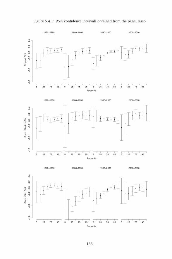
Figure 5.4.1: 95% confidence intervals obtained from the panel lasso

Percentile

Slo

pe o

f G

ini

1970−1980 1980−1990 1990−2000 2000−2010

−1.0

−0.6

−0.2

0.0

0.2

0.4

5 25 75 955 25 75 955 25 75 955 25 75 95

Percentile

Slo

pe o

f bottom

Gin

i

1970−1980 1980−1990 1990−2000 2000−2010

−1.0

−0.6

−0.2

0.0

0.2

0.4

5 25 75 955 25 75 955 25 75 955 25 75 95

Percentile

Slo

pe o

f to

p G

ini

1970−1980 1980−1990 1990−2000 2000−2010

−1.0

−0.6

−0.2

0.0

0.2

0.4

5 25 75 955 25 75 955 25 75 955 25 75 95

133

Figure 5.4.2: 95% confidence intervals obtained from pooled OLS

Percentile

Slo

pe o

f G

ini

1970−1980 1980−1990 1990−2000 2000−2010

−1.0

−0.6

−0.2

0.0

0.2

0.4

5 25 75 955 25 75 955 25 75 955 25 75 95

Percentile

Slo

pe o

f bottom

Gin

i

1970−1980 1980−1990 1990−2000 2000−2010

−1.0

−0.6

−0.2

0.0

0.2

0.4

5 25 75 955 25 75 955 25 75 955 25 75 95

Percentile

Slo

pe o

f to

p G

ini

1970−1980 1980−1990 1990−2000 2000−2010

−1.0

−0.6

−0.2

0.0

0.2

0.4

5 25 75 955 25 75 955 25 75 955 25 75 95

134

Chapter 6

Summary

My thesis is a collection of essays with a common theme: what practices and meth-ods can be considered appropriate responses to the incidental parameter problemin panel data models. In recent years, we have seen an explosion of data collectedfrom individuals, firms, or countries across short or long periods of time. This typeof data gives us an opportunity to study the dynamics of change while controlling fortime-invariant unobserved heterogeneity. Unfortunately, time-invariant unobservedheterogeneity, which is usually in the form of individual-specific fixed effects, cre-ates problems for identification, estimation, and inference, especially if we continueto use default procedures without modification.

In Chapter 1, I introduce the reader to what I consider to be the main develop-ments in the panel data literature over the past decades that would be relevant forunderstanding the motivation behind the remaining chapters in my thesis. Chapters2 to 5 document my contributions to the panel data literature.

In Chapter 2, I show the folly of the usual empirical practice in top journals of us-ing a simple linear probability model (LPM) to approximate average marginal effectsfrom a nonlinear binary choice model in panel data settings. Setting aside the possi-bility that the average marginal effect may not be point-identified, directly applyingIV estimators to a dynamic LPM delivers inconsistent estimators for the true aver-age marginal effect regardless of whether cross-sectional or time series dimensiondiverge.

In Chapter 3, I develop a method to use panel data so that we are able to estimatea simultaneous equations model with discrete outcomes that allow for individual-specific unobserved heterogeneity and dynamics. This type of model has been con-sidered quite frequently (but avoided) in empirical applications and no encompass-ing theory has yet been developed. I use the method to revisit empirical results froma model documenting the interaction of liquidity constraints and quantity constraintson labor supply for male household heads in the Panel Study of Income Dynamics.

135

In Chapter 4, I use orthogonal projections to construct a bias correction methodfor common parameters in panel data models. The proposed method involves acorrected score which is calculated by projecting the score vector for the structuralparameters onto the orthogonal complement of a space characterized by incidentalparameter fluctuations. Assuming that the individual-specific effect could take onalmost any finite value and that the densities for the data are correctly specified,I show that the asymptotic distribution of the structural parameters is normal andcentered at zero mimicking the results of bias correction procedures considered inthis literature. Furthermore, the construction of the projected score lends itself tosituations where there are multiple fixed effects. Numerical experiments show thatthe finite sample performance of projected scores is at least as good or better thanexisting competitors, especially when there are three or four time periods.

In the penultimate and speculative chapter, I exploit the strong parallels be-tween extracting usable low-dimensional information from panel data even aftercontrolling for individual-specific unobserved heterogeneity and extracting usablelow-dimenstional information from the high volume but low informational contentof big data. It seemed natural to ask exactly how a machine learning method like thelasso can offer a way to obtain consistency of the structural parameters (rather thanpredictive power) in linear dynamic panel data models with a fixed number of timeperiods (typically short) if we are willing to make an assumption that the individual-specific fixed effects are sparse. Results in this chapter indicate that the asymptotictheory requires stringent conditions on the growth rate of the number and size ofthe individual-specific fixed effects so that consistent estimation and valid inferenceare possible.

I wrote the essays with a research agenda in mind. Future work that I considera priority should explore the following ideas. Just as in Chapter 2, I need to furtherdocument situations for which the linear probability model works or does not work.Developing a nonparametric identification argument and procedures for estimationand inference for the approach considered in Chapter 3 will definitely be of valueto future empirical work that seeks to avoid imposing parametric restrictions. Whenthe second-order orthogonal projection developed in Chapter 4 is carried out to theinfinite order, it would be of interest to show that either we have a score from aconditional likelihood (if it exists), a score from a marginal likelihood (if it exists),or some other object that is a function of the structural parameters alone. Finally,the stage is set for extending the ideas in Chapter 5 to nonlinear panel data models.

136

Bibliography

Abrevaya, J (1999). Leapfrog estimation of a fixed-effects model with unknowntransformation of the dependent variable. Journal of Econometrics 93.(2), 203–228.

Acemoglu, D, S Johnson, JA Robinson, and P Yared (2009). Reevaluating the mod-ernization hypothesis. Journal of Monetary Economics 56.(8), 1043–1058.

Altonji, JG and RL Matzkin (2005). Cross Section and Panel Data Estimators forNonseparable Models with Endogenous Regressors. Econometrica 73.(4), 1053–1102.

Alvarez, J and M Arellano (2003). The Time Series and Cross-Section Asymptoticsof Dynamic Panel Data Estimators. Econometrica 71.(4), 1121–1159.

Anderson, T and C Hsiao (1981). Estimation of Dynamic Models with Error Compo-nents. Journal of the American Statistical Association 76.(375), 598–606.

Anderson, T and C Hsiao (1982). Formulation and estimation of dynamic modelsusing panel data. Journal of Econometrics 18.(1), 47–82.

Angrist, JD and JS Pischke (2009). Mostly Harmless Econometrics: An Empiricist’sCompanion. Princeton University Press.

Angrist, JD (2001). Estimations of Limited Dependent Variable Models with DummyEndogenous Regressors: Simple Strategies for Empirical Practice (with discus-sion). Journal of Business & Economic Statistics 19.(1), 2–16.

Arellano, M and S Bond (1991). Some Tests of Specification for Panel Data: MonteCarlo Evidence and an Application to Employment Equations. Review of EconomicStudies 58.(2), 277–97.

Arellano, M and S Bonhomme (2009). Robust Priors in Nonlinear Panel Data Models.Econometrica 77.(2), 489–536.

Arellano, M and S Bonhomme (2011). Nonlinear panel data analysis. Annual Reviewof Economics 3, 395–424.

Arellano, M and J Hahn (2006). A Likelihood-Based Approximate Solution To The In-cidental Parameter Problem In Dynamic Nonlinear Models With Multiple Effects.Working Papers. CEMFI. http://ideas.repec.org/p/cmf/wpaper/wp2006_0613.html.

137

Arellano, M and J Hahn (2007). “Understanding Bias in Nonlinear Panel Models:Some Recent Developments”. In: Advances in Economics and Econometrics: The-ory and Applications, Ninth World Congress. Ed. by R Blundell, W Newey, and TPersson. Vol. 3. Cambridge University Press. Chap. 12, pp.381–409.

Arellano, M and B Honoré (2001). “Panel data models: some recent developments”.In: Handbook of Econometrics. Ed. by J Heckman and E Leamer. Vol. 5. Handbookof Econometrics. Elsevier. Chap. 53, pp.3229–3296.

Bajari, P, J Hahn, H Hong, and G Ridder (2011). A Note on Semiparametric Esti-mation of Finite Mixtures of Discrete Choice Models with Application to GameTheoretic Models. International Economic Review 52.(3), 807–824.

Bartolucci, F, R Bellio, A Salvan, and N Sartori (2014). Modified Profile Likelihood forFixed-Effects Panel Data Models. Tech. rep. Forthcoming in Econometric Reviews.

Basu, D (1977). On the Elimination of Nuisance Parameters. Journal of the AmericanStatistical Association 72.(358), 355–366.

Bellio, R and N Sartori (2003). Extending conditional likelihood in models for strat-ified binary data. Statistical Methods and Applications 12.(2), 121–132.

Berger, JO, B Liseo, and RL Wolpert (1999). Integrated likelihood methods for elim-inating nuisance parameters. Statist. Sci. 14.(1), 1–28.

Bernard, AB and JB Jensen (2004). Why Some Firms Export. The Review of Economicsand Statistics 86.(2), 561–569.

Bester, CA and C Hansen (2009a). A penalty function approach to bias reductionin nonlinear panel models with fixed effects. Journal of Business and EconomicStatistics 27.(2), 131–148.

Bester, CA and C Hansen (2009b). Identification of Marginal Effects in a Nonparamet-ric Correlated Random Effects Model. Journal of Business and Economic Statistics27.(2), 235–250.

Bhanja, J and JK Ghosh (1992a). Efficient Estimation with Many Nuisance Param-eters (Part I). Sankhya: The Indian Journal of Statistics, Series A (1961-2002)54.(1), 1–39.

Bhanja, J and JK Ghosh (1992b). Efficient Estimation with Many Nuisance Param-eters (Part II). Sankhya: The Indian Journal of Statistics, Series A (1961-2002)54.(2), 135–156.

Bhanja, J and JK Ghosh (1992c). Efficient Estimation with Many Nuisance Param-eters (Part III). Sankhya: The Indian Journal of Statistics, Series A (1961-2002)54.(3), 297–308.

Bhattacharyya, A (1946). On Some Analogues of the Amount of Information andTheir Use in Statistical Estimation. Sankhya: The Indian Journal of Statistics (1933-1960) 8.(1), 1–14.

Bhattacharyya, A (1947). On Some Analogues of the Amount of Information andTheir Use in Statistical Estimation (Contd.) Sankhya: The Indian Journal of Statis-tics (1933-1960) 8.(3), 201–218.

138

Bhattacharyya, A (1948). On Some Analogues of the Amount of Information andTheir Use in Statistical Estimation (Concluded). Sankhya: The Indian Journal ofStatistics (1933-1960) 8.(4), 315–328.

Bickel, PJ, CAJ Klaassen, Y Ritov, and J Wellner (1993). Efficient and Adaptive Esti-mation for Semiparametric Models. Springer-Verlag New York, Inc.

Bickel, P and C Klaassen (1986). Empirical Bayes estimation in functional and struc-tural models, and uniformly adaptive estimation of location. Advances in AppliedMathematics 7.(1), 55–69.

Bjorn, PA and QH Vuong (1984). Simultaneous Equations Models for Dummy Endoge-nous Variables: A Game Theoretic Formulation with an Application to Labor ForceParticipation. Working Papers 537. California Institute of Technology, Division ofthe Humanities and Social Sciences. http://ideas.repec.org/p/clt/sswopa/537.html.

Blundell, RW and JL Powell (2004). Endogeneity in Semiparametric Binary ResponseModels. Review of Economic Studies 71, 655–679.

Blundell, RW and RJ Smith (1993). “Simultaneous Microeconometric Models witrhCensored or Qualitative Dependent Variables”. In: Handbook of Statistics. Ed. byGS Maddala, CR Rao, and HD Vinod. Vol. 11. Elsevier Science Publishers. Chap. 5,pp.117–143.

Blundell, R and RJ Smith (1994). Coherency and Estimation in Simultaneous Modelswith Censored or Qualitative Dependent Variables. Journal of Econometrics 64.(1–2), 445–471.

Blundell, R and I Walker (1986). A Life-Cycle Consistent Empirical Model of FamilyLabour Supply Using Cross-Section Data. The Review of Economic Studies 53.(4),

Bonhomme, S (2012). Functional Differencing. Econometrica 80.(4), 1337–1385.Bonhomme, S and E Manresa (2015). Grouped Patterns of Heterogeneity in Panel

Data. Econometrica 83.(3), 1147–1184.Bresnahan, T and PC Reiss (1991). Empirical models of discrete games. Journal of

Econometrics 48.(1-2), 57–81.Browning, M and JM Carro (2010). Heterogeneity in dynamic discrete choice models.

Econometrics Journal 13.(1), 1–39.Bun, MJG and MA Carree (2005). Bias-Corrected Estimation in Dynamic Panel Data

Models. Journal of Business & Economic Statistics 23.(2), 200–210.Bun, MJG and V Sarafidis (2015). “Chapter 3 – Dynamic Panel Data Models”. In:

The Oxford Handbook of Panel Data. Ed. by BH Baltagi. Oxford University Press,pp.76–110.

Cameron, SV and C Taber (2004). Estimation of Educational Borrowing ConstraintsUsing Returns to Schooling. Journal of Political Economy 112.(1), 132–182.

Carro, JM (2007). Estimating dynamic panel data discrete choice models with fixedeffects. Journal of Econometrics 140.(2), 503–528.

139

Carro, JM and A Traferri (2012). State Dependence and Heterogeneity in HealthUsing a Bias-corrected Fixed Effects Estimator. Journal of Applied Econometrics.

Cerra, V and SC Saxena (2008). Growth Dynamics: The Myth of Economic Recovery.American Economic Review 98.(1), 439–57.

Chamberlain, G (1980). Analysis of Covariance with Qualitative Data. Review of Eco-nomic Studies 47.(1), 225–38.

Chamberlain, G (1984). “Panel data”. In: Handbook of Econometrics. Ed. by Z Grilichesand MD Intriligator. Vol. 2. Handbook of Econometrics. Elsevier. Chap. 22, pp.1247–1318.

Chamberlain, G (1985). “Heterogeneity, Omitted Variable Bias, and Duration Depen-dence”. In: Longitudinal Analysis of Labor Market Data. Ed. by JJ Heckman andB Singer. Cambridge University Press. Chap. 1, pp.3–38.

Chamberlain, G (2010). Binary Response Models for Panel Data: Identification andInformation. Econometrica 78.(1), 159–168.

Chen, J, J Gao, and D Li (2013). Estimation in Single-Index Panel Data Models withHeterogeneous Link Functions. Econometric Reviews 32.(8), 928–955.

Chen, J and Z Chen (2008). Extended Bayesian information criteria for model selec-tion with large model spaces. Biometrika 95.(3), 759–771.

Chen, M (2014). Estimation of Nonlinear Panel Models with Multiple Unobserved Ef-fects. Tech. rep. http://blogs.bu.edu/mlchen/files/2014/11/JMP-Nov15th-non-url.pdf.

Chernozhukov, V, I Fernández-Val, J Hahn, and W Newey (2013). Average and Quan-tile Effects in Nonseparable Panel Models. Econometrica 81.(2), 535–580.

Chesher, A and A Rosen (2012). Simultaneous equations for discrete outcomes:coherence,completeness, and identification. CeMMAP working papers CWP21/12. Centre forMicrodata Methods and Practice, Institute for Fiscal Studies. http://ideas.repec.org/p/ifs/cemmap/21-12.html.

Choirat, C and R Seri (2012). Estimation in Discrete Parameter Models. StatisticalScience 27.(2), 278–293.

Christensen, BJ and NM Kiefer (2000). Panel data, local cuts and orthogeodesic mod-els. Bernoulli 6.(4), 667–678.

Clerides, SK, S Lach, and JR Tybout (1998). Is Learning By Exporting Important?Micro-Dynamic Evidence From Colombia, Mexico, And Morocco. The QuarterlyJournal of Economics 113.(3), 903–947.

Cornwell, C, P Schmidt, and D Wyhowski (1992). Simultaneous equations and paneldata. Journal of Econometrics 51.(1), 151–181.

Cox, DR and N Reid (1987). Parameter orthogonality and approximate conditionalinference (with discussion). Journal of the Royal Statistical Society. Series B (Method-ological) 49.(1), 1–39.

Dagenais, MG (1999). A Simultaneous Probit Model. Cahiers Economiques de Brux-elles 163, 325–346.

140

De Bin, R, N Sartori, and TA Severini (2015). Integrated likelihoods in models withstratum nuisance parameters. Electronic Journal of Statistics 9, 1474–1491.

Dhaene, G and K Jochmans (2015a). Likelihood inference in an autoregression withfixed effects. Tech. rep. Forthcoming in Econometric Theory.

Dhaene, G and K Jochmans (2015b). Profile-score adjustments for nonlinear fixed-effect models. Tech. rep. Katholieke Universiteit Leuven.

Dubin, JA and DL McFadden (1984). An Econometric Analysis of Residential ElectricAppliance Holdings and Consumption. Econometrica 52.(2), 345–362.

Fan, J, R Tang, and X Shi (2012). Partial Consistency with Sparse Incidental Param-eters. ArXiv e-prints.

Fernandez-Val, I and M Weidner (2013). Individual and Time Effects in NonlinearPanel Models with Large N, T. ArXiv e-prints. arXiv: 1311.7065 [stat.ME].

Fernandez-Val, I (2009). Fixed effects estimation of structural parameters and marginaleffects in panel probit models. Journal of Econometrics 150, 71–85.

Firth, D and IR Harris (1991). Quasi-likelihood for Multiplicative Random Effects.Biometrika 78.(3), 545–555.

Firth, D (1993). Bias Reduction of Maximum Likelihood Estimates. Biometrika 80.(1),27–38.

Freedman, DA and JS Sekhon (2010). Endogeneity in Probit Response Models. Po-litical Analysis 18.(2), 138–150.

Friedman, J, T Hastie, and R Tibshirani (2010). Regularization Paths for GeneralizedLinear Models via Coordinate Descent. Journal of Statistical Software 33.(1), 1–22.

Galvao, AF and K Kato (2014). Estimation and Inference for Linear Panel Data Mod-els Under Misspecification When Both n and T are Large. Journal of Business &Economic Statistics 32.(2), 285–309.

Ghanem, D (2015). Testing Identifying Assumptions in Nonseparable Panel Data Mod-els. Tech. rep.

Gourieroux, C, JJ Laffont, and A Monfort (1980). Coherency Conditions in Simulta-neous Linear Equation Models with Endogenous Switching Regimes. Economet-rica 48.(3), 675–695.

Hahn, J (2001). Comment: Binary Regressors in Nonlinear Panel-Data Models withFixed Effects. 19.(1), 16–17.

Hahn, J and G Kuersteiner (2011). Bias Reduction for Dynamic Nonlinear Panel Mod-els with Fixed Effects. Econometric Theory 27.(6), 1152–1191.

Hahn, J and HR Moon (2010). Panel Data Models with Finite Number of MultipleEquilibria. Econometric Theory 26.(3), 863–881.

Hahn, J and W Newey (2004). Jackknife and Analytical Bias Reduction for NonlinearPanel Models. Econometrica 72.(4), 1295–1319.

141

Hajivassiliou, V and F Savignac (2011). Novel Approaches to Coherency Conditions inLDV Models with an Application to Interactions between Financing Constraints anda Firm’s Decision and Ability to Innovate. Tech. rep.

Hajivassiliou, VA and YM Ioannides (1995). Unemployment and Liquidity Constraints.Cowles Foundation Discussion Papers 1090. Cowles Foundation for Research inEconomics, Yale University. http://ideas.repec.org/p/cwl/cwldpp/1090.html.

Hajivassiliou, VA and YM Ioannides (2007). Unemployment and liquidity constraints.Journal of Applied Econometrics 22.(3), 479–510.

Han, S and EJ Vytlacil (2015). Identification in a Generalization of Bivariate ProbitModels with Endogenous Regressors. Tech. rep.

Hausman, JA and ML Pinkovskiy (2013). “A Nonlinear Least Squares Approach toEstimating Fixed Effects Panel Data Models with Lagged Dependent Variables,with Applications to the Incidental Parameters Problem”.

Heckman, JJ (1978). Dummy Endogenous Variables in a Simultaneous Equation Sys-tem. Econometrica 46.(4), 931–59.

Hoderlein, S and H White (2012). Nonparametric identification in nonseparablepanel data models with generalized fixed effects. Journal of Econometrics 168.(2),300–314.

Honoré, BE (1992). Trimmed LAD and Least Squares Estimation of Truncated andCensored Regression Models with Fixed Effects. Econometrica 60.(3), 533–65.

Honoré, BE (1993). Orthogonality conditions for Tobit models with fixed effects andlagged dependent variables. Journal of Econometrics 59.(1-2), 35–61.

Honoré, BE and E Kyriazidou (2000). Panel Data Discrete Choice Models with LaggedDependent Variables. Econometrica 68.(4), 839–874.

Honoré, BE and A Lewbel (2002). Semiparametric Binary Choice Panel Data ModelsWithout Strictly Exogeneous Regressors. Econometrica 70.(5), 2053–2063.

Honoré, BE and E Tamer (2006). Bounds on Parameters in Panel Dynamic DiscreteChoice Models. Econometrica 74.(3), 611–629.

Horrace, WC and RL Oaxaca (2006). Results on the bias and inconsistency of or-dinary least squares for the linear probability model. Economics Letters 90.(3),321–327.

Hyslop, DR (1999). State Dependence, Serial Correlation and Heterogeneity in In-tertemporal Labor Force Participation of Married Women. Econometrica 67.(6),1255–1294.

Jiménez, G, S Ongena, JL Peydró, and J Saurina (2014). Hazardous Times for Mon-etary Policy: What Do Twenty-Three Million Bank Loans Say About the Effects ofMonetary Policy on Credit Risk-Taking? Econometrica 82.(2), 463–505.

Kalbfleisch, JD and DA Sprott (1970). Application of Likelihood Methods to ModelsInvolving Large Numbers of Parameters. Journal of the Royal Statistical Society.Series B (Methodological) 32.(2), 175–208.

142

Khan, S, A Maurel, and Y Zhang (2015). Informational Content of Factor Structures inSimultaneous Discrete Response Models. Tech. rep. http://sites.duke.edu/yichongzhang/files/2015/10/msu2015.pdf.

Kim, MS and Y Sun (2009). “k-step bootstrap bias correction for fixed effects estima-tors in nonlinear panel models”.

Kock, AB (2013). Oracle Efficient Variable Selection in Random and Fixed EffectPanel Data Models. Econometric Theory 29 (01), 115–152.

Kock, AB (2014). Oracle inequalities and Variable Selection in High-Dimensional PanelData Models. Tech. rep. https://sites.google.com/site/andersbkock/LassoPanel.pdf.

Kock, AB and H Tang (2014). Inference in high-dimensional dynamic panel data mod-els. Tech. rep. https://sites.google.com/site/andersbkock/KockTang_v11_20141224_3.pdf.

Kooreman, P (1994). Estimation of Econometric Models of Some Discrete Games.Journal of Applied Econometrics 9.(3), 255–68.

Kosmidis, I and D Firth (2010). A generic algorithm for reducing bias in parametricestimation. Electronic Journal of Statistics 4, 1097–1112.

Kuznets, S (1955). Economic growth and income inequality. The American EconomicReview 45.(1), 1–28.

Lancaster, T (2000). The incidental parameter problem since 1948. Journal of Econo-metrics 95.(2), 391–413.

Lancaster, T (2002). Orthogonal Parameters and Panel Data. Review of Economic Stud-ies 69.(3), 647–66.

Leeb, H and BM Pötscher (2005). Model selection and inference: Facts and fiction.Econometric Theory 21, 21–59.

Leeb, H and BM Pötscher (2008). Sparse estimators and the oracle property, or thereturn of Hodges’ estimator. Journal of Econometrics 142, 201–221.

Leon-Gonzalez, R (2003). A Panel Data Simultaneous Equation Model with a Depen-dent Categorical Variable and Selectivity. Journal of Computational and GraphicalStatistics 12.(1), 230–242.

Lewbel, A (2007). Coherency and Completeness of Structural Models Containing aDummy Endogenous Variable. International Economic Review 48.(4), 1379–1392.

Lewbel, A, Y Dong, and TT Yang (2012). Viewpoint: Comparing features of conve-nient estimators for binary choice models with endogenous regressors. CanadianJournal of Economics 45.(3), 809–829.

Li, H, BG Lindsay, and RP Waterman (2003). Efficiency of projected score methodsin rectangular array asymptotics. Journal of the Royal Statistical Society B 65.(1),191–208.

Maddala, GS (1987). Limited Dependent Variable Models Using Panel Data. Journalof Human Resources 22.(3), 307–338.

143

Maddala, GS and LF Lee (1976). Recursive Models with Qualitative EndogenousVariables. Annals of Economic and Social Measurement 5.(4), 525–545.

Manski, C (1987a). Semiparametric Analysis of Random Effects Linear Models fromBinary Panel Data. Econometrica 55.(2), 357–62.

Manski, CF (1985). Semiparametric analysis of discrete response: Asymptotic prop-erties of the maximum score estimator. Journal of Econometrics 27.(3), 313–333.

Manski, CF (1987b). Semiparametric Analysis of Random Effects Linear Models fromBinary Panel Data. Econometrica 55.(2), 357–62.

Manski, CF (1988). Identification of Binary Response Models. English. Journal of theAmerican Statistical Association 83.(403), 729–738.

Massacci, D (2010). Identification and Estimation of Bivariate Simultaneous DiscreteResponse Model without Sign Restrictions. Tech. rep.

Masten, M (2015). Random coefficients on endogenous variables in simultaneous equa-tions models. Tech. rep. http://ideas.repec.org/p/ifs/cemmap/25-15.html.

Matzkin, RL (2008). Identification in Nonparametric Simultaneous Equations Mod-els. Econometrica 76.(5), 945–978.

Matzkin, RL (2012). Identification in nonparametric limited dependent variable mod-els with simultaneity and unobserved heterogeneity. Journal of Econometrics 166.(1),106–115.

McLeish, DL and CG Small (1994). Hilbert Space Methods in Probability and StatisticalInference. John Wiley & Sons, Inc.

Meango, R and I Mourifie (2013). A note on the identification in two equations probitmodel with dummy endogenous regressor. Working Papers tecipa-503. Universityof Toronto, Department of Economics. http://ideas.repec.org/p/tor/tecipa/tecipa-503.html.

Moon, HR and PCB Phillips (2004). GMM Estimation of Autoregressive Roots NearUnity with Panel Data. Econometrica 72.(2), 467–522.

Moral-Benito, E (2013). Likelihood-Based Estimation of Dynamic Panels With Prede-termined Regressors. Journal of Business & Economic Statistics 31.(4), 451–472.

Moral-Benito, E (2014). Growth Empirics in Panel Data Under Model Uncertaintyand Weak Exogeneity. Forthcoming in the Journal of Applied Econometrics.

Moran, PAP (1971). Estimating structural and functional relationships. Journal ofMultivariate Analysis 1.(2), 232–255.

Mundlak, Y (1978). On the Pooling of Time Series and Cross Section Data. Econo-metrica 46.(1), 69–85.

Murtazashvili, I and JM Wooldridge (2008). Fixed effects instrumental variables es-timation in correlated random coefficient panel data models. Journal of Econo-metrics 142.(1), 539–552.

Nash, JC (2014). On Best Practice Optimization Methods in R. Journal of StatisticalSoftware 60.(2), 1–14.

144

Nash, JC and R Varadhan (2011). Unifying Optimization Algorithms to Aid SoftwareSystem Users: optimx for R. Journal of Statistical Software 43.(9), 1–14.

Nelsen, RB (2006). An Introduction to Copulas (Springer Series in Statistics). Springer-Verlag New York, Inc.

Neyman, J and EL Scott (1948). Consistent Estimates Based on Partially ConsistentObservations. Econometrica 16.(1), 1–32.

Nickell, SJ (1981). Biases in Dynamic Models with Fixed Effects. Econometrica 49.(6),1417–26.

Pfanzagl, J (1993). Incidental Versus Random Nuisance Parameters. Ann. Statist.21.(4), 1663–1691.

Phillips, PCB and HR Moon (1999). Linear Regression Limit Theory for NonstationaryPanel Data. Econometrica 67.(5), 1057–1111.

R Core Team (2014). R: A Language and Environment for Statistical Computing. RFoundation for Statistical Computing. Vienna, Austria. http://www.R-project.org.

Reid, N (2013). Aspects of likelihood inference. Bernoulli 19.(4), 1404–1418.Sarafidis, V and N Weber (2011). A Partially Heterogeneous Framework for Analyzing

Panel Data. Tech. rep.Schmidt, P (1981). “Constraints on the Parameters in Simultaneous Tobit and Probit

Models”. In: Structural Analysis of Discrete Data and Econometric Applications. Ed.by CF Manski and DL McFadden. MIT Press. Chap. 12, pp.422–434.

Sims, C (2000). Using a likelihood perspective to sharpen econometric discourse:Three examples. Journal of Econometrics 95.(2), 443–462.

Small, CG, J Wang, and Z Yang (2000). Eliminating multiple root problems in esti-mation (with discussion). Statistical Science 15.(4), 313–341.

Sobel, ME and G Arminger (1992). Modeling Household Fertility Decisions: A Non-linear Simultaneous Probit Model. Journal of the American Statistical Association87.(417), 38–47.

Stewart, MB (2004). Semi-nonparametric estimation of extended ordered probitmodels. Stata Journal 4.(1), 27–39(13).

Stratmann, T (1992). The Effects of Logrolling on Congressional Voting. The Ameri-can Economic Review 82.(5), 1162–1176.

Tamer, E (2003). Incomplete Simultaneous Discrete Response Model with MultipleEquilibria. The Review of Economic Studies 70.(1), 147–165. eprint: http://restud.oxfordjournals.org/content/70/1/147.full.pdf+html.

Tibshirani, R (1996). Regression Shrinkage and Selection via the Lasso. Journal ofthe Royal Statistical Society. Series B (Methodological) 58.(1), 267–288.

Tibshirani, R (2011). Regression shrinkage and selection via the lasso: a retrospec-tive. Journal of the Royal Statistical Society: Series B (Statistical Methodology)73.(3), 273–282.

145

Tibshirani, R and L Wasserman (1994). Some aspects of the reparametrization ofstatistical models. Canadian Journal of Statistics 22.(1), 163–173.

Torgovitsky, A (2015). Partial Identification of State Dependence. Tech. rep. http://ssrn.com/abstract=2564305.

Trivedi, PK and DM Zimmer (2007). Copula Modeling: An Introduction for Practi-tioners. Foundations and Trends(R) in Econometrics 1.(1), 1–111.

van der Weide, R and B Milanovic (2014). Inequality is bad for growth of the poor(but not for that of the rich). Policy Research Working Paper Series. The WorldBank. http://ideas.repec.org/p/wbk/wbrwps/6963.html.

Waterman, RP (1993). “Projective Score Methods”. PhD thesis. Pennsylvannia StateUniversity.

Winkelmann, R (2012). Copula Bivariate Probit Models: With an Application to Med-ical Expenditures. Health Economics 21.(12), 1444–1455.

Wooldridge, JM (2000). A framework for estimating dynamic, unobserved effectspanel data models with possible feedback to future explanatory variables. Eco-nomics Letters 68.(3), 245–250.

Wooldridge, JM (2005a). Fixed-Effects and Related Estimators for Correlated Random-Coefficient and Treatment-Effect Panel Data Models. The Review of Economics andStatistics 87.(2), 385–390.

Wooldridge, JM (2005b). Simple solutions to the initial conditions problem in dy-namic, nonlinear panel data models with unobserved heterogeneity. Journal ofApplied Econometrics 20.(1), 39–54.

Wooldridge, JM (2010). Econometric Analysis of Cross-Section and Panel Data. MITPress.

Woutersen, T (2003). Robustness against incidental parameters. Tech. rep. http://www.yaroslavvb.com/papers/woutersen-robustness.pdf.

Woutersen, T (2011). “Consistent estimation and orthogonality”. In: Missing DataMethods: Cross-sectional Methods and Applications. Vol. 27A. Advances in Econo-metrics. Emerald Group Publishing Limited, pp.155–178.

Zellner, A (1962). An efficient method of estimating seemingly unrelated regressionequations and tests for aggregation bias. Journal of the American Statistical Asso-ciation 57, 348–368.

146

Nederlandse Samenvatting(Summary in Dutch)

Dit proefschrift bestaat uit een aantal artikelen rond een gezamenlijk thema: hetincidentele-parameterprobleem in paneldata modellen. De laatste decennia is ereen grote toename in de beschikbaarheid van datasets waarbij een groep indivi-duen, bedrijven of landen over een korte of lange periode worden waargenomen.Dit type data stelt ons in de gelegenheid om dynamisch gedrag te analyseren, waar-bij rekening wordt gehouden met tijdsinvariante niet-waargenomen heterogeniteit.Doorgaans heeft deze heterogeniteit de vorm van individu-specifieke effecten, welkeeen probleem opleveren voor identificatie, schatting en toetsing van parameters, inhet bijzonder wanneer standaardmethoden zonder aanpassing worden toegepast oppanel data.

In Hoofdstuk 1 wordt een inleiding gegeven op de belangrijkste ontwikkelingenin de paneldata literatuur over de afgelopen decennia, voor zover die relevant zijnvoor de motivatie voor de overige hoofdstukken van het proefschrift. Hoofdstukken2 tot en met 5 bevatten mijn bijdragen aan de paneldata literatuur.

Hoofdstuk 2 laat zien dat het benaderen van gemiddelde marginale effecten indiscrete-keuzemodellen op basis van het lineaire kansmodel – een gebruikelijke em-pirische aanpak in toptijdschriften – zeer onverstandig is in paneldata situaties. Af-gezien van het feit dat het gemiddelde marginale effect soms niet uniek geïdenti-ficeerd is, blijkt de instrumentele-variabelenmethode toegepast op een dynamischlineair kansmodel te leiden tot een inconsistente schatter van het gemiddelde mar-ginale effect, ongeacht welk type asymptotische benadering wordt gebruikt (grotecross-sectie of tijdreeksdimensie).

In Hoofdstuk 3 wordt een paneldata schattingsmethode ontwikkeld voor eensimultane-vergelijkingenmodel met discrete endogene variabelen, niet-waargenomenheterogeniteit en dynamiek. Dit type model komt geregeld voor in empirische toe-passingen, maar tot nu toe is er nog geen alomvattende econometrische aanpak voorontwikkeld. De nieuw ontwikkelde methode wordt toegepast op een model voor deinteractie van liquiditeits- en hoeveelheidseffecten op het arbeidsaanbod van man-

147

nelijke hoofden van de huishouding in de Panel Study of Income Dynamics. Daarbijworden de resultaten op basis van de nieuwe methode vergeleken met bestaandeempirische resultaten.

In Hoofdstuk 4 wordt een methode ontwikkeld om de vertekening in de schat-ting van parameters in paneldata modellen te corrigeren op basis van orthogonaleprojecties. De voorgestelde methode is gebaseerd op een gecorrigeerde scorevector,verkregen door de scorevector voor de structurele parameters te projecteren op hetorthogonale complement van een ruimte opgespannen door functies die de fluctu-atie in incidentele parameters karakteriseren. Onder de aanname dat de individu-specifieke effecten vrijwel elke eindige waarde kunnen aannemen, en dat de kans-dichtheden van de data correct gespecificeerd zijn, wordt afgeleid dat de asymptoti-sche verdeling van de parameterschatters normaal is, gecentreerd rond de werkelijkewaarde. Dit resultaat correspondeert met dat van bestaande biascorrectiemethodenin de literatuur. De constructie van de gecorrigeerde scorevector kan worden uitge-breid naar situaties waarin de niet-waargenomen heterogeniteit meerdimensionaalis. Monte Carlo simulaties laten zien dat de eindige-steekproefeigenschappen van denieuwe methode minstens even goed, en in sommige gevallen beter zijn dan die vanbestaande methoden, in het bijzonder als er slechts 3 of 4 tijdswaarnemingen zijn.

In Hoofdstuk 5 verken ik de parallellen tussen paneldata methoden die individu-specifieke niet-waargenomen heterogeniteit toelaten, en big data methoden geba-seerd op grote hoeveelheden gegevens met een relatief lage informatiewaarde, voorhet verkrijgen van informatie over laag-dimensionale parameters. De vraag is hoemachine learning methoden zoals Lasso consistente schatters van de structurele pa-rameters kunnen opleveren in lineaire dynamische paneldata modellen met een vast(en klein) aantal tijdswaarnemingen, als we bereid zijn om aan te nemen dat de in-dividuele effecten sparse zijn. De resultaten van dit hoofdstuk geven aan dat sterkeaannames nodig zijn wat betreft de omvang en het aantal individuele effecten onge-lijk aan nul, om consistente schatting en betrouwbare inferentie over de structureleparameters mogelijk te maken.

Elk van de hoofdstukken passen in de onderzoeksagenda zoals hiervoor omschre-ven. Mijn vervolgonderzoek zal zich richten op de volgende ideeën. In aansluiting opHoofdstuk 2 is verder onderzoek noodzakelijk in welke situaties het lineaire kansmo-del wel of niet werkt. Het ontwikkelen van een identificatieaanpak en van schattings-en toetstingsprocedures aansluitend op de methode zoals ontwikkeld in Hoofdstuk 3zal van pas komen bij toekomstig empirisch werk dat niet gebaseerd is op parametri-sche restricties. De tweede-orde orthogonale projectie van Hoofdstuk 4 kan wordenuitgebreid naar hogere ordes; het is van belang te onderzoeken of dit uiteindelijkconvergeeert naar de scorevector van een conditionele of marginale likelihood (alsdeze bestaan), of naar een andere functie van slechts de structurele parameters. Deaanpak in Hoofdstuk 5, tenslotte, kan worden uitgebreid naar niet-lineaire paneldata modellen.

148

Notes

Notes

Notes

Notes