PHYSICAL REVIEW B 93, 125431 (2016)

Response of thermalized ribbons to pulling and bending

Andrej Kosmrlj1,* and David R. Nelson1,2,†1Department of Physics, Harvard University, Cambridge, Massachusetts 02138, USA

2Department of Molecular and Cellular Biology, and School of Engineering and Applied Science,Harvard University, Cambridge, Massachusetts 02138, USA

(Received 6 August 2015; published 24 March 2016)

Motivated by recent free-standing graphene experiments, we show how thermal fluctuations affect themechanical properties of microscopically thin solid ribbons, which can be many thousand times wider thantheir atomic thickness. A renormalization group analysis of flexural phonons reveals that elongated ribbonsbehave like highly anisotropic polymers, where the two dimensional nature of ribbons is reflected in nontrivialpower law scalings of the persistence length and effective bending and twisting rigidities with the ribbon width.With a coarse-grained transfer matrix approach, we then examine the nonlinear response of thermalized ribbonsto pulling and bending forces over a wide spectrum of temperatures, forces, and ribbon lengths.

DOI: 10.1103/PhysRevB.93.125431

I. INTRODUCTION

Over the last few decades the effects of thermal fluctuationsacting on one-dimensional polymers and two-dimensionalsolid membranes have been studied extensively. It is wellknown that polymers remain straight only at short distances,while on distances larger than persistence length �p polymersperform a self-avoiding random walk [1,2]. On the otherhand, because of strong thermal renormalizations triggeredby flexural phonons [3], arbitrarily large two-dimensionalmembranes remain flat at low temperatures, with stronglyscale-dependent enhanced bending rigidities and reduced in-plane elastic constants [4,5].

A related scaling law for the membrane structure functionof a solution of spectrin skeletons of red blood cells waschecked in an ensemble-averaged sense via elegant x-ray andlight scattering experiments [6]. However, recent advancesin growing and isolating free-standing layers of crystallinematerials such as graphene, BN, WS2, or MoS2 [7] (notadsorbed onto a bulk substrate or stretched across a supportingstructure) hold great promise for exploring how flexural modesaffect the mechanical properties of individual sheet polymersthat are atomically thin. Graphene also offers the opportunityto study how soft flexural phonons affect the electron transportunder various conditions [8,9], and there is a prediction of abuckling instability in hole-doped graphene [10]. Experimentscarried out in a vacuum (as opposed to membranes embeddedin a liquid solvent) can be extended to very low temperatures,where the quantization of in-plane and flexural phonon modesbecomes important [11,12].

Here, inspired by recent work by Blees et al. [13], we con-sider thermal fluctuations of microscopically thin solid ribbonsof width W and length L � W . We show that sufficientlylong ribbons behave like highly anisotropic one dimensionalpolymers, with the two-dimensional nature reflected in verylarge renormalizations of bending and twisting rigidities at the

*andrej@princeton.edu; Now at Princeton University, Mechanicaland Aerospace Engineering, Princeton, New Jersey 08544, USA.

†nelson@physics.harvard.edu

scale of the ribbon width W , and with unusual nonlinear force-extension curves. It is natural to coarse-grain and constructa ribbon with L/W � 1 square membrane blocks of sizeW × W . Below we make this idea precise, by integrating outall fluctuations on scales smaller than W . The work of Bleeset al. [13] focuses on the deflections and thermal fluctuationsof free-standing graphene in the cantilever mode, and founda renormalized bending rigidity for 10 μm wide, atomicallythin ribbons at room temperature ∼4000 times larger than itsmicroscopic value at T = 0, presumably due to a combinationof thermal fluctuations and quenched in ripples [14]. Moregenerally, these experiments on free-standing graphene allowsingle molecule explorations of highly anisotropic polymers,which can be many thousand times wider then their atomicthickness. Here, we focus on the effects of thermal fluctuations.Although these ribbons were much shorter than the persistencelength �p, which is on the order of meters (see below), itis possible to reach the semi-flexible regime (ribbon lengthL � �p) for narrower graphene nanoribbons. With narrowerfree-standing ribbons in mind, we use a coarse-grained transfermatrix approach to analyze the response of thermalized ribbonsto pulling and bending for the wide spectrum of temperatures,forces, and ribbon lengths.

II. THERMALIZED MEMBRANES

To properly define the relevant quantities, we first discussthermal fluctuations of large two-dimensional membranesunder an external edge tension σij . The free energy costassociated with small deformations of membranes around thereference flat state is [15]

E =∫

dxdy1

2

[λu2

ii + 2μu2ij + κK2

ii − 2κG det(Kij )]

−∮

dr miσijuj , (1)

where first two terms describe the cost of stretching, shearing,and compressing, and the next two the cost of membranebending. The boundary integral measures the work done byexternal tension (mi describes the unit normal vector in theX-Y plane to the membrane boundary), and summation over

2469-9950/2016/93(12)/125431(16) 125431-1 ©2016 American Physical Society

ANDREJ KOSMRLJ AND DAVID R. NELSON PHYSICAL REVIEW B 93, 125431 (2016)

all indices i,j ∈ {x,y} is implied. The strain tensors

uij = (∂iuj + ∂jui)/2 + (∂if )(∂jf )/2,(2)

Kij = ∂i∂jf,

describe deformations from the preferred flat metric and zerocurvature respectively; we kept only the lowest orders in termsof the in-plane phonon deformations ui(x,y) and out-of-planedeformations f (x,y) [15].

The effects of thermal fluctuations are reflected in correla-tion functions obtained from functional integrals [4,5],

Guiuj(r2 − r1) = 1

Z

∫D[ui,f ] ui(r2)uj (r1)e−E/kBT ,

(3)

Gff (r2 − r1) = 1

Z

∫D[ui,f ] f (r2)f (r1)e−E/kBT ,

where T is temperature, Z = ∫D[ui,f ]e−E/kBT is the parti-

tion function, and r = (x,y). In the absence of external tension(σij ≡ 0), it is known that nonlinear couplings of strain tensoruij through the out-of-plane flexural phonon deformationsf (x,y) [see Eq. (2)] produce universal power law scalingsof correlation functions G(q) = ∫

(d2r/A) e−iq·rG(r) in thelong wavelength limit

Guiuj(q) ≡ kBT P T

ij (q)

AμR(q)q2+ kBT

(δij − P T

ij (q))

A(2μR(q) + λR(q))q2∼ q−2−ηu ,

Gff (q) ≡ kBT

AκR(q)q4∼ q−4+η, (4)

where A is membrane area, P Tij (q) = δij − qiqj /q

2 is trans-verse projection operator, η ≈ 0.82 [3,16–18], and the expo-nents ηu + 2η = 2 are connected via Ward identities asso-ciated with rotational invariance [17]. Thermal fluctuationsbecome important on scales � ≡ π/q larger than thermallength [3,16–19],

�th =√

16π3κ2

3kBT Y, (5)

where Y = 4μ(μ + λ)/(2μ + λ) is the Young’s modulus,and these correlations can be interpreted as scale depen-dent renormalized elastic moduli κR(�),κGR(�) ∼ �+η andλR(�),μR(�) ∼ �−ηu [4,5]. Bending rigidities thus diverge forlarge membranes, while in-plane elastic constants becomeextremely small.

In order to see the role of external tension σij �= 0,which will help us understand pulling forces in ribbons, it isconvenient to integrate out the in-plane degrees of freedom andstudy Eeff = −kBT ln (

∫D[ui] e−E/kBT ), the effective free

energy for out-of-plane deformations [4],

Eeff =∫

dxdy[(κ/2)(∇2f )2 − κG det(∂i∂jf )

+ σij (∂if )(∂jf ) + (Y/8)(P T

ij (∂if )(∂jf ))2]

, (6)

where the transverse projection operator reads P Tij = δij −

∂i∂j /∇2. In the effective free energy description above wesee that external tension suppresses out-of-plane fluctuations

in f as

Gff (q) ≡ kBT

A(κR(q)q4 + σij qiqj ), (7)

and that there are long range anharmonic interactions betweentransverse tilt deformations of the membrane normals. The ef-fects of the anharmonic term at a given scale �∗ ≡ π/q∗ can beobtained by integrating out all degrees of freedom on smallerscales. Formally this is done by splitting all fields g(r) ∈{ui(r),f (r)} into slow modes g<(r) = ∑

|q|<q∗ eiq·rg(q) andfast modes g>(r) = ∑

|q|>q∗ eiq·rg(q), which are then inte-grated out as

E(�∗) = −kBT ln

(∫D[ui>,f>] e−E/kBT

). (8)

The functional integrals following from standard perturbativerenormalization group calculations [16,17,20] lead to a freeenergy with the same form as in Eq. (1) except that renormal-ized elastic constants λR(�∗),μR(�∗),κR(�∗),κGR(�∗) becomescale dependent, while the external tension σij remains intact(see also Appendix A for details).

External tension becomes relevant on large length scales,where the σij term in Eq. (7) becomes dominant. For a smallisotropic external tension σij ≡ σδij , or for a small uniaxialtension in the x direction σij ≡ σδixδjx , the tension becomesrelevant on scales larger than [21]

�σ ∼(

κ

σ�η

th

)1/(2−η)

= �th

(3kBT Y

16π3σκ

)1/(2−η)

, (9)

where exponent η ≈ 0.82 and thermal length scale �th [seeEq. (5)] have been defined above for membranes withoutexternal tension. As shown in the Appendix A, external tensionthen produces the renormalized elastic constants

κR(�)

κ,κGR(�)

κG

∼

⎧⎪⎨⎪⎩

1, � < �th

c(�/�th)η, �th < � < �σ

d(

�σ

�th

)ηln(

��σ

), �σ < �

,

(10)

λR(�)

Y,μR(�)

Y,YR(�)

Y∼

⎧⎪⎨⎪⎩

b, � < �th

c(�/�th)−ηu , �th < � < �σ

d(�σ /�th)−ηu , �σ < �

,

where we introduced a renormalized Young’s modulus YR ≡4μR(μR + λR)/(2μR + λR). For isotropic external tension thenumerical prefactors b, c, and d are reported in Table I,

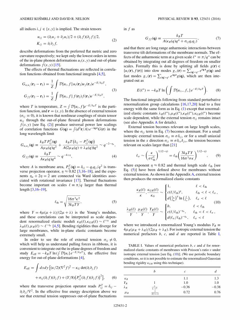
TABLE I. Values of numerical prefactors b, c and d for renor-malized elastic constants of membranes with Poisson’s ratio ν underisotropic external tension [see Eq. (10)]. (We use periodic boundaryconditions, so it is not possible to estimate the renormalized Gaussianbending rigidity κGR using this technique).

b c d

κR 1.1 1.3YR 1 1.0 1.0λR

ν

1−ν2 −0.36 −0.38

μR1

2(1+ν) 0.72 0.76

125431-2

RESPONSE OF THERMALIZED RIBBONS TO PULLING . . . PHYSICAL REVIEW B 93, 125431 (2016)

/ th10-2 10-1 100 101 102 103 104 105 106 107 108 109

-0.4

-0.3

-0.2

-0.1

0

0.1

0.2

/ th10-2 10-1 100 101 102 103 104 105 106 107 108 10910-3

10-210-1100101102103104105106

κR( )/κYR( )/Y

< th th < < σ σ <

< th th < < σ σ <

(a)

(b)

∼th

+η

∼th

−ηu

∼ σ

th

+η

lnσ

∼ σ

th

−ηu

νR( ) ≡ λR( )(2μR( ) + λR( ))

FIG. 1. Renormalization of elastic constants (a) and the Pois-son’s ratio (b) for membranes under small isotropic tension. Wechose parameters suitable for the graphene membrane at roomtemperature: κ = 1.1 eV, Y = 340 N/m, ν = λ/(2μ + λ) = 0.156,σ = 10−7 N/m, �th ≈ 2 nm, �σ /�th ≈ 3 × 105.

and Fig. 1 displays the scale dependent renormalized elasticconstants, where the three regimes presented in Eq. (10)become evident. The uniaxial external tension produces similarrenormalized elastic constants, but with slightly differentnumerical prefactors d, while prefactors b and c remain thesame (see Appendix A).

The renormalized elastic constants can also be used todefine the renormalized Poisson’s ratio

νR(�) ≡ λR(�)

2μR(�) + λR(�)={

λ2μ+λ

, � < �th

− 13 , �th < �

. (11)

At short length scales (� < �th) there is no renormalizationand the Poisson’s ratio is set by the material, while atlarge length scales (� > �th) the renormalized Poisson’s ratioapproaches the universal value of −1/3 (see Fig. 1). Theuniversal negative Poisson’s ratio was first predicted by theself consistent scaling analysis [18], which was confirmed byMonte Carlo simulations [22] of membranes without externaltension (σij ≡ 0).

For sufficiently large external tension σ � kBT Y/κ ≡σ ∗ [21], which corresponds to �th � �σ , thermal fluctuationsbecome irrelevant and the renormalized elastic constants are

approximately equal to the microscopic ones. Remarkably,for graphene membranes with κ = 1.1 eV [23] and Y =340 N/m [24], the thermal length at room temperature is oforder several graphene lattice constants, �th ∼ 2 nm [5,13].Therefore thermal fluctuations are important for essentially allroom temperature graphene experiments, provided only thatthe external membrane tension is smaller than σ ∗ ∼ 10 N/m.

Note that the out of plane correlation function becomesG−1

ff (q) = AkBT

[κR(q) q4 + σij qiqj ], where the renormalizedbending rigidity is set by Eq. (10). For isotropic externaltensions this result agrees with Roldan et al., [21] but the resultsfor uniaxial external tension appear to be new. With a uniaxialtension, the long wavelength f (q) fluctuations behave like thelayer displacements of a defect-free two-dimensional smecticliquid crystal [25], with fluctuations along the direction x ofthe pulling force having a reduced amplitude

G−1ff

(|q| < �−1σ

) ∼ A

kBT

[σq2

x + κqy4(�σ /�th)η

]. (12)

The cutoff of renormalized elastic constants due to externaltension is also responsible for the nonlinear stretching of largemembranes of size L as we demonstrate below. In the absenceof external tension the projected membrane area shrinks dueto thermal fluctuations as⟨

δA

A

⟩0

≈ −1

2

∑q

q2Gff (q),

(13)⟨δA

A

⟩0

≈ −kBT

4πκ

[1

η+ ln

(�th

a0

)],

where a0 is a microscopic cutoff (e.g., the graphene latticeconstant), and this reflects a negative coefficient of thermalexpansion

α = 1

A

dA

dT≈ − kB

4πκ

[1

η− 1

2+ ln

(�th

a0

)]. (14)

In the presence of isotropic external tension the change inprojected membrane area is expressed as⟨

δA

A

⟩≈ σ

(μ + λ)− 1

2

∑q

q2Gff (q), (15)

where the first term describes stretching of material and thesecond term describes shrinking due to thermal fluctuations.For infinitesimally small isotropic external tension (σ κR(L)/L2) there is no cutoff for the renormalization of elasticconstants (L �σ ) and the projected area increases as⟨

δA

A

⟩≈⟨δA

A

⟩0

+ B σ

Y

(L

�th

)ηu

, (16)

where B ≈ 2.3. Due to the renormalization the effective bulkmodulus (≈YR(L)) is much smaller then the material bulkmodulus (μ + λ). For larger isotropic external tension (σ �κR(L)/L2) the cutoff of renormalized elastic constants (�σ L) produces⟨

δA

A

⟩≈⟨δA

A

⟩0

+ C kBT

κ

(κσ

kBT Y

)η/(2−η)

+ σ

(μ + λ), (17)

where C ≈ 1.2. The second term describes the nonlinearstretching for small uniform tension σ in the presence of

125431-3

ANDREJ KOSMRLJ AND DAVID R. NELSON PHYSICAL REVIEW B 93, 125431 (2016)

σκ/(kBTY )10-1010-9 10-8 10-7 10-6 10-5 10-4 10-3 10-2 10-1 100 101 102 103

δA/A

−δA

/A0

10-1010-910-810-710-610-510-410-310-210-1100101102

L < σ(σ) th < σ(σ) < L σ(σ) < th

∼ σ

(μ + λ)

∼ σ

YR(L)

∼ ση/(2−η) ∼ σ0.7

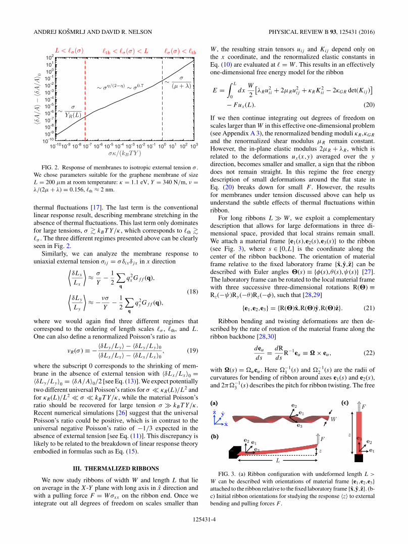
FIG. 2. Response of membranes to isotropic external tension σ .We chose parameters suitable for the graphene membrane of sizeL = 200 μm at room temperature: κ = 1.1 eV, Y = 340 N/m, ν =λ/(2μ + λ) = 0.156, �th ≈ 2 nm.

thermal fluctuations [17]. The last term is the conventionallinear response result, describing membrane stretching in theabsence of thermal fluctuations. This last term only dominatesfor large tensions, σ � kBT Y/κ , which corresponds to �th ��σ . The three different regimes presented above can be clearlyseen in Fig. 2.

Similarly, we can analyze the membrane response touniaxial external tension σij = σδixδjx in x direction⟨

δLx

Lx

⟩≈ σ

Y− 1

2

∑q

q2xGff (q),

(18)⟨δLy

Ly

⟩≈ −νσ

Y− 1

2

∑q

q2yGff (q),

where we would again find three different regimes thatcorrespond to the ordering of length scales �σ , �th, and L.One can also define a renormalized Poisson’s ratio as

νR(σ ) ≡ −〈δLy/Ly〉 − 〈δLy/Ly〉0

〈δLx/Lx〉 − 〈δLx/Lx〉0, (19)

where the subscript 0 corresponds to the shrinking of mem-brane in the absence of external tension with 〈δLx/Lx〉0 =〈δLy/Ly〉0 = 〈δA/A〉0/2 [see Eq. (13)]. We expect potentiallytwo different universal Poisson’s ratios for σ κR(L)/L2 andfor κR(L)/L2 σ kBT Y/κ , while the material Poisson’sratio should be recovered for large tension σ � kBT Y/κ .Recent numerical simulations [26] suggest that the universalPoisson’s ratio could be positive, which is in contrast to theuniversal negative Poisson’s ratio of −1/3 expected in theabsence of external tension [see Eq. (11)]. This discrepancy islikely to be related to the breakdown of linear response theoryembodied in formulas such as Eq. (15).

III. THERMALIZED RIBBONS

We now study ribbons of width W and length L that lieon average in the X-Y plane with long axis in x direction andwith a pulling force F = Wσxx on the ribbon end. Once weintegrate out all degrees of freedom on scales smaller than

W , the resulting strain tensors uij and Kij depend only onthe x coordinate, and the renormalized elastic constants inEq. (10) are evaluated at � = W . This results in an effectivelyone-dimensional free energy model for the ribbon

E =∫ L

0dx

W

2

[λRu2

ii + 2μRu2ij + κRK2

ii − 2κGR det(Kij )]

−Fux(L). (20)

If we then continue integrating out degrees of freedom onscales larger than W in this effective one-dimensional problem(see Appendix A 3), the renormalized bending moduli κR,κGR

and the renormalized shear modulus μR remain constant.However, the in-plane elastic modulus 2μR + λR , which isrelated to the deformations ux(x,y) averaged over the y

direction, becomes smaller and smaller, a sign that the ribbondoes not remain straight. In this regime the free energydescription of small deformations around the flat state inEq. (20) breaks down for small F . However, the resultsfor membranes under tension discussed above can help usunderstand the subtle effects of thermal fluctuations withinribbon.

For long ribbons L � W , we exploit a complementarydescription that allows for large deformations in three di-mensional space, provided that local strains remain small.We attach a material frame {e1(s),e2(s),e3(s)} to the ribbon(see Fig. 3), where s ∈ [0,L] is the coordinate along thecenter of the ribbon backbone. The orientation of materialframe relative to the fixed laboratory frame {x,y,z} can bedescribed with Euler angles �(s) ≡ {φ(s),θ (s),ψ(s)} [27].The laboratory frame can be rotated to the local material framewith three successive three-dimensional rotations R(�) ≡Rz(−ψ)Ry(−θ )Rz(−φ), such that [28,29]

{e1,e2,e3} = {R(�)x,R(�)y,R(�)z}. (21)

Ribbon bending and twisting deformations are then de-scribed by the rate of rotation of the material frame along theribbon backbone [28,30]

deα

ds= dR

dsR−1eα ≡ � × eα, (22)

with �(s) = �αeα . Here �−11 (s) and �−1

2 (s) are the radii ofcurvatures for bending of ribbon around axes e1(s) and e2(s),and 2π�−1

3 (s) describes the pitch for ribbon twisting. The free

z

x

y

(a)

(b)

(c)

=⇒F

z

e3

e1

e2

e1

e2e3

z

e2 e1

e3

=⇒F

L

W

FIG. 3. (a) Ribbon configuration with undeformed length L >

W can be described with orientations of material frame {e1,e2,e3}attached to the ribbon relative to the fixed laboratory frame {x,y,z}. (b-c) Initial ribbon orientations for studying the response 〈z〉 to externalbending and pulling forces F .

125431-4

RESPONSE OF THERMALIZED RIBBONS TO PULLING . . . PHYSICAL REVIEW B 93, 125431 (2016)

energy cost of a ribbon deformation is then [28–30]

E =∫ L

0ds

1

2

[A1�

21 + A2�

22 + C�2

3 + ku233

]− F · r(L),

(23)where A1, A2 are bending rigidities, C is torsional rigidity, k isstiffness, u33 is local strain along the ribbon tangent, and F isthe applied force on a ribbon end at r(L), which can representeither bending or pulling (see Fig. 3). From comparison withthe effective one-dimensional ribbon model in Eq. (20) we find

A1 = WκR(W ), C = 2WκGR(W ), k = WYR(W ), (24)

where renormalized constants are defined in Eq. (10). Thesecond bending rigidity for splay around axis e2(s), involvesribbon stretching and is much larger; in fact, A2’s barevalue exceeds A1 and C by a large factor of order YW 2/κ .We expect κG ∼ κ for graphene both microscopically [15]and when thermal renormalizations are accounted for. Bymapping onto classical zero temperature solid mechanicswe find A2 ∼ W 3YR(W ) [15]. For ribbons whose width ismuch larger than it’s thickness we thus have A2 � A1,C

and we can set �2 ≈ 0. We also neglect the stretching ofribbon backbone (u33 ≈ 0), as is appropriate when the pullingforce resisting entropic contraction is not too large [31]. Theeffective one-dimensional free energy model presented abovecorresponds to the highly asymmetric 1d polymer [28–30],with anomalous W -dependent elastic parameters.

The response 〈z〉 of the ribbon to external force F in the zdirection can be evaluated from the relation [31]

〈z〉 = kBT (∂ ln Z/∂F ), (25)

where the partition function reads Z = ∫D[�(s)]e−E/kBT .

Note that we can study both pulling and bending forces, wherethe only difference is the Euler angles embodied in the initialorientation of ribbon (see Fig. 3). If we clamp the ribbon atthe origin (s = 0) and apply force on the ribbon end (s = L),then for pulling the initial condition is �i = {0,0,0}. To treatbending, we consider a ribbon initially aligned with the x axisand take �i = {π/2,π/2,0}.

To evaluate the partition function Z, it is convenient todefine the unnormalized probability distribution ρ(�,s) ofEuler angles � at a contour length s along the ribbon midlineas

ρ(�f ,sf ) =∫ �(s=sf )=�f

�(s=0)=�i

D[�(s)]e−E/kBT , (26)

where the path integral above is restricted to s ∈ [0,sf ] andthe partition function is given by Z = ∫

d�ρ(�,L) with

the Euler-angle measure∫

d� ≡ ∫ 2π

0 dφ∫ π

0 sin θdθ∫ 2π

0 dψ .The evolution of this probability distribution along the ribbonbackbone is described with differential equation [28,32](

∂

∂s+ H

)ρ(�,s) = 0, (27)

where the Hamiltonian operator is

H = kBT

2

(J 2

1

A1+ J 2

2

A2+ J 2

3

C

)− F (e3 · z)

kBT. (28)

Here the {Jα} are angular momentum operators around axeseα , which can be expressed in terms of derivatives with respect

to Euler angles [27,32]. As shown in Appendix B the evolutionof ρ(�,s) with s maps the physics of thermalized ribbons ontothe Schrodinger equation of the asymmetric rotating top in anexternal gravitational field [27], where the ribbon backbonecoordinate s plays a role of imaginary time and the bendingand twisting rigidities A1, A2, and C correspond to momentsof inertia. The evolution of the material frame orientationdistribution can be evaluated by expanding the initial conditionin eigen-distributions,

ρ(�,0) = δ(� − �i) =∑

a

Caρa(�), (29)

where Hρa(�) = λaρa(�). In this decomposition the parti-tion function becomes

Z =∑

a

Cae−λaL

∫d�ρa(�) (30)

and the response 〈z〉 to an external force can be evaluated fromZ as described above [see Eq. (25)].

To treat ribbons in both the semiflexible and highly crum-pled regimes, we must find all eigenvalues of the Hamiltonianoperator λa and eigendistributions ρa(�). From quantummechanics we know that this is done efficiently in the basis ofWigner D functions [27] D

j

mk(�), which have well definedquantum numbers j,k,m for the total angular momentumJ 2 = J 2

1 + J 22 + J 2

3 , the angular momentum around the ribbontangent J3, and for the angular momentum around the labora-tory axis Jz. For details see Refs. [28,32] and the Appendix B.

With the help of this machinery we first studied theresponse of ribbons of various lengths to small external pullingand bending forces at fixed temperature (see Fig. 4). Here,since C and A1 have a similar order of magnitude, we takeC = A1, for simplicity. Similar to single molecule polymerphysics [33,34], we find two regimes. For ribbons much shorterthan a persistence length [29]

�p = 2

kBT(A−1

1 + A−12

) ≈ 2WκR(W )

kBT. (31)

FIG. 4. Pulling and bending deflections 〈z/L〉 of ribbons withbending rigidities A2/A1 → ∞ and twisting rigidity C/A1 = 1 inresponse to a fixed small external force FA1/(kBT )2 = 0.01. Theslope of +2 for bending when L �p agrees with expectations forstiff cantilevers with, however, a bending rigidity greatly enhanced bya factor (W/�th)η � 1. The responses to pulling and bending forcesagree when L � �p .

125431-5

ANDREJ KOSMRLJ AND DAVID R. NELSON PHYSICAL REVIEW B 93, 125431 (2016)

FIG. 5. Response of ribbons (neglecting quantum fluctuations) toa small bending force at various temperatures for fixed W , L, F , κ ,and Y . Three regimes appear for the parameter choices, FL2/3Wκ =0.01, YW 2/κ = 105, L/W = 102.

ribbons behave like stiff “classical rods” [15], where forpulling 〈z〉 ≈ L and for the bending (cantilever) mode 〈z〉 =FL3/3A1. Note that A−1

2 is negligible and that thermalfluctuations on scales less than W lead to a renormalizedbending rigidity A1 [see Eq. (24)], orders of magnitude largerthan for rod-like polymers at room temperature, as foundby the Cornell experiments [13]. For ribbons much longerthan the persistence length (L � �p), pulling and bendingbecome equivalent. In this semi-flexible regime ribbon forgetsits initial orientation after a persistence length, and for smallpulling forces the response to either bending or pulling is〈z/L〉 = 2F�p/(3kBT ) [2]. Eventually, at much larger ribbonlengths than those considered here, ribbon self-avoidance willbecome important [31].

To highlight the difference between conventional polymersand thermalized ribbons with W � �th, consider the responseof ribbons to a small bending force, FL2/Wκ 1. Figure 5shows results for a wide variety of temperatures, obtainedby inserting temperature dependences hidden in A1 and�p. We find three distinct regimes: At low temperatures,where W �th ∼ κ/

√kBT Y , thermal fluctuations are neg-

ligible and ribbon behaves like a classic cantilever withbare elastic parameters, 〈z〉 = FL3/(3κW ). As the temper-ature increases, the thermal length scale drops and eventuallybecomes smaller than the ribbon width (�th W ). In thisregime the renormalized bending rigidity is increased due tothermal fluctuations and the cantilever deflection is smaller〈z〉 ≈ FL3�

η

th/(3κW 1+η) ∼ T −η/2. As temperature increaseseven further, eventually the persistence length �p becomessmaller than the ribbon length L. As noted above in thissemi-flexible regime the deflection now becomes 〈z〉 ≈4κFLW 1+η/(3(kBT )2�

η

th) ∼ T −(2−η/2) and drops even fasterwith temperature, as the ribbon transforms from a cantileverinto a random coil. Note that with rising temperatures the cutofflength scale �σ associated with ribbon tension [see Eq. (9)] alsoincreases, but never becomes relevant.

However, ribbons with large pulling forces neverthelessshow a nontrivial response due to the cutoff �σ . For largepulling forces, F�p � kBT , we also need to include thestretching of the ribbon backbone, with the result similar to

FIG. 6. Contributions of backbone stretching (blue line) andentropic elasticity (dashed black line) to 〈z/L〉, describing theresponse to large ribbon pulling forces. We chose parameterskBT /κ = 1/40 (suitable for graphene at room temperature), andW/�th = 104 (200 μm width ribbon at room temperature).

Ref. [28] (see also Appendix B)⟨z

L

⟩≈ −kBT

8πκ

[1

η+ ln

(�th

a0

)]+ F

k− kBT

4√

FA1, (32)

where a0 is a microscopic cutoff (e.g., the graphene latticeconstant) and k = WYR(W ) is the effective one-dimensionalribbon stiffness. The first term describes shrinking due tothermal fluctuations within the ribbon, the middle termdescribes stretching of the ribbon backbone, and the finalcorrection corresponds to the entropic contribution fromribbon fluctuations. As F = σW increases the cutoff lengthscale �σ [Eq. (9)] drops and we find two crossovers, first whenthis length scale crosses the ribbon width W and finally when itdrops below the thermal length scale �th (see Fig. 6). Especiallyinteresting is the nonlinear intermediate force regime with�th �σ W , where we find that the ribbon backbonestretches as F/k ∼ Fη/(2−η), which generalizes to ribbons thenonlinear stretching result [Eq. (17)] to uniaxial pulling.

IV. CONCLUSIONS

For graphene ribbons, where �th ≈ 2 nm at room temper-ature, the experiments of Blees et al. [13] on ribbons ofwidth W = 10 μm, confirmed a renormalized bending rigidityκR(W )/κ ∼ 4000, consistent with Eq. (10). The correspondingpersistence length is of order of meters. Thus �p � L forgraphene ribbons of lengths L ∼ 10–100 μm, which shouldbehave like conventional cantilevers with, however, a stronglyrenormalized L independent bending rigidity. Probing thesemi-flexible regime requires narrower ribbons of order 10nanometers width, so that the persistence length should be inthe experimentally accessible regime of 1–10 micrometers.Although the value of the critical pulling tension, beyondwhich thermal fluctuations become irrelevant, is F/W =σ ∗ ∼ 10 N/m for graphene, one could observe interestingbehavior for smaller tensions where �th < �σ < W .

Additional novel behavior can arise for free-standing sheetsat sufficiently high temperatures even when L ≈ W . Tosee this, consider the correlation function of the membrane

125431-6

RESPONSE OF THERMALIZED RIBBONS TO PULLING . . . PHYSICAL REVIEW B 93, 125431 (2016)

normals n(x,y) = (−∂xf,−∂yf,1)/√

1 + |∇f |2 that definesthe flat phase [3]. There is a power law approach to longrange order, 〈n(ra) · n(rb)〉 = 1 − kBT

2πκ[η−1 + ln(�th/a0)] +

C kBTκ

( �th|ra−rb | )

η, where C is a positive constant of order unity and

a0 is microscopic cutoff, of order the graphene lattice spacing(see Appendix A 1, which includes the effect of an isotropicexternal stress). The second term represents the reductionin the long range order due to thermal fluctuations. Whenthis term becomes the same size as the first (i.e. for kBT �2πκη), the low temperature flat phase can transform into aentropically dominated crumpled ball, with a size limited byself-avoidance, provided monolayer sheets such as graphenemaintain their integrity [19]. The transition temperature toisotropic crumpling could be lowered by creating a graphenesheet with a periodic array of holes or cuts. (Althoughcuts could be deployed with equal numbers at 120 degreeangles, an array of parallel cuts could lead to a system thatis crumpled in one direction, but tube-like in another, asituation studied theoretically in Ref. [35].) While we havesome understanding of force-free conformations [36], littleis known about the mechanical properties of free-standingmembranes at or above this crumpling transition. There isevidence from computer simulations of a high temperaturecompact phase, where attractive van der Waals interactionsare balanced by self-avoidance [37]. We hope this paper willstimulate further investigations on these problems in the spiritof single-molecule experiments on linear polymers [33,34].

ACKNOWLEDGMENTS

We acknowledge support by the National Science Founda-tion, through grants DMR1306367 and DMR1435999, andthrough the Harvard Materials Research and EngineeringCenter through Grant DMR1420570. We would also like toacknowledge conversations with P. McEuen, M. Blees, M.Bowick and R. Sknepnek.

APPENDIX A: RENORMALIZATION GROUPTREATMENT OF MEMBRANES UNDER TENSION

Our goal is to analyze properties of fluctuating membranesunder external tension σij with the renormalization groupapproach. The free energy cost of membrane deformationsunder tension is

E =∫

d2x1

2

[λu2

ii + 2μu2ij + κK2

ii − 2κG det(Kij )]

−∮

ds miσijuj , (A1)

where uij = (∂iuj + ∂jui + ∂if ∂jf )/2 is the nonlinear straintensor, Kij = ∂i∂jf is the bending strain tensor, the ui arein-plane deformations, f is the out-of-plane deformation, andmi describes a normal vector to the membrane boundary. Usingthe divergence theorem we can convert the boundary work termto the area integral, such that the free energy becomes

E =∫

d2x(

1

2

[λu2

ii + 2μu2ij + κK2

ii − 2κG det(Kij )]− σiju

0ij

), (A2)

where u0ij = (∂iuj + ∂jui)/2 is the linear part of the strain tensor. Since the in-plane deformations ui only appear quadratically

in [Eq. (A2)], we can integrate them out to derive the effective free energy for the out-of-plane deformations [4],

Eeff

A=∑

q

1

2[κq4 + σij qiqj ]f (q)f (−q) +

∑q1 + q2 = q �= 0

q3 + q4 = −q �= 0

Y

8

[q1iP

Tij (q)q2j

][q3iP

Tij (q)q4j

]f (q1)f (q2)f (q3)f (q4), (A3)

where the Young’s modulus is Y = 4μ(μ + λ)/(2μ + λ), the projection operator P Tij (q) = δij − qiqj /q

2, A is the membrane areaand the Fourier modes are f (q) = ∫

(d2r/A)e−iq·rf (r). From the expression above we can clearly see that positive componentsof the membrane tension σij constrain the out-of-plane fluctuations f .

To implement a momentum shell renormalization group, we first integrate out all Fourier modes in a thin momentum shell�/b < q < �, where � is microscopic cutoff and b ≡ �� = es with s 1. Next we rescale lengths and fields [16,38]

x = bx′, f (x) = bζf f ′(x′). (A4)

We find it convenient to work directly with a D = 2 dimensional membrane embedded in d = 3 space, rather than introducingan expansion in ε = 4 − D [16]. Finally, we define new elastic constants κ ′, Y ′, and external tension σ ′

ij , such that the freeenergy functional in Eq. (A3) retains the same form after the first two renormalization group steps. It is common to introduce β

functions [20], which define the flow of elastic constants

βκ = ∂κ ′

∂ ln b= 2(ζf − 1)κ + Zκ ≡ ∂κ ′

∂s,

βY = ∂Y ′

∂ ln b= 2(2ζf − 1)Y + ZY ≡ ∂Y ′

∂s, (A5)

βij = ∂σ ′ij

∂ ln b= 2ζf σij ≡ ∂σ ′

ij

∂s.

125431-7

ANDREJ KOSMRLJ AND DAVID R. NELSON PHYSICAL REVIEW B 93, 125431 (2016)

Above we introduced Z functions, which result from the integrals of modes over the momentum shell. To one loop order (seeFig. 7), the Z functions read

Zκ = + ∂

∂ ln b

⎛⎝Y

∑�b<p<�

(1 − (q · p)2)2〈f (p)f (−p)〉⎞⎠,

(A6)

ZY = − ∂

∂ ln b

⎛⎝ Y 2A

2kBT

∑�b<p<�

(1 − (q · p)2)2p4〈f (p)f (−p)〉2

⎞⎠,

where � is the microscopic momentum cutoff and A is theundeformed membrane area. Note that the only change in thestress tensor σij to this order arises from the rescaling factor ζf .Upon assuming that the initial membrane tension σij is small,such that σij κ�2, then 〈f (p)f (−p)〉 ≈ kBT /(Aκp4) inequations above and the β functions in one loop approximationbecome

βκ = 2(ζf − 1)κ + 3YkBT

16πκ�2,

βY = 2(2ζf − 1)Y − 3Y 2kBT

32πκ2�2, (A7)

βij = 2ζf σij .

It is convenient to chose ζf such that βκ = 0, which results inζf = 1 − 3YkBT

32πκ2�2 , and

βY = 2Y − 15Y 2kBT

32πκ2�2,

(A8)

βij = 2

(1 − 3YkBT

32πκ2�2

)σij .

By repeating the renormalization group procedure, we inte-grate out modes at the smallest length scale and evolve theYoung’s modulus Y and external tension σij . Initially, theyboth grow rapidly

Y (�) ≈ Y × (��)2,(A9)

σij (�) ≈ σij × (��)2,

where we integrated out all modes on scales smaller than�. Once we integrate out all modes up to the scale �th ∼κ/

√kBT Y Young’s modulus reaches a fixed point

Y ∗ = 64πκ2�2

15kBT∼ Y × (�th�)2. (A10)

q q

p(a) (b)

q q

p

q − pq − p

FIG. 7. One loop corrections to the renormalization of (a) κ

and (b) Y . Solid lines represent propagators for the out-of-planedisplacements f (q) and dashed lines represent the momentum carriedby the vertex Y .

At the fixed point we introduce the exponent η, such thatζf = 1 − η/2. Note that ζf ≈ 1 initially, before we reachthe fixed point. In the one loop approximation we findη = 4/5, which approximates the value of η ≈ 0.82 obtainedby the self-consistent screening approximation [18] and η ≈0.85 obtained by the nonperturbative renormalization groupcalculations [39]. This result differs from a formal one loopε = 4 − D expansion, which results in η = 12ε/25 [16],because we have performed the one loop calculations directlyfor D = 2 dimensional membranes, rather than calculatingthem for small ε, i.e. for D ≈ 4 dimensional membranes.

By continuing with the renormalization group procedureand integrating out modes beyond the scale �th, we find thatthe initially small membrane tension now grows as

σij (� > �th) = σij × (�/�th)2−η × (�th�)2. (A11)

Eventually, the membrane tension becomes large enough thatit becomes important. This happens at the scale

�σ ∼(

κ

σ�η

th

)1/(2−η)

, (A12)

when σij (�σ ) ∼ κ�2. At this stage, we have to take into ac-count the membrane tension, when evaluating the Z functionsin Eq. (A6). In next subsections, we describe what happens formembranes under various external tension conditions. We firstdiscuss membranes with W ∼ L, and then move on to discussribbons with L � W .

1. Membranes under uniform tension

We first consider membranes under uniform tension σij =σδij . After integrating modes on scales smaller than �σ , themembrane tension becomes relevant and beyond this point wecan approximate 〈f (p)f (−p)〉 ≈ kBT /(Aσp2) in Eq. (A6).With this change, the β functions become

βκ = 2(ζf − 1)κ + 3YkBT

16πσ,

βY = 2(2ζf − 1)Y − 3Y 2kBT �2

32πσ 2, (A13)

βij = 2ζf σij .

It is now convenient to set ζf = 0 so that the uniform tensionremains unchanged. We then find that both the bending rigidityκ and the Young’s modulus Y flow to 0 at large length scales,

κ(� > �σ ) ∼ κ × (�/�σ )−2,(A14)

Y (� > �σ ) ∼ Y ∗ × (�/�σ )−2.

125431-8

RESPONSE OF THERMALIZED RIBBONS TO PULLING . . . PHYSICAL REVIEW B 93, 125431 (2016)

In this regime the external tension dominates and thermalfluctuations are unimportant. After rescaling lengths and fieldsback to the initial units we find the renormalized elasticconstants

κR(�)

κ∼

⎧⎪⎨⎪⎩

1, � < �th

(�/�th)η, �th < � < �σ(�σ

�th

)ηln(

��σ

), �σ < �

,

YR(�)

Y∼

⎧⎪⎨⎪⎩

1, � < �th

(�/�th)−ηu , �th < � < �σ

(�σ /�th)−ηu , �σ < �

, (A15)

and the height correlation function for out-of-plane flexuralphonons is

〈f (q)f (−q)〉 ≡ kBT

A(σq2 + κR(q)q4), (A16)

where q = π/�.By performing similar analysis with the initial free energy

model [see Eq. (A2)] we can also analyze the flow of elastic

constants λ and μ as

βκ = 2(ζf − 1)κ + 3YkBT

16π (σ + κ�2),

βY = 2(2ζf − 1)Y − 3Y 2kBT �2

32π (σ + κ�2)2,

βμ = 2(2ζf − 1)μ − μ2kBT �2

8π (σ + κ�2)2, (A17)

βλ = 2(2ζf − 1)λ − [μ2 + 4μλ + 2λ2]kBT �2

8π (σ + κ�2)2,

βij = 2ζf σij ,

and we find that the renormalized constants λR(�) and μR(�)behave similarly as the renormalized Young’s modulus YR(�)in Eq. (A15). This set of differential equations was also usedto produce Fig. 1.

Finally, we present the correlation function of the mem-brane normals n(x,y) = (−∂xf,−∂yf,1)/

√1 + |∇f |2 that

defines the flat phase [3]. When deformations are small the cor-relation function of the membrane normals is approximately

〈n(ra) · n(rb)〉 ≈ 1 −∑

q

q2[1 − eiq·(ra−rb)]〈|f (q)|2〉. (A18)

For small tension σ � kBT Y/κ this correlation functionevaluates to

〈n(ra) · n(rb)〉 ≈ 1 − kBT

(2πκ)[η−1 + ln(�th�)] + kBT

(2πκ)(η−1 − 2−1)

(κσ

kBT Y

)η/(2−η)

+ kBT

κ

{C(

�th|ra−rb|

)η, �th |ra − rb| �σ

D(

�th�σ

)ηe−|ra−rb|/�σ , �σ |ra − rb|

, (A19)

where C = 12π

∫∞0

dxx1−η J0(x) ≈ 0.2, D is another constant

of order unity and J0(x) is the Bessel function of the firstkind. The second term in the equation above represents thereduction in the long range order between normals due tothermal fluctuations and the third term shows how this longrange order is restored with external tension. For large tensionσ � kBT Y/κ , where the effects of thermal fluctuations aresuppressed, we find

〈n(ra) · n(rb)〉 ≈ 1 − kBT

(4πκ)ln

[1 + κ�2

σ

]

+ kBT

(2πκ)K0(|ra − rb|

√σ/κ), (A20)

where K0(x) is the modified Bessel function of the secondkind, which asymptotically scales as K0(x) � √

π/(2x)e−x .Note that the nonlinear dependence of the membrane

extension 〈u0ii〉 = 〈δA/A〉 on the external tension σ presented

in Eq. (17) can be obtained simply from the scaling arguments.Since the external tension σ is a conjugate variable to ∂jui ,their rescalings are connected. Once we rescale lengths as x =bx ′ and in-plane deformations ui = bζuu′

i , then the externaltension rescales as σ = bζσ σ ′ with ζσ = 1 − D − ζu, whereD = 2 is the membrane dimensionality. We also know that the

Ward identities associated with rotational symmetry connectrescaling of the in-plane and out-of-plane deformations suchthat ζu = 2ζf − 1 and therefore ζσ = −2ζf [17]. As men-tioned above we can extract exponent η from ζf = 1 − η/2,which leads to ζu = 1 − η and ζσ = −2 + η. Now we haveall necessary ingredients to calculate the scaling of membraneextension as⟨

δu0ii(σ )

⟩ = ⟨δu0

ii

′(σ ′)

⟩bζu−1 = ⟨

δu0ii(σb−ζσ )

⟩bζu−1. (A21)

Since the rescaling factor b is arbitrary, we can pick b = σ 1/ζσ

to find⟨δu0

ii(σ )⟩ = ⟨

δu0ii(1)

⟩σ (ζu−1)/ζσ = const. × ση/(2−η). (A22)

Thus we found the same nonlinear scaling between themembrane stretching and the uniform tension as in Eq. (17),which holds for small uniform tension.

2. Membranes under uniaxial tension

In this section we consider membranes under uniaxialtension σxx > 0, while σyy = σxy = 0. Upon again integrat-ing out modes on scales smaller than �σ , the membranetension becomes important and beyond this point we haveto take 〈f (p)f (−p)〉 ≈ kBT /[A(σxxp

2x + κp4

y)] in Eq. (A6).

125431-9

ANDREJ KOSMRLJ AND DAVID R. NELSON PHYSICAL REVIEW B 93, 125431 (2016)

Although we can ignore a term κ(p4x + 2p2

xp2y) compared to

σxxp2x , we have to keep the term with κp4

y . Once we integrateout modes from a thin shell �/b < p < �, we find that thequadratic term in the free energy becomes

1

2

∑q

f (q)f (−q)

{σxxq

2x + κq4

y + YkBT ln b

4π

×[

2q4x

�√

κσxx

+ 1

σxx

(−3q4x + 6q2

xq2y + q4

y

)]}. (A23)

All new generated terms that involve qx are negligiblecompared to the σxxq

2x . Therefore we can keep only the last

term with q4y to calculate the βκ function that renormalizes the

bending rigidity,

βκ = 2(ζf − 1)κ + YkBT

4πσxx

. (A24)

For the quartic term with momentum-dependent Young’smodulus Y we find that after the momentum shell integrationthere are again anisotropic contributions in terms of qx andqy . Significantly, all renormalizations of Y are negative and β

functions now take the form

βκ = 2(ζf − 1)κ + YkBT

4πσxx

,

βY = 2(2ζf − 1)Y − Y 2kBT �2

4πσ 2xx

, (A25)

βij = 2ζf σij .

As for the uniform tension case, we choose ζf = 0 to fix theuniaxial tension, and find that both the bending rigidity κ andthe Young’s modulus Y again flow to 0 as

κ(� > �σ ) ∼ κ × (�/�σ )−2,(A26)

Y (� > �σ ) ∼ Y ∗ × (�/�σ )−2.

After rescaling lengths and fields back to the initial units wefind that the renormalized elastic constants scale similarlyas for the uniform external tension [see Eq. (A15)] andthe correlation function for the out-of-plane deformationsbecomes highly anisotropic

〈f (q)f (−q)〉 = kBT

A[σxxq2

x + κR(q)q4] , (A27)

where q = π/�. We can now use this result to calculate themembrane strains associated with uniaxial stretching

〈δLx/Lx〉 = σxx

Y− 1

2

∑q

q2x 〈f (q)f (−q)〉,

〈δLx/Lx〉 ≈ −kBT

8πκ[η−1 + ln(�th�)] + kBT

8πκ[η−1 − 1 +

√2 − sinh−1(1)]

(κσxx

kBT Y

)η/(2−η)

+ σxx

Y,

(A28)

〈δLy/Ly〉 = −νσxx

Y− 1

2

∑q

q2y 〈f (q)f (−q)〉,

〈δLy/Ly〉 ≈ −kBT

8πκ[η−1 + ln(�th�)] + kBT

8πκ[η−1 + 1 −

√2 − sinh−1(1)]

(κσxx

kBT Y

)η/(2−η)

− νσxx

Y,

where ν = λ/(2μ + λ) is the two-dimensional Poisson ratio.The first terms in the second and fourth lines describemembrane shrinkage due to thermal fluctuations, the secondterms correspond to nonlinear membrane stretching in thepresence of thermal fluctuations, and the last terms correspondto the zero temperature response, which becomes relevant forσxx � kBT Y/κ . The power law scalings above are accurate,but the numerical prefactors are approximate. In order tocalculate numerical prefactors exactly, we would need toknow how the correlation function in Eq. (A27) behaves intransition regions. In principle, the renormalized Poisson’sratio is calculated as

νR = −〈δLy/Ly〉 − 〈δLy/Ly〉0

〈δLx/Lx〉 − 〈δLx/Lx〉0, (A29)

where the subscript 0 describes the membrane shrinking in theabsence of external tension (σxx ≡ 0). Because our numericalprefactors in Eq. (A28) are just approximate we cannotdetermine the precise value of the renormalized Poisson’s ratioνR in the regime dominated by thermal fluctuations, but we

know that the νR transitions to the zero temperature value ν

for large pulling tension, i.e., σxx � kBT Y/κ .

3. Pulling of ribbons

Finally, we comment on pulling on large aspect ratioribbons of length L and width W L. After integrating outall degrees of freedom on scales smaller than the width W ,the resulting strain tensors uij and Kij depend only on the x

coordinate and the renormalized elastic constants are evaluatedat q = π/W . This results in an effectively one-dimensionalfree energy model for the ribbon

E =∫ L

0dx W

(1

2λRu2

ii + μRu2ij + 1

2κRK2

ii

− κGR det(Kij ) − σxxu0xx

). (A30)

It is convenient to rewrite the effective free energy abovein terms of one-dimensional Fourier variables s(q) ≡∫

(dx/L)e−iqxs(x) and to separate out the uniform strain

125431-10

RESPONSE OF THERMALIZED RIBBONS TO PULLING . . . PHYSICAL REVIEW B 93, 125431 (2016)

u0ij [4]. The resulting free energy reads

E

WL= 1

2

[λR

(u0

ii

)2 + 2μR

(u0

ij

)2]+ 1

2

∑q

[κRq4|f (q)|2 + (2μR + λR)q2|ux(q)|2 + μRq2|uy(q)|2] − σxxu0xx

+ 1

2

∑q

[λRu0

ii + 2μRu0xx

]q2|f (q)|2 + i

2

∑q1,q2

(2μR + λR)q1q2(q1 + q2)ux(q1)f (q2)f (−q1 − q2)

− (2μR + λR)

8

∑q1,q2,q3

q1q2q3(q1 + q2 + q3)f (q1)f (q2)f (q3)f (−q1 − q2 − q3). (A31)

Because the in-plane deformations uy(q) decouple, the shearmodulus μR does not get further renormalized. Similarly,we find that the bending rigidity κR does not get furtherrenormalized. To see this, we integrate out the in-plane modes{u0

ij ,ui(q)} to derive the effective free energy

F

LW= 1

2

∑q

[κRq4 + σxxq2]|f (q)|2. (A32)

However, the in-plane modulus 2μR + λR associated withthe in-plane deformation ux(q) suffers significant renor-malizations. This can be shown with the momentum shellrenormalization group by integrating out all Fourier modes ina thin momentum shell �/b < q < � and rescaling lengthsand fields as

x = bx ′,

ui(x) = bζuu′i(x

′),(A33)

f (x) = bζf f ′(x ′),

σxx = bζσ σ ′xx.

Note that the momentum cutoff is now � = π/W , because wealready integrated out all degrees of freedom on scales smallerthan W . As in previous sections we define β functions thatdictate the flow of elastic constants

βκ = ∂κ ′

∂ ln b= 2(ζf − 1)κ,

βμ = ∂μ′

∂ ln b= 2ζuμ,

(A34)

β2μ+λ = ∂(2μ + λ)′

∂ ln b= 2ζu(2μ + λ) − Z2μ+λ,

βσ = ∂σ ′xx

∂ ln b= −ζσ σxx.

The Ward identities associated with rotational symmetry con-nect rescaling of the in-plane and out-of-plane deformationssuch that ζu = 2ζf − 1 [17] and ζσ = −1 − ζu, because σxx

and ∂xux are conjugate variables.The integrals of modes over the momentum shell now only

affect the in-plane modulus 2μ + λ and to one loop order (seeFig. 8) we find

Z2μ+λ = ∂

∂ ln b

⎡⎣A(2μ + λ)2

2kBT

∑�b<p<�

p4〈f (p)f (−p)〉2

⎤⎦.

(A35)

Upon assuming that the external tension is small, i.e., σxx κR�2, and choosing ζf = 1 to fix the bending rigidity κ , theflow of elastic constants is described by the β functions,

β2μ+λ = 2(2μ + λ) − (2μ + λ)2kBT

2πκ2�3W, (A36a)

βσ = 2σxx. (A36b)

Note that in the equations above the width W also getsrescaled according to W → W/(��). If the in-plane modulus2μ + λ was small, then we would expect it to grow as

2μ(�) + λ(�) ∼ (2μR + λR) × (��)2. (A37)

This modulus would keep growing until we integrate out alldegrees of freedom up to the scale

�∗ ∼(

κ2RW

kBT (2μR + λR)

)1/3

, (A38)

where the second term in the β2μ+λ function in Eq. (A36a)becomes relevant. However, for small tension σxx κR/W 2,we find �∗ ∼ W , because the elastic moduli above have alreadysuffered large renormalizations out to the scale W . Thereforethe second term in Eq. (A36a) has to be taken into accountimmediately and the in-plane modulus flows as

2μ(�) + λ(�) ∼ (2μR + λR) × (W/�) (A39)

for � � W . This modulus keeps dropping until the externaltension becomes relevant at scale �σ ∼ √

κR/σxx . As inprevious subsections the external tension introduces a cut-offlength scale for the renormalization of the elastic modulus. Byrescaling lengths and fields back to the original units we findthe in-plane correlation function of displacements along the

q q

p

q − p

FIG. 8. One loop corrections to the renormalization of 2μ + λ.Here, the solid and wiggly lines represent propagators for the out-of-plane displacement f (q) and for the in-plane displacement ux(q),respectively.

125431-11

ANDREJ KOSMRLJ AND DAVID R. NELSON PHYSICAL REVIEW B 93, 125431 (2016)

ribbon axis,

〈ux(q)ux(−q)〉 ={ kBT

LW (2μR+λR )q5W 3 , W q−1 �σ

kBT �3σ

LW (2μR+λR )q2W 3 , �σ q−1.

(A40)Note that for small external tension the renormalizationproduces large in-plane fluctuations ux , suggesting that thedescription for the effective one dimensional free energyin Eq. (A30), which assumes small deformations about anapproximately flat ribbon geometry, must eventually breakdown. In the next section we discuss how to treat ribbons withlarge deformations.

APPENDIX B: FORCE-EXTENSION CURVE OF RIBBONSDUE TO THERMAL FLUCTUATIONS

Consider a long thin ribbon of length L, thickness h

(atomically thin for graphene!) and width W in whichwe embed a position-dependent orthonormal triad frame{e1(s),e2(s),e3(s)}. Here s ∈ [0,L] is an arclength coordinatealong the ribbon midline, e3 is a unit tangent vector alongthis backbone, and e1 and e2 are unit normal vectors to thebackbone as in Fig. 9.

One way to express the rotation matrix R, which rotatesthe fixed laboratory frame {x,y,z} to the ribbon frame isto use Euler angles � = {φ,θ,ψ} [27], via the decomposi-tion R(�) ≡ Rz(−ψ)Ry(−θ )Rz(−φ), such that {e1,e2,e3} ={R(�)x,R(�)y,R(�)z}. Here

Ry(α) =

⎛⎜⎝

cos α 0 − sin α

0 1 0

sin α 0 cos α

⎞⎟⎠,

(B1)

Rz(α) =

⎛⎜⎝

cos α sin α 0

− sin α cos α 0

0 0 1

⎞⎟⎠

matrices correspond to rotations around the fixed laboratoryaxes y and z.

Because of the rotational and translational invariance, thefree energy cost of ribbon deformations only depends onderivatives of the attached frame, which can be expressed asthe rate of rotation �(s) of the ribbon frame [28,29]

dei

ds= dR

dsR−1ei ≡ � × ei , i = 1,2,3. (B2)

Here, deviation from flatness is measured by the componentsof � = �iei , where �1(s) and �2(s) are the ribbon bendingcurvatures around axes e1(s) and e2(s), and �3(s) is a twistingstrain of the ribbon around the e3(s) axis. Alternatively we canview �i(s) as the rates of rotation of the ribbon about the axis

hL

We3

e1

e2

yx

z

FIG. 9. Definition of ribbon geometry with attached materialframe {e1,e2,e3} in the fixed laboratory frame {x,y,z}.

ei as a function of the arclength s. In terms of the Euler angles,the rates of rotation are

�1 = sin ψdθ

ds− cos ψ sin θ

dφ

ds,

�2 = − cos ψdθ

ds− sin ψ sin θ

dφ

ds, (B3)

�3 = −dψ

ds− cos θ

dφ

ds.

To the lowest order in �(s), the energy cost of ribbondeformations can be expressed as [15]

E =∫

ds

2

[A1�

21 + A2�

22 + C�2

3

]. (B4)

If ribbon is constructed from a three-dimensional isotropicelastic material of Young’s modulus E and Poisson’s ration ν,then the parameters Ai are [15]

A1 = EWh3/12, A2 = EW 3h/12, C = μ3Wh3/3,

(B5)

where μ3 = E/2(1 + ν) is the three-dimensional shear modu-lus and ν is the Poisson’s ratio. In terms of the two-dimensionalgraphene elastic parameters κ , Y , and ν in the main text, wehave

A1 = κW (1 − ν2), A2 = YW 3/12, C = 2κW (1 − ν).

(B6)

In the limit of large Foppl-von Karman number YW 2/κ � 1,we find that A2 � A1,C [40]. For ribbons whose width W

is larger than the thermal length scale �th ∼ κ/√

kBT Y theinternal thermal fluctuations of the ribbon renormalize bendingand twisting rigidities to

A1 = WκR(W ), A2 ≈ W 3YR(W ), C = 2WκGR(W ),

(B7)

which can be obtained by comparison with the effective one-dimensional model in Eq. (A30).

In the presence of an external edge force F along thelaboratory z axis, the total free energy becomes

E =∫

ds

2

[A1�

21 + A2�

22 + C�3

3

]− Fz, (B8)

where z = ∫ds (e3 · z) is the ribbon end-to-end separation in

the z direction. In the presence of thermal fluctuations, theexpected value of z is

〈z〉 = kBT∂ ln Z

∂F, (B9)

where we introduced the partition function

Z =∫

D[�(s)]e−E/kBT . (B10)

1. Schrodinger like equation

By the usual transfer matrix/path integral arguments forstatistical mechanics in one dimension, the partition functionZ is closely related to the propagator for the probability dis-tribution of ribbon frame orientation, where the unnormalized

125431-12

RESPONSE OF THERMALIZED RIBBONS TO PULLING . . . PHYSICAL REVIEW B 93, 125431 (2016)

propagator is defined as

G(�f ,sf |�i) =∫ �(sf )=�f

�(0)=�i

D[�(s)]e−E/kBT . (B11)

The function above propagates the initial distribution of Eulerangles ρ(�0,0) to

ρ(�,s) =∫

G(�,s|�0)ρ(�0,0)d�0, (B12)

where ρ(�,s) is unnormalized and the partition function isexpressed as

Z =∫

d�ρ(�,L), (B13)

with the Euler-angle measure∫

d� ≡ ∫ 2π

0 dφ∫ π

0 sin θdθ∫ 2π

0 dψ . In order to derive a differential equation for thepropagator, we consider its evolution over a short ribbonsegment δs:

G(�f ,sf + δs|�i) =∫

d� e−δE/kBT G(�,sf |�i). (B14)

From the equation above we follow Ref. [28] to derive animaginary time Schrodinger equation for the propagator(

∂

∂s+ H

)G = δ(s)δ(� − �0), (B15)

where H is the Hamiltonian defined as

H = kBT

2

(J 2

1

A1+ J 2

2

A2+ J 2

3

A3

)− F (e3 · z)

kBT. (B16)

Here the {Ji} are the angular momentum operators aroundthe ribbon frame axes ei , which can be expressed in termsof derivatives with respect to Euler angles [27,32]. Thedistribution of ribbon frame orientations obeys a similardifferential equation(

∂

∂s+ H

)ρ = 0, for s > 0. (B17)

By expanding the distribution of initial ribbon frame orien-tation in eigendistributions ρa(�), where Hρa = λaρa , theribbon frame orientation distribution and the partition functioncan be expressed as

ρ(�,s) =∑

a

αae−λasρa(�),

(B18)Z =

∑a

αae−λaL

∫d�ρa(�).

In the thermodynamic limit of very long ribbons (L → ∞) theterm with the smallest eigenvalue λa dominates in the partitionfunction and the expected value for the end-to-end separation

of the ribbon in z direction becomes⟨z

L

⟩= −kBT

∂

∂F

(min

aλa

). (B19)

2. Analogy with the rotating top in quantum mechanics

To proceed further (and to derive results valid for finiteL as well as L → ∞), we note that the differential equa-tion (B17) looks like a quantum Schrodinger equation for arotating top in gravitational field proportional to F , wherethe coordinate s acts like imaginary time [28,41]. Hence,we can borrow methods from quantum mechanics to findeigendistributions ρa and eigenvalues λa . For a rotating top it isconvenient to expand eigendistributions in the basis of WignerD functions DJ

MK (�) [27] with a well defined total angu-lar momentum J 2DJ

MK (�) = J (J + 1)DJMK (�) and angular

momentum projections along the ribbon tangent J3DJMK (�) =

KDJMK (�) and the z axis JzD

JMK (�) = MDJ

MK (�), i.e.,

ρa(�) =∞∑

J=0

J∑K=−J

J∑M=−J

CJa,K,MDJ

MK (�). (B20)

In order to evaluate the partition function Z in Eq. (B18), weneed to evaluate integrals like∫

d�ρa(�) =∞∑

J=0

J∑K=−J

J∑M=−J

CJa,K,M

∫d�DJ

MK (�)

= 8π2C0a,0,0. (B21)

Note that only those eigendistributions ρa(�), which havenonzero component C0

a,0,0, contribute to the partition functionZ. Since the Hamiltonian H in Eq. (B16) does not mix WignerD functions with different M quantum numbers [27], we canrestrict the search for eigendistributions ρa(�) to the subspacewith M = 0, where Wigner D matrices can be expressed interms of the spherical harmonics

DJ0K (ψ,θ,φ) =

√4π

2J + 1YK∗

J (θ,φ), (B22)

where ∗ denotes the complex conjugate. In order to avoidadditional normalization factors, it is convenient to expandeigendistributions in the basis of spherical harmonics

ρa(ψ,θ,φ) =∞∑

J=0

J∑K=−J

CKa,J YK

J (θ,φ). (B23)

Then the eigenvalues λa and corresponding eigendistribu-tions ρa(ψ,θ,φ) can be found from the matrix equation∑

J,K

(〈J ′,K ′|H |J,K〉 − λδJ,J ′δK,K ′ )CKJ = 0, (B24)

where

〈J ′,K ′|H |J,K〉 =∫ π

0sin θdθ

∫ 2π

0dφ YK ′∗

J ′ (θ,φ) H YKJ (θ,φ),

〈J ′,K ′|H |J,K〉 = kBT

2δJ,J ′

[δK,K ′

(J (J + 1) − K2)

2

(1

A1+ 1

A2

)+ δK,K ′

K2

C

125431-13

ANDREJ KOSMRLJ AND DAVID R. NELSON PHYSICAL REVIEW B 93, 125431 (2016)

+ δK−2,K ′

√(J + K)(J + K − 1)(J − K + 1)(J − K + 2)

4

(1

A1− 1

A2

)

+ δK+2,K ′

√(J + K ′)(J + K ′ − 1)(J − K ′ + 1)(J − K ′ + 2)

4

(1

A1− 1

A2

)]

− F

kBT

δK,K ′√(2J + 1)(2J ′ + 1)

[δJ−1,J ′√

J 2 − K2 + δJ+1,J ′√

J ′2 − K2]. (B25)

We have solved the above matrix equation numerically to find the whole spectrum of eigenvalues λa and eigendistributionsρa(ψ,θ,φ).

In order to evaluate the partition function Z, we need to expand the initial ribbon orientation in terms of the eigendistributions

P ρ(ψ,θ,φ,s = 0) =∫ 2π

0dψ ρ(ψ,θ,φ,s = 0) =

∑a

αaρa(ψ,θ,φ), (B26)

where P denotes projection to the M = 0 subspace and

αa =∫ 2π

0dψ

∫ π

0sin θdθ

∫ 2π

0dφ ρ∗

a (ψ,θ,φ)ρ(ψ,θ,φ,s = 0),

αa =∞∑

J=0

J∑K=−J

CK∗a,J cK

J , (B27)

cKJ =

∫ 2π

0dψ

∫ π

0sin θdθ

∫ 2π

0dφ YK∗

J (θ,φ) ρ(ψ,θ,φ,s = 0).

The partition function is then

Z =∑

a

αae−λaL

∫ 2π

0dψ

∫ π

0sin θdθ

∫ 2π

0dφ ρa(ψ,θ,φ),

Z =∑

a

αae−λaL4π3/2C0

a,0. (B28)

Finally, the average ribbon end-to-end distance 〈z〉 is obtained by taking derivative of this partition function Z with respect toforce, see Eq. (B9).

As was mentioned in the main text, this same formalism can be used to study both the pulling and bending of ribbons. Forpulling we orient the ribbon along the z axis with the initial ribbon orientation �i = {0,0,0}, which results in

cKJ = YK∗

J (θ = 0,φ = 0) = δK,0

√2J + 1

4π. (B29)

For bending around axis e1 we orient the ribbon along the x axis with the initial ribbon orientation �i = {π/2,π/2,0}, whichresults in

cKJ = YK∗

J

(θ = π

2,φ = π

2

)(B30)

cKJ = (−1)(K+|K|)/2 2|K|(−i)K

2πcos

[π (J + |K|)

2

]√(2J + 1)(J − |K|)!

(J + |K|)!�[(J + |K| + 1)/2]

�[(J − |K| + 2)/2].

For bending around axis e2, which is harder because it involves the ribbon stretching, we orient the ribbon with the initialorientation �i = {0,π/2,0}, which results in

cKJ = YK∗

J

(θ = π

2,φ = 0

)(B31)

cKJ = (−1)(K+|K|)/2 2|K|

2πcos

[π (J + |K|)

2

]√(2J + 1)(J − |K|)!

(J + |K|)!�[(J + |K| + 1)/2]

�[(J − |K| + 2)/2].

125431-14

RESPONSE OF THERMALIZED RIBBONS TO PULLING . . . PHYSICAL REVIEW B 93, 125431 (2016)

3. Large force limit

For large pulling forces, we have to take into accountboth the ribbon stretching and the deformation energies thatappear in

E =∫

ds

2

[A1�

21 + A2�

22 + C�3

3 + ku233

]−∫

ds F (z · e3)[1 + u33], (B32)

where u33 corresponds to the stretching strain along the ribbonbackbone, and the one dimensional stiffness is k = YR(W )W .Here, YR(W ) is the renormalized three-dimensional Young’smodulus evaluated at the scale of the ribbon width. For largepulling forces the ribbon is nearly straight and the tangent e3

can be approximated as

e3 = tx x + ty y +[

1 −(t2x + t2

y

)2

]z, (B33)

where tx,ty 1. To quadratic order in tx and ty , the free energybecomes

E =∫

ds

[A1

2

(∂ty

∂s+ tx�3

)2

+ A2

2

(∂tx

∂s− ty�3

)2

+ C

2�2

3 + k

2u2

33 + F

2

(t2x + t2

y

)− Fu33

]. (B34)

After integrating out the �3 and u33 the effective free energybecomes

Eeff =∫

ds

2

[A1

(∂ty

∂s

)2

+ A2

(∂tx

∂s

)2

+ F(t2x + t2

y

)

− [A1tx(∂ty/∂s) − A2ty(∂tx/∂s)]2(C + A1t2

x + A2t2y

) ]. (B35)

For C > 0 the last term is fourth order in tx and ty and can thusbe neglected for large forces. Upon rewriting the effective freeenergy in Fourier space

Eeff = L

2

∑q

[(F + A2q2)|tx(q)|2 + (F + A1q

2)|ty(q)|2],

(B36)

we find

〈|tx(q)|2〉 = kBT

L(F + A2q2),

(B37)〈|ty(q)|2〉 = kBT

L(F + A1q2).

Using the results above we can find the ribbon extension

〈z〉 =⟨ ∫

ds(z · e3)[1 + u33]

⟩

〈z〉 ≈⟨ ∫

ds

[1 + u33 −

(t2x + t2

y

)2

]⟩,

(B38)⟨z

L

⟩≈ 1 + 〈u33〉 − 1

2

∑q

(〈|tx(q)|2〉 + 〈|ty(q)|2〉),⟨z

L

⟩≈ 1 + F

k− kBT

4√

F

(1√A1

+ 1√A2

).

The middle term describes stretching of the ribbon backbone,and the final correction corresponds to the entropic contribu-tion from ribbon fluctuations. As discussed above A2 � A1

for ribbons.

[1] P.-G. de Gennes, Scaling Concepts in Polymer Physics (CornellUniversity Press, Ithaca, 1979).

[2] M. Doi and S. F. Edwards, The Theory of Polymer Dynamics(Clarendon Press, Oxford, 1986).

[3] D. Nelson and L. Peliti, J. Phys. (France) 48, 1085 (1987).[4] Edited by D. R. Nelson, T. Piran, and S. Weinberg, Statistical

Mechanics of Membranes and Surfaces, 2nd ed. (World Scien-tific, Singapore, 2004).

[5] M. I. Katsnelson, Graphene : Carbon in Two Dimensions(Cambridge University Press, New York, 2012).

[6] C. F. Schmidt, K. Svoboda, N. Lei, I. B. Petsche, L. E. Berman,C. R. Safinya, and G. S. Grest, Science 259, 952 (1993).

[7] K. S. Novoselov, D. Jiang, F. Schedin, T. J. Booth, V. V.Khotkevich, S. V. Morozov, and A. K. Geim, Proc. Natl. Acad.Sci. USA 102, 10451 (2005).

[8] E. Mariani and F. von Oppen, Phys. Rev. Lett. 100, 076801(2008).

[9] K. S. Tikhonov, W. L. Z. Zhao, and A. M. Finkel’stein, Phys.Rev. Lett. 113, 076601 (2014).

[10] D. Gazit, Phys. Rev. B. 79, 113411 (2009).[11] E. I. Kats and V. V. Lebedev, Phys. Rev. B 89, 125433

(2014).

[12] B. Amorim, R. Roldan, E. Cappelluti, A. Fasolino, F. Guinea,and M. I. Katsnelson, Phys. Rev. B 89, 224307 (2014).

[13] M. K. Blees, A. W. Barnard, P. A. Rose, S. P. Roberts, K. L.McGill, P. Y. Huang, A. R. Ruyack, J. W. Kevek, B. Kobrin, D.A. Muller et al., Nature 524, 204 (2015).

[14] A. Kosmrlj and D. R. Nelson, Phys. Rev. E 89, 022126 (2014).[15] L. D. Landau and E. M. Lifshitz, Theory of Elasticity, 2nd ed.

(Pergamon Press, New York, 1970).[16] J. A. Aronovitz and T. C. Lubensky, Phys. Rev. Lett. 60, 2634

(1988).[17] E. Guitter, F. David, S. Leibler, and L. Peliti, J. Phys. (France)

50, 1787 (1989).[18] P. Le Doussal and L. Radzihovsky, Phys. Rev. Lett. 69, 1209

(1992).[19] Y. Kantor and D. R. Nelson, Phys. Rev. A 36, 4020 (1987).[20] D. J. Amit and V. M. Mayor, Field Theory, the Renormalization

Group, and Critical Phenomena: Graphs to Computers, 3rd ed.(World Scientific, Singapore, 2005).

[21] R. Roldan, A. Fasolino, K. V. Zakharchenko, and M. I.Katsnelson, Phys. Rev. B. 83, 174104 (2011).

[22] M. Falcioni, M. J. Bowick, E. Guitter, and G. Thorleifsson,Europhys. Lett. 38, 67 (1997).

125431-15

ANDREJ KOSMRLJ AND DAVID R. NELSON PHYSICAL REVIEW B 93, 125431 (2016)

[23] A. Fasolino, J. H. Los, and M. I. Katsnelson, Nat. Mater. 6, 858(2007).

[24] C. Lee, X. Wei, J. W. Kysar, and J. Hone, Science 321, 385(2008).

[25] J. Toner and D. R. Nelson, Phys. Rev. B 23, 316 (1981).[26] J. H. Los, A. Fasolino, and M. I. Katsnelson, Phys. Rev. Lett.

116, 015901 (2016).[27] L. D. Landau and E. M. Lifshitz, Quantum Mechanics (Non-

relativistic Theory), 3rd ed. (Pergamon Press, New York, 1977).[28] J. D. Moroz and P. Nelson, Macromolecules 31, 6333 (1998).[29] S. Panyukov and Y. Rabin, Phys. Rev. E 62, 7135 (2000).[30] J. F. Marko and E. D. Siggia, Macromolecules 27, 981

(1994).[31] J. F. Marko and E. D. Siggia, Macromolecules 28, 8759

(1995).[32] B. Eslami-Mossallam and M. R. Ejtehadi, J. Chem. Phys. 128,

125106 (2008).[33] C. Bustamante, Z. Bryant, and S. B. Smith, Nature 421, 423

(2003).[34] W. E. Moerner, J. Phys. Chem. B 106, 910 (2002).

[35] L. Radzihovsky and J. Toner, Phys. Rev. Lett. 75, 4752 (1995).[36] M. Paczuski, M. Kardar, and D. R. Nelson, Phys. Rev. Lett. 60,

2638 (1988).[37] F. F. Abraham and D. R. Nelson, J. Phys. (France) 51, 2653

(1990).[38] L. Radzihovsky and D. R. Nelson, Phys. Rev. A. 44, 3525

(1991).[39] J.-P. Kownacki and D. Mouhanna, Phys. Rev. E. 79, 040101(R)

(2009).[40] A similar model, with A1 = A2, would describe the bending

and twisting energies of hollow graphene nanotubes. However,in this case all three elastic constants involve elastic stretchingand are hence very large: from Ref. [15] we have, for acylinder of radius R in terms of 2d elastic parameters, A1 =A2 = πYR3 and C = 2πμR3. The R3 dependencies lead toenormous persistence lengths at room temperature (∼ hundredsof kilometers at room temperature when R = 1μm), in contrastto the behavior of thermalized ribbons, which are dominated bymuch softer bending deformations.

[41] H. Yamakawa, Pure. Appl. Chem. 46, 135 (1976).

125431-16