Resolving the hydrostatic mass proﬁles of galaxy clusters ...

arX

iv:1

803.

0755

6v2

[as

tro-

ph.C

O]

25

Jun

2018

Astronomy & Astrophysics manuscript no. high_z_mass_printer c©ESO 2018June 26, 2018

Resolving the hydrostatic mass profiles of galaxy clusters at z ∼ 1

with XMM-Newton and Chandra

I. Bartalucci, M. Arnaud, G.W. Pratt, and A. M. C. Le Brun

IRFU, CEA, Université Paris-Saclay, F-91191 Gif Sur Yvette, FranceUniversité Paris Diderot, AIM, Sorbonne Paris Cité, CEA, CNRS, F-91191 Gif-sur-Yvette, France

Submitted 13/12/17

ABSTRACT

We present a detailed study of the integrated total hydrostatic mass profiles of the five most massive (MSZ500> 5 × 1014 M⊙) galaxy

clusters selected at z ∼ 1 via the Sunyaev-Zel’dovich effect. These objects represent an ideal laboratory to test structure formationmodels where the primary driver is gravity. Optimally exploiting spatially-resolved spectroscopic information from XMM-Newtonand Chandra observations, we used both parametric (forward, backward) and non-parametric methods to recover the mass profiles,finding that the results are extremely robust when density and temperature measurements are both available. Our X-ray masses at R500

are higher than the weak lensing masses obtained from the Hubble Space Telescope (HST), with a mean ratio of 1.39+0.47−0.35

. This offsetgoes in the opposite direction to that expected in a scenario where the hydrostatic method yields a biased, underestimated, mass. Weinvestigated halo shape parameters such as sparsity and concentration, and compared to local X-ray selected clusters, finding hintsfor evolution in the central regions (or for selection effects). The total baryonic content is in agreement with the cosmic value atR500. Comparison with numerical simulations shows that the mass distribution and concentration are in line with expectations. Theseresults illustrate the power of X-ray observations to probe the statistical properties of the gas and total mass profiles in this high mass,high-redshift regime.

Key words. intracluster medium – X-rays: galaxies: clusters

1. Introduction

In the current ΛCDM paradigm, structure formation in the Uni-verse is driven by the gravitational collapse of the dark mattercomponent. In this context, the form of the dark matter densityprofile is a sensitive test not only of the structure formation sce-nario, but also of the nature of the dark matter itself. In addi-tion, it is impossible to fully comprehend the baryonic physicswithout first achieving a full understanding of the dominant darkmatter component.

Cosmological numerical simulations uniformly predict aquasi-universal cusped dark matter density profile, whose formonly depends on mass and redshift. Perhaps the best-known pa-rameterisation of dark matter density profiles is the Navarro-Frenk-White (NFW) profile suggested by Navarro et al. (1997).

This profile is flexible; in scaled coordinates (i.e. radiusscaled to the virial radius) its shape is characterised by a sin-gle parameter, the concentration c, the ratio of the scale radiusto the virial radius,rs/R∆

1. Its normalisation, for a given concen-tration, is proportional to the mass. The concentration is knownto exhibit a weak dependence on mass and redshift (typically adecrease of a factor 1.5 at z = 1, e.g. Duffy et al. 2008), althoughthe exact dependence is a matter of some debate in the literature(e.g. Diemer & Kravtsov 2015).

In the local (z . 0.3) Universe, there is now strong observa-tional evidence for NFW-type dark and total matter density pro-files with typical concentrations in line with expectations fromsimulations. Such evidence comes both from X-ray observations(e.g. Pointecouteau et al. 2005; Vikhlinin et al. 2006; Buote et al.

1 R∆ is defined as the radius enclosing ∆ times the critical density atthe cluster redshift; M∆ is the corresponding mass.

2007), and more recently, from gravitational lensing studies (e.g.Merten et al. 2015; Okabe & Smith 2016). While encouraging,more work is needed to make the different observations converge,and observational biases and selection effects are still an issue(e.g. Groener et al. 2016).

In contrast, constraints on distant systems, and the evolutionto the present, are sparse. The recent compilation of weak andstrong lensing observations of 31 clusters at z > 0.8 by Sereno& Covone (2013) illustrates the difficulty of obtaining firm con-straints on cluster mass profiles in this redshift regime with lens-ing (their Fig. 1). Stacking the velocity data of ten clusters in theredshift range 0.87 < z < 1.34, Biviano et al. (2016) derived aconcentration c ≡ r200/r−2 = 4+1.0

−0.6, in agreement with theoretical

expectations. Perhaps the strongest constraints come from theX-ray observations of Schmidt & Allen (2007, 0.06<z<0.7) andAmodeo et al. (2016, 0.4<z<1.2). The evolution factor of thesec–M relations, expressed as (1 + z)α, is consistent with theoret-ical expectations, but with large uncertainties (α = 0.71 ± 0.52,and α = 0.12 ± 0.61, respectively).

The poor constraints at high redshift are due in part to thedifficulty in detecting objects at these distances. Surveys usingthe Sunyaev-Zel’dovich (SZ) effect have the advantage of theredshift independent nature of the signal and the tight relationbetween the signal and the underlying total mass (da Silva et al.2004). The advent of such surveys (Planck Collaboration XXIX2014; Hasselfield et al. 2013; Bleem et al. 2015; Planck Collabo-ration XXVII 2016; Hilton et al. 2018) has transformed the questfor high-redshift clusters. Samples taken from such surveys arethus ideal for testing the theory of the dark matter collapse and itsevolution. In this context, X-ray observations, while not the mostaccurate for measuring the mass because of the need for the as-

Article number, page 1 of 15

http://arxiv.org/abs/1803.07556v2

A&A proofs: manuscript no. high_z_mass_printer

sumption of hydrostatic equilibrium (HE), can give more preciseresults than other methods because of their good spatial resolu-tion and signal-to-noise ratios. A combination with theoreticalmodelling can give crucial insights into both the dark matter col-lapse and the coeval evolution of the baryons in the potentialwell.

Here we present a pilot study of the X-ray hydrostatic massprofiles of the five most massive SZ-detected clusters at z ∼ 1,where the mass is M500 > 5 × 1014 M⊙ as estimated from theirSZ signal. Initial results, obtained by optimally combining spa-tially and spectrally resolved XMM-Newton and Chandra obser-vations, concerned the evolution of gas properties, and were de-scribed in Bartalucci et al. (2017, hereafter B17). Here we usedthe same observations to probe the total mass and its spatial dis-tribution. We discuss the various X-ray mass estimation methodsused in Sect. 2, and the robustness of the recovered mass distribu-tion in Sect. 3. Results are compared with local systems to probeevolution in Sect. 4 and cosmological numerical simulations inSect. 5. We discuss our conclusions in Sect. 6.

We adopt a flatΛ-cold dark matter cosmology withΩm = 0.3,ΩΛ = 0.7, H0 = 70 km Mpc s−1, and h(z) = (Ωm(1+ z)3+ΩΛ)1/2

throughout. Uncertainties are given at the 68 % confidence level(1σ). All fits were performed via χ2 minimisation.

2. Data sample and analysis

2.1. Sample

A detailed description of the sample used here, including the datareduction, is given in B17. Briefly, the sample is drawn from theSouth Pole Telescope (SPT) and Planck SZ catalogues (Bleemet al. 2015; Planck Collaboration XXVI 2011), and consists ofthe five galaxy clusters with the highest SZ mass proxy value2

(MSZ500& 5 × 1014 M⊙) at z > 0.9 (see Fig. 1 of B17). All five

objects were detected in the SPT survey; PLCK G266.6+27.3was also independently detected in the Planck SZ survey. Allfive have been observed by both XMM-Newton and Chandra,using the European Photon Imaging Camera (EPIC, Turner et al.2001 and Strüder et al. 2001) and the Advanced CCD ImagingSpectrometer (ACIS, Garmire et al. 2003), respectively. Four ob-jects were the subject of an XMM-Newton Large Programme, forwhich the exposure times were tuned so as to enable extractionof temperature profiles up to R500. Shorter archival Chandra ob-servations were also used. The fifth object, PLCK G266.6+27.3,was initially the subject of a snapshot XMM-Newton observation(Planck Collaboration XXVI 2011), and was then subsequentlyobserved in a deep Chandra exposure.

Dedicated pipelines, described in full in B17, were used toproduce cleaned and reprocessed data products for both obser-vatories. These pipelines apply identical background subtractionand effective area correction techniques to prepare both XMM-Newton and Chandra data for subsequent analysis. The defini-tion of surface brightness and temperature profile extraction re-gions was also identical, and point source lists were combined.

2 Published SPT masses are estimated ‘true’ mass from the SZ signalsignificance, as detailed in Bleem et al. (2015). Masses in the Planckcatalogue are derived iteratively from the YSZ–M500 relation calibratedusing hydrostatic masses from XMM-Newton. They are not correctedfor hydrostatic bias and are on average 0.8 times smaller. In Fig. 1 ofB17, and in this work, the SPT masses were renormalised by a factor of0.8 to the Planck standard.

2.2. Analysis

2.2.1. Preliminaries

Under the assumptions of spherical symmetry and HE, the inte-grated mass profile of a cluster is given by

M(≤ R) = −kT (r) r

Gµmp

[

dln ne(r)

dln r+

dln T (r)

dln r

]

, (1)

where µ = 0.6 is the mean molecular weight in a.m.u3, mH is thehydrogen atom mass, and T (r) and ne(r) are the 3D temperatureand density radial profiles, respectively. The key observationalinputs needed for this calculation are thus the radial density andtemperature profiles, plus their local gradients. A complicationis that these quantities are observed in projection on the sky,and thus the bin-averaged 2D annular (projected) measurementsmust be converted to the corresponding measurements in the 3Dshell (deprojected) quantities.

A number of approaches exist in the literature for the specificcase of cluster mass modelling (for a review, see e.g. Ettori et al.2013, and references therein). Generally speaking, one can eithermodel the mass distribution and fit the projected (2D) quantities(backward-fitting), or deproject the observable quantities to ob-tain the 3D profiles and calculate the resulting integrated massprofile (forward-fitting). This deprojection in turn can either beperformed either by using parametric functions or be undertakennon-parametrically.

In the following, we chose to calculate all deprojected quan-tities at the emission-weighted effective radius, rw, assigned toeach projected annulus, i, defined as in Lewis et al. (2003):

rw =

[

(

r3/2outi+ r

3/2

ini

)

/2

]2/3

. (2)

Formally, rw should be calculated iteratively from the densityprofile, but McLaughlin (1999) has shown that the above equa-tion is an excellent approximation for a wide range of densityprofile slopes.

2.3. Density and temperature profiles

2.3.1. Density

We used the combined XMM-Newton-Chandra density profilesdetailed in B17, which were derived from the [0.3-2] keV bandsurface brightness profiles using the regularised non-parametricdeprojection technique described in Croston et al. (2006). Asshown in B17, the resulting 3D (deprojected) density distribu-tions from XMM-Newton and Chandra agree remarkably well.

We then fitted these profiles simultaneously with a paramet-ric model based on that described in Vikhlinin et al. (2006, seeAppendix A), allowing us to obtain for each object a combineddensity profile that fully exploits the high angular resolution ofChandra in the core and the large effective area of XMM-Newtonin the outskirts. The resulting 3D density distribution is techni-cally a parametric profile. However, in view of the much betterstatistical quality of the density profiles (compared to that of thetemperature profiles), this last parametric step does not overcon-strain the resulting mass distribution. As in B17, to avoid ex-trapolation, the minimum and maximum radii for the parametricmodels were set to match those of the measured deprojected pro-files.

3 Any variation of the mean molecular weight with metallicity is negli-gible. The typical radial or redshift dependence of metallicity in clusters(Mantz et al. 2017) yields less than 0.5% variations on µ.


Bartalucci et al.: Total mass distribution in high-redshift galaxy clusters

Fig. 1: 3D temperature profiles of all the clusters of our sample. Radii are scaled by RYX

500. Section 2.3.2 describes the temperature profile calculation.

For each panel: the black points represent the non-parametric-like 3D temperature profiles measured using Chandra and XMM-Newton, with roundand squared points, respectively. The grey shaded area represents the best-fitting 3D parametric model (Vikhlinin et al. 2006). The blue and redareas represent the result of the backward fit (BP approach, see Sect. 2.4.1), assuming hydrostatic equilibrium and an NFW or an Einasto massprofile, respectively. The parametric models were estimated only in the radial range covered by the density profile. The shaded regions correspondto the 68% confidence level regions.

SPT−CL J0546−5345 presents a clear substructure in itssouth-west sector which was not masked in B17. Since here ourfocus is on the measurement of integrated mass profiles, suchsubstructures should generally be excluded from the analysis.We thus computed a new combined density profile with the sub-structure masked for this system. The new profile we use in thiswork is described in Appendix B and is shown in Fig. B.1.

2.3.2. Temperature

We base our 3D (deprojected) temperature profiles on those pub-lished in B17. In a first step, we extracted spectra from concen-tric annuli centred on the X-ray peak and determined the 2D (pro-jected) temperature profile by measuring the temperature in eachbin. We iteratively modified the annular binning scheme defined

in B17, to ensure that the RYX

500fell within the outermost radius of

the final annulus of each profile.

We then employed two methods to obtain the 3D temperatureprofile:

– Parametric: We fitted a model similar to that proposed byVikhlinin et al. (2006), reducing the number of free parame-ters when necessary, to the 2D profiles. This model was con-volved with a response matrix to take into account projec-tion and (for XMM-Newton) PSF redistribution; during thisconvolution, the weighting scheme proposed by Vikhlinin(2006, see also Mazzotta et al. 2004) was used to correct forthe bias introduced by fitting isothermal models to a multi-

temperature plasma. Uncertainties were computed via 1000Monte Carlo simulations of the projected temperature pro-files.

– Non-parametric-like: Analytical models such as those de-scribed above tend to be overconstrained, and do not re-flect the fact that the temperature distribution is measuredonly at the points corresponding to the limited number of an-nuli within which spectra are extracted. To overcome theselimitations we define the non-parameteric-like temperatureprofile by estimating the parametric model temperature atthe weighted radii corresponding to the 2D annular binningscheme, and imposing the uncertainty on the annular spectralfit as a lower limit to the uncertainty in the 3D bin.

The resulting profiles are shown in Fig. 1, where the smoothgrey envelope represents the parametric 3D temperature distri-bution, and the black points with errors represent the 3D non-parametric-like temperature profile.

2.4. Mass profiles

2.4.1. Mass profile calculation

Total mass profiles were determined following Eq. 1. To examinethe robustness of the recovered profiles, we used both forward-fitting and backward-fitting methods, as we describe below.

– Forward non-parametric-like (FNPL): This is our baselinemass measurement. It uses the combined 3D density profile



Fig. 2: Scaled mass profiles of all the clusters of our sample, derived assuming hydrostatic equilibrium (HE). All calculations used the combinedXMM-Newton-Chandra density profile, and full details of the mass calculation methods are given in Sect. 2.4.1. Various methods give veryconsistent results in the radial range with temperature information, but may diverge at small and large radius in spite of the density information.For each panel: the black points represent the mass profiles obtained from the forward non-parametric-like method, using the HE equation andthe non-parametric-like temperature profiles shown as black points in Fig. 1. The blue and red solid lines represent the fit of these forwardnon-parametric-like profiles using a NFW and an Einasto model, respectively. The grey area is the mass profile computed assuming hydrostaticequilibrium and using the parametric temperature profiles shown with a grey area in Fig. 1. The blue and red envelopes represent the mass profilecomputed using the backward method, i.e. fitting the observed temperature profile with a model derived from the HE equation and assuming aNFW and an Einasto profile, respectively, for the underlying total mass distribution. The parametric mass profiles are estimated in the wider radialrange covered by the density profile.

(Sect. 2.3.1) and the non-parametric-like 3D temperature pro-file as input, and produces a mass profile estimate at eachweighted radius, rw. The mass measurement and its uncer-tainty were calculated using a similar scheme to that firstpresented in Pratt & Arnaud (2003) and further developedin Démoclès et al. (2010). In this procedure, a random tem-perature was generated at each rw, and a cubic spline wasused to compute the derivative. One thousand Monte Carlosimulations of this type were performed; the final mass pro-file and its uncertainties were then derived from the medianand associated 68% confidence region. The mass profiles de-rived from these realisations were constrained to respect themonotonic condition (i.e. M(r + dr) > M(r)) and to be con-vectively stable (i.e. dln T/ dln ne < 2/3).

The resulting mass profiles are shown with their correspond-ing error bars in Fig. 2. The relative errors are of the order of30% in the inner core, and (somewhat counterintuitively) de-crease to ∼ 10− 15% at large radii. This effect is an intrinsicproperty of the typical amplitude and uncertainty on the log-arithmic density and temperature gradients, and is quantifiedin more detail in Appendix C.

– Forward parametric (FP): Here the fully parametric 3D den-sity and temperature profiles were used to compute the to-tal mass distribution on the radial grid of the combined den-sity profile. Uncertainties were calculated using 1000 MonteCarlo realisations, and we did not impose any condition on

the resulting mass profiles. The grey shaded areas in Fig. 2correspond to the 68% dispersion envelopes.

This method may lead to non-physical results, as canbe seen at large radii in SPT−CL J2146−4633 andSPT−CL J0546−5345, where the cumulative total mass pro-files start decreasing. For this reason, we do not compute amedian profile and we do not use these results to performquantitative analyses. However, these profiles retain the max-imum amount of information on the intrinsic dispersion, al-lowing us to explore the dispersion related to density andtemperature measurement errors. Additionally, these massprofiles are estimated on the finer radial grid and wider ra-dial range of the density profiles and so they can be used toqualitatively investigate the behaviour in the cluster core andoutskirt regions. We note that we did not extrapolate the para-metric model of the density profiles, i.e. we did not attempt toestimate masses in regions where there are no observationalconstraints.

– Backward parametric (BP): Here we assumed that the totalmass distribution could be described by an NFW (Navarroet al. 1997) or Einasto (Einasto 1965; Navarro et al. 2004)distribution, and inverted Eq. 1, taking into account the 3Ddensity profile, to obtain the corresponding 3D temperatureprofile. This was then projected and convolved with the in-strument response and PSF, and fitted to the 2D temperatureprofile. Uncertainties were estimated through a Monte Carlo



Table 1: Relevant quantities computed at fixed radii and overdensities. MDF and MBP are the masses computed within RYX

500using the direct fit

(DF) and backward parametric (BP) methods; c500 is derived from the DF NFW model. Radii and masses are in units of [kpc] and [1014 M⊙],

respectively.

Cluster name z RHE2500

RHE500

RYX

500MHE

2500MHE

500M

YX

500MHE(< R

YX

500) MDF(< R

YX

500) MBP(< R

YX

500) c500

NFW/Ein. NFW/Ein.

SPT-CLJ2146-4633 0.933 202+33−58

687+21−37

728+10−11

0.34+0.19−0.21

2.65+0.25−0.41

3.15+0.13−0.14

2.72+0.22−0.22

2.50+0.12−0.13/2.57+0.13

−0.142.84+0.16

−0.16/2.86+0.24

−0.241.04+0.29

−0.25

PLCKG266.6-27.3a 0.972 421+38−46

1119+52−58

993+14−14

3.18+0.95−0.93

11.96+1.75−1.75

8.38+0.35−0.36

10.07+1.08−1.08

10.01+1.09−1.13/9.65+1.33

−1.3510.29+1.44

−1.48/9.57+1.86

−2.001.57+0.38

−0.32

SPT-CLJ2341-5119 1.003 341+38−35

711+52−55

777+11−11

1.76+0.65−0.48

3.19+0.75−0.69

4.16+0.17−0.17

3.35+0.63−0.63

3.44+0.39−0.39/3.37+0.41

−0.423.80+0.61

−0.57/4.02+0.58

−0.534.30+1.38

−0.85

SPT-CLJ0546-5345 1.066 389+26−39

752+28−32

762+10−10

2.81+0.60−0.76

4.06+0.47−0.50

4.21+0.18−0.16

4.08+0.41−0.41

4.53+0.37−0.34/4.28+0.39

−0.344.30+0.37

−0.35/3.62+0.37

−0.381.93+0.39

−0.34

SPT-CLJ2106-5844 1.132 236+117−73

1576b 880+18−19

0.67+1.58−0.45

40.19b 7.00+0.43−0.43

10.30+1.65−1.64

11.08+1.11−1.90/11.53+2.39

−2.3910.63+0.85

−1.01/8.44+3.87

−3.270.01b

Notes: (a) SPT name: SPT-CLJ0615-5746. (b)The RHE500

, MHE500

and the c500 values were calculated performing an extrapolation (see text for details).For this reason, these values were not used for quantitative analysis, and the errors are not reported.

randomisation procedure using 1000 realisations. The result-ing temperature and mass profiles are shown in Figs. 1 and 2.The analysis was again restricted to the radial range coveredby the density profile.

– Direct fit (DF): We also directly fitted the FNPL mass pro-files using the NFW and Einasto functional forms. The re-sulting best fits, computed on the combined density profileradial grid, are shown in Fig. 2. The corresponding uncer-tainties were estimated by repeating the fitting procedure on1 000 Monte Carlo realisations of the FNPL mass profile. TheNFW fit concentrations at R500, c500 ≡ R500/rs where rs is thescale radius, are given in Table 1.

2.4.2. Determination of mass at fixed radius and densitycontrast

The value of MYX

500(and consequently R

YX

500) was determined iter-

atively using the M500–YX relation, as calibrated in Arnaud et al.(2010), assuming self-similar evolution. Here YX is defined as

the product of the gas mass computed at RYX

500and the temperature

measured in the [0.15 − 0.75]RYX

500region (Kravtsov et al. 2006).

As the radial density bin widths used here differ from those usedin B17, as described above in Sect. 2.3, the gas mass profiles andthe quantities based on M500–YXwere updated. For this reason,the values in Table 1 differ slightly (∼ 1%) from those publishedin Table 2 of B17.

We determined the FNPL masses at density contrasts ∆ =[2500, 500], namely MHE

2500and MHE

500, at radii RHE

2500and RHE

500,

respectively. We also interpolated all the mass profiles (except

FP) described in Sect. 2.4, at RYX

500. These are referred to as

MMethod (R < RYX

500) in the following text and figures. Radii and

the corresponding masses are given in Table 1.

The MHE500

of SPT−CL J2106−5844 reaches a non-physical

value of ∼ 40 × 1014M⊙. The RYX

500is at the outer edge of the

last temperature bin, so extrapolation is required. As the massprofile of this object is very steep, the radius at which ∆ = 500is boosted, and the corresponding mass reaches non-realistic val-ues. The resulting MHE

500and RHE

500estimates are provided in Ta-

ble 1, although they are not used for any quantitative analysis.The DF NFW yields more reasonable M500 estimates, althoughthey are poorly constrained. The best-fit c500 value is equal to theminimum value allowed by the fit (c500 = 0.01), correspondingto the quasi-power law behaviour of the mass profile, and yields

an M500 that is significantly greater than MYX

500. A more conserva-

tive lower value of c500 = 1 forces the curve to be higher in thecore and the fit is then driven by the third point (R ∼ R2500) be-cause of its small relative error. This analysis yielded a ∼ 5 times

higher χ2 and a value of M500 = 7.6±2.1×1014M⊙, now in agree-

ment with MYX

500. This result must simply be considered as an

NFW extrapolation, with priors on c500, of the well-determinedmass at R2500.

Two objects from our sample, SPT−CL J0546−5345 andSPT−CL J2106−5844, were also analysed by Amodeo et al.(2016) using Chandra only datasets. The authors estimated M200

and c200 using the BP approach and the NFW functional form.Using the concentration and mass values published in their Ta-ble 2 to compute M500 yields M500 = 4.0 ± 2.9 × 1014M⊙and M500 = 6.5 ± 3.9 × 1014M⊙ for SPT−CL J0546−5345 andSPT−CL J2106−5844, respectively. These are perfectly consis-tent with the present BP-NFW estimates; however, our deeperobservations and extended radial coverage allowed us to betterconstrain the measurements, the relative errors being ∼ 5 timessmaller.

3. Robustness of X-ray mass

In this section, we first examine the robustness of the HE massestimate to the X-ray analysis method. As the HE assumptionis a known source of systematics, through the HE bias, we thencompare the HE mass to lensing mass estimates, which do notrely on this assumption.

3.1. Mass profile shape

Figure 2 shows the mass profiles resulting from the differentmass estimation methods discussed above. The BP results in-dicate that while the NFW model is a good description in thecase of relaxed objects (e.g. PLCK G266.6+27.3) and some per-turbed systems (e.g. SPT−CL J2341−5119), the Einasto modelis generally a better fit for our sample (as is evident from the fig-ure, and from the χ2 value) and is more able to fit a wider rangeof dynamical states. This is unsurprising given the larger num-ber of parameters in the Einasto model. Forward and backwardmethods also give extremely consistent results. The limitationsof the NFW model can be seen in SPT−CL J0546−5345, wherethis form is clearly a poor description of the data, leading to theBP NFW masses being somewhat different to those from othermethods.

Overall, all the mass estimation methods yield remarkablyrobust and consistent results within the radial range covered bythe spectroscopic data, i.e. within the minimum and maximumeffective radii of the temperature profile bins, except in caseswhere the underlying model is insufficiently flexible. Mass pro-file uncertainties are quite different between methods, however,with the FP method yielding the smallest and the FNPL method



Fig. 3: Comparison of the hydrostatic mass computed at fixed radius,

RYX

500, using the different methods, in units of M

YX

500. There is excellent

agreement, with differences of less than 10%, when the radius is en-closed in the radial range covered by the spectroscopic data.

yielding the largest (or most conservative). This simply reflectsthe restrictions each method places on the possible shape of theprofile.

Outside the radial range covered by the spectroscopic data,the results are most robust and agnostic to the mass estimationmethod when the profiles are regular and can be described by asimple model (e.g. NFW). However, when the radial sampling ispoor (the profiles have few points) or when the profile is irregular(e.g. SPT−CL J0546−5345), estimation of the mass outside theradial range probed by the spectroscopic data is less robust andwill depend strongly on the method used to measure the mass.In addition, outside the region covered by the spectroscopic data,the uncertainties rapidly increase with the distance from effec-tive radius of the final temperature measurement, in spite of thedensity information.

3.2. Mass within RYX

500

We now turn to the robustness of the mass determined withina fixed radius, calculated as described in Sect. 2.4.2. Fig-ure 3 shows the ratio between the mass obtained employ-

ing the different methods, with MYX

500as a reference mass.

For SPT−CL J2146−4633 and PLCK G266.6+27.3 the HEmass measurements are in excellent agreement, the differ-ence being within a small percent. SPT−CL J2341−5119 andSPT−CL J0546−5345 present larger differences (∼ 10%) accord-ing to the mass estimation method between mass estimates. In-terestingly, the BP masses of SPT−CL J2341−5119 are closest

of all the objects to its MYX

500.

SPT−CL J2106−5844 is the only cluster for which all the

methods yield masses greater than MYX

500, by a factor of ∼ 40%,

except if we further restrict the possible range of concentrationparameters. The difference between mass estimates is also no-ticeably larger than for the other objects, due to the limited ra-dial coverage. Even if the masses are estimated at a fixed radius,

RYX

500, this radius falls barely within the outermost temperature

radial bin. We conclude that that in order to perform robust mea-surements, the radius at which the mass is to be estimated should

lie within the weighted radial range covered by the spectroscopicdata.

3.3. Comparison to weak lensing

Weak lensing mass measurements represent an additional and in-dependent method of investigating the robustness of our massdeterminations; furthermore, understanding the systematic dif-ferences between weak lensing and X-ray masses at z ∼ 1 is cru-cial for any future cosmological or physical exploitation of suchsamples. We compared our results with the weak lensing massespublished in Schrabback et al. (2018), who determined M500 for13 SPT clusters observed with the Hubble Space Telescope. Fourof their objects are in common with our sample.

Schrabback et al. (2018) give different weak lensing M500

estimates, depending on the choice of centre (X-ray peak andSZ peak). The top left panel of Fig. 4 show the comparison be-

tween M500 measured using the X-ray peak as centre, MWLX−ray

500,

and MYX

500, as listed in Table 1. Formally, there is good agree-

ment, with the masses for each individual cluster being consis-tent at 1σ. However, there is a clear systematic offset in thesense that all X-ray masses are higher than the WL masses, with

an error-weighted mean ratio of MYX

500/M

WLX−ray

500= 1.31+0.47

−0.35. The

right panel shows the comparison with the HE masses, computed

at RWL500

(instead of RYX

500) to avoid an artificial increase in dif-

ferences due to different apertures. The difference is similar to

MHE500/M

WLX−ray

500= 1.39+0.51

−0.37. We found the same results by com-

paring the X-ray masses with the weak lensing masses centred

on the SZ peak, MWLSZ

500, as shown in the bottom panels of Fig. 4.

This result is unexpected. The so-called ‘hydrostatic bias’,owing to the assumption of HE, is believed to result in a netunderestimate of the total mass in X-ray measurements, whilelensing observations, although slightly biased, are expected toyield results that are closer to the true value. Indeed, such a trendhas been found, for example in the Weighing the Giants (WtG,von der Linden et al. 2014) project and by the Canadian ClusterComparison Project (CCCP, Hoekstra et al. 2015), where the X-ray hydrostatic masses are ∼ 30% and 20% lower than the WLvalues4, respectively. While there are only four objects in oursample, we find the opposite trend here. With a HE-to-WL massratio of 1.39+0.51

−0.37, our results are marginally consistent at 1σwith

the Schrabback et al. (2018) results, and inconsistent with WtGat the 2σ level.

This comparison underlines the capability and complemen-tarity of X-ray observations with respect to optical observations,especially at these redshifts. The X-ray statistical errors are sig-nificantly smaller than the weak lensing uncertainties; further-more, the X-ray results are remarkably robust, as we demonstratein the previous sections. The results we find here show that whileX-ray observations at high redshift are expensive and challeng-ing, they offer a robust and precise tool which can efficientlycomplement measurements in other wavelengths.

4. Evolution of cluster properties

4.1. MYX

500–MHE

500relation and evolution of the ratio

The M500–YX relation we use in this work was calibrated us-ing hydrostatic masses derived from the relaxed subsample of

4 These works express the bias in terms of Mx = (1 − b)MWL500

, whereMX is the hydrostatic X-ray mass and b is the bias between the measure-ments which encodes all the systematics.



Fig. 4: Comparison between our X-ray masses and the weak lensing masses published in Schrabback et al. (2018). All estimates for a given clusterare consistent within the statistical errors. However, there is a general trend of smaller lensing mass than the HE mass, contrary to expectation.

Note also the higher statistical precision of the X-ray masses. Top left panel: comparison between MYX

500and weak lensing masses estimated at R500,

centred on the X-ray peak. The grey area for the weak lensing represents the statistical errors. The black solid bars represent the sum in quadratureof systematic and statistical errors. The blue and red lines represent the bias, (1 − b), between the X-ray hydrostatic and weak lensing mass asmeasured by Weighting the Giants (WtG, von der Linden et al. 2014) and by the Canadian Cluster Comparison Project (CCCP, Hoekstra et al.2015), respectively. To better visualise the points, we crop the lower values of SPT-CLJ2341-5119 and SPT-CLJ0546-5345, which are of the order

of ∼ 10−1 × 1014 M⊙. Top right panel: same as the top left panel, except showing the comparison between the hydrostatic mass computed at RYX

500,

MHE (R < RYX

500), and the weak lensing masses. Bottom left and right panels: same as the top panels except that weak lensing masses are computed

using the Sunyavez-Zeldovich (SZ) peak as the centre. The error–weighted mean ratio and corresponding errors are reported in each panel.

12 REXCESS objects (Arnaud et al. 2010; Pratt et al. 2010),plus eight additional relaxed systems from Arnaud et al. (2007).This relation was derived from local objects and we assumedself-similar evolution. The present observations offer the oppor-tunity to investigate the robustness of this relation when appliedto a high-redshift sample dominated by disturbed objects. Fig-

ure 5 shows the resulting comparison of MYX

500with MHE

500and

MHE (R < RYX

500), in the left and right panels, respectively.

In both cases there is excellent agreement between in-dividual measurements. The only exception is the MHE

500of

SPT−CL J2106−5844, which is subject to the systematic un-certainty discussed above. The error-weighed mean ratios are

MYX

500/MHE

500= 1.02+0.15

−0.13and M

YX

500/MHE (R < R

YX

500) = 1.04+0.09

−0.08,

consistent with unity. This suggets that the relation is robust,even when applied to such an extreme sample. The good agree-ment is consistent either with no evolution of the ratio betweenthe two quantities, or with an evolution of the ratio where theevolution is counterbalanced by some other effects. However thelatter explanation is unlikely given that the evolution is perfectly

compensated, such that the agreement between MYX

500and MHE

500is excellent as a function of redshift. We note that this resultdoes not necessarily imply that there is no evolution of the biasbetween the hydrostatic mass and the true mass. However, our



Fig. 5: Left panel: Comparison between MYX

500computed iteratively through the M500–YX relation and the hydrostatic mass, MHE

500. The estimates

are consistent within the statistical errors. The MHE500

of SPT−CL J2106−5844 is ∼ 3.5 greater than MYX

500(see Sect. 2.4.2). For this reason, the point

is off the scale and its MYX

500is instead shown with the black arrow. The black dotted line is the 1 : 1 relation. Right panel: same as the left panel,

except showing the comparison between MYX

500and MHE (R < R

YX

500). Error–weighted mean ratio and corresponding errors are reported in each panel.

Fig. 6: Left panel: Scaled total density profiles computed using the mass profiled derived from the DF Einasto model. For each cluster, the totalradial range is that of the combined density profile; estimates beyond the radial range covered by temperature measurements are marked withdotted lines. The grey lines represent the scaled total density profiles derived from the REXCESS sample. Right panel: scaled mass profiles. Thecolour scheme is the same as in the left panel. The black error bars in both panels represent the 68% dispersion of the REXCESS profiles at 0.1and 0.5 RY x

500.

comparison with weak lensing above would suggest that the biascannot be dramatic.

4.2. Scaled mass and total density profiles

We calculated the total density profiles for our sample using thebest-fitting DF Einasto model. The resulting profiles are showncompared to those from REXCESS in the left panel of Fig. 6.The right panel shows the corresponding cumulative total massprofiles.

A consistent picture emerges from these comparisons. At

RYX

500all the mass profiles are in excellent agreement: the dis-

persion is similar, and interestingly is centred around unity

(i.e. the MHE500

is comparable to MYX

500, consistent with our

findings in the previous section). Apart from the profile ofSPT−CL J2106−5844, which is affected by poor radial coverageespecially at large radius, all the density profiles of the z ∼ 1sample lie within the envelope of the REXCESS profiles at highradii (> 0.5R500). However, the profiles tend to be shalloweron average in the central regions. The profiles of SPT-CLJ2146-4633 and SPT−CL J2106−5844 are even shallower in the core



Fig. 7: Number of clusters as a function of their sparsity. The blue andgold shaded bins represent the sparsity distribution of the five high-zclusters and the REXCESS sample, respectively. Individual objects areidentified by symbols over-plotted on the blue bins. The grey arrowsrepresent the lower limit of the sparcity of SPT−CL J2146−4633 andSPT−CL J2106−5844.

(< 0.3R500) than the least-peaked REXCESS profile. The otherthree systems lie within the 1σ dispersion of REXCESS profiles,but tend to trace the lower envelope of the distribution in totaldensity and total mass, especially towards the most central parts.

Unfortunately, due to the small size of the sample andthe poor quality of SPT−CL J2106−5844, we cannot quantifywhether there is a significant difference compared to REX-

CESSin median mass profile shape and/or an increase in the in-trinsic scatter around it. If these differences are confirmed, thisbehaviour can be interpreted either as evolution in the core re-gions or as being due to a difference between X-ray and SZ se-lection. Comparison with an X-ray selected sample at similarredshifts or comparison to a similar SZ-selected sample at lowerredshift, would help to clarify this point.

4.3. Sparsity

The halo sparsity was introduced by Balmès et al. (2014) to char-acterise the form of the mass distribution in a way that is indepen-dent of any parametric model. It is defined as the ratio of massesintegrated within two fixed overdensities,

S ≡M∆1

M∆2

, (3)

where ∆1,2 represent the overdensities at which the masses arecalculated, with ∆1 < ∆2. As is discussed in Balmès et al. (2014),the properties of the sparsity are independent of the choice of the∆ as long as the definition of the halo is not ambiguous (∆1 nottoo small), and that dynamical interaction between baryons anddark matter can be neglected (∆2 not too large).

We chose to measure the sparsity within overdensity of ∆1 =

500 and ∆2 = 2500 with respect to the critical density. Theseoverdensities are well matched to the sensitivity of the X-ray ob-servations discussed here, and are sufficiently distant to properlysample the form of the mass profile.

Fig. 8: Baryon fractions computed at RYX

500as a function of mass. The

baryon fraction does not show any dependence with respect to the massat this high z. Black points represent the baryon fraction computed us-

ing the hydrostatic mass profiles at RYX

500. The grey points represent the

baryon fractions published in Bartalucci et al. (2017), computed using

the MYX

500. Gas masses were computed using the gas mass profiles de-

rived from the combined density profiles. We used the stellar massespublished in Chiu et al. (2016); stellar mass for SPT−CL J2146−4633is not available. The yellow shaded area represents the baryon fractionpublished in Planck Collaboration et al. (2016).

Figure 7 shows the resulting sparsity measurements for ourz ∼ 1 sample. These data are compared to those from REXCESS,which exhibit a peaked distribution in a narrow range, 1 < S < 3.

Three of the clusters in our z ∼ 1 sample have spar-sity values that lie well within the REXCESS distribution.SPT−CL J2146−4633 and SPT−CL J2106−5844 lie outside thisdistribution, their sparsity being ∼ 4 − 5 times the mean value(∼ 2) compared to REXCESS. This result reflects what we al-ready found for the mass profiles. This study and the recent par-allel study of Corasaniti et al. (2017) represent the first applica-tions of this quantity to a large sample of objects. The narrowdistributions in Fig. 7 show its effectiveness in tracing the popu-lation characteristics.

4.4. Baryon fraction

The baryon fraction determined at the radius R is defined as

fbaryon = (Mstar + Mgas)/Mtot, (4)

where Mstar is the total stellar mass, Mgas is the gas mass, Mtot

is the halo total mass, and all quantities are integrated within

R. In B17 we presented the baryon fraction derived using MYX

500for the total mass estimate. Here we extended this analysis by

deriving the baryon fraction using MHE (R < RYX

500) for the Mtot

term. This is fundamental to understand possible systematics re-

lated to the fact that the gas mass profiles and MYX

500measure-

ments are correlated (i.e. the YX is based on the gas mass). Fig-ure 8 shows the baryon fraction as a function of mass computedfor this work, the results from B17, and the mean derived from



Fig. 9: Scaled hydrostatic mass profiles derived in this work and fromthe suite of cosmological simulations published in Le Brun et al. (2014),shown with coloured and grey solid lines. The black error bars repre-sent the 68% dispersion of the simulated profiles computed at 0.1 and0.5 Rtrue

500. Simulated and X-ray mass profiles were scaled by their Mtrue

500

and MYX

500, respectively. Our sample and simulated cluster radial profiles

were scaled by their RYX

500and Rtrue

500, respectively. The common scaled

radius is indicated with R500.

REXCESS (Pratt et al. 2009). For Mstar at R500 we used the stel-lar masses published in Chiu et al. (2016, the stellar mass forSPT−CL J2146−4633 is not available).

The baryon fractions for PLCK G266.6+27.3SPT−CL J2341−5119 and SPT−CL J0546−5345 are in ex-cellent agreement with the previous results published in B17.SPT−CL J2106−5844 presents a larger deviation, but the hydro-static mass computation for this object is affected by the lack ofradial coverage. The use of hydrostatic mass measurements hereconfirms and consolidates what we found in B17: in this redshiftregime, the baryon fraction does not show any dependence withrespect to the mass. The density enclosed within a certain radiusis higher hence more energy is required to expel the gas. Wealso confirm the good agreement between the baryon fraction ofour sample with the fraction derived by the Planck collaboration(Planck Collaboration et al. 2016).

5. Comparison with simulations

5.1. Mass profiles

We now turn to a comparison with cosmological numerical sim-ulations. We use the same simulated sample of five z = 1 galaxyclusters in the [4 − 6] × 1014 × M⊙ mass range described inSect. 6 of B17, selected from the AGN 8.0 model of the suiteof hydrodynamical cosmological simulations cosmo-OWLS (LeBrun et al. 2014). These simulations include baryonic physics,and represent an extension to larger volumes of the OverWhelm-ingly Large Simulations project (Schaye et al. 2010).

From the simulated datasets we extracted and fitted the pres-sure profiles using a generalised NFW model. We then derivedthe simulated mass profiles by applying the hydrostatic assump-tion to the gNFW pressure profile in combination with the den-sity profile (see e.g. Pratt et al. 2016). Figure 9 shows the com-parison between the observed FNPL and simulated mass profiles,

Fig. 10: Right panel: Concentration-mass relation. The c500 is derivedfrom the DF NFW model. Blue and red solid lines represent the the-oretical relations from the suite of cosmological simulations of Dut-ton & Macciò (2014). Dotted lines represent the 30% scatter (Bhat-tacharya et al. 2013) for the z = 1 relation. The concentration ofSPT−CL J2106−5844 is not reported because the data radial coveragedoes not allow a robust determination of c500.

scaled by MYX

500and Mtrue

500, respectively, where Mtrue

500is defined as

the sum of all the particles within Rtrue500

.

The agreement over the full radial range is remarkably good.The shape, normalisation, and scatter of the simulated profilesseem to reproduce well the observations, four of the five ob-served profiles lie within the 68% dispersion of the theoreticalprofiles computed at 0.1 and 0.5 Rtrue

500. Interestingly, there is also

excellent agreement of the profiles at R500, hinting that MYX

500rep-

resents a robust estimate of the true mass in this mass and red-shift regime. Unfortunately, we were not able to investigate thebehaviour of the profiles in the core regions below 0.1R500. Fur-thermore, as the five simulated clusters discussed here are theonly objects in the cosmo-OWLS cosmological box that fulfil themass and redshift criteria, the qualitative agreement might be co-incidental. A larger number of higher resolution simulations andbetter sampling of the X-ray profiles are needed in order to makeprogress on this front.

5.2. Concentration

The NFW concentration is known to evolve with redshift andmass (e.g. Dutton & Macciò 2014), although at the highestmasses there is surprisingly little evolution (Le Brun et al. 2018).While the mass dependence in the local Universe has been con-firmed in a number of works (e.g. Pratt & Arnaud 2005; Pointe-couteau et al. 2005; Vikhlinin et al. 2006; Voigt & Fabian 2006;Gastaldello et al. 2007; Buote et al. 2007; Ettori et al. 2010),evolution has received less attention (Sereno & Covone 2013;Schmidt & Allen 2007; Amodeo et al. 2016). The constraintsare especially poor in the high-z regime; the typical uncertain-ties on concentration parameters of the five clusters at z > 0.9studied by Amodeo et al. (2016) are of the order of ±[60–80]%(their Table 2).



The very precise measurements afforded by the present ob-servations allow us to further investigate the c − M relation andits evolution. Figure 10 shows the concentrations for four of theclusters in our sample compared to the theoretical predictionsderived from the simulations of Dutton & Macciò (2014). Thepredictions were computed for a set of clusters in the local anddistant universe, at z = 0 and z = 1, respectively, at ∆ = 200.We translated their results at ∆ = 500 using the NFW profile.At z = 1, we considered the concentrations plotted in their Fig.10 rather than their power law fit, the c–M relation flatteningto c200 = 4. (c500 = 2.6) in the present high-mass range. Bhat-tacharya et al. (2013) found that the dispersion for the c − Mrelation is ∼ 30%. We used this result to roughly estimate thetypical dispersion for the c − M at z = 1.

Two clusters are within the 1σ dispersion of the mean ex-pected relation, while two are [1.5–2]σ away. We iterativelycomputed the mean concentration, taking into account statisti-cal errors and intrinsic scatter. Our results agrees, at the 1σlevel, with the expectations: the mean concentration is 〈 c500 〉 =

2.06 ± 0.67, with an estimated intrinsic dispersion of 1.2 ± 0.6.Although the sample size is small, this is the first test of the c–Mrelation at these redshifts with precise individual concentrationmeasurements (i.e. errors smaller than the expected scatter).

6. Discussion and conclusions

We have presented the individual hydrostatic mass profiles of thefive most distant (z ∼ 1) and massive (MSZ

500> 5 × 1014) galaxy

clusters from the SPT and Planck cluster catalogues, measuringfor the first time the profiles up to R500. The combination ofChandra and XMM-Newton, following the technique developedin B17, allowed us to overcome cosmological dimming and to de-rive robust measurements from the core regions out to R500. Thetemperature profiles cover a typical radial range of [0.08−1] R500,while the combined XMM-Newton/Chandra density profiles aretypically in the range [0.01− 1.7] R500. We considered both para-metric (forward and backward) and non-parametric approachesto measuring the mass profiles. The main results regarding therobustness of the X-ray profiles are the following:

– X-ray hydrostatic mass measurements at this redshift regimeare remarkably robust and method-independent. All the pro-files are consistent within the uncertainties as long as they aredetermined in the radial range where there are density andtemperature measurements. This robustness is also reflectedin the determination of mass at fixed radius or at a particulardensity contrast.

– In the very core region R < 0.08 R500, where only density in-formation is available, parametric models are necessary. Thedensity information brings a certain constraint to the shape ofthe mass profile, but with an uncertainty that increases withdecreasing radius.

– At R500, it is essential to have a temperature measurement toanchor the total mass at this radius and constrain the shapeof the mass profile. Robust M500 estimates are only possiblewhen this condition is fulfilled. In the absence of this con-straint, model extrapolation can be rapidly divergent and canyield unphysical results.

– Generally, when the radial sampling is poor (the profiles havefew points) or when the profile is irregular, estimation of themass outside the radial range probed by the temperature datais less robust and will depend strongly on the method used tomeasure the mass. On the other hand, if the shape of the pro-file is well reproduced using an NFW or Einasto-type model,

the resulting mass estimate outside the range with measuredtemperatures is more robust.

– We compared MHE500

and MYX

500for four clusters of our sam-

ple with weak lensing (WL) mass measurements from HSTobservations, finding that the X-ray and WL mass measure-ments are in agreement within the uncertainties. There is,however, an offset on average, in the sense that the X-raymasses appear to be systematically higher by a factor of1.39+0.51

−0.37than the WL masses. This offset goes in the oppo-

site direction to what has been found in previous works (e.g.WtG at the 2σ level), and is contrary to the expectations fora ‘hydrostatic bias’.

The above results confirm the power of combining XMM-Newton and Chandra for measuring the mass profile distributionand for estimating the hydrostatic M500 up to z ∼ 1. We expectthese results to be even less sensitive to systematic effectssuch as background estimation, contamination by backgroundor foreground point sources, and the absolute temperaturecalibration than for local clusters. This is because object angularsize is much smaller than the field of view, yielding a betterconstraint on the background, and the spectrum is redshiftedto lower energies, where the effective area calibration of X-raytelescopes is more robust. In parallel, the Chandra observationsallow robust point source detection and density measurementvery deep into the core regions. In contrast, WL measure-ments become increasingly challenging at these redshifts.The statistical quality of the WL mass data is much poorerthan is reachable with X-rays, even with HST, and control ofsystematic effects (in particular the measure of the redshiftdistribution of background sources or the removal of contami-nation by cluster members) becomes more demanding. The factthat we find a positive HE bias is probably linked to these effects.

We then investigated the evolution by comparison with lo-cal data and with expectations from numerical simulations. Themain results were:

– The agreement between the hydrostatic masses at RYX

500or

at ∆ = 500 and MYX

500is remarkably good, suggesting that

the M500–YX relation is robust and that it can be extended tosamples of disturbed and distant objects. It also suggests that

there is no significant evolution between MYX

500and MHE

500with

redshift. The comparison with WL masses would further sug-gest that there is no dramatic increase in the bias between thehydrostatic mass and the true mass. However, it is clear thatbetter WL data are needed to settle this point.

– We compared the scaled mass and total density profiles tothose of the X-ray selected local sample REXCESS. Thiscomparison shows that on average there is excellent agree-ment with REXCESS at large radii. The clusters of our sam-ple exhibit a larger dispersion in shape over the full radialrange, and systematically trace the lower envelope of theREXCESS distribution in the core region. These results sug-gest either the presence of evolution, or an X-ray / SZ selec-tion effect.

– We computed the sparsity for a large sample of clusters (thefive high-z objects plus REXCESS) studied with X-ray ob-servations. The sparsity enables efficient characterisation ofthe mass distribution in the cluster halo, and the comparisonwith REXCESS confirms the above.

– We extended and strengthened the baryon fraction resultsfound in B17. Using the hydrostatic mass measurements weconfirmed our previous finding indicating that the baryon



fraction at this redshift does not depend significantly on thehalo mass, and agrees with the value from Planck Collabora-tion et al. (2016).

– A comparison with the cosmo-OWLS simulations (Le Brunet al. 2014) showed that there is excellent agreement betweenobserved and simulated profiles, the latter derived by imitat-ing an X-ray approach. The scatter of our sample is also wellreproduced by the simulations over the full radial range. Wealso studied the concentration-mass relation for the first timeat high precision in this mass and redshift range, and foundgood agreement with the evolution predicted by Dutton &Macciò (2014).

This work represents the first full application of the methoddeveloped in B17, confirming that the combination of Chandraand XMM-Newton is crucial in order to study high-redshift ob-jects, and allowing us to investigate the statistical properties ofthe mass profiles of cluster haloes in the high-mass, high-redshiftz ∼ 1 range. Despite the small sample size, we were able toobtain a first insight into the statistical properties of these clus-ter haloes, suggesting profiles that are slightly less peaked thanin local systems, in line with the expected theoretical evolution.However, a robust low-redshift SZ-selected anchor for the radialmass distribution is badly needed, especially taking into accountthe now well-known issue of X-ray versus SZ selection effects(Lovisari et al. 2017; Andrade-Santos et al. 2017; Rossetti et al.2017). Larger sample sizes are needed to better consolidate theaverage behaviour and its dispersion. In parallel, higher resolu-tion numerical simulations of larger volumes (e.g. Le Brun et al.2018) are needed to provide the theoretical counterparts to thetype of objects we have studied here.

Acknowledgements. The results reported in this article are based on data ob-tained from the Chandra Data Archive and observations obtained with XMM-Newton, an ESA science mission with instruments and contributions directlyfunded by ESA Member States and NASA. This work was supported by CNES.The research leading to these results has received funding from the EuropeanResearch Council under the European Union’s Seventh Framework Programme(FP72007-2013) ERC grant agreement no 340519.

References

Amodeo, S., Ettori, S., Capasso, R., & Sereno, M. 2016, A&A, 590, A126Andrade-Santos, F., Jones, C., Forman, W. R., et al. 2017, ApJ, 843, 76Arnaud, M., Pointecouteau, E., & Pratt, G. W. 2007, A&A, 474, L37

Arnaud, M., Pratt, G. W., Piffaretti, R., et al. 2010, A&A, 517, A92Balmès, I., Rasera, Y., Corasaniti, P.-S., & Alimi, J.-M. 2014, MNRAS, 437,

2328Bartalucci, I., Arnaud, M., Pratt, G. W., et al. 2017, A&A, 598, A61

Bhattacharya, S., Habib, S., Heitmann, K., & Vikhlinin, A. 2013, ApJ, 766, 32Biviano, A., van der Burg, R. F. J., Muzzin, A., et al. 2016, A&A, 594, A51Bleem, L. E., Stalder, B., de Haan, T., et al. 2015, ApJS, 216, 27

Buote, D. A., Gastaldello, F., Humphrey, P. J., et al. 2007, ApJ, 664, 123Chiu, I., Mohr, J., McDonald, M., et al. 2016, MNRAS, 455, 258

Corasaniti, P. S., Ettori, S., Rasera, Y., et al. 2017, ArXiv e-prints[arXiv:1711.00480]

Croston, J. H., Arnaud, M., Pointecouteau, E., & Pratt, G. W. 2006, A&A, 459,1007

Croston, J. H., Pratt, G. W., Böhringer, H., et al. 2008, A&A, 487, 431da Silva, A. C., Kay, S. T., Liddle, A. R., & Thomas, P. A. 2004, MNRAS, 348,

1401Démoclès, J., Pratt, G. W., Pierini, D., et al. 2010, A&A, 517, A52

Diemer, B. & Kravtsov, A. V. 2015, ApJ, 799, 108Duffy, A. R., Schaye, J., Kay, S. T., & Dalla Vecchia, C. 2008, MNRAS, 390,

L64Dutton, A. A. & Macciò, A. V. 2014, MNRAS, 441, 3359

Einasto, J. 1965, Trudy Astrofizicheskogo Instituta Alma-Ata, 5, 87Ettori, S., Donnarumma, A., Pointecouteau, E., et al. 2013, Space Sci. Rev., 177,

119Ettori, S., Gastaldello, F., Leccardi, A., et al. 2010, A&A, 524, A68

Garmire, G. P., Bautz, M. W., Ford, P. G., Nousek, J. A., & Ricker, Jr., G. R. 2003,in Proc. SPIE, Vol. 4851, X-Ray and Gamma-Ray Telescopes and Instrumentsfor Astronomy., ed. J. E. Truemper & H. D. Tananbaum, 28–44

Gastaldello, F., Buote, D. A., Humphrey, P. J., et al. 2007, ApJ, 669, 158Groener, A. M., Goldberg, D. M., & Sereno, M. 2016, MNRAS, 455, 892Hasselfield, M., Hilton, M., Marriage, T. A., et al. 2013, J. Cosmology Astropart.

Phys., 7, 008Hilton, M., Hasselfield, M., Sifón, C., et al. 2018, ApJS, 235, 20Hoekstra, H., Herbonnet, R., Muzzin, A., et al. 2015, MNRAS, 449, 685Kravtsov, A. V., Vikhlinin, A., & Nagai, D. 2006, ApJ, 650, 128Le Brun, A. M. C., Arnaud, M., Pratt, G. W., & Teyssier, R. 2018, MNRAS, 473,

L69Le Brun, A. M. C., McCarthy, I. G., Schaye, J., & Ponman, T. J. 2014, MNRAS,

441, 1270Lewis, A. D., Buote, D. A., & Stocke, J. T. 2003, ApJ, 586, 135Lovisari, L., Forman, W. R., Jones, C., et al. 2017, ApJ, 846, 51Mantz, A. B., Allen, S. W., Morris, R. G., et al. 2017, MNRAS, 472, 2877Mazzotta, P., Rasia, E., Moscardini, L., & Tormen, G. 2004, MNRAS, 354, 10McLaughlin, D. E. 1999, AJ, 117, 2398Merten, J., Meneghetti, M., Postman, M., et al. 2015, ApJ, 806, 4Navarro, J. F., Frenk, C. S., & White, S. D. M. 1997, ApJ, 490, 493Navarro, J. F., Hayashi, E., Power, C., et al. 2004, MNRAS, 349, 1039Okabe, N. & Smith, G. P. 2016, MNRAS, 461, 3794Planck Collaboration, Ade, P. A. R., Aghanim, N., et al. 2016, A&A, 594, A13Planck Collaboration XXIX. 2014, A&A, 571, A29Planck Collaboration XXVI. 2011, A&A, 536, A26Planck Collaboration XXVII. 2016, A&A, 594, A27Pointecouteau, E., Arnaud, M., & Pratt, G. W. 2005, A&A, 435, 1Pratt, G. W. & Arnaud, M. 2003, A&A, 408, 1Pratt, G. W. & Arnaud, M. 2005, A&A, 429, 791Pratt, G. W., Arnaud, M., Piffaretti, R., et al. 2010, A&A, 511, A85Pratt, G. W., Böhringer, H., Croston, J. H., et al. 2007, A&A, 461, 71Pratt, G. W., Croston, J. H., Arnaud, M., & Böhringer, H. 2009, A&A, 498, 361Pratt, G. W., Pointecouteau, E., Arnaud, M., & van der Burg, R. F. J. 2016, A&A,

590, L1Rossetti, M., Gastaldello, F., Eckert, D., et al. 2017, MNRAS, 468, 1917Schaye, J., Dalla Vecchia, C., Booth, C. M., et al. 2010, MNRAS, 402, 1536Schmidt, R. W. & Allen, S. W. 2007, MNRAS, 379, 209Schrabback, T., Applegate, D., Dietrich, J. P., et al. 2018, MNRAS, 474, 2635Sereno, M. & Covone, G. 2013, MNRAS, 434, 878Strüder, L., Briel, U., Dennerl, K., et al. 2001, A&A, 365, L18Turner, M. J. L., Abbey, A., Arnaud, M., et al. 2001, A&A, 365, L27Vikhlinin, A. 2006, ApJ, 640, 710Vikhlinin, A., Kravtsov, A., Forman, W., et al. 2006, ApJ, 640, 691Voigt, L. M. & Fabian, A. C. 2006, MNRAS, 368, 518von der Linden, A., Allen, M. T., Applegate, D. E., et al. 2014, MNRAS, 439, 2



Appendix A: Parametric models used

In this section we report the parametric models based onVikhlinin et al. (2006) we used in this work. We fitted the com-bined density profiles with

ne(r) = n01

(r/rc1)−α

(1 + r2/r2c1

)3β1/2−α/2

1

(1 + r3/r3s )ǫ/3+

+n02

(1 + r2/r2c2

)3β2/2, (A.1)

where n01, rc1, α, β1, rs, ǫ, n02, rc2, and β2 were free parameters.Deprojected 3D temperature profiles were fitted with:

T3D(r) = T0

(r/rcl)acl + τ

(r/rcl)acl + 1

1[

1 + (r/rt)b]c/b,

(A.2)

where T0, Tmin, rt, b, c, and rcool were free parameters. We fittedthe temperature profile of SPT−CL J0546−5345 fixing both acl

and b to 2. The temperature profile of SPT−CL J2106−5844 wasfit using a third-degree polynomial.

Appendix B: Density profile of SPT-CLJ0546-5345

This work is focused on the extraction of mass profiles under theassumption of HE. For this reason, we masked the substructurein the south-west sector of SPT−CL J0546−5345, highlightedwith the blue dotted circle in Fig. A.1 in B17, and derived thedensity and temperature profiles centred on the X-ray peak. Thedetails of profiles extraction are given in B17. Figure B.1 showsthe deprojected density profiles of SPT−CL J0546−5345 usingChandra and XMM-Newton datasets. Given the excellent agree-ment between the two, the profiles were simultaneously fittedusing the parametric model of Vikhlinin et al. 2006. Its uncer-tainties were calculated using a Monte Carlo procedure.

Fig. B.1: Normalised, scaled, and deprojected density profile of SPT-CLJ0546-5345 measured by Chandra and XMM-Newton with red andblue polygons, respectively. The black solid line and the dotted linesrepresent the simultaneous fit with the density parametric model ofVikhlinin et al. 2006 and its 1σ error, respectively.

Appendix C: Mass profile errors

The relative errors of the hydrostatic mass profiles derived usingthe NFPL and the FP method shown in Fig. 2 exhibit a radial de-pendency. In the core the relative errors are larger than in the out-skirts of the profiles. This is counter-intuitive because the massprofiles were derived from the density profiles for which the rela-tive error is negligible (∼ 1− 2%) and from temperature profileswhich were defined to have a the same signal-to-noise ratio ineach radial bin (see Section 3.4 of B17). The relative error of themass profile M(< r) derived using Eq. 1 and neglecting the erroron the density profile is:

∆M

M∝

√

(

∆T

T

)2

+

(

∆βT (R)

βT (R) + βne(R)

)2

, (C.1)

where β is defined as the logarithmic derivative of temperatureand density, namely βT (R) and βne

(R), respectively, with respectto the logarithmic derivative of the radius, β ≡ dlog x/ dlog r.Equation C.1 shows that the relative error is proportional to thesum of the term A = ∆T/T , and of the term B = ∆βT /(βT + βne

).The behaviour of the two terms as a function of the radius

can be studied using simple models for the density and tempera-ture. We employed the density and temperature parametric mod-els in Eq. A.1 and Eq. A.2, respectively, to generate ‘toy model’temperature and density profiles. The parameters are reported inTable C.1. We neglected the error on the density profiles andassumed a constant relative error on the temperature profile of6%. These assumptions are a good approximation of a realisticcase, where density profiles are well constrained and tempera-ture profiles are tailored to have constant signal-to-noise ratio.We generated three density profiles with different inner slopesand three temperature profiles with different shapes, shown inpanels a and b of Fig. C.1, respectively. These profiles are repre-sentative of what is generally found in large samples of clusters.The density profile in the core strongly varies from cluster tocluster (cool-core, dynamically disturbed, relaxed, etc.). In theoutskirts the behaviour is self-similar and all the profiles presenta steep gradient. The temperature profile strongly depends on thecluster characteristics. The shape ranges from the ‘bell’ shape ofthe cool-core clusters (T model X) to being almost flat (T modelZ). For a gallery of individual density and temperature profiles,see e.g. Vikhlinin et al. (2006), Pratt et al. (2007), and Crostonet al. (2008).

We took as reference the temperature profile ‘T model X’,and computed the hydrostatic mass profiles for the three densitytoy models. The results are shown in panel c of Fig. C.1. Weobserve the following:

– the logarithmic slope, β, of the density and temperature pro-files strongly depends on the radius. Panel d shows that βT issmall at all radii and smaller than βne

. The difference betweenthe two increases with radius;

– the relative error of the mass profile∆M/M, shown in panel e,reflects this different behaviour of the βs.In the outskirts, βne

is much larger than βT so that the B-term in Eq. C.1 becomesnegligible compared to the A-term. For this reason, the massprofile relative errors in the outskirts tend to coincide withthe temperature relative error, i.e. the A-term. This is not thecase in the core where the difference between βT and βne

isless important and the B-term is no longer negligible. For thisreason, in the core the mass relative errors are larger than theA-term only. The relative importance of the B-term is relatedto the distance between the two βs;



– the behaviour of the B-term as a function of radius can bevisualised studying the ratio between ∆βT and the distanceD between the βne

and βT , the distance being defined asD ≡ |βT − βne

|. Panel f in Fig. C.1 shows that this ratio de-creases with radius as D increases. The mass measurementsin the final radial bin slightly deviate from this behaviour be-cause of the larger error of the βT in the last bin. We derivedβT and its error ∆βT by estimating the median and the 68%deviation within 1000 realisations of the temperature profile.For each realisation, we estimated the gradient for the n-thbin determining the slope using the [n − 1, n, n+ 1] bins. Forthe boundary bins we determined the slope selecting the firstand last three radial bins, respectively. This is less constrain-ing for the gradient so that the dispersion within all the reali-sations is greater and the resulting error ∆βT is larger;

– there is a clear correlation in the log-log space between therelative error on the mass ∆M/M and this ratio ∆βT/D, asseen in panel g. Results using the other two temperature pro-files are also shown and present the same behaviour.

The behaviour of the relative error on the mass profile is thusan intrinsic property of the hydrostatic equation, Eq. 1, and doesnot depend on the temperature or density profile shape. In partic-ular, this effect is tightly linked to the general behaviour of thetemperature and density gradients in galaxy clusters.

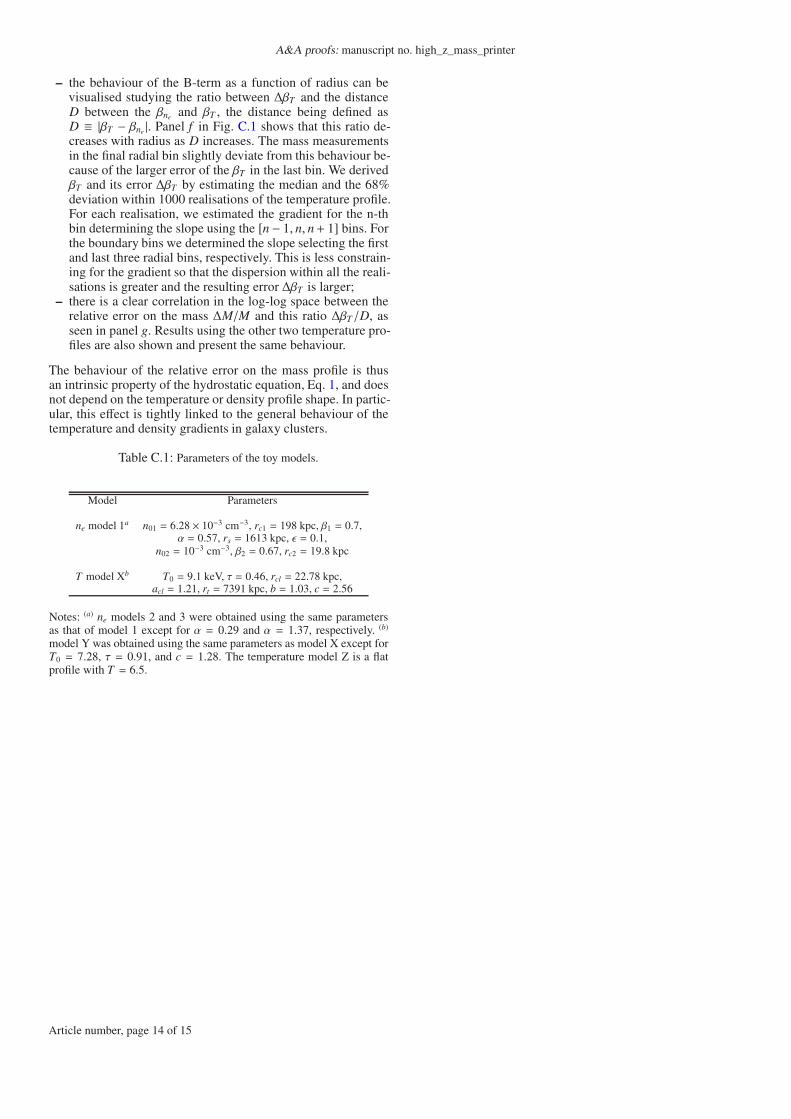
Table C.1: Parameters of the toy models.

Model Parameters

ne model 1a n01 = 6.28 × 10−3 cm−3, rc1 = 198 kpc, β1 = 0.7,α = 0.57, rs = 1613 kpc, ǫ = 0.1,

n02 = 10−3 cm−3, β2 = 0.67, rc2 = 19.8 kpc

T model Xb T0 = 9.1 keV, τ = 0.46, rcl = 22.78 kpc,acl = 1.21, rt = 7391 kpc, b = 1.03, c = 2.56

Notes: (a) ne models 2 and 3 were obtained using the same parametersas that of model 1 except for α = 0.29 and α = 1.37, respectively. (b)

model Y was obtained using the same parameters as model X except forT0 = 7.28, τ = 0.91, and c = 1.28. The temperature model Z is a flatprofile with T = 6.5.



Fig. C.1: For all the panels except panel g: points represent the quantity measured at fixed radial bins. The solid line is showed to guide the eye.Panel a: density profiles generated using the parametric model of Vikhlinin et al. (2006). The errors are set to 0. Panel b: temperature profilesgenerated using the parametric model of Vikhlinin et al. (2006). The relative error on each bin is fixed to 6%. For clarity, bins and correspondingerrors are reported only for ‘T model X’. We report only the shape form of ‘T model Y’ and ‘T model Z’ with solid grey and magenta lines,respectively. Panel c: hydrostatic mass profiles derived from the three density profiles and from the temperature profile ‘T model X’ shown inpanel a and b, respectively, using the FP method. Panel d: β is defined as the logarithmic derivative of the density and temperature, namely β(ne)and β(kT ), with respect to the logarithm of the radius, β ≡ ∂ ln x/∂ ln r. The errors of β(kT ) are derived via a Monte-Carlo procedure. Panel e:temperature and mass profile relative errors as a function of the radius. The dotted line represents the 6% relative error. The mass profiles arecomputed using the three density profiles and the ‘T model X’. Panel f: ratio between the error of β(kT ) and the distance D between β(ne) andβ(kT ), the distance being defined as D ≡ |β(kT ) − β(ne). Panel g: mass profile relative errors as a function of the same quantity shown on the yaxis of panel f. For this plot, we also included the results using all the temperature profiles. Points are colour-coded in order to clearly identify theinner core (blue points, upper right part of the plot) and the outskirts (red points, lower left part of the plot).


Resolving the hydrostatic mass proﬁles of galaxy clusters ...

Documents

Transcript of Resolving the hydrostatic mass proﬁles of galaxy clusters ...