Resolution of reservoir scale electrical anisotropy from marine CSEM data

Vanessa Brown1, Mike Hoversten2, Kerry Key3, and Jinsong Chen4

ABSTRACT

A combination of 1D and 3D forward and inverse solutions isused to quantify the sensitivity and resolution of conventionalcontrolled source electromagnetic (CSEM) data collected usinga horizontal electric dipole source to transverse electric aniso-tropy located in a deep-water exploration reservoir target. Be-cause strongly anisotropic shale layers have a vertical resistivitythat can be comparable to many reservoirs, we examined howCSEM can discriminate confounding shale layers through theircharacteristically lower horizontal resistivity. Forward modelingindicated that the sensitivity to reservoir level anisotropy is verylow compared with the sensitivity to isotropic reservoirs, espe-cially when the reservoir is deeper than about 2 km below the

seabed. However, for 1D models where the number of inversionparameters can be fixed to be only a few layers, both vertical andhorizontal resistivity of the reservoir can be well resolved usinga stochastic inversion. We found that the resolution of horizontalresistivity increases as the horizontal resistivity decreases. Thiseffect is explained by the presence of strong horizontal currentdensity in anisotropic layers with low horizontal resistivity.Conversely, when the reservoir has a vertical to horizontal re-sistivity ratio of about 10 or less, the current density is verticallypolarized and hence has little sensitivity to the horizontal resis-tivity. Resistivity anisotropy estimates from 3D inversion for 3Dtargets suggest that resolution of reservoir level anisotropy for3D targets will require good a priori knowledge of the back-ground sediment conductivity and structural boundaries.

INTRODUCTION

The field of marine controlled source electromagnetics (CSEM)has made major advances in most aspects of data-acquisition andinterpretation over the last ten years. A significant step in interpre-tation capability came with the recognition of the importance ofelectrical anisotropy in the measured CSEM responses. The effectof electric anisotropy has been the subject of many papers: in deepcrustal studies (Everett and Constable, 1999), fracture detection andmapping (Le Masne and Vasseur, 1981), mineral exploration(Al-Garni and Everett, 2003), and in borehole logging (Lu andAlumbaugh, 2001). Barber et al. (2004) demonstrate how electricanisotropy can be determined through borehole logging. Ellis et al.(2010) developed an effective medium model for sediment aniso-tropy arising through preferred grain shape and alignment.Initial recognition of the importance of electric anisotropy for

marine CSEM has focused on the relatively modest macroscale

anisotropy where the ratio of vertical (Rvert) to horizontal (Rhorz)resistivity ranges between one and three. The effect of this macro-scale electric anisotropy in hydrocarbon exploration has beenshown to be significant (e.g., Tompkins, 2004, 2005; Hoverstenet al. 2006; Lu and Xia 2007). The overburden anisotropy has beenshown to produce larger effects than anisotropy at the reservoir level(e.g., Tompkins, 2005, Li and Dai, 2011). Newman et al. (2010)show that accounting for electric anisotropy in the backgroundmodel was essential in fitting offline, or the so-called broadside,CSEM data. More importantly, the ability to fit the broadside dataimproved the inverted resistivity structure overall.The ability to determine both the vertical and horizontal resistiv-

ity of reservoir sized zones has several applications. In the case ofhydrocarbon-saturated sands with homogeneous grain size, wherethe electric resistivity is expected to be more isotropic, the ability toaccurately image electric anisotropy could help in distinguishing oilsand from anisotropic shale. Shale is the most common rock where

Manuscript received by the Editor 4 May 2011; revised manuscript received 8 November 2011; published online 2 March 2012.1Institut de Physique du Globe de Paris, Paris, France and University of California San Diego, Scripps Institution of Oceanography, La Jolla, California, USA.

E-mail: brown@ipgp.fr.2Chevron Energy Technology Company, San Ramon, California, USA. E-mail: hovg@chevron.com.3University of California San Diego, Scripps Institution of Oceanography, La Jolla, California, USA. E-mail: kkey@ucsd.edu.4Lawrence Berkeley Lab, Earth Sciences Division, Berkeley, California, USA. E-mail: jchen@lbl.com.

© 2012 Society of Exploration Geophysicists. All rights reserved.

E147

GEOPHYSICS, VOL. 77, NO. 2 (MARCH-APRIL 2012); P. E147–E158, 16 FIGS., 2 TABLES.10.1190/GEO2011-0159.1

anisotropy (both acoustic and electric) is generated at themicroscale (although layered shale-sand could have macroscaleanisotropy). Hoversten et al. (2006) present a case where a highlyanisotropic shale layer (Rvert∕Rhorz ∼ 40) had been mistaken for ahydrocarbon bearing sand. In comparison, the vertical resistivity ofmany hydrocarbon-saturated sands can be on the order of 30 Ωm,and in some cases, lower. The latter case places them in the samerange as anisotropic shale. Accurate determination of horizontal re-sistivity could help discriminate between a uniform porosity anduniform grain size sands and highly anisotropic shale.A second application is for the large electric anisotropy that has

also been observed in clean sands with uniform porosity. Andersonet al. (1994) describe anisotropies on the order of 10∶1 and greaterin such sands where the anisotropy is thought to be caused by var-iations in grain size, and hence, permeability (Klein, 1996). Sandswith uniform porosity but variable permeability and grain size areelectrically isotropic when filled with pore water, only becominganisotropic with the introduction of hydrocarbons. This leads tothe intriguing possibility of making permeability estimates in hy-drocarbon filled sands from inferred electric anisotropy if suchan inference were possible. This also means that the transition fromregions of isotropic resistivity to regions of anisotropic resistivitywould mark the transition from water to oil within reservoir sands,as demonstrated by Klein et al. (1997). A third related application isthe use of the horizontal and vertical resistivity as independent datain stochastic rock physics simulations of fluid type, where the abil-ity to accurately determine horizontal resistivity is essential.The electromagnetic field originating from a horizontal electric

dipole (HED) source can be decomposed into two modes, trans-verse electric (TE) and transverse magnetic (TM), where transverserefers to the field orthogonal to some symmetry axis. For 1D mod-els, the symmetry is about the vertical axes. The TE mode is char-acterized by horizontal electric current loops, where couplingbetween layers is purely inductive; the TM mode is characterizedby vertical electric current loops (and horizontal magnetic fieldloops), where coupling between layers is both galvanic and induc-tive. When the source and receivers are inline (i.e., the source dipoleis pointing along the receiver line) a thin resistive reservoir can bedetected by an anomalous electromagnetic field at source receiveroffsets typically about 3–6 times the target depth (e.g., Orange et al.,2009). If the electric field is recorded by receivers in the purelybroadside (offline) configuration (i.e., the source to receiver linemakes a 90 degree angle with the dipole), the anomalous electricfield due to the resistive target layer is significantly lower thanthe inline case (e.g., Constable and Weiss, 2006). Inspection ofthe field line shape from a HED source shows there are morevertical electric field lines per unit area through the buried resistordirectly below and inline with the source compared with offline.The electric fields measured inline will be dominated by the TMmode with a much smaller TE component. The resistive layer actsas an efficient barrier shielding deeper conductors from the TMmode vertical current loops and generates the detectable anomalousresponse. Conversely, beneath the broadside receivers there aremore horizontal field lines through the buried resistor, thereforethe TE mode will contribute more to the broadside and offline data.Despite the high resistivity of a reservoir, its thinness precludes sig-nificant inductive attenuation; hence the horizontally polarized TEenergy is relatively unmodified by its presence. Consequently, it isgenerally considered that TM mode and galvanic effects are key in

generating the anomalous field and hence allowing for the detectionof the resistor (e.g., Weidelt, 2007). In contrast to the TE and TMmodes produced by a HED source, a vertical electric dipole source(VED) will produce only a TM mode, and therefore, offers lowerresolution of target layers (e.g., Key 2009). For higher dimensionalfeatures, the TE mode description may no longer be valid in thevicinity of the anomalous structure due to galvanic effects generatedalong its lateral edges.If anisotropy is present the electromagnetic fields detected can be

further modified. Ramananjaona (2010) demonstrates that the TMmode is sensitive to the vertical resistivity and the anisotropic ratio,whereas the TE mode is more sensitive to the horizontal resistivity.By examining the reflection coefficients, Ramananjaona (2010)shows that an anisotropic layer of resistivity (Rhorz, Rvert) and thick-ness H, has an equivalent isotropic layer for each mode. For the TEmode, the equivalent isotropic layer is thickness H 0 ! H and resis-tivity R 0 ! Rhorz, whereas for the TM mode the equivalent layer hasresistivity R 0 ! Rvert and thickness H 0 ! !H. The ! term, which isthe anisotropy ratio (

pRvert∕Rhorz), leads to this noncomplete

equivalence between the isotropic and the anisotropic model, sup-porting the argument that isotropic modeling can be insufficient forvery anisotropic structures.Overall, HED sources, which generate both TM and TE modes,

appear to be more sensitive to vertical resistivity (whether in theoverburden, basement, or in the reservoir) than horizontal resistiv-ity. Sensitivity to horizontal resistivity, to whatever extent it exists,arises from horizontal current flow from either the inductive com-ponent associated with TE mode propagation or from the horizontalpart of the TM field. To our knowledge, Abubakar et al. (2010) pre-sent the only work to date that has specifically addressed the abilityto resolve electric anisotropy of the reservoir. This work was doneusing 2D models and only considered data that is inline with eitherelectric or magnetic transmitters. They concluded that both horizon-tal magnetic dipole sources with horizontal magnetic field receiversand horizontal electric dipole sources with horizontal electric fieldreceivers are required to adequately discriminate both horizontaland vertical resistivity. However, their work did not consider thesensitivity of offline data from horizontal electric dipole sources.While the benefits of a magnetic dipole source for determiningthe horizontal reservoir resistivity are suggested by Abubakaret al. (2010), there is currently no commercial system available withsuch a source. We therefore have chosen to study the ability, or lackthereof, to determine vertical and horizontal resistivity in reservoirsusing only commercially available inline and offline data configura-tions (i.e., that obtained from horizontal electric dipole sources)We begin with 1D modeling studies demonstrating the magnitude

and location of sensitivity to anisotropy in a deep target example.We also include the same type of study for a 3D slab model exam-ple. We then use stochastic 1D inversion simulations and 2D finiteelement modeling to characterize how well various reservoir aniso-tropies can be resolved. We finish this work with 3D deterministicinversions of anisotropic versus isotropic deep targets to furthercharacterize how well anisotropy may be resolved in a more realisticdata set.

1D SENSITIVITY STUDY

In this section, we use layered 1D models to investigate thesensitivity of simulated HED CSEM data to horizontal anisotropylocated only in a target reservoir layer. The models, shown in

E148 Brown et al.

Figure 1 and described in Table 1, contain an anisotropic 100-m-thick target layer at depths of 1, 2, and 3 km below the mud line(BML) in an isotropic host (models 1, 2, and 3, respectively). Forcomparison, data are also simulated for a 3D reservoir slab modelidentical to model 2 except the target is a 5 by 5 km slab at 2 kmBML. In the target layer Rvert is fixed at 40 !m and Rhorz is variedfrom 1 to 40!m to allow a range of anisotropies, with the end mem-bers representing a homogeneous shale and a homogeneous oilfilled sand, respectively. The simulated data-acquisition geometryis a single receiver located at the origin. The source is an x-directedhorizontal electric dipole (HED) traversing on 17 east–west saillines with an x range from −15 to"15 km. The sail lines are spaced1 km apart in the y-direction with the sail line array centered on thereceiver location. Source points on each sail line are spaced 250 mapart. Five frequencies (0.125, 0.25, 0.5, 1, 2 Hz) representative ofcommon field acquisition are simulated. Received electric fieldsthat are parallel to the source dipole (Ex) are referred to as max-coupled, whereas electric fields orthogonal to the source dipoles(Ey) are referred to as null-coupled.Figure 2 shows the Ex and Ey field amplitude for model 2 with no

target layer, with an isotropic target layer (Riso ! 40 Ωm) and withan anisotropic target layer (Rvert ! 40 Ωm and Rhorz ! 1 Ωm).Data at 0.5 Hz is shown because it is the frequency of maximumresponses for this model. Figure 2 shows the difference between thetarget-layer and the no-target-layer case is clear for the Ex ampli-

tudes and more difficult to see for the Ey amplitudes. The differencebetween the data from models with an anisotropic and with an iso-tropic target layer is very small in Ex and Ey, and the details cannotbe readily discerned. These differences in the electric field betweenthese two target types are typically on the same order of magnitudeas the noise level.In this first section of the paper we have chosen to examine the

difference between responses from an isotropic target and ananisotropic model relative to the expected data noise level to moreaccurately access the level of sensitivity to the anisotropy. We havechosen the expression in equation 1 as sensitivity sE:

sE ! jEaniso − EisojjEnoisej

; (1)

which is relative to the noise level. The sensitivity to the horizontalanisotropy is defined as the difference between field amplitudes (weuse Ex or Ey) from a model with an anisotropic resistive layer Eaniso,and the field amplitude from a model with an isotropic resistivelayer model Eiso, divided by a model of the expected noise measure-ment to quantify the sensitivity potentially obtainable in a commer-cial data set. A sensitivity sE value of two implies the differencebetween the anisotropic and isotropic electric field values is twicethe noise value, Enoise, at that location. We define the noise as

Enoise !!!!!!!!!!!!!!!!!!!!!!!!!!!!!!!!!!!E2rel " E2

rot " E2abs

q. (2)

There are three contributions to the noise. The first contribution is arelative error (Erel) in the field amplitude expressed as a percentageof the amplitude. This can be due to systematic measurement orinstrumental error and is assigned to be 5% in this study. The

Table 1. Table of synthetic models used for forwardmodeling.

Target DepthBML

AnisotropicRvert∶Rhorz

IsotropicRvert∶Rhorz

Model 1 1 km 40∶1 40∶40Model 2 2 km 40∶1, 40∶2.5, 40∶5,

40∶10, 40∶2040∶40

Model 3 3 km 40∶1 40∶403D Slab 2 km 40∶1 40∶40

10!18

10!16

10!14

10–12

Ex

Ey

AnisotropicIsotropicNo Target

A

mpl

itude

(V

/Am

2 )

10!18

10!16

10!14

10–12

A

mpl

itude

(V

/Am

2 )

Noise floor

Distance along towline (km)

–15 –10 –5 0 5 10 15

–15 –10 –5 0 5 10 15

a)

b)

Figure 2. Field amplitudes Ex and Ey at 0.5 Hz for model 2. The Exdata is inline (a); the Ey data is 3 km offline (b); three variations ofmodel 2 shown: with no target layer, an isotropic target layer and ananisotropic target layer.

Sea Layer 0.3 m

2 m

4 m

2.5 km

0 km

1,2,3 km

0.1 km

Layer: R ,R horz vert

Sea Layer 0.3 m

2 m

2.5 km

0 km

2 km

4 m

5 km Slab: R ,R horz vert

0.1 km

3D Slab ModelModel 1, 2, 3a) b)

Figure 1. (a) Models 1, 2, 3 are shown. (b) Three-dimensional slabmodel consists of a 100 m thick, 5 by 5 km slab. Resistivity valuesare given in Table 1.

Reservoir anisotropy from CSEM data E149

absolute error (Eabs) is the transmitter-receiver system noise floor,which we take to be an optimistic 10−16 V∕Am2 in this study. Theerror due to rotation (Erot) specifically arises from the uncertainty inthe receiver dipole orientation. If " is a small error in the rotationangle, Fx and Fy are the fields we measure, then the true fields Ex,Ey, can be given by the following matrix equation:

"ExEy

#!

"cos # sin #− sin # cos #

#"FxFy

#: (3)

The error due to this rotation error is then ΔEx ! Ex − Fx. Withsome manipulation it can be shown that

jΔExrot j !!!!!!!!!!!!!!!!!!!!!!!!!!!!!!!!!!!!!!!!!!!!!!!!!!!!!!!!!!!!!!#cos # − 1$2jExj2 " sin2 #jEyj2

q; (4)

jΔEyrot j !!!!!!!!!!!!!!!!!!!!!!!!!!!!!!!!!!!!!!!!!!!!!!!!!!!!!!!!!!!!!!#cos # − 1$2jEyj2 " sin2 #jExj2

q: (5)

The total error is then given by

jExnoise j !!!!!!!!!!!!!!!!!!!!!!!!!!!!!!!!!!!!!!!!!!!!!!!!!!!!!!!!!!!!!!!!!!!!!!!!!!!!!!!!!!!!!!!!!!!!!!!!$2jExj2 " #cos # − 1$2jExj2 " sin2 #jEyj2 " E2

abs

q;

(6)

jEynoise j !!!!!!!!!!!!!!!!!!!!!!!!!!!!!!!!!!!!!!!!!!!!!!!!!!!!!!!!!!!!!!!!!!!!!!!!!!!!!!!!!!!!!!!!!!!!!!!!$2jEyj2 " #cos # − 1$2jEyj2 " sin2 #jExj2 " E2

abs

q:

(7)

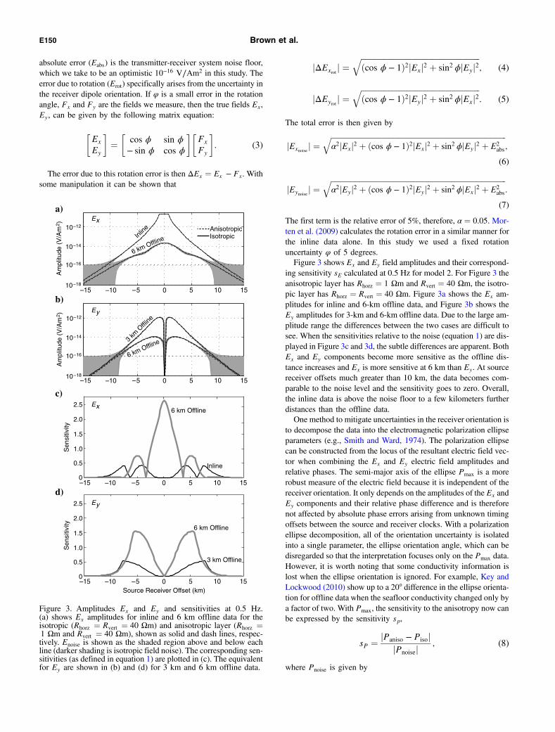
The first term is the relative error of 5%, therefore, $ ! 0.05. Mor-ten et al. (2009) calculates the rotation error in a similar manner forthe inline data alone. In this study we used a fixed rotationuncertainty " of 5 degrees.Figure 3 shows Ex and Ey field amplitudes and their correspond-

ing sensitivity sE calculated at 0.5 Hz for model 2. For Figure 3 theanisotropic layer has Rhorz ! 1 Ωm and Rvert ! 40 Ωm, the isotro-pic layer has Rhorz ! Rvert ! 40 Ωm. Figure 3a shows the Ex am-plitudes for inline and 6-km offline data, and Figure 3b shows theEy amplitudes for 3-km and 6-km offline data. Due to the large am-plitude range the differences between the two cases are difficult tosee. When the sensitivities relative to the noise (equation 1) are dis-played in Figure 3c and 3d, the subtle differences are apparent. BothEx and Ey components become more sensitive as the offline dis-tance increases and Ex is more sensitive at 6 km than Ey. At sourcereceiver offsets much greater than 10 km, the data becomes com-parable to the noise level and the sensitivity goes to zero. Overall,the inline data is above the noise floor to a few kilometers furtherdistances than the offline data.One method to mitigate uncertainties in the receiver orientation is

to decompose the data into the electromagnetic polarization ellipseparameters (e.g., Smith and Ward, 1974). The polarization ellipsecan be constructed from the locus of the resultant electric field vec-tor when combining the Ex and Ey electric field amplitudes andrelative phases. The semi-major axis of the ellipse Pmax is a morerobust measure of the electric field because it is independent of thereceiver orientation. It only depends on the amplitudes of the Ex andEy components and their relative phase difference and is thereforenot affected by absolute phase errors arising from unknown timingoffsets between the source and receiver clocks. With a polarizationellipse decomposition, all of the orientation uncertainty is isolatedinto a single parameter, the ellipse orientation angle, which can bedisregarded so that the interpretation focuses only on the Pmax data.However, it is worth noting that some conductivity information islost when the ellipse orientation is ignored. For example, Key andLockwood (2010) show up to a 20° difference in the ellipse orienta-tion for offline data when the seafloor conductivity changed only bya factor of two. With Pmax, the sensitivity to the anisotropy now canbe expressed by the sensitivity sp,

sP ! jPaniso − PisojjPnoisej

; (8)

where Pnoise is given by

AnisotropicIsotropicInl

ine

6 km Offline

3 km O

ffline

6 km Offline

Ex

Ey

Ex

Ey

Source Receiver Offset (km)

0

1.0

0.5

1.5

2.0

2.5

0

1.0

0.5

1.5

2.0

2.5

–15 –10 –5 0 5 10 15

–15 –10 –5 0 5 10 15

–15 –10 –5 0 5 10 15

–15 –10 –5 0 5 10 15

6 km Offline

6 km Offline

Inline

3 km Offline

Sen

sitiv

ityS

ensi

tivity

10–12

10!14

10!16

10!18

Am

plitu

de (

V/A

m2 )

10–12

10!14

10!16

10!18

Am

plitu

de (

V/A

m2 )

a)

b)

c)

d)

Figure 3. Amplitudes Ex and Ey and sensitivities at 0.5 Hz.(a) shows Ex amplitudes for inline and 6 km offline data for theisotropic (Rhorz ! Rvert ! 40 Ωm) and anisotropic layer (Rhorz !1 Ωm and Rvert ! 40 Ωm), shown as solid and dash lines, respec-tively. Enoise is shown as the shaded region above and below eachline (darker shading is isotropic field noise). The corresponding sen-sitivities (as defined in equation 1) are plotted in (c). The equivalentfor Ey are shown in (b) and (d) for 3 km and 6 km offline data.

E150 Brown et al.

Pnoise !!!!!!!!!!!!!!!!!!!!!!P2rel " P2

abs

q; (9)

where Prel is an assumed 5% noise of the Pmax values for theanisotropic layer fields, and is due to systematic instrumental mea-surement errors; Pabs is an absolute error floor taken to be10−16 V∕Am2. Notice in this case there is no rotation error becausewe utilize both x- and y-components in the polarization calculation.A sensitivity sp value of two implies the difference between theanisotropic and isotropic Pmax values is twice the typical error valuePnoise, at that location.To visualize the location of highest sensitivity, Figure 4 displays

the values sE and sp calculated for the entire survey area for models1, 2, and 3. The plots also contain gray contour lines that mark the10−15 V∕Am2 (inner) and the 10−16 V∕Am2 (outer) amplitudelevels, where the 10−16 V∕Am2 contour is the noise floor usedin sensitivity formulations shown earlier (Eabs). The data locatedoutside this contour are below the noise floor and hence wouldnot be obtainable in a real survey. The rapid diminishing of sensi-tivity as the source receiver distance increases is due to the datareaching this noise floor. The white contour is where the sensitivity,sE or sp, is equal to one and is where the difference between theanisotropic and isotropic fields or polarization parameters is equalto the noise level. The colored regions contained within the whitecontours are where the responses have sensitivity above the noisefloor, and thus, where it is possible to discriminate the subtle ani-sotropic signal.The first column in Figure 4 shows the sensitivity using the Ex

field amplitude. At very short offsets the anisotropic sensitivity iszero due to the basic lack of sensitivity to the deep reservoir. Thesensitivity increases moving away from the source in general due tothe increased coupling with the reservoir, but there is a marked geo-metry aspect to the Ex sensitivity. The purely inline and offline(broadside) regions have the highest sensitivity, but this diminishesrapidly where the Ex amplitude drops to zero due to the basic dipolegeometry (roughly along 45 degree azimuths). The maximum sen-sitivity value for models 1, 2, and 3 are found atoffline distances of 7, 6, and 6 km, respectivelyalong x ! 0 km, directly perpendicular to thex-pointing dipole source. For models 1 and 2,the peak sensitivity value is around seven andfour, respectively. For model 3 where the targetis at 3 km BML, the sensitivity barely exceedsone for any source location.The second column in Figure 4 shows the sen-

sitivity to the Ey field amplitude component. Inthis case, the regions with sensitivity above one(above the noise level) all reside offline inpatches away from the x- and y-axes, as ex-pected, given that Ey component has zero ampli-tude along the x- and y-axes due to the dipolegeometry. The sensitivity tends to increase mov-ing further offline away from the source axis. Formodel 1 where the target is at 1 km depth, theregion of high sensitivity covers a greater spatialextent for Ey data compared with the Ex data;however, the peak values are lower. Overall,the Ey component sensitivities are lower thanEx and do not exceed a value of three, evenfor the shallowest target.

The Pmax sensitivities for models 1, 2, and 3 are shown in thefinal column. Because Pmax is computed using both Ex and Ey,its sensitivity has a shape that is a combination of the sensitive re-gions of the individual components. The highest sensitivity to theanisotropy is consistently in the furthest offline data within the noisefloor boundaries. To a lesser extent, there is sensitivity in the inlineregions that are lower and lie further from the source compared withthe offline data, giving the sensitivity an ellipsoidal shape that iselongated in the inline (x) direction. Model 1 has a peak sensitivityof around 7.5, model 2 the peak is around four. Model 3 does nothave sensitivity above the noise floor, despite Pmax being insensitiveto the rotation error.Figure 5 shows the peak sensitivities sE over the entire survey

area as a function of source frequency and a range of target layeranisotropy values created by increasing the Rhorz in the layer from 1to 20 !m (Rvert ! 40 Ωm). This study was done for model 2 wherethe target layer is 2 km BML. The largest sensitivity above the noisefloor is in the range of 0.25–1 Hz with a peak at 0.5 Hz. The sen-sitivity rapidly decreases for both higher and lower frequencies. AsRhorz increases and the layer becomes less anisotropic, the sensitiv-ity to anisotropy decreases, as expected (by definition it goes to zerofor a perfect isotropic layer). Figure 5 shows that at 0.5 Hz the Exsensitivity becomes very small even for a modest increase in Rhorz

from 1 to 5 !m, which corresponds to a ratio (Rvert∶Rhorz)40∶1 to 40∶5. The Ex sensitivity changes from greater than fourto less than one at 0.5 Hz. When Rhorz is 5 !m (ratio 40∶5), itis comparable to the background value of Rhorz (4 !m) and the dif-ference between the isotropic and anisotropic fields would be dif-ficult to detect without further stacking of the data, or without futureinstrumental improvements to lower the source-receive noise floor.The Ey sensitivities show a similar pattern, but overall, have muchlower sensitivity than Ex.Figure 6 shows the sensitivity for the 3D slab described in Table 1

using the same sensitivity definition and color scales as in Figure 4.Note that in this study the depth of the target is held fixed at 2 km

Sensitivity of Ex

1ledoM

2ledoM

3ledoM

Sensitivity of Ey Sensitivity of Pmax

)mk(

noitisoP

y

1 2 3 4 5 6 7 8

!10 !5 0 5 10x Position (km)x Position (km)

!10 !5 0 5 10x Position (km)

!10 !5 0 5 10

8

4

0

8

4

0

–8

–4

–8

–4

–8

–4

8

4

0

Sensitivity

)mk(

noitisoP

y)

mk(noitiso

Py

Figure 4. Sensitivity to the anisotropy is shown for Ex, Ey components and for Pmax formodels 1, 2, and 3. The white contour marks where these sensitivities are equal to oneand the gray contours mark the 10−15 V∕Am2 (inner) and the 10−16 V∕Am2 (outer)noise floor. Red arrows show the HED position.

Reservoir anisotropy from CSEM data E151

depth, and the three rows represent scenarios where the source isplaced at the origin, at 4 and 6 km from the origin along the y-axis.Overall the sensitivities are significantly less than for the layeredmodel at the same depth of 2 km (second row in Figure 4). TheEy component alone is now insensitive to the anisotropy, suggestingthat the Ey sensitivity in the 1D studies depends on the large lateralextent of the target. When the source is directly over the target(shown in the top row), the sensitivity is above the noise level onlyfor the offline Ex responses. The middle row shows the target iscoupled optimally when the source is located 4 km from the targetcenter, as illustrated by the peak sensitivity of around three. Thesensitive data are localized to a small region located 6–8 km offline.The bottom row shows the data collected when the source is at 6 kmfrom the origin, again there is sensitivity offline but it is lower than

the optimally coupled 4-km source position. The Pmax sensitivitiesfor each case tend to reflect the Ex sensitivities because the Ex com-ponent is the main contributor.

STOCHASTIC INVERSIONS

In this section we use the 1D stochastic inversion algorithm de-veloped by Chen et al. (2007) to determine the ability to resolve theanisotropic parameters of a resistive target in model 2 in an inversesense. We assume that the location and thickness of the reservoirtarget can be determined from seismic data or other information.We estimate Rvert and anisotropy ratio !. The resistivity of seawater,the overburden, and the bedrock are also considered unknowns. Weestimate parameters using data along two survey lines, inline (y !0 m) and offline (y ! 6 km), for a model with an isotropic target(Rhorz ! Rvert ! 40 Ωm) and an anisotropic target (Rhorz ! 1 Ωmand Rvert ! 40 Ωm). We use the same priors for the two cases andassume that Rvert is uniformly distributed on (1, 200) !m, and theratio Rvert∕Rhorz is uniformly distributed on (1, 100). The priordistributions of seawater, overburden, and bedrock resistivity areuniformly distributed on (0.1, 1.0) !m, (1, 10) !m, and(1, 10) !m, respectively. Although this 1D example is a simplifiedmodel with a very small number of parameters (five) and is not re-presentative of the resolution that could be achieved in real-worldinversions of field data without perfect a priori knowledge of thelayer boundaries, it merely serves to illustrate the relative differ-ences in resolution of Rhorz versus Rvert for different data types(i.e., inline and offline data).Markov chain Monte Carlo methods are used to explore the joint

posterior distribution of unknowns. A hybrid sampling strategydescribed in Chen et al. (2007) is used. The sampling methodsinclude (1) single variable Metropolis-Hastings methods (SMH)(Metropolis et al., 1953; Hastings et al., 1970), (2) multivariateMetropolis-Hastings methods (MMH), (3) single variable slice sam-pling methods (SSS) (Neal, 2003), and (4) multivariate slice sam-

pling methods (MSS). At each iteration, werandomly select one of the above methods for up-dating. We start from five different sets of initialvalues, which are the lower bounds, upperbounds, median, 25% quantile, and 75% quan-tiles of the prior bounds. We use the potentialscale reduction factor (PSRF) to monitor the con-vergence of the five chains using the method byBrooks and Gelman (1998), which is a measureof the between-chain variability relative to thewithin-chain variability. With that approach, ifthe scale reduction score is less than 1.2, the Mar-kov chain is considered converged; otherwise,more runs are needed.The stochastic inversion was run with 5%

Gaussian noise added to the synthetic data.Figure 7a and 7b shows the parameter probabilitydensity functions (PDFs) obtained for the hori-zontal and vertical resistivity for the isotropictarget model. Based on the forward modeling re-sults, we would expect the inline data to have thehighest sensitivity to Rvert and the offline data tohave the highest sensitivity to Rhorz, which isconsistent with the mode and standard deviationsof these parameters listed in Table 2. The mode

0.5 1.0 1.5 2.00

1.0

2.0

3.0

4.0

Frequency (Hz)

Max

imum

Sen

sitiv

ity

0.5 1.0 1.5 2.0Frequency (Hz)

1 !m 2.5 !m

5 !m 10 !m 20 !m

EyEx

Rhorz

a) b)

Figure 5. The peak sensitivity extracted from the contour plots formodel 2 is plotted against frequency. The values are plotted for arange of anisotropy ratios indicated by the variation of Rhorz fromone to 20 !m, whereas Rvert is fixed at 40 !m. Figure (a) shows theEx component data and (b) Ey.

!10 !5 0 5 10x Position (km)

y P

ositi

on (

km)

y P

ositi

on (

km)

y P

ositi

on (

km)

!10 !5 0 5 10x Position (km)

!10 !5 0 5 10x Position (km)

Sensitivity of Ex Sensitivity of Ey Sensitivity of Pmax 8

4

0

8

4

0

–4

–8

–4

–8

–4

–8

8

4

0

1 2 3 4 5 6 7 8

Sensitivity

Figure 6. Sensitivity to the anisotropy for Ex, Ey components and for Pmax for the 3Dslab model. The white contours marks where these sensitivities are equal to one and thegray contours mark the 10−15 V∕Am2 and the 10−16 V∕Am2 noise floors of the data.Red arrows show the source dipole position.

E152 Brown et al.

of both the inline and offline PDFs are within 1% of Rvert, as ex-pected. Conversely, for Rhorz, the offline mode is within 15%,whereas the mode of the inline data is 38% too low. This resultindicates that there is information about Rhorz in the inline becausethe PDF clearly indicates it is resistive. The larger parameter stan-dard deviations (width of the PDFs) for Rhorz compared with Rvert

reflects the lower sensitivity to Rhorz, which was seen in the forwardmodeling studies.The parameter PDFs for the anisotropic target layer are shown in

Figure 8a and 8b. The results for Rvert are consistent with that of theisotropic case, with the PDFs for both inline and offline data within1% of the true values. The PDFs for Rhorz show that both the inlineand offline data resolve the Rhorz better than the isotropic case. Themode is closer to the true value and the standard deviation smallerusing the offline data compared with the inline.The stochastic inversions lead to two main conclusions; first, that

Rvert of the 1D target layer is well resolved by both inline and offlinedata, and second, that the anisotropic layer Rhorz of 1 !m is muchbetter resolved than the more resistive isotropic layer Rhorz of 40 !m. To further explore how the ability to resolve Rhorz may be af-fected by the value of Rhorz in the target layer, data were simulatedfor anisotropic models and a reference model with the same geo-metry as model 2. In this section the reference model target layerRhorz is equal to the basement Rhorz of 4 !m and Rvert is 40 !m. Theanisotropy is varied in the target layer by fixing Rvert at 40 !m andvarying Rhorz 1–20 !m, which ranges from less than to greater thanRhorz of the reference model. For each model, a percentage differ-

ence is calculated to determine how sensitive the electric field re-sponse is to the value of Rhorz compared with the background value.Here we are concerned with the variation in field response as Rhorz isvaried and we are unconcerned with the measurement noise. Theequation

sPD ! jEaniso − Eref jjEref j

! 100; (10)

where Eaniso is the Ex field for the anisotropic reservoir and Eref isthe Ex field from the reference model is used. This percentage dif-ference, sPD, versus the target layer Rhorz is plotted in Figure 9a and9b for inline and 6 km offline data, respectively. For the inline andoffline cases there is a large increase in percentage difference asRhorz becomes more conductive than the reference/background va-lue. There is a much smaller increase as Rhorz becomes more resis-tive than the background. In both cases, all data below the noisefloor are removed which explains why the offline figure (Figure 9b),despite being more sensitive to the anisotropy, only contains the twolowest frequencies. The large gradient as Rhorz is made more con-ductive compared with more resistive explains why the stochasticinversion resolves the conductive Rhorz better than the resistiveRhorz. When Rhorz is more resistive than 4 !m (the background),the change in electric field response decreases. This effect appearssimilar to the saturation effect observed for the magnetotelluricmethod, where the magnetotelluric response can be shown to satu-rate once the resistivity contrast for a resistive layer reaches a certain

0 100 200 300 400 5000

0.005

0.01

0.015

Resistivity (ohm!m)

Pro

babi

lity

Den

sity

Isotropic Rhorz

InlineOfflineTrue value

39.5 40 40.5 41 41.5 420

0.5

1

1.5

2

2.5

3

3.5

Resistivity (ohm!m)

Pro

babi

lity

Den

sity

Isotropic Rvert

InlineOfflineTrue value

a) b)

Figure 7. Probability density functions obtained from stochastic in-version for the isotropic target layer. (a) Inline (black) and offline(red) PDFs for Rhorz. (b) Inline (black) and offline (red) PDFs forRvert. True values shown as a blue line.

Table 2. Table of mode and standard deviations for target layer parameters in model 2 from stochastic inversions with 5% noiselevel.

Isotropic target Anisotropic target

Inline Offline Inline OfflineRvert Rhorz Rvert Rhorz Rvert Rhorz Rvert Rhorz

Value 40 40 40 40 40 1 40 1Mode 40.12 25.41 40.22 34.35 40.18 1.03 40.17 1.00StD 0.105 67.1 0.170 49.2 0.104 0.055 0.216 0.019

0.8 1 1.2 1.40

5

10

15

20

25

Resistivity (ohm!m)

Pro

babi

lity

Den

sity

Anisotropic Rhorz

InlineOfflineTrue value

39.5 40 40.5 41 41.5 420

0.5

1

1.5

2

2.5

3

3.5

Resistivity (ohm!m)

Pro

babi

lity

Den

sity

Anisotropic Rvert

InlineOfflineTrue value

a) b)

Figure 8. Probability density functions obtained from stochastic in-version for the anisotropic target layer. (a) Inline (black) and offline(red) PDFs for Rhorz. (b) Inline (black) and offline (red) PDFs forRvert. True values shown as a blue line.

Reservoir anisotropy from CSEM data E153

limit (typically about a factor of 10 more resistive than the back-ground).To gain further physical insight into this saturation behavior, here

we look at the field and current density sections in the x-z planethrough the target layer for model 2. Figure 10 shows the E fieldand current density polarization ellipses in the x-z axis (y ! 0, in-line) computed using a 2D adaptive finite element code (Key andOvall, 2011) after minor modifications to handle anisotropy. Thebackground color is the Pmax amplitude for the anisotropic reservoircase; the white polarization ellipses are for the anisotropic reservoir,

the black are the isotropic reservoir. Figure 10a shows the electricfield polarizations. However, it is difficult to see the anisotropicellipses (white) underneath the isotropic data ellipses (black), illus-trating that the electric field polarization is nearly identical for theanisotropic and isotropic target cases. Inside the reservoir layer at4.5 to 4.6 km depth, both anisotropic and isotropic fields are verti-cally polarized, as expected from the electromagnetic version ofSnell’s law considered for the TM mode at the boundary betweena conductor and resistor. In Figure 10b, 10c, and 10d, we show theelectric current density polarizations, computed by multiplying theelectric fields by the anisotropic conductivity. Now we can see thatthe current polarizations have a significantly different shape in thereservoir layer, depending on the horizontal resistivity. The isotro-pic target is predominantly vertically polarized, whereas the aniso-tropic target has a large horizontal component and the ellipses aremore horizontally polarized, especially at short offsets. At fartheroffsets there is still a large horizontal current density componentcompared with the isotropic target but at longer offsets the verticalcurrent density component increases fairly rapidly, making the el-lipses vertically polarized. The difference is most pronounced whenRhorz is 1 !m (Figure 10b). As Rhorz increases, the current densityellipses tend to more closely resemble the isotropic case with ver-tical polarization inside the reservoir. Figure 11 shows the horizon-tal and vertical components of the current density at the center of thetarget layer at 3 km offset from the source (x ! 3 km, z ! 4.55 km)for a range of Rhorz with Rvert fixed at 40 !m. As one would expect,the vertical current density stays constant as Rhorz increases becausethe vertical conductivity remains unchanged. The horizontal currentdensity decreases in proportion to 1∕Rhorz, as expected from Ohm’slaw. When Rhorz is less than 2.5 !m, the horizontal current densityis larger than the vertical density, whereas at greater values of Rhorz

the horizontal current density is far below the vertical density. It is atthis point that the field and current are dominantly vertical. There-fore, we can now explain the saturation effect shown in Figure 9 asarising from the transition from horizontally dominated current inthe reservoir to a vertically dominated current when Rhorz becomesgreater than 2.5 !m. Once the polarization is dominantly vertical,

Figure 10. Depth section (x-z plane) through the reservoir. Polar-ization ellipses are shown for the isotropic reservoir case in blackand the anisotropic reservoir in white. Shaded colors indicate thestrength of the polarization-ellipse maximum (anisotropic case).(a) The electric field polarization-ellipses. (b-d) The current densitypolarization ellipses for increasing anisotropies (the colorbar for(c and d) is the same as (b)).

100 10210!14

10!13

10!12

10–11

Horizontal Resistivity (!m)

Cur

rent

Den

sity

(A

m!2

)

Jhorz

Jvert

101

Figure 11. Horizontal and vertical current density in the reservoir atx ! 3 km is plotted against horizontal resistivity.

0

5

10

Offline 0.25 HzOffline 0.5 Hz

2 4 6 8 10 12 14 16 18 200

5

10

Per

cent

age

Diff

eren

ce % Inline 0.25 Hz

Inline 0.5 HzInline 1 Hz

Rhorz (!m) Rhorz (!m)2 4 6 8 10 12 14 16 18 20

Figure 9. Percentage difference sPD (equation 10) used to show thesensitivity to variation in Rhorz normalized by the reference value ofRhorz. Inline data are shown in (a) and offline data in (b).

E154 Brown et al.

sensitivity to the horizontal conductivity has saturated and the sen-sitivity to anisotropy in a target is low.

3D GRADIENT-BASED ANISOTROPIC INVERSION

We have seen from the first two sections, the sensitivity analysisand the stochastic inversions, that there is information in the inlineand offline electric fields that provides high sensitivity to thevertical electric resistivity and to a lesser extent the horizontal elec-tric resistivity of the target layer or slab. In particular, we see thatwhen the horizontal resistivity is conductive relative to the verticaland background resistivity, the 1D stochastic inversion shows it canbe well resolved. However, once the horizontal resistivity becomesresistive relative to the background, it is less well resolved.Unfortunately, most exploration scenarios are not well modeled

by 1D and require at least 2D and often 3D inversion of the fielddata to accurately model potential reservoirs and their surroundingstructures. Although any study of resolution using a specific inver-sion code is always open to the criticism that results are specific tothe code used, we feel it is still instructive. Additionally, we areusing a code that is in wide use throughout the industry, the LBNLEM3D_GEO code (Newman and Alumbaugh, 1997; Newman andHoversten, 2000, Newman et al. 2010).For the 3D inversion studies we use the 3D slab model shown in

Figure 1b, where the target layer is a 5 ! 5 km slab, 100 m thick ata depth of 2 km BML, and with the same vertical and horizontalresistivity used for the 1D model. Frequencies of 0.125, 0.25,0.5, 1.0, and 2.0 Hz are used. The model inversion grid is discre-tized at 150, 150, and 100 m in x, y, and z, respectively. The in-version used a nonlinear transformation of the model parameters tobound resistivity throughout the model to between 0.5 and 100 !m,unless otherwise noted. An array of 25 receivers is laid out symme-trically over the target with 2 km separations in both x and y. Sourcetow-lines of up to 15 km are run over the array with inline and off-line components in both x and y. The maximum offline distance is8 km in the first examples. For the 8 km offsets, we assumed a noisefloor of 10−16 V∕Am2 to allow sufficient number of data at the 8 kmoffsets. A maximum offline distance of 4 km with a 10−15 V∕Am2

noise floor is also considered, reflecting what we normally considerusable data from field operations. The choice of how much offlinedata to use varies with circumstances, some operations use data tolarger offline distances, but we have found that it is generally verynoisy, more so than our simple noise model (% of amplitude plusrotation error) accounts for. We will not speculate on the source ofthis addition error as a function of offline distance but simply note

its existence. Synthetic data was contaminated by Gaussian noisewith standard deviation set to 2% of the amplitude of the electricfield. This value was chosen to match the error level used byAbubakar et al. (2010). All inversions shown are for the iterationwith rms misfit just below 1.0. The inversion started from the truebackground model without the target present. This can be consid-ered a best-case scenario; our experience indicates that the determi-nation of the position and absolute resistivity of targets worsens asthe accuracy of the background (starting) model decreases.We first consider the inversion of the isotropic target where Rhorz

and Rvert is 40 !m. Figure 12 shows vertical cross sections throughthe center of the target body (y ! 0). Figure 13 shows plan views ofthe Rvert and Rhorz at the depth slices of maximum resistivity. We seethe spatial location of the target is well defined (Figure 13a) with themaximum Rvert of 10.5 !m as compared with the true value of 40 !m at a depth 100 m deeper than the target. Rhorz is much less wellresolved. The maximum Rhorz is 2.1 !m at a depth of 3900–4000 mcompared with the true value of 40 !m. While the inverted Rhorz

shows an indication that the target has higher Rhorz than the back-ground it is very slight. In a true 3D environment with variablestructure and background resistivity this variation would not be con-sidered significant. In this case we would not be able to reliablyindicate that the target was either isotropic or anisotropic.The vertical positioning of the anomalous Rvert is enhanced by its

being at the contact between conductive and more resistive materialat 2 km BML. Studies using EM3D_GEO have shown that in a half-space background with no constraints (either removing smoothingacross boundaries, or imposing bounds on allowable resistivity incertain regions) the resistive target would focus approximately 10%(200 m) too shallow. The maximum resistivity will always be lessthan the true value with the difference increasing with depth of thetarget. The lower resistivity is somewhat compensated in the inver-sion with an increase in the thickness so that the reservoir resistiv-ity-thickness product is preserved, as is also typically seen in 1Dinversions (e.g., Key 2009; Brown et al., 2012).Next we consider the anisotropic 3D target where Rvert !

40 Ωm and Rhorz ! 1.0 Ωm. Figure 14 shows the vertical crosssections and Figure 15 the horizontal depth slices. The reconstruc-tion of Rvert in the vertical cross sections is not significantly differ-ent compared with the isotropic case. The maximum resistivity of12.5!m occurs 100 m too deep. The inversion of Rhorz (Figure 14b)has produced a region of lower resistivity, 1.5 !m compared withthe true value of 1.0 !m, which is 200 m too shallow. The spatialimage of both Rvert and Rhorz (Figure 15) shows good agreement

Figure 12. Inversion results for the 3D isotropic target model. Panel (a) shows an x-z cross section of vertical resistivity, and (b) showshorizontal resistivity (x-direction). Location of 3D anisotropic target is shown by black outline, and receiver positions are shown as blacktriangles.

Reservoir anisotropy from CSEM data E155

with the lateral extent of the slab. In this case where the anisotropictarget has more conductive Rhorz, the lateral resolution of Rhorz ismuch better than in the isotropic case (compare Figure 15b withFigure 13b). In these examples, the 3D inversion is insensitiveto anisotropy.Reducing the maximum offline separation from 8 km with a

10−16 V∕Am2 noise floor to 4 km with a 10−15 V∕Am2 noise floorhas only a minor effect on inversion results. The inverted Rvert forthe anisotropic model produces 15 !m as a maximum resistivity,and this occurs at the true depth of 4500–4600 m. This is comparedwith 12.5 !m and 100 m too deep for the 8 km offline inversion ofthe anisotropic model. The isotropic model results are almostidentical.Although a complete study of the effects of inversion constraints

is beyond the scope of this paper, one illustration is worth consider-ing. In practice, prior knowledge including wells, seismic data, and

geology of the basin provide additional constraints that can be usedin inversion. Figure 16 shows the inversion results for the isotropicreservoir model with maximum 4-km offline data and10−15 V∕Am2 noise floor when the upper bound on allowed resis-tivity (Rhorz and Rvert) in the overburden is changed from 100 to10 !m and the inversion’s roughness penalty (i.e., smoothing) isremoved across the top and base of the target slab. Now even withthe reduced amount of data, reflecting a more likely field case, themaximum inverted Rvert reaches 33 !m compared with 12.5 !m inthe less constrained case (Figures 12 and 13). The added constraintshave not, however, improved the resolution of Rhorz.As was seen in the 1D inversion results of the isotropic versus

anisotropic layer, the inversion is more sensitive to conductive Rhorz

than resistive Rhorz. However, the ability to resolve Rvert and Rhorz

for a 3D target is far worse than for a 1D layer. Although one canalways argue that a different algorithm may produce improved

Figure 13. Depth slices through the 3D anisotropic inversion of the isotropic target model. Panel (a) shows vertical resistivity for depth slice4600–4700 m, and (b) shows horizontal resistivity in the x-direction for depth slice 3900–4000 m (location of largest differences from back-ground). Isotropic target is outlined in black, with receiver array shown as black dots.

Figure 14. Inversion results for the 3D anisotropic slab model. Panel (a) shows an x-z cross section of vertical resistivity, and (b) showshorizontal resistivity (x-direction). Location of the 3D anisotropic target is shown by black outline and receiver positions are shown as blacktriangles.

E156 Brown et al.

results, the models found by this algorithm fit the data to better than2% and clearly demonstrate that there is large nonuniqueness in the3D model space. The 3D inversions were also run for the equivalentof model 1, where the slab was moved to 1 km BML. In these tests(not shown), the extreme values of the inverted resistivity camecloser to the true values but still were not nearly as accurate as1D examples with the target layer 1 km BML.

CONCLUSIONS

We conducted a suite of simulation studies to understand the sen-sitivity and resolution capabilities of marine CSEM for detectingelectric anisotropy within a reservoir. Because the horizontal resis-tivity can help distinguish an anisotropic shale from an isotropicreservoir, our studies have paid particular attention to the sensitivityto horizontal resistivity. The 1D sensitivity studies showed that deepwater (2.5 km water depth) CSEM surveys using an HED source are

relatively insensitive to modest anisotropy in a reservoir target. Thisis especially true when the target horizontal resistivity is larger thanthe background horizontal resistivity. By using a somewhat realisticnoise model that includes relative and absolute noise sources, aswell as uncertainty in the receiver orientation, we showed thatthe areas of low but detectable sensitivity are predominantly loca-lized offline at distances of 3–8 km. The sensitivity to the reservoirdiminishes rapidly as the reservoir depth increases and as the ani-sotropy ratio decreases. The sensitivity also decreases rapidly athigher and lower source frequencies than 0.5 Hz. Well-constrainedstochastic 1D inversion results showed that there is sensitivity to thehorizontal resistivity in both inline data, and to a greater extent, inthe offline data. Stochastic inversion results and the deterministic3D inversion results highlight an important consideration in resol-ving transverse anisotropy in a target. That is, as the horizontal re-sistivity decreases below the background resistivity the datasensitivity to the anisotropy increases. If the horizontal resistivity

Figure 15. Depth slices through the inversion results for the 3D anisotropic target model. Panel (a) shows vertical resistivity for depth slice4600–4600 m, and (b) shows horizontal resistivity in the x-direction for depth slice 4300–4400 m (location of largest differences from back-ground). Anisotropic target is outlined in black, with receiver array shown as black dots.

Figure 16. Constrained inversion results for the isotropic 3D slab model. Panel (a) shows an x-z cross section of vertical resistivity, (b) showshorizontal resistivity (x-direction). Location of 3D anisotropic target shown is by black outline and receiver positions are shown as blacktriangles.

Reservoir anisotropy from CSEM data E157

is greater than or comparable to the background resistivity, the dataare far less sensitive to the anisotropy. Although the 3D inversion isunable to resolve the correct horizontal and vertical resistivity, whenthe target horizontal resistivity is more conductive than the back-ground, the resolution is slightly better. In general for the 3D inver-sion (which far is less constrained than the 1D stochastic inversion),the reservoir vertical resistivity is better resolved than the horizontalresistivity, particularly when the horizontal resistivity of the target isgreater than or equal to the background resistivity. Examination ofthe current density polarization within the reservoir shows that thedecreasing sensitivity to horizontal resistivity and hence to aniso-tropy in the reservoir is due to the reservoir current becoming ver-tically dominant as horizontal resistivity increases, resulting in asaturation of the sensitivity to horizontal resistivity.Although the HED source has sensitivity to the target horizontal

resistivity, the sensitivity to the vertical resistivity is greater than thatof the horizontal resistivity. We conclude that to be able to discri-minate modest anisotropy in a deep-water target (2.5 km) usingCSEM either a new source configuration or a combination ofHED and HMD sources may be required.

ACKNOWLEDGMENTS

We are grateful to Chevron Energy Technology Company forsupport and permission to publish this work. Brown and Key ac-knowledge funding support from the Seafloor ElectromagneticMethods Consortium at Scripps Institution of Oceanography. Thiswork was also partially supported by the U.S. Department ofEnergy and LBNL under Contract No. DE-AC02-05CH11231.

REFERENCES

Abubakar, A., 2010, Sensitivity study of multi-sources receivers CSEM datafor TI-anisotropy medium using 2.5D forward and inversion algorithm:Presented at the 72nd Annual Conference and Exhibition, EAGE.

Al-Garni, M., and M. Everett, 2003, The paradox of anisotropy in electro-magnetic loop-loop responses over a uniaxial half-space: Geophysics, 68,892–899, doi: 10.1190/1.1581041.

Anderson, B., I. Bryant, M. Lüling, B. Spies, and K. Helbig, 1994, Oilfieldanisotropy: Its origins and electrical characteristics: SchlumbergerOilfield Review, 6.4, 48–56.

Barber, T., B. Anderson, A. Abubakar, T. Broussard, K. Chen, S. Davydy-cheva, V. Druskin, T. Habashy, D. Homan, G. Minerbo, R. Rosthal, R.Schlein, and H. Wang, 2004, Determining formation resistivity anisotropyin the presence of invasion: SPE Annual Technical Conference andExhibition, doi: 10.2118/90526-MS.

Brooks, S. P., and A. Gelman, 1998, General methods for monitoring con-vergence of iterative simulations: Journal of Computational and GraphicalStatistics, 7, no. 4, 434–455, doi: 10.2307/1390675.

Brown, V., K. Key, and S. Singh, 2012, Seismically regularized controlled-source electromagnetic inversion: Geophysics, 77, no. 1, E57–E65, doi:10.1190/geo2011-0081.1.

Chen, J., G. Hoversten, D. Vasco, Y. Rubin, and Z. Hou, 2007, A Bayesianmodel for gas saturation estimation using marine seismic AVA and CSEMdata: Geophysics, 72, no. 2, WA85–WA95, doi: 10.1190/1.2435082.

Constable, S., and C. J. Weiss, 2006, Mapping thin resistors and hydrocar-bons with marine EM methods: Insights from 1D modeling: Geophysics,71, no. 2, G43–G51, doi: 10.1190/1.2187748.

Ellis, M. H., M. C. Sinha, T. A. Minshull, J. Sothcott, and A. Best, 2010, Ananisotropic model for the electrical resistivity of two-phase geologicmaterials: Geophysics, 75, no. 6, E161, doi: 10.1190/1.3483875.

Everett, M., and S. Constable, 1999, Electric dipole fields over an anisotro-pic seafloor: Theory and application to the structure of 40 Ma PacificOcean lithosphere: Geophysical Journal International, 136, 41–56, doi:10.1046/j.1365-246X.1999.00725.x.

Hastings, W. K., 1970, Monte Carlo sampling methods using Markov chainsand their applications: Biometrika, 57, 97–109, doi: 10.1093/biomet/57.1.97.

Hoversten, G. M., T. Røsten, K. Hokstad, D. Alumbaugh, S. Horne, and G.A. Newman, 2006, Integration of multiple electromagnetic imaging andinversion techniques for prospect evaluation: 72nd Annual InternationalMeeting, SEG, Expanded Abstracts, 719–723.

Key, K., 2009, 1D inversion of multicomponent, multifrequency marineCSEM data: Methodology and synthetic studies for resolving thin resis-tive layers: Geophysics, 74, no. 2, F9–F20, doi: 10.1190/1.3058434.

Key, K., and A. Lockwood, 2010, Determining the orientation of marineCSEM receivers using orthogonal procrustes rotation analysis: Geophy-sics, 75, no. 3, F63–F70, doi: 10.1190/1.3378765.

Key, K., and J. Ovall, 2011, A parallel goal-oriented adaptive finite elementmethod for 2.5D electromagnetic modeling: Geophysical Journal Interna-tional, 186, 137–154, doi: 10.1111/gji.2011.186.issue-1.

Klein, J. D., 1996, Saturation effects on electrical anisotropy: The LogAnalyst, 37, 47–49.

Klein, J. D., P. R. Martin, and D. F. Allen, 1997, The petrophysics ofelectrically anisotropic reservoirs, The Log Analyst, 38, 25–36.

Le Masne, D., and G. Vasseur, 1981, Electromagnetic field of sources at thesurface of a homogeneous conducting halfspace with horizontal anisotro-py: Application to fissured media: Geophysical Prospecting, 29, 803–821,doi: 10.1111/gpr.1981.29.issue-5.

Li, Y., and S. Dai, 2011, Finite element modeling of marine controlled-source electromagnetic responses in two-dimensional dipping anisotropicconductivity structures: Geophysical Journal International, 185, 622–636,doi: 10.1111/gji.2011.185.issue-2.

Lu, X., and D. Alumbaugh, 2001, Three-dimensional sensitivity analysisof induction logging in anisotropic media: Petrophysics, 42, 566–579.

Lu, X., and C. Xia, 2007, Understanding anisotropy in marine CSEMdata: 77th Annual International Meeting, SEG, Expanded Abstracts,633–637.

Metropolis, N., A. W. Rosenbluth, M. N. Rosenbluth, A. H. Teller, and E.Teller, 1953, Equations of state calculations by fast computing machines:Journal of Chemical Physics, 21, 1087–1092, doi: 10.1063/1.1699114.

Morten, J. F., A. K. Bjorke, and T. Storen, 2009, CSEM data uncertaintyanalysis for 3D inversion: 79th Annual International Meeting, SEG,Expanded Abstracts, 724–728.

Newman, G. A., and D.L. Alumbaugh, 1997, Three-dimensional massivelyparallel electromagnetic inversion — I. Theory: Geophysical Journal In-ternational, 128, 345–354, doi: 10.1111/gji.1997.128.issue-2.

Newman, G. A., M. Commer, and J. J. Carazzone, 2010, Imaging CSEMdata in the presence of electrical anisotropy: Geophysics, 75, no. 2,F51–F61, doi: 10.1190/1.3295883.

Newman, G. A., and G. M. Hoversten, 2000, Solution strategies for two- andthree-dimensional electromagnetic inverse problems: Inverse Problems,16, 1357–1375, doi: 10.1088/0266-5611/16/5/314.

Orange, A., K. Key, and S. Constable, 2009, The feasibility of reservoirmonitoring using time-lapse marine CSEM: Geophysics, 74, no. 2,F21–F29, doi: 10.1190/1.3059600.

Ramananjaona, C., L. MacGregor, and D. Andréis, 2011, Sensitivity andinversion of marine electromagnetic data in a vertically anisotropic stra-tified earth: Geophysical Prospecting, 59, 341–360, doi: 10.1111/gpr.2011.59.issue-2.

Smith, B. D., and S. H. Ward, 1974, Computation of polarization ellipseparameters: Geophysics, 39, 867–869, doi: 10.1190/1.1440474.

Tompkins, M., 2005, The role of vertical anisotropy in interpreting marinecontrolled-source electromagnetic data: 75th Annual International Meet-ing, SEG, Expanded Abstracts, 514–517.

Tompkins, M., R. Weaver, and L. MacGregor, 2004, Effects ofvertical anisotropy on marine active source electromagnetic data and in-versions: Presented at the 66th Annual Conference and Exhibition,EAGE.

Weidelt, P., 2007, Guided waves in marine CSEM: Geophysical JournalInternational, 171, 153–176, doi: 10.1111/gji.2007.171.issue-1.

E158 Brown et al.