Residue Curves - Contour Lines - Azeotropic Points€¦ · Residue Curves - Contour Lines -...

Residue Curves - Contour Lines - Azeotropic Points

Calculation of Residue Curves, Border Lines, Singular Points, Contour Lines, Azeotropic Points

DDBSP - Dortmund Data Bank Software Package

DDBST – Dortmund Data Bank Software & Separation Technology GmbH

Marie-Curie-Straße 10

D-26129 Oldenburg

Tel.: +49 441 36 18 19 0

Fax: +49 441 36 18 19 10

[email protected]

www.ddbst.com

DDBSP - Dortmund Data Bank Software Package 2017

Residue Curves and Contour Lines 2

Contents

Introduction ............................................................................................................................................. 3

Topology Maps.................................................................................................................................... 3

Border Lines ........................................................................................................................................ 3

Residue Curves .................................................................................................................................... 3

Contour Lines ...................................................................................................................................... 3

Azeotropic Points ................................................................................................................................ 3

Overview ................................................................................................................................................. 4

Short Tutorial – Step by Step to First Results ......................................................................................... 4

Creating a New System ....................................................................................................................... 4

Component Selection ...................................................................................................................... 4

Model Selection ............................................................................................................................... 6

Vapor Pressure Equation ................................................................................................................. 7

Vapor Phase Model ......................................................................................................................... 8

Options for Drawing the Gibbs’ Triangle........................................................................................ 8

Residue Curve Calculations ................................................................................................................ 9

Contour Line Calculation .................................................................................................................. 12

Prediction of Azeotropic Points......................................................................................................... 15



Introduction

The knowledge of the real behavior of the pure compounds and their mixtures is of great

importance for the development and design of chemical processes. Since the greatest parts of

the costs are caused by the separation step, reliable information about the phase equilibrium

behavior is especially important. For the synthesis of distillation processes, besides the

knowledge about azeotropic points, also information about the residue curves, borderlines,

and contour lines are of interest to fully understand the separation process1.

The program “ResidueCurves” as part of the DDB software package is a powerful tool for the

calculation of topology maps for ternary systems. By means of these maps, the process engineer is

able to evaluate the feasibility and estimate the costs of the investigated separation process.

Topology Maps

Besides the characteristic of the pure components and possible azeotropes (stable, unstable or saddle

points) also borderlines and residue curves are shown on the resulting diagrams.

Border Lines

Borderlines divide a mixture into distillation regions which always contain a stable and an unstable

point. In a three-dimensional projection, they form either a ridge or a valley which cannot be

overcome by rectification processes.

Residue Curves

Starting from singular points, residue curves always end in singular stable points, no matter if they are

pure components or azeotropes. They show the concentration gradient by open evaporation and can be

expressed by the following differential:

i i

dxx y

d

The possibility to integrate in both directions allows the calculation of a residual curve from any initial

concentration. The description of an unknown curvature with known starting values by the help of a

differential equation assumes an explicit function which is able to calculate the system state at a later

date from the actual state. Here, the approach following Runge-Kutta-Gill [2,3] as fourth order Runge-

Kutta method is applied. It is known as numerically stable and leads to a good description of the

curvature.

Contour Lines

Contour lines, often called isolines or isopleths, are line of constant properties, e.g., same pressure,

same temperature, or same separation factors at different compositions. Typically, several contour

lines for different constant are include in one diagram.

Azeotropic Points

Azeotropic points are essential for separation processes because they prohibit easy separation through

single-column evaporation.

1 J.D. Seader, J. Ernest, Henley, Separation Process Principles, Wiley & Sons, New York, 1997 2 S. Gill, Proc. Cambridge Philos. Soc. 47 (1951) 96-108. 3 A. Ralston, H.S. Wilf, Mathematical Methods for Digital Computers, Wiley, New York, 1960



Overview

This program is closely linked to the Dortmund Data Bank (DDB). Therefore, all specifications of

components and parameters are referring to the DDB.

The calculation procedure starts fairly sequential. In brief, a new calculation is started by specifying

the components, the calculation settings, and the models for the liquid and vapor phase.

Now the different tasks like the determination of the topology or mixing gaps and the calculation of

the residual curves can be performed. In the results window, by left-clicking with the mouse inside the

composition space, a new residue curve is generated. Shift-clicking deletes the closest curve. The

resulting diagram can be viewed as a three dimensional plot. Also a log file with the most important

calculated parameters and data can be generated. Results and specifications can be saved in an editable

text file.

Short Tutorial – Step by Step to First Results

Creating a New System

Component Selection

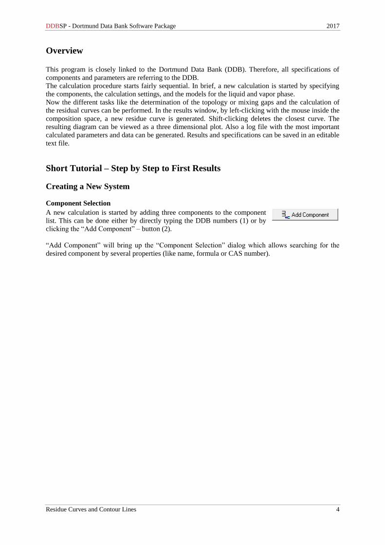
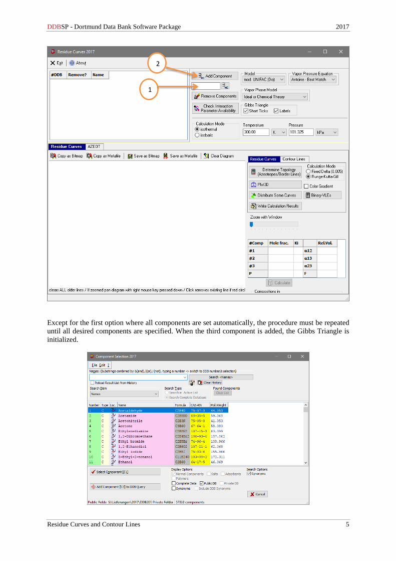
A new calculation is started by adding three components to the component

list. This can be done either by directly typing the DDB numbers (1) or by

clicking the “Add Component” – button (2).

“Add Component” will bring up the “Component Selection” dialog which allows searching for the

desired component by several properties (like name, formula or CAS number).



Except for the first option where all components are set automatically, the procedure must be repeated

until all desired components are specified. When the third component is added, the Gibbs Triangle is

initialized.

1

2



Model Selection

Now the mixture model, vapor pressure equation and vapor phase model have to be selected from the

according drop down menus on the upper right side.

There are two different approaches for calculating liquid phase non-ideality, gE based and equation of

state based models:

gE- models with fitted interaction parameters

o NRTL

o UNIQUAC

o Wilson

Group contribution gE models

o original UNIFAC

o modified UNIFAC (Dortmund)

o modified UNIFAC (Lyngby)

o NIST-modified UNIFAC

Equation of state group contribution models

o PSRK

o VTPR

COSMO based models

o COSMO-RS(Ol)

o COSMO-SAC

o COSMO-SAC2010

o COSMO-SAC2013

Group contribution methods have the advantage that all available group interaction parameters4 are

stored in the DDB. The calculation for several systems can be performed without the need of fitting

model parameters. The mixture property estimation model must be given. If a gE-model is selected,

system specific binary interaction parameters for all component pairs have to be entered.

4 The most current development of the UNIFAC group contribution methods is available from the UNIFAC

consortium. Please visit the consortium web pages (www.unifac.org) for detailed information.



“Edit Parameters” opens a dialog where the parameters can be entered or loaded from the parameter

data bank.

Vapor Pressure Equation

Concerning the vapor pressure the following equations can be chosen:

o Antoine – Best Match

o Antoine – Low

o DIPPR 101

o Wagner 25

o Wagner 36

o Cox



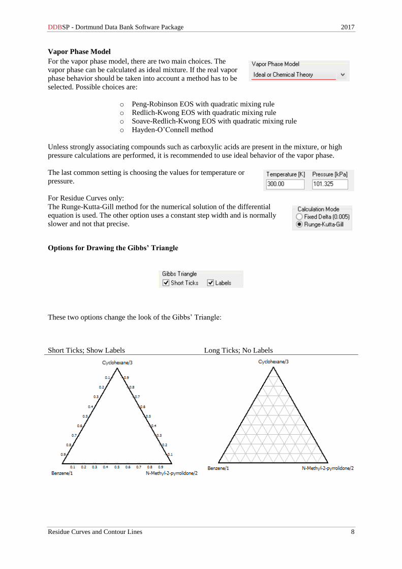
Vapor Phase Model

For the vapor phase model, there are two main choices. The

vapor phase can be calculated as ideal mixture. If the real vapor

phase behavior should be taken into account a method has to be

selected. Possible choices are:

o Peng-Robinson EOS with quadratic mixing rule

o Redlich-Kwong EOS with quadratic mixing rule

o Soave-Redlich-Kwong EOS with quadratic mixing rule

o Hayden-O’Connell method

Unless strongly associating compounds such as carboxylic acids are present in the mixture, or high

pressure calculations are performed, it is recommended to use ideal behavior of the vapor phase.

The last common setting is choosing the values for temperature or

pressure.

For Residue Curves only:

The Runge-Kutta-Gill method for the numerical solution of the differential

equation is used. The other option uses a constant step width and is normally

slower and not that precise.

Options for Drawing the Gibbs’ Triangle

These two options change the look of the Gibbs’ Triangle:

Short Ticks; Show Labels Long Ticks; No Labels



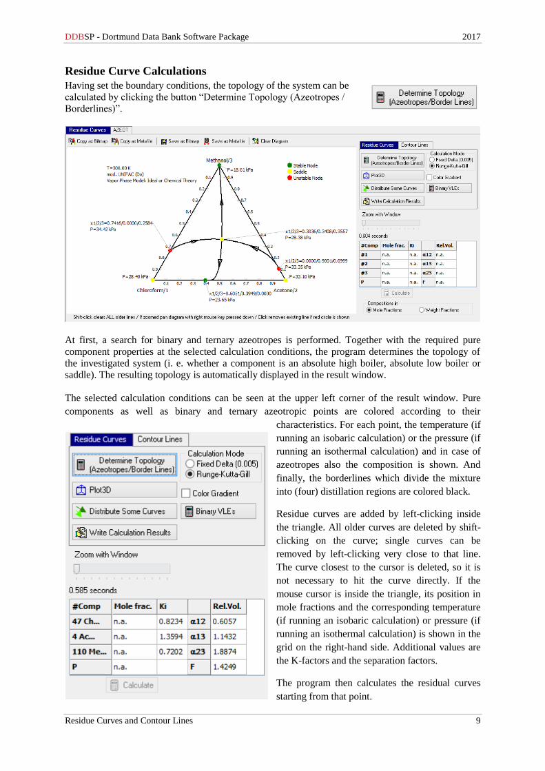
Residue Curve Calculations

Having set the boundary conditions, the topology of the system can be

calculated by clicking the button “Determine Topology (Azeotropes /

Borderlines)”.

At first, a search for binary and ternary azeotropes is performed. Together with the required pure

component properties at the selected calculation conditions, the program determines the topology of

the investigated system (i. e. whether a component is an absolute high boiler, absolute low boiler or

saddle). The resulting topology is automatically displayed in the result window.

The selected calculation conditions can be seen at the upper left corner of the result window. Pure

components as well as binary and ternary azeotropic points are colored according to their

characteristics. For each point, the temperature (if

running an isobaric calculation) or the pressure (if

running an isothermal calculation) and in case of

azeotropes also the composition is shown. And

finally, the borderlines which divide the mixture

into (four) distillation regions are colored black.

Residue curves are added by left-clicking inside

the triangle. All older curves are deleted by shift-

clicking on the curve; single curves can be

removed by left-clicking very close to that line.

The curve closest to the cursor is deleted, so it is

not necessary to hit the curve directly. If the

mouse cursor is inside the triangle, its position in

mole fractions and the corresponding temperature

(if running an isobaric calculation) or pressure (if

running an isothermal calculation) is shown in the

grid on the right-hand side. Additional values are

the K-factors and the separation factors.

The program then calculates the residual curves

starting from that point.



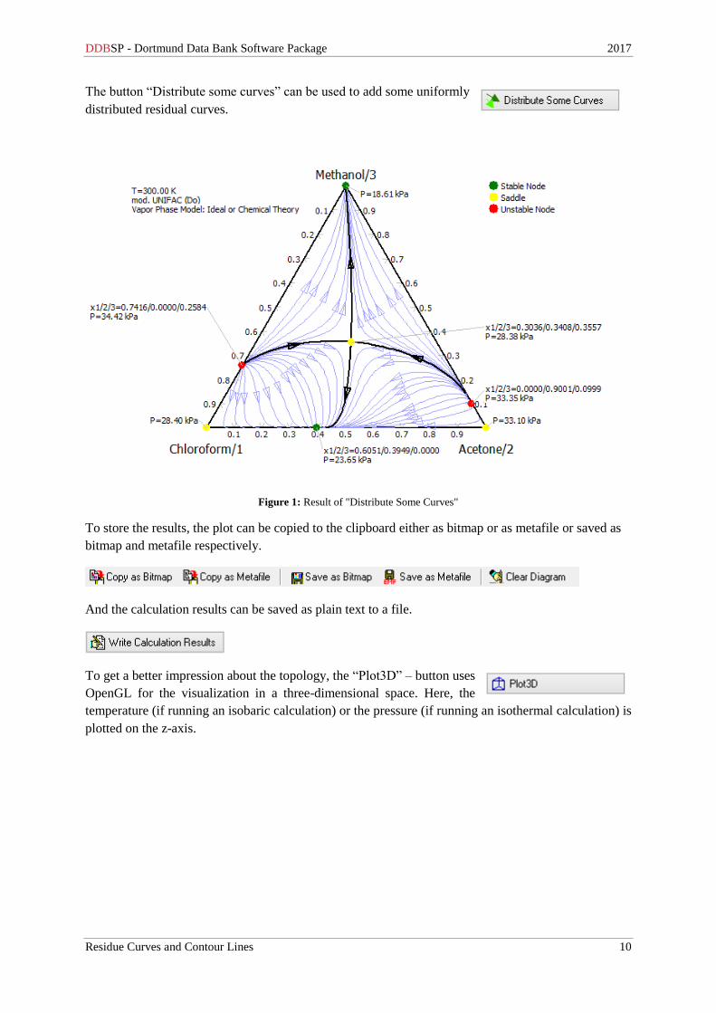
The button “Distribute some curves” can be used to add some uniformly

distributed residual curves.

Figure 1: Result of "Distribute Some Curves"

To store the results, the plot can be copied to the clipboard either as bitmap or as metafile or saved as

bitmap and metafile respectively.

And the calculation results can be saved as plain text to a file.

To get a better impression about the topology, the “Plot3D” – button uses

OpenGL for the visualization in a three-dimensional space. Here, the

temperature (if running an isobaric calculation) or the pressure (if running an isothermal calculation) is

plotted on the z-axis.



The diagram can be rotated with the left mouse key pressed down and moved with the right

mouse key pressed down. The sliders on the right-hand side also allow free rotation of the

plot. Pressing the little buttons above the sliders enables an auto-rotate mode along the

respective axis. The grid may be switched on or off and smooth the lines using the check

boxes. Azeotropes and pure components are represented by little cubes. The color is the same

as in the 2D Plot. The time to display the 3D – plot varies a bit with the amount of data to

display.

The option “Color Gradient” changes the colors of the residual curves and show high pressure

or temperature values in red and low values in blue.



“Clear Diagram” finally clears the diagram without deleting the components and settings and

removing the components from the component list is the precondition to set up a new system.

Contour Line Calculation

The program supports the calculation of contour

lines for the properties

• Separation factor of two components (1-2,

1-3, 2-3)

• K factors for the three components

• Pressure

• Temperature

• 𝐹 = |1 − 𝛼12| + |1 − 𝛼13| + |1 − 𝛼23|

The program supports the calculation of multiple lines with a constant value. In this mode, the

program determines the minimum and maximum values and displays a



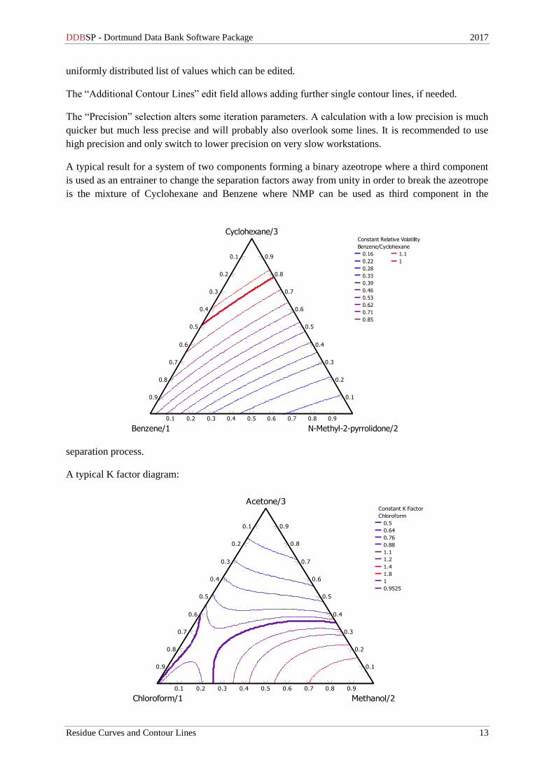
uniformly distributed list of values which can be edited.

The “Additional Contour Lines” edit field allows adding further single contour lines, if needed.

The “Precision” selection alters some iteration parameters. A calculation with a low precision is much

quicker but much less precise and will probably also overlook some lines. It is recommended to use

high precision and only switch to lower precision on very slow workstations.

A typical result for a system of two components forming a binary azeotrope where a third component

is used as an entrainer to change the separation factors away from unity in order to break the azeotrope

is the mixture of Cyclohexane and Benzene where NMP can be used as third component in the

separation process.

A typical K factor diagram:

0.1 0.9

0.1

0.2 0.8

0.2

0.3 0.7

0.3

0.4 0.6

0.4

0.5 0.5

0.5

0.6 0.4

0.6

0.7 0.3

0.7

0.8 0.2

0.8

0.9 0.1

0.9

Chloroform/1 Methanol/2

Acetone/3

0.1 0.9

0.1

0.2 0.8

0.2

0.3 0.7

0.3

0.4 0.6

0.4

0.5 0.5

0.5

0.6 0.4

0.6

0.7 0.3

0.7

0.8 0.2

0.8

0.9 0.1

0.9


Acetone/3Constant K Factor

Chloroform

0.5

0.64

0.76

0.88

1.1

1.2

1.4

1.8

1

0.9525

0.1 0.9

0.1

0.2 0.8

0.2

0.3 0.7

0.3

0.4 0.6

0.4

0.5 0.5

0.5

0.6 0.4

0.6

0.7 0.3

0.7

0.8 0.2

0.8

0.9 0.1

0.9

Benzene/1 N-Methyl-2-pyrrolidone/2

Cyclohexane/3

0.1 0.9

0.1

0.2 0.8

0.2

0.3 0.7

0.3

0.4 0.6

0.4

0.5 0.5

0.5

0.6 0.4

0.6

0.7 0.3

0.7

0.8 0.2

0.8

0.9 0.1

0.9

Benzene/1 N-Methyl-2-pyrrolidone/2

Cyclohexane/3Constant Relative Volatility

Benzene/Cyclohexane

0.16

0.22

0.28

0.33

0.39

0.46

0.53

0.62

0.71

0.85

1.1

1



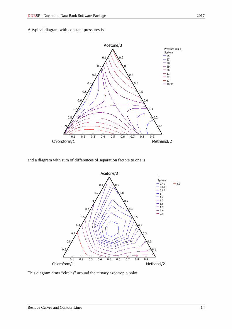
A typical diagram with constant pressures is

and a diagram with sum of differences of separation factors to one is

This diagram draw “circles” around the ternary azeotropic point.

0.1 0.9

0.1

0.2 0.8

0.2

0.3 0.7

0.3

0.4 0.6

0.4

0.5 0.5

0.5

0.6 0.4

0.6

0.7 0.3

0.7

0.8 0.2

0.8

0.9 0.1

0.9


Acetone/3

0.1 0.9

0.1

0.2 0.8

0.2

0.3 0.7

0.3

0.4 0.6

0.4

0.5 0.5

0.5

0.6 0.4

0.6

0.7 0.3

0.7

0.8 0.2

0.8

0.9 0.1

0.9


Acetone/3Pressure in kPa

System

25

27

28

29

30

31

32

33

28.38

0.1 0.9

0.1

0.2 0.8

0.2

0.3 0.7

0.3

0.4 0.6

0.4

0.5 0.5

0.5

0.6 0.4

0.6

0.7 0.3

0.7

0.8 0.2

0.8

0.9 0.1

0.9


Acetone/3

0.1 0.9

0.1

0.2 0.8

0.2

0.3 0.7

0.3

0.4 0.6

0.4

0.5 0.5

0.5

0.6 0.4

0.6

0.7 0.3

0.7

0.8 0.2

0.8

0.9 0.1

0.9


Acetone/3F

System

0.41

0.68

0.87

1

1.2

1.3

1.5

1.9

2.4

2.9

4.2



Prediction of Azeotropic Points

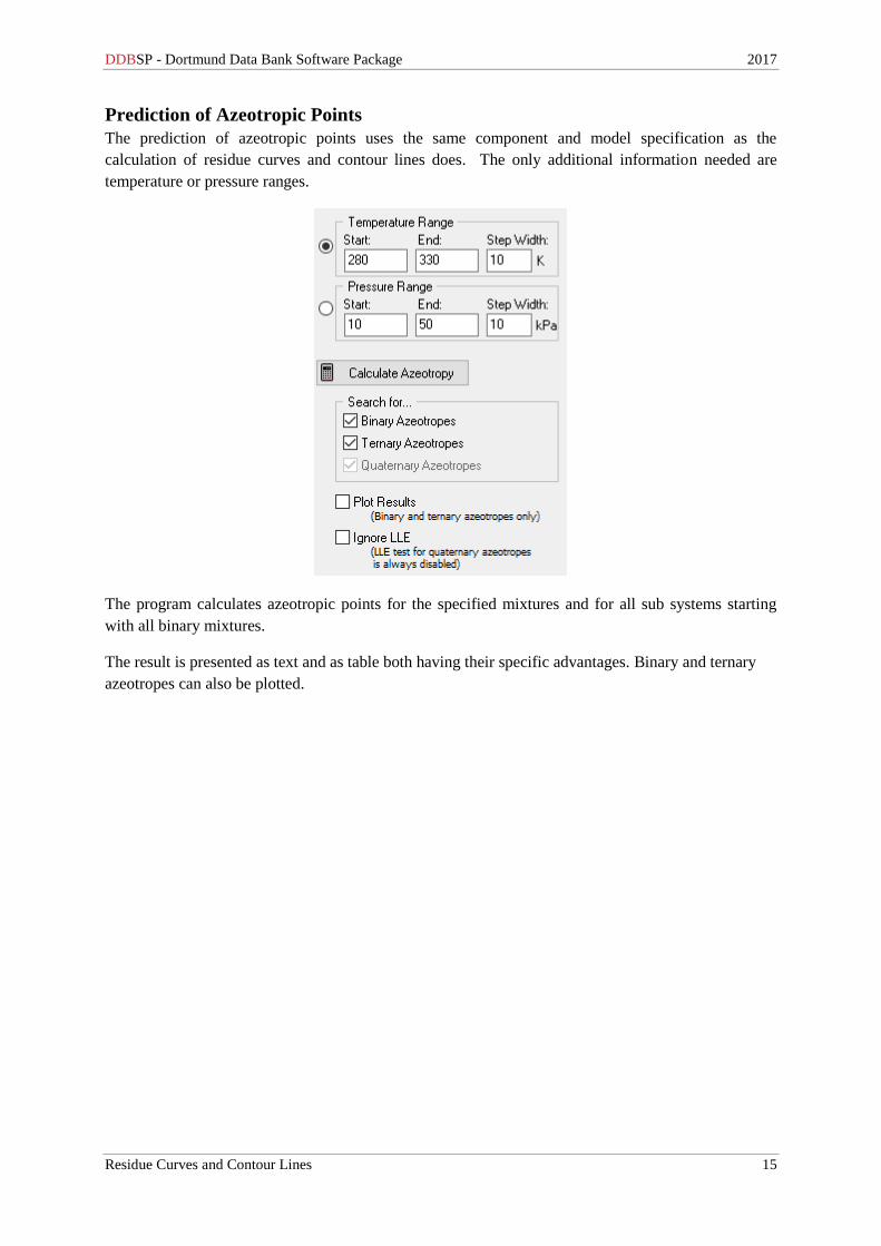
The prediction of azeotropic points uses the same component and model specification as the

calculation of residue curves and contour lines does. The only additional information needed are

temperature or pressure ranges.

The program calculates azeotropic points for the specified mixtures and for all sub systems starting

with all binary mixtures.

The result is presented as text and as table both having their specific advantages. Binary and ternary

azeotropes can also be plotted.

Residue Curves - Contour Lines - Azeotropic Points€¦ · Residue Curves - Contour Lines -...

Documents

Transcript of Residue Curves - Contour Lines - Azeotropic Points€¦ · Residue Curves - Contour Lines -...