Residual Trapping of Carbon Dioxide - Stanford University

Residual Trapping of Carbon Dioxide

Investigations in Geologic Carbon Sequestration: Multiphase Flow of CO2 and Brine, Leak Remediation, and Monitoring

Annual Report 2009

Sally M. Benson, Ariel Esposito, Boxiao Li, Michael Krause, Sam Krevor, Chia-Wei Kuo and Lin Zou

Department of Energy Resources Engineering School of Earth Sciences

Stanford University

April 30, 2010

Contacts Sally M. Benson: [email protected] Boxioa Li: [email protected] Sam Krevor: [email protected] Michael Krause: [email protected] Chia-Wei Kuo: [email protected] Ariel Esposito: [email protected]

mailto:[email protected]�




Abstract

The goal of our research program is to develop reliable methods for predicting the long term fate and transport of CO2 sequestered in aquifers. Our research focuses on developing a robust fundamental science underpinning multiphase flow in saline aquifers. Our focus on saline aquifers is motivated by the generally accepted conclusion that saline aquifers have the largest sequestration capacity, as compared to oil and gas reservoirs or deep unminable coal beds. Saline aquifers are also more broadly distributed and thus, closer to more emission sources. However, unlike oil and gas reservoirs with proven seals that have withstood the test of time, saline aquifers must be carefully characterized to assure that CO2 will achieve high retention rates. Improved fundamental understanding of multi-phase flow and trapping in CO2-brine systems will be needed to take advantage of this large storage capacity of saline aquifers. Additionally, should CO2 leak out of the sequestration aquifer and enter a drinking water aquifer, methods to remediate the aquifer must be available.

Important questions remain to be answered, such as, what fraction of the pore space will be filled with CO2, what will be the spatial extent of the plume of injected CO2, how much and how quickly will CO2 dissolve in brine, and how much CO2 will be trapped by capillary forces when water imbibes back into the plume and to what extent is capillary trapping permanent? How quickly and by which methods can CO2 leakage into shallow drinking water aquifers be remediated? What are the necessary properties of seals? And, if CO2 is leaking how can detect this, either deep in the surface or at the land surface. Here we are developing new experimental data and carrying out simulations to improve our ability to answer these questions. As our research progresses, we will assess which, if any, modifications to currently accepted multiphase flow theory are needed and to develop approaches for reliably predicting field-scale performance.

This year we have made significant progress in a number of areas, specifically:

1. Continued to refine and enhance methods for simulating core-scale experiments, in particular, developing a new method for estimating sub core-scale permeability values;

2. Improved the accuracy of porosity and saturation measurements through fine-tuning the scanning parameters;

3. Improved the degree of quantification of mass balances in the multi-phase flow experiments through the addition of a separator with a Doppler fluid level sensor;

4. Quantified the conditions under which viscous, gravitational and capillary forces control migration of CO2 and brine, including establishing the principle processes by which multi-phase flow displacements depend on flowrate;

5. Initiated modifications to GPRS to enable simulation of fluid flow in rocks with capillary heterogeneities—with the ultimate goal of performing rapid forward modeling, inverse modeling and optimization under these conditions;

6. Developed understanding of the primary challenges to remediate CO2 leakage into groundwater, including approaches to optimize extraction efficiency; and

7. Developed a new method for detecting leakage at the ground surface based on 12C and 13C isotopes on a mobile platform.

Contacts Sally M. Benson: [email protected] Boxioa Li: [email protected] Sam Krevor: [email protected] Michael Krause: [email protected] Chia-Wei Kuo: [email protected] Ariel Esposito: [email protected]





Introduction and Overview

Carbon dioxide capture and sequestration (CCS) in deep geological formations has emerged over the past fifteen years as an important component of the portfolio of options for reducing greenhouse emissions. Four commercial projects now operating provide valuable experience for assessing the efficacy of CCS—sequestering about 4-5 Mt of CO2 annually. If CCS is implemented on the scale needed for large reductions in CO2 emissions, a billion tonnes or more of CO2 will be sequestered annually—a 200 fold increase over the amount intentionally sequestered annually today. Effectively sequestering these large volumes will require building a strong scientific foundation of the coupled hydrological-geochemical-geomechanical processes that govern the long term fate of CO2 in the subsurface. In addition, we will need methods to characterize and select sequestration sites, subsurface engineering to optimize performance and cost, safe operations, monitoring technology, remediation methods, regulatory oversight, and an institutional approach for managing long term liability.

Our research focuses on the fundamental science underpinning sequestration in saline aquifers. Saline aquifers have the largest sequestration capacity, as compared to oil and gas reservoirs or deep unminable coal beds. Saline aquifers are also more broadly distributed and thus, closer to more emission sources. However, unlike oil and gas reservoirs with proven seals that have withstood the test of time, saline aquifers must be carefully characterized to assure that CO2 will achieve high retention rates. Improved fundamental understanding of multi-phase flow and trapping in CO2-brine systems will be needed to take advantage of this large storage capacity of saline aquifers. Important questions remain to be answered, such as, what fraction of the pore space will be filled with CO2, what will be the spatial extent of the plume of injected CO2, how much and how quickly will CO2 dissolve in brine, and how much CO2 will be trapped by capillary forces when water imbibes back into the plume and to what extent is capillary trapping permanent? How quickly and by which methods can CO2 leakage into shallow drinking water aquifers be remediated? What are the necessary properties of seals? And, if CO2 is leaking how can detect this, either deep in the surface or at the land surface. Here we are developing new experimental data and carrying out simulations to improve our ability to answer these questions. As our research progresses, we will assess which, if any, modifications to currently accepted multiphase flow theory are needed and to develop approaches for reliably predicting field-scale performance.

Our laboratory is carrying out core-scale multi-phase flow experiments and reservoir-scale simulations to investigate the fundamental processes that underpin these questions. We are conducting transient and steady state core-flood experiments at representative reservoir pressure and temperatures. Each set of experiments involves co-injecting CO2 and brine at a range of fractional flows and a number of different total flow rates. X-ray CT scanning is used to map the spatial distribution of CO2 and brine. Detailed petrophysical analysis of the core is used to obtain 3-dimensional maps of porosity, permeability and capillary pressure. Rock properties are used to provide insight into the influence of spatial heterogeneity on the distribution of CO2 and brine in the cores. Rock properties are also used as input to carry out high resolution numerical simulations of the core flood experiments. In addition, traditional steady state relative permeability measurements have been made during drainage and imbibition. As our research progresses, we will assess which, if any, modifications to multiphase flow theory are needed to replicate the experiments and develop approaches for up-scaling laboratory measured relative permeability curves for use in reservoir-scale simulations.

Reservoir scale simulations are also being conducted to identify the coupled multi-phase flow and phase behavior that will occur in shallow aquifers, where CO2 exists as a gas phase. These simulations are used to assess and evaluate options for remediating shallow groundwater, should some CO2 escape from the storage reservoir and migrate into drinking water aquifers. As discussed in this report, the complex interplay between multiphase flow, buoyancy, dissolution,

exsolution and relative permeability/capillary pressure hysteresis results in surprising spatial and temporal dynamics that hamper, to some degree, the ability to quickly extract shallow plumes of CO2.

Illustration of the 4 interrelated components of our approach to study multiphase flow and trapping in saline aquifer. This report has five sections. Section 1 describes the approach we are taking for the sub-core scale characterization of porosity, permeability and capillary pressure that is needed as input for simulating the core-scale experiments. Section 2 describes the simulations of the laboratory experiments, including the effects of gravity, heterogeneity and capillary pressure. Section 3 describes the development of a new capability for simulating capillary heterogeneity in Stanford’s General Purpose Reservoir Simulator (GPRS). Section 4 describes early results from simulations of remediating CO2 plumes in shallow groundwater aquifers. Section 5 describes our new method for detecting CO2 leakage at the ground surface.

• Reliable methods for permeability mapping at the sub-core scale

• Reliable methods for capillary pressure mapping

• Theoretical foundation for observed multi-phase flows

• Parametric formulation for rate dependent relative permeability curves

PetrophysicalCharacterization

Core-Scale Multiphase Flow Experiments

Multiphase Flow Theory

NumericalSimulation

• Influence of heterogeneity on multi-phase flows

• Flow-rate dependence of CO2 saturations and relative permeability

• Flow history dependence• Residual gas trapping• Mobility of exsolved CO2

• History matching experiments

• Sensitivity analysis• Simulation artifacts• Implication for large

scale processes

• Reliable methods for permeability mapping at the sub-core scale

• Reliable methods for capillary pressure mapping

• Theoretical foundation for observed multi-phase flows

• Parametric formulation for rate dependent relative permeability curves




NumericalSimulation




NumericalSimulationNumericalSimulation

• Influence of heterogeneity on multi-phase flows

• Flow-rate dependence of CO2 saturations and relative permeability

• Flow history dependence• Residual gas trapping• Mobility of exsolved CO2

• History matching experiments

• Sensitivity analysis• Simulation artifacts• Implication for large

scale processes

2. Permeability Models for Numerical Simulation of Core Flooding Experiments Michael Krause and Sally M. Benson. Abstract

The 2007 and 2008 reports discuss one of the main objectives of this research group’s goals, which is to be able to numerically replicate a core flooding experiment. More specifically, we want to prove the ability to replicate using numerical simulation, the experimentally measured sub-core scale CO2 saturation values and spatial distribution of these values. The workflow for this is procedure is to conduct a core flooding relative permeability experiment, as described in the 2007 and 2008 annual reports, then to use the exact same conditions in a multiphase flow numerical simulator to predict the spatial distribution of CO2 as measured by medical CT scanning during the core flooding experiment.

The ability to replicate these results is important as a proof of concept of our ability to predict subsurface CO2 distributions in applications such as CO2 sequestration, and enhanced oil recovery. It is also a useful tool for experimenting with different physical parameters which control the distribution of fluids, and studying which parameters are important under various flow regimes and conditions. This section briefly describes the procedure for conducting these simulations, and shows the results of the most recent efforts to match the measured saturation distributions. See the 2007 and 2008 reports for more detail and the results of past efforts. Numerical Simulation Methodology

Numerical simulations of the core flooding experiment require four main experimental data inputs at two different scales: sub-core scale porosity, sub-core scale capillary pressure, whole core relative permeability, sub-core scale permeability, and the sub-core scale saturation measurements we are attempting to replicate numerically. The sub-core scale porosity and saturation measurements are taken at the sub-mm scale by the CT scanner during the core flooding experiment. The whole core relative permeability is also calculated during the experiment.

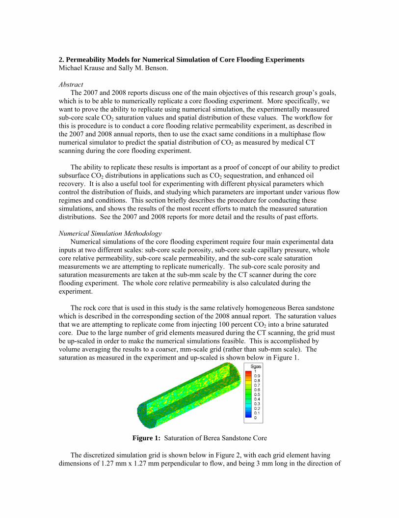
The rock core that is used in this study is the same relatively homogeneous Berea sandstone which is described in the corresponding section of the 2008 annual report. The saturation values that we are attempting to replicate come from injecting 100 percent CO2 into a brine saturated core. Due to the large number of grid elements measured during the CT scanning, the grid must be up-scaled in order to make the numerical simulations feasible. This is accomplished by volume averaging the results to a coarser, mm-scale grid (rather than sub-mm scale). The saturation as measured in the experiment and up-scaled is shown below in Figure 1.

Figure 1: Saturation of Berea Sandstone Core

The discretized simulation grid is shown below in Figure 2, with each grid element having

dimensions of 1.27 mm x 1.27 mm perpendicular to flow, and being 3 mm long in the direction of

flow. The injection rate of CO2 in the experiment was intentionally selected to be high enough to overcome the effects of gravity, caused by density differences between CO2 and brine, which is around 1 ml/min for a homogeneous core. The injection rate used in this experiment and series of simulations is 3 ml/min of H2O saturated supercritical CO2. The temperature and pressure are 50°C and 12.41 MPa (1800 psi), to ensure the CO2 remains in supercritical state.

Figure 2: Simulation Grid of Berea Core (grid element size is 1.27 mm x 1.27 mm x 3 mm) Sub-Core Scale Porosity

The sub-core scale porosity is easily measured during the core-flooding experiment using the CT scanner. Similarly to the saturation grid, this data was also upscaled by volume averaging fine scale measurements onto a coarser grid, and is shown below in Figure 3. The porosity values in the figure are directly input into their spatially corresponding grid elements in the simulation grid in Figure 2.

Figure 3: Porosity of Berea Sandstone Core

Whole Core Relative Permeability

Relative permeability from the experiment can be calculated using Darcy's Law in Eq. 1 below, where qi is the injection flow rate of phase i, μi is the viscosity of phase i, L is the length of the core, k is the absolute permeability of the whole core, A is the cross sectional area of the core, and ΔP is the pressure drop measured across the core. This calculation is done for the CO2 and brine phases, to yield the relative permeability data for different combinations of flow rates of each phase, called fractional flows, to get the experimental measurement in Figure 4. This procedure is described in more detail in the 2007 Annual Report. Relative permeability is a core-average property according to conventional treatment, and is not unique to each grid element.

Figure 4 also shows the curve fits to the data for each phase used in the numerical simulation. The fits were obtained by history matching the core average pressure drop and saturation for a homogeneous core with core-average properties. Therefore, although the fits do not appear to match the data points, the numerical results for a homogeneous core are accurate when using these curves.

(1)

Figure 4: Relative Permeability Experiment Data and Curve Fit

Sub-Core Scale Capillary Pressure

Capillary pressure cannot be measured by conventional means at the sub-core scale shown in Figure 2. A useful method for translating a single, core-average capillary pressure measurement to the sub-core scale is the Leverett J-Function, shown in Eq. 2 (Leverett, 1942):

(2)

where Pc is the capillary pressure which exists between two immiscible fluid phases, σ is the interfacial tension, θ is the contact angle between the fluid interface and the rock surface, ϕ is the porosity, k is the permeability and J(Sw) is and empirical Leverett J-Function, which is itself a function of the wetting phase saturation, Sw. The interfacial tension is calculated to be 0.0285 dynes/cm from Chalbaud et al. (2008) and the contact angle is assumed to be 180 degrees.

Eq. 2 is implemented by taking a single capillary pressure measurement on a representative sample from the whole core, fitting the measured data with Eq. 2 using a dimensionless empirical J-Function, and then scaling that measured J-Function to the sub-core scale grid element porosity and permeability, to get a unique capillary pressure curve for each grid element. The J-Function has several common forms, but is itself an empirical function used to fit a measured capillary pressure curve (see 2008 Annual Report for measurement details). The function used in this study is from Silin et al. (2009), and is shown in Eq. 3.

(3)

where A, B, λ1, and λ2 are empirical fitting parameters, and S* is the normalized wetting phase (brine) saturation, given by Eq. 4.

(4)

where Swr is the residual or irreducible wetting phase saturation, which is the absolute minimum wetting phase (brine) saturation which can be reached by physical multiphase flow displacement processes.

Eqs 3 and 4 are then combined and used to fit measured experimental data, shown below in

Figure 5. The fits use the whole-core average porosity and permeability in Eq. 2, since the experimental measurement was made on a representative sample from the experiment core (which has known average porosity and permeability from measurements). Two data fits are used, Curve Fit 1 & 2, using slightly different fitting parameters, but of the same general characteristic shape. The complicated shape of the curve prevents an exact match, however, the fits are relatively good over the domain of the data.

Figure 5: Capillary Pressure Curve Fits

The most important aspect of the Leverett J-Function scaling is that the J-Function is

expected to be the same for all samples from the same rock type. Therefore, if a different rock core from the same source rock were used but had different permeability and porosity, the J-Function fitting parameters would be the same, and could be used from this measurement in Eq. 3 and scaled to the other core porosity and permeability according to Eq. 2, to get the correct capillary pressure curve for the other rock core. This concept is important because it also applies at the sub-core scale within the host rock, meaning that once the J-Function fitting parameters are known for the core in this study, unique capillary pressure curves can be created for each grid element in Figure 2 by scaling the generic J-Function to each grid elements' unique porosity and permeability. Sub-Core Scale Permeability

Permeability cannot be measured non-destructively at the sub-cores scale, and must be calculated using an equation linking it to some other measured sub-core scale parameter. The two directly measured sub-core scale parameters are porosity and saturation. While permeability is a physical parameter required to model flow in porous media, Eq. 2 shows that it is also required in order to scale the J-Function to get the unique capillary pressure curve for each element in the core. Therefore, permeability has a dual function in these numerical simulations.

Methods to calculate sub-core scale permeability have been at the center of this work since it was started, and the 2007 and 2008 reports showed that very simple methods which use well established laws relating permeability to porosity were simply not adequate. These methods were desirable because the unique values of porosity are precisely known from the CT measurements for each sub-core scale grid element. These simple porosity laws are routinely used at the whole-

core scale, however, their application to the sub-core scale was shown to be inconsistent with their whole-core scale properties, and shown to yield sub-core saturation results which do not correlate with the measured values.

In order to overcome this, a new approach was taken, which takes advantage of the other directly measured sub-core scale dataset, saturation. It is evident that permeability and saturation are related, through the capillary pressure, shown by Eqs. 2 and 3. One very important assumption which can be mathematically derived, is that the capillary pressure after the saturation and pressure drop have reached steady-state (are constant), is constant throughout the rock core if there are no capillary barriers and the flow is dominated by viscous forces (which will be true at high flow rates).

With this assumption, we can use the core average saturation, core average porosity and core average permeability, and the J-Function fitting parameters used to make the curves fits in Figure 5 to calculate the capillary pressure using Eqs. 2 and 3. After this, the only sub-core scale property in Eq. 2 which is unknown is permeability. Rearranging Eqs. 2 & 3 to solve for each unique grid element i's permeability gives Eq. 5.

( )[ ] ( )( )22,2 cos1 θσφ ⋅= iwi

ci SJ

PSk (5)

where is the core average capillary pressure at the core average saturation at steady-state flow, J(Sw,i) is the J-Function for element i in Figure 2, evaluated using the fitting parameters used for the curve fits in Figure 5, and the measured saturation for grid element i. Numerical Simulation Results

The numerical simulator TOUGH2-MP with the ECO2N module was used to perform the numerical simulations. In TOUGH2-MP, the J-Function must be defined using the fitting parameters, that is, it cannot be entered as tabular data from the measurement, therefore, the fit will not be perfect, as shown in Figure 5. However, it is possible to use the tabular data to calculate permeability by using a cubic spline curve fit to the data, and evaluating the spline at each grid blocks measured saturation to get the J-Function value. It was not known which approach would be better for calculating permeability, therefore, several methods were used. The experimental conditions and other simulation input is summarized for reference in Table I. Table I: Summary of Experimental and Simulation Conditions

Simulation Conditions Thermophysical Data Injection Conditions Simulation Grid Data T (˚C) 50 Dissolved CO2

init (mass fraction) 0.04873 qCO2-Gas (kg/s) 3.03E-05 Simulation Cells 62712

P (MPa) 12.41 ρCO2 (kg/m3) 608.38 qCO2-Aq (kg/s) 0.00E+00 Cell Length (mm) 3

xNaCl (ppm) 6500 ρH2O (kg/m3) 993.33 qH2O-Gas (kg/s) 1.17E-07 Cell Width (mm) 1.27

φave 0.185 σCO2-Brine (N/m) 0.0285 qH2O-Aq (kg/s) 0.00E+00 Longitudinal Upscaling 2:1

kave (md) 85 Injection Rate (ml/min) 3 qNaCl (kg/s) 0.00E+00 In-Slice Upscaling 5:1

A total of three simulations were run using the capillary pressure method for calculating permeability. The first simulation uses Curve Fit 1 in Eq. 5 to calculate permeability, and in the simulation for capillary pressure, the second uses the experimentally measured data in Figure 5 to calculate permeability in Eq. 5, and Curve Fit 1 in the simulation for capillary pressure, and the third simulation uses Curve Fit 2 for permeability and in the simulation. A summary of the results is shown in Table II, with a single slice, 33, near the middle of the core shown for visual comparison, however the same results are consistent for all slices.

The table shows that the resulting permeability grids, and saturation distributions vary little between the three simulations, with a higher standard deviation of the saturation histogram for Curve Fit 2 than Curve Fit 1 or the discrete data permeability calculations. The table also shows that a visual comparison of the three simulations with the experimental result is relatively good. The degree of contrast in CO2 saturation is not as high in the simulations as the experiment, but the qualitative match is quite good. For comparison, the "best" match using the simple porosity based equation in Eq. 6 (Pape et al., 2000) to calculate permeability is also shown. The visual match between this result and the experiment is not nearly as good as the capillary pressure methods, and the standard deviation of the saturation distribution within the core is also much smaller than the experiment, even for this "best" porosity model.

(6) In order to compare how well the spatial distribution of saturation in the numerical simulation

matches the experimental measurement, a simple plot of the simulation saturation values vs. the experimentally measured values for slice 33 is shown in Figure 6 (results typical for all slices). A perfect correlation in this figure would fall on the diagonal 1:1 slope line with intercept at zero, shown in blue. The figure shows that the three capillary pressure methods have a unique and specific correlation with the experimental values, although not perfect, but does show a good correlation. However, the figure also shows that there is no spatial correlation between the "best" porosity based method results and the experimental measurements, which is consistent with the conclusions of the 2008 Annual Report findings.

In order to quantify the match, the R2 fit of the sub-core scale spatial saturation values is calculated, as well as the core average saturation and core average pressure drop, and these are compared to the experimental measurement in Table III. The table shows that all of the simulations under predict the pressure drop, and over predict the saturation, but that the capillary pressure based simulations are better than the "best" porosity equation simulation. More importantly, the table shows that the actual prediction of the sub-core scale saturation distribution is statistically significant for each of the capillary pressure-based simulations, with an R2 value of around 0.75. However, the table shows that the porosity-based method simulation actually has a negative R2, indicating that it in fact has no correlation with the experimental saturation measurement, as evident also from Figure 6.

Table II. Summary of Simulation Results

Description Slice Permeability Map

Slice 33 Saturation Map

Whole Core CO2 Saturation Histogram

Experiment Data CO2 Sat. Std. Dev. 0.1564

Simulation 1 Eq. 5 J(Sw) - Curve Fit 1

Sim Pc - Curve Fit 1 CO2 Sat. Std. Dev. 0.0832

Simulation 2 Eq. 5 J(Sw) - Discrete Data


Simulation 3 Eq. 5 J(Sw) - Curve Fit 2


"Best" Porosity-Based Model


Figure 6: Comparison of Numerically Predicted Saturation vs. Experimentally Measured Saturation for Slice 33 Table III: Quantitative Comparison of Simulation and Experimental Results

Experiment 7059 ‐ 0.5026 ‐ ‐1 6609.1 ‐6.373 0.5163 2.730 0.74422 6652.7 ‐5.756 0.5148 2.429 0.73123 6559.3 ‐7.079 0.5161 2.680 0.7790

Porosity 6338.2 ‐10.211 0.5383 7.103 ‐0.1331

SimulationCore ΔP (Pa)

ΔP Error (%)

Core CO2

Saturation

Sat. Error (%)

Sub‐Core CO2

Saturation R2 Fit

Summary and Future Work

This work has shown that using a capillary pressure-based method for predicting permeability yields accurate results when simulating core flooding experiments. The spatial distribution of fluids is accurately predicted, as well as core average saturation and pressure values. The work also shows that these methods are superior in their ability to capture these sub-core scale saturation distributions to simpler porosity-based methods.

Although these results are very promising, additional work is required to further improve the match and to explore the application of these capillary pressure-based techniques for predictive purposes. Future work will involve experimenting with methods to improve the match, and to use saturation maps for different injection conditions on the same core, and try to predict the same saturation distributions. Specifically, the core floods are conducted by injecting increasing fractional flows of CO2 from zero to 1 in steps (from no CO2 injection to 100 percent CO2 injection), if these permeability maps are correct, a saturation map at one step, such as 100 percent CO2 injection as was used in this study, should be able to be used to predict the saturation distribution at a different injection fractional flow, such as 50 percent

CO2 injection. Predictive capabilities such as this will greatly reduce the amount of time required to conduct experiments if fewer data points are needed. Publications Krause, M., Perrin, J-C., and Benson, S. M., 2009. Modeling Permeability Distributions in a Sandstone

Core for History Matching Coreflood Experiments. Proc. SPE International Conference on CO2 Capture, Storage and Utilization. San Diego, CA USA, 2-4 November. Also, submitted for Publication in SPEJ.

References Chalbaud, C., Robin, M., Lombard, J.-M., Martin, F., Egermann, P., and Bertin, H. 2009. Interfacial

Tension Measurements and Wettability Evaluation for Geological CO2 Storage. Advances in Water Resources 32 (1): 98-109

Leverett, M. C. 1942. Dimensional-Model Studies of Oil-Field Behavior. Trans. AIME 146: 175-193

Pape, H., Clauser, C., and Iffland, J. 2000. Variation of Permeability with Porosity in Sandstone Diagenesis Interpreted with a Fractal Pore Space Model. Pure and Applied Geophysics 157: 603-619

Silin, D., Patzek, T., and Benson, S. M. 2009. A Model of Buoyancy-Driven Two-Phase Countercurrent Fluid Flow. Transport in Porous Media 76: 449-469

Contacts

Michael Krause: [email protected]

3. Heterogeneous Core Simulations Chia-Wei Kuo and Sally Benson Abstract

The second part of the numerical simulation work is to interpret and extrapolate the results of core-scale multi-phase flow experiments. This study includes modeling the behavior of brine displacement by injected CO2 in a core-scale laboratory experiment and history-matching laboratory data. Through these numerical studies we will develop a better understanding of the role of sub-core scale heterogeneity, gravity and flow rate on multi-phase flow, particularly in the context of these core-scale laboratory experiments. Experimental Data

A series of steady state multiphase flow experiments at a range of fractional flows and different total flow rates have been conducted using Berea sandstone by Perrin and Benson (2009). The core used in laboratory experiments is 5.08 cm in diameter and 15.24 cm long with a mean porosity of 20.3% and the average absolute permeability of 430±7 mD. CO2 and brine were co-injected into the core at reservoir conditions (Pres=12.4MPa and T=50˚C). X-Ray CT scans of the core prior to injection was used to provide a three dimensional spatial porosity map, which is made up as a stack of 29 lateral images data (159 pixel diameter). Each pixel values represent the porosity at that location. The slice-averaged CT porosity values vary along the core from 19.87% to 20.54%, which is quite uniform (Figure 1). However, there are some important sub-core scale heterogeneities in the three dimensional porosity map (Figure 1), especially, bedding through the core at a high dip angle.

Figure 1: Left: 3D porosity map of the Berea sandstone sample with φ =20.3% and absolutek =430±7 mD. Right: Porosity profile along the sample. Methodology of Numerical Simulation

In order to simulate the laboratory experiments, the core must be replicated in the simulation grids. Here the core was divided into 53× 53× 31 grid blocks (Figure 2) where each grid element has dimensions 0.884mm× 0.884mm× 5.08mm. Therefore a roughly cylindrical simulation grid made of 64,635 rectangular elements was built. The simulation temperature and pore pressure were held constant at 50˚C and 12.4 MPa respectively, which is typical of the reservoir conditions. Before injecting CO2 and brine into the core, all pore-space is filled with water that is in equilibrium with dissolved CO2 and 10,000 ppm NaCl. When CO2 and brine are injected into the core, the brine is partially displaced by CO2. At these initial conditions the mass fraction of dissolved CO2 in brine is 4.8%.

Figure 2: Simulation core of 53× 53× 31 grid blocks The relative permeability relations used in the simulations are the following:

CO w2

2

2

n nw CO ,r w wr

r,CO r,wwrn wr

1-S -S S -Sk = k =

1-S 1-S⎛ ⎞ ⎛ ⎞⎜ ⎟ ⎜ ⎟

⎝ ⎠⎝ ⎠ (1)

Sw is the average brine saturation, Swr is the residual brine saturation, SCO2,r is the residual CO2 saturation, and nw and nCO2 are the functional exponents for the brine and CO2 curves respectively. In this study, SCO2,r is set to zero in all simulations, therefore, there are four free parameters in the relative permeability relations: Swr, Swrn, nw and nCO2. The smallest error between simulations and experiments can be obtained by searching suitable range of these four parameters; using optimization to get values of input parameters shown in Table I. These power-law functions for brine and CO2 are used to fit the relative permeability curves measured from the laboratory experiments (Figure 3) and are used as inputs to the TOUGH2 model. Table I: Input parameter values for relative permeability and capillary pressure curves fit

Parameters of Relative Permeability SCO2,r Swr Swrn nw nCO2

0 0.15 0.15 7 3 Parameters of Capillary Pressure Curve

σ (dynes/cm) A B λ1 λ2 Sp

22.47 0.007734 0.307601 2.881 2.255 0

Figure 3: Relative permeability curves for CO2 and brine fit to experimental data. The capillary pressure of element i, Pc,i, used in this paper is defined as following:

, ( ) ( ) (2 )ic i w w

i

P S J S akφ

σ=

Pc,i is calculated by scaling the new parameterization of J-function by the square root of the element’s porosity, φi and permeability, ki (Leverett scaling), and multiplying by CO2-brine interfacial tension σ. A modified J-function (Silin et al., 2009) which provides a better fit to the laboratory measured capillary pressure curve was used in this simulation work:

2 2

1

1/*

*

1( ) ( -1) (1- ) (2 )wJ S A B S bS

λ λλ= +

*

- (2 )

1-w P

P

S SS c

S=

The capillary pressure curve for each element in the simulation is scaled by the relationship (2a) while the values of input parameters (A, B, λ1, λ2, Sp) are shown in Table 1. Figure 4 shows a plot of Pc,i versus Sw. The match between the measured and fitted curve is very good over the majority of the saturation range, and in particular the saturation range observed in the experiments.

1.E+02

1.E+03

1.E+04

1.E+05

1.E+06

1.E+07

1.E+08

1.E+09

1.E+10

0.0 0.2 0.4 0.6 0.8 1.0

Water Saturation

Cap

illar

y Pr

essu

re (P

a)

Pc Data(Pa)Fitted Curve(Pa)

Figure 4: Laboratory capillary pressure data with curve fit used in simulations

A three dimensional permeability map is generated by using the Kozeny-Carman equation (Kozeny, 1927; Carman, 1937):

3

2 (3)(1- )

ii

ik S φ

φ=

S is a scaling factor assures that the average of all permeability values is equal to the average permeability of the core, 430 mD. φi is a pixel value in the porosity map, and ki is the corresponding value calculated using Eq. 3. Therefore, in heterogeneous case, capillary pressure can be calculated from new Leverett J-function provided the known porosity and permeability data. Each grid element has a unique pair of porosity and permeability values; hence a unique capillary pressure curve.

To determine the effect of heterogeneity and gravity on brine displacement, homogeneous core and heterogeneous core are simulated with identical input parameters. The only difference is for the heterogeneous core, we use measured values of the porosity distribution up-scaled by simple averaging to the size of the grid shown in Figure 2. The flow rate effect and gravity effect are evaluated for both

homogeneous and heterogeneous cores. The simulations presented here focus on the 95% fractional flow of CO2 and 5% brine.

The range of flow rates is chosen from 1.2 ml/min to 0.001 ml/min (four orders of magnitudes). In

the laboratory, flow velocity can be calculated based on volumetric flow rates and core cross section. Consider a homogeneous reservoir with a thickness of 100 meter and an injection well with injection rate of 1 Mt CO2/yr; we can then calculate the flow velocity as a function of distance from the well using a 1-D radial geometry. For example, figure 5 shows that laboratory flow rate 1.2 ml/min corresponds to CO2 plume at 4.2 meter away from the injection well; 0.1 ml/min corresponds to 100 meter away and 0.01 ml/min corresponds to 1 kilometer away. Therefore these flowrates span the range of conditions expected in the near-will region to leading of the plume, which may be up to 5 km or more from the injection well. Based on this reasoning, the interplay of viscous, capillary and gravity forces in core flood experiments are investigated at different Gravity and Capillary numbers representative of those expected for a typical sequestration project.

Figure 5: The volumetric flow rate and its corresponding distance of CO2 plume at the reservoir (100 meter thickness and 1 Mt CO2/yr injection rate)

The Capillary Number (Ca) is defined as a dimensionless number that relates the magnitude of the capillary force to the viscous force:

(4)t wuCa

μσ

= ut is the total average Darcy flow velocity and μw the viscosity of brine. The Gravity Number (Ngv), or

ratio of gravity to viscous force, is defined by Zhou et al. (1994) as

2

(5)gvco t

gkLNH uρμ

Δ=

Δρ is the density difference between CO2 and brine, g the acceleration of gravity, L the length of the core, H the height of the core, and μCO2 the viscosity of CO2. In our simulations, capillary number is around 10-

6 to 10-10. Therefore, for the CO2/brine systems, for all but the near-well region, displacements are dominated by capillary and buoyancy. Simulation Results Average CO2 Saturation

We first consider the average saturation of the core as a function of capillary and gravity number after steady state is achieved. The steady state saturation of CO2 as a function of capillary number Ca and gravity number Ngv is shown in Figure 6. Steady state is generally reached after injecting 3-5 pore volumes of fluids and most of the simulation results are running after at least 10 pore volumes. The

values of Ca and Ngv are only controlled by varying injection rates. Low Ca and high Ngv, representative of the leading of the plume while high Ca and low Ngv, representative of the near well region. For the homogeneous case without considering buoyancy, CO2 saturation is 0.324 for the case 95% CO2 injection based on Buckley-Leverett theory. Figure 6 shows that the simulation results match the theoretical value.

For those simulations including gravity, the efficiency of brine displacement during vertical

displacement falls into three separate regimes. At high flow rates or viscous dominated regime (regime I) which corresponding to capillary number Ca ≥ 10-7 and gravity number Ngv ≤ 2, the brine displacement efficiency is nearly independent of flowrate. When the capillary number drops below 10-7 or Ngv > 2 (gravitational dominated regime, or regime II), homogenous cores display flow rate dependent saturation distributions, with brine displacement efficiency dropping by about 80%. At very low capillary numbers Ca ≤ 2x10-9 or Ngv > 100 (capillary dominated regime or regime III), the brine displacement efficiency appears to asymptotically approach an even lower saturation.

Figure 6: Carbon dioxide saturation as a function of capillary number and gravity number

Figure 6 compares the brine displacement efficiency between the homogeneous core with and without gravity. If we add heterogeneous properties into the core, does this flow rate effect still exist? Figure 7 shows the simulations for the heterogeneous cores compared to the homogeneous one. Both the heterogeneous and homogeneous cores display flow rate dependent saturation distributions when including gravity with the average saturation dropping from about 32% at the highest rates to less than 10%. The decrease in brine displacement efficiency is only slightly smaller for heterogeneous cores with buoyancy. The decreasing trend of brine displacement efficiency changes gradually over two orders of magnitude of flow rate (0.01-1 ml/min) when including gravity. For the cases with rock heterogeneity and no gravity forces, the transition zone from high efficiency to low efficiency displacements is abrupt, occurring at a capillary number of about 3× 10-9 (Figure 7). In the capillary dominated regime, the displacement efficiency is strongly dominated by the heterogeneity of the rock.

Figure 7: Comparison of heterogeneous and homogeneous cores with and without gravity

Simulated CO2 Saturation Distributions In addition to measuring the average saturation of the core, we can also measure is the saturation

distribution. For uniform core with no gravity, the CO2 saturation distribution is uniform and equal after steady state for every flow rate. Moreover, saturation gradients only occur along the horizontal direction during the transient period while the front is advancing through the core, and shortly thereafter when the fractional is approaching the fractional flow at the inlet. However, once gravity is included, the distribution map changes significantly.

Figure 8 compares the saturation distribution for the homogeneous case and heterogeneous case. It

shows that not only does the average brine efficiency decrease when flow rates are lower, but the distribution also changes. In the viscous dominated regime, the capillary pressure is uniform along the vertical and horizontal axes of the core. The average saturations are accurately predicted based on Buckley-Leverett theory which neglects capillarity and gravity. The saturation varies widely throughout the core, with low porosity portions having low saturations and high porosity saturations having higher saturation of CO2. In addition, the saturation gradient is very small and only in the vertical direction due to density difference between CO2 and brine. In the gravitational dominated regime, saturation gradients occur along both vertical and horizontal directions. In this regime, the presence of heterogeneity increases the flow rate dependency; however, buoyancy appears to be the major factor leading to the flow rate dependence. In the capillary dominated regime, capillary pressure gradients control displacement of the fluids, tending towards achieving capillary-gravitational equilibrium based on the capillary pressure curve of the core.

When comparing the saturation distribution between the homogenous and heterogeneous cores, it is evident that the combination of gravity and heterogeneities controls CO2 distribution in the simulations. The decrease of brine displacement efficiency for the homogeneous cores from high flow rate 1.2 ml/min to low flow rate 10-3 ml/min is around 80% while the decrease of brine displacement efficiency due to the heterogeneity is an additional 30%.

Comparison between Measured and Simulated CO2 Saturation Distributions Figure 9 shows the measured CO2 saturation distribution (Perrin and Benson, 2009) at a fractional

flow of 100% CO2 at total flow rate 1.7 ml/min and a 3D porosity map. Experiments conducted in this viscous dominated regime are consistent with the simulations presented here. Large variations in saturation are observed and can be simulated reasonably well with models including the effects of viscous, capillarity and buoyancy forces. However, the measured contrast in the saturation is much greater than the simulated contrast. It has been shown by Krause et al. (2009) that porosity based models of permeability are not reliable for determining sub-core scale permeability variation. In particular, the contrast in permeability is too small.

Improved methods for estimating sub-core scale permeability variations are needed to improve the

quantitative agreement between measured and simulated saturation distributions. Therefore, the alternative empirical rock property model which can replicate the observed saturation distributions much better than Kozeny-Carman model is using as follows:

4exp( )ii m nk ϕ= × + , m=64, n=-6 (6) Figure 10 compares the brine displacement efficiency between these two models. The higher the

degree of heterogeneity in the core, the more quickly the displacement efficiency deviates from the homogeneous model. Also, the greater the heterogeneity, the lower the average saturation. At high and

low capillary numbers, the difference of brine displacement efficiency between the homogeneous and heterogeneous systems is small, while it is very significant in the transient between these two regimes.

Figure 8: Saturation distribution for homogeneous and heterogeneous cores with gravity.

Figure 9: CO2 saturation for 100% CO2 at 1.7 ml/min flow rate (left) and porosity map (right).

Figure 10: Comparison of brine displacement efficiency for two porosity-permeability models with gravity

Figure 11 shows these two models: second column is the Kozeny-Carman model and the third column is high contrast model. In order to easily compare the measured CO2 saturation distribution, the scale of color bar is from 0 to 1 rather than 0.05 to 0.33. Both simulations replicate the spatial patterns measured in the experiment. However, the high contrast model more closely replicates the measured saturation distribution. The greater the permeability contrast, the closer the match between the simulated and experimental results. The higher the degree of contrast in rock properties results in the greater contrast in saturation. In particular, the influence of high and low porosity layers on the CO2 saturation is closely replicated. However, as shown, the CO2 saturations in the high porosity layers of the core are still lower in the simulations than in the experiments. Thus, further improvements to the porosity-permeability model are still needed.

Figure 11: Saturation distribution for heterogeneous cases with gravity for two porosity-permeability models Conclusions

Core-scale lab multiphase flow experiments with injection of CO2 and brine were simulated to investigate the cause of CO2 saturation distributions observed in the experiments. Measured CO2 saturation patterns can be qualitatively and quantitatively replicated using simulation models that include structural heterogeneity as well as gravity and capillarity. The interplay between viscous, capillary, and gravity forces observed in these high resolution simulations on the core scale have been studied. Future Work

The implications of small scale viscous, capillary and buoyancy forces on large scale reservoir displacement efficiency need to be investigated. Strategies of up-scaling that include the effects of sub-grid scale heterogeneity need to be developed to improve our model predictions. More simulations are needed to identify and minimize numerical artifacts to make sure that the simulations are as accurate as possible.

Publications C-W Kuo, J-C Perrin, and S M. Benson, 2010. Effect of Gravity, Flow Rate, and Small Scale

Heterogeneity on Multiphase Flow of CO2 and Brine, SPE 132607, Western North America Regional Meeting held in Anaheim, California, USA, 26–30 May 2010.

4. Improving Simulation of Fine-scale Reservoir Capillary Heterogeneity Investigators Boxiao Li, Graduate Researcher, Energy Resources Engineering, Hamdi Tchelepi, Associate Professor, Energy Resources Engineering; Sally M. Benson, Professor, Energy Resources Engineering; Stanford University Abstract

Capillary forces play an important role in controlling multiphase flow and immobilizing the injected CO2 in an aquifer. Heterogeneity of aquifer properties results in spatial variation of capillary pressure curves in different regions, which is called capillary heterogeneity. Computed Tomography (CT) scans after a CO2 flood experiment typically show patchy distributions of CO2 in the core after drainage. While simulators are available today that can replicate this behavior, they tend to be computation intensive and slow. To improve about ability to simulate this behavior, the General Purpose Research Simulator (GPRS) developed by Stanford University is being modified. With its high computational efficiency and flexibility in modifying its source code, simulation time will be shortened, and future discoveries will be easily incorporated to simulate new physics. Capacity of current GPRS in simulating capillary heterogeneity is being evaluated with the goal of identifying how these capabilities can be improved. Specifically, we are indentifying ways to simulate capillary heterogeneity, incorporate discontinuity of capillary entry pressure, and accommodate capillarity pressures close to irreducible water saturation. Introduction

GPRS aims at being able to simulate all kinds of reservoir simulation problems with high efficiency and accuracy. It has robust linear solvers. More importantly, students and faculties in Department of Energy Resources Engineering at Stanford University have access to modify GPRS source code whenever necessary. However, in order to simulate capillary heterogeneity, modifications need to be made in GPRS, which is the short-term purpose of this research. In order to improve the robustness of GPRS to accurately simulate capillary heterogeneity, capability of current version of GPRS must be investigated. Several test cases have been simulated, covering imbibition and drainage problems.

Imbibition Drainage and imbibition both occur when CO2 plume is moving in the aquifer. During drainage,

water is displaced by CO2 and the plume moves forward. At the edges of the plume, water is imbibed to fill the pore space previously occupied by CO2. In this section, imbibition is discussed prior to drainage, because capillary pressure during imbibition is always continuous in a system that has capillary heterogeneity, as will be described in the following paragraphs, while capillary pressure during drainage may not always be continuous.

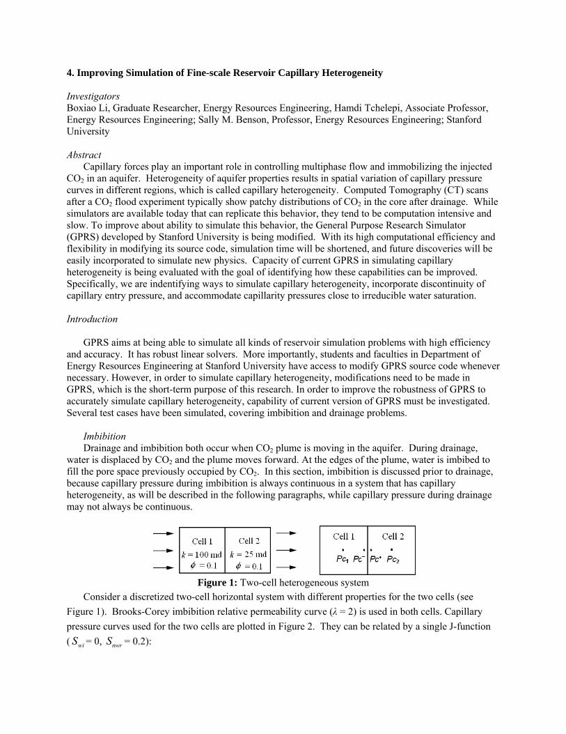
Figure 1: Two-cell heterogeneous system

Consider a discretized two-cell horizontal system with different properties for the two cells (see Figure 1). Brooks-Corey imbibition relative permeability curve (λ = 2) is used in both cells. Capillary pressure curves used for the two cells are plotted in Figure 2. They can be related by a single J-function ( wiS = 0, nwrS = 0.2):

02468

1012

0 0. 2 0. 4 0. 6 0. 8 1Sw

Pc (

psi)

Cel l 1 ( k = 100 md)Cel l 2 ( k = 25 md)

Figure 2: Imbibition capillary pressure curves of the two-cell system

Capillary pressure should be continuous across the interface of the two materials. In other words,

cP− should be equal to cP+ in Figure 1. As is shown in Figure 2, corresponding to one capillary pressure at the interface, each side of the interface has a different saturation. Therefore, the simulator has to accommodate this phenomenon correctly in order to simulate capillary heterogeneity.

A slow water imbibition is conducted from left to right on the system in Figure 1. As plotted in

Figure 3, simulation results from GPRS indicate that the water saturation profiles of the two cells are different during imbibition, while the capillary pressure of the two cells ( Pc1 and Pc2 , see Figure 1) are identical when the system is stable. When the flow rate is slow, 1c cP P−≈ , and 2c cP P+≈ , therefore it

demonstrates that c cP P− += is accommodated in GPRS simulation. Grid refinement near the interface

clearly shows that c cP P− += is always accommodated in simulation no matter how large the flow rate is. In addition, in a system shown in Figure 1, simulations with and without grid refinement yield the same result in pressure and saturation distribution, vindicating the capacity of GPRS in achieving capillary continuity across the interface regardless of the grid size.

00.10.20.30.40.50.6

0.05 0.15 0.25 0.35 0.45PVI

Sw

Cell_1 (k = 100md)Cell_2 (k = 25

d)

05

1015202530

0.05 0.15 0.25 0.35 0.45PVI

Pc (p

si)

Cell_1 (k = 100 md)

Cell_2 (k = 25 md)

Figure 3: Sw profiles and Pc values of the two cells during imbibition

Drainage When simulating drainage processes, capillary pressure may not be continuous across the interface.

Consider a flow domain sketched in Figure 1, where CO2 is injected to displace water from left to right. Brooks-Corey drainage relative permeability curve (λ = 2) is used in both cells. Capillary pressure curves used for the two cells are plotted in Figure 4. They can be related by a single J-function ( wrS = 0.2)

Note that cell 1 has a capillary entry pressure of 1 psi, while cell 2 has 2 psi. When capillary pressure

in cell 1 is below the entry pressure of cell 2, the capillary pressure of cell 2 is undefined, as indicated by the dashed lines. At this time, CO2 is blocked outside of cell 2, because the entry pressure of cell 2 is not

Sw1 Sw2

reached. Therefore, capillary pressure is discontinuous across the interface of the two cells. Such discontinuity requires special treatment in the numerical simulator.

Figure 4: Drainage capillary pressure curves of the two-cell system

Currently, GPRS can only handle simple problems, for example, a slow CO2 drainage process in the

two-cell system sketched in Figure 1. The drainage curves in Figure 4 are used to simulate the two-cell system, and the GPRS simulation results are plotted in Figure 5. CO2 does not enter cell 2 until capillary pressure at cell 1 side of the interface reaches the entry pressure of cell 2 (2 psi). After CO2 enters cell 2, capillary pressure across the interface is continuous.

Figure 5: Sw profiles and Pc values of the two cells during drainage

Progress and future work

As described in previous section, current GPRS is able to simulate basic capillary heterogeneity problems. However, improvements need to be made on GPRS in order to simulate flow in complicated domains. For example, to accurately simulate CO2 distribution in a core sample after CO2 injection, Krause, M. et al. (2009) discretized the core (8 inch in length and 2 inch in diameter) into more than 60,000 cells [4]. If each cell has a unique permeability and porosity value, there will be more than 60,000 capillary pressure curves in the simulation. How to efficiently calculate these curves and their derivatives based on a single J-function is an issue that needs to be addressed. In addition, in drainage processes, as CO2 accumulates in the pore, water saturation Sw decreases, and capillary pressure Pc increases. When Sw is approaching irreducible water saturation Swi, Pc goes to infinity, and so does its derivative. To avoid infinite values, simulator should introduce a cut off on capillary pressure curves. In a flow domain with multiple capillary pressure curves, the cut off value of each capillary pressure curve may not be equal, which may cause discontinuity near Swi. Moreover, how to treat capillary discontinuity in a complicated

0

2

4

6

8

10

12

14

0 0. 2 0. 4 0. 6 0. 8 1Sw

Pc (psi)

Cel l _1 ( k = 100 md)

Cel l _2 ( k = 25 md)

flow domain that has a large number of capillary drainage curves with different entry pressures remains an important problem.

Future work will include modifying source code of GPRS to address the three problems mentioned

above. Hysteresis of capillary pressure will be added in GPRS afterwards. After that, the gravity effects and permeability model will be investigated and incorporated into GPRS. CO2 core floods will be simulated using GPRS to accurately replicate the experimental results.

If the research is successful, GPRS will be used to carry out forward and inverse simulations of CO2

coreflood experiments. It will shorten the simulation time and improve the research efficiency in the lab. Also, it can serve a testing ground for the lab to incorporate new physics and discovery into the simulator. If the long term purpose of this research is achieved, GPRS can be used to develop up-scaling techniques for reservoir scale simulations.

References 1. Chatzis, I., Morrow N.R., and Lim H.T., Magnitude and Detained Structure of Residual Oil

Saturation, paper SPE 10681, 1983. 2. Perrin, J.-C., Krause, M.H., Kuo, C.W., Miljkovic, L., and Benson, S.M., Core Scale Experimental

Study of Relative Permeability Properties of CO2 and Brine in Reservoir Rocks, Energy Procedia, V.1(1), 3515-3522, 2009.

3. Leverett, M.C., Capillary Behavior in Porous Solids, Petroleum Transactions, AIME(142), 151-169, 1941.

4. Krause, M.H., Modeling Sub-core Scale Permeability in Sandstone for Use in Studying Multiphase Flow of CO2 and Brine in Core Flooding Experiments, MS thesis, Stanford University, CA, 2009.

Contacts

Boxiao Li: [email protected]

5. Optimization of Remediation of Possible Leakage from Geologic CO2 Storage Reservoirs into Groundwater Aquifers Ariel Esposito, Graduate Researcher, Stanford University and Sally M. Benson, Professor, Stanford University Abstract

Maintaining the long term storage of CO2 is an important requirement for a large scale geologic CO2 storage project. Nevertheless, the possibility remains that the CO2 will leak out of the formation into overlying groundwater aquifers. There are many groundwater remediation technologies available that could be applied for remediating CO2 leaks. A site specific remediation plan is also important during the site selection process and necessary before storage begins. Due to the importance of protecting drinking water resources, this study determines the optimal remediation scenario for various leakage conditions. The two objectives for remediation considered here are removing any mobile CO2 and reducing the quantity of CO2 in the reservoir. The main technique to remediate the leak is to extract the CO2 in both the gaseous and dissolved phase. Another technique analyzed is to inject water to dissolve the gaseous CO2 in the groundwater and reduce the overall aqueous concentration and immobilize CO2 by capillary trapping.

The first part of our research was to determine the processes that control the size and shape of the leakage plume in the groundwater aquifer. We used the multiphase flow simulator TOUGH2 with CO2 leakage from a point source to analyze the plume at various leakage rates. At the depth of most groundwater aquifers the pressure is shallow enough that a significant portion of the CO2 is in gas phase. Due to the large difference between the density of the groundwater and the CO2, we found that the leakage rate and the quantity of CO2 have a very important impact on the resultant leakage plume. The second step was to determine the physical processes that expedite or hinder removal of the CO2 plume. Important processes include capillary trapping as a result of hysteresis in the relative permeability and capillary pressure curves, dissolution, and buoyancy induced flow. We compared the effectiveness of using vertical and horizontal extraction wells to remove the CO2. We next examined the processes that occurred during the second remediation technique where we inject water to dissolve the gaseous CO2 and reduce the overall concentration and increase capillary trapping. With an injection well, the main controlling factor on the dissolution of CO2 was the residual gas saturation and the injection well flow rate. Based on the initial simulations, the characteristics to optimize are the extraction well depth for vertical or horizontal wells, the extraction well rate, and the injection well rate. Determining the optimal remediation scheme provides a starting point for planning groundwater remediation scenarios for possible leakage events at geologic storage sites. Introduction

There are some key aspects of CO2 that are relevant to understanding the challenges of remediation. CO2 is less dense than water and due to buoyancy forces will migrate upwards until it reaches a geologic barrier. Also, once the CO2 dissolves in the formation water it forms carbonic acid which reduces the pH of the groundwater, and could lead to increased levels of trace metals such as arsenic and lead (Wang & Jaffe 2004). A decrease in pH can be accompanied by an increase in, trace metal concentrations in the groundwater from the desorption of metals from ion exchange sites found on mineral surfaces and the dissolution of the minerals themselves (Zheng et al., 2008). CO2 induced increases in the concentration in the groundwater of trace metal such as arsenic and lead, could pose a human health risk if ingested. For this reason, during remediation it is important to reduce CO2 concentration to minimize the reduction in pH and limit the possible increases in trace metal concentrations as well as remove the CO2 from the groundwater aquifer.

Background From a review of the current research on the remediation of CO2 leaks from geologic storage

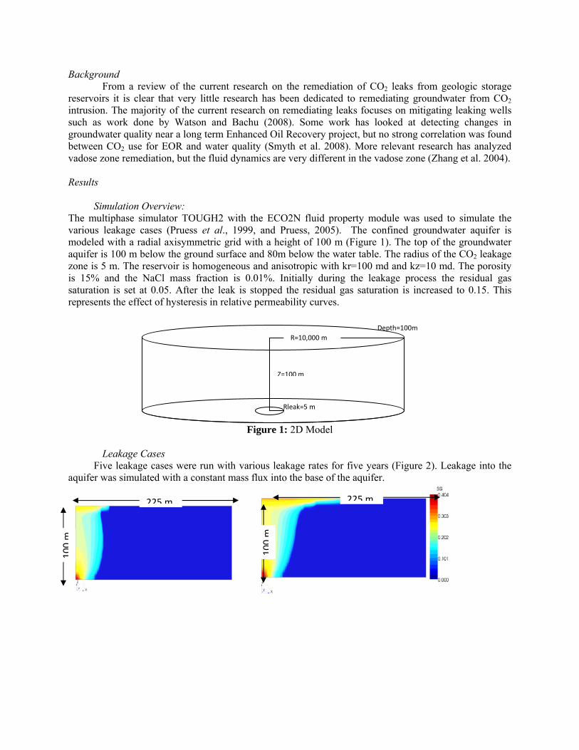
reservoirs it is clear that very little research has been dedicated to remediating groundwater from CO2 intrusion. The majority of the current research on remediating leaks focuses on mitigating leaking wells such as work done by Watson and Bachu (2008). Some work has looked at detecting changes in groundwater quality near a long term Enhanced Oil Recovery project, but no strong correlation was found between CO2 use for EOR and water quality (Smyth et al. 2008). More relevant research has analyzed vadose zone remediation, but the fluid dynamics are very different in the vadose zone (Zhang et al. 2004). Results Simulation Overview: The multiphase simulator TOUGH2 with the ECO2N fluid property module was used to simulate the various leakage cases (Pruess et al., 1999, and Pruess, 2005). The confined groundwater aquifer is modeled with a radial axisymmetric grid with a height of 100 m (Figure 1). The top of the groundwater aquifer is 100 m below the ground surface and 80m below the water table. The radius of the CO2 leakage zone is 5 m. The reservoir is homogeneous and anisotropic with kr=100 md and kz=10 md. The porosity is 15% and the NaCl mass fraction is 0.01%. Initially during the leakage process the residual gas saturation is set at 0.05. After the leak is stopped the residual gas saturation is increased to 0.15. This represents the effect of hysteresis in relative permeability curves.

Figure 1: 2D Model

Leakage Cases

Five leakage cases were run with various leakage rates for five years (Figure 2). Leakage into the aquifer was simulated with a constant mass flux into the base of the aquifer.

R=10,000 mDepth=100m

Z=100 m

Rleak=5 m

100m

225 m

100m

225 m

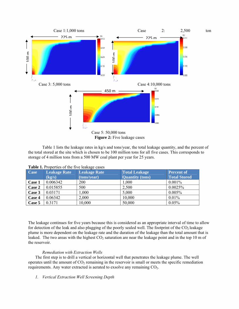
Case 1:1,000 tons Case 2: 2,500 ton

Case 3: 5,000 tons Case 4:10,000 tons

Case 5: 50,000 tons

Figure 2: Five leakage cases

Table 1 lists the leakage rates in kg/s and tons/year, the total leakage quantity, and the percent of the total stored at the site which is chosen to be 100 million tons for all five cases. This corresponds to storage of 4 million tons from a 500 MW coal plant per year for 25 years. Table 1. Properties of the five leakage cases Case Leakage Rate

(kg/s) Leakage Rate (tons/year)

Total Leakage Quantity (tons)

Percent of Total Stored

Case 1 0.006342 200 1,000 0.001% Case 2 0.015855 500 2,500 0.0025% Case 3 0.03171 1,000 5,000 0.005% Case 4 0.06342 2,000 10,000 0.01% Case 5 0.3171 10,000 50,000 0.05% The leakage continues for five years because this is considered as an appropriate interval of time to allow for detection of the leak and also plugging of the poorly sealed well. The footprint of the CO2 leakage plume is more dependent on the leakage rate and the duration of the leakage than the total amount that is leaked. The two areas with the highest CO2 saturation are near the leakage point and in the top 10 m of the reservoir.

Remediation with Extraction Wells The first step is to drill a vertical or horizontal well that penetrates the leakage plume. The well

operates until the amount of CO2 remaining in the reservoir is small or meets the specific remediation requirements. Any water extracted is aerated to exsolve any remaining CO2.

1. Vertical Extraction Well Screening Depth

100m

450 m

100m

225 m

100m

225 m

The extraction well is placed at the center of the leakage plume. The extraction well is operated with a constant pressure constraint at the top of the well in terms of meters of hydraulic head which ranged from 5 m to 50 m. For Case 1 screening the well from z=10m to z=100m leads to an effective extraction scenario because the CO2 is being consistently removed along the depth of the reservoir. The progression of the remediation at two years is shown in Figure 3 for a hydraulic head of 5 m and the dashed line shows the original plume.

Figure 3: Case 1: Extraction well screened from z=10 m to z=100 m at 2 years

Any water flowing into the well will avoid areas with high gas saturation observed in the larger

flow rate cases and can lead to inefficient remediation. An alternative approach is to extract first from the areas with high gas saturation to reduce differences in the saturation along the depth of the aquifer. Once a consistent saturation distribution is reached, begin extraction with a well screened the entire depth of the aquifer. Based on this alternative approach, the following three step well screening process was analyzed for Case 3. The first extraction step utilized a well screened from z=40 m to z=90 m with extraction with 20 m of hydraulic head (0.296 MPa) at z=90 m for three years (Figure 4).

Figure 4: Case 3: Extraction well screened from z=40 m to z=90 m after 3 yrs

To remove the gas remaining at the top of the aquifer, the packers are placed at z=95 m and z=100 m to isolate the top section. The well is operated for 325 days until most of the gas is removed. Figure 5 depicts the leakage plume at 160 days and at 325 days.

Figure 5. Case 3: Extraction well from z=95 m to z=100 m for 160 days and 325 days

100

225 m10

0 m

225 m

100 m

225 m

100 m

225 m

Now the reservoir is at consistent gas saturation close to 15%. The final stage is screening the well the

entire depth of the aquifer. During this third phase the extraction of the CO2 is very slow with approximately 240 tons removed per year resulting in an additional 17 years before all the CO2 is removed and a total time of 21 years. This remediation time frame is too long and other options need to be considered.

2. CO2 Extraction Using Horizontal Wells From the previous analysis it is clear that CO2 is difficult to efficiently extract with vertical wells. To

overcome this difficulty, we examine the potential of horizontal wells for removing the CO2. For this simulation the 3D grid shown in Figure 6 is used with a z=100 m, y= 2000 m, and x=3000 m. The CO2 leaks into a square grid block that is 5 m wide at the base of the reservoir which is located at x=1000 m and y=1000 m.

Figure 6. 3D Model

The resulting leakage plume for Case 3 looks slightly different from the 2D case even though the

leakage rate is the same (Figure 7). The main difference is that less accumulation has occurred at the top of the reservoir.

Figure 7. Case 3- 3D: Leakage Plume

With a horizontal extraction well the depth of the well is an important criterion to optimize. To

reduce the mobile gas phase the horizontal extraction well needs to be placed close enough to the secondary plume of CO2 at the top of the reservoir. As shown in Figure 8, a horizontal well placed at z=50 m does not capture much of the accumulated CO2 at the top. However, this extraction well removes 620 tons of CO2 per year during the first five years which is a significant improvement over the vertical extraction well. A horizontal extraction well placed at z=90m was effective at reducing the mobile CO2 at the top of the aquifer.

2000

3000 m

100 m

250 m

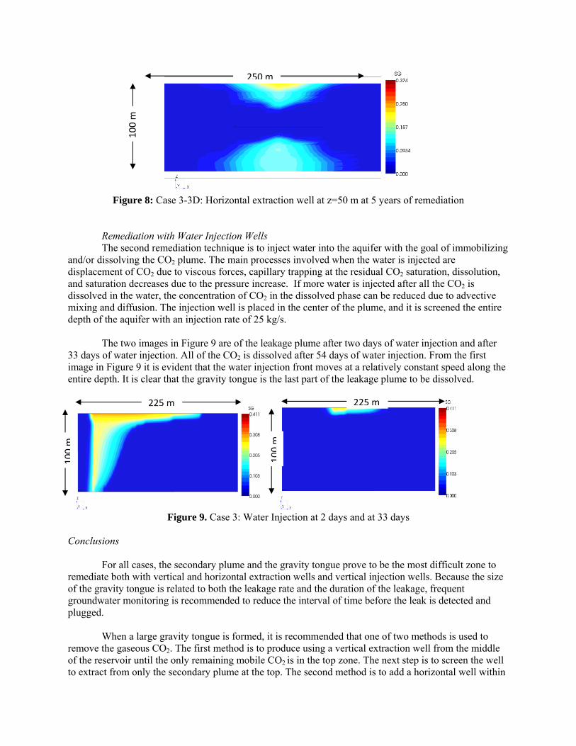
Figure 8: Case 3-3D: Horizontal extraction well at z=50 m at 5 years of remediation

Remediation with Water Injection Wells The second remediation technique is to inject water into the aquifer with the goal of immobilizing

and/or dissolving the CO2 plume. The main processes involved when the water is injected are displacement of CO2 due to viscous forces, capillary trapping at the residual CO2 saturation, dissolution, and saturation decreases due to the pressure increase. If more water is injected after all the CO2 is dissolved in the water, the concentration of CO2 in the dissolved phase can be reduced due to advective mixing and diffusion. The injection well is placed in the center of the plume, and it is screened the entire depth of the aquifer with an injection rate of 25 kg/s.

The two images in Figure 9 are of the leakage plume after two days of water injection and after 33 days of water injection. All of the CO2 is dissolved after 54 days of water injection. From the first image in Figure 9 it is evident that the water injection front moves at a relatively constant speed along the entire depth. It is clear that the gravity tongue is the last part of the leakage plume to be dissolved.

Figure 9. Case 3: Water Injection at 2 days and at 33 days

Conclusions

For all cases, the secondary plume and the gravity tongue prove to be the most difficult zone to remediate both with vertical and horizontal extraction wells and vertical injection wells. Because the size of the gravity tongue is related to both the leakage rate and the duration of the leakage, frequent groundwater monitoring is recommended to reduce the interval of time before the leak is detected and plugged.

When a large gravity tongue is formed, it is recommended that one of two methods is used to

remove the gaseous CO2. The first method is to produce using a vertical extraction well from the middle of the reservoir until the only remaining mobile CO2 is in the top zone. The next step is to screen the well to extract from only the secondary plume at the top. The second method is to add a horizontal well within

100 m

250 m10

0m

225 m

100m

225 m

the top 10 m of the reservoir to extract the gaseous CO2 from the top. Injection of water is an effective measure to quickly immobilize all the CO2 and reduce overall CO2 concentration. To reduce the quantity of CO2 in the reservoir, vertical wells perform effectively for the low leakage rate for Case 1. For the larger leakage rate cases, a horizontal well placed halfway through the reservoir is highly recommended to speed the removal of the CO2.

The remediation of CO2 leakage into a groundwater aquifer is a challenging activity that will vary for each leakage event based on the leakage characteristics and groundwater aquifer properties. For this reason, a remediation plan is necessary before the geologic carbon storage project begins. A remediation plan may also improve the public perception of carbon capture and storage (CCS) and ease site selection and approval. Large unmitigated releases of CO2 from a geologic storage site into groundwater aquifers may significantly hinder the widespread use of CCS as a carbon mitigation technique. Publications Esposito, A., S.M. Benson “Remediation of Possible Leakage from Geologic CO2 Reservoirs into

Groundwater Aquifers.” NETL: 8th Annual Conference on Carbon Capture & Sequestration. Pittsburgh, PA May 4-7, 2009 (Poster)

A. Esposito and S.M. Benson, 2010. Optimization of Remediation of Possible Leakage from Geologic CO2 Storage Reservoirs into Groundwater Aquifers, SPE-133604, Western North America Regional Meeting held in Anaheim, California, USA, 26–30 May 2010.

References 1. S. M. Benson and M. Celia, P. Cook., B. Gunter, J. Ennis King, E. Lindegerg, S. Lombardi et al.2005.

Underground Geological Storage, IPCC Special Report on Carbon Dioxide Capture and Storage, Chapter 5. Cambridge University Press, Cambridge, U.K.

2. Pruess, K. 2005. ECO2N: A TOUGH2 Fluid Property Module for Mixtures of Water, NaCl and CO2. Berkeley, California: Lawrence Berkeley National Labs Report LBNL-57952, Earth Science Division, University of California, Berkeley

3. Pruess, K., Oldenburg, C., and Moridis, G. 1999. TOUGH2 User’s Guide Version 2.0. Berkeley, California: Lawrence Berkeley National Labs Report LBNL-43134, Earth Science Division, University of California, Berkeley

4.Smyth, R. and S. Hovorka, J. Lu, K. Romanak, J.W. Partin, C. Wong. 2008. Assessing risk to fresh water resources from long term CO2 injection laboratory and field studies. Greenhouse Gas Technology Conference-9, Washington D.C. , USA.

5.Wang S., and P. R. Jaffe. 2004. Dissolution of a mineral phase in potable aquifers due to CO2 releases from deep formations; effect of dissolution kinetics. Energy Conversion and Management 45

6.Watson, T. and S. Bachu .2008. Identification of Wells With High CO2-Leakage Potential in Mature Oil Fields Developed for CO2-Enhanced Oil Recovery. SPE/DOE Improved Oil Recovery Symposium, Tulsa, Oklahoma, USA.

7. Zhang, Y., and C. Oldenburg, S.M. Benson. 2004. Vadose zone remediation of carbon dioxide leakage from geologic carbon dioxide sequestration sites. Vadose Zone Journal 3(3): 858-866.

8. Zheng, L., J. Apps, Y. Zhang, T. Xu, & J. Birkholzer 2009, Reactive Transport Simulations to Study Groundwater Quality Changes in Response to CO2 leakage from Deep Geological Storage Energy Procedia 1(1): 1887-1894.

Contacts Ariel Esposito: [email protected] Sally M. Benson: [email protected]


5. Using Stable Isotopes of Carbon in the Surface Monitoring for CO2 Leakage Over Carbon Sequestration Sites Investigators Samuel Krevor, Postdoctoral Researcher, Jean-Christophe Perrin, Postdoctoral Researcher, Ariel Esposito, Graduate Researcher, Energy Resources Engineering, Stanford University, Chris Rella, Picarro and Sally M. Benson Abstract

Carbon isotopes of CO2 provide an opportunity to distinguish between natural biogenic CO2 fluxes from the ground and CO2 leaking from a sequestration reservoir. Rapid measurements of the 13CO2 composition of CO2 in gas samples in the field is now possible through the use of wavelength scanned cavity ringdown spectroscopy (WSCRDS). In an initial proof of concept of the use of stable isotope measurements for the detection of a low-level CO2 leak, a portable WSCRDS has been used to detect, locate, and characterize an intentional leakage of CO2 from an underground pipeline at the ZERT experimental facility in Bozeman, Montana. Rapid (1 hour) walking surveys of the 100-meter by 100-meter site surrounding the pipeline were collected. The resulting concentration and 13C isotopic abundance maps were analyzed using Keeling plots, permitting not only the identification of specific leakage locations, but providing the ability to distinguish petrogenic sources of CO2 from biogenic sources. The ability to rapidly and reliably detect 12CO2 and 13CO2 concentration anomalies and identify the isotopic composition of the source flux provides a powerful and practical tool for detecting leakage from CO2 sequestration projects. Work continues on the development of this technique for use on the large spatial scales likely relevant for industrial CO2 sequestration projects, to understand the limits of the use of stable isotopes in the detection and characterization of CO2 surface leakage, and in techniques for the quantification of leak flux rates. Introduction Effective monitoring for geologic sequestration sites will be essential for the commercial-scale deployment of carbon sequestration. Desirable qualities of practical monitoring technologies include low costs, rapid deployment over large spatial scales, high resolution, reliability, and positive identification of a leak should it exist. Unlike many of the approaches that are currently used to monitor sequestration projects, near-surface monitoring technologies offer the opportunity to directly detect and quantify leakage into the atmosphere (Benson 2005). Near-surface detection and quantification can be made complicated, however, due to large temporal and spatial variations in natural background CO2 fluxes from biological processes (Benson 2006, Lewicki 2005). Carbon isotopes provide an opportunity to distinguish between natural biogenic CO2 fluxes from the ground and CO2 leaking from a sequestration reservoir that has ultimate origins in a process giving it a distinct isotopic signature such as natural gas processing. Until recently, measuring isotopic compositions of gases was a time-consuming and expensive process utilizing mass-spectrometry, not practical for deployment in a high-resolution survey of a potential leakage site at the surface (Michener 2007). Recent developments in commercially available instruments utilizing wavelength scanned cavity ringdown spectroscopy (WS-CRDS) and Fourier transform infrared spectroscopy (FT-IR) have made it possible to rapidly measure the isotopic composition of gases including the 13C and 12C isotopic composition of CO2 in a field setting (Steele 2008, Esler 2000).

The focus of this research is to develop methods for utilizing the rapid and mobile measurement of the isotopic composition of gas samples for the surface monitoring of CO2 over sequestration sites. In an initial proof of concept, we have used a commercially available WS-CRDS to observe an intentional leakage of CO2 at an experimental facility built by the Zero Emissions Research Technology Project

(ZERT) lead by Montana State University (Spangler 2009). Surveys were performed such that spatially varying maps could be constructed of the 13C isotopic signature of the ground-source CO2. The goal was to see if a leak could be detected and the source characterized through an observation of the isotopic signature of the source gas alone. Background There are many capabilities by which surface monitoring technologies need to be evaluated. A monitoring program may include technologies to be used for detecting leaks or confirming the absence of leaks over a particular spatial domain, identifying the source of a leak, and quantifying the leak rate. Many technologies have been developed in the occupational hazard industry as well as for ecology that could potentially be deployed for the purpose of surface monitoring over sequestration sites. Handheld monitors using infrared sensing technology can readily determine CO2 concentrations. Eddy flux covariance towers have been developed to calculate the net gas flux into the surface layer from the ground and may be useful in leak detection. Various groups are exploring the potential to spike injected CO2 with radioisotopes or rare noble gases so that once a leak was detected, an identification of the source could be established.

The spatial and temporal scales for which these technologies have been developed, however, leave important gaps in the needs for CCS monitoring. Low-level leak detection over large spatial scales in particular is an area for which no currently proposed technologies or methods exist (Benson 2005, 2006).

Experimental Methods At the site an approximately 100-meter horizontal well has been drilled below an alfalfa field with a

depth varying between 1-3 meters below the surface. The well has perforations in six zones separated by packers along the central 70 meters of the well. For 30 days starting July 15, 2009, CO2 was injected at a rate of 0.2 tonnes per day, with equal amounts of CO2 reaching each of the six zones along the pipeline. The injection rate is designed to simulate a hypothetical leakage from a commercial scale sequestration project at an annual rate of between .001 and .01%. The CO2 from the tanks has a d13C = -52‰ with d13C representing the ‰ deviation of the 13C: 12C ratio in the CO2 relative to the ratio in an international standard,Vienna Pee Dee Belemnite (VPDB) (Michener 2007). This is typical of CO2 sourced from natural gas processing facilities and is far more negative d13C signature than either atmospheric CO2 (approx. -8‰) or CO2 from soil respiration (approx. -26‰) at the site.

The CO2 isotopic composition and concentration measurements were taken with a Picarro WS-CRDS analyzer, a low-drift, high precision greenhouse gas analyzer (Crosson 2008). In WS-CRDS, a gas sample is introduced into a high-finesse optical cavity, and the absorbance of the sample is determined, thus providing concentration or isotopic ratio measurements of particular gas species of interest. The Picarro instrument precisely controls the temperature and pressure of the sample within the optical cavity to within a few hundredths of a degree Kelvin and .05 Torr over a large range of ambient pressures and temperatures. In addition, it is unaffected by a wide range in humidity and holds calibration for more than 30 days (Crosson 2008). The instrument was calibrated for the measurement of 12CO2 and 13CO2 at a precision of 200 ppbv and 15 ppbv respectively. For the gas inlet, 1/8-inch diameter tubing was connected to the instrument-sampling inlet. The flow-rate of gas was set to approximately 150 ml/min, equivalent to a gas residence time of 4 seconds in the optical cavity. Simultaneous with CO2 concentrations (including 13C), position data was logged using a Trimble ProXT GPS receiver. Datapoints are taken approximately every second. The instrument itself is contained within dimensions of 24" long, 17" wide and 10" tall, weighs approximately 60 lbs, has been designed to withstand substantial shock, and is thus suitable for use in a field setting. To create a mobile platform, the analyzer was powered using batteries and housed in a small cart.

The surveys consisted of traverses of the site at a walking speed of 1-2m/sec (equivalent to 40-85 km over 12 hours) along the length of the pipeline and extending out 50 meters on either side of the pipeline with the end of the gas inlet tube approximately 9 centimeters above the ground. Some locations were inaccessible due to the presence of sensitive equipment in the ground at the site. The surveys were performed both during the day and during the evening when CO2 flux due to respiration from the soil is markedly different.

The Keeling plot is used to identify the isotopic signature of a source flux of CO2 entering an ambient or background atmosphere with a constant CO2 concentration (Cb) and d13C signature (d13C b) (Keeling 1961, Pataki 2003). Using simple mass balances, one may derive an equation for the measured d13C (d13C a) as a linear function with a slope equal to the inverse of the total measured CO2 concentration (Ca) and vertical intercept the d13C of the source flux (d13Cs). i.e. equation 1. In this study, we seek to identify the isotopic signature of the ground sourced CO2, which takes the place of d13Cs in equation 1, as it moves into the local atmosphere, the background atmosphere in equation 1. By plotting the measured isotopic composition (d13Ca) of gas samples measured above the ground against the inverse of measured values of total CO2 concentration (Ca) in those samples, we identify the d13Cs of gas as the intercept of the least squares regression based best-fit line.

δ13ca = cb (δ13cb −δ13cs)

1ca

+ δ13cs (1)

At the ZERT experimental field site, the natural ground sourced CO2 has a d13C = -26‰ (Spangler 2009). In locations where CO2 was seeping from the underground pipeline, we could expect that the isotopic signature of the ground source CO2 would be altered due to the contribution from the injected CO2, isotopically depleted relative to the natural ground source (d13C = -52‰). This could be used to precisely identify locations of the leakage. To this end, we selected data within 10-meter by 10-meter sub-blocks of the measured area, made Keeling plots, and constructed a spatially varying d13Cs map of the area. Data points were generated at a 1-meter resolution and interpolated using triangle-based linear interpolation. Locations were omitted from the interpolation and map if there were less than 20 data points within the 10 meter by 10 meter area. The WS-CRDS does not measure 12CO2 and 13CO2 concentrations simultaneously. Thus, some error is introduced in calculating the d13C if the CO2 concentration is changing rapidly. Before Keeling plots were constructed, data was filtered to remove points taken during times when the total CO2 concentration was varying more than 10 ppm/s.

Results

Keeling Plot Identification of the ground flux CO2 Constructing the Keeling plot for data collected across the site, we identified the d13Cs of gas

measured at locations away from (>10 m) the pipeline to have a value of -20‰, typical of biogenic CO2 (figure 1(a)). Including locations above the pipeline (within 10 m), the Keeling plot identified d13C$ value lowers to -41‰, representative of the injected gas (figure 1(b)).

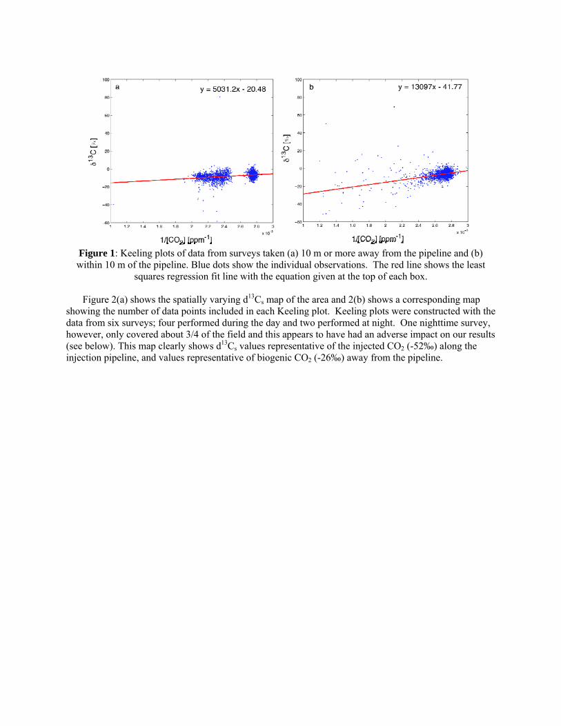
Figure 1: Keeling plots of data from surveys taken (a) 10 m or more away from the pipeline and (b) within 10 m of the pipeline. Blue dots show the individual observations. The red line shows the least

squares regression fit line with the equation given at the top of each box.

Figure 2(a) shows the spatially varying d13Cs map of the area and 2(b) shows a corresponding map showing the number of data points included in each Keeling plot. Keeling plots were constructed with the data from six surveys; four performed during the day and two performed at night. One nighttime survey, however, only covered about 3/4 of the field and this appears to have had an adverse impact on our results (see below). This map clearly shows d13Cs values representative of the injected CO2 (-52‰) along the injection pipeline, and values representative of biogenic CO2 (-26‰) away from the pipeline.

Figure 2: (a) Spatially-varying d13Cs values for ground source CO2 ([‰]) and (b) map showing the number of points used to make each Keeling plot ([number of points]). The plot was made utilizing Keeling plots of measured data within 10 meter by 10 meter areas around each plot location. Blank areas are locations where there were less than 20 datapoints with which to create the Keeling plots. Black line shows the path of the pipeline.

Conclusions It is clear that leak identification is possible through the observation of the isotopic composition of the

ground sourced CO2. This is particularly useful when natural or anthropogenic background fluxes are too high or too variable to detect leakage from concentration measurements alone, or as identification tool to positively identify a CO2 source based on its distinct isotopic signatures. Moving at a speed of 1 m/s in 5 meter wide traverses of the 100 meter by 100 meter area, there were generally enough data points (e.g. 20 at low concentrations and 20 at high concentrations) within a 10 m by 10 m area to construct Keeling plots utilizing data from effectively two daytime surveys and two night time surveys. Thus the values in figure 2 are constructed from datapoints taken within an approximately 5-meter radius from the given value.

Samples collected from a mobile platform, such as an ATV or other automobile, moving at a rate of 1-2 m/s with a sampling frequency of 1 per second provide coverage of 40 to 85 km/day and 43,200 sample points/day. A CO2 plume from a mature commercial scale project may extend over an area of 100 km2. With the data sampling and acquisition parameters used here, it would be possible to monitor the entire area (1,000 km of sampling traverse within a 100 km2 area) with a two to four week survey. In areas where anomalous 12CO2 and 13CO2 concentrations are detected, higher resolutions surveys could be used to precisely locate the extent of the leak and characterize the isotopic composition of the source more carefully.

Publications S. Krevor, J.C. Perrin, A. Esposito, C. Rella, and S. Benson. “Rapid Detection and Characterization of Surface CO2 Leakage Through the Realtime Measurement of d13C Signatures in CO2 Flux from the Ground.” International Journal of Greenhouse Gas Control (Accepted, 2010). Presentations 1. S. Krevor, J.C. Perrin, A. Esposito, C. Rella, and S. Benson Rapid Detection and Characterization of

Surface CO2 Leakage Through the Realtime Measurement of d13C Signatures in CO2 Flux from the Ground. Oral Presentation. American Geophysical Union Fall Meeting 2009, San Francisco, CA

2. S. Krevor, J.C. Perrin, A. Esposito, C. Rella, and S. Benson Rapid Detection and Characterization of Surface CO2 Leakage Through the Realtime Measurement of d13C Signatures in CO2 Flux from the Ground. Oral Presentation. European Geoscienes Union Meeting 2010, Vienna, Austria

3. S. Krevor, J.C. Perrin, A. Esposito, C. Rella, and S. Benson Rapid Detection and Characterization of Surface CO2 Leakage Through the Realtime Measurement of d13C Signatures in CO2 Flux from the Ground. Oral Presentation. 9th Annual Conference on Carbon Capture and Sequestration May 2010, Pittsburgh PA

4. S. Krevor, J.C. Perrin, A. Esposito, C. Rella, and S. Benson Rapid Detection and Characterization of Surface CO2 Leakage Through the Realtime Measurement of d13C Signatures in CO2 Flux from the Ground. Oral Presentation. Goldschmidt, Knoxville, Tennessee, June 2010

References S. M. Benson and M. Celia, P. Cook., B. Gunter, J. Ennis King, E. Lindegerg, S. Lombardi et al.2005.

Underground Geological Storage, IPCC Special Report on Carbon Dioxide Capture and Storage, Chapter 5. Cambridge University Press, Cambridge, U.K.

E.R. Crosson. A cavity ring-down analyzer for measuring atmospheric levels of methane, carbon dioxide, and water vapor. Applied Physics B, 92:403-408, 2008.

M.B. Esler, D.W.T. Gri_th, S.R. Wilson, and L.P. Steele. Precision trace gas analysis by ft-ir spectroscopy. 2. the 13c/12c isotope ratio of co2. Analytical Chemistry, 72:216-221, 2000.

Keeling, C. D., 1961. The concentration and isotopic abundances of carbon dioxide in rural and marine

air. Geochimica et Cosmochimica Acta 24, 277{298. Lewicki, J., Hilley, G., Oldenburg, C., 2005. An improved strategy to detect co2 leakage for veri_cation

of geologic carbon sequestration. Geophysical Research Letters 32 (L19403) Michener, R., Lajtha, K. (Eds.), 2007. Stable Isotopes in Ecology and Environmental Science, second

edition Edition. Blackwell Publishing. Pataki, D., Ehleringer, J., Flanagan, L., Yakir, D., Bowling, D., Still, C., 2003. The application and

interpretation of keeling plots in terrestrial carbon cycle research. Global Biogeochemical Cycles. Spangler, L. H., Dobeck, L. M., Repasky, K., Nehrir, A., Humphries, S., Barr, J., Keith, C., Shaw, J.,

Rouse, J., Cunningham, A., Benson, S., Oldenburg, C. M., Lewicki, J. L., Wells, A., Diehl, R., Strazisar, B., Fessenden, J., Rahm, T., Amonette, J., Barr, J., Pickles, W., Jacobson, J., Silver, E., Male, E., Rauch, H., Gullickson, K., Trautz, R., Kharaka, Y., Birkholzer, J., Wielopolski, L., 2009. A controlled field pilot for testing near surface CO2 detection techniques and transport models. Energy Procedia 1 (2143-2150).

Steele, L., Loh, Z., Etheridge, D., Krummel, P., van Pelt, A., 2008. Continuous greenhouse gas and isotopic carbon dioxide measurements via ws-crds analyzers: Investigations in real-time monitoring at CO2 geological storage sites. In: American Geophysical Union Fall Meeting.

Contacts Sally Benson: [email protected] Sam Krevor: [email protected]

Publications

A. Esposito and S.M. Benson, 2010. Optimization of Remediation of Possible Leakage from Geologic CO2 Storage Reservoirs into Groundwater Aquifers, SPE-133604, Western North America Regional Meeting held in Anaheim, California, USA, 26–30 May 2010.

Krause, M., Perrin, J-C., and Benson, S. M., 2009. Modeling Permeability Distributions in a Sandstone Core for History Matching Coreflood Experiments. Proc. SPE International Conference on CO2 Capture, Storage and Utilization. San Diego, CA USA, 2-4 November. Also, submitted for Publication in SPEJ.

S. Krevor, J.C. Perrin, A. Esposito, C. Rella, and S. Benson Rapid Detection and Characterization of Surface CO2 Leakage Through the Realtime Measurement of d13C Signatures in CO2 Flux from the Ground. Accepted. 2010 International Journal of Greenhouse Gas Control.

C-W Kuo, J-C Perrin, and S M. Benson, 2010. Effect of Gravity, Flow Rate, and Small Scale Heterogeneity on Multiphase Flow of CO2 and Brine, SPE 132607, Western North America Regional Meeting held in Anaheim, California, USA, 26–30 May 2010.

Residual Trapping of Carbon Dioxide - Stanford University

Documents

Transcript of Residual Trapping of Carbon Dioxide - Stanford University