Residential mortgage loan securitization and the subprime ...

Residential mortgage loan securitization and the subprime crisis

S. Thomas, M.Sc

Thesis submitted in partial fulfilment of the requirements for the degree

Philosophiae Doctor in Applied Mathematics at the Potchefstroom Campus of

the North West University (NWU-PC)

PROTECTION

SELLER

Monoline Insurer

Monoline

Guarantee

Monoline

Premiums

Credit

Rating

Agency

PROTECTION BUYER

Subprime

Investing Bank

SUBPRIME

DEALER BANK

Special

Purpose Vehicle

SMP Bond

Purchase

SMP Bond

Principal & Interest

Figure: Structured Mortgage Products Wrapped by Monoline Insurance

Supervisor: Prof. Mark A. Petersen

Co-Supervisor: Dr. Janine Mukuddem-Petersen

November 2010 Potchefstroom

Acknowledgments

Firstly, I thank the Almighty for His grace in enabling me to complete this thesis.

I would like to express my gratitude towards my supervisor Prof. Mark A. Petersen, of

the Mathematics and Applied Mathematics Department at NWU-PC, for his splendid

guidance, suggestions, explanations and motivation as well as co-supervisor, Dr. Janine

Mukuddem-Petersen, for the guidance provided during the completion of this thesis.

Also I wish to thank Drs. Thahir Bosch, Hennie Fouche, Frednard Gideon, Mmboniseni

Mulaudzi, Ilse Schoeman, and Aaron Tau as well as Charlotte Senosi, Bernadine de

Waal, Candice de Ponte, Dingaan Khoza and Sarah Mokoena from the Modeling in

Finance, Risk and Banking (MFRB) Research Group at the North-West University for

contributing to the various debates about subprime mortgage origination, securitization,

risk, data and bailouts from 2008 onwards.

I acknowledge the emotional support provided by my family; daughter Rose, husband

Rex and my parents Thomas and Valsamma.

A special thanks to George K John (Gejo) for introducing me to my supervisor.

Furthermore, I am grateful to the National Research Foundation (NRF) for providing

me with funding during the duration of my studies. Finally I would like to thank

the Business Mathematics and Informatics Research Unit in the School of Computer,

Mathematical and Statistical Sciences at NWU-PC for the financial support received.

Page i of 179

Preface

One of the contributions made by the NWU-PC to the activities of the stochastic analysis com-

munity has been the establishment of an active research group MFRB that has an interest in

institutional finance. In particular, MFRB has made contributions about modeling, optimization,

regulation and risk management in insurance and banking. Students who have participated in

projects in this programme under Prof. Petersen’s supervision are listed below.

Level Student Graduation Title

MSc T Bosch May 2003 Controllability of HJMM

Cum Laude Interest Rate Models

MSc CH Fouche May 2006 Continuous-Time Stochastic

Cum Laude Modelling of Capital Adequacy

Ratios for Banks

MSc MP Mulaudzi May 2008 A Decision Making Problem

Cum Laude in the Banking Industry

PhD CH Fouche May 2008 Dynamic Modeling

of Banking Activities

PhD F Gideon Sept. 2008 Optimal Provisioning for Deposit

Withdrawals and Loan Losses

in the Banking Industry

MSc MC Senosi May 2009 Discrete Dynamics of Bank

S2A3 Winner Credit and Capital and

for NWU-PC their Cyclicality

PhD T Bosch May 2009 Management and Auditing of

Bank Assets and Capital

PhD BA Tau May 2009 Bank Loan Pricing and

Profitability and Their

Connections with Basel II and

the Subprime Mortgage Crisis

PhD MP Mulaudzi May 2010 The Subprime Mortgage Crisis:

Asset Securitization & Interbank Lending

MSc B De Waal May 2011 Stochastic Optimization of Subprime Residential

Cum Laude Mortgage Loan Funding and its Risks

PhD MC Senosi May 2011 Discrete-Time Modeling of Subprime Mortgage Credit

PhD S Thomas May 2011 Residential Mortgage Loan Securitization

and The Subprime Crisis

Postdoc J Mukuddem-Petersen 2006-9 Finance, Risk and Banking

Postdoc T Bosch 2010 Finance, Risk and Banking

Page ii of 179

Declaration

I declare that, apart from the assistance acknowledged, the research presented in this thesis is

my own unaided work. It is being submitted in partial fulfilment of the requirements for the

degree Philosophiae Doctor in Applied Mathematics at the Potchefstroom Campus of the North

West University. It has not been submitted before for any degree or examination to any other

University.

Nobody, including Prof. Mark A. Petersen, but myself is responsible for the final version of this

thesis.

Signature.................................

Date......................................

Page iii of 179

Executive Summary

Many analysts believe that problems in the U.S. housing market initiated the 2008-2010 global

financial crisis. In this regard, the subprime mortgage crisis (SMC) shook the foundations of the

financial industry by causing the failure of many iconic Wall Street investment banks and promi-

nent depository institutions. This crisis stymied credit extension to households and businesses

thus creating credit crunches and, ultimately, a global recession. This thesis specifically discusses

the SMC and its components, causes, consequences and cures in relation to subprime mortgages,

securitization, as well as data. In particular, the SMC has highlighted the fact that risk, credit rat-

ings, profit and valuation as well as capital regulation are important banking considerations. With

regard to risk, the thesis discusses credit (including counterparty), market (including interest rate,

basis, prepayment, liquidity and price), tranching (including maturity mismatch and synthetic),

operational (including house appraisal, valuation and compensation) and systemic (including ma-

turity transformation) risks. The thesis introduces the IDIOM hypothesis that postulates that the

SMC was largely caused by the intricacy and design of subprime agents, mortgage origination and

securitization that led to information problems (loss, asymmetry and contagion), valuation opaque-

ness and ineffective risk mitigation. It also contains appropriate examples, discussions, timelines

as well as appendices about the main results on the aforementioned topics. Numerous references

point to the material not covered in the thesis, and indicate some avenues for further research.

In the thesis, the primary subprime agents that we consider are house appraisers (HAs), mortgage

brokers (MBs), mortgagors (MRs), servicers (SRs), SOR mortgage insurers (SOMIs), trustees,

underwriters, credit rating agencies (CRAs), credit enhancement providers (CEPs) and monoline

insurers (MLIs). Furthermore, the banks that we study are subprime interbank lenders (SILs),

subprime originators (SORs), subprime dealer banks (SDBs) and their special purpose vehicles

(SPVs) such as Wall Street investment banks and their special structures as well as subprime in-

vesting banks (SIBs). The main components of the SMC are MRs, the housing market, SDBs/hedge

funds/money market funds/SIBs, the economy as well as the government (G) and central banks.

Here, G either plays a regulatory or policymaking role. Most of the aforementioned agents and

banks are assumed to be risk neutral with SOR being the exception since it can be risk (and regret)

averse on occasion. The main aspects of the SMC – subprime mortgages, securitization, as well as

data – that we cover in this thesis and the chapters in which they are found are outlined below.

In Chapter 2, we discuss the dynamics of subprime SORs’ risk and profit as well as their valuation

under mortgage origination. In particular, we model subprime mortgages that are able to fully

amortize, voluntarily prepay or default and construct a discrete-time model for SOR risk and profit

incorporating costs of funds and mortgage insurance as well as mortgage losses. In addition, we

show how high loan-to-value ratios due to declining housing prices curtailed the refinancing of

subprime mortgages, while low ratios imply favorable house equity for subprime MRs.

Chapter 3 investigates the securitization of subprime mortgages into structured mortgage products

such as subprime residential mortgage-backed securities (RMBSs) and collateralized debt obliga-

tions (CDOs). In this regard, our discussions focus on information, risk and valuation as well as

the role of capital under RMBSs and RMBS CDOs. Our research supports the view that incen-

tives to monitor mortgages has been all but removed when changing from a traditional mortgage

Page iv of 179

model to a subprime mortgage model. In the latter context, we provide formulas for IB’s profit

and valuation under RMBSs and RMBS CDOs. This is illustrated via several examples. Chapter 3

also explores the relationship between mortgage securitization and capital under Basel regulation

and the SMC. This involves studying bank credit and capital under the Basel II paradigm where

risk-weights vary. Further issues dealt with are the quantity and pricing of RMBSs, RMBS CDOs

as well as capital under Basel regulation. Furthermore, we investigate subprime RMBSs and their

rates with slack and holding constraints. Also, we examine the effect of SMC-induced credit rating

shocks in future periods on subprime RMBSs and RMBS payout rates. A key problem is whether

Basel capital regulation exacerbated the SMC. Very importantly, the thesis answers this question

in the affirmative.

Chapter 4 explores issues related to subprime data. In particular, we present mortgage and secu-

ritization level data and forge connections with the results presented in Chapters 2 and 3.

The work presented in this thesis is based on 2 peer-reviewed chapters in books (see [99] and [104]),

2 peer-reviewed international journal articles (see [48] and [101]), and 2 peer-reviewed conference

proceeding papers (see [102] and [103]).

North-West University, South Africa SOBY THOMAS

Page v of 179

Key DefinitionsIn this section, we provide definitions of some of the key concepts discussed in the thesis. Unless

otherwise stated, the terms mortgage, mortgage loan and residential mortgage loan (RML) will

have the same meaning.

The discount rate is the rate at which the U.S. Federal Reserve lends to banks.

The federal funds rate is the interest rate banks charge each other for loans.

The London Interbank Offered Rate (LIBOR) is a daily reference rate based on the interest rates

at which banks borrow unsecured funds from banks in the London wholesale money market (or

interbank market). The risk premium is the return in excess of the LIBOR rate that a loan

extension is expected to yield.

Mortgage value may be characterized in several different ways. The face or nominal or par value

of a mortgage is its stated fixed value as given on the contract. By contrast, the market value of

a mortgage is its value in the housing market and may fluctuate quite considerably. Outstanding

value refers to the outstanding payments on mortgages. Mortgages current selling price or current

worth is called its present value (PV). The nett present value (NPV) is the difference between the

present value of cash inflows and the present value of cash outflows associated with a mortgage.

NPV is used in capital budgeting to analyze the profitability of originating mortgages. Fair value

is a method of determining what a troubled mortgage would be worth (its present value) if its

present owner sold it in the current market. Fair value assumes a reasonable marketing period, a

willing buyer and a willing seller. It assumes that the current selling price (its present value) would

rise or fall in relation to the asset’s future earnings potential.

An adjustable-rate mortgage (ARM) is a mortgage loan whose interest rate is adjustable during

its term. On the other hand, a fixed-rate mortgage (FRM) is a loan whose interest is fixed for the

duration of its term.

Mortgage default is a term used to describe mortgages that are not being repaid at all.

The delinquency rate includes mortgages that are at least one payment past due but does not include

mortgages somewhere in the process of foreclosure. In turn, foreclosure is the legal proceeding in

which a mortgagee, or other loanholder1, usually a lender, obtains a court ordered termination

of a mortgagor’s equitable right of redemption. Usually a lender obtains a security interest from

a borrower who mortgages or pledges an asset like a house to secure the loan. If the borrower

defaults and the lender tries to repossess the property, courts of equity can grant the owner the

right of redemption if the borrower repays the debt. When this equitable right exists, the mortgagor

cannot be sure that it can successfully repossess the property, thus the lender seeks to foreclose the

equitable right of redemption. Other mortgagors can and do use foreclosure, such as for overdue

taxes, unpaid contractors’ bills or overdue house appraiser dues or assessments. The foreclosure

process as applied to mortgages involves a bank or other secured creditor selling or repossessing a

parcel of real property (immovable property) after the owner has failed to comply with an agreement

between SOR and MR called a deed of trust. Commonly, the violation of the mortgage is a default

1In law, a lien is a form of security interest granted over an item of property to secure the payment of a debt orperformance of some other obligation. The owner of the property, who grants the lien, is referred to as the loanorand the person who has the benefit of the lien is referred to as the loanee.

Page vi of 179

in payment of a promissory note, secured by a lien on the property. When the process is complete,

SOR can sell the property and keep the proceeds to pay off its mortgage and any legal costs, and

it is typically said that ”the lender has foreclosed its mortgage or lien.” If the promissory note was

made with a recourse clause then if the sale does not bring enough to pay the existing balance of

principal and fees, the mortgagee can file a claim for a deficiency judgement.

Prepayment is the act of paying a mortgage in full before it is due to be paid. Voluntary prepay-

ment takes place when this act is voluntary, while involuntary prepayment results when this act

is involuntary as in default. Curtailment involves the cutting short or reduction of the contracted

mortgage term.

Cost of mortgages is the interest cost that a bank must pay for the use of funds to originate

mortgages.

Credit crunch is a term used to describe a sudden reduction in the general availability of loans (or

credit) or sudden increase in the cost of obtaining loans from banks (usually via raising interest

rates).

Subprime residential mortgage origination is the practice of originating mortgages to mortgagors

who do not qualify for market interest rates owing to various risk factors, such as income level,

size of the down payment made, credit history and employment status. In this regard, a subprime

mortgage is a loan that meets some of the following criteria. It is extended to a MR with a

poor credit history (for instance, with a FICO score below 620), it is originated by a SOR who

specializes in high-cost mortgages, became part of a so-called subprime reference mortgage portfolio

or is traded on a secondary market. Alternatively, the subprime mortgage is characterized by its

origination to mortgagors with prime credit characteristics (e.g., a high FICO score) but is a

subprime-only contract type, such as a 2/28 hybrid2 – a product not generally available in the

prime mortgage market. Mortgagors may find subprime mortgages to be worse than their prime

counterparts because of high interest rates or fees that originators charge. They also may charge

larger penalties for late payments or prepayments. Subprime mortgages are worse from originators’

perspective because they may be considered to be riskier compared to prime mortgages – there may

be a higher probability of default - so originators require those higher rates and fees to compensate

for additional risk. These mortgages can also be worse for all role players in the economy if this

risk does materialize.

Deadweight loss, also referred as excess burden or allocative inefficiency, is the cost created by

economy inefficiency. Causes of the deadweight loss can include taxes or subsidies. The deadweight

cost is dependent on the elasticity of supply and demand for a loan.

A banking agent is a person or firm that impacts the operation of the banking sector. A risk-averse

banking agent is one who avoids risky investments. A regret-averse agent3 reflects an aversion to

ex-post comparisons of its realized outcome with outcomes that could have been achieved had it

chosen differently.

In structured finance, a tranche is one of a number of related securities offered as part of the same

transaction. All the tranches together make up what is referred to as the deal’s capital structure or

2A 2/28 hybrid mortgage carries a fixed rate for the first two years; after that, the rate resets into an index rate[usually a six-month LIBOR] plus a margin.

3Alternatively, regret aversion reflects a disproportionate distaste for large regrets and, for a given menu of acts.Such regret aversion distorts the agent’s choice behavior relative to the behavior of an expected utility maximizer.

Page vii of 179

liability structure. They are generally paid sequentially from the most senior to most subordinate

(and generally unsecured), although certain tranches with the same security may be paid pari passu.

The more senior rated tranches generally have higher bond credit ratings (ratings) than the lower

rated tranches. For example, senior tranches may be rated AAA, AA or A, while a junior, unsecured

tranche may be rated BB. However, ratings can fluctuate after the debt is issued and even senior

tranches could be rated below investment grade (less than BBB). The deal’s indenture (its governing

legal document) usually details the payment of the tranches in a section often referred to as the

waterfall (because the moneys flow down). Tranches with a first lien on the assets of the asset pool

are referred to as ”senior tranches” and are generally safer investments. Typical investors of these

types of securities tend to be conduits, insurance companies, pension funds and other risk averse

investors. Tranches with either a second lien or no lien are often referred to as ”junior notes”.

These are more risky investments because they are not secured by specific assets. The natural

buyers of these securities tend to be hedge funds and other investors seeking higher risk/return

profiles. Tranches allow for the creation of one or more classes of securities whose rating is higher

than the average rating of the underlying collateral asset pool or to generate rated securities from a

pool of unrated assets. This is accomplished through the use of credit support specified within the

transaction structure to create securities with different risk-return profiles. The equity/first-loss

tranche absorbs initial losses, followed by the mezzanine tranches which absorb some additional

losses, again followed by more senior tranches. Thus, due to the credit support resulting from

tranching, the most senior claims are expected to be insulated - except in particularly adverse

circumstances - from default risk of the underlying asset pool through the absorption of losses by

the more junior claims.

Securitization is a structured finance process, which involves pooling and repackaging of cash-flow

producing financial assets into securities that are then sold to investors. In other words, securitiza-

tion is a structured finance process in which assets, receivables or financial instruments are acquired,

classified into pools, and offered for sale to third-party investment. The term ”securitization” is

derived from the fact that the form of financial instruments used to obtain funds from subprime

investing banks (SIBs) are securities.

Asset-backed securities are structured products whose cash flow depends on that of an underlying

asset. A special case is the residential mortgage-backed securities whose cash flows depend on

underlying mortgage repayments.

Structured mortgage product default refers to the situation where reference mortgage portfolio re-

turns do not attain the sum of sen and mezz claims.

Residential mortgage products include RMLs and products derived from them such as RMBSs,

CDOs, asset-backed commercial paper (ABCP) etc.

Credit enhancement is the loss on underlying reference mortgage portfolios (collateral) that can be

absorbed before the tranche itself absorbs any loss.

Equity is a term used to describe investment in the bank. Two types of equity are described below.

Common equity is a form of corporation equity ownership represented in the securities. It is a stock

whose dividends are based on market fluctuations. It is risky in comparison to preferred shares and

some other investment options, in that in the event of bankruptcy, common stock investors receive

their funds after preferred stockholders, bondholders, creditors, etc. On the other hand, common

Page viii of 179

shares on average perform better than preferred shares or bonds over time. Preferred equity, also

called preference equity, is typically a higher ranking stock than voting shares, and its terms are

negotiated between the bank and the regulator.

The leverage of a bank refers to its debt-to-capital reserve ratio. A bank is highly leveraged if this

ratio is high.

An economic equilibrium is a condition in which all acting economic influences are canceled by

others, resulting in a stable, balanced, or unchanging economic system.

Welfare programs are government initiatives that provide financial aid to troubled SORs and are

funded by taxpayers. Since the debt market is competitive in period 0, by assumption, SIB receives

the entire expected surplus, thus their expected payoff is a measure of social welfare4.

4Social welfare is about how SORs take action to provide certain minimum standards and opportunities.

Page ix of 179

Index of Abbreviations

ABCP - Asset-Backed Commercial Paper

ABS - Asset-Backed Security

ABX - Asset Backed Securities Index

AFC - Available Funds Cap

AHMIC - American Home Mortgage Investment Corporation

AIG - American International Group

AMLF - Asset-Backed Commercial Paper Money Market Mutual Fund Liquidity Facility

ARM - Adjustable Rate Mortgage

BCBS - Basel Committee for Banking Supervision

BIS - Bank for International Settlements

BOE - Bank of England

bps - basis points

CAP - Capital Assistance Program

CAR - Capital Adequacy Ratio

CE - Credit Enhancement

CEA - Commodity Exchange Act

CDI - Credit Default Insurance

CDS - Credit Default Swap

CDO - Collateralized Debt Obligation

CFC - Countrywide Financial Corporation

CLTVR - Cumulative Loan-to-Value Ratio

COP - Congressional Oversight Panel

CP - Commercial Paper

CPFF - Commercial Paper Funding Facility

CFTC - Commodity Futures Trading Commission

CFPA - Consumer Financial Protection Agency

CPP - Capital Purchase Program

CPR - Constant Prepayment Rate

CRA - Credit Rating Agency

CWN - Credit Watch Negative

DGP - Debt Guarantee Program

DJIA - Dow Jones Industrial Average

EDF - Expected Default Frequency

EESA - Emergency Economic Stabilization Act

ECB - European Central Bank

EL - Expected Loss

ELC - Efficient Lending Constraint

EOD - Event of Default

ESF - Exchange Stabilization Fund

ESP - Economic Stimulus Package

FASB - Financial Accounting Standards Board

Fed - U.S. Federal Reserve

Page x of 179

Fannie Mae - Federal National Mortgage Association

FDIC - Federal Deposit Insurance Corporation

FFR - Federal Funds Rate

FHFA - Federal Housing Finance Agency

FICO - Fair Isaac Corporation

FOMC - Federal Open Market Committee

FRB - Federal Reserve Board

FRBNY - Federal Reserve Bank of New York

FRM - Fixed-Rate Mortgage

Freddie Mac - Federal Home Loan Mortgage Corporation

FSC - Financial Stability Council

FSOC - Financial Services Oversight Council

G - Government

GAO - General Accounting Office

GDP - Gross Domestic Product

GFC - Global Financial Crisis

Ginnie Mae - Government National Mortgage Association

GIR - Government and Industry Responses

GSE - Government-Sponsored Enterprises

HASP - Homeowner Affordability and Stability Plan

HFSTHA - Helping Families Save Their Homes Act

HPA - Home Price Appreciation

HSBC - Hongkong and Shanghai Banking Corporation

HSI - Homeowner Stability Initiative

HUD - U.S. Department of Housing and Urban Development

IDS - Insured Depository Institution

IMF - International Monetary Fund

IO - Interest-Only

IOR - Investing Originator

IRB - Internal Ratings Based

LCR - Loss Coverage Ratio

LGD - Loss Given Default

LIBOR - London InterBank Offered Rate

LLP - Loan Loss Provision

LPS - Lender Processing Servicer

LTVR - Loan-to-Value Ratio

MLEC - Master Liquidity Enhancement Conduit

MMFGP - Money Market Funds Guarantee Program

MPR - Monetary Policy Report

MR - Mortgagor

NBER - National Bureau of Economic Research

NIMS - Nett Interest Margin Security

NPR - Notice of Proposed Rulemaking

NPV - Nett Present Value

Page xi of 179

NR - No Rating

NYSE - New York Stock Exchange

OC - Over-collateralization

OECD - Organization for Economic Co-operation and Development

OMI - Originator Mortgage Insurance

OPB - Outstanding Principal Balance

OTC - Over-the-Counter

OTD - Originate-to-Distribute

OTH - Originate-to-Hold

PD - Probability of Default

PDCF - Primary Dealer Credit Facility

PIF - Paid In Full

PPIP - Legacy Securities Public-Private Investment Program

PV - Present Value

QIS - Quantitative Impact Studies

RBS - Royal Bank of Scotland

RMBS - Residential Mortgage-Backed Security

RML - Residential Mortgage Loan

ROA - Return-on-Assets

ROE - Return-on-Equity

RPMF - U.S. Federal Reserve Primary Money Fund

RWA - Risk-Weighted Asset

SBA - Small Business Administration

SCAP - Supervisory Capital Assessment Program

SDB - Subprime Dealer Bank

SEC - U.S. Securities and Exchange Commission

SIB - Subprime Investing Bank

SIL - Subprime Interbank Lender

SIV - Structured Investment Vehicle

S&L - Savings and Loans

SMC - Subprime Mortgage Crisis

SMP - Structured Mortgage Product

SNB - Swiss National Bank

SOR - Subprime Originator

SPV - Special Purpose Vehicle

S&P - Standard and Poors

SPSPA - Senior Preferred Stock Purchase Agreement

TAF - Term Auction Facility

TALF - Term Asset-Backed Securities Loan Facility

TARP - Troubled Assets Relief Program

TLGP - Temporary Liquidity Guarantee Program

TMMFGP - Temporary Money Market Funds Guarantee Program

TSLF - Term Securities Lending Facility

Treasury - U.S. Treasuries Department

Page xii of 179

UBS - United Bank of Scotland

VaR - Value-at-Risk

VAR - Vector Autoregressive

VPC - Voluntary Participation Constraint

WAC - Weighted Average Coupon

WAWF - Weighted Average Weighting Factor

WR - Withdrawn Rating

WTIC - Willingness-to-Incur-Costs

XS - Excess Spread

Index of Symbols

M - Face Value of Mortgages

Cs - Claims by the Sen Tranche

Cm - Claims by the Mezz Tranche

Ce - Claims by the Jun Tranche

N - Value at which RMBS Tranches Detach

B - Face Value of RMBSs

T - Treasuries

rT - Rates of Return on Treasuries

R - Recovery Amount

rR - Recovery Rate

D - Deposits

E - Total Equity Capital

K - Total Bank Capital

n - Number of Shares

Π - Profit

rM - Rates of Return on Subprime Mortgages

cM - Cost of Monitoring and Screening loans

rDDt - Interest Paid to Depositors

cDDt - Cost of Taking Deposits

S - Value of Subprime Mortgage Losses

C - Credit Rating

C - Credit Default Swaps

Oci - Initial Over-collateralization

Oc - Over-collateralization Target

rc - CDS Rate

O - Value of Operational Risk

f s - Servicing Fee

rs - Spread/Profit Margin

f0 - SOR’s Initial Funds Available

rMs - Payments made by Swap Protection Seller Subsequent to a Credit Event

π∗ρ - Optimal Fraction of SOR’s Available Funds Invested in Subprime RMBSs

- Margin or Risk Premium

Page xiii of 179

rε - Teaser Interest Rate

ri - Index Rate (6-months LIBOR)

rL - LIBOR

- Margin or Risk Premium

rψ - Step-Up Rate

Ec - Common Equity

Ep - Preferred Equity

H - House Value

r - Market or Economic Rate

L - Loan-to-Value Ratio

h - Probability that SOR Hides Mortgage Losses

π - Probability of high LTVR

Φ - Probability of Increasing House Prices

rnm - Fixed Mortgage Rate or Mortgage Rate Without Monitoring

E - Expected Value

δ - Discount Rate

l - Low Mortgage Demand

h - High Mortgage Demand

S - Subsidies

β - Deadweight Loss to Society

rS - Default Rate

xt - Exogenous Stochastic Variable

σ - Zero-mean Stochastic Shock

N - Cash Reserves

τ - Tax

N - Nett Cash Flow

cdwt - Deadweight Cost

B - Social Benefits

S - Social Costs

rpt - Penalty Rate

O - Subordinated Debt.

Index of Figures

Figure 1.1: Diagrammatic Overview of Mortgage Securitization;

Figure 1.2: Diagrammatic Overview of the Subprime Mortgage Crisis;

Figure 1.3: Diagrammatic Overview of a Subprime Mortgage Model With Default;

Figure 1.4: Diagrammatic Overview of Subprime Risks.

Figure 2.1: Diagrammatic Overview of Originator Mortgage Insurance for Subprime Mortgages.

Page xiv of 179

Figure 3.1: Diagrammatic Overview of a Subprime Mortgage Securitization Structure;

Figure 3.2: Sen/Sub 6-Pack Structure vs. XS/OC Structure; Source: UBS;

Figure 3.3: Sample Subprime RMBS Payments; Source: [67];

Figure 3.4: Subprime RMBS Interest Waterfall; Source: [67];

Figure 3.5: Allocation of Interest; Source: [67];

Figure 3.6: Chain of Subprime Mortgages, RMBSs and RMBSs CDOs; Source: UBS;

Figure 3.7: Structured Mortgage Products Wrapped by Monoline Insurance.

Index of Tables

Table 1.1: Bank Assets and Their Risk Weights;

Table 1.2: Mortgage Originations and Subprime Securitization; Source: [61];

Table 1.3: Chain of Subprime Risk and Securitization.

Table 3.1: Example of the Structuring of a CDO Note;

Table 3.2: Choices of Capital, Information, Risk and Valuation Parameters Under Securitization;

Table 3.3: Computed Capital, Information, Risk and Valuation Parameters Under Mortgage Secu-

ritization;

Table 3.4: SOR’s Original Mortgage Portfolio;

Table 3.5: SOR’s Required Capital Before and After Securitization;

Table 3.6: SOR’s Costs and Benefits from Mortgage Securitization;

Table 3.7: Effect of Securitization on SOR’s Return on Capital;

Table 3.8: Structured Asset Investment Loan Trust (SAIL 2006-2) At Issue in 2006; Source: [116];

Table 3.9: Summary of the Reference Mortgage Portfolios’ Characteristics; Source: [53];

Table 3.10: Ameriquest Mortgage Securities Inc. (AMSI 2005-R2) At Issue in 2005; Source: [6];

Table 3.11: Ameriquest Mortgage Securities Inc. (AMSI 2005-R2) In Q1:07; Source: [6];

Table 3.12: Structured Asset Investment Loan Trust (SAIL 2006-2) At Issue in 2006; Source: [116];

Table 3.13: Structured Asset Investment Loan Trust (SAIL 2006-2) In Q1:07; Source: [116];

Table 3.14: Global CDO Issuance ($ Millions); Source: [113];

Page xv of 179

Table 3.15: Typical Collateral Composition of ABS CDOs (%); Source: Citigroup;

Table 3.16: Subprime-Related CDO Volumes; Source: [117].

Table 4.1: Deal Characteristics; Source: Loan Performance, ABSNET, Bloomberg;

Table 4.2: Mortgage Characteristics; Source: Loan Performance;

Table 4.3: Time Series Patterns for Key Variables; Source: [7];

Table 4.4: Mortgage-Level Default model; Source: [7];

Table 4.5: Determinants of AAA Subordination; Source: [7];

Table 4.6: Credit Ratings and Early-Payment Mortgage Defaults; Source: [7];

Table 4.7: Subordination and Early-Payment Defaults, Cohort Regressions; Source: [7];

Table 4.8: Determinants of Credit Rating Downgrades; Source: [7];

Table 4.9: Additional Measures of Ex-Post Performance; Source: Loan Performance;

Table 4.10: Summary Statistics of All Mortgages; Source: LPS;

Table 4.11: Summary Statistics of High-Quality Mortgages; Source: LPS;

Table 4.12: Logit Regression of Default Conditional for All Mortgages; Source: LPS;

Table 4.13: Logit Regression of Default Conditional for High-Quality Mortgages; Source: LPS;

Table 4.14: Hazard Regression of Default Conditional on 60+ days Delinquency; Source: LPS;

Table 4.15: Additional Robustness Tests; Source: LPS;

Table 4.16: Hazard Regression of Cure Rate Conditional on 60+ days Delinquency; Source: LPS;

Table 4.17: Hazard Regression of Default and Cure Condition; Source: LPS;

Table 4.18: Summary Statistics of Sample of Mortgages Using the Repurchase Clauses; Source:

LPS;

Table 4.19: Regression Estimates Using Logit Specification; Source: LPS.

Page xvi of 179

Contents

1 Introduction 1

1.1 Literature Review . . . . . . . . . . . . . . . . . . . . . . . . . . . . . . . . . . . . . 5

1.1.1 Literature Review of the Subprime Mortgage Crisis . . . . . . . . . . . . . . . 5

1.1.2 Literature Review of Subprime Mortgages . . . . . . . . . . . . . . . . . . . . 5

1.1.3 Literature Review of Subprime Mortgage Securitization and Bank Capital . . 6

1.1.4 Literature Review of Subprime Risks . . . . . . . . . . . . . . . . . . . . . . . 10

1.1.5 Literature Review of Subprime Data . . . . . . . . . . . . . . . . . . . . . . . 11

1.2 Preliminaries about Subprime Mortgage Models . . . . . . . . . . . . . . . . . . . . . 12

1.2.1 Preliminaries about the Subprime Mortgage Crisis . . . . . . . . . . . . . . . 12

1.2.1.1 Diagrammatic Overview of the Subprime Mortgage Crisis . . . . . . 13

1.2.1.2 Description of the Subprime Mortgage Crisis . . . . . . . . . . . . . 13

1.2.2 Preliminaries about Subprime Mortgages . . . . . . . . . . . . . . . . . . . . 15

1.2.2.1 The Balance Sheet . . . . . . . . . . . . . . . . . . . . . . . . . . . . 16

1.2.2.2 Credit Ratings for Subprime Mortgages . . . . . . . . . . . . . . . . 17

1.2.2.3 Bank Regulatory Capital . . . . . . . . . . . . . . . . . . . . . . . . 18

1.2.2.4 A Valuation Problem for Subprime Mortgages . . . . . . . . . . . . 19

1.2.3 Preliminaries about Subprime Mortgage Securitization . . . . . . . . . . . . . 21

1.2.3.1 Design of Subprime Mortgage Securitization . . . . . . . . . . . . . 24

1.2.3.2 Financing Subprime Mortgage Origination and Securitization . . . . 26

1.2.4 Preliminaries About Subprime Risks . . . . . . . . . . . . . . . . . . . . . . . 27

1.2.5 Preliminaries about Subprime Data . . . . . . . . . . . . . . . . . . . . . . . 31

1.2.5.1 Time Series Analysis . . . . . . . . . . . . . . . . . . . . . . . . . . 31

1.2.5.2 Linear Regression . . . . . . . . . . . . . . . . . . . . . . . . . . . . 31

1.2.5.3 Logit Regression . . . . . . . . . . . . . . . . . . . . . . . . . . . . . 32

1.2.5.4 Cox-Proportional Hazard Model . . . . . . . . . . . . . . . . . . . . 33

1.2.5.5 t-Statistic . . . . . . . . . . . . . . . . . . . . . . . . . . . . . . . . . 33

1.2.5.6 F -Test . . . . . . . . . . . . . . . . . . . . . . . . . . . . . . . . . . 34

1.3 Main Problems, General Questions and Outline of the Thesis . . . . . . . . . . . . . 34

xvii

1.3.1 Main Problems . . . . . . . . . . . . . . . . . . . . . . . . . . . . . . . . . . . 34

1.3.2 General Questions . . . . . . . . . . . . . . . . . . . . . . . . . . . . . . . . . 36

1.3.3 Outline of the Thesis . . . . . . . . . . . . . . . . . . . . . . . . . . . . . . . . 36

1.3.3.1 Outline of Chapter 2: Subprime Mortgages . . . . . . . . . . . . . . 36

1.3.3.2 Outline of Chapter 3: Subprime Mortgage Securitization . . . . . . 36

1.3.3.3 Outline of Chapter 4: More Subprime Data . . . . . . . . . . . . . . 37

1.3.3.4 Outline of Chapter 5: Conclusions and Future Directions . . . . . . 37

1.3.3.5 Outline of Chapter 6: Bibliography . . . . . . . . . . . . . . . . . . 37

1.4 Format of the Thesis . . . . . . . . . . . . . . . . . . . . . . . . . . . . . . . . . . . . 37

1.4.1 Background . . . . . . . . . . . . . . . . . . . . . . . . . . . . . . . . . . . . . 37

1.4.2 Main Sections . . . . . . . . . . . . . . . . . . . . . . . . . . . . . . . . . . . . 37

1.4.3 Examples . . . . . . . . . . . . . . . . . . . . . . . . . . . . . . . . . . . . . . 38

1.4.4 Discussions . . . . . . . . . . . . . . . . . . . . . . . . . . . . . . . . . . . . . 38

1.4.5 Timeline of SMC-Related Events . . . . . . . . . . . . . . . . . . . . . . . . . 38

1.4.6 Appendix . . . . . . . . . . . . . . . . . . . . . . . . . . . . . . . . . . . . . . 38

2 Subprime Mortgages 39

2.1 Background to Subprime Mortgages . . . . . . . . . . . . . . . . . . . . . . . . . . . 41

2.1.1 Subprime Originator Mortgage Insurance . . . . . . . . . . . . . . . . . . . . 41

2.1.2 The Economy, Economic Agents and Equilibrium . . . . . . . . . . . . . . . . 42

2.2 Subprime Mortgages Design . . . . . . . . . . . . . . . . . . . . . . . . . . . . . . . . 42

2.2.1 Mortgage Rates . . . . . . . . . . . . . . . . . . . . . . . . . . . . . . . . . . . 42

2.2.2 Subprime Mortgages . . . . . . . . . . . . . . . . . . . . . . . . . . . . . . . . 43

2.2.3 Subprime Loan-to-Value Ratios . . . . . . . . . . . . . . . . . . . . . . . . . . 44

2.3 Subprime Mortgage Origination and its Connections with Capital, Information, Risk

and Valuation . . . . . . . . . . . . . . . . . . . . . . . . . . . . . . . . . . . . . . . . 44

2.3.1 Risk and Profit Under Subprime Mortgages . . . . . . . . . . . . . . . . . . . 45

2.3.1.1 Retained Earnings Under Subprime Mortgages . . . . . . . . . . . . 45

2.3.1.2 A Traditional Mortgage Model With Subprime Elements for Profit

Under Subprime Mortgages . . . . . . . . . . . . . . . . . . . . . . . 46

2.3.2 Valuation Under Subprime Mortgages . . . . . . . . . . . . . . . . . . . . . . 46

2.3.2.1 Nett Cash Flow Under Subprime Mortgages . . . . . . . . . . . . . 47

2.3.2.2 Optimal Valuation Under Subprime Mortgages . . . . . . . . . . . . 47

2.3.3 Optimal Valuation and Loan-to-Value Ratios . . . . . . . . . . . . . . . . . . 50

3 Subprime Mortgage Securitization 53

3.1 Background to the Securitization of Subprime Mortgages . . . . . . . . . . . . . . . 55

Page xviii of 179

3.1.1 Mechanism for Subprime Mortgage Securitization . . . . . . . . . . . . . . . . 55

3.1.2 Background to Subprime RMBS Bonds . . . . . . . . . . . . . . . . . . . . . 56

3.1.2.1 Sen/Sub 6-Pack and XS/OC Structures . . . . . . . . . . . . . . . . 56

3.1.2.2 Lock-Out and Step-Down Provisions . . . . . . . . . . . . . . . . . . 56

3.1.2.3 Delinquency and Loss Triggers . . . . . . . . . . . . . . . . . . . . . 57

3.1.2.4 RMBS Principal and Interest Waterfalls . . . . . . . . . . . . . . . . 58

3.1.3 Background to Collateralized Debt Obligations (CDOs) . . . . . . . . . . . . 60

3.1.3.1 ABS CDOs . . . . . . . . . . . . . . . . . . . . . . . . . . . . . . . . 60

3.1.3.2 Features of ABS CDOs . . . . . . . . . . . . . . . . . . . . . . . . . 62

3.1.3.3 Illustration of the Structure of ABS CDOs . . . . . . . . . . . . . . 62

3.1.4 Monoline Insurance for Subprime RMBSs and RMBS CDOs . . . . . . . . . . 63

3.1.5 Mortgage Securitization and Capital Regulation . . . . . . . . . . . . . . . . 64

3.2 Risk, Profit and Valuation Under RMBSs . . . . . . . . . . . . . . . . . . . . . . . . 65

3.2.1 Subprime RMBSs . . . . . . . . . . . . . . . . . . . . . . . . . . . . . . . . . 65

3.2.2 Risk and Profit Under RMBSs . . . . . . . . . . . . . . . . . . . . . . . . . . 66

3.2.2.1 A Subprime Mortgage Model for Risk and Profit Under RMBSs . . 66

3.2.2.2 Profit Under RMBSs and Retained Earnings . . . . . . . . . . . . . 67

3.2.3 Valuation Under RMBSs . . . . . . . . . . . . . . . . . . . . . . . . . . . . . 68

3.2.4 Optimal Valuation Under RMBSs . . . . . . . . . . . . . . . . . . . . . . . . 68

3.2.4.1 Solution to Optimal Valuation Problem Under RMBSs . . . . . . . 70

3.3 Risk, Profit and Valuation Under RMBS CDOs . . . . . . . . . . . . . . . . . . . . . 75

3.3.1 Risk and Profit Under RMBS CDOs . . . . . . . . . . . . . . . . . . . . . . . 75

3.3.1.1 A Subprime Mortgage Model for Risk and Profit Under RMBS CDOs 75

3.3.1.2 Profit Under RMBS CDOs and Retained Earnings . . . . . . . . . . 77

3.3.2 Valuation Under RMBS CDOs . . . . . . . . . . . . . . . . . . . . . . . . . . 78

3.3.3 Optimal Valuation Under RMBS CDOs . . . . . . . . . . . . . . . . . . . . . 79

3.3.3.1 Statement of Optimal Valuation Problem Under RMBS CDOs . . . 79

3.3.3.2 Solution of Optimal Valuation Problem Under RMBS CDOs . . . . 79

3.4 Mortgage Securitization and Capital Under Basel Regulation . . . . . . . . . . . . . 84

3.4.1 Quantity and Pricing of RMBSs, RMBS CDOs and Capital Under Basel

Regulation (Securitized Case) . . . . . . . . . . . . . . . . . . . . . . . . . . . 84

3.4.2 Subprime RMBSs and Their Rates Under Basel Capital Regulation (Slack

Constraint; Securitized Case) . . . . . . . . . . . . . . . . . . . . . . . . . . . 89

3.4.3 Subprime RMBSs and Their Rates Under Basel Capital Regulation (Holding

Constraint; Securitized Case) . . . . . . . . . . . . . . . . . . . . . . . . . . . 90

3.4.4 Subprime RMBSs and Their Rates Under Basel Capital Regulation (Future

Time Periods; Securitized Case) . . . . . . . . . . . . . . . . . . . . . . . . . 91

Page xix of 179

3.5 Examples Involving Subprime Mortgage Securitization . . . . . . . . . . . . . . . . . 92

3.5.1 Numerical Example Involving Subprime Mortgage Securitization . . . . . . . 92

3.5.1.1 Choices of Subprime Mortgage Securitization Parameters . . . . . . 92

3.5.1.2 Computation of Subprime Mortgage Securitization Parameters . . . 93

3.5.2 Example Involving Profit from Mortgage Securitization . . . . . . . . . . . . 95

3.5.2.1 Cost of Funds . . . . . . . . . . . . . . . . . . . . . . . . . . . . . . 96

3.5.2.2 Return on Equity (ROE) . . . . . . . . . . . . . . . . . . . . . . . . 98

3.5.2.3 Enhancing ROE Via Securitization . . . . . . . . . . . . . . . . . . . 100

3.5.3 Example of a Subprime RMBS Bond Deal . . . . . . . . . . . . . . . . . . . . 101

3.5.4 Comparisons Between Two Subprime RMBS Deals . . . . . . . . . . . . . . . 103

3.5.4.1 Details of AMSI 2005-R2 and SAIL 2006-2 . . . . . . . . . . . . . . 103

3.5.4.2 Comparisons Between AMSI 2005-R2 and SAIL 2006-2 . . . . . . . 107

3.6 Discussions on Subprime Mortgage Securitization and the SMC . . . . . . . . . . . . 108

3.6.1 Risk, Profit and Valuation Under RMBSs and the SMC . . . . . . . . . . . . 108

3.6.1.1 Subprime RMBSs and the SMC . . . . . . . . . . . . . . . . . . . . 108

3.6.1.2 Risk and Profit Under RMBSs and the SMC . . . . . . . . . . . . . 109

3.6.1.3 Valuation Under RMBSs and the SMC . . . . . . . . . . . . . . . . 110

3.6.1.4 Optimal Valuation Under RMBSs and the SMC . . . . . . . . . . . 110

3.6.2 Risk, Profit and Valuation Under RMBS CDOs and the SMC . . . . . . . . . 111

3.6.2.1 Subprime ABS CDOs and the SMC . . . . . . . . . . . . . . . . . . 113

3.6.2.2 Risk and Profit Under RMBS CDOs and the SMC . . . . . . . . . . 114

3.6.2.3 Valuation Under RMBS CDOs and the SMC . . . . . . . . . . . . . 114

3.6.2.4 Optimal Valuation Under RMBS CDOs and the SMC . . . . . . . . 114

3.6.3 Mortgage Securitization and Capital Under Basel Regulation and the SMC . 115

3.6.3.1 Quantity and Pricing of Mortgages and Capital Under Basel Regu-

lation (Securitized Case) and the SMC . . . . . . . . . . . . . . . . 115

3.6.3.2 Subprime Mortgages and Their Rates Under Basel Capital Regula-

tion (Slack Constraint; Securitized Case) and the SMC . . . . . . . 116


tion (Holding Constraint; Securitized Case) and the SMC . . . . . . 116


tion (Future Time Periods; Securitized Case) and the SMC . . . . . 117

3.6.4 Examples Involving Subprime Mortgage Securitization and the SMC . . . . . 117

3.6.4.1 Numerical Example Involving Subprime Mortgage Securitization

and the SMC . . . . . . . . . . . . . . . . . . . . . . . . . . . . . . . 117

3.6.4.2 Example Involving Profit from Mortgage Securitization and the SMC118

3.6.4.3 Example of a Subprime RMBS Bond Deal and the SMC . . . . . . 119

Page xx of 179

3.6.4.4 Comparisons Between Two Subprime RMBS Deals and the SMC . . 120

3.7 2007-2010 Timeline of SMC-Related Events Involving Subprime Mortgage Securiti-

zation . . . . . . . . . . . . . . . . . . . . . . . . . . . . . . . . . . . . . . . . . . . . 120

3.8 Appendix . . . . . . . . . . . . . . . . . . . . . . . . . . . . . . . . . . . . . . . . . . 127

3.8.1 Appendix A: Derivation of First Order Conditions (3.19) to (3.22) . . . . . . 127

3.8.1.1 First Order Condition (3.19) . . . . . . . . . . . . . . . . . . . . . . 127




3.8.2 Appendix B: Proof of Theorem 3.3.3 . . . . . . . . . . . . . . . . . . . . . . . 128

4 More Subprime Data 131

4.1 Data Representation . . . . . . . . . . . . . . . . . . . . . . . . . . . . . . . . . . . . 132

4.1.1 Subprime Mortgage Security Data . . . . . . . . . . . . . . . . . . . . . . . . 132

4.1.2 Securitized and Portfolio Mortgage Data . . . . . . . . . . . . . . . . . . . . . 142

4.2 Data Analysis . . . . . . . . . . . . . . . . . . . . . . . . . . . . . . . . . . . . . . . . 152

4.2.1 Analysis of Subprime Mortgage Security Data . . . . . . . . . . . . . . . . . . 152

4.2.1.1 Mortgage-Backed-Security (MBS) deals . . . . . . . . . . . . . . . . 152

4.2.1.2 Credit Enhancement Features for MBS Deals . . . . . . . . . . . . . 152

4.2.1.3 Rating Process for MBS Deals . . . . . . . . . . . . . . . . . . . . . 153

4.2.1.4 Mortgage-level Default Model and Determinants of Subordination . 153

4.2.1.5 Credit Ratings and Deal Performance . . . . . . . . . . . . . . . . . 154

4.2.2 Analysis of Securitized and Portfolio Mortgage Data . . . . . . . . . . . . . . 156

4.2.2.1 Foreclosure Rates of Securitized and Portfolio Mortgages . . . . . . 156

4.2.2.2 Tests Using Hazard Model . . . . . . . . . . . . . . . . . . . . . . . 157

4.2.2.3 Treatment and Control groups . . . . . . . . . . . . . . . . . . . . . 159

4.3 Connections with Our Work . . . . . . . . . . . . . . . . . . . . . . . . . . . . . . . . 160

4.3.1 Connection with Chapter 2 . . . . . . . . . . . . . . . . . . . . . . . . . . . . 160

4.3.2 Connection with Chapter 3 . . . . . . . . . . . . . . . . . . . . . . . . . . . . 161

5 Conclusions and Future Directions 164

5.1 Conclusions . . . . . . . . . . . . . . . . . . . . . . . . . . . . . . . . . . . . . . . . . 165

5.1.1 Conclusions About Chapter 2: Subprime Mortgages . . . . . . . . . . . . . . 165

5.1.2 Conclusions About Chapter 3: Subprime Mortgage Securitization . . . . . . . 165

5.1.3 Conclusions About Chapter 4: More Subprime Data . . . . . . . . . . . . . . 167

5.2 Future Directions . . . . . . . . . . . . . . . . . . . . . . . . . . . . . . . . . . . . . . 167

5.2.1 Future Regulation . . . . . . . . . . . . . . . . . . . . . . . . . . . . . . . . . 167

Page xxi of 179

5.2.2 Future Research . . . . . . . . . . . . . . . . . . . . . . . . . . . . . . . . . . 168

6 BIBLIOGRAPHY 171

Page xxii of 179

Chapter 1

Introduction

”US sub-prime is just the leading edge of a financial hurricane.”

– Bernard Connolly (AIG), 2007.

”As calamitous as the sub-prime blowup seems, it is only the beginning. The credit

bubble spawned abuses throughout the system. Sub-prime lending just happened to be

the most egregious of the lot, and thus the first to have the cockroaches scurrying out

in plain view. The housing market will collapse. New-home construction will collapse.

Consumer pocketbooks will be pinched. The consumer spending binge will be over.

The U.S. economy will enter a recession.”

– Eric Sprott (Sprott Asset Management), 2007.

”On the face of it, the recent economic turmoil had something to do with foolish bor-

rowers and foolish investors who were persuaded by clever intermediaries to borrow

what they could not afford and invest in what they did not understand. Without the

benefit of oversight bodies with the necessary sophistication, a significant disruption hit

the nerve centre of the financial system in mid-2007 which triggered the problems.”

– Ian Mann (Sunday Times), 2009.

”The ongoing crisis in the global financial markets, which originated in the US subprime

mortgage segment and quickly spread into other market segments and countries, is

already seen today as one of the biggest financial crises in history. Although the impact

of the crisis on the real economy is as yet unclear it has brought some major financial

institutions to the brink of collapse, which meant they had to be rescued, while others

have been forced to raise fresh capital from existing and new shareholders, including

capital injections by governments.”

– Prof. Josef Ackermann (Deutsche Bank, Frankfurt, Germany), 2009.

”These days America is looking like the Bernie Madoff of economies: For many years it

was held in respect, even awe, but it turns out to have been a fraud all along.”

1

– Prof. Paul Krugman (2008 Nobel Memorial Prize Laureate in Economic Sciences,

Princeton University, U.S.), 2009.

When U.S. house prices declined in 2006 and 2007, refinancing became more difficult and adjustable-

rate mortgages (ARMs)1 began to reset at higher rates. This resulted in a dramatic increase in

residential mortgage loan (RML) delinquencies and subprime mortgage-backed securities losing

value. As a consequence, the subprime mortgage crisis (SMC), which has its roots in the last few

years of 1990’s, became firmly entrenched. The crisis became apparent in 2007 and has exposed

gaping deficiencies in financial regulation and the global financial system (see, for instance, [18]).

The result has been a large decline in the capital of many banks and U.S. government sponsored

enterprises (GSEs) with major consequences for credit and financial markets around the globe.

Subprime mortgages is discussed in Chapter 2 and involves the origination of subprime residential

mortgage loans (RMLs) to mortgagors (MRs) who do not qualify for market interest rates due to

factors such as income level, size of the down payment made, credit history and employment status.

One of the most important aspects of subprime mortgages is the impact of payment reset on the

ability of MRs to make monthly repayments on schedule. The term subprime describes a mortgage

that in some respects may be more exacting than a prime2 mortgage. In this regard, subprime

MRs may find that subprime originators (SORs) may charge higher interest rates, fees or penalties

for late payments or prepayments.

The SMC was preceded by a period of favorable macroeconomic conditions with strong growth

and low inflation combining with low default rates, high profitability as well as strong capital

ratios and innovation involving structured finance3. These conditions contributed to the SMC in

that they led to overconfidence and increased regret aversion among investors. In the search for

yield, the growth in structured notes would have been nigh impossible without investors’ strong

demand for high-margin, high-risk assets such as securities backed by subprime mortgages. This

process known as securitization was at the heart of the search for yield with Wall Street purchasing

subprime mortgages and packaging them as residential mortgage-backed securities (RMBSs) to sell

to investors. This process may be separated out into six steps. The first step is where MRs – many

first-time buyers – or individuals wanting to refinance seeked to exploit the seeming advantages

offered by subprime mortgages. Next, mortgage brokers entered the lucrative subprime market

with MRs being charged high fees. Thirdly, SORs offering subprime RMLs solicited mortgages

financed by Wall Street money. After extending mortgages, these SORs quickly sold them to

1Approximately 80 % of U.S. mortgages issued in recent years to subprime mortgagors (MRs) were ARMs (see,for instance, [38]).

2From MR’s perspective, the main difference between prime and subprime mortgages is that both the initial andsubsequent costs are higher for subprime mortgages. Initial costs include application fees, appraisal fees and otherfees associated with originating a mortgage. The continuing costs include mortgage insurance payments, principaland interest payments, late fees for delinquent mortgage payments and fees levied by a locality such as property taxesor special assessments. The price of subprime mortgages, most importantly the interest rate, rM , is actively basedon the risk associated with MR, as measured by MR’s credit score, debt-to-income ratio and the documentationof income and assets provided at the time of origination t = 0. In addition, the exact pricing may depend on theamount of house equity provided by MR – essentially the LTVR, duration and magnitude of the mortgage, flexibilityof rM (adjustable, fixed or hybrid), the lien position, the property type and whether stipulations are made for anyprepayment penalties.

3A financial innovation called structured finance provide Wall Street with a means of dividng subprime RMBSsinto tranches. These tranches allowed credit risk associated with the reference mortgage portfolio to be parceled toinvestors. Investors who purchased RMBS bonds received a portion of the reference mortgage payments.

Page 2 of 179

investment banks for more profits. The fourth step involved Wall Street investment banks pooling

risky subprime mortgages that did not meet the standards of the GSEs such as Fannie Mae and

Freddie Mac and sold them as ”private label,” non-agency securities. Fifthly, credit rating agencies

(CRAs) such as Standard and Poors assisted investment banks in structuring RMBSs. In this

way these banks received the best possible bond ratings, earned exorbitant fees and made RMBSs

attractive to investors including mutual and pension funds. In the sixth step, the RMBSs were

sold to investors worldwide thus distributing the risk. In this process, some agents assumed risks

beyond their capacities and capital buffer and found themselves in an unsustainable position once

SORs became risk averse. In this thesis, we specifically investigate the securitization of subprime

mortgages as illustrated in Figure 1.1 below.

Subprime

Originator

(SOR)

Step 1

ReferenceRML

Portfolio

Transfer of RMLsfrom SOR to

the issuing SPV

SpecialPurposeVehicle(SPV)

Step 2

• RMLs Immunefrom Bankruptcyof SOR• SOR RetainsNo Legal Interestin RMLs

SPV Issues RMBSs to SIBs

TypicallyStructuredinto VariousClasses/Tranches,Rated by One orMore CRA

CreditMarket

Investors

Issues RMBSs

Senior Tranche(s)

Mezzanine Tranche(s)

Junior Tranche(s)

Figure 1.1: Diagrammatic Overview of Mortgage Securitization

The first step in the process involve SORs that extend mortgages that are subsequently removed

from their balance sheet and pooled into reference mortgage portfolios. SORs then sells these

portfolios to special purpose vehicles (SPVs) – entities set up by financial institutions – specifically

to purchase mortgages and realize their off-balance-sheet treatment for legal and accounting pur-

poses. Next, the SPV finances the acquisition of subprime reference mortgage portfolios by issuing

tradable, interest-bearing securities that are sold to, for instance, subprime investing banks (SIBs).

They receive fixed or floating rate coupons from the SPV account funded by cash flows generated by

reference mortgage portfolios. In addition, servicers (SRs) service the mortgage portfolios, collect

payments from the original MRs and pass them on – less a servicing fee – directly to SPV. The

interest and principal payments from the reference mortgage portfolio are passed through to credit

market investors. The risks associated with mortgage securitization are transferred from SORs to

Page 3 of 179

SPVs and securitized mortgage bond holders such as SIBs. Mortgage securitization thus represents

an alternative and diversified source of housing finance based on the transfer of credit risk (and

possibly also tranching and counterparty risk). The distribution of reference mortgage portfolio

losses are structured into tranches. As in Figure 1.1, we consider three such tranches, viz., the se-

nior (usually AAA rated; abbreviated as sen), mezzanine (usually AA, A, BBB rated; abbreviated

as mezz) and junior (equity) (usually BB, B rated or unrated; abbreviated as jun) tranches in order

of contractually specified claim priority. In particular, losses from this portfolio are applied first to

the most junior tranches until the principal balance of that tranche is completely exhausted.

As we have mentioned before, the unique securitization structure that contributed to the SMC

emanated from subrime mortgages with special features (see Chapter 2 for more information). Most

importantly, a design feature of such a mortgage is MRs’ ability to reset the payment schedule

of their mortgages via financing and refinancing based on house price appreciation over short

horizons. These increases in house prices enabled their conversion into collateral for new mortgages

or extracting equity for consumption. In turn, the subprime residential mortgage-backed securities

(RMBSs) resulting from the securitization of subprime mortgages often ended up in the portfolios

of collateralized debt obligations (CDOs). These obligations were usually designed for managing,

fully amortizing portfolios of asset-backed securities (ABSs) and RMBSs. As another link in the

chain, CDOs4 were purchased by off-balance sheet vehicles such as structured investment vehicles

(SIVs). Risk from CDOs was swapped in negative basis trades or created synthetically via inputted

credit default swaps (CDSs) into hybrid and synthetic CDOs (see Chapter 3 for further discussions).

Our next area of interest is subprime data (see Chapter 4 for more information).

In short, this thesis will demonstrate that the SMC was caused by procyclicality in the housing

market, MR speculation, extension of high-risk mortgages and lending/borrowing practices, securi-

tization practices, inaccurate credit ratings, government policies, policies of central banks, financial

institution debt levels and incentives, CDSs, balance of payments as well as procyclicality in the

shadow banking system. We identify that the consequences of the SMC include that SORs either

shut down, suspended operations or were sold and that panic spread in financial markets thus

encouraging investors to withdraw money from risky mortgages and equities and re-invest in com-

modities. As far as the cures for the SMC are concerned, we will briefly consider the role of central

banks, economic stimulus, bank solvency and capital replenishment and failures of financial firms

as well as MR assistance.

4ABS CDOs can be classified according to their collateral, structure and motivation for the transaction. In thisregard, subordination and excess spread as well as other forms of credit enhancement (CE) such as shifting interest,performance triggers and interest rate swaps are important. Such CDOs have the feature that they have mortgages,RMBSs, CMBSs, ABSs, CDOs, CDSs and other structured products as collateral. Another way to distinguish ABSCDOs is by their structure. Cash flow CDOs have assets and liabilities that are entirely cash instruments, i.e.,physical bonds. Liabilities are paid with the interest and principal payments (cash flows) of the underlying cashcollateral. Hybrid CDOs combine the funding structures of cash and synthetic CDOs. Synthetic CDOs sell creditprotection via CDSs rather than purchase cash assets. In this case, liabilities are partially synthetic, in which casesome protection is purchased on most senior tranches. Mezzanine tranches are not synthetic, but paid in cash whichis deposited in a SPV and used to collateralize its CDS obligations – viz., potential losses resulting in write downsof the issued notes. Note that synthetic funded CDOs are indicative of synthetic subprime risk in the form of creditprotection written on a subprime index (ABX index). Finally, we can characterize CDOs based on the motivationfor the transaction. Arbitrage CDOs are motivated by the spread difference between higher yielding assets and loweryields paid as financing costs. This is often viewed as a CRA created arbitrage. Another motivation is regulatorybank capital relief or risk management. Balance sheet CDOs remove the risk of assets off ORs’ balance sheets,typically synthetically.

Page 4 of 179

1.1 Literature Review

In this section, we consider the association between our contribution and previous literature. The

issues that we highlight include subprime mortgages and securitization, connection between Basel

capital regulation and the SMC as well as subprime data.

1.1.1 Literature Review of the Subprime Mortgage Crisis

There has been an explosion in the volume of literature on the SMC published subsequent from

2008 onwards. Below we only mention a few contributions that have a direct connection with the

contents of this thesis. Some other relevant literature are mentioned in subsequent subsections.

The paper [32] examines the different factors that have contributed to the SMC (see, also, [7], [53]

and Sections 2.2 and 2.3 of Chapter 2). These papers have discussions about yield enhancement,

investment management, agency problems, lax underwriting standards, credit rating agency (CRA)

incentive problems, ineffective risk mitigation, market opaqueness, extant valuation model limita-

tions and structured product intricacy (see Sections 3.2 and 3.3 of Chapter 3 for more details) in

common with our contribution. Furthermore, this article discusses the aforementioned issues and

offers recommendations to help avoid future crises (compare with [44] and [112]).

1.1.2 Literature Review of Subprime Mortgages

The research conducted on subprime mortgages in this thesis has connections with several strands

of existing literature. In [8], light is shed on subprime MRs, mortgage design and their historical

performance. Their discussions involve predatory borrowing and lending and are cast within the

context of real-life examples. The working paper [37] firstly quantifies how different determinants

contributed to high delinquency and foreclosure rates for vintage 2006 mortgages (see, also, [21].

More specifically, they analyze mortgage quality as the performance of mortgages adjusted for

differences in MR characteristics (such as credit score, level of indebtedness, ability to provide doc-

umentation), mortgage characteristics (such as product type, amortization term, mortgage amount,

interest rate) and subsequent house appreciation (see, also, [53]). Their analysis suggests that dif-

ferent mortgage-level characteristics as well as low house price appreciation was quantitatively too

small to explain the bad performance of 2006 mortgages. Secondly, they observed a deterioration

in lending standards with a commensurate downward trend in mortgage quality and a decrease

in the subprime-prime mortgage rate spread during the 2001–2006 period. Thirdly, it is shown

in [37] that mortgage quality deterioration could have been detected before the SMC5 (see, also,

[44] and [112]). The recent paper [24] on interest rate reset (from teaser to step-up) attempts to

estimate what fraction of resetting mortgages will end up in foreclosure. Cagan presents evidence

suggesting that in the case of zero house price appreciation and full employment, 12 % of subprime

mortgages will default due to reset. We discuss the issue of teaser to step-up rates in Subsection

2.2.1, Furthermore, [27] shows that the mortgage structure has important implications for tenure

decisions, house prices and mortgage pricing.

5We consider ”before the SMC” to be the period prior to July-August 2007 and ”during the SMC” to be theperiod thereafter.

Page 5 of 179

The article [34] suggests that the reason for mortgage delinquency involves mortgages of short du-

ration extended to low credit score MRs with low or no documentation. This takes place in housing

markets with moderately volatile and flat or declining nominal house prices. These mortgages are

typically more risky than prime mortgages and are characterized by higher rates of prepayment,

delinquency and default (see Subsections 2.2.1, and 2.2.2 for our take on this issue).

The paper [29] examines the choice of subprime MRs to extract equity while refinancing and assesses

the prepayment and default performance of these cash-out refinancing mortgages relative to rate

refinancing mortgages (see, also, [88] and [89]). In our research, we investigate of whether mortgage

amount or cash extracted is a determinant of the incentive to refinance. Also, we investigate the

relationship between the recovery amount the SOR receive in the case of default to house prices

and the MR mortgage collateral. Consistent with survey evidence, the propensity to extract equity

while refinancing is sensitive to interest rates on other forms of consumer debt. After the mortgage is

originated, [29] indicates that cash-out refinances perform differently from non-cash-out refinances.

For example, cash-outs are less likely to default or prepay, and the termination of cash-outs is more

sensitive to changing interest rates and house prices. In this regard, we investigate the LTVR as a

measure of the incentive to extract house equity as well as its relationship with delinquencies (see

Subsection 2.2.3).

In several respects, the subprime market followed classic lending boom-bust behavior. In particular,

this market experienced unsustainable growth prior to its collapse. Evidence of this is provided by

the fact that lending was procyclical with new subprime mortgages in 2008 being significantly below

new extensions in 2007 (see, for instance, [63]). Also, this period was typified by accelerated market

expansion, deteriorating underwriting standards, declining loan performance and decreasing risk

premiums. As far as the latter is concerned, in Subsections 2.2.1, we find that the risk premium

is a key to mortgage pricing and had an important role to play in the SMC. In this regard, the

risk premium acts as an indicator of perceived credit risk and the likeliness to engage in mortgage

securitization. Before the SMC, the average difference between prime and subprime mortgage

interest rates (the subprime markup) declined quite dramatically. The paper [42] claims that,

compared with other countries, during the boom, the U.S. built up a larger overhang of excess

housing supply, experienced a greater easing in mortgage lending standards and ended up with

a household sector more vulnerable to falling housing prices. Some of these outcomes seem to

have been driven by regulatory systems that encouraged households to increase their leverage and

permitted lenders to enable that development. Given the institutional background, it may have

been that the U.S. housing boom was always more likely to end badly than the booms elsewhere.

The credit ratings that accompanied booms and busts are discussed in [115] (see, also, [20]). In this

regard, in Subsection 2.3.2, we discuss the relationship between credit ratings that are procyclical as

well as mortgage losses and SOR mortgage insurance (SOMI) premium rates. Furthermore, SOMI

and SOR’s valuation are touched on in [43], [59] and [90]. In our thesis, we find a time-independent

solution for a SOR’s optimal valuation problem (compare with our discussion in Subsection 2.3.2).

1.1.3 Literature Review of Subprime Mortgage Securitization and Bank Capital

The literature about mortgage securitization and the SMC is growing and includes the following

contributions. Our contribution has close connections with [8] where the key structural features of

Page 6 of 179

a typical subprime mortgage securitization is presented. Also, the paper demonstrates how CRAs

assign credit ratings to asset-backed securities (ABSs) and how these agencies monitor the perfor-

mance of reference mortgage portfolios (see Subsections 3.2.2, 3.2.3 and 3.2.4). Furthermore, this

paper discusses RMBS and CDO architecture and is related to [77] that illustrates how misapplied

bond ratings caused RMBSs and ABS CDO market disruptions (see Subsections 3.3.1, 3.3.2 and

3.3.3). In [37], it is shown that the subprime (securitized) mortgage market deteriorated consider-

ably subsequent to 2007. We believe that mortgage standards became slack because securitization

gave rise to moral hazard, since each link in the securitization chain made a profit while transferring

associated credit risk to the next link (see, for instance, [104]). At the same time, some financial

institutions retained significant amounts of the RMBSs they originated, thereby retaining credit

risk and so were less guilty of moral hazard (see, for instance, [48]). The increased distance between

SORs and the ultimate bearers of risk potentially reduced SORs’ incentives to screen and monitor

MRs (see [97]). The increased intricacy of markets related to mortgages and their securitization

also reduces SIB’s ability to value them correctly where the value depends on the correlation struc-

ture of default events (see, for instance, [48] and [53]). [57] considers parameter uncertainty and

the credit risk of ABS CDOs (see, also, [44] and [112]).

The literature states that the main reasons for studying the securitization of subprime residential

mortgage loans (RMLs) is its significant increase since the late-1990’s as well as its role in causing

the SMC (see, for instance, [2]). Firstly, prior to the SMC, the emergence of subprime mortgage

securitization6 led to theories about a new banking model known as the originate-to-distribute

(OTD) model, because banks were no longer the originators and holders of mortgages, but had

become the originators and distributors to the capital markets of both credit and related risks

(see Subsections 3.2.2, 3.3.1 and our discussion in Subsections 3.6.1 and 3.6.2 for more details).

Selling mortgages that were once considered non-marketable assets signalled a fundamental change

in banking activity. As a consequence, the typical banking functions of liquidity transformation

and delegated monitoring became less important. In this context, banks are no longer the primary

holders of illiquid assets and so securitizing banks have less incentive to monitor their MRs. This

potentially significant change in activity raises the question as to what induces (or induced) banks to

revise one of their basic business activities. Secondly, since the onset of the SMC, the link between

securitization and the financial turmoil has become apparent. Indeed, many experts attribute the

SMC directly to mortgage securitizations.

The reasons why SOR’s securitize mortgages are related to the need for new funding sources

and profit opportunities, credit risk transfer and the role of capital (see, for instance, [2] for a

literature review). The first reason to securitize is linked to liquidity and funding needs. In order

to fund their assets, SORs may extend mortgages without trying to attract more retail deposits

owing to their shortage or cost (see, for instance, [92]). Similarly, SORs may securitize mortgages

instead of raising deposits because they compete with asset backed commercial paper (ABCP) if

these are preferred by investors or in order to attract long-term funds (e.g. [76]). Securitization

provides a funding source that has the benefit of not being subject to deposit insurance and reserve

requirements. The second determinant of securitization activity suggested by the literature relates

to profit opportunities. Securitization allows banks to recognize accounting gains, when mortgage

6Securitization is any activity involving the pooling and repackaging of mortgages into securities, which are thensold to different kinds of investors, typically other banks, insurance companies, pension funds, and mutual funds.

Page 7 of 179

market values exceed their book values and overvaluation of the retained interest that is carried at

fair market value occurs (see, for instance, [88]). Moreover, banks can redeploy their sold mortgages

towards more profitable business opportunities (see, for instance, [111]). In addition, SORs may

securitize mortgages designed specifically for an intermediation profit rather than for long-run

warehousing (see, for instance, [39]). Thirdly, as is well-known, mortgage securitization represents

one of the main instruments for transferring credit risk. Hence, SORs that hold a large proportion

of risky mortgages may securitize more in order to reduce the burden on their balance sheets (see,

for instance, [36]) or to reduce the related expected losses7. Furthermore, [110] showed that capital

requirements reduce risk-taking incentives if banks possess a diversified portfolio. In any case,

in this debate, the basic effect on securitization would not be due to mortgage quality, but to

capital requirements and to profit considerations, which represent specific further determinants of

securitization (see, for instance, [39]). Finally, the fourth reason to securitize involves SOR capital.

In order to meet both economic capital requirements linked to market discipline, and mandatory

capital requirements associated with regulation, SORs traditionally had two choices. Either they

altered the numerator, for instance by retaining earnings and issuing equity, or the denominator, by

cutting back assets and reducing lending or shifting into low risk-weighted assets (see the numerical

example presented in Subsection 3.5.2 and our discussion in Subsection 3.6.4.2). Securitization

opens up an additional possibility in which SORs can adjust their capital ratios by engaging in

securitization. Mortgage securitizations avoid the disadvantages of warehousing mortgages and

automatically decrease regulatory and market capital requirements (see, for instance [5] and [45]).

A significant category of investors in CDOs are off-balance sheet vehicles, known as SIVs8, asset-

backed commercial paper (ABCP) conduits, and SIV-lites (see, Subsections 3.1.3 and 3.6.2.1 for

more details). These vehicles differ from each other in several ways (see [81], [80] and [114]). As

far as SIVs is concerned, [62] reports that in 2007, SIVs were exposed to RMBSs and commercial

7By contrast, some literature suggests that SORs could have an incentive to securitize high-quality mortgages andto retain low-quality mortgages. This happens when economic capital linked to market discipline is much less thanregulatory capital and highly risk-weighted assets allow a reasonable balance between return and safety. For example,banks could sell mortgages of high quality and use the proceeds to lend to riskier MRs increasing the expected returnswith no change in capital requirements, thus aligning economic and regulated capital. This idea is corroborated by[19], who argued that improperly chosen risk weights increase the riskiness of banks. Nevertheless, their analysis hasbeen roundly criticized.

8A SIV is a limited-purpose operating company that undertakes arbitrage activities by purchasing mostly highlyrated medium-and long-term fixed income assets and funding itself with cheaper, mostly short-term, highly ratedABCP and medium-term notes (MTNs). An SIV is a leveraged investment company that raises capital by issuingcapital market securities (capital notes and medium-term notes) as well as ABCP. ABCP typically comprises around20 % of the total liabilities for the biggest SIVs. A variant of a SIV is a so-called SIV-lite. SIV-lites share somesimilarities with CDOs in that they are closed-end investments. SIV-lites issue a greater proportion of their liabilitiesfollowing the recent turmoil in US mortgage markets. Unlike conduits that issue only ABCP, SIVs and SIV-litestend not to have committed liquidity lines from banks that cover 100 % of their ABCP. Rather, they use capitaland liquidity models approved by ratings agencies to manage liquidity risk. The lack of a full commercial bankguarantee has reportedly led to discrimination against SIV paper by ABCP investors. SIVs are very different fromSPVs used in securitization. Standard securitization SPVs are not managed; they are robot companies that are notmark-to-market; they simply follow a set of pre-specified rules (see [54]). Unlike securitization vehicles, these aremanaged and they are market value vehicles. They raise funds by issuing commercial paper and medium term notes,and they use the proceeds to buy high-grade assets to form diversified portfolios. They borrow short and purchaselong assets. They are required by CRAs to mark portfolios to market on a frequent basis (daily or weekly), andbased on the marks they are allowed to lever more or required to deliver (for SIVs and ABCPs, see [114]). Moneymarket mutual funds apparently not only purchased various structured assets via liquidity puts (as discussed above),but also sometime invested in SIVs. Later, these money market mutual funds had to be bailed out by their sponsorsto prevent them from breaking the buck.

Page 8 of 179

mortgage-backed securities (CMBSs), including an 8.3 % exposure to subprime mortgages. Further

papers dealing with the securitization of subprime mortgages are [43], [59] and [90] for RMBS CDSs

and its valuation, [17] for a broad overview of CDOs as regards the market, their structure and the

rating process, [37] for subprime RMBS and CDO design, [53] for subprime securitization archi-

tecture and [68] for financial regulation and securitization. These contributions have commonality

with some of the issues discussed in Chapter 3.

The working paper [32] asserts that since the end of 2007 monolines have been struggling to keep

their triple-A rating. Only the two major ones, MBIA and Ambac, and a few others less exposed

to subprime mortgages such as Financial Security Assurance (FSA) and Assured Guaranty, have

been able to inject enough new capital to keep their AAA credit rating. In [108] it is claimed that

ABS CDOs opened up a whole new category of work for MLIs who insured the senior tranches as

part of the CE process. We discuss the monoline insurance model for subprime RMBSs and RMBS

CDOs in Subsection 3.1.4.

The most significant innovation of Basel II is the departure from a sole reliance on capital adequacy

ratios. Basel II consists of three mutually reinforcing pillars, which together should contribute

to safety and soundness in the financial system (see, for instance, [11]). To ensure that risks

within an entire banking group are considered, Basel II is extended on a consolidated basis to

holding companies of banking groups. The main objective of the Basel II Capital Accord is to

promote standards for measurement and management of financial and operational risk in banking.

Its approach to such risk issues has been severely criticized in the literature, inevitably leading

to doubts about its practical implementation. In particular, many investigations have warned

against the procyclicality induced by the Internal Ratings Based (IRB) capital formula (see, for

instance, [11] and Section 3.4 together with our discussion on Subsection 3.6.3). Since the release

of the Second Consultative Paper [12], many studies have assessed empirically the magnitude of

procyclicality in the IRB capital formula (see, for instance, [66]). Also, there is overwhelming

evidence to suggest that the movements of subprime mortgage, mortgage loss provisioning, capital

and profitability are strongly correlated with the business cycle (compare with Section 3.2 and

our discussion in Subsection 3.6.1). While not providing an in-depth discussion of the first of the

aforementioned problems (see, for instance, [12] and [11]). Since mid-2007, role players in the

banking industry have blamed the Basel II Capital Accord for certain aspects of the SMC. In

this regard, the adequacy of capital levels in the banking industry, the role of CRAs in financial

regulation, the procyclicality of minimum capital requirements and the fair-value assessment of

banking assets have become the most studied topics. The paper [25] poses the following related

questions. Is Basel II guilty of causing the SMC ? Is it appropriate to judge Basel II on the basis

of features that are unlikely to have caused the SMC ? Should Basel II be completely abandoned

or should an attempt rather be made to overcome its shortcomings ? The paper [25] attempts to

provide some answers to the questions raised above. After a short review of the main features of

the financial crisis as well as of the rationale behind the Basel II rules, the authors try to describe

the actual role played by the new prudential regulation in the crisis and discuss the main argument

raised in the current debate. They conclude that, while aspects of Basel II need strengthening, there

are not good enough reasons for abandoning the accord in its entirety (compare with Subsection

3.6.3).

Page 9 of 179

1.1.4 Literature Review of Subprime Risks

Our discussions in Chapters 2 and 3 are related to several strands of literature on subprime risk

such as credit, maturity mismatch, basis, counterparty, liquidity, synthetic, prepayment, interest

rate, price, tranching and systemic risks.

The editorial [30] mentions a number of papers on topics related to the contents of this thesis. These

include financial regulation and risk management, contagion, securitization and risk management,

liquidity risk and housing finance, bank risk management and stability as well as capital flows.

The contribution [31] is concerned with the risk management of subprime mortgage portfolios and

their relation with default correlation9 in measuring that risk. Using a large portfolio of subprime

mortgages from an anonymous subprime SOR, they show that default correlation can be substantial.

In particular, the significance of this correlation increases as the internal credit rating declines. [31]

suggests that SORs and regulators should enhance their understanding of default correlation in

subprime mortgage portfolios.

The paper [58] analyzes the systemic elements that transformed the SMC into a global crisis. The

author explains the role of mortgage securitization in the U.S. as a mechanism for allocating risks

from real estate investments and discusses what has gone wrong and why. Also, [58] discusses

the incidence of credit, maturity mismatch, interest rate and systemic risk in this crisis (see, the

discussion in Subsections 2.3.1.2, 3.2.2.1 and 3.3.1.1). In particular, Hellwig identifies two aspects

of systemic risk. Firstly, there was excessive maturity transformation through conduits and SIVs.

When this became dysfunctional in August 2007, the overhang of ABSs that had been held by

these vehicles put significant additional downward pressure on securities prices. Secondly, as the

financial system adjusted to the recognition of delinquencies and defaults in US mortgages and to

the breakdown of maturity transformation of conduits and SIVs, the interplay of market malfunc-

tioning or even breakdown, fair value accounting and the insufficiency of equity capital at financial

institutions and, finally, systemic effects of prudential regulation created a detrimental downward

spiral in the overall financial system (see, for instance, Subsection 3.6.3). The paper argues that

these developments have not only been caused by identifiably faulty decisions, but also by flaws in

financial system architecture. In relation to regulatory reform, [58] goes beyond considerations of

individual incentives and supervision and pay attention to issues of systemic interdependence and

transparency (see, also, [82]). [78] also touches on the issue of systemic risk. Mishkin argues that

when financial markets experience a significant disruption, a systemic approach to risk management

requires policymakers to be pre-emptive in responding to the macroeconomic implications of in-

coming financial market information, and decisive actions may be required to reduce the likelihood

of an adverse feedback loop (see, also, [89]).

According to [52], declines in asset-backed securities exchange (ABX) prices exposed the shock to

valuation from subprime risk. Although it did not reveal the location of these risks, the uncertainty

caused a loss of confidence in credit. During the SMC, this was evidenced by the disruption in

the arbitrage foundation of the ABX.HE indices10. The behavior of the basis – the difference in

9Default correlation is a measure of the dependence among risks. Along with default rates and recovery rates, it isa necessary input in the estimation of the value of the portfolio at risk due to credit. In general, the concept of defaultcorrelation incorporates the fact that systemic events cause the default event to cluster. Coincident movements indefault among borrowers may be triggered by common underlying factors.

10The ABX indices played several important roles in the panic. Starting in January 2006, the indices were the only

Page 10 of 179

spreads between the ABX index and the underlying cash bonds – shows that the concern about

the location of the risks led to fear of counterparty default, especially in the repo markets, where

defaults would lead to delivery of bonds that could not be sold. Furthermore, Gorton claims that

these problems in the repo market are very significant because the repurchase agreement market in

the US is estimated to be $ 12 trillion, larger than the total assets in the US banking system. This

market is central to the ”shadow banking system” which is the nexus of structured vehicles that

issues bonds into the capital markets (see [53] for more information). This short-term financing

market became very illiquid during the SMC, and an increase in repo haircuts (the initial margin)

caused massive de-leveraging. If no one would accept structured products for repo, then these

bonds could not be traded - and then no one would want to accept them in a repo transaction.

The extreme stress in the repo market can even be seen in the repo market for US government

securities, where the instances of ”repo fails” where borrowed securities have not been returned on

time have reached a record (see, also, [82]).

1.1.5 Literature Review of Subprime Data

In the article [7], the authors study credit ratings on subprime and Alt-A mortgage-backed-securities

(MBS) deals issued between 2001 and 2007, the period leading up to the subprime crisis. They find

out that fraction of highly rated securities in each deal is decreasing in mortgage credit risk (mea-

sured either ex ante or ex post), suggesting that ratings contain useful information for investors.

However, they also find evidence of significant time variation in risk-adjusted credit ratings, includ-

ing a progressive decline in standards around the MBS market peak between the start of 2005 and

mid-2007. Conditional on initial ratings, they observe under performance (high mortgage defaults

and losses and large rating downgrades) among deals with observably higher risk mortgages based

on a simple ex ante model and deals with a high fraction of opaque low documentation mortgages.

Their findings hold over the entire sample period, not just for deal cohorts most affected by the

crisis (compare with Subsections 4.1.1 and 4.2.1).

The paper [105] examines whether securitization impacts renegotiation decisions of mortgage ser-

vicers, focusing on their decision to foreclose a delinquent mortgage. Conditional on a mortgage

becoming seriously delinquent, they find a significantly lower foreclosure rate associated with bank-

held mortgages when compared to similar securitized mortgages: across various specifications and

origination vintages, the foreclosure rate of delinquent bank-held mortgages is 3% to 7% lower in

absolute terms (13% to 32% in relative terms). Authors also discover that there is a substantial

heterogeneity in these effects with large effects among borrowers with better credit quality and

small effects among lower quality borrowers. The results were confirmed by a quasi-experiment

that exploits a plausibly exogenous variation in securitization status of a delinquent mortgage (see

Subsections 4.1.2 and 4.2.2).

place where a subprime related instrument traded in a transparent way, aggregating and revealing information aboutthe value of subprime RMBSs. Other subprime-related instruments, RMBS bonds, CDO tranches, SIVs’ liabilities,and so on, do not trade in visible markets and there are no secondary markets. Also, the ABX allowed for hedgingsubprime risk. These two markets are linked by an arbitrage relationship, but this breaks down during the crisis, anindication of the disappearance of the repo market for subprime-related instruments.

Page 11 of 179

1.2 Preliminaries about Subprime Mortgage Models

In this subsection, we provide preliminaries about the SMC, subprime mortgages, the securitization

of subprime mortgages, subprime risk, the connection between Basel capital regulation and the

SMC, as well as subprime data. The main agents in our models are subprime MRs, SORs, SIBs

(swap protection buyer) and SPVs with each participant being risk neutral except for SORs that

may be risk-averse. Other agents that are mentioned on occasion are swap protection sellers,

depositors and CRAs. All events are scheduled to take place in either of periods t− 1, t or t+ 1.

Period t begins at time instant 0 and ends at time 1, while period t + 1 begins at time instant 1

and ends at time 2. At certain junctures in the discussion, we drop the time subscripts when the

financial variable exhibits recursive behavior.

1.2.1 Preliminaries about the Subprime Mortgage Crisis

In this subsection, we provide a diagrammatic overview and description of the SMC.

Page 12 of 179

1.2.1.1 Diagrammatic Overview of the Subprime Mortgage Crisis

A diagrammatic overview of the SMC may be represented as follows.

Housing Market(HM)START

Excess

Housing

Inventory

(HM1)

• OverbuildingDuring BoomPeriod

• Speculation

• Easy CreditPolicies

Housing

Price

Decline

(HM2)

• Housing BubbleBurst

• HouseholdWealth Declines

Inability To

Refinance

Mortgage

(HM3)

• Poor Lending &BorrowingDecision

• ARM Adjustments

Mortgage

Delinquency

& Foreclosure

(HM4)

Negative

Effects on

Economy

(HM5)

• Home BuildingDeclines

• DownwardPressure onConsumptionas HouseholdWealth Declines

Mortgage

Cash Flow

Declines

(HM6)Financial Market

(FM)

Bank

Losses

(FM1)

• Loss on Mortgage Retained

• Loss on Mortgage-BackedSecurities (MBS)

Bank Capital

Levels

Depleted

(FM2)

• High BankDebt Levels(“Leverage”)

Bank

Failures

(FM3)

• WashingtonMutual

• Wachovia

• Lehman Brothers

Liquidity

Crunch for

Businesses

(FM4)

• Harder to GetMortgages

• Higher InterestRate for Mortgages

Negative

Effects on

Economy

(FM5)

• Business Invest-ment Declines

• Risk of IncreasingUnemployment

• Stock marketDeclines FurtherReduce House-hold Wealth

Government &Industry Responses

(GIR)

Central

Bank

Actions

(GIR1)

• Lower Interest Rates

• Increased Lending

Fiscal

Stimulus

Package

(GIR2)

• EconomicStimulus Actof 2008

Homeowner

Assistance

(GIR3)

• Hope Now Alliance

• Housing &Economic RecoveryAct of 2008

Once-Off

Bailout

(GIR4)

• Fannie & Freddie

• Bear Sterns

• Northern Rock

• AIG

Systemic

Rescue

(GIR5)

• Emergency EconomicStabilization Act($ 700 Billion Rescue)

• Bank RecapitalizationsGlobally

Figure 1.2: Diagrammatic Overview of the Subprime Mortgage Crisis

1.2.1.2 Description of the Subprime Mortgage Crisis

Before the SMC, mortgage incentives, such as easy initial terms and low mortgage rates, in combi-

nation with escalating housing prices encouraged MRs to assume difficult mortgages on the belief

Page 13 of 179

they would be able to quickly refinance at more favorable terms. Some analysts claim that com-

petition for MRs had greatly increased, causing SORs to reduce mortgage rates and ease credit

standards in order to issue new credit (see HM1 in Figure 1.2 and Chapter 2). Others are of the

opinion that as the economic expansion continued and past mortgage losses were forgotten, SORs

became regret averse. However, once U.S. housing prices started to fall moderately in 2006-2007,

refinancing became more difficult (see HM2 and HM3 in Figure 1.2 and Chapter 2). Mortgage

defaults and foreclosures increased dramatically, as easy initial terms expired, house prices failed

to appreciate as anticipated, and ARM interest rates reset higher. Foreclosures accelerated in the

US in late 2006 and triggered a global financial crisis (GFC) from 2007 onwards (see Chapter 3

for timeline of SMC events). During 2007, nearly 1.3 million U.S. housing properties were subject

to foreclosure activity, up 79 % from 2006 (see [107] for more details; also HM4 in Figure 1.2 and

Chapter 2). SORs that retained credit risk were the first to be affected, as borrowers became unable

or unwilling to make payments (see HM5 and HM6 in Figure 1.2 and Chapter 2).

Major SORs around the world reported losses (see [46] and [91]; also FM1 in Figure 1.2 and

Chapter 2). Owing to securitization, many SORs had passed the rights to the mortgage payments

and related credit risk to third-party investors via RMBSs and CDOs. Corporate, individual and

institutional investors holding RMBSs or CDOs faced significant losses, as the value of reference

mortgage portfolios declined (see FM1 in Figure 1.2 and Chapter 3) while stock markets in many

countries declined significantly. Also, capital adequacy ratios declined as capital levels became

depleted while banks were highly leveraged (see FM2 in Figure 1.2 and Chapter 3). In mid-2007,

the financial sector began to feel the consequences of this crisis with many prominent banks filing for

bankruptcy as a consequence of losses stemming from the SMC (see FM3 in Figure 1.2). Subsequent

to this many banks throughout the world also failed. The widespread dispersion of credit risk and

the unclear effect on financial institutions caused reduced lending activity and increased spreads on

higher interest rates. Similarly, the ability of corporations to obtain funds through the issuance of

ABCP was affected. This aspect of the crisis is consistent with a credit crunch (see FM4 in Figure

1.2). There are a number of reasons why banks may suddenly make obtaining a mortgage more

difficult or increase the costs of obtaining a mortgage. This may be due to an anticipated decline

in the value of the collateral used by the banks when issuing mortgages; an increased perception

of risk regarding the solvency of other banks within the banking system; a change in monetary

conditions (for example, where the central bank suddenly and unexpectedly raises interest rates

or capital requirements); the central government imposing direct credit controls and it instructing

the banks not to engage in further lending activity. The SMC has adversely affected several inputs

in the economy, resulting in downward pressure on economic growth. Fewer and more expensive

mortgages tend to result in decreased business investment and consumer spending (see FM5 in

Figure 1.2).

The liquidity concerns drove central banks around the world to take action to provide funds to

member banks to encourage lending to worthy borrowers and to restore faith in the ABCP markets

(see GIR1 in Figure 1.2). With interest rates on a large number of subprime and other ARMs

due to adjust upward during the 2008 period, U.S. legislators, the U.S. Treasury Department, and

financial institutions took action. A systemic program to limit or defer interest rate adjustments

was implemented to reduce the effect. In addition, lenders and borrowers facing defaults have been

encouraged to cooperate to enable borrowers to stay in their homes. The risks to the broader

Page 14 of 179

economy created by the financial market crisis and housing market downturn were primary factors

in several decisions by the U.S. Federal Reserve to cut interest rates and the passing of the Economic

Stimulus Act (ESA) in February 2008 (see, for instance, [9] and [118]; also GIR2 in Figure 1.2).

Also, a plan to voluntarily and temporarily freeze the mortgages of a limited number of MRs holding

ARMs was announced. A refinancing facility called FHA-Secure was also created. This action is

part of an ongoing collaborative effort between the U.S. government and private industry to help

some subprime MRs called the Hope Now Alliance (see GIR3 in Figure 1.2). The U.S. government

also offered bail outs to key financial institutions, thus raising additional financial commitments (see

GIR4 in Figure 1.2). Following a series of ad-hoc market interventions to bailout particular firms,

a $ 700 billion systemic rescue plan was accepted by the U.S. House of Representatives on Friday,

3 October 2008. These actions are designed to stimulate economic growth and inspire confidence

in financial markets (see GIR5 in Figure 1.2). By October 2008, banks in Europe, Asia, Australia

and South America had followed the example of the U.S. government by putting rescue plans in

place.

1.2.2 Preliminaries about Subprime Mortgages

In this subsection, we discuss preliminaries about subprime mortgages involving the balance sheet

and credit ratings. In particular, we specify the components of total capital and risk-weighted

assets that we use in our study. We follow [48] that explores the link between credit ratings and

mortgage defaults as well as asset risk-weights. As regarding the first assumption, there is evi-

dence to support the notion that mortgage defaults are higher during than before the SMC. Weak

economic conditions are likely to be associated with a deterioration in mortgage quality as MRs’

financial health deteriorates. The assumption made in this thesis is that write-offs are related to the

current value of C, which can be thought of as a proxy for the level of macroeconomic activity (see

Subsubsection 1.2.2.2 for more details). However, they depend on past macroeconomic conditions

as well, given that C is described by an autoregressive process. The second assumption that we

introduce is that risk-weights vary with credit ratings. In the revised Basel Accord banks are given

the choice between two methodologies for calculating their minimum capital requirements. Under

the so-called standardized approach, exposures included in banks’ retail portfolios would maintain

a constant risk-weight while external credit assessments, such as credit scores by rating agencies,

would be used to construct the risk-weights for claims on sovereigns, banks and corporates. In as-

sessing a borrower’s creditworthiness, the major rating agencies aim at maintaining a stable rating

through the business cycle. There is, however, evidence that credit ratings show a cyclical pattern

with more downgrades than upgrades during recessions (see, for example, [87]). Under the alter-

native method (the internal ratings based approach) some banks will use their own credit ratings

to determine capital requirements. This approach might induce more cyclicality in risk-weights.

Most internal rating systems use a short-term horizon to measure risk. In particular, borrowers

probability of default which is one of the terms in the formula for risk-weights, is determined over a

one-year period and borrowers are assigned to rating grades using models. Our assumption reflects

the idea that, under the Basel II, risk-weights might become more closely related to current credit

ratings.

Page 15 of 179

1.2.2.1 The Balance Sheet

In period t, SOR’s on-balance sheet items can be identified as

Λt + Bt + Rt + Tt = Dt + Bt + Kt; Kt = ntEt−1 + Ot, Et−1 = Ect−1 + Ep

t−1,

where Λ, B, R, T, D, B, n, E, O, Ect and Ep

t are described in the sequel. Next, we make a

realistic assumption about the relationship between R and D.

Assumption 1.2.1 (Reserves and Deposits): Assume that the reserves, R, is a factor, γ, of

the deposits, D, so that R = γD.

Then we have

Λt + Bt + Tt = (1− γ)Dt + Bt + Kt; Kt = ntEt−1 + Ot, Et−1 = Ect−1 + Ep

t−1. (1.1)

Furthermore, in our case, SOR faces a Hicksian demand for loans given by

Λt = λ0 − λ1rΛt + λ2Ct + σΛ

t . (1.2)

where rΛt is the loan rate, Ct is a variable representing the credit rating (as a proxy for the level

of macroeconomic activity via procyclicality) and σΛt represents a random exogenous shock to the

demand for loans, which is defined over the interval [Λ,Λ]. We consider the possibility that MRs

can default on their principal payment.

Moreover, the proportion of defaulted debt is assumed to be a negative function of current credit

ratings (macroeconomic conditions), i.e., write-offs are higher when credit ratings are low than

when they are high. SOR loan defaults translate into an extra cost term in SOR’s profit function.

In our models, SOR is allowed to hold risky marketable securities (such as residential mortgage-

backed securities (RMBSs)) and riskless Treasury securities on its balance sheet. Marketable securi-

ties, B, are important for generating profit, since their returns, rB, usually exceed the returns from

other less risky assets. In the sequel, the all-in costs for holding marketable securities is denoted

by cBt . Also, Treasury securities or Treasuries are bonds that are the debt financing instruments

of the federal government. There are four types of Treasuries, viz., Treasury bills, Treasury notes,

Treasury bonds and savings bonds. All Treasuries besides savings bonds are very liquid and are

heavily traded on the secondary market. We denote the value of Treasuries in the t-th period, by

Tt, and the Treasury rate by rT. SOR takes deposits, Dt, at a constant marginal cost, cD, that may

be associated with cheque clearing and bookkeeping. The following assumption is related to this.

Assumption 1.2.2 (Deposit Taking): We assume that deposit taking is continual even when

rD < rT.

This assumption ensures that SOR experiences no significant bank runs. We consider the possibility

that unanticipated withdrawals, u, will occur. SOR hold liquid Treasuries in order to make provision

Page 16 of 179

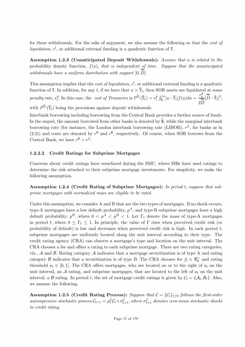
for these withdrawals. For the sake of argument, we also assume the following so that the cost of

liquidation, cl, or additional external funding is a quadratic function of T.

Assumption 1.2.3 (Unanticipated Deposit Withdrawals): Assume that u is related to the

probability density function, f(u), that is independent of time. Suppose that the unanticipated

withdrawals have a uniform distribution with support [0, D].

This assumption implies that the cost of liquidation, cl, or additional external funding is a quadratic

function of T. In addition, for any t, if we have that u > Tt, then SOR assets are liquidated at some

penalty rate, rpt . In this case, the cost of Treasuries is P Tt(Tt) = rpt∫∞

Tt[u−Tt]f(u)du =

rpt

2D[D−Tt]

2,

with P Tt(Tt) being the provisions against deposit withdrawals.

Interbank borrowing including borrowing from the Central Bank provides a further source of funds.

In the sequel, the amount borrowed from other banks is denoted by B, while the marginal interbank

borrowing rate (for instance, the London interbank borrowing rate (LIBOR), rL, for banks as in

(2.2)) and costs are denoted by rB and cB, respectively. Of course, when SOR borrows from the

Central Bank, we have rB = rL.

1.2.2.2 Credit Ratings for Subprime Mortgages

Concerns about credit ratings have resurfaced during the SMC, where SIBs have used ratings to

determine the risk attached to their subprime mortgage investments. For simplicity, we make the

following assumption.

Assumption 1.2.4 (Credit Rating of Subprime Mortgages): In period t, suppose that sub-

prime mortgages with normalized mass are eligible to be rated.

Under this assumption, we consider A and B that are the two types of mortgages. If no shock occurs,

type-A mortgages have a low default probability, pA, and type-B subprime mortgages have a high

default probability, pB, where 0 < pA < pB < 1. Let Γt denote the mass of type-A mortgages

in period t, where 0 ≤ Γt ≤ 1. In principle, the value of Γ rises when perceived credit risk (or

probability of default) is low and decreases when perceived credit risk is high. In each period t,

subprime mortgages are uniformly located along the unit interval according to their type. The

credit rating agency (CRA) can observe a mortgage’s type and location on the unit interval. The

CRA chooses a fee and offers a rating to each subprime mortgage. There are two rating categories,

viz., A and B. Rating category A indicates that a mortgage securitization is of type A and rating

category B indicates that a securitization is of type B. The CRA chooses fee ft ∈ ℜ+0 and rating

threshold at ∈ [0, 1]. The CRA offers mortgages, who are located on or to the right of at on the

unit interval, an A rating, and subprime mortgages, that are located to the left of at on the unit

interval, a B rating. In period t, the set of mortgage credit ratings is given by Ct = {At,Bt}. Also,we assume the following.

Assumption 1.2.5 (Credit Rating Process): Suppose that C = {Ct}t≥0 follows the first-order

autoregressive stochastic process Ct+1 = µCt Ct+σC

t+1, where σCt+1 denotes zero-mean stochastic shocks

to credit rating.

Page 17 of 179

The uncertainty in credit ratings before and after the SMC is encapsulated in this assumption.

1.2.2.3 Bank Regulatory Capital

For the purposes of our study, regulatory capital, K, is the value of SOR capital defined as the

difference between the accounting value of the assets and liabilities. More specifically, Tier 1

capital is represented by period t − 1’s market value of the SOR equity, ntEt−1, where nt is the

number of RMBS and Et is the period t market price of the SOR’s common equity. In our

contribution, period t, Tier 2 capital and Tier 3 capital are constituted by subordinate debt, Ot.

To maintain the book value feature of regulatory capital, it is assumed that last period’s market

value of equity and subordinate debt determines the capital constraint for the present period. The

balance sheet reflects the fact that SORs are active in the primary market by raising deposits,

D, from and extending credit, Λ, to the public. This involves transactions with other commercial

banks (interbank lending), with the Central Bank (monetary loans or deposits with the Central

Bank) and Treasury (buying and selling Treasury securities) as well as in the financial markets

(buying and selling risky marketable securities). Also the bank holds capital, K, as required by the

regulator, which serves as a cushion against unexpected losses (primarily from its loan portfolio).

In order to describe the binding capital constraint, we consider risk-weighted assets (RWAs) that

are defined by placing each on- and off-balance sheet item into a risk category. The more risky

assets are assigned a larger weight. Table 1.1 below provides RWA notation, Bank assets and their

probable risk-weights.

RWA Notation Bank Assets Risk-Weight

ωT Treasuries 0 %

ωB Structured Mortgage Products 20 %

ωM Mortgages 50 %

Table 1.1: Bank Assets and Their Risk Weights

As a result, RWAs are a weighted sum of the various assets of the SORs. In particular, we can

identify a special risk-weight on SOR’s loans, ωΛ = ω(Ct), that is a decreasing function of current

credit rating so that

∂ω(Ct)∂Ct

< 0.

This is in line with the procyclical notion that before the SMC, when credit ratings were high, the

risk-weights were low. On the other hand, during the SMC, risk-weights increased because of an

elevated probability of default and/or loss given default on loans. From [48] (see, also, [28]), SOR’s

total capital constraint is given by

Kt = ntEt−1 + Ot ≥ ρ

[ω(Ct)Λt + ωBBt + 12.5(mV aR+ O)

], (1.3)

Page 18 of 179

where ρ is the regulatory ratio of regulatory capital to risk-weighted assets. The nett cash flow

generated by SOR is given by the identity

Nt = Πt −∆Ft = ntdt + (1 + rOt )Ot − Kt+1 + ntEt, (1.4)

where Π is SOR’s profit under market value, ∆F is depreciation, d is dividends paid by SOR and

rO is the interest rate on period t subordinate debt.

1.2.2.4 A Valuation Problem for Subprime Mortgages

In our case, SOR faces a Hicksian demand for subprime mortgages given by


t .

where rΛt is the loan rate, Ct is a variable representing the credit rating (as a proxy for the level

of macroeconomic activity via procyclicality) and σΛt represents a random exogenous shock to the

demand for loans, which is defined over the interval [Λ,Λ]. We consider the possibility that MRs can

default on their principal payment. Moreover, the proportion of defaulted debt is assumed to be

a negative function of current credit ratings (macroeconomic conditions), i.e., write-offs are higher

when credit ratings are low than when they are high. SOR loan defaults translate into an extra

cost term in SOR’s profit function. As will become clear, the marginal cost curve will now shift

downwards (upwards) as credit ratings increase (decrease). In other words, economic conditions

affect loan supply as well as demand.

Another assumption introduced is that the risk-weight assigned to mortgages in the capital ade-

quacy ratio (CAR) is not constant, but is a decreasing function of current credit ratings, as implied

by Basel II. For the function

Jt = Πt + lt

[Kt − ρ

(ω(Ct)Λt + ωBBt + 12.5(mV aR+ O)

)](1.5)

−cdwt

[Kt+1

]+Et

[δt,1V

(Kt+1, xt+1

)],

the optimal SOR valuation problem is to maximize the value of SOR by choosing rΛ, D, T, and K,

for

V (Kt, xt) = maxrΛt , Dt, Tt

Jt, (1.6)

subject to the loan demand, balance sheet, cash flow and financing constraints given by

Page 19 of 179


t , (1.7)

Tt = (1− γ)Dt + Bt + ntEt−1 + Ot − Bt − Λt, (1.8)

Πt =

(rΛt − cΛωt

)Λt + rTt Tt − P T(Tt) +

(rBt − cBt

)Bt −

(rDt + cDt

)Dt (1.9)

−(rBt + cBt

)Bt,

and

Kt+1 = nt(dt + Et) + (1 + rOt )Ot − Πt +∆Ft, (1.10)

respectively. In the value function, lt is the Lagrange multiplier for the capital constraint, cdwt is

the deadweight cost of capital and δt,1 is a stochastic discount factor. In the profit function, cΛω is

the constant marginal cost of loans (including the cost of monitoring and screening).

The interest rate on deposits rD is assumed to follow first-order autoregressive stochastic processes

rDt+1 = µrD

t rDt + σrD

t+1,

where σrD

t+1 is a zero-mean stochastic shock to deposit rate.

The main result from [48] is as follows. Suppose that J and V are given by (1.5) and (1.6),

respectively. When the capital constraint given by (1.3) holds (i.e., lt > 0), a solution to the

optimal bank valuation problem yields an optimal mortgage supply and mortgage rate of the form

Λ∗t =

Kt

ρω(Ct)− ωBBt + 12.5(mV aR+ O)

ω(Ct)(1.11)

and

rΛ∗t =1

λ1

(λ0 + λ2Ct + σΛ

t − Kt

ρω(Ct)+

ωBBt + 12.5(mV aR+ O)

ω(Ct)

), (1.12)

respectively. In this case, the corresponding optimal deposits, provisions for deposit withdrawals

and profits are given by

Page 20 of 179

D∗

t =1

(1− γ)

(D +

D

rpt

[rT

t + (rBt − cBt ) + (rBt + c

B

t)−1

1− γ(rDt + c

Dt )

]

+Kt

ρω(Ct)−

ωBBt + 12.5(mV aR + O)

ω(Ct)+ Bt − Kt − Bt

),

T∗t = D +D

rpt

[rTt + (rBt − cBt ) + (rBt + cBt )−

1

1− γ(rDt + cDt )

]

and

Π∗t =

(Kt

ρω(Ct)−

ωBBt + 12.5(mV aR + O)

ω(Ct)

)

{1

λ1

(λ0 −

Kt

ρω(Ct)+

ωBBt + 12.5(mV aR+ O)

ω(Ct)+ λ2Ct + σ

Λt

)

−

(cΛωt + (rDt + cDt ) 1

1−γ

)}−

((rDt + cDt ) 1

1−γ

)(Bt − Kt − Bt

)

+

(D + D

rpt

[rTt + (rBt − cBt ) + (rBt + cBt)−

11−γ

(rDt + cDt )

])(rTt − (rDt + cDt ) 1

1−γ

)

+

(rBt − cBt

)Bt −

(rBt + cBt

)Bt − P T(Tt),

respectively.

1.2.3 Preliminaries about Subprime Mortgage Securitization

We introduce a subprime mortgage model with default to explain the key aspects of mortgage

securitization.

Page 21 of 179

Originator Mortgage Insurer

Trustees

Underwriter

Credit Rating Agency

1.3c

Monoline Insurer

1.3d

Subprime Agents Subprime Banks Markets

Mortgagor

1.3E X

1.3F X

Servicer

1.3G

1.3H

Subprime

Originator

1.3K 1.3L

Subprime

Interbank

Lender

1.3I 1.3J

House

Appraiser

1.3A

1.3B

1.3a

Mortgage

Market

1.3O

1.3P

Mortgage

Broker 1.3b

1.3C

1.3D

Subprime

Dealer

Banks

& SPVs

1.3M 1.3N

1.3Q

1.3R

X X

SMP

Bond

Market

Subprime

Investing

Banks

1.3S

1.3T

1.3U

1.3V

Money/

Hedge Fund

Market

1.3W 1.3X

Figure 1.3: Diagrammatic Overview of a Subprime Mortgage Model With Default

Figure 1.3 presents a subprime mortgage model involving nine subprime agents, four subprime

Page 22 of 179

banks and three types of markets. As far as subprime agents are concerned, we note that circles

1.3a, 1.3b, 1.3c and 1.3d represent flawed independent assessments by house appraisers (HAs),

mortgage brokers (MBs), credit rating agencies (CRAs) rating SPVs and monline insurers (MLIs)

being rated by rating agencies, respectively. Regarding the former agent, the process of subprime

mortgage origination is flawed with house appraisers not performing their duties with integrity and

independence. According to [23] this type of fraud is the ”linchpin of the house buying transaction”

and is an example of operational risk. Also, the symbol X indicates that the cash flow stops as

a consequence of defaults. Before the SMC, HAs estimated house values based on data that

showed that the house market would continue to grow (compare with 1.3A and 1.3B). In steps

1.3C and 1.3D, independent MBs arrange mortgage deals and perform checks of their own while

SORs originate mortgages in 1.3E. Subprime MRs generally pay high mortgage interest rates to

compensate for their increased risk from poor credit histories (compare with 1.3F). Next, the

servicer (SR) collects monthly payments from MRs and remits payments to SDBs and SPVs. In

this regard, 1.3G is the mortgage interest rate paid by MRs to the SR of the reference mortgage

portfolios while the interest rate 1.3H (mortgage interest rate minus the servicing fee), is passed

by the SR to the SPV for the payout to SIBs. SOR mortgage insurers (SOMIs) compensate SORs

for losses due to mortgage defaults. Several subprime agents interact with the SPV. For instance,

the trustee holds or manages and invests in mortgages and SMPs for the benefit of another. Also,

the underwriter is a subprime agent who assists the SPV in underwriting new SMPs. Monoline

insurers (MLIs) guarantee SIBs’ timely repayment of bond principal and interest when an SPV

defaults. In essence, such insurers provide guarantees to SPVs, often in the form of credit wraps,

that enhance the credit rating of the SPV. They are so named because they provide services to only

one industry. These insurance companies first began providing wraps for municipal bond issues,

but now provide credit enhancement for other types of SMP bonds, such as RMBSs and CDOs. In

so doing, MLIs act as credit enhancement providers that reduce the risk of mortgage securitization.

SOR has access to subprime mortgage investments that may be financed by borrowing from the

subprime interbank lender (SIL), represented by 1.3I. The SIL, acting in the interest of risk-neutral

shareholders, either invests its deposits in Treasuries or in SOR’s subprime mortgage projects. In

return, SOR pays interest on these investments to SIL, represented by 1.3J. Next, the SOR deals

with the mortgage market represented by 1.3O and 1.3P, respectively. Also, the SOR pools its

mortgages and sells them to SDBs and/or SPVs (see 1.3K). The SDB or SPV pays the SOR an

amount which is slightly greater than the value of the reference mortgage portfolios as in 1.3L.

A SPV is an organization formed for a limited purpose that holds the legal rights over mortgages

transferred by SORs during securitization. In addition, the SPV divides this pool into sen, mezz

and jun tranches which are exposed to different levels of credit risk. Moreover, the SPV sells these

tranches as securities backed by subprime mortgages to SIBs (see 1.3N) that is paid out at an

interest rate determined by the mortgage default rate, prepayment and foreclosure (see 1.3M). Also,

SPVs deal with the SMP bond market for investment purposes (compare with 1.3Q and 1.3R).

Furthermore, SORs have securitized mortgages on their balance sheets, that have connections with

this bond market. SIBs invest in this bond market, represented by 1.3S and receive returns on

SMPs in 1.3T. The money market and hedge fund market are secondary markets where previously

issued marketable securities such as SMPs are bought and sold (compare with 1.3W and 1.3X).

SIBs invest in these short-term securities (see, 1.3U) to receive profit, represented by 1.3V. During

Page 23 of 179

the SMC, the model represented in Figure 1.3 was placed under major duress as house prices began

to plummet. As a consequence, there was a cessation in subprime agent activities and the cash flows

to the markets began to dry up. Thus, causing the whole subprime mortgage model to collapse.

We note that the traditional mortgage model is embedded in Figure 1.3 and consists of the agents,

MRs, SILs and SORs as well as the mortgage market. In this model, SIL lends funds to SOR

to fund mortgage originations (see, 1.3I and 1.3J). Home valuation as well as income and credit

checks were done by the SOR before issuing the mortgage. The SOR then extends mortgages and

receives repayments that are represented by 1.3E and 1.3F, respectively. The SOR also deals with

the mortgage market in 1.3O and 1.3P. When a MR defaults on repayments, the OR repossesses

the house.

1.2.3.1 Design of Subprime Mortgage Securitization

In this subsection, we discuss the main design features of subprime structured mortgage prod-

ucts such as RMBSs and RMBS CDOs. In particular, we provide a description of SPVs, cost of

mortgages, default, collateral, adverse selection and residual value (see Chapter 3 for more details).

In terms of the organization of the SPV, there are various states that can be associated with

corporate forms such as a trust (denoted by E1), a limited liability corporation (LLC; denoted by

E2), LLP (E3) or a C-corporation (E4). Our interest is mainly in E1 trusts and E2 LLCs that have

their own unique tax benefits and challenges as well as degree of mortgage protection and legal

limited liability. For our purposes, the optimal state during the lifetime of Ei, i ∈ {1, 2} is denoted

by E∗, such that the deviation from E∗ is given by

∣∣Eit − E∗∣∣ .

These deviations measure the loss and opportunity costs arising from the use of suboptimal corpo-

rate structures such as SPVs. Usually such loss is in the form of increased legal fees, losses due to

low limited liability and the value of additional time spent in dispute resolution. In this case, the

formula for E is given by

Et = max{∣∣Eit − E∗

∣∣ , 0}. (1.13)

SOR’s may monitor MR activities to see whether they are complying with the restrictive agreements

and enforce the agreements if they are not by making sure that MRs are not taking on risks at

their expense. Securitization dissociates the quality of SOR’s original mortgage portfolio from the

quality of the cash flows from SOR’s reference mortgage portfolio, fΣM, to SIBs, where fΣ is the

fraction of the face value of mortgages, M, that is securitized. Whether on-balance sheet or in

the market, the weighted average of the cost of mortgages summarizes the cost of various funding

solutions. It is the weighted average of cost of equity and debt on SOR’s balance sheet and the

weighted average of the costs of securitizing various mortgages. In both cases, we use the familiar

weighted average cost of capital. As a consequence, cost of funds via securitization, cMΣω (includes

Page 24 of 179

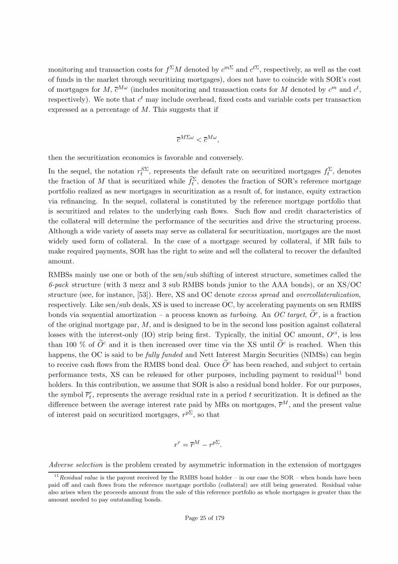
monitoring and transaction costs for fΣM denoted by cmΣ and ctΣ, respectively, as well as the cost

of funds in the market through securitizing mortgages), does not have to coincide with SOR’s cost

of mortgages for M, cMω (includes monitoring and transaction costs for M denoted by cm and ct,

respectively). We note that ct may include overhead, fixed costs and variable costs per transaction

expressed as a percentage of M. This suggests that if

cMΣω < cMω,

then the securitization economics is favorable and conversely.

In the sequel, the notation rSΣt , represents the default rate on securitized mortgages fΣt , denotes

the fraction of M that is securitized while fΣt , denotes the fraction of SOR’s reference mortgage

portfolio realized as new mortgages in securitization as a result of, for instance, equity extraction

via refinancing. In the sequel, collateral is constituted by the reference mortgage portfolio that

is securitized and relates to the underlying cash flows. Such flow and credit characteristics of

the collateral will determine the performance of the securities and drive the structuring process.

Although a wide variety of assets may serve as collateral for securitization, mortgages are the most

widely used form of collateral. In the case of a mortgage secured by collateral, if MR fails to

make required payments, SOR has the right to seize and sell the collateral to recover the defaulted

amount.

RMBSs mainly use one or both of the sen/sub shifting of interest structure, sometimes called the

6-pack structure (with 3 mezz and 3 sub RMBS bonds junior to the AAA bonds), or an XS/OC

structure (see, for instance, [53]). Here, XS and OC denote excess spread and overcollateralization,

respectively. Like sen/sub deals, XS is used to increase OC, by accelerating payments on sen RMBS

bonds via sequential amortization – a process known as turboing. An OC target, Oc, is a fraction

of the original mortgage par, M, and is designed to be in the second loss position against collateral

losses with the interest-only (IO) strip being first. Typically, the initial OC amount, Oci, is less

than 100 % of Oc and it is then increased over time via the XS until Oc is reached. When this

happens, the OC is said to be fully funded and Nett Interest Margin Securities (NIMSs) can begin

to receive cash flows from the RMBS bond deal. Once Oc has been reached, and subject to certain

performance tests, XS can be released for other purposes, including payment to residual11 bond

holders. In this contribution, we assume that SOR is also a residual bond holder. For our purposes,

the symbol rrt , represents the average residual rate in a period t securitization. It is defined as the

difference between the average interest rate paid by MRs on mortgages, rM , and the present value

of interest paid on securitized mortgages, rpΣ, so that

rr = rM − rpΣ.

Adverse selection is the problem created by asymmetric information in the extension of mortgages

11Residual value is the payout received by the RMBS bond holder – in our case the SOR – when bonds have beenpaid off and cash flows from the reference mortgage portfolio (collateral) are still being generated. Residual valuealso arises when the proceeds amount from the sale of this reference portfolio as whole mortgages is greater than theamount needed to pay outstanding bonds.

Page 25 of 179

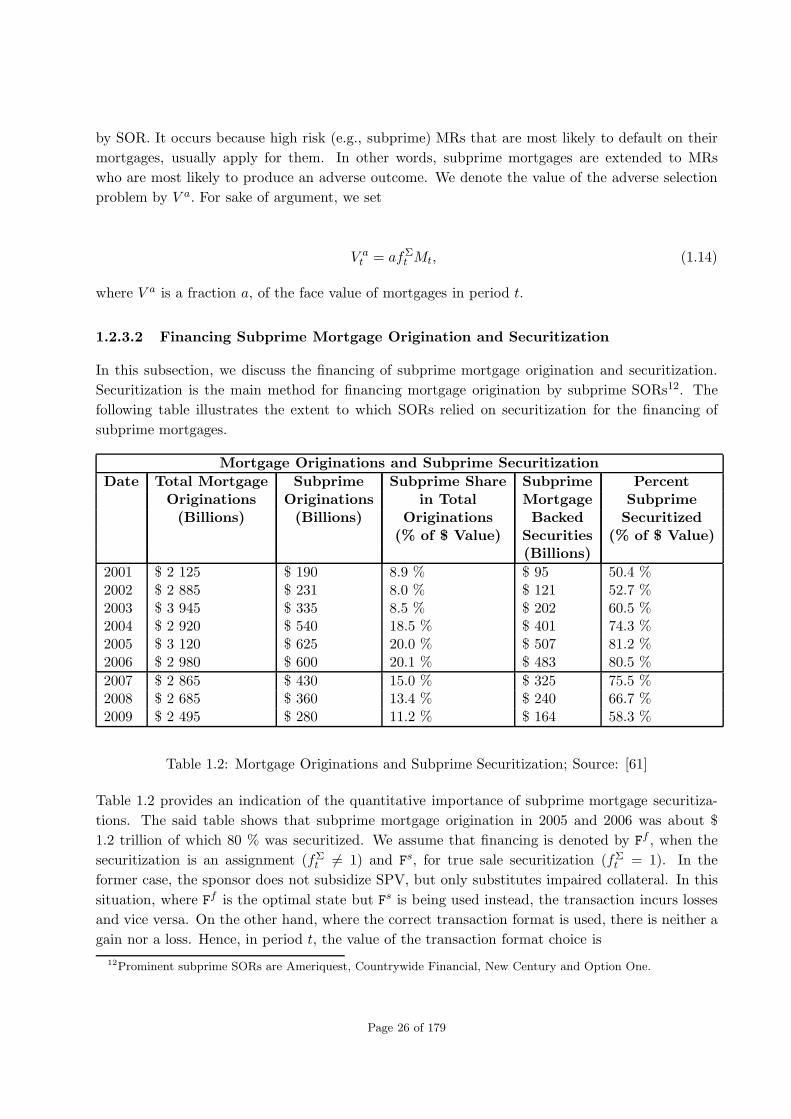
by SOR. It occurs because high risk (e.g., subprime) MRs that are most likely to default on their

mortgages, usually apply for them. In other words, subprime mortgages are extended to MRs

who are most likely to produce an adverse outcome. We denote the value of the adverse selection

problem by V a. For sake of argument, we set

V at = afΣ

t Mt, (1.14)

where V a is a fraction a, of the face value of mortgages in period t.

1.2.3.2 Financing Subprime Mortgage Origination and Securitization

In this subsection, we discuss the financing of subprime mortgage origination and securitization.

Securitization is the main method for financing mortgage origination by subprime SORs12. The

following table illustrates the extent to which SORs relied on securitization for the financing of

subprime mortgages.

Mortgage Originations and Subprime Securitization

Date Total Mortgage Subprime Subprime Share Subprime PercentOriginations Originations in Total Mortgage Subprime(Billions) (Billions) Originations Backed Securitized

(% of $ Value) Securities (% of $ Value)(Billions)

2001 $ 2 125 $ 190 8.9 % $ 95 50.4 %2002 $ 2 885 $ 231 8.0 % $ 121 52.7 %2003 $ 3 945 $ 335 8.5 % $ 202 60.5 %2004 $ 2 920 $ 540 18.5 % $ 401 74.3 %2005 $ 3 120 $ 625 20.0 % $ 507 81.2 %2006 $ 2 980 $ 600 20.1 % $ 483 80.5 %

2007 $ 2 865 $ 430 15.0 % $ 325 75.5 %2008 $ 2 685 $ 360 13.4 % $ 240 66.7 %2009 $ 2 495 $ 280 11.2 % $ 164 58.3 %

Table 1.2: Mortgage Originations and Subprime Securitization; Source: [61]

Table 1.2 provides an indication of the quantitative importance of subprime mortgage securitiza-

tions. The said table shows that subprime mortgage origination in 2005 and 2006 was about $

1.2 trillion of which 80 % was securitized. We assume that financing is denoted by Ff , when the

securitization is an assignment (fΣt 6= 1) and Fs, for true sale securitization (fΣ

t = 1). In the

former case, the sponsor does not subsidize SPV, but only substitutes impaired collateral. In this

situation, where Ff is the optimal state but Fs is being used instead, the transaction incurs losses

and vice versa. On the other hand, where the correct transaction format is used, there is neither a

gain nor a loss. Hence, in period t, the value of the transaction format choice is

12Prominent subprime SORs are Ameriquest, Countrywide Financial, New Century and Option One.

Page 26 of 179

Ft = max{∣∣∣Fft − Fst

∣∣∣ , 0}. (1.15)

1.2.4 Preliminaries About Subprime Risks

The main risks that arise when dealing with subprime residential mortgage products (RMPs) are

credit (including counterparty and default), market (including interest rate, price and liquidity),

operational (including house appraisal, valuation and compensation), tranching (including maturity

mismatch and synthetic) and systemic (including maturity transformation) risks. For sake of

argument, risks falling in the categories described above are cumulatively known as subprime risks.

In Figure 1.4 below, we provide a diagrammatic overview of the aforementioned subprime risks.

SubprimeRisks

Credit Risk

Market Risk

Operational Risk

Tranching Risk

Systemic Risk

Counterparty Risk

Default Risk

Interest Rate Risk

Price Risk

Liquidity Risk

House Appraisal Risk

Valuation Risk

Compensation Risk

Maturity Mismatch Risk

Synthetic Risk

Maturity Transformation Risk

Basis Risk

Prepayment Risk

Investment Risk

Re-investment Risk

Funding Risk

Credit Crunch Risk

Figure 1.4: Diagrammatic Overview of Subprime Risks

The most fundamental of the above risks is credit and market risk (refer to Subsections 3.6.1 and

3.6.2). The former involves SOR’s risk of loss from a MR who does not make scheduled payments

and its securitization equivalent. This risk category generally includes counterparty risk that, in

our case, is the risk that a banking agent does not pay out on a bond, credit derivative or credit

insurance contract (see, for instance, Subsection 3.6.1). It refers to the ability of banking agents –

such as SORs, MRs, servicers, SIBs, SPVs, trustees, underwriters and depositors – to fulfill their

obligations towards each other (see Section 3.6 for more details). During the SMC, even banking

agents who thought they had hedged their bets by buying insurance – via credit default swap (CDS)

Page 27 of 179

contracts or MLI insurance – still faced the risk that the insurer will be unable to pay.

In our case, market risk is the risk that the value of the mortgage portfolio will decrease mainly

due to changes in the value of securities prices and interest rates. Interest rate risk arises from

the possibility that subprime RMP interest rates will change. Subcategories of interest rate risk

are basis and prepayment risk. The former is the risk associated with yields on RMPs and costs

on deposits which are based on different bases with different rates and assumptions (discussed

in Subsection 3.6.2.2). Prepayment risk results from the ability of subprime MRs to voluntarily

(refinancing) and involuntarily (default) prepay their mortgages under a given interest rate regime.

Liquidity risk arises from situations in which a banking agent interested in selling (buying) RMPs

cannot do it because nobody in the market wants to buy (sell) those RMPs (see, for instance,

Subsections 3.6.1.2, 3.6.1.3 and 3.6.2.2). Such risk includes funding and credit crunch risk. Funding

risk refers to the lack of funds or deposits to finance mortgages and credit crunch risk refers to

the risk of tightened mortgage supply and increased credit standards. We consider price risk to be

the risk that RMPs will depreciate in value, resulting in financial losses, markdowns and possibly

margin calls that is discussed in Subsections 3.6.1.3 and 3.6.2.3. Subcategories of price risk are

valuation risk (resulting from the valuation of long-term RMP investments) and re-investment risk

(resulting from the valuation of short-term RMP investments). Valuation issues are a key concern

that must be dealt with if the capital markets are to be kept stable and they involve a great deal

of operational risk.

Operational risk is the risk of incurring losses resulting from insufficient or inadequate procedures,

processes, systems or improper actions taken (see, also, Subsection 3.6.1). As we have commented

before, for subprime mortgage origination, operational risk involves documentation, background

checks and progress integrity. Also, mortgage securitization embeds operational risk via mis-selling,

valuation and SIB issues. Operational risk related to mortgage origination and securitization results

directly from the design and intricacy of mortgages and related structured products. Moreover,

SIBs carry operational risk associated with mark-to-market issues, the worth of securitized mort-

gages when sold in volatile markets and uncertainty involved in investment payoffs. Also, market

reactions include increased volatility leading to behavior that can increase operational risk such as

unauthorized trades, dodgy valuations and processing issues. Often additional operational risk is-

sues such as model validation, data accuracy and stress testing lie beneath large market risk events

(see, for instance, [23]).

Tranching risk is the risk that arises from the intricacy associated with the slicing of securitized

mortgages into tranches in securitization deals (refer to Subsections 3.6.1.2 and 3.6.1.3). Pre-

payment, interest rate, price and tranching risk are also discussed in Subsection 3.6.4 where the

intricacy of subprime RMPs is considered. Another tranching risk that is of issue for RMPs is

maturity mismatch risk that results from the discrepancy between the economic lifetimes of RMPs

and the investment horizons of SIBs. Synthetic risk can be traded via credit derivatives – like CDSs

– referencing individual subprime RMBS bonds, synthetic CDOs or via an index linked to a basket

of such bonds. Synthetic risk is discussed in Subsection 3.6.2.2.

In banking, systemic risk is the risk that problems at one bank will endanger the rest of the

banking system (compare with Subsection 3.6.1). In other words, it refers to the risk imposed by

interlinkages and interdependencies in the system where the failure of a single entity or cluster

of entities can cause a cascading effect which could potentially bankrupt the banking system or

Page 28 of 179

market.

In Table 1.3 below, we identify the links in the chain of subprime risks with comments about the

information created and the agents involved.

Page 29 of 179

Chain of Subprime Risk and Securitization

Step in Chain Information Generated Agents Involved

Underwriting Standards;

Mortgage Mortgage Risk Characteristics;

Origination Credit Risk (Mortgage Quality); SORs & MBs

Operational Risk (Documentation,

Creditworthiness, Origination Process)

Reference RML Portfolio

Selected; RMBS Structured

Credit (Reference Portfolio) Risk; SDBs; SRs; CRAs;

Mortgage Securitization Market (Valuation, Liquidity) Risk; SIBs Buying Deal

Operational (Mis-selling, SIB Issues) Risk;

Tranching (Maturity Mismatch) Risk;

Systemic (Maturity Transformation) Risk;

ABS Portfolio Selected;

Manager Selected; CDO Structured

Securitization of ABSs, RMBSs, Credit (Reference Portfolio) Risk; SDBs; CDO Managers;

CMBSs into ABS CDOs; Market (Valuation, Liquidity) Risk; CRAs; SIBs Buying Deal

Operational (Mis-selling, SIB Issues) Risk;

Tranching (Maturity Mismatch) Risk;

Systemic (Maturity Transformation) Risk;

CDOs & Tranche Selected;

CDO Risk Transfer via Credit Risk in the form of SDBs; Banks with

CDSs in Negative Basis Trade Market (Basis) Risk Balance Sheets; CDOs

Credit (Counterparty) Risk

CDO Tranches Sale to CDOs & Tranche Selected SIV Manager; SIV Investors buy

SIVs & Other Vehicles; for SIV Portfolio SIV Liabilities

Market (Price and Interest Rate) Risk

Investment in SIV Liabilities Choice of SIV & Seniority Only Agents Directly

by Money Market Funds; Involved: Buyer & Seller

CDO Tranches Sale to Money CDOs & Tranche Selected Dealer Banks; Money Market

Market Funds via Liquidity Puts; Funds; Put Writers

Final Destination of Cash RMBS Only Agents Directly

Tranches, Cash CDO Tranches Location of Risk Involved: Buyer & Seller

& Synthetic Risk

Table 1.3: Chain of Subprime Risk and Securitization; Compare with [53]

Page30of179

Table 1.3 implies that IBs purchased tranches of structured products such as RMBSs, ABS CDOs,

SIV liabilities and money market funds without an intimate knowledge of the dynamics of the

products they were purchasing. These IBs likely relied on repeated relationships, bankers and on

credit ratings. Essentially, IBs do not have the resources to individually analyze such complicated

structures and, ultimately, rely to a lesser extent on the information about the structure and

the fundamentals and more on the relationship with the product seller. Agency relationships are

substituted for actual information. To emphasize this is not surprising, and it is not unique to

structured products such as RMBSs and ABS CDOs. However, in the SMC case, the length of the

chain of subprime risks is a huge problem.

1.2.5 Preliminaries about Subprime Data

In this subsection we discuss the different statistical techniques which are used for data analysis

such as time series analysis, linear regression, logit regression, hazard regression, t-statistic as well

as F-test. In this thesis, we consider data from LoanPerformance, ABSNET, Bloomberg, Lender

Processing Services (LPS), FHFA (Federal Housing Finance Agency) and the Federal Reserve

Bank of St Louis database as well as the Financial Service Research Program’s (FSRP) subprime

mortgage database for selected periods before and during the crisis. Additional parameter choices

are made by considering, for instance, [7], [34], [47], [53] and [105]. Some brief preliminaries about

time series analysis, linear and logit regression, the Cox-Proportional Hazard Model, t-statistic as

well as F -test are considered in the rest of this subsection.

1.2.5.1 Time Series Analysis

A Time series is a sequence of observations which are ordered in time (or space) and are best

displayed in a scatter plot. The series value X is plotted on the vertical axis and time t on the

horizontal axis. Time is the independent variable. There are two kinds of time series data:

(i) Continuous, where we have an observation at every instant of time. We denote this using

observation X at time t, X(t).

(ii) Discrete, where we have an observation at (usually regularly) spaced intervals. We denote this

as Xt.

Two main objectives of time series analysis are (i) identifying the nature of the phenomenon

represented by the sequence of observations, and (ii) predicting the future values of the time series

variable. Both of these objectives require that the pattern of observed time series data is identified

and more or less formally described.

Time series data have a natural temporal ordering, this makes time series analysis distinct from

other common data analysis problems. Time series trends in deal and mortgage characteristics for

subprime and Alt-A deals are given in Table 4.3 of Chapter 4.

1.2.5.2 Linear Regression

Linear regression is used to model the relationship between a scalar variable y and one or more

variables denoted X. Under this technique, if parameters of the models are unknown, they can be

Page 31 of 179

estimated from the data using linear models. Like all forms of regression analysis, linear regression

focuses on the conditional probability distribution of y given X, rather than on the joint probability

distribution of y and X, which is the domain of multivariate analysis.

Linear regression has many practical uses. Most applications of linear regression fall into one of

the following two broad categories:

1. If the goal is prediction, or forecasting, linear regression can be used to fit a predictive model

to an observed data set of y and X values. After developing such a model, if an additional value

of X is then given without its accompanying value of y, the fitted model can be used to make a

prediction of the value of y.

2. Given a variable y and a number of variables X1, . . . , Xp that may be related to y, then linear

regression analysis can be applied to quantify the strength of the relationship between y and the

Xj , to assess which Xj may have no relationship with y at all, and to identify which subsets of

the Xj contain redundant information about y, thus once one of them is known, the others are no

longer informative.

The most common method for fitting a regression line is the method of least-squares. This method

calculates the best-fitting line for the observed data by minimizing the sum of the squares of the

vertical deviations from each data point to the line (if a point lies on the fitted line exactly, then

its vertical deviation is 0). when the regression line is linear (y = ax+ b) the regression coefficient

is the constant a that represents the rate of change of one variable (y) as a function of changes in

the other (x); b is the slope of the regression line. Linear regression is used in Tables 4.6, 4.7, 4.8

and 4.9.

1.2.5.3 Logit Regression

Logit regression which can also be referred to as logistic or logit model is used to predict the proba-

bility of occurrence of an event by fitting data to a logit function (logistic curve). It is a generalized

linear model used for binomial regression. Like many forms of regression analysis, it makes use

of several predictor variables that may be either numerical or categorical. Logistic regression is a

technique for analyzing problems in which there are one or more independent variables that deter-

mine an outcome. Dependent variable is binary or dichotomous, i.e. it only contains data coded

as 1 (TRUE, success, etc.) or 0 (FALSE, failure, etc.).

The objective of logistic regression is to find the best fitting model to describe the relationship

between the dichotomous characteristic of interest (dependent variable = response or outcome

variable) and a set of independent (predictor or explanatory) variables. Logistic regression generates

the coefficients (and its standard errors and significance levels) of a formula to predict a logit

transformation of the probability of presence of the characteristic of interest:

logit(p) = b0 + b1X1 + b2X2 + b3X3 + ...+ bkXk

where p is the probability of presence of the characteristic of interest and b0, b1, b2, b3 ... bk are

the regression coefficients. The logit transformation is defined as the logged odds:

Page 32 of 179

odds =p

1− p=

probability of presence of characteristics

probability of absence of characteristics

and

logit(p) = ln

[p

1− p

]

Logit regression is used in Tables 4.4, 4.5, 4.12, 4.13 and 4.19.

1.2.5.4 Cox-Proportional Hazard Model

Proportional hazard models are a set of models that relate the time that passes before some event

occurs to one or more covariates that may be associated with the quantity. The models consist

of two parts, the underlying hazard function and the effect parameters. The underlying function

explains how the hazard (risk) changes over time at levels of covariates and the effect parameters

explains how the hazard varies in response to explanatory covariates.

Cox proportional-hazard regression allows analyzing the effect of several risk factors on survival.

The probability of the endpoint (death, or any other event of interest, e.g. recurrence of disease)

is called the hazard. The hazard is modeled as:

H(t) = H0(t)× exp(b1X1 + b2X2 + b3X3 + ...+ bkXk)

where X1, . . . , Xk are a collection of predictor variables and H0(t) is the baseline hazard at time

t, representing the hazard for a person with the value 0 for all the predictor variables.

ln

[H(t)

H0(t)

]= b1X1 + b2X2 + b3X3 + ...+ bkXk

where H(t)H0(t)

is the hazard ratio. The coefficients b1, b2, b3 ... bk are estimated by Cox regression,

and can be interpreted in a similar manner to that of multiple logistic regression. Hazard regression

is used in Tables 4.14, 4.15, 4.16 and 4.17.

1.2.5.5 t-Statistic

t-statistic is a parametric statistic whose sampling distribution is Student’s t-distribution. It is

defined by taking a statistic k, whose sampling distribution is a normal distribution, then subtract-

ing the expected value of the statistic (expected value is the sample mean µ), and dividing by an

estimate of its standard error (estimate of the error is the sample standard deviation s, divided by√n)

Page 33 of 179

t-statistic is given by,

t =k − µ(s/√n)

t-statistics are most frequently used in statistical hypothesis testing in Student’s t-tests and in the

computation of certain confidence intervals. The key property of the t-statistic is that it is a pivotal

quantity - while defined in terms of the sample mean, its sampling distribution does not depend

on the sample parameters, and thus it can be used regardless of what these parameters may be.

t-statistics is used in Tables 4.12, 4.13, 4.14, 4.15, 4.16, 4.17 and 4.19.

1.2.5.6 F -Test

F -test is a statistical test in which the test statistic has an F -distribution under the null hypothesis.

F -test is used when the sample size is small, i.e., n < 30. Exact F -tests mainly arise when the

models have been fit to the data using least squares. F -test is used to test the hypothesis that the

population variances are equal. It does this by comparing the ratio of two variances. So, if the

variances are equal, the ratio of the variances will be 1. The formula for F is simply

F =s21s22

The variance are arranged so that F > 1. That is; s21 > s22. F -test plays an important role in

the analysis of variance (ANOVA). The calculated value of the F -test with its associated p-value

is used to infer whether one has to accept or reject a null hypothesis. If the associated p-value

is small i.e. (< 0.05) we say that the test is significant at 5 % and we reject the null hypothesis

and accept the alternative one. On the other hand if associated p-value of the test is > 0.05, we

accept the null hypothesis and reject the alternative. Evidence against the null hypothesis will be

considered very strong if p-value is less than 0.01. In that case, we say that the test is significant

at 1%. F-test is used in Tables 4.5 and 4.9.

1.3 Main Problems, General Questions and Outline of the Thesis

In this section, we identify the main problems solved and give an outline of the thesis. Our general

objective is to investigate aspects of subprime mortgages and their securitization, Basel capital

regulation and their relationship with the SMC as well as subprime data.

1.3.1 Main Problems

The main problems that are solved in this thesis may be formulated as follows:

Problem 1.3.1 (Modeling of Subprime Mortgages): Can we model subprime mortgages that

are able to fully amortize, voluntarily prepay or involuntarily prepay (default) ? (see Subsection

2.2.2 of Section 2.2 in Chapter 2).

Page 34 of 179

Problem 1.3.2 (Traditional Mortgage Model with Subprime Elements for Capital, In-

formation, Risk, and Valuation): Can we construct a discrete-time traditional mortgage model

with subprime elements for capital, information, risk, and valuation incorporating costs of funds,

originator mortgage insurance and profits as well as mortgage defaults ? (see Subsection 2.3.1 of

Section 2.3 in Chapter 2).

Problem 1.3.3 (Optimal Valuation Problem Under Subprime Mortgages): In order to

obtain an optimal SOR valuation with subprime mortgages at face value which decisions regarding

mortgage rates, deposits and treasuries must be made ? (see Theorem 2.3.4 of Subsection 2.3.2 in

Chapter 2).

Problem 1.3.4 (Modeling of Capital, Information, Risk and Valuation Under Mort-

gage Securitization): Can we construct a discrete-time subprime mortgage model for capital,

information, risk and valuation that incorporates losses, monoline insurance, costs of funds and

profits under mortgage securitization ? (see Subsection 3.2.2 of Section 3.2 in Chapter 3).

Problem 1.3.5 (Optimal Valuation Problem Under Subprime Mortgage Securitiza-

tion): In order to obtain an optimal valuation under subprime mortgage securitization which de-

cisions regarding mortgage rates, deposits and treasuries must be made ? (see Theorems 3.2.4 and

3.3.3 of Subsections 3.2.4 and 3.3.3, respectively in Chapter 3).

Problem 1.3.6 (Mortgage Securitization Intricacy and Design Leading to Information

Problems, Valuation Opaqueness and Ineffective Risk Mitigation): Was the SMC partly

caused by the intricacy and design of subprime mortgage securitization that led to information (loss,

asymmetry and contagion) problems, valuation opaqueness and ineffective risk mitigation ? (see

Sections 3.2, 3.3, 3.4, 3.5 and 3.6 in Chapter 3).

Problem 1.3.7 (Mortgages and Capital Under Basel Regulation (Securitized Case)):

What is the effect of changes in credit ratings on SOR’s subprime mortgages and capital when the

mortgages are securitized ? (see Chapter 3).

Problem 1.3.8 (Basel Capital Regulation and the SMC): Did Basel capital regulation ex-

acerbate the SMC ? (see Chapter 3).

Problem 1.3.9 (Examples Involving Subprime Mortgage Securitization): Can we provide

appropriate examples to illustrate the main results about subprime mortgage securitization ? (see

Chapter 3).

Problem 1.3.10 (Examples Involving Subprime Data and the SMC): How does the data

about mortgages and structured mortgage products in the period before, during and after the SMC

illustrate the theory developed in Chapters 2, 3 ? (see Chapter 4).

Page 35 of 179

1.3.2 General Questions

This thesis specifically seeks to answer the questions posed in Problems 1.3.1 to 1.3.10 and a few

more general ones such as those listed below.

Question 1.3.11 (Risk Management Techniques): Why did contemporary risk management

techniques not contribute towards the mitigation of the SMC and its severity ?

Question 1.3.12 (Market Discipline and Regulation): Why didn’t market discipline and

regulation prevent the SMC ?

Question 1.3.13 (Causes and Consequences of the SMC): What were the root causes of the

SMC and what is its consequences for the real economy ?

Question 1.3.14 (Cures for the SMC): What short- and long-term policies will ultimately cure

the SMC ?

Question 1.3.15 (Prevention of Future Crises): What can prevent such a crisis from re-

occurring ?

1.3.3 Outline of the Thesis

The thesis is structured as follows. In Chapter 1, we present a brief literature review of SMC-related

banking issues such as subprime mortgages, liabilities, capital, profit and valuation. Furthermore,

we review relevant literature on the SMC and Basel capital regulation as well as the RMBS and

CDO processes. Here, for instance, we pay special attention to moral hazard and adverse selection

problems. Terse preliminaries about the main subprime mortgage-related issues mentioned above

are also provided. Chapter 1 includes the identification of specific problems to be solved in the

thesis. An outline of the chapters are given below.

1.3.3.1 Outline of Chapter 2: Subprime Mortgages

In Chapter 2, we start by looking at the background to subprime mortgage in Section 2.1 and

continue with subprime lending with our focus being on SOR’s interest rates, subprime mortgages

and LTVRs (see Section 2.2). Also, in Section 2.3, we investigate SOR’s capital, information, risk

and valuation under mortgage origination.

1.3.3.2 Outline of Chapter 3: Subprime Mortgage Securitization

Chapter 3 commences with a brief background to the securitization of subprime mortgages in

Section 3.1. In this regard, we consider a mechanism for subprime mortgage securitization, subprime

RMBS bonds as well as a motivating example for such securitization. This is followed by Section

3.2 that contains a discussion of an optimal profit problem under RMBSs. To make this possible,

capital, information, risk and valuation for a subprime mortgage model under RMBSs is analyzed.

An analogue of this under RMBS CDOs is achieved in Section 3.3. Furthermore, Section 3.5

Page 36 of 179

provides examples involving subprime mortgage securitization while Section 3.6 discusses some of

the key issues in this chapter. Finally, a 2007-2010 time-line and an appendix is provided in Sections

3.7 and 3.8, respectively.

Section 3.4 of Chapter 3 contains a discussion of the modeling issues related to the cyclicality of

bank credit and capital in a securitized context where risk-weights vary as in Basel regulation. Some

of the issues dealt with are the quantity and pricing of subprime RMBSs, RMBS CDOs as well

as bank capital under Basel regulation (see Subsection 3.4.1). Furthermore, Subsections 3.4.2 and

3.4.3 investigate subprime RMBSs and their rates in a securitized framework with slack and holding

constraints, respectively. We conclude Section 3.4 by examining the effect of a current credit rating

shock in future periods on subprime RMBSs, B, and RMBS payout rates, rB in Subsection 3.4.4.

1.3.3.3 Outline of Chapter 4: More Subprime Data

In Chapter 4, Section 4.1 we present the data from the papers [7] and [105]. The data presented

related to credit ratings of subprime and Alt-A mortgage backed security deals (see Subsection 4.1.1)

and foreclosure rates of portfolio and securitized mortgages (see Subsection 4.1.2). Furthermore

we analyze the data on each subsection presented in Section 4.1. The analysis can be found in

Subsections 4.2.1 and 4.2.2 of Section 4.2. We then conclude by investigating the connection the

presented data has with our models (see Sections 4.3).

1.3.3.4 Outline of Chapter 5: Conclusions and Future Directions

Chapter 5 presents a few concluding remarks and highlights some possible topics for future research.

1.3.3.5 Outline of Chapter 6: Bibliography

In Chapter 6, we list the articles, books and other sources that is cited in the thesis.

1.4 Format of the Thesis

In this section, we establish the format of the thesis. Chapters 2 to 4 each consist of background,

main sections, examples, discussions, a 2007-2010 timeline of SMC-related events as well as an

appendix.

1.4.1 Background

In each chapter, this subsection contains a background to the subject matter discussed in the

chapter. In particular, we consider the main features of the subprime activity to be studied as well

as a 2007-2010 timeline of events.

1.4.2 Main Sections

In each chapter, these sections contain the main results.

Page 37 of 179

1.4.3 Examples

In each chapter, this section contains numerical and illustrative examples of some of the main

results.

1.4.4 Discussions

This section is constituted by discussions of the main results and examples.

1.4.5 Timeline of SMC-Related Events

In each chapter, this section contains a timeline of SMC-related events involving the issues discussed

in the main results.

1.4.6 Appendix

This section contains additional information and proofs of the main results in each chapter.

Page 38 of 179

Chapter 2

Subprime Mortgages

”It’s now conventional wisdom that a housing bubble has burst. In fact, there were

two bubbles, a housing bubble and a financing bubble. Each fueled the other, but they

didn’t follow the same course.”

– Wall Street Journal, 2007.

”Certainly the underwriting standards for a large proportion of the U.S. home mortgages

originated in 2005 and 2006 would give most people a pause. The no-down payment,

no-documents and no-stated income-or-assets loans were unprecedented in the history

of mortgage finance and clearly ripe for abuse.”

– Prof. Linus Wilson (Louisiana at Lafayette), 2008.

”If a guy has a good investment opportunity and he can’t get funding, he won’t do it.

And that’s when the economy collapses.”

– Prof. Frederic Mishkin, 2008.

”Delinquency rates on commercial loans have doubled in the past year to 7 % as more

companies downsize and retailers close their doors, according to the Federal Reserve. In

some cases, originators are offering a temporary fix by granting mortgagors an extension

on loan maturities. On paper, that looks like a plus for the originator because the

mortgagor pays a fee or agrees to pay a higher interest rate, or both. This allows

originators to avoid having to foreclose or write down these loans as impaired assets.

They also can keep the loans on their books as nothing were amiss.”

– Rachel Beck reporting in the Washington Post on Saturday, 11 July 2009.

”For instance, on Friday, 14 September 2007, Northern Rock, the U.K.’s fifth-biggest

mortgage lender, started experiencing a bank run after it was revealed that the bank

was having trouble raising liquidity. Within one day, customers had withdrawn an

estimated £1 billion resulting in the first bank run in the U.K. since 1866. Earlier,

applying Basel II principles, Northern Rock announced it would boost its shareholder

dividend by 30 % - a step that depleted its capital even as regulators warned about the

39

lender’s condition. Adam Applegarth, Northern Rock’s CEO at the time of the crisis,

defended the lender’s dividend boosting before a parliamentary inquiry on the bank run.

He argued that because of the high credit quality of its RMLs in Basel II terms, the

lender could opt to hold less capital to cover potential losses. To finance its expansion,

Northern Rock began to borrow heavily in global financial markets, rather than relying

as much on traditional customer bank deposits. In fact, its deposits-to-total liabilities

and equity ratio had decreased from 63 % at the end of 1997 to 22 % at the end of 2006,

less than half the level of its fellow mortgage lenders. This meant that Northern Rock

had access to insufficient cash when its own liquidity dried up after investors decided to

stop financing its growth. Eventually, Northern Rock was nationalized by the British

government.”

– Adam Applegarth, Northern Rock, 2008.

KEYWORDS: House Prices; Loan-to-Value Ratio (LTVR); Subprime Originators (SORs); Mort-

gagors (MRs); Subprime Residential Mortgage Loans (RMLs); Mortgage Interest Rates; Credit

Risk; Credit Ratings Agency (CRA); Subprime Originator Mortgage Insurance (OMI); Subprime

Mortgage Crisis (SMC).

As was mentioned in Chapter 1, subprime residential mortgage lending involves mortgage origina-

tion to MRs who do not qualify for market interest rates because of income level, down payment size,

credit history and employment status. One of the most important aspects of subprime mortgages

is the impact of payment reset on the ability of MRs to make monthly repayments on schedule.

MRs may find that subprime mortgages are more demanding since subprime originators (SORs)

may charge higher interest rates, fees or penalties for late payments or prepayments. A subprime

mortgage is worse from SOR’s perspective because it is considered riskier than a prime mortgage

– with a higher probability of default - so SORs require those higher rates and fees to compensate

for additional risk. These mortgages can also be worse for all role players in the economy if this

risk does materialize. Such mortgages are designed in a way that enables MRs to repay mortgages

based on the appreciation of house prices. In reality, few other consumer mortgage designs have the

characteristic that the appreciation of an underlying asset (in our case, house prices) is so closely

associated with repayment capacity. Profit is a major indicator of financial crises for households,

companies and financial institutions. An example of this from the SMC, is that both the failure of

Lehman Brothers and the September 2008 acquisition of Merrill Lynch and Bear Stearns by Bank

of America and JPMorgan Chase, respectively, were preceded by a decrease in profitability and

an increase in the price of mortgages and their losses. We use the basic fact that profits can be

characterized as the difference between income and expenses that are reported in SOR’s income

statement. In our subsequent analysis, profit – along with regulatory capital – forms an important

component of valuation. The current chapter has strong connections with accomplished research

in [53], [84], [85] and [86].

Page 40 of 179

2.1 Background to Subprime Mortgages

In this section, we provide a background to subprime originators mortgage insurance (OMI) and

subprime mortgage agents for Chapter 2.

2.1.1 Subprime Originator Mortgage Insurance

SOR mortgage insurance (OMI) contracts involve one of the simplest insurances that can be used

to hedge against credit risk. An overview is provided in Figure 2.1 below.

Insurer

2.1A

OMI

Contract

2.1B

SOR

2.1C

XMortgagors

(MRs)

Figure 2.1: Overview of Originator Mortgage Insurance for Subprime Mortgages

In Figure 2.1, 2.1B is the OMI premium paid by SOR to the insurer. Moreover, 2.1A represents a

settlement by the insurer in the case of a credit event (fails to pay premium 2.1C or a credit-rating

downgrade occurs). In this case, the insurer covers SOR’s mortgage losses via 2.1A.

In this case, we make the following assumption.

Assumption 2.1.1 (Subprime Originator Mortgage Insurance Premium Rate): Assume

that the OMI premium rate is of the form

pit(C) = h(Γt(C),E[Ct(S)]), (2.1)

where Γt denote the mass of mortgages in period t, S is SOR’s mortgage losses and Ct is SOR’s

compensation for losses via the protection leg.

This assumption reflects the fact that credit ratings and expected mortgage losses have a role to play

in deciding the size of OMI premiums. In general, the OMI procedure follows the steps below. Step

1: SOR invests in mortgages which are risky. Step 2: SOR decides to hedge this risk by entering

into an OMI contract. Step 3: SOR makes periodic payments to the insurer. Step 4: If mortgages

default, the insurer will make a payment against losses faced by SOR. During the SMC some

financial institutions that sold OMIs failed to honor some of their obligations due to claim volume.

In particular, the insurance companies such as American International Group (AIG), Municipal

Bond Insurance Association (MBIA) and Ambac faced ratings downgrades because widespread

mortgage defaults increased their potential exposure to OMI losses (see, for instance [119]).

Page 41 of 179

2.1.2 The Economy, Economic Agents and Equilibrium

Throughout this chapter we consider an economy with periods, t − 1, t and t + 1, and two main

agents, viz., the subprime originator (SOR) and (subprime) mortgagor (MR). In the sequel, SOR

and MR are considered to be risk-neutral with stylized interactions. For setting the scene, we

assume the following.

Assumption 2.1.2 (Oligopolistic Market, Monopolistic Subprime Originator and Equi-

librium): SOR is assumed to operate in an oligopolistic market for subprime mortgages in which

there are several SORs that charge rM consistent with monopoly power. An individual SOR pre-

commits to a quantity of mortgages through its capital holding in period t and mortgage rate com-

petition follows in period t + 1. To characterize the equilibrium, we analyze the behavior of SOR

operating as a monopolist.

The assumption above implies that competition between monopolistic SORs are fixed in a oligopolis-

tic market. The pre-commitment assumption refers to the fact that the period t choice of capital

restricts mortgage in period t+ 1.

2.2 Subprime Mortgages Design

In the U.S., MR’s have the option to pay more than the required monthly payment (curtailment),

pay off the mortgage in its entirety (voluntary prepayment with the option of refinancing) or to

default (involuntary prepayment). The peculiar design features of subprime mortgages are discussed

below.

2.2.1 Mortgage Rates

SOR’s own mortgage rate, rMt , for profit maximizing SORs, may be determined as

rMt = rLt + t, (2.2)

where rLt is, for instance, the 6-month LIBOR rate and t is the risk premium.

Extending fully amortizing (two-period) mortgages to subprime MRs may be considered to be too

risky so that a mortgage design with special features are needed. In this regard, one of the most

important design features of subprime mortgages is payment reset and its impact on the ability

of MRs to repay their mortgages. This is understandable if one considers that more than 75 % of

the subprime mortgages extended in the period 2004–2006 were hybrid adjustable-rate mortgages

(ARMs)1. Here the payment reset effect is dependent on the severity of payment reset (depending

1Approximately 80 % of U.S. mortgages issued to subprime MRs in the five years up to 2008 were ARMs thatare complex financial instruments with payoff features similar to those of interest rate derivatives. By contrast to afixed-rate mortgage (FRM), MRs holding ARMs retain most of the interest rate risk, subject to a collar (floor andcap). Note that most MRs are not in a position to easily hedge away this interest rate risk. Mortgages are usuallyhybrid loans since they incorporate the features of both FRMs and ARMs. Another aspect is mortgage payment

Page 42 of 179

on rM and rL) as well as MR’s house equity at the time of reset (function of initial LTVR and

decreases in house prices, H) and market conditions. Before and during the SMC, for an initial

period t, low teaser rates, rε, were charged at the beginning of the mortgage term – that is typically

fixed for the first two (for 2/28 mortgages) or three (for 3/27 mortgages) years, and is lower than

what MRs would pay for a 30-year FRM. Subsequently, in period t+1, higher, market-based step-

up rates, rψ, were charged. As a consequence, for the adjustment periods t and t + 1 coinciding

with rε and a subsequent rψ, respectively, we have that

rM =

rǫt = rLt + ǫt, Period t;

rψt+1 = rLt+1 + ψt+1, Period t+ 1,

where ǫ and ψ are the risk premiums for rǫ and rψ, respectively.

2.2.2 Subprime Mortgages

We decompose the face value of subprime mortgages denoted by M into distinct components

that are fully amortizing, refinancing and defaulting. In this regard, in period t, we consider the

decomposition Mt = (1− rf − rS)Mt + rfMt + rSMt, where rf and rS are the fractions of M that

refinance and default, respectively. In period t, for nett subprime mortgage losses, S, we have that

St = (1− rRt )rSt Mt, where

Rt = min[aHt, rRt rSt Mt], a ∈ [0, 1], (2.3)

is the recovery amount. S increases when credit ratings, C, deteriorate according to∂St∂Ct

< 0. We

note that the above description of S is consistent with empirical evidence that suggests that losses

on subprime mortgage portfolios are correlated with credit ratings under any capital adequacy

regime (see, for instance, [48]).

From (1.2), we have that

Mt = m0 −m1rMt +m2Ct + σMt , (2.4)

where m0 = fMλ0, m1 = fMλ1 and m2 = fMλ2 with fM being the fraction of the face value of

SOR’s subprime mortgages to the mortgage demand of all SOR’s mortgages and λ0, λ1 and λ2

are as in (1.2) of Subsection 1.2.2.1. We note that M in (2.4) is an increasing function of C and a

decreasing function of rMt . Further, we make the next assumption.

reset that depends on a number of factors, including but not limited to: the amount of equity that these MRs havein their homes at the time of reset (which itself is a function of LTVR at origination and the severity of the declinein house prices), the severity of payment reset (which depends not only on the loan but also on the 6-month LIBORinterest rate), and of course conditions in the labor market.

Page 43 of 179

Assumption 2.2.1 (Random Shock to Mortgages): Assume that σMt is the random shock to

M with support [M,M ] that is independent of an exogenous stochastic variable, xt, to be charac-

terized below. Also, suppose that M follows the first-order autoregressive stochastic process

Mt+1 = µMt Mt + σMt+1, µMt = g(cMωt , pi(Ct)), (2.5)

where cMωt and pi(Ct) are the average weighted cost of mortgages and OMI premium rate, respec-

tively. Furthermore, σMt+1 denotes zero-mean stochastic shocks to the mortgage process.

In Assumption 2.2.1, equation (2.5) embeds the fact that mortgage losses, S(Ct), and OMI premium

rates, pi(Ct) ∈ [0, 1], (see (2.1)) are correlated with credit rating. As a result, if C decreases then

pi increases according to 0 ≤ pi(Ct) ≤ 1,∂pi(Ct)∂Ct

< 0. Empirical data supports the claim that pi

is correlated with credit ratings (see, for instance, [22] and [71]).

2.2.3 Subprime Loan-to-Value Ratios

For the purpose of subsequent discussions, in period t, we define the LTVR, L, by the formula

Lt =Mt

Ht, (2.6)

where M and H are the mortgage and house values, respectively. From the above formulation it

is clear that high L results from declining house prices that ultimately curtail the refinancing of

mortgages. On the other hand, low ratios imply favorable house equity for subprime MRs.

2.3 SubprimeMortgage Origination and its Connections with Cap-

ital, Information, Risk and Valuation

In this section, we firstly discuss SOR’s profit with subprime mortgages at face values and then

consider its valuation. In this context, we discuss a traditional mortgage model with subprime

elements for SOR’s profit and valuation. From (1.1), we are able to obtain a corresponding balance

sheet involving the face value of SOR’s subprime mortgages as

Mt +Bt + Tt = (1− γ)Dt + Bt +Kt, (2.7)

where M = fMΛ, B = fMB, T = fM T, D = fMD, B = fM B and K = fMK, with fM as

before. The rest of SOR’s balance sheet items are analogously defined. As a consequence of these

relationships, analogues of results for Λ can easily be obtained when attention is restricted to M.

Page 44 of 179

2.3.1 Risk and Profit Under Subprime Mortgages

In this subsection, we discuss SOR’s retained earnings and a traditional mortgage model with

subprime elements for SOR’s profit.

2.3.1.1 Retained Earnings Under Subprime Mortgages

We suspect that SOR’s profit, Π, is an increasing function of credit ratings, C, so that∂Πt∂Ct

> 0.

This is connected with procyclicality where profitability increased in the boom prior to the SMC,

when credit ratings increased. By contrast, profitability decreased during the SMC because of,

among many other factors, an increase in provisioning for bad mortgages.

To establish the relationship between bank profitability and the Basel Accord, a model of bank

financing is introduced that is based on [4]. In period t, we know that bank profits, Πt, are used

to meet SOR’s obligations that include dividend payments on equity, ntdt, where nt and dt are

the number of SOR’s shares and their dividends as well as interest and principal payments on

subordinate debt, (1 + rOt )Ot, where Ot is subordinate debt in the case where M is at face value.

The retained earnings, Ert , subsequent to these payments may be computed by using

Πt = Ert + ntdt + (1 + rOt )Ot. (2.8)

In standard usage, retained earnings refer to earnings that are not paid out in dividends, interest

or taxes. They represent wealth accumulating in the bank and should be capitalized in the value

of the bank’s equity. Retained earnings also are defined to include bank charter value income.

Normally, charter value refers to the present value of anticipated profits from future lending.

In each period, banks invest in fixed assets (including buildings and equipment) which we denote

by Ft. For simplicity, we assume the following.

Assumption 2.3.1 (Depreciation of Fixed Assets): Assume that SOR maintains fixed assets,

Ft, throughout its existence so that it must only cover the costs related to the depreciation of fixed

assets, ∆Ft.

These activities are financed through retaining earnings and the eliciting of additional debt and

equity, Et, so that

∆Ft = Ert + (nt+1 − nt)Et +Ot+1. (2.9)

We can use (2.8) and (2.9) to obtain an expression for bank capital of the form

Kt+1 = nt(dt + Et) + (1 + rOt )Ot −Πt +∆Ft, (2.10)

where Kt is defined by Kt = fMKt with K being defined as in (1.1).

Page 45 of 179

2.3.1.2 A Traditional Mortgage Model With Subprime Elements for Profit Under

Subprime Mortgages

A traditional mortgage model with subprime elements for SOR’s profit at face value can be built

by considering the difference between cash inflow and outflow. For this profit, in period t, cash

inflow is constituted by returns on risky marketable securities, rBt Bt, mortgages, rMt Mt, Treasuries,

rTt Tt, recovery amount, Rt, OMI protection leg payments, C(S(Ct)), and Πpt is the present value of

future profits from additional mortgages based on current mortgages. Furthermore, we consider the

cost of funds for M, cMωMt, face value of mortgages in default, rSt Mt, recovery value of mortgages

in default, rRt Mt, OMI premium, pi(Ct)Mt, the all-in cost of holding risky marketable securities,

cBt Bt, interest paid to depositors, rDt Dt, cost of taking deposits, cDt Dt, interest paid to borrowers,

rBt Bt, the cost of borrowing, cBtBt, provisions against deposit withdrawals, P T(Tt), and the value of

mortgage losses S(Ct), as cash outflow. Here rD and cD are the deposit rate and marginal cost

of deposits, respectively, while rB and cB are the borrower rate and marginal cost of borrowing,

respectively. In this case, we have that a traditional mortgage model with subprime elements for

SOR’s profit with all SOR’s mortgages at market value may be expressed as

Πt =

(rMt − cMω

t − pit + cpt rft − (1− rRt )r

St

)Mt + C(E[S(Ct)]) (2.11)

+

(rBt − cBt

)Bt + rTt Tt − P T(Tt)−

(rDt + cDt

)Dt −

(rBt + cBt

)Bt +Πpt .

Below we roughly attempt to associate different risk types to different cash inflow and outflow terms

in (2.11). We note that the cash inflow term rMt Mt embed credit and market risk (in particular,

interest rate risk) while cpt rftMt can be associated with market risk (in particular, prepayment risk).

Also, (rBt − cBt )Bt mainly embeds market risk. Furthermore, C(E[S(Ct)]) and Πpt involve at least

credit risk (particularly, counterparty risk) and market risk (more specifically, interest rate, basis,

prepayment, liquidity and price risk), respectively. In (2.11), the cash outflow terms cMωt Mt and

pi(Ct)Mt carry credit and operational risks. Also, (1 − rRt )rSt Mt carries credit and market risk

(including valuation risk). Deposit withdrawals, P T(Tt), carries systemic and market risk. Finally,

the term

(rBt + cBt

)Bt embeds market and credit risk. In reality, the risks that we associate with

each of the cash inflow and outflow terms in (2.11) are more complicated than presented above.

For instance, these risks are inter-related and may be strongly correlated with each other. All of

the above risk-carrying terms contribute to systemic risk that affects the entire banking system.

2.3.2 Valuation Under Subprime Mortgages

In this subsection, we discuss SOR’s nett cash flow and optimal valuation under subprime mort-

gages.

Page 46 of 179

2.3.2.1 Nett Cash Flow Under Subprime Mortgages

If the expression for retained earnings given by (2.8) is substituted into (2.9), SOR’s nett cash flow

generated is given by Nt = Πt −∆Ft = ntdt + (1 + rOt )Ot −Kt+1 + ntEt, where nt is the number

of shares in SOR’s equity. In addition, we have the relationship

Bank Value for a Shareholder = Nett Cash Flow + Ex-Dividend Bank Value

This translates to the expression Nt+Kt+1. Furthermore, the stock analyst evaluates the expected

future cash flows in j periods based on a stochastic discount factor, δt,j such that the value of the

bank is

Nt +Et

[ ∞∑

j=1

δt,jNt+j

]. (2.12)

2.3.2.2 Optimal Valuation Under Subprime Mortgages

In this subsection, we make use of the modeling of banking activities from previous discussions to

solve SOR’s optimal valuation problem. From [48], we have that SOR’s total capital constraint for

subprime mortgages at face value is given by

Kt = ntEt−1 +Ot ≥ ρ

[ω(Ct)Mt + ωBBt + 12.5fM (mV aR+ O)

], (2.13)

where ω(Ct) and ωB are the risk-weights related to SOR’s subprime mortgages at face value and

risky marketable securities, respectively, while ρ – Basel II pegs ρ at approximately 0.08 – is the

Basel capital regulation ratio of regulatory capital to risk-weighted assets. In order to state an

SOR’s optimal valuation problem, it is necessary to assume the following.

Assumption 2.3.2 (Subprime Originator’s Performance Criterion): Suppose that SOR’s

performance criterion, J, at t is given by

Jt = Πt + lt

[Kt − ρ

(ω(Ct)Mt + ωBBt + 12.5fM (mV aR+ O)

)](2.14)

−cdwt

[Kt+1

]+Et

[δt,1V

(Kt+1, xt+1

)],

where lt is the Lagrangian multiplier for the total capital constraint, Kt is defined by Kt = fMKt

with K being defined as in (1.1), Et[·] is the expectation conditional on the bank’s information

at time t and xt is the deposit withdrawals in period t with probability distribution f(xt). Also,

cdwt is the deadweight cost of total capital that consists of common and preferred equity as well as

subordinate debt, V is the value function with a discount factor denoted by δt,1.

Page 47 of 179

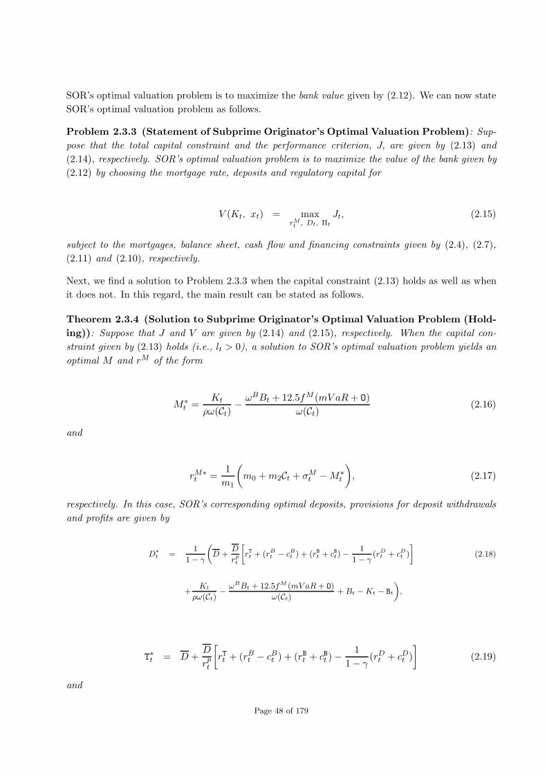
SOR’s optimal valuation problem is to maximize the bank value given by (2.12). We can now state

SOR’s optimal valuation problem as follows.

Problem 2.3.3 (Statement of Subprime Originator’s Optimal Valuation Problem): Sup-

pose that the total capital constraint and the performance criterion, J, are given by (2.13) and

(2.14), respectively. SOR’s optimal valuation problem is to maximize the value of the bank given by

(2.12) by choosing the mortgage rate, deposits and regulatory capital for

V (Kt, xt) = maxrMt , Dt, Πt

Jt, (2.15)

subject to the mortgages, balance sheet, cash flow and financing constraints given by (2.4), (2.7),

(2.11) and (2.10), respectively.

Next, we find a solution to Problem 2.3.3 when the capital constraint (2.13) holds as well as when

it does not. In this regard, the main result can be stated as follows.

Theorem 2.3.4 (Solution to Subprime Originator’s Optimal Valuation Problem (Hold-

ing)): Suppose that J and V are given by (2.14) and (2.15), respectively. When the capital con-

straint given by (2.13) holds (i.e., lt > 0), a solution to SOR’s optimal valuation problem yields an

optimal M and rM of the form

M∗t =

Kt

ρω(Ct)− ωBBt + 12.5fM (mV aR+ O)

ω(Ct)(2.16)

and

rM∗t =

1

m1

(m0 +m2Ct + σMt −M∗

t

), (2.17)

respectively. In this case, SOR’s corresponding optimal deposits, provisions for deposit withdrawals

and profits are given by

D∗

t =1

1− γ

(D +

D

rpt

[rT


B

t)−1

1− γ(rDt + c

Dt )

](2.18)

+Kt

ρω(Ct)−

ωBBt + 12.5fM (mV aR+ O)

ω(Ct)+Bt −Kt − Bt

),

T∗t = D +D

rpt


1

1− γ(rDt + cDt )

](2.19)

and

Page 48 of 179

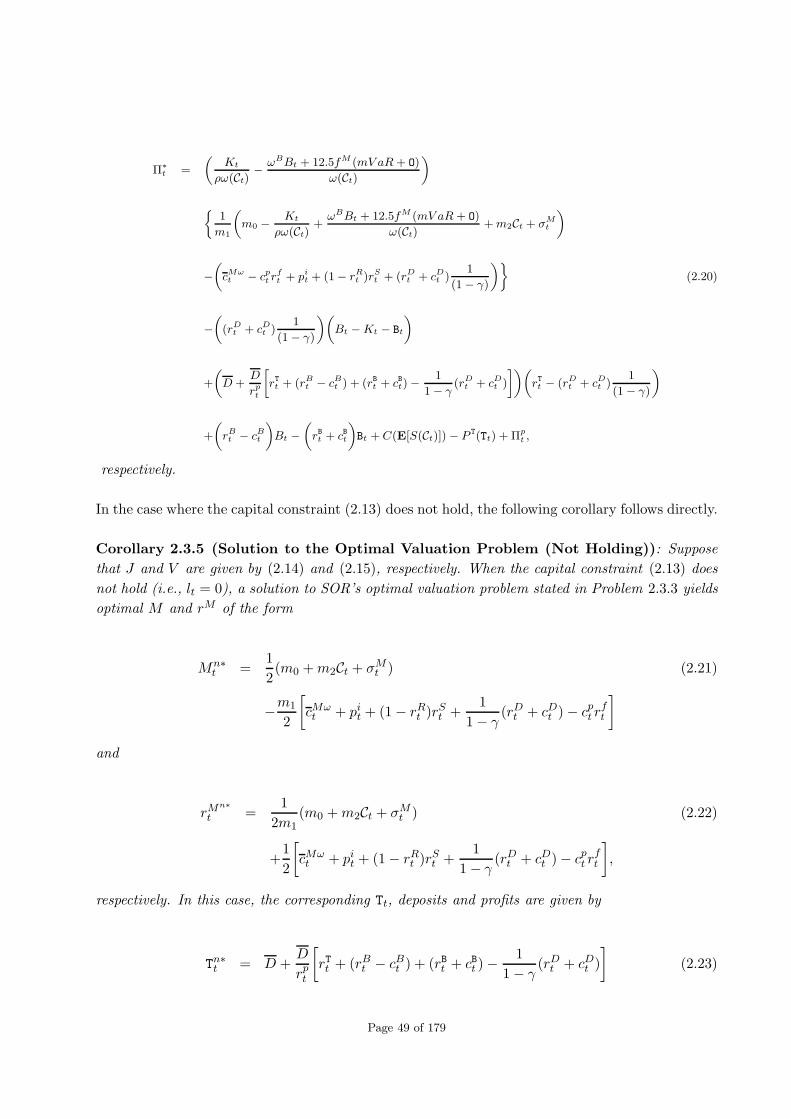
Π∗

t =

(Kt

ρω(Ct)−

ωBBt + 12.5fM (mV aR + O)

ω(Ct)

)

{1

m1

(m0 −

Kt

ρω(Ct)+

ωBBt + 12.5fM (mV aR + O)

ω(Ct)+m2Ct + σ

Mt

)

−

(cMωt − c

pt r

ft + p

it + (1− r

Rt )r

St + (rDt + c

Dt )

1

(1− γ)

)}(2.20)

−

((rDt + c

Dt )

1

(1− γ)

)(Bt −Kt − Bt

)

+

(D +

D

rpt

[rT


B

t)−1

1− γ(rDt + c

Dt )

])(rT

t − (rDt + cDt )

1

(1− γ)

)

+

(rBt − c

Bt

)Bt −

(rB

t + cB

t

)Bt +C(E[S(Ct)])− P

T(Tt) + Πpt ,

respectively.

In the case where the capital constraint (2.13) does not hold, the following corollary follows directly.

Corollary 2.3.5 (Solution to the Optimal Valuation Problem (Not Holding)): Suppose

that J and V are given by (2.14) and (2.15), respectively. When the capital constraint (2.13) does

not hold (i.e., lt = 0), a solution to SOR’s optimal valuation problem stated in Problem 2.3.3 yields

optimal M and rM of the form

Mn∗t =

1

2(m0 +m2Ct + σMt ) (2.21)

−m1

2

[cMωt + pit + (1− rRt )r

St +

1

1− γ(rDt + cDt )− cpt r

ft

]

and

rMn∗

t =1

2m1(m0 +m2Ct + σMt ) (2.22)

+1

2


St +

1


ft

],

respectively. In this case, the corresponding Tt, deposits and profits are given by

Tn∗t = D +D

rpt


1

1− γ(rDt + cDt )

](2.23)

Page 49 of 179

Dn∗t =

1

1− γ

(D +

D

rpt


1

1− γ(rDt + cDt )

](2.24)

+Mn∗t +Bt −Kt − Bt

).

and

Πn∗t =

(1

2(m0 +m2Ct + σMt )

−m1

2


St +

1


ft

])

{1

2m1(m0 +m2Ct + σMt )

−1

2


St +

1


ft

]}

−((rDt + cDt )

1

1− γ

)(Bt −Kt − Bt

)+

(D (2.25)

+D

rpt


1

1− γ(rDt + cDt )

])

(rTt − (rDt + cDt )

1

1− γ

)+

(rBt − cBt

)Bt −

(rBt + cBt

)Bt

+C(E[S(Ct)])− P T(Tt) + Πpt ,

respectively.

2.3.3 Optimal Valuation and Loan-to-Value Ratios

In this subsection, we connect the results from Subsection 2.3.2 with LTVRs, subprime mortgage

rates and prepayment costs. The following corollary about LTVRs follows immediately from The-

orem 2.3.4.

Corollary 2.3.6 (Loan-to-Value Ratios from Subprime Originator’s Optimal Valuation

Problem): Suppose that the hypothesis of Theorem 2.3.4 holds and that the LTVR is given by

(2.6). When lt > 0, then the LTVR corresponding to the optimal M from (2.16) is given by

L∗t =

Kt

ρω(Ct)Ht− ωBBt + 12.5fM (mV aR+ O)

ω(Ct)Ht. (2.26)

Page 50 of 179

On the other hand, when lt = 0, then the LTVR corresponding to an optimal M from (2.21) is

given by

Ln∗t =1

2Ht(m0 +m2Ct + σMt )− m1

2Ht(2.27)


St +

1


ft

].

Proof. The proof follows from the hypotheses of Theorem 2.3.4 and Corollary 2.3.5.

The paper [41] provides a relationship between SOR’s subprime mortgage rate, rM , the LTVR, L,

and a prepayment cost, cp, by means of the simultaneous equations model

rMt = α0Lt + α1cpt + α2Xt + α3ZrM

t + ut

Lt = β1rMt + β2Xt + β3ZLt + vt

cpt = γ1rMt + γ2Xt + γ3Zcp

t + wt.

(2.28)

MRs typically have a choice of rM and L, while the choice of cp triggers an adjustment to rM .

Thus, L and cp are endogenous variables in the rM -equation. There is no reason to believe that

L and cp are simultaneously determined. Therefore, cp does not appear in the L-equation and

L does not make an appearance in the cp-equation. From [41], matrix X comprises exogenous

explanatory variables such as mortgage characteristics (owner occupied, mortgage purpose, doc-

umentation requirements); MR characteristics (income and Fair Isaac Corporation (FICO) score)

and distribution channel (broker origination). The last term in each equation ZrM , ZL or Zcp

comprises the instruments excluded from either of the other equations. [41] points out that the

model is a simplification with other terms such as type of interest rate, the term to maturity and

distribution channel possibly also being endogenous. Nevertheless, by consideration of simultaneity

in the choice of rM and cp, it is possible to address the issue of possible bias in estimates of the

effect of cp on rM .

The next result follows from Theorem 2.3.4 and relates the subprime mortgage rate, rM , prepayment

cost, cp and LTVR, L.

Corollary 2.3.7 (Subprime Mortgage Rate, Prepayment Cost and Loan-to-Value Ra-

tio): Suppose that the hypothesis of Theorem 2.3.4 holds and that (2.6) and (2.28) hold. On the

other hand, when lt = 0, then the LTVR corresponding to an optimal M from (2.21) and the

optimal prepayment cost are given by

L∗t =

β1

2m1(m0 +m2Ct + σMt ) +

β1

2

[(1− rRt )r

St +

1

1− γ(rDt + cDt ) (2.29)

+(cMωt + pit − cpt r

ft )

]+ β2Xt + β3ZL

t + vt,

Page 51 of 179

and

cp∗t =γ1

2m1(m0 +m2Ct + σMt ) +

1

2

[(1− rRt )r

St +

1

1− γ(rDt + cDt ) (2.30)

+(cMωt + pit − cpt r

ft )

]+ γ2Xt + γ3Zcp

t + wt,

respectively.

Derived equations in this chapter are applied in Chapter 3.

Page 52 of 179

Chapter 3

Subprime Mortgage Securitization

”The current credit crisis will come to an end when the overhang of inventories of newly

built homes is largely liquidated, and home price deflation comes to an end. That will

stabilize the now-uncertain value of the home equity that acts as a buffer for all home

mortgages, but most importantly for those held as collateral for residential MBSs. Very

large losses will, no doubt, be taken as a consequence of the crisis. But after a period of

protracted adjustment, the U.S. economy, and the world economy more generally, will

be able to get back to business.”

– Alan Greenspan, 2007.

”Although there are only a few studies, the evidence to date is consistent with the

experience of a quarter century of securitization working very well. The assertions of

the originate-to-distribute view simply are not consistent with what we know. The idea

that there is a moral hazard due to the alleged ability of originators to sell loans without

fear of recourse, and with no residual risk, also assumes that the buyers of these loans

are irrational. That may be but the irrationality, it turns out, had to do with the belief

that house prices would not fall.”

– Prof. Gary Gorton, Yale University, 2008.

”I view the rating agencies as one of the key culprits. . . . They were the party that

performed the alchemy that converted the securities from F-rated to A-rated. The

banks could not have done what they did without the complicity of the rating agencies.”

– Prof. Joseph Stiglitz, Columbia University, 2009.

KEYWORDS: Subprime Originators (SORs); Mortgagors (MRs); Subprime Investing Banks

(SIB); Credit Ratings Agency (CRA); Servicers (SRs); Special Purpose Vehicles (SPVs); Special

Investment Vehicles (SIVs); Residential Mortgage Loans (RMLs); Residential Mortgage-Backed

Securities (RMBSs); Collateralized Debt Obligations (CDOs); Asset-Backed Commercial Paper

(ABCP); Subprime Mortgage Crisis (SMC); Basel Capital Regulation; Slack Constraints; Holding

Constraints; Mortgage Quantity and Pricing.

53

Under normal circumstance, the securitization of mortgages is an efficient, incentive compatible

response to bankruptcy costs and capital requirements. However, when these securitized mortgages

are subprime, several problems arise. In this chapter, we investigate the structural features of

subprime RMBSs, CDOs and other structured notes. Our deliberations separately focus on capital,

information, risk and valuation under RMBSs and RMBS CDOs. With regard to the latter, this

chapter discusses credit (including counterparty and default), market (including interest rate, price

and liquidity), operational (including house appraisal, valuation and compensation), tranching

(including maturity mismatch and synthetic) and systemic (including maturity transformation)

risks.

This chapter also addresses issues related to bank capital regulation and the SMC. Some of the

world’s top banking experts spent nearly a decade designing regulation in the form of the Basel

capital accords to ensure the health of the global banking industry.

What if some of their suppositions were inaccurate ?

The possibility that this is true was debated during the SMC that started unraveling from 2007

onwards. This crisis in world financial markets, initiated by mortgage losses in the U.S., brought into

question the effectiveness of global credit rating policy, financial stability and financial regulation

such as the new Basel II capital adequacy framework for banks (see, for instance, [11]).

Chapter 3 supports the IDIOM hypothesis that postulates that the SMC was mainly caused by

the intricacy and design of subprime mortgage origination, securitization and systemic agents that

led to information (loss, asymmetry and contagion) problems and valuation opaqueness. As a

consequence, subprime agents could not implement effective risk management policies. This claim

is illustrated via several examples. More specifically, information was lost due to intricacy resulting

from an inability to look through the chain of mortgages and structured products – reference

mortgage portfolios and RMBSs, ABS CDOs, structured investment vehicles (SIVs) etc. This

situation was exacerbated by a lack of understanding of how subprime securities and structures are

designed and intertwined. It is our opinion that the interlinked or nested unique security designs

that were necessary to make the subprime market function resulted in information loss among SIBs

as the chain of structured products stretched longer and longer. Also, asymmetric information arose

because SIBs could not penetrate the portfolio far enough to make a determination of the exposure

to the financial sector. An additional problem involved information contagion that played a crucial

role in shaping defensive retrenchment in interbank as well as mortgage markets during the SMC.

The valuation opaqueness problem related to structured products results from the dependence of

valuation on house prices and its independence from the performance of the reference mortgage

portfolios. Finally, we claim that SMC partly resulted from mortgage agents’ appetite for rapid

growth and search for high yields – both of which were very often pursued at the expense of risk

mitigation practices. The subprime structure described above is unique to the SMC and will be

elaborated upon in the sequel.

Page 54 of 179

3.1 Background to the Securitization of Subprime Mortgages

In this section, we discuss the basic securitization mechanism, background to subprime RMBS

bonds (sen/sub 6-pack and XS/OC structures, lock-out and step-down provisions, delinquency and

loss triggers as well as RMBS principal and interest waterfalls), background to collateralized debt

obligations (CDOs) and other structured notes (design of CDOs as well as structured investment

vehicles (SIVs) and asset-backed commercial paper (ABCP)) and a motivating example for the

securitization of subprime mortgages.

3.1.1 Mechanism for Subprime Mortgage Securitization

Figure 3.1 below provides a diagrammatic overview of the structure of a subprime mortgage secu-

ritization as it is discussed in this thesis.

OR’s Balance SheetAssets

Securitiesand

Treasuries

UnsecuritizedRMLs

SPV

Securitized RMLs

Liabilities

Deposits and

Regulatory Capital

Sen Tranche

Mezz Tranche

Jun Tranche

Agents

Arranger

Servicer

Credit RatingAgency (CRA)

Investors

Figure 3.1: Diagrammatic Overview of a Subprime Mortgage Securitization Structure

Figure 3.1 shows that securitized mortgages are sliced into 3 tranches, viz., senior (usually AAA

rated and abbreviated as sen), mezzanine (usually AA, A, BBB rated and abbreviated as mezz)

and junior (equity) tranches (usually BB, B rated and unrated and abbreviated as jun) in order

of contractually specified claim priority. CRAs provide a rating for each tranche and necessary

information to investors to make them tradeable. Tranches have different risk-return profiles and

Page 55 of 179

different maturities. The securitized mortgages owned by SPV generate cash flows that serve to

pay RMBS bond holders. The arranger structures the transaction while the servicer takes care

of day-to-day operations during the lifetime of the RMBS deal. The SPV isolates the reference

mortgage portfolio from SOR. A non-recourse mortgage sale implies that SOR is not responsible

for losses by bond holders. The structuring of the RMBS deal relies on covenants that rule the

governance of the SPV during its lifetime.

3.1.2 Background to Subprime RMBS Bonds

Subprime mortgage securitization reflects the design of the subprime mortgages. This meant that

credit risk was spread in a particular way and that additional complexity arose when assessing the

relative value of a particular subprime RMBS. Importantly, credit risk from RMBSs is inextricably

linked to the particular bond and transaction structure of which it is a part. In this subsection, we

discuss RMBS bond structure as it pertains to sen/sub 6-Pack and XS/OC structures, lock-out and

step-down provisions, delinquency and loss triggers as well as principal and interest rate waterfalls.

3.1.2.1 Sen/Sub 6-Pack and XS/OC Structures

As was mentioned before, RMBSs mainly use one or both of the sen/sub shifting interest structure

– known as the 6-pack structure (with 3 mezz and 3 sub RMBS bonds junior to the AAA bonds)

– or XS/OC (excess spread/over-collateralization) structure (see, for instance, [13]). Figure 3.2

below displays these two types of RMBS deal structures.

XS/OC deals are more complicated than straight sen/sub deals. For instance, additional complexity

arises from the available funds cap (AFC) risk. Generally, RMBS bonds in XS/OC deals pay a

floating coupon, rB, while subprime reference mortgage portfolios (collateral) typically pay a fixed

rate, rM , until the reset date on hybrid ARMs. In this case, the risk that interest paid into the

deal from the reference mortgage portfolio, rM , is not sufficient to make coupon payments, rB , to

RMBS bond holders may arise. To mitigate this situation, the deal may be subject to an AFC.

Here, SORs receive interest as the minimum of the sum of the index rate, rL, (i.e., 6-month LIBOR)

and margin, , or the weighted average AFC, raω. Symbolically, this means that

rB = min[rL + , raω]. (3.1)

3.1.2.2 Lock-Out and Step-Down Provisions

The lock-out and step-down provisions are common structural features of RMBS deals. Subsequent

to deal initiation, the lock-out provision locks out the mezz and sub bonds from receiving principal,

1fΣM, and prepayments, 2fpfΣM, where 1 and 2 are the fraction of the reference mortgage

portfolio, fΣM, that is paid as principal to the RMBS bond and the fraction of the prepaying

Page 56 of 179

Collateral

Deal Collateral

Face Value

Total Principal

Payments

InterestPayments

Deal with6-Pack

Structure

AAAs

S1

AA “M1”

A “M2”

BBB “M3”

BB “B1”

B “B2”

N.R. “B3”

IO

Interest on

the Bonds

Deal withXS/OC

AAAs

S2

AA “M1”

A “M2”

BBB “M3”

XS. OC

Residual

Interest on

the Bonds

S1 = Classic 6-Pack Credit Enhancement

S2 = Excess-Spread O/C-Based Credit Enhancement

Figure 3.2: Sen/Sub 6-Pack Structure vs. XS/OC Structure; Source: UBS

reference mortgage portfolio, fpfΣM, that is paid as prepayment to the RMBS bond, respectively.

This means that during the lock-out period, amortization is sequential1. The lock-out period, and

other details, differ depending on the characteristics of the reference mortgage portfolio (collateral).

During the deal, the XS/OC feature of RMBSs leads to an accumulation of credit enhancement

(CE) equity from the reference portfolio itself. Prior to the step-down date, sen tranches receive

100 % of 1fΣM. When the sen bonds are completely amortized away, prepayments, 2fpfΣM,

continue to sequentially amortize, with the next class being the outstanding mezz bonds. After the

lock-out period, deals are allowed to step-down, i.e., principal payments, 1fΣM, can be distributed

to the sub tranches provided that CE limits are twice the original levels and the deal passes other

performance criteria, measured by triggers. The step-down date in an XS/OC deal is the latter of

a specified month (e.g., 36 months) and the date at which the sen CE reaches a specified level (e.g.,

52 %).

3.1.2.3 Delinquency and Loss Triggers

The allocation of CE over time depends on triggers that reflect the credit quality of the subprime

reference mortgage portfolios. Under certain circumstances, triggers will cause a reallocation of

1fΣM to protect or increase subordination levels. Generally speaking, the two types of triggers

are delinquency and loss triggers. A trigger is said to pass if the collateral does not breach the

specified constraints, and to fail if those conditions are hit or breached. If a trigger fails, 1fΣM

to mezz and sub bonds are delayed or stopped, preventing a reduction of CE for the sen bonds.

1Sequential amortization means that there is a sequential elimination of RMBS bond liabilities in regular paymentsover a specified period of time.

Page 57 of 179

Loss triggers are target levels of cumulative losses as of specific dates after the RMBS deal was

initiated. XS builds up throughout the deal with a CE threshold (target) level eventually being

attained. Once this threshold is breached, XS can be paid to the residual holder, thus becoming

unavailable to cover reference mortgage portfolio losses. The aforementioned triggers have many

complicated features2 that are partially explained, for instance, in [81], [80] and [79]. Moreover,

cross-collateralization may occur where some deals contain multiple mortgage types. In this regard,

after interest payments are made on RMBS bonds of one type, funds that remain can be used to

pay interest to bonds in another.

3.1.2.4 RMBS Principal and Interest Waterfalls

As is shown in Figure 3.3 (see, also, Figures 3.4 and 3.5), invariably principal waterfalls are paid

sequentially for the first 36 months. This means that all scheduled principal, 1fΣM, and prepay-

ments, 2fpfΣM, are utilized to repay the sen bond holders first, until they are paid in full. Then,

these payments go to the next senior RMBS bond holder until they are fully paid. This process

repeats itself until eventually all bond holders are fully compensated.

Monthly Mortgage Payments

M1 M2 M3 M4 . . .M10M11 M12 M13 . . .M20M21 M22 M23 . . .M30M31 M32 M33 . . .M40M41 M42 M43 . . .M50... ... ... ...

M1991 M1992 . . .M2000

$

M1 M2 M3 M4 . . .M10M11 M12 M13 . . .M20M21 M22 M23 . . .M30... ... ... ...

M991 M992 . . .M1000

$

Servicer

$ I

$ P

Accounts

Interest

ScheduledPrincipal &Prepayments

InterestPayments

”AAA”

min[rL + , ra]

”AA”

min[rL + , ra]

”A”

min[rL + , ra]

”BBB”

min[rL + , ra]

”BBB-”

min[rL + , ra]

ResidualExcessInterest

PrincipalPayments


”AAA”

”AA”

”A”

”BBB”

”BBB-”

Residual

Figure 3.3: Sample Subprime RMBS Payments; Source: [67]

2For example, the loss trigger in months 1-36 might be 3.75 %, rise to 6.75 % in months 37-50, 6.85 % in months51-72, and stay flat at 7.25 % thereafter.

Page 58 of 179

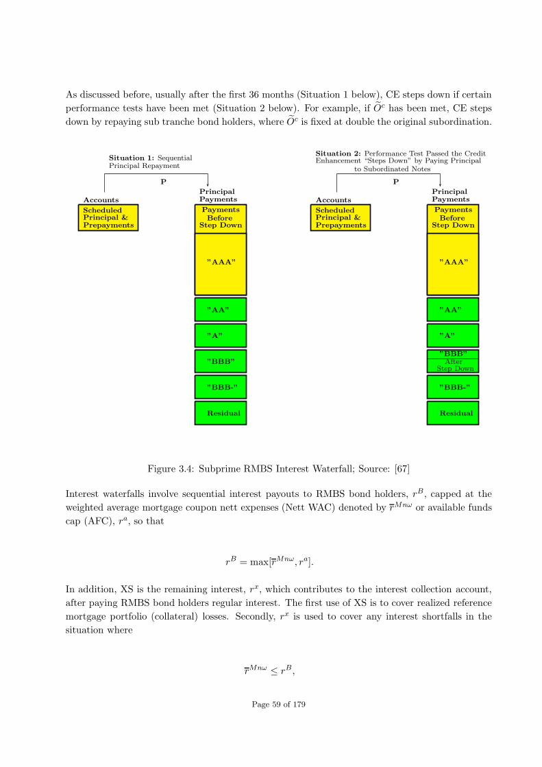
As discussed before, usually after the first 36 months (Situation 1 below), CE steps down if certain

performance tests have been met (Situation 2 below). For example, if Oc has been met, CE steps

down by repaying sub tranche bond holders, where Oc is fixed at double the original subordination.

Accounts


Situation 1: SequentialPrincipal Repayment

P

PrincipalPayments

PaymentsBefore

Step Down

”AAA”

”AA”

”A”

”BBB”

”BBB-”

Residual

Accounts


Situation 2: Performance Test Passed the CreditEnhancement “Steps Down” by Paying Principal

to Subordinated Notes

P

PrincipalPayments

PaymentsBefore

Step Down

”AAA”

”AA”

”A”

”BBB”After

Step Down

”BBB-”

Residual

Figure 3.4: Subprime RMBS Interest Waterfall; Source: [67]

Interest waterfalls involve sequential interest payouts to RMBS bond holders, rB , capped at the

weighted average mortgage coupon nett expenses (Nett WAC) denoted by rMnω or available funds

cap (AFC), ra, so that

rB = max[rMnω, ra].

In addition, XS is the remaining interest, rx, which contributes to the interest collection account,

after paying RMBS bond holders regular interest. The first use of XS is to cover realized reference

mortgage portfolio (collateral) losses. Secondly, rx is used to cover any interest shortfalls in the

situation where

rMnω ≤ rB ,

Page 59 of 179

with rMnω and rB as before. Lastly, the remaining XS accrues to the holder of the residual bond

which in our case is the subprime OR.

Accounts

Interest

$ I

Step 1-Interest PaidSequentially to Bonds,Capped at AFC

InterestPayments

”AAA”L+ % orNett WAC

”AA”L+ % orNett WAC

”A”L+ % orNett WAC

”BBB”L+ % orNett WAC

”BBB-”L+ % orNett WAC

ResidualExcessInterest

Step 2-ExcessInterest toCover CollateralLosses

PrincipalPayments


”AAA”

”AA”

”A”

”BBB”

”BBB-”

Residual

Losses

Step 3-RemainingExcess Interest toPay AFC Shortfalls

Interest

Shortfalls

L+ % -Nett WAC

L+ % -Nett WAC

Figure 3.5: Allocation of Interest; Source: [67]

3.1.3 Background to Collateralized Debt Obligations (CDOs)

RMBSs are usually bought by SIVs and ABCP conduits. In particular, SIVs issue short-term ABCP

and medium-term notes for purchase by money market funds and other risk-averse investors. The

returns from the sale of this paper and notes, in turn, fund the buying of collateral, including

structured notes. In essence, this means that long-term reference mortgage portfolios are converted

into supposedly less risky, shorter-term instruments. In addition, SIVs hold a large proportion of

CDOs that invest in asset-backed securities (ABSs) such as RMBSs (see, for instance, [67]).

3.1.3.1 ABS CDOs

As was the case for RMBSs in Subsection 3.1.2, ABS CDOs constitute a reference portfolio sliced

into tranches of differing risk-return profiles. SIVs assist hedge funds and banks to pool a number

of single RMBS tranches to create one CDO. As with RMBSs, risk associated with CDOs is shifted

from sen to sub tranches. The funds generated by the sale of CDOs enable CDO issuers to continue

Page 60 of 179

to underwrite the securitization of subprime mortgages or continue to purchase RMBSs. Major

depository banks around the world had also used financial innovations such as SIVs to circumvent

capital ratio regulations. This type of activity resulted in the failure of Northern Rock, which was

nationalized at an estimated cost of $ 150 billion.

We concentrate on ABS CDOs3 with underlying portfolios mainly constituted by RMBSs and

CMBSs. The chain formed by subprime mortgages, RMBSs and RMBS CDOs is portrayed in

Figure 3.6 below.

‘AAA’

‘AA’

‘A’

‘BBB’

‘BB.NR’

Risk Profile ofSubprime RMLs

BadGood

High

Low

Y

High GradeABS CDO

Senior ‘AAA’

Junior ‘AAA’

‘A’

‘BBB’

NR

‘AA’

Senior ‘AAA’

Junior ‘AAA’

‘A’

‘BBB’

NR

‘AA’

‘A’

‘BBB’

NR

‘AA’

SubprimeRMBsBonds

SubprimeRMLs

X

11 %

81 %

4 %

3 %

1 %, not all deals

14 %

62 %

8 %

6 %

6 %

4 %

27 %

60 %

4 %

3 %

3 %

2 %

Other Credit

Mezz ABS CDO (CDO)2

Enhancement:

Other Credit Enhancement:Excess Spread

Over-collateralization

X-axis = MR CreditY-axis = MR Down Payment

Excess Spread

Other CreditEnhancement:Excess Spread

5 %

88 %

3 %

2 %

1 %

1 %

Senior ‘AAA’

Junior ‘AAA’

Figure 3.6: Chain of Subprime Mortgages, RMBSs and RMBS CDOs; Source: UBS

As we proceed from left to right in Figure 3.6, subprime mortgages are securitized into RMBSs and

eventually RMBSs go into ABS CDOs. As far as the latter is concerned, it is clearly shown that

RMBS bonds rated AAA, AA, and A constitute the high grade CDO portfolio. On the other hand,

the BBB rated RMBS bonds are securitized into a mezz CDO, since its portfolio mainly consists of

BBB rated ABS and RMBS tranches. Moreover, if bonds issued by mezz CDOs are put into CDO

portfolios, then a type of CDO known as CDO squared or CDO2.

3By contrast, a cash CDO is a SIV that purchases fixed income asset portfolios that are financed via issuing sentranches (rated Aaa/AAA), mezz tranches (rated Aa/AA to Bb/BB) and jun tranches (unrated) – compare withRMBSs in Subsection 3.1.2. CDO portfolios usually included significant proportions of tranches of subprime andAlta-A deals.

Page 61 of 179

3.1.3.2 Features of ABS CDOs

There are some important features to ABS CDOs that make their design more complicated in the

subprime context. Most importantly, many cash ABS CDOs are managed, which means that there

is a manager that oversees the CDO portfolio. In particular, this manager is allowed to trade-buy

and sell-bonds, to a limited extent – say 10 % of the notional amount per year – over a limited

period of time – say the first 3 years of the transaction. The putative reason for this is that

structured products amortize, so to achieve a longer maturity for the CDO, managers need to be

allowed to reinvest. They can take cash that is paid to the CDO from amortization and reinvest

it, and with limitations, as mentioned, they can sell bonds in the portfolio and buy other bonds.

There are restrictions on portfolio that must be maintained, however. CDO managers typically

owned part or all of the CDO equity, so they would benefit from higher yielding assets for a given

liability structure. Essentially, think of a managed fund with term financing and some constraints

on the manager in terms of trading and portfolio composition. The restriction on the portfolio

composition would limit structured product asset categories to certain maximum amounts of the

portfolio. Other restrictions would include maximums and minimum by rating category, restrictions

on weighted average life (WAL), correlation factors, weighted average weighting factors (WARF),

numbers of obligors, etc.

3.1.3.3 Illustration of the Structure of ABS CDOs

Loss from any structured note depends on the aggregate level of losses in the reference mortgage

portfolio. Losses flow to structured notes according to their seniority. Another benefits from the

protection of all subordinate notes, whose total size determines the level of OC of the structured

note, characterizing its seniority. The total size of all sub notes under a specific note is a loss

franchise being the next senior tranche.

The loss allocation is very simple. A mortgage portfolio has a size 100. There are five types of

structured notes, each having an equal size of 20. A tranche becomes more senior as we move up

the structure. The lowest tranche is the jun tranche, sub 1 serving as equity for the other tranches

by being hit by any first loss of the reference mortgage portfolio. The most senior tranche is sen 3

(see Table 3.1 for more information).

Example of the Structuring of a CDO Note

Structured CDO Notes Value

sen 3 20sen 2 20sen 1 20mezz 1 20jun 1 20Total 100

Table 3.1: Example of the Structuring of a CDO Note

The exercise is to allocate loss. The reference mortgage portfolio loss can range from 0 up to 100

with a loss of 100 never happening. If the loss is lower than 20, it hits jun 1. If it is above the

Page 62 of 179

excess over 20 hits the next highest tranche, viz., mezz 1. Hence a 25 portfolio loss results in a

charge of 20 for jun 1 and 25 - 20 = 5 for mezz 1. Following the same rationale, the allocation of

a large portfolio loss of 45 would be 20 for jun 1, 20 for mezz 1, 5 for sen 1 and zero for both sen 2

and 3. Of course, the likelihood of these losses vary, with high losses exceptional and small losses

frequent.

3.1.4 Monoline Insurance for Subprime RMBSs and RMBS CDOs

In this subsection, a diagrammatic overview of SMPs being wrapped by an MLI is provided.

PROTECTION

SELLER

(i.e., MLI)

Monoline Insurer

3.7A

3.7B

3.7C

3.7D

3.7E

MLI Guarantee

MLI Premiums

Credit

Rating

Agency

PROTECTION BUYER

Subprime

Investing Bank

SUBPRIME

DEALER BANK

Special

Purpose Vehicle

SMP Bond

Purchase

SMP Bond

Principal & Interest

Figure 3.7: Structured Mortgage Products Wrapped by Monoline Insurance

The monoline insurance model in Figure 3.7 allows for (senior tranches of) SMPs to be wrapped

by MLIs. In this process, MLIs offer SIBs a guarantee on returns from SMP bonds (refer to 3.7A).

There are many reasons why such guarantees are viable in the real world. Differences in access to

information and in demand for credit risk are but two of them. To make this possible, the SPV –

the protection buyer – makes a regular stream of payments, to MLI in order to guarantee principal

and interest payments on the SMP bonds issued to SIB (see 3.7C). The effect of MLI insurance –

having the character of a guarantee - is that the risk premium on the bond shrinks thus reducing

the return SIBs receive (refer to 3.7D). However, the SPV has to pay a price for this as the MLI

premium must be paid. Before the SMC, given the low perceived risk of structured mortgage

products, MLIs generally have very high leverage, with outstanding guarantees often amounting to

150 times capital. In this type of insurance, default risk is transferred from the bondholders - in

Page 63 of 179

our case SIBs - to MLIs. SIBs are only left with the residual risk that the MLI will default. MLIs

carry enough capital to earn AAA ratings from CRAs and as a result often do not have to post

collateral (refer to 3.7E). As a consequence, MLIs make available SMP bonds easy to market, as

the credit risk is essentially that of the highly rated MLI simplifying analysis for most SIBs. In this

case, the analysis of the MLI is closely connected with the analysis of the default risk of all bonds

they insured.

3.1.5 Mortgage Securitization and Capital Regulation

Basel II aims to address weaknesses in the Basel I capital adequacy framework for banks by in-

corporating more detailed calibration of credit risk and by requiring the pricing of other forms of

risk such as operational risk. However, the 2007–2008 implementation of Basel II corresponded

to major losses suffered by some of the world’s major banks. Furthermore, the risk models that

underpin Basel II are similar to the ones many of those banks are currently using. Under the Basel

II framework, regulators allow large banks with sophisticated risk management systems to use risk

assessment based on their own models in determining the minimum amount of capital they are

required to hold by the regulators as a buffer against unexpected losses. Of concern is that by the

end of 2008, non risk-weighted capital adequacy ratios (CARs) were near historically low levels of

about 7.0 %. Naturally, these facts challenge the usefulness of important elements in the Basel II

accord.

At the beginning of 2008, it appeared that the SMC had caused a higher degree of problems for

non-U.S. financial institutions. The write-downs that British, European and Asian institutions had

to make on U.S. subprime mortgage debt was something that some analysts attributed to Basel

II that gave institutions some carte blanche when it came to raising capital for securities with top

credit ratings. Even in Switzerland, where Basel II was devised, regulators have questioned capital

regulation. For instance, UBS AG wrote down $ 18 billion in losses due to risk mismanagement and

exposure to subprime mortgages and other risky assets. In December 2007, UBS disclosed plans

to boost its capital with a $ 12.1 billion injection from the Government of Singapore Investment

Corp. and an unidentified Middle Eastern investor. In short, the Basel rules are being questioned

for containing inadequate prescriptions for monitoring a bank’s liquidity - in other words, its ability

to readily sell assets, or borrow affordably, to cover obligations. In principle, Basel II regulators

worldwide are required to track a bank’s risk-taking and to check how the bank monitors itself.

Traditionally, it is not their task to prescribe to banks about the size and type of risks they can take.

In the U.S., some regulators have recently shown a willingness to tighten Basel capital regulation.

They are motivated by the failure of more than 1 000 banks amid unforeseen risks related to interest

rates and real estate during the 1980’s S&L crisis. In addition, regulators both in the U.S. and

elsewhere are gearing themselves to amend Basel II. In all likelihood, this will involve enforcing a

higher level of capital against assets that may be construed to be risky in the wake of the SMC.

Undergirded by the analysis in [48], we extend aspects of the literature mentioned in Subsection

1.1 in several important directions. Firstly, in a Basel II framework, we investigate the dynamics

of bank capital and credit and their sensitivity to changes in the level of RMBS credit ratings.

Here mortgage risk-weights are kept constant and we consider credit and market risk as well as

operational risk. Next we include a discussion of subprime RMBSs and their reduced risk premiums.

Page 64 of 179

Finally, we consider the effect that Basel capital regulation has had on the SMC.

3.2 Risk, Profit and Valuation Under RMBSs

In this section, we provide more details about securitized mortgages and related issues such as risk,

profit and valuation. In the sequel, we assume that the notation Π, rM , M, cMω, pi, cp, rf , rR,

rS, S, C, C(E[S(C)]), rB, cB , B, rT, T, P T(T), rD, cD, D, rB, cB, B, Πp, K, n, E, O, ω(C), ωB, fM ,

mV aR and O corresponds to that of Subsection 2.3.1.2. Furthermore, the notation rSΣ, represents

the loss rate on securitized mortgages, fΣ, is the fraction of M that is securitized and fΣ denotes

the fraction of M, realized as new securitized mortgages, where fΣ ∈ fΣ. The following assumption

about the relationship between SIB’s and SOR’s profit is important for subsequent analysis.

Assumption 3.2.1 (Relationship between Subprime Originator and Subprime Invest-

ing Banks): We suppose that SIB and SOR share the same balance sheet given by (2.7). Further-

more, we assume that SIB is the only recipient of SORs securitized mortgages and that SIB’s profit

can be expressed as a function of the components of this securitization.

This assumption enables us to subsequently derive an expression for SIB’s profit under mortgage

securitization as in (3.2) from SOR’s profit formula given by (2.11).

3.2.1 Subprime RMBSs

The process of mortgage securitization into RMBSs takes a portfolio of illiquid mortgages – called

the reference mortgage portfolio – with high yields and places them into a SPV. To finance the

purchase of this portfolio, the SPV plans to issue highly rated bonds paying lower yields. The trust

issues bonds that are partitioned into tranches with covenants structured to generate a desired

credit rating in order to meet SIBs’ demand for highly rated assets. The usual trust structure

results in a majority of the bond tranches being rated investment grade. This is facilitated by

running the reference mortgage portfolio’s cash flows through a waterfall payment structure. The

cash flows are allocated to the bond tranches from the top down: the senior bonds get paid first,

and then the junior bonds, and then the equity. To insure a majority of the bonds get rated AAA,

the waterfall specifies that the senior bonds get accelerated payments (and the junior bonds get

none), if the reference mortgage portfolio appears to be under stress4. As was mentioned before,

this credit ratings can also be assured via the use of a MLI surety wrap. In addition, the super

senior tranches are often unfunded, making them more attractive to SIBs.

The costs related to mortgage securitization emanate from managerial time, legal fees and rating

agency fees. The RMBS equity holders would only perform securitization if the process generated

a positive nett present value. This could occur if the other tranches were mispriced. For example,

if AAA rated tranches added a new RMBS that attracted new sources of funds. However, asset

securitization started in the mid 1980s, so it is difficult to attribute the demand that we have

witnessed over the last few years for AAA rated tranches to new sources of funds. After this length

4Stress is usually measured by collateral/liability and cashflow/bond-payment ratios remaining above certaintrigger levels.

Page 65 of 179

of time, SIBs should have learnt to price tranches in a way that reflects the inherent risks. If

RMBS bond mispricing occurred, why ? The AAA rated liabilities could be over-priced due to

either mispricing liquidity or the rating of the SPV’s bonds were inaccurate.

3.2.2 Risk and Profit Under RMBSs

In this subsection, we discuss a subprime mortgage model for capital, information, risk and valua-

tion and its relation to retained earnings.

3.2.2.1 A Subprime Mortgage Model for Risk and Profit Under RMBSs

In this thesis, a subprime mortgage model for capital, information, risk and valuation under RMBSs

can be constructed by considering the difference between cash inflow and outflow. In period t, cash

inflow is constituted by returns on the residual from mortgage securitization, rrt fΣt f

Σt Mt, securi-

tized subprime mortgages, rMt (1− fΣt )f

Σt Mt, unsecuritized mortgages, rMt (1−fΣ

t )Mt, unsecuritized

mortgages that are prepaid, cpt rft (1 − fΣ

t )Mt, rT

t Tt, (rBt − cBt )Bt, as well as C(E[S(C)]) and the

present value of future gains from subsequent mortgage origination and securitizations, ΠΣpt . On

the other hand, in period t, we consider the average weighted cost of funds to securitize mortgages,

cMΣω fΣt f

Σt Mt, losses from securitized mortgages, rSΣt fΣ

t fΣt Mt, forfeit costs related to MLI insur-

ance wrapping RMBSs, ciΣt fΣt f

Σt Mt, transaction cost to extend mortgages, ctt(1 − fΣ

t )fΣt Mt, and

transaction costs from securitized mortgages ctΣt (1− fΣt )f

Σt Mt as part of cash outflow. Additional

components of outflow are weighted average cost of funds for extending mortgages, cMωt (1−fΣ

t )Mt,

MI premium for unsecuritized mortgages, pi(Ct)(1−fΣt )Mt, nett losses for unsecuritized mortgages,

(1− rRt )rSt (1− fΣ

t )Mt, decreasing value of adverse selection, afΣt Mt, losses from suboptimal SPVs,

Et and cost of funding SPVs, Ft. From the above and (2.11), we have that a subprime mortgage

model for profit under subprime RMBSs may have the form

ΠΣt =

(rrt − cMΣω

t − rSΣt − ciΣt

)fΣt f

Σt Mt +

(rMt − ctt − ctΣt

)(1− fΣ

t )fΣt Mt (3.2)

+

(rMt − cMω

t − pit(Ct) + cpt rft − (1− rRt )r

St

)(1− fΣ

t )Mt − afΣt Mt + rTt Tt

−(rBt + cBt

)Bt +

(rBt − cBt

)Bt −

(rDt + cDt

)Dt + C(E[S(Ct)])− P T(Tt)

+ΠΣpt − Et − Ft,

where ΠΣpt = Πpt + ΠΣ

t . Furthermore, by considering∂S(Ct)∂CBt

< 0 and (3.2), ΠΣ is an increasing

function of RMBS credit rating CB so that∂ΠΣ

t

∂CBt> 0. Furthermore, the MI forfeit cost term, ciΣ,

is a function of SPV’s MLI premium and payment terms.

Below we roughly attempt to associate different risk types to different cash inflow and outflow terms

in (3.2). We note that the cash inflow terms rrt fΣt f

Σt Mt and rMt (1− fΣ

t )fΣt Mt embed credit, market

Page 66 of 179

(in particular, interest rate), tranching and operational risks while rMt (1 − fΣt )Mt carries market

(specifically, interest rate) and credit risks. Also, cpt rft (1 − fΣ

t )Mt can be associated with market

(in particular, prepayment) risk while (rBt − cBt )Bt mainly embeds market risk. C(E[S(C)]) and

ΠΣpt involve at least credit (particularly, counterparty) and market (more specifically, interest rate,

basis, prepayment, liquidity and price), respectively. In (3.2), the cash outflow terms cMΣωfΣt f

Σt Mt,

ctt(1− fΣt )f

Σt Mt and ctΣt (1− fΣ

t )fΣt Mt involve credit, tranching and operational risks while cMω

t (1−fΣt )Mt and pi(Ct)(1− fΣ

t )Mt carry credit and operational risks. Also, rSΣt fΣt f

Σt Mt embeds credit,

market (including valuation), tranching and operational risks and ciΣt fΣt f

Σt Mt involves credit (in

particular, counterparty), tranching and operational risks. Furthermore, (1 − rRt )rSt (1 − fΣ

t )Mt

and afΣt Mt both carry credit and market (including valuation) risks. Finally, Et and Ft embed

credit (in particular, counterparty and valuation) and market and operational risks, respectively.

In reality, the risks that we associate with each of the cash inflow and outflow terms in (3.2) are

more complicated than presented above. For instance, these risks are inter-related and may be

strongly correlated with each other. All of the above risk-carrying terms contribute to systemic

risk that affects the entire banking system.

3.2.2.2 Profit Under RMBSs and Retained Earnings

As for SOR’s profit under mortgages, Π, we conclude that SIB’s profit under RMBSs, ΠΣ, are used

to meet its obligations, that include dividend payments on equity, ntdt. The retained earnings, Ert ,

subsequent to these payments may be computed by using

Πt = Ert + ntdt + (1 + rOt )Ot. (3.3)

After adding and subtracting

(rMt − cMω


St

)Mt from (3.2), we obtain

ΠΣt = Πt +

(rrt − cMΣω

t − rSΣt − ciΣt − rMt + ctt + ctΣt

)fΣt f

Σt Mt

+

(cMωt + pit + (1− rRt )r

St − ctt − ctΣt − cpt r

ft − a

)fΣt Mt − Et − Ft + ΠΣ

t .

If we replace Πt by using (3.3), ΠΣt is given by

ΠΣt = Er

t + ntdt + (1 + rOt )Ot +

(rrt − cMΣω


)fΣt f

Σt Mt (3.4)

+



ft − a


t .

From (2.10) and (3.4) we may derive an expression for SIB’s capital of the form

Page 67 of 179

KΣt+1 = nt(dt + Et)−ΠΣ

t +∆Ft + (1 + rOt )Ot +

(rrt − cMΣω

t − rSΣt − ciΣt − rMt (3.5)

+ctt + ctΣt

)fΣt f

Σt Mt +



ft − a

)fΣt Mt

−Et − Ft + ΠΣt .

where Kt is defined by (2.7).

3.2.3 Valuation Under RMBSs

If the expression for retained earnings given by (3.4) is substituted into (2.9), the nett cash flow

under RMBSs generated by SIB is given by

NΣt = ΠΣ

t −∆Ft

= nt(dt +Et)−KΣt+1 + (1 + rOt )Ot (3.6)

+

(rrt − cMΣω


)fΣt f

Σt Mt

+



ft − a


t .

We know that valuation is equal to SIB’s nett cash flow plus ex-dividend value. This translates to

the expression

V Σt = NΣ

t +KΣt+1, (3.7)

where Kt is defined by (2.7). Furthermore, the stock analyst evaluates the expected future cash

flows in j periods based on a stochastic discount factor, δt,j such that SIB’s value is

V Σt = NΣ

t +Et

[ ∞∑

j=1

δt,jNΣt+j

]. (3.8)

3.2.4 Optimal Valuation Under RMBSs

In this subsection, we make use of the modeling of assets, liabilities and capital of the preceding

section to solve an optimal valuation problem. SIB’s total capital constraint for subprime RMBSs

at face value is given by

Page 68 of 179

KΣt = ntEt−1 +Ot ≥ ρ

[ωMMt + ω(CBt )Bt + 12.5fM (mV aR+ O)

], (3.9)

where ω(CBt ) and ωM are the risk-weights related to subprime RMBSs and mortgages, respectively,

while ρ – Basel II pegs ρ at approximately 0.08 – is the Basel capital regulation ratio of regulatory

capital to risk-weighted assets. In order to state SIB’s optimal valuation problem, it is necessary

to assume the following.

Assumption 3.2.2 (Subprime Investing Bank’s Performance Criterion): Suppose that

SIB’s valuation performance criterion, JΣ, at t is given by

JΣt = ΠΣ

t + lbt

[KΣt − ρ

(ωMMt + ω(CBt )Bt + 12.5fM (mV aR+ O)

)](3.10)

−cdwt

[KΣt+1

]+Et

[δt,1V

(KΣt+1, xt+1

)],

where lbt is the Lagrangian multiplier for the total capital constraint, KΣt is defined by (3.9), Et[·]

is the expectation conditional on SIB’s information in period t and xt is the deposit withdrawals

in period t with probability distribution f(xt). Also, cdwt is the deadweight cost of total capital that

consists of common and preferred equity as well as subordinate debt, V is the value function with a

discount factor denoted by δt,1.

The optimal valuation problem is to maximize the SIB value given by (3.8). We can now state the

optimal valuation problem as follows.

Problem 3.2.3 (Statement of the Optimal Valuation Problem Under RMBSs): Suppose

that the total capital constraint and the performance criterion, JΣ, are given by (3.9) and (3.10),

respectively. The optimal valuation problem under RMBSs is to maximize SIB’s value given by

(3.8) by choosing the RMBS rate, deposits and regulatory capital for

V Σ(KΣt , xt) = max

rBt , Dt, ΠΣt

JΣt , (3.11)

subject to RMBS, balance sheet, cash flow and financing constraints given by

Bt = b0 + b1rBt + b2CBt + σBt , (3.12)

Dt =Bt +Mt + Tt − Bt −Kt

1− γ, (3.13)

(3.2) and (3.5), respectively.

Page 69 of 179

3.2.4.1 Solution to Optimal Valuation Problem Under RMBSs

In this subsection, we find a solution to Problem 3.2.3 when the capital constraint (3.9) holds as

well as when it does not. In this regard, the main result can be stated and proved as follows.

Theorem 3.2.4 (Solution to the Optimal Valuation Problem Under RMBSs): Suppose

that JΣ and V Σ are given by (3.10) and (3.11), respectively. When the capital constraint given

by (3.9) holds (i.e., lbt > 0), a solution to the optimal valuation problem under RMBSs yields an

optimal B and rB of the form

B∗t =

KΣt

ρω(CBt )− ωMMt + 12.5fM (mV aR+ O)

ω(CBt )(3.14)

and

rB∗

t = − 1

b1

(b0 + b2CBt + σBt −B∗

t

), (3.15)

respectively. In this case, SIB’s optimal deposits and provisions for deposit withdrawals via Trea-

suries and optimal profits under RMBSs are given by

DΣ∗

t =1

1− γ

(D +

D

rpt

[rTt + (rBt + cBt ) + (rBt − cBt )−

1

1− γ(rDt + cDt )

](3.16)

+KΣt

ρω(CBt )− ωMMt + 12.5fM (mV aR+ O)

ω(CBt )+Mt −Kt − Bt

),

TΣ∗

t = D +D

rpt


1

1− γ(rDt + cDt )

](3.17)

and

Page 70 of 179

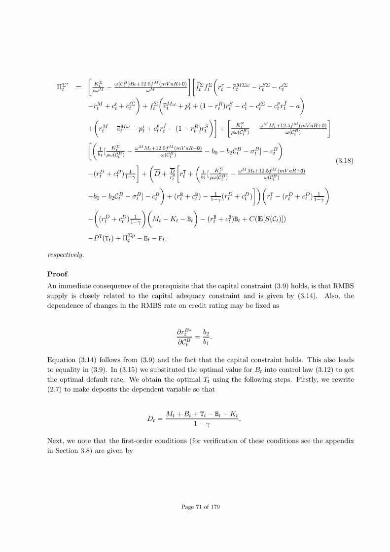
ΠΣ∗

t =

[KΣ

t

ρωM − ω(CBt )Bt+12.5fM (mV aR+O)

ωM

][fΣt f

Σt

(rrt − cMΣω


−rMt + ctt + ctΣt

)+ fΣ

t



ft − a

)

+

(rMt − cMω


St

)]+

[KΣ

t

ρω(CBt )

− ωMMt+12.5fM (mV aR+O)

ω(CBt )

]

[(1b1[

KΣt

ρω(CBt )


ω(CBt )

− b0 − b2CBt − σBt ]− cBt

)

−(rDt + cDt )1

1−γ

]+

(D + D

rpt

[rTt +

(1b1[

KΣt

ρω(CBt )


ω(CBt )

−b0 − b2CBt − σBt ]− cBt

)+ (rBt + cBt )− 1

1−γ (rDt + cDt )

])(rTt − (rDt + cDt )

11−γ

)

−((rDt + cDt )

11−γ

)(Mt −Kt − Bt

)− (rBt + cBt )Bt + C(E[S(Ct)])

−P T(Tt) + ΠΣpt − Et − Ft,

(3.18)

respectively.

Proof.

An immediate consequence of the prerequisite that the capital constraint (3.9) holds, is that RMBS

supply is closely related to the capital adequacy constraint and is given by (3.14). Also, the

dependence of changes in the RMBS rate on credit rating may be fixed as

∂rB∗t

∂CBt=

b2b1.

Equation (3.14) follows from (3.9) and the fact that the capital constraint holds. This also leads

to equality in (3.9). In (3.15) we substituted the optimal value for Bt into control law (3.12) to get

the optimal default rate. We obtain the optimal Tt using the following steps. Firstly, we rewrite

(2.7) to make deposits the dependent variable so that

Dt =Mt +Bt + Tt − Bt −Kt

1− γ.

Next, we note that the first-order conditions (for verification of these conditions see the appendix

in Section 3.8) are given by

Page 71 of 179

∂ΠΣt

∂rBt

[1 + cdwt −Et

{∫ B

B

δt,1∂V Σ

∂(KΣt+1)

dF (σBt+1)

}]− lbtρb1ω(CBt ) = 0; (3.19)

∂ΠΣt

∂Dt

[1 + cdwt −Et

{∫ B

B

δt,1∂V Σ

∂(KΣt+1)

dF (σBt+1)

}]= 0; (3.20)

ρ

[ω(CBt )Bt + ωMMt + 12.5fM (mV aR+ O)

]≤ KΣ

t ; (3.21)

−cdwt +Et

{∫ B

B

δt,1∂V Σ

∂(KΣt+1)

dF (σBt+1)

}= 0. (3.22)

Here F (·) is the cumulative distribution of the shock to the RMBS. Using (3.22) we can see that

(3.20) becomes

∂ΠΣt

∂Dt= 0.

Looking at the form of ΠΣt given in (3.2)and the equation

P T(Tt) =rpt2D

[D − Tt]2 (3.23)

it follows that

ΠΣt =

(rrt − cMΣω


)fΣt f

Σt Mt +


)(1− fΣ

t )fΣt Mt (3.24)

+

(rMt − cMω


St

)(1− fΣ

t )Mt − afΣt Mt + rTt Tt

+

(rBt − cBt

)Bt −

(rBt + cBt

)Bt −

(rDt + cDt

)Dt + C(E[S(Ct)])−

rpt2D

[D − Tt]2

+ΠΣpt − Et − Ft.

Finding the partial derivatives of SIB’s profit, ΠΣt , with respect to deposit, Dt, we have that

∂ΠΣt

∂Dt= (1− γ)

(rTt + (rBt + cBt ) + (rBt − cBt ) +

rptD(D − Tt)

)− (rDt + cDt ) (3.25)

This would then give us the optimal value for Dt. Using (2.7) and all the optimal values calculated

to date, we can find optimal deposits as well as optimal profits.

Page 72 of 179

The next corollary follows immediately from Theorem 3.2.4.

Corollary 3.2.5 (Solution to the Optimal Valuation Problem Under RMBSs (Slack)):

Suppose that JΣ and V Σ are given by (3.10) and (3.11), respectively and P (Ct) > 0. When the

capital constraint (3.9) does not hold (i.e., lbt = 0), a solution to the optimal valuation problem

under RMBSs stated in Problem 3.2.3 yields optimal RMBS supply and its rate

BΣn∗

t =2

3(b0 + b2CBt + σBt ) +

b13

[rMt − cMω

t − pit(Ct) + cpt rft + 2cBt (3.26)

−(1− rRt )rSt +

(rDt + cDt )

(1− γ)+

(rrt − cMΣω


)fΣt f

Σt

+

(cMωt + pit(Ct)− cpt r

ft + (1− rRt )r

St − ctt − ctΣt − a

)fΣt

]

and

rBΣn∗

t = − 1

3b1(b0 + b2CBt + σBt ) +

1

3

[rMt − cMω

t − pit(Ct) + cpt rft + 2cBt (3.27)

−(1− rRt )rSt +

(rDt + cDt )

(1− γ)+

(rrt − cMΣω


)fΣt f

Σt

+


ft + (1− rRt )r


)fΣt

],

respectively. In this case, the corresponding Tt, deposits and profits under RMBSs are given by

TΣn∗

t = D +D

rpt


1

1− γ(rDt + cDt )

](3.28)

DΣn∗

t =1

1− γ

(D +

D

rpt


1

1− γ(rDt + cDt )

](3.29)

+BΣn∗

t +Mt −Kt − Bt

)

and

Page 73 of 179

ΠΣn∗

t = Mt

[(rMt − c

Mωt − p

it(Ct) + c

pt r

ft − (1− r

Rt )r

St

)+

(rrt − c

MΣωt − r

SΣt − c

iΣt − r

Mt + c

t (3.30)

+ctΣt

)fΣt f

Σt +

(cMωt + p

it(Ct) + (1− r

Rt )r

St − c

t− c

tΣt − c

pt r

ft − a

)fΣt

]+

[2

3(b0 + b2C

Bt + σ

Bt )

+b1

3

(rMt − c

Mωt − p

it(Ct) + c

pt r

ft + 2cBt − (1− r

Rt )r

St +

(rDt + cDt )

(1− γ)+

(rrt − c

MΣωt − r

SΣt − c

iΣt

−rMt + c

tt + c

tΣt

)fΣt f

Σt +

(cMωt + p

it(Ct)− c

pt r

ft + (1− r

Rt )r

St − c

tt − c

tΣt − a

)fΣt

)]

{[1

3

(rMt − c

Mωt − p

it(Ct) + c

pt r

ft + 2cBt − (1− r

Rt )r

St +

(rDt + cDt )

(1− γ)+ (rrt − c

MΣωt − r

SΣt − c

iΣt

−rMt + c

tt + c

tΣt )fΣ

t fΣt + (cMω

t + pit(Ct)− c

pt r

ft + (1− r

Rt )r

St − c

tt − c

tΣt − a)fΣ

t

)

−1

3b1(b0 + b2C

Bt + σ

Bt )− c

Bt

]− (rDt + c

Dt )

1

1− γ

}+

(D +

D

rpt

[rT

t −

[1

3b1(b0 + b2C

Bt + σ

Bt )

−1

3

(rMt − c

Mωt − p

it(Ct) + c

pt r

ft + 2cBt − (1− r

Rt )r

St +

(rDt + cDt )

(1− γ)+ (rrt − c

MΣωt − r

SΣt − c

iΣt

−rMt + c

tt + c

tΣt )fΣ

t fΣt + (cMω

t + pit(Ct)− c

pt r

ft + (1− r

Rt )r

St − c

tt − c

tΣt − a)fΣ

t

)+ c

Bt

]

+(rBt + cB

t)−1

1− γ(rDt + c

Dt )

])(rT

t − (rDt + cDt )

1

1− γ

)−

((rDt + c

Dt )

1

1− γ

)(Mt −Kt − Bt

)

−(rBt + cB

t)Bt +C(E[S(Ct)])− PT(Tt) + ΠΣp

t − Et − Ft,

respectively.

Proof.

For the situation where capital constraint (3.9) does not hold (i.e., lbt = 0), using equation (3.22)

and the fact that lbt = 0, we can see that (3.19) becomes∂ΠΣ

t

∂rBt= 0. As in the proof of Theorem

3.2.4, looking at the form of ΠΣt given in (3.2) and (3.23), we have equation (3.24). Therefore

Page 74 of 179

∂ΠΣt

∂rBt= Bt − b1

[(rrt − cMΣω


)fΣt f

Σt (3.31)

+


ft + (1− rRt )r


)fΣt

+

(rMt − cMω


St

)]

+b1

[(rBt − cBt )− rTt − (rBt + cBt )

]− rpt

D(D − Tt)b1 = 0.

Substituting (3.25) into (3.31) and using (3.12) would give us optimal RMBSs and RMBS rate

given by (3.26) and (3.27), respectively. Furthermore we can find SIB’s optimal deposit, deposit

withdrawals and profits.

Further discussions of the key aspects of Section 3.2 is provided in Subsection 3.6.1.

3.3 Risk, Profit and Valuation Under RMBS CDOs

In this section, we discuss SIB’s risk, profit and valuation under RMBS CDOs. In the sequel, we

assume that the notation Π, rM , M, cMω, pi, cp, rf , rR, rS, S, C, C(E[S(C)]), rB, cB , B, rT, T,

P T(T), rD, cD, D, rB, cB, B, Πp, K, n, E, O, ω(C), ωB , fM , mV aR, O, rSΣ, fΣ and fΣ, corresponds

to that of Sections 2.3 and 3.2. Further suppositions about notation are that rr, cMΣω, ciΣ, ct, ctΣ,

a, ΠΣp, E and F denote the same parameters as in Section 3.2.

Assumption 3.3.1 (Senior Tranches of RMBSs): We assume that risky marketable securities,

B, appearing in the balance sheet (2.7), consist entirely of the senior tranches of RMBSs that are

wrapped by an MLI. Also, SIB has an incentive to retain an interest in these tranches.

This assumption implies that the CDO structure depends on the securitization of senior tranches

of RMBSs in particular.

3.3.1 Risk and Profit Under RMBS CDOs

In this subsection, we investigate a subprime mortgage model for profit under RMBS CDOs and

its relationship with retained earnings.

3.3.1.1 A Subprime Mortgage Model for Risk and Profit Under RMBS CDOs

In this thesis, a subprime mortgage model for profit under RMBS CDOs can be constructed by

considering the difference between cash inflow and outflow. For this profit, in period t, cash in-

flow is constituted by returns on the residual from RMBSs securitization, rrbt fΣbt fΣb

t Bt, securitized

subprime RMBSs, rBt (1− fΣbt )fΣb

t Bt, unsecuritized securities, rBt (1− fΣbt )Bt, Treasuries, r

T

t Tt, and

mortgages, rMt Mt, as well as the recovery amount, Rt, MLI protection leg payments, C(S(Ct)),

Page 75 of 179

and the present value of future gains from subsequent RMBS purchases and their securitizations,

ΠΣpt . On the other hand, we consider the average weighted cost of funds to securitize RMBSs,

cMΣωbfΣbt fΣb

t Bt, losses from securitized RMBSs, rSΣbt fΣbt fΣb

t Bt, forfeit costs related to MLI insur-

ance wrapping RMBS CDOs, ciΣbt fΣbt fΣb

t Bt, transaction cost to extend RMBSs, ctbt (1− fΣbt )fΣb

t Bt,

and transaction costs from securitized RMBSs ctΣbt (1−fΣbt )fΣb

t Bt as part of cash outflow. Additional

components of outflow are weighted average cost of funds for extending RMBSs, cMωbt (1− fΣb

t )Bt,

fraction of the face value of unsecuritized RMBSs corresponding to fΣbt (1− fΣb

t )Bt, MLI premium

for unsecuritized RMBSs losses, pibt (1− fΣbt )Bt, decreasing value of adverse selection, abfΣb

t Bt, the

all-in cost of holding RMBSs, cMt Mt, interest paid to depositors, rDt Dt, the cost of taking deposits,

cDDt, provisions against deposit withdrawals, P T(Tt), while rB and cB are the borrower rate and

marginal cost of borrowing, respectively, losses from suboptimal SPVs, Et and costs for funding

RMBS securitization, Ft. From the above, we have that model for profit under subprime RMBS

CDOs may have the form

ΠΣbt =

(rrt − cMΣω


)fΣt f

Σt Mt +


)(1− fΣ

t )fΣt Mt (3.32)

+

(rMt − cMω


St

)(1− fΣ

t )Mt − afΣt Mt

+

(rrbt − cMΣωb

t − rSΣbt − ciΣbt

)fΣbt fΣb

t Bt +

(rBt − ctbt − ctΣbt

)(1− fΣb

t )fΣbt Bt

+

(rBt − cMωb

t − pibt + cbpt rfbt − (1− rRbt )rSbt

)(1− fΣb

t )Bt − abfΣbt Bt + rTt Tt

−(rBt + cBt

)Bt −

(rDt + cDt

)Dt + C(E[S(Ct)])− P T(Tt) + ΠΣp

t − Et − Ft,

where ΠΣpt = Πpt + ΠΣ

t . Furthermore, by considering∂S(Ct)∂CBt

< 0 and (3.32), we know that ΠΣb is

an increasing function of current RMBS credit rating, CB .From the above, we note that in (3.32) the cash inflow terms rrbt fΣb

t fΣbt Bt and rBt (1 − fΣb

t )fΣbt Bt

carry credit, market (in particular, interest rate), tranching and operational risks while rBt (1 −fΣbt )Bt embed credit (in particular, counterparty) and market (in particular, interest rate) risks.

In (3.32), the cash outflow terms cMΣωbfΣbt fΣb

t Bt, rSΣbt fΣb

t fΣbt Bt, c

iΣbt fΣb

t fΣbt Bt, c

tbt (1− fΣb

t )fΣbt Bt

and ctΣbt (1−fΣbt )fΣb

t Bt involve credit (for instance, counterparty), market (specifically, liquidity and

valuation), tranching and operational risks. Also, cMωbt (1− fΣb

t )Bt and pibt (1− fΣbt )Bt carry credit,

market (particularly, liquidity) and operational risks while abfΣbt Bt embeds credit and market (in

the form of liquidity and valuation) risks. As before, the risks that we associate with each of the

cash inflow and outflow terms in (3.32) are less straightforward. For instance, strong correlations

may exist between each of the aforementioned risks. Also, the risk-carrying terms found in (3.32)

affect the entire banking system via systemic risk.

Page 76 of 179

3.3.1.2 Profit Under RMBS CDOs and Retained Earnings

We know that profits, Πt, are used to meet its obligations, that include dividend payments on

equity, ntdt. The retained earnings, Ert , subsequent to these payments may be computed by using

(3.3). After adding and subtracting

(rBt − cMωb

t − pibt + cpbt rfbt − (1 − rRbt )rSbt

)Bt from (3.32), we

get

ΠΣbt = Πt +

(rrt − cMΣω


)fΣt f

Σt Mt

+



ft − a

)fΣt Mt

+

(rrbt − cMΣωb

t − rSΣbt − ciΣbt − rBt + ctbt + ctΣbt

)fΣbt fΣb

t Bt

+

(cMωbt + pibt + (1− rRbt )rSbt − ctbt − ctΣbt − cpbt rfbt − ab

)fΣbt Bt

+

(rBt − cMωb

t − pibt + cpbt rfbt − (1− rRbt )rSbt

)Bt


Replace Πt by using (3.3). In this case ΠΣbt is given by

ΠΣbt = Er

t + ntdt + (1 + rOt )Ot +

(rrt − cMΣω

t − rSΣt − ciΣt − rMt + ctt (3.33)

+ctΣt

)fΣt f

Σt Mt +



ft − a

)fΣt Mt

+

(rrbt − cMΣωb


)fΣbt fΣb

t Bt

+


)fΣbt Bt

+

(rBt − cMωb


)Bt


For (3.33) and (2.10) to obtain an expression for capital of the form

Page 77 of 179

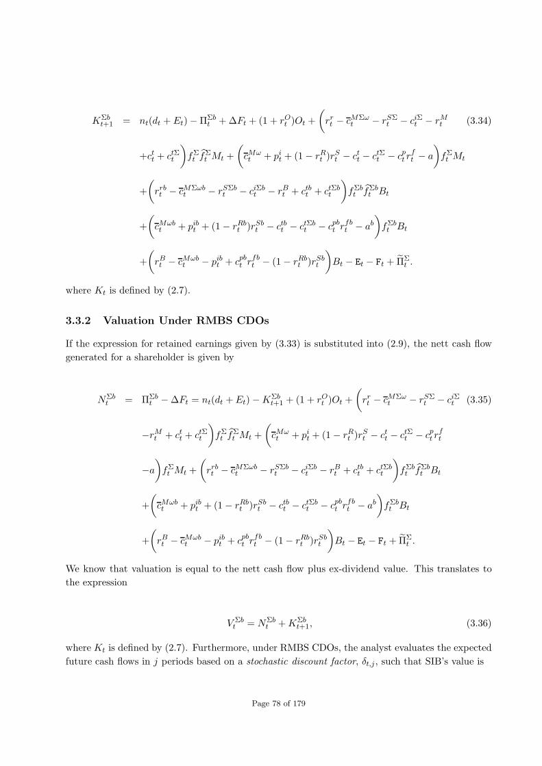
KΣbt+1 = nt(dt + Et)−ΠΣb

t +∆Ft + (1 + rOt )Ot +

(rrt − cMΣω

t − rSΣt − ciΣt − rMt (3.34)

+ctt + ctΣt

)fΣt f

Σt Mt +



ft − a

)fΣt Mt

+

(rrbt − cMΣωb


)fΣbt fΣb

t Bt

+


)fΣbt Bt

+

(rBt − cMωb


)Bt − Et − Ft + ΠΣ

t .

where Kt is defined by (2.7).

3.3.2 Valuation Under RMBS CDOs

If the expression for retained earnings given by (3.33) is substituted into (2.9), the nett cash flow

generated for a shareholder is given by

NΣbt = ΠΣb

t −∆Ft = nt(dt +Et)−KΣbt+1 + (1 + rOt )Ot +

(rrt − cMΣω

t − rSΣt − ciΣt (3.35)


)fΣt f

Σt Mt +



ft

−a

)fΣt Mt +

(rrbt − cMΣωb


)fΣbt fΣb

t Bt

+


)fΣbt Bt

+

(rBt − cMωb


)Bt − Et − Ft + ΠΣ

t .

We know that valuation is equal to the nett cash flow plus ex-dividend value. This translates to

the expression

V Σbt = NΣb

t +KΣbt+1, (3.36)

where Kt is defined by (2.7). Furthermore, under RMBS CDOs, the analyst evaluates the expected

future cash flows in j periods based on a stochastic discount factor, δt,j , such that SIB’s value is

Page 78 of 179

V Σbt = NΣb

t +Et

[ ∞∑

j=1

δt,jNΣbt+j

]. (3.37)

3.3.3 Optimal Valuation Under RMBS CDOs

In this subsection, we make use of the modeling of assets, liabilities and capital of the preceding

section to solve an optimal valuation problem.

3.3.3.1 Statement of Optimal Valuation Problem Under RMBS CDOs

Suppose that SIB’s valuation performance criterion, JΣb, at t is given by

JΣbt = ΠΣb

t + lbt

[KΣbt − ρ

(ωMMt + ω(CBt )Bt + 12.5fM (mV aR+ O)

)](3.38)

−cdwt

[KΣbt+1

]+Et

[δt,1V

(KΣbt+1, xt+1

)],

where lbt is the Lagrangian multiplier for the total capital constraint, KΣt is defined by (3.9), Et[·]

is the expectation conditional on SIB’s information in period t and xt is the deposit withdrawls in

period t with probability distribution f(xt). Also, cdwt is the deadweight cost of total capital that

consists of equity.

The optimal valuation problem is to maximize the value given by (3.37). We can now state the

optimal valuation problem as follows.

Problem 3.3.2 (Statement of Optimal Valuation Problem Under RMBS CDOs): Sup-

pose that the total capital constraint, KΣb, and the performance criterion, JΣb, are given by (3.9)

and (3.38), respectively. SIB’s optimal valuation problem is to maximize its value given by (3.37)

by choosing the RMBS rate, deposits and regulatory capital for

V Σb(KΣbt , xt) = max

rBt , Dt, ΠΣbt

JΣbt , (3.39)

subject to RMBS, balance sheet, cash flow and financing constraints given by (3.12), (3.13), (3.32)

and (3.34), respectively.

3.3.3.2 Solution of Optimal Valuation Problem Under RMBS CDOs

In this subsection, we find a solution to Problem 3.3.2 when the capital constraint (3.9) holds as

well as when it does not. In this regard, the main result can be stated and proved as follows.

Page 79 of 179

Theorem 3.3.3 (Solution to an Optimal Valuation Problem Under RMBS CDOs): Sup-

pose that JΣb and V Σb are given by (3.38) and (3.39), respectively. When the capital constraint

given by (3.9) holds (i.e., lbt > 0), a solution to the optimal valuation problem yields an optimal

RMBS supply and rate given by (3.14) and (3.15), respectively. In this case, optimal deposits,

provisions for deposit withdrawals via Treasuries and profits under RMBS CDO securitization are

given by

DΣb∗t =

1

1− γ

(D +

D

rpt

[rTt + (rBt + cBt )−

1

1− γ(rDt + cDt )

](3.40)

+KΣbt

ρω(CBt )− ωMMt + 12.5fB(mV aR+ O)

ω(CBt )+Mt −Kt − Bt

),

TΣb∗

t = D +D

rpt


1

1− γ(rDt + cDt )

](3.41)

and

Page 80 of 179

ΠΣb∗

t =

[KΣbt

ρωM− ω(CBt )Bt + 12.5fM (mV aR+ O)

ωM

][fΣt f

Σt

(rrt − cMΣω

t − rSΣt − ciΣt (3.42)


)+ fΣ

t



ft − a

)

+

(rMt − cMω


St

)]+

[KΣbt

ρω(CBt )

−ωMMt + 12.5fM (mV aR+ O)

ω(CBt )

][fΣbt fΣb

t

(rrbt − cMΣωb


+1

b1

(b0 −

KΣbt

ρω(CBt )+

ωMMt + 12.5fM (mV aR+ O)

ω(CBt )+ b2CBt + σBt

)+ ctbt + ctΣbt

)

+fΣbt


)

−(

1

b1

(b0 −

KΣbt

ρω(CBt )+


ω(CBt )+ b2CBt + σBt

)

+cMωbt + pibt − cpbt rfbt + (1− rRbt )rSbt

)− (rDt + cDt )

1

1− γ

]

+

(D +

D

rpt


1

1− γ(rDt + cDt )

])


1

1− γ

)−((rDt + cDt )

1

1− γ

)(Mt −Kt − Bt

)

−(rBt + cBt )Bt + C(E[S(Ct)])− P T(Tt) + ΠΣpt − Et − Ft,

respectively.

Proof. A complete proof is provided in Subsection 3.8.2 of Section 3.8.

The next corollary follows immediately from Theorem 3.3.3.

Corollary 3.3.4 (Solution to the Optimal Valuation Problem Under RMBS CDOs

(Slack)): Suppose that JΣb and V Σb are given by (3.38) and (3.39), respectively and P (Ct) > 0.

When the capital constraint (3.9) does not hold (i.e., lbt = 0), a solution to the optimal valuation

problem under RMBS CDOs stated in Problem 3.3.2 yields optimal RMBS CDO supply and its rate

Page 81 of 179

BΣbn∗

t =1

2(b0 + b2CBt + σBt ) +

b1

2(1 − fΣbt fΣb

t )

[cMΣωbt + pibt + (1− rRbt )rSbt (3.43)

−cpbt rfbt +(rDt + cDt )

2(1 − γ)−(rrbt − cMΣωb

t − rSΣbt − ciΣbt + ctbt + ctΣbt

)fΣbt fΣb

t

−(cMωbt + pibt + (1− rRbt )rSbt − ctbt − ctΣbt − cpbt rfbt − ab

)fΣbt

]

and

rBΣbn∗

t = − 1

2b1(b0 + b2CBt + σBt ) +

1

2(1 − fΣbt fΣb

t )

[cMΣωbt + pibt + (1− rRbt )rSbt (3.44)




)fΣbt fΣb

t


)fΣbt

],

respectively. In this case, the corresponding Tt, deposits and profits under RMBS CDOs are given

by

TΣbn∗

t = D +D

rpt


1

1− γ(rDt + cDt )

](3.45)

DΣbn∗

t =1

1− γ

(D +

D

rpt


1

1− γ(rDt + cDt )

](3.46)

+BΣbn∗

t +Mt −Kt − Bt

).

and

Page 82 of 179

ΠΣbn∗

t = Mt

[(rrt − cMΣω


)fΣt f

Σt +

(cMωt + pit (3.47)

+(1− rRt )rSt − ctt − ctΣt − cpt r

ft − a

)fΣt +

(rMt − cMω


St

)]

+

[1

2(b0 + b2CBt + σBt ) +

b1

2(1 − fΣbt fΣb

t )

(cMΣωbt + pibt + (1− rRbt )rSbt − cpbt rfbt

+(rDt + cDt )

2(1− γ)−(rrbt − cMΣωb


)fΣbt fΣb

t −(cMωbt + pibt

+(1− rRbt )rSbt − ctbt − ctΣbt − cpbt rfbt − ab)fΣbt

)]{fΣbt fΣb

t

(rrbt − cMΣωb

t − rSΣbt

−ciΣbt +

[1

2b1(b0 + b2CBt + σBt )−

1

2(1 − fΣbt fΣb

t )

(cMΣωbt + pibt + (1− rRbt )rSbt




)fΣbt fΣb

t


)fΣbt

)]+ ctbt + ctΣbt

)

+fΣbt


)

−([

1

2b1(b0 + b2CBt + σBt )−

1

2(1 − fΣbt fΣb

t )

(cMΣωbt + pibt + (1− rRbt )rSbt




)fΣbt fΣb

t


)fΣbt

)]

+cMωbt + pibt − cpbt rfbt + (1− rRbt )rSbt

)− (rDt + cDt )

1

1− γ

}

+

(D +

D

rpt


1

1− γ(rDt + cDt )

])


1

1− γ

)−((rDt + cDt )

1

1− γ

)(Mt −Kt − Bt

)

−(rBt + cBt )Bt + C(E[S(Ct)])− P T(Tt) + ΠΣpt − Et − Ft,

Further discussion of important issues raised in Section 3.3 is provided in Subsection 3.6.2.

Page 83 of 179

3.4 Mortgage Securitization and Capital Under Basel Regulation

In this section, we deal with a model where both subprime RMBS default and risk-weights are

a function of the current level of credit rating, CBt . The capital constraint is described by the

expression in (2.13), where the risk-weights on RMBSs, ωB 6= 0, are considered. Also, in this

situation, the risk-weight on RMBSs, ω(CBt ), is a decreasing function of the current level of credit

rating, i.e,∂ω(CBt )∂CBt

< 0. In particular, the risk-weights for mortgages are kept constant, i.e., ωM = 1.

In this case, the capital constraint (2.13) becomes

Kt ≥ ρ

[ωMMt + ω(CBt )Bt + 12.5fM (mV aR+ O)

]. (3.48)

3.4.1 Quantity and Pricing of RMBSs, RMBS CDOs and Capital Under Basel

Regulation (Securitized Case)

In this subsection, we firstly examine how capital, K, and the quantity and price of RMBSs, B,

are affected by changes in the level of credit rating, CB , when risk-weight on RMBSs, ω(CBt ), areallowed to vary as in Section 3.2. Secondly, we will provide an analogue of this result for RMBS

CDOs.

Theorem 3.4.1 (Mortgage Securitization and Capital under Basel Regulation (Secu-

ritized Case)): Suppose that the assumptions in Section 3.2 hold and that B(CBt ) > 0 and the

RMBS risk-weight, ω(CBt ), are allowed to vary. In this case, we have that

1. if∂σB

∗

t+1

∂CBt< 0 then

∂KΣt+1

∂CBt> 0;

2. if∂σB

∗

t+1

∂CBt> 0 then

∂KΣt+1

∂CBt< 0.

Proof.

We equate SIB’s optimal RMBSs for the problems with lbt = 0 and lbt > 0 in order to obtain

2

3(b0 + b2CBt + σBt ) +

b13

[rMt − cMω

t − pit(Ct) + cpt rft + 2cBt − (1− rRt )r

St +

(rDt + cDt )

(1− γ)

+

(rrt − cMΣω


)fΣt f

Σt +


ft

+(1− rRt )rSt − ctt − ctΣt − a

)fΣt

]=

KΣt

ρω(CBt )− Mt + 12.5fM (mV aR+ O)

ω(CBt ).

Solving for σBt , we obtain

Page 84 of 179

σB∗

t = 3

(KΣt


ω(CBt )

)− 2(b0 + b2CBt )− b1

[rMt − cMω

t − pit(Ct)

+cpt rft + 2cBt − (1− rRt )r

St +

(rDt + cDt )

(1− γ)+

(rrt − cMΣω


)fΣt f

Σt

+


ft + (1− rRt )r


)fΣt

]

Using equation (3.19) and substituting equation (3.17), we obtain

b1ρω(CBt )lbt = b1

[2(rBt − cBt )−

(rrt − cMΣω


)fΣt f

Σt

−(cMωt + pit(Ct)− cpt r

ft + (1− rRt )r


)fΣt

−(rMt − cMω


St

)− (rDt + cDt )

1− γ

]+B∗

t .

Substitute rB∗

t and B∗t into the expression above to obtain

lb∗

t =2σBt − σB

∗

t

ω(CBt )ρb1.

Using equation (3.11) to find the partial derivative of the value function with respect to SIB capital

we obtain

∂V Σ

∂KΣt

=

lbt +1

1− γ(rDt + cDt ),

1

1− γ(rDt + cDt ), for B ≤ σBt ≤ σB

∗

t ,

1

1− γ(rDt + cDt ) +

2σBt − σB∗

t

ω(CBt )ρb1, for σB

∗

t ≤ σBt ≤ B.

By substituting the above expression into the optimal condition for total capital (3.22), we obtain

cdwt −Et

[δt,1

1

1− γ(rDt + cDt )

]− 1

ω(CBt+1)ρb1Et

[ ∫ B

σB∗

t+1

δt,1

(2σBt+1 − σB

∗

t+1

)dF (σBt+1)

]= 0.

We denote the left-hand side of the above expression by Y, so that

Page 85 of 179

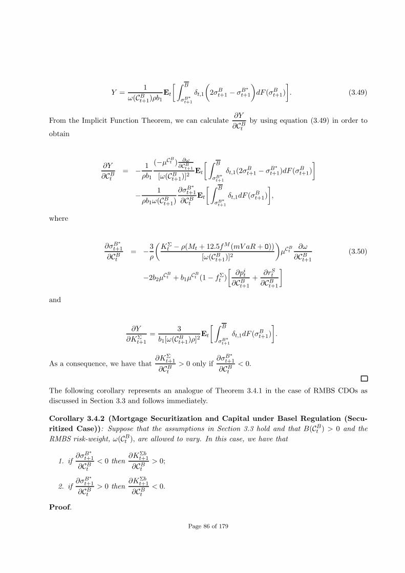
Y =1

ω(CBt+1)ρb1Et

[ ∫ B

σB∗

t+1

δt,1

(2σBt+1 − σB

∗

t+1

)dF (σBt+1)

]. (3.49)

From the Implicit Function Theorem, we can calculate∂Y

∂CBtby using equation (3.49) in order to

obtain

∂Y

∂CBt= − 1

ρb1

(−µCBt ) ∂ω

∂CBt+1

[ω(CBt+1)]2

Et

[ ∫ B

σB∗

t+1

δt,1(2σBt+1 − σB

∗

t+1)dF (σBt+1)

]

− 1

ρb1ω(CBt+1)

∂σB∗

t+1

∂CBtEt

[ ∫ B

σB∗

t+1

δt,1dF (σBt+1)

],

where

∂σB∗

t+1

∂CBt= −3

ρ

(KΣt − ρ(Mt + 12.5fM (mV aR+ O))

[ω(CBt+1)]2

)µCB

t∂ω

∂CBt+1

(3.50)

−2b2µCBt + b1µ

CBt (1− fΣ

t )

[∂pit

∂CBt+1

+∂rSt∂CBt+1

]

and

∂Y

∂KΣt+1

=3

b1[ω(CBt+1)ρ]2Et

[ ∫ B

σB∗

t+1

δt,1dF (σBt+1)

].

As a consequence, we have that∂KΣ

t+1

∂CBt> 0 only if

∂σB∗

t+1

∂CBt< 0.

The following corollary represents an analogue of Theorem 3.4.1 in the case of RMBS CDOs as

discussed in Section 3.3 and follows immediately.

Corollary 3.4.2 (Mortgage Securitization and Capital under Basel Regulation (Secu-

ritized Case)): Suppose that the assumptions in Section 3.3 hold and that B(CBt ) > 0 and the

RMBS risk-weight, ω(CBt ), are allowed to vary. In this case, we have that

1. if∂σB

∗

t+1

∂CBt< 0 then

∂KΣbt+1

∂CBt> 0;

2. if∂σB

∗

t+1

∂CBt> 0 then

∂KΣbt+1

∂CBt< 0.

Proof.

Page 86 of 179

We equate SIB’s optimal RMBS CDOs for the problems with lbt = 0 and lbt > 0 in order to obtain

1

2(b0 + b2CBt + σBt ) +

b1

2(1 − fΣbt fΣb

t )

[cMΣωbt + pibt + (1− rRbt )rSbt − cpbt rfbt +

(rDt + cDt )

2(1− γ)

−(rrbt − cMΣωb


)fΣbt fΣb

t −(cMωbt + pibt + (1− rRbt )rSbt

−ctbt − ctΣbt − cpbt rfbt − ab)fΣbt

]=

KΣbt


ω(CBt ).

Solving for σBt , we obtain

σB∗

t = 2(1 − fΣbt fΣb

t )

(KΣbt


ω(CBt )

)− (1− fΣb

t fΣbt )(b0 + b2CBt )

−b1

[cMΣωbt + pibt + (1− rRbt )rSbt − cpbt rfbt +

(rDt + cDt )



+ctbt + ctΣbt

)fΣbt fΣb

t −(cMωbt + pibt + (1− rRbt )rSbt − ctbt − ctΣbt − cpbt rfbt − ab

)fΣbt

]

Using equation (3.61) and substituting equation (3.41), we obtain

b1ρω(CBt )lbt = 2b1

[(rBt − cMωb


)+

(rrbt − cMΣωb

t

−rSΣbt − ciΣbt − rBt + ctbt + ctΣbt

)fΣbt fΣb

t +

(cMωbt + pibt + (1− rRbt )rSbt

−ctbt − ctΣbt − cpbt rfbt − ab)fΣbt − (rDt + cDt )

2(1− γ)

]+ 2(1− fΣb

t fΣbt )B∗

t .

Substitute rB∗

t and B∗t into the expression above to obtain

lb∗

t =σBt − σB

∗

t

ω(CBt )ρb1.

Using equation (3.39) to find the partial derivative of the value function with respect to SIB capital

we obtain

Page 87 of 179

∂V Σb

∂KΣbt

=

lbt +1

1− γ(rDt + cDt ),

1

1− γ(rDt + cDt ), for B ≤ σBt ≤ σB

∗

t ,

1

1− γ(rDt + cDt ) +

σBt − σB∗

t

ω(CBt )ρb1, for σB

∗

t ≤ σBt ≤ B.

By substituting the above expression into the optimal condition for total capital (3.64), we obtain

cdwt −Et

[δt,1

1

1− γ(rDt + cDt )

]− 1

ω(CBt+1)ρb1Et

[ ∫ B

σB∗

t+1

δt,1

(σBt+1 − σB

∗

t+1

)dF (σBt+1)

]= 0.

We denote the left-hand side of the above expression by Y, so that

Y =1

ω(CBt+1)ρb1Et

[ ∫ B

σB∗

t+1

δt,1

(σBt+1 − σB

∗

t+1

)dF (σBt+1)

]. (3.51)

From the Implicit Function Theorem, we can calculate∂Y

∂CBtby using equation (3.51) in order to

obtain

∂Y

∂CBt= − 1

ρb1

(−µCBt ) ∂ω

∂CBt+1

[ω(CBt+1)]2

Et

[ ∫ B

σB∗

t+1

δt,1(σBt+1 − σB

∗

t+1)dF (σBt+1)

]

− 1

ρb1ω(CBt+1)

∂σB∗

t+1

∂CBtEt

[ ∫ B

σB∗

t+1

δt,1dF (σBt+1)

],

where

∂σB∗

t+1

∂CBt= −2

ρ

(KΣbt − ρ(Mt + 12.5fM (mV aR+ O))

[ω(CBt+1)]2

)µCB

t∂ω

∂CBt+1

(3.52)

−b2µCBt − b1µ

CBt (1− fΣb

t )

[∂pibt∂CBt+1

+∂rSbt∂CBt+1

]

and

∂Y

∂KΣbt+1

=2

b1[ω(CBt+1)ρ]2Et

[ ∫ B

σB∗

t+1

δt,1dF (σBt+1)

].

Page 88 of 179

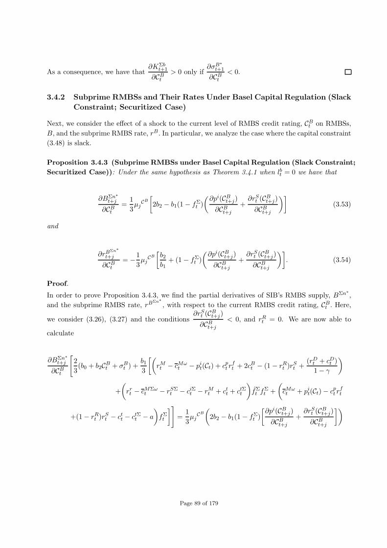
As a consequence, we have that∂KΣb

t+1

∂CBt> 0 only if

∂σB∗

t+1

∂CBt< 0.

3.4.2 Subprime RMBSs and Their Rates Under Basel Capital Regulation (Slack

Constraint; Securitized Case)

Next, we consider the effect of a shock to the current level of RMBS credit rating, CBt on RMBSs,

B, and the subprime RMBS rate, rB . In particular, we analyze the case where the capital constraint

(3.48) is slack.

Proposition 3.4.3 (Subprime RMBSs under Basel Capital Regulation (Slack Constraint;

Securitized Case)): Under the same hypothesis as Theorem 3.4.1 when lbt = 0 we have that

∂BΣn∗

t+j

∂CBt=

1

3µj

CB

[2b2 − b1(1− fΣ

t )

(∂pi(CBt+j)∂CBt+j

+∂rSt (CBt+j)∂CBt+j

)](3.53)

and

∂rBΣn∗

t+j

∂CBt= −1

3µj

CB

[b2b1

+ (1− fΣt )

(∂pi(CBt+j)∂CBt+j


)]. (3.54)

Proof.

In order to prove Proposition 3.4.3, we find the partial derivatives of SIB’s RMBS supply, BΣn∗

,

and the subprime RMBS rate, rBΣn∗

, with respect to the current RMBS credit rating, CBt . Here,

we consider (3.26), (3.27) and the conditions∂rSt (CBt+j)∂CBt+j

< 0, and rRt = 0. We are now able to

calculate

∂BΣn∗

t+j

∂CBt

[2

3(b0 + b2CBt + σBt ) +

b13

[(rMt − cMω


St +

(rDt + cDt )

1− γ

)

+

(rrt − cMΣω


)fΣt f

Σt +


ft


)fΣt

]]=

1

3µj

CB

(2b2 − b1(1− fΣ

t )

[∂pi(CBt+j)∂CBt+j


])

Page 89 of 179

and

∂rBΣn∗

t+j

∂CBt

[− 1

3b1(b0 + b2CBt + σBt ) +

1

3

[(rMt − cMω


St

+(rDt + cDt )

1− γ

)+

(rrt − cMΣω


)fΣt f

Σt +


ft


)fΣt

]]= −1

3µj

CB

(b2b1

+ (1− fΣt )

[∂pi(CBt+j)∂CBt+j


]).

3.4.3 Subprime RMBSs and Their Rates Under Basel Capital Regulation (Hold-

ing Constraint; Securitized Case)

Next, we present results about the effect of changes in the level of credit rating, CB , on RMBSs

when the capital constraint (3.48) holds.

Proposition 3.4.4 (Subprime RMBSs under Basel Capital Regulation (Holding Con-

straint; Securitized Case)): Assume that the same hypothesis as in Theorem 3.4.1 holds. If

lbt > 0 then by taking the first derivatives of equation (3.14) with respect to CBt and using the fact

that the risk-weights for mortgages, ωM , are constant we obtain

∂B∗t

∂CBt= −

KΣt − ρ

(ωMMt + 12.5fM (mV aR+ O)

)

[ω(CBt )]2ρ∂ω(CBt )∂CBt

. (3.55)

In this situation, the subprime RMBS payout rate response to changes in the level of credit rating

is given by

∂rB∗

t

∂CBt= −b2

b1−

KΣt − ρ

(ωMMt + 12.5fM (mV aR+ O)

)

[ω(CBt )]2ρb1∂ω(CBt )∂CBt

. (3.56)

Proof.

In order to prove Proposition 3.4.4, we find the partial derivatives of the optimal RMBS supply,

B∗, and subprime RMBS rate, rB, with respect to CBt . This involves using the equations (3.14) and

(3.15) and the condition∂ω(CBt+j)∂CBt+j

< 0 in order to find∂B∗

t

∂CBtand

∂rB∗

t

∂CBt, respectively. We are now

able to determine that

Page 90 of 179

∂B∗t

∂CBt

(KΣt

ρω(CBt )−[ωMMt + 12.5fM (mV aR+ O)

ω(CBt )

])

= −KΣt − ρ(12.5fM (mV aR+ O) + ωMMt)

[ω(CBt )]2ρ∂ω(CBt )∂CBt

and

∂rB∗

t

∂CBt

(− 1

b1

(b0 + b2CBt + σBt − KΣ

t

ρω(CBt )+


ω(CBt )

))

= −b2b1

− KΣt − ρ(12.5fM (mV aR+ O) + ωMMt)

[ω(CBt )]2ρb1∂ω(CBt )∂CBt

as required to complete the proof of Proposition 3.4.4.

3.4.4 Subprime RMBSs and Their Rates Under Basel Capital Regulation (Fu-

ture Time Periods; Securitized Case)

In the sequel, we examine the effect of a current credit rating shock in future periods on subprime

RMBSs, B, and their payout rates, rB. If the capital constraint is slack, the response of subprime

RMBSs and their rates in period j ≥ 1 to current fluctuations in the level of credit rating is

described by Theorem 3.4.1. Nevertheless, as time goes by, the impact of the credit rating shock

is minimized since µCB

j < 1. In future, if the capital constraint holds, the response of subprime

RMBSs and their rates to a change in the level of credit rating, CBt , is described by

∂B∗t+j

∂CBt=

µCB

j−1

ω(CBt+j)ρ

[∂(KΣ

t+j − ρ(ωMMt+j + 12.5fM (mV aR+ O)))

∂CBt−1+j

](3.57)

−µCB

j−1

ω(CBt+j)ρ

[µCB

ω(CBt+j)(KΣ

t+j − ρ(ωMMt+j + 12.5fM (mV aR+ O)))∂ω(CBt+j)∂CBt+j

]

and

∂rB∗

t+j

∂CBt= −b2

b1µCB

j +µCB

j−1

ω(CBt+j)ρb1∂(KΣ

t+j − ρ(ωMMt+j + 12.5fM (mV aR+ O)))

∂CBt−1+j

−µCB

j

[ω(CBt+j)]2ρ(KΣ

t+j − ρ(ωMMt+j + 12.5fM (mV aR+ O)))∂ω(CBt+j)∂CBt+j

.

From the equation (3.57), it can be seen that future subprime RMBSs can either rise or fall in

response to positive credit rating shocks. This process depends on the relative magnitudes of the

terms in equation (3.57). If capital rises in response to positive credit rating shocks, subprime

Page 91 of 179

RMBSs can fall provided that the effect of the shock on capital is greater than the effect of the

shock on subprime RMBS risk-weights.

Further discussions on important issues emphasized in Section 3.4 is given in Subsection 3.6.3.

3.5 Examples Involving Subprime Mortgage Securitization

In this section, we provide examples to illustrate some of the results obtained in the preceding

sections. In one way or the other all of the examples in this section support the claim that the

SMC was mainly caused by the intricacy and design (refer to Subsections 3.5.1, 3.5.3 and 3.5.4)

of systemic agents (refer to Subsection 3.5.1), subprime mortgage origination (refer to Subsections

3.5.3 and 3.5.4) and securitization (refer to Subsections 3.5.1, 3.5.3 and 3.5.4) that led to information

(loss, asymmetry and contagion) problems, valuation opaqueness and ineffective risk mitigation

(refer to Subsections 3.5.1, 3.5.3 and 3.5.4).

3.5.1 Numerical Example Involving Subprime Mortgage Securitization

In this subsection, we present a numerical example to highlight some issues in Sections 3.2 and 3.3.

In particular, we address the role of valuation in house prices. Here we bear in mind that we solve

a subprime mortgage securitization maximization problem subject to the financing and regulatory

capital constraints, with and without CDO tranching.

The choices of the values of the economic variables in this subsection are justified by considering

data from LoanPerformance (LP), Bloomberg, ABSNET, Federal Housing Finance Agency (FHFA;

formerly known as OFHEO), Federal Reserve Bank of St Louis (FRBSL) database, Financial Ser-

vice Research Program’s (FSRP) subprime mortgage database, Securities Industry and Financial

Markets Association (SIFMA) Research and Statistics as well as Lender Processing Services (LPS;

formerly called McDash Analytical) for selected periods before and during the crisis. Additional pa-

rameter choices are made by looking at, for instance, [7] and [53]. These provide enough information

to support the choices for prices, rates and costs while the parameter amounts are arbitrary.

3.5.1.1 Choices of Subprime Mortgage Securitization Parameters

In Table 3.2 below, we make choices for subprime securitization, profit and valuation parameters.

Page 92 of 179

Parameter Period t Period t + 1 Parameter Period t Period t + 1 Parameter Period t Period t + 1

M $ 10 000 $ 12 000 m0 $ 5 000 $ 5 000 L 0.909 1.043

ωM 0.05 0.05 m1 $ 5 000 $ 5 000 L1∗ 0.9182 1.0554

rM 0.051 0.082 m2 $ 5 000 $ 5 000 Ln∗ 0.3802 0.4439

cMω 0.0414 0.0414 CB 0.5 0.5 L2∗ 0.9201 1.0563

pi 0.01 0.01 a 0.05 0.05 cp∗ 0.0611 0.0633

cp 0.05 0.05 C(E[S(Ct)]) 400 400 ∆F 2 062.3 –

rf 0.01 0.01 rp 0.1 0.1 b0 $ 5 000 $ 5 000

rR 0.5 0.5 K $ 500 $ 650 b1 $ 5 000 $ 5 000

rS 0.15 0.25 O $ 150 $ 150 b2 $ 5 000 $ 5 000

H $ 11 000 $ 11 500 rO 0.101 0.101 ciΣ 0.05 0.06

Λ $ 50 000 $ 63 157.89 E $ 250 $ 250 cMΣω 0.045 0.045

ρ 0.08 0.08 Ep $ 150 $ 150 ct 0.03 0.03

C $ 1 000 $ 1 000 Ec $ 100 $ 100 ctΣ 0.04 0.04

rB 0.105 0.105 rB 0.1 0.1 rr 0.041 0.072

cB 0.101 0.101 cB 0.09 0.09 rSΣ 0.15 0.25

B $ 1 300 $ 1 500 B $ 5 200 $ 6 200 fΣ 0.3 0.2

ωB 0.5 0.5 Πp $ 6 000 $ 6 000 fΣ 0.65 0.5

rT 0.036 0.04 D $ 9 300 $ 11 100 F 700 500

T $ 2 000 $ 2 000 rD 0.105 0.105 E 500 300

O 150 150 rO 0.101 0.101 ab 0.05 0.05

n 1.75 2 rL 0.02 0.05 ΠΣp $ 8 000 $ 8 000

d 5.4 5.4 fM 0.08 0.19 ΠΣ 2 000 2 000

mV ar 400 400 ω(CB) 0.5 0.5 rrb 0.041 0.072

P T $ 800 $ 1 200 cD 0.101 0.101 cMΣωb 0.05 0.05

γ 0.1828 0.2207 0.031 0.032 ciΣ 0.05 0.06

S 750 1 500 R 550 575 rSΣb 0.15 0.25

Er $ 1 849.8 $ 518.65 σM 2 755 4 910 ctb 0.035 0.035

u 0.03621 0.06587 v 0.90329 0.90329 ctΣb 0.045 0.045

w 0.04429 0.04398 Π $ 2 024.4 $ 694.6 fΣb 0.4 0.3

M∗ $ 10 100 $ 12 137.5 rM∗

0.031 0.0545 fΣb 0.2 0.15

D∗ $ 15 387.34 $ 18 631.82 T∗ $ 7 246.53 $ 7 732.28 pib 0.01 0.01

Π∗ $ 656.02 - $ 974.36 Mn∗$ 4 182.55 $ 5 104.4 rRb 0.5 0.5

rMn∗

0.8365 1.0209 Tn∗$ 7 246.53 $ 7 732.28 rSb 0.15 0.25

Dn∗$ 8 601.42 $ 9 606.93 Πn∗

$ 7 659.27 $ 8 918.64 cpb 0.05 0.05

rfb 0.01 0.01 fB 0.08 0.08 ciΣb 0.05 0.06

cMωb 0.05 0.055 cM 0.04 0.06 rpΣ 0.01 0.01

Table 3.2: Choices of Capital, Information, Risk and Valuation Parameters Under Securitization

3.5.1.2 Computation of Subprime Mortgage Securitization Parameters

We compute important equations by using the values from Table 3.2. For Et−1 = (500−150)/1.75 =

200 and Et = (650 − 150)/2 = 250, in period t, SIB’s profit under RMBSs and retained earnings

in (3.4) is given by ΠΣt = 2502. SIB’s capital in (3.5) is given by KΣ

t+1 = 650 while the nett cash

flow under RMBSs given by (3.6) is computed as NΣt = 439.7. Furthermore, valuation in (3.7) is

equal to V Σt = 1089.7, while total capital constraint in (3.9) is given by KΣ

t = 500 ≥ 136. SIB’s

optimal valuation problem under RMBSs is to maximize the value by choosing the RMBS rate,

deposits and regulatory capital for (3.11) subject to RMBS, balance sheet, cash flow and financing

constraints given by (3.12), (3.13), (3.2) and (3.5), respectively. Here, we have σBt = −6725 and

Dt = 9300. SIB’s optimal RMBS supply (3.14) and its rate (3.15) are given by B∗t = 10400 and

rB∗

t = 1.925, respectively. In this case, optimal deposits (3.16), provisions for deposit withdrawals

via Treasuries (3.17) and profits under RMBS securitization (3.18) are given by DΣ∗

t = 26855.77,

TΣ∗

t = 7246.53 and ΠΣ∗

t = −28284.7, respectively.

When the capital constraint (3.9) does not hold, then the solutions for SIB’s optimal RMBSs

Page 93 of 179

(3.26) and RMBS rate (3.27) are given by BΣn∗

t = 1094.9 and rBΣn∗

t = 0.064, respectively. In this

case, corresponding optimal deposits (3.29) and profits (3.30) are given by DΣn∗

t = 15469.2 and

ΠΣn∗

t = 2198.6, respectively.

The following values are computed in period t under RMBS CDOs. SIB’s profit under RMBS CDOs

and retained earnings in (3.33) is given by ΠΣbt = 2463.5, while SIB’s capital in (3.34) is given by

KΣbt+1 = 650. SIB’s nett cash flow (3.35) for a shareholder is given by NΣb

t = 401.2 Furthemore SIB’s

valuation in (3.36) is equal to V Σbt = 1051.2 respectively. Optimal deposits (3.40), provisions for

deposit withdrawals via Treasuries (3.41) and profits under RMBS CDO securitization (3.42) are

given by DΣb∗t = 26400.56, TΣb

∗

t = 6874.53 and ΠΣb∗t = 6330.82,. If capital constraint (3.9) does not

hold, then SIB’s optimal RMBS CDO supply (3.43) and rate (3.44) are given by BΣbn∗

t = 1118.64

and rBΣbn∗

t = 0.0687,. In this case, corresponding optimal deposits (3.46) and profits (3.47) under

RMBS CDO securitization are given by DΣbn∗

t = 15043 and ΠΣbn∗

t = 1399.96, respectively.

In period t+ 1, profit under RMBSs and retained earnings in (3.4) is given by ΠΣt+1 = 1876, while

σBt+1 = −6525. Optimal RMBS supply (3.14) and its rate (3.15) are given by B∗t+1 = 12437.5 and

rB∗

t+1 = 2.2925, respectively. The corresponding Treasuries (3.17), deposits (3.16) and profits under

RMBS securitization (3.18) are given by TΣ∗

t+1 = 7732.28, DΣ∗

t+1 = 32490.42 and ΠΣ∗

t+1 = −39962.7,

respectively. When the capital constraint (3.9) does not hold, then BΣn∗

t+1 = 1268.15 and rBΣn∗

t+1 =

0.0586, respectively. In this case, corresponding optimal deposits (3.29) and profits (3.30) are given

by DΣn∗

t+1 = 18157.9 and ΠΣn∗

t+1 = 1746.33, respectively.

The following values are computed in period t+ 1 under RMBS CDOs. SIB’s profit under RMBS

CDOs and retained earnings in (3.33) is given by ΠΣbt+1 = 1769.07, SIB’s optimal deposits (3.40),

provisions for deposit withdrawals via Treasuries (3.41) and profits under RMBS CDO securitization

(3.42) are given byDΣb∗t+1 = 31920.68, TΣb

∗

t+1 = 7288.28 and ΠΣb∗t+1 = 12331.2, respectively. If the capital

constraint (3.9) does not hold, then BΣbn∗

t+1 = 1294.25 and rBΣbn∗

t+1 = 0.0639, respectively. In this

case, corresponding optimal deposits (3.46) and profits (3.47) are given by DΣbn∗

t+1 = 17621.6 and

ΠΣbn∗

t+1 = 582.72, respectively.

We provide a summary of computed profit and valuation parameters under RMBSs and RMBS

CDOs in Table 3.3 below.

Page 94 of 179

Parameter Period t Period t+ 1 Parameter Period t Period t+ 1

ΠΣ $2 502 $1 876 KΣ 500 $650

NΣ $439.7 -$186.3 V Σ $1 089.7 $463.7

σB -6 725 -6 525 B∗ $10 400 $12 437.5

rB∗

1.925 2.2925 DΣ∗

$26 855.77 $32 490.42

TΣ∗

$7 246.53 $7 732.28 ΠΣ∗

-$28 284.7 -$39 962.7

BΣn∗

$1 094.9 $1 268.15 rBΣn∗

0.064 0.0586

DΣn∗

$15 469.2 $18 157.9 ΠΣn∗

$2 198.6 $1 746.33

ΠΣb $2 463.5 $1 769.07 DΣb∗

$26 400.56 $31 920.68

TΣb∗

$6 874.53 $7 288.28 ΠΣb∗

$6 330.82 $12 331.2

BΣbn∗

$1 118.64 $1 294.25 rBΣbn∗

0.0687 0.0639

DΣbn∗

$15 043 $17 621.6 ΠΣbn∗

$1 399.96 $5 82.72

Table 3.3: Computed Capital, Information, Risk and Valuation Parameters Under Securitization

3.5.2 Example Involving Profit from Mortgage Securitization

The ensuing example illustrates issues involving mortgage securitization and its connections with

profit and capital. In particular, we look at some of the incentives for securitizing subprime mort-

gages and how the process can go wrong as was evidenced by the events before and during the

SMC.

The sale of SOR’s original mortgage portfolio via securitization is intended to save economic cap-

ital5, Ke, where Ke ≥ E. Ke differs from regulatory capital, K, in the sense that the latter is

the mandatory capital that regulators require to be maintained while Ke is the best estimate of

required capital that SORs use internally to manage their own risk and the cost of maintaining

K (compare with (2.10)). In the ensuing example, we assume that SOR’s profit from mortgage

securitization, ΠΣ ∝ Π, where Π is expressed as return-on-equity (ROE6; denoted by rE) and

return-on-assets (ROA7; denoted by rA).

Subsection 3.5.2 contains the following discussions. The purpose of the analysis in Subsection

3.5.2.1 is to determine the costs and benefits of securitization and to assess the impact on ROE. The

three steps involved in this process are the description of SOR’s unsecuritized mortgage portfolio,

calculation of SOR’s weighted cost of funds for on-balance sheet items, cMω, as well as SOR’s

weight cost of funds for securitization, cMΣω. In Subsection 3.5.2.2, the influence on ROE results

from both lower level E and reduced cMΣω. The value gained is either the present value or an

improvement of annual margins averaged over the life of the securitization. In our example, capital

saving, Kes, is calculated with a preset forfeit percentage of 4 % used as an input. In this regard,

the impact on ROE follows in Subsection 3.5.2.3. Under a forfeit valuation of capital as a function

of fΣM, we are able to determine whether securitization enhances rE, by how much and what

5Economic capital is the amount of risk capital (equity, E) which SOR requires to mitigate against risks such asmarket, credit, operational and subprime risk. It is the amount of money which is needed to secure survival in aworst case scenario.

6Ratio of profit after tax to equity capital employed.7Ratio which measures the return SOR generates from its total assets.

Page 95 of 179

the constraints are. Under full economic capital analysis, Ke results from a direct calculation

involving a mortgage portfolio model with and without securitization. The enhancement issue

involves finding out whether the securitization enhances the risk-return profile of SOR’s original

mortgage portfolio and, more practically, whether post-securitization rEΣ is higher or lower than

the pre-securitization rE.

3.5.2.1 Cost of Funds

In the sequel, we show how Kes results from securitization, where Kes ∝ fΣM is valid for K under

Basel capital regulation. For sake of illustration, we assume that the balance sheet (2.7) can be

rewritten as

Mt = Dt + ntEt−1 +Ot.

For SOR’s original mortgage portfolio, M = 10000, suppose that the weight ωM = 0.5 and the

market cost of equity, cE = 0.25 before tax. In the case where ρ = 0.08 (see [99] for more

information), regulatory capital is given by

Kt = ntEt−1 +Ot = 1.25 × 200 + 150 = 400 = 0.08 × 0.5 × 10000,

with nt = 1.25. Furthermore, we assume that cE is equivalent to a minimum accounting rE = 0.25

and SOR considers mortgage securitization for M = 6500 while K includes subordinate debt with

rO = 0.101 and deposits (liabilities) cost cD = 0.101. We suppose that SOR’s original mortgage

portfolio, M, has an effective duration of 7 years despite its 10 year theoretical duration due to

early voluntary prepayments as before and during the SMC. The return nett of statistical losses

and direct monitoring and transaction costs is rM = 0.102. Kes = 260 = 0.04 × 6500, where the

Kes calculation uses a 4 % forfeit applied to fΣM. Kes is constituted by 130 of equity and 130

subordinate debt and is the marginal risk contribution of fΣM as evaluated with a portfolio model.

The resulting Kes would depend on the selection of fΣM and its correlation with M.

In the following table, we provide an example of a subprime mortgage securitization with two

classes of tranches, viz., sen (AAA rating) and sub (including mezz and jun tranches; BBB rating).

Given such ratings, the required rate of return for sub tranches is rBSub = 0.1061 and that of sen

tranches is rBS = 0.098 ≤ cD = 0.101. However, in order to obtain a BBB rating, the CRA imposes

that the sub tranches, Bsub ≥ 0.101 × fΣM. The direct costs include the initial cost of organizing

the structure, ci, plus the servicing fees, f s. The annual servicing fees, f s = 0.002 × fΣM.

For fΣM = 6500, the sen tranches fund 5 850 and sub tranches fund 650 with M decreasing from

10 000 to 3 500, where the weighted mortgages, Mω = 1750 = 0.5 × 3500. The capital required

against this portfolio is K = 140 = 0.08× 1750. With an initial Ke = 400, the deal saves and frees

Kes = 260 for further utilization. This is shown in the next table.

The cost of funds structure consists of K at 4 % – divided into 2 % E at cE = 0.25 and 2 % O at

cSD = 0.102 – as well as 96 % deposits at cD = 0.101. We consider the face value of D by using

Page 96 of 179

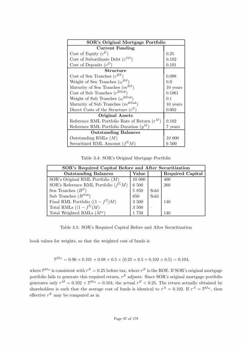
SOR’s Original Mortgage Portfolio

Current FundingCost of Equity (cE) 0.25Cost of Subordinate Debt (cSD) 0.102Cost of Deposits (cD) 0.101

StructureCost of Sen Tranches (cBS) 0.098Weight of Sen Tranches (ωBS) 0.9Maturity of Sen Tranches (mBS) 10 yearsCost of Sub Tranches (cBSub) 0.1061Weight of Sub Tranches (ωBSub) 0.1Maturity of Sub Tranches (mBSub) 10 yearsDirect Costs of the Structure (cΣ) 0.002

Original AssetsReference RML Portfolio Rate of Return (rM ) 0.102Reference RML Portfolio Duration (yM ) 7 years

Outstanding BalancesOutstanding RMLs (M) 10 000Securitized RML Amount (fΣM) 6 500

Table 3.4: SOR’s Original Mortgage Portfolio

SOR’s Required Capital Before and After Securitization

Outstanding Balances Value Required Capital

SOR’s Original RML Portfolio (M) 10 000 400SOR’s Reference RML Portfolio (fΣM) 6 500 260Sen Tranches (BS) 5 850 SoldSub Tranches (BSub) 650 SoldFinal RML Portfolio ((1 − fΣ)M) 3 500 140Total RMLs ((1− fΣ)M) 3 500 –Total Weighted RMLs (Mω) 1 750 140

Table 3.5: SOR’s Required Capital Before and After Securitization

book values for weights, so that the weighted cost of funds is

cMω = 0.96 × 0.101 + 0.08 × 0.5× (0.25 × 0.5 + 0.102 × 0.5) = 0.104,

where cMω is consistent with rE = 0.25 before tax, where rE is the ROE. If SOR’s original mortgage

portfolio fails to generate this required return, rE adjusts. Since SOR’s original mortgage portfolio

generates only rM = 0.102 < cMω = 0.104, the actual rE < 0.25. The return actually obtained by

shareholders is such that the average cost of funds is identical to rA = 0.102. If rA = cMω, then

effective rE may be computed as in

Page 97 of 179

rA = 0.96 × 0.101 + 0.08 × 0.5× (rE × 0.5 + 0.102 × 0.5).

After calculation, rE = 0.15 < 0.25 before tax. In this case, it would be impossible to raise new

capital since the portfolio return does not compensate its risk. Therefore, SOR cannot originate

any additional mortgages without securitization. In addition, the securitization needs to improve

the return to shareholders from (1− fΣ)M.

The potential benefit of securitization is a reduction in cMω. The cost of funds via securitization,

cMΣω, is the weighted cost of the sen and sub tranches (denoted by cBSω and cBSubω, respectively)

plus any additional cost of the structure cΣ = 0.002. Without considering differences in duration,

the cost of sen notes is cBSω = 9.8 % and that of sub notes is cBSubω = 10.61 %. The weighted

average is cMΣω before monitoring and transaction costs, so that

cMΣω = 0.09881 = 0.9× 0.098 + 0.1× 0.1061.

The overall cost of securitization, cMΣωA, is the sum of cMΣω and the annual cΣ = 0.002 averaged

over the life of the deal. The overall costs, cMΣωA, becomes the aggregate weighted cost of funds

via securitization so that

cMΣωA = 0.10081 = cMΣω + 0.002 = 0.09881 + 0.002.

From the above, we draw the following preliminary conclusions. Firstly, we note that cMΣωA =

0.10081 < cMω = 0.104. This is sufficient to make mortgage securitization beneficial. Also, cMΣωA =

0.10081 < rM = 0.102. Therefore, selling SOR’s reference mortgage portfolio to SPV generates a

capital gain which improves SOR’s profitability. However, the change in rE remains to be quantified.

3.5.2.2 Return on Equity (ROE)

The value of SOR’s reference mortgage portfolio, fΣM, is the discounted value of cash flows calcu-

lated at a rate equal to the required return to SORs, rB. The average required return to SORs who

buy SPV’s securities is rB = 0.10081 = cMΣωA. For SOR’s lenders and shareholders, the average

return on SOR’s unsecuritized mortgage portfolio is rls = 0.102. Nevertheless, existing shareholders

would like to have rE = 0.25 instead of rE = 0.15 resulting from insufficient rA = 0.102. In order to

obtain rE = 0.25, SOR’s ROA should be higher and reach rA = 0.104. The present value of fΣM

for SORs is the discounted value of future flows at δ = 0.1008. The value of this mortgage portfolio

for those who fund it results from discounting the same cash flows at δ = 0.102, either with the

current effective rE = 0.15 or δ = 0.104, with a required rE = 0.25. In both cases, cMΣω > cMω.

Therefore, the price of SOR’s reference mortgage portfolio, at the δ = 0.1008 discount rate required

by SORs, will be higher than the price calculated with either δ = 0.102 or δ = 0.104. The difference

is a capital gain for SOR’s existing shareholders. Since the details of projected cash flows generated

by fΣM are unknown, an accurate calculation of its present value is not feasible. In practice, a

Page 98 of 179

securitization model generates the entire cash flows, with all interest received from SOR’s reference

mortgage portfolio, rM , voluntary and involuntary prepayments as well as recoveries.

For this example, we simplify the entire process by circumventing model intricacy for capital struc-

ture. The duration formula offers an easier way to get a valuation for SOR’s reference mortgage

portfolio. We know that the discounted value of future flows generated by SOR’s reference mort-

gage portfolio at rA = 0.102 is exactly 1000 because its return is 0.102. With another discount rate,

the present value differs from this face value. An approximation of this new value can be obtained

from the duration formula via

p1fΣM − 100

100=

−Duration

(1 + i)(δ − rM ),

where the present value of SOR’s reference mortgage portfolio is denoted by p1fΣM. In this case,

the rate of return from fΣM is rM and the discount rate is δ, while the ratio (p1fΣM − 100)/100

provides this value as a percentage of the face value, M. The duration formula provides p1fΣM

given all three other parameters so that

p1fΣM(% of Face Value) = 100 %+ Duration(rM %− δ %).

Since rM = 0.102, the value of fΣM at the discount rate δ = 10.08 % is

p1fΣM = 1 + 7× (0.102 − 0.1008) = 1.0084.

This means that the sale of mortgages to the securitization structure generates Kes = 0.0084 over

an amount of 6 500 or 54.6 in value.

The sale SOR’s reference mortgage portfolio will generate a capital gain only when cMΣωA < µM =

0.102, so that

cMΣωA < cMω.

In this case, the capital gain from the sale of fΣM will effectively increase revenues, thereby

increasing the average rA on the balance sheet. This is a sufficient condition to improve rE under

present assumptions. The reason is that the effective ROE remains a linear function of the effective

rM inclusive of capital gains from the sale of fΣM to SPV, as long as the weights used to calculate

it from rA as a percentage of SOR’s original mortgage portfolio remain approximately constant.

This relation remains

rA = 0.96 × 0.101 + 0.08 × 0.5× (rE × 0.5 + 0.102 × 0.5).

Page 99 of 179

This is true as long as E ∝ fΣM, which is the case in this example. However, in general, Ke 6∝ fΣM,

and the linear relationship collapses. One has to take uncertainty into account if one is required

to determine the effective rE. Note that current cMω = 0.102, by definition, since it equates rM

with the weighted average cost of capital: effective percentage of rA of effective percentage of cMω.

The implied return to shareholders is rls = 0.15. Whenever, cMΣωA < rM , it is by definition lower

than the effective cMω. If the shareholders obtain rE = 0.25, instead of the effective rE = 0.15

only, cMω = 0.104. This securitization would be profitable as long as cMΣωA < 0.104. Since, in this

case, cMΣωA = 0.1008, the deal meets both conditions. However, the first one only is sufficient to

generate capital gain. Using the current effective rE = 0.15, we find that SOR’s capital gain from

selling mortgages is 0.0084 as shown in Table 3.6 below.

SOR’s Cost Benefits from Mortgage Securitization

cMω 0.102cBSub 0.1061cMΣω 0.0988cMΣωA 0.1008SOR’s Reference RML Portfolio Value at cMω 1SOR’s Reference RML Portfolio Value at cMΣωA 1.0084Kes 0.0084

Table 3.6: SOR’s Costs and Benefits from Mortgage Securitization

It is possible to convert Kes from securitization into an additional annualized margin obtained

over the life of the deal. A simple proxy for this annual margin is equal to the instantaneous

capital gain averaged over the life of the deal (ignoring the time value of money). The gain is

Kes = 54.6 = 0.0084 × 6500. This implies that subsequent to securitization, SOR’s reference

mortgage portfolio provide rM = 0.102 plus an annual return of Kes = 0.0084 applicable only to

fΣM = 6500. Once SOR’s original mortgage portfolio have been securitized, the size of the balance

sheet drops to 3 500 that still provides rM = 0.102. There is an additional return due to the capital

gain. Since this annualized capital gain is Kes = 0.0084 of 6 500, it is (0.0084/6500) × 3500 in

percentage of (1− fΣ)M or 0.000001292 applicable to 3 500. Accordingly rM = 0.102 increases to

rM = 0.102001292 after mortgage securitization. This increased rM also implies a higher rE (see

Subsection 3.5.2.3 below).

3.5.2.3 Enhancing ROE Via Securitization

Under a forfeit valuation of capital as a function of fΣM, it is relatively easy to determine whether

the securitization enhances rE, by how much and what the limitations are. Under full economic

analysis, the capital results from a direct calculation of SOR’s reference and unsecuritized mortgage

portfolios. The enhancement issue consists of finding out whether the securitization enhances

the risk-return profile of SOR’s original mortgage portfolio and, more practically, whether post-

securitization rE is higher or lower than pre-securitization rE. We address both these issues in the

sequel.

Table 3.7 shows the income statement under SOR’s reference and unsecuritized mortgage portfo-

lios. The deposits, subordinate debt and equity represent the same percentages of SOR’s original

Page 100 of 179

mortgage portfolio, viz., 96 %, 2 % and 2 %, respectively. Their costs are identical to the above.

Effect of Securitization on SOR’s Return on Capital

Balances Returns and Costs (%) Returns and Costs

Pre-Securitization of 6 500

RMLs 10 000 0.102 1020Deposits 9 600 -0.101 -969.6Equity Capital 200 30Subordinate Debt 200 -0.101 -20.2Return on Capital 0.15

RMLs 3 500 0.102001292 357.0Deposits 3 360 -0.101 -339.36Equity Capital 70Subordinate Debt 70 -0.101 -7.07Return on Capital 0.20263

RMLs 3 500 0.102001292 357.0Deposits 3 360 -0.101 -339.36Equity Capital 190 29.9991Subordinate Debt 190 -0.101 -19.19Return on Capital 0.15789

Table 3.7: Effect of Securitization on SOR’s Return on Capital

Before SOR’s original mortgage portfolio is securitized, rM = 0.102 while thereafter rM = 0.102001292.

This gain influences the ROE directly with an increase from rE = 0.15 to rE = 0.20263. In gen-

eral, an increase in rM causing an increase in rE is not guaranteed since Kes is the marginal risk

contribution of fΣM. Therefore, an increase in rM due to Kes from the sale of SOR’s reference

mortgage portfolio to SPV might not increase the rE if Kes is lower. For instance, if K decreases

to 190 and subordinate debt does also, the remaining deposits being the complement to 9 000 or

9 620, the same calculations would show that the new ROE becomes rE = 0.15789 = 30/190. It

is necessary to determine Ke before and after SOR’s original mortgage portfolio is securitized in

order to determine the size of Kes and to perform return calculations on new capital subsequent to

securitization. Once Ke is determined and converted into a percentage of SOR’s original mortgage

portfolio, we have the same type of formula as in the above.

3.5.3 Example of a Subprime RMBS Bond Deal

The example contained in this subsection explains a subprime RMBS bond deal related to the

Structured Asset Investment Loan Trust 2005-6 (SAIL 2005-6) issued in July 2005 (compare with

[53]). The example considers the evolution of different tranches’ riskiness with the refinancing of

reference mortgage portfolios affecting the loss triggers for subordinated tranches. This changes

the sensitivity of the values of different claims to house prices that drive collateral values. Later

the example goes on to discuss the Structured Asset Investment Loan Trust 2006-2 (SAIL 2006-2).

The bond capital structure is outlined in Table 3.8 below.

Page 101 of 179

Structured Asset Investment Loan Trust 2005-6 Capital Structure

Class RML Principal Principal Tranche Moody’s S&P FitchReference Type Amount ThicknessPortfolios (Dollars) (%)

A1 1 Senior 455 596 000 20.18 % Aaa AAA AAAA2 1 Senior 50 622 000 2.24 % Aaa AAA AAAA3 2 Senior 506 116 000 22.42 % Aaa AAA AAAA4 3 Senior 96 977 000 4.30 % Aaa AAA AAA

Seqntl PayA5 3 Senior 45 050 000 2.00 % Aaa AAA AAA


3 Seqntl PayA7 4 Senior 432 141 000 19.14 % Aaa AAA AAA



Seqntl Pay

M1 1,2,3,4 Subordinated 68 073 000 3.02 % Aa1 AA+ AA+M2 1,2,3,4 Subordinated 63 534 000 2.81 % Aa2 AA AAM3 1,2,3,4 Subordinated 38 574 000 1.71 % Aa3 AA- AA-M4 1,2,3,4 Subordinated 34 036 000 1.51 % A1 A+ A+M5 1,2,3,4 Subordinated 34 036 000 1.51 % A2 A AM6 1,2,3,4 Subordinated 26 094 000 1.16 % A3 A- A-M7 1,2,3,4 Subordinated 34 036 000 1.51 % Baa2 BBB BBBM8 1,2,3,4 Subordinated 22 691 000 1.01 % Baa3 BBB- BBB-M9 1,2,3,4 Subordinated 11 346 000 0.50 % N/R BBB- BBB-

M10-A 1,2,3,4 Subordinated 5 673 000 0.25 % N/R BBB- BB+M10-F 1,2,3,4 Subordinated 5 673 000 0.25 % N/R BBB- BB+

Table 3.8: Structured Asset Investment Loan Trust 2005-6 Capital Structure; Source: [116]

From Table 3.8 we see that the majority of tranches in SAIL 2005-6 have an investment-grade

rating of BBB- or higher with Class A1 to A9 certificates being rated AAA. On a pro rata basis,

Class A1 and A2 certificates receive principal payments, 1fΣM, concurrently, unless cumulative

reference mortgage portfolio losses or delinquencies exceed specified levels. In the latter case, these

classes will be treated as senior, sequential pay tranches.

The classes of certificates listed in Table 3.8 were offered publicly by the SAIL 2005-6 prospectus

supplement while others like Class P, Class X and Class R certificates were not. Four types of

reference mortgage portfolios constitute the deal with limited cross-collateralization. Principal

payments, 1fΣM, on the senior certificates will mainly depend on how the reference mortgage

portfolios are constituted. However, the senior certificates will have the benefit of CE in the form

of overcollateralization (OC) and subordination from each mortgage portfolio. As a consequence,

if the rate of loss per reference mortgage portfolio related to any class of sen certificates is low,

losses in unrelated mortgages may reduce the loss protection for those certificates.

Page 102 of 179

At initiation, we note that the mezz tranches (AA+ to BBB-) were very thin with minimal defaults.

This thinness may be offset by a significant prepayment amount, 2fpfΣM, entering the deal

at the outset. An example of this is the M9 tranche with a thickness of 50 bps, but with a

BBB- investment-grade rating. Although the rating may not necessarily be wrong, the underlying

assumption is that the cash flow dynamics of SAIL 2005-6 has a high probability of success.

Some of the characteristics of the reference mortgage portfolios are shown below.

Summary of the Reference RML Portfolios’ Characteristics

Pool 1 Pool 2 Pool 3 Pool 4

% First Lein 94.12 % 98.88 % 100.00 % 93.96 %% 2/28 ARMs 59.79 % 46.68 % 75.42 % 37.66 %% 3/27 ARMs 20.82 % 19.14 % 19.36 % 9.96 %% Fixed Rate 13.00 % 8.17 % 2.16 % 11.46 %% Full Doc 59.98 % 56.74 % 44.05 % 35.46 %% Stated Doc 39.99 % 37.47 % 34.30 % 33.17 %% Primary Residence 90.12 % 90.12 % 80.61 % 82.59 %WA FICO 636 615 673 635

Table 3.9: Summary of the Reference Mortgage Portfolios’ Characteristics; Source: [53]

3.5.4 Comparisons Between Two Subprime RMBS Deals

In this subsection, we follow [53] by considering the subprime securitization deals Ameriquest Mort-

gage Securities Inc. 2005-R2 (AMSI 2005-R2) and Structured Assets Investment Loan Trust 2006-2

(SAIL 2006-2). Both AMSI 2005-R2 and SAIL 2006-2 possess the basic structures of securitiza-

tion deals outlined in Subsection 3.5.3, with OC and various triggers determining the features of

CE. In this regard, we provide an argument about how the speed of securitization effects the op-

tionality of RMBS CDO tranches with respect to the underlying house prices in both deals. We

note that AMSI 2005-R2 consists of three reference portfolios while both deals have OC. Our aim

is to compare the performance of AMSI 2005-R2 and SAIL 2006-2 with 2005 vintage mortgages

and 2006 vintage mortgages, respectively. For instance, we demonstrate that the latter vintage

subprime mortgages under-performed as house prices began to decline in that year. The ensuing

examples also demonstrate how the extent of refinancing of the reference mortgage portfolios affects

securitization.

3.5.4.1 Details of AMSI 2005-R2 and SAIL 2006-2

Tables 3.10 and 3.11 present AMSI 2005-R2 deal structure, tranche thickness and ratings at the

outset as well as in Q1:07. The initial thickness of the BBB tranches – measured as a percentage

of collateral – are extremely thin. CRAs do not usually allow such thin tranches, but it was

anticipated that these tranches will grow as more sen tranches amortize as a result of refinancing

and sequential amortization. Further, we note the subordination percentages for BBB tranches

at inception. For instance, the M9 tranche of AMSI 2005-R2 was only 2.95 % of subordination.

However, as amortization occurs, CE accumulates and reference mortgages refinance, this situation

Page 103 of 179

could improve. In that case, the deals shrink as amortization occurs. Also, after the step-down

date, the BBB tranches will seem attractive – depending on H.

Ameriquest Mortgage Securities Inc. 2005-R2 (AMSI 2005-R2) At Issue in 2005

Size Related Ratings % of SubordinationMortgage (Fitch, Moody’s CollateralPool(s) S&P)

Publicly-Offered Certificates

A-1A 258 089 000 I AAA/Aaa/AAA 21.5 % 35.48 %A-1B 64 523 000 I AAA/Aaa/NR 5.4 % 19.35 %A-2A 258 048 000 II AAA/Aaa/AAA 21.5 % 35.48 %A-2B 64 511 000 II AAA/Aaa/NR 5.4 % 19.35 %A-3A 124 645 000 III AAA/Aaa/AAA 10.4 % 19.35 %A-3B 139 369 000 III AAA/Aaa/AAA 11.6 % 19.35 %A-3C 26 352 000 III AAA/Aaa/AAA 2.2 % 19.35 %A-3D 32 263 000 III AAA/Aaa/NR 2.7 % 19.35 %M1 31 200 000 I,II,III AA+/Aa1/AA+ 2.6 % 16.75 %M2 49 800 000 I,II,III AA/Aa2/AA 4.1 % 12.6 %M3 16 800 000 I,II,III AA-/Aa3/AA- 1.4 % 11.2 %M4 28 800 000 I,II,III A+/A1/A+ 2.4 % 8.8 %M5 16 800 000 I,II,III A/A2/A 1.4 % 7.4 %M6 12 000 000 I,II,III A-/A3/A- 1.0 % 6.4 %M7 19 200 000 I,II,III BBB+/Baa1/BBB+ 1.6 % 4.8 %M8 9 000 000 I,II,III BBB/Baa2/BBB 0.7 % 4.05 %M9 13 200 000 I,II,III BBB/Baa2/BBB- 1.1 % 2.95 %

Non-Publicly-Offered Certificates

M10 7 800 000 I,II,III BB+/Ba1/BB+ 1.0 % 1.3 %M11 12 000 000 I,II,III BB/Ba2/BB 1.3 % 0.0 %CE 15 600 000 NR/NR/NRTotal 1 200 000 000

Collateral 1 200 000 147

Table 3.10: Ameriquest Mortgage Securities Inc. 2005-R2 (AMSI 2005-R2) At Issue in 2005; Source:[6]

Page 104 of 179

Ameriquest Mortgage Securities Inc. 2005-R2 (AMSI 2005-R2) In Q1:07



A-1A 30 091 837 I AAA/Aaa/AAA 8.3 % 91.67 %A-1B 7 523 047 I AAA/Aaa/NA 2.1 % 89.58 %A-2A 43 208 414 II AAA/Aaa/AAA 12.0 % 77.62 %A-2B 10 801 936 II AAA/Aaa/NA 3.0 % 63.56 %A-3A – III PIF/WR/NR 0.0 % 63.56 %A-3B 9 597 506 III AAA/Aaa/AAA 2.7 % 63.56 %A-3C 26 352 000 III AAA/Aaa/AAA 7.3 % 63.56 %A-3D 3 994 403 III AAA/Aaa/AAA 1.1 % 63.56 %M1 31 200 000 I,II,III AA+/Aa1/AA+ 8.6 % 54.92 %M2 49 800 000 I,II,III AA/Aa2/AA 13.8 % 41.13 %M3 16 800 000 I,II,III AA-/Aa3/AA- 4.7 % 36.48 %M4 28 800 000 I,II,III A+/A1/A+ 8.0 % 28.50 %M5 16 800 000 I,II,III A/A2/A 4.7 % 23.85 %M6 12 000 000 I,II,III BBB/A3/A- 3.3 % 20.53 %M7 19 200 000 I,II,III B/Baa1/BBB+ 5.3 % 15.21 %M8 9 000 000 I,II,III B/Baa2/BBB 2.5 % 12.72 %M9 13 200 000 I,II,III B/Baa3/BBB- 3.7 % 9.06 %


M10 7 800 000 I,II,III CCC/Ba1/BB+ 2.2 % 6.90 %M11 12 000 000 I,II,III CCC/Ba2/BB 3.3 % 3.58 %CE 12 928 188 NR/NR/NR 3.6 % 0.00 %Total 361 097 331

Collateral 361 097 430

Table 3.11: Ameriquest Mortgage Securities Inc. 2005-R2 (AMSI 2005-R2) In Q1:07; Source: [6]

In Tables 3.10 and 3.11, the abbreviations PIF, WR and NR are for tranche paid in full, withdrawn

rating and no rating, respectively.

Tables 3.12 and 3.13 present SAIL 2006-2 deal structure, tranche thickness and ratings at the

outset as well as in Q1:07. Once again, the initial thickness of the BBB tranches – measured

as a percentage of collateral – are extremely thin. As far as the subordination percentages for

BBB tranches at inception are concerned, for instance, the M8 tranche of SAIL 2006-2 has only

0.7 % subordination. As before, as amortization occurs, CE accumulates and reference mortgages

refinance, this situation could improve.

Page 105 of 179

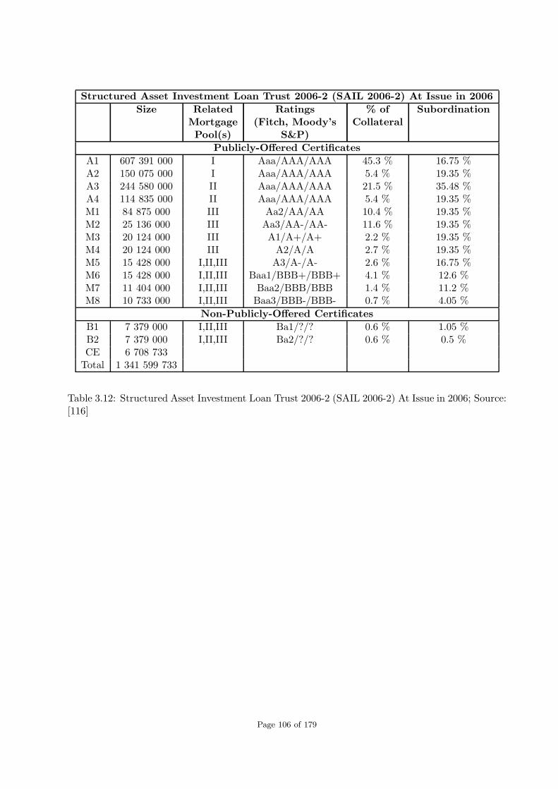
Structured Asset Investment Loan Trust 2006-2 (SAIL 2006-2) At Issue in 2006



A1 607 391 000 I Aaa/AAA/AAA 45.3 % 16.75 %A2 150 075 000 I Aaa/AAA/AAA 5.4 % 19.35 %A3 244 580 000 II Aaa/AAA/AAA 21.5 % 35.48 %A4 114 835 000 II Aaa/AAA/AAA 5.4 % 19.35 %M1 84 875 000 III Aa2/AA/AA 10.4 % 19.35 %M2 25 136 000 III Aa3/AA-/AA- 11.6 % 19.35 %M3 20 124 000 III A1/A+/A+ 2.2 % 19.35 %M4 20 124 000 III A2/A/A 2.7 % 19.35 %M5 15 428 000 I,II,III A3/A-/A- 2.6 % 16.75 %M6 15 428 000 I,II,III Baa1/BBB+/BBB+ 4.1 % 12.6 %M7 11 404 000 I,II,III Baa2/BBB/BBB 1.4 % 11.2 %M8 10 733 000 I,II,III Baa3/BBB-/BBB- 0.7 % 4.05 %


B1 7 379 000 I,II,III Ba1/?/? 0.6 % 1.05 %B2 7 379 000 I,II,III Ba2/?/? 0.6 % 0.5 %CE 6 708 733Total 1 341 599 733

Table 3.12: Structured Asset Investment Loan Trust 2006-2 (SAIL 2006-2) At Issue in 2006; Source:[116]

Page 106 of 179

Structured Asset Investment Loan Trust 2006-2 (SAIL 2006-2) In Q1:07



A1 89 285 238 I Aaa/AAA/AAA 11.0 % 26.16 %A2 150 075 000 I Aaa/AAA/AAA 18.5 % 26.16 %A3 244 580 000 II Aaa/AAA/AAA 30.2 % 26.16 %A4 114 835 000 II Aaa/A/A 14.2 % 26.16 %M1 84 875 000 III Ba3/CCC/B 10.5 % 15.70 %M2 25 136 000 III B3/CCC/CCC 3.1 % 12.60 %M3 20 124 000 III Caa2/CCC/CCC 2.5 % 10.12 %M4 20 124 000 III Caa3/CC/CC 2.5 % 7.36 %M5 15 428 000 I,II,III Ca/CC/CC 1.9 % 5.73 %M6 15 428 000 I,II,III C/CC/CC 1.9 % 3.83 %M7 11 404 000 I,II,III C/CC/C 1.4 % 2.42 %M8 10 733 000 I,II,III C/D/C 1.3 % 1.10 %


B1 7 379 000 I,II,III C/D/C 0.9 % 0.19 %B2 1 534 646 I,II,III WR/NR/NR 0.2 % 0.09 %CE 98 I,II,II 11.0 % 88.99 %Total 810 940 982

Table 3.13: Structured Asset Investment Loan Trust 2006-2 (SAIL 2006-2) In Q1:07; Source: [116]

In Tables 3.12 and 3.13, in addition, there are Class X, P, LT-R and R certificates. The former are

entitled to any monthly excess cashflow left over after contracted payouts to offered certificates and

Class B1 and B2 certificates and payments to the SPV (includes paying swap counterparties) as well

as on and after the distribution date on April 2016 to deposit any final maturity reserve amount

in the final maturity reserve account. On the other hand, Class P certificates will solely be intitled

to receive all prepayment premiums received in relation to the reference mortgage portfolios. Such

amounts are not available for payouts to holders of other certificate classes or to SRs as additional

servicing compensation. The Class LT-R and R certificates will represent the remaining interest in

the assets of the SPV after the required payouts to all other classes of certificates are made. These

classes will evidence the residual interests in the REMIC8.

3.5.4.2 Comparisons Between AMSI 2005-R2 and SAIL 2006-2

Judging from Q1:07, the two deals differ dramatically. AMSI 2005-R2 is older than SAIL 2006-2

and by Q1:07, AMSI 2005-R2 has passed its triggers. As expected, the tranche thicknesses and

subordination levels have increased. For example, initially M9 from the AMSI 2005-R2 deal had

a 2.95 % subordination (1.1 % collateral) level, but by Q1:07 its subordination (collateral) is 9.06

% (3.7 %). Despite this, at the time Fitch downgraded the BBB tranches to B. By contrast, SAIL

8A REMIC (Real Estate Mortgage Investment Conduit) is an investment vehicle – a legal structure that can holdCMLs and mortgages, in trust, and issue securities representing undivided interests in these mortgages. Besides atrust, a REMIC can be a corporation, association or partnership.

Page 107 of 179

2006-2 is younger than AMSI 2005-R2 and took place during a period where house prices were

flat and it was more difficult to refinance. By Q1:07, neither tranche thickness nor subordination

had increased significantly since inception in 2006 thus weakening the SAIL 2006-2 deal. This is

reflected by the mezz tranche ratings.

3.6 Discussions on SubprimeMortgage Securitization and the SMC

In this section, we discuss the relationships between the SMC and risk, profit and valuation under

RMBSs and RMBS CDOs. Also, we comment on examples involving subprime mortgage securi-

tization and its relationships with valuation. In particular, we focus our discussion on the main

hypothesis of this thesis that the SMC was partly caused by the intricacy and design of subprime

mortgage securitization and systemic components that led to information (loss, asymmetry and

contagion) problems, valuation opaqueness and ineffective risk mitigation (compare with Problem

1.3.6 in Section 1.3).

3.6.1 Risk, Profit and Valuation Under RMBSs and the SMC

In this subsection, we discuss the relationships between the SMC and risk, profit and valuation

under RMBSs.

3.6.1.1 Subprime RMBSs and the SMC

The key design feature of subprime mortgages was the ability of MRs to finance and refinance

their houses based on capital gains due to house price appreciation over short horizons and then

turning this into collateral for a new mortgage or extracting equity for consumption. As is alluded

to in Subsection 3.2.1, the unique design of subprime mortgages resulted in unique structures for

their securitizations (response to Problem 1.3.6). During the SMC, CRAs were reprimanded for

giving investment-grade ratings to RMBSs backed by risky subprime mortgages. Before the SMC,

these high ratings enabled such RMBSs to be sold to SIBs, thereby financing and exacerbating the

housing boom. The issuing of these ratings were believed justified because of risk reducing practices,

such as monoline insurance and equity investors willing to bear the first losses. However, during

the SMC, it became clear that some role players in rating subprime-related securities knew at the

time that the rating process was faulty. Uncertainty in financial markets spread to other subprime

agents, increasing the counterparty risk which caused interest rates to increase. Refinancing became

almost impossible and default rates exploded. All these operations embed systemic risk which finally

caused the banking system to collapse (compare with Subsection 3.2.1).

Clearly, during the SMC, the securitization of credit risks was a source of moral hazard that

compromised global banking sector stability. Before the SMC, the practice of splitting the claims

to a reference mortgage portfolio into tranches was a response to this concern. In this case, sen

and mezz tranches can be considered to be senior and junior debt, respectively. If SORs held

equity tranches and if, because of packaging and diversification, the probability of default, i.e.,

the probability that reference portfolio returns do not attain the sum of sen and mezz claims, were

(close to) zero, we would (almost) be neglecting moral hazard effects. How the banking system failed

Page 108 of 179

despite the preceding scenario is explained next (compare with Subsection 3.2.1). Unfortunately, in

reality, both ifs in the statement above were not satisfied. SORs did not, in general, hold the equity

tranches of the portfolios that they generated. In truth, as time went on, ever greater portions

of equity tranches were sold to external SIBs. Moreover, default probabilities for sen and mezz

tranches were significant because packaging did not provide for sufficient diversification of returns

on the reference mortgage portfolios in RMBS portfolios (see, for instance, [58]).

3.6.1.2 Risk and Profit Under RMBSs and the SMC

In the early ’80s, house financing in the U.S. and many European countries changed from fixed-

rate (FRMs) to adjustable-rate mortgages (ARMs) resulting in an interest rate risk shift to MRs.

However, when market interest rates rose again in the late ’80s, SORs found that many MRs

were unable or unwilling to fulfil their obligations at the newly adjusted rates. Essentially, this

meant that the interest rate (market) risk that SORs thought they had eradicated had merely been

transformed into counterparty credit risk. Presently, it seems that the lesson of the ’80s that ARMs

cause credit risk to be higher, seems to have been forgotten or neglected since the credit risk would

affect the RMBS bondholders rather than the SORs (see, for instance, [58]). Subsection 3.2.2.1 of

Subsection 3.2.2 implies that the system of house financing based on RMBSs has some eminently

reasonable features. Firstly, this system permits SORs to divest themselves from the interest rate

risk that is associated with such financing. The experience of the U.S. Savings & Loans debacle

has shown that banks cannot cope with this risk. The experience with ARMs has also shown that

debtors are not able to bear this risk and that the attempt to burden them with it may merely

transform the interest rate risk into counterparty credit risk. Securitization shifts this risk to a

third party.

A subprime mortgage model for profit under subprime RMBSs from (3.2) and (3.4) reflects the

fact that SOR sells mortgages and distributes risk to SIBs through RMBSs. This way of mitigating

risks involves at least operational (including valuation and compensation), liquidity (market) and

tranching (including maturity mismatch) risk that returned to SORs when the SMC unfolded.

SORs are more likely to securitize more mortgages if they hold less capital, are less profitable

and/or liquid and have mortgages of low quality. This situation was prevalent before the SMC

when SORs’ pursuit of yield did not take decreased capital, liquidity and mortgage quality into

account. The investors in RMBSs also embed credit risk which involves bankruptcy if SIBs can’t

raise funds.

In Subsection 3.2.2.2, ΠΣ is given by (3.4) while KΣ has the form (3.5). It is interesting to note

that the formulas for ΠΣ and KΣ depend on Π and K, respectively, and are far more intricate

than the latter. Defaults on RMBSs increased significantly as the crisis expanded from the housing

market to other parts of the economy, causing ΠΣ (as well as retained earnings in (3.3)) to decrease.

During the SMC, capital adequacy ratios declined as KΣ levels became depleted while banks were

highly leveraged. As a consequence, methods and processes which embed operational risk failed. In

this period, such risk rose as banks succeeded in decreasing their capital requirements. Operational

risk was not fully understood and acknowledged which resulted in loss of liquidity and failed risk

mitigation management (compare with Problem 1.3.6).

Page 109 of 179

3.6.1.3 Valuation Under RMBSs and the SMC

When U.S. house prices declined in 2006 and 2007, refinancing became more difficult and ARMs

began to reset at higher rates. This resulted in a dramatic increase in subprime mortgage delinquen-

cies so that RMBSs began to lose value. Since these mortgage products are on the balance sheet of

most banks, their valuation given by (3.8) in Subsection 3.2.3 began to decline (see, also, formulas

(3.6) and (3.7)). Before the SMC, moderate reference mortgage portfolio delinquency did not affect

valuation in a significant way. However, the value of mortgages and related structured products

such as RMBSs decreased significantly due incidences of operational, tranching and liquidity risks

during the SMC. The yield from these structured mortgage products decreased as a consequence

of high default rates (credit risk) which caused liquidity problems with a commensurate rise in the

instances of credit crunch and funding risk (see Subsection 1.2.4 for more details about these risks).

The imposition of fair value accounting for subprime mortgages and their structured products

enhances the scope for systemic risk that involves the malfunctioning of the entire banking system.

Under this type of accounting, the values at which securities are held in banks’ books depend on the

prices that prevail in the market (see formulas (3.6), (3.7) and (3.8) for valuations of banks holding

such securities). In the event of a change in securities prices, the bank must adjust its books even

if the price change is due to market malfunctioning and it has no intention of selling the security,

but intends to hold it to maturity. Under currently prevailing capital adequacy requirements, this

adjustment has immediate implications for the bank’s financial activities. In particular, if market

prices of securities held by the bank have decreased, the bank must either recapitalize by issuing

new equity or retrench its overall operations. The functioning of the banking system thus depends

on how well credit markets are functioning. In short, impairments of the ability of markets to

value mortgages and related structured products such as RMBSs can have a large impact on bank

valuation (compare with Subsection 3.2.3).

3.6.1.4 Optimal Valuation Under RMBSs and the SMC

In Subsection 3.2.4, SIB’s valuation performance criterion, JΣ, at t is given by (3.10). During

the SMC, when valuation was a major issue, JΣ was difficult to compute since the valuation of

components such as B was not easy to determine. In addition, before the SMC, CRAs used

idiosyncratic valuation techniques to give investment-grade ratings to RMBSs despite the fact

the mortgages at face value, mortgage rate, SIB’s optimal deposits and provisions for deposit

withdrawals via Treasuries of the form (3.14), (3.15), (3.16) and (3.17), respectively, computed in

Theorem 3.2.4 – subject to RMBS, balance sheet, cash flow and financing constraints given by

(3.12), (3.13), (3.2) and (3.5), respectively – were clearly suboptimal.

When the capital constraint given by (3.9) holds (i.e., lbt > 0), a solution to the optimal valuation

problem under RMBSs yields optimal profit under RMBSs of the form (3.18). With hindsight, it is

clear that the aforementioned subprime parameters did not compare favorably with their optimal

counterparts. Also, during the SMC, the financing constraint was violated with not enough capital

being held. When the capital constraint (3.9) does not hold (i.e., lbt = 0) and P (Ct) > 0, then

optimal RMBS supply and its rate, (3.26) and (3.27) respectively, are solutions to the optimal

valuation problem stated in Corollary 3.2.5.

Page 110 of 179

3.6.2 Risk, Profit and Valuation Under RMBS CDOs and the SMC

In this subsection, we discuss the relationships between the SMC and capital, information, risk and

valuation under RMBS CDOs. In this regard, Table 3.14 below shows CDO issuance with Column

1 showing total issuance of CDOs while the next column presents total issuance of ABS CDOs.

This table suggests that CDO issuance has been significant both before and after the SMC with

the majority being CDOs with structured notes as collateral. In addition, Table 3.14 suggests that

the motivation for CDO issuance has primarily been arbitrage.

From Table 3.14, we note that issuance of ABS CDOs roughly tripled over the period 2005-07 and

ABS CDO portfolios became increasingly concentrated in subprime RMBSs. In this regard, by 2005,

spreads on subprime BBB tranches seemed to be wider than other structure mortgage products

with the same rating, creating an incentive to arbitrage the ratings between subprime RMBS and

CDO tranches ratings. Subprime RMBSs increasingly dominated CDO portfolios, suggesting that

the pricing of risk was inconsistent with the ratings. Also, concerning the higher rated tranches,

CDOs may have been motivated to buy large amounts of structured mortgage products, because

their AAA tranches would input profitable negative basis trades9. As a consequence, the willingness

of CDOs to purchase subprime RMBS bonds increased. In the period 2008-2009, during the height

of the SMC, there was a dramatic decrease in CDO issuance. During Q1:10 there was a marked

increase in ABS CDO issuance by comparison with Q3:09 and Q4:09 indicating an improvement in

the CDO market.

9According to [53], in a negative basis trade, a bank buys the AAA-rated CDO tranche while simultaneouslypurchasing protection on the tranche under a physically settled CDS. From the bank’s viewpoint, this is the simul-taneous purchase and sale of a CDO security, which meant that IL could book the NPV of the excess yield on theCDO tranche over the protection payment on the CDS. If the CDS spread is less than the bond spread, the basis isnegative. An example of this is given below. Suppose the bank borrows at LIBOR + 5 and buys a AAA-rated CDOtranche which pays LIBOR + 30. Simultaneously, SIB buys protection (possibly from a monoline insurer) for 15 bps(basis points). So SIB makes 25 bps over LIBOR nett on the asset, and they have 15 bps in costs for protection, for a10 bps profit. Note that a negative basis trade swaps the risk of the AAA tranche to a CDS protection writer. Now,the subprime-related risk has been separated from the cash host. Consequently, even if we were able to locate theAAA CDO tranches, this would not be the same as finding out the location of the risk. We do not know the extentof negative basis trades.

Page 111 of 179

Global CDO Issuance ($ Millions)Total Structured Cash Flow Synthetic Arbitrage Balance

Issuance Finance & Hybrid Funded SheetQ1:04 24 982.5 NA 18 807.8 6 174.7 23 157.5 1 825.0Q2:04 42 864.6 NA 25 786.7 17 074.9 39 715.5 3 146.1Q3:04 42 864.6 NA 36 106.9 5 329.7 38 207.7 3 878.8Q4:04 47 487.8 NA 38 829.9 8 657.9 45 917.8 1 569.92004 Tot. 157 418.5 NA 119 531.3 37 237.2 146 998.5 10 419.8% of Tot. 75.9 % 23.7 % 93.4 % 6.6 %Q1:05 49 610.2 28 171.1 40 843.9 8 766.3 43 758.8 5 851.4Q2:05 71 450.5 46 720.3 49 524.6 21 695.9 62 050.5 9 400.0Q3:05 52 007.2 34 517.5 44 253.1 7 754.1 49 636.7 2 370.5Q4:05 98 735.4 67 224.2 71 604.3 26 741.1 71 957.6 26 777.82005 Tot. 271 803.3 176 639.1 206 225.9 64 957.4 227 403.6 44 399.7% of Tot. 65.0 % 75.9 % 23.9 % 83.7 % 16.3 %Q1:06 108 012.7 66 220.2 83 790.1 24 222.6 101 153.6 6 859.1Q2:06 124 977.9 65 019.6 97 260.3 24 808.4 102 564.6 22 413.3Q3:06 138 628.7 89 190.2 102 167.4 14 703.8 125 945.2 12 683.5Q4:06 180 090.3 93 663.2 131 525.1 25 307.9 142 534.3 37 556.02006 Tot. 551 709.6 314 093.2 414 742.9 89 042.7 472 197.7 79 511.9% of Tot. 56.9 % 75.2 % 16.1 % 85.6 % 14.4 %Q1:07 186 467.6 101 074.9 140 319.1 27 426.2 156 792.0 29 675.6Q2:07 175 939.4 98 744.1 135 021.4 8 403.0 153 385.4 22 554.0Q3:07 93 063.6 40 136.8 56 053.3 5 198.9 86 331.4 6 732.2Q4:07 47 508.2 23 500.1 31 257.9 5 202.3 39 593.7 7 914.52007 Tot. 502 978.8 263 455.9 362 651.7 46 230.4 436 102.5 66 8769.3% of Tot. 52.4 % 72.1 % 9.1 % 86.8 % 13.3 %Q1:08 12 846.4 12 771.0 75.4 18 607.1 1 294.6Q2:08 16 924.9 15 809.7 1 115.2 15 431.1 6 561.4Q3:08 11 875.0 11 875.0 – 10 078.4 4 255.0Q4:08 3 290.1 3 140.1 150.0 3 821.4 1 837.82008 Tot. 44 936.4 43 595.8 1 340.6 47 938.0 13 948.8% of Tot. 32.4 % 91.2.1 % 1.6 % 89.4 % 10.6 %Q1:09 296.3 196.8 99.5 658.7 99.5Q2:09 1 345.5 1 345.5 – 1 886.4 –Q3:09 442.9 337.6 105.3 208.7 363.5Q4:09 730.5 681.0 49.5 689.5 429.72009 Tot. 2 815.2 2 560.9 254.3 3 443.3 892.7% of Tot. 40.4 % 91.2.1 % 1.6 % 89.4 % 10.6 %Q1:10 2 420.8 2 378.5 42.3 – 2 420.7Q2:10 1 655.8 1 655.8 – 598.1 1 378.9Q3:10 2 002.7 2 002.7 – 2002.7 –Q4:10 – – – –2010 Tot. 6 079.3 6 037.0 42.3 2 600.8 3 799.6% of Tot. 44.1 % 91.2.1 % 1.6 % 89.4 % 10.6 %

Table 3.14: Global CDO Issuance ($ Millions); Source: [113]

Table 3.15 shows estimates of the typical collateral composition of sen and mezz ABS CDOs before

the SMC. It is clear that subprime and other RMBS tranches make up a sizeable percentage of

both these tranche types.

Page 112 of 179

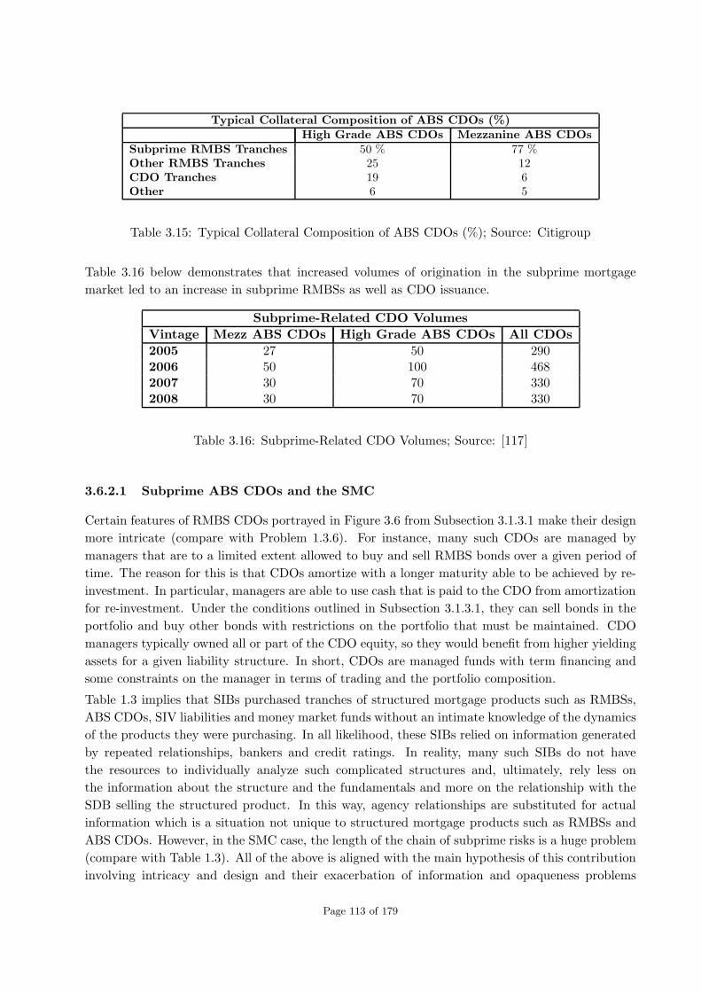
Typical Collateral Composition of ABS CDOs (%)High Grade ABS CDOs Mezzanine ABS CDOs

Subprime RMBS Tranches 50 % 77 %Other RMBS Tranches 25 12CDO Tranches 19 6Other 6 5

Table 3.15: Typical Collateral Composition of ABS CDOs (%); Source: Citigroup

Table 3.16 below demonstrates that increased volumes of origination in the subprime mortgage

market led to an increase in subprime RMBSs as well as CDO issuance.

Subprime-Related CDO Volumes

Vintage Mezz ABS CDOs High Grade ABS CDOs All CDOs

2005 27 50 2902006 50 100 4682007 30 70 3302008 30 70 330

Table 3.16: Subprime-Related CDO Volumes; Source: [117]

3.6.2.1 Subprime ABS CDOs and the SMC

Certain features of RMBS CDOs portrayed in Figure 3.6 from Subsection 3.1.3.1 make their design

more intricate (compare with Problem 1.3.6). For instance, many such CDOs are managed by

managers that are to a limited extent allowed to buy and sell RMBS bonds over a given period of

time. The reason for this is that CDOs amortize with a longer maturity able to be achieved by re-

investment. In particular, managers are able to use cash that is paid to the CDO from amortization

for re-investment. Under the conditions outlined in Subsection 3.1.3.1, they can sell bonds in the

portfolio and buy other bonds with restrictions on the portfolio that must be maintained. CDO

managers typically owned all or part of the CDO equity, so they would benefit from higher yielding

assets for a given liability structure. In short, CDOs are managed funds with term financing and

some constraints on the manager in terms of trading and the portfolio composition.

Table 1.3 implies that SIBs purchased tranches of structured mortgage products such as RMBSs,

ABS CDOs, SIV liabilities and money market funds without an intimate knowledge of the dynamics

of the products they were purchasing. In all likelihood, these SIBs relied on information generated

by repeated relationships, bankers and credit ratings. In reality, many such SIBs do not have

the resources to individually analyze such complicated structures and, ultimately, rely less on

the information about the structure and the fundamentals and more on the relationship with the

SDB selling the structured product. In this way, agency relationships are substituted for actual

information which is a situation not unique to structured mortgage products such as RMBSs and

ABS CDOs. However, in the SMC case, the length of the chain of subprime risks is a huge problem

(compare with Table 1.3). All of the above is aligned with the main hypothesis of this contribution

involving intricacy and design and their exacerbation of information and opaqueness problems

Page 113 of 179

(compare with Problem 1.3.6).

3.6.2.2 Risk and Profit Under RMBS CDOs and the SMC

A subprime mortgage model for profit under subprime RMBS CDOs has the form (3.32) given in

Subsection 3.3.1. Under RMBS CDOs, ΠΣbt is given by (3.33) while capital is of the form (3.34). In

this regard, before the SMC, SIBs sought higher profits than those offered by U.S. Treasury bonds.

Continued strong demand for RMBSs and RMBS CDOs began to drive down lending standards

related to originating mortgages destined for reference portfolios in securitization. RMBS CDOs

lost most of their value which resulted in a large decline in the capital of many banks and GSEs,

with a resultant tightening of credit globally.

As we have seen before, subprime risks and profit play a key role in Subsection 3.3.1. In this regard,

before the SMC, CDOs purchased subprime RMBS bonds because it was profitable. At first,

lower-rated BBB tranches of subprime RMBS were difficult to sell since they were thin and, hence,

unattractive. Later the thickness of these tranches increased and investment in them became more

alluring for SIBs (compare with the examples contained in Subsections 3.5.3 and 3.5.4). Despite this,

a purchasing CDO may not be aware of the subprime risks inherent in the RMBS deal, including

credit and synthetic risk. In this way, risks were underestimated and mortgages and structured

mortgage products were over-rated. In particular, tranching added intricacy to securitization. This

assertion has resonance with the main hypothesis of this contribution involving the intricacy and

design of subprime structured mortgage products and their role in information and opaqueness

problems as well as risk mismanagement (compare with Problem 1.3.6).

3.6.2.3 Valuation Under RMBS CDOs and the SMC

In Subsection 3.3.2, we note that SIB’s value under RMBS CDOs is given by (3.37). In this regard,

to our knowledge, there is no standardization of triggers across CDOs with some having sequential

cash flow triggers while others have OC trigger calculations based on ratings changes. As far as

performing valuations is concerned, in reality, each RMBS CDO must be separately valued which

may not be possible (compare with formula (3.35) for nett cash flow under RMBS CDOs). During

the SMC, this played a role in the problems SIBs faced when they attempted a valuation of CDO

tranches. Furthermore, RMBS CDOs widely held by SDBs and SIBs lost most of their value

during this period. Naturally, this led to a dramatic decrease in SIB’s valuation from holding such

structured mortgage products which, in turn, increased the subprime risks in mortgage markets

(refer to formulas (3.36) and (3.37) for SIB’s valuation under RMBS CDOs).

3.6.2.4 Optimal Valuation Under RMBS CDOs and the SMC

In Subsection 3.3.3, valuation performance criterion, JΣb, in period t is given by (3.38) while the

total capital constraint may be represented by (3.9). The optimal valuation problem under RMBSs

is to maximize value given by (3.37) by choosing the RMBS rate, deposits and regulatory capital for

(3.39) subject to RMBS, balance sheet, cash flow and financing constraints given by (3.12), (3.13),

(3.32) and (3.34), respectively. When the capital constraint given by (3.9) holds (i.e., lbt > 0),

a solution to the optimal valuation problem yields optimal RMBSs and RMBS rates of the form

Page 114 of 179

(3.14) and (3.15), respectively. Most importantly, all the comments in Subsection 3.6.1.4 about

optimal valuation under RMBSs can be repeated for RMBS CDOs.

The optimal valuation formulas mentioned above can be used to illustrate how information is lost

due to intricacy. For RMBS CDO investors, the fact that information is lost implies that it is

impossible for them to penetrate the chain backwards and value the chain based on the reference

mortgage portfolios. RMBS CDO design itself does not allow for valuation based on the reference

mortgage portfolio. This is due to the fact that there are at least two layers of structured products

in CDOs. Information is lost because of the difficulty of penetrating to the core assets. Nor is it

possible for those at the start of the chain to use their information to value the chain ”forwards”

in a manner of speaking (compare with the analysis in Subsection 3.3.3).

3.6.3 Mortgage Securitization and Capital Under Basel Regulation and the

SMC

In this subsection, we discuss the connections between Basel capital regulation and the SMC. The

capital constraint in Section 3.4 for the securitized case is described by the expression in (2.13). In

particular, we keep the risk-weights for mortgages are kept constant, i.e., ωM = 1. In this case, the

capital constraint (2.13) becomes (3.48).

An example of the fact that capital was in short supply at the outset of the SMC in the second

half of 2007 is given below. In this period, Citigroup Inc. had its worst-ever quarterly loss of $

9.83 billion and had to raise more than $ 20 billion in capital from outside investors, including

foreign-government investment funds. This was done in order to augment the depleted capital on

its balance sheet after bad investments in structured mortgage products. According to the Federal

Deposit Insurance Corporation (FDIC), at the time, Citigroup held $ 80 billion in core capital

on its balance sheet to protect against its $ 1.1 trillion in assets. In the second half of 2007,

Citigroup wrote down about $ 20 billion. Amazingly, at the end of 2007, major U.S. banks like J.P.

Morgan Chase & Co., Wachovia Corp., Washington Mutual Inc. and Citigroup lobbied for leaner,

European-style capital cushions. These banks argued that tighter rules would make it tougher

for them to compete globally, since more of their money would be tied up in the capital cushion.

Eventually, in July 2008, the U.S. Federal Reserve and regulators acceded to the banks’ requests

by allowing them to follow rules similar to those in Europe. That ruling enabled U.S. banks to

hold looser, European-style capital. However, by then, cracks in the global banking system were

already spreading rapidly.

3.6.3.1 Quantity and Pricing of Mortgages and Capital Under Basel Regulation (Se-

curitized Case) and the SMC

In Subsection 3.4.1, we considered how capital, K, and the quantity and price of RMBSs, B, are

affected by changes in the level of credit rating, CB , when risk-weight on RMBSs, ω(CBt ), are allowedto vary.

During the SMC, as banks adjusted to mortgage delinquencies and defaults and the breakdown

of maturity transformation, the interplay of market malfunctioning or even breakdown, fair value

accounting and the insufficiency of equity capital, and, finally, systemic effects of prudential regu-

Page 115 of 179

lation created a detrimental downward spiral in the banking system. By contrast, critical securities

are now being traded in markets, and market prices determine the day-to-day assessments of equity

capital positions of institutions holding them.

Systemic risk explains why the SMC has turned into a worldwide financial crisis unlike the S&L

crisis of the late eighties. There were warnings at the peak of the S&L crisis that overall losses

of US savings institutions might well amount to $ 600-800 billion. This is no less than the IMF’s

estimates of losses in subprime RMBSs. However, these estimates never translated into market

prices and the losses of the S&Ls were confined to the savings institutions and to the deposit

insurance institutions that took them over. This difference in institutional arrangements explains

why the fallout from the current crisis has been so much more severe than that of the S&L crisis.

3.6.3.2 Subprime Mortgages and Their Rates Under Basel Capital Regulation (Slack

Constraint; Securitized Case) and the SMC

In Subsection 3.4.2 we consider the effect of a shock to RMBS credit rating CBt , on B, and rB . In

particular, we analyze the case where the capital constraint (3.48) is slack. When lbt = 0 we have

(3.53) and (3.54).

Before the SMC, there was a relative decline in equity related to the capital that banks held in

fulfilment of capital adequacy requirements as well as the buffers that they held in excess of required

capital. A decline in required capital was made possible by changes in statutory rules relating to

the prudential regulation of bank capital. The changes in rules provided banks with the option

to determine regulatory capital requirements by assessing value-at-risk in the context of their own

quantitative risk models, which they had developed for their own risk management. In particular,

internationally active banks were able to determine capital requirements for market risks on the

basis of these internal models. The amount of capital they needed to hold against any given asset

was thereby greatly reduced.

3.6.3.3 Subprime Mortgages and Their Rates Under Basel Capital Regulation (Hold-

ing Constraint; Securitized Case) and the SMC

Subsection 3.4.3 present results about the effect of changes in the level of credit rating, CB , onRMBSs when the capital constraint (3.48) holds. If lbt > 0 then by taking the first derivatives of

equation (3.14) with respect to CBt and using the fact that the risk-weights for mortgages, ωM , are

constant we obtain (3.55). In this situation, the subprime RMBS payout rate response to changes

in the level of credit rating is given by (3.56).

Unlike in the 19th century, there is no modern equivalent to clearing houses that allowed information

asymmetry to dissipate. During the SMC, there was no information producing mechanism that

was implemented. Instead, accountants follow rules by, for instance, enforcing ”marking.” Even for

earlier vintages, accountants initially seized on the ABX indices in order to determine ”price,” but

were later willing to recognize the difficulties of using ABX indices. However, marking-to-market

implemented during the SMC, has very real effects because regulatory capital and capital for CRA

purposes is based on generally accepted accounting principles (GAAP). The GAAP measure of

capital is probably a less accurate measure of owner-contributed capital than the Basel measure of

Page 116 of 179

capital since the latter takes into account banks’ exposure to credit, market and operational risk

and their off-balance sheet activities. There are no sizeable platforms that can operate ignoring

GAAP capital. During the SMC, partly as a result of GAAP capital declines, banks are selling

large amounts of assets or are attempting to sell assets to clean up their balance sheets, and in so

doing raise cash and de-levering. This pushes down prices, and another round of marking down

occurs and so on. This downward spiral of prices – marking down then selling then marking down

again – is a problem where there is no other side of the market (see, for instance, [58]).

3.6.3.4 Subprime Mortgages and Their Rates Under Basel Capital Regulation (Fu-

ture Time Periods; Securitized Case) and the SMC

In Subsection 3.4.4 we examine the effect of a current credit rating shock in future periods on

subprime RMBSs, B, and their payout rates, rB. The response of subprime RMBSs and RMBS

rates to a change in the level of credit rating, CBt , is described by (3.57) if the capital constraint

holds. Most importantly, all the comments about subprime mortgages and their rates under Basel

capital regulation for RMBSs can be repeated for RMBS CDOs.

The incidence of systemic risk in the SMC has been exacerbated by an insufficiency of equity capital

held against future mortgage losses. As the system of risk management on the basis of quantitative

risk models was being implemented, banks were becoming more conscious of the desirability of

”economizing” on equity capital and of the possibility of using the quantitative risk models for this

purpose. Some of the economizing on equity capital involved improvements in the attribution of

equity capital to different activities, based on improvements in the awareness and measurement

of these activities’ risks. Some of the economizing on equity capital led to the relative decline in

equity that is one of the elements shaping the dynamics of the downward spiral of the financial

system since August 2007. One may assume that the loss of resilience that was caused by the

reduction in equity capital was to some extent outweighed by the improvements in the quality of

risk management and control. However, there may also have been something akin to the effect that

the instalment of seat belts or anti-blocking systems in cars induces people to drive more daringly.

A greater feeling of protection from harm or a stronger sense of being able to maintain control may

induce people to take greater risks.

3.6.4 Examples Involving Subprime Mortgage Securitization and the SMC

In this subsection, we discuss the relationships between the SMC and a numerical example involving

mortgage securitization, securitization economics, an example of a subprime RMBS deal as well as

a comparison between two typical subprime deals.

3.6.4.1 Numerical Example Involving Subprime Mortgage Securitization and the

SMC

The example in Subsection 3.5.1 shows that under favorable economic conditions (for instance,

where RMBS default rates are low and CB is high) huge profits can be made from securitizing

subprime RMBSs as was the case before the SMC. On the other hand, during the SMC, when

Page 117 of 179

conditions are less favorable (for instance, where RMBS default rates are high and CB is low), SIBs

suffer large mortgage securitization losses.

We observe from the numerical example that costs of funds and capital constraints from Basel

capital regulation have important roles to play in subprime mortgage securitization, profit and

valuation. We see that the profit under securitization in period t+ 1 is less than the profit under

securitization in period t. This is mainly due to higher reference RMBS portfolio defaults as a result

of higher RMBS rates in period t+ 1. This was a major cause of the SMC.

3.6.4.2 Example Involving Profit from Mortgage Securitization and the SMC

The part of our example of mortgage securitization in Subsection 3.5.2.1, does not suggest that

it is generally true that all outcomes will be favorable, because it is possible that cMΣω < cMω,

but is still higher than the reference mortgage portfolio return, rM , thereby generating a loss when

selling mortgages to SPV. Even if cMΣω > cMω, there would be room to improve SOR’s portfolio rE

because ofKes. As a consequence the discussion presented in Subsection 3.5.2.1 is not representative

of all possible situations.

In Subsection 3.5.2.2, we note that the influence on rE is from both lower level E and reduced

cMΣωA. The gain value is either present value or an improvement of annual margins averaged over

the life of the deal. In the example, Kes is a present forfeit percentage of 4 % used as an input.

When considering the SMC, this same percentage of mortgages could result from modeling Ke and

could be an output of a mortgage portfolio model. In both cases, an analysis of the securitization

economics should strive to determine whether securitization improves the risk-return profile of

SOR’s original mortgage portfolio. Enhancing the risk-return profile means optimizing the efficient

frontier or increasing rE for SOR’s reference mortgage portfolio. We may ascertain whether this is

true by calculating rE and rEΣ as well as comparing them.

From Subsection 3.5.2.3, if securitization improves rE , SOR’s might be inclined to increase fΣM.

Potentially, SOR could benefit even more from the good relationship between fΣM and rE – known

as the leverage effect of securitization. Leverage is positive as long as cMΣω = 0.1008 remains fixed

with a higher fΣM leading to a higher final rE subsequent to securitization. For instance, using the

example in Subsection 3.5.2.3, securitizing 2 000 instead of 1 000, and keeping the same proportions

of mortgages to D and K, would automatically increase rE. This increase does not result from an

additional capital gain in fΣM, since this gain remains 0.00833 of mortgages. Instead it results from

the fact that the additional annualized rate of return, ra, is proportional to the ratio of mortgages

before and after securitization. In the example, with fΣM = 1000, ra as a percentage of fΣM is

ra = 0.000926 = 0.00833 × 1000/9000

of mortgages. Should SOR sell 2 000, the same percentage of fΣM would increase to 0.001851 =

0.00833×2000/9000, the earnings before tax (EBT) would become rE = 0.33346 and the return on

capital (now 160) would be rK = 0.0020841 = 0.33346/160. Another simulation will demonstrate

that fΣM = 5000, would provide an rE = 0.23965 and rK = 0.23965. In fact, fΣM = 5553, would

allow hitting the 25 % target return on (1 − fΣ)M. This is the leverage effect of securitization,

Page 118 of 179

which is more than proportional to fΣM. We note that there are limits to this leverage effect.

Firstly, an SOR securitizing all mortgages (i.e., fΣ = 1 as in true-sales securitization) changes its

core operations by becoming a pure SOR reselling new business to SPVs. As in the OTH model,

origination and lending, collecting deposits and providing financial services to customers are the

core business of commercial banking. Keeping mortgages on the balance sheet is part of the core

business. This is a first reason for SOR not going to the extreme by securitizing its entire balance

sheet. Secondly, SORs need to replenish the portfolio of securitized receivables. In order to do so,

they need to keep assets on the balance sheet. This happens, for instance, when securitizing credit

cards that amortize much quicker than mortgages. In such cases, the pool of credit card receivables

rolls over with time and fluctuates depending on the customers’ behavior. SOR needs a pool of such

receivables to replenish its reference mortgage portfolio. Thirdly, increasing securitization would

result in significant changes in operations and might change SORs’ perception by, for instance,

modifying its cost of funds. This may or may not be true depending on how Kes is utilized.

3.6.4.3 Example of a Subprime RMBS Bond Deal and the SMC

From Table 3.8 in Subsection 3.5.3, for the structure of SAIL 2005-6, we can deduce that there

are four reference mortgage portfolios with limited cross-collateralization. This deal took place

immediately prior to the onset of the SMC in mid-2007. Furthermore, it is obvious that princi-

pal payments on the sen certificates will largely depend on collections on the reference mortgage

portfolios. Thus, even if the loss rate per reference portfolio related to any sen certificates class

is low, losses in unrelated mortgages may reduce the loss protection for those certificates. This is

so because the sen certificates will have the benefit of CE in the form of OC and subordination

from each mortgage pool. This is typically what happened during the SMC with toxic mortgages

reducing protection for sen certificates.

Initially, the mezz tranches are thin and small with respect to defaults. This makes the investment-

grade rating BBB- of these tranches somewhat surprising. This may be offset by a significant

amount of prepayment, 2fpfΣM, coming into the SAIL 2005-6 deal at the onset. Despite the

fact that the underlying supposition is that the deal’s cash flow dynamics has a high probability of

success, the accuracy of these ratings are being questioned in the light of the SMC. The procedure

by which 2fpfΣM from fΣM are allocated will differ depending on the occurrence of several

different triggers10 given in Subsection 3.5.3. As noted in [53] and described in the SAIL 2005-6

prospectus supplement, the triggers have the following specifications.

• whether a distribution date occurs before or on or after the step-down date, which is the latter

of the (1) distribution date in July 2008 and (2) first distribution date on which the ratio

Total Principal Balance of the Subordinate Certificates Plus Any OC Amount

Total Principal Balance of the mortgages in the Trust Fund

equals or exceeds the percentage specified in this prospectus supplement;

• a cumulative loss trigger event occurs when cumulative losses on the mortgages are higher than

certain levels specified in this prospectus supplement;

10Some of these triggers were simply ignored before and during the SMC.

Page 119 of 179

• a delinquency event occurs when the rate of delinquencies of the mortgages over any 3-month

period is higher than certain levels set forth in this prospectus supplement and

• in the case of reference mortgage portfolio 1, a sequential trigger event occurs if (a) before

the distribution date in July 2008, a cumulative loss trigger event occurs or (b) on or after the

distribution date in July 2008, a cumulative loss trigger event or a delinquency event occurs.

3.6.4.4 Comparisons Between Two Subprime RMBS Deals and the SMC

From the example involving the deals AMSI 2005-R2 and SAIL 2006-2 in Subsection 3.5.4, it is

clear that the thin tranches and low subordination levels at inception are acceptable provided that

the reference mortgages refinance in the anticipated way. In this situation, the RMBS bond deals

shrink as amortization occurs. Also, depending on house prices, CE will build up and after the

step down date, SIBs will consider investing in the BBB tranches.

The features of AMSI 2005-R2 and SAIL 2006-2 illustrate the differences between subprime and

standard securitizations with their fixed tranche sizes and use of XS to create CE through reserve

fund build-up. However, this is not the primary form of CE. In the subprime case, Subsection 3.5.4

illustrates how the option on house prices implicitly embedded in subprime reference mortgage

portfolios resulted in the behavior of subprime RMBSs being sensitive to house prices. By contrast

to standard securitization, the tranche thickness and extent of CE – depend on cash flow coming

into the deal from 2fpfΣM on fΣM via refinancing that is also house price dependent.

The deals AMSI 2005-R2 and SAIL 2006-2 illustrate this link to house price very effectively. The

former passed its triggers and achieved the CE and subordination levels hoped for at inception –

largely due to reference mortgage refinancing and prepayments. By contrast, the SAIL 2006-2 deal

deteriorated. In 2006, subprime MRs did not accumulate enough house equity to refinance with

the result that they defaulted on their repayments. Consequently, SAIL 2006-2 was not able to

pass its triggers.

3.7 2007-2010 Timeline of SMC-Related Events Involving Sub-

prime Mortgage Securitization

In this subsection,we give a timeline of SMC-related events involving subprime mortgage securiti-

zation in the period 2007-2010.

Tuesday, 27 February 2007: Freddie Mac announces that it will no longer buy the most risky

subprime RMLs and securities backed by them.

Friday, 1 June 2007: S&P and Moody’s Investor Services downgrade over 100 bonds backed by

second-lien subprime RMLs.

Thursday, 7 June 2007: Bear Stearns informs investors that it is suspending redemptions from

its High-Grade Structured Credit Strategies Enhanced Leverage Fund.

Monday, 11 July 2007: S&P places 612 securities backed by subprime RMLs on a credit watch.

Page 120 of 179

Tuesday, 31 July 2007: Bear Stearns liquidates two hedge funds that invested in various types

of MBSs.

Monday, 15 October 2007: Citigroup, Bank of America, and JPMorgan Chase announce plans

for an $ 80 billion MLEC to purchase highly rated assets from existing SPVs.

Wednesday, 12 December 2007: FOMC authorizes temporary reciprocal currency arrange-

ments (swap lines) with ECB and SNB. Fed states that it will provide up to $ 20 billion and $ 4

billion to the ECB and SNB, respectively, for up to 6 months.

Friday, 21 December 2007: Citigroup, JPMorgan Chase, and Bank of America abandon plans

for the MLEC announcing that the fund ”is not needed at this time.”

Friday, 2 May 2008: FOMC expands the list of eligible collateral for Schedule 2 TSLF auctions

to include AAA/Aaa-rated asset-backed securities, in addition to already eligible residential and

commercial MBSs and agency collateralized mortgage obligations. FOMC also increases existing

swap lines with ECB by $ 20 billion and SNB by $ 6 billion. FRB expands TAF auctions from $

50 billion to $ 75 billion.

Tuesday, 15 July 2008: SEC issues an emergency order temporarily prohibiting naked short sell-

ing in the securities of Fannie Mae, Freddie Mac, and primary dealers at commercial and investment

banks.

Wednesday, 30 July 2008: FOMC increases its swap line with the ECB to $ 55 billion.

Sunday, 14 September 2008: FRB expands the list of eligible collateral for the PDCF to include

any collateral that can be pledged in the tri-party repo system of the two major clearing banks.

Previously PDCF collateral had been limited to investment-grade debt securities.

Tuesday, 16 September 2008: The net asset value of shares in the RPMF falls below $ 1,

primarily due to losses on Lehman Brothers commercial paper and medium-term notes.

Thursday, 18 September 2008: FOMC expands existing swap lines by $ 180 billion and autho-

rizes new swap lines with the Bank of Japan, BOE, and Bank of Canada.

Friday, 19 September 2008: FRB announces the creation of the AMLF to extend non-recourse

loans at the primary credit rate to U.S. depository institutions and bank holding companies to

finance their purchase of high-quality asset-backed commercial paper from money market mutual

funds. The Federal Reserve Board also announces plans to purchase federal agency discount notes

(short-term debt obligations issued by Fannie Mae, Freddie Mac, and Federal Home Loan Banks)

from primary dealers.

Wednesday, 24 September 2008: FOMC establishes new swap lines with the Reserve Bank of

Australia and the Sveriges Riksbank for up to $ 10 billion each and with the Danmarks National

bank and the Norges Bank for up to $ 5 billion each.

Page 121 of 179

Friday, 26 September 2008: FOMC increases existing swap lines with the ECB by $ 10 billion

and the Swiss National Bank by $ 3 billion.

Monday, 29 September 2008: FOMC authorizes a $ 330 billion expansion of swap lines with

Bank of Canada, BOE, Bank of Japan, Danmarks Nationalbank, ECB, Norges Bank, Reserve Bank

of Australia, Sveriges Riksbank, and SNB swap lines outstanding now total $ 620 billion.

Tuesday, 7 October 2008: FRB announces the creation of CPFF, which will provide a liquid-

ity backstop to U.S. issuers of commercial paper through a SPV that will purchase three-month

unsecured and asset-backed CP directly from eligible issuers.

Monday, 13 October 2008: FOMC increases existing swap lines with foreign central banks.

BOE, ECB and SNB announce that they will conduct tenders of U.S. dollar funding at 7-, 28-, and

84-day maturities at fixed interest rates.

Tuesday, 14 October 2008: Fed announces additional details of CPFF. FOMC increases its

swap line with the Bank of Japan.

Tuesday, 28 October 2008: FOMC and Reserve Bank of New Zealand establish a $ 15 billion

swap line.

Thursday, 29 October 2008: FOMC establishes swap lines with the Banco Central do Brasil,

Banco de Mexico, Bank of Korea, and the Monetary Authority of Singapore for up to $ 30 billion

each.

Friday, 21 November 2008: Treasury announces that it will help liquidate the Fed Fund’s U.S.

Government Fund. Treasury agrees to serve as a buyer of last resort for the fund’s securities to

ensure the orderly liquidation of the fund.

Tuesday, 25 November 2008: Treasury and FRB announce the launch of TALF. Under the

program, the Federal Reserve Bank of New York will lend up to $ 200 billion to eligible owners of

certain AAA-rated ABSs backed by newly and recently originated auto loans, credit card loans,

student loans and small business loans that are guaranteed by SBA.

Wednesday, 2 December 2008: FRB announces that it will extend three liquidity facilities –

PDCF, AMLF and TSLF – until Thursday, 30 April 2009.

Friday, 19 December 2008: FRB announces revised terms and conditions of TALF. Among

the revisions are an extension of TALF loans from maturities of one year to three years and an

expansion of eligible ABS collateral.

Tuesday, 30 December 2008: SEC releases a report that recommends against the suspension

of fair value accounting standards and was mandated by EESA.

Page 122 of 179

Saturday, 5 January 2009: FRBNY begins purchasing fixed-rate MBSs guaranteed by Fannie

Mae, Freddie Mac and Ginnie Mae under a program first announced on Tuesday, 25 November

2008.

Tuesday, 3 February 2009: Swap lines between the Fed and other central banks are also extended

to day, 30 October 2009. The expiration date for the TALF remains Thursday, 31 December 2009,

and the TAF does not have an expiration date.

Friday, 6 February 2009: FRB releases additional terms and conditions of TALF. Under TALF,

the FRBNY will lend up to $ 200 billion to eligible owners of certain AAA-rated ABSs backed

by newly and recently originated auto loans, credit card loans, student loans and SBA-guaranteed

small business loans.

Tuesday, 3 March 2009: Fed and Treasury expect to include ABSs backed by other types of

loans in future monthly TALF fundings.

Thursday, 19 March 2009: FRB announces an expansion of the eligible collateral for loans

extended by TALF to include ABSs backed by mortgage servicing advances, loans or leases related

to business equipment, leases of vehicle fleets, and floorplan loans.

Wednesday, 1 April 2009: Fed chairman, Bernanke, and FRBNY president, Dudley, respond to

questions from the COP about TALF, explaining in detail the rationale and operation of it.

Monday, 6 April 2009: Fed announces new reciprocal currency agreements (swap lines) with

the BOE, ECB, the Bank of Japan and SNB that would enable the provision of foreign currency

liquidity by the Fed to U.S. financial institutions.

Thursday, 9 April 2009: FASB issues three final Staff Positions intended to provide additional

application guidance and enhance disclosures regarding fair value measurements and impairments

of securities.

Friday, 1 May 2009: FRB announces that, starting in June 2009, CMBSs and securities backed

by insurance premium finance loans will be eligible collateral under TALF. FRB also authorizes

TALF loans with maturities of five years.

Wednesday, 13 May 2009: Treasury proposes amendments to the CEA and securities laws to

enhance government regulation of OTC derivatives markets. The proposed changes include require-

ments that all standardized OTC derivatives be cleared through regulated central counterparties,

and that all OTC derivatives dealers and all other firms whose activities in those markets create

large exposures to counterparties be subject to prudential supervision and regulation.

Tuesday, 19 May 2009: FRB announces that, starting in July 2009, certain high-quality CMBSs

issued before Thursday, 1 January 2009 – known as legacy CMBSs – will become eligible collateral

under TALF. The objective of the expansion is to restart the market for legacy securities and, by

Page 123 of 179

doing so, stimulate the extension of new credit by helping to ease balance sheet pressures on banks

and other financial institutions. Eligible CMBSs must have a AAA rating from at least two major

rating services.

Wednesday, 24 June 2009: The Fed announces extensions of and modifications to a number

of its liquidity programs. The expiration date AMLF, CPFF, PDCF and TSLF is extended until

Monday, 1 February 2010. The expiration date of TALF remains set at Thursday, 31 December

2009. In addition, the temporary reciprocal currency arrangements (swap lines) between the Fed

and other central banks have been extended to Monday, 1 February 2010.

Wednesday, 8 July 2009: Treasury, Fed and FDIC announce the details of PPIP. Under this

program, Treasury will invest up to $ 30 billion with private sector fund managers and private

investors for the purpose of purchasing legacy securities. PPIP will participate in the market

for CMBSs and non-agency RMBSs. To qualify for purchase, these securities must have been

issued prior to 2009 and have originally been rated AAA (or an equivalent rating by two or more

nationally recognized statistical rating organizations) without ratings enhancement and must be

secured directly by the actual MLs, leases, or other assets known as eligible assets.

Monday, 17 August 2009: FRB and Treasury announce an extension to TALF. Eligible loans

against newly issued ABSs and legacy CMBSs can now be made until Wednesday, 31 March 2010.

Because new CMBS deals can take a significant amount of time to arrange, TALF lending against

newly issued CMBS was approved until Wednesday, 30 June 2010. The previously-announced

deadline for TALF loans was Thursday, 31 December 2009. Fed and Treasury do not anticipate

any further additions to the types of collateral that are eligible for the TALF.

Thursday, 21 January 2010: FRB and thrift regulatory agencies announce the final risk-based

capital rule related to the Financial Accounting Standards Board’s adoption of Statements of Finan-

cial Accounting Standards Nos. 166 and 167. These new accounting standards make substantive

changes to how banking organizations account for many items, including securitized assets, that

had been previously excluded from these organizations’ balance sheets. Banking organizations af-

fected by the new accounting standards generally will be subject to higher risk-based regulatory

capital requirements. The rule better aligns risk-based capital requirements with the actual risks

of certain exposures. It also provides an optional phase-in for four quarters of the impact on risk-

weighted assets and tier 2 capital resulting from a banking organization’s implementation of the

new accounting standards

Tuesday, 16 March 2010: To provide support to mortgage lending and housing markets and to

improve overall conditions in private credit markets, the Federal Reserve has been purchasing $1.25

trillion of agency mortgage-backed securities and about $175 billion of agency debt; those purchases

are nearing completion, and the remaining transactions will be executed by the end of this month.

The Committee will continue to monitor the economic outlook and financial developments and will

employ its policy tools as necessary to promote economic recovery and price stability. In light of

improved functioning of financial markets, the Federal Reserve has been closing the special liquidity

facilities that it created to support markets during the crisis. The only remaining such program,

Page 124 of 179

the Term Asset-Backed Securities Loan Facility, is scheduled to close on June 30 for loans backed

by new-issue commercial mortgage-backed securities and on March 31 for loans backed by all other

types of collateral.

Wednesday, 17 March 2010: The federal banking agencies, in conjunction with the Conference

of State Bank Supervisors (CSBS), released a policy statement on their expectations for sound

funding and liquidity risk management practices. This policy statement, adopted by each of the

agencies, summarizes the principles of sound liquidity risk management issued previously and,

when appropriate, supplements them with the ”Principles for Sound Liquidity Risk Management

and Supervision” issued in September 2008 by the Basel Committee on Banking Supervision.

Friday, 30 April 2010: The federal financial regulatory agencies issued final guidance to address

the risks associated with funding and credit concentrations arising from correspondent relation-

ships. A correspondent relationship occurs when a financial organization provides another financial

organization with services related to deposits, lending, or other activities. The guidance highlights

the need for institutions to identify, monitor, and manage correspondent concentration risk on a

standalone and organization-wide basis. The guidance also reinforces the supervisory view that

financial institutions should perform appropriate due diligence on all credit exposures to, and fund-

ing transactions with, other financial institutions as part of their risk management policies and

procedures. The guidance does not supplant or amend applicable regulations such as Limitations

on Interbank Liabilities.

Sunday, 9 May 2010: FOMC has authorized temporary reciprocal currency arrangements (swap

lines) with the Bank of Canada, the Bank of England, the European Central Bank (ECB), and

the Swiss National Bank. The arrangements with the Bank of England, the ECB, and the Swiss

National Bank will provide these central banks with the capacity to conduct tenders of U.S. dollars

in their local markets at fixed rates for full allotment, similar to arrangements that had been in

place previously. The arrangement with the Bank of Canada would support drawings of up to $30

billion, as was the case previously.

Tuesday, 20 June 2010: FRB announced that it had agreed with the Treasury Department

that it was appropriate for Treasury to reduce from $20 billion to $4.3 billion the credit protection

provided for the Term Asset-Backed Securities Loan Facility (TALF) under the Troubled Asset

Relief Program (TARP). The Board had authorized up to $200 billion in TALF loans, but when

the program closed on June 30, 2010, there were $43 billion in loans outstanding.

Wednesday, 30 June 2010: FRB published its annual adjustment of the dollar amount of fees

that triggers additional disclosure requirements under the Truth in Lending Act and the Home

Ownership and Equity Protection Act of 1994 for home mortgage loans that bear rates or fees

above a certain amount. The Home Ownership and Equity Protection Act restricts credit terms

such as balloon payments and requires additional disclosures when total points and fees payable by

the consumer exceed the fee-based trigger (initially set at $400 and adjusted annually) or 8 percent

of the total loan amount, whichever is larger.

Page 125 of 179

Wednesday, 10 August 2010: The federal banking agencies agreed to publish an advance notice

of proposed rule making regarding alternatives to the use of credit ratings in their risk-based capital

rules for banking organizations. The advance notice is issued in response to section 939A of the

Dodd-Frank Wall Street Reform and Consumer Protection Act (Act), enacted on July 21, 2010,

which requires the agencies to review regulations that (1) require an assessment of the credit-

worthiness of a security or money market instrument and (2) contain references to or requirements

regarding credit ratings. In addition, the agencies are required to remove such references and

requirements and substitute in their place uniform standards of credit-worthiness, where feasible.

This advance notice describes the areas in these capital rules where the agencies rely on credit

ratings, as well as the Basel Committee on Banking Supervision’s recent amendments to the Basel

Accord.

Monday, 16 August 2010: FRB announced final rules to protect mortgage borrowers from

unfair, abusive, or deceptive lending practices that can arise from loan originator compensation

practices. The new rules apply to mortgage brokers and the companies that employ them, as well

as mortgage loan officers employed by depository institutions and other lenders. Lenders commonly

pay loan originators more compensation if the borrower accepts an interest rate higher than the

rate required by the lender (commonly referred to as a ”yield spread premium”). Under the final

rule, however, a loan originator may not receive compensation that is based on the interest rate

or other loan terms. This will prevent loan originators from increasing their own compensation by

raising the consumers’ loan costs, such as by increasing the interest rate or points. Loan originators

can continue to receive compensation that is based on a percentage of the loan amount, which is a

common practice. The final rule also prohibits a loan originator that receives compensation directly

from the consumer from also receiving compensation from the lender or another party.

Sunday, 12 September 2010: The U.S. federal banking agencies actively supported the efforts

of the GHOS and the Basel Committee on Banking Supervision (Basel Committee) to increase

the quality, quantity, and international consistency of capital, to strengthen liquidity standards, to

discourage excessive leverage and risk taking, and to reduce procyclicality in regulatory require-

ments. The agreement represents a significant step forward in reducing the incidence and severity

of future financial crises, providing for a more stable banking system that is less prone to excessive

risk-taking, and better able to absorb losses while continuing to perform its essential function of

providing credit to creditworthy households and businesses.

Tuesday, 19 October 2010: FRB issued a report on the potential impact of credit risk retention

requirements on securitization markets. The report was required by the Dodd-Frank Wall Street

Reform and Consumer Protection Act. The Dodd-Frank Act also requires the Federal Reserve

and other agencies to jointly implement risk retention requirements for securitizers or originators

of assets securitized through the issuance of asset-backed securities. The report highlights the

significant differences in market practices and performance across securitizations backed by different

types of assets. The report recommends that the agencies take these differences into account when

developing risk retention requirements in order to achieve the objectives of the Dodd-Frank Act

without unnecessarily impeding the availability of credit.

Page 126 of 179

3.8 Appendix

This section provides some of the main results of this chapter.

3.8.1 Appendix A: Derivation of First Order Conditions (3.19) to (3.22)

To derive equations (3.19) to (3.22), we rewrite equation (3.11) to become

V Σ(KΣt , xt) = max

rBt , Dt, ΠΣt

{ΠΣt + lbt

[KΣt − ρ

(ω(CBt )Bt + ωMMt (3.58)

+12.5fM (mV aR+ O)

)]− cdwt

[KΣt+1

]+Et

[δt,1V

(KΣt+1, xt+1

)]}.

By substituting equations (3.12) and (3.5), equation (3.58) becomes

VΣ(KΣ

t , xt) = maxrBt , Dt, ΠΣ

t

{nt(dt + Et)−K

Σt+1 +∆Ft + (1 + r

Ot )Ot +

(rrt − c

MΣωt − r

SΣt − c

iΣt (3.59)

−rMt + c

tt + c

tΣt

)fΣt f

Σt

(m0 −m1r

Mt +m2Ct + σ

Mt

)+

(cMωt + p

it + (1− r

Rt )r

St

−ctt − c

tΣt − c

pt r

ft − a

)fΣt

(m0 −m1r

Mt +m2Ct + σ

Mt

)− Et − Ft + ΠΣ

t

+lbt

[K

Σt − ρ

[ω(CB

t )

(b0 + b1r

Bt + b2C

Bt + σ

Bt

)+ ω

M

(m0 −m1r

Mt +m2Ct + σ

Mt

)

+12.5fM (mV aR + O)

]]− c

dwt

[K

Σt+1

]+Et

[δt,1V

(K

Σt+1, xt+1

)]}.

Finding the partial derivative of SIB’s value in (3.59), with respect to the capital constraint, KΣt+1,

we have

∂V Σ

∂KΣt+1

= −1− cdwt + Et

[ ∫ B

B

δt,1∂V Σ

∂KΣt+1

dF

(σBt+1

)]. (3.60)

Next, we discuss the formal derivation of the first order conditions (3.19) to (3.22).

3.8.1.1 First Order Condition (3.19)

Choosing the RMBS rate, rBt , from equation (3.59) and using equation (3.60) above, the first order

condition (3.19) for Problem 3.2.3 is

∂ΠΣt

∂rBt

[1 + cdwt −Et

{∫ B

B

δt,1∂V Σ

∂(KΣt+1)

dF (σBt+1)

}]− lbtρb1ω(CBt ) = 0.

Page 127 of 179


Choosing the deposits, Dt, from equation (3.59) and using equation (3.60) above, the first order

condition (3.20) for Problem 3.2.3 is

∂ΠΣt

∂Dt

[1 + cdwt −Et

{∫ B

B

δt,1∂V Σ

∂(KΣt+1)

dF (σBt+1)

}]= 0


We now find the partial derivative of SIB’s value in (3.59) with respect to the Lagrangian multiplier,

lbt .

∂V Σ

∂lbt= KΣ

t − ρ


].

In this case, the first order condition (3.21) for Problem 3.2.3 is given by

ρ


]≤ KΣ

t .


Choosing the regulatory capital, ΠΣt , from equation (3.59) and using equation (3.60) above, the

first order condition (3.22) for Problem 3.2.3 is

−1− cdwt +Et

{∫ B

B

δt,1∂V Σ

∂(KΣt+1)

dF (σBt+1)

}+ 1 = 0,

which is the same as

−cdwt +Et

{∫ B

B

δt,1∂V Σ

∂(KΣt+1)

dF (σBt+1)

}= 0.

3.8.2 Appendix B: Proof of Theorem 3.3.3

An immediate consequence of the prerequisite that the capital constraint (3.9) holds, is that RMBS

supply is closely related to the capital adequacy constraint and is given by (3.14). Also, the

dependence of changes in the RMBS rate on credit rating may be fixed as

Page 128 of 179

∂rBt∂CBt

=b2b1.

Equation (3.14) follows from (3.9) and the fact that the capital constraint holds. This also leads

to equality in (3.9). In (3.15) we substituted the optimal value for Bt into control law (3.12) to get

the optimal default rate. We obtain the optimal Tt using the following steps. Firstly, we rewrite

(2.7) to make deposits the dependent variable so that

Dt =Mt +Bt + Tt − Bt −Kt

1− γ.

Next, we note that the first-order conditions are given by

∂ΠΣbt

∂rBt

[1 + cdwt −Et

{∫ B

B

δt,1∂V Σb

∂(KΣbt+1)

dF (σBt+1)

}]+ b1

[(rrbt − cMΣωb

t (3.61)

−rSΣbt − ciΣbt − rBt + ctbt + ctΣbt

)fΣbt fΣb

t +

(cMωbt + pibt + (1− rRbt )rSbt

−ctbt − ctΣbt − cpbt rfbt − ab)fΣb +

(rBt − cMωb


)]

+(1− fΣbt fΣb

t )Bt − lbtρb1ω(CBt ) = 0;

∂ΠΣbt

∂Dt

[1 + cdwt −Et

{∫ B

B

δt,1∂V Σb

∂(KΣbt+1)

dF (σBt+1)

}]= 0; (3.62)

ρ


]≤ KΣb

t ; (3.63)

−cdwt +Et

{∫ B

B

δt,1∂V Σb

∂(KΣbt+1)

dF (σBt+1)

}= 0. (3.64)

Here F (·) is the cumulative distribution of the shock to the RMBS CDOs. Using (3.64) we can see

that (3.62) becomes

∂ΠΣbt

∂Dt= 0.

Looking at the form of ΠΣbt given in (3.32)and the equation

P T(Tt) =rpt2D

[D − Tt]2 (3.65)

Page 129 of 179

it follows that

ΠΣbt =

(rrt − cMΣω


)fΣt f

Σt Mt +


)(1− fΣ

t )fΣt Mt (3.66)

+

(rMt − cMω


St

)(1− fΣ

t )Mt − afΣt Mt

+

(rrbt − cMΣωb


)fΣbt fΣb

t Bt +

(rBt − ctbt − ctΣbt

)(1− fΣb

t )fΣbt Bt

+

(rBt − cMωb

t − pibt + cbpt rfbt − (1− rRbt )rSbt

)(1− fΣb

t )Bt − abfΣbt Bt + rTt Tt

−(rBt + cBt

)Bt −

(rDt + cDt

)Dt + C(E[S(Ct)])−

rpt2D

[D − Tt]2 +ΠΣp

t − Et − Ft.

Finding the partial derivatives of SIB’s profit under RMBS CDOs, ΠΣbt , with respect to deposit,

Dt, we have that

∂ΠΣbt

∂Dt= (1− γ)

(rTt + (rBt + cBt ) +

rptD(D − Tt)

)− (rDt + cDt ) (3.67)

This would then give us the optimal value for Dt. Using (2.7) and all the optimal values calculated

to date, we can find optimal deposits as well as optimal profits.

Page 130 of 179

Chapter 4

More Subprime Data

”The subprime and Alt-A mortgage markets, which relied heavily on the securitization

process, dried up. Of course, this just reinforced the downward pressure on housing

prices, which, in turn, led to increased delinquencies and foreclosures. This deterioration

undermined the value of the securities further. It was a vicious feedback loop in action.

The poor performance of highly-rated mortgage secretaries caused investors to begin to

shun securitizations more generally.”

– William C. Dudley, 2009.

”The subprime crisis exposed problems with the securitization of mortgages. In par-

ticular, it became painfully clear how poor the underwriting and credit-risk analysis

were for a wide range of products. Some appraisers, brokers, and investment banks

were motivated by transaction fees and had little stake in the ultimate performance of

the loans they helped to arrange. Many securitized products were complex, and the

ownership structure of the underlying assets was opaque. Investors relied heavily on

credit ratings instead of conducting due diligence themselves, and credit rating agencies

failed to fulfill their raison d’etre. The result has been rising defaults, particularly in the

subprime mortgage markets, with losses to both investors and financial institutions.”

– Prof. Frederic S. Mishkin, 2008.

KEYWORDS: Mortgage Backed Security (MBS); Credit Rating Agencies; Subordination; De-

fault Rate; Bond Insurance; Coupon Rate; Geographic Concentration of Mortgages; Securitization;

Renegotiation; FICO (Fair Isaac Corporation) Score; Current Loan-to-value Ratio (CLTV); Credit

Score; Full Documentation; Limited Documentation; Metropolitan Statistical Areas (MSAs); Secu-

ritized Mortgages; Portfolio (Bank-held) Mortgages; Treatment Group; Control Group; Cure Rate;

Foreclosure Rate; Delinquency.

131

In this chapter, we present the data from the papers [7] and [105]. Furthermore we analyze the

data and investigate the connection the presented data has with our models.

4.1 Data Representation

In this section we present data used for analysis, concerning credit ratings of subprime and Alt-A

mortgage backed security deals and foreclosure rates of bank-held and securitized mortgages.

4.1.1 Subprime Mortgage Security Data

Subprime mortgages are considered to be of the lowest credit quality, and have the poorest support-

ing characteristics, such as low FICO (borrower credit score) scores, high LTVR (loan-to-value ratio)

and DTI (Debt-to-income)ratios. Alt-A mortgages have stronger average underwriting character-

istics, and are made to borrowers with stronger credit histories. They also include risky contract

features or limited documentation (i.e. a higher fraction of low- and no-documentation, interest-

only, and negative amortization mortgages). The Tables 4.1 to 4.9 present the data from [7]. The

authors classify deals as subprime or Alt-A based on their assignment in LP (LoanPerformance),

and analyze these two deal types separately.

Page 132 of 179

Table 4.1 presents summary statistics for sample of 3, 144 subprime and Alt-A deals issued between

2001 and 2007. The average deal is backed by $749m in mortgages. Alt-A deals are backed by

higher-quality mortgages than subprime deals on average, and consistently have lower subordination

levels. Every deal is rated by either two or three CRAs, each agency’s rating methodology involve

number of key areas such as structure of the models used, decisions about the distribution of home

price changes and other macroeconomic variables.

Subprime Alt-A All

Number of deals 1607 1537 3144Total number of securities 26430 33525 59955Securities per deal, median 17 19 18AAA securities per deal, median 5 10 6Credit enhancementPercent of deals with bond insurance 14.0 8.8 11.5Average value of insurance (%FV) 5.0 1.9 3.5Excess spread at origination (%), median 3.8 1.2 2.6Excess spread at origination (%), average 4.1 1.4 2.8Deal size ($m):Mean 896 595 74925th percentile 509 313 39150th percentile 790 487 63175th percentile 1120 756 960Fraction of AAA (%)Mean 82.4 93.1 87.625th percentile 79.1 92.4 81.450th percentile 81.7 93.9 89.375th percentile 84.5 95.0 94.1Fraction of non-AAA securities (mean, %)AA rating 7.9 3.4 5.7A rating 4.9 1.5 3.2BBB rating 3.5 1.0 2.3BB rating 0.8 0.4 0.6unrated or OC 1.3 2.0 1.7Number of CRAs that rated the deal (%)Rated by one rating agency 0.3 0.4 0.3Rated by two rating agencies 48.1 83.0 65.1Rated by three rating agencies 45.1 16.5 31.1Rated by four rating agencies 6.5 0.2 3.4

Table 4.1: Deal Characteristics; Source: LoanPerformance, ABSNET and Bloomberg.

Page 133 of 179

Table 4.2 presents summary statistics for the 12.1m individual mortgages underlying the 3,144

deals contained in Table 4.1. There are extensively more mortgages on average in subprime deals

than in Alt-A deals, average concentration of junior-lien mortgages is also higher for subprime

deals. Mortgages in Alt-A deals have higher FICO scores, lower LTV and DTI ratios. Interest only

mortgages involve no initial payments of the principal by the borrower.

Subprime Alt-A All

Mortgage amountsNumber of mortgages, total 8,810,111 3,263,992 12,074,103Number of mortgages per deal, average 5,506 2,114 3,840Mortgage size (average) 256,652 435,641 325,517Combined loan-to-valuation ratio (%)Average (%, value-weighted) 85.3 80.8 83.610th percentile 68.0 59.3 64.350th percentile 87.3 80.0 85.090th percentile 100.0 100.0 100.0% missing 0.0 0.0 0.0junior-lien mortgages (% of deal size, avg) 6.8 0.4 4.3FICO scoresAverage (value-weighted) 625 706 65610th percentile 545 646 56350th percentile 626 708 66090th percentile 708 776 754% missing 0.4 0.7 0.5Debt-to-income ratioAverage (value-weighted) 41.1 37.2 40.010th percentile 28.3 25.0 27.350th percentile 43.0 38.4 41.790th percentile 50.0 47.4 50.0% missing 28.5 56.3 39.2Interest only mortgages%IO mortgages 17.4 54.0 31.5Number of deals with IO > 1% 1,136 1,215 2,351Number of deals with IO > 75% 32 485 517Documentation (%):Full 59.1 28.4 47.3Low 40.3 65.0 49.8No 0.4 5.8 2.5Missing 0.2 0.8 0.4

Table 4.2: Mortgage Characteristics; Source: LoanPerformance.

As for Table 4.3, it displays time-series trends in key variables for subprime and Alt-A deals. The

fraction of interest only and low- or no-documentation mortgages rises considerably over the sample

period, at the same time fraction of deals supported by external bond insurance declines over time.

Page 134 of 179

Panel A: Subprime deals

2001 2002 2003 2004 2005 2006 2007 All

Deal characteristicsNumber of deals 63 90 166 286 370 422 210 1,607Deal size, average ($m) 448 633 767 971 1,040 908 874 896Fraction of AAA securities (%)Average 90.1 88.2 86.1 83.5 80.5 80.4 80.3 82.4Median 90.2 86.5 84.6 83.0 80.6 80.1 79.6 81.7Excess spread (median, %) 5.5 6.3 5.8 5.1 3.5 2.8 2.7 3.8Fraction deals with bond insurance 39.7 35.6 18.7 19.2 9.2 5.9 11.4 14.0Percent deals rated by all three CRAs 42.9 48.9 63.9 61.2 60.5 43.1 33.8 0.3

Mortgage characteristics, value weightedCLTV (%, average) 81.9 82.6 83.0 84.0 85.6 86.8 86.5 85.3Junior-lien mortgages (average % of deal) 13.4 9.0 4.4 3.1 5.3 9.5 10.3 6.8FICO, average 611 614 622 623 631 630 631 625Debt-to-income (%), average 35.8 35.2 38.0 38.7 40.0 41.3 41.3 41.1Interest-only mortgages (avg % of deal) 0.0 0.3 2.4 11.4 28.0 21.4 16.4 17.4Low/no-doc mortgages (% of deal, avg) 24.8 30.2 33.6 36.8 42.4 46.0 45.1 40.712-month-ended HPA (FHFA) 9.0 8.3 8.8 15.6 17.7 12.5 3.0 12.0

Panel B: Alt-A deals

2001 2002 2003 2004 2005 2006 2007 All

Deal characteristicsNumber of deals 49 95 148 259 359 348 279 1,537Deal size, average ($m) 300 377 398 554 631 723 661 595Fraction of AAA securities (%)Average 93.7 94.6 93.7 93.3 92.6 92.8 92.9 93.1Median 94.3 95.0 95.0 94.3 93.4 93.5 93.7 93.9Excess spread (median, %) 2.4 2.4 1.7 1.4 1.0 1.0 1.0 1.2Fraction deals with bond insurance 28.6 15.8 11.5 8.1 7.8 4.6 8.6 8.8Percent deals rated by all three CRAs 32.7 10.5 4.1 4.2 12.0 25.3 29.4 0.4

Mortgage characteristics, value weightedCLTV (%, average) 79 79 76 80 80 82 81 81Junior-lien mortgages (average % of deal) 0.1 0.1 0.0 0.2 0.1 0.1 0.7 0.4FICO, average 698 699 706 708 712 708 711 706Debt-to-income (%), average 18.6 21.4 22.6 26.6 29.0 29.0 29.7 37.2Interest-only mortgages (avg % of deal) 0.4 2.4 12.2 45.9 58.4 60.7 62.3 54.0Low/no-doc mortgages (% of deal, avg) 66.3 63.1 64.5 63.2 65.8 77.4 79.3 70.912-month-ended HPA (%, FHFA) 10.3 9.1 9.1 16.7 18.4 12.7 1.8 12.0

Table 4.3: Time Series Patterns for Key Variables; Source: [7].

Page 135 of 179

Table 4.4 presents regression coefficients from baseline mortgage-level default model. ∗∗∗ denotestatistical significance at 1% level.

Dependent variable: = 1 if mortgage is in default (defined as +90 delinquent,foreclosure, prepaid with loss or REO) 12 months afterorigination.

= 0 otherwise.

Underwriting variables

CLTV (%) 0.0286∗∗∗

(0.00334)FICO −0.0105∗∗∗

(0.000265)12-month trailing HPA (%) −0.000535∗∗∗

(0.0000619)Balloon loan (1=yes) 0.00119∗∗∗

(0.000150)Low Doc (1=yes) 0.00532∗∗∗

(0.000324)No Doc (1=yes) 0.00743∗∗∗

(0.000504)Investor (1=yes) 0.00406∗∗∗

(0.000287)Debt-payments-to-income (DTI) 0.00990∗∗∗

(0.000489)DTI Missing 0.00254∗∗∗

(0.000290)Cashout Refinance (1=yes) −0.00356∗∗∗

(0.000235)ln (mortgage amount) 0.500∗∗∗

(0.0456)Prepayment Penalty (1=yes) 0.00364∗∗∗

(0.000140)Local unemployment rate (%) 0.00543

(0.00827)Spread at Origination (SATO, %) 0.121∗∗∗

(0.0304)Other covariatesDummies for missing values of other variables yesYear-half dummies yes

N(10% LP sample) 1309495Unconditional mean of dependent variable 0.0602Pseudo R-Squared 0.1497

Table 4.4: Mortgage-Level Default Model; Source: [7].

Page 136 of 179

Table 4.5 reports deal-level regression of the determinants of AAA subordination, based on full

sample of 3,144 deals. Dependent variable is ln(1+ % subordination below AAA). ∗∗∗, ∗∗ and ∗

denote significance at the 1%, 5% and 10% levels.

Dependent variable: ln(1 + % subordination below AAA class).

Subprime Alt-A

Mortgage credit riskln(1+ projected % default rate) 0.751∗∗∗ 0.680∗∗ 0.727∗∗∗ 0.651∗∗∗

(0.231) (0.254) (0.231) (0.186)ln(1+ projected % default rate)2 0.0551 0.0723 -0.130 −0.153∗∗

(0.0676) (0.0705) (0.0870) (0.0707)joint significance: F-Test(p-value) 0.0000∗∗∗ 0.0000∗∗∗ 0.0000∗∗∗ 0.0006∗∗∗

Include aggregated loan-level variables No Yes No YesJoint significance: F-Test(p-value) 0.1440 0.0000∗∗∗

Other deal characteristicsBond insurance (1=yes, 0=no) −0.473∗∗∗ −0.478∗∗∗ −0.0250 0.00370

(0.100) (0.100) (0.0395) (0.0376)Percentage of deal with bond insurance −0.0104∗∗ −0.0104∗∗ -0.00331 −0.00414∗

(0.00432) (0.00426) (0.00245) (0.00223)Weighted average coupon rate (%) 0.00811 0.0201 −0.0634∗∗∗ -0.0231

(0.0408) (0.0405) (0.0145) (0.0148)Weighted mortgage interest rate (%) 0.0468∗ 0.0498∗∗ 0.0681∗ 0.0263

(0.0231) (0.0233) (0.0368) (0.0341)Geographic concentration of mortgages 1.897∗∗∗ 1.677∗∗∗ 0.406∗∗∗ 0.399∗∗∗

(0.212) (0.263) (0.134) (0.117)

Time-series variation in subordinationYear x quarter dummies yes yes yes yesF-test: ratings decline over 2005-07?(p-value) 0.0000∗∗∗ 0.0000∗∗∗ 0.0000∗∗∗ 0.0388∗∗

Number of observations 1607 1607 1537 1537R2 0.529 0.531 0.193 0.281

Table 4.5: Determinants of AAA Subordination; Source: [7].

Relationship between subordination and early payment defaults for subprime and Alt-A deals is

presented in Table 4.6. Table 4.7 reports year by year regression of subordination and early-

payment defaults. Dependent variable is weighted fraction of mortgages in the deal that are +90

days delinquent, prepaid with loss or REO 12 months after deal is issued.

Deal level regression of exopost rating downgrades on initial credit ratings, projected default rate

from mortgage level model and other deal controls are described in Table 4.8. ∗∗∗, ∗∗ and ∗ denote

significance at the 1%, 5% and 10% levels.

Page 137 of 179

Dependent variable: ln(1 + % deal in default 12 months after deal is issued)

Subprime deals Alt-A deals

Include covariates No Yes Yes No Yes YesCredit boom (Q1:05-Q2:07) interactions No No Yes No No Yes

Credit ratingsln(1+% subordination below AAA) 0.112∗∗∗ 0.112∗∗∗ 0.118∗∗∗ 0.198∗∗∗ 0.0505 0.0553∗

(0.0340) (0.0305) (0.0325) (0.0378) (0.0344) (0.0317)ln(1+% subordination below BBB) 0.0955∗∗∗ 0.0645∗∗∗ 0.0552∗∗∗ −0.144∗∗∗ −0.0960∗∗∗ −0.0794∗∗∗

(0.0157) (0.0144) (0.0134) (0.0423) (0.0241) (0.0234)

Model-projected mortgage default rateln(1+projected default rate) 0.941∗∗∗ 1.004∗∗∗ 0.837∗∗∗ 1.470∗∗∗ 1.523∗∗∗ 1.503∗∗∗

(0.0622) (0.0567) (0.0522) (0.102) (0.0422) (0.0610)ln(1+default rate)* ”boom” dummy 0.317∗∗∗ 0.0724

(0.0939) (0.115)Fraction of low documentation mortgages% of low/no-doc mortgages 0.00681∗∗∗ 0.00327∗∗∗ 0.00290∗∗∗ 0.00267∗∗∗

(0.000656) (0.000852) (0.000792) (0.000839)%low/no doc * ”boom”dummy 0.00568∗∗∗ 0.000607

(0.00115) (0.00128)Other deal characteristicsBond insurance (1=yes) 3.35e − 05 0.000129 0.00554 -0.0120 0.0237 0.0261

(0.0438) (0.0334) (0.0323) (0.0358) (0.0329) (0.0320)% of deal with bond insurance 0.00177∗ 0.00131∗ 0.00133∗∗ -0.00112 −0.00221∗∗ −0.00192∗

(0.000872) (0.000664) (0.000623) (0.00117) (0.00104) (0.000992)Weighted average coupon rate (%) -0.0243 -0.0112 −0.0500∗∗

−0.0264∗∗ 0.0105 0.00340(0.0222) (0.0221) (0.0190) (0.0124) (0.00964) (0.0106)

Weighted mortgage interest rate (%) −0.0762∗∗∗ −0.130∗∗∗ −0.122∗∗∗ 0.0613 0.0184 0.00422(0.0105) (0.0152) (0.0154) (0.0428) (0.0265) (0.0280)

Geographic concentration of mortgages 0.475∗∗ 0.0635 0.0540 -0.133 −0.239∗∗ −0.241∗∗

(0.194) (0.203) (0.196) (0.107) (0.101) (0.0953)Dummies for number of credit ratings(omitted category: three ratings)One Rating 0.213∗∗∗ 0.305∗∗∗ -0.0161 -0.0581

(0.0343) (0.0392) (0.0343) (0.0392)Two Ratings 0.0108 0.0505∗ 0.0366∗ 0.00127

(0.0149) (0.0268) (0.0149) (0.0268)Four Ratings 0.113∗∗∗ 0.106∗∗∗ 0.0620 0.0976

(0.0290) (0.0275) (0.0290) (0.0275)Other mortgage-level covariatesAverage CLTV (%) 0.00889∗∗∗ 0.00715∗∗∗ 0.0188∗∗∗ 0.0182∗∗∗

(0.00188) (0.00169) (0.00130) (0.00160)FICO 0.000279 0.000302 0.00143∗∗∗ 0.00145∗∗∗

(0.000469) (0.000486) (0.000230) (0.000219)12 month trailing HPA (%) -0.00279 -0.00245 0.00857 0.00751

(0.00815) (0.00753) (0.00539) (0.00550)% of interest only mortgages -0.000429 -0.000990 0.00155∗∗ -0.000256

(0.000515) (0.000765) (0.000608) (0.000649)% of investor mortgages 0.00430∗ 0.0212∗∗∗ 0.00190∗∗ -0.000272

(0.00230) (0.00454) (0.000814) (0.00111)Boom x IO, investor, num ratings no no yes no no yesYear x quarter dummies yes yes yes yes yes yes

N 1607 1607 1607 1537 1537 1537R2 0.521 0.594 0.613 0.640 0.741 0.747

Table 4.6: Credit Ratings and Early-Payment Mortgage Defaults; Source: [7].

Page 138 of 179

Dependent variable: Fraction of deal in default 12 months after deal is issued

Vintage

2001 2002 2003 2004 2005 2006 2007

A. Subprime deals

Baseline specification: includingcredit ratings, model defaultand low docln(1+% subordination below AAA) 0.00256 -0.0328 0.0387 0.119∗∗ 0.129∗ 0.310∗ 0.188∗

(0.0781) (0.0281) (0.0749) (0.0288) (0.0479) (0.122) (0.0628)ln(1+% subordination below BBB) 0.107∗∗ 0.0116 0.152∗ 0.0694∗∗ 0.0386∗∗ -0.0298 0.0245

(0.0291) (0.109) (0.0518) (0.0161) (0.0116) (0.0204) (0.0533)ln(1+ projected default rate) 0.969∗∗∗ 0.616∗∗ 0.642∗∗∗ 0.716∗∗∗ 1.314∗∗∗ 0.794∗∗ 1.039∗∗∗

(0.160) (0.153) (0.104) (0.0940) (0.0330) (0.243) (0.0238)% of low/no-doc mortgages 0.00917 0.0146∗∗ 0.00457∗∗ 0.00556∗∗∗ 0.00810∗∗∗ 0.00664∗∗∗ 0.00789∗∗

(0.00443) (0.00321) (0.00102) (0.000315) (0.00119) (0.00102) (0.00180)R2 0.875 0.806 0.564 0.542 0.564 0.628 0.756N 63 90 166 286 370 422 210

Explanatory power of differentspecifications (measured by R2)Just deal controls 0.341 0.409 0.309 0.195 0.026 0.402 0.260Deal controls and subordination 0.520 0.424 0.359 0.365 0.154 0.487 0.559Deal controls and projected default 0.856 0.716 0.516 0.413 0.449 0.550 0.674

2001 2002 2003 2004 2005 2006 2007

B. Alt-A deals

Baseline specification: includingcredit ratings, model defaultand low docln(1+% subordination below AAA) -0.0473 -0.0221 0.0481 0.0969∗ 0.380∗∗ 0.303∗∗∗ 0.0274

(0.159) (0.0381) (0.0335) (0.0379) (0.0708) (0.0482) (0.0972)ln(1+% subordination below BBB) -0.00240 -0.150 -0.0746 -0.0771 -0.111 -0.124 -0.206

(0.0593) (0.172) (0.0676) (0.0446) (0.0488) (0.0880) (0.108)ln(1+ projected default rate) 0.198 1.106∗∗ 1.186∗∗∗ 0.833∗∗∗ 1.089∗∗ 1.463∗∗∗ 1.869∗∗∗

(0.375) (0.253) (0.114) (0.136) (0.326) (0.177) (0.0477)% of low/no-doc mortgages 0.00560 0.00420∗∗ 0.00356∗ 0.00117 0.00258 0.00509∗∗ 0.00815

(0.00389) (0.00121) (0.00143) (0.000820) (0.00119) (0.00131) (0.00466)R2 0.843 0.830 0.798 0.632 0.655 0.650 0.739N 49 95 148 259 359 348 279

Explanatory power of differentspecifications (measured by R2)Just deal controls 0.779 0.696 0.598 0.450 0.338 0.368 0.273Deal controls and credit ratings 0.786 0.699 0.603 0.496 0.547 0.451 0.343Deal controls and projected default 0.818 0.809 0.775 0.612 0.534 0.622 0.706

Table 4.7: Subordination and Early-Payment Defaults, Cohort Regressions; Source: [7].

Page 139 of 179

Dependent variable: Credit rating downgrades (value-weighted average)Subprime Alt-A

Dependent variable: Rating downgradesln(1+% subordination below AAA) −0.923∗∗∗ −0.902∗∗∗ -0.0465 −0.566∗

(0.246) (0.258) (0.227) (0.282)ln(1+% subordination below BBB) 0.630∗∗∗ 0.442∗∗ 1.489∗∗∗ 1.640∗∗∗

(0.206) (0.178) (0.420) (0.440)Projected default and concentrationof low documentation mortgagesln(1+projected default rate) 0.817∗ 0.748 2.595∗∗∗ 3.066∗∗∗

(0.472) (0.597) (0.909) (0.948)% of low/no-documentation mortgages 0.0444∗∗∗ 0.0151∗∗∗

(0.0133) (0.00521)Other deal characteristicsBond insurance (1=yes) -0.379 −0.309∗ −0.707∗∗ −0.621∗

(0.226) (0.160) (0.342) (0.345)% of deal with bond insurance 0.00798 0.00488 0.0243∗∗∗ 0.0210∗∗∗

(0.00557) (0.00592) (0.00634) (0.00588)Weighted average coupon rate (%) -0.421 −0.471∗ 0.0734 0.154

(0.314) (0.256) (0.111) (0.102)Weighted mortgage interest rate (%) 1.234∗∗∗ 0.986∗∗∗ -0.270 -0.318

(0.331) (0.339) (0.360) (0.387)Geographic concentration of mortgages 6.441∗∗∗ 5.566∗∗∗ -0.415 -1.354

(2.015) (1.871) (1.077) (1.109)Dummies for number of credit ratings(omitted category: three ratings)One Rating 5.130 −0.723∗

(3.599) (0.367)Two Ratings −0.294∗∗ -0.391

(0.130) (0.259)Four Ratings 0.158 0.833

(0.248) (1.332)Other mortgage-level covariatesAverage CLTV (%) 0.0377 0.0290∗

(0.0237) (0.0162)FICO 0.000947 0.00499∗∗∗

(0.00208) (0.00163)12 month trailing HPA (%) −0.166∗∗ 0.109∗∗

(0.0713) (0.0500)% of interest only mortgages 0.00183 0.00780

(0.00550) (0.00600)% of investor mortgages 0.0443∗∗∗ 0.0115

(0.0151) (0.00740)Year x quarter dummies yes yes yes yesN 1607 1607 1537 1537R2 0.612 0.654 0.674 0.685

Table 4.8: Determinants of Credit Rating Downgrades; Source: [7].

Page 140 of 179

Regressions of realized losses and mortgage defaults on credit ratings, projected default rate from

mortgage level model and other deal controls are presented in Table 4.9. Two cumulative measures

of ex-post mortgage performance are considered, cumulative losses and cumulative defaults. ∗∗∗, ∗∗

and ∗ denote significance at the 1%, 5% and 10% levels.

Dependent variable: ln(1 + % cumulative losses) ln(1 + % cumulative defaults)Market segment: Subprime Alt-A Subprime Alt-A

ln(1+% subordination below AAA) 0.0397 0.0689 0.0525∗ 0.104∗∗∗

(0.0263) (0.0502) (0.0303) (0.0312)ln(1+% subordination below BBB) 0.124∗∗∗ −0.0402∗∗ 0.0374∗∗ -0.0412

(0.0191) (0.0189) (0.0163) (0.0290)

Projected default and concent-ration of low documentationmortgagesln(1+projected default rate) 0.369∗∗∗ 0.684∗∗∗ 0.653∗∗∗ 0.731∗∗∗

(0.0668) (0.0726) (0.0834) (0.0713)% of low/no-doc mortgages 0.00779∗∗∗ 0.00187∗∗∗ 0.00489∗∗∗ 0.00394∗∗∗

(0.00141) (0.000629) (0.000874) (0.000735)Controls and other covariatesDeal characteristics Yes Yes Yes YesMortgage summary covariates Yes Yes Yes YesF-test: [p-value] 0.0000∗∗∗ 0.0000∗∗∗ 0.0000∗∗∗ 0.0000∗∗∗

Year x quarter dummies Yes Yes Yes YesN 1567 1461 1567 1461R2 0.516 0.611 0.282 0.674

Table 4.9: Additional Measures of Ex-Post Performance; Source: LoanPerformance.

Page 141 of 179

4.1.2 Securitized and Portfolio Mortgage Data

Table 4.10 includes first lien mortgages. All mortgages in the sample are originated between 2005

and 2006. The investor is either private (securitized) or portfolio (bank balance sheet) at the time

of the first observed month of 60+ days delinquency.

Panel A: Delinquent mortgagesOrigination quarter 2005 Q1 2005 Q2 2005 Q3 2005 Q4 2006 Q1 2006 Q2 2006 Q3 2006 Q4% Portfolio 13.8% 12.5% 13.5% 10.7% 8.9% 8.6% 10.4% 11.7%Original credit score 628.0 630.9 639.8 638.0 637.6 636.6 634.4 632.8LTV 80.1 80.3 79.8 79.1 79.6 80.0 79.9 80.5Original interest rate 7.02% 7.13% 7.13% 7.56% 8.08% 8.26% 8.45% 8.29%Original mortgage amount 217,526 231,752 252,690 254,366 251,435 256,711 261,184 272,667Age at delinquency 17.5 16.9 16.9 15.4 13.4 12.0 10.6 9.17% Default/Foreclosure 24.19% 23.52% 22.73% 24.70% 26.27% 22.29% 19.93% 16.18%N 35,585 46,521 46,907 45,133 42,978 42,354 37,386 30,574

Panel B: Delinquent mortgages by investor statusPortfolio 2005 Q1 2005 Q2 2005 Q3 2005 Q4 2006 Q1 2006 Q2 2006 Q3 2006 Q4Original credit score 639.2 656.2 656.3 662.9 664.7 660.1 634.0 641.6LTV 78.9 79.2 79.4 79.1 80.3 81.3 82.2 83.2Original interest rate 6.16% 6.29% 6.50% 6.67% 6.97% 7.54% 7.97% 7.64%Original mortgage amount 248,033 282,570 271,062 305,099 297,276 286,659 249,147 264,680Age at delinquency 17.4 16.9 14.9 14.2 12.8 11.0 9.0 8.0% Default/Foreclosure 19.22% 19.26% 18.80% 20.00% 22.63% 19.18% 16.01% 15.35%N 4,921 5,837 6,313 4,811 3,822 3,654 3,892 3,570

Securitized 2005 Q1 2005 Q2 2005 Q3 2005 Q4 2006 Q1 2006 Q2 2006 Q3 2006 Q4Original credit score 626.2 627.2 637.2 635.0 634.9 634.4 634.4 631.6LTV 80.3 80.5 79.9 79.1 79.5 79.9 79.7 80.2Original interest rate 7.15% 7.26% 7.23% 7.67% 8.19% 8.32% 8.50% 8.37%Original mortgage amount 212,631 224,461 249,833 248,313 246,960 253,884 262,583 273,723Age at delinquency 17.5 16.9 17.2 15.6 13.5 12.1 10.8 9.3% Default/Foreclosure 24.99% 24.14% 23.35% 25.27% 26.62% 22.58% 20.38% 16.29%N 30,664 40,684 40,594 40,322 39,156 38,700 33,494 27,004

Table 4.10: Summary Statistics of All Mortgages; Source: LPS.

Page 142 of 179

Delinquent mortgages of high-quality at the time of origination (fully documented with FICO >

680) are represented in Table 4.11. The investor is either private (securitized) or portfolio (bank

balance sheet) at the time of the first observed month of 60+ days delinquency. All mortgages in

the sample are originated between 2005 and 2006.

Panel A: Delinquent mortgagesOrigination quarter 2005 Q1 2005 Q2 2005 Q3 2005 Q4 2006 Q1 2006 Q2 2006 Q3 2006 Q4% Portfolio 17.6% 20.8% 21.5% 19.3% 20.7% 21.2% 17.8% 24.2%Original credit score 716.5 718.3 718.8 718.5 717.6 716.2 715.6 717.8LTV 79.9 80.2 79.6 78.7 78.4 79.1 79.0 79.4Original interest rate 6.09% 6.29% 6.12% 6.53% 6.86% 7.16% 7.31% 7.19%Original mortgage amount 250,483 256,730 280,300 276,557 276,597 297,623 311,906 320,919Age at delinquency 21.2 20.0 19.4 17.8 15.8 13.5 11.7 9.8% Default/Foreclosure 25.45% 25.08% 20.02% 21.01% 23.48% 20.44% 16.95% 13.67%N 2,008 2,911 2,452 2,228 1,793 2,099 1,793 1,207

Panel B: Delinquent mortgages by investor statusPortfolio 2005 Q1 2005 Q2 2005 Q3 2005 Q4 2006 Q1 2006 Q2 2006 Q3 2006 Q4Original credit score 723.2 726.0 727.6 728.2 721.9 722.4 719.9 722.0LTV 80.5 80.5 80.5 79.4 78.5 80.1 81.8 79.5Original interest rate 5.13% 5.66% 5.44% 6.18% 6.54% 6.76% 6.89% 6.65%Original mortgage amount 257,893 266,009 292,939 290,574 273,631 294,194 305,043 342,780Age at delinquency 21.1 20.6 18.5 15.9 14.7 12.3 10.7 9.4% Default/Foreclosure 19.26% 19.64% 14.61% 14.22% 18.28% 13.03% 8.44% 10.96%N 353 606 527 429 372 445 320 292

Securitized 2005 Q1 2005 Q2 2005 Q3 2005 Q4 2006 Q1 2006 Q2 2006 Q3 2006 Q4Original credit score 715.1 716.3 716.4 716.2 716.4 714.6 714.7 716.5LTV 79.8 80.2 79.4 78.5 78.4 78.9 78.3 79.4Original interest rate 6.29% 6.46% 6.31% 6.62% 6.94% 7.27% 7.40% 7.36%Original mortgage amount 248,903 254,290 276,839 273,214 277,374 298,546 313,397 313,942Age at delinquency 21.2 19.8 19.6 18.3 16.2 13.8 11.9 10.0% Default/Foreclosure 26.77% 26.51% 21.51% 22.62% 24.84% 22.43% 18.81% 14.54%N 1,655 2,305 1,925 1,799 1,421 1,654 1,473 915

Table 4.11: Summary Statistics of High-Quality Mortgages; Source: LPS.

Page 143 of 179

Table 4.12 accounts for the marginal effects of a logit regression for the mortgages represented in Table 4.10. Standard errors are clusteredat MSA level and resulting t-statistics are reported in parentheses. ∗∗∗, ∗∗ and ∗ denote significance at the 1%, 5% and 10% levels.

Origination quarter 2005 Q1 2005 Q2 2005 Q3 2005 Q4 2006 Q1 2006 Q2 2006 Q3 2006 Q4

Dependent variable:ForeclosureMean securitized 0.2499 0.2414 0.2335 0.2527 0.2662 0.2258 0.2038 0.1629

Portfolio (d) −0.046∗∗∗ −0.048∗∗∗ −0.046∗∗∗ −0.070∗∗∗ −0.059∗∗∗ −0.060∗∗∗ −0.066∗∗∗ −0.038∗∗∗

(-8.12) (-8.86) (-8.21) (-10.91) (-8.21) (-12.99) (-12.97) (-14.25)FICO < 620 (d) −0.109∗∗∗ −0.133∗∗∗ −0.127∗∗∗ −0.145∗∗∗ −0.155∗∗∗ −0.124∗∗∗ −0.108∗∗∗ −0.069∗∗∗

(-11.15) (-18.42) (-17.92) (-23.61) (-19.81) (-15.24) (-16.43) (-12.51)620 <= FICO < 680 (d) −0.025∗∗∗ −0.037∗∗∗ −0.034∗∗∗ −0.038∗∗∗ −0.042∗∗∗ −0.030∗∗∗ −0.028∗∗∗ −0.017∗∗∗

(-3.57) (-8.01) (-6.36) (-8.01) (-7.82) (-6.41) (-4.97) (-4.37)LTV 0.579∗∗∗ 0.280∗∗∗ 0.501∗∗∗ 0.535∗∗∗ 0.553∗∗∗ 0.401∗∗∗ 0.100∗∗∗ 0.055∗∗∗

(6.47) (4.50) (7.10) (6.68) (7.37) (5.14) (3.56) (3.18)LTV squared −0.405∗∗∗ −0.163∗∗∗ −0.342∗∗∗ −0.361∗∗∗ −0.373∗∗∗ −0.265∗∗∗ -0.035 -0.015

(-5.73) (-3.24) (-6.20) (-5.53) (-6.16) (-4.17) (-1.45) (-1.04)Origination amount -0.003 0.000 -0.001 -0.003 0.001 0.007 0.003 0.009∗∗

(-0.47) (0.08) (-0.19) (-0.84) (0.09) (1.08) (0.62) (2.21)Origination amount squared 0.009 0.001 -0.002 -0.001 0.001 -0.011 -0.008 −0.016∗∗

(1.64) (0.26) (-0.28) (-0.16) (0.19) (-1.52) (-1.42) (-2.12)Original interest rate 0.015∗∗∗ 0.012∗∗∗ 0.020∗∗∗ 0.018∗∗∗ 0.021∗∗∗ 0.015∗∗∗ 0.013∗∗∗ 0.010∗∗∗

(6.71) (5.40) (9.89) (8.89) (8.44) (9.01) (9.04) (8.13)FIX (d) −0.081∗∗∗ −0.070∗∗∗ −0.058∗∗∗ −0.060∗∗∗ −0.053∗∗∗ −0.046∗∗∗ −0.036∗∗∗ −0.026∗∗∗

(-15.34) (-12.52) (-13.62) (-13.93) (-7.24) (-10.27) (-7.55) (-6.97)15-Year term (d) 0.013 −0.047∗∗ −0.074∗∗∗ −0.060∗∗∗ −0.108∗∗∗ -0.028 0.114∗∗∗ 0.072∗

(0.48) (-2.21) (-3.12) (-2.69) (-5.50) (-1.06) (3.59) (1.94)20-Year term (d) 0.022 -0.053 −0.073∗ -0.074 -0.086 −0.104∗∗∗ -0.046 −0.050∗∗∗

(0.35) (-1.27) (-1.88) (-1.47) (-1.32) (-3.31) (-0.87) (-2.91)No insurance (d) −0.018∗∗∗ −0.016∗∗∗ -0.002 0.004 0.013∗∗ 0.024∗∗∗ 0.014∗∗ -0.002

(-3.53) (-2.81) (-0.37) (0.64) (2.32) (4.42) (2.23) (-0.59)Insurance (d) -0.019 -0.011 -0.015 0.009 -0.005 -0.019 -0.013 -0.004

(-1.55) (-0.98) (-1.40) (0.64) (-0.27) (-1.06) (-0.99) (-0.38)Age at delinquency −0.085∗∗∗ −0.096∗∗∗ −0.109∗∗∗ −0.135∗∗∗ −0.163∗∗∗ −0.136∗∗∗ −0.127∗∗∗ −0.097∗∗∗

(-13.51) (-17.02) (-26.89) (-32.76) (-44.74) (-51.75) (-60.27) (-126.99)MSA fixed effects Yes Yes Yes Yes Yes Yes Yes Yes

N 35,365 46,279 46,636 44,904 42,789 42,050 37,008 29,939

Table 4.12: Logit Regression of Default Conditional on 60+ Days Delinquency for All Mortgages; Source: LPS.

Page144of179

Table 4.13 accounts for the marginal effects of a logit regression for the mortgages represented in Table 4.11. ∗∗∗, ∗∗ and ∗ denotesignificance at the 1%, 5% and 10% levels.

Origination quarter 2005 Q1 2005 Q2 2005 Q3 2005 Q4 2006 Q1 2006 Q2 2006 Q3 2006 Q4

Dependent variable:ForeclosureMean securitized 0.2677 0.2651 0.2151 0.2262 0.2484 0.2243 0.1881 0.1454

Portfolio (d) -0.039 −0.057∗∗∗ −0.041∗∗∗ −0.066∗∗∗ −0.079∗∗∗ −0.096∗∗∗ −0.089∗∗∗ −0.045∗∗∗

(-1.29) (-3.04) (-1.98) (-3.85) (-2.88) (-4.81) (-7.20) (-3.25)680 <= FICO < 720 (d) -0.028 0.002 0.050∗ 0.027 -0.023 0.037 -0.028 0.010

(-0.87) (0.06) (1.89) (1.20) (-0.59) (1.27) (-1.15) (0.35)720 <= FICO < 760 (d) -0.005 0.024 0.113∗∗ 0.026 -0.013 0.046 -0.028 0.010

(-0.15) (0.76) (2.49) (1.05) (-0.32) (1.25) (-1.25) (0.33)LTV 0.529∗∗ 0.007 0.448∗∗∗ 0.213∗∗ 0.236∗∗ 0.351∗∗ 0.112∗ -0.045

(2.37) (0.10) (4.71) (2.07) (2.04) (2.00) (1.85) (-1.48)LTV squared −0.439∗∗ 0.034 −0.355∗∗∗ -0.143 -0.157 −0.281∗ -0.067 0.058∗∗

(-2.19) (0.55) (-4.14) (-1.56) (-1.48) (-1.74) (-1.07) (1.98)Origination amount -0.055 0.008 0.003 0.057 0.006 0.025 0.009 0.059∗∗

(-1.48) (0.65) (0.18) (1.51) (0.33) (1.18) (0.54) (2.14)Origination amount squared 0.164∗∗∗ -0.012 0.001 −0.162∗ 0.002 -0.025 -0.010 −0.070∗

(2.63) (-1.48) (0.09) (-1.73) (0.10) (-1.23) (-0.64) (-1.80)Original interest rate 0.022 0.036∗∗∗ 0.026∗∗∗ 0.034∗∗∗ 0.007 0.040∗∗∗ 0.015∗ 0.015∗∗

(1.45) (3.53) (2.57) (3.53) (0.74) (3.58) (1.96) (2.37)FIX (d) −0.085∗∗∗ −0.108∗∗∗ −0.049∗∗ −0.053∗∗∗ −0.078∗∗∗ -0.006 −0.036∗∗ 0.001

(-3.71) (-6.34) (-2.35) (-2.83) (-3.15) (-0.38) (-2.32) (0.08)15-Year term (d) -0.040 −0.145∗∗∗ -0.018 −0.103∗∗ -0.067 -0.086 0.489∗∗ 0.040

(-0.28) (-3.03) (-0.16) (-2.31) (-0.55) (-1.23) (2.12) (0.43)20-Year term (d) 0.041 -0.074 -0.032

(0.32) (-0.85) (-0.31)No insurance (d) -0.014 −0.055∗∗ -0.022 −0.041∗∗ -0.006 0.011 -0.001 0.000

(-0.58) (-2.30) (-1.22) (-2.27) (-0.25) (0.39) (-0.09) (-0.01)Insurance (d) -0.040 -0.017 -0.024 −0.072∗∗∗ 0.091 -0.003 -0.028 −0.048∗∗

(-0.62) (-0.45) (-0.59) (-2.89) (0.93) (-0.06) (-0.62) (-2.24)Age at delinquency −0.100∗∗∗ −0.104∗∗∗ −0.109∗∗∗ −0.121∗∗∗ −0.183∗∗∗ −0.139∗∗∗ −0.130∗∗∗ −0.089∗∗∗

(-6.40) (-9.09) (-18.96) (-16.17) (-23.29) (-23.59) (-35.71) (-30.00)MSA fixed effects Yes Yes Yes Yes Yes Yes Yes Yes

N 1,758 2,631 2,123 1,978 1,555 1,826 1,518 905

Table 4.13: Logit Regression of Default Conditional on 60+ Days Delinquency for High-Quality Mortgages; Source: LPS.

Page145of179

Table 4.14 provides the result when using Cox-proportional hazard model to integrate the mort-

gage’s payment history that is existing prior their transfer. Panel A is for all delinquent mortgages

and Panel B gives only the results for high-quality mortgages. ∗∗∗, ∗∗ and ∗ denote significance at

the 1%, 5% and 10% levels.

Panel A: All mortgages Panel B: High-quality mortgages

Dependent variable: Foreclosure Transfer Foreclosure TransferMean securitized 0.25 0.02 0.25 0.01

Portfolio (d) 0.759∗∗∗ 5.76∗∗∗ 0.662∗∗∗ 4.797∗∗∗

(-21.34) (79.86) (-8.28) (12.17)FICO 1.006∗∗∗ 1.000∗∗∗ 1.000 1.006∗∗∗

(91.77) (-2.80) (0.82) (3.62)LTV 1.162∗∗∗ 1.011∗ 1.113∗∗∗ 0.973

(18.23) (1.79) (3.37) (-1.27)LTV squared 0.999∗∗∗ 1.000 0.999∗∗∗ 1.000

(-16.18) (-1.15) (-2.80) (1.48)Origination amount 1.000∗∗∗ 1.000 1.000 1.001∗

(7.19) (-0.09) (-0.15) (1.70)Origination amount squared 1.000∗∗∗ 1.000∗∗∗ 1.000 1.000∗

(-4.41) (-3.46) (0.18) (-1.74)Original interest rate 1.162∗∗∗ 1.196∗∗∗ 1.110∗∗∗ 1.040

(50.75) (23.44) (7.62) (1.12)Fix(d) 0.68∗∗∗ 0.82∗∗∗ 0.627∗∗∗ 1.66∗∗∗

(-39.57) (-7.79) (-11.53) (4.09)15-Year term (d) 0.778∗∗∗ 0.837 0.576∗ 1.318

(-4.17) (-1.60) (-1.87) (0.66)20-Year term (d) 0.507∗∗∗ 0.485∗∗∗ 0.788 0.000∗∗∗

(-4.48) (-2.74) (-0.58) (-143.93)No insurance (d) 0.999 1.89∗∗∗ 0.852∗∗∗ 0.614∗∗∗

(-0.16) (28.49) (-4.10) (-3.48)Insurance (d) 0.903∗∗∗ 1.292∗∗∗ 0.734∗∗∗ 0.534∗∗

(-5.01) (5.25) (-3.26) (-2.20)Time fixed effects Yes Yes Yes YesMSA fixed effects Yes Yes Yes Yes

N 316,772 316,772 15,203 15,203

Table 4.14: Hazard Regression of Default Conditional on 60+ Days Delinquency for All Mortgagesand High-Quality Mortgages; Source: LPS.

Page 146 of 179

The values reported in Table 4.15 are the estimates (marginals) on portfolio dummy using the same specification as in Table 4.12. The

dependent variable is foreclosure. Time and MSA (or zip-code) fixed effects are included in all specifications. Standard errors are clustered

at MSA level and resulting t-statistics are reported in parentheses. ∗∗∗, ∗∗ and ∗ denote significance at the 1%, 5%, and 10% levels.

Mean securitized

Zip-code Fixed EffectsAlternative

LTV = 80 DummyQuarter of Delinquency Fixed Effects

foreclosure definition Logit regressions Hazard regressions(1) (2) (3) (4) (5) (6) (7) (8) (9) (10)All High-quality All High-quality All High-quality All High-quality All High-quality

mortgages mortgages mortgages mortgages mortgages mortgages mortgages mortgages mortgages mortgages0.23 0.23 0.56 0.54 0.23 0.23 0.23 0.23 0.25 0.25

Portfolio (d) −0.057∗∗∗ −0.063∗∗∗ −0.101∗∗∗ −0.124∗∗∗ −0.051∗∗∗ −0.057∗∗∗ −0.030∗∗∗ −0.053∗∗∗ 0.772∗∗∗ 0.715∗∗∗

-24.73 -4.03 -19.69 -9.96 -15.04 -6.57 (-14.13) (-14.03) (-19.55) (-6.40)Other controls Yes Yes Yes Yes Yes Yes Yes Yes Yes YesQuarter of origination

Yes Yes Yes Yes Yes Yes Yes Yes Yes Yesfixed effectsQuarter of delinquency

No No No No No No Yes Yes Yes Yesfixed effectsClustering unit MSA MSA MSA MSA MSA MSA MSA MSA MSA MSAOther fixed effects Zip Zip MSA MSA MSA MSA MSA MSA MSA MSAN 327,438 16,491 327,372 16,272 327,401 16,106 327,438 13,822 316,772 15,203

Table 4.15: Additional Robustness Tests; Source: LPS.

Page147of179

The values reported in Table 4.16 are the estimated hazard ratios from a Cox-proportional hazard

model of the transition. The change takes place from delinquency to cure/transfer. ∗∗∗, ∗∗ and ∗


Panel A: All mortgages Panel B: High-quality mortgages

Dependent variable: Cure Transfer Cure TransferMean securitized 0.47 0.02 0.4 0.01

Portfolio (d) 1.129∗∗∗ 6.226∗∗∗ 1.205∗∗∗ 8.261∗∗∗

(17.15) (71.91) (6.69) (14.31)FICO 0.996∗∗∗ 1.00∗∗∗ 1.000 1.006∗∗∗

(-98.15) (-2.08) (-0.22) (3.44)LTV 0.991∗∗∗ 0.996 0.992 0.965∗

(-8.67) (-0.57) (-1.64) (-1.71)LTV squared 1.000∗∗∗ 1.000 1.000∗ 1.000

(-7.01) (0.54) (-1.78) (1.55)Original amount 1.000∗∗∗ 1.000∗∗ 1.000∗∗∗ 1.002∗∗

(-20.62) (-2.18) (-3.19) (2.13)Original amount squared 1.000∗∗∗ 1.000∗ 1.000 1.000∗∗

(8.08) (-1.81) (1.28) (-2.13)Original interest rate 0.892∗∗∗ 1.166∗∗∗ 0.907∗∗∗ 1.046

(-73.59) (16.78) (-12.52) (1.23)FIX (d) 1.227∗∗∗ 0.999 1.416∗∗∗ 2.655∗∗∗

(39.79) (-0.02) (14.44) (6.92)15-year term (d) 1.125∗∗∗ 0.812 1.178∗∗ 1.828

(6.10) (-1.39) (2.25) (1.33)20-year term (d) 1.177∗∗∗ 0.458∗∗ 1.159 0.000∗∗∗

(4.22) (-2.18) (1.41) (-127.51)No insurance (d) 1.011∗∗∗ 2.114∗∗∗ 1.071∗∗∗ 0.406∗∗∗

(2.03) (28.05) (2.82) (-5.49)Insurance (d) 1.196∗∗∗ 1.259∗∗∗ 1.258∗∗∗ 0.259∗∗∗

(13.56) (3.78) (4.11) (-3.51)Time fixed effects Yes Yes Yes YesMSA fixed effects Yes Yes Yes Yes

N 316,772 316,772 15,203 15,203

Table 4.16: Hazard Regression of Cure Rate Conditional on 60+ Days Delinquency for All Mort-gages and High-Quality Mortgages; Source: LPS.

Page 148 of 179

The values reported in Table 4.17 are the estimated hazard ratios from a Cox-proportional hazard

model of the transition. The change takes place from delinquency to foclosure/transfer and from

delinquency to cure/transfer. In this table different FICO segments are considered. ∗∗∗, ∗∗ and ∗


FICO < 620 620 < FICO < 680 FICO > 680

Dependent variable: Foreclosure Transfer Foreclosure Transfer Foreclosure TransferMean securitized 0.21 0.02 0.28 0.02 0.28 0.02

Portfolio (d) 1.044∗ 9.859∗∗∗ 0.734∗∗∗ 5.39∗∗∗ 0.67∗∗∗ 1.915∗∗∗

(1.95) (76.57) (-14.24) (44.33) (-18.32) (12.46)Other controls Yes Yes Yes Yes Yes YesTime fixed effects Yes Yes Yes Yes Yes YesMSA fixed effects Yes Yes Yes Yes Yes Yes

N 131,466 131,466 111,638 111,638 73,668 73,668

FICO < 620 620 < FICO < 680 FICO > 680

Dependent variable: Cure Transfer Cure Transfer Cure TransferMean securitized 0.58 0.02 0.41 0.02 0.34 0.02

Portfolio (d) 0.967∗∗∗ 9.462∗∗∗ 1.171∗∗∗ 6.35∗∗∗ 1.349∗∗∗ 2.829∗∗∗

(-3.01) (61.16) (12.53) (4.79) (22.53) (17.76)Other controls Yes Yes Yes Yes Yes YesTime fixed effects Yes Yes Yes Yes Yes YesMSA fixed effects Yes Yes Yes Yes Yes Yes

N 131,466 131,466 111,638 111,638 73,668 73,668

Table 4.17: Hazard Regression of Default and Cure Conditional on 60+ Days Delinquency; Source:LPS.

Page 149 of 179

Table 4.18 gives the summary statistics of a sample of mortgages used to conduct the test that exploits the repurchase clauses. The

treatment group consists of securitized mortgages that return to portfolio either in the month of 60+ days delinquency or within the

corresponding time horizon. The control group consists of mortgages that remain securitized throughout the corresponding time horizon.

Panel A: One-month tracking horizonMonths after

One month Two months Three months Three vs. Four monthssecuritizationdelinquent

Treatment Control Treatment Control Treatment Control Treatment ControlMean SD Mean SD Mean SD Mean SD Mean SD Mean SD Mean SD Mean SD

FICO 615.3 63.3 613.6 65.5 618.7 63.3 613.3 65.6 614.7 60 612.7 63.8 614.7 60 610.8 62.2LTV 82.2 11.6 80.5 12.3 82.2 11.8 80.3 11.2 81.7 12.2 80.4 11.1 81.7 12.2 80.5 11.4Interest rate 0.089 0.016 0.083 0.015 0.086 0.015 0.084 0.016 0.082 0.014 0.083 0.015 0.082 0.014 0.083 0.015Foreclosure 0.46 0.5 0.36 0.48 0.41 0.49 0.39 0.49 0.31 0.46 0.37 0.48 0.31 0.46 0.35 0.48N 390 390 7,610 7,610 1,041 1,041 10,849 10,849 394 394 12,345 12,345 394 394 12,824 12,824

Panel B: Three-month tracking horizonMonths after

One month Two months Three months Three vs. Four monthssecuritizationdelinquent

Treatment Control Treatment Control Treatment Control Treatment ControlMean SD Mean SD Mean SD Mean SD Mean SD Mean SD Mean SD Mean SD

FICO 616.1 60.4 611.1 65.1 618.2 61.6 613.4 65.6 617.6 61.1 613.1 63.5 617.6 61.1 611.2 62.0LTV 82.7 12.2 80.4 11.8 81.7 11.8 80.5 11.1 82.1 11.5 80.5 11.1 82.1 11.5 80.7 11.2Interest rate 0.087 0.014 0.084 0.015 0.085 0.015 0.084 0.016 0.082 0.015 0.083 0.015 0.082 0.015 0.083 0.015Foreclosure 0.41 0.49 0.4 0.49 0.4 0.49 0.41 0.49 0.32 0.47 0.39 0.49 0.32 0.47 0.36 0.48N 1,044 1,044 6,240 6,240 1,489 1,489 9,934 9,934 526 526 11,636 11,636 526 526 12,157 12,157

Table 4.18: Summary Statistics of Sample of Mortgages Using the Repurchase clauses; Source: LPS.

Page150of179

The values reported in Table 4.19 are the regression estimates (marginals) using the same logit specification and controls as in Table 4.12.

The dependent variable is foreclosure. Standard errors are clustered at MSA level and resulting t-statistics are reported in parentheses.∗∗∗, ∗∗ and ∗ represent significance at the 1%, 5%, and 10% respectively.

(1) (2) (3) (4) (5) (6) (7)3:4 3:4 3:4 3:3 1:1+2:2+3:3 123:456 1:1+2:2+3:3

Test(3-month tracking horizon) (Main) (Main) (Placebo) (Main) (Pooled) (Pooled) (Pooled)

Mean control 0.364 0.364 0.364 0.391 0.401 0.367 0.401

Portfolio (d) −0.049∗ −0.065∗ 0.011 −0.069∗∗ −0.041∗∗ −0.033∗∗ −0.031∗

(-1.80) (-2.49) (1.39) (-2.44) (-2.32) (-1.97) (1.93)Portfolio (d)∗ High-quality (d) −0.115∗ ∗ ∗

(-2.63)High-quality (d) −0.028∗∗

(-2.30)

Time fixed effects Yes yes Yes yes Yes yes YesMSA fixed effects Yes yes Yes yes Yes yes YesMortgage age No yes Yes yes Yes yes YesMortgage origination period 05Q1-06Q4 05Q1-06Q4 05Q1-06Q4 05Q1-06Q4 05Q1-06Q4 05Q1-06Q4 05Q1-06Q4Other controls Yes yes Yes yes Yes yes YesClustering unit MSA MSA MSA MSA MSA MSA MSATreatment / Control 481 / 11,196 481 / 11,196 10,816 / 11,313 474 / 10,672 2,880 / 25,913 2,887 / 59,211 2,880 / 25,913

Table 4.19: Regression Estimates Using Logit Specification; Source: LPS.

Page151of179

4.2 Data Analysis

In this section we analyze the data presented in Section 4.1.

4.2.1 Analysis of Subprime Mortgage Security Data

We analyze paper [7] in this subsection, where the authors study credit ratings on subprime and

Alt-A mortgage-backed-securities (MBS) deals. These deals were issued between 2001 and 2007,

which is the period leading up to the subprime crisis. The analysis is based on a novel dataset

of 3,144 MBS deals matched by the authors with security- and mortgage-level data, sourced from

Bloomberg, ABSNet and LoanPerformance (see, Tables 4.1, 4.2 and 4.9).

4.2.1.1 Mortgage-Backed-Security (MBS) deals

MBS deal is a set of structured bonds linked to a common pool (or pools) of mortgages. Non-agency

MBS deals are deals without credit guarantee. In addition, non-agency MBS investors are more

riskier because of borrower not paying their mortgages that leads to realized losses. These losses

may include foreclosure sale whose net proceeds are less than the mortgage face value. MBS deals

are structured with credit enhancement features used to protect investors from credit losses.

4.2.1.2 Credit Enhancement Features for MBS Deals

Credit enhancement features such as subordination, excess spread, bond insurance and geographic

concentration for MBS deals are discussed below.

Credit Ratings for an MBS Deal: Credit rating is an opinion of the credit risk of a fixed income

security, summarized as a discrete alphanumeric grade. Credit ratings for an MBS deal are normally

represented in terms of the level of subordination below a given letter rating. Subordination is

calculated as:

Subordination below rating i = 1−∑

Face value of securities with rating i or above∑Face value of all mortgages underlying deal

, (4.1)

In [7], authors focus on subordination at two points: below triple-A, and below the investment

grade boundary (BBB). For example, if 85% of the deal receives a triple-A rating, then triple-

A subordination is 15%. subordination below BBB of 5% means 95% of the bonds in the deal

receive a rating of BBB or higher. Even if the rating on each bond takes a discrete letter value,

subordination is a continuous variable between 0% and 100%. When deals are rated by more than

one CRAs, subordination is calculated based on the most conservative rating, double counting

of mortgage strips and exchangeable tranches are avoided, variables measuring different types of

credit enhancement, and a proxy for the correlation of mortgage losses are constructed.

Excess Spread and Insurance: Interest payments from the mortgages underlying the deal

usually exceed the sum of servicer fees, net payments to the interest rate swap counterparty and

Page 152 of 179

coupon payments to MBS issued by the trust. Difference between average mortgage interest rate

for the deal and the average interest rate paid to bondholders is referred to as the excess spread of

the deal at origination and it provides additional credit protection to MBS bondholders.

MBS deals are insured by an external bond insurer, who promises to compensate investors for any

principal losses on the bond. Fraction of deal with bond insurance is the percentage of the face

value of the bonds in the MBS deal that are insured.

Geographic Concentration: A measure of geographic diversification of the mortgage collateral

underlying each deal is constructed. This measure is estimated using the sum of the squared

value-weighted share of mortgages from each state. That is

geographic concentration =∑

j ǫ states

(total mortgage principal in state j

total mortgage principal balance

)2

(4.2)

This measure is bounded between 0.02 and 1. Higher value indicates greater geographic concen-

tration of mortgages in the deal.

4.2.1.3 Rating Process for MBS Deals

The rating process for MBS deal is a combination of formal statistical modeling and subjective

judgement. As for statistical analysis, econometric prepayment and default models are maintained

by CRAs. The models use macroeconomic variable, especially home prices and interest rates as

well as mortgage characteristics as their inputs. The paths of these macroeconomic variables are

simulated by CRA. The simulated paths are then substituted into econometric models to calculate

a path of default and losses, these projected losses are then aggregated across paths to generate

a distribution of losses. This distribution of losses are then used to set subordination level below

each rating class, however, after taking into account credit enhancement features mentioned in

Subsection 4.2.1.2.

4.2.1.4 Mortgage-level Default Model and Determinants of Subordination

Mortgage-level default model is used to estimate an average expected mortgage default rate for each

MBS deal. The projected default rate is proposed to be an ex-ante measure of risk, created using

information available to CRAs at the time each deal was initially rated and issued. The model

is based on a set of logit default regressions. These regressions are assessed using a random 10%

LoanPerformance sample, and estimate the probability that a mortgage will be seriously 90+ days

delinquent one year after origination. These regressions are valued on a rolling basis, where the end

of the sample period is 9/2000, 3/2001, 9/2001, and so on, up to 3/2007 (a regression calculated

using sample up to time T includes mortgages originated only up to T minus one year). Moreover,

each mortgage is substitued into the regression model valued up to the six-month period prior to

the issuance of the deal. For example, if a mortgage is part of a deal issued between January and

June 2005, projected default rate for the mortgage using the regression model is estimated based

Page 153 of 179

on the sample up to September 2004. The projected default rate for each mortgage is concentrated

only on historical data available at the time the deal is issued.

Logit regression estimates for the mortgage default model is presented in Table 4.4. Variables

used in the model are mortgage characteristics at origination like the FICO score, combined LTV,

debt payments-to-income (DTI), dummies for income and asset documentation (full-, partial-, low-

and no-document). Time dummies at six-months periods are included to display any time-series

trends in mortgage default rates not captured by the model variables . Trailing HPA (%) represent

percentage of house price appreciation over the previous 12 months. It can be observed from Table

4.4, that past home price appreciation is significantly negatively correlated with future mortgage

default rates, indicating the high autocorrelation in house price growth.

The following equation is a simple regression model that connects MBS subordination to proxies

for the level of credit risk facing the investors. The model is defined as:

AAA subordination = f(mortgage credit risk, credit enhancement, (4.3)

diversification, time dummies)

Equation (4.3) relates subordination to the credit risk of the mortgages underlying the deal. Sub-

ordination below AAA is the fraction of the MBS deal that does not attract a triple-A rating.

Credit enhancement measures (See, Subsection 4.2.1.2) provide additional support to bondholders.

Time dummies represent time-series changes in subordination unexplained by the risk and credit

enhancement variables..

Deal-level regression of the determinants of AAA subordination for subprime and Alt-A deals are

estimated separately (see Columns 1 and 2 and Columns 3 and 4) in Table 4.5. Subordination

is enumerated in logs so that the time dummies shift subordination respectively to each deals

baseline risk level. The model is estimated using least squares, with standard errors clustered by

year x quarter. Projected default rate is the primary measure mortgage credit risk, estimated using

historical data available prior to the six month calendar period in which the deal was issued. The

aggregated loan-level variables are jointly significant for Alt-A deals but not for subprime deals.

Bond insurance dummy (1=yes, 0=no) variable indicates whether at least one tranche in the deal

was insured by a bond insurer.

4.2.1.5 Credit Ratings and Deal Performance

This subsection analyze the relationship between credit ratings and ex-post deal performance.

Three different measures of deal performance are (i) early payment mortgage defaults; (ii) realized

mortgage loss rates; and (iii) ex-post credit rating downgrades.

For each performance measure, variations are calculated as follows:

deal performance = f (subordination, model-projected default, share of low-doc (4.4)

mortgages, deal controls, other covariates, time dummies)

Page 154 of 179

From above subordination is considered below both AAA and BBB- ratings. Mortgage default

and loss rates are expected to be increasing in subordination, since deals with greater risk should

have a small fraction of highly-rated securities. Deal controls includes the same credit enhancement

measures such as bond insurance, excess spread and a measure of geographic concentration (see

Table 4.5). Mortgage-level covariates are LTV, FICO and trailing HPA (House Price Appreciation).

Year x quarter dummies represent time-series changes in subordination.

Linear regression between credit rating and early payment mortgage defaults are presented in Table

4.6. Early payment mortgage defaults is defined as the weighted fraction of mortgages seriously

delinquent after 12 months or at longer horizons. For subprime deals, higher subordination is

statistically correlated with higher ex-post default rates. MBS deals represented by the model-

projected default rate experience worse performance than deals based on subordination levels.

MBS deal with a high share of low-doc mortgages will have a higher predicted default rate. Credit

boom interactions between model-projected default rate and low-doc share with a credit boom

dummy is represented in columns 3 and 6 of Table 4.6. These interactions take value one between

Q1:05 and Q2:07, the period of peak MBS deal flow. These relations are positive and statistically

significant for subprime deals, and positive but insignificant for Alt-A deals. Risky deals measured

by the model-projected default rate and deals with a high concentration of low-doc mortgages

face higher early-payment defaults in every cohort. These performance differences are statistically

significant, in spite of the much smaller sample sizes compared to the aggregate pooled regression.

Year by year regression of early-payment defaults on subordination below AAA and BBB, model-

projected default rate, the fraction of low documentation mortgages, and the set of deal controls

are represented in Table 4.7. Explanatory power measured by the regression R2 in this table is

obtained by just including deal controls, and the new R2 is obtained after including either the two

subordination variables, or the projected default rate. The increase in explanatory power is higher

for projected mortgage default rate (For subprime deals explanatory power for projected default

rate is 0.856 in 2001 and for deal controls and subordination is 0.341 and 0.520 respectively). This

shows that deal-level model in Table 4.7 focus on early-payment defaults, rather than final losses.

Table 4.8 studies the deal-level regression of ex-post rating downgrades on initial credit ratings,

projected default rate from mortgage level model and other deal controls. Credit rating downgrades

provides a useful robustness check for the analysis of defaults and losses on underlying mortgage

collateral. Deals with a high share of low-documentation mortgages experience significantly larger

credit rating downgrades both in the Alt-A and subprime sectors (0.0444 for subprime and 0.0151

for Alt-A deals), significant at the 1% level. Deals with a high model-projected default rate also

undergo larger ex-post rating downgrades, significant at the 1% level in the Alt-A market (2.595 and

3.066), and statistically significant for subprime deals. Relation between credit rating and realized

mortgage loss rate is explained in Table 4.9. Table presents results for two cumulative measures of

ex-post mortgage performance, cumulative losses and cumulative defaults. Realized losses represent

final losses of mortgage principal, which in turn determines how far up the capital structure bond

investors will suffer losses of principal. Table 4.9 shows that deals with high projected default rate,

experience significantly higher cumulative losses and cumulative default rates. A 10% increase in

the projected default rate is associated with higher cumulative losses and cumulative defaults of

4-7%. Also deals with higher low-doc share increases cumulative losses and cumulative defaults by

an additional 2-7%, depending on the specification. Coefficients on these variables are statistically

Page 155 of 179

significant at the 1% level for subprime and Alt-A deals.

4.2.2 Analysis of Securitized and Portfolio Mortgage Data

In this subsection, we look at the data from paper [105]. The data is supplied by Lender Processing

Servicer (LPS) and include mortgage-level data from mortgage servicing firms. This data set contain

information about the mortgage at the time of origination, such as the mortgage amount, term,

loan-to-value ratio (LTV), borrower’s credit score (FICO), and interest rate type of the mortgage

(see Tables 4.10 and 4.11).

A mortgage is 60+ days delinquent if the borrower is behind by two mortgage payments, the

missed payments do not necessarily have to be consecutive. In the case of delinquent mortgages

the ownership status is documented, that is whether they are securitized to private investors or

bank-held (portfolio) at the time of the first observed month of 60+ days delinquency. Portfolio

mortgages are seriously delinquent mortgages held by the bank. Age at delinquency is the number

of months since origination when a mortgage becomes 60+ days delinquent. Default is defined

as a mortgage that enters into foreclosure post-sale or REO (real estate owned) status during the

course of the mortgage payment history. Higher quality mortgages are fully documented and have

good initial credit quality represented by a FICO credit score of at least 680 (summary statistics

of high-quality mortgages are considered in Table 4.11). The sample used in paper [105] is for first

lien mortgages originated between 2005 and 2006.

4.2.2.1 Foreclosure Rates of Securitized and Portfolio Mortgages

In this subsection the foreclosure rates of securitized and portfolio mortgages are assessed. In order

to estimate the impact of securitization on foreclosing a delinquent mortgage the following equation

is used:

Pr(Y i = 1|Delinquency) = φ(α+ β × Portfolioi + γ.Xi + δm + ǫi), (4.5)

where the dependent variable (Y) is an indicator variable for a delinquent mortgage i that takes a

value of 1 if the mortgage is foreclosed, and 0 otherwise. Xi is a vector of a mortgage and borrower

characteristics that includes variables such as FICO scores, interest rate, LTV, and origination

amount, and γ is a vector of coefficients. Portfolio is a dummy variable that represents the investor

status at the time of delinquency, it takes the value 1 if the delinquent mortgage was held on

the lender’s balance sheet, and 0 if the mortgage was securitized. β would evaluate the effect of

securitization on a servicer’s decision to foreclose the delinquent property. To account for regional

factors MSA (Metropolitan Statistical Areas) fixed effects (δm) are included.

By estimating equation (4.5), the trivial consequences of a logit regression executed for the whole

test are described in Table 4.12. The dependent variable is whether or not the mortgage is foreclosed

conditional on the mortgage becoming delinquent. Regressions are calculated separately for each

quarter of origination. Portfolio is a dummy which denotes that the loan was bank-held at the time

of first 60+ days of delinquency. In columns 1-8, the coefficient on portfolio dummy is constantly

Page 156 of 179

negative and significant for all quarters. This indicate that a portfolio mortgage is less likely to

be foreclosed than a securitized mortgage. Mortgages with higher LTV ratios are more likely to

foreclose and mortgages with lower FICO default less. Higher FICO score denote the size of the

credit shock borrower have because of the delinquency of portfolio mortgages.

Table 4.13 presents the estimates using equation (4.5) for a subsample of higher quality mortgages

(fully documented mortgages with FICO > 680). Similar to Table 4.12, the coefficient on the

portfolio dummy is negative and significant for all quarters except one (2005 Q1). Foreclosure rates

of higher quality mortgages are depending on their securitization status. Table shows that, in 2006

Q4, portfolio mortgages decrease the probability of foreclosure in absolute terms by about 4.5%,

nearly a 31% decrease relative to the mean foreclosure rate of 14.5% among securitized mortgages.

Also in 2006 Q3, the probability of foreclosure for portfolio mortgages is lower by about 47% in

relative terms. The difference between foreclosure rates of portfolio and securitized mortgages is

about 14.5% and 21.5% in relative terms in 2005 Q1 and 2005 Q2, considerably a smaller number

when compared to 47% and 31% in 2006 Q3 and 2006 Q4. This indicate that the magnitude of

results from Table 4.13 is stronger in the periods of house price declines, this declining house prices

eroded borrowers ability to renegotiate their contract through refinancing, thereby intensifying the

foreclosure bias.

4.2.2.2 Tests Using Hazard Model

Cox-proportional hazard model incorporate the payment history available for the mortgages before

they are transferred. Hazard model consider three states depending on whether the mortgage

is: foreclosed, not foreclosed, or transferred to a servicer outside the data. Table 4.14 reports

the estimated hazard ratios from a Cox-proportional hazard model for the mortgages before they

are transferred. Panel A presents the results for all the mortgages in the sample whereas panel

B represents the results using the high-quality mortgages. Hazard regressions are estimated using

time and MSA fixed effects. Coefficients in the table describe the hazard ratio of portfolio mortgages

corresponding to securitized mortgages for the foreclosure and the transfer states. Panel A shows

that portfolio mortgages are about 24% less likely to be foreclosed than securitized mortgages.

Obviously from Panel B, the high-quality portfolio mortgages are about 34% less likely to be

foreclosed relative to the comparable high-quality securitized mortgages.

Table 4.15 presents the estimates on portfolio dummy using a specification similar to Table 4.12.

The dependent variable is foreclosure. Regressions are estimated using another definitions of delin-

quency (30+ and 90+). To represent variations in house price index, regressions are estimated

at MSA level and for zip-code level fixed effects. From columns 1 and 2 of Table 4.15, it can

be observed that delinquent bank-held mortgages are less likely to be foreclosed by about 5.7%

in absolute terms as compared to delinquent securitized mortgages (24.5% in relative terms) and

these effects are larger for higher-quality mortgages. By extending the definition of foreclosure to

include foreclosure starts along with foreclosure post-sale, and REO, and re-estimating regressions

using this definition and the results are presented in columns 3 and 4 . There is a negative and

significant effect at 1% level on the portfolio estimate; portfolio mortgages are foreclosed at 10%

lower in absolute terms (18% lower in relative terms) compared to similar securitized mortgages.

If delinquent securitized mortgages had more current loan-to-value (CLTV) than corresponding

Page 157 of 179

portfolio mortgages, then delinquent securitized mortgages would be more risky and more ready

foreclose. So by re-calculating the results including a dummy that takes a value 1 if the mortgage has

an LTVR of 80%. Addition of this dummy variable should reduce the magnitude and significance

of the portfolio variable in the foreclosure regression (see,columns 5 and 6). Also the logit and

hazard specifications controlling for the quarter of delinquency of the mortgage are calculated and

the results are reported in columns 7 to 10 of Table 4.15. Results from logit specification propose

that portfolio mortgages are 3% less likely to be foreclosed than securitized mortgages (13% in

relative terms) after controlling for observable risk characteristics, MSA, quarter of origination

and quarter of delinquency fixed effects. Similarly, results from hazard specification indicate that

portfolio mortgages are foreclosed at 5.7% lower rate in absolute terms (23% in relative terms).

In Table 4.16, the authors of [105] discuss the payment behavior of the borrowers of seriously

delinquent mortgages concentrating on the rate at which borrowers of portfolio mortgages making

payments relative to borrowers of securitized mortgages. Table reports the estimated hazard ratios

from a Cox-proportional hazard model of the transition from delinquency to cure and transfer states

similar to Table 4.14. Specifically, the mortgage is assigned to one of three states: it is cured, not

cured, or it is transferred. A mortgage is considered cured 1 if it makes another payment following

delinquency. Panel A of Table 4.16 presents the results for all the mortgages in the sample while

panel B exhibits the results using high-quality mortgages. Coefficients in the table present the

hazard ratio of portfolio mortgages relative to securitized mortgages for cured and transfer states.

In the entire sample of mortgages, the 60+ delinquent portfolio mortgages are more possible to

making payments compared to borrowers of securitized mortgages. These mortgages are cured at a

rate 6% higher in absolute terms compared to securitized mortgages within a year after delinquency

(12.9% higher in relative terms). Panel B shows that, differences in cure rate between bank-held

mortgages and securitized mortgages are higher for better quality mortgages: 60+ delinquent bank-

held mortgages continue making payments a year after delinquency at a rate 8.2% higher in absolute

terms compared to equivalent securitized mortgages (20.5% higher in relative terms). Results show

that portfolio mortgages are not only foreclosed at a lower rate but also making payments at a

comparably higher rate (higher cure rates) compared to securitized mortgages.

Table 4.17 analyze the difference between cure and foreclosure rates of portfolio and securitized

mortgages. Based on the initial creditworthiness of the borrower, mortgages can be divided into

three groups: lowest credit quality (with FICO credit score less than 620), medium credit quality

(with FICO credit score between 620 and 680), and highest credit quality (with FICO credit

score greater than 680). Table 4.17 presents the estimated hazard ratios from Cox-proportional

hazard models of the transition from delinquency to foreclosure/transfer and of the transition from

delinquency to cure/transfer for different FICO divisions. For mortgages of the lowest credit quality

(FICO score less than 620) there is an economically very small difference in foreclosure and cure

rates. Instead for mortgages with medium and highest credit quality these differences are large.

Table shows that, for medium credit quality mortgages, the foreclosure rate for portfolio mortgages

is lower in absolute terms by 73.4% (26.6% in relative terms) and the cure rate is higher by 7%

(17.1% in relative terms). For mortgages with highest credit quality foreclosure rate for portfolio

1The mortgage is assigned a cured state if a 60+ delinquent mortgage’s payment history becomes better than60+ during the period we trace the mortgages, it takes value one if a 60+ delinquent mortgage’s payment historyimproves in delinquency status at the end of a prespecified window; otherwise value is zero.

Page 158 of 179

mortgages is lower in absolute terms by 9.2% (33% in relative terms) and the cure rate is higher

by 12.1% (35% in relative terms) within a year after delinquency.

4.2.2.3 Treatment and Control groups

This subsection describes the characteristics of the treatment and control groups. Treatment group

includes securitized mortgages that become delinquent just before 90 days and return to the balance

sheet either in the month of 60+ days delinquency or within the corresponding time horizon. The

control group consists of securitized mortgages that become delinquent just after 90 days and

remain securitized during the corresponding time horizon. Table 4.18 presents summary statistics

of a sample of mortgages using the repurchase clauses. Table shows that treatment and control

groups have similar prescribed terms such as the LTV ratio, FICO score and interest rate. From

Panel B, it can be observed that LTV ratio is 82.1 for the treatment group and 80.7 for the control

group, FICO scores are 617 for the treatment group and 611 for the control group. The interest

rate is also identical for the treatment and control groups (8.2% for the treatment as compared

to 8.3% for the control group). Mortgages in the treatment group are less likely to be foreclosed

compared to mortgages in the control group, for example, 32% of the delinquent mortgages in the

treatment group are foreclosed compared to 39% in the control group (see, last four columns of

Panel B).

By estimating equation (4.5) using a logit specification, the results of the estimation is presented

in Table 4.19. The dependent variable is foreclosure while the coefficient on portfolio (β), takes

value 1 for mortgages in the treatment group and 0 for mortgages in the control group. In Table

4.19, authors use 3:4 test (see, columns 1, 2 and 3), placebo test (column 3), 3:3 test (column 4),

1:1+2:2+3:3 test (columns 5 and 7) and 123:456 test (column 6). In 3:4 test foreclosure rates of

mortgages that became delinquent in the third month of securitization is compared with mortgages

that were delinquent in the fourth month but stayed securitized. In columns (1) and (2), the

treatment group consist of securitized mortgages which became 30+ days delinquent three months

after securitization, transitioned to 60+ in the next month, and were repurchased by the originator

in the following three months, while the control group consist of securitized mortgages which became

30+ days delinquent four months after securitization, transitioned to 60+ in the next month, and

remained securitized in the next three months. The estimate of column 2 indicates that delinquent

securitized mortgages that are taken back on the banks balance sheet foreclose at a rate that is

6.5% lower in absolute terms compared to delinquent securitized mortgages that remain securitized.

In placebo test mortgages in the treatment group of main test (3:4 test) is replaced by mortgages

that did not receive the treatment. 3:3 test compares foreclosure rates of mortgages that were

delinquent in the third month and came back on the bank balance sheet with mortgages that were

delinquent in the third month but stayed securitized. In 1:1+2:2+3:3 test, treatment group consists

of securitized mortgages that were delinquent in the first three months and came back on the bank

balance sheet. The control group includes securitized mortgages that were delinquent in the first

three months of being securitized and stayed securitized. In 123:456 test, treatment group consists

of mortgages same as in the previous case, but the control group consists of securitized mortgages

that were delinquent in fourth, fifth, and sixth months of being securitized and stayed securitized.

Table 4.19 shows that cure rate is higher for mortgages in the treatment group than mortgages in

Page 159 of 179

the control group in 3:3 and 3:4 tests.

4.3 Connections with Our Work

The topics that the papers [7] and [105] have in common with our contribution are yield enhance-

ment, investment management, agency problems, lax underwriting standards, credit rating agency

(CRA) incentive problems, ineffective risk mitigation, market opaqueness, extant valuation model

limitations and structured product intricacy (see Chapters 2 and 3 for more details and [99]).

4.3.1 Connection with Chapter 2

Mortgage delinquency involves mortgages of short duration extended to low credit score MRs with

low or no documentation. This takes place in housing markets with moderately volatile and flat

or declining nominal house prices. These mortgages are typically more risky than prime mortgages

and are characterized by higher rates of prepayment, delinquency and default (see Subsection 2.2.1

for our take on this issue). We concur with these conclusions in Subsection 2.2.2 (see Tables

4.1 to 4.9). From Subsection 2.2.2, the decomposition Mt = (1 − rf − rS)Mt + rfMt + rSMt,

with high rS values has connections with predatory mortgages – mortgages that MRs should not

take. Predatory lending is associated with poorly informed MRs. Formula (2.3) in Subsection

2.2.2 represents the recovery amount, R. Subprime mortgages are designed to providing housing

to riskier MRs. Addressing their risk required a particular design feature linked to house price

appreciation (see, for instance, [53]).

Before the SMC, mortgage default rates were low and collateral values were high, so that recovery

was not problematic. During the SMC, the value of R decreased steadily as H and MR mortgage

collateral declined. Also from Subsection 2.2.2, we note thatM in (2.4) is an increasing function of Cand a decreasing function of rM . As a consequence, before the SMC, M was high. During the SMC,

the opposite was true as credit ratings of mortgages began to decline significantly. Also, equation

(2.5) embeds the fact that mortgage losses, S(Ct), and OMI premium rates, pi(Ct) ∈ [0, 1], (see (2.1))

are correlated with credit rating. Also, pi(Ct) and its interplay with C(S(Ct)) is important with

respect to counterparty risk – the inability of economic agents to fulfill their obligations towards

each other (see Subsections 4.2.1.3, 4.2.1.4 and 4.2.1.5 of Chapter 4).

From equation (2.6), we note that L at origination is positively correlated with delinquency. Also,

L is a measure of the incentive for MRs to extract house equity via cash out refinancing. When

the house prices declined, subprime MRs with high LTVRs were more likely to have a larger M

than H. Therefore, such MRs are more likely to default than prime MRs, thus increasing SOR’s

exposure to credit risk – the main subprime risk associated with the SMC.

From Panel A of Tables 4.10 and 4.11, fully documented mortgages have higher FICO scores, lower

LTVR, larger origination amounts on average and lower interest rate , which means when house

prices declined subprime MRs with FICO score greater than 680 will default less than all mortgages.

This is consistent with equation (2.6) and Tables 4.2 and 4.3. Panels B of Tables 4.10 and 4.11

show that portfolio mortgages have higher FICO scores, lower interest rate as well as slightly higher

LTVR and origination amounts. This concludes by saying that portfolio mortgages will default less

Page 160 of 179

often than securitized mortgages.

By estimating equation (4.5), the marginal effects of a logit regression performed for all mortgages

is reported in Table 4.12. It can be seen that the coefficients on dummy portfolio mortgages are

negative and significant at all times for the entire period (see Tables 4.13 and 4.16). This imply

that if a mortgage on a lender’s balance sheet is delinquent then it is less likely to be foreclosed

than a mortgage that is securitized. This results are also supported in periods where house prices

declines. Also mortgages with higher LTVR are more likely to foreclose. However, the coefficients

from Table 4.12 suggest that if the mortgages with lower FICO are delinquent, then default will be

less. But FICO and delinquency are negatively related, the reason being if high FICO mortgage

becomes delinquent, then the borrower has received larger credit shock given initial credit quality.

As a result, if high FICO mortgage becomes delinquent, then high FICO may be act as a proxy for

the size of credit shock in regression.

4.3.2 Connection with Chapter 3

The 2007-2009 subprime mortgage crisis (SMC) was preceded by a decade of low interest rates

that spurred significant increases in both residential mortgage loan (RML) financing and house

prices. This environment encouraged investors (including subprime investment banks) to pursue

instruments that offer yield enhancement. Subprime mortgages offer higher yields than standard

mortgages and consequently have been in demand for securitization. This is important not only

because the risk will be spread but also because the structure of the securitization will have special

features reflecting the design of the subprime mortgages themselves. The latter point means that

there will be additional intricacy (see, for instance, [53]). Subprime mortgages and securitization

are very risky and intricate. This is shown in Tables 4.10 to 4.19, where securitized mortgages

are more likely to be foreclosed than portfolio mortgages. This is consistent with our IDIOM

hypothesis that postulates that the SMC was partly caused by the intricacy and design of subprime

mortgage origination, securitization and systemic agents that led to information (loss, asymmetry

and contagion) problems, valuation opaqueness and ineffective risk mitigation.

The demand for increasingly intricate structured products such as residential mortgage backed

securities (RMBSs) and collateralized debt obligations (CDOs) which embed leverage within their

structure exposed subprime investing banks (SIBs) to an elevated risk of default. In the light of

relatively low interest rates, rising house prices and investment grade credit ratings (usually AAA)

given by the credit rating agencies (CRAs), this risk was not considered to be excessive. A surety

wrap – insurance purchased from a monoline insurer (MLI) – may also be used to ensure such

credit ratings.

The risks involved in holding these securities were seriously underestimated. To some extent,

they were hedged through insurance arrangements, but, because of overoptimism and an excessive

reliance on the assessments of CRAs, for most securities, the hedges covered only a fraction of the

exposure; moreover, no attention was paid to the possibility that the counterparties to the hedges

might themselves be in trouble and that this was most likely to happen at the very time when they

would be called upon to step in and replace losses from borrower defaults (see Tables 4.1 to 4.9 in

Section 4.1). Also no attention seems to have been paid to correlations of risks on these securities

with the risks involved in warehousing securities in the process of securitization. Indeed, once the

Page 161 of 179

credit risk of a position was hedged, this risk was deemed to be neutralized and did not appear

any more in the quantitative risk analysis of the bank. In the actual course of events, these hedged

positions were a major source of losses, partly because hedges were incomplete, partly because

counterparties were in trouble (see, for instance, [58]);

The example in Subsection 3.5.1 shows that under favorable economic conditions (for instance,

where RMBS default rates are low and CB is high) huge profits can be made from securitizing

subprime RMBSs as was the case before the SMC. On the other hand, during the SMC, when

conditions are less favorable (for instance, where RMBS default rates are high and CB is low), SIBs

suffer large mortgage securitization losses.

Default rate is proposed to be an ex-ante measure of credit risk, created using information available

to CRAs at the time each deal was initially rated and issued. MBS deal with a high share of low-

doc mortgages will have a higher predicted default rate. Risky subprime and Alt-A deals measured

by the model-projected default rate, and deals with a high concentration of low-doc mortgages,

experience higher early-payment defaults in every cohort (see, Tables 4.6, 4.7, 4.8 and 4.9). Deals

with a high model-projected default rate experience larger ex-post rating downgrades. Default

(foreclosure) rates of delinquent securitized and portfolio mortgages is compared in Tables 4.10

and 4.11. Tables show that delinquent securitized mortgages are foreclosed (defaulted) at a much

higher rate as compared to similar delinquent portfolio mortgages.

The assumption made in this thesis is that write-offs are related to the current value of RMBS

credit rating, CB , which can be thought of as a proxy for the level of macroeconomic activity (see

Section 3.4 for more details). However, they depend on past macroeconomic conditions as well,

given that CB is described by an autoregressive process.

∂ω(CBt )∂CBt

< 0.

This is in line with the procyclical notion that before the SMC, when credit ratings were high, the

risk-weights were low. On the other hand, during the SMC, risk-weights increased because of an

elevated probability of default and/or loss given default on mortgages.

Subsection 3.4.1 explain how capital, K, and the quantity and price of RMBSs, B, are affected by

changes in the level of credit rating CB when risk-weight on RMBSs, ω(CBt ), are allowed to vary

(see Theorem 3.4.1 and Corollary 3.4.2). Equation (3.53) shows that when the capital constraint

is slack, subprime RMBSs, B, increase as a result of an increase in the RMBS credit rating. When

the capital constraint holds, the response of subprime RMBSs and RMBS rates to a change in

the level of credit rating in future is given by equation (3.57). Subprime RMBSs can either rise

or fall in response to positive credit rating shocks in future. This process depends on the relative

magnitudes of the terms in equation (3.57). If capital rises in response to positive credit rating

shocks, subprime RMBSs can fall provided that the effect of the shock on capital is greater than

the effect of the shock on subprime RMBS risk-weights.

Credit rating is measured via levels of subordination below AAA and BBB in Tables 4.6, 4.7,

4.8 and 4.9. Subordination levels give information about the credit risk of mortgages underlying

Page 162 of 179

the deal. Deals with a high share of low-documentation mortgages experience significantly larger

credit rating downgrades both in the Alt-A and subprime deals. Above mentioned tables indicate

that credit rating influence the cost of subprime credit, particularly for low-doc mortgages and

mortgages with observably poor underwriting characteristics.

We believe that mortgage standards became slack because securitization gave rise to moral hazard,

since each link in the mortgage chain made a profit while transferring associated credit risk to the

next link (see, for instance, [95]). At the same time, some financial institutions retained significant

amounts of the RMBSs they originated, thereby retaining credit risk and so were less guilty of moral

hazard (see, for instance, [48]). The increased distance between SORs and the ultimate bearers

of risk potentially reduced SORs’ incentives to screen and monitor MRs (see [97]). The increased

intricacy of markets related to mortgages and their securitization also reduces SIB’s ability to

value them correctly where the value depends on the correlation structure of default events (see,

for instance, [48] and [53]).

Page 163 of 179

Chapter 5

Conclusions and Future Directions

”A basic cause of the current financial crisis was the mandate by the U.S. Congress

for Fannie Mae to vastly increase its support of low-income housing. This mandate

required a lowering of lending standards. These lower standards encouraged people

with relatively high incomes to buy more expensive houses than they otherwise would

have or to buy speculative second homes with the option of walking away from them

if house prices fell. The problem was aggravated by novel, obscure, highly leveraged

financial instruments that were not well understood by the companies that used them.

These instruments caused an information crisis in which parties refused to enter into

transactions with each other whenever doing so involved counterparty risk because no

one knew who held bad paper. Part of the cure for the current crisis - which would also

remove one potential cause of future crises - is for Congress to stop pressuring Fannie

Mae to acquire mortgages with insufficient borrowing standards. On the contrary, any

mortgages that Fannie Mae purchases should meet solid, traditional down-payment and

documentation requirements. Inducing families to buy houses they could not afford did

not benefit them, the U.S. and international financial systems, or the world economy.”

– Prof. Harry Markowitz, University of California, 2010.

164

In this chapter, we provide a few brief concluding remarks about Chapters 2, 3, and 4 as well as

comment about possible future regulation and research.

5.1 Conclusions

In this thesis, we analyze the role of subprime mortgages and their securitization as well as risks

and data in the SMC. Throughout our contribution, we consider maximization problems in order

to chart such fundamental mortgage issues such as profit and valuation. The main hypothesis of

the thesis is that the SMC was partly caused by the design and intricacy of subprime mortgages

and securitization that led to information dispersion, opaqueness and ineffective risk mitigation.

5.1.1 Conclusions About Chapter 2: Subprime Mortgages

Chapter 2 offers several novel insights into the modeling of subprime mortgages in a theoretical-

quantitative framework. More specifically, we modeled subprime mortgages that are able to fully

amortize, voluntarily prepay or involuntarily prepay (default) (see Problem 1.3.1 and Subsection

2.2.2 of Section 2.2). Furthermore, we constructed a discrete-time OTH model for SOR profit

incorporating costs of funds and OMI as well as mortgage losses (see Problem 1.3.2 and Subsection

2.3.1 of Section 2.3). Finally, we made decisions regarding mortgage rates, deposits and Treasuries,

in order to obtain an optimal SOR valuation with subprime mortgages at face value (see Problem

1.3.3 and Theorem 2.3.4 in Subsection 2.3.2 of Section 2.3).

Our contention is that the SMC was partly caused by subprime mortgage design and complexity

that, in turn, led to the loss of information and subprime risk opaqueness. As a result of the latter,

subprime SORs could not implement effective risk management policies. During this process,

declining H – inversely related to L – curtailed the refinancing of subprime mortgages. This

sensitivity to H has widespread implications. Also, we concur with the literature that suggests

that subprime mortgages is the first link of an interwoven chain that includes mortgage backed

structured notes. If subprime mortgages are dysfunctional, the quality of the notes in the rest

of the chain will be compromised. From our findings, we observe that high LTVRs curtailed

refinancing of subprime mortgages due to house price depreciation, while low LTVRs increase the

house equity of MRs.

5.1.2 Conclusions About Chapter 3: Subprime Mortgage Securitization

Chapter 3 investigates modeling aspects of mortgages into structured products such as subprime

RMBSs and CDOs. In this regard, our discussions in Sections 3.2 and 3.3 focus on risk, profit and

valuation as well as the role of capital under RMBSs and RMBS CDOs, respectively. With regard to

the former, my thesis discusses credit, maturity mismatch, basis, counterparty, liquidity, synthetic,

prepayment, interest rate, price, tranching and systemic risks. The main hypothesis of this thesis is

that the SMC was largely caused by the intricacy and design of subprime mortgage securitization

that led to information (loss and asymmetry) problems, valuation opaqueness and ineffective risk

mitigation (see Problem 1.3.6 in Section 1.3). This claim is illustrated via the examples presented

in Section 3.5 and their discussions in Section 3.6.

Page 165 of 179

On the face of it the securitization of housing finance through MBSs appears, in principle, to

be an excellent way of shifting risks resulting from the mismatch between the economic lifetimes

of housing investments and SIBs’ horizons away from SORs and their debtors without impairing

SORs’ incentives to originate mortgages. Securitization would thus appear to provide a substantial

improvement in risk allocation in the global banking system. The question is then what went

wrong. In several important respects, the practice was different from the theory. Firstly, moral

hazard in origination was not eliminated, but was actually enhanced by several developments (see

Subsections 3.6.1.1 and 3.6.2.1 of Section 3.6). Secondly, many of the MBSs did not end up in

the portfolios of insurance companies or pension funds, but in the portfolios of highly leveraged

SIBs that engaged in substantial maturity transformation and were in constant need of refinancing.

Finally, the markets for refinancing these highly leveraged banks broke down during the SMC.

As far as subprime risks are concerned, we identify that SIBs carry credit, market and operational

risks involving mark-to-market issues, the worth of mortgage securitizations when sold in volatile

markets, uncertainty involved in investment payoffs and the intricacy and design of structured

products. Market reactions include market risk, operational risk involving increased volatility lead-

ing to behavior that can increase operational risk such as unauthorized trades, dodgy valuations

and processing issues and credit risk related to the possibility of bankruptcies if SORs, SDBs and

SIBs cannot raise funds. Recent market events, which demonstrate how credit, market and oper-

ational risks come together to create volatility and losses, suggest that it is no longer relevant to

dissect, delineate and catalogue credit and market risk in distinct categories without considering

their interconnection with operational risk. Underlying many of the larger credit events are oper-

ational risk practices that have been overlooked such as documentation, due diligence, suitability

and compensation (see Subsections 3.6.1, 3.6.2 and 3.6.3 of Section 3.6).

Our contribution also underlies the following SMC-related timeline (see Section 3.7). In the years

since 2000, with low interest rates, low intermediation margins and depressed stock markets, many

private investors were eagerly looking for structured products offering better yields and many banks

were looking for better margins and fees. The focus on yields and on growth blinded them to the

risk implications of what they were doing. In particular, they found it convenient to rely on CRA

assessments of credit risks, without appreciating that these assessments involved some obvious flaws.

Given SIBs’ hunger for the business of securitization and high-yielding securities, there was little

to contain moral hazard in mortgage origination, which, indeed, seems to have risen steadily from

2001 to 2007. For a while, the flaws in the system were hidden because house prices were rising,

partly in response to the inflow of funds generated by this very system. However, after house prices

began to fall in the summer of 2006, the credit risk in the reference mortgage portfolios became

apparent. Often additional operational risk issues such as model validation, data accuracy and

stress testing lie beneath large market risk events. Market events demonstrate that risk cannot

always be eliminated and can rarely be completely outsourced. It tends to come back in a different

and often more virulent form. For instance, Countrywide Financial had outsourced its credit risk

through packaging and selling of subprime mortgages. However, in doing so, the company created

sizeable operational risks through its business practices and strategy.

Page 166 of 179

5.1.3 Conclusions About Chapter 4: More Subprime Data

The main question that was answered in Chapter 4 was whether or not subprime data supported

the IDIOM hypothesis. Notwithstanding the fact some data had conflicting outcomes, in the main

this question was answered in the affirmative.

The IMF estimates that financial institutions around the world will eventually have to write off $ 1.5

trillion of their holdings of subprime MBSs. About $ 750 billion in such losses had been recognized

as of November 2008. These losses have obliterated much of the capital of the banking system.

SORs operating in countries that have been party to Basel capital regulation have to maintain

capital adequacy ratios (refer to the discussion in Chapter 3, Subsection 3.6.3). As a consequence,

the aforementioned reduction in SOR capital has reduced the credit available to businesses and

households.

Analysis of credit ratings on RMBS deals uncovers systematic performance differences amongst

different types of deals from a given cohort. We can observe that default model is based on

observable risk characteristics, such as FICO, LTV and DTI. Higher subordination is correlated with

worse ex-post mortgage performance (see Subsection 4.2.1 of Section 4.2). Analysis on securitized

and portfolio mortgages focuses on establishing that delinquent securitized mortgages are foreclosed

at a much higher rate as compared to similar delinquent bank-held mortgages. But in certain sub-

samples of the data there are no differences between the cure rates of delinquent securitized and

portfolio mortgages, this shows that there is no renegotiation rate difference between securitized and

portfolio mortgages. Our estimate of foreclosure bias in securitized mortgage servicing is measured

relative to foreclosures by banks. As banks are likely to fully internalize the costs and benefits

of the decision to foreclose a delinquent mortgage, results suggest that securitization has imposed

renegotiation frictions that have resulted in a higher foreclosure rate than would be desired by

investors. In addition we find that delinquent portfolio mortgages are not only foreclosed at a

lower rate, but also making payments at a higher rate relative to comparable securitized mortgages

(see Subsection 4.2.2 of Section 4.2). This suggest that some investors could have benefited if their

mortgages were serviced similarly to portfolio mortgages.

5.2 Future Directions

In this section, we look at possible regulatory solutions to problems associated with the SMC as

well as future research.

5.2.1 Future Regulation

A variety of regulatory changes have been proposed by role players to minimize the impact of the

current crisis and prevent recurrence. However, as of March 2010, many of the proposed solutions

have not yet been implemented. These include the following regulation.

One of the first regulatory priorities is to establish resolution procedures for closing troubled finan-

cial institutions in the shadow banking system, such as investment banks and hedge funds. Also, the

leverage that financial institutions can assume should be restricted. New regulation should require

executive compensation to be more related to long-term performance. There has been renewed

Page 167 of 179

calls for the re-instatement of the separation of commercial (depository) and investment banking

established by the Glass-Steagall Act in 1933 and repealed in 1999 by the Gramm-Leach-Bliley Act.

Systemic risk could also be mitigated by splitting institutions that are too-big-to-fail. It would be

a good idea to regulate institutions that act like banks similarly to banks. Banks should have a

stronger capital cushion, with graduated regulatory capital requirements (i.e., capital ratios that

increase with bank size), to discourage them from becoming too big and to offset their competitive

advantage. Minimum down payments for mortgages of at least 10 % and income verification should

be insisted upon by SORs. G should ensure that financial institutions should have the necessary

capital to support its financial obligations. Counterparty risk can be mitigated by regulating credit

derivatives and ensuring that they are traded on well-capitalized exchanges. Financial institutions

should be required to maintain sufficient contingent capital that involves paying insurance premi-

ums to G during boom periods, in exchange for payments during a downturn. An early-warning

system to assist in detecting systemic risk should be put in place. Another regulatory provision

should enable the nationalization of failed banks. Debt for equity swaps should be introduced to

reduce debt levels across the financial system. Mortgage balances should be reduced in order to as-

sist MRs, thereby giving SOR a share in any future house appreciation. Counter-cyclical regulatory

policy should be introduced to help modulate human nature that tends to operate pro-cyclically

meaning that it amplifies the extent of booms and busts. From this viewpoint, humans are mo-

mentum investors rather than value investors. Counter-cyclical policies would include increasing

capital requirements during boom periods and reducing them during busts.

In addition to the above, Treasury Secretary, Timothy Geithner’s, testimony before Congress on

Thursday, 29 October 2009 included five elements that are deemed to be critical to effective reform.

These are listed below.

• Expand the FDIC bank resolution mechanism to include non-bank financial institutions;

• Ensure that a firm is allowed to fail in an orderly way and not be ”rescued”;

• Ensure taxpayers are not on the hook for any losses, by applying losses to the firm’s investors

and creating a monetary pool funded by the largest financial institutions;

• Apply appropriate checks and balances to the FDIC and Federal Reserve in this resolution process;

• Require stronger capital and liquidity positions for financial firms and related regulatory authority.

5.2.2 Future Research

In future, we would like to extend and adapt the existing econometric techniques to produce models

that have relevance for financial crises such as the ongoing SMC and GFC. In this regard, we hope

to develop a clearer understanding of the dynamics of related banking issues such as subprime

mortgages, securitization of subprime mortgages and Basel capital regulation. From a numerical

point of view, we plan to validate the aforementioned models by analyzing specific real-world data

in an empirically sound manner. More details of our intended research are provided in the sequel.

A first specific activity will be to determine whether subprime mortgages were extended to all

classes of MRs, not only to those with impaired credit. A mortgage can be labeled subprime

not only because of MR characteristics, but also because of the type of SOR that originated it,

features of the mortgage product itself or how it was securitized. In this regard, we would like to

Page 168 of 179

investigate whether subprime mortgages were also extended to MRs without impaired credit and

the impact of this. A further objective is to ascertain the extent to which subprime mortgages

promoted homeownership. Also, we would like to determine the links between declining house

prices as well as mortgage underwriting standards and the SMC. Rising house prices and falling

mortgage interest rates before 2006 gave many MRs an opportunity to refinance their mortgages

and extract cash. In this regard, the question is whether subprime mortgages failed because of this

practice. The belief that rate resets caused many subprime defaults has its origin in the statistical

analysis of mortgage performance that was done on ARMs and FRMs soon after the problems with

subprime mortgages started emerging. Here, we would like to know whether subprime mortgages

failed because of mortgage rate resets as is the case for ARMs.

Another area of future research involves the extent to which subprime MRs were offered (low) ARM

teaser rates. In this regard, the claim is that the initial rates offered to subprime MRs may have

been lower than they most likely would have been for the same MRs had they chose a FRM, but

they are not low in absolute terms. Observing the extent of the SMC in the US and the global

financial crisis that followed, another important issue is whether this turmoil and its magnitude

were anticipated by role players in the financial system. In this regard, data analysis suggests that

some market participants were likely aware of an impending market correction. Furthermore, the

following viewpoint has to be investigated. The effect of the SMC in the US is unique since it is large

and devastating and has led to global financial turmoil. However, neither the origin of this crisis

or the way it has played out was unique at all. In fact, it seems to have followed the classic lending

boom-and-bust scenario that has been observed historically in many countries. Before the SMC,

there was a conventional belief that a market as relatively small as the U.S. subprime mortgage

market (about 16 % of all U.S. mortgage debt in 2008) could not cause significant problems in wider

markets even if it were to crash completely. However, we are now experiencing a severe ongoing crisis

that has affected the real economies of many countries in the world, causing recessions, banking

and financial failure and a credit crunch – rippling out from failures in the subprime market. In

future, we would like to investigate the mechanism involved in causing this knock-on effect. We

anticipate that the solution to this problem lies in the complexity of the market for securities backed

by subprime mortgages.

As far as monetary policy and regulation is concerned, we would like to identify the possible financial

stability implications of issues mentioned in Subsection 5.2.1 and to determine the effect these have

on macroprudential policy and prudential behaviour. In addition, we would like to highlight the

link between cyclicality, financial stability and regulation as it pertains to the GFC.

The main thrust of future mathematically rigorous research should involve models of banking items

driven by Levy processes (see, for instance, Protter in [106, Chapter I, Section 4]). Such processes

have an advantage over the more traditional modeling tools such as Brownian motion in that they

describe the non-continuous evolution of the value of economic and financial items more accurately.

For instance, because the behaviour of bank mortgages, profit, capital and CRAs are characterized

by jumps, the representation of the dynamics of these items by means of Levy processes is more

realistic. As a result of this, recent research has strived to replace the existing Brownian motion-

based bank models (see, for instance, [35], [49], [74] and [109]) by systems driven by more general

processes. Also, a study of the optimal capital structure should ideally involve the consideration

of taxes and costs of financial distress, transformation costs, asymmetric bank information and

Page 169 of 179

the regulatory safety net. Another research area that is of ongoing interest is the (credit, market,

operational, liquidity) risk minimization of bank operations within a regulatory framework (see,

for instance, [64] and [83]). A further possible field of study arises from the bank capital literature

that motivates capital and internal financing as important in bank decisions by invoking specific

market imperfections or mispricings such as costly equity-financing frictions, dead-weight costs from

insolvency and risk-insensitive deposit provisions for mortgage losses premiums. Furthermore, the

assumed asset, equity and liability processes and the bank’s objectives and control variates will be

dependent on the specific market or pricing conditions being assumed. These effects are not fully

recognized in our contribution and requires further attention.

Page 170 of 179

Chapter 6

BIBLIOGRAPHY

Bibliography

[1] Acharya, V. V., & Yorulmazer, T. (2008). Cash-in-the-market pricing and optimal resolution

of bank failures. Review of Financial Studies, 21, 2705–2742.

[2] Affinito, M., & Tagliaferri, E. (2010) Why do (or did ?) banks securitize their loans ? Evidence

from Italy. Journal of Financial Stability, 6(4), 189–202.

[3] Aguesse, P. (2007). Is rating an efficient response to the challenges of the structured finance

markets ? Risk and Trend Mapping No.2, Autorit des Marchs Financiers, Available: http:

//www.amf-france.org/documents/general/7693\_1.pdf.

[4] Altug, S., & Labadie, P. (1994). Dynamic choice and asset markets. California Academic

Press. ISBN: 0120554550.

[5] Altunbas, Y., Gambacorta, L., & Marques, D. (2007). Securitization and the bank lending

channel. Banca d’Italia, Temi di discussione, No. 653 and ECB Working Paper Series, No.

838.

[6] Ameriquest Mortgage Securities Inc. (AMSI) 2005-R2. Prospectus dated 22 March 2005.

AMSI 2005-R2 closed 24 March 2005. Available: http://www.dbrs.com/research/221070/

ameriquest-mortgage-securities-inc-2005-r2/.

[7] Ashcraft, A. B., Goldsmith-Pinkham, P., & Vickery, H. May 2010. MBS ratings and the

mortgage credit boom. Federal Reserve Bank of New York. Staff Report # 449.

[8] Ashcraft, A. B., & Schuermann, T. (2008). Understanding the securitization of subprime

mortgage credit. SSRN eLibrary, Available: http://ssrn.com/paper=1071189.

[9] Aversa, J. (2008). Rebate checks in the mail by spring. The Huffington

Post, Arianna Huffington, Available: http://www.huffingtonpost.com/2008/02/13/

rebate-checks-in-the-mail\_n\_86525.html.

171

[10] Bangia, A., Diebold, F. X., Kronimus, A., Schagen, C., & Schuermann, T. (2002). Ratings

migration and the business cycle, with applications to credit portfolio stress testing. Journal

of Banking & Finance, 26(2/3), 445–474.

[11] Basel Committee on Banking Supervision. (2006). International convergence of capital mea-

surement and capital standards; A revised framework. Bank for International Settlements,

Available: http://www.bis.org/publ/bcbs107.pdf.

[12] Basel Committee on Banking Supervision. (2001). The new Basel Capital Accord. Bank for

International Settlements, Available: http://www.bis.org/publ/bcbsca.htm.

[13] Bear Sterns. (September 2006). Bear Sterns quick guide to non-agency mortgage-backed se-

curities. Residential Mortgage Criteria Report.

[14] Bebchuck, L. A. (2008). A plan for addressing the financial crisis. The Economists’ Voice,

5(5), Article 6. SSRN, Available: http://ssrn.com/paper=1273241.

[15] Bebchuck, L. A. (2008). A better plan for addressing the financial crisis. Economists’ Voice,

5(5), Article 7.

[16] Bell, D. E. (1982). Regret in decision making under uncertainty. Operations Research, 30,

961-981.

[17] Benmelecht, E., & Dlugosz, J. (2009). The alchemy of CDO credit ratings. Journal of Monetary

Economics, 56, 617-634.

[18] Bernanke, B. S. (2009). Four questions about the financial crisis. Available: http://www.

federalreserve.gov/newsevents/speech/bernanke20090414a.htm.

[19] Blum, J. (1999). Do capital adequacy requirements reduce risks in banking ? Journal of

Banking and Finance, 22, 755-771.

[20] Bolton, P., Freixas, X., & Shapiro, J. (February 2009). The credit ratings game. NBER

Working Paper Series, Working Paper 14712, Available: http://www.nber.org/papers/

w14712.

[21] Bond, P., Musto, D. K., & Yilmaz, B. (2009). Predatory mortgage lending. Journal of Financial

Economics, 94(3), 412–427.

[22] Borio. C., Furfine, C., & Lowe, P. (2001). Procyclicality of the financial system and finan-

cial stability: issues and policy options. Bank for International Settlements, Working Paper,

Available: http://www.bis.org/publ/biospap01a.pdf.

[23] Cagan, P. (2008). What lies beneath operational risk issues underlying the subprime crisis.

The Risk Management Association (RMA) Journal, 96–99.

[24] Cagan, C. (2007). Mortgage payment reset. unpublished mimeo, Available: http://www.

facorelogic.com/landingpages/caganform.jsp?id=8037.

Page 172 of 179

[25] Cannata, F., & Quagliariello, M. (2009). The role of Basel II in the subprime financial crisis:

guilty or not guilty ? Carefin, University of Bocconi, SSRN eLibrary, Available: http:

//ssrn.com/paper=1330417.

[26] Case, K. E., & Shiller, R. J. (1989). The efficiency of the market for single family homes.

American Economic Review, 79(1), 125–137.

[27] Chambers, M. S., Garriga, C., & Schlagenhauf, D. (2009). The loan structure and housing

tenure decisions in an equilibrium model of mortgage choice, Review of Economic Dynamics,

12, 444-468.

[28] Chami, R., & Cosimano, T. F. (2001). Monetary policy with a touch of Basel. International

Monetary Fund, Working Paper WP/01/151. Available: http://ssrn.com/paper=879965.

[29] Chomsisengphet, S., & Pennington-Cross, A. (2006). Subprime refinancing: Equity extrac-

tion and mortgage termination. Working Paper 2006-023A. Available: http://research.

stlouisfed.org/wp/2006/2006-023.pdf.

[30] Claessens, S., Demirguc-Kunt, A., & Moshirian, F. (July 2009). Global financial crisis, risk

analysis and risk measurement. Journal of Banking and Finance, 33, 1949-1952.

[31] Cowan, A. M., & Cowan, C. D. (2004). Default correlation: An empirical investigation of a

subprime lender. Journal of Banking and Finance, 28, 753-771.

[32] Crouhy, D., Turnbull, P., & Jarrow, H. (2008). The subprime credit crisis of 07’. Working

Paper. University of Houston, Natixis and Cornell University.

[33] Daglish, T. (2009). What motivates a subprime borrower to default ? Journal of Banking &

Finance, 33, 681–693.

[34] Danis, M. A., & Pennington-Cross, A. (2008). The delinquency of subprime mortgages. Journal

of Economics and Business, 60, 67–90.

[35] Decamps, J-P., Rochet, J-C., & Roger, B. (2004). The three pillars of Basel II: Optimizing

the mix. Journal of Financial Intermediation, 13, 132–155.

[36] Dell’Ariccia, G., Igan, D., & Laeven, L. (2008). Credit booms and lending standards: Evidence

from the subprime mortgage market. IMF Working Paper WP/08/106. Available: http:

//ssrn.com/paper=1141005.

[37] Demyanyk, Y., & Van Hemert, O. (2008). Understanding the subprime mortgage crisis. Social

Science Research Network. Available: http://ssrn.com/abstract=1020396.

[38] Dodd, C. (2007). Create, sustain, preserve, and protect the American dream of home own-

ership. United States Senator for Connecticutt. Available: http://dodd.senate.gov/?q=

node/3731.

[39] Duffie, D. (2008). Innovations in credit risk transfer: implications for financial stability. BIS

Working Papers, No. 255.

Page 173 of 179

[40] Dwyer, G. P., & Tkac, P. (2009). The financial crisis of 2008 in fixed-income markets. Journal

of International Money and Finance, 28(8), 1293–1316.

[41] Elliehausen, G., Staten, M. E., & Steinbuks J. (2008). The effect of prepayment penalties on

the pricing of subprime mortgages. Journal of Economics and Business, 60, 33–46.

[42] Ellis, L. (2008). The housing meltdown: Why did it happen in the United States. Bank for

International Settlements, Available: http://www.bis.org/publ/work259.htm.

[43] Fabozzi, F. J., Cheng X., & R-R. Chen. (2007) Exploring the components of credit risk in

credit default swaps. Finance Research Letters, 4, 10–18.

[44] Financial Services Authority. (July 2010). Mortgage market review: Responsible lending.

Consultation Paper 10/16. Available: http://www.fsa.gov.uk/.

[45] Financial Stability Forum (7 April 2008). Report of the Financial Stability Forum on Enhanc-

ing Market and Institutional Resilience.

[46] Fineman, J., & Keoun, B. (2008). Merrill Lynch posts fourth straight quarterly loss (Update

2). Available: http://www.bloomberg.com/apps/news.

[47] Foote, C. L., Gerardi, K., Goette L., & Willen, P. S. (2008) Just the facts: An initial analysis

of subprime’s role in the housing crisis. Journal of Housing Economics, 17, 291-305.

[48] Fouche, C. H., Mukuddem-Petersen, J., Petersen, M. A., & Senosi, M. C. (2008). Bank

valuation and its connections with the subprime mortgage crisis and Basel II Capital Accord.

Discrete Dynamics in Nature and Society, vol. 2008, Article ID740845, 44 pages.

[49] Fouche, C. H., Mukuddem-Petersen, J., & Petersen, M. A. (2006). Continuous-time stochastic

modeling of capital adequacy ratios for banks. Applied Stochastic Models in Business and

Industry, 22, 41–71.

[50] Gollier C., Salanie B. (2006). Individual decisions under risk, risk-sharing and asset prices

with regret. Working Paper.

[51] Goolsbee, A. (1998). Taxes, organizational form and the dead weight loss of corporate income

tax. Journal of Public Economics, 69, 143–152.

[52] Gorton, G. B. (2009). Information, liquidity, and the (ongoing) panic of 2007. American

Economic Review: Papers & Proceedings, 99(2), 567-572.

[53] Gorton, G. B. (2008). The subprime panic. Yale ICF Working Paper, 08, 25, Available:

http://ssrn.com/abstract=1276047.

[54] Gorton, G., & Souleles, N. S. (2007). Special purpose vehicles and securitization. In R. Stulz, &

M. Carey (Eds.), The Risks of Financial Institutions. Chicago, Illinois: University of Chicago

Press.

[55] Hanson, S. G., & Schuermann, T. (2006). Confidence intervals for probabilities of default.

Journal of Banking and Finance, 30(8), 2281–2301.

Page 174 of 179

[56] Harvey, C. R. (2008). The financial crisis of 2008: What needs to happen after TARP. Duke

University, Working Paper. Available: http://ssrn.com/paper=1274327.

[57] Heitfeld, E. (2008) Parameter uncertainty and the credit risk of collateralized debt obligations.

Federal Reserve Board, working paper.

[58] Hellwig, M. (2009). Systemic risk in the financial sector: An analysis of the subprime-mortgage

financial crisis. De Economist, 157, 129–207.

[59] Hull, J., Predescu, M., & White, A. (2004). The relationship between credit default swap

spreads, bond yields and credit rating announcements. Journal of Banking and Finance, 28,

2789–2811.

[60] Hunt, J. (2008). Credit rating agencies and the worldwide credit crisis: The lim-

its of reputation, the insufficiency of reform and a proposal for improvement. Berke-

ley Law. University of California, Available: http://www.law.berkeley.edu/files/

RAShortWhitePaperJH090908KTrev-1.pdf.

[61] Inside Mortgage Finance. (2007). The 2007 Mortgage Market Statistical Annual. Key Data

(2006), Joint Economic Committee.

[62] International Monetary Fund. (2008). Containing systemic risks and restoring financial sound-

ness, Global financial stability report. Washington, DC: International Monetary Fund.

[63] Ivashina, V., & Scharfstein, D. (2010). Bank lending during the financial crisis of 2008. Journal

of Financial Economics, 97(3), 319–338.

[64] Jackson, P., & Perraudin, W. (2000). Regulatory implications of credit risk modeling. Journal

of Banking and Finance, 24, 1–14.

[65] Jorion, P., & Zhang, G. (2009). Credit contagion from counterparty risk. Journal of Finance,

64, 2053-2087.

[66] Kashyap, A. K., & Stein, J. C. (2004). Cyclical implications of the Basel II capital standards.

Federal Reserve Bank Chicago, Economic Perspectives, 1, 18–31.

[67] Kendra, K. (February 2007). Tranche ABX and basis risk in subprime RMBS structured

portfolios. Bloomberg, Available: http://www.fitchratings.com/web\_content/sectors/

subprime/Basis\_in\_ABX\_TABX\\\_Bespoke\_SF\_CDOs.ppt.

[68] Keys, B. J., Mukherjee, T., Seru, A., & Vig, V. (2009). Financial regulation and securitization:

Evidence from subprime loans. SSRN eLibrary, Available: http://ssrn.com/paper=1346131.

[69] Klein, M. (2008). SA’s credit crunch: Companies battle to cope in tough times. Business

Times Supplement, Sunday Times. Available: http://www.thetimes.co.za/PrintEdition/

Article.aspx?id=856149.

[70] LaCour-Little, M., & Rosenblatt, E. (2009). Home equity extraction by homeowners: 2000–

2006. Journal of Real Estate Research. Available: http://ssrn.com/paper=1336049.

Page 175 of 179

[71] Laeven, L., & Majnoni, G. (2003). Loan loss provisioning and economic slowdowns: too much,

too late ? Journal of Financial Intermediation, 12, 178–197.

[72] Lando, D. & Skdeberg, T. (2002). Analyzing ratings transitions and rating drift with contin-

uous observations. Journal of Banking and Finance, 26(2/3), 423–444.

[73] Larrick, R. P., & Boles, T. L. (1995). Avoiding regret in decisions with feedback: A negotiation

example. Organization Behavior and Human Decision Processes, 63(1), 87-97.

[74] Leland, H. (1994). Risky debt, bond covenants and optimal capital structure. Journal of

Finance, 49, 1213–1252.

[75] Liao, H-H., Chen, T-K., & Lu, C-W. (2009). Bank credit risk and structural credit models:

Agency and information asymmetry perspectives. Journal of Banking and Finance, 33, 1520–

1530.

[76] Loutskina, E., & Strahan, P. E. (2009). Securitization and the declining impact of bank

financial condition on loan supply. Journal of Finance, 64(2), 861889.

[77] Mason, J., & Rosner, J. (2007) Where did the risk go ? How misapplied bond ratings

cause mortgage backed securities and collateralized debt obligation market disruptions. SSRN

eLibrary, Available: http://ssrn.com/paper=1027475.

[78] Mishkin, F. S. (2009). Monetary policy flexibility, risk management, and financial disruptions.

Journal of Asian Economics, 21(3), 242–246.

[79] Moody’s Investors Service. (February 2006). Moody’s cashflow assumptions for RMBS Alt-A

transactions. Structured Finance Special Report.

[80] Moody’s Investors Services. (May 2003). Impact of predatory lending on RMBS securitizations.

Moody’s Special Report, New York.

[81] Moody’s Investors Services. (January 2002). An introduction to structured investment vehicles.

International Structured Finance Special Report.

[82] Mukuddem-Petersen, J., Mulaudzi, M. P., Petersen, M. A., & Schoeman, I. M. (2010). The

subprime crisis and monoline insurance: Structured mortgage products with regret. Discrete

Dynamics in Nature and Society, vol. 2010, Article ID 950413.

[83] Mukuddem-Petersen, J., & Petersen, M. A. (2006). Bank management via stochastic optimal

control. Automatica, 42, 1395–1406.

[84] Mukuddem-Petersen, J., Petersen, M. A., Schoeman, I. M., & Tau, B. A. (2007). An applica-

tion of stochastic optimization theory to institutional finance. Applied Mathematical Sciences,

1, 1359–1384.

[85] Mukuddem-Petersen, J., Petersen, M. A., Schoeman, I. M., & Tau, B. A. (2007). Maximizing

banking profit on a random time interval. Journal of Applied Mathematics, 2, 1–22.

Page 176 of 179

[86] Mukuddem-Petersen, J., Petersen, M. A., Schoeman, I. M., & Tau, B. A. (2008). Dynamic

modeling of bank profits. Applied Financial Economic Letters, 4, 151–157.

[87] Nickell, P., Perraudin, W., & Varotto, S. (2000). Stability of rating transitions. Journal of

Banking and Finance, 24, 203–227.

[88] Niinimaki, J-P. (2009). Does collateral fuel moral hazard in banking ? Journal of Banking

and Finance, 33, 514–521.

[89] Niinimaki, J-P. (2009). Hidden loan losses, moral hazard and financial crises. Journal of Fi-

nancial Stability, doi:10.1016/j.jfs.2009.08.001. Available: http://www.sciencedirect.com/

science/article/B7CRR-4X2DD2D-1/2/2b93fef3d4942883429a62e28b37d454.

[90] O’Kane, D., & Turnbull, S. (April 2003). Valuation of credit default swaps. Fixed Income

Quantitative Credit Research.

[91] Onaran, Y. (2008). Subprime losses top $ 379 billion on balance-sheet marks. Bloomberg.com,

Available: http://www.bloomberg.com/apps/news.

[92] Parlour, C.A., & Plantin, G. (2008). Loan sales and relationship banking. Journal of Finance,

63(3), 1291-1314.

[93] Petersen, M. A., De Waal, B., Mukuddem-Petersen, J., Bosch, T., & Thomas, S. (2010). The

banking crisis and its risks: Commercial mortgage-backed securities. Chapter 16, Progress

in Economics Research. Volume 18. Series: Progress in Economics Research. Editor: Albert

Tavidze. Nova Science Publishers, New York (Invited Chapter in Book), ISBN: 978-1-61668-

547-8 (Hardcover); ISBN: 978-1-61728-625-4 (ebook).

[94] Petersen, M. A., Mulaudzi, M. P., Mukuddem-Petersen, J., & Schoeman, I. M. (2010). The

subprime mortgage crisis: Optimal cash flows from the financial leverage profit engine. Chapter

21, Handbook of Optimization Theory: Decision Analysis and Application. Series: Mathemat-

ics Research Developments. Editors: Juan Varela and Sergio Acuna. Nova Science Publishers,

New York (Invited Chapter in Book), ISBN: 978-1-60876-500-3.

[95] Petersen, M. A., Mulaudzi, M. P., Schoeman, I. M., & Mukuddem-Petersen, J. (2010). A

note on the subprime mortgage crisis: Dynamic modeling of bank leverage profit under loan

securitization, Applied Economic Letters, 17(15), 1469–1474.

[96] Petersen, M. A., Mulaudzi, M. P., Schoeman, I. M., Mukuddem-Petersen, J., & De Waal, B.

(2010). Bank securitization, capital and profitability with applications to the subprime mort-

gage crisis. Chapter 18, Handbook of Optimization Theory: Decision Analysis and Application.

Series: Mathematics Research Developments. Editors: Juan Varela and Sergio Acuna. Nova

Science Publishers, New York (Invited Chapter in Book), ISBN: 978-1-60876-500-3.

[97] Petersen, M. A., & Rajan, R. G. (2002). Does disturbance still matter ? The information

revolution in small business lending. Journal of Finance, 57(6), 2533-2570.

Page 177 of 179

[98] Petersen, M. A., Senosi, M. C., De Waal, B., Mukuddem-Petersen, J., & Thomas, S. (2010)

Funding of subprime residential mortgage loans via marketable securities and deposits. Pro-

ceedings of the Third IASTED Africa Conference on Modelling and Simulation (AfricaMS

2010), Gaborone, Botswana, 6-8 September 2010, ISBN: 978-0-88986-848-9, ISSN: 1922-8058,

Paper # 685-011.

[99] Petersen, M. A., Senosi, M. C., & Mukuddem-Petersen, J. (2010). Subprime mortgage models.

New York: Nova, ISBN: 978-1-61728-694-0.

[100] Petersen, M. A., Senosi, M. C., Mukuddem-Petersen, J., De Waal, B., & Thomas, S. (2010).

The subprime mortgage crisis and its connections with bank bailouts. Chapter 13, Finance

and Banking Developments. Series: Banking and Banking Developments. Editor: Charles V.

Karsone. Nova Science Publishers, New York (Invited Chapter in Book), ISBN: 978-1-60876-

329-0.

[101] Petersen, M. A., Senosi, M. C., Mukuddem-Petersen, J., Mulaudzi, M. P., & Schoeman, I.

M. (2009). Did bank capital regulation exacerbate the subprime mortgage crisis ? Discrete

Dynamics in Nature and Society, vol. 2009, Article ID 742968.

[102] Petersen, M. A., Senosi, M. C., Thomas, S., Mukuddem-Petersen, J., De Waal, B., Bosch,

T. (2010) Modeling subprime residential mortgage loans, Proceedings of the Third IASTED

Africa Conference on Modelling and Simulation (AfricaMS 2010), Gaborone, Botswana, 6-8

September 2010, ISBN: 978-0-88986-848-9, ISSN: 1922-8058, Paper # 685-017.

[103] Petersen, M. A., Thomas, S., Senosi, M. C., Mukuddem-Petersen, J., De Waal, B., Bosch,

T. (2010) An Originate-to-Distribute (OTD) model for subprime lending, Proceedings of the

Third IASTED Africa Conference on Modelling and Simulation (AfricaMS 2010), Gaborone,

Botswana, 6-8 September 2010, ISBN: 978-0-88986-848-9, ISSN: 1922-8058, Paper # 685-045.

[104] Petersen, M. A., Thomas, S., Senosi, M. C., Mukuddem-Petersen, J., Bosch T., Mulaudzi,

M. P., Schoeman I. M., De Waal, B. (2010). Subprime mortgages and their securitization with

regard to capital, information, risk and valuation. Chapter 17, Handbook of Optimization

Theory: Decision Analysis and Application. Series: Mathematics Research Developments.

Editors: Juan Varela and Sergio Acuna. Nova Science Publishers, New York (Invited Chapter

in Book), ISBN: 978-1-60876-500-3.

[105] Piskorski, T., Seru, A., Vig, V. (2010). Securitization and distressed loan renegotiation:

evidence from the subprime mortgage crisis. Journal of Financial Economics, 97, 369 - 397.

Available: http://ssrn.com/paper=1321646.

[106] Protter, P. (2004). Stochastic Integration and Differential Equations (2nd Edition). Berlin,

Germany: Springer.

[107] Realtytrac Staff. (2008). US foreclosure activity increases 75 percent in 2007. Realytrac.com,

Available: http://www.realtytrac.com/ContentManagement/pressrelease.aspx.

[108] Roberts, J., & Jones, M. (2009). Accounting for self interest in the credit crisis. Accounting,

Organization and Society, 34, 856-867.

Page 178 of 179

[109] Rochet, J-C. (2004). Rebalancing the three pillars of Basel II. Economic Policy Review, 10,

7–25.

[110] Rochet, J.C. (1992). Capital requirements and the behaviour of commercial banks. European

Economic Review, 36(5), 1137-1170.

[111] Schuermann, T. 2004. Why were banks better off in the 2001 recession ? In: Federal Reserve

Bank of New York Current Issues in Economics and Finance, pp. 1011.

[112] Securities Exchange Commission. (14 January 2010). Testimony by SEC chairman, Mary

L. Shapiro, concerning the state of the financial crisis. Before the Financial Crisis Inquiry

Commission. Available: http://www.sec.gov/news/testimony/2010/ts011410mls.htm.

[113] Securities Industry and Financial Markets Association. (14 October 2007). SIFMA Research

and Statistics. Available: http://www.sifma.org.

[114] Standard & Poor’s. (September 2003). Structured investment vehicle criteria: New develp-

ments. Standard & Poor’s Credit Ratings, New York.

[115] Stolper, A. (2009). Regulation of credit rating agencies. Journal of Banking and Finance, 33,

1266-1273.

[116] Structured Asset Investment Loan Trust 2006-2 (SAIL 2006-2). Prospectus dated 22 Septem-

ber 2005. AMSI 2005-R2 closed January 2006. Available: http://www.secinfo.com/d12atd.

z3e6.html.

[117] UBS. (13 November 2007). Mortgage strategist. Available: http://www.ubs.org.

[118] U.S Federal Reserve. (2008). FRB: Press Release–FOMC statement–22 January 2008.

Press release. Available: http://www.federalreserve.gov/newsevents/press/monetory/

20080122.htm.

[119] Wikipedia: The Free Encyclopedia. (June 2010). Subprime Mortgage Crisis.

Available: http://en.wikipedia.org/wiki/Subprime\_mortgage\_crisis.

Page 179 of 179

Residential mortgage loan securitization and the subprime ...

Documents

Transcript of Residential mortgage loan securitization and the subprime ...