
Reservoir computing quality : connectivity and topology
13
This is a repository copy of Reservoir computing quality : connectivity and topology. White Rose Research Online URL for this paper: https://eprints.whiterose.ac.uk/169087/ Version: Published Version Article: Dale, Matthew, O'Keefe, Simon orcid.org/0000-0001-5957-2474, Sebald, Angelika orcid.org/0000-0001-7966-7438 et al. (2 more authors) (2020) Reservoir computing quality : connectivity and topology. Natural Computing. ISSN 1567-7818 https://doi.org/10.1007/s11047-020-09823-1 [email protected] https://eprints.whiterose.ac.uk/ Reuse This article is distributed under the terms of the Creative Commons Attribution (CC BY) licence. This licence allows you to distribute, remix, tweak, and build upon the work, even commercially, as long as you credit the authors for the original work. More information and the full terms of the licence here: https://creativecommons.org/licenses/ Takedown If you consider content in White Rose Research Online to be in breach of UK law, please notify us by emailing [email protected] including the URL of the record and the reason for the withdrawal request.
Transcript of Reservoir computing quality : connectivity and topology

This is a repository copy of Reservoir computing quality : connectivity and topology.
White Rose Research Online URL for this paper:https://eprints.whiterose.ac.uk/169087/
Version: Published Version
Article:
Dale, Matthew, O'Keefe, Simon orcid.org/0000-0001-5957-2474, Sebald, Angelika orcid.org/0000-0001-7966-7438 et al. (2 more authors) (2020) Reservoir computing quality: connectivity and topology. Natural Computing. ISSN 1567-7818
https://doi.org/10.1007/s11047-020-09823-1
[email protected]://eprints.whiterose.ac.uk/
Reuse
This article is distributed under the terms of the Creative Commons Attribution (CC BY) licence. This licence allows you to distribute, remix, tweak, and build upon the work, even commercially, as long as you credit the authors for the original work. More information and the full terms of the licence here: https://creativecommons.org/licenses/
Takedown
If you consider content in White Rose Research Online to be in breach of UK law, please notify us by emailing [email protected] including the URL of the record and the reason for the withdrawal request.

Reservoir computing quality: connectivity and topology
Matthew Dale1,4 • Simon O’Keefe1,4 • Angelika Sebald2,4 • Susan Stepney1,4 • Martin A. Trefzer3,4
Accepted: 12 November 2020
� The Author(s) 2020
Abstract
We explore the effect of connectivity and topology on the dynamical behaviour of Reservoir Computers. At present,
considerable effort is taken to design and hand-craft physical reservoir computers. Both structure and physical complexity
are often pivotal to task performance, however, assessing their overall importance is challenging. Using a recently
developed framework, we evaluate and compare the dynamical freedom (referring to quality) of neural network structures,
as an analogy for physical systems. The results quantify how structure affects the behavioural range of networks. It
demonstrates how high quality reached by more complex structures is often also achievable in simpler structures with
greater network size. Alternatively, quality is often improved in smaller networks by adding greater connection complexity.
This work demonstrates the benefits of using dynamical behaviour to assess the quality of computing substrates, rather than
evaluation through benchmark tasks that often provide a narrow and biased insight into the computing quality of physical
systems.
Keywords Reservoir computing � Unconventional computing � Topology � Connectivity � Dynamical behaviour
1 Introduction
Reservoir Computing (RC) (Schrauwen et al. 2007; Ver-
straeten et al. 2007) is a computational model used to train
and exploit an increasingly rich variety of dynamical sys-
tems, ranging from virtual neural networks to novel phys-
ical systems, such as quantum, electrical, chemical, optical
and mechanical [see reviews by Lukosevicius and Jaeger
(2009), Tanaka et al. (2019)]. Every reservoir system is
designed to harness the underlying dynamics of the sub-
strate it is implemented with, whether that be a physical
device or a simulated dynamical system. However, finding
a suitable substrate, or designing one, with sufficient
dynamics to compute specific tasks is challenging.
Methods to assess the range of dynamics a substrate can
exhibit are undeveloped. Therefore, matching substrate to
task is typically done through trial and error. This often
involves a long and laborious exercise to determine how
best to configure and design a substrate to improve
performance.
Dale et al. (2019b) present a framework to assess and
compare computing systems based on abstract behaviours
of dynamical properties. Using a Quality–Diversity algo-
rithm (Pugh et al. 2016), the full dynamical range of the
substrate is mapped and explored. The characterisation of
the substrate is then used to determine the effects of con-
figuration, perturbation and design alteration on substrate
‘‘quality’’. Dale et al. (2019a) use the framework to
investigate the role of connection types and topology on the
quality of simulated recurrent networks. They find that an
increase in network size can compensate for a reduction in
network complexity, and vice versa.
Here we perform an extension of that work, with more
network sizes, longer searches, more runs, and different
restrictions to network creation and alteration: no topo-
logical connections in the underlying network can be bro-
ken, and a constant number of connections is maintained
during the exploration process. We additionally investigate
& Matthew Dale
1 Department of Computer Science, University of York, York,
UK
2 Department of Chemistry, University of York, York, UK
3 Department of Electronic Engineering, University of York,
York, UK
4 York Cross-disciplinary Centre for Systems Analysis,
University of York, York, UK
123
Natural Computing
https://doi.org/10.1007/s11047-020-09823-1 (0123456789().,-volV)(0123456789().,- volV)
what effect adding extra random connections has on the
quality of each topology.
Simple topologies are typically easier to implement in
hardware. If adding only a few additional connections leads
to higher quality, there is the potential for new computing
capabilities with minimal cost in hardware. Here we
explore whether adding only a few additional connections
to regular topologies can lead to more dynamical beha-
viours, behaviours typically accessible only to networks
with higher degrees of freedom, for example, with many
more connections.
In the reservoir computing literature, small-world
topologies—with both regular structure and random con-
nectivity (Deng and Zhang 2007; Kawai et al. 2019)—
have been assessed on multiple benchmark tasks. It was
found that small-world reservoir networks often improve
task performances and provide greater robustness in
parameter selection. However, it is unknown how this
topology affects quality, e.g., does it provide the same, less
or more dynamical freedom? What happens to reservoir
quality as we increase the connectivity of regular networks
towards fully-connected networks? Here, we address both
of these questions and discover that small-world-like con-
nectivity does not lead to any greater quality and that the
quality of regular structures tends to converge to fully-
connected networks with an additional 2.5-5% connections.
2 Reservoir computing
Exploiting the intrinsic properties of physical systems has
the potential to offer improvements in performance, effi-
ciency and/or computational power compared with con-
ventional computing systems (Crutchfield 1994; Lloyd
2000). However, to do so requires a model of computation
that naturally fits the substrate rather than imposing a
model that fights its implementation (Stepney 2008).
The simplicity and black-box exploitation of the reser-
voir computing model means that it suits many types of
physical systems. However, its simplicity has drawbacks,
for example, it struggles to solve complex tasks requiring
high-order abstractions and multiple timescales (Gallicchio
et al. 2017; Lukosevicius and Jaeger 2009).
Input-driven reservoir computers are typically repre-
sented and divided into three layers: the input, the reser-
voir, and the readout. The reservoir is the dynamical
system, and perturbed and observed as a black-box. The
input and readout depend on the chosen method to encode
and decode information to and from the reservoir.
Depending on the implementation, this could be serial or
parallel input-outputs, and discrete or continuous values
encoded as electrical, optical, chemical, mechanical or
other signals.
Each reservoir is configured, controlled and tuned
(programmed) to perform a desired function. This often
requires the careful tuning of parameters in order to pro-
duce working and optimal reservoirs. Most reservoirs are
hand-crafted to a task, typically requiring expert domain
knowledge to design an optimal system. However, the
separation between layers allows the reservoir to be opti-
mised and configured independently of the input and
readout layer. Many techniques have been used to optimise
virtual reservoirs (Bala et al. 2018) and physical reser-
voirs (Dale et al. 2016a, b, 2017).
To interpret a substrate as a reservoir, we define that the
observed reservoir states xðnÞ form a combination of the
substrate’s implicit function and its nth discrete
observation:
xðnÞ ¼ XðEðWinuðtÞ; ucðtÞÞÞ ð1Þ
where Xð�Þ is the observation of the substrate’s macro-
scopic behaviour and Eð�Þ the continuous microscopic
substrate function, when driven by the input uðtÞ at time-
step t. Win is the input connectivity to the reservoir system;
this is typically represented as a random weight matrix
(see Lukosevicius (2012) for a guide on creating reservoir
weights). The variable ucðtÞ represents the substrate’s
configuration (program), whether that be through external
control, an input-output mapping, or other method of
configuration. Typically, ucðtÞ is not a function of time, but
only of a given problem, for example, the hyperparameters
in simulated networks, or bias voltages in electronic sys-
tems. However, modulating or switching between different
configurations over time could add additional dynamical
complexity.
The final output signal yðnÞ is determined by the readout
function g, on the observation xðnÞ:yðnÞ ¼ gðxðnÞÞ ð2Þ
Note that the intrinsic function Eð�Þ of the substrate is
described as being fixed, clamped, or set by uc; only g is
adapted. However, depending on the system, Eð�Þ may
change when interacted with or observed, and therefore be
non-deterministic. Additionally, Eð�Þ may also have a
stochastic nature and be influenced by its environment;
appropriate sampling and averaging are required in these
cases.
The observation function Xð�Þ is also considered fixed,
but could change depending on the observation method and
equipment.
This formalisation separates the system into contributing
parts, including the observation and configuration method.
This is key to understand for physical reservoir comput-
ing—every element represents the reservoir system, not
just the substrate—leading to more ways to improve,
optimise and exploit.
M. Dale et al.
123
3 CHARC framework
CHARC (CHAracterisation of Reservoir Computers) (Dale
et al. 2019b) provides a framework with which to explore
and compare the dynamical and computational expres-
siveness of computing substrates. The expressiveness of a
substrate is determined by how many distinct dynamical
behaviours it can exhibit. The total number of behaviours is
then used to approximate the quality of the substrate to
perform reservoir computation.
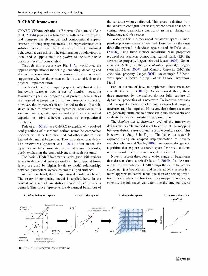
Through this process (see Fig. 1 for workflow), the
applied computational model, e.g., encoding, decoding and
abstract representation of the system, is also assessed,
suggesting whether the chosen model is a suitable fit to the
physical implementation.
To characterise the computing quality of substrates, the
framework searches over a set of metrics measuring
favourable dynamical properties. At present, these metrics
are targeted at properties critical to reservoir computing,
however, the framework is not limited to these. If a sub-
strate is able to exhibit many dynamical behaviours, it is
said to have a greater quality and therefore a increased
capacity to solve different classes of computational
problems.
Dale et al. (2019b) use CHARC to explain why evolved
configurations of disordered carbon nanotube composites
perform well at certain tasks and not others: due to their
limited dynamical behaviour. They also show that delay-
line reservoirs (Appeltant et al. 2011) often match the
dynamics of large simulated recurrent neural networks,
partly explaining the competitiveness of such systems.
The basic CHARC framework is designed with various
levels to define and measure quality. The output of lower
levels are used by higher levels to model relationships
between parameters, dynamics and task performance.
At the base level, the computational model is chosen.
The reservoir computing model is applied here. In the
context of a model, an abstract space of behaviours is
defined. This space represents the dynamical behaviour of
the substrate when configured. This space is distinct from
the substrate configuration space, where small changes in
configuration parameters can result in large changes in
behaviour, and vice versa.
To define this n-dimensional behaviour space, n inde-
pendent property measures are used. Here, we use the same
three-dimensional behaviour space used in Dale et al.
(2019b), using three metrics measuring basic properties
required for reservoir computing: Kernel Rank (KR; the
separation property, Legenstein and Maass 2007), Gener-
alisation Rank (GR; the generalisation property, Legen-
stein and Maass 2007), and Memory Capacity (MC; the
echo state property, Jaeger 2001). An example 3-d beha-
viour space is shown in Step 1 of the CHARC workflow,
Fig. 1.
For an outline of how to implement these measures
consult Dale et al. (2019b). As mentioned there, these
three measures by themselves do not fully capture all
dynamical properties of a reservoir. To improve accuracy
and the quality measure, additional independent property
measures may be required. However, these three measures
are generally sufficient to demonstrate the framework and
evaluate the various substrates proposed here.
The Exploration & Mapping level of the framework
defines the search method used to construct the mapping
between abstract reservoir and substrate configuration. This
is shown as Step 2 in Fig. 1. The behaviour space is
explored using an adapted implementation of novelty
search (Lehman and Stanley 2008), an open-ended genetic
algorithm that explores a search space for novel solutions
until a user-defined termination criterion is met.
Novelty search discovers a wider range of behaviours
than does random search (Dale et al. 2019b) for the same
number of evaluations. CHARC maps the entire behaviour
space, not just boundaries, and hence novelty search is a
more appropriate search technique than explicit optimisa-
tion of some objective function. This mapping process, by
covering the full space, can determine the practical use of
Fig. 1 CHARC framework basic workflow
Reservoir computing quality: connectivity and topology
123
the substrate, or whether the computational model and
configuration method is appropriate.
The use of heuristic search, rather than exhaustive
search, may result in some biases in the results. For
example, the discovered boundaries of the behaviour space
are noisy as they are the most difficult behaviours to find,
therefore they are less frequently discovered. The discov-
ered boundaries also tend to be noisier for systems with
higher quality (see Fig. 4) as the boundaries of lower
quality systems are easier to find in fewer search iterations.
The quality measure used compensates for some noise: if a
behaviour is found, all nearby behaviours are taken to be
possible; CHARC provides a qualitative approximation of
reservoir quality. Also, different reservoir architectures
will have different biases: although some bias is removed
because of the focus on the resulting behaviour space
instead of configuration parameter space, nevertheless a
larger number of configuration parameters will require
greater exploration, and different architectures have dif-
ferent parameter combinations. The fairest way to compare
is the standard approach taken in using evolutionary
algorithms: put the same restriction on the length of each
search. Some architectures may in principal be underex-
plored, but the results indicate that in fact there is rea-
sonably consistent coverage of behaviour space.
The Evaluation level defines the mechanisms to evaluate
quality. This constitutes the final level for measuring
quality. To assess quality, the final behaviour space is
divided into voxels/cells as demonstrated in Step 3 of
Fig. 1. The total number of voxels that are occupied by
behaviours builds an approximation of the dynamical
freedom: how many distinct reservoirs the substrate can
instantiate. This acts as the measure of quality to compare
across systems.
In order to compare fairly across systems the same
number of evaluations and dimensions should be kept, as
well as the same voxel size when measuring quality.
4 Network topology experiments
Simple, regular and deterministic connection topologies
can perform as well as randomly-generated reservoir net-
works on a number of benchmark tasks (Appeltant et al.
2011; Ortın et al. 2015; Rodan and Tino 2010, 2011).
However, the exact role and benefits of complex structures
in reservoir computing is an open question and the full
computing and dynamical limitations of simple topologies
still remains unclear.
4.1 Reservoir model
The dynamics of each reservoir network used in this work
is given by the state update equation:
xðnÞ ¼ ð1� aÞxðn� 1Þ þ af ðbWinuðnÞ þ cWxðn� 1ÞÞð3Þ
where x is the internal state at time-step n, f is the neuron
activation function (a tanh function), u is the input signal,
Win and W are weight matrices giving the connection
weights to inputs and internal neurons respectively. The
parameters a, b and c control the global scaling of: leak
rate, input weights and internal weights. The leak rate
controls the time-scale mismatch between the input and
reservoir dynamics; when a ¼ 1, the previous states do not
leak into the current states. Input scaling (b) affects the
non-linear response of the reservoir and relative effect of
the current input. Internal scaling (c) controls the reservoirs
stability as well as the influence and persistence of the
input; e.g. low values dampen internal activity and increase
response to input, and high values lead to chaotic
behaviour.
The final trained output yðnÞ is given when the reservoir
states xðnÞ are combined with the trained readout weight
matrix Wout:
yðnÞ ¼ WoutxðnÞ ð4Þ
4.2 Topologies
In the experiments here, we use CHARC to investigate the
effect of network topology on quality by evaluating four
simulated reservoir networks: ring, lattice, torus and fully-
connected networks.
The ring topology (Fig. 2a) has the least complexity.
Each node has a single self-connection and a weighted
connection to each of its neighbours to its left and right,
resulting in every node having three adaptable weights in
the internal weight matrix W .
The ring is the simplest network to implement in
physical hardware as the number of connections required is
small. Ring structures with various connection types have
been applied to many reservoir computing systems,
including Simple Cycle Reservoirs (SCR) (Rodan and Tino
2011), DNA reservoirs (deoxyribozyme oscilla-
tors) (Goudarzi et al. 2013), and delay-line reservoirs using
a single non-linear node with a delay line (Appeltant et al.
2011; Paquot et al. 2012).
The lattice topology (Fig. 2b) has greater connection
complexity. With this topology, we define a square grid of
neurons each connected to its nearest neighbours [using its
Moore neighbourhood, as commonly used in cellular
M. Dale et al.
123

automata (Adamatzky 2010)]. Each non-perimeter node
has eight connections to neighbours and one self-connec-
tion, resulting in each node having a maximum of nine
adaptable weights in W .
Lattice networks/models are common in computational
physics, condensed matter physics and beyond, modelling
physical interactions, phase transitions and structure (Lavis
2015). Examples include: discrete lattices like the Ising
model with variables representing magnetic dipole
moments of atomic spins (Brush 1967), and the Gray–Scott
reaction–diffusion model to simulate chemical systems
(Pearson 1993). Physical substrates often have a regular
grid of connections; lattice networks are therefore a real-
istic representation of many physical systems that would be
considered for reservoir computing.
The torus topology (Fig. 2c) is a special case of the
lattice where perimeter nodes are connected to give peri-
odic boundary conditions. Each node has nine adapt-
able weights in W .
Although not a natural topology for physical systems,
turning physical lattices into tori is often relatively simple.
An advantage of the toroidal structure is that it reduces the
signal path distance between perimeter nodes and removes
edge effects, leading to potentially different dynamics at a
minimal cost to connection complexity.
The fully-connected network (Fig. 2d) has no topologi-
cal constraints and has the maximum number of adapt-
able weights: the weight matrix W is fully populated. This
network type is used to benchmark the other topologies.
Due to its large degree-of-freedom in parameter space, this
network likely features the highest quality with respect to
its size. However, fully-connected and random networks
are challenging to implement in physical hardware due
their connection complexity.
Extra complexity can be achieved by increasing the
number of nodes and weights. The number of non-zero
weights in W, as a function of the number of nodes N is
shown in Table 1.
4.3 Experimental parameters
To measure the effect topology has on dynamical beha-
viour and quality, we test each topology across several
network sizes. The network sizes range from 42 ¼ 16 to
202 = 400 nodes. By comparing the different sizes, we can
determine what relationships exist independent of size, and
how relationships scale with network size.
Each network has local (e.g., weights) and global (e.g.,
weight scaling) parameters under manipulation during the
search process. Individual weights in the input layer matrix
Win and the reservoir matrix W are open to mutation and
can be mutated between ½�1; 1�. Global scaling parameters
(a, b and c) are also evolved. For internal weight W scaling
this is a value between [0, 2], and for Win scaling between
½�1; 1�. The leak-rate parameter, controlling the ‘‘leaki-
ness’’ of past states into current states, is restricted between
[0, 1]. Input and internal connectivity of the reservoir
remains constant, depending on the topology. The weight
distribution of Win and W is evolved by a Gaussian
mutation operator.
The output weight matrix Wout for each network is used
only for the memory capacity measure, as both KR and GR
are calculated using only the reservoir states. When the
readout layer Wout is in use, training is carried out using
ridge regression to minimise the difference between the
network output y and the target signal yt.
The CHARC parameters used in the experiments here
are given in Table 2 (see Dale et al. (2019b) for more
Fig. 2 Network topologies under investigation
Table 1 The number of non-zero weights in W, as a function of the
number of nodes N, for the four topologies
Topology No. of weights
Ring 3N
Lattice 9N � 12ffiffiffiffi
Np
þ 4
Torus 9N
Fully-connected N2
Reservoir computing quality: connectivity and topology
123
information). Novelty search is applied using an adapted
version of the steady-state microbial genetic algo-
rithm (Harvey 2009). Using this algorithm, each generation
produces one new individual that is measured for novelty.
The parameters deme size and recombination rate refer
to division of species in the population and percentage of
genes to inherit. The parameters qmin, Kneighbours and qmin
update control the novelty measure.
To produce a good estimate of quality, typically a large
number of novelty search generations are needed. In
practice, the number used depends on computing resources
and time available to evaluate each reservoir. As shown
in Dale et al. (2019b), a rough estimate is typically
achieved with less than a few thousand search generations.
Here, we apply 10,000 generations to create a detailed
picture of each topology and its role.
In all experiments a voxel size of 10 is used for the
quality measure, leading to a voxel volume of 103 for the
3-dimensional behaviour space.
Each novelty search run begins with a random initial
population. 20 separate runs are conducted for each net-
work size and topology, to gather statistics of quality.
4.4 Results
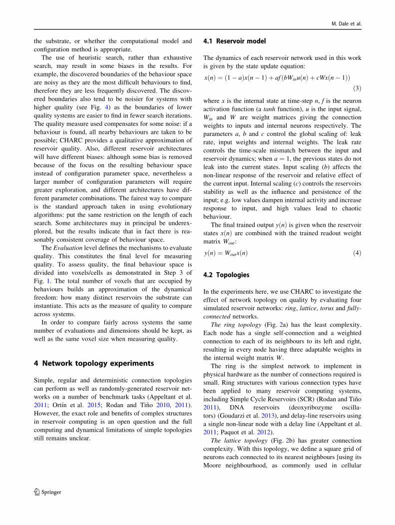
The results for topology and network size are given in
Fig. 3. As network size increases, general network capacity
increases, as expected. The variation (shaded area) between
runs is similar across all the regular topologies. The fully-
connected network tends to have greater variation across
runs than the others, indicating a stronger dependency on
the initial random population.
At a given size (number of nodes) the fully-connected
networks occupy a greater volume of the behaviour space,
possessing a higher quality, than the others, across all sizes.
Also, lattices and tori, with an intermediate number of
connections between rings and fully connected networks,
have intermediate quality. This suggests that, for a fixed
number of nodes, access to more adjustable parameters
(table 1) typically leads to more dynamical behaviours
being available (see §4.4.2 for more on this).
The lattice and torus have similar qualities across all
sizes; however, the difference between them is statistically
significant. Using the non-parametric Wilcoxon rank sum
test, the difference at all sizes (except at N ¼ 324 nodes,
with p ¼ 0:053) is significant at the 95% confidence level
(p\0:05).
The quality of these two topologies is closer to the fully-
connected network than the ring topology. This suggests
there are only a few behaviours the fully-connected can
exhibit that these two topologies cannot.
As size increases, the quality of the ring topology
increases more slowly than the others. To exhibit a similar
quality to the others would require an approximate dou-
bling of ring size.
4.4.1 Behaviour space
To understand what these differences in quality represent,
we visualise the 3-d behaviour space as three projections.
The behaviour space of each topology is shown separately
in Fig. 4a–d, with each network size superimposed onto the
same space. The largest network is placed at the back with
each network size layered in decreasing order towards the
smallest network in the front. Each network size is also
separated by colour.
In Fig. 4, some common patterns exist for each topol-
ogy. Smaller networks are more efficient in terms of
Table 2 Search algorithm parameters for all experiments
Parameter Value
Runs 20
Generations 10,000
Population size 100
Deme size 20%
Mutation rate 10%
Recombination rate 50%
qmin 3
Kneighbours 10
qmin update 100 generations
Voxel size 10
Fig. 3 Mean quality (dots) and standard deviation (shaded area) of all
network topologies, for network sizes N ¼ 42 ¼ 16, 62 ¼ 36,
82 ¼ 64, ..., 202 ¼ 400 nodes (log–log plot)
M. Dale et al.
123
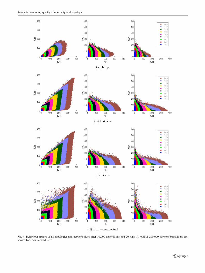
Fig. 4 Behaviour spaces of all topologies and network sizes after 10,000 generations and 20 runs. A total of 200,000 network behaviours are
shown for each network size
Reservoir computing quality: connectivity and topology
123
memory capacity—i.e., possess a larger memory capacity
with respect to network size. As size increases, there is a
considerable drop in efficiency with little gain in overall
capacity.
Sparse areas of the behaviour space highlight chal-
lenging properties to all reservoir structures. For example,
the regions where trade-offs between non-linearity (high
KR), noise (high GR) and memory (high MC) are most
challenging.
The ring topology (Fig. 4a) tends to exhibit more linear
and ordered dynamics characterised by smaller KR and GR
values. As size increases, the space occupied proportional
to network size tends to decrease. This implies that larger
networks struggle more than smaller networks to maintain
non-linearity and input separability.
In terms of non-linear and chaotic dynamics, the lattice
and torus topology (Fig. 4b, c) scale relatively well with
size. Yet, only small gains are made in memory capacity as
size increases; some outliers suggest larger MC values are
possible (longer novelty search runs could discover if this
is the case). This limitation to memory capacity explains
why both topologies have less quality than the fully-con-
nected network. The difference between the torus and the
lattice is due to more consistent high memory capacities
across runs, as seen by the slightly more densely filled
areas in Fig. 4c.
The fully-connected networks (Fig. 4d) do not feature
the same memory limitations as the regular topologies.
This network-type frequently exhibits the more challenging
behaviours, occupying regions with greater trade-offs
between non-linearity and memory. Interestingly, these
networks can occupy areas where noise increases (GR) but
input separation (KR) does not: the upper-left region of the
KR-GR space. This trade-off is more prominent in the
fully-connected network.
4.4.2 Number of connections
Our results above suggest that access to more
adjustable parameters (non-zero elements in W) typically
leads to more dynamical behaviours. Here, we investigate
this further.
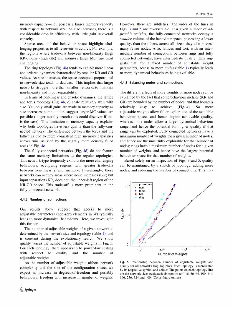
The number of adjustable weights of a given network is
determined by the network size and topology (table 1), and
is constant during the evolutionary search. We show
quality versus the number of adjustable weights in Fig. 5.
For each topology, there appears to be power-law scaling
with respect to quality and the number of
adjustable weights.
As the number of adjustable weights affects network
complexity and the size of the configuration space, we
expect an increase in degrees-of-freedom and possibly
behavioural freedom with increase in number of weights.
However, there are subtleties. The order of the lines in
Figs. 3 and 5 are reversed. So, at a given number of ad-
justable weights, the fully-connected networks occupy a
smaller volume of the behaviour space, possessing a lower
quality, than the others, across all sizes; they also possess
many fewer nodes. Also, lattices and tori, with an inter-
mediate number of connections between rings and fully
connected networks, have intermediate quality. This sug-
gests that, for a fixed number of adjustable weight
parameters, access to more nodes (table 1) typically leads
to more dynamical behaviours being available.
4.4.3 Balancing nodes and connections
The different effects of more weights or more nodes can be
explained by the fact that some behaviour metrics (KR and
GR) are bounded by the number of nodes, and that bound is
relatively easy to achieve (Fig. 4). So more
adjustable weights allow fuller exploration of the available
behaviour space, and hence higher achievable quality,
whereas more nodes allow a larger dynamical behaviour
range, and hence the potential for higher quality if that
range can be exploited. Fully connected networks have a
maximum number of weights for a given number of nodes,
and hence are the most fully explorable for that number of
nodes; rings have a maximum number of nodes for a given
number of weights, and hence have the largest potential
behaviour space for that number of weights.
Based solely on an inspection of Figs. 3 and 5, quality
can be maintained by a switch of topology, adding more
nodes, and reducing the number of connections. This may
Fig. 5 Relationship between number of adjustable weights and
quality for all networks (log–log plot). Each topology is represented
by its respective symbol and colour. The points on each topology line
are the network sizes evaluated: (bottom to top) 16, 36, 64, 100, 144,
196, 256, 324 and 400. (Color figure online)
M. Dale et al.
123

have advantages for manufacturing reservoir substrates.
However, the quality value is a somewhat crude measure,
and may not result in the same collection of behaviours
being produced, for example, different systems with the
same overall quality might not be able to achieve the same
memory capacities (see Fig. 4). The quality measure alone
is not sufficient to guarantee performance on specific tasks:
it gives the overall potential of a substrate, but different
tasks require different values of behavioural metrics (Dale
et al. 2019b) that may lie inside or outside the overall
quality envelope.
5 Network connectivity
Rather than being regular or completely random, many
interesting biological, technological and physical networks
are said to feature small-world topologies or scale-free
properties, exploiting both regular and random struc-
ture (Watts and Strogatz 1998). Networks are considered
small-world when they have a small average path-length
between any two nodes and a high clustering coefficient.
Scale-free networks are characterised by an asymptotic
degree distribution among nodes with large ‘hub’ nodes
typically followed by many smaller-hub nodes.
Both scale-free and small-world topologies have been
applied to Echo State Networks and have shown to
improve performance across certain benchmark tasks
(Deng and Zhang 2007; Kawai et al. 2019). However, the
full range of behaviours exhibited by small-world networks
may be limited. Kawai et al. (2019) find that small-world
reservoirs could not replicate the high linear memory
capacities produced by random and regular networks.
In the experiment in this section, we add a fixed quantity
of evolvable connections to the previous regular structures,
to assess their affect on quality. Adding extra connections
to each topology reduces the signal path length between
distant nodes and alters the degree distribution of nodes in
each topology. We increase the total number of connec-
tions for each topology by setting a randomly-selected
percentage of the non-topological weights—all otherwise
zero-valued entries in W. These new networks, each with
the original topology plus extra random connections, are
then assessed for quality. An example of the ring topology
with extra connections is shown in Fig. 6. 100% additional
connections to any topology results in a fully-connected
network.
Unlike the Watts and Strogatz (1998) small-world
model, which uses a set rewiring probability and set degree
for each node, or the Barabasi and Albert (1999) scale-free
model, which applies preferential attachment, we allow
evolution to rewire and converge to any degree distribu-
tion. The total number of connections remain constant for
each network, as in previous experiments; we fix the per-
centage of extra connections, but allow evolution to chose
which particular connections are used. Whether a new
connection is local or distant and what degree each node
has is left to evolution to decide. As before, mutation can
still change individual weight strengths and global network
parameters.
Figure 7 shows quality versus connectivity of all three
topologies at five network sizes. Figure 7 (left) shows
percentage of additional connections versus quality and
Fig. 7 (right) shows number of weights against quality. The
percentage of connections in both plots begins at 0:05%
and increases to 100% (a fully-connected network). The
mean quality is given over 10 runs with standard deviation
represented by the shaded area. Colours and symbols rep-
resent each topology; lighter and darker shades are used to
separate network sizes.
The lattice and torus increase only marginally in quality
with more connections. The ring exhibits a significant
improvement in quality until it converges with the other
topologies at around 2.5–5%. Depending on network size,
this convergence occurs roughly when, or slightly before,
the number of extra connections equals the number topol-
ogy connections. This symbolises the transition point when
the dominant structure shifts from given topology to
unstructured network.
Fig. 6 Example 64-node
networks with a ring topology
and percentage of additional
connections. Colour represents
strength and sign of weighted
connections. (Color
figure online)
Reservoir computing quality: connectivity and topology
123
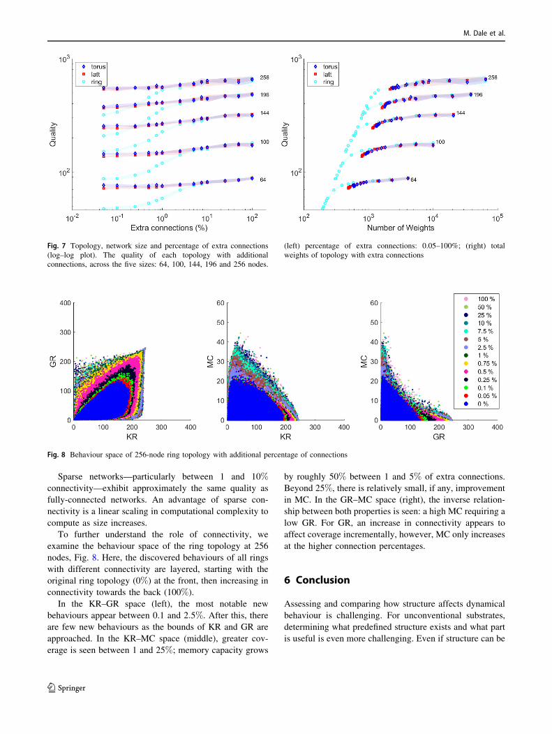
Sparse networks—particularly between 1 and 10%
connectivity—exhibit approximately the same quality as
fully-connected networks. An advantage of sparse con-
nectivity is a linear scaling in computational complexity to
compute as size increases.
To further understand the role of connectivity, we
examine the behaviour space of the ring topology at 256
nodes, Fig. 8. Here, the discovered behaviours of all rings
with different connectivity are layered, starting with the
original ring topology (0%) at the front, then increasing in
connectivity towards the back (100%).
In the KR–GR space (left), the most notable new
behaviours appear between 0.1 and 2:5%. After this, there
are few new behaviours as the bounds of KR and GR are
approached. In the KR–MC space (middle), greater cov-
erage is seen between 1 and 25%; memory capacity grows
by roughly 50% between 1 and 5% of extra connections.
Beyond 25%, there is relatively small, if any, improvement
in MC. In the GR–MC space (right), the inverse relation-
ship between both properties is seen: a high MC requiring a
low GR. For GR, an increase in connectivity appears to
affect coverage incrementally, however, MC only increases
at the higher connection percentages.
6 Conclusion
Assessing and comparing how structure affects dynamical
behaviour is challenging. For unconventional substrates,
determining what predefined structure exists and what part
is useful is even more challenging. Even if structure can be
Fig. 7 Topology, network size and percentage of extra connections
(log–log plot). The quality of each topology with additional
connections, across the five sizes: 64, 100, 144, 196 and 256 nodes.
(left) percentage of extra connections: 0.05–100%; (right) total
weights of topology with extra connections
Fig. 8 Behaviour space of 256-node ring topology with additional percentage of connections
M. Dale et al.
123

decided at creation, what is a suitable or ideal structure is
often limited by physical constraints.
In this work, we have assessed what effect different
structural choices have on quality and how reservoir net-
works might be improved with minimal cost to connec-
tivity. We have applied the task-independent CHARC
framework and used it to directly assess topology and
connectivity and their role on the computing quality of
recurrent neural networks. The results show that networks
with simple topologies and sparse connectivity exhibit
similar quality and behaviours as more complex structures.
However, simple topologies, such as the ring, tend to have
limited behaviour. To overcome this, we propose adding
extra connections to each topology. The results indicate
that quality can increase with extra connections to each
topology, with the ring topology being the most affected.
At around 2.5–5% extra connectivity, each topology tends
to converge towards the same quality across all network
sizes. After this, only minor improvements are found. This
point of convergence typically coincides with the number
of extra connections matching, or outnumbering, the con-
nections required to form each topology.
Our interpretation of these results is that small-world-
like connectivity does not lead to any greater dynamical
behaviour or freedom than fully-connected networks.
However, quality is clearly improved when the topological
constraints are relaxed.
In future work, we will apply these design principles and
methods to create better physical computing substrates.
Acknowledgements This work is part of the SpInspired project,
funded by EPSRC Grant EP/R032823/1. All experiments were carried
out on the University of York’s Super Advanced Research Computing
Cluster (Viking). This is an extended journal version of (Dale et al.
2019a), a UCNC 2019 conference paper, including more network
sizes, longer searches, more runs, and new restrictions to the creation
and alteration of networks. We also include an investigation on the
effects of quality when adding extra random connections to restricted
topologies.
Open Access This article is licensed under a Creative Commons
Attribution 4.0 International License, which permits use, sharing,
adaptation, distribution and reproduction in any medium or format, as
long as you give appropriate credit to the original author(s) and the
source, provide a link to the Creative Commons licence, and indicate
if changes were made. The images or other third party material in this
article are included in the article’s Creative Commons licence, unless
indicated otherwise in a credit line to the material. If material is not
included in the article’s Creative Commons licence and your intended
use is not permitted by statutory regulation or exceeds the permitted
use, you will need to obtain permission directly from the copyright
holder. To view a copy of this licence, visit http://creativecommons.
org/licenses/by/4.0/.
References
Adamatzky A (2010) Game of life cellular automata, vol 1. Springer,
Berlin
Appeltant L, Soriano MC, Van der Sande G, Danckaert J, Massar S,
Dambre J, Schrauwen B, Mirasso CR, Fischer I (2011)
Information processing using a single dynamical node as
complex system. Nat Commun 2:468
Bala A, Ismail I, Ibrahim R, Sait SM (2018) Applications of
metaheuristics in reservoir computing techniques: a review.
IEEE Access 6:58012–58029
Barabasi AL, Albert R (1999) Emergence of scaling in random
networks. Science 286(5439):509–512
Brush SG (1967) History of the Lenz–Ising model. Rev Mod Phys
39(4):883
Crutchfield JP (1994) The calculi of emergence. Phys D
75(1–3):11–54
Dale M, Miller JF, Stepney S, Trefzer MA (2016a) Reservoir
computing in materio: an evaluation of configuration through
evolution. In: 2016 IEEE symposium series on computational
intelligence (SSCI), pp 1–8
Dale M, Miller JF, Stepney S, Trefzer MA (2016b) Evolving carbon
nanotube reservoir computers. In: International conference on
unconventional computation and natural computation. Springer,
pp 49–61
Dale M, Miller JF, Stepney S, Trefzer MA (2017) Reservoir
computing in materio: a computational framework for in materio
computing. In: 2017 international joint conference on neural
networks (IJCNN), pp 2178–2185. https://doi.org/10.1109/
IJCNN.2017.7966119
Dale M, Dewhirst J, O’Keefe S, Sebald A, Stepney S, Trefzer MA
(2019a) The role of structure and complexity on reservoir
computing quality. In: International conference on unconven-
tional computation and natural computation. Springer, pp 52–64
Dale M, Miller JF, Stepney S, Trefzer MA (2019b) A substrate-
independent framework to characterize reservoir computers.
Proc R Soc A 475(2226):20180723
Deng Z, Zhang Y (2007) Collective behavior of a small-world
recurrent neural system with scale-free distribution. IEEE Trans
Neural Netw 18(5):1364–1375
Gallicchio C, Micheli A, Pedrelli L (2017) Deep reservoir computing:
a critical experimental analysis. Neurocomputing 268:87–99
Goudarzi A, Lakin MR, Stefanovic D (2013) DNA reservoir
computing: a novel molecular computing approach. In: Rondelez
Y, Woods D (eds) DNA computing and molecular programming.
Springer, Berlin, pp 76–89
Harvey I (2009) The microbial genetic algorithm. In: European
conference on artificial life. Springer, pp 126–133
Jaeger H (2001) Short term memory in echo state networks. Technical
report GMD 152, GMD-Forschungszentrum Informationstechnik
Kawai Y, Park J, Asada M (2019) A small-world topology enhances
the echo state property and signal propagation in reservoir
computing. Neural Netw 112:15–23
Lavis DA (2015) Equilibrium statistical mechanics of lattice models.
Springer, Berlin
Legenstein R, Maass W (2007) Edge of chaos and prediction of
computational performance for neural circuit models. Neural
Netw 20(3):323–334
Lehman J, Stanley KO (2008) Exploiting open-endedness to solve
problems through the search for novelty. In: ALife XI,
pp 329–336
Lloyd S (2000) Ultimate physical limits to computation. Nature
406(6799):1047
Reservoir computing quality: connectivity and topology
123
Lukosevicius M (2012) A practical guide to applying echo state
networks. In: Orr GB, Muller KR (eds) Neural networks: tricks
of the trade. Springer, Berlin, pp 659–686
Lukosevicius M, Jaeger H (2009) Reservoir computing approaches to
recurrent neural network training. Comput Sci Rev 3(3):127–149
Ortın S, Soriano MC, Pesquera L, Brunner D, San-Martın D, Fischer
I, Mirasso C, Gutierrez J (2015) A unified framework for
reservoir computing and extreme learning machines based on a
single time-delayed neuron. Sci Rep 5:14945
Paquot Y, Duport F, Smerieri A, Dambre J, Schrauwen B, Haelterman
M, Massar S (2012) Optoelectronic reservoir computing. Sci Rep
2:287
Pearson JE (1993) Complex patterns in a simple system. Science
261(5118):189–192
Pugh JK, Soros LB, Stanley KO (2016) Quality diversity: a new
frontier for evolutionary computation. Front Robot AI 3:40
Rodan A, Tino P (2010) Simple deterministically constructed
recurrent neural networks. In: International conference on
intelligent data engineering and automated learning. Springer,
pp 267–274
Rodan A, Tino P (2011) Minimum complexity echo state network.
IEEE Trans Neural Netw 22(1):131–144
Schrauwen B, Verstraeten D, Van Campenhout J (2007) An overview
of reservoir computing: theory, applications and implementa-
tions. In: Proceedings of the 15th European symposium on
artificial neural networks. Citeseer
Stepney S (2008) The neglected pillar of material computation. Phys
D Nonlinear Phenom 237(9):1157–1164
Tanaka G, Yamane T, Heroux JB, Nakane R, Kanazawa N, Takeda S,
Numata H, Nakano D, Hirose A (2019) Recent advances in
physical reservoir computing: a review. Neural Netw
115:100–123
Verstraeten D, Schrauwen B, D’Haene M, Stroobandt D (2007) An
experimental unification of reservoir computing methods. Neural
Netw 20(3):391–403
Watts DJ, Strogatz SH (1998) Collective dynamics of ‘small-world’
networks. Nature 393(6684):440
Publisher’s Note Springer Nature remains neutral with regard to
jurisdictional claims in published maps and institutional affiliations.
M. Dale et al.
123


![A Performance Comparison of Wireless Multi-Hop Network ... · formulation of topology control algorithms to ensure optimum network connectivity [5, 6, 7]. The topology control algorithms](https://static.fdocuments.us/doc/165x107/5f0551777e708231d4125ebb/a-performance-comparison-of-wireless-multi-hop-network-formulation-of-topology.jpg)