RESERVOIR AND SURFACE FACILITIES COUPLED THROUGH PARTIALLY...

RESERVOIR AND SURFACE FACILITIES COUPLED THROUGH PARTIALLY

AND FULLY IMPLICIT APPROACHES

A Thesis

by

MENGDI GAO

Submitted to the Office of Graduate and Professional Studies ofTexas A&M University

in partial fulfillment of the requirements for the degree of

MASTER OF SCIENCE

Chair of Committee, Eduardo GildinCommittee Members, Ding Zhu

Yalchin EfendievHead of Department, Daniel Hill

December 2014

Major Subject: Petroleum Engineering

Copyright 2014 Mengdi Gao

ABSTRACT

During oil production, the change of production states could cause the change

of pressure losses through the production facilities, and consequently result in the

variations of well-boundary-conditions in time. In the de-coupled reservoir simula-

tors, the well boundary condition (i.e. bottom hole pressure) is estimated and fixed.

Therefore, when performing simulations for production prediction, the de-coupled

reservoir simulator would fail to predict the behaviors of the well boundary condi-

tions during production. In this case, a simulator that involves the effects of surface

facilities is necessary when perform production prediction . The implementation of

partially implicit coupling method has faced the issues due to their inaccuracies and

instabilities for complex cases. In this case, the fully implicit coupling is demanded

for such complex. This research explores the concept and implementation of fully

coupling method.

This study focuses on investigating the effects of coupling surface and subsurface

model on production forecast. This production prediction is performed under simple

constraints (i.e. surface production and injection pressures) and various surface

facilities. The results from running the coupled model showed that the bottom

hole pressures of producers are affected by both the gas-oil ratio (GOR) and water

cut. Other surface facility fittings (i.e. chock or valves) and more complex reservoir

description are considered in this project as well.

ii

DEDICATION

To my family and friends

iii

ACKNOWLEDGEMENTS

I take this opportunity to express my profound gratitude and deep regards to my

committee chair, Dr. Gildin and my committee members, Dr. Zhu and Dr. Efendiev

for their exemplary guidance, monitoring and constant encouragement throughout

the course of this thesis. The blessing, help and guidance given by them shall carry

me a long way in the journey of life on which I am about to embark.

I also take this opportunity to express a deep sense of gratitude to my friends

and colleagues and the department faculty and staff for the cordial support, valuable

information and guidance, which helped me in completing this task through various

stages.

Lastly, I thank almighty, my parents and my cousin for their constant encourage-

ment, without which this assignment would not be possible.

iv

NOMENCLATURE

A Cross-section Area

Bw Water Formation Volume Factor

Bo Oil Formation Volume Factor

Bg Gas Formation Volume Factor

D Tubing/Pipe Diameter

fn Non-Slip Friction Factor

f Friction factor

g Gravitational Acceleration

J Jacobian Matrix

J (p) Jacobian Matrix at pth Newton iteration

k Apparent Permeability

krw Relative Permeability to Water

kro Relative Permeability to Oil

krw Relative Permeability to Gas

kx Permeability in X-Direction

ky Permeability in Y-Direction

kz Permeability in Z-Direction

pw Water Phase Pressure

po Oil Phase Pressure

pg Gas Phase Pressure

pcow Oil-Water Capillary Pressure

pcgo Gas-Oil Capillary Pressure

pb Bubble Point Pressure

v

pwf Bottom Hole Flowing Pressure

q̃w Mass Flow Rate of Water Phase

q̃o Mass Flow Rate of Oil Phase

q̃g Mass Flow Rate of Gas Phase

q∗w Volume Flow Rate of Water Phase

q∗o Volume Flow Rate of Oil Phase

q∗g Volume Flow Rate of Gas Phase

Rres Residual Vector of Subsurface Governing Equations

Rtub Residual Vector of Tubing Governing Equations

Rpipe Residual Vector of Surface Pipe Governing Equations

Rrw Residual Vector of Water Conservation Equation in Reservoir Domain

Rro Residual Vector of Oil Conservation Equation in Reservoir Domain

Rrg Residual Vector of Gas Conservation Equation in Reservoir Domain

Rc Residual Vector of Closing Equation in Reservoir Domain

RWw Residual Vector of Water Flow Equation at Bottom Hole

RWo Residual Vector of Oil Flow Equation in Bottom Hole

RWg Residual Vector of Gas Flow Equation in Bottom Hole

RBHP Residual Vector of Pressure Equation in Bottom Hole

Rtw Residual Vector of Water flow Equation in Tubing Domain

Rto Residual Vector of Oil flow Equation in Tubing Domain

Rtg Residual Vector of Gas flow Equation in Tubing Domain

Rtp Residual Vector of Energy Conservation Equation in Tubing Domain

Rpw Residual Vector of Water flow Equation in Surface Pipe Domain

Rpo Residual Vector of Oil flow Equation in Surface Pipe Domain

Rpg Residual Vector of Gas flow Equation in Surface Pipe Domain

vi

Rpp Residual Vector of Energy Conservation Equation in Surface Pipe

Domain

Rbc Residual Vector of Boundary Condition Equation

Rs Solution Gas Oil Ratio

ro Equivalent Gridblock Radius

rw Wellbore Radius

Sw Water Phase Saturation

So Oil Phase Saturation

Sg Gas Phase Saturation

t Time

Un+1 Unknown Vector for Next Timestep

Un+1∗ Updated Unknown Vector for Next Timestep

usl Superficial Velocity of Liquid

um Superficial Velocity of Gas-Liquid Mixture

WI Well Index

x Distance in X-Direction of Cartesian Coordinate

y Distance in Y-Direction of Cartesian Coordinate

z Distance in Z-Direction of Cartesian Coordinate

yl Liquid Holdup

yg Gas Holdup

i, j, k Subscript Specifying the Properties at Location (i, j, k)

i+ 12, j, k Subscript Specifying the Averaged Properties of Location (i, j, k)

and (i+1, j, k)

i, j + 12, k Subscript Specifying the Averaged Properties of Location (i, j, k)

and (i, j+1, k)

vii

i, j, k + 12

Subscript Specifying the Averaged Properties of Location (i, j, k)

and (i, j, k+1)

i− 12, j, k Subscript Specifying the Averaged Properties of Location (i, j, k)

and (i-1, j, k)

i, j − 12, k Subscript Specifying the Averaged Properties of Location (i, j, k)

and (i, j-1, k)

i, j, k − 12

Subscript Specifying the Averaged Properties of Location (i, j, k)

and (i, j, k-1)

n Superscript Indicating the Properties at Current Timestep

n+ 1 Superscript Indicating the Properties at Next Timestep

∂x Solution Vector of Newton Linearization

ρw Water Density

ρo Oil Density

ρg Gas Density

ρL Density of Liquid in Tubing/Pipe segment

µw Water Phase Viscosity

µo Oil Phase Viscosity

µg Gas Phase Viscosity

φ Porosity

λl Non-Slip Liquid Holdup

λw Water Phase Transmissibility

λo Oil Phase Transmissibility

λg Gas Phase Transmissibility

γw Water Phase Hydrostatic Gradient

γo Oil Phase Hydrostatic Gradient

viii

γg Gas Phase Hydrostatic Gradient

θ Inclination Angle

ix

TABLE OF CONTENTS

Page

ABSTRACT . . . . . . . . . . . . . . . . . . . . . . . . . . . . . . . . . . . . ii

DEDICATION . . . . . . . . . . . . . . . . . . . . . . . . . . . . . . . . . . . iii

ACKNOWLEDGEMENTS . . . . . . . . . . . . . . . . . . . . . . . . . . . . iv

NOMENCLATURE . . . . . . . . . . . . . . . . . . . . . . . . . . . . . . . . v

TABLE OF CONTENTS . . . . . . . . . . . . . . . . . . . . . . . . . . . . . x

LIST OF FIGURES . . . . . . . . . . . . . . . . . . . . . . . . . . . . . . . . xiii

LIST OF TABLES . . . . . . . . . . . . . . . . . . . . . . . . . . . . . . . . . xvii

1. INTRODUCTION . . . . . . . . . . . . . . . . . . . . . . . . . . . . . . . 1

1.1 Objectives . . . . . . . . . . . . . . . . . . . . . . . . . . . . . . . . . 31.2 Surface and Subsurface Model Coupling Methods . . . . . . . . . . . 3

1.2.1 Explicit coupling method . . . . . . . . . . . . . . . . . . . . . 41.2.2 Partially implicit coupling method . . . . . . . . . . . . . . . 41.2.3 Fully implicit coupling method . . . . . . . . . . . . . . . . . 4

1.3 Literature Review . . . . . . . . . . . . . . . . . . . . . . . . . . . . . 61.3.1 Advanced well models . . . . . . . . . . . . . . . . . . . . . . 71.3.2 Surface and subsurface coupled models . . . . . . . . . . . . . 8

2. SURFACE AND SUBSURFACE MODELING MECHANISM . . . . . . . 11

2.1 Reservoir Multiphase Modeling . . . . . . . . . . . . . . . . . . . . . 112.1.1 The saturation constraints in reservoir modeling . . . . . . . . 162.1.2 Discretization of conservation equation for water phase . . . . 172.1.3 Discretization of conservation equation for oil phase . . . . . . 212.1.4 Discretization of conservation equation for gas phase . . . . . 22

2.2 Network Multiphase Flow Modeling . . . . . . . . . . . . . . . . . . . 272.2.1 Mass conservation for tubing and pipe . . . . . . . . . . . . . 292.2.2 Momentum conservation for vertical tubing and horizontal pipe 322.2.3 Liquid holdup correlation for vertical tubing . . . . . . . . . . 352.2.4 Liquid holdup correlation for horizontal pipe . . . . . . . . . . 38

x

2.2.5 Flow through choke . . . . . . . . . . . . . . . . . . . . . . . . 43

3. SURFACE AND SUBSURFACE COUPLING MECHANISM . . . . . . . . 46

3.1 Partially Coupling Method . . . . . . . . . . . . . . . . . . . . . . . . 463.1.1 Explicit coupling . . . . . . . . . . . . . . . . . . . . . . . . . 463.1.2 Partially implicit coupling . . . . . . . . . . . . . . . . . . . . 48

3.2 Fully Implicit Coupling Method . . . . . . . . . . . . . . . . . . . . . 503.2.1 Construction of the fully coupling system of equations . . . . . 513.2.2 Newton-Raphson linearization . . . . . . . . . . . . . . . . . . 56

4. EFFECTS OF PARTIALLY IMPLICIT COUPLING FREQUENCY ONPRODUCTION PERFORMANCE . . . . . . . . . . . . . . . . . . . . . . 60

4.1 Field Management System for Coupling . . . . . . . . . . . . . . . . . 604.1.1 Surface management . . . . . . . . . . . . . . . . . . . . . . . 604.1.2 Reservoir management and field management for coupling . . 61

4.2 Descriptions of Surface and Subsurface Models . . . . . . . . . . . . . 644.2.1 Description of reservoir model . . . . . . . . . . . . . . . . . . 654.2.2 Description of production model . . . . . . . . . . . . . . . . . 664.2.3 Description of fluid properties . . . . . . . . . . . . . . . . . . 68

4.3 Case Studies on the Effects of Coupling Frequency on ProductionPerformance . . . . . . . . . . . . . . . . . . . . . . . . . . . . . . . . 684.3.1 Case study with scenario-1 . . . . . . . . . . . . . . . . . . . . 694.3.2 Case study with scenario-2 . . . . . . . . . . . . . . . . . . . . 714.3.3 Case study with scenario-3 . . . . . . . . . . . . . . . . . . . . 734.3.4 Case study with scenario-4 . . . . . . . . . . . . . . . . . . . . 80

4.4 Sensitivity Study and Summary . . . . . . . . . . . . . . . . . . . . . 87

5. EFFECT OF THE SURFACE NETWORK ELEMENTS ON PRODUC-TION PERFORMANCE . . . . . . . . . . . . . . . . . . . . . . . . . . . . 91

5.1 Modification of MATLAB R© Reservoir Simulation Toolbox (MRST) . 915.1.1 Modification of MRST for fully implicit coupling . . . . . . . . 92

5.2 Validation Test of the Modified MRST Fully Coupled Model . . . . . 965.3 The Effect of Coupled Surface Model on Production Performance . . 102

5.3.1 Effects of tubing size . . . . . . . . . . . . . . . . . . . . . . . 1035.3.2 Effects of adding a choke . . . . . . . . . . . . . . . . . . . . . 112

5.4 Performing Fully Coupled Simulator with Realistic Scenario . . . . . 1225.4.1 Description of reservoir model and properties of fluid . . . . . 1225.4.2 Production strategy and facilities’ properties . . . . . . . . . . 1255.4.3 Results and discussions . . . . . . . . . . . . . . . . . . . . . . 126

6. CONCLUSIONS AND RECOMMENDATION . . . . . . . . . . . . . . . . 131

xi

6.1 Summary and Conclusions . . . . . . . . . . . . . . . . . . . . . . . . 1316.2 Future Work . . . . . . . . . . . . . . . . . . . . . . . . . . . . . . . . 133

REFERENCES . . . . . . . . . . . . . . . . . . . . . . . . . . . . . . . . . . . 134

xii

LIST OF FIGURES

FIGURE Page

2.1 Flow across gridblocks in x-direction . . . . . . . . . . . . . . . . . . 17

2.2 Pressure losses in production systems . . . . . . . . . . . . . . . . . . 28

2.3 Flow across tubing segment . . . . . . . . . . . . . . . . . . . . . . . 30

2.4 Flow regime in horizontal pipe (source: Beggs, H.D.5) . . . . . . . . 39

2.5 Flow regime map (based on Beggs, H.D.5) . . . . . . . . . . . . . . . 40

3.1 Flowchart of explicit coupling method . . . . . . . . . . . . . . . . . . 47

3.2 Flowchart of partially implicit coupling . . . . . . . . . . . . . . . . . 49

3.3 Flowchart of fully implicit coupling . . . . . . . . . . . . . . . . . . . 50

3.4 Flowchart of Newton-Raphson method . . . . . . . . . . . . . . . . . 57

4.1 Field management workflow . . . . . . . . . . . . . . . . . . . . . . . 62

4.2 Coupling of field management at the reservoir simulator Newton iter-ation level (source: Adapted from INTERSECT reference manual19) . 63

4.3 Permeability map in x-direction of heterogeneous reservoir model . . 66

4.4 Surface facilities of production systems . . . . . . . . . . . . . . . . . 67

4.5 Oil production of PROD-1 for Scn-1 . . . . . . . . . . . . . . . . . . . 69

4.6 Gas production and bottom hole pressure of PROD-1 for Scn-1 . . . . 70

4.7 Oil and gas production of PROD-1 for Scn-2 . . . . . . . . . . . . . . 72

4.8 Bottom hole pressure of PROD-1 for Scn-2 . . . . . . . . . . . . . . . 73

4.9 Oil production for Scn-3 (PROD-1 and PROD-2) . . . . . . . . . . . 74


xiii

4.11 Gas production for Scn-3 (PROD-1 and PROD-2) . . . . . . . . . . . 76


4.13 Bottom hole pressure for Scn-3 (PROD-1 and PROD-2) . . . . . . . . 78








4.21 NDp of oil and gas for Scn-1 and Scn-2 . . . . . . . . . . . . . . . . . 88

4.22 NDp of oil and gas for Scn-3 and Scn-4 . . . . . . . . . . . . . . . . . 89

5.1 General procedure of MRST fully implicit black-oil solver . . . . . . . 93

5.2 General procedure of modified MRST fully implicit solver forcoupled model . . . . . . . . . . . . . . . . . . . . . . . . . . . . . . . 94

5.3 Jacobian matrix of fully coupled model . . . . . . . . . . . . . . . . . 96

5.4 Comparison of oil production rates from modified MRST and INTER-SECT field management . . . . . . . . . . . . . . . . . . . . . . . . . 98

5.5 Comparison of gas-oil ratio from modified MRST and INTERSECTfield management . . . . . . . . . . . . . . . . . . . . . . . . . . . . . 99

5.6 Comparison of water production rates from modified MRST and IN-TERSECT field management . . . . . . . . . . . . . . . . . . . . . . 100

5.7 Comparison of bottom hole pressure from modified MRST and IN-TERSECT field management . . . . . . . . . . . . . . . . . . . . . . 101

5.8 Injection profiles for investigating the effects of tubing size . . . . . . 103

xiv

5.9 Oil production rates for investigating the effect of tubing size (PROD-1 and PROD-2) . . . . . . . . . . . . . . . . . . . . . . . . . . . . . . 104

5.10 Oil production rates for investigating the effect of tubing size (PROD-3 and PROD-4) . . . . . . . . . . . . . . . . . . . . . . . . . . . . . . 105

5.11 Gas-oil ratio for investigating the effect of tubing size (PROD-1 andPROD-2) . . . . . . . . . . . . . . . . . . . . . . . . . . . . . . . . . 106

5.12 Gas-oil ratio for investigating the effect of tubing size (PROD-3 andPROD-4) . . . . . . . . . . . . . . . . . . . . . . . . . . . . . . . . . 107

5.13 Water production for investigating the effect of tubing size (PROD-1and PROD-2) . . . . . . . . . . . . . . . . . . . . . . . . . . . . . . . 108

5.14 Water production for investigating the effect of tubing size (PROD-3and PROD-4) . . . . . . . . . . . . . . . . . . . . . . . . . . . . . . . 109

5.15 Bottom hole pressure of producers for investigating the effect of tubingsize (PROD-1 and PROD-2) . . . . . . . . . . . . . . . . . . . . . . . 110

5.16 Bottom hole pressure of producers for investigating the effect of tubingsize (PROD-3 and PROD-4) . . . . . . . . . . . . . . . . . . . . . . . 111

5.17 Field water cuts of choked and base models . . . . . . . . . . . . . . . 113

5.18 Injection profiles for comparing base and choked case . . . . . . . . . 114

5.19 Oil production for comparing base and choked case (PROD-1 andPROD-2) . . . . . . . . . . . . . . . . . . . . . . . . . . . . . . . . . 115

5.20 Oil production for comparing base and choked case (PROD-3 andPROD-4) . . . . . . . . . . . . . . . . . . . . . . . . . . . . . . . . . 116

5.21 Gas liquid ratio for comparing base and choke case (PROD-1 andPROD-2) . . . . . . . . . . . . . . . . . . . . . . . . . . . . . . . . . 117

5.22 Gas liquid ratio for comparing base and choke case (PROD-3 andPROD-4) . . . . . . . . . . . . . . . . . . . . . . . . . . . . . . . . . 118

5.23 Bottom hole pressure for comparing base and choke case (PROD-1and PROD-2) . . . . . . . . . . . . . . . . . . . . . . . . . . . . . . . 119

5.24 Bottom hole pressure for comparing base and choke case (PROD-3and PROD-4) . . . . . . . . . . . . . . . . . . . . . . . . . . . . . . . 120

xv

5.25 Reservoir pressure for comparing base and choke case . . . . . . . . . 121

5.26 Cumulative oil production for comparing base and choked case . . . . 121

5.27 Permeability and porosity map of SPE-10 benchmark . . . . . . . . . 124

5.28 Oil production for comparing coupled and non-coupled with SPE-10case . . . . . . . . . . . . . . . . . . . . . . . . . . . . . . . . . . . . 126

5.29 Water production for comparing coupled and non-coupled SPE-10 case 127

5.30 Bottom hole pressure for comparing coupled and non-coupled SPE-10case . . . . . . . . . . . . . . . . . . . . . . . . . . . . . . . . . . . . 127

5.31 Gas-liquid ratio for comparing coupled and non-coupled SPE-10 case 128

5.32 Total cumulative oil production . . . . . . . . . . . . . . . . . . . . . 128

5.33 Iterations of each timestep for comparing the coupled and non-coupledmodel . . . . . . . . . . . . . . . . . . . . . . . . . . . . . . . . . . . 130

xvi

LIST OF TABLES

TABLE Page

2.1 Determination of flow regime (base on: Beggs, H.D.5) . . . . . . . . 41

2.2 Beggs-Brill holdup coefficient (base on: Beggs, H.D.5) . . . . . . . . . 42

2.3 Beggs-Brill holdup coefficient at inclination (base on: Beggs, H.D.5) . 43

2.4 Empirical coefficient for Ros correlation (source from: Economides21) 44

4.1 Descriptions of reservoir models for investigating the effects of couplingfrequency . . . . . . . . . . . . . . . . . . . . . . . . . . . . . . . . . 65

4.2 Properties of production model . . . . . . . . . . . . . . . . . . . . . 68

4.3 Description of fluid properties . . . . . . . . . . . . . . . . . . . . . . 68

5.1 Production strategy and properties of the surface network model . . . 102

5.2 Descriptions of SPE-10 reservoir model . . . . . . . . . . . . . . . . . 123

5.3 Production strategy and facility properties used for coupled case . . . 125

5.4 Production strategy used for non-coupled case . . . . . . . . . . . . . 126

5.5 Summary of iterations and elapsed time . . . . . . . . . . . . . . . . 130

xvii

1. INTRODUCTION

During the life cycle of oil production, pressure losses caused by the surface pro-

duction system could result in a significant impact on the well productivity, especially

for offshore or deep reservoirs. When performing simulations for production predic-

tion and field management, it is then, necessary to implement an integrated modeling

approach, which couples the reservoir with several surface networks. The integrated

model can be realized by applying the coupling methods, in which the surface model

and subsurface model are linked by exchanging control parameters (such as flowing

pressure and flow rate of each phase) at the coupling point (e.g bottom hole).

Based on the time-step convergence criteria and coupling level, several coupling

mechanisms can be used to integrate surface and subsurface models. In general,

they can be classified as explicit, partially implicit and fully implicit. If the obtained

solution is only dependent on the convergence of the reservoir equations, and the

coupling is operated at time-step level, then the method is explicit; the partially

implicit is similar to explicit, the only difference is that the partially implicit coupling

is performed at the Newton iteration-step level. And if the convergence of both

reservoir and surface facility equations is required, then the coupling is called fully

implicit, as it yields completely implicit solutions.

For explicit and partially implicit coupling, the reservoir and surface facilities

are treated as two different domains. As the workflow of explicit coupling relies

on exchanging the boundary parameters at timestep level, this method may exhibit

inaccuracies due to the fact that the boundary conditions are calculated with the

reservoir state at the beginning of the time-step, which cannot represent the Inflow

Performance Relationships (IPR) at the end of the time-step. Partially implicit cou-

1

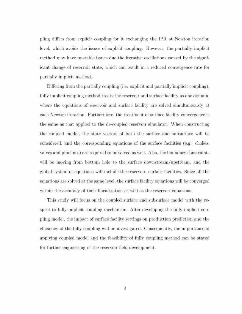
pling differs from explicit coupling for it exchanging the IPR at Newton iteration

level, which avoids the issues of explicit coupling. However, the partially implicit

method may have unstable issues due the iterative oscillations caused by the signif-

icant change of reservoir state, which can result in a reduced convergence rate for

partially implicit method.

Differing from the partially coupling (i.e. explicit and partially implicit coupling),

fully implicit coupling method treats the reservoir and surface facility as one domain,

where the equations of reservoir and surface facility are solved simultaneously at

each Newton iteration. Furthermore, the treatment of surface facility convergence is

the same as that applied to the de-coupled reservoir simulator. When constructing

the coupled model, the state vectors of both the surface and subsurface will be

considered, and the corresponding equations of the surface facilities (e.g. chokes,

valves and pipelines) are required to be solved as well. Also, the boundary constraints

will be moving from bottom hole to the surface downstream/upstream, and the

global system of equations will include the reservoir, surface facilities. Since all the

equations are solved at the same level, the surface facility equations will be converged

within the accuracy of their linearization as well as the reservoir equations.

This study will focus on the coupled surface and subsurface model with the re-

spect to fully implicit coupling mechanism. After developing the fully implicit cou-

pling model, the impact of surface facility settings on production prediction and the

efficiency of the fully coupling will be investigated. Consequently, the importance of

applying coupled model and the feasibility of fully coupling method can be stated

for further engineering of the reservoir field development.

2

1.1 Objectives

When production is controlled by the surface facilities, it is in generally neces-

sary to include the facilities in a full-field model. Thus, the objective of this study

is to construct a fully coupled model and investigate the impact and efficiency of

coupling algorithm to realistic reservoir models. In this study, the results from fully

coupled and non-coupled model will be compared. Furthermore, the computational

costs of various facilities’ settings will be investigated. The main task to achieve

this objective is to construct a fully coupled model with programming software (i.e.

MATLAB R©). Also, the partially implicit coupled powered by commercial software

(i.e. INTERSECT and PIPESIM) will be utilized to test the correctness of our fully

coupled model.

We aim at providing recommendation regarding the usages of the coupling mech-

anisms and computational efforts associated with their implementation. In order

to do that, the additional surface fittings and surface controlling constraints will be

added into the fully coupled model, in order to predict how the otherwise specified

boundary conditions vary in time. And the computational cost of each simulation run

will be stated as well, to demonstrate the efficiency of performing our fully coupled

model.

1.2 Surface and Subsurface Model Coupling Methods

there are various types of coupling methods applied to surface/subsurface coupled

model. Generally, these methods can be classified as three types: explicit, partially

implicit and fully implicit coupling.

3

1.2.1 Explicit coupling method

For the explicit coupling method, the surface and subsurface are treated as two

different domains and the boundary constraint for subsurface (i.e. reservoir) model is

applied explicitly at time-step level. At the beginning of each time-step, the surface

model is performed to calculate the bottom hole pressure (BHP) with the production

rate that obtained from previous time-step, the BHP is then passed to the reservoir

model as the boundary condition, and the reservoir equations are solved with this

boundary condition.

1.2.2 Partially implicit coupling method

Same as explicit coupling, the surface and subsurface are treated differently in

partially implicit coupling method, but the network system is balanced at every

Newton-iteration in each time-step. This method can generate a more accurate so-

lution than explicit coupling. However, the computational speed of implicit coupling

is limited by the time-step size due to its instability occurring when using large

time-step. Also, when the coupling simulations are performed with some commercial

reservoir simulator, the feasibility of implicit coupling is challenged by the compat-

ibility of these commercial reservoir simulator to network simulator. The principles

of implicit and explicit are very similar, as their solution are obtained based the

convergence of reservoir equations.

1.2.3 Fully implicit coupling method

Distinguished from partially coupling (i.e. explicit and implicit coupling), the

fully coupling is trying to get the solution based on the convergence of both the

reservoir and network equations. The nodes of network system are treated as ex-

tended grid blocks of the reservoir domain. Thus, the equations of network (i.e. mass

4

conservation and momentum conservation) is included in the global equation system

and solved at the Newton-iteration level. Since both the reservoir and network sys-

tems are included in the coupled system, the compatibility issue can be avoided by

implementing fully coupling method. Also, the fully implicit coupling can generate

stable solutions. In conventional reservoir model, the system equations are gener-

ally linearized and solved with Newton Raphson method which involves the partial

derivatives of each residual to every unknown variables (such form of derivatives is

called Jacobian matrix). The general structure of Newton linearization (∂X = J−1R)

is shown as:

[ ∂x ] = [ A ]−1[ R ]

Where, the R represents the vector of Residual, while A represents the sub-matrix of

Jacobian matrix, and the ∂x represents the solution of vector of Newton linearization

of the reservoir equations.

The Newton linearization structure of fully coupled model is similar to that of

conventional reservoir model. But the Jacobian matrix will have a different form

due to the additional network system. In this research, the network system will be

further broken down into multi-segment (i.e. vertical tubing) part and the surface

network (i.e. surface pipe) module. Thus, the general Jacobian form of coupled

reservoir and network can be expressed as:

∂Xres

∂Xwb

∂Xpip

=

Ares/res Ares/wb Ares/pip

Awb/res Awb/wb Awb/pip

Apip/res Apip/wb Apip/pip

−1

Rres

Rwb

Rpip

Where, the Rres, Rwb and Rpip represent the residual of each domain (i.e. reservoir,

wellbores and surface pipes). Each element in Jacobian matrix represents a deriva-

5

tive of a residual vector to a variable vector, for instance, Ares/wb represents the

derivative of residual of reservoir equations to the variable vector of multi-segment

part (i.e. ∂Rres

∂Xwb). The vector ∂Xres, ∂Xwb and ∂Xpip represent the solution vectors of

corresponding domains. The Newton linearization will be performed at each New-

ton iteration until the convergences of governing equations occur; In this research,

we study these coupling mechanisms and show how one can access the convergence

criteria for different domains.

1.3 Literature Review

In this section, the development of model coupling will be briefly reviewed. The

evolution of model coupling can be generally classified as two groups: advanced well

modeling and surface/subsurface coupling.

The advanced well modeling has extended the reservoir simulation to a simu-

lation process that considers the flow performance in tubing strings. In this case,

the boundary conditions for reservoir model will be effected by the involvement of

tubing strings, regardless of the surface facility. The advanced well modeling has an

advantage over conventional reservoir model in production prediction, because the

reservoir boundary conditions (production rate or bottom hole flowing pressure) are

usually known for the production prediction case. Thus, it is necessary to move the

boundary constraints to a position where the constraints can be controlled. However,

the advance well modeling is only applicable for the case with simple surface network

constraints, since it fails to represent the production network. When the system in-

volves a complex surface network, the need for a complete surface/subsurface coupled

model becomes necessary.

Many authors have described and implemented the surface/subsurface model in

6

their simulation workflows. Some of these published works are reviewed here.

1.3.1 Advanced well models

In the past years, the implementation of intelligent completion resulted in com-

plex wellbore configurations, and accurately modeling such complexity causes the

requirement of a detailed representation of wellbore composition, rate and pressure

rather than estimated pressure/rate constraints in the conventional reservoir simu-

lation approach.

Holmes et al.1,2 presented an implicit three-phases black-oil model with an implic-

itly coupled wellbore, which is known as advanced well model. The wellbore system

includes four primary variables (i.e. total flow rate, fractional flows of water and gas,

and pressures) in each segment. The global system equations also contains the phase

mass balances and a hydraulic relationship ( i.e. the pressure loss caused by grav-

ity, friction and kinetic energy) for each segment. In this system, the equations for

pressure at the bottom hole was replaced with the boundary condition constraints,

which could be a rate constraints, a bottom-hole flowing pressure constraints and

the tubing-head pressure constraints.

More recent, Stone et al.3 published a more comprehensive model which includes

the compositional and thermal applications. In the work of Stone’s, a multi-segment

and multi-branching wellbore model is fully coupled to a commercial reservoir sim-

ulator. The enhancement of this study is to introduce the energy flow terms into

the equations system which can represent the heat loss along the wellbore segment

due to conduction. As a result, a more accurate volume factor of phases can be

predicted. However, the works described above failed to present a complete surface

facility, both of these systems terminating at tubing-head are unable to represent a

system that includes the surface pipelines/ or a more complex surface network.

7

1.3.2 Surface and subsurface coupled models

Because of the limitation of the advanced well models mentioned above, several

authors have presented methods that simulate the reservoir and the surface facilities

simultaneously. These methods are known as surface/subsurface coupled models. An

early surface/subsurface coupled model was presented within the work of Dempsey4.

This model only simulates a gas/water system, using time-step level explicit coupling.

Since the Hagedorn-Brown5 correlation is used for calculating the pressure drop

through the well tubing, the system can only work for vertical or near-vertical tubing

settings.

Startzman et al.6, then extended Dempsey’s work to a three dimensional black-oil

offshore model coupled with a more complex surface facility. The author implicitly

coupled the surface/subsurface model at the time-step level, and used the same

correlations as Dempsey. Other authors7-8 also presented coupling works involving

different production strategies, such as gas-lift et al.

Schiozer et al.9 presented an novel technique that improves the efficiency of the

coupling method. The authors applied a preconditioner at the beginning of each

time-step, which could provide an estimation of the boundary conditions of the reser-

voir at the new time-step. This technique could increase the equilibrating rate of

well/surface on the first Newton iteration. However, the authors only applied this

new technique to a partially implicit coupled method. Yet the fully coupled method

was concluded as inefficient when applied to complex cases.

Byer et al.10 then extended the application of preconditioner to a fully coupled

model. Rather than using the explicit preconditioning method of Schiozer, a coarse-

grid solution was obtained before each Newton iteration to give an accurate estima-

tion of the reservoir boundary conditions. It is stated that the application of the

8

preconditioning method could reduce the CPU time for certain cases. However, it is

difficult to determine the practicality of this model, as it used a homogeneous no-slip

model for calculating the frictional pressure drop. Although the improved efficiency

was concluded in this work, the CPU time shown in the results are still forbidden as

compared with no coupling methods.

Coat et al.11 developed a comprehensively fully coupled model that involved the

idea of preconditioning. In this model, the equations of the network are solved

simultaneously with the ones of the reservoir. The difference of this model from the

previous works is that it is assumed the network is in steady-state, which avoids the

limitation of transient models in which the time-step size is constrained by the change

of wellbore conditions. Another aspect of this model is that its convergence is based

on reservoir domain, although it had the prior resolution of network/preconditioning,

it still needed a continuous active constraints to obtain an accurate solutions for

network. Also, it is difficult to conclude the impact of network on production from

the results provided, since it focused on discussing the efficiency of this fully coupled

model.

Guyaguler et al.12 proposed a time-step level explicit coupling method. This

method calculated the Inflow Performance Relationships (IPRs) with the near-well

subdomain at the beginning of each coupling period. The IPRs was then set on the

network node coupled to well and used to obtain the rate constraints for reservoir

model. This method substantially reduced the balancing errors and oscillations found

in the previous approaches. However, a noticeable inaccuracy could occur when

applying a large coupling period, and the computational cost may increase when

using small coupling period.

Several authors13-16 presented the coupled model that integrated the commercial

network simulator with some commercial subsurface simulators by using the inter-

9

active field management (FM). Hepgular et al.17 tried to explicitly couple a network

simulator to the commercial software−ECLIPESE with Parallel Virtual Machine

(PVM) interface.

Guyaguler et al.18 integrated the commercial software−PIPESIM with reservoir

simulator aiming to solve the real-world case. And the field management that carries

out the predictive scenarios was introduced in this article. In Guyaguler’s paper, he

also mention that a next-generation simulator is able to couple the separate surface

and subsurface domains with field-management controller (INTERSECT19). How-

ever, details of using the field-management of INTERSECT was not shown in his

paper.

In this chapter, the fundamental concept of coupling surface and subsurface was

introduced. Generally, the coupling methods are classified as explicit, partially im-

plicit and fully implicit based on the convergence criteria and coupling level. Also,

the development and current status of implementation of coupled model in oil in-

dustry was shown, it is concluded that the partially implicit coupling method is

implemented in most practical case, and fully implicit coupling method is currently

not applied into the commercial simulators.

10

2. SURFACE AND SUBSURFACE MODELING MECHANISM

In this chapter, the fundamental formulations and numerical methods that used

in surface/subsurface modeling will be presented. The black oil multiphase reservoir

model will be employed as the subsurface model, where three phases (i.e. water, oil

and gas) fluid flow behavior in porous media will be investigated. The multiphase

flow behavior presented in this chapter is based on the textbook by Ertekin et al.20.

The equations of the network system will also be shown in this section, and the

multiphase flow correlations that used in these equation are based on the textbook

by Economides et al.21.

2.1 Reservoir Multiphase Modeling

This section considers the black oil model for describing the hydrocarbon equilib-

rium in porous media. The formulation of the governing equations that describe this

model include the mass conservation relationship and Darcy’s law. Finite difference

volume approximate procedures are then used for pressure and saturation equations.

In reservoir simulation, the subsurface domain is generally divided into many

grid blocks of small size. Each grid block is treated as a porous medium that has its

own properties (i.e. porosity φ, permeability k, saturation of phases S). The water,

oil and gas phases can flow through the porous media, and consequently perturb

the properties of the media. The phases flow is generally driven by the pressure

differences in between the grid blocks. In black oil model, the densities (i.e. ρw, ρo

and ρg) and viscosity (µw, µo and µg) of phases are used as secondary variables in

the mass conservation equations.

The fundamental phases equation is based on the concept of material mass bal-

11

ance where the mass of fluid accumulation in porous media equals to the difference

between mass of inflow stream and mass of outflow stream, which is shown as:

Massinflow −Massoutflow = Massaccumulation (2.1)

Generally, the fluid flow in porous media obey Darcy’s law, thus the left hand side

(LHS) of Equation 2.1. can be represented by Darcy’s equation, which will give

generalized mass balance in porous media as:

MassF lux′s term = Accumulation term+ Sink/Source term (2.2)

Applying the material mass balance and Darcy’s law to phases will yield the phases

flow equations that is used to describe the states of flow in porous media. In black

oil system, the hydrocarbon components are divided into gas component and oil

component, and there is no mass transfer occurs between the water phase and the

other two phases (i.e. oil and gas). Since there has mass interchange in between

the oil and gas phases, the mass is not conserved within each phase, but the total

mass of each hydrocarbon component has to be conserved. The partial differential

equations of water, oil and gas flow are shown respectively as:

∇[ρwkrwk

µw(∇pw − ρwg∇z)] =

∂(ρwφSw)

∂t+ q̃w. (2.3)

∇[ρokrok

µo(∇po − ρog∇z)] =

∂(ρoφSo)

∂t+ q̃o. (2.4)

∇[ρGokrok

µGo(∇po − ρog∇z) +

ρgkrgk

µg(∇pg − ρgg∇z)] =

∂((ρGoSo + ρgSg)φ)

∂t+ q̃g.

(2.5)

12

For gas equation (2.5), the ρGo indicates the partial density of the gas component

in oil phase. The right hand side of equations (2.3-2.5) is the accumulation term

and external sink/source term (q̃). The LHS is the flux term derived from Darcy’s

equation.

In the porous media, the three phases will jointly fill the void space and the phases

pressure is connected by capillary pressures, which are given by the equations:

Sw + So + Sg = 1 (2.6)

Pcow = Po − Pw, Pcgo = Pg − Po. (2.7)

The water-gas capillary pressure can be given as:

Pcgw = Pcgo − Pcow. (2.8)

Since mass of each hydrocarbon component is not conserved, the dissolved gas-oil

ratio, RS is used to determine the mass fractions of oil and gas components in the

oil phases. The RS is the volume of gas (at the standard conditions) dissolved in a

unit volume of stock tank oil at a specific pressure. The RS is given as:

RS =VGsVOs

(2.9)

where,

VO =WO

ρOand VG =

WG

ρG. (2.10)

where, the WO and WG represent the weights of the oil and gas components, respec-

tively. Then the RS becomes

RS =WGρOWOρG

. (2.11)

13

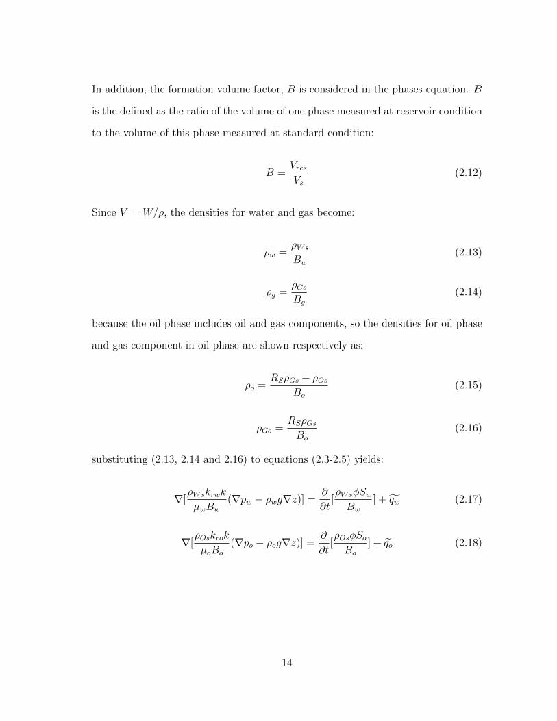
In addition, the formation volume factor, B is considered in the phases equation. B

is the defined as the ratio of the volume of one phase measured at reservoir condition

to the volume of this phase measured at standard condition:

B =VresVs

(2.12)

Since V = W/ρ, the densities for water and gas become:

ρw =ρWs

Bw

(2.13)

ρg =ρGsBg

(2.14)

because the oil phase includes oil and gas components, so the densities for oil phase

and gas component in oil phase are shown respectively as:

ρo =RSρGs + ρOs

Bo

(2.15)

ρGo =RSρGsBo

(2.16)

substituting (2.13, 2.14 and 2.16) to equations (2.3-2.5) yields:

∇[ρWskrwk

µwBw

(∇pw − ρwg∇z)] =∂

∂t[ρWsφSwBw

] + q̃w (2.17)

∇[ρOskrok

µoBo

(∇po − ρog∇z)] =∂

∂t[ρOsφSoBo

] + q̃o (2.18)

14

∇[ρGsRSkrok

µoBo

(∇po − ρog∇z) +ρGskrgk

µgBg

(∇pg − ρgg∇z)]

=∂

∂t[RSρGsφSo

Bo

+ρGsφSgBg

] + q̃oRS + q̃g (2.19)

Defining the Mobility Ratio, λ as the ratio of effective permeability to phase viscosity

and volume factor, then dividing the equations (2.17-2.19) by densities of phases

yields the simplified water, oil and gas conservation equations:

∇[λw(∇pw − ρwg∇z)] =∂

∂t(φSwBw

) + q∗w (2.20)

∇[λo(∇po − ρog∇z)] =∂

∂t(φSoBo

) + q∗o (2.21)

∇[RSλo(∇po − ρog∇z) + λg(∇pg − ρgg∇z)]

=∂

∂t(RSφSoBo

+φSgBg

) + q∗oRS + q∗g (2.22)

The differentiation operator, ∇, indicates the action for taking derivative to the

space vector in three-dimension Cartesian coordinate (i.e. ∂∂x

+ ∂∂y

+ ∂∂y

). Also,

when considering the constraint equations (2.6 and 2.7), the conservation equation

for water, oil and gas phases can be rewritten respectively as:

∂

∂x[λwx(

∂po∂x− ∂pcow

∂x− ρwg

∂z

∂x)] +

∂

∂y[λwy(

∂pw∂y− ∂pcow

∂y− ρwg

∂z

∂y)]

+∂

∂z[λwz(

∂pw∂z− ∂pcow

∂z− ρwg

∂z

∂z)] =

∂

∂t(φSwBw

) + q∗w (2.23)

15

∂

∂x[λox(

∂po∂x− ρog

∂z

∂x)] +

∂

∂y[λoy(

∂po∂y− ρog

∂z

∂y)]

+∂

∂z[λoz(

∂po∂z− ρog

∂z

∂z)] =

∂

∂t[φ(1− Sg − Sw)

Bo

] + q∗o (2.24)

∂

∂x[λoxRS(

∂po∂x− ρog

∂z

∂x)] +

∂

∂y[λoyRS(

∂po∂y− ρog

∂z

∂y)]

+∂

∂z[λoyRS(

∂po∂z− ρog

∂z

∂z)]

+∂

∂x[λgx(

∂pg∂x− ∂pcgo

∂x− ρgg

∂z

∂x)]

+∂

∂y[λgy(

∂pg∂y− ∂pcgo

∂y− ρgg

∂z

∂y)]

+∂

∂z[λgz(

∂pg∂z− ∂pcgo

∂z− ρgg

∂z

∂z)]

=∂

∂t[RSφ(1− Sg − Sw)

Bo

+φSgBg

] +RSq∗o + q∗g (2.25)

2.1.1 The saturation constraints in reservoir modeling

In black oil model, the gas component can exist in both oil phase and gas phase.

When reservoir pressure is higher than the bubble point pressure, the gas component

only exists in oil phase, and the reservoir is regarded as undersaturated, and the

constraint for this condition is:

Sw + So = 1 , Sg = 0 , Rs = 0

and,

po > pb

16

where, pb indicates the bubble point pressure.

When the reservoir pressure is below bubble point pressure, the gas component

starts to vaporize from oil phase, and the free gas phase will present in reservoir

condition, when this occurs, the reservoir is regarded as saturated. The constraints

for saturated reservoir become:

Sw + So + Sg = 1 , Rs > 0

and,

po ≤ pb

2.1.2 Discretization of conservation equation for water phase

To solve the conservation equations provided above, the block-centered finite dif-

ference numerical method is used in this study. First we treat the grid block as a

rectangular cube whose faces are parallel to the Cartesian coordinate axes (see Fig-

ure 2.1). The centroid of the cube is denoted as (x, y, z), and the lengths of cube in

each direction are ∆x,∆y,∆z.

Figure 2.1: Flow across gridblocks in x-direction

17

Referring to Figure 2.1, the mass flux across the interface in x direction can be

expressed as:

(ρux)x−∆x2,y,z , (ρux)x+ ∆x

2,y,z (2.26)

And the pressure differences gradient in x direction are:

pox+∆x+,y,z − pox,y,z∆x+

,pox−∆x−,y,z − pox,y,z

∆x−(2.27)

Applying concepts in the equations (2.26 and 2.27) to the Darcy’s terms in the con-

servation equations yields the discretization of the phase flux in x, y and z directions

for water phase (assuming no potential energy along x, y direction):

∂

∂x[λwx(


∂x− ρwg

∂z

∂x)]

.=

1

∆xi(λwi+ 1

2,j,k

poi+1,j,k − poi,j,k∆x+

i

+ λwi− 12,j,k

poi−1,j,k − poi,j,k∆x−i

) (2.28)

∂

∂y[λwy(

∂po∂y− ∂pcow

∂y− ρwg

∂z

∂y)]

.=

1

∆yi(λwi,j+ 1

2,k

poi,j+1,k − poi,j,k∆y+

i

+ λwi,j− 12,k

poi,j−1,k − poi,j,k∆y−i

) (2.29)

∂

∂z[λwz(

∂pw∂z− ∂pcow

∂z− ρwg

∂z

∂z)]

.=

1

∆zi(λwi,j,k+ 1

2

poi,j,k+1 − poi,j,k∆z+

i

+ λwi,j,k− 12

poi,j,k−1 − poi,j,k∆z−i

− λwi,j,k+ 12γwi,j,k+ 1

2

zi,j,k+1 − zi,j,k∆z+

i

− λwi,j,k− 12γwi,j,k− 1

2

zi,j,k−1 − zi,j,k∆z−i

) (2.30)

where, γ = ρg, the (i, j, k) is the coordinate index that indicates the x, y and z

18

direction respectively. The subscript (i+1, j, k) of water phase pressure, pw indicates

the pressure of the adjacent gridblock in the positive x direction. While (i− 1, j, k)

indicates the properties of adjacent gridblock in negative x direction. The subscript

(i+ 12, j, k) indicates the average property at the interface of two adjacent gridblock

in positive x direction, and the subscript (i− 12, j, k) indicates the properties at the

interface of two adjacent gridblock in negative x direction. Referring to Figure 2.1.,

the distance between the centroids of middle cube and right cube is expressed as

∆x+i , while the distance between middle cube and left cube is expressed as ∆x−i .

The same idea of the subscript is applied to y, z directions.

Combining the equations (2.28-2.30) yields the discretization of Darcy’s term for

water conservation equations:

∂

∂x[λwx(


∂x− ρwg

∂z

∂x)] +

∂

∂y[λwy(

∂po∂y− ∂pcow

∂y− ρwg

∂z

∂y)]

+∂

∂z[λwz(

∂po∂z− ∂pcow

∂z− ρwg

∂z

∂z)]

.=

1

∆xi(λwi+ 1

2,j,k


i

+ λwi− 12,j,k


)

1

∆yi(λwi,j+ 1

2,k


i

+ λwi,j− 12,k


)

1

∆zi(λwi,j,k+ 1

2


i

+ λwi,j,k− 12



2


i


2


) (2.31)

The timescale discretization of accumulation term in water conservation equation

is derived based on the textbook by Ertekin20:

∂

∂t(φSwBw

) = Swn(bw

n+1φ′ + φnbw′)∆pw + (φn+1bw

n+1)∆Sw (2.32)

19

where, bw = 1Bw

, b′w = bwn+1−bwn

pwn+1−pwn , φ′ = φn+1−φnpwn+1−pwn , ∆pw = pwn+1−pwn

∆tand ∆Sw =

Swn+1−Sw

n

∆t.

The superscript, n indicates the properties at the current time-step, while n+ 1

indicates the properties at the next time-step.

In this research, a simplified vertical wellbore model is used. Therefore, the

sink/source term q∗w, can be derived from Peaceman’s equations20, which is shown in

equations (2.33). If the wellbore model involves more complex configurations (e.g.

Fracturing), the Peaceman’s equations will not be applicable.

q∗w = WIw(pwn+1wc − pwf ) (2.33)

where, the subscript, wc indicates the gridblocks where the well is placed. While,

the well index, WIw is defined as:

WIw = −2πkrw

√kxkyh

µwBw[ln( r0rw

) + s](2.34)

where, kx is permeability in x-direction, ky is permeability in y-direction, h is thick-

ness of gridblock, and rw is wellbore radius. The equivalent radius, within which

the pressure is equal to the well-block pressure at steady-state. The formulation for

equivalent wellbore radius is:

r0 = 0.28

√[(kykx

)12 (∆x)2] + [(kx

ky)

12 (∆y)2]

(kykx

)14 + (kx

ky)

14

(2.35)

Combining equations (2.31-2.33) and (2.23) yields the discretization of water conser-

20

vation equation:

1

∆xi(λwi+ 1

2,j,k


i

+ λwi− 12,j,k


)

1

∆yi(λwi,j+ 1

2,k


i

+ λwi,j− 12,k


)

1

∆zi(λwi,j,k+ 1

2


i

+ λwi,j,k− 12



2


i


2


)

= Swn(bw

n+1φ′ + φnbw′)∆pw + (φn+1bw

n+1)∆Sw

+WIw(pwn+1wc − pwf ) (2.36)

2.1.3 Discretization of conservation equation for oil phase

Similarly, the discretization oil flux term can be extended as:

∂

∂x[λox(

∂po∂x− ρog

∂z

∂x)] +

∂

∂y[λoy(

∂po∂y− ρog

∂z

∂y)] +

∂

∂z[λoz(

∂po∂z− ρog

∂z

∂z)]

.=

1

∆xi(λoi+ 1

2,j,k


i

+ λoi− 12,j,k


)

1

∆yi(λoi,j+ 1

2,k


i

+ λoi,j− 12,k


)

1

∆zi(λoi,j,k+ 1

2


i

+ λoi,j,k− 12


− λoi,j,k+ 12γoi,j,k+ 1

2


i

− λoi,j,k− 12γoi,j,k− 1

2


) (2.37)

The oil accumulation term on the RHS is expended regarding to the material

balance:

∂

∂t[φ(1− Sg − Sw)

Bo

] = [(1− Sw − Sg)n(bon+1φ′ + φnb′o)∆po

− (φbo)n+1∆Sw − (φbo)

n+1∆Sg] (2.38)

21

where, bo = 1Bo

, b′o = bon+1−bon

pon+1−pon , φ′ = φon+1−φon

pon+1−pon , ∆po = pon+1−pon∆t

, ∆Sw = Swn+1−Sw

n

∆t

and ∆Sg = Sgn+1−Sg

n

∆t.

The sink/source term for oil phase, qo∗ is expended with Peaceman’s equation:

qo∗ = WIo(pon+1wc − pwf ) (2.39)

where,

WIo = −2πkro

√kxkyh

µoBo[ln( r0rw

) + s](2.40)

Combining the equations (2.37-2.39) and (2.24) yields the discretization formulation

for oil phase conservation:

1

∆xi(λoi+ 1

2,j,k


i

+ λoi− 12,j,k


)

1

∆yi(λoi,j+ 1

2,k


i

+ λoi,j− 12,k


)

1

∆zi(λoi,j,k+ 1

2


i

+ λoi,j,k− 12



2


i


2


)

= [(1− Sw − Sg)n(bon+1φ′ + φnb′o)∆po


n+1∆Sg] +WIo(pon+1wc − pwf ) (2.41)

2.1.4 Discretization of conservation equation for gas phase

For the discretization of gas conservation, the additional terms that represents

the gas components in oil phase are considered, and their formulation in x, y and

22

z-directions are shown respectively as:

∂

∂x[Rsλox(

∂po∂x− γo

∂z

∂x)]

=1

∆xi[(Rsλo)i+ 1

2,j,k


i

+ (Rsλo)i− 12,j,k


] (2.42)

∂

∂y[Rsλoy(

∂po∂y− γo

∂z

∂y)]

=1

∆yi[(Rsλo)i,j+ 1

2,k


i

+ (Rsλo)i,j− 12,k


] (2.43)

∂

∂z[Rsλoz(

∂po∂z− γo

∂z

∂z)]

=1

∆zi[(Rsλo)i,j,k+ 1

2


i

+ (Rsλo)i,j,k− 12


− (Rsλo)i,j,k+ 12γoi,j,k+ 1

2


i

− (Rsλo)i,j,k− 12γoi,j,k− 1

2


] (2.44)

23

Then the gas flux term of conservation is expended as:

∂

∂x[λoxRS(

∂po∂x− ρog

∂z

∂x)] +

∂

∂y[λoyRS(

∂po∂y− ρog

∂z

∂y)]

+∂

∂z[λoyRS(

∂po∂z− ρog

∂z

∂z)]

+∂

∂x[λgx(

∂pg∂x− ∂pcgo

∂x− ρgg

∂z

∂x)]

+∂

∂y[λgy(

∂pg∂y− ∂pcgo

∂y− ρgg

∂z

∂y)]

+∂

∂z[λgz(

∂pg∂z− ∂pcgo

∂z− ρgg

∂z

∂z)]

=1

∆xi[(Rsλo)i+ 1

2,j,k


i



]

+1

∆yi[(Rsλo)i,j+ 1

2,k


i



]

+1


2


i




2


i


2


]

+1

∆xi(λgi+ 1

2,j,k


i

+ λgi− 12,j,k


)

1

∆yi(λgi,j+ 1

2,k


i

+ λgi,j− 12,k


)

1

∆zi(λgi,j,k+ 1

2


i

+ λgi,j,k− 12


− λgi,j,k+ 12γgi,j,k+ 1

2


i

− λgi,j,k− 12γgi,j,k− 1

2


) (2.45)

24

The accumulation term in gas conservation formulation is expended as:

∂

∂t[RSφ(1− Sg − Sw)

Bo

+φSgBg

]

= ∆po{(1− Sw − Sg)n[Rns (bo

n+1φ′ + φnb′o) +R′s(φbo)n+1]

+ Sng (bgn+1φ′ + φnb′g)}

−Rn+1s (boφ)n+1∆Sw

+ [(bgφ)n+1 −Rn+1s (boφ)n+1]∆Sg (2.46)

then, the sink/source term for gas phase can be expended as:

Rsqo ∗+qg∗ = WIg(pgn+1i,j,k − pwf) +Rn+1

s WIo(pgn+1i,j,k − pwf) (2.47)

where, the well index for oil, WIo is already shown in equation (2.48), and the WIg

is:

WIg = −2πkrg

√kxkyh

µgBg[ln( r0rw

) + s](2.48)

Finally, combining equations (2.25) and (2.45-2.47) yields the gas conservation equa-

25

tion:

1

∆xi[(Rsλo)i+ 1

2,j,k


i



]

+1

∆yi[(Rsλo)i,j+ 1

2,k


i



]

+1


2


i




2


i


2


]

+1

∆xi(λgi+ 1

2,j,k


i

+ λgi− 12,j,k


)

1

∆yi(λgi,j+ 1

2,k


i

+ λgi,j− 12,k


)

1

∆zi(λgi,j,k+ 1

2


i

+ λgi,j,k− 12



2


i


2


)

= ∆po{(1− Sw − Sg)n[Rns (bo


+ Sng (bgn+1φ′ + φnb′g)}

−Rn+1s (boφ)n+1∆Sw

+ [(bgφ)n+1 −Rn+1s (boφ)n+1]∆Sg

+WIg(pgn+1i,j,k − pwf) +Rn+1

s WIo(pgn+1i,j,k − pwf) (2.49)

It can be seen that the discretization of the conservation equation for water,

oil and gas phase are complete nonlinear equations. Thus, a linearization method

is required to solve these governing equations. In this study, the Newton-Raphson

method is used to linearize the governing equations. The details of Newton-Raphson

will be discussed in the next chapter.

26

2.2 Network Multiphase Flow Modeling

In black-oil coupled model, the flow in tubing and pipes are generally multiphase

flow. The distribution of different phase in tubing and pipe affects the aspects of

the multiphase flow, such as holdups of phases and pressure gradient throughout the

production system. Thus, it is important to identify the manner where the phases

are distributed. The fundamental theories and formulations that used in this study

are based the textbook by Economides21.

The main task of the network modeling is to determine the pressure losses

throughout the production system (see Figure 2.2), which is the main task when

coupling the surface/subsurface. The distribution of liquid and gas phase has signifi-

cant impacts on the pressure gradient; and the change of pressure in the tubing/pipe

further affects the properties of the fluids, which complicates the production system

modeling. In production system, the pressure loss will occur throughout the entire

surface facilities, and the general formulation for production system is in the form

of:

pwf = psep + ∆pv + ∆pt + ∆pc

where, pwf indicates the bottom hole flowing pressure. ∆pv indicates the pressure

loss caused by the safety valve restriction. The pressure losses through tubing is

indicated by ∆pt. At wellhead, the surface choke is usually used to control the

upstream pressure and fluid flow rate, and the pressure loss across the surface choke

is indicated by ∆pc. Finally, the flowing pressure at separator is indicates by psep.

27

Figure 2.2: Pressure losses in production systems

Usually, the simplified production system does not involve all the surface facilities

that is mentioned above. In this study, the pressure loss across tubing, flowline and

choke will be investigated.

Similar to the reservoir model, the network modeling is operated based on the

concept of material balance. Instead of using gridblocks within reservoir modeling,

the tubing and flowline are divide into several segments, where the phases flow has

only one direction. In each segment, all the phases flow follow the material:

Massinflow −Massoutflow = Massaccumulation

The accumulation is affected by the holdup of each phase. And the partial equations

28

of liquid and gas flow are shown respectively as:

q̃lin − q̃lout = Vsegment∂

∂t(ylρl) (2.50)

(q̃gin − q̃gout) = Vsegment∂

∂t(ygρg) (2.51)

where, Vsegment indicates the volume of each segment of tubing or flowline. The pa-

rameter, yp(p = l, g) indicates the holdup for each phase. In two-phase or multiphase

flow, the lighter phase moves faster than the denser phase. This phenomenon result

in that the in-situ volume fraction of denser phase is greater than the input volume

fraction of this phase, which is called holdup. In multiphase flow, the liquid holdup

is determine by using correlations. Different phases flow correlations are chosen re-

garding to the inclination of flow. The multiphase correlation used in this study will

be discussed late in this section.

2.2.1 Mass conservation for tubing and pipe

Each segment of tubing/pipe is treated as a cylinderical cell, where phases flow

has the same direction (see Figure 2.3). The length of each segment is indicated by

∆xi.

29

Figure 2.3: Flow across tubing segment

Referring to Figure 2.3. the subscript i indicates the properties of fluid within

the segment, while the subscript j indicates the properties of fluid flow at the in-

terface between two adjacent segments. Based on equations (2.50-2.51), the mass

conservation equations for water, oil and gas phase are shown respectively as:

q̃wj − q̃wj+1 = ∆xiAi∂

∂t(ywρWsbw)i (2.52)

q̃oj − q̃oj+1 = ∆xiAi∂

∂t(yoρOsbo)i (2.53)

(q̃gj − q̃gj+1) = ∆xiAi∂

∂t(ygρGsbg +RsyoρGsbo)i (2.54)

where, the mass flow rate q̃ is the flow rate at surface standard conditions. Ai indi-

cates the cross-section area of segment i. The parameters, phase holdup and volume

30

factor are calculated with the segment pressure, pi, where, the segment pressure is

the average value of the pressures at segment interfaces (pi =pj+pj+1

2). Then, taking

the time-scale discretization of the RHS of the tubing conservation equations and

dividing by density yields:

q∗wj − q∗wj+1 =∆xiAi

∆t[(ywbw)n+1

i − (ywbw)ni ] (2.55)

q∗oj − q∗oj+1 =∆xiAi

∆t[(yobo)

n+1i − (yobo)

ni ] (2.56)

(q∗gj − q∗gj+1) =∆xiAi

∆t[(ygbg)

n+1i − (ygbg)

ni + (Rsyobo)

n+1i − (Rsyobo)

ni ] (2.57)

Referring to equations (2.55-2.57), it can be seen that the flow rate change with

time within each timestep, which is called transient flows. Since the timestep in

transient well model is limited by the time scale where the equations of the wellbore

flow are solve with Newton iteration, the computational efficiency will be significantly

reduced for transient wellbore flow. In this study, the flow in wellbore and flowline

is assumed as steady-state, where flows do not change with time at any location in

the well/pipeline system within each timestep, such that:

∆xiAi∆t

[(ywbw)n+1i − (ywbw)ni ] ≈ 0

∆xiAi∆t

[(yobo)n+1i − (yobo)

ni ] ≈ 0

∆xiAi∆t

[(ygbg)n+1i − (ygbg)

ni + (Rsyobo)

n+1i − (Rsyobo)

ni ] ≈ 0

Applying the steady-state flow into the equations (2.55-2.57) yields the finally for-

31

mulation for tubing flow conservation:

q∗wj − q∗wj+1 ≈ 0 (2.58)

q∗oj − q∗oj+1 ≈ 0 (2.59)

(q∗gj − q∗gj+1) +Rs(q∗oj − q∗oj+1) ≈ 0 (2.60)

2.2.2 Momentum conservation for vertical tubing and horizontal pipe

In tubing model, the momentum is conserved in each segment of tubing string,

such that the pressure difference between the two interfaces equals to the fluid pres-

sure loss through the segment. Referring to Figure 2.3., the energy conservation for

one segment can be expressed as:

pi − pi+1 = ∆pPEi + ∆pf i + ∆pacci (2.61)

where, ∆p indicate the pressure loss, the subscript, PE indicates that the pressure

loss is caused by potential energy, the subscript f indicates the pressure loss caused

by friction, and acc stands for the pressure loss due to kinetic energy change. In this

study, the pressure drop caused by kinetic energy change is ignored due to the small

affect compared to pressure drop caused by potential energy and friction. Thus, the

equation (2.61) can be rewritten in pressure gradient form as:

dp

dz= (

dp

dz)pe + (

dp

dz)f , (2.62)

32

where, pi − pi+1 = ∆xidpdz

. And the potential energy term is calculated with:

(dp

dz)pe =

g

gcρ̄sinθ, (2.63)

where, θ = π2

for vertical tubing, and θ = 0 for horizontal pipe. Here ρ̄ is the in-situ

average density in the tubing segment so that:

ρ̄ = ylρl + ygρg, (2.64)

yl =VlVseg

and yl + yg = 1, (2.65)

and yl is the liquid holdup that is calculated with tubing flow correlation. In this

study, the Modified Hagedorn and Brown22 correlation is used to determine the liquid

holdup for vertical tubing, the liquid holdup is determined with Beggs-Brill5 corre-

lation. These multiphase flow correlations will be introduced later in this section.

The friction term is calculated with:

(dp

dz)f =

2fρmu2m

gcD, (2.66)

where, D is the tubing diameter. And ρm is the density of liquid and gas mixture,

which is calculated as:

ρm = ρlλl + ρgλg, (2.67)

where, the λ stands for the input fraction of each phase,

λl =ql

ql + qgand λg = 1− λl

33

for mixture velocity um:

um = usl + usg, (2.68)

where the superficial velocity is

usli =qliAi

and usgi =qgiAi,

and the volumetric flow qli and qgi is the in-situ flow at the conditions of segment i.

the two phase friction factor f is calculated with

f = fnexp(S), (2.69)

where

S =ln(x)

−0.0523 + 3.182ln(x)− 0.8725[ln(x)]2 + 0.01853[ln(x)]4

or

S = ln(2.2x− 1.2) (1 < x < 1.2)

and

x =λlyl2

the no-slip friction factor, fn is based the tubing/pipe relative roughness, ε and

Reynolds number, NRe. According to Economides21, the Chen’s equation is used to

determine no-slip friction factor when Reynolds number is greater than 2100. While

Fanning equation21 is used for the situation where the Reynolds number is less than

34

2100.

Chen equation (NRe > 2100)

1√fn

= −4log{ ε

3.7065− 5.0452

NRe

log[ε1.1098

2.8257+ (

7.149

NRe

)0.8981]} (2.70)

Fanning eqation (NRe < 2100)

fn =16

NRe

(2.71)

where

NRe =ρmumD

µm

and

µm = µlλl + µgλg

Here µl is the viscosity of the oil/water mixture regardless of the emulsion effect.

Also assuming that no slip occurs between oil and water phases, the viscosity of the

liquid mixture is calculated with volume fraction-weighted average as:

µl = (WORρw

WORρw +Boρo)µw + (

BoρoWORρw +Boρo

)µo (2.72)

2.2.3 Liquid holdup correlation for vertical tubing

Liquid holdup in vertical tubing can be determined with several correlations. In

this study, the Modified Hargedorn-Brown22 correlation is implemented for the mul-

tiphase flow in vertical tubing. The modified Hargedorn-Brown correlation is an

35

empirical two-phase flow correlation based on the original Hagedorn-Brown correla-

tion.

The modification of original correlation uses no-slip holdup when the predicted

liquid holdup is less than the no-slip holdup; the Griffith correlation21 is used for

bubble flow in modified Hagedorn-Brown correlation. Bubble flow is the regime

where dispersed bubble of gas phase is in continuous liquid phase, it exists when

λg < LB, where

LB = 1.071− 0.2218(u2m

D) (2.73)

and LB has to be great than or equal to 0.13. Once the flow regime is determined

to be bubble flow, the Griffith correlation is used to determine the liquid holdup

yl = 1− 1

2[1 +

umus−√

(1 +umus

)2 − 4usgus

] (2.74)

where, us is a constant velocity that is equal to 0.24384 m/s. When the flow regime

is determined to be the flow regime rather than bubble flow, the original Hagedorn-

Brown is used to determine the liquid holdup

yl = ψylψ

(2.75)

and

ylψ

= (0.0047 + 1123.32H + 729489.64H2

1 + 1097.1566H + 722153.97H2)0.5 (2.76)

ψ =1.0886− 69.9473B + 2334.3497B2 − 12896.683B3

1− 53.4401B + 1517.9369B2 − 8419.8115B3(2.77)

36

where

H =Nvlp

0.1(CNL)

Nvg0.575p0.1

a ND

(2.78)

B =NvgN

0.380L

N2.14D

(2.79)

and

CNL =0.0019 + 0.0322NL − 0.6642N2

L + 4.9951N3L

1− 10.0147NL + 33.8696N2L + 277.2817N3

L

(2.80)

Nvl = usl 4

√ρlgσ

(2.81)

Nvg = 4

√ρlgσ

(2.82)

ND = D

√ρlg

σ(2.83)

NL = µl 4

√g

ρlσ3(2.84)

where, the surface tension σ is defined as the elastic-like force existing in the surface

of a body, especially a liquid, tending to minimize the area of the surface, caused by

asymmetries in the intermolecular forces between surface molecules.. The SI unit of

surface tension is in Nm

.

37

The advantage of Hagedorn-Brown correlation is that it is able to calculate the

liquid holdup with a set of continuous equations, regardless the identification of the

flow regime. However, this correlation is only applicable for vertical or near-vertical

tubing/pipe. Thus, other correlation has to be applied to the flow in horizontal pipe.

2.2.4 Liquid holdup correlation for horizontal pipe

The Beggs-Brill correlation is advanced in that the Beggs-Brill correlation is ap-

plicable to any flow direction. In this study, the flow regime and liquid holdup

determine is based on the Beggs-Brill correlation. Differing from Hagedorn-Brown

correlation, the Beggs-Brill correlation involves the regime identification, which com-

plicates the modeling of horizontal pipe. Thus, the Beggs-brill is only recommended

for the wellbore or pipe that is not vertical or near vertical.

To introduce the Beggs-Brill correlation, it is necessary to understand the flow

regime in horizontal pipe. The flow regime of horizontal flow is shown in Figure 2.4.

Generally, the flow regime is classified in to three patterns.

Referring from Figure 2.4. the types of flow regimes are defined as: segregated

flows, where the gas and liquid phases are almost separated; intermittent flows, where

the gas and liquid phases exist alternatively; and distributed flows, where the one

phase is dispersed in another phase.

Based on the flow regime, Beggs and Brill gave a flow regime map that involves

the relationship between input liquid holdup, λl and Froude number, NFr (see Figure

2.5). The Froude number is defined as:

NFr =u2m

gD

In the flow regime map, Beggs and Brill also introduced the transitionregime that

38

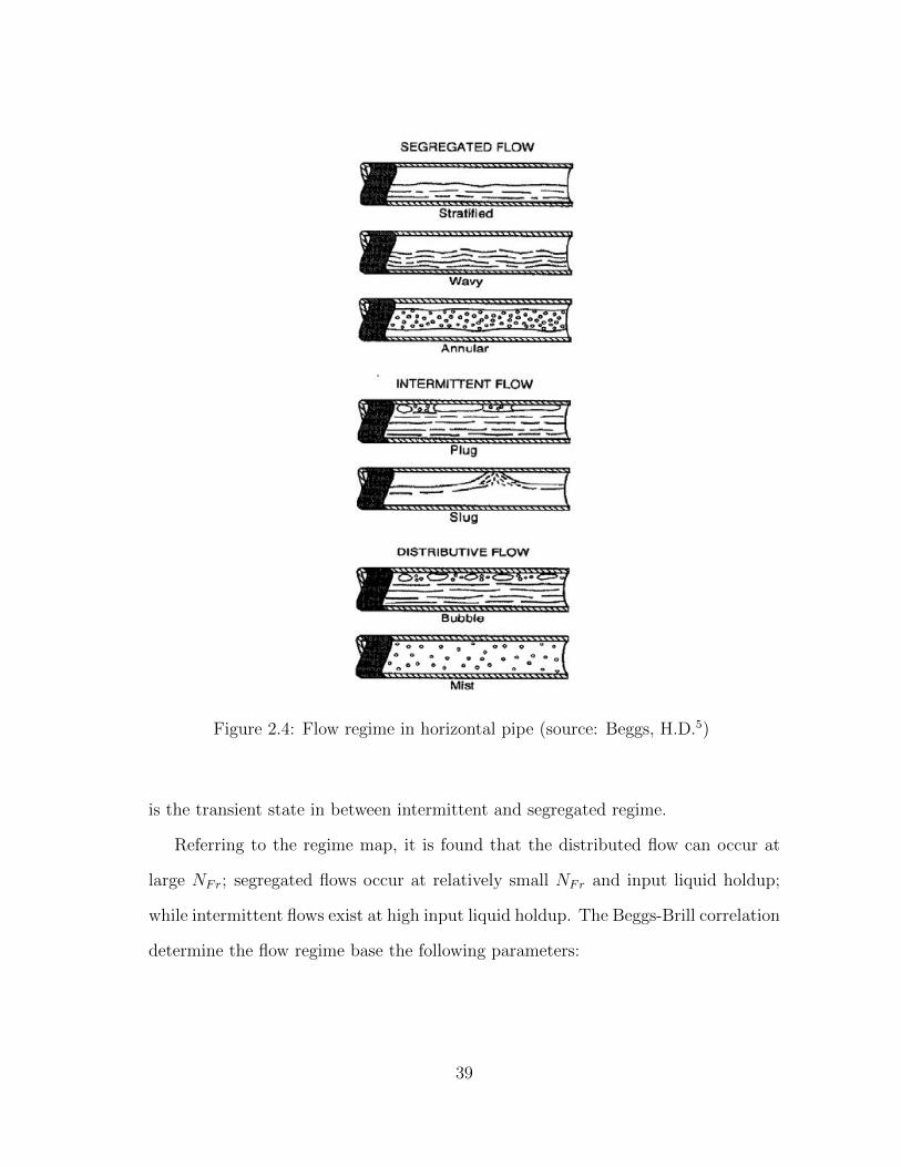
Figure 2.4: Flow regime in horizontal pipe (source: Beggs, H.D.5)

is the transient state in between intermittent and segregated regime.

Referring to the regime map, it is found that the distributed flow can occur at

large NFr; segregated flows occur at relatively small NFr and input liquid holdup;

while intermittent flows exist at high input liquid holdup. The Beggs-Brill correlation

determine the flow regime base the following parameters:

39

Figure 2.5: Flow regime map (based on Beggs, H.D.5)

NFr =u2m

gD(2.85)

λl =uslum

(2.86)

L1 = 316λ0.302l (2.87)

L2 = 0.0009252λ−2.4684l (2.88)

40

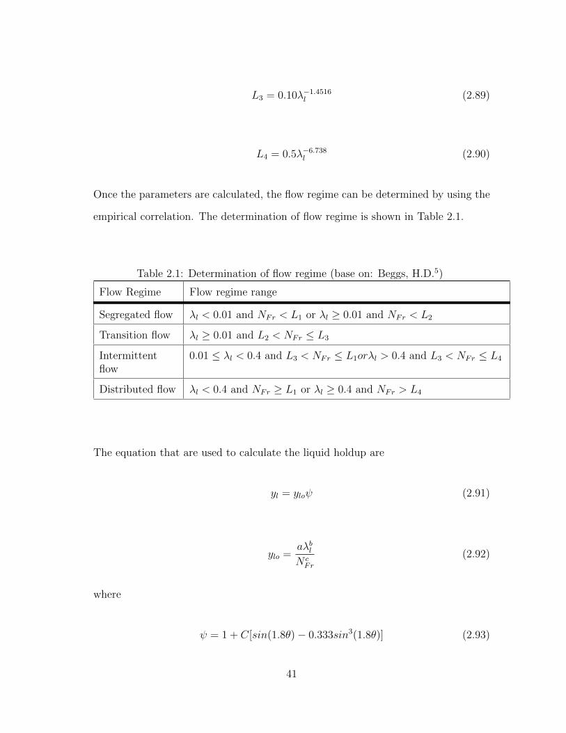
L3 = 0.10λ−1.4516l (2.89)

L4 = 0.5λ−6.738l (2.90)

Once the parameters are calculated, the flow regime can be determined by using the

empirical correlation. The determination of flow regime is shown in Table 2.1.

Table 2.1: Determination of flow regime (base on: Beggs, H.D.5)

Flow Regime Flow regime range

Segregated flow λl < 0.01 and NFr < L1 or λl ≥ 0.01 and NFr < L2

Transition flow λl ≥ 0.01 and L2 < NFr ≤ L3

Intermittentflow

0.01 ≤ λl < 0.4 and L3 < NFr ≤ L1orλl > 0.4 and L3 < NFr ≤ L4

Distributed flow λl < 0.4 and NFr ≥ L1 or λl ≥ 0.4 and NFr > L4

The equation that are used to calculate the liquid holdup are

yl = yloψ (2.91)

ylo =aλblN cFr

(2.92)

where

ψ = 1 + C[sin(1.8θ)− 0.333sin3(1.8θ)] (2.93)

41

where θ is the inclination angle, and

C = (1− λl)ln(dλelNfvlN

gFr) (2.94)

If the flow regime is determined as transition flow, the liquid holdup can be calculated

with both the segregated and intermittent equations and interpolated using following:

yl = Ayl(segregated) +Byl(intermittent) (2.95)

where

A =L3 −NFr

L3 − L2

(2.96)

B = 1− A (2.97)

The coefficient, a, b, c, d, e, f and g used in correlation equation are based on

the flow regime and the value of these holdup coefficients are given in Table 2.2. and

Table 2.3.

Table 2.2: Beggs-Brill holdup coefficient (base on: Beggs, H.D.5)

Flow Regime a b c

Segregated 0.98 0.4846 0.0868

Intermittent 0.845 0.5351 0.0173

Distributed 1.065 0.5824 0.0609

Once the liquid holdup is obtained, the average density and slip friction factor

can be calculated and consequently applied to the pressure gradient calculation.

42

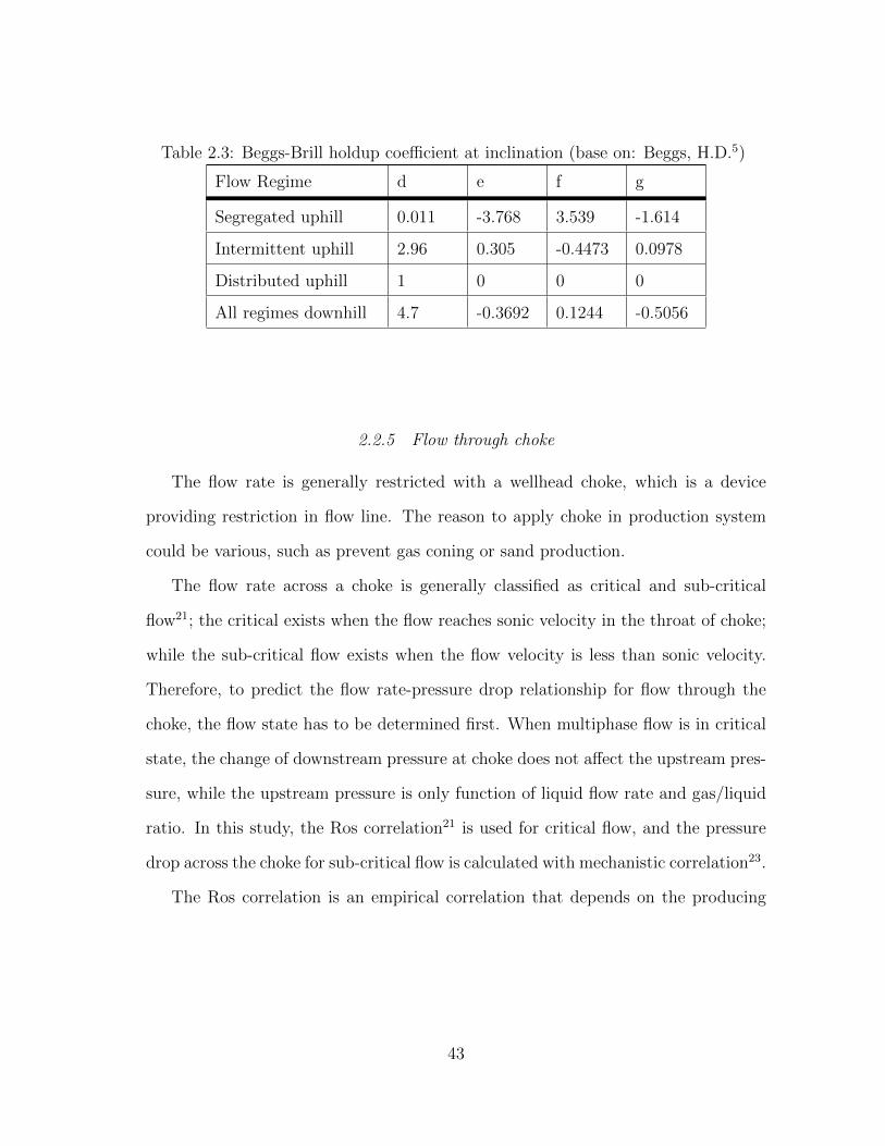
Table 2.3: Beggs-Brill holdup coefficient at inclination (base on: Beggs, H.D.5)

Flow Regime d e f g

Segregated uphill 0.011 -3.768 3.539 -1.614

Intermittent uphill 2.96 0.305 -0.4473 0.0978

Distributed uphill 1 0 0 0

All regimes downhill 4.7 -0.3692 0.1244 -0.5056

2.2.5 Flow through choke

The flow rate is generally restricted with a wellhead choke, which is a device

providing restriction in flow line. The reason to apply choke in production system

could be various, such as prevent gas coning or sand production.

The flow rate across a choke is generally classified as critical and sub-critical

flow21; the critical exists when the flow reaches sonic velocity in the throat of choke;

while the sub-critical flow exists when the flow velocity is less than sonic velocity.

Therefore, to predict the flow rate-pressure drop relationship for flow through the

choke, the flow state has to be determined first. When multiphase flow is in critical

state, the change of downstream pressure at choke does not affect the upstream pres-

sure, while the upstream pressure is only function of liquid flow rate and gas/liquid

ratio. In this study, the Ros correlation21 is used for critical flow, and the pressure

drop across the choke for sub-critical flow is calculated with mechanistic correlation23.

The Ros correlation is an empirical correlation that depends on the producing

43

gas-liquid ratio and liquid rate

pup =Aql(GLR)B

DC64

(2.98)

where D64 is the choke diameter in 64ths of an inch, and the coefficient A, B and C

is given in Table 2.4

Table 2.4: Empirical coefficient for Ros correlation (source from: Economides21)

A B C

17.4 0.5 2.0

The Ros correlation is claimed to be valid for pressure ratio (pdownstream/pupstream)

of 0.7. Therefore, the determination of critical or sub-critical flow is depends on the

pressure ratio in this study, such that the critical flow exists when the 0.7pupstream >

pdownstream, otherwise, the flow is sub-critical. Additionally, the constraint that up-

stream pressure is greater than downstream pressure must be set to guarantee the

flow through the choke.

For sub-critical flow across the choke, the upstream pressure becomes the function

of both the phases flow rates and downstream pressure. The pressure drop across

the choke is calculated with mechanistic correlation23

∆p = λl∆pl + λg∆pg (2.99)

44

and the liquid and gas phase pressure is given by Bernouili’s equation:

∆pl =ρnc

(v

cvl)2 (2.100)

∆pg =ρn2

(v

cvgBg

)2 (2.101)

where the mixture velocity v and no-slip mixture density are calculated with:

v =q

Abeanρn(2.102)

ρn = λlρl + λgρg (2.103)

and λ is the phase flowing fraction at upstream pressure.

In this chapter, the fundamental mechanisms and governing equations of reservoir

and network model are introduced. The governing equations of both models are

mainly based on the material and energy balance. The phase flow correlations (i.e.

Hagedorn-Brown and Beggs-Brill) are employed to determine the liquid holdups for

flow in pipe.

45

3. SURFACE AND SUBSURFACE COUPLING MECHANISM

The main reason of coupling surface and subsurface model is to predict an accu-

rate bottom hole pressure when production constraint is at surface facility. In this

chapter, different coupling methods are presented, and the advantage and disadvan-

tage of each method is discussed as well.

As this study is to investigate and construct the fully coupling model, this sec-

tion summarized the detailed aspects of the fully coupling model. In addition, the

linearization of the governing equations system is presented in order to understand

the concept of the solving system of equations in the fully implicit frame works.

3.1 Partially Coupling Method

As mentioned in chapter one, the partially coupling method involves the explicit

coupling and partially implicit methods. These two method treat the reservoir and

network models as different domains; and solve the equations in the basis of conver-

gence of the reservoir and surface network equations.

3.1.1 Explicit coupling

For explicit coupling, the coupling process is operated at the time-step level.

The well boundary condition (i.e. bottom hole pressure) is calculated with network

model at the beginning of each time-step; the reservoir system is then solved with the

boundary constraint passed from the network model. The flowchart of the explicit

coupling method is shown in Figure 3.1.

46

Figure 3.1: Flowchart of explicit coupling method

Referring to Figure 3.1, the surface and subsurface models are only balanced

at the beginning of each time-step. Therefore, the explicit coupling required few

computational operations. Also since this method treats the reservoir and surface

domain explicitly, the explicit coupling can be accomplished by externally coupling

independent reservoir and network software. The explicit coupling method is em-

ployed in the work of Hepgular et al.17, where the network and reservoir software

are coupled to simulation the overall performance of producing field. However, this

method fails to provide an accurate result due to the fact that the state of reservoir

state cannot represent the state at the end of each time-step.

47

3.1.2 Partially implicit coupling

For partially implicit coupling method, the coupling process is operated at the

Newton iteration level, and the coupling frequency is varied. The general procedure

of partially implicit coupling is:

1. At each Newton iteration, the require for coupling action is determined. If the

coupling action is required for current Newton iteration, the surface model is

solved with the parameters of previous iteration.

2. Once the surface model is converged, the obtained bottom hole pressure (BHP)

is passed to the subsurface model as the boundary constraint.

3. solve the reservoir governing equations with the BHP calculated with surface

model.

4. check the convergence of the reservoir equations.

5. once the reservoir model is converged, process to next time-step.

As the partially implicit coupling method balances the surface and subsurface

model at Newton iteration level, the computational operations is higher than that

of explicit coupling; while the accuracy of the solution is based on the coupling fre-

quency in partially implicit coupling, to this end more coupling or balance frequency

operated will result in more accurate results. When the coupling frequency equals to

one, such that the balancing of surface and subsurface models is only performed at the

first Newton iteration of each time-step, the partially implicit coupling is equivalent

to explicit coupling. Similarly to the explicit coupling, the time-step convergence is

based on only the reservoir equations. However, because of the balancing performed

before solving reservoir equations, the network equations can be converged within

48

the accuracy of their linearizations if the balancing frequency is appropriate. The

flowchart of partially implicit is shown in Figure 3.2. Based on the partially implicit

coupling method, Trick24 coupled a commercial multiphase gas deliverability fore-

casting program and black-oil reservoir simulator, ECLIPSE 100 at Newton iteration

level, and it reported that the coupled model needed sixty minutes to complete one

year forecast.

Figure 3.2: Flowchart of partially implicit coupling

49

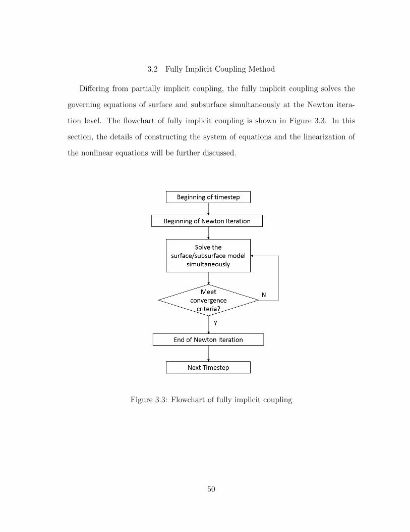
3.2 Fully Implicit Coupling Method

Differing from partially implicit coupling, the fully implicit coupling solves the

governing equations of surface and subsurface simultaneously at the Newton itera-

tion level. The flowchart of fully implicit coupling is shown in Figure 3.3. In this

section, the details of constructing the system of equations and the linearization of

the nonlinear equations will be further discussed.

Figure 3.3: Flowchart of fully implicit coupling

50

3.2.1 Construction of the fully coupling system of equations

In general, the governing equations is contributed by the equations of reservoir,

welbore and surface pipe. These equations are connected by exchanging the material

and momentum parameters (i.e. phases flow rates or pressures) and making sure

these parameters are consistent. Generally, the governing equations are non-linear

function, and one needs to linearize them in order to be able to solve for the unknown

parameters. To this end, one can represent the non-linear equation in terms of the

Residual, R. These residual equations are all based on:

Residual of Discretized Water Conservation Equation

Rrw =1

∆xi(λwi+ 1

2,j,k


i

+ λwi− 12,j,k


)

1

∆yi(λwi,j+ 1

2,k


i

+ λwi,j− 12,k


)

1

∆zi(λwi,j,k+ 1

2


i

+ λwi,j,k− 12



2


i


2


)

− Swn(bwn+1φ′ + φnbw

′)∆pw + (φn+1bwn+1)∆Sw

+ q∗w (3.1)

Residual of Discretized Oil Conservation Equation

51

Rro =1

∆xi(λoi+ 1

2,j,k


i

+ λoi− 12,j,k


)

1

∆yi(λoi,j+ 1

2,k


i

+ λoi,j− 12,k


)

1

∆zi(λoi,j,k+ 1

2


i

+ λoi,j,k− 12



2


i


2


)

− [(1− Sw − Sg)n(bon+1φ′ + φnb′o)∆po


n+1∆Sg] + q∗o (3.2)

Residual of Discretized Gas Conservation Equation

Rrg =1

∆xi[(Rsλo)i+ 1

2,j,k


i



]

+1

∆yi[(Rsλo)i,j+ 1

2,k


i



]

+1


2


i




2


i


2


]

+1

∆xi(λgi+ 1

2,j,k


i

+ λgi− 12,j,k


)

1

∆yi(λgi,j+ 1

2,k


i

+ λgi,j− 12,k


)

1

∆zi(λgi,j,k+ 1

2


i

+ λgi,j,k− 12


52


2


i


2


)

−∆po{(1− Sw − Sg)n[Rns (bo


+ Sng (bgn+1φ′ + φnb′g)} −Rn+1

s (boφ)n+1∆Sw + [(bgφ)n+1 −Rn+1s (boφ)n+1]∆Sg

+ q∗g (3.3)

Residual of Well Water Flow Equation

RWw = q∗w −WIw(pwn+1wc − pwf ) (3.4)

Residual of Well Oil Flow Equation

RWo = q∗o −WIo(pon+1wc − pwf ) (3.5)

Residual of Well Gas Flow Equation

RWg = q∗g −Rn+1s WIo(pg

n+1wc − pwf )−WIg(pg

n+1i,j,k − pwf) (3.6)

Residual of Well Bottom Hole Equation

RBHP = pwf − pt1 (3.7)

where, the pt1 is the pressure at the first node in the tubing. In other words, it is

assumed that the first node of the tubing is located at the bottom hole.

As mentioned in the second chapter, the network system is considered as steady

state, regardless of the changes of phases volumes in time with each segment. There-

fore, the phase flow rate of each node is the same. This implies that the flow rate

53

of each phase equals to the bottom hole phase flow rate, q∗ at surface condition.

Therefore the residue equations for tubing system are:

Residual of Water Conservation in Tubing

Rtw = qtwn+1i − q∗w

n+1 (3.8)

Residual of Oil Conservation in Tubing

Rto = qton+1i − q∗o

n+1 (3.9)

Residual of Gas Conservation in Tubing

Rtg = qtgn+1i − q∗g

n+1 (3.10)

Residual of Energy Conservation in Tubing

Rtp = ptn+1i+1 − ptn+1

i −∆pn+1tj (3.11)

where, the index i indicates the properties at node i, while j indicates the prop-

erties at segment j. The pressure drop though segment j is calculated with energy

conservation equations and Hagedorn-Brown correlation. In addition, the pti at well-

head is calculated with Ros correlation when the flow is critical across the choke,

and the Mechanistic correlation is used when the flow is sub-critical. While the pt

at wellhead equals to the pp (i.e. pressure at node of surface pipe) at wellhead when

there is no choke placed at the wellhead.

The residual equations of surface pipe system is similar to that of tubing system,

54

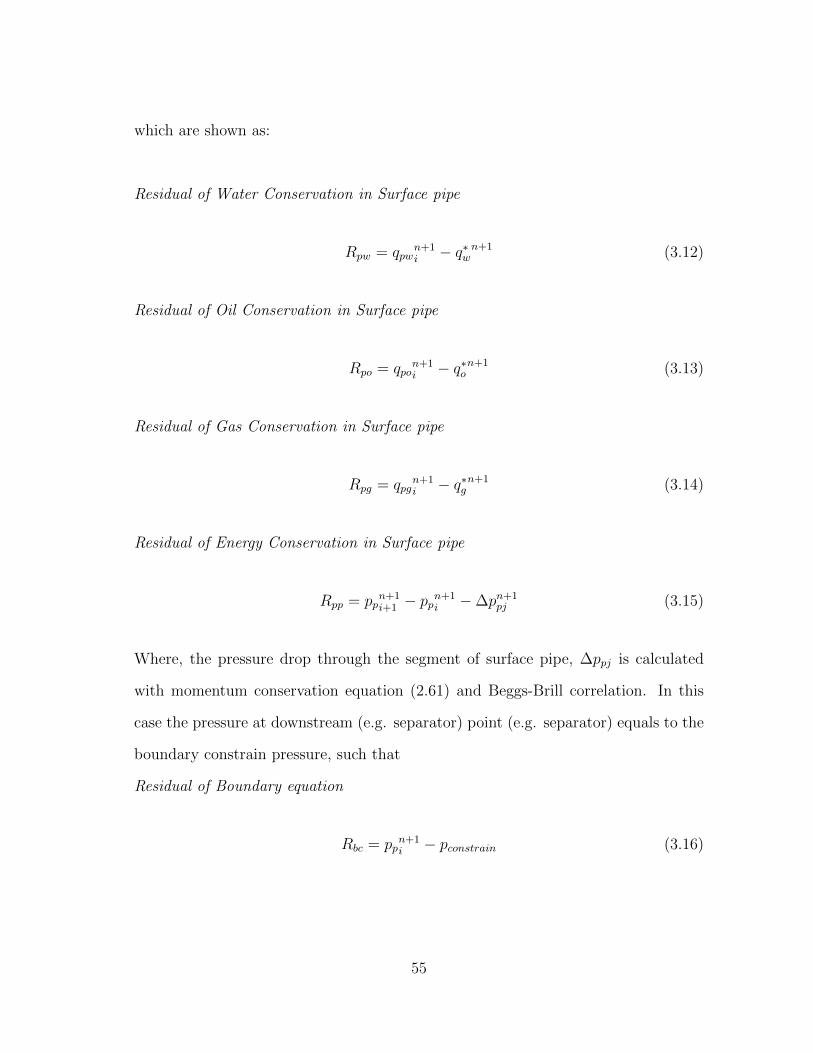
which are shown as:

Residual of Water Conservation in Surface pipe

Rpw = qpwn+1i − q∗w

n+1 (3.12)

Residual of Oil Conservation in Surface pipe

Rpo = qpon+1i − q∗o

n+1 (3.13)

Residual of Gas Conservation in Surface pipe

Rpg = qpgn+1i − q∗g

n+1 (3.14)

Residual of Energy Conservation in Surface pipe

Rpp = ppn+1i+1 − pp

n+1i −∆pn+1

pj (3.15)

Where, the pressure drop through the segment of surface pipe, ∆ppj is calculated

with momentum conservation equation (2.61) and Beggs-Brill correlation. In this

case the pressure at downstream (e.g. separator) point (e.g. separator) equals to the

boundary constrain pressure, such that

Residual of Boundary equation

Rbc = ppn+1i − pconstrain (3.16)

55

3.2.2 Newton-Raphson linearization

Since the fully coupled system equations are nonlinear in terms of the primary

unknown vectors, the lineariztion is performed in order to solve the set of governing

equations. In this study, the Newton-Raphson method is used to linearize and solve

the system equations iteratively. Newton Raphson is a general procedure that can

be applied in many diverse situations. When specialized to the problem of locating a

zero of a real-valued function of a real variable, it is called Newton-Raphson iteration.

If we have a function, f whose zeros are to be determined numerically. Then let r

be a zero of f and let x be an approximation to r. By Taylor’s Theorem:

f(r) = f(x+ h) = f(x) + hf ′(x) +O(h2) = 0

where h = r − x. O(h2) can be ignored if h is small. Therefore, the result is

h = −f(x)/f ′(x). Thus x−f(x)/f ′(x) should be a better approximation to r. Then

the general form for Newton’s method is:

xn+1 = xn −f(xn)

f ′(xn)(n ≥ 0)

In our case, the real-valued function is the residual equations, R(x). The general

scheme of Newton-Raphson is shown in the form of flowchart in Figure 3.4.

56

Figure 3.4: Flowchart of Newton-Raphson method

Referring to Figure 3.4, the Jacobian matrix, J is calculated in order to generate

the linearized system equations for solving the unknown vectors. To understand the

format of Jacobian matrix, the residuals and unknown vectors are defined as:

Residual vectors for reservoir, tubing and surface pipe system

Rres = (Rrw, Rro, Rrg, Rc, RWw, RWo, RWg, RBHP )T

Rtub = (Rtw, Rto, Rtg, Rtp)T

Rpipe = (Rpw, Rpo, Rpg, Rpp, Rbc)T

57

Unknown vectors for reservoir, tubing and surface pipe system

Ures = (pres, Sw, Sg, Rs, qw, qo, qg, pwf )T

Utub = (ptub, qtw, qto, qtg)T

Upipe = (ppipe, qpw, qpo, qpg)T

Then the Jacobian matrix can be formed as

J =∂R

∂U=

∂Rres

∂Ures

∂Rres

∂Utub

∂Rres

∂Upipe

∂Rtub

∂Ures

∂Rtub

∂Utub

∂Rtub

∂Upipe

∂Rpipe

∂Ures

∂Rpipe

∂Utub

∂Rpipe

∂Upipe

(3.17)

After obtain the Jacobian of coupled system, the current state/unknown vector is

updated with Newton-Raphson iteration, which is shown:

δUp = (Jp)−1(−Rp) (3.18)

Up+1 = Up + δUp (3.19)

The Newton Raphson iteration is performed continuously until the residuals of

governing equations are converged. The identification of convergence depends on

whether the residuals equals to zero. In practical, the iteration will stop when all

the norms of residuals are smaller than the set tolerance values, while the tolerance

values may vary for different governing equations.

In this chapter, the detailed scheme of each coupling method is presented, and

it is found that the convergences of both explicit and partially implicit is based on

58

the reservoir governing equations, while the convergence of fully implicit coupling

is determine in the basis of reservoir and surface facility governing equations. Also,

the residual equations of fully coupled system is presented in this chapter; and the

linearization of residuals in a form of Jacobian matrix is presented as well. The

Newton-Raphson iteration is then introduced in order to explain the process of solv-

ing the fully coupled system.

59

4. EFFECTS OF PARTIALLY IMPLICIT COUPLING FREQUENCY ON

PRODUCTION PERFORMANCE

In this chapter, the impacts of coupling frequency on production performance

under different reservoir descriptions will be investigated. Here, we couple the com-

mercial reservoir and network simulators in a partially implicit fashion to access the

production performance forecast. Consequently, the results and computational costs

of the each production performance will be presented.

4.1 Field Management System for Coupling

This section gives a general overview of the field management that is used in this

study. The Field Management includes the reservoir and surface models as well as

production strategy for coupling the surface/subsurface model. The general process

of constructing a partially-implicit coupled model will also be presented.

4.1.1 Surface management

The surface management is realized with the PIPESIM23 Network model; PIPESIM

is a commercial network simulator developed by Schlumberger. In this study, the

main task of using PIPESIM is to calculate the pressure drop throughout the sur-

face system and generate the Inflow Performance Relationship (IPR) for coupling

purpose.

In the Field Management system, the data of PIPESIM model is input in the

”casenam.pst” file format. The PST. file contains the keyword that specifies each

surface facility (e.g. the tubing, surface flowline and sink). In our case study, both the

tubing and pipes have ten nodes, of which the location and temperature is specified.

60

Since the constructed surface model is isothermal, the temperatures at all nodes is

the same as the temperature in the reservoir. The correlations used for calculating

the pressure gradient in vertical flow is the modified Hagedorn-Brown, which is shown

in the previous chapters. For horizontal flow, the Beggs-Brill correlation is used to

calculate the pressure gradient. The vertical or horizontal flow is determined in basis

of the inclination angle. To this end, if the inclination angle is greater than forty-five

degree, the flow is treated as vertical flow, otherwise, the flow is treated as horizontal

flow.

4.1.2 Reservoir management and field management for coupling

The INTERSECT19 reservoir model is used as the subsurface modeling tool.

INTERSECT is the next-generation reservoir simulator developed by Sclumberger.

In order to design the scheduling and control of the oilfield production operations,

the INTERSECT Field Management is used in this study.

The Field Management system is generated by adding user edits to the file called

”casename fm edits.ixf”; and it provides a comprehensive framework and set of tools

with which to build a working operational model of the oilfield. This model captures

all the operational constraints and complex operating logic required to manage the

asset. As the model is moved through time, different production strategies may be

explored using reservoir simulation workflows. Different predictive scenarios may

be evaluated to assist in field development planning, surface facility design, and in

the optimization of revenue from the asset. The work-flow of INTERSECT Field

Management is shown in Figure 4.1.

61

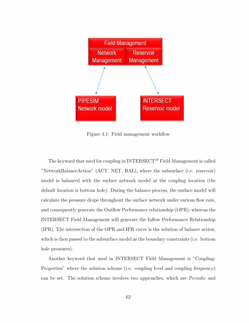
Figure 4.1: Field management workflow

The keyword that used for coupling in INTERSECT19 Field Management is called

”NetworkBalanceAction” (ACT NET BAL), where the subsurface (i.e. reservoir)

model is balanced with the surface network model at the coupling location (the

default location is bottom hole). During the balance process, the surface model will

calculate the pressure drops throughout the surface network under various flow rate,

and consequently generate the Outflow Performance relationship (OPR); whereas the

INTERSECT Field Management will generate the Inflow Performance Relationship

(IPR). The intersection of the OPR and IPR curve is the solution of balance action,

which is then passed to the subsurface model as the boundary constraints (i.e. bottom

hole pressures).

Another keyword that used in INTERSECT Field Management is ”Coupling-

Properties” where the solution scheme (i.e. coupling level and coupling frequency)

can be set. The solution scheme involves two approaches, which are Periodic and

62

Iteratively Lagged. In the Periodic solution method, the coupling action is performed

once at the beginning of every defined period (e.g. 0, 30, 60 days and so on.), which

means the coupled is taken place at the timestep level. The periodic solution method

results in a looser coupling, and produces shorter run times.

In the Iteratively Lagged solution method, the coupling action is performed at

defined number (Nc) of Newton Iterations within every timestep, the Nc is called

coupling frequency. If the reservoir simulator converge within the first Nc iterations,

then the strategy will be executed fewer times. While if the more Newton iterations

are required for convergence of the reservoir model, then bottom hole pressure targets

will be fixed to those determined by the Field Management system for the remainder

of the reservoir iterations. These iterations are referred to as non-coupled Newton

iterations. An example of Iteratively Lagged solution is displayed in Figure 4.2,

where the Nc equals to 3.

Figure 4.2: Coupling of field management at the reservoir simulator Newton iteration

level (source: Adapted from INTERSECT reference manual19)

63

Referring to Figure 4.2, the reservoir simulator cannot converge after 3 iterations

at time step t1, therefore the rest iterations are treated as non-coupled. While at

time step t3 the reservoir simulator converged after two iterations, hence the strategy

is not set by Field Management after the second iteration.

The advantage of Using INTERSECT Field Management is that it can externally

couple the reservoir and network simulator. Other coupling tools (e.g. ECLIPSE net-

work option) usually use the VLP tables obtained from the surface production model

in order to generate the IPR. However, this method may fail to couple the surface

and subsurface model when the current states of parameters exceed the limitation

of the VLP table. Since the Field Management enables the reservoir simulator to

couple with the surface production simulator in a seamless fashion, instead of esti-

mating the control constraints with a pre-generated VLP table, the coupling with

Field Management is capable to access all the states of parameters during the simu-

lation run. However, the INTERSECT Field Management currently fail to support

the injection networks, therefore only the production networks are coupled with the

reservoir model in the study of this chapter. The impact of the injection networks

on the production performance will be investigated with the fully implicitly coupled

model in next chapter.

4.2 Descriptions of Surface and Subsurface Models

This section focuses on the investigation of the effect of the coupling frequency

on the production performance under different reservoir descriptions. The coupled

model is preformed with the partially implicit coupling method. The descriptions of

the reservoir and production properties will be shown below.

64

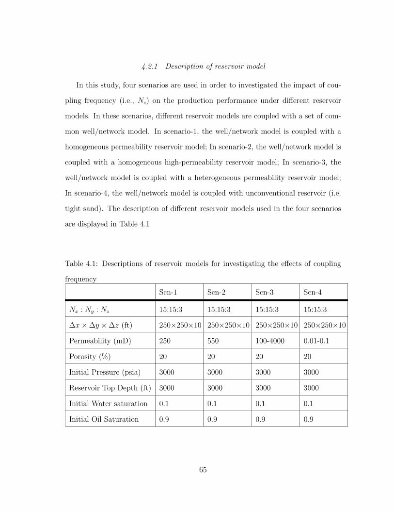
4.2.1 Description of reservoir model

In this study, four scenarios are used in order to investigated the impact of cou-

pling frequency (i.e., Nc) on the production performance under different reservoir

models. In these scenarios, different reservoir models are coupled with a set of com-

mon well/network model. In scenario-1, the well/network model is coupled with a

homogeneous permeability reservoir model; In scenario-2, the well/network model is

coupled with a homogeneous high-permeability reservoir model; In scenario-3, the

well/network model is coupled with a heterogeneous permeability reservoir model;

In scenario-4, the well/network model is coupled with unconventional reservoir (i.e.

tight sand). The description of different reservoir models used in the four scenarios

are displayed in Table 4.1

Table 4.1: Descriptions of reservoir models for investigating the effects of coupling

frequency

Scn-1 Scn-2 Scn-3 Scn-4

Nx : Ny : Nz 15:15:3 15:15:3 15:15:3 15:15:3

∆x×∆y ×∆z (ft) 250×250×10 250×250×10 250×250×10 250×250×10

Permeability (mD) 250 550 100-4000 0.01-0.1

Porosity (%) 20 20 20 20

Initial Pressure (psia) 3000 3000 3000 3000

Reservoir Top Depth (ft) 3000 3000 3000 3000

Initial Water saturation 0.1 0.1 0.1 0.1

Initial Oil Saturation 0.9 0.9 0.9 0.9

65

Since the permeability maps of the heterogeneous models (Scn-3 and Scn-4) can-

not be displayed in the table form, the distribution of the permeability in x-direction

of the reservoir is shown in Figure 4.3. The permeability range from 100-4000 mD

with a high permeable channel located in the northwest part of the reservoir. And

the average of the permeability is around 200 mD, while the ratio of permeability

(vertical direction to horizontal direction) is 0.1.

Figure 4.3: Permeability map in x-direction of heterogeneous reservoir model

4.2.2 Description of production model

The production strategy used in this study is five-spot water flooding with one

injection well placed in the middle of the reservoir and four producers located at

66

the corners of the reservoir, and the example of the production system is shown in

Figure 4.4. The properties of these four production systems are identical, which are

displayed in the Table 4.2. The production network of each producer consists of

a horizontal pipeline and a constant pressure separator is set at the end of surface

pipeline. Since the injection well is not coupled in this phase of study, the properties

of injection well is not provided.

Figure 4.4: Surface facilities of production systems

67

Table 4.2: Properties of production model

Production System Properties Value Unit

Production Tubing ID 3 in

production Tubing Length 3005 ft

Surface Pipe ID 3 in

Downstream Production pressure 300 psia

Bottom Hole pressure of Injection well 3700 psia

4.2.3 Description of fluid properties

The fluid that used in this study is lived-oil, such that there will be three phases

to be considered in the coupled the model. The properties of the fluids that used is

displayed in the Table 4.3. The oil is saturated at the pressure of 4014.7 psia.

Table 4.3: Description of fluid properties

Fluid Properties Value Unit

Oil Density 48.33 API

Gas Specific Gravity 0.819

Water Specific Gravity 1.038

Solution GOR 1.6 MSCF/STB

4.3 Case Studies on the Effects of Coupling Frequency on Production Performance

In order to investigation the effect of coupling on production performance, each

scenario described above is performed with three different coupling frequency (Nc =

68

1, 3, 15).

4.3.1 Case study with scenario-1

In this case study, the predictive results of oil production, gas production and

bottom hole pressure under different coupling frequency will be displayed. In ho-

mogeneous permeable reservoir, the production states are identical for all four wells,

therefore, only the production forecast of PROD-1 is displayed and discussed in the

case study of homogeneous reservoir models.

The oil production, gas production, and bottom hole pressure of PROD-1 are

shown in Figures 4.5-4.6, where the blue curve, green curve and red curve represent

the production profiles under the coupling frequency of 1, 3 and 15, respectively.

The total simulation time is 1100 days.

Figure 4.5: Oil production of PROD-1 for Scn-1

69

Figure 4.6: Gas production and bottom hole pressure of PROD-1 for Scn-1

70

Inferred from the results provided above, it can be observed that the difference

between the production profiles of Nc=3 and that of Nc=15 is not significant, while

the production profile of Nc=1 significantly differs from that of the other two. This

differences indicate that the balancing between the reservoir and production model is

not complete when the coupling frequency equals to one, and the control parameters

(boundary condition) calculated with the production model cannot represent the

control parameters at the end of the time-step. In such manner, the results obtained

with this coupling frequency will have relative large errors. In addition, an oscillation

occurred at the 59th iteration. This can be explained as that the reservoir model failed

to obtain the solution within the default iterations by using the boundary conditions

passed from well/network model.


Similar to the Scenario-1, the predictive results of oil production, gas production

and bottom hole pressure of Scenario-2 is displayed in Figure 4.7-4.8.

71

Figure 4.7: Oil and gas production of PROD-1 for Scn-2

72

Figure 4.8: Bottom hole pressure of PROD-1 for Scn-2

By observing the results above, we concluded that the difference of production

profile between different coupling frequency in high-permeable reservoirs are larger

than that in low permeable reservoir, regardless of the oscillation occurred in the

case of low-permeable reservoir.

One of the possible reason is that the mobility ratio in high-permeable reservoir

is higher than that in the low-permeable reservoir referring to Peaceman’s equation

(see Equation 2.33). Therefore, the production rate is more sensitive to the change

of flowing pressure at bottom hole.


For the heterogeneous permeability reservoir model, the production profiles of

four producers are located at different permeability zone. Referring to Figure 4.3,

73

it can be observed that PROD-1 is located at the high permeability zone, while

the other three producers is placed at the low permeability zones. Similarly to the

previous cases, the production profiles for Scenario-3 are shown in Figure 4.9-4.14

Figure 4.9: Oil production for Scn-3 (PROD-1 and PROD-2)

74


75

Figure 4.11: Gas production for Scn-3 (PROD-1 and PROD-2)

76


77

Figure 4.13: Bottom hole pressure for Scn-3 (PROD-1 and PROD-2)

78


Referring to the results above, it can be seen that the differences in oil and

79

gas production performance due to the various coupling frequencies are not obvious

compared to the production profiles of the homogeneous reservoir. This can be

explained as the change of pressure and flow rate in the heterogeneous permeability

case is not significant as those in the homogeneous permeability case, therefore, fewer

coupling frequency is needed to obtain the accurate parameters at coupling point.


In general, the permeability of unconventional reservoir is extremely low, which

will result in low production rates and relatively stable production behavior.

This case study will investigate the impacts of the coupling frequency on the

production performance under unconventional reservoir. The permeability of the

unconventional reservoir model ranges from 0.01 to 0.1 mD, and the permeability

map is simular to the one of Scn-3. Figure 4.15-4.20 show the production profiles of

Scn-4.

80


81


82


83


84


85


86

Referring to the results shown above, it can be seen that the oil/gas production

rates from tight oil reservoir is very low, and there is no obvious drop in production

rate. This can imply that the reservoir pressure is kept almost constant during the

production. Since there is no significant variations of production profiles in time, the

Filed-Management needed low coupling frequency to complete the coupling/balance

action. Therefore, the differences in production profiles under different coupling

frequency are not obvious. It can be concluded that the tight oil reservoir is not

sensitive to the coupling frequency.

4.4 Sensitivity Study and Summary

In this section, we investigated the impacts of various coupling frequencies on the

production profiles under different descriptions of reservoir models. The quantified

change in cumulative production due to various coupling frequency is analyzed in

this section.

Since the total production differs for different descriptions of reservoir model, it is

difficult to compare the their changes directly. Therefore, we used the Dimensionless

recovery (NDP ) to observe the changes of production for different coupling frequency

and different reservoir model. The Dimensionless recovery is defined as the ratio

of total production of all phases obtained with different coupling frequencies to the

total recovery obtained with the coupling frequency of 15 in percentage form:

NDp =Npi

Np15

(4.1)

where, the subscript i indicates the coupling frequency (Nc), which equals to 1, 3

and 15 in this study.

Figure 4.17-4.20 show the Dimensionless Recovery (NDp) in different scenarios.

87

The x-axis represents the different coupling frequency. The green and red color

represent oil and gas phase, respectively. Referring to the equation (4.1), the dimen-

sionless recovery of Nc=15 equals to 1, and a larger difference shown in certain phase

indicates that this phase is more sensitive to the change of coupling frequency.

Figure 4.21: NDp of oil and gas for Scn-1 and Scn-2

88

Figure 4.22: NDp of oil and gas for Scn-3 and Scn-4

Based on the sensitivity study above, we come up to the following summary:

• When the partially implicit coupling frequency is set to 3 and 15, the difference

89

in production profile due the the change of coupling frequency is less obvious,

implying that the surface and subsurface models can be balanced completely

within the first 3 Newton iterations of simulation timestep. That is why there

is no significant difference when using Nc = 3 or 15. Therefore, it can be

concluded that the results from Nc = 3 and 15 are accurate.

• When comparing the results from low and high homogeneous permeability

reservoir, it showed that the coupling frequency has more effects on the pro-

duction profiles in high homogeneous permeability reservoir due to the high

mobility ratios of phases.

• By comparing Scn-3 to Scn-1 and Scn-2. it can be seen that the heteroge-

neous permeability reservoir is more sensitive to the coupling frequency than

homogeneous permeability reservoir.

• From the study of Scn-4, we found that the variation of production behavior in

time is not obvious in unconventional reservoir, therefore the coupling/balance

can be accomplished by using low coupling frequency. It can be concluded

that the production performance from tight oil reservoir is less sensitive to the

coupling frequency, comparing to other types of reservoirs.

90

5. EFFECT OF THE SURFACE NETWORK ELEMENTS ON PRODUCTION

PERFORMANCE

in previous chapter, the surface and subsurface model are coupled with the IN-

TERSECT Field Management tool. However, the assessment with the commercial

tool showed some of the drawbacks of the partial coupling method: the accuracy of

the coupled model highly depends on the implicit coupling frequency; Also, the in-

jection network is not supported in the Field Management system, these drawbacks

makes it fail to investigate the effect of the entire surface facilities. In order to over-

come these issues, in this work we will develop a fully coupled model by modifying

an open source reservoir simulator called MRST, which is developed by Lie, et al.26.

In this chapter, the modifications made in MRST will be explained; and the effect

of the coupled surface network on production performance will be investigated with

modified fully implicit coupled model.

5.1 Modification of MATLAB R© Reservoir Simulation Toolbox (MRST)

In this project, the MATLAB R© Reservoir Simulation Toolbox (MRST) is modi-

fied in order to construct the fully coupled model. MRST is an open source simulator

within the MATLAB environment, which is based on advanced coding language for

numerical computing. MRST toolbox consists of two main parts: a core offering

basic functionality (i.e. pressure and transport solver for single and two-phase flow,

etc.) and a set of add-on modules (fully implicit black-oil solver, the implicit pressure

and explicit saturation solver, etc).

Since the reservoir model used in this study is a black-oil model, the fully im-

plicit black-oil solver module of MRST is modified in our study. As discussed in

91

previous chapter, the governing equations of the fully coupled model are non-linear,

which requires the Newton Raphson method to linearize the residuals of the gov-

erning equations and generate the Jacobian matrix. Usually, the Jacobian matrix

of residuals is calculated with finite difference approximation, this approach is the

prone to unstable solution and oscillation. In this case, the functionality of auto-

matic differentiation implementation (ADI) is employed in our fully implicit solver

routines.

5.1.1 Modification of MRST for fully implicit coupling

The main tasks of routines in MRST can be classified in three broad classes: (1)

routines for reading and pre-processing ECLIPSE input data. file; (2) fully implicit

solver routines; (3) routines for process the solutions from simulation run, Figure

5.1 shows the procedure of the original MRST simulation work. The modification

for fully coupling mainly focuses on the first two parts, which enables the MRST

black-oil fully implicit solver to read the surface network input file and solve the

coupled surface and subsurface system equations. Figure 5.2 shows the procedure

of the modified MRST fully implicit solver; the orange color indicates the routines

where the modifications are developed.

92

Figure 5.1: General procedure of MRST fully implicit black-oil solver

93

Figure 5.2: General procedure of modified MRST fully implicit solver for

coupled model

94

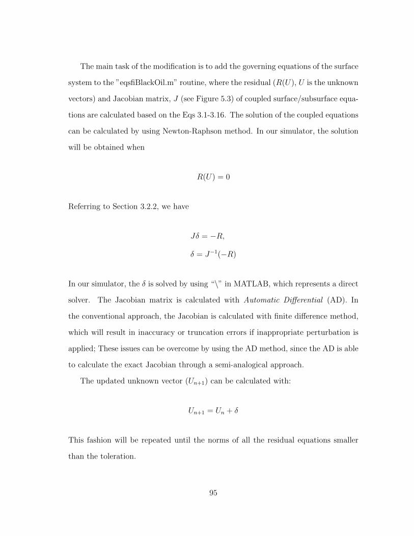
The main task of the modification is to add the governing equations of the surface

system to the ”eqsfiBlackOil.m” routine, where the residual (R(U), U is the unknown

vectors) and Jacobian matrix, J (see Figure 5.3) of coupled surface/subsurface equa-

tions are calculated based on the Eqs 3.1-3.16. The solution of the coupled equations

can be calculated by using Newton-Raphson method. In our simulator, the solution

will be obtained when

R(U) = 0

Referring to Section 3.2.2, we have

Jδ = −R,

δ = J−1(−R)

In our simulator, the δ is solved by using “\” in MATLAB, which represents a direct

solver. The Jacobian matrix is calculated with Automatic Differential (AD). In

the conventional approach, the Jacobian is calculated with finite difference method,

which will result in inaccuracy or truncation errors if inappropriate perturbation is

applied; These issues can be overcome by using the AD method, since the AD is able

to calculate the exact Jacobian through a semi-analogical approach.

The updated unknown vector (Un+1) can be calculated with:

Un+1 = Un + δ

This fashion will be repeated until the norms of all the residual equations smaller

than the toleration.

95

Figure 5.3: Jacobian matrix of fully coupled model

5.2 Validation Test of the Modified MRST Fully Coupled Model

Prior to the investigation with fully implicit model, the validation of the fully

coupled model is tested. This section focuses on checking the consistencies between

the modified MRST and INTERSECT Field Management (IX). Since the injection

network is currently not supported within INTERSECT Field Management, the

injection system is decoupled in the modified MRST fully coupled model for com-

parison. Both commercial and our coupled models are performed under the same

96

reservoir conditions and production strategy. The coupled model used for validation

test is the Scenario-3, which is used in the chapter 4.

The comparison of the production results from modified MRST fully coupled

model and INTERSECT Field Management system is shown Figure 5.4-5.7. The 5-

spot water-flooding pattern is used in study case. Since the PROD-1 has higher pro-

duction rate, the results of PROD-1 is separated from the results of other producers.

The dash lines represent the results obtain from INTERSECT Field Management,

where the coupling frequency (Nc) is set to 15; while the solid lines represent the

results from modified MRST fully implicit coupled model.

Referring to the compared results displayed, the bottom hole pressure profiles

show a difference after the water is produced. This can be explained as that emulsion

effect is considered for oil-water mixture in PIPESIM, which will result in a higher

viscosity when water cut ranges between 30% and 50%. Therefore, the pressure loss

due to the friction is higher when consider emulsion effect.

97

Figure 5.4: Comparison of oil production rates from modified MRST and INTER-

SECT field management

98

Figure 5.5: Comparison of gas-oil ratio from modified MRST and INTERSECT field

management

99

Figure 5.6: Comparison of water production rates from modified MRST and INTER-


100

Figure 5.7: Comparison of bottom hole pressure from modified MRST and INTER-


By observing the Gas-oil ratio (GOR) and BHP profiles, it can be found that

the BHP of producers decreases while GOR is increasing, this is because that the

increasing GOR indicates the existence of free gas within reservoir and tubings, and

the free gas will reduce the average density of the mixture within the tubing, and

consequently reduce pressure loss caused by potential energy. Thus, the decreasing

BHP can be observed when GOR is increasing. When water breakthrough occurred,

the invasion water will again increase the wellbore fluid density,and consequently

101

increase BHP can be observed after water breakthrough.

5.3 The Effect of Coupled Surface Model on Production Performance

This section aims on investigating the impacts of different settings within the

surface network on production performance. The discussion of the impacts can be

used to improve the field management and operation strategies.

In this section, the reservoir model of Scenario-3 will be used. The surface network

model includes one injection well and four production wells. For injection system,

the boundary is located at the wellhead, while the production system is terminated

at separator. The production strategy and properties of the base surface network

model are displayed in Table 5.1.

Table 5.1: Production strategy and properties of the surface network model

Production/injection system settings Value Unit

Production/injection Tubing ID 3 in

production/injection Tubing Length 3005 ft

Production Pipe ID 3 in

Production Pipe Length 1000 ft

Downstream pressure 300 psia

Upstream pressure (at bottom hole) 2700 psia

Roughness 0.001

102

5.3.1 Effects of tubing size

This study will discuss the effect of tubing size on pressure loss and produc-

tion performance. Four cases are performed in this study, different production tub-

ing/pipe sizes are used. The are 1.5”, 2”, 2.5” and 3” respectively. The Injection and

production profiles are displayed in Figure 5.8-5.16, each color represent the result

obtained with each tubing size.

Figure 5.8: Injection profiles for investigating the effects of tubing size

103

Figure 5.9: Oil production rates for investigating the effect of tubing size (PROD-1

and PROD-2)

104

Figure 5.10: Oil production rates for investigating the effect of tubing size (PROD-3

and PROD-4)

105

Figure 5.11: Gas-oil ratio for investigating the effect of tubing size (PROD-1 and

PROD-2)

106

Figure 5.12: Gas-oil ratio for investigating the effect of tubing size (PROD-3 and

PROD-4)

107

Figure 5.13: Water production for investigating the effect of tubing size (PROD-1

and PROD-2)

108

Figure 5.14: Water production for investigating the effect of tubing size (PROD-3

and PROD-4)

109

Figure 5.15: Bottom hole pressure of producers for investigating the effect of tubing

size (PROD-1 and PROD-2)

110

Figure 5.16: Bottom hole pressure of producers for investigating the effect of tubing

size (PROD-3 and PROD-4)

111

Referring to Figure 5.7 and Figure 5.11, it can be observed that all producers

with a smaller tubing size have a higher BHP profiles. Thus, it can be concluded

that the tubing with smaller diameter has more restriction (due to friction) to the

fluid flow, and consequently result in a larger pressure loss through the tubing. By

observing oil production profiles, it is found that the oil production rate is relative

high when using larger tubing size, this is due to the lower BHP of producers and

higher water injection. From Figure 5.11-5.12, it can seen that the case of large

tubing size will lead to more free gas existing within the reservoir, which indicates

that the reservoir pressures drop faster. This can be explained as that when using

large tubing, the oil production rate is too high and the water injection rate is hard

to maintain energy within the formation, therefore we can observe more free gas

produced from production wells. From the discussion above, it can be conclude

that using large production tubing could result a high oil production rates at the

beginning. However, oil production will drop rapidly and the reservoir energy is

hard to be maintained by using large tubing producers, thus it is recommended to

use relative small tubing size for production, in order to maintain the energy within

the reservoir.

5.3.2 Effects of adding a choke

At the early time of oil production, the production rate is very high without

restriction. Generally, it is necessary to restrict the flow rate in order to prevent sand

production and gas coning in the oil reservoir. However, using a high downstream

pressure (i.e. separator pressure) to restrict production rate is not applicable in

the field. Therefore, the choke is required for restricting production rate as well as

keeping the downstream pressure at standard conditions.

In order to study the effect of choke on production performance, we need to

112

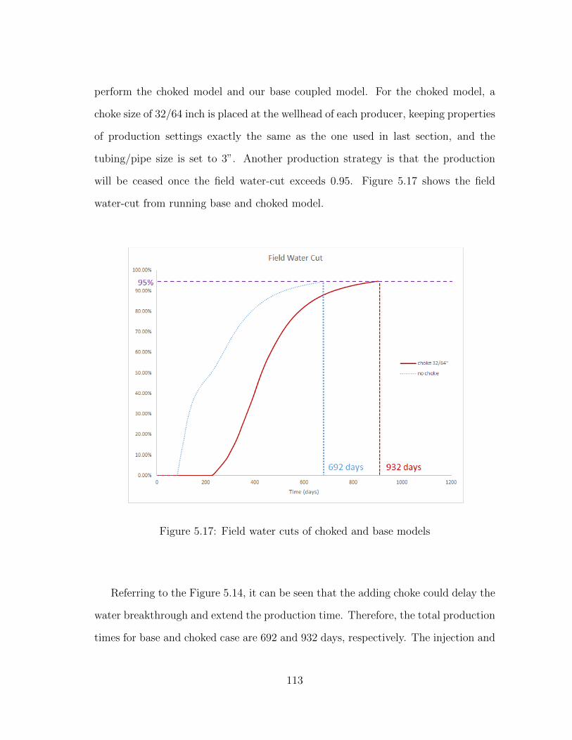
perform the choked model and our base coupled model. For the choked model, a

choke size of 32/64 inch is placed at the wellhead of each producer, keeping properties

of production settings exactly the same as the one used in last section, and the

tubing/pipe size is set to 3”. Another production strategy is that the production

will be ceased once the field water-cut exceeds 0.95. Figure 5.17 shows the field

water-cut from running base and choked model.

Figure 5.17: Field water cuts of choked and base models

Referring to the Figure 5.14, it can be seen that the adding choke could delay the

water breakthrough and extend the production time. Therefore, the total production

times for base and choked case are 692 and 932 days, respectively. The injection and

113

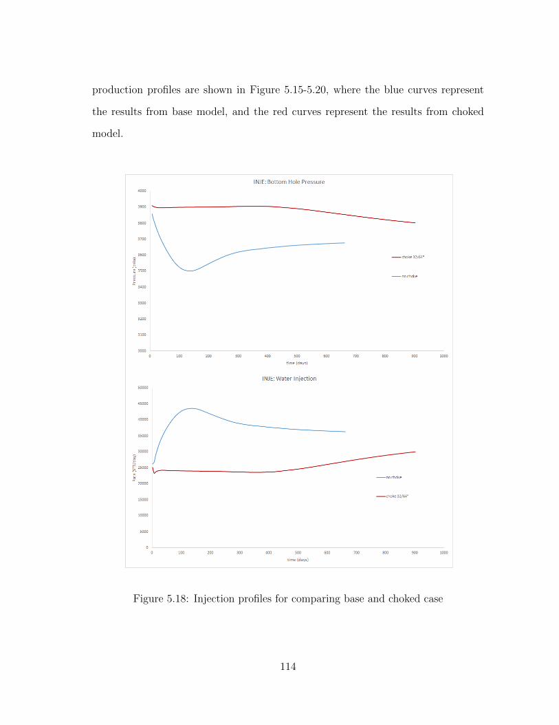
production profiles are shown in Figure 5.15-5.20, where the blue curves represent

the results from base model, and the red curves represent the results from choked

model.

Figure 5.18: Injection profiles for comparing base and choked case

114

Figure 5.19: Oil production for comparing base and choked case (PROD-1 and

PROD-2)

115

Figure 5.20: Oil production for comparing base and choked case (PROD-3 and

PROD-4)

116

Figure 5.21: Gas liquid ratio for comparing base and choke case (PROD-1 and

PROD-2)

117

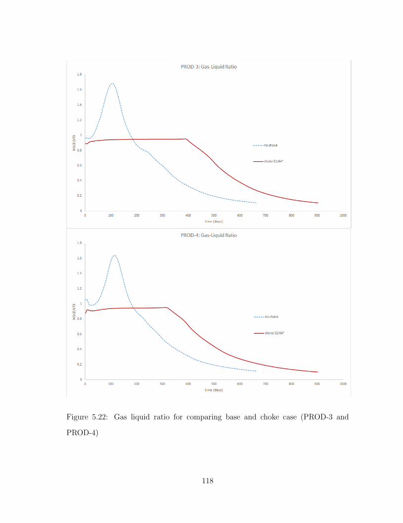
Figure 5.22: Gas liquid ratio for comparing base and choke case (PROD-3 and

PROD-4)

118

Figure 5.23: Bottom hole pressure for comparing base and choke case (PROD-1 and

PROD-2)

119

Figure 5.24: Bottom hole pressure for comparing base and choke case (PROD-3 and

PROD-4)

120

Figure 5.25: Reservoir pressure for comparing base and choke case

Figure 5.26: Cumulative oil production for comparing base and choked case

121

By observing injection profiles, a higher BHP and lower injection rate can be

found in the choked case, this indicates a high reservoir pressure around the injection

well. From the oil production profile, it can be seen that the oil production rate

is restricted by the choke within the desired range; also the time for constant oil

production is extended due the placed choke. Although the cumulative production

of the choked case increases slower than that of base case, the final oil recovery is

increased by 198885 STB in the choked case, due to the longer production time.

Referring to the Figure 5.18 and 5.19, it is found that the producers’ BHPs start

to decline after water breakthrough, this can be explained as that the Gas-Liquid

Ratio (GLR) will be reduced when well starts to produce water, and smaller GLR

will results in a smaller upstream pressure at choke, consequently results in a lower

BHP. Therefore, the decline in producers’ BHP can be observed when water enter

the production tubing.

5.4 Performing Fully Coupled Simulator with Realistic Scenario

In this section, we tested the stability of our in-house simulator to more realistic

scenario. The coupled and non-coupled model will be compared, in order to inves-

tigate the effect of surface network elements on the production performance. The

reservoir model that used in this study is the SPE-10 benchmark25.

5.4.1 Description of reservoir model and properties of fluid

In general, our simulator is able to apply the couplings to a black-oil 3D model.

However, since there are over one million grid blocks within the SPE-10 benchmark,

we only modeled the first layer of SPE-10 in this study, in order to save on the

computational cost. The description of SEP-10 reservoir model is summarized in

Table 5.2.

122

Table 5.2: Descriptions of SPE-10 reservoir model

Reservoir Conditions Value Unit

Nx : Ny : Nz 60:220:1 ft

∆x×∆y ×∆z 6×3×2

permeability Heterogeneous (refer to Fig 5.21) mD

Porosity Heterogeneous (refer to Fig 5.21) %

Reservoir Initial Pressure 6000 Psia

Initial Water Saturation 0 %

Initial Oil Saturation 100 %

Reservoir Top Depth 12000 ft

Production Scenario 5-spot water flooding

Both the permeability and porosity of SPE-10 reservoir model are heterogeneous,

and the permeability ranges from 0 to 4650 mD, while the porosity is between 0 and

0.45, Their maps are shown in Figure 5.27.

123

Figure 5.27: Permeability and porosity map of SPE-10 benchmark

124

Referring to Figure 5.27, it can be seen that the production scenario is a 5-spot

water flooding pattern, where the injection well is placed at the center of reservoir

that has low porosity and permeability.The four producers are placed at four cor-

ners of the reservoir respectively; the PROD-3 and PROD-4 are located at the high

permeability zones.

5.4.2 Production strategy and facilities’ properties

The production strategy and facility properties of coupled case is shown in Table

5.3. For the non-coupled case, only the production strategy is shown in Table 5.4.

Table 5.3: Production strategy and facility properties used for coupled case

Production strategy & facility properties Value Unit

Production Tubing ID 2 in

production Tubing Length 12000 ft

Surface Pipe ID 2 in

Surface Pipe Length 1000 ft

Downstream production pressure 200 psia

Upstream injection pressure 2000 psia

Roughness 0.001

Choke size 3/64 inch

125

Table 5.4: Production strategy used for non-coupled case

Production strategy Value Unit

Downstream production pressure 3650 psia

Upstream injection pressure 7460 psia

5.4.3 Results and discussions

The results of comparing coupled and non-coupled cases are shown in Figure

5.28-5.32, where the red curves represent the results from performing coupled model,

while the blue curves represent the results from non-coupled case. Since the difference

between coupled and non-coupled case is not obvious for PROD-1, PROD-2 and

PROD-4, only the production profiles of PROD-3 are shown.

Figure 5.28: Oil production for comparing coupled and non-coupled with SPE-10

case

126

Figure 5.29: Water production for comparing coupled and non-coupled SPE-10 case

Figure 5.30: Bottom hole pressure for comparing coupled and non-coupled SPE-10

case

127

Figure 5.31: Gas-liquid ratio for comparing coupled and non-coupled SPE-10 case

Figure 5.32: Total cumulative oil production

128

By observing the water production profile, we find that the water breakthrough

only occurred in PROD-3. Since the gas-oil ratio kept constant during the pro-

duction, it is inferred that there is no free gas entered the production tubing, and

therefore, the bottom hole pressure kept is constant before the breakthrough. For

PROD-3, an increase of bottom hole pressure can be observed after water break-

through, this is differs from what concluded in last chapter that the decreased GLR

will reduce the bottom hole pressure for choked model, this implies that the bottom

hole pressure is affected by both the GLR and mixture density in the tubing, when

the flow rate is small, the change of pressure caused by change of GLR will be small,

therefore, the mixture density will be the dominating factor that impacts the bottom

hole pressure of producers.

By comparing the coupled and non-coupled cases, it is found that the non-coupled

failed to predict the bottom behavior after water breakthrough, which will results in

overestimation of water production and oil recovery.

The total iterations of running coupled and non-coupled cases are summarized in

Table 5.5. It is found that fully coupling will increase both the iterations and sim-

ulation time. Referring to the Newton-Raphson, we counted the Newton iterations

for all the timesteps. The iterations of each timestep for the two cases are shown

in Figure 5.33. It can be seen that the coupled model used more Newton iterations

at the beginning of production. Also, it is concluded that the CPU time of coupled

model is 2.95 times of the non-coupled case. However, the difference in total recov-

ery from coupled and non-coupled cases are not obvious. Therefore, in order to save

computation time, it is recommended to use non-coupled model when perform the

SPE-10 scenario.

129

Table 5.5: Summary of iterations and elapsed time

model type iterations Elapsed time (s)

coupled 718 1621.79

non-coupled 671 510.5

Figure 5.33: Iterations of each timestep for comparing the coupled and non-coupled

model

130

6. CONCLUSIONS AND RECOMMENDATION

6.1 Summary and Conclusions

We have investigated the fluid flow characteristics within the porous media and

the surface network; and studied the mechanism of different coupling approaches.

Four scenario were constructed and through a sensitivity study we assessed the im-

pact of coupling frequency on production performance under different scenario.

The construction of a fully coupled model that includes both the production

system and injection system realized the production prediction considering the entire

surface facilities. In addition, the flexible code implementation allows incorporation

of additional physics in the simulator. With the in-house fully coupled model, we

have investigated the effect of network settings on production performance.

Based on the completed tasks, we conclude:

• For the partially implicit coupling, the coupling frequency has impact on the

simulation efficiency and production performance. It is found that using low

coupling frequency could reduce the computational time. However, low cou-

pling frequency may fail to accurately predict the production, since the in-

complete balance action cannot predict the state of bottom at the end of each

timestep;

• The high permeability reservoir shows more sensitivity to coupling frequency

than low permeability reservoir in terms oil and gas recovery;

• The oil/gas production forecast of heterogeneous permeability reservoir is more

sensitive to coupling frequency than that of homogeneous permeability reser-

voir;

131

• When partially coupling performed under unconventional reservoir, the im-

pacts of coupling frequency on simulation results is insignificant, because the

production states keep constant during the production, and a complete balance

of reservoir/network can be achieved by using low coupling frequency.

• At early time of production, the gas-oil ratio is the dominating factor that

impacts the bottom hole pressure of producers. It is found that the increased

gas-oil ratio will reduce the bottom hole pressure of producers. When the water

breakthrough occurred, the bottom hole pressure is mainly dependent on the

fraction of water within the tubing; it is found that the pressure will increase

with the increasing water production rate;

• The production tubing size has impact on well boundary conditions, it is found

that for producers, the small tubing size will restrict the flow rate, and increase

the flowing pressure at bottom hole.

• For the model with choke restricted, the bottom hole pressures of producers

are mainly determined by both the gas-liquid ratio and mixture density within

the tubing. When flow rate is high, the GLR will be the dominating factor

that determines the bottom hole pressure of producers;

• By placing the choke at the wellhead, the oil production rate can be constrained

within the desired pressure limit; also the improve the voidage replacement;

• By performing different experiments with several coupling methods, includ-

ing partially coupled, fully coupled and non-coupled model, we concluded that

the selection of coupling method depends on the particular reservoir. When

performing the simulations under unconventional reservoir (e.g. tight-oil reser-

voir), where the variation of production behavior and well boundary condition

132

in time is insignificant, the non-coupled simulator is recommended in order to

save computation time. When the simulation is performed under conventional

reservoir, where significant variations of production states and well bound-

ary conditions in time may occur, then the fully coupling and high coupling

frequency partially coupling is recommended. The advantages of partially cou-

pling is that by well tuned coupling frequencies, one can couple two individuals

external commercial software with great computational saving. However, when

using partially coupling method, one has to be careful with oscillations into the

solution, therefore, the fully coupling method is recommended with the con-

siderations of stable solutions and fast convergence.

6.2 Future Work

Based on our research studies, a suggestions will be given regarding the future

work of this project.

In real production field, the production operation strategy is more complicated.

In our research, only one water flood pattern is considered. However, in the real-

istic scenario, the production field could consist of multiple unit of water flooding

pattern. Another assumption made in our project is that all the production wells

is simplified vertical wellbore model, thus the coupled model can further consider

more complicated wellbore models, such as horizontal or multilayers wellbore model.

The research study can be further developed by considering the transient flow within

each timestep. As mentioned in chapter 2, we assumed that the tubing/pipe flow

is in steady state, which could result in inaccuracy of the pressure loss calculation.

Thus, it is necessary to consider the transient flow in the more complicated models.

By implementing these suggestions into the future studies, a more comprehensive

conclusion of surface/subsurface coupling would be achieved.

133

REFERENCES

1. Holmes, J.A.: “Enhancements to the Strongly Coupled, Fully Implicit Well

Model: Wellbore Crossflow Modeling and Collective Well Control,” paper SPE

00012259 presented at the 1983 SPE Reservoir Simulation Symposium.

2. Holmes, J.A., Barkve, T. and Lund, O.: “Application of a Multisegment Well

Model to Simulate Flow in Advanced Wells,” paper SPE 50646 presented at

the 1988 SPE European Petroleum Conference. Hague, 20-22 October.

3. Stone, T.W. et al.: “Thermal Simulation with Multisegment Wells,” paper SPE

66373 presented at the 2001 SPE Reservoir Simulation Symposium, Houston,

11-14 February.

4. Dempsey, J.R. et al.: “An Efficient Method for Evaluating Gas Field Gathering

System Design,” JPT (September 1971) 1067.

5. Beggs, H.D.: “An Experimental Study of Two-Phase Flow in Inclined Pipes,”

PhD dissertation, U. of Tulsa (1972).

6. Startzman, R.A. et al.: “Computer Cobines Offshore Facilities and Reservoir

Forecast,” Petroleum Engineer (May 1977) 65.

7. Feng, W.Y. and Lom K.K.: “A Generalized Well Management Scheme for

Reservoir Simulation,” SPE Reservoir Engineering (May 1996) 116-120.

8. Wijestinghe, A.M.: “A Comprehensive Well Management Program for Black

Oil Reservoir Simulation,” paper SPE 12260 presented at the 1983 SPE Sym-

posium on Reservoir Simulation, San Francisco, Nov. 15-18.

134

9. Schiozer, D.J. and Aziz, K.: “Use of Domain Decomposition for Simultaneous

Simulation of Reservoir and Surface Facilities,” paper SPE 27876 presented at

the 1994 SPE Western Regional Meeting, Long Beach, California, 23-25 March.

10. Byer, T.J., Edwards, M.G. and Aziz, K.: “Preconditioned Newton Methods

for Fully Coupled Reservoir and Surface Facility Models,” paper SPE 49001

presented at the 1988 SPE Annual Technical Conference and Exhibition, New

Orleans, 27-30 September.

11. Coats, B.K., Fleming, G.C., Watts J.W., Rame, M. and Shiralkar, G.S.: “A

Generalized Wellbore and Surface Facility Model, Fully Coupled to a Reservoir

Simulator,” Reservoir Evaluation and Engineering (April 2004) 132.

12. Guyaguler, B. et al.: “Near-Well Subdomain Simulations for Accurate In-

flow Performance Relationship Calculation to Improve Stability of Reservoir-

Network Coupling,” paper SPE 141207 presented at 2011 SPE Reservoir Sim-

ulation Symposium, Woodlands, 21-23 February.

13. Hayder, E.M., Dahan, M. and Dossary, M.N.: “Production Optimization through

Coupled Facility/Reservoir Simulation,” paper SPE 100027 presented at the

2006 Intelligent Energy Conference and Exhibition.

14. Ursini, F., Rossi, R. and Pagliari, F.: “Forecasting Reservoir Management

through Integrated Asset Modeling,” paper SPE 128165 presented at the 2010

North Africa Technical Conference and Exhibition.

15. Gonzalez, F.E. et al.: “A Fully Compositional Integrated Asset Model for a

Gas-Condensate Field,” paper SPE 134141 presented at the 2010 SPE Annual

Technical Conference and Exhibition.

135

16. Ghorayeb, K. et al.: “A General Purpose Controller for Coupling Multiple

Reservoir Simulations and Surface Facility Networks,” paper SPE 79702 pre-

sented at the 2003 SPE Reservoir Simulation Symposium, Houston, Texas,

USA (February 3-5, 2003).

17. Hepguler, G., Barua, S. and Bard, W.: “Integration of Field Surface and Pro-

duction Network with a Reservoir Simulator,” SPECA (June 1997) 88.

18. Guyaguler, B. and Ghorayeb, K.: “Integrated Optimization of Field Develop-

ment, Planning, and Operation,” paper SPE 102557 presented at 2006 SPE

Annual Technical Conference and Exhibition, San Antonio, 24-27 September.

19. INTERSECT Version 2013.1 Reference Manual, Schlumberger Information

Systems.

20. Ertekin, T., Abou-Kassem, J.H., King, G.R., Basic Applied Reservoir Simula-

tion (1993), Richardson, Texas: Textbook Series, SPE

21. Economides, M.J., Hill, A.D., Ehlig-Economides, C. and Zhu, D., Petroleum

Production Systems (January 2013), Upper Saddle River: Prentice Hall.

22. Hagedorn, A.R. and Brown, K.E.: “Experimental Study of Pressure Gradi-

ants Occurring During Continuous Two-Phase Flow in Small-Diameter Vertical

Conduits,” J. Pet. Tech. (April 1965) 475-484.

23. PIPESIM Version 2013.1 User’s Guide, Schlumberger Information Systems.

24. Trick, M.D.: “A Different Approach to Coupling a Reservoir Simulator with a

Surface Facility Model,” paper SPE 00040001 presented at the 1998 SPE Gas

Technology Symposium.

136

25. Christie, M. and Blunt, M.: “SPE Comparative Solution Project,” retrieved

July 15, 2014, from http://www.spe.org/web/csp//

26. Lie, K.-A., Krogstad, S., Ligaarden, I. S., Natvig, J. R., Nilsen, H. M., and

Skaflestad, B.: “Open source MATLAB implementation of consistent discreti-

sations on complex grids,” retrieved August 10, 2014, from http://www.sintef.c-

om/Projectweb/MRST/

137

RESERVOIR AND SURFACE FACILITIES COUPLED THROUGH PARTIALLY...

Documents

Transcript of RESERVOIR AND SURFACE FACILITIES COUPLED THROUGH PARTIALLY...