RESERVE PRICE DETERMINANTS IN PROZORRO AUCTIONS IN … · ProZorro auctions. The main objective of...

RESERVE PRICE DETERMINANTS IN PROZORRO AUCTIONS IN

UKRAINE

by

Anton Liutov

A thesis submitted in partial fulfillment of the requirements for the degree of

MA in Economic Analysis .

Kyiv School of Economics

2018

Thesis Supervisor: Professor Pavlo Prokopovych Approved by ___________________________________________________ Head of the KSE Defense Committee, Professor Tymofiy Mylovanov

__________________________________________________

__________________________________________________

__________________________________________________

Date ___________________________________

Kyiv School f Economics

Abstract

RESERVE PRICE DETERMINANTS IN PROZORRO AUCTIONS IN

UKRAINE

by Anton Liutov

Thesis Supervisor: Professor Pavlo Prokopovych

This paper examines allocations between reserve prices and winning bids in

ProZorro auctions. The main objective of this study is to show how a one

percent change in reserve price affects winning bids and vice versa, how a one

percent change in winning bid affects reserve prices. We also introduce a number

of variables which explain the observed fluctuations of reserve prices and winning

bids.

TABLE OF CONTENTS

CHAPTER 1. INTRODUCTION ...............................................................................1

CHAPTER 2. LITERATURE REVIEW ....................................................................4

2.1. Theoretical studies ...............................................................................................4

2.2. Empirical studies ..................................................................................................7

CHAPTER 3. METHODOLOGY ..............................................................................11

3.1. Final price determinants .....................................................................................11

3.2. Reserve price determinants ................................................................................14

CHAPTER 4. DATA DESCRIPTION.......................................................................15

CHAPTER 5. EMPIRICAL RESULTS ......................................................................23

3.1. Final price determinants for gasoline, eggs and potato .................................23

3.2. Reserve price determinants for gasoline, eggs and potato ...........................27

CHAPTER 6. CONCLUSIONS ...................................................................................30

WORKS CITED ..............................................................................................................32

APPENDIX A. CHECKING FOR MULTICOLLINEARITY ...........................34

APPENDIX B. BREUSCH-PAGAN TESTS ...........................................................38

APPENDIX C. EMPIRICAL RESULTS FOR THE MODEL (2) FOR EGGS AND POTATO ................................................................................................................39

APPENDIX D. EMPIRICAL RESULTS FOR THE MODEL (4) FOR EGGS AND POTATO ................................................................................................................41

ii

LIST OF FIGURES

Number Page

Figure 1. The reserve price for eggs and potato for the period of 2016-2018 ......16

Figure 2. The winning bid for eggs and potato for the period of 2016-2018 ........18

Figure 3. The reserve price and the final price for gasoline for the period of 2016-2018 ......................................................................................................................................19

Figure 4. Location of buyers over the country ............................................................20

Figure 5. Number of bidders and macroeconomic variables ....................................22

Figure 6. Correlation between independent variables for the model (2) for gasoline ................................................................................................................................34

Figure 7. Correlation between independent variables for the model (2) for eggs .35

Figure 8. Correlation between independent variables for the model (2) for potato ..............................................................................................................................................35

Figure 9. Correlation between independent variables for the model (4) for gasoline ................................................................................................................................36

Figure 10. Correlation between independent variables for the model (4) for eggs ..............................................................................................................................................36

Figure 11. Correlation between independent variables for the model (4) for potato ...................................................................................................................................37

iii

LIST OF TABLES

Number Page

Table 1. Summary statistics of the reserve price ...................................................... 16

Table 2. Summary statistics of the winning bid ........................................................ 17

Table 3. Number of bidders and macroeconomic variables .................................. 20

Table 4. Final price determinants of gasoline ........................................................... 24

Table 5. Reserve price determinants of gasoline ...................................................... 28

Table 6. Breusch-Pagan tests for models (2) and (4) ............................................... 38

Table 7. Final price determinants of eggs .................................................................. 39

Table 8. Final price determinants of potato .............................................................. 40

Table 9. Reserve price determinants of eggs ............................................................. 41

Table 10. Final price determinants of eggs ................................................................ 42

iv

ACKNOWLEDGMENTS

The author wishes to express his gratitude to his thesis advisor, Professor Pavlo

Prokopovych, for helping with doing the research, correcting mistakes, constant

support whenever the author requires it, finding the proper way of solving issues

occur with the thesis, any helpful suggestions.

The author is willing to thank all the professors who participated in the Research

Workshops, where they gave invaluable advices and corrected mistakes. In

addition, a special gratitude to Natalia Kalinina for helping to edit his thesis with

using proper English.

v

GLOSSARY

PBE – Perfect Bayesian Equilibrium

MPE – Markov Perfect Equilibrium.

GDP – Gross Domestic Product.

CPI – Consumer Price Index.

INDOT – Indiana Department of Transportation.

OLS – Ordinary Least Squares.

C h a p t e r 1

INTRODUCTION

An auction is a widespread resource for people who want to buy or sell an object

with maximum payoff by collecting bids from participants. There are different

forms of auctions and their primary objectives. The best-analyzed and well-

known auctions are the English auction, the Dutch auction, the first-price sealed-

bid auction and the second-price sealed-bid auction for selling single object in the

first round. All of them are quite important in terms of profit optimization of

organizers as well as participants of auctions. It is worth mentioning that all the

auctions listed so far are static. However, what can be said about dynamic

auctions with two rounds or even more. There is, for instance, the procurement

auction organized by the Indiana Department of Transportation (INDOT),

which has several rounds where bidders propose their own bids in the first round

and then after observing a new information make the second offer for organizers.

This auction is of interest because such an auction could increase payoff for

organizers as well as for participants. There are studies about such auctions. Lu Ji

(2006) studies multi-round procurement auctions with reserve prices and with

forward-looking bidders. He uses different statistical tools. For example, Perfect

Bayesian Equilibrium and Markov Perfect Equilibrium in order to find the

optimal set of strategies for bidders. Elyakime et al. (1997) study the auction with

two rounds, where the first round is the same as for the first-price sealed bid

auction. If the object is left unsold then the second round is conducted where the

seller and the bidder with the highest bid in the previous round bargains about

the optimal price of the object. In the next section, we consider literature in more

detail in order to familiarize us with works done so far. Those papers are taken as

2

a basis for this study and can be taken for subsequent researches in the auction

theory.

Our study focuses on public procurement auctions in Ukraine for ProZorro

system launched in 2015. This system is intended to reduce corruption in

auctions and can help to save money for government. The data consist of 1970

auctions for the period of 2016-2018. Actually, this is a very small sample of data

available on the website of the e-procurement system. In this auction, the buyer is

the organizer of the auction and bidders are sellers. Thus, the buyer tries to

minimize his own costs for purchasing objects. In order to do this he can set the

initial reserve price that could decrease or increase the price for which he will buy

objects. There are different factors that can affect the reserve price and the price

for which sellers are ready to sell objects. In this study, we focus in detail on these

parameters. It is assumed that characteristics of the auction could have an impact

on the reserve price and the winning bid and such relation was investigated in a

lot of papers. That is why, this paper introduces new variables, which can have

effect. For example, changes in GDP, inflation, interest rate set by the National

Bank of Ukraine, in exchange rate for USD, the reserve price and the winning bid

in the previous period that is the previous month and dummy for quarters.

Macroeconomic variables are assumed to be important for estimating decisions

of participants of auctions.

The first contribution of this paper is to show the allocation between

independent variables and dependent variables, which are the reserve price and

the winning bid in case of Ukraine. The second contribution is to explore new

determinants of variation in the reserve prices and the winning bids. As a result,

both the buyers and the sellers get additional information about how to decrease

their own costs and which factors are the most important. So this study is

intended to enforce the ability of players of auctions to be more rational in terms

3

of optimization their strategies as they may be confused about how to set bids in

the most correct way. Whether they should base their decision on the previous

experience or not.

The data are collected from ProZorro auctions and have 1970 auctions with

below threshold procedures. All auctions are conducted within the period of

2016-2018 years. Besides that, it is examined for all regions of Ukraine

participated in auctions for the given period of time. Gasoline, potato and eggs

are used as products for modelling the relation between the reserve price and the

winning bid. Macroeconomic variables are collected from www.ceicdata.com.

The first finding of this paper is confirming of a positive correlation between the

reserve price in the current period and the winning bid in the previous period. So

an increase by 1% in the final price causes an increase in the reserve price by 0.1-

0.5% depending on the product type. The second finding is confirming a positive

correlation between the winning bid and the reserve price in the current period.

So an increase by 1% in the reserve price causes an increase in the winning bid by

0.5-0.7%. In addition, the unique number of bidders is influential variable and

macroeconomic variables are important in describing participants’ behavior of

auctions depending on the product type.

The reminder of the article is constructed as follows. In the subsequent Chapter,

we review theoretical and empirical literature on static and dynamic auctions. In

Chapter 3, we construct the methodology for analyzing allocation between the

reserve price and the winning bid based on previous studies. Data description is

shown in Chapter 4. Chapter 5 shows the results of models for available statistical

data across regions, three types of products (gasoline, potato and eggs) for below

threshold procedures by using OLS regressions. Conclusions and

recommendations for further studies are provided in Chapter 6.

4

C h a p t e r 2

LITERATURE REVIEW

An intense interest in e-procurement auctions has rapidly grown over the last

years. Many of scientists in the field of the auction theory investigate patterns of

bidders’ behavior in auctions in order to find an efficient design of an auction or

maximize payoffs for organizers or bidders. Thus, it is well-known that a lot of

papers on this topic have been emerged so far. It is worth noting that scientists

work with different designs of auctions. One of very widespread auctions is the

eBay auction. It is close to the second-price sealed bid auction, but with some

modifications. The seller sets a duration of the auction with a minimum starting

bid or reserve price. After the auction starts, bidders make their offers for the

seller by bidding. It is worth mentioning that participants can adjust their

valuation and bid multiple times. Eventually, the bidder with the highest bid will

buy the object for the second highest bid with small increment.

2.1. Theoretical studies

Roth and Ockenfles (2000) study how last-minute bidding and the rules for

ending the second-price auctions could change bidders’ behavior. They find that

the difference in rules of duration of eBay and Amazon auctions have an

important element for the auction design. Bids of participants during the auction

for eBay and Amazon differ substantially, but converge to the same bid at the end

of the auction. There are a lot of studies about the second-price sealed bid

auction (e.g. Lo 1998, Isaac et al. 2007).

5

For example, Lo (1998) studies sealed bid auctions with uncertainty and averse

bidders. He finds that the first-price sealed bid auction Pareto dominates the

second-price sealed bid auction. In addition, the author concludes that risk averse

participants of auctions strictly prefer the first-price auction rather than the

second-price auction. Isaac et al. (2007) investigate bidder’s behavior in the

second-price auction with the unknown number of bidders. He finds a strong

support for the fact that bidders in their strategies are close to the dominant

strategy in the second-price auction with the known number of bidders. There are

other papers, but they are not of our interest. Thus, let us focus on multi-round

auctions.

Multi-round auctions play an essential part in the auction theory. The design of

such auctions allow bidders to adjust their bids in time and compete with each

other more aggressively. As a result, an organizer of such actions increases his

payoff. There are studies that investigate how bidders should behave in order to

get the most from the auction. Lu Ji (2006) studies multi-round auctions with the

reserve price and forward-looking bidders. He considers the auction where

bidders try to make a contract with government. The organizer sets the reserve

price, which is the minimum amount for which the organizer is ready to buy the

object. The bidder with the lowest bid wins the first round, but if that bid is

higher than the reserve price then the second round is launched. Thus, there is a

positive probability that the object will remain unsold that causes inefficiency. As

a result of this study, the author finds that the reserve price is an important part

of an auction and can raise the revenue for government.

Jofre-Bonet and Pesendorfer (2003) study a repeated auction game, where they

consider bids of participants, contracts’ characteristics and bidders’ state for

making their model for estimating the optimal set of bidders’ strategies. As a

result, they evaluate empirically the repeated highway construction procurement

6

auctions in the state of California for the period from May 1995 till May 1999 by

using Markov Perfect Equilibrium (MPE). As a result of their study, they

conclude that timing of contracts has some impact on the final price of the object

and there may be present some inefficiency in choosing firms as the winner. Reiß

et al. (2008) show bidders’ behavior in the first-price auction in a sequential game

with two rounds and with capacity constraints for firms. They construct the game

with two risk-neutral firms and two projects, which are sequentially auctioned off.

The authors use a Perfect Bayesian Equilibrium (PBE) for finding the optimal

result. Thus, they find that in a sequential game, firms may not participate in the

first round, but all of firms take part in the second stage. As a result of the

investigation, the authors find that firms that win the first round reduce the

probability to win in the second round as such firms increase their cost to buy

additional product. So firms adjust their own behavior according to the future

costs.

There is one more interesting article about dynamic games written by Bajari et al.

(2007). This article estimates a dynamic game with N firms, which take into

account the future value function as their future opportunity for winning another

object. That’s why, authors introduce a Markov Perfect Equilibrium. The main

objective of this study is to obtain information about bidders’ beliefs. As a result,

authors find that their Monte Carlo approach is computationally easier than for

static models and can be applied for revealing agent’s beliefs.

Also, there is quite an interesting article written by Paarsch et al. (2002). Authors

determine a strategic equilibrium of the multi-unit, sequential, ascending price

auctions. By analyzing such game, they find out how to get the efficient allocation

and equilibrium algorithm for revealing the winning price for the object. They

conclude that if a bidder is willing to buy only one unit, the winning prices for a

7

sequence of auctions are the same, but if a bidder is willing to buy more than one

unit, the winning prices will increase over the auction.

2.2. Empirical studies

There are a lot of empirical studies, which estimate how reserve prices and

winning bids are determined by other factors. For example, Choi et al. (2010)

present the estimation of the reserve price impact on auctions outcome from

260,000 online auctions of second-hand cars. Authors try to answer the following

questions: whether variable ‘player entry into auctions’ is not exogenous and what

is the essence of bidders’ valuations. As a result of this study, they conclude that

if the reserve price goes up then the number of bidders decreases, more

experienced bidders remain and they are not sensitive to changes in the reserve

price, the likelihood of the subject to be sold decreases, the expected revenue

increases. Therefore, ‘player entry into auctions’ is endogenous and bidders have

quite a different valuation of the same object.

Wan and Teo (2001) study the factors which influence prices of Internet auctions.

They consider eBay auctions for two coins and potential factors, which can have

some effect on prices. They examine whether the duration of auctions, closing of

auctions on weekend, feedback of sellers, the number of participants have a

positive effect on prices and the minimum bid negatively correlates with auction

prices of objects. As a result of regression analysis, they conclude that the auction

price is positively affected by the number of participants and the minimum bid.

The second and the third findings are the following: the duration of auctions and

feedback of sellers are weakly significant, and the dummy for closing auctions on

weekend is not significant at all.

8

Bajari and Hortacsu (2003) examine bidders’ and sellers’ behavior in eBay

auctions. They use different potential factors affecting prices and try to estimate

changes in prices by using structural econometric model. Based on this model,

they examine winner’s curse and changes in seller profit for different reserve

prices. So after the analysis they can say that bidders try to submit the final bid

close to the end of the auction, sellers try to set their reserve prices approximately

as a minimum bid, which is less than the price of the object and there is a large

variety of the number of participants over auctions. Moreover, they find that one

additional bidder decreases bids by 3.2%, entry plays an important part for sellers’

revenue and sellers, who set the reserve price with a low minimum bid can get

more revenue than sellers who set it higher.

Roberts (2009) tests how endogeneity in auctions can effect on the distribution of

bidders’ values. The author suggests using reserve prices for auctions and a

general nonparametric solution to the problem of identifying bidder’s values.

Thus, he summarizes that the reserve price can help to control for endogeneity

that can cause overestimation of bidders’ distributions of valuation of the object.

Moreover, endogeneity issue can decrease the sellers’ revenue.

Amidu and Agboola (2009) examine determinants of auction premium for the

data for Federal Government Landed Properties in Nigeria. A lot of variables

were used as independent variables. They are the following: property type,

location, number of bedrooms, the size of the plot area, the highest bid, number

of bidders. They prove the theory based on the empirical research that bid prices

are less than zero-profit asset in the first-price sealed bid auction. Also, one of the

main findings is that location and the number of bidders are important

determinants for an auction premium. One more interesting finding of this study

is that corporates tend to submit higher bids.

9

Lucking-Reiley et al. (2007) write the following interesting paper. In the study,

authors investigate determinants of prices in online auctions at the eBay website.

They use the data from July till August 1999 that include over 20 000 auctions.

Their major tool is a descriptive analysis and a regression, which help them to

find the most influential factors in auctions. As a result, they conclude a seller’s

feedback has a large impact on final prices. It is worth noting that a negative

feedback is much stronger than a negative one. In addition, the reserve price and

the final prices have some positive correlation.

Seckin and Atukeren (2011) study Art Auction for the 2005-2008 period. They

study the efficiency of art auctions in Turkey with 11 212 auction records.

Particularly, how unsold paintings could have an effect on estimating the final

price. This study incorporates macroeconomic developments and expectations.

So the main idea of authors is to show that coefficients in regressions are not

biased. After investigation, they conclude that it is true. So unsold paintings

should not be added to the data for the analysis and estimation of relations of

variables. There is quite an extraordinary topic of auctions investigation.

Malisuwan et al. (2015) write “Spectrum Auction Theory and Spectrum Price

Model”. They study how the spectrum auction determines the spectrum price and

whether the spectrum is efficiently assigned. Therefore, the radio spectrum is the

invaluable resource in telecommunications. As a result of investigation, authors

find that the spectrum valuation is an highly influential factor for estimating a

reserve price.

A lot of papers are listed so far. So, the question arises what is the contribution of

this study. Firstly, it uses methodology based on models developed by specialists

in the auction theory and adds new variables in order to extend the literature with

new models. This could improve the accuracy of models. These models

incorporate the reserve price, the winning bid, the dummy for quarter, the

10

number of bidders and macro variables (GDP year over year growth rate, CPI

year over year growth rate and exchange rate of USD). As a result, these new

factors are influential for some products. Gasoline, potato and eggs are used as

products for modelling the relation between the reserve price and the winning

bid. Only three of products are used as there is an issue with collecting unit

prices. Thus, due to the manual collection of data, it is decided to build new

models only for listed goods, but it can be extended to others. In addition, all

regions of Ukraine are included in all models. Secondly, this study contributes to

the literature by exploring the effect of changes in the reserve price by 1% on the

final price in the current period and the effect of change in the final price in the

current period by 1% on the reserve price in the subsequent period. The next

section introduces a base model for the analysis and a new extended version of

this model for two endogenous variables, which are the winning bid and the

reserve price.

In the next chapter, we consider methodology for models based on previous

papers of specialists in the field of the auction theory. We present several models

for this study.

11

C h a p t e r 3

METHODOLOGY

In this section, ProZorro auctions are investigated in more detail. As target

variables, the reserve price and the winning bid are set. In order to build a model

for investigating the allocation between independent and dependent variables we

should examine the available literature.

Thus, constructions of models for this paper are based on models used in many

other papers. For example, Choi et al. (2010), Wan and Teo (2001), Roberts

(2009). Amidu and Agboola (2009) write about the allocation between the reserve

price and the winning bid. Some of those models are used as base models for this

study.

So this section has two parts. The first one describes the model for examining

how the winning bid is affected by the reserve price, the unique number of

bidders and macroeconomic variables. The second one shows the model for

estimating how the reserve price is affected by the final price, the unique number

of bidders and macroeconomic variables.

3.1. Final price determinants

The first model is the model, where the winning bid in period t is endogenous

and the reserve price is exogenous. First of all, we should construct a base model

according to the existing one in the literature.

12

Thus, the base model is from the paper written by Wan and Teo (2001) and has

the following form:

0 1

2 3

4 5

_ _

_ _

t t

t t

Total price Duration auct

Weekend Feedback

Reserve price Numb bidders

(1)

Total_price is the adjusted final price (the final price + the fee of shipping – book

value. The book value is the coin’s value in market), for which the seller is ready

to sell the object. Duration_auct is the duration of the auction (3,5,7,10 days).

Weekend is the dummy variable meaning that auctions are closed on weekends or

not. Feedback is the difference between the unique positive feedback rating and

negative ones. Reserve_price is the initial and minimum bid of the auction.

Numb_bidders is the unique number of bidders participating in the auction.

So our model for estimating the winning bid, the final price of the auction, is

examined by the model described above with some modifications. Our changed

model excludes variables Weekend, Feedback, Duration_auct and includes

additional macro variables. Therefore, it has the following form:

0 1

2 3

4 5

6

_ _

_ _ _

_ _

t t

t t

t t

win bid res p

exch r usd numb bidders

gdp growth cpi growth

quarter

(2)

Let us describe these variables. Win_bid is the winning bid in the auction in the

current period t of the object to be sold. Res_p is the reserve price in the current

period t of the object to be sold. Exch_r_usd is the exchange rate for USD in the

current period t. Numb_bidders is the unique number of bidders. GDP_growth

13

is GDP year over year growth rate. CPI_growth is CPI year over year growth

rate. Quarter is the dummy for quarters within a year.

We expect that the relation between the winning bid and the reserve price in the

current period should be much stronger than between the reserve price in the

current period and the winning bid in the previous period. The expected sign of

the coefficient of the reserve price in the current period is positive. Besides that,

we assume that the coefficient of the unique number of bidders has negative sign.

This model is of cross-sectional type and constructed for the period from January

2016 to April 2018. Therefore, we have 496 observations for gasoline, 677

observations for potato and 797 for eggs. It is worth noting that this model is

built for three products: gasoline, potato and eggs. Only for three goods as the

data were manually collected. This model can be used for other products as well.

Besides that, it is examined for all regions of Ukraine participated in auctions for

the given period of time. The main objective of this equation is to estimate the

coefficient of the reserve price. So we expect that it has a positive sign. In

addition, coefficients of exchange rate and CPI year over year growth rate should

be positive, as the higher value of these variables, the higher expected final price

and vice versa, the higher GDP year over year growth rate, the lower expected

final price. Macro variables are taken into account as they can take an attitude of

people to the macroeconomic situation in the country. Exchange rate is

important factor as the higher this value, the higher transportation costs for

sellers. Organizers can assume that it can have an impact on the sellers’ behavior.

GDP year over year can effect on ability of sellers and buyers to pay for a given

object. CPI year over year growth rate can have an impact on the final price as

gdp_growth and exch_r_usd variables have.

14

3.2. Reserve price determinants

The second model is quite similar to the previous, but as the dependent variable

is taken the reserve price in period t. It is decided to extend the model used in the

paper written by Amidu and Agboola (2009). Their model is the following:

0 1 1ln( _ ) ln( _ )t tres p win bid (3)

They construct a simple model, where endogenous variable is the log of the

reserve price in the current period and the only exogenous variable, which is the

log of the winning bid in the previous period. So we use this simple model with

some modifications. So the first modification is that we don’t take the logarithm

of the endogenous variable and the exogenous variable. The second modification

is to use the additional variables, which are the exchange rate of USD, GDP year

over year growth rate, CPI year over year growth rate and the dummy for

quarters within a year. Thus, the first model is the equation, where the dependent

variable is the reserve price in period t, res_p.

Thus, the model has the following form:

0 1 1

2 3

4 5

_ _

_ _ _

_

t t

t t

t

res p win bid

exch r usd gdp growth

cpi growth quarter

(4)

According to these two models, which look into the allocation between the

reserve price and the winning bid in time, we can realize bidders’ and buyers’

behavior. It is supposed to be quite important for participants of auctions, since

this extra information can bring them an opportunity to choose more optimal

solution while they determine how they should behave in the auction. In next

section, we describe the data for auctions by products.

15

C h a p t e r 4

DATA DESCRIPTION

This section includes the description of the data collected from the website

bipro.prozorro.org that consist of characteristics of auctions and two main

variables, which are the reserve price and the winning bid. It is deduced to build

models for observations across all regions of Ukraine, but only for three

products: gasoline, eggs and potato due to the manual collection of some

variables. Therefore, these models can be extended for other products as well.

The sample consists of the following variables: the reserve price of the object to

be sold, the winning bid of the object to be sold, the region of the buyer, the

region of the seller, the unique number of bidders in each auction, dummy for

quarters, exchange rate for USD. GDP year over year growth rate, CPI year over

year growth rate were collected from www.ceicdata.com. The data are for the

period from January 2016 to April 2018. It has 1970 observations for the given

time period. For the first and the second model we estimate regression

coefficients by using cross-sectional data and OLS as a statistical tool. Now let us

consider each variable separately. The reserve price is the price set by the buyer

before the auction starts. He decides the most suitable price for him and

announces it publicly via the Internet. It is the main variable for two models. The

summary statistics of this variable by each product is shown in Table 1.

According to this table, we can see that organizers of auctions can overestimate

the actual price, for which sellers are ready to sell. It is shown below on the

Figure 1. The reserve price and the final price is measured in UAH/unit. As can

be seen that within 2016 year there is a very small amount of observations.

16

Table 1. Summary statistics of the reserve price

Variable Min 1st Q Median Mean 3rd Q Max

Reserve price (Gasoline)

17.44 22.00 23.61 24.13 25.72 0.53

Reserve price (Potato)

3.00 5.75 7.00 7.13 8.00 16.95

Reserve price (Eggs)

0.25 2.00 2.50 2.43 2.86 5.00

Figure 1. The reserve price for eggs and potato for the period of 2016-2018

17

This figure show seasonality within the whole period and very small confidence

interval. By default, the confidence interval is set to 95%. As a result of this

exploratory analysis, we can state that procuring units learn how to set the reserve

price when the object is eggs, but there is a room for further improvement.

The second main variable is the winning bid. It is the price that is the smallest of

the auction and set by the participant. He is the winner of the auction as his bid is

the smallest. This bid can be called the final price as well. It is measured in

UAH/unit for given products. Below, we can see the summary statistics of this

variable in Table 2. Moreover, we can see distribution of final prices below on the

Figure 2. According to graphs below, we can see seasonality within the whole

period and very small confidence interval for both plots, but as for the reserve

price and for the final price for potato we can see a high range of values.

Table 2. Summary statistics of the winning bid


Winning bid (Gasoline)

15.92 20.90 22.00 22.51 23.85 35.49

Winning bid (Potato)

2.20 3.96 4.99 5.08 5.99 12.00

Winning bid (Eggs)

0.19 1.46 2.00 1.93 2.37 3.82

18

Figure 2. The winning bid for eggs and potato for the period of 2016-2018

Below on the Figure 3, you can see what the distribution of the reserve prices and

the final prices are for gasoline. It presents that the reserve price as well as the

final price have grown from 18 UAH/per one liter of gasoline to 28 UAH/per

one liter of gasoline. As is known the price of gasoline highly correlates with the

exchange rate of USD, which is shown in the empirical results sections, it can be

said that Ukraine has experienced a deep depression over the last two years.

These figures show a precise pattern about how bidders set their prices regardless

the reserve price. In general, sellers are quite consistent in their decisions with

19

other players of auctions while there is a higher discrepancy in setting the reserve

price by buyers. According to this plot, we expect very strong relations between

the reserve price and the final price in auctions within a given time period.

Figure 3. The reserve price and the final price for gasoline for the period of 2016-2018

On the next Figure 4, we can see the distribution of locations of buyers over the

country. As can be seen, most of organizers are from Kyiv, Dnipro, Donetsk,

20

Lviv, Odesa, Zhytomyr and Zaporizhzhia and its regions. This is expected to be

so, as these regions are the most developed in Ukraine. Actually, it seems strange

that only an half of regions gains a small amount of observations. One of the

reasons can be that smaller regions may buy goods below the threshold without

using ProZorro. Therefore, this question can be studied in a separate research.

Also, we can see summary statistics for other variables below in Table 3.

Figure 4. Location of buyers over the country

Table 3. Number of bidders and macroeconomic variables


# of bidders (Gasoline) 2 2 2 2.5 3 9

# of bidders (Eggs) 2 2 2 2.65 3 8

# of bidders (Potato) 2 2 2 2.64 3 8

Exchange rate for USD 24.86 26.24 26.64 26.73 27.04 28.02

GDP growth rate, % 1.2 1.6 1.9 1.92 2.17 4.03

CPI growth rate, % 6.9 13.7 14.2 14.58 15.9 16.4

Quarter (Gasoline), dummy

1 1 3 2.5 4 4

Quarter (Potato), dummy 1 1 3 2.6 4 4

Quarter (Eggs), dummy 1 1 1 1.8 2 4

21

As can be seen, the unique number of bidders is approximately two for most of

auctions for all products. This variable for all products and three macroeconomic

variables are shown on the Figure 5. The blue line on this figure is the smoothed

line for observations in order to show the trend of variables over the given period

of time with the confidence interval 95%.

The exchange rate for USD has a similar seasonal pattern as target variables have

for eggs and potato. This variable fluctuates within 25-28 UAH/USD. It is

expected that this macroeconomic factor has a high correlation with prices of

gasoline.

The second part of figure may imply that GDP year over year may have a strong

correlation with the price of gasoline as well, since changes in this variable are

inversely to changes in the reserve price and the final price. Moreover, GDP

growth rate and CPI growth rate have some similar trends for some periods in

2016-2018 years. It is expected that these two variables can have a significant

impact on the reserve price and the winning bid in case when they are used

together in the model based on the graphs of dependent variables. Finally, the last

variable quarter. It is expected that this variable helps to control for seasonality in

the dependent variables.

Thus, we have considered all variables expected to have some effect on

endogenous variables. In the next section, we consider empirical results for two

models.

22

Figure 5. Number of bidders and macroeconomic variables

23

C h a p t e r 5

EMPIRICAL RESULTS

In this section, we consider empirical results for two models, which we describe

in chapter 3. These models are examined by OLS regressions. The main purpose

of this approach is to evaluate the coefficient of the main independent variable,

which is the reserve price for the model (2). So let us consider models separately.

5.1. Final price determinants for gasoline, eggs and potato

The first model is the model where the dependent variable is the final price or the

winning bid, and the main independent variable is the reserve price. Now we

consider empirical results for gasoline. Before we start building our models, we

should check independent variables for multicollinearity. Results can be found in

the Appendix A. As it is expected, there is no correlation between two variables

higher than 65%. Thus, all variables are included in the model development for

three products. Below, we can see the results of the model (2) in Table 4. This

table consists of three models. The first one is with all variables, which are

significant and insignificant. The second one, which includes only variables with

high t-value that is enough for variable to be significant. In addition, we check for

presence of a heteroscedasticity. Results of the tests can be found in the

Appendix B. So the null hypothesis is rejected for models for three products and

the alternative one about presence of the heteroscedasticity is accepted. That is

why, the third model is the robust regression for correcting this issue. However,

the coefficients of the models do not change significantly. We discuss only the

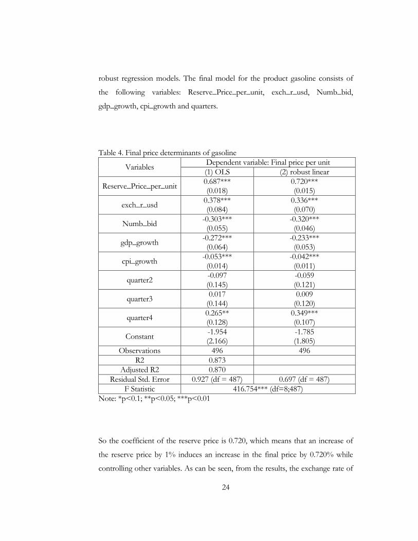
24

robust regression models. The final model for the product gasoline consists of

the following variables: Reserve_Price_per_unit, exch_r_usd, Numb_bid,

gdp_growth, cpi_growth and quarters.

Table 4. Final price determinants of gasoline

Variables Dependent variable: Final price per unit

(1) OLS (2) robust linear

Reserve_Price_per_unit 0.687*** (0.018)

0.720*** (0.015)

exch_r_usd 0.378*** (0.084)

0.336*** (0.070)

Numb_bid -0.303*** (0.055)

-0.320*** (0.046)

gdp_growth -0.272*** (0.064)

-0.233*** (0.053)

cpi_growth -0.053*** (0.014)

-0.042*** (0.011)

quarter2 -0.097 (0.145)

-0.059 (0.121)

quarter3 0.017

(0.144) 0.009

(0.120)

quarter4 0.265** (0.128)

0.349*** (0.107)

Constant -1.954 (2.166)

-1.785 (1.805)

Observations 496 496

R2 0.873

Adjusted R2 0.870

Residual Std. Error 0.927 (df = 487) 0.697 (df = 487)

F Statistic 416.754*** (df=8;487)

Note: *p<0.1; **p<0.05; ***p<0.01

So the coefficient of the reserve price is 0.720, which means that an increase of

the reserve price by 1% induces an increase in the final price by 0.720% while

controlling other variables. As can be seen, from the results, the exchange rate of

25

USD is quite significant and has a positive correlation. So an increase in the

exchange rate of USD by 1% induces an increase in the final price by 0.336%. As

is shown, this variable is influential and it is due to the dependence of the price of

gasoline in auctions on the world price for gasoline correlated with the exchange

rate of USD. In addition, the unique number of bidders matters when

participants of auction make their decisions. Thus, one more participant

decreases the final price by 0.320 UAH/unit. GDP year over year growth rate has

a positive correlation with the dependent variable. One of the reason is that GDP

can affect the level of households’ or firms’ income. Therefore, an increase by 1%

in GDP growth rate causes a decrease in the winning bid by 0.272%. The final

variable is CPI year over year growth rate. It has a negative correlation. So an

increase by 1% in CPI growth rate induces a decrease in the winning bid by

0.042%. This relation is strange as we expect that the higher the CPI growth rate,

the higher the winning bid. Besides that, the dummy for the fourth quarter

matters, so in the last quarter of a year the winning bid increases by 0.349% in

comparison with the first quarter of a year.

As a result, this model based on a given sample can explain variation in the

dependent variable by 87.3%, if we look at the corresponding OLS model. Very

similar results are obtained for other products: eggs and potato. The results for

these models are in the Appendix C.

Let us discuss the results of the model for eggs. It can be seen from the results,

there is a positive correlation between the winning bid and the reserve price, the

fourth quarter of a year and a negative correlation between the dependent

variable and the unique number of bidders, GDP year over year growth rate, CPI

year over year growth rate and the second quarter of a year. Significance of the

second and the fourth quarters means that there is a seasonality in the target

variable. Directions of changes of the final price caused by independent variables

26

are consistent with the results from the previous model. The only difference is in

the magnitude of the coefficients and the exchange rate for USD is not significant

in this model. So 1% increase in the reserve price causes an increase by 0.477% in

the final price. An increase by 1 participant in the auction changes the winning

bid by -0.096%. We see that when GDP growth rate decreases by 1% then the

last price increases by 0.355%. Also, 1% decrease in the CPI growth rate

increases the final price by 0.028%. The final significant variables are quarters. So

in the second quarter the winning bid is smaller by 0.297% and in the fourth

quarter it is larger by 0.213% in comparison with the first quarter. Thus, this

model describes the variation of the target variable by 78.8%, if we look at the

corresponding OLS model.

Finally, let us examine the model for potato. In comparison with the previous

two models, we can see that this model includes less number of independent

variables, which explain the variation in the target variable. So significant variables

are the following: the reserve price, the unique number of bidders, the second

and the third quarter of a year. Directions of changes are the same. The relation

between the reserve price and the final price for this model is the same as for the

previous model for eggs. The second variable, the unique number of bidders, has

a negative correlation and an increase by 1 participant in the auction decreases the

final price by 0.364 UAH/unit.

Eventually, the winning bid in the second quarter is higher by 0.486% and in the

third quarter is less by 0.179% in comparison with the first quarter of a year.

Thus, this model explains the variation of the dependent variable by 61.8%, if we

look at the corresponding OLS model. Three models are quite good as they have

R-squared in the range of 61.8-87.3%

27

5.2. Reserve price determinants for gasoline, eggs and potato

Now we consider the model (4) from the methodology. As a dependent variable,

we use the reserve price in the current period and as the main independent

variable, we take the winning bid in the previous period for the same buyer. The

model is on the basis of the cross-sectional data. In case of gasoline, the sample

has 439 observations.

As for the previous three models where the target variable is the final price, we

check independent variables for multicollinearity and the model for

heteroscedasticity. As a results of tests, which can be seen in the Appendix A and

B respectively, we conclude that there is no multicollinearity and there is a

heteroscedasticity in three subsequent models. We discuss only coefficients for

the robust regression models, but R-squared from the corresponding OLS

models.

After modelling the equation (4) we obtain the results shown in Table 5. As a

result of this model, we can see that an increase in the final price in the previous

period by 1% causes an increase in the reserve price in the current period by

0.578%. For this model, the exchange rate has a higher coefficient, which means

that the buyers’ decision is more based on this variable than for sellers based on

the results of the previous model.

As for the previous model for gasoline, GDP year over year growth rate is also

included into the model and has the following relation: an increase in GDP

growth rate by 1% causes a decrease in the reserve price by 1.109%. Besides that,

this model incorporates dummy variable for quarters. So the second and the third

quarter matter with a negative sign. So there is a seasonality for this model when

buyers choose the optimal initial price of the auction. Based on the results, this

model explains 63% variation in the reserve price for gasoline.

28

Table 5. Reserve price determinants of gasoline

Variables Dependent variable: Reserve price per unit

(1) OLS (2) robust linear

Final_Price_per_unit 0.516*** (0.043)

0.578*** (0.036)

exch_r_usd 0.690*** (0.170)

0.751*** (0.141)

gdp_growth -1.365*** (0.125)

-1.109*** (0.104)

cpi_growth -0.151*** (0.033)

-0.108*** (0.028)

quarter2 -1.379*** (0.287)

-1.002*** (0.239)

quarter3 -1.018*** (0.295)

-0.774*** (0.245)

quarter4 -0.009 (0.249)

0.146 (0.207)

Constant 0.667

(4.669) -3.786 (3.881)

Observations 439 439

R2 0.647

Adjusted R2 0.642

Residual Std. Error 1.761 (df=431) 1.254 (df=431)

F Statistic 113.059*** (df=7;431)

Note: *p<0.1; **p<0.05; ***p<0.01

The results for eggs and potato can be found in the Appendix D. The next model

for discussing is the model for eggs. This model has the same signs for

independent variables for the previous model above. However, the coefficient of

the final price in the previous period is much less then for other two models

where the reserve price is the dependent variable. So an increase by 1% in the

winning bid in the previous period causes an increases in the reserve price by

0.099%. The exchange rate for USD has an important part in this model and

when this variable increases by 1% then the target variable increases by 0.152%.

GDP year over year growth rate has a negative correlation as it is expected, but

29

the magnitude is quite high. So an increase by 1% in this variable induces a

decrease in the reserve price by 0.892%. Finally, quarters have an important part

in this model, as all quarters matter. The closed to the end of a year, the higher

the reserve price in comparison with the first quarter.

Eventually, the last model where the target variable is the reserve price is the

model for potato. This models includes only three significant variables, which are

the following: the final price in the previous period, CPI growth rate and the

dummy for quarters. The coefficient of the final price is quite close to the

coefficient of the similar model for gasoline. So an increase by 1% in this variable

causes an increase in the reserve price by 0.537%. Besides that, CPI growth rate

has a positive correlation with the dependent variable and an increase in this

variable induces an increase in the target variable by 0.293%. Finally, the closer to

the end of a year, the less is the reserve price. In this case, only the second and

the fourth quarters matter.

Thus, all three models described above describe the variation in the reserve price

quite good. R-squared for the corresponding OLS models are within 26.6-67.1%.

In the next section, we summarize results obtained in this study.

30

C h a p t e r 6

CONCLUSIONS

The main idea of this research is to show the allocation between the reserve price

and the winning bid in the last round of the auction. This is of interest as it can

help buyers as well as sellers while they are trying to find the best strategy in a

given situation. There are a lot of different papers about how to evaluate optimal

strategies and some of them are listed in the methodology of this paper.

Models for this research are based on the available ones from the literature and

they are modified in order to use other factors, which could have an effect on

dependent variables. The final price and the reserve price determinants are

considered in this paper. Thus, the first model is the model for estimating the

winning bid and the second model is the model where the reserve price is set to

be the dependent variable. In order to modify models macroeconomic factors are

used such as GDP year over year growth rate, CPI year over year growth rate, the

exchange rate of USD. These variables allow to extend available models in the

literature and explain better variation in the dependent variable.

For modelling, the data from biprozorro.gov are used with 1970 observations for

the period from 2016 till 2018 for below the threshold competitive auctions and

only for three products: gasoline, eggs and potato. So we have obtained similar

results for all models. In general R-squared is quite high that lies within 27-87%.

It implies that models explain variation in the dependent variable strong enough.

The first model gives the following allocation between the reserve price and the

final price. An increase of the reserve price in period t by 1% causes an increase

31

in the final price in period t by 0.5-0.7% and an increase of the final price in

period t-1 by 1% causes an increase in the reserve price in period t by 0.1-0.5%.

These results are for gasoline, eggs and potato.

In addition, models of this paper can be extended for other products as well. As

the first advice, we propose to consider other products that can have seasonality

as potato and eggs have over quarters. As the second advice for the future study

is to take more observations from ProZorro auctions or consider different types

of procedures of auctions.

32

WORKS CITED

Amidu, A.-R. and A. O., Agboola. 2009. “Empirical Evidence Of The Influences On First-Price Bid Auction Premiums,” International Real Estate Review 12 (2): 157-170. https://ideas.repec.org/a/ire/issued/v12n022009p157-170.html.

Bajari, P. and A., Hortacsu. 2003. “The Winners Curse, Reserve Prices, and

Endogenous Entry: Empirical Insights from EBay Auctions.” The RAND Journal of Economics 34(2): 329-355. https://EconPapers.repec.org/RePEc:rje:randje:v:34:y:2003:i:2:p:329-55.

Bajari, P., C. L., Benkard, and J., Levin. 2007. “Estimating Dynamic Models of

Imperfect Competition.” Econometrica 75, no. 5 (August): 1331-370. https://doi.org/10.1111/j.1468-0262.2007.00796.x.

Choi, S., I., Rasul, and L., Nesheim. 2010. “Reserve Price Effects in Auctions:

Estimates from Multiple RD Designs.” Cemmap Working Paper , (May): https://doi.org/10.1920/wp.cem.2010.3010.

Elyakime, B., J.-J., Laffont, P., Loisel, and Q., Vuong. 1997. “Auctioning and

Bargaining: An Econometric Study of Timber Auctions with Secret Reservation Prices.” Journal of Business & Economic Statistics 15, no. 2 (April): 209. https://doi.org/10.2307/1392306.

Isaac, R. M., T. C., Salmon, and A., Zillante. 2007. “A Theory of Jump Bidding in

Ascending Auctions.” Journal of Economic Behavior & Organization 62, no. 1 (January): 144-64. https://doi.org/10.1016/j.jebo.2004.04.009.

Jofre-Bonet, M. and M., Pesendorfer. 2003. “Estimation of a Dynamic Auction

Game.” Econometrica, v71 (September): 1443-1489. https://doi.org/10.3386/w8626.

Lo, K. C. 1998. “Sealed Bid Auctions with Uncertainty Averse Bidders.” Economic

Theory 12, no. 1 (July): 1-20. https://doi.org/10.1007/s001990050209. Lu, J.. 2006. Three essays on multi-round procurement auctions. Nashville,

Tennessee: Graduate School of VU. Lucking-Reiley, D., D., Bryan, N., Prasad, and D., Reeves. 2007. “Pennies from

eBay: the Determinants of Price in Online Auctions.” The Journal of Industrial Economics 55, no 2 (July): https://doi.org/10.1111/j.1467-6451.2007.00309.x.

https://econpapers.repec.org/RePEc:rje:randje:v:34:y:2003:i:2:p:329-55

33

Malisuwan, S., S., Jesada, T., Noppadol, and S., Nattakit. 2015.”Spectrum Auction Theory and Spectrum Price Model.” International Journal of Innovative Research and Development 4 (12): http://www.ijird.com/index.php/ijird/article/view/84113.html.

Reiß, J. P., and J. R., Schöndube. 2008. “First-price Equilibrium and Revenue

Equivalence in a Sequential Procurement Auction Model.” Economic Theory 43, no. 1 (December): 99-141. https://doi.org/10.1007/s00199-008-0428-7.

Roberts, J. W. 2009. “Unobserved Heterogeneity and Reserve Prices in

Auctions.” SSRN Electronic Journal 44, no 80 (October): https://doi.org/10.2139/ssrn.1695647.

Roth, A. E., and A., Ockenfels. 2002. “Last Minute Bidding and the Rules for

Ending Second-Price Auctions: Theory and Evidence from a Natural Experiment on the Internet.” American Economic Review, v92 (September): 1093-1103. https://doi.org/10.3386/w7729.

Seçkin, A. and E., Atukeren. 2012. “A Heckit Model of Sales Dynamics in

Turkish Art Auctions: 2005-2008.” Review of Middle East Economics and Finance 7, no. 3 (May): 1-32. https//doi.org/10.1515/1475-3693.1304.

Stephen, G. D., H. J., Paarsch, and J., Robert. 2006. “An Empirical Model of the

Multi-Unit, Sequential, Clock Auction.” Journal of Applied Econometrics 21, no. 8 (December): 1221-1247. https://doi.org/10.1002/jae.854.

Wan, W. and H.-H., Teo. 2001. “An examination of auction price determinants

on eBay.” The 9th European conference on information systems, 2001, 898-908. Bled: School of Computing. National University of Singapore.

34

APPENDIX A

CHECKING FOR MULTICOLLINEARITY

Figure 6. Correlation between independent variables for the model (2) for gasoline

35

Figure 7. Correlation between independent variables for the model (2) for eggs

Figure 8. Correlation between independent variables for the model (2) for potato

36

Figure 9. Correlation between independent variables for the model (4) for gasoline

Figure 10. Correlation between independent variables for the model (4) for eggs

37

Figure 11. Correlation between independent variables for the model (4) for potato

38

APPENDIX B

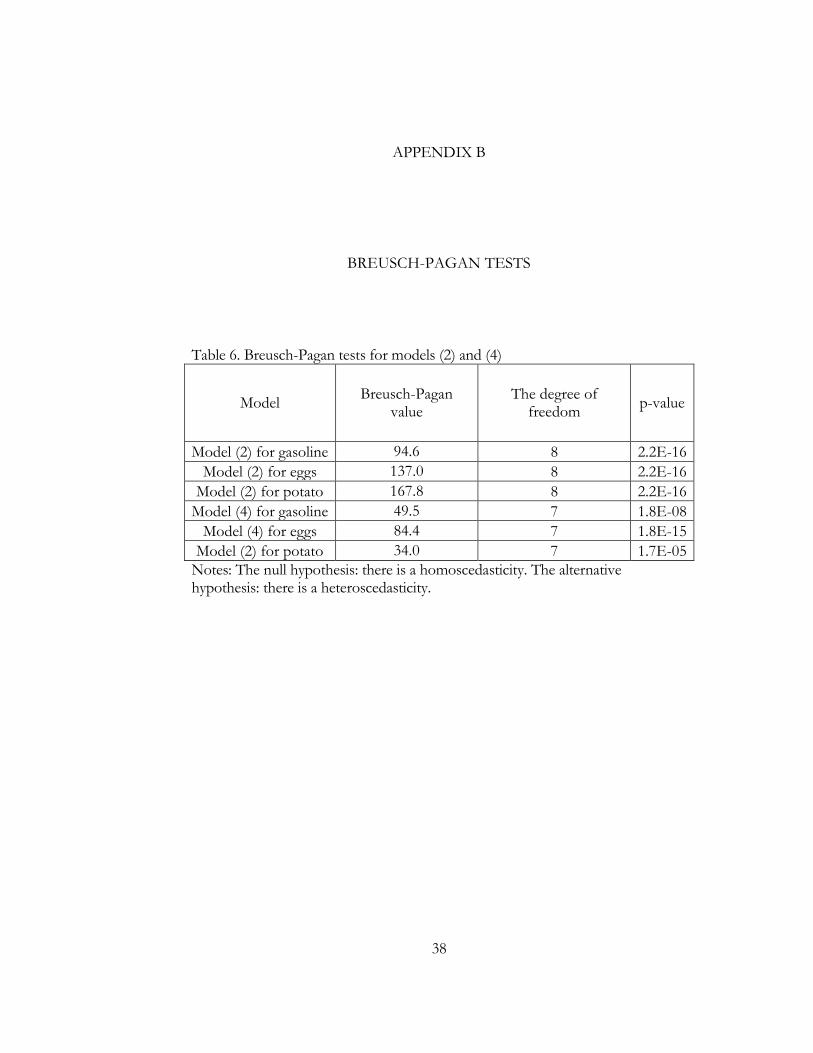
BREUSCH-PAGAN TESTS

Table 6. Breusch-Pagan tests for models (2) and (4)

Model Breusch-Pagan

value The degree of

freedom p-value

Model (2) for gasoline 94.6 8 2.2E-16

Model (2) for eggs 137.0 8 2.2E-16

Model (2) for potato 167.8 8 2.2E-16

Model (4) for gasoline 49.5 7 1.8E-08

Model (4) for eggs 84.4 7 1.8E-15

Model (2) for potato 34.0 7 1.7E-05

Notes: The null hypothesis: there is a homoscedasticity. The alternative hypothesis: there is a heteroscedasticity.

39

APPENDIX C

EMPRICAL RESULTS FOR THE MODEL (2) FOR EGGS AND POTATO

Table 7. Final price determinants of eggs


(1) OLS (2) OLS (3) robust linear


0.481*** (0.024)

0.477*** (0.023)

exch_r_usd 0.008

(0.017)

Numb_bid -0.098*** (0.010)

-0.097*** (0.010)

-0.096*** (0.009)

gdp_growth -0.315*** (0.025)

-0.317*** (0.025)

-0.355*** (0.023)

cpi_growth -0.026*** (0.011)

-0.026*** (0.011)

-0.028*** (0.010)

quarter2 -0.317*** (0.036)

-0.322*** (0.035)

-0.297*** (0.033)

quarter3 -0.045 (0.041)

-0.053 (0.038)

-0.037 (0.036)

quarter4 0.224*** (0.026)

0.223*** (0.026)

0.213*** (0.025)

Constant 1.777*** (0.507)

1.998*** (0.202)

2.104*** (0.193)

Observations 797 797 797

R2 0.789 0.788

Adjusted R2 0.787 0.786

Residual Std. Error 0.251 (df=788) 0.251 (df=789) 0.225 (df=789)

F Statistic 367.892*** (df=8;788)

420.829*** (df=7;789)

Note: *p<0.1; **p<0.05; ***p<0.01

40

Table 8. Final price determinants of potato




0.472*** (0.017)

0.477*** (0.023)

exch_r_usd 0.112

(0.072)

Numb_bid -0.381*** (0.038)

-0.383*** (0.038)

-0.364*** (0.034)

gdp_growth -0.005 (0.117)

cpi_growth 0.061* (0.036)

quarter2 0.519*** (0.136)

0.392*** (0.114)

0.486*** (0.101)

quarter3 -0.194 (0.136)

-0.206** (0.098)

-0.179*** (0.087)

quarter4 -0.137 (0.098)

-0.130 (0.097)

-0.076 (0.086)

Constant -1.125 (2.197)

2.753*** (0.172)

2.633*** (0.153)


R2 0.621 0.618

Adjusted R2 0.616 0.615


F Statistic 136.749*** (df=8;668)

217.148*** (df=5;671)

Note: *p<0.1; **p<0.05; ***p<0.01

41

APPENDIX D

EMPRICAL RESULTS FOR THE MODEL (4) FOR EGGS AND POTATO

Table 9. Reserve price determinants of eggs




0.118** (0.046)

0.099*** (0.037)

exch_r_usd 0.124*** (0.034)

0.129*** (0.033)

0.152*** (0.027)

gdp_growth -0.701*** (0.070)

-0.708*** (0.069)

-0.892*** (0.056)

cpi_growth -0.036 (0.032)

quarter2 -0.486*** (0.084)

-0.459*** (0.081)

-0.361*** (0.065)

quarter3 -0.200** (0.094)

-0.261*** (0.078)

-0.173*** (0.062)

quarter4 0.139** (0.055)

0.152*** (0.054)

0.161*** (0.044)

Constant 0.705

(1.106) 0.051

(0.945) -0.252 (0.761)


R2 0.672 0.671

Adjusted R2 0.665 0.665


F Statistic 95.097*** (df=7;325)

110.634*** (df=6;326)

Note: *p<0.1; **p<0.05; ***p<0.01

42

Table 10. Reserve price determinants of potato




0.514** (0.074)

0.537*** (0.068)

exch_r_usd -0.047 (0.208)

gdp_growth -0.396 (0.517)

cpi_growth 0.272** (0.127)

0.300*** (0.121)

0.293*** (0.112)

quarter2 2.141*** (0.551)

1.947*** (0.422)

1.939*** (0.390)

quarter3 -0.160 (0.556)

-0.361 (0.409)

-0.565 (0.378)

quarter4 -0.681*** (0.327)

-0.751** (0.311)

-0.659** (0.287)

Constant 2.676

(6.152) 0.365

(1.693) 0.264

(1.564)


R2 0.267 0.266

Adjusted R2 0.248 0.252


F Statistic 13.866*** (df=7;266)

19.390*** (df=5;268)

Note: *p<0.1; **p<0.05; ***p<0.01

RESERVE PRICE DETERMINANTS IN PROZORRO AUCTIONS IN … · ProZorro auctions. The main objective of...

Documents

Transcript of RESERVE PRICE DETERMINANTS IN PROZORRO AUCTIONS IN … · ProZorro auctions. The main objective of...