Research Report Department of Statistics G6teborg University Sweden

Mailing address: Department of Statistics Goteborg University 5-411 80 Goteborg Sweden

Evaluation of univariate surveillance procedures for some multivariate problems

Peter Wessman

Fax Nat: 031-7731274 Int: +4631 773 12 74

Research Report 1996:4 ISSN 0349-8034

Phone Home Page: Nat: 031-77310 00 http://www.stat.gu.se Int: +46 31 773 1000

Evaluation of univariate surveillance procedures

for some multivariate problems.

Peter Wessman Department of Statistics, Goteborg University.

S - 411 80 Goteborg.

ABSTRACT

The continual surveillance to detect changes has so far received large attention in the area of industrial quality control, where the monitoring of manufacturing processes to detect decreases in quality play an important role. However, also in other areas important examples can be found such as the surveillance of intensity care patients or the monitoring of economic trends.

Often more than one measurement is made, resulting in a multivariate obser­vation process. Many surveillance procedures for multivariate observation pro­cesses are based on summarizing statistics that reduces the multivariate process to a univariate process. This thesis studies such surveillance procedures when a change to a specific alternative is of interest. We give special attention to pro­cedures based on likelihood ratio statistics of the observation vectors since these are known to have several optimality properties. Also, many procedures in use today can be formulated in terms of likelihood ratios.

In report I we consider the surveillance of a multivariate process with a com­mon change point for all component processes. We show that the univariate reduction using the likelihood ratio statistic for the observation vector from each observation time is sufficient for detecting the change. Furthermore, the use of a likelihood ratio-based method, the LR method, for constructing surveillance procedures is suggested for multivariate surveillance situations. The LR proce­dure, as several other multivariate surveillance procedures, can be formulated as univariate procedures based on the univariate process of likelihood ratios. Thus, evaluating these multivariate surveillance procedures which are based on this re­duction can be done by using results for univariate procedures, for example those given in report II. The effects of not using a sufficient univariate statistic is also

illustrated.

In the second report a simulation study of some methods based on likelihood ratios of univariate processes is made. The LR method and the Roberts procedure are compared with two methods that today are in common use, the Shewhart and the CUSUM methods. Several different measurements of performance are used, such as the probability of successful detection, the predictive value and the expected delay of an alarm. The evaluation is made for geometrically distributed change points. For this situation the LR procedure meets several optimality cri­teria and is therefore suitable as a benchmark. The LR procedure is shown to be robust against misspecifications of the intensities. The CUSUM method ap­pears in the simulations to be closer to the Shewhart method than to the Roberts method in several of the properties investigated, for example the run length dis­tribution and the predictive value. Furthermore, the Roberts procedure is shown to have properties close to the LR procedure for moderately large intensities. It has therefore near optimal properties in these cases.

This thesis consists of two parts:

I Some principles for surveillance adopted for multivariate processes with a com­mon change point.

II Evaluations of likelihood ratio methods for surveillance.

ACKNOWLEDGEMENT

I would like to thank my supervisor, Professor Marianne Frisen, for her sup­port and guidance throughout this work. I also wish to thank my collegues and friends at the Department of Statistics, especially Aila Sarkka and Goran Akermo for their valuable comments on the draft manuscript.

11

Some principles for surveillance adopted for multivariate processes

with a common change point.

Peter Wessman Department of Statistics, University of Goteborg,

S - 411 80 Goteborg.

Abstract

The surveillance of multivariate processes has received growing at­tention during the last decade. Several generalizations of well-known methods such as Shewhart, CUSUM and EWMA charts have been proposed. Many of these multivariate procedures are based on a uni­variate summarized statistic of the multivariate observations, usually the likelihood ratio statistic. In this paper we consider the surveil­lance of multivariate observation processes for a shift between two fully specified alternatives. The effect of the dimension reduction using likelihood ratio statistics are discussed in the context of suf­ficiency properties. Also, an example of the loss of efficiency when not using the univariate sufficient statistic is given. Furthermore, a likelihood ratio method, the LR method, for constructing surveillance procedures is suggested for multivariate surveillance situations. It is shown to produce univariate surveillance procedures based on the suf­ficient likelihood ratios. As the LR procedure has several optimality properties in the univariate, it is also used here as a benchmark for comparisons between multivariate surveillance procedures.

Key words: Multivariate surveillance, sufficiency, Likelihood ratio, CUSUM.

1

1 Introduction

The surveillance of random processes to detect a change has received much attention during the last decades. Contributions have been made especially in industrial quality control, but also in other areas such as medicine, epi­demiology or economy. The term surveillance is mainly used in the medical and epidemiological fields. Other names for this type of problem are moni­toring, change point detection or statistical process control.

In surveillance the process is continually observed through a sequence of observations made continuously or at specific intervals. These observations can be either the original measurements or a function of these, for example the mean of a sample from each time point. Whenever the process is observed through more than one observation sequence we have a multivariate surveil­lance situation. Consider for example the monitoring of a manufacturing process to detect decreases in the product quality. In this situation several measurements are often taken simultaneously. For example, the quality of a product can be defined through several different attributes or there may be parallel lines of production monitored independently. In other cases the process is observed at different stages in the production.

When the surveillance starts the process is considered in control with observations from a known and acceptable distribution. At some unknown random time point a change occurs in the process, resulting in a change in distribution of the observations. This change usually consists of a change in the parameter vector either to a specific new point or a general shift away from the in-control parameter vector. The observation sequence is usually assumed to be independent, both before and after the change, and to have a well known distribution family such as the Gaussian family.

Of primary interest in surveillance is the random change point where a change occurs. Based on the observation process a decision must be made after each time point whether or not an event has occurred. To do this, an alarm-procedure of some sort is used. Examples of well-known procedures for univariate observation processes include the Shewhart, CUSUM and EWMA procedures, see for example Whetherill and Brown (1991).

In multivariate surveillance situations the change in the underlying pro­cess, depending on the way it is measured, can affect the observations differ­ently. For example, if the quality in the example above depends only on the

2

raw materials used, then the change points in the different lines are likely to occur simultaneously in the case when parallel production lines are moni­tored. If instead the quality is measured at different stages of the production line then the change points for the different observation sequences differ, de­pending on what stage they are taken.

Multivariate surveillance has received an increased interest during the last decade with many new alarm procedures suggested. There are several situations that have earlier been treated as univariate ones but where a mul­tivariate perspective might be useful. For examples in the post marketing surveillance of medical drugs, Svereus (1995), where normally several dif­ferent adverse events are monitored simultaneously or in the monitoring of economic trends, Frisen (1994), where several economic indexes are used. Another area where multivariate surveillance approach may be of use is in the surveillance of ecological systems, Pettersson (1996).

The alarm procedures for surveilling multivariate observation processes can be divided into those using some univariate procedure based on a sum­marizing statistic of some kind and others, for example those where the com­ponent processes are monitored separately. In this paper we discuss some properties, such as the sufficiency property, and compare the two types of procedures. We will also suggest a type of likelihood ratio-based surveillance procedure shown to have certain optimality properties. We restrict our at­tention to processes where a sudden shift occurs between two fully specified alternatives. A consequence of this limitation is that only situations where the change occurs simultaneously in all components processes are considered.

In Section 2 we will give a more formal definition of the multivariate surveillance problem with some limitations and assumptions made in this paper. We shall also mention shortly some useful measurements of perfor­mance. Section 3 contains a short review of the literature on multivari­ate surveillance and a description of some types of alarm procedures. In Section 4 we consider the effect of using a summarizing statistic to reduce the observation-vector to a univariate observation sequence. We discuss the likelihood ratio-based multivariate surveillance procedures in Section 5. A summary and some conclusions are finally given in Section 6.

3

2 Preliminaries

2.1 Specifications and Notation

In multivariate surveillance the process of interest is observed through a p-dimensional vector

X(t) = (Xl:(t) ) ,t = 1,2, ...

Xp (t) (1)

of observations. These observations, either the original measurement or transformations of these, are considered independent, with some distribution F (t). At unknown random time points, 717"', 7p , a change occurs in the different component processes, thus in multivariate surveillance the random change point is a random vector

r=(J (2)

of change points. Depending on the application of interest the structure of this vector assumes different forms. The change in the underlying process can affect the component change points simultaneously, with deterministic delays for some components, or stochastically, where the change point of each component has some distribution GTi'i = 1, ... ,po We shall here consider only the special case with one simultaneous change point, Ti = 7, i = 1, ... ,p, for all component processes following some distribution GT' In some sections, GT is specified to be the geometric distribution with intensity v. This is the most commonly used assumption in the theoretical literature and it is also a reasonable assumption in many practical applications. Some useful results for this case can be found in for example Shiryaev (1963).

In addition to a common change point for component processes we also assume that there exist two fully specified alternatives. Thus, we consider an observation process X with distribution FO for all X (1) , X (2) , ... , X (7 - 1) and Fl for X (7) , X (7 + 1) , ....

As mentioned above we are primarily interested in a sequence of crit­ical events concerning 7. Usually we are interested in detecting a change whenever it has occurred. However, sometimes only some of the possible change points of interest at each time s are of interest, for example we might only be interested in detecting a change that has occurred in the latest d observation points. We therefore define two events in the sample space of

4

7, C (s) = {7 E Is ~ {1, ... , s}}, the set of time points where we, at time s, want to detect a change, and D (s) = {7 > s}, where no change has yet oc­curred at time s. It should be noted that D (s) is not always the complement event of C (s). In fact, only if C (s) = {7 ::; s}, that is we are interested in detecting a change occurring at any possible change point up to time s,is D (s) the complement event.

A surveillance procedure can be defined through a stopping time tA, which determines when an alarm should be given. We can define the stopping time through an alarm function P (.; C (s)) and a critical limit K (s) as

t A = min [s; P (Xs; C (s)) > K (s) ] . (3)

or through the alarm set

A (s) = {xs E Slx.lp (xs; C (s)) > K (s)} (4)

of outcomes leading to an alarm. The critical limit K (s) regulates the prob­abilities of making a (false) alarm and the alarm function P (.) is a function of the available information at time s, Xs = {X (1) , ... , X (s)} E Slx., ( and possibly also of G r ). Note the different use of the index in Xi and Xi (t), the former indicating a truncated sequence and the latter the observations made at time t of component process i. A simple example of an alarm function is the alarm function for the Shewhart chart P (xs ; C (s)) = x (s). Using only the latest observation, the Shew hart procedure is designed to detect the particular critical event C (s) = {7 = s}.

2.2 Measurements of Performance

The performance of a procedure can be studied through the relationship be­tween the change point 7 and the stopping time tAo To be able to construct, or choose between, surveillance procedures some measure of performance or criterion of optimality is necessary.

Two important properties for a surveillance procedure are: i) that the procedure should have a high probability to detect a change and do so within reasonable time and ii) the procedure should have a low probability for a false alarm. These two properties are unfortunately in conflict with each other, as for example a lower false alarm probability will usually give a lower probability of detecting a change. The desirable properties differ between applications and some sort of measurement of the performance of a procedure is therefore useful.

5

One measurement of performance dealing with the balance between the two properties i) and ii) is the Predictive Value, Frisen (1992). This is defined as

Pr (tA = t,T::; t) PV(t) = Pr(T < t ItA = t) = Pr(tA = t,T::; t) + Pr(tA = t,T > t)' (5)

t = 1,2, ... , and measures the balance between motivated and unmotivated alarms, giving a measure of the confidence we can have in an alarm given at a certain time. Other measurements are concerned with just one of these two properties. For example, the average run length, ARL, where ARLO := E [tA IT = 00], the ARL when no change occurs, deals with prop­erty ii) and ARLI = E [tA IT = 1] deals with property i).

In quality control the most commonly used measure of performance is the ARL where a procedure is sometimes considered optimal if it minimizes the ARLI for fixed ARLo. The limitations of this optimality criterion have been discussed by Akermo, (1995) and Frisen (1996).

Another way of defining an optimal procedure is by:

Definition 2.1 If A ~ Ox. is an alarm set, e a critical event concerning T

and D a proper subset of the complement of e, then A is the optimal alarm set if for all B ~ Ox.;

Pr (B Ie) > Pr(A Ie) ~ Pr (B ID) > Pr (A ID) (6)

Thus the procedure is deemed optimal if any other surveillance procedure with higher probability to detect a change also has a higher probability of giving a false alarm.

Shirayev (1963) defined optimality, S-optimality, using the speed of de­tection and the false alarm rate. He defined the optimal alarm procedure as the one with minimal expected cost, for a specific cost function of the delay of an alarm and a false alarm.

3 A Short Review of Literature and Meth­ods

During the last decade several new procedures for surveilling multivariate ob­servation processes have been suggested. Most of them are generalizations of

6

procedures developed for monitoring univariate observation processes. How­ever, a common approach is still to monitor each component separately, usually using a union intersection type of procedure, Hochberg & Tamhane (1987), to decide on an alarm. A simple example is the union intersection Shewhart procedure, (VI Shewhart), where an alarm is made whenever one component exceeds its predefined limit.

The first one to consider the surveillance of several observation processes as a multivariate problem seems to have been Hotelling (1947). He suggested the monitoring of a shift in the mean of a multivariate Gaussian process using a Shewhart procedure based on a summarizing statistic, the so-called T2 - statistic:

I

T2 (t) = (x (8) - J-L0) ~-l (x (8) - J-L0

) ,t = 1,2,... (7)

where J-L0 is the in-control mean and ~ is the covariance matrix. When ~ is known the procedure is called the Shewhart X2 -chart. Further development of procedures based on the Shew hart chart has been done, for example using principal components, Alt (1985).

Several different generalizations of the CVSVM procedure based on the T2_ statistic have also been suggested, see for example Pigniatello & Runger (1990), Alwan (1986) and Crosier (1988). These are, as the Shewhart X2 pro­cedure, directionally invariant and constructed to detect shifts in the mean vector in any direction.

In recent years also generalizations of exponential weighted moving aver­age procedures, EWMA, have been made. For example Lowry et al. (1992) proposed the use of Z (t) = RX (t) + (I - R) Z (t - 1) ,t = 1,2, ... , where Z (0) = 0 and R = diag (rl,"" rp) and to signal an alarm when

{ 2-r I } min t; -r-Z (t) ~-lZ (t) > K e

• (8)

Thus, also this procedure is based on the T2 statistic and directional invari­ant for changes in the mean vector.

Woodal and Ncube (1985) used the principal components of the observa­tions when they suggested a union intersection type of procedure based on univariate CUSVM charts, one for each independent principal component. The stopping time for the CVSUM procedure they used is defined as

min {t; max (0, Si (t - 1) + Xi (t) - ki) > hi} ,i = 1, ... ,p, (9)

7

with 0 ::; Si (0) < hi' The reference value, ki ~ 0 and the critical limit hi are chosen for each component process so that the change can be detected quickly.

Other examples of procedures to monitor changes to a specific alternative using summarizing statistics are more rare. One example is the procedure suggested by Healy (1987) which will be discussed later in section 4. Hawkins (1991 and 1993), considering monitoring of regression adjusted variables, has extended Healy's work to the surveillance of a set of specified alternatives.

4 Summarizing Statistics in Surveillance Pro­cedures of Multivariate Processes

4.1 Sufficiency

Many of the suggested surveillance procedures proposed so far for monitoring multivariate processes are based the univariate likelihood ratios of the ob­servation vector from each observation time point. This raises the question of possible information loss caused by using the likelihood ratio statistic to reduce the dimension of the multivariate process. It is therefore of interest to see if the use of the likelihood ratio statistic is sufficient for detecting the change. Following Cox & Hinkley (1974) we define sufficiency as:

Definition 4.1 A statistic T is sufficient for a family of distributions F if and only if the conditional density fXIT (x It) is the same for all F E F. In addition, a sufficient statistic is said to be minimal sufficient if no sufficient statistic of lower dimension can be found.

Since we are here interested in sequential decisions a definition of suffi­ciency of a sequence of statistics is also useful. Following Arnold (1988) we define this as:

Definition 4.2 A sequence Tl (XI) , T2 (X2) , ••• of statistics is a sufficient sequence of statistics for the families F1, F2, ... of distributions if for all s, Ts (Xs) is a sufficient statistic for the family Fs.

Consider as before a surveillance situation where we monitor a process through a sequence, X = {X (t) ; t = 1,2, ... }, of independent observations for which a change in the process introduces the shift in the distribution:

{ FO

X (t) rv F (t) = Fl

8

T > t T::;t' (10)

where FO and Fl are two completely specified distributions. Notice that when considering this type of change we also assume a simultaneous change point 7 for the component processes.

The available information Xs = (X (1) , ... , X (s)) for a decision between the events C (s) = {7 ::s s} and D (s) = {7 > s} has, at time s, a distribution from the family:

(11)

Thus the decision whether or not a change has occurred , based on the observations sequence {X (t) ; t = 1,2, ... }, can be formulated as a decision between whether Xs has a distribution from the family FD(s) or Fe(s). We therefore want to find a statistic Ts (Xs) that is sufficient for the family {FC(S) , FD(S)} for each s, thus making the sequence {Ts (Xs) ; s = 1,2, ... }

a sufficient sequence of statistics for the sequence {Fe(s), FD(s); s = 1,2, ... }. We prove the following statement.

Statement 4.1 For the model 'above with 7i = 7, i = 1, ... ,p the univariate process {l r (x (t)) ; t = 1, 2, ... } of likelihood ratios, as defined below, is a sufficient reduction of the multivariate observation process for the sequence of families {Fe(S), FD(s); s = 1,2, ... }.

Proof: Let us first define lr (x (t)) = j1 (x (t)) / jO (x (t)) and lrdxs) = {lr (x (t)) , ... , lr (x (s))).

(i) Let 7 be fixed. Then, at time s, we can write the density of Xs as:

t-l s s s j1 (x (i)) fs (xs 17 = t) = g f O

(x (i))!! fl (x (i)) = g r (x (i))!! fO (x (i))

s

= h (xs) IT lr (x (i)) = h (xs) k (lrt (xs)) , (12) i=t

where hand k are two real valued functions. We also use the definition 11i=S+1 = 11?=1 = 1. The factorization theorem gives that the vector lrl (xs )

is sufficient for the distribution family of Xs defined by the parameter 7.

(ii) If 7 is stochastic with some distribution Gr then the density of Xs at time s can be written:

00

fs (xs) = Lgr (t) fs (xs 17 = t) t=l

9

= h (xs ) [~gr (t) k (lrt (xs )) + (1 - Gr (t)) k (lrl (xs ))] (13)

and again using the factorization theorem we have that lrl (x s) is sufficient for the family {FC(s), FD(s) }.

(iii) Finally, since lrl (xs ) is sufficient for any s, we have according to def­inition 4.2 that the sequence {lrl (xs ) ; S = 1,2, ... } is a sufficient sequence for the sequence of families {FC(s) , FD(s); S = 1,2, ... }. Thus to monitor for a simultaneous, fully specited, shift in a multivariate observation process it is possible to construct a univariate surveillance procedure based on the sufficient sequence of likelihood ratios. 0

For the surveillance of a univariate observation process there exists in gen­eral no sufficient statistic of a lower dimension than the sample itself. Thus, a procedure based on {lrl (x s ) ; S = 1,2, ... } = {Ir (x (t)) ; t = 1,2, ... } is in these cases also minimal sufficient. For example in the case with observa­tions of a univarite Gaussian distribution there is no sufficient statistic with a lower dimension than the sample itself, see Cox and Hinkley (1974, p.30).

4.1.1 Sufficient Reduction for Observation from a k-Dimensional Exponential Family

Most procedures proposed so far in literature have been constructed for ob­servations from the exponential family. We consider observations from such a k-dimensional exponential family where we are monitoring for a shift in the parameter vector between two (natural) parameter vectors 0° and Ol;

o (t) = { ( 01, ... , op T ~ t . (14 ) (Ol'··· ,Ok) T < t

According to statement 4.1 we have that it is enough to monitor the univari­ate process of likelihood ratio statistics for observations from the exponential family;

k

Ir (t) = E (OJ - OJ) Tj (x (t)) = E (OJ - OJ) Tj (x (t)) (15) j=l j:oJ#J

where Tj (x (t)) is the minimal natural sufficient statistic for OJ.

From this follows that when surveilling a process of multivariate Gaussian distributed observations for a sudden shift in the mean vector

(

Jll (t) ) Jl (t) = : = {

/1p (t)

10

JlO = 0 T > t Jll = Jl T ~ t

(16)

with a constant covariance matrix E, then it is sufficient to monitor the sequence of likelihood ratio statistics TJl. (x (t)) = {JL'E-lx (t) ; t = 1,2, ... }. Thus, we have that the statistic is simply a weighted sum of the observations. In the case with standardized bivariate observations with a correlation p where unit shifts are of interest this statistic reduces to

TJl. (x (t)) = Xl (t) + Xz (t) l+p

If instead a shift in the covariance is monitored:

the minimal sufficient process to monitor would be

(17)

(18)

if the matrix (Eo 1 - Ell) is not singular. Notice for example that if El = eE, e a scalar, then the sufficient statistic to monitor is

TE (x (t)) = ((e - 1) Ie) (x (t) - JL)' Eol (x (t) - JL).

Thus, we have that procedures based on monitoring the Hotelling TZ-statistic are sufficient for surveilling a proportionate shift in the covariance matrix of the observation process.

4.2 Evaluation of Efficiency

In the previous subsection we saw that {lrl (xs) ; s = 1,2, ... } is sufficient for detecting C (s) = {T ::; s}. In this subsection we shall give an example of the loss of efficiency that can occur with a surveillance procedure that is not based on a sufficient reduction. We will compare two procedures based on the Shewhart chart, a univariate Shewhart procedure on the likelihood ratio statistic and a UI-Shewhart procedure based on the principal components of the observations.

Several authors have suggested the use of principal components of the observations, e.g. Jackson & Bradley (1966), Woodall & Ncube (1985) and Hawkins (1991). The reason for using principal components is usually to reduce the dimension but it is also used as a mean to transform the observa­tion vector in to a vector of independent components. We base our parallel Shewhart chart on the principal component process instead of the original data as a mean to simplify calculations.

11

As we consider Shewhart type procedures we restrict our evaluation to the use of average run length as a measure of performance. We define effi­ciency in terms of minimal the ARLI for fixed ARLo.

Let us observe a bivariate Gaussian sequence for a sudden shift in the mean with the covariance structure remaining unchanged. We can then with­out loss of generality consider the standardized process

1 ~ ~ 1 P II N2 0, P 1 7> t X (t) rv 1 p ,t = 1,2, ...

N2 11, P 1 7 ~ t (20)

with p ~ 0, for negative correlation we instead observe (Xl (t), -X2 (t))T. I

Furthermore we here consider only equal sized shifts, 11 = (11, 11)' Then the principal components

Y (t) = ~AX (t) = ...!:...- ( Xl (t) + X2 (t) ) v'2 v'2 Xl (t) - X2 (t)

(21)

are distributed

1'>t (22)

Notice that in this case all information concerning the shift is found in the first principal component. The normalized lr - statistic is in this case

and it is distributed as

{ N (0,1)

Z(t)rv N(~,1) 1'>t 1'~t

(23)

(24)

Setting m = 11 (I!P - v'2) and s = v'1+P we can see that s (Z (t) - m) = YI ·

To compare the two procedures we need to set their limits so that their ARLO equals some value "( E Z+. To set the limit for the procedure based on the lr-statistic is simple as the only limit satisfying ARLO = "( is K (s) = K =

<I?-l (1~1). The parallel procedure is more complicated since the ARLO de­pends on two critical limits, KI and K 2 . For a pair of limits to fix ARLO to

12

, the condition ARLo = 1/ (1 - FO (Kl, K 2)) = , has to be satisfied. As we are surveilling independent Gaussian variables this condition is equivalent to

(25)

Thus we have no unique pair of critical limits to fix ARLo. The possible choices of limits are

The parameter p influences the amount of interest we put in each process.

ARL1

5

4

3

2

o -1.0

----

-0.5

----------'-~- -------. ...... ,'-"' ..... ,...-- ------

- p=O p=O.25 --- p=O.5 -- p=0.75

0.0 0.5 1.0

Figure 1: The effect of the choice of critical limits, (Kl (p), K2 (p)), on ARLI for a UI Shewhart procedure. Shown for different values of the correlation, p.

If we choose p = 0 only the first component is surveilled. Our choice of p influences ARLl: for p = 1, ARLI equals ARLo and as p '\J 0 decreases monotonically. In Figure 1 the effect of some choices of p with fixed ARLo = 11 is shown. Thus the most efficient or optimal choice of critical limits in our case is to use (Kl (0), K2 (0)). In practice this is equivalent to monitor only the first principal component, Y1 (t) ,t = 1,2, ... , as was suggested by Jackson and Muldholkar (1979). Thus the optimal "parallel" Shewhart procedure here is the univariate Shew hart chart based on the likelihood ratio statistic {lrl (xs) ; s = 1,2, ... }.

13

5 A Likelihood Ratio Based Procedure

5.1 The General method

In this section we discuss the use of a method to construct surveillance pro­cedures when a specific alternative is of interest,discussed Frisen and deMare (1991), in the case of multivariate processes. As before we will consider sud­den simultanous shifts in all component processes between two fully specified alternatives. The method, here called the alarm method, constructs likeli­hood ratio based surveillance procedures designed for specific critical events and change point distributions.

The LR-procedures uses alarm functions of the form

dPr(xs IG(s)) p(xs ; G(s)) = dPr(x

s ID(s)) (27)

and give an alarm whenever this function exceeds a critical limit K(s). This critical limit usually depends both on the time of decision, s, and the distri­bution of the change point, GT • Depending on the critical event the alarm functions assume different forms. If for example we are interested in opti­mizing the procedures to immediate detection of a change, G (s) = {'T = s}, the alarm function reduces to

(28)

where f O and j1 are the densities of X (t). Thus, with K(s) = K we have the Shewhart procedure based on the likelihood ratio statistic used in section 4.2.

If instead we are interested in optimizing for the critical event G (s) = {'T :::; s}, the method results in an alarm function that can be written as

(29)

With 9T and GT being the density and distribution function of the change point 'T. A choice of critical limits with good properties is here K (s) = k· (1 - GT (s)) fGT (s), where k is a constant, as the LR-procedure is then equivalent to the procedure suggested by Shiryaev (1963).

To specify the LR procedure we need here, beside the distributions of the observations, also some knowledge of the distribution of'T. The choice of distribution for 'T is often the geometric distribution. It involves only one parameter, the intensity v, and assumes equal probability of a change in each

14

point. As 1/ -+ 0 the procedure's dependence on the choice 1/ decreases so in many practical applications where 1/ is small the specific choice of 1/ is less important, Frisen and Wessman (1996). Also when 1/ -+ 0 the alarm function has the limit

• S S j1(x(t)) hmp(xs ; {T ~ s}) = L: II fO ( ()) = Pr (xs ). (30) v-tO k=l t=k x t

thus the LR-procedure has in this case the alarm function of Roberts (1966) as its limit.

Thus, we have that the LR-procedure (29), as well as the Shewhart and the Roberts (28,30) are all based on the sequence {ir (x (t)) , t = 1,2, ... }, which is sufficient for the family {C (s) = {T ~ s} , D}. They have therefore the same optimality properties for this situation (as the respective univariate surveillance procedure).

The LR-procedure for example is of course optimal according to defi­nition 2.1 and satisfies several other optimality properties, see for example Frisen and Wessman (1996). These properties make the LR-procedure a good benchmark in theoretical or simulation studies for the multivariate surveil­lance problem discussed here. For univariate surveillance situations it has been used in this capacity by for example Frisen (1992,1996).

5.2 Surveillance of Multivariate Gaussian processes

A well-studied example in multivariate surveillance is that of a shift in the mean vector of a Gaussian process when the covariance, E, is known and stable throughout the surveillance. Without loss of generality we can con­sider shifts between flo = (0, ... ,O)T and fll = (fll, ... 'flp)T. The sufficient likelihood ratio statistic, ir (t), is then, after normalizing,

and is distributed

{ N (0, 1)

~(X(t))fV N(JK,l) T>t T~t

(31)

(32)

We can note that although the ir-statistic is here constructed for a shift to a specific point it has the same properties to detect a change to all points

15

in the parameter space satisfying {J.L* \J.L'E-1J.L* = J.L'E-1J.L}. Also, for all

shifts to points {J.L* \J.L'E-1J.L* > J.L'E-1J.L} we have that ~(x*(s)) D ~(x(s))

before a shift and, since the shift is of size J J.L'E-IJ.L* > ...;;5., we have that D

~(x*(s)) ~ ~(x(s)) after a shift. Thus, for these points we have better prop-erties for detecting the shift. A multivariate surveillance procedure based on {~(x (t)); t = 1,2, ... } for detecting a specific alternative mean vector has equal or better properties for monitoring a shift to a subspace of the param­eter space.

The LR alarm function derived for the critical events mentioned above becomes

(33)

and

(34)

respectively. The Roberts surveillance procedure consequently becomes

s s Pr (xs) = 2: II ev'Ll~(x(t))-t~ (35)

k=l t=k

Also, for the situation considered in this section Healy (1987) showed that the CUSUM-procedure

( ( J1 (x (t))) ) s (xs) = max S (Xs-l) + log fO (x (t)) ,0 . (36)

can, after normalizing, be written as

S (xs) = max (s (xs-d + ~ (x (t)) - ~-v"E, 0) . (37)

Thus, all four multivariate surveillance procedures considered here are re­duced to univariate surveillance procedures based on the univariate Gaus­sian process {~(x (t)); t = 1,2, ... }. We can therefore compare them using results for the surveillance of the mean of a univariate Gaussian process, for example a change in distribution between N (0, 1) and N (1,1). Such a comparison can be found in Frisen and Wessman (1996).

16

6 Conclusions

In many multivariate surveillance applications detection of changes in a spe­cific direction is of interest. It is sometimes of interest to construct a method with good properties to detect a change between two fully specified alter­natives, one before and one after the change, for the case when the change points occur simultaneously. We have shown that in these cases observing the univariate likelihood ratio statistic of the observations made at each time is sufficient for detecting the critical event C (s) = {1" ~ s}. In some cases it is also minimal sufficient. A good choice of surveillance procedure is therefore one based on this univariate process since the loss in efficiency when using a procedure not based on a sufficient reduction can be large, as was shown in section 4.2.

A multivariate surveillance procedure constructed by the LR-method is here shown to be equivalent to the surveillance procedure for the surveil­lance of a univariate process and to retain any optimality properties shown for univariate surveillance situations. The procedure is therefore a good candidate both as a surveillance procedure and as a benchmark in compar­isons between different multivariate surveillance procedures. We also show that comparisons between the Shew hart , the CUSUM, the Roberts and the LR-procedure are especially simple when multivariate Gaussian observation processes are considered. Such results can be found in for example Frisen & Wessman (1996).

17

References

[1] Alt, F. B. (1985). Multivariate quality control, Encyclopedia of Statis­tical Sciences. eds. Kolz, S & Johnson N. L. New York: John Wiley & Sons.

[2] Arnold, Steven F. (1988). Encyclopedia of Statistical Science. eds. Kolz, S & Johnson N. L, New York: John Wiley & Sons.

[3] Cox, D. R. & Hinkley, D. V. (1974). Theoretical Statistics, Cambridge: Chapman & Hall.

[4] Crosier, R. B. (1988). Multivariate Generalizations of Cumulative Sum Quality-Control Schemes, Technometrics, 30, 291-303.

[5] Frisen, M. (1992), Evaluation of methods for statistical surveillance. Statistics in Medicine, 11, 1489-1502.

[6] Frisen, M. (1994). Statistical surveillance of business cycles. Research Report. 1994:1, Department of Statistics, University of Goteborg.

[7] Frisen, M. (1996), Characterization of Methods for Surveillance by Op­timality. Unpublished Report.

[8] Frisen, M. & deMare, J. (1991). Optimal Surveillance. Biometrica. 78, 271-80

[9] Frisen, M. & Wessman, P. (1996). Evaluation of Likelihood Ratio Method for Surveillance. Research Report. 1996:3, Department of Statis­tics, University of Goteborg.

[10] Hawkins, D. M. (1991). Multivariate Quality Control Based on Regression-Adjusted Variables. Technometrics, 33, 61-75.

[11] Hawkins, D. M. (1993). Regression Adjustment for Variables in Multi­variate Quality Control. Journal of Quality Technology, 25, 170-182.

[12] Healy, J. D. (1987). A Note on Multivariate CUSUM Procedures. Tech­nometrics, 29, 409-412

[13] Hotelling, H. (1947). Multivariate quality control. Illustrated by the Air Testing of Bombsights. Techniques of Statistical Analysis, eds. Eisenhart, C. & Hastay, M. W. New York: McGraw-Hill, 111-184.

[14] Hochberg, Y. & Tamhane, A. C. (1987). Multiple Comparison Proce­dures. New York: John Wiley & Sons.

18

[15] Jackson, J. E. & Bradley, R. A. (1966). Sequential Multivariate Proce­dures for Means with Quality Control Applications. Multivariate Anal­ysis, Vol 1. eds. Krishnaian, P. R. 507-520.

[16] Jackson, J. E. & Mudholkar, G. S. (1979). Control Procedures for Resid­uals Associated With Principal Component Analysis. Technometrics. 21, 341-349.

[17] Lowry, C. A., Woodall, W. H., Champ, C. H. & Rigdon, S. E. (1992). A Multivariate Exponentially Weighted Moving Average Control Chart. Technometrics, 34, 46-53.

[18] Pettersson, M. (1996) Statistical Surveillance of the Environment. Un­published Report. Department of Statistics, University of Goteborg.

[19] Pigniatello, J. J. & Runger, G. C. (1990) Comparison of Multivariate CUSUM Charts. Journal of Quality Technology, 22, 173-186.

[20] Roberts, S. W. (1966). A Comparison of Some Control Chart Proce­dures. Technometrics, 8, 411-430.

[21] Shewart W. A. (1931). Economic Control of Quality of Manufactured Product. Princeton, NJ; Van Nostrand.

[22] Shirayev, A. N. (1963). On Optimal Methods in Quickest Detection Problems. Theory of Probability and its Applications, 8, 22-46.

[23] Svereus, A. (1995), Detection of Gradual Changes. Statistical Methods in Post Marketing Surveillance. Research Report. 1995:2, Department of Statistics, University of Goteborg.

[24] Wetherill, G. B. & Brown, D. W. (1991). Statistical Process Control. London: Chap mann & Hall

[25] Woodall, W. H. & Ncube, M. M. (1985). Multivariate CUSUM Quality­Control Procedures. Technometrics, vol. 27, 285-192.

[26] Akermo, Goran (1994). On Performance of Methods for Statistical Surveillance. Research Report. 1994:6, Department of Statistics, U ni­versity of Goteborg.

19

EVALUATIONS OF

LIKELIHOOD RATIO METHODS

FOR SURVEILLANCE.

By Marianne Frisen and Peter Wessman

GOteborg University

1

Methods based on likelihood ratios are known to have several optimality

properties. When control charts are used in practice, knowledge about

several characteristics of the method is important for the judgement of

which action is appropriate at an alarm. The probability of a false alarm, the

delay of an alarm and the predictive value of an alarm are qualities (besides

the usual ARL) which are described by a simulation study for the

evaluations. Since the methods also have interesting optimality properties,

the results also enlighten different criteria of optimality. Evaluations are

made of the "The Likelihood Ratio Method" which utilizes an assumption

on the intensity and has the Shityaev optimality. Also, the Roberts and the

CUSUM method are evaluated. These two methods combine the likelihood

ratios in other ways. A comparison is also made with the Shewhart method,

which is a commonly used method.

This work was supported by the Swedish Council for Research in the

Humanities and Social Sciences.

AMS subject classifications. Primary 62L15 ; secondary 62NIO.

Key words and phrases. Quality control, Warning system, Control chart,

Predictive value, Performance, Shityaev, Roberts, Shewhart, CUSUM.

Running title: Evaluations of likelihood ratio based surveillance

2

In many areas there is a need for continual observation of time series, with

the goal of detecting an important change in the underlying process as soon

as possible after it has occurred. In recent years there has been a growing

number of papers in economics, medicine, environmental control and other

areas dealing with the need of methods for surveillance. Examples are given

in Frisen (1992) and Frisen (1994a). The timeliness of decisions is taken

into account in the vast literature on quality control charts where simplicity

is often a major concern. Also, the literature on stopping rules is relevant.

For an overview, see the textbook by Wetherill and Brown (1990) the

survey by Zacks (1983) and the bibliography by Frisen (1994 b).

Methods based on likelihood ratios are known to have several optimality

properties. Evaluations are made of the LR method that is based on

likelihood ratios and which in the case studied here has the Shiryaev

optimality. Also, the Roberts method and the CUSUM method are

evaluated. These two methods combine the likelihood ratios in other ways.

A comparison is also made with the Shewhart method which is a commonly

used method. When control charts are used in practice, it is necessruy to

know several characteristics of the method. Asymptotic properties have

been studied by e.g. Srivastava and Wu (1993). Here properties for fInite

time of change are studied. The probability of a false alarm, the expected

delay, the probability of successful detection and the predictive value are

measures (besides the usual ARL) used for evaluations. Since the methods

have interesting optimality properties, the results also enlighten different

criteria of optimality.

In Section 1 some notations are given and there is a specifIcation of the

situation that is studied. In Section 2 the methods are described and their

relations to each other and to different optimality criteria are discussed. In

Section 3 comparisons based on a simulation study are reported. In Section

4 some concluding remarks are given.

3

1. NOTATIONS AND SPECIFICATIONS

The variable under surveillance is X = {X(t): t = 1,2, ... }, where the

observation at time t is X(t). It may be an average or some other derived

statistic. The random process which detennines the state of the system is

denoted Il = {Ilt: t = 1,2, ... }.

The critical event of interest at decision time s is denoted C(s). As in most

literature on quality control, the case of shift in the mean of Gaussian

random variables from an acceptable value Il ° (say zero) to an unacceptable

value III is considered. Only one-sided procedures are considered here. It is

assumed that if a change in the process occurs, the level suddenly moves to

another constant level, Ill>llo, and remains on this new level. That is Ilt = Ilo

for t= 1, ... ;t-l and !It = III for t= 1:, 1:+ 1, .... We want to discriminate between

Here Il ° and III are regarded as known values and the time 1: where the

critical event occurs is regarded as a random variable with the density

and [TIt = l-TIoo • The intensity Vt of a change is

The aim is to discriminate between the states of the system at each decision

time s, s=I,2~ ... by the observation X. = {Xes): t ~ s} under the assumption

that X(I) - Ill' X(2) - 1l2,'" are independent nonnally distributed random

variables with mean zero and with the same known standard deviation (say

0=1). In some calculations below, where no confusion is possible, III is

denoted Il and llo=O and 0=1 for typographical clarity.

4

Active surveillance (Frisen and de Mare 1991) is assumed. That means that

the surveillance is stopped at an alarm. Thus, only one alarm is possible.

A study of the properties of the ftrst alarm at passive surveillance gives the

same results.

2. METHODS

2.1 The Likelihood Ratio method

The problem of fmding the method which maximizes the detection

probability for a ftxed false alann probability and a ftxed decision time was

treated by de Mare (1980) and Frisen and de Mare (1991). The likelihood

ratio (LR) method, discussed below, is the solution to this criterion.

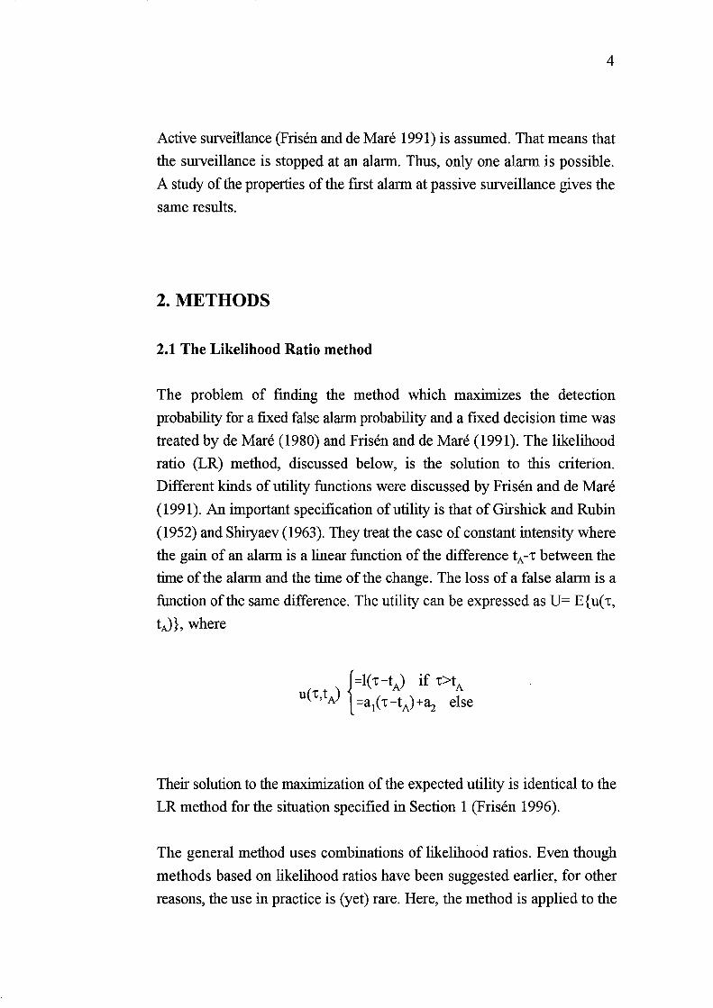
Different kinds of utility functions were discussed by Frisen and de Mare

(1991). An important speciftcation of utility is that of Girshick and Rubin

(1952) and Shiryaev (1963). They treat the case of constant intensity where

the gain of an alarm is a linear function of the difference tA -T between the

time of the alarm and the time of the change. The loss of a false alarm is a

function of the same difference. The utility can be expressed as U= E{u(T,

tJ}, where

Their solution to the maximization of the expected utility is identical to the

LR method for the situation specifted in Section 1 (Frisen 1996).

The general method uses combinations of likelihood ratios. Even though

methods based on likelihood ratios have been suggested earlier, for other

reasons, the use in practice is (yet) rare. Here, the method is applied to the

5

shift case specified in Section 1. The II catastrophe II to be detected at

decision time s is C = { 't ~ s} and the alternative is D = { 't > s}.

The LR method has an alarm set consisting of those ~ for which the

likelihood ratio exceeds a limit:

00

= L w(t)L(t) > K(s) t=1

where wet) = Pr('t=t)/Pr('r~s) and L(t) is the likelihood ratio when 't=t.

For the case of normal distribution, C( s)= { 't ~ s} and D( s )= { 't>s} specified

in Section 1 we have

where

and

h(s) = exp( -(s+ 1)(/11)2/2) Pr('t~s)

which is a nonlinear function of the observations.

In order to achieve the optimal error probabilities discussed by Frisen and

de Mare (1991) an alarm should be given as soon as p(Xg) > K(s).

In order also to achieve maximization of the utility of Shiryaev it is required

that

p(xs» Pr( -r>s) K Pr(-r~s) l-K

where K is a constant. Now we must also consider the function h(s).

2.2 Roberts method

6

Roberts (1966) suggested that an alarm is triggered at the ftrst time s, for

which

s

L L(t) > K t=l

where K is a constant.

This is the limit of the LR method

s

L w(t)L(t) > K(s) t=1

when v tends to zero since both the weights w(t) and the limit K(s) tend to

constants. Thus the Roberts method approximately satisftes the optimality

criterion of Shiryaev (1963) for small values of the intensity v. Roberts

(1966) motivated the method by the conjecture that the intensity parameter

v has very little influence on the LR method, when v is in the interval zero

to 0.2 and thus the weights which depend on v can be omitted. The Roberts

method is sometimes called the Shiryaev-Roberts method. Pollak (1985)

demonstrated that the Roberts procedure is asymptotically (as K -. 00)

minimax. Mevorach and Pollak (1991) examined the expected delay (see

below) by simulations in a small sample setting and concluded that the

difference between this method and the CUSUM method is small.

7

2.3 CUSUM

The cumulative sum

(

C(= L (X(i)-~o) i= 1

is used in several CUSUM- variants. The most commonly advocated variant

gives an alann for the fIrst t for which Ct-Ct-i > h + ki (for some i=I,2, ... t),

where Co=O and hand k are chosen constants (Page 1954).

Sometimes the CUSUM test is defIned in a more general way by likelihood

ratios (Siegmund 1985 and Park and Kim 1990). This reduces to the method

above in the case specifIed in Section 1.

In the simulation study below the slope (~O+~l)/2 is used. The values ~o=O

and ~1=1 gives the slope k=1I2. The requirement of ARLo=l1 gives the

parameter h=0.985. The short ARLO was chosen to make the computer

time, necessary for the study, reasonable.

2.4 The Shew hart method

Shewhart (1931) suggested that an alarm is triggered as soon as a value

which deviates too much from the target is observed. Frisen and de Mare

(1991) demonstrated that this is the same as the LR method with C={ T=S}.

That is p(Xg)=LR(s). For the normal case described in Section 1 this reduces

to p(xs)=x(s). The limit G for an alarm is calculated by the relation:

Pr(X(s»GI~=~O)=lIARLo. ARLo=l1 gives G= 1.3353.

3. RESULTS

F or the Shewhart method exact calculations were made. For the other

methods simulations of 10 000 000 replicates were made for each point in

the diagrams.

8

3.1 Probability of a false alarm

In all simulations the parameters of the different methods were chosen so

that ARLo was equal for all methods (equal to 11) to make them

comparable. To fix the value of ARLo is not the only way to do this, but it

is in accordance with most comparative studies in this area.

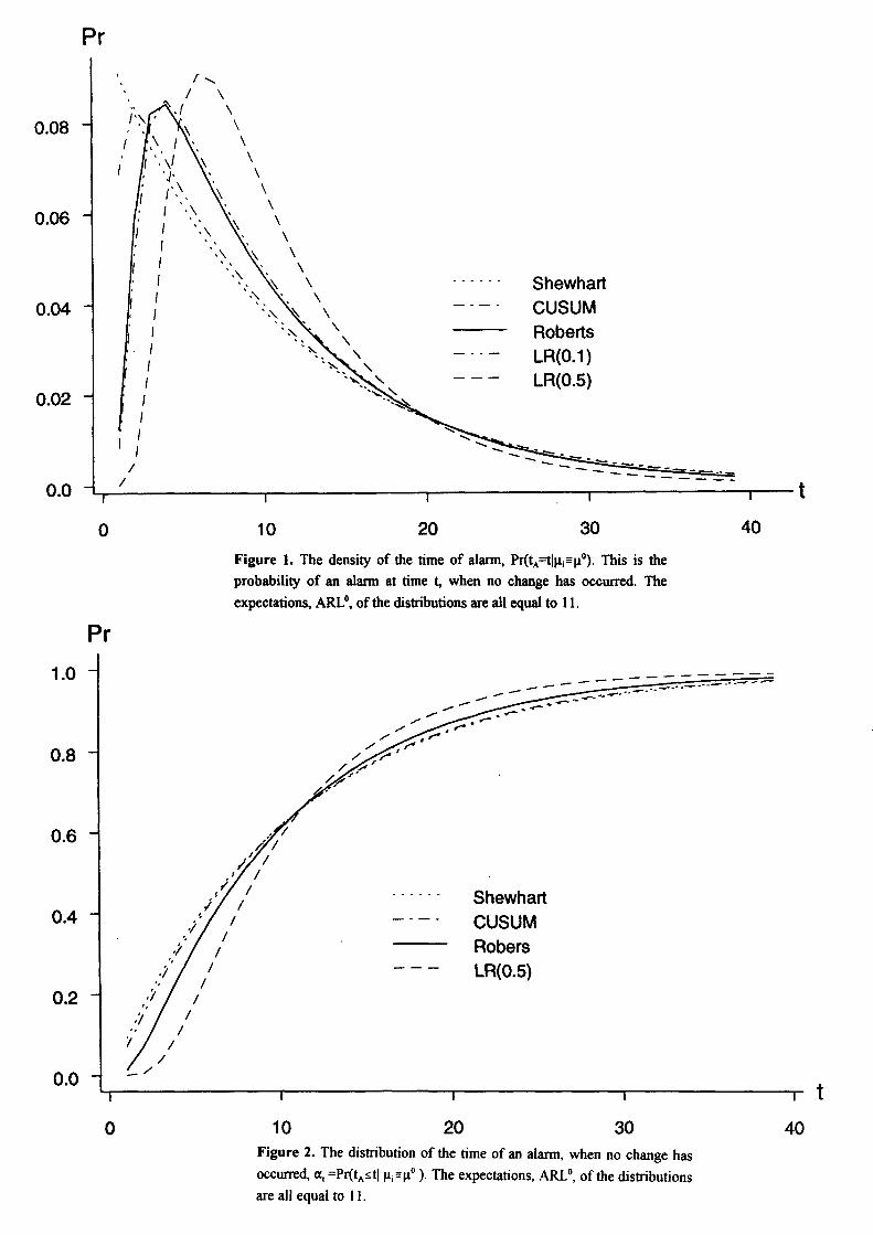
Equal values of ARLo do not imply that the run length distributions are

identical when ~=~o. The distributions can have different shapes. This is

demonstrated in Figures 1 and 2. In Figure 1 the probabilities of an alarm

at a specific time point, when no change has occurred, are given for some

different methods. The skewness of the distributions is less pronounced for

the LR method with a great intensity parameter. For the chosen parameters,

the distributions for the Shewhart and the CUSUM methods are very similar

except at the first point. In Figure 2, the probability of an alarm no later than

at t given that no change has occurred, at = Pre t A ~ t I ~ F ~ 0), is

illustrated. This is also the cumulative distribution ftmction of the run length

when the process is in control. The results of the LR method with

parameters v=O.OOI and v=O.OI, cannot be distinguished from those of the

Roberts method in the scale of the figures and are therefore not included.

The results for v=O.1 are also very close to those of Roberts method and are

included only in Figure 1 where more details can be seen.

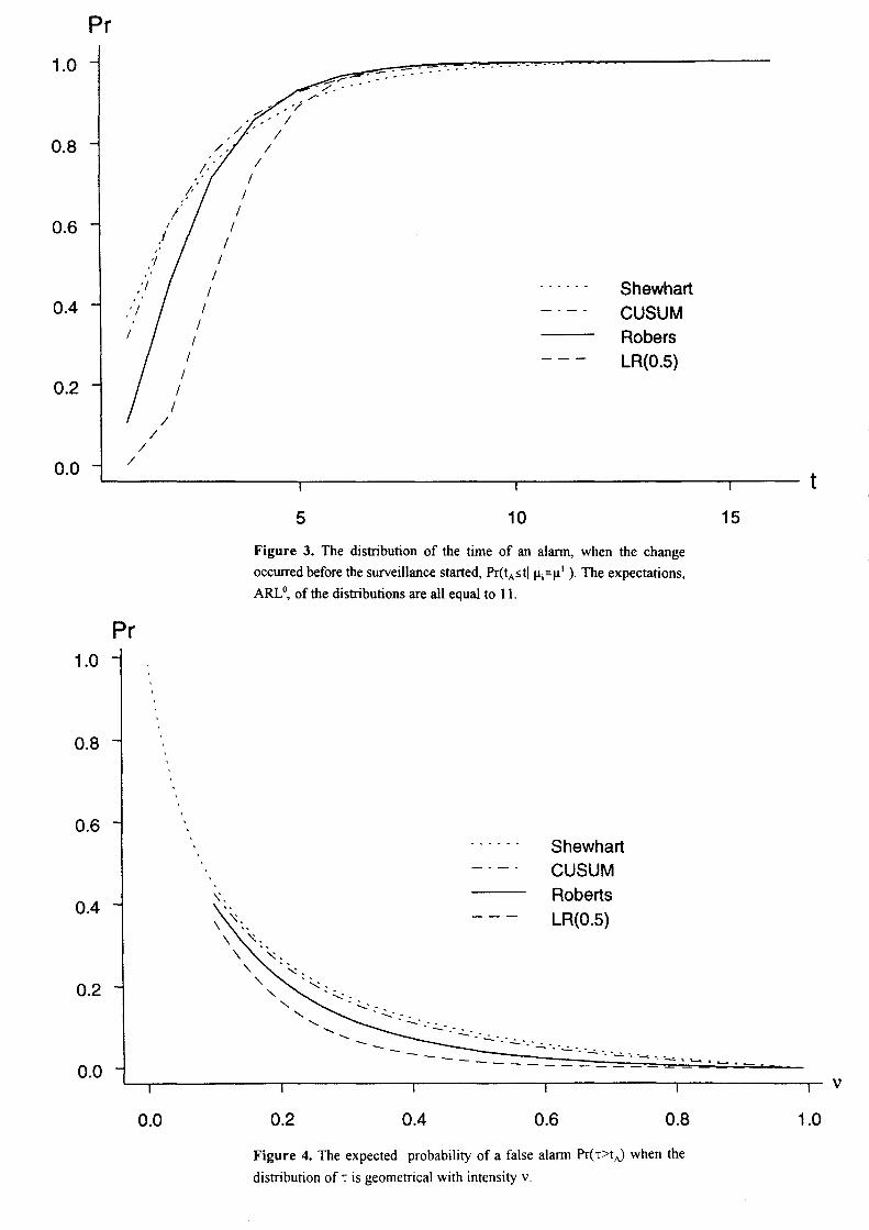
A summarizing measure of the false alarm distribution is the probability of

a false alarm, when the probability of a change has a geometric distribution

with the intensity v. Pr(tA<-r) is illustrated as a function ofv in Figure 4.

00

Pr(tA <-r) = L Pre -r =t)Pr(tA <tl-r =t) t=1

e first factor in the sum does not depend on the method but only on the true

intensity v. The second factor depends only on the run length distribution

when ~=~o. Since the values of the ARLo are equal for all methods only the

different shapes and not their locations will influence the false alarm

probability. Thus only the very modest differences as are seen in Figure 4

can be expected.

9

3.2 Delay of an alarm

As was seen above, the correspondence to the level of significance in an

ordinary test is not a value but a distribution. For the power the

correspondence is still more complicated. To describe the ability of

detecting a change we need a set of run length distributions. Some kind of

summarizing measure is of value.

The distribution of tA , the time of an alarm, when the change occurred

before the surveillance started (-r=I) , that is /l=/lo, is illustrated in Figure

3 for some methods.

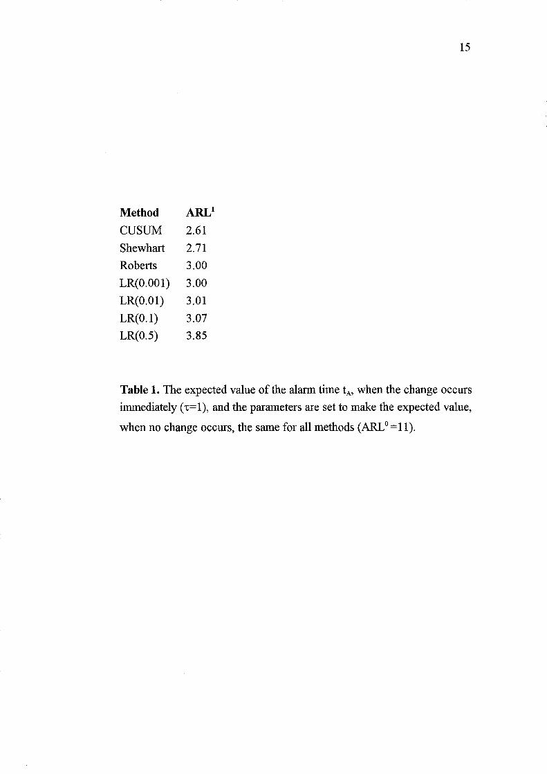
The average run length under the alternative hypothesis, ARL 1, is the mean

number of decisions that must be taken to detect a true level change (that

occurred at the same time as the inspection started). The part of the

definition in the parenthesis is seldom spelled out but seems to be generally

used in the literature on quality control. The values of ARL 1 for the methods

and situations examined are given in Table 1.

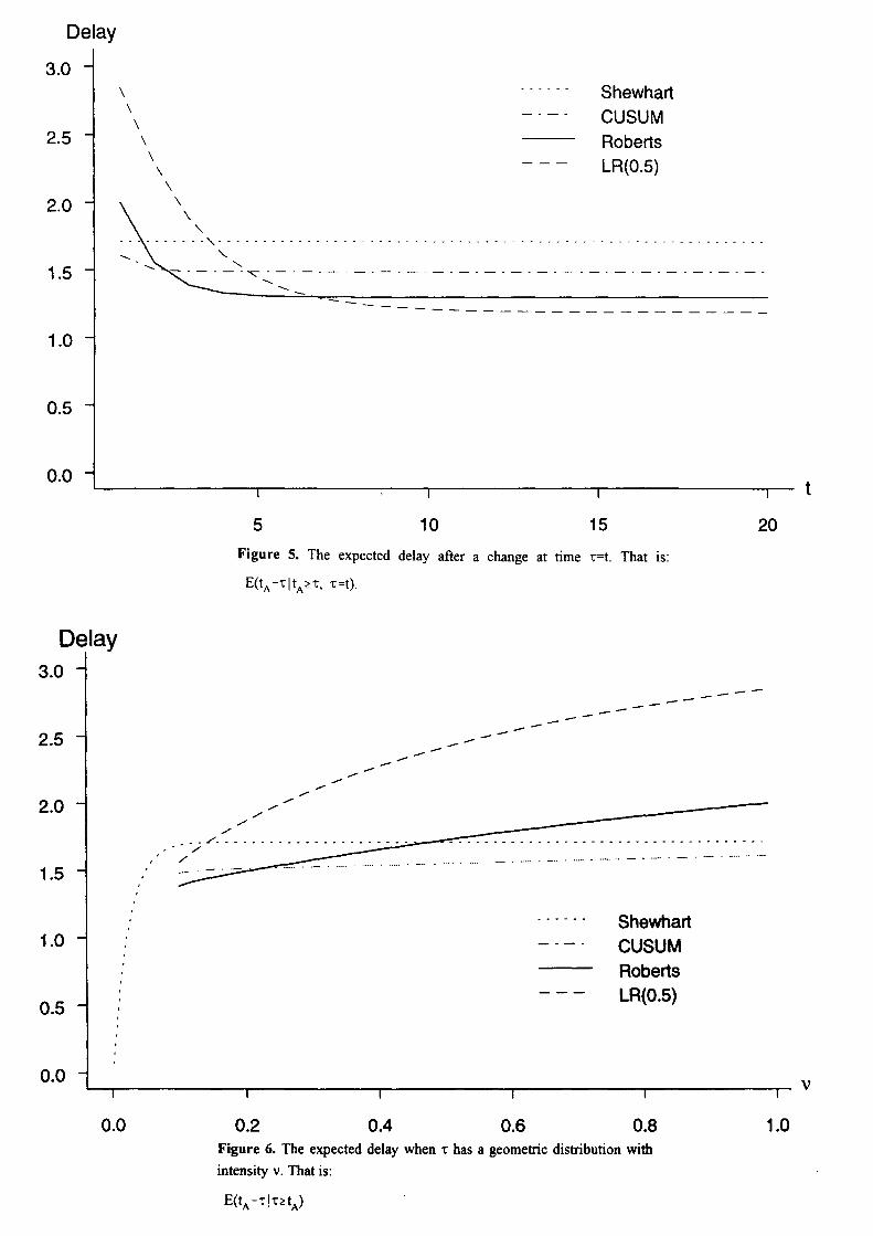
Since the case -r= 1 of is not the only case of interest the expected delay is

calculated also for other values -r=t.

is given in Figure 5. For -r=1 the values of this function equal the values of

ARL 1 - 1. The differences in shapes of these curves demonstrate the need

for other measures than the conventional ARL. Although the Roberts

method has worse ARLl, and thus worse delay for a change at -r=I, than the

Shewhart method, it is better for all other times of change. The CUSUM and

the Shewhart methods are very much alike for -r= 1 but the CUSUM is here

much better for other change points.

In some applications the loss of a delay is directly proportional to the

expected value of the delay. The expected delay also with the respect to the

distribution of -r is:

10

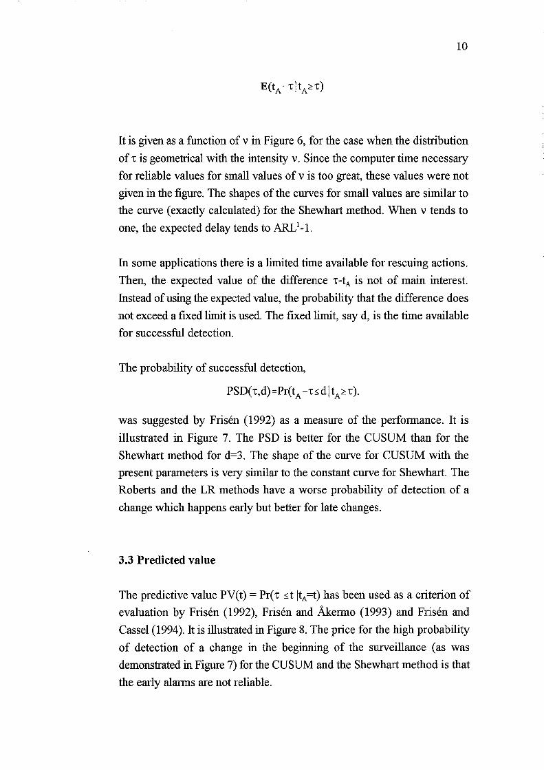
It is given as a function of v in Figure 6, for the case when the distribution

of't" is geometrical with the intensity v. Since the computer time necessary

for reliable values for small values of v is too great, these values were not

given in the figure. The shapes of the curves for small values are similar to

the curve (exactly calculated) for the Shewhart method. When v tends to

one, the expected delay tends to ARL 1_1.

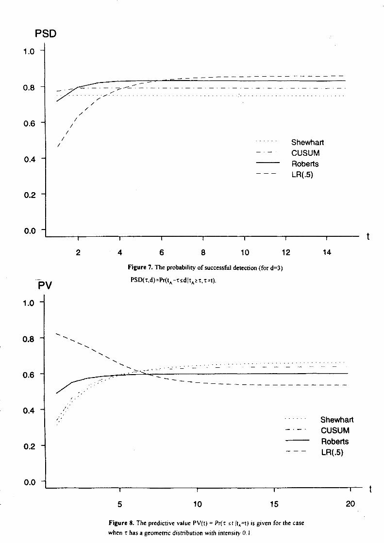
In some applications there is a limited time available for rescuing actions.

Then, the expected value of the difference 't"-tA is not of main interest.

Instead of using the expected value, the probability that the difference does

not exceed a fixed limit is used. The fixed limit, say d, is the time available

for successful detection.

The probability of successful detection,

PSD('t",d)=Pr(tA -'t"~dltA~'t")·

was suggested by Frisen (1992) as a measure of the performance. It is

illustrated in Figure 7. The PSD is better for the CUSUM than for the

Shewhart method for d=3. The shape of the curve for CUSUM with the

present parameters is very similar to the constant curve for Shewhart. The

Roberts and the LR methods have a worse probability of detection of a

change which happens early but better for late changes.

3.3 Predicted value

The predictive value PV(t) = Pr('t" ~t ItA=t) has been used as a criterion of

evaluation by Frisen (1992), Frisen and Akermo (1993) and Frisen and

Cassel (1994). It is illustrated in Figure 8. The price for the high probability

of detection of a change in the beginning of the surveillance (as was

demonstrated in Figure 7) for the CUSUM and the Shewhart method is that

the early alarms are not reliable.

11

4. CONCLUDING REMARKS

At large, the properties differ between the LR methods on one hand and the

Shewhart and the CUSUM methods on the other, in the simulations. In

comparison with this, the choice of the intensity parameter of the LR

method has very little influence on the performance. The results here

confirm the conjecture by Roberts (1966) about the robustness of the LR

method.

That the Roberts method is the limit of the LR method when the intensity

v tends to zero is also seen by the simulated results. The smaller the

intensity parameter, the smaller the difference between the LR method and

the Roberts method. Simulations were made also for v=O.OOI and v=O.OI

but these results were not included in the figures since the differences to

those of the Roberts method are less than the line width. The results for

v=O.1 were included only in the first figure where more details are given.

The Roberts method is a good approximation of the optimal LR method

and thus approximately optimal, for small values of v.

Sometimes the LR method is considered to be a Bayesian method while the

Roberts method is considered a frequentistic one. Here, however all

evaluations are made in the frequentistic framework. No Bayesian

assumptions are necessary for the LR method. The properties of the method

will be better if the intensity parameter is not far from the actual intensity.

However, since the LR method is very robust for misspecification of the

value of the intensity parameter v the gain with a precise search for the best

value of the intensity parameter might not be worthwhile for a specific

application.

The optimal method when the intensity is great should intuitively increase

the probability of early alarms. Some of the present results might seem

surprising in this light and will now be discussed.

The shapes (see Figures 1-3) of the distributions of the alarm time tA might

seem surprising. The probability of a very early alarm by the LR method

12

with a low intensity parameter is greater than for a large value of the

parameter. However, for a low intensity the probability of a late change is

great and thus a thick tail of the distribution of tA is appropriate. As the

expected value ARLo is fixed the only possibility is a high probability in the

beginning. This also causes the differences in false alann probabilities in

Figure 4.

The greater expected delay (see Figures 5 and 6) for the LR method with a

great intensity parameter v might seem surprising. For a fixed false alann

loss I the delay will be less for greater values of the intensity parameter v.

However, now we have a fixed ARLO, and thus a greater value of 1, which

implies that the delay is increased to make the locations of the distributions

of tA equal. The only difference between the distributions is the shape and

this difference causes the expected delay to be greater for the greater values

of the intensity parameter.

The result by Mevorach and Pollak (1991), that the expected delay is

similar for the Robert and CUSUM methods, was not confmned. They

studied an artificial quasi-stationary situation where the time of change, 't,

does not have any influence. For a more realistic situation and the low ARLo

used here the CUSUM in many aspects is very similar to the Shewhart

method and not to the Roberts method.

Figure 7 demonstrates that the Roberts method has higher probability of a

quick (within three time units) detection than the Shewhart method, unless

the change occurs very early. For the LR(O.5) method this difference to the

Shewhart method is still more pronounced.

In Figure 8 the predicted value of an alann is given. This reflects the trust

you should have in an alann. The Roberts method has a relatively constant

predicted value. This means that the same kind of action is appropriate both

for early and late alanns.

13

REFERENCES

Frisen, M. (1992), Evaluations of methods for statistical surveillance,

Statistics in Medicine, 11, 1489-1502.

Frisen M. (1994a) Statistical Surveillance of Business Cycles. Research

report, 1994: 1, Department of Statistics, Goteborg University.

Frisen M. (1994b) A classified bibliography on statistical surveillance.

Research report, 1994, Department of Statistics, Goteborg University.

Frisen M. (1996) Characterization of methods for surveillance by

optimality. Manuscript.

Frisen M. and Cassel C. (1994) Visual evaluations of statistical

surveillance. Research report, 1994:3, Department of Statistics, GOteborg

University.

Frisen, M. and de Mare, 1. (1991), Optimal surveillance, Biometrika, 78,

271-280.

Frisen, M. and Akermo, G. (1993), Comparison between two methods of

surveillance: exponentially weighted moving average vs CUSUM, Research

report, 1993: 1, Department of Statistics, Goteborg University.

Girshick, M. A. and Rubin, H. (1952), A Bayes approach to a quality

control model, Ann. Math. Statist., 23, 114-125.

Mare, J. de (1980), Optimal prediction of catastrophes with application to

Gaussian processes, Ann. Prob. 8, 841-850.

Mevorach, Y. and Pollak, M. (1991), A small sample size comparison of the

CUSUM and Shiryaev-Roberts approaches to changepoint detection,

American 1. o/Mathematical and Management Sciences, 11, 277-298.

Page, E. S. (1954), Continuous inspection schemes, Biometrika, 41,

100-114.

14

Park, C. S. and Kim, B. C. (1990) A CUSUM chart based on log probability

ratio statistic, J. Korean Statistical Society, 19, 160-170.

Pollak, M. (1985) Optimal stopping times for detecting changes III

distributions. Ann. Statist. 13, 206-227.

Roberts S. W. (1966) A comparison of some control chart procedures.

Technometrics, 8,411-30.

Shewhart, W. A. (1931) Economic Control of Quality Control. Reinhold

Company, Princeton N.J.

Shiryaev, A. N. (1963), On optimum methods in quickest detection

problems, Theory Probab. Appl., 8, 22-46.

Siegmund, D. (1985), Sequential analysis. Tests and confidence intervals,

Springer.

Srivastava, M.S. and Wu, Y (1993) Comparison ofEWMA, CUSUM and

Shiryaev-Roberts procedures for detecting a shift in the mean. Ann. Statist.,

21, 645-670.

Wetherill, G.B. and Brown, D.W. (1990), Statistical process control,

London: Chapman and Hall.

Wessman, P. (1996) Some principles for surveillance adopted for

multivariate processes with a common change point. Research report,

1996:2, Department of Statistics, Goteborg University.

Zacks, S. (1983) Survey of classical and Bayesian approaches to the

change-point problem: Fixed sample and sequential procedures of testing

and estimation. in Recent advances in statistics, 245-269.

DEPARTMENT OF STATISTICS

GOTEBORG UNIVERSITY

S-41180 GOTEBORG

SWEDEN

15

Method ARLl

CUSUM 2.61

Shewhart 2.71

Roberts 3.00

LR(O.OOI) 3.00

LR(O.OI) 3.01

LR(O.I) 3.07

LR(0.5) 3.85

Table 1. The expected value of the alarm time tN when the change occurs

immediately (1:= 1), and the parameters are set to make the expected value,

when no change occurs, the same for all methods (ARLo = 11).

0.08

0.06

0.04

0.02

0.0

1.0

0.8

0.6

0.4

0.2

0.0

Pr

f,

'\ ~

'\ ~ , ,

'\ - - - - -- Shewhart " ~

-.-- CUSUM Roberts

---- LR(0.1) --- LR(0.5)

.~.-

--... - - -----------------~~--------~----------~----------._--------_.---t

o

Pr

/ /

/ /

/ _/

o

10 20 30

Figure 1. The density of the time of alann, Pr(tA=tIJ1i= J10). This is the

probability of an alann at time t. when no change has occurred. The

expectations, ARLo, of the distributions are all equal to 11.

~(,;"/ , /

./ / / /

----

; / Shewhart

CUSUM Robers LR(0.5) /

/

/

/ /

10 20 30 Figure 2. The distribution of the time of an alann, when no change has

occurred, at =Pr(tAstl J1i=J1o ). The expectations, ARLO, of the distributions

are all equal to II.

40

-----

40

t

Pr

1.0

0.8

0.6

0.4

0.2

0.0

1.0

0.8

0.6

0.4

0.2

0.0

/ "

:/ :/ /

/

Pr

/ /

/

0.0

"../" ,/", r'

~ ,,'/ , " /

,/,' / /, /

/ /

/

! /

/ /

/ /

/ /

/ /

/ /

/ /

5 10

Shewhart CUSUM Robers

LR(0.5)

Figure 3. The distribution of the time of an alann, when the change

occurred before the surveillance started, Pr(tA:>tl J.li=J.l1 ). The expectations,

ARLO, of the distributions are all equal to 11.

,\,

Shewhart CUSUM Roberts

LR(0.5) "

\ ~,

" \ ~,

\ "

'\ '\

" " " "

.. :...... .... .. .:..... ....

.. ..:.... ...... ~ ...... --=-...... .. _ .... -

15

- - ~~'~-~~-~-~~-~-~~~~'-". ~'-

0.2 0.4 0.6 0.8

Figure 4. The expected probability of a false alann Pr(1'>tJ when the

distribution of" is geometrical with intensity v.

t

v

1.0

Delay

3.0

2.5

2.0

\ \ \

\ \

\ \

\ \ ,

Shewhart CUSUM Roberts LR(0.5)

- - - - - - - - - -,- - - - - - - - - - - - - - - - - - - - - - - - - - - - - - - - - - - - - - - - - - - - - - - - - - - - - - - - - - - - --

1.5

1.0

0.5

0.0

Delay 3.0

2.5

2.0

1.5

1.0

0.5

0.0

0.0

'-"-

------~---------------------------------------......

----------------------

5 10 15 20

Figure 5. The expected delay after a change at time 't=t. That is:

E(tA -'tltAH, 't=t).

-- -- -- --- ---

--------...-

,/ •• __ ,; /. ____________________ ~ _____ -o_. _________________________________ •

,/ - .......... - - ..... . - ....... -

- - .. - - Shewhart ---- CUSUM

Roberts --- LR(0.5)

0.2 0.4 0.6 0.8 Figure 6. The expected delay when 't has a geometric distribution with

intensity v. That is:

1.0

t

v

PSD

1.0

0.8

0.6

0.4

0.2

0.0

. _.

PV

1.0

0.8

- - -- ----------------

~ -:-:. -:-.. ~.'. ~;.-:.~ ~o~~ ... ~ ... ~.o.~ .'.~.'.~.'.~.'.~: .~: ~::~.:~.·.~.·o~.·. ~.'. ~o·.~o·.~.oo~oo

I /

I

......

/ /

I I

2

...... ...... ......

/ .

4 6 8 10 12

Figure 7. The probability of successful detection (for d=3)

PSD(,'C,d)=Pr(tA -"CSdltA~t, t=t) .

...... - . - - . . . . - .. ........ .......... .. ..• ~ ~

t ~ ~ •• - > < - . - -

Shewhart CUSUM Roberts LR(.5)

14

0.6 ~J:O:' .': . --------------------

, . '. 0.4 ,'.

, .

0.2

0.0

5 10 15

Figure 8. The predictive value PV(t) = Pr(t ~t /tA=t) is given for the case

when t has a geometric distribution with intensity 0 J.

Shewhart CUSUM Roberts LR(.5)

20

t

1

Research Report

1994:1 Frisen,M Statistical surveillance of business cycles.

1994:2 Frisen, M Characterization of methods for surveillance by optimality.

1994:3 Frisen, M & Visual evaluations of statistical surveillance. Cassel, C

1994:4 Ekman,C A comparison of two designs for estimating a second order surface with a known maximum.

1994:5 Palaszewski, B Comparing power and multiple significance level for step up and step down multiple test procedures for correlated estimates.

1994:6 Akermo,G Constant predictive value of an alarm.

1994:7 Akermo,G On performance of methods for statistical surveillance.

1994:8 Palaszewksi, B An abstract bootstrap based step down test procedure for testing correlated coefficients in linear models.

1994:9 Ekman,C Saturated designs for second order models.

1994:10 Ekman,C A note on rotatability.

1995:1 Arnkelsdottir, H Surveillance of rare events. On evaluations of the sets method.

1995:2 Svereus, A Detection of gradual changes. Statistical methods in post marketing surveillance.

1995:3 Ekman,C On second order surfaces estimation and rotatability.

1996:1 Ekman, A Sequential analysis of simple hypotheses when using play-the-winner allocation.

1996:2 Wessman,P Some principles for surveillance adopted for multivariate processes with a common change point

1996:3 Frisen, M. & Evaluations of likelihood ratio methods for Wessman, P surveillance.