Conducting Ecological Risk Assessments at Remediation Sites in ...
EPA/600/R-03/040 September 2000
Final Draft
Research Report:
Conducting a Risk Assessmentof Mixtures of Disinfection By-products
(DBPs) for Drinking Water TreatmentSystems
by
Richard C. Hertzberg, John C. Lipscomb, Patricia A. Murphy, Glenn E. Rice and Linda K. Teuschler (Project Lead)
National Center for Environmental AssessmentCincinnati, OH 45268
National Center for Environmental AssessmentOffice of Research and Development
U.S. Environmental Protection AgencyCincinnati, OH 45268

NOTICE
The U.S. Environmental Protection Agency through its Office of Research and Development funded and managed the research described here. It has been subjected to the Agency’s peer and administrative review and has been approved for publication as an EPA document. Mention of trade names or commercial products does not constitute endorsement or recommendation for use.
ii
FOREWORD
This report was developed by the U.S. Environmental Protection Agency's (EPA) Office of Research and Development (ORD), National Center for Environmental Assessment - Cincinnati Office (NCEA-Cin). It contains information concerning the conduct of risk assessments for mixtures of disinfection by-products (DBPs) across various drinking water treatment systems. Under 42 USC § 300 of the Safe Drinking Water Act Amendments of 1996, it is stated that the Agency will “develop new approaches to the study of complex mixtures, such as mixtures found in drinking water...” In addition, the EPA’s Office of Water drafted a Research Plan for Microbial Pathogens and DBPs in Drinking Water that calls for the characterization of DBP mixtures risk (U.S. EPA, 1997a). This report reflects the current results relative to research in this area over the past five years. The report as a whole presents an illustrative DBP mixtures risk characterization; the summary of an expert scientific workshop on this subject; EPA conclusions and recommendations subsequent to the workshop; a conceptual cumulative risk approach; and ideas on future research needs.
This effort has resulted in the production of four reports contained in this document. Appendix I contains an initial report generated as a pre-meeting report to an April 1999 workshop on this subject. It is entitled, Workshop Pre-meeting Report: The Risk Assessment of Mixtures of Disinfection By-Products (DBPs) for Drinking Water Treatment Systems (U.S. EPA, 1999a) and was developed to detail the response addition approach to estimating DBP mixture risk that has recently been developed by NCEA-Cin. Having performed this initial assessment, NCEA-Cin scientists recognized a number of areas for improvement and held a workshop in April 1999 to examine the current method, present ideas to advance the approach, and come to some conclusions relative to new research and development directions. The resulting workshop report is presented as Report 2, entitled, Workshop Report: The Risk Assessment of Mixtures of Disinfection By-Products (DBPs) for Drinking Water Treatment Systems. Finally, EPA scientists have used the information developed in the April 1999 workshop to develop a number of conclusions and recommendations relative to this area of research and to develop a conceptual approach to performing a cumulative risk assessment. This information is presented as Report 1, entitled, EPA Conclusions and Conceptual Approach for Conducting a Risk Assessment of Mixtures of Disinfection By-Products (DBPs) for Drinking Water Treatment Systems.
An external review of this document was conducted June 21-22, 2000, with the primary goal of evaluating Report 1 on EPA’s conclusions and conceptual approach. These reviewers were also invited to comment on the data, methods and discussions presented in Reports 1 and 2 or to add new information and perspectives to this document where needed. A final report containing the summary of the external review comments is contained in Appendix II.
To facilitate the production of this document, work was done under three contractual agreements. The illustrative example of a risk characterization was developed by Dr. Joshua Cohen, under contract #68-C6-0024 with TN & Associates,
iii

Inc. The workshop was conducted on April 26-28, 1999, at EPA’s Andrew W. Breidenbach Environmental Research Center in Cincinnati, Ohio, under contract #68-C7-0011 with SAIC, Inc, who also invited several of the expert scientists who participated. The proceedings of the workshop were then subcontracted to Syracuse Research Corporation and the report prepared by Dr. Pat McGinnis. The independent external review and preparation of comments was conducted under contract #68-C-99-238 with Versar, Inc.
iv
EPA RESEARCHERS
This research on the risk assessment of DBPs was sponsored by U.S. Environmental Protection Agency (EPA), National Center for Environmental Assessment - Cincinnati Division (NCEA-Cin), Comparative Risk Project Team, in collaboration with members of the Cumulative Risk Team and the Risk Assessment Services Team. NCEA-Cin scientists conducted portions of this research, presented at the workshop, and are authors of this report. A number of other EPA scientists also contributed their ideas, provided discussions and review, and wrote text toward completion of this effort. These individuals are listed below.
Primary Authors:
National Center for Environmental Assessment - Cincinnati Division, Cincinnati, OH
Richard C. HertzbergJohn C. LipscombPatricia A. MurphyGlenn E. RiceLinda K. Teuschler (Project Lead)
Contributors:
National Center for Environmental Assessment - Cincinnati Division, Cincinnati, OH
Brenda BoutinRobert BruceMary Beth BrownTerry HarveyChandrika Moudgal
National Center for Environmental Assessment - Immediate Office, Washington, DC
Annie Jarabek Lynn Papa
National Health and Environmental Effects Research Laboratory - Research TrianglePark, NC
Jane Ellen Simmons
National Risk Management Research Laboratory - Cincinnati, OH
Robert Clark Richard Miltner
v
EXTERNAL REVIEW PANEL
This document was subjected to an external review by an expert panel on June 20-21, 2000. A workshop report was generated and finalized in July 2000 (Appendix II). The final draft of this document was greatly influenced and enhanced by the interactions with the expert reviewers. The distinguished members of the expert panel, their affiliations and areas of expertise are:
Mr. Phillipe DanielCamp Dresser and McKeeDrinking water treatment engineering/chemistry
Dr. Lynne HaberToxicology Excellence for Risk AssessmentCarcinogenicity, developmental/reproductive toxicity, mixtures risk assessmentmethodology
Dr. Jay NuckolsColorado State University Exposure modeling, epidemiology, drinking water treatment engineering/chemistry
Dr. Shesh RaiSt. Jude Children’s HospitalStatistical modeling/uncertainty analysis
Dr. Venkat RaoDynCorpCarcinogenicity, developmental/reproductive toxicity, mixtures risk assessmentmethodology
Dr. John ReifColorado State University Epidemiology
Dr. Charles WilkesWilkes Technologies Exposure modeling, statistical modeling/uncertainty analysis
vi

APRIL 1999 WORKSHOP PARTICIPANTS
A workshop was held in April 1999 to examine the response addition approach to DBP mixtures risk assessment, present ideas to change and advance the approach, and generate some conclusions relative to new research and development directions. The distinguished workshop participants included:
Bruce AllenRAS AssociatesChapel Hill, NC
Joshua CohenHarvard Center for Risk AnalysisBoston, MA
Joan ColmanSyracuse Research CorporationSyracuse, NY
Gunther F. CraunStaunton, VA
George M. GrayHarvard Center for Risk AnalysisBoston, MA
Dale HattisClark UniversityWorcester, MA
William HuberQuantitative DecisionsMerion, PA
Mike A. PereiraMedical College of OhioToledo, OH
Charlie PooleUniversity of North CarolinaChapel Hill, NC
William M. StitelerSyracuse Research CorporationSyracuse, NY
Clifford H. WeiselEOHSIPiscataway, NJ
Pat S. FairEPA’s Office of WaterCincinnati, OH
Jennifer McClainRita SchoenyEPA’s Office of WaterWashington, DC
Lynn PapaEPA’s National Center forEnvironmentalAssessment - Immediate OfficeWashington, DC
Brenda BoutinMary Beth BrownRobert M. BruceTerry HarveyRichard C. HertzbergJohn C. LipscombChandrika MoudgalPatricia A. MurphyGlenn E. RiceJeff SwartoutLinda K. TeuschlerEPA’s National Center forEnvironmentalAssessment - Cincinnati Office Cincinnati, OH
vii
DOCUMENT CONTENTS
REPORT 1: EPA Conclusions and Conceptual Approach for Conducting a Risk Assessment of Mixtures of Disinfection By-Products (DBPs) for Drinking Water Treatment Systems. September 30, 2000.
REPORT 2: Workshop Report: Novel Methods for Risk Assessment of Mixtures of Disinfection By-Products (DBPs) for Drinking Water Treatment Systems. January, 2000.
APPENDIX I: Workshop Pre-meeting Report: The Risk Assessment of Mixtures of Disinfection By-Products (DBPs) for Drinking Water Treatment Systems. April, 1999. NCEA-C-0584
APPENDIX II: Peer Review Workshop Report: The Risk Assessment of Mixtures of Disinfection By-Products (DBPs) for Drinking Water Treatment Systems. July, 2000.
viii
REPORT 1:
EPA CONCLUSIONS AND CONCEPTUAL APPROACHFOR CONDUCTING A RISK ASSESSMENT OF MIXTURES OF
DISINFECTION BY-PRODUCTS (DBPs)FOR DRINKING WATER TREATMENT SYSTEMS
September 30, 2000
ix
REPORT 1: TABLE OF CONTENTS
Page
FOREWORD . . . . . . . . . . . . . . . . . . . . . . . . . . . . . . . . . . . . . . . . . . . . . . . . . . . . . . . . iii
EPA RESEARCHERS . . . . . . . . . . . . . . . . . . . . . . . . . . . . . . . . . . . . . . . . . . . . . . . . . v
EXTERNAL REVIEW PANEL . . . . . . . . . . . . . . . . . . . . . . . . . . . . . . . . . . . . . . . . . . . . vi
APRIL 1999 WORKSHOP PARTICIPANTS . . . . . . . . . . . . . . . . . . . . . . . . . . . . . . . . vii
DOCUMENT CONTENTS . . . . . . . . . . . . . . . . . . . . . . . . . . . . . . . . . . . . . . . . . . . . . viii
LIST OF TABLES . . . . . . . . . . . . . . . . . . . . . . . . . . . . . . . . . . . . . . . . . . . . . . . . . . . . xiii
LIST OF FIGURES . . . . . . . . . . . . . . . . . . . . . . . . . . . . . . . . . . . . . . . . . . . . . . . . . . . xiv
EXECUTIVE SUMMARY . . . . . . . . . . . . . . . . . . . . . . . . . . . . . . . . . . . . . . . . . . . . . . xv
1. INTRODUCTION . . . . . . . . . . . . . . . . . . . . . . . . . . . . . . . . . . . . . . . . . . . . R1-1
1.1. PURPOSE . . . . . . . . . . . . . . . . . . . . . . . . . . . . . . . . . . . . . . . . . . . . R1-11.2. STRUCTURE OF THE DOCUMENT . . . . . . . . . . . . . . . . . . . . . . . . R1-21.3. BACKGROUND . . . . . . . . . . . . . . . . . . . . . . . . . . . . . . . . . . . . . . . . R1-5
2. SUMMARY: CURRENT STATE OF THE SCIENCE . . . . . . . . . . . . . . . . . . R1-8
2.1. INTRODUCTION . . . . . . . . . . . . . . . . . . . . . . . . . . . . . . . . . . . . . . . . R1-8
2.1.1. Risk Assessment Paradigm for DBP Mixtures . . . . . . . . . . . . R1-9
2.2. MIXTURES RISK ASSESSMENT METHODS . . . . . . . . . . . . . . . . R1-11
2.2.1. Key Concepts . . . . . . . . . . . . . . . . . . . . . . . . . . . . . . . . . . . . R1-122.2.2. Data-Driven Approaches for Assessing Risks Posed by
Chemical Mixtures . . . . . . . . . . . . . . . . . . . . . . . . . . . . . . . . R1-132.2.3. Risk Characterization and Uncertainty . . . . . . . . . . . . . . . . . R1-152.2.4. Applying Mixtures Methods to DBP Mixtures Risk
Estimation . . . . . . . . . . . . . . . . . . . . . . . . . . . . . . . . . . . . . . . R1-23
2.3. DBP EXPOSURES . . . . . . . . . . . . . . . . . . . . . . . . . . . . . . . . . . . . . R1-27
2.3.1. DBP Concentrations . . . . . . . . . . . . . . . . . . . . . . . . . . . . . . . R1-332.3.2 Tap Water Exposure . . . . . . . . . . . . . . . . . . . . . . . . . . . . . . . R1-36
x
REPORT 1: TABLE OF CONTENTS (cont.)
Page
2.4. DBP HEALTH EFFECTS DATA (HAZARD IDENTIFICATIONAND DOSE-RESPONSE) . . . . . . . . . . . . . . . . . . . . . . . . . . . . . . . . R1-38
2.4.1. Summary of Epidemiology Studies . . . . . . . . . . . . . . . . . . . . R1-392.4.2. Summary of Single Chemical Toxicology Studies . . . . . . . . R1-582.4.3. Summary of Mixtures Toxicology In Vivo and In Vitro
Studies . . . . . . . . . . . . . . . . . . . . . . . . . . . . . . . . . . . . . . . . . R1-70
2.5. THE UNIDENTIFIED FRACTION OF DBPS . . . . . . . . . . . . . . . . . . R1-82
2.6. RISK ASSESSMENT USING A RESPONSE ADDITION APPROACH . . . . . . . . . . . . . . . . . . . . . . . . . . . . . . . . . . . . . . . . . . R1-85
2.6.1. Development of Distributions of Risks . . . . . . . . . . . . . . . . . R1-91
3. EPA’S MAIN CONCLUSIONS AND RECOMMENDATIONS BASEDON THE APRIL 1999 WORKSHOP . . . . . . . . . . . . . . . . . . . . . . . . . . . . . R1-105
3.1. EPA RECOMMENDATIONS: INTEGRATION OF EPIDEMIOLOGIC AND TOXICOLOGIC DATA IN THE RISK ASSESSMENT . . . . . . . . . . . . . . . . . . . . . . . . . . . . . . . . . . . . . . . R1-106
3.2. IMPROVEMENTS IN EXPOSURE CHARACTERIZATION . . . . . . R1-109
3.3. ACCOUNTING FOR POTENTIAL TOXICITY OF UNIDENTIFIED DBPs . . . . . . . . . . . . . . . . . . . . . . . . . . . . . . . . . . R1-112
3.4. RISK ASSESSMENT OF DEVELOPMENTAL ANDREPRODUCTIVE EFFECTS . . . . . . . . . . . . . . . . . . . . . . . . . . . . . R1-114
3.5. RISK ASSESSMENT OF CARCINOGENIC EFFECTS . . . . . . . . R1-116
3.6. ACCOUNTING FOR VARIABILITY AND UNCERTAINTY . . . . . . R1-118
3.6.1. Dose-Response Issues . . . . . . . . . . . . . . . . . . . . . . . . . . . R1-1183.6.2. Exposure Issues . . . . . . . . . . . . . . . . . . . . . . . . . . . . . . . . . R1-120
3.7. MIXTURE RISK CHARACTERIZATION METHODS . . . . . . . . . . . R1-121
xi
REPORT 1: TABLE OF CONTENTS (cont.)
Page
4. CONCEPTUAL MODEL FOR A CUMULATIVE RISK APPROACH . . . . . R1-124
4.1. MODEL CONSIDERATIONS AND REQUIREMENTS . . . . . . . . . R1-1244.2. CUMULATIVE RISK APPROACH . . . . . . . . . . . . . . . . . . . . . . . . . R1-126
4.2.1 Relative Potency Factors . . . . . . . . . . . . . . . . . . . . . . . . . . R1-1334.2.2. Cumulative Relative Potency Factors . . . . . . . . . . . . . . . . . R1-1424.2.3. Unidentified DBPs . . . . . . . . . . . . . . . . . . . . . . . . . . . . . . . R1-1474.2.4. Discussion . . . . . . . . . . . . . . . . . . . . . . . . . . . . . . . . . . . . . R1-148
5. RESEARCH NEEDS . . . . . . . . . . . . . . . . . . . . . . . . . . . . . . . . . . . . . . . . R1-150
5.1. METHODS RESEARCH . . . . . . . . . . . . . . . . . . . . . . . . . . . . . . . . R1-150
5.2. RESEARCH ON APPLICATION OF A CUMULATIVERELATIVE POTENCY FACTOR APPROACH . . . . . . . . . . . . . . . R1-151
5.3. EPIDEMIOLOGIC RESEARCH . . . . . . . . . . . . . . . . . . . . . . . . . . . R1-151
5.4. DEVELOPMENT OF TOXICOLOGIC DATA . . . . . . . . . . . . . . . . . R1-152
6. REFERENCES . . . . . . . . . . . . . . . . . . . . . . . . . . . . . . . . . . . . . . . . . . . . R1-155
APPENDIX R1-1: Summary: ILSI Workshop on Unidentified DBPs . . . . . . . . R1-171
xii

LIST OF TABLES
No. Title Page
1 Methods for Component Data . . . . . . . . . . . . . . . . . . . . . . . . . . . . . R1-16
2 Methods for Whole Mixture Data . . . . . . . . . . . . . . . . . . . . . . . . . . . R1-19
3 DBPs Commonly Found in Finished Drinking Water . . . . . . . . . . . . R1-34
4 Summary of Interview-Based, Case-Control and Cohort Studies for Cancer . . . . . . . . . . . . . . . . . . . . . . . . . . . . . . . . . . . . . . . . . . . . R1-41
5 Summary of Epidemiological Studies for Adverse Pregnancy Outcomes . . . . . . . . . . . . . . . . . . . . . . . . . . . . . . . . . . . . . . . . . . . . R1-48
6 Verified DBP Assessments on EPA’s Integrated Risk Information System (IRIS) . . . . . . . . . . . . . . . . . . . . . . . . . . . . . . . . R1-59
7 Available Toxicity Data for DBP Mixtures . . . . . . . . . . . . . . . . . . . . R1-71
8 Identified Disinfection By-Products (Set k) for the Response Addition Illustration . . . . . . . . . . . . . . . . . . . . . . . . . . . . . . . . . . . . . R1-89
9 Tap Water Consumption in the General Population (mL/kg-day) by 5-Year Age Groups . . . . . . . . . . . . . . . . . . . . . . . . . . . . . . . . . . . R1-96
10 DBP Concentrations Used in the Illustration . . . . . . . . . . . . . . . . . . R1-97
11 Incremental Cancer Risk per mg/kg-day for Identified DBPs . . . . . R1-99
12 Hypothetical Characterization of the Toxicologic Properties of Five DBPs that are Liver Carcinogens in Animal Studies . . . . . . . R1-140
13 Hypothetical Example: Relative Potency Factors (RPF) and Equivalent Exposures for Five Liver Carcinogens . . . . . . . . . . . . . R1-141
14 Hypothetical Characterization of Several Relative Potency Factors for the Same DBP Mixture; Different Routes, Different Effects . . . . . . . . . . . . . . . . . . . . . . . . . . . . . . . . . . . . . . . R1-147
xiii
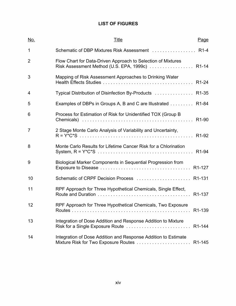
LIST OF FIGURES
No. Title Page
1 Schematic of DBP Mixtures Risk Assessment . . . . . . . . . . . . . . . . . R1-4
2 Flow Chart for Data-Driven Approach to Selection of Mixtures Risk Assessment Method (U.S. EPA, 1999c) . . . . . . . . . . . . . . . . . R1-14
3 Mapping of Risk Assessment Approaches to Drinking Water Health Effects Studies . . . . . . . . . . . . . . . . . . . . . . . . . . . . . . . . . . . R1-24
4 Typical Distribution of Disinfection By-Products . . . . . . . . . . . . . . . R1-35
5 Examples of DBPs in Groups A, B and C are Illustrated . . . . . . . . . R1-84
6 Process for Estimation of Risk for Unidentified TOX (Group B Chemicals) . . . . . . . . . . . . . . . . . . . . . . . . . . . . . . . . . . . . . . . . . . . R1-90
7 2 Stage Monte Carlo Analysis of Variability and Uncertainty, R = Y*C*S . . . . . . . . . . . . . . . . . . . . . . . . . . . . . . . . . . . . . . . . . . . . R1-92
8 Monte Carlo Results for Lifetime Cancer Risk for a Chlorination System, R = Y*C*S . . . . . . . . . . . . . . . . . . . . . . . . . . . . . . . . . . . . . R1-94
9 Biological Marker Components in Sequential Progression from Exposure to Disease . . . . . . . . . . . . . . . . . . . . . . . . . . . . . . . . . . . R1-127
10 Schematic of CRPF Decision Process . . . . . . . . . . . . . . . . . . . . . R1-131
11 RPF Approach for Three Hypothetical Chemicals, Single Effect, Route and Duration . . . . . . . . . . . . . . . . . . . . . . . . . . . . . . . . . . . . R1-137
12 RPF Approach for Three Hypothetical Chemicals, Two Exposure Routes . . . . . . . . . . . . . . . . . . . . . . . . . . . . . . . . . . . . . . . . . . . . . . R1-139
13 Integration of Dose Addition and Response Addition to Mixture Risk for a Single Exposure Route . . . . . . . . . . . . . . . . . . . . . . . . . R1-144
14 Integration of Dose Addition and Response Addition to Estimate Mixture Risk for Two Exposure Routes . . . . . . . . . . . . . . . . . . . . . R1-145
xiv

EXECUTIVE SUMMARY
Human exposure to disinfection by-products (DBPs) in drinking water presents
an example of a multiple chemical, multiple route exposure that is ubiquitous across all
segments of the U.S. population, as well as the populations of many developed
countries around the world. DBPs may be present in liquid, vapor, or aerosol form(s);
can enter the body via ingestion, respiration, or dermal penetration; and may be
metabolized before distribution to the target organ(s).
Disinfectants such as free chlorine, combined chlorine, ozone, and chlorine
dioxide react with naturally occurring organic and inorganic material in the incoming
source water to produce a variety of DBPs. Several hundred chemically distinct DBPs
have been identified in the laboratory, but in general, as illustrated for the organic
halogens in Figure E-1, approximately 50% of the DBPs is typically made up of an
unknown number of unidentified chemicals (Miltner et al., 1990; Richardson, 1998;
Weinberg, 1999).
Exposure to DBPs is a potential human health hazard; both the epidemiologic
and toxicologic literature provide some evidence of potential adverse health effects.
Taken as a whole, epidemiologic studies on chlorinated drinking water offer some
evidence of an association with certain cancers, reproductive and developmental
effects, warranting further investigation. In contrast, in whole mixture studies, toxic
effects have not been observed when animals are exposed to finished drinking water,
but there is evidence of mutagenicity in in vitro studies of drinking water extracts and
concentrates. In in vivo studies at high doses of individual DBPs and some defined
xv

Percentage of Total Organic Halogen Accounted for by Known DBPs (on a Molar Basis)*
Cyanogen
Bromochloro-acetic Acid
Trihalomethanes
Chloride
20.1%
10.0%
2.8%
Haloaceto-nitriles
Chloral Hydrate
Unknown Sum of 5 Organic Halogen Haloacetic Acids
62.4%
*California water, 1997 (raw-water bromide = 0.15 mg/L): Total organic halogen = 172 µg/L
FIGURE E-1
Typical Distribution of Disinfection By-Products
Source: Stuart Krasner, Metropolitan Water District of So. California, 1999
xvi
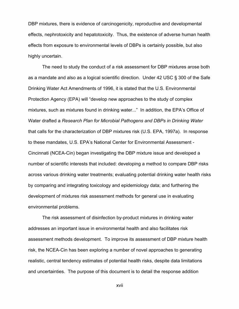
DBP mixtures, there is evidence of carcinogenicity, reproductive and developmental
effects, nephrotoxicity and hepatotoxicity. Thus, the existence of adverse human health
effects from exposure to environmental levels of DBPs is certainly possible, but also
highly uncertain.
The need to study the conduct of a risk assessment for DBP mixtures arose both
as a mandate and also as a logical scientific direction. Under 42 USC § 300 of the Safe
Drinking Water Act Amendments of 1996, it is stated that the U.S. Environmental
Protection Agency (EPA) will “develop new approaches to the study of complex
mixtures, such as mixtures found in drinking water...” In addition, the EPA’s Office of
Water drafted a Research Plan for Microbial Pathogens and DBPs in Drinking Water
that calls for the characterization of DBP mixtures risk (U.S. EPA, 1997a). In response
to these mandates, U.S. EPA’s National Center for Environmental Assessment -
Cincinnati (NCEA-Cin) began investigating the DBP mixture issue and developed a
number of scientific interests that included: developing a method to compare DBP risks
across various drinking water treatments; evaluating potential drinking water health risks
by comparing and integrating toxicology and epidemiology data; and furthering the
development of mixtures risk assessment methods for general use in evaluating
environmental problems.
The risk assessment of disinfection by-product mixtures in drinking water
addresses an important issue in environmental health and also facilitates risk
assessment methods development. To improve its assessment of DBP mixture health
risk, the NCEA-Cin has been exploring a number of novel approaches to generating
realistic, central tendency estimates of potential health risks, despite data limitations
and uncertainties. The purpose of this document is to detail the response addition
xvii
method developed to estimate DBP mixtures risk; discuss the state of DBP toxicity and
exposure data; present available methods for mixtures risk characterization that may be
applicable; explore alternative methodologies; and make recommendations for future
applications and methodological developments. This effort has resulted in the
production of three interrelated research reports and an external review report
contained in this document, as follows:
• Report 1, September, 2000: EPA’s conclusions, recommendations, conceptual approach, and future directions regarding the conduct of a DBP mixture risk assessment. Although new information and ideas not in Report 2 or Appendix I are included, Report 1 is not written as a stand-alone document; it is meant to be read in conjunction with Report 2 and Appendix I.
• Report 2, January, 2000: Summary of presentations and discussions at an April 1999 workshop where scientists examined an illustrative example of a DBP mixtures risk assessment, presented ideas to advance the approach, and recommended research and development directions.
• Appendix I, April, 1999: An illustrative example of a DBP mixtures risk assessment using a response addition approach developed by NCEA-Cin, including data, assumptions and statistical methods used. Shows resulting risk distributions and uncertainty analysis.
• Appendix II, July, 2000: External scientific review comments and recommendations, concentrated primarily on Report 1 of this document.
The authors of this document have chosen to evaluate DBP health effects using
mixture risk assessment approaches, rather than assessing each chemical separately.
These approaches acknowledge real human exposures, as well as account for any
compounded effects from exposure to the low levels of multiple DBPs that are found in
drinking water. Because toxic effects have not been observed in animal studies when
the exposures are to low doses of DBPs and because the epidemiologic data are
inconsistent across studies with only relatively weak to moderate associations noted,
the existence of human health risks is questionable, but cannot be entirely dismissed.
xviii

If it is assumed, however, that the human health effects suggested in some
epidemiologic studies are real, then one hypothesis that explains the discrepancies
between the epidemiologic results and the lack of effects in animals exposed to finished
drinking water (i.e., water that has undergone a disinfection process) is that there is an
effect from exposure to the mixture of DBPs greater than what would be expected from
a low level exposure to any individual DBP. The authors of this document have chosen
this hypothesis — that adverse health effects exist and are attributable to exposure to
the complex mixture — as the basic premise on which to build a risk assessment
approach.
The EPA has both experience and guidance available to address the issue of
DBP mixture risk estimation. The EPA generally follows the paradigm established by
the National Academy of Sciences (NRC, 1983) when performing a human health risk
assessment. This paradigm consists of a group of inter-related processes: hazard
identification, dose response assessment, exposure assessment and risk
characterization. These processes are also the basis for the current DBP mixtures risk
assessment and are the elements that must be addressed in making improvements.
The EPA began to address concerns over health risks from multiple chemical
exposures in the 1980s and issued its Guidelines for the Health Risk Assessment of
Chemical Mixtures in 1986 (U.S. EPA, 1986). Continued interest and research in this
area and in multiple route exposures has resulted in other documents over the years
(U.S. EPA, 1989a,b, 1990, 1999b). In 2001, the EPA is expected to release further
guidance on the assessment of risks posed by exposures to chemical mixtures (U.S.
EPA, 1999c, 2000a).
xix
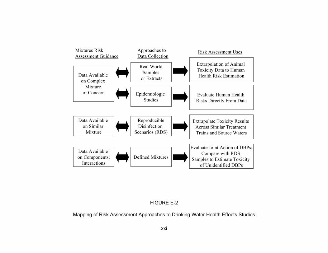
Three basic approaches are available for quantifying health risk for a chemical
mixture, depending on the type of data available to the risk assessor (U.S. EPA, 1986,
1999c, 2000a). These approaches are: data on the complex mixture of concern; data
on a similar mixture; or data on the individual components of the mixture or on their
interactions. Figure E-2 illustrates that these three approaches can be mapped directly
to three toxicity testing scenarios recommended by an International Life Sciences
Institute (ILSI) expert panel on DBP mixtures toxicity (ILSI, 1998). Figure E-2 also
shows the potential uses of such data for risk assessment.
The initial risk assessment was done to illustrate how DBP mixture risk could be
quantified using occurrence data, DBP toxicity estimates, and human drinking water
consumption rate data (U.S. EPA, 1998a, 1999a). (The details of this risk
characterization, including exposure estimates, toxicity values and risk estimates are
presented in full in Appendix I; presentations of this analysis from an April 1999
workshop are summarized in Section 2 of Report 2.)
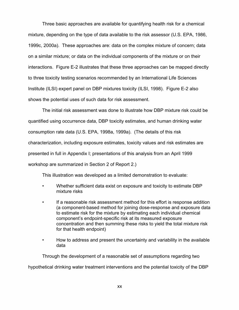
This illustration was developed as a limited demonstration to evaluate:
• Whether sufficient data exist on exposure and toxicity to estimate DBP mixture risks
• If a reasonable risk assessment method for this effort is response addition (a component-based method for joining dose-response and exposure data to estimate risk for the mixture by estimating each individual chemical component’s endpoint-specific risk at its measured exposure concentration and then summing these risks to yield the total mixture risk for that health endpoint)
• How to address and present the uncertainty and variability in the available data
Through the development of a reasonable set of assumptions regarding two
hypothetical drinking water treatment interventions and the potential toxicity of the DBP
xx
Mixtures Risk Assessment Guidance
Data Available on Complex
Mixture of Concern
Data Available on Similar
Mixture
Data Available on Components;
Interactions
Approaches to Data Collection
Real World Samples
or Extracts
Epidemiologic Studies
Reproducible Disinfection
Scenarios (RDS)
Defined Mixtures
FIGURE E-2
Risk Assessment Uses
Extrapolation of Animal Toxicity Data to Human Health Risk Estimation
Evaluate Human Health Risks Directly From Data
Extrapolate Toxicity Results Across Similar Treatment Trains and Source Waters
Evaluate Joint Action of DBPs;Compare with RDS
Samples to Estimate Toxicity of Unidentified DBPs
Mapping of Risk Assessment Approaches to Drinking Water Health Effects Studies
xxi
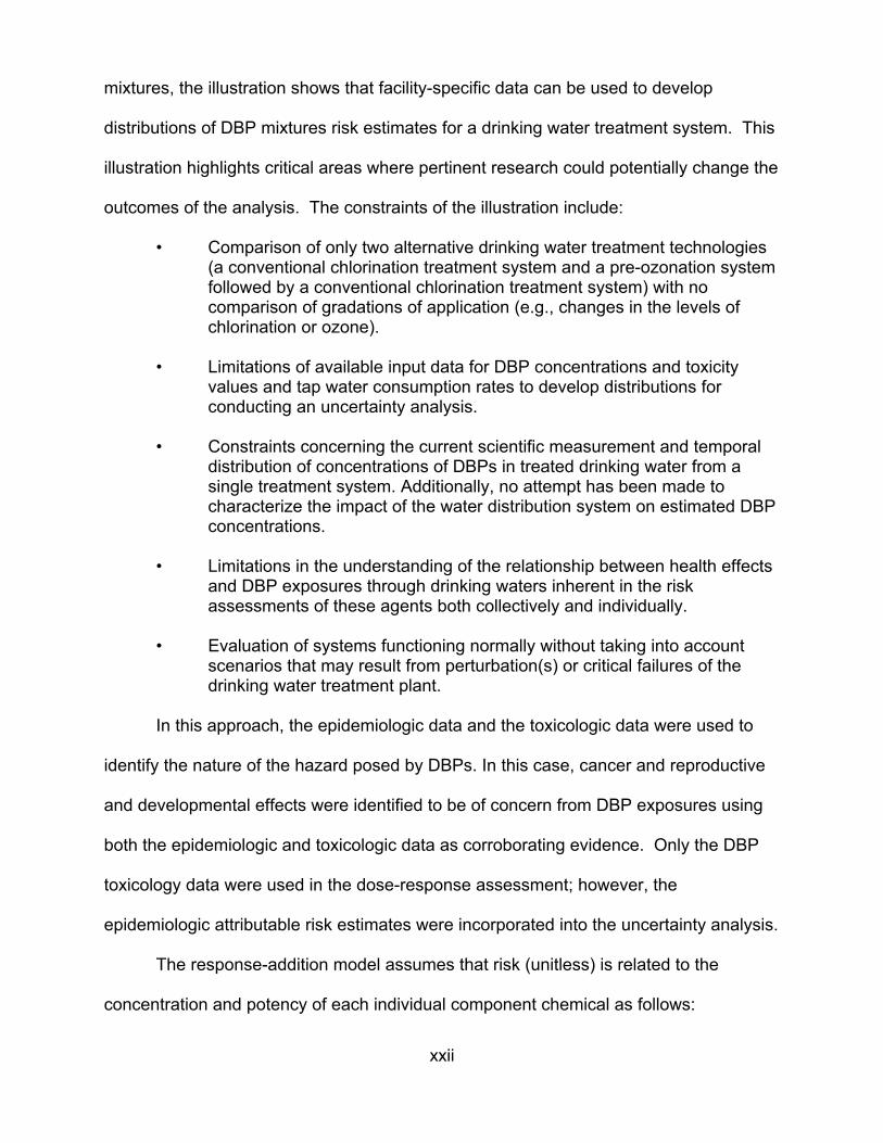
mixtures, the illustration shows that facility-specific data can be used to develop
distributions of DBP mixtures risk estimates for a drinking water treatment system. This
illustration highlights critical areas where pertinent research could potentially change the
outcomes of the analysis. The constraints of the illustration include:
• Comparison of only two alternative drinking water treatment technologies (a conventional chlorination treatment system and a pre-ozonation system followed by a conventional chlorination treatment system) with no comparison of gradations of application (e.g., changes in the levels of chlorination or ozone).
• Limitations of available input data for DBP concentrations and toxicity values and tap water consumption rates to develop distributions for conducting an uncertainty analysis.
• Constraints concerning the current scientific measurement and temporal distribution of concentrations of DBPs in treated drinking water from a single treatment system. Additionally, no attempt has been made to characterize the impact of the water distribution system on estimated DBP concentrations.
• Limitations in the understanding of the relationship between health effects and DBP exposures through drinking waters inherent in the risk assessments of these agents both collectively and individually.
• Evaluation of systems functioning normally without taking into account scenarios that may result from perturbation(s) or critical failures of the drinking water treatment plant.
In this approach, the epidemiologic data and the toxicologic data were used to
identify the nature of the hazard posed by DBPs. In this case, cancer and reproductive
and developmental effects were identified to be of concern from DBP exposures using
both the epidemiologic and toxicologic data as corroborating evidence. Only the DBP
toxicology data were used in the dose-response assessment; however, the
epidemiologic attributable risk estimates were incorporated into the uncertainty analysis.
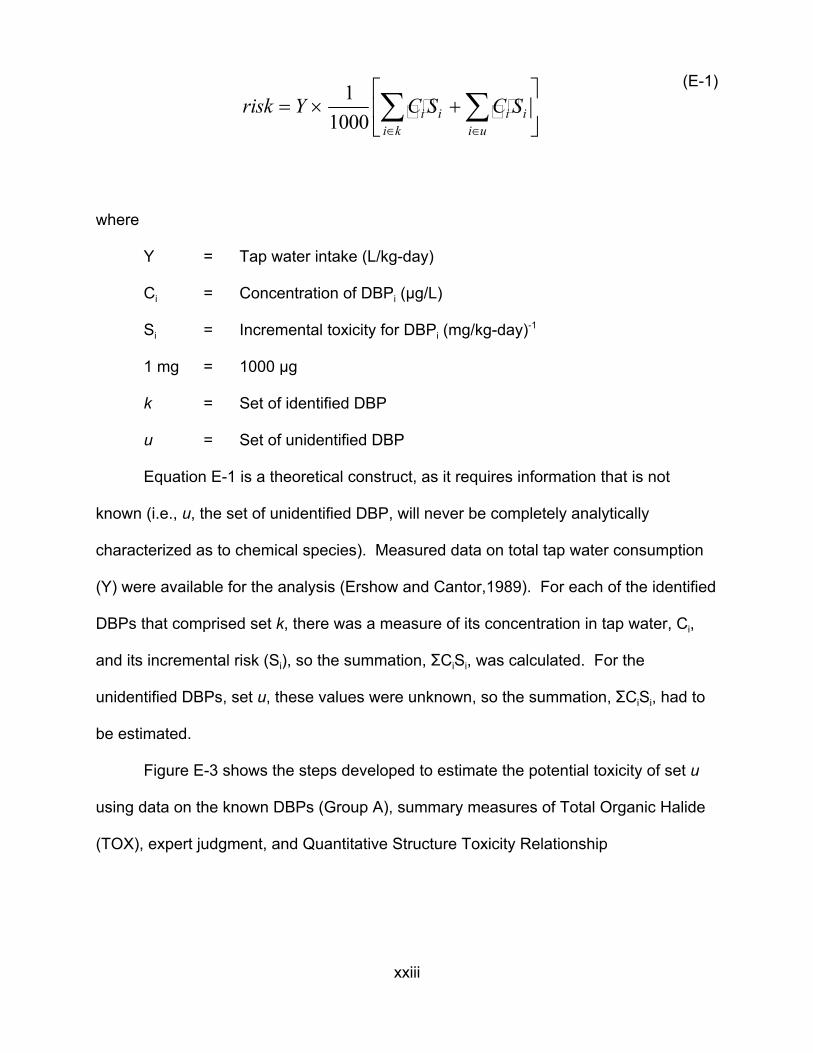
The response-addition model assumes that risk (unitless) is related to the
concentration and potency of each individual component chemical as follows:
xxii
i u∈i k
1 (E-1) risk = × ∑ C S +∑ C SY i i i i 1000 ∈
where
Y = Tap water intake (L/kg-day)
Ci = Concentration of DBPi (µg/L)
Si = Incremental toxicity for DBPi (mg/kg-day)-1
1 mg = 1000 µg
k = Set of identified DBP
u = Set of unidentified DBP
Equation E-1 is a theoretical construct, as it requires information that is not
known (i.e., u, the set of unidentified DBP, will never be completely analytically
characterized as to chemical species). Measured data on total tap water consumption
(Y) were available for the analysis (Ershow and Cantor,1989). For each of the identified
DBPs that comprised set k, there was a measure of its concentration in tap water, Ci,
and its incremental risk (Si), so the summation, GCiSi, was calculated. For the
unidentified DBPs, set u, these values were unknown, so the summation, GCiSi, had to
be estimated.
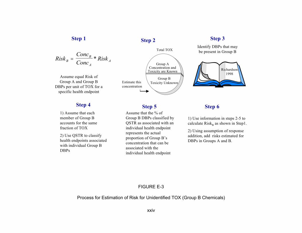
Figure E-3 shows the steps developed to estimate the potential toxicity of set u
using data on the known DBPs (Group A), summary measures of Total Organic Halide
(TOX), expert judgment, and Quantitative Structure Toxicity Relationship
xxiii
A
Assume equal Risk of Group A and Group B
DBPs per unit of TOX for a specific health endpoint
Step 4 1) Assume that each member of Group B accounts for the same fraction of TOX
2) Use QSTR to classify health endpoints associated with individual Group B DBPs
Step 1 Step 2 Step 3 Identify DBPs that may
ConcB
Total TOX be present in Group B
RiskB = Conc
* Risk A
Estimate this concentration
Group AConcentration and
Toxicity are Known
Group B Toxicity Unknown
Step 5 Assume that the % of Group B DBPs classified by QSTR as associated with an individual health endpoint represents the actual proportion of Group B’s concentration that can be associated with the individual health endpoint
FIGURE E-3
Richardson 1998
Step 6
1) Use information in steps 2-5 to calculate RiskB as shown in Step1.
2) Using assumption of response addition, add risks estimated for DBPs in Groups A and B.
Process for Estimation of Risk for Unidentified TOX (Group B Chemicals)
xxiv

(QSTR) modeling techniques. This process estimated risk only for the unidentified
organic halides (Group B); the non-halogenated DBPs (Group C) were not included.
The total endpoint-specific risk, using equation E-1, is the sum of the risks for the
identified DBPs (Group A), as calculated from known toxicity and measurement data,
and the unidentified DBPs (Group B), as estimated using Steps 1 through 6 of Figure
E-3.
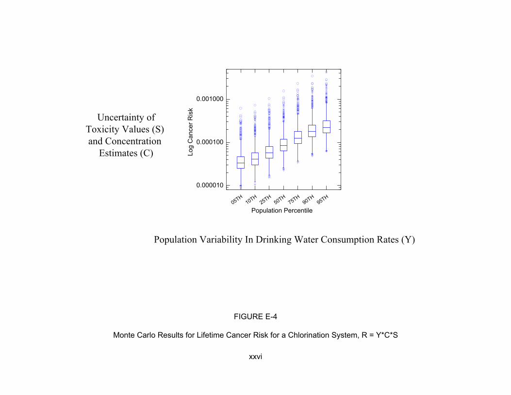
To address variability and uncertainty, a two-stage Monte Carlo analysis was
performed to calculate distributions of DBP mixture risk. Input distributions were
developed to quantify variability (heterogeneity) in the population tap water consumption
rates (Y), (i.e., the range of plausible risks resulting from differences among members of
the population) and to quantify uncertainty (i.e., the range of plausible risks for each
individual corresponding to alternative plausible assumptions) for DBP concentration
data (Ci) and DBP toxicity estimates (Si). The result of such an analysis is the
development of risk distributions, as shown in Figure E-4, that reflect variability on the
X-axis and uncertainty on the Y-axis.
EPA held a workshop in April 1999 to examine the response addition illustration
and to advance the development of methodology to assess health risk for mixtures of
drinking water DBPs. The workshop assembled a multi-disciplinary group of scientists
that worked together to formulate a range of approaches to solving this problem. They
then determined the most practical and scientifically sound directions the EPA should
take to improve the risk assessment (see Charge to Participants, Attendees in Report
2). As a result of the April 1999 workshop, EPA identified the major issues for
consideration regarding improvement of the DBP mixtures risk assessment
xxv
0.001000
Uncertainty of Toxicity Values (S) and Concentration
Estimates (C) Log
Can
cer R
isk
0.000100
0.000010
H1 H
2 H5 H
7 H9 H
9 H50 T T0 T5 T0 T5 T0 T5
Population Percentile
Population Variability In Drinking Water Consumption Rates (Y)
FIGURE E-4
Monte Carlo Results for Lifetime Cancer Risk for a Chlorination System, R = Y*C*S
xxvi
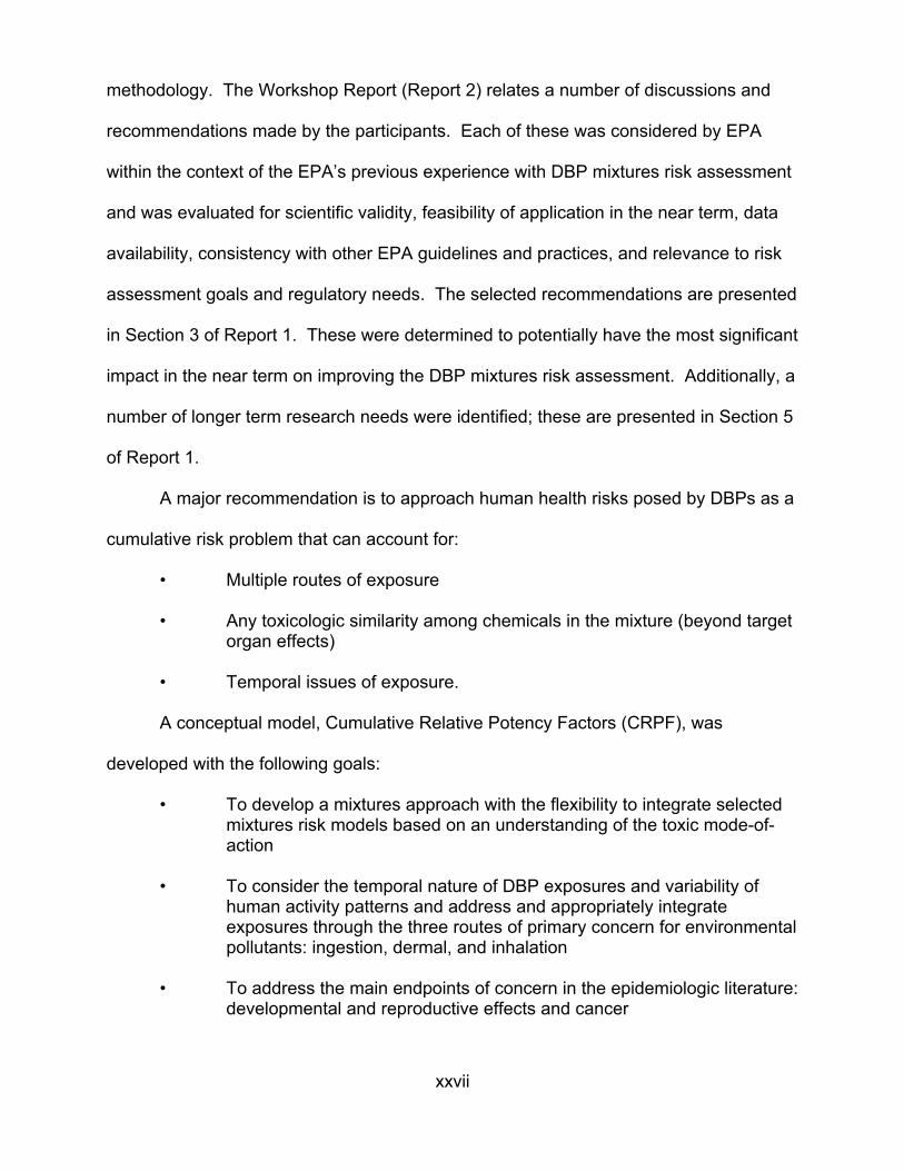
methodology. The Workshop Report (Report 2) relates a number of discussions and
recommendations made by the participants. Each of these was considered by EPA
within the context of the EPA’s previous experience with DBP mixtures risk assessment
and was evaluated for scientific validity, feasibility of application in the near term, data
availability, consistency with other EPA guidelines and practices, and relevance to risk
assessment goals and regulatory needs. The selected recommendations are presented
in Section 3 of Report 1. These were determined to potentially have the most significant
impact in the near term on improving the DBP mixtures risk assessment. Additionally, a
number of longer term research needs were identified; these are presented in Section 5
of Report 1.
A major recommendation is to approach human health risks posed by DBPs as a
cumulative risk problem that can account for:
• Multiple routes of exposure
• Any toxicologic similarity among chemicals in the mixture (beyond target organ effects)
• Temporal issues of exposure.
A conceptual model, Cumulative Relative Potency Factors (CRPF), was
developed with the following goals:
• To develop a mixtures approach with the flexibility to integrate selected mixtures risk models based on an understanding of the toxic mode-of-action
• To consider the temporal nature of DBP exposures and variability of human activity patterns and address and appropriately integrate exposures through the three routes of primary concern for environmental pollutants: ingestion, dermal, and inhalation
• To address the main endpoints of concern in the epidemiologic literature: developmental and reproductive effects and cancer
xxvii
• To identify the “risk-relevant” components of DBP mixtures. This may include organic halides that are not measured individually as well as DBPs that are not halogenated
• To estimate risks for various drinking water treatment trains, reflecting differences in the DBPs formed and their concentrations over time in the distribution system
• To generate central tendency risk estimates along with their associated probability distributions; such distributions of risks are needed to appropriately reflect both the uncertainty and variability found in these data
• To identify specific measures to incorporate into future epidemiologic investigations that could improve exposure classification
• To develop mixtures risk characterization approaches to be used in the evaluation of causality.
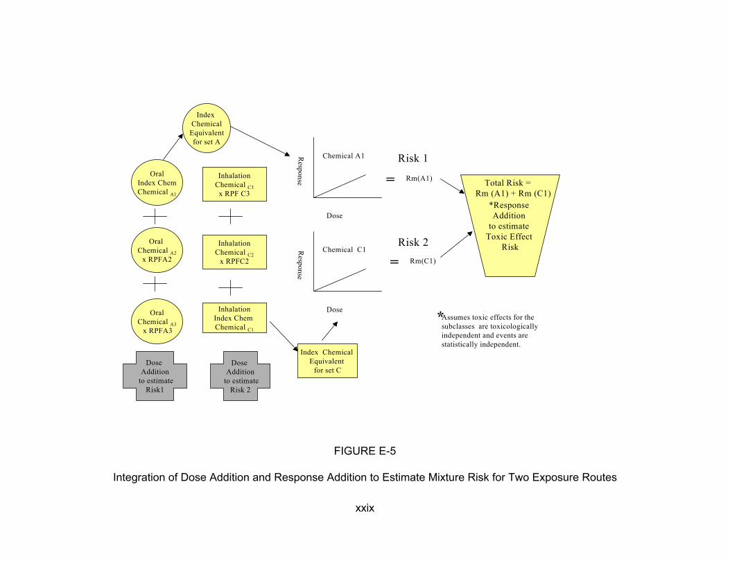
The goal of the conceptual approach is the integration across routes of Relative
Potency Factor (RPF)-based risk estimates (U.S. EPA, 2000a) that are route-specific for
toxicologically similar subclasses of DBPs for an effect-specific period of duration.
Once several RPF risk estimates are generated, then the analyst can make some
assumptions relative to the likely relationships of the across-subclass risks and
determine if and how the subclasses should be combined (e.g., a response addition
assumption would lead to summing these RPF risks) to estimate the total risk estimate
for the mixture (Figure E-5). This approach is designed to produce a transparent
cumulative risk assessment because assumptions about the toxicity and the interactions
must be specifically identified.
The RPF approach has been proposed as an interim approach for characterizing
health risks associated with mixtures of chemical compounds that have data indicating
that they are toxicologically similar (U.S. EPA, 1999c). To develop an RPF-based
xxviii
Oral Index Chem Chemical A1
Inhalation Chemical C3
x RPF C3
Index Chemical
Equivalent for set A
Chemical A1
Rm(A1)=
Dose
Oral Chemical A2
x RPFA2
Risk 2Inhalation Chemical C2
x RPFC2
Inhalation Index Chem Chemical C1
Dose Addition
to estimate Risk 2
Index hemical Equivalent
for set C
Dose
Response
Chemical C1
C
Rm(C1)=
*Response Addition
to estimate Toxic Effect
Risk
Total Risk = Rm (A1) + Rm (C1)
Oral Chemical A3
x RPFA3 *Assumes toxic effects for the
subclasses are toxicologically independent and events are statistically independent.
Dose Addition
to estimate Risk1
FIGURE E-5
Integration of Dose Addition and Response Addition to Estimate Mixture Risk for Two Exposure Routes
xxix
Risk 1Response

risk estimate for a class of chemicals, toxicologic data are needed at least for one
component of the mixture (referred to as the index chemical), and scientific judgment is
used to assess the relative toxicity of the other individual components in the mixture as
well as of the mixture as a whole. The RPF approach assumes dose addition is
appropriate for the related components that comprise the mixture or a subset of the
mixture components. True dose addition assumes that the components of the mixture
act by the same mode of action. The exposure level of each component in the mixture
is scaled by its toxicity relative to that of the index chemical, resulting in an index
chemical equivalent dose for each component (e.g., the columns of circles or rectangles
in Figure E-5). This scaling factor (the RPF) is based on a comparison of relevant dose-
response information between the index chemical and the component, including the
results of toxicologic assays and analyses of structural similarity to other compounds of
known toxicologic potential. For each component of the mixture, the RPF approach
predicts an equivalent exposure in terms of the index chemical; these equivalent
exposures are then summed to generate an index chemical-equivalent total mixture
dose. The risk posed by the mixture is then estimated using the dose-response curve
of the index chemical.
The development of RPF-based risk estimates and their integration with
response addition in a CRPF approach addresses many of the shortcomings of the first
response addition assessment; not all issues are addressed, however. The approach
does not directly address the differences in risks for sensitive subpopulations or the
contribution to the risk estimate that may be addressed by using what is known in the
epidemiologic literature. In addition, application of CRPF promises to be a resource-
intensive exercise that may be more technically correct than the application of response
xxx
addition, but, in the end, may not produce risk estimates very different in magnitude.
Furthermore, an enormous problem lies in the fact that very few toxicity data are
available for the dermal and inhalation routes of exposure.
The CRPF approach is a conceptual model for development of a cumulative risk
assessment for DBP mixtures. It improves upon the initial response addition
assessment by more carefully considering toxicologic similarities among chemicals,
route of exposure, and physiologically-relevant time frames. It allows treatment system-
specific exposures to be investigated and, although not specified in this discussion,
does not preclude the use of human activity patterns and distribution system effects
from being incorporated into the analysis. Risk estimates for the unidentified DBPs can
also be included in the development of the RPF-based risk estimates. A probabilistic
analysis and full risk characterization would be required with careful treatment of the
variabilities and uncertainties examined and explained.
In summary, investigations into the potential human health risks from DBP
mixture exposures are important to conduct because of both the ubiquitous nature of
the exposures and the evidence of health effects in both the epidemiology and
toxicology literature. In this research effort, we have made the following progress:
• NCEA-Cin has performed an assessment of human health risks for developmental and reproductive effects and cancer from exposure to DBP mixtures (Appendix I), using a response addition approach that incorporates data on the unidentified fraction of the DBPs and uses a probabilistic approach.
• NCEA-Cin has produced a workshop report (Report 2) that contains a wealth of information on the exposure, dose-response and risk characterization issues relative to DBP mixtures health risks that can be used by risk assessors interested in this area.
• NCEA-Cin has developed a new conceptual approach (Report 1), the Cumulative Relative Potency Factors (CRPF) method, for assessing
xxxi
DBP mixtures health risks. The CRPF method improves on the response addition method by integrating data on mode of action and multiple routes of exposure over physiologically-relevant time frames.
• NCEA-Cin has recommended areas of research most critical for improving DBP mixtures health risk assessment (Report 1).
Improvements in the development of health risk estimates are needed, with the
most important scientific directions to include:
• Integration of both human and animal toxicity data into the assessment
• Development of exposure models that incorporate dermal, oral and inhalation routes, human activity patterns, and measures of internal dose
• Collection of concentration data that are representative of real world drinking water samples, including additional information on the unidentified fraction of the DBPs
• Application of risk characterization methods that incorporate data on the toxic mode of action for the physiologically-relevant exposure time frame
• Consideration of sensitive subgroups in the population
• Analysis of variability in the data and uncertainty of the final risk estimates.
Research that addresses these improvements will be valuable not only to the
human health risk assessment of DBP mixtures, but also to the advancement of
chemical mixtures risk assessment methodology applicable to other environmental
exposures.
xxxii
1. INTRODUCTION
1.1. PURPOSE
The risk assessment of disinfection by-product (DBP) mixtures in drinking water
addresses an important issue in environmental health and also facilitates risk
assessment methods development. To improve its assessment of the DBP mixture
health risk, NCEA-Cin has been exploring a number of novel approaches to generating
realistic, central tendency estimates of potential health risks, despite data limitations
and uncertainties. These include such risk characterization methods and adjuncts such
as response addition, proportional-response addition, relative potency factors,
dosimetry, quantitative structure activity relationships, development of distributions for
relevant variables, and Monte Carlo simulation. The purpose of this document (i.e.,
Report 1, Report 2, and Appendix I) is to detail the response addition method that was
initially developed to estimate DBP mixtures risk, discuss the state of DBP toxicity and
exposure data, present available methods for mixtures risk characterization that may be
applicable, explore alternative methodologies, and make recommendations for future
applications and methodological developments.
The need to study the conduct of a risk assessment for DBP mixtures arose both
as a mandate and also as a logical scientific direction. Under 42 USC § 300 of the Safe
Drinking Water Act Amendments of 1996, it is stated that the EPA will “develop new
approaches to the study of complex mixtures, such as mixtures found in drinking
water...” In addition, the EPA’s Office of Water drafted a Research Plan for Microbial
Pathogens and DBPs in Drinking Water that calls for the characterization of DBP
R1-1 03/08/2001
mixtures risk (U.S. EPA, 1997a). In response to these mandates, NCEA-Cin began
investigating the DBP mixture issue and identified a number of scientific interests,
including: developing a method to compare DBP risks across various drinking water
treatment interventions; evaluating potential drinking water health risks by comparing
and integrating toxicology and epidemiology data; and furthering the development of
mixtures risk assessment methods for general use in evaluating environmental
problems.
1.2. STRUCTURE OF THE DOCUMENT
This effort has resulted in the production of three interrelated research reports
and an external review report that are contained in this document as follows:
• Report 1, September, 2000: EPA’s conclusions, recommendations, conceptual approach and future directions regarding the conduct of a DBP mixture risk assessment. Although new information and ideas not in Report 2 or Appendix I are included, Report 1 is not written as a stand-alone document; it is meant to be read in conjunction with Report 2 and Appendix I.
• Report 2, January, 2000: Summary of presentations and discussions at an April 1999 workshop where scientists examined an illustrative example of a DBP mixtures risk assessment, presented ideas to advance the approach, and recommended research and development directions.
• Appendix I, April, 1999: The illustrative example of a DBP mixtures risk assessment (using a response addition approach) developed by NCEA-Cin, including data, assumptions and statistical methods used. Shows resulting risk distributions and uncertainty analysis.
• Appendix II, July, 2000: External scientific review of the Research Report. Comments and recommendations are concentrated primarily on Report 1 of this document.
R1-2 03/08/2001

Figure 1 illustrates the process NCEA-Cin has followed to produce this document
and projects subsequent activities in this research area. The initial assessment of the
project in December 1998 (U.S. EPA, 1998a) was subsequently developed into a pre-
meeting report for the April 1999 workshop on this subject entitled: Workshop Pre-
Meeting Report: The Risk Assessment of Mixtures of Disinfection By-Products (DBPs)
for Drinking Water Treatment Systems (U.S. EPA, 1999a) Appendix 1 details the
response addition approach to estimating DBP mixture risk. During this initial
assessment, NCEA-Cin scientists recognized a number of areas for improvement and
held the April 1999 workshop to examine the response addition method, present ideas
to advance the approach, and generate some conclusions relative to new research and
development directions. The resulting workshop report is presented as Report 2
entitled: Workshop Report: Novel Methods for Risk Assessment of Mixtures of
Disinfection By-Products (DBPs) for Drinking Water Treatment Systems. Finally, based
on information developed in the April 1999 workshop, EPA scientists reached a number
of conclusions relative to this area of research and developed an approach to the
assessment of cumulative risk. This information is presented as Report 1, entitled EPA
Conclusions and Conceptual Approach for Conducting a Risk Assessment of Mixtures
of Disinfection By-Products (DBPs) for Drinking Water Treatment Systems. Report 1 is
a composite document linked to Report 2 and Appendix I by pointers within the text to
provide the reader with additional information on a topic area. Appendix II contains the
external review report entitled: Peer Review of the “Research Report: The Risk
Assessment of Mixtures of Disinfection Byproducts (DBPs) for Drinking Water
R1-3 03/08/2001
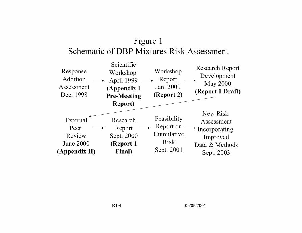
Figure 1Schematic of DBP Mixtures Risk Assessment
Scientific Workshop Research ReportResponse Workshop
Addition April 1999 Report Development May 2000Assessment
Pre-Meeting Report)
(Report 2)
Research New Risk
Feasibility
(Appendix I Jan. 2000 (Report 1 Draft)Dec. 1998
External Assessment Report Report onPeer
Sept. 2000 Cumulative Incorporating
Review ImprovedJune 2000 (Report 1 Risk Data & Methods
(Appendix II) Final) Sept. 2001 Sept. 2003
R1-4 03/08/2001
Treatment Systems.” As indicated in Figure 1, additional research and assessment
work on DBP mixtures risk assessment is ongoing.
1.3. BACKGROUND
The authors of this document have chosen to evaluate DBP health effects using
mixture risk assessment approaches, rather than assessing each individual chemical
separately. These approaches acknowledge real human exposures, as well as account
for any compounded effects from exposure to the low levels of multiple DBPs found in
drinking water. Because toxic effects have not been observed in animal studies when
the exposures are to low doses of DBPs and because the epidemiologic data are
inconsistent across studies with only relatively weak to moderate associations noted,
the existence of human health risks is questionable, but cannot be entirely dismissed.
If it is assumed, however, that the human health effects suggested in some
epidemiologic studies are real, then several hypotheses can be posed to explain the
discrepancies between the epidemiologic results and the lack of effects in animals
exposed to finished drinking water (i.e., water that has undergone a disinfection
process). Such hypotheses include the following:
• There is an effect from exposure to the mixture of DBPs that is at least additive (if not synergistic) in nature, so that toxicology studies involving low levels of individual DBPs are inadequate to explain the health effects found in the positive epidemiologic data
• Effects in humans are the result of chronic, repetitive insult from daily exposure to DBP mixtures; effects in humans may occur only in sensitive individuals who are genetically predisposed or in high end consumers of drinking water
• Laboratory animals differ from humans in physiology, biochemistry, anatomy, genetic heterogeneity and lifestyle factors (e.g., high fat diets) that prevent demonstration of the same health outcomes across species
R1-5 03/08/2001

• Laboratory studies to date expose animals by only a single route, usually oral, so that effects resulting from a combined oral-dermal-inhalation exposure are not observed
• Effects in epidemiologic studies are the result of exposure to other environmental contaminants, such as metals, inorganic materials or pesticides in the drinking water, so that animal studies solely focused on DBPs will not corroborate epidemiologic findings.
Although it may be noted that these hypotheses are not mutually exclusive, the authors
of this document have chosen the first hypothesis (that adverse health effects exist and
are attributable to exposure to the complex mixture) as the basic premise on which to
build a risk assessment approach.
The specific goals of the DBP mixtures risk assessment are the following:
• To compare DBP risks for drinking water treatment trains that reflect differences in DBP production and concentrations
• To make reasonable risk estimates for all endpoints of concern because of suggested cancer, reproductive and developmental effects in the epidemiologic literature
• To develop distributions of risks that reflect their uncertainty and variability for use in sensitivity analyses
• To incorporate information on both the unknown and known DBPs into the risk estimate.
The response addition approach (Section 2.5. of this report and Appendix I) was
used as a first step in this process, although a number of factors were not addressed.
Specifically, this initial assessment:
• Did not address multiple exposure routes (dermal, oral, inhalation)
• Did not assess multiple time frames or physiologically relevant time frames
• Did not use epidemiologic data for quantitative risk assessment
R1-6 03/08/2001
• Did not take into account human activity patterns to adjust exposure
• Did not make dosimetric adjustments to account for toxic mode of action, including consideration of pharmacokinetic and pharmacodynamic determinants of observed effect
• Did not address unidentified by-products of disinfection other than organic halides;
• Dd not use alternative Quantitative Structure Activity Relationship models in assessing potential toxicity of unidentified compounds
• Did not utilize alternative mixtures risk characterization models to derive estimates of risk.
These topics were addressed in the April 1999 workshop (Report 2) and have become
the basis for proposing a new conceptual model for assessing DBP mixture risk.
R1-7 03/08/2001

2. SUMMARY: CURRENT STATE OF THE SCIENCE
2.1. INTRODUCTION
Humans are exposed concurrently and sequentially to chemical mixtures at
various exposure levels. The by-products formed during chemical disinfection of water
present an example of multiple chemical, multiple route exposure that is ubiquitous
across all segments of the U.S. population, as well as the populations of many
developed countries around the world. Human exposure to the chemicals formed as
by-products of chemical disinfection of water is an example of both a concurrent
exposure to a complex mixture of chemicals (the mixture of chemicals in the glass of
water consumed today) and a temporally separated mixtures exposure (exposure to the
DBPs in the glass of water consumed today is temporally separated from the DBPs
consumed yesterday, as well as from the DBPs encountered during bathing in the
morning).
The health benefits of chemical disinfection, i.e., dramatic decreases in both
morbidity and mortality from water-borne diseases, are clearly evident (Regli et al.,
1993). A consequence of water disinfection however, is low-level exposure to myriad
DBPs. Disinfectants such as free chlorine, combined chlorine (monochloramine),
ozone, and chlorine dioxide [the most common oxidants and disinfectants used (Singer,
1995)] react with naturally occurring organic and inorganic material in the incoming
source water to produce a variety of DBPs. A number of factors influence the formation
of DBPs: the type, concentration and point of application of the disinfectant; the type
and concentration of organic and inorganic precursor material; the disinfectant contact
R1-8 03/08/2001
time; and source water characteristics of pH, bromide concentration and temperature
(Singer, 1995; Fair, 1995). Several hundred chemically distinct DBPs have been
identified in the laboratory but, in general, approximately 50% of the DBPs is made up
of an unknown number of unidentified chemicals (Miltner et al., 1990; Richardson, 1998;
Weinberg, 1999).
Human health risks from exposure to DBPs are of concern; both the
epidemiologic and toxicologic literature provide some evidence of potential adverse
health effects. Taken as a whole, epidemiologic studies on chlorinated drinking water
offer some evidence of an association with certain cancers, and reproductive and
developmental effects, warranting further investigation. In contrast, in whole mixture
studies, toxic effects have not been observed when animals are exposed to finished
drinking water, but there is evidence of mutagenicity in in vitro studies of drinking water
extracts and concentrates. In in vivo studies at high doses of individual DBPs and some
defined DBP mixtures, there is evidence of carcinogenicity, reproductive and
developmental effects, nephrotoxicity and hepatotoxicity. Thus, the existence of
adverse human health effects from exposure to environmental levels of DBPs is
certainly possible, but also highly uncertain.
2.1.1. Risk Assessment Paradigm for DBP Mixtures. The EPA generally follows the
paradigm established by the National Academy of Sciences (NRC, 1983) when
performing a human health risk assessment. This paradigm consists of a group of
interrelated processes: hazard identification, dose-response assessment, exposure
assessment and risk characterization. These processes are also the basis for the
R1-9 03/08/2001

current DBP mixtures risk assessment and are the elements that must be addressed in
making improvements. These elements are described briefly as follows:
1) Hazard Identification. Available data on biological endpoints are used to determine
if the DBPs are likely to pose a hazard to human health. These data are also used to
define the type of potential hazard, its severity, and the modes of action associated with
the chemicals of interest. For mixtures, hazard identification must also consider
potential interaction effects from exposure to the combination of DBPs and their
combined doses.
2) Dose-Response Assessment. Data are used to estimate the concentrations of
DBPs that may elicit an adverse effect in humans. The risk assessor may define a
quantitative dose-response relationship usable for low dose exposure, often by applying
mathematical models to the data. For mixtures, dose-response assessment must
consider the potential for effects below individual chemical thresholds as well as
incorporate judgments related to similarity of mode-of-action within or between mixtures.
3) Exposure Assessment. Exposure assessment uses available data relevant to
population exposure, such as concentration data, tap water consumption patterns, and
biomarker information to determine the extent to which a population is exposed to
DBPs. Fate and transport of the DBPs in the environment, routes of exposure,
pharmacokinetics and pharmacodynamics of the DBPs once in the body may all be
considered in the exposure assessment. For mixtures, exposure assessment must take
into account chemical characterization of unidentified DBPs in the complex mixture and
the variability of the mixture in the distribution system over time.
R1-10 03/08/2001

4) Risk Characterization. This step in the paradigm summarizes assessments of
human health, identifies human sub-populations at elevated risk, assesses exposures
from multiple environmental media and describes the uncertainty and variability in these
assessments. For mixtures, risk characterization must evaluate how well the
assumptions made about interaction effects, toxicologic similarity of mixtures or their
components, and exposure can be supported by the data. In both the exposure
assessment and the dose-response assessment steps for a chemical mixtures risk
assessment, the analyst must determine whether the mixture evaluated in the
laboratory is “sufficiently similar” to the mixture encountered in the environment. This
judgement of sufficient similarity between the “tested” mixture and the “environmental”
mixture is a unique element of the risk characterization step in the chemical mixtures
risk assessment paradigm.
2.2. MIXTURES RISK ASSESSMENT METHODS
The EPA began to address concerns over health risks from multiple chemical
exposures in the 1980s and issued its Guidelines for the Health Risk Assessment of
Chemical Mixtures in 1986 (U.S. EPA, 1986). Continued interest and research in this
area and in multiple route exposures has resulted in other documents over the years
(U.S. EPA, 1989a, 1989b, 1990, 1999b). In 2001, the EPA is expected to release
further guidance on the assessment of risks posed by exposures to chemical mixtures
(U.S. EPA. 1999c; 2000a). A number of publications provide additional depth and
information on chemical mixtures toxicology and risk assessment methods for complex
mixtures (see, e.g., Cassee et al., 1998; Hertzberg et al., 1999; Krishnan and Brodeur,
R1-11 03/08/2001

1991; Mumtaz et al., 1997a, 1998; NRC, 1988; Simmons, 1995a; Svendsgaard and
Hertzberg, 1994; Teuschler and Hertzberg, 1995; Yang, 1994; Yang and Suk, 1998).
2.2.1. Key Concepts. Several important concepts have evolved relative to the
evaluation of chemical mixtures (U.S. EPA, 1999c). The first is the role of toxicologic
similarity which can be considered along a spectrum of information on toxicologic action
from mechanism-of-action, specific molecular understanding of a toxicologic process
(e.g., DNA damage due to adduct formation), to mode-of-action, a more general
understanding of these processes at the tissue level in the body (e.g., centrilobular
necrosis of the liver), to toxicologic similarity, toxicologic action expressed in broad
terms such as at the target organ level (e.g., enzyme changes in the liver).
Assumptions about toxicologic similarity play an important role in chemical risk
assessment evaluations.
The second key concept is the assumption of similarity or, in contrast,
independence of action. The term, sufficiently similar mixture, refers to a mixture very
close in composition to the mixture of concern; differences in their components and their
proportions are small; and the data from the sufficiently similar mixture can be used to
estimate risk for the mixture of concern. The term, similar components, refers to the
single chemicals within a mixture that act by the same mode-of-action and may have
comparable dose-response curves; a component-based risk assessment can be
performed. The term, group of similar mixtures, refers to chemically-related classes of
mixtures that act by a similar mode-of-action, have closely related chemical structures,
and occur together routinely in environmental samples, usually because they are
generated by the same commercial process or remain after environmental
R1-12 03/08/2001
transformation; chemical mixtures risk assessments are conducted using knowledge
about the shifts in chemical structure and relative potency of the components. Finally,
the term, independence of action, refers to a group of mixture components for which the
toxicity caused by any single component is not influenced by the toxicity of the other
components; the probabilities of toxic effects for the individual components can be
combined.
The third key concept is understanding language referring to toxicologic
interactions, defined here as any toxic responses that are greater than or less than what
is observed under an assumption of additivity. The term, additivity, is used when the
effect of the combination of chemicals can be estimated directly from the sum of the
exposure levels (dose addition), the sum of the responses (response addition) of the
individual components, or the sum of the biological effects of the individual components
(effects addition). The most general terms for interaction effects are synergism (i.e.,
greater than additive) and antagonism (i.e., less than additive).
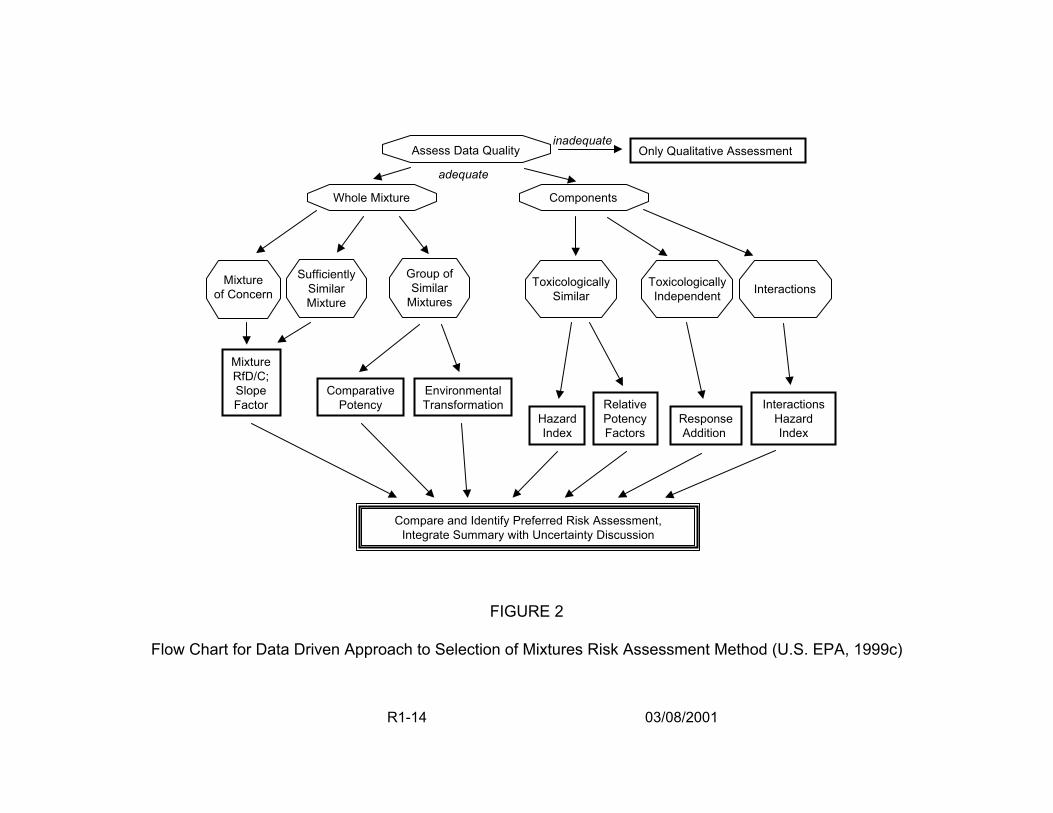
2.2.2. Data-Driven Approaches for Assessing Risks Posed by Chemical Mixtures.
Figure 2 (U.S. EPA, 1999c) describes the selection of a chemical mixture risk
assessment method, beginning with an assessment of data quality and availability and
progressing to a number of judgments relative to data type, chemical composition, and
toxicologic activity to choose among risk assessment methods. The major concerns are
whether the available data are on components or whole mixtures; whether the data are
composed of either similar components or similar mixtures that can be viewed as acting
by similar toxicologic processes; whether the mixture components act by the same
mode of action or are functionally independent; and whether the data may be
R1-13 03/08/2001
Mixture of Concern
Assess Data Quality inadequate
Only Qualitative Assessment
adequate
Whole Mixture Components
Sufficiently Similar Mixture
Toxicologically Similar
Toxicologically Independent
Potency Factors Index
Response Addition
Compare and Identify Preferred Risk Assessment, Integrate Summary with Uncertainty Discussion
RfD/C; Slope Comparative Environmental Factor Potency Transformation Relative Interactions
Hazard Hazard Index
Interactions Group of Similar
Mixtures
Mixture
FIGURE 2
Flow Chart for Data Driven Approach to Selection of Mixtures Risk Assessment Method (U.S. EPA, 1999c)
R1-14 03/08/2001

grouped by emissions source, chemical structure or biologic activity. The results of
such judgments point the risk assessor toward methods that are available for these
specific types of data. Methods selected for whole mixtures depend on whether
information is directly available on the mixture of concern or only on sufficiently similar
mixtures or groups of similar mixtures. Methods available for component data depend
on whether data on interactions are available, or whether the components act with a
similar mode of action or are toxicologically independent. For all assessments based on
data of adequate quality, the outcome is a quantitative assessment with a complete risk
characterization and uncertainty discussion presented. Tables 1 and 2 contain short
descriptions for many of the available methods indicated as endpoints in Figure 2, with
references for further information.
Figure 2 is deceptively simple, as many of the issues presented in the diagram
depend on scientific judgment or data that may not be readily available. In addition,
there will often be mixtures for which whole mixture data and component data both
exist, so the choice of method will not be clear (for example, both epidemiologic data
and component toxicity data may exist). Furthermore, the true toxicologic mechanism-
of-action is rarely known for a given mixture or even for most of its components; the
judgments made of toxicologic similar action or independence of action, for example,
will be uncertain. Thus, one approach that the risk assessor can take is to implement
several of the methods that are practical to apply and evaluate the range of health risk
estimates that are produced.
2.2.3. Risk Characterization and Uncertainty. Mixtures risk characterization requires
the use of considerable judgment along with plausible approaches that must be
R1-15 03/08/2001
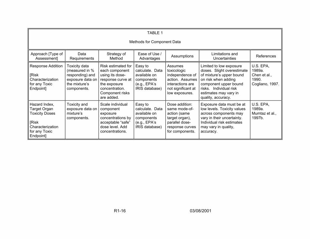
TABLE 1
Methods for Component Data
Approach [Type of Assessment]
Data Requirements
Strategy of Method
Ease of Use / Advantages Assumptions Limitations and
Uncertainties References
Response Addition [Risk Characterization for any Toxic Endpoint]
Toxicity data (measured in % responding) and exposure data on the mixture’s components.
Risk estimated for each component using its dose-response curve at the exposure concentration. Component risks are added.
Easy to calculate. Data available on components (e.g., EPA’s IRIS database)
Assumes toxicologic independence of action. Assumes interactions are not significant at low exposures.
Limited to low exposure doses. Slight overestimate of mixture’s upper bound on risk when adding component upper bound risks. Individual risk estimates may vary in quality, accuracy.
U.S. EPA, 1989a. Chen et al., 1990. Cogliano, 1997.
Hazard Index, Target Organ Toxicity Doses [Risk Characterization for any Toxic Endpoint]
Toxicity and exposure data on mixture’s components.
Scale individual component exposure concentrations by acceptable “safe” dose level. Add concentrations.
Easy to calculate. Data available on components (e.g., EPA’s IRIS database)
Dose addition: same mode-of-action (same target organ), parallel dose-response curves for components.
Exposure data must be at low levels. Toxicity values across components may vary in their uncertainty. Individual risk estimates may vary in quality, accuracy.
U.S. EPA, 1989a. Mumtaz et al., 1997b.
R1-16 03/08/2001
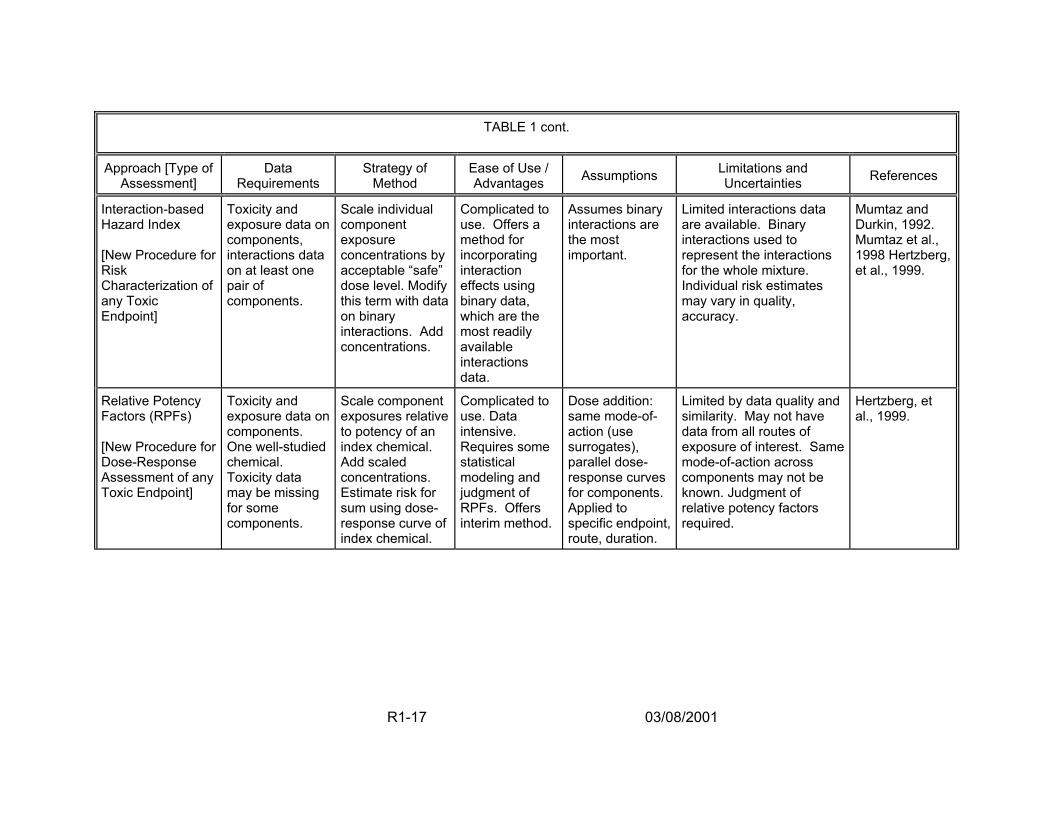
TABLE 1 cont.
Approach [Type of Assessment]
Data Requirements
Strategy of Method
Ease of Use / Advantages Assumptions Limitations and
Uncertainties References
Interaction-based Hazard Index [New Procedure for Risk Characterization of any Toxic Endpoint]
Toxicity and exposure data on components, interactions data on at least one pair of components.
Scale individual component exposure concentrations by acceptable “safe” dose level. Modify this term with data on binary interactions. Add concentrations.
Complicated to use. Offers a method for incorporating interaction effects using binary data, which are the most readily available interactions data.
Assumes binary interactions are the most important.
Limited interactions data are available. Binary interactions used to represent the interactions for the whole mixture. Individual risk estimates may vary in quality, accuracy.
Mumtaz and Durkin, 1992. Mumtaz et al., 1998 Hertzberg, et al., 1999.
Relative Potency Factors (RPFs) [New Procedure for Dose-Response Assessment of any Toxic Endpoint]
Toxicity and exposure data on components. One well-studied chemical. Toxicity data may be missing for some components.
Scale component exposures relative to potency of an index chemical. Add scaled concentrations. Estimate risk for sum using dose-response curve of index chemical.
Complicated to use. Data intensive. Requires some statistical modeling and judgment of RPFs. Offers interim method.
Dose addition: same mode-of-action (use surrogates), parallel dose-response curves for components. Applied to specific endpoint, route, duration.
Limited by data quality and similarity. May not have data from all routes of exposure of interest. Same mode-of-action across components may not be known. Judgment of relative potency factors required.
Hertzberg, et al., 1999.
R1-17 03/08/2001
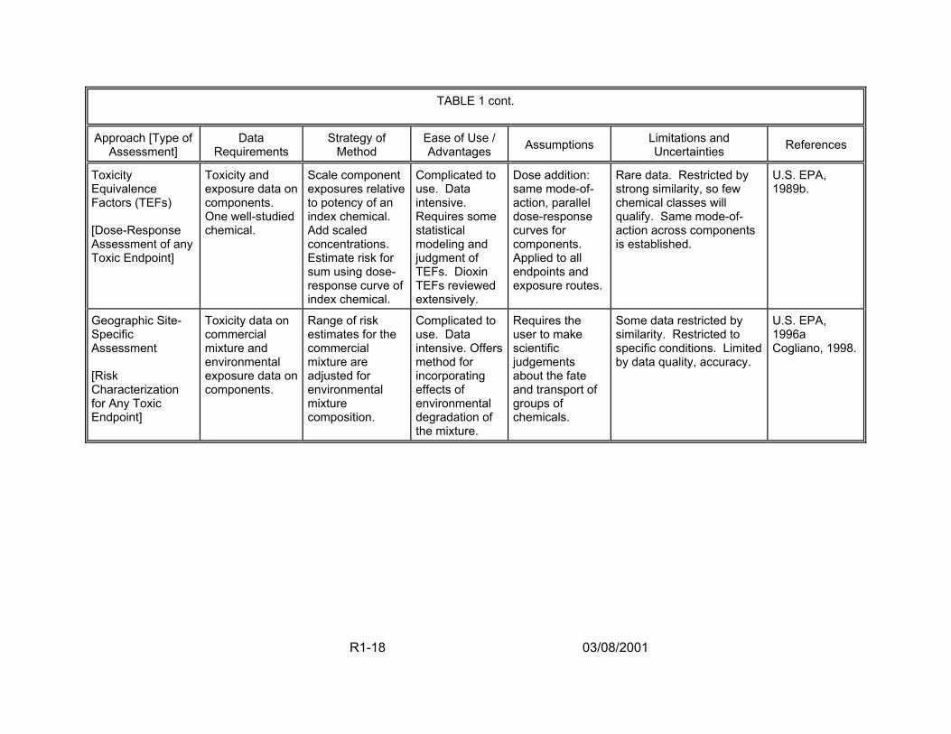
TABLE 1 cont.
Approach [Type of Assessment]
Data Requirements
Strategy of Method
Ease of Use / Advantages Assumptions Limitations and
Uncertainties References
Toxicity Equivalence Factors (TEFs) [Dose-Response Assessment of any Toxic Endpoint]
Toxicity and exposure data on components. One well-studied chemical.
Scale component exposures relative to potency of an index chemical. Add scaled concentrations. Estimate risk for sum using dose-response curve of index chemical.
Complicated to use. Data intensive. Requires some statistical modeling and judgment of TEFs. Dioxin TEFs reviewed extensively.
Dose addition: same mode-of-action, parallel dose-response curves for components. Applied to all endpoints and exposure routes.
Rare data. Restricted by strong similarity, so few chemical classes will qualify. Same mode-of-action across components is established.
U.S. EPA, 1989b.
Geographic Site-Specific Assessment [Risk Characterization for Any Toxic Endpoint]
Toxicity data on commercial mixture and environmental exposure data on components.
Range of risk estimates for the commercial mixture are adjusted for environmental mixture composition.
Complicated to use. Data intensive. Offers method for incorporating effects of environmental degradation of the mixture.
Requires the user to make scientific judgements about the fate and transport of groups of chemicals.
Some data restricted by similarity. Restricted to specific conditions. Limited by data quality, accuracy.
U.S. EPA, 1996a Cogliano, 1998.
R1-18 03/08/2001
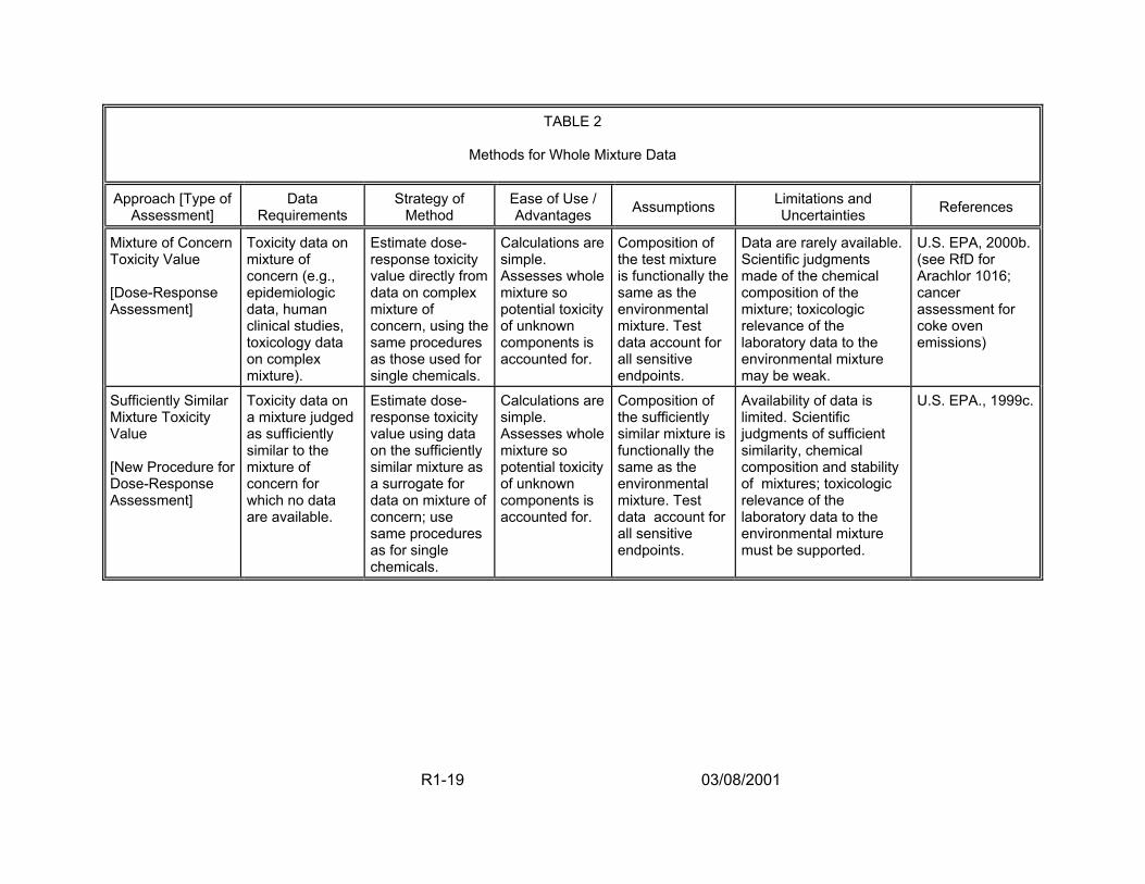
TABLE 2
Methods for Whole Mixture Data
Approach [Type of Assessment]
Data Requirements
Strategy of Method
Ease of Use / Advantages Assumptions Limitations and
Uncertainties References
Mixture of Concern Toxicity Value [Dose-Response Assessment]
Toxicity data on mixture of concern (e.g., epidemiologic data, human clinical studies, toxicology data on complex mixture).
Estimate dose-response toxicity value directly from data on complex mixture of concern, using the same procedures as those used for single chemicals.
Calculations are simple. Assesses whole mixture so potential toxicity of unknown components is accounted for.
Composition of the test mixture is functionally the same as the environmental mixture. Test data account for all sensitive endpoints.
Data are rarely available. Scientific judgments made of the chemical composition of the mixture; toxicologic relevance of the laboratory data to the environmental mixture may be weak.
U.S. EPA, 2000b. (see RfD for Arachlor 1016; cancer assessment for coke oven emissions)
Sufficiently Similar Mixture Toxicity Value [New Procedure for Dose-Response Assessment]
Toxicity data on a mixture judged as sufficiently similar to the mixture of concern for which no data are available.
Estimate dose-response toxicity value using data on the sufficiently similar mixture as a surrogate for data on mixture of concern; use same procedures as for single chemicals.
Calculations are simple. Assesses whole mixture so potential toxicity of unknown components is accounted for.
Composition of the sufficiently similar mixture is functionally the same as the environmental mixture. Test data account for all sensitive endpoints.
Availability of data is limited. Scientific judgments of sufficient similarity, chemical composition and stability of mixtures; toxicologic relevance of the laboratory data to the environmental mixture must be supported.
U.S. EPA., 1999c.
R1-19 03/08/2001
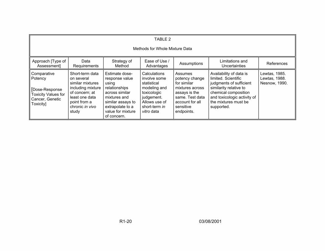
TABLE 2
Methods for Whole Mixture Data
Approach [Type of Assessment]
Data Requirements
Strategy of Method
Ease of Use / Advantages Assumptions Limitations and
Uncertainties References
Comparative Potency [Dose-Response Toxicity Values for Cancer, Genetic Toxicity]
Short-term data on several similar mixtures including mixture of concern; at least one data point from a chronic in vivo study
Estimate dose-response value using relationships across similar mixtures and similar assays to extrapolate to a value for mixture of concern.
Calculations involve some statistical modeling and toxicologic judgement. Allows use of short-term in vitro data
Assumes potency change for similar mixtures across assays is the same. Test data account for all sensitive endpoints.
Availability of data is limited. Scientific judgments of sufficient similarity relative to chemical composition and toxicologic activity of the mixtures must be supported.
Lewtas, 1985. Lewtas, 1988. Nesnow, 1990.
R1-20 03/08/2001
presented transparently. Mixtures composed of chemicals thought to have threshold
effects must be assessed and presented carefully. A common interpretation is that
mixtures with few components, each less than its respective threshold, pose no
significant risk. For chemicals acting by the same mode-of-action, this conclusion can
be in error because the joint exposures contribute to the same potential toxicity and
effectively represent a cumulative dose. Thus, a dose-additive assessment should be
performed (i.e., summing the component doses that are scaled for potency and
estimating the risk for the total mixture dose). For a mixture of toxicologically dissimilar
chemicals thought to be functionally independent, an assessment can be performed
using response addition (i.e., summing the risks of the individual components). In this
case, the mixture risk would likely be judged negligible, particularly if the threshold
effects are considered minor. When the toxic effects are of major concern, such as
cancer or developmental toxicity, the estimated mixture risk should be judged in the
context of the effects, the shapes of the dose-response curves, and the characteristics
of the exposed population (U.S. EPA, 1999c).
Whenever an assessment is based on component toxicity values, the risk
characterization must discuss the quality of the individual chemical estimates used,
including both exposure data and dose-response information. For example, cancer
potency estimates are uncertain, as reflected by confidence levels and goodness-of-fit
values when dose-response models are applied, as well as by qualitative descriptors of
the weight of evidence that the chemical is a human carcinogen. Similarly, human
exposure estimates can be uncertain because of water treatment system practices,
source water characteristics or tap water consumption patterns. All these measures of
R1-21 03/08/2001

uncertainty and unevenness of component estimates must be described, at least in
summary fashion, in the risk characterization.
Many of the variables that are quantified in a mixtures risk assessment can have
multiple possible values, resulting in a need to address both variability and uncertainty
when applying the methodology. First, a parameter’s true value may be uncertain but
may not vary across individuals in the population. In this case, the parameter has one
true value for all individuals in the population but that value is not known. Second, a
parameter’s value may vary across individuals in the population but be treated as
known with certainty. It is important to segregate the influence of uncertainty and
variability because they give rise to two different sets of questions. Uncertainty raises
the question of how precise the resulting risk estimates are. Variability raises the
question of whether there are (identifiable) individuals in the population at a particularly
elevated risk. Application of a probabilistic approach allows the results of an analysis to
be used to quantify the distribution of plausible risks for the population. To implement
the analysis, input distributions are developed for all variables thought to be variable or
uncertain; such distributions are developed to reflect best estimates of the variables for
use in simulations and should not be biased toward conservative estimates of risk.
Following the generation of a distribution of plausible risks, additional sensitivity
and uncertainty analyses can be performed. An analysis of the relationship between
the model input variables and the model output can identify those variables that have
the greatest impact on the results. Such variables can then be targeted for future
research efforts. In addition, both model and data set uncertainty should be examined.
Model uncertainty is introduced when there is more than one plausible mathematical
R1-22 03/08/2001
formulation describing some quantity (e.g., different dose-response models can be
used). Data set uncertainty is introduced when more than one data set can be used to
quantify a parameter, and the data sets cannot be directly combined (e.g., health risks
can be estimated using data from several different animal bioassays). Thus, these
uncertainties can be examined by repeating the probabilistic analysis using different
model or data set choices and comparing the results with those of the initial analysis.
Such additional analyses provide information on the reliability of the initial analysis and
are useful in planning new research activities.
2.2.4. Applying Mixtures Methods to DBP Mixtures Risk Estimation. Three basic
approaches are available for quantifying health risk for a chemical mixture, depending
on the type of data available to the risk assessor (U.S. EPA, 1986; 1999c; 2000a):
• Data on the complex mixture of concern
• Data on a similar mixture
• Data on the individual components of the mixture or on their interactions.
Figure 3 illustrates how these three scenarios can be mapped directly to three toxicity
testing scenarios recommended by an International Life Science Institute (ILSI) expert
panel on DBP mixtures toxicity (ILSI,1998). Figure 3 also shows the potential uses of
such data for risk assessment.
In the first approach, toxicity data are available on the complex mixture of
concern, which, in the case of DBPs, means data from real world drinking water
samples or extracts. The quantitative risk assessment is done directly from these data,
which can include either epidemiologic or toxicologic data. Although there are
R1-23 03/08/2001
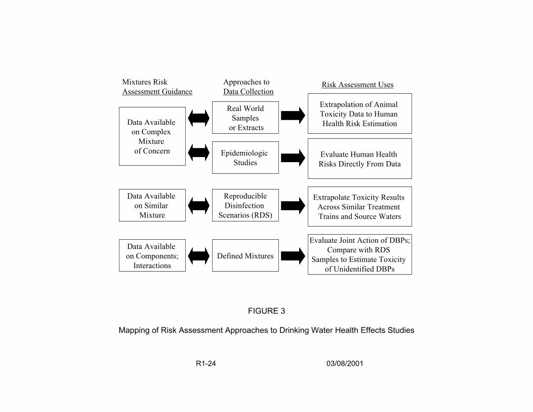
Mixtures Risk Assessment Guidance
Data Available on Complex
Mixture of Concern
Data Available on Similar
Mixture
Data Available on Components;
Interactions
Approaches to Data Collection
Real World Samples
or Extracts
Epidemiologic Studies
Reproducible Disinfection
Scenarios (RDS)
Defined Mixtures
FIGURE 3
Risk Assessment Uses
Extrapolation of Animal Toxicity Data to Human Health Risk Estimation
Evaluate Human Health Risks Directly From Data
Extrapolate Toxicity Results Across Similar Treatment Trains and Source Waters
Evaluate Joint Action of DBPs;Compare with RDS
Samples to Estimate Toxicity of Unidentified DBPs
Mapping of Risk Assessment Approaches to Drinking Water Health Effects Studies
R1-24 03/08/2001
advantages to testing the complex mixture of concern, this can also be problematic.
Toxicologic data from animal studies suffer from the uncertainties inherent in
extrapolation to human health risk. Epidemiologic data appear to be superior in terms
of evaluating humans directly, but these data suffer from confounding sources of
potential toxicity that can be difficult to account for.
The second approach uses data on a “sufficiently similar” mixture, represented
for DBPs by the toxicologic evaluation of Reproducible Disinfection Scenario (RDS)
samples (i.e., water samples produced by controlling the characteristics of source water
and then subjecting the samples to specific treatment trains). RDS samples may be
classified as similar mixtures with toxicity data that may provide a measure of the
expected toxicity of finished drinking water for a given treatment train and source water
characterization. Data in an RDS toxicity database could be judged for similarity against
data from a treatment plant by identifying and measuring the concentrations of DBPs in
each, comparing component proportions across the mixtures, and contrasting available
toxicity data on their components. For the RDS mixtures, the source of the mixtures is
controlled and measured so comparisons can be made across similar treatment trains
and source waters. Analytical chemistry is needed to characterize the composition and
stability of the mixtures. Toxicity data on the RDS samples are used to characterize
expected health effects. If the treatment plant data and the RDS mixture are judged to
be similar, then the quantitative risk assessment for the treatment process may be
derived from health effects data on the RDS sample.
Finally, the third mixtures risk assessment approach is to evaluate the DBP
mixture through an analysis of data on its components. This approach maps to the ILSI
R1-25 03/08/2001
panel’s testing of simple or “defined” mixtures of DBPs. For example, data from defined
mixture experiments (and also single chemical studies) could be used to perform a risk
assessment using a dose addition approach for DBPs thought to act by a similar mode-
of-action and or a response addition method for estimates of risk for DBPs thought to be
functionally independent. These particular procedures include a general assumption
that interaction effects at low concentration levels either do not occur at all or are small
enough to be insignificant to the risk characterization. Other, newer component-based
approaches that incorporate interactions information into the risk estimates when such
data are available are under development (Hertzberg et al., 1999; U.S. EPA, 1999c).
For DBPs, toxicity and concentration data on the components of a mixture can be
combined and added together (depending on the assumption used) to estimate
mixtures risk. Again, analytical chemistry is needed to identify and quantify the
components.
At least some data on DBPs exist for all these scenarios, so the method of risk
characterization chosen depends on the availability of health effects data, the
characterization of the exposure of interest, and the beliefs held relative to the toxicity of
the DBPs in the complex mixture, their interaction potential, and their likely mode(s)-of
action. Given all the data collection, evaluation and expert judgments that must be
performed, the risk assessor can then determine the most appropriate risk
characterization method to apply (U.S. EPA, 1999c).
The doses associated with human exposure to DBPs are all below the levels that
show adverse health effects when administered to animals, making extrapolation
necessary and the existence of a threshold effect level an important consideration. A
R1-26 03/08/2001
major concern is whether unidentified chemicals may produce “surprise” interactions,
even at low doses. Two major considerations in determining the likelihood of
toxicological interactions among DBP mixtures are that the DBPs are present at low
concentrations in drinking water and that a large number of compounds remain
unidentified.
Typically, little interaction is expected at the doses associated with exposure to
DBPs in drinking water. At the current, extremely low, environmental concentrations of
DBPs, synergistic toxicological interactions are not thought to occur. However, the
large number of uncharacterized compounds precludes completely ruling out the
possibility. An additional consideration that may result in possible interactions is
whether DBPs could accumulate in the body from constant exposure or whether there
could be an accumulation of impacts from exposure to hundreds of different chemicals,
each individually at a low level, but all acting (by the same mechanism or at different
steps in the same pharmacodynamic process) on some precursor stage leading to an
adverse health effect.
2.3. DBP EXPOSURES
The goal of an exposure assessment is to quantify the uptake of an agent or a
group of agents that results from an individual’s or a population’s contact with
environmental media (U.S. EPA, 1992; Paustenbauch, 2000). U.S. EPA (1992) defines
exposure assessment as the qualitative or quantitative “determination or estimation of
the magnitude, frequency, duration, and route of exposure.” Exposure assessments
involve three general steps:
R1-27 03/08/2001
• Estimation of the occurrence and concentrations of an agent or group of agents in various media that individuals contact
• Characterization of specific contact rates with the media
• Calculation of the likelihood of an exposure, the resulting uptake and biologically relevant dose rates, e.g., average daily exposure in terms of mg/kg/day, peak exposure, or cumulative exposure.
Exposures to DBP mixtures ultimately depend on concentrations of DBPs at the
tap (Olin, 1999). These concentrations at the tap depend upon fluxes in the DBP
concentrations within the distribution system. Very few consumers drink water directly
from a water treatment plant; most customers consume water that has passed through
a water distribution system. The concentration of the individual DBPs depends on the
water chemistry of the distributed water and the concentration and type of disinfectant.
The concentration of disinfectant also depends on the water chemistry and the
disinfectant demand associated with the distribution system. (For more details on
exposure data, see Sections 2.2., 3.4., 3.5., 3.6. of Report 2.) Water quality varies
throughout the distribution system because of changes taking place in the bulk phase of
the water and conditions existing at the interface between the bulk phase and the pipe
wall. To make exposure estimates more realistic, a series of dynamic models have
been developed to predict the concentrations of some individual DBPs at various times
in the distribution system (Clark, 1998; Clark and Sivaganesan, 1998).
Residence time in distribution systems affects DBP formation. In the United
States, distribution systems are frequently designed to ensure hydraulic reliability, which
includes adequate water quantity and pressure for fire flow as well as domestic and
industrial demand. To meet these goals, large amounts of storage are usually
R1-28 03/08/2001

incorporated into system design, resulting in long residence times, which in turn may
contribute to water quality deterioration.
Human exposure to DBPs is a classic complex exposure scenario (Olin, 1999).
DBP exposure patterns can be characterized as a multiple route, daily exposure to a
highly variable complex mixture of chemicals at low concentrations that inherently
reaches the general population, including sensitive subpopulations. DBPs have been
measured in tap water, vapors and aerosols. Some DBPs in tap water (e.g., chloroform)
volatilize through heating during cooking, showering, etc. (e.g., Weisel and Chen, 1994;
Giardino and Andelman, 1996). As a result, DBP exposures can occur through
ingestion, inhalation, and dermal absorption.
Mathematical exposure models have been developed for each exposure route;
several of these are summarized specifically for drinking water inhalation and dermal
exposures in Olin, 1999. Paustenbauch (2000) provides a general review of exposure
assessment and describes ingestion, inhalation and dermal exposure. The models
predict exposures based on such factors as the physical and chemical properties of
DBPs in water and assumptions concerning human activity patterns, as well as air
exchange rates in buildings and room dimensions (Olin, 1999). Studies of human
activity patterns in the U.S., such as tap water consumption distributions (including
heated tap water consumption), showering and bathing frequency and duration
distributions, provide contact rates for important exposure media (U.S. EPA, 1997b;
Johnson et al., 1999). These data can be aggregated and used in exposure modeling
to estimate DBP contact rates for the three primary exposure routes.
R1-29 03/08/2001
Mathematical models have been developed to estimate the absorbed doses from
oral, inhalation, and dermal routes. Absorbed dose is defined by the U.S. EPA (1997b)
as the amount crossing a specific absorption barrier through uptake processes. Report
2 describes an oral exposure model (Section 3.4.). In this model, DBP exposure is a
function of the concentration in water and the daily quantity of water ingested. Some
general models include a bioavailability parameter, although this was not included in this
modeling effort. The model used described a potential dose (i.e., the quantity ingested).
Both U.S. EPA (1994a) and Wilkes (1999), among others, describe inhalation exposure
models. Wilkes (1999) describes a model for estimating the absorbed dose of drinking
water contaminants including DBPs. The model estimates chemical exposures via
inhalation of aerosols and vapors. These may be generated from a number of
household uses including showers, clothes washers, dishwashers, and toilets. Bunge
and McDougal (1999) describe two broad classes of dermal penetration models:
membrane models and pharmacokinetic models. Both types of models can be used to
estimate absorbed doses. To estimate the absorbed dose of chloroform from drinking
water, Wilkes used an inhalation model and a membrane model for dermal exposure.
His results showed that the inhalation route is dominant for compounds that have a
higher volatility such as chloroform.
Further development of these models and extensions to DBP classes, such as
the HAAs and HANs, will be useful both to refine human exposure estimates and obtain
more relevant information from epidemiological studies (see Sections 4.1.1 and 4.8.1. of
Report 2). Difficulties in measuring both irregular exposure patterns and variable DBP
occurrence levels complicate interpretations of environmental epidemiological studies.
R1-30 03/08/2001
Some of the uncertainties have been discussed regarding the cancer literature (Murphy
et al., 1999; Poole and Greenland, 1999; U.S. EPA,1998b). Epidemiologic studies that
integrate more relevant exposure measures, data derived from mathematical models of
DBP exposures, and biomonitoring data are being developed. These improvements
may decrease many of the uncertainties in interpreting this literature in the near term.
In the longer term, DBP biomarkers may prove useful for refining exposure measures,
improving human dose-response assessment, and evaluating causality.
The development of quantitative measures of human exposure or effects from
exposure to DBPs from the three primary environmental exposure routes has proven to
be challenging. The development of biomarkers may aid the evaluation of these areas
of DBP research. Biomarkers are observable properties of an organism that can be
used to estimate prior exposure, to assess the underlying susceptibility of an organism,
and to identify changes or adverse effects resulting from exposures. Biomarkers can
occur at a number of functional levels within an organism: molecular, cellular, tissue, or
whole organism. Biomarker monitoring may provide a sensitive indicator of exposure,
susceptible subpopulations or individuals, or health. In the future, biomarkers offer the
potential advantage of integrating exposure and dose-response functions. The
development and use of these markers in human health risk assessment of
environmental chemicals are under active investigation. The following three areas of
biomarker research are being developed:
• Exposure biomarkers measure exogenous chemicals, metabolite(s) or the products of interactions with target molecules or cells in a compartment within an organism. This includes internal dosimeters of parent or metabolite concentrations and markers of biologically effective doses
R1-31 03/08/2001
• Susceptibility biomarkers indicate inherent or acquired properties of an organism that may lead to an increase in the internal dose or an increased level of the response resulting from exposure to a chemical or chemical class
• Effects biomarkers measure alterations of an organism that, depending on magnitude and nature, can indicate a potential or actual physical impairment or disease.
Some research efforts have focused on developing and evaluating biomarkers of
exposures to individual DBPs. Based on work described in Wallace et al. (1987) and
previous efforts in their laboratory, Weisel et al. (1999) evaluated two sets of exposure
biomarkers: 1) measuring the THM levels in exhaled breath; and 2) measuring the
urinary excretion rates and concentrations of dichloroacetic acid and trichloroacetic
acid. The rapid metabolism of THMs in the liver reduces body burden and breath
concentration following exposure; this rapid metabolism complicates the interpretation
of breath concentrations. Although both chloroform and bromodichloromethane
measurements taken immediately after shower exposures significantly correlated
statistically with concentrations in water, these measures and collection approaches still
need refinement before they can be used for purposes other than general markers of
inhalation and dermal exposure.
Pereira and Chang (1982) and Pereira et al. (1994) have developed blood
biomarkers that eventually may be useful in estimating the exposure to total THM, but
additional data are needed to describe the formation of adducts from individual THM
chemicals. THMs are metabolized to dihalocarbonyl, which binds cysteine. This bound
residue is metabolized, forming 2-oxothiazolidine-4-carboxylic acid, a urinary metabolite
of THM chemicals. Although measuring 2-hydroxythiazolidine-4-carboxy acid in
R1-32 03/08/2001
hemoglobin or albumin and the urinary excretion of 2-oxothiazolidine-4-carboxylic acid
would not distinguish individual THM chemicals from one another, it could serve as a
biomarker for total exposure to THMs. Data describing levels of the different THMs in
the drinking water and the rates at which each was metabolized could be used to
approximate the percentage of hemoglobin adduct produced by each THM.
A similar mechanism exists for the HANs. This may complicate attributing of a
given fraction of blood or urinary marker for THMs. Urinary dichloroacetic acid excretion
rates were not correlated to concentrations in drinking water; however, trichloroacetic
acid in the urine was a good marker of chronic exposure. Although these efforts are still
evolving, the use of biomarkers of exposure shows promise.
2.3.1. DBP Concentrations. A health risk assessment may consider many DBPs,
several hundred of which have been identified (Richardson, 1998). Chemicals
commonly found in finished drinking water are listed in Table 3. Figure 4 illustrates a
typical distribution of DBPs for a system that disinfects via a chlorination process,
including many of the DBPs listed in Table 3. Figure 4 also demonstrates the common
fact that more than 50% of the organic halogens produced by chlorination disinfection
are unidentified chemicals (62.4% in this instance). Similarly, less than 40% of the by-
products of ozonation have been identified (Weinberg, 1999). In general, these
unidentified DBPs include not only the organic halogens, but also non-halogenated
compounds in the water. Thus, the risk assessment must take into account that part of
the chemical exposure to humans that includes an unknown number of unidentified
chemicals likely to be found at extremely low concentrations.
R1-33 03/08/2001
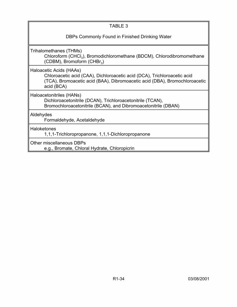
TABLE 3
DBPs Commonly Found in Finished Drinking Water
Trihalomethanes (THMs) Chloroform (CHCl3), Bromodichloromethane (BDCM), Chlorodibromomethane (CDBM), Bromoform (CHBr3)
Haloacetic Acids (HAAs) Chloroacetic acid (CAA), Dichloroacetic acid (DCA), Trichloroacetic acid (TCA), Bromoacetic acid (BAA), Dibromoacetic acid (DBA), Bromochloroacetic acid (BCA)
Haloacetonitriles (HANs) Dichloroacetonitrile (DCAN), Trichloroacetonitrile (TCAN), Bromochloroacetonitrile (BCAN), and Dibromoacetonitrile (DBAN)
Aldehydes Formaldehyde, Acetaldehyde
Haloketones 1,1,1-Trichloropropanone, 1,1,1-Dichloropropanone
Other miscellaneous DBPs e.g., Bromate, Chloral Hydrate, Chloropicrin
R1-34 03/08/2001
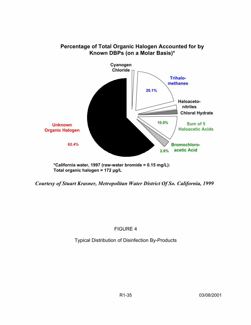
Percentage of Total Organic Halogen Accounted for by Known DBPs (on a Molar Basis)*
Cyanogen
Bromochloro-acetic Acid
Trihalomethanes
Chloride
20.1%
10.0%
2.8%
Haloaceto-nitriles
Chloral Hydrate
Unknown Sum of 5 Organic Halogen Haloacetic Acids
62.4%
*California water, 1997 (raw-water bromide = 0.15 mg/L): Total organic halogen = 172 µg/L
Courtesy of Stuart Krasner, Metropolitan Water District Of So. California, 1999
FIGURE 4
Typical Distribution of Disinfection By-Products
R1-35 03/08/2001

Assessing exposure to chemical mixtures of DBPs entails consideration of
several broad issues not encountered in single chemical risk assessments. First, when
assessing the current state of the analytic chemistry of DBPs, not only are the accuracy
and reliability of the measurement techniques critical, but also whether all of the
toxicologically relevant components have been identified (i.e., are there unidentified
components of the mixture?) or if the entire mixture has been measured at the points of
contact over time. Second, it should also be determined whether the key environmental
reactions have been identified and reaction rates measured. Important changes in the
concentrations of the DBP mixture components in the medium(a) of concern at the
point(s) of human contact must be identified (i.e., are all of the exposed individuals
receiving exposures to the same compounds, etc.). Finally, the bioavailability of the
mixture components must also be assessed. Important uncertainties must be identified
(and perhaps quantified): uncertainty based on imperfect analytic methods (e.g., some
constituents may not be characterized by the analytic technique that represents the
current state-of-the-science); extrapolations between concentrations at measurement
points and points of human exposure; unknown transformation reactions to the mixture
in the environment; and bioavailability. Each of these uncertainties in the risk
assessment must be discussed and accounted for in the final risk characterization.
2.3.2. Tap Water Exposure. Human exposure occurs only when an agent comes into
contact with the human membranes. For most individuals, DBPs primarily are
encountered indoors. The primary uses of indoor water are faucet use (drinking,
cooking, hand washing, etc), showering/bathing, toilet use, clothes washing and dish
washing (U.S. EPA, 1997b). DBPs may be present in liquid, vapor, or aerosol form(s),
R1-36 03/08/2001
can enter the body via ingestion, respiration, or dermal penetration, and may be
metabolized before distribution to the target organ(s).
The fate of DBPs in tap water depends on the water temperature and the nature
of use (Olin, 1999). For example, volatile DBPs are released when water is heated for
cooking and bathing; showering leads to increases in aerosolized DBPs; volatilization
and aerosolization of DBPs may be more limited during other water uses. The
concentrations of DBPs in the air also are dependent on the original concentrations in
the tap water, the volume of water used per activity, and structural characteristics (e.g.,
room dimensions, air flow patterns, etc.). For example, showering can utilize large
volumes of heated water.
For the oral route, DBP exposure can be estimated as a function of total tap
water consumed (L/kg-day), including all water from the household tap consumed
directly as a beverage or used to prepare foods and beverages. The studies of Ershow
and Cantor (1989) of the U.S. population and the Canadian Ministry of National Health
and Welfare (1981), presented in U.S. EPA (1997b) can be used to derive consumption
estimates. In addition, the Continuous Survey of Food Intake by Individuals (CSFII)
data (1994-1996) is currently undergoing evaluation within the EPA. Water
consumption data are also available for some subpopulations (e.g., pregnant women
(Ershow et al., 1991), persons with AIDs). Differences in DBP exposures occur
because of other factors, such as heated vs. unheated tap water or changes in
consumption patterns (e.g., in CSFII, increased use of bottled water).
Human activity patterns greatly influence DBP exposures via inhalation and
dermal routes. Human activity patterns including time spent at each activity as well as
R1-37 03/08/2001
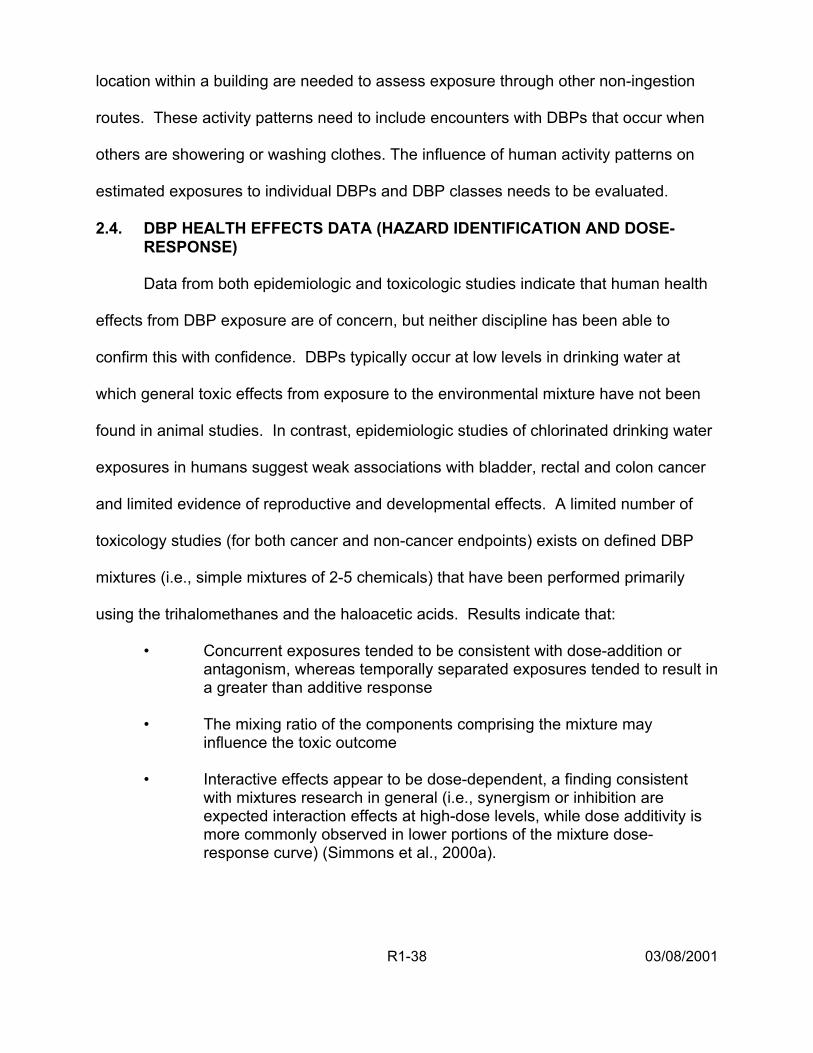
location within a building are needed to assess exposure through other non-ingestion
routes. These activity patterns need to include encounters with DBPs that occur when
others are showering or washing clothes. The influence of human activity patterns on
estimated exposures to individual DBPs and DBP classes needs to be evaluated.
2.4. DBP HEALTH EFFECTS DATA (HAZARD IDENTIFICATION AND DOSE-RESPONSE)
Data from both epidemiologic and toxicologic studies indicate that human health
effects from DBP exposure are of concern, but neither discipline has been able to
confirm this with confidence. DBPs typically occur at low levels in drinking water at
which general toxic effects from exposure to the environmental mixture have not been
found in animal studies. In contrast, epidemiologic studies of chlorinated drinking water
exposures in humans suggest weak associations with bladder, rectal and colon cancer
and limited evidence of reproductive and developmental effects. A limited number of
toxicology studies (for both cancer and non-cancer endpoints) exists on defined DBP
mixtures (i.e., simple mixtures of 2-5 chemicals) that have been performed primarily
using the trihalomethanes and the haloacetic acids. Results indicate that:
• Concurrent exposures tended to be consistent with dose-addition or antagonism, whereas temporally separated exposures tended to result in a greater than additive response
• The mixing ratio of the components comprising the mixture may influence the toxic outcome
• Interactive effects appear to be dose-dependent, a finding consistent with mixtures research in general (i.e., synergism or inhibition are expected interaction effects at high-dose levels, while dose additivity is more commonly observed in lower portions of the mixture dose-response curve) (Simmons et al., 2000a).
R1-38 03/08/2001
There is evidence in single chemical animal studies, at high DBP dose levels, of
carcinogenicity, reproductive effects, developmental effects, and other toxic effects,
particularly in the kidney and liver. Finally, there is evidence of mutagenicity and of
additivity using embryo cultures from exposure to extracts of finished drinking water in in
vitro studies.
2.4.1. Summary of Epidemiology Studies. Since the early 1970s, a large number of
epidemiologic studies of varying design and quality have been published in the scientific
literature. The studies have focused almost exclusively on chlorinated drinking water
and its association with cancer rather than on individual chemical exposures.
Reproductive and developmental epidemiologic studies on this topic first appeared in
the literature in the late 1980s. However, only recently have investigators collected
information to quantitatively estimate exposures to individuals from different chemical
families and species of DBPs and begun to study disinfectants other than chlorine. The
purpose of this section is to provide a brief overview of the existing epidemiologic
literature suggesting a potential hazard from exposure to disinfected drinking water and
its associated DBPs.
2.4.1.1. Cancer Studies — Several types of epidemiological studies have been
conducted to assess the association between cancer and chlorinated drinking water,
including ecological, cohort, and case-control designs, evaluating both incident and
decedent cancer cases. These studies differ in their basic approach and the evidence
they provide about the possible causality of an epidemiological association between
chlorinated drinking water and cancer. These studies are not reviewed in detail in this
document. However, a summary of the more methodologically sound studies (e.g.,
R1-39 03/08/2001
those based on incident cases that have interviews and some from of individual
exposure estimates) is provided in Table 4. The studies are described further in U.S.
EPA (1998a,b).
The results from these studies have not been used quantitatively for the current
risk assessment exercise because most of the exposure contrasts were confounded by
water source and none of the designs allowed for a comparison of the drinking water
treatment practices of interest to the current problem. In addition, recent research has
demonstrated evidence of publication bias, a form of selection bias, in the cancer
literature, where studies with inverse or null associations may not have been published
or submitted for publication by the investigators (Poole, 1997; Poole and Greenland,
1999; Murphy et al., 1999).
Based on the entire cancer-chlorinated drinking water epidemiology database,
there is better evidence for an association between exposure to chlorinated surface
water and bladder cancer than for other types of cancer. However, the latest bladder
cancer study (Cantor et al., 1998) notes several inconsistencies in results among the
studies for smokers/nonsmokers and males/females (Lang et al., 1998), and the
evidence is still considered insufficient to judge which water contaminants may be
important. Evidence for a role of THMs is weak at this time. A possible explanation for
the apparent discrepancies in findings for smokers and never-smokers among studies
may reside in water quality and water treatment differences in the respective study
areas, with resulting variations in the chemical composition of by-product mixtures.
R1-40 03/08/2001
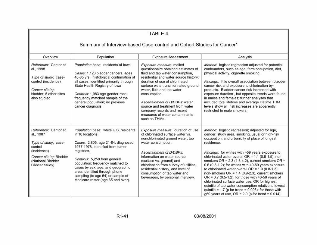
TABLE 4
Summary of Interview-based Case-control and Cohort Studies for Cancer*
Overview Population Exposure Assessment Analysis
Reference: Cantor et al., 1998 Type of study: case-control (incidence) Cancer site(s): bladder; 5 other sites also studied
Population base: residents of Iowa. Cases: 1,123 bladder cancers, ages 40-85 yrs., histological confirmation of all cases, identified primarily through State Health Registry of Iowa Controls: 1,983 age-gender-race frequency matched sample of the general population; no previous cancer diagnosis
Exposure measure: mailed questionnaire obtained estimates of fluid and tap water consumption, residential and water source history; duration of use of chlorinated surface water, unchlorinated ground water, fluid and tap water consumption. Ascertainment of D/DBPs: water source and treatment from water company records and recent measures of water contaminants such as THMs.
Method: logistic regression adjusted for potential confounders, such as age, farm occupation, diet, physical activity, cigarette smoking. Findings: little overall association between bladder cancer risk and exposure to chlorination by-products. Bladder cancer risk increased with exposure duration , but opposite trends were found in males and females; further analyses that included total lifetime and average lifetime THM levels show all risk increases are apparently restricted to male smokers.
Reference: Cantor et al., 1987 Type of study: case-control (incidence) Cancer site(s): Bladder (National Bladder Cancer Study)
Population base: white U.S. residents in 10 locations. Cases: 2,805, age 21-84, diagnosed 1977-1978, identified from tumor registries. Controls: 5,258 from general population; frequency matched to cases by sex, age, and geographic area; identified through phone sampling (to age 64) or sample of Medicare roster (age 65 and over).
Exposure measure: duration of use of chlorinated surface water vs. nonchlorinated ground water; tap water consumption. Ascertainment of D/DBPs: information on water source (surface vs. ground) and chlorination from survey of utilities; residential history, and level of consumption of tap water and beverages, by personal interview.
Method: logistic regression; adjusted for age, gender, study area, smoking, usual or high-risk occupation, and urbanicity of place of longest residence. Findings: for whites with >59 years exposure to chlorinated water overall OR = 1.1 (0.8-1.5), non-smokers OR = 2.3 (1.3-4.2), current smokers OR = 0.6 (0.3-1.2); for whites with 40-59 years exposure to chlorinated water overall OR = 1.0 (0.8-1.3), non-smokers OR = 1.4 (0.9-2.3), current smokers OR = 0.7 (0.5-1.2); for those with 40-59 years of chlorinated surface water use, OR for highest quintile of tap water consumption relative to lowest quintile = 1.7 (p for trend = 0.006); for those with >60 years of use, OR = 2.0 (p for trend = 0.014).
R1-41 03/08/2001
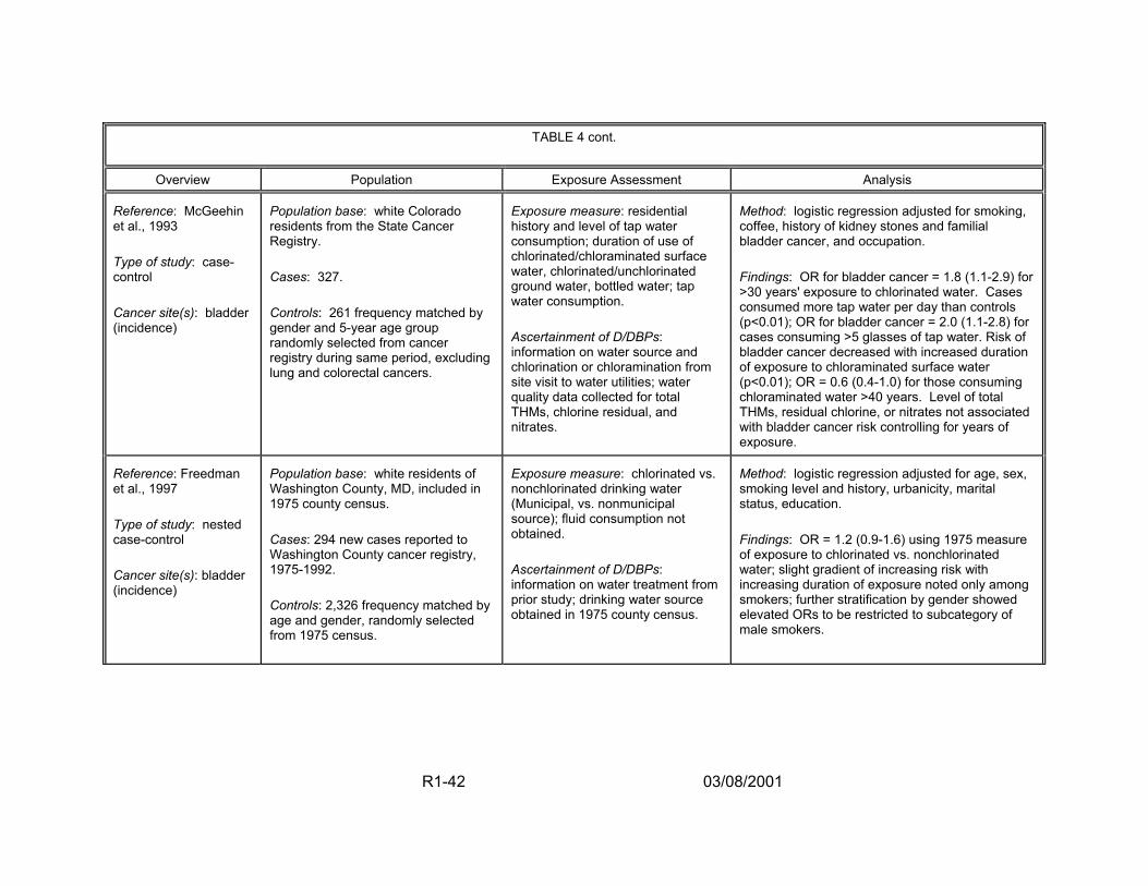
TABLE 4 cont.
Overview Population Exposure Assessment Analysis
Reference: McGeehin et al., 1993 Type of study: case-control Cancer site(s): bladder (incidence)
Population base: white Colorado residents from the State Cancer Registry. Cases: 327. Controls: 261 frequency matched by gender and 5-year age group randomly selected from cancer registry during same period, excluding lung and colorectal cancers.
Exposure measure: residential history and level of tap water consumption; duration of use of chlorinated/chloraminated surface water, chlorinated/unchlorinated ground water, bottled water; tap water consumption. Ascertainment of D/DBPs: information on water source and chlorination or chloramination from site visit to water utilities; water quality data collected for total THMs, chlorine residual, and nitrates.
Method: logistic regression adjusted for smoking, coffee, history of kidney stones and familial bladder cancer, and occupation. Findings: OR for bladder cancer = 1.8 (1.1-2.9) for >30 years' exposure to chlorinated water. Cases consumed more tap water per day than controls (p<0.01); OR for bladder cancer = 2.0 (1.1-2.8) for cases consuming >5 glasses of tap water. Risk of bladder cancer decreased with increased duration of exposure to chloraminated surface water (p<0.01); OR = 0.6 (0.4-1.0) for those consuming chloraminated water >40 years. Level of total THMs, residual chlorine, or nitrates not associated with bladder cancer risk controlling for years of exposure.
Reference: Freedman et al., 1997 Type of study: nested case-control Cancer site(s): bladder (incidence)
Population base: white residents of Washington County, MD, included in 1975 county census. Cases: 294 new cases reported to Washington County cancer registry, 1975-1992. Controls: 2,326 frequency matched by age and gender, randomly selected from 1975 census.
Exposure measure: chlorinated vs. nonchlorinated drinking water (Municipal, vs. nonmunicipal source); fluid consumption not obtained. Ascertainment of D/DBPs: information on water treatment from prior study; drinking water source obtained in 1975 county census.
Method: logistic regression adjusted for age, sex, smoking level and history, urbanicity, marital status, education. Findings: OR = 1.2 (0.9-1.6) using 1975 measure of exposure to chlorinated vs. nonchlorinated water; slight gradient of increasing risk with increasing duration of exposure noted only among smokers; further stratification by gender showed elevated ORs to be restricted to subcategory of male smokers.
R1-42 03/08/2001
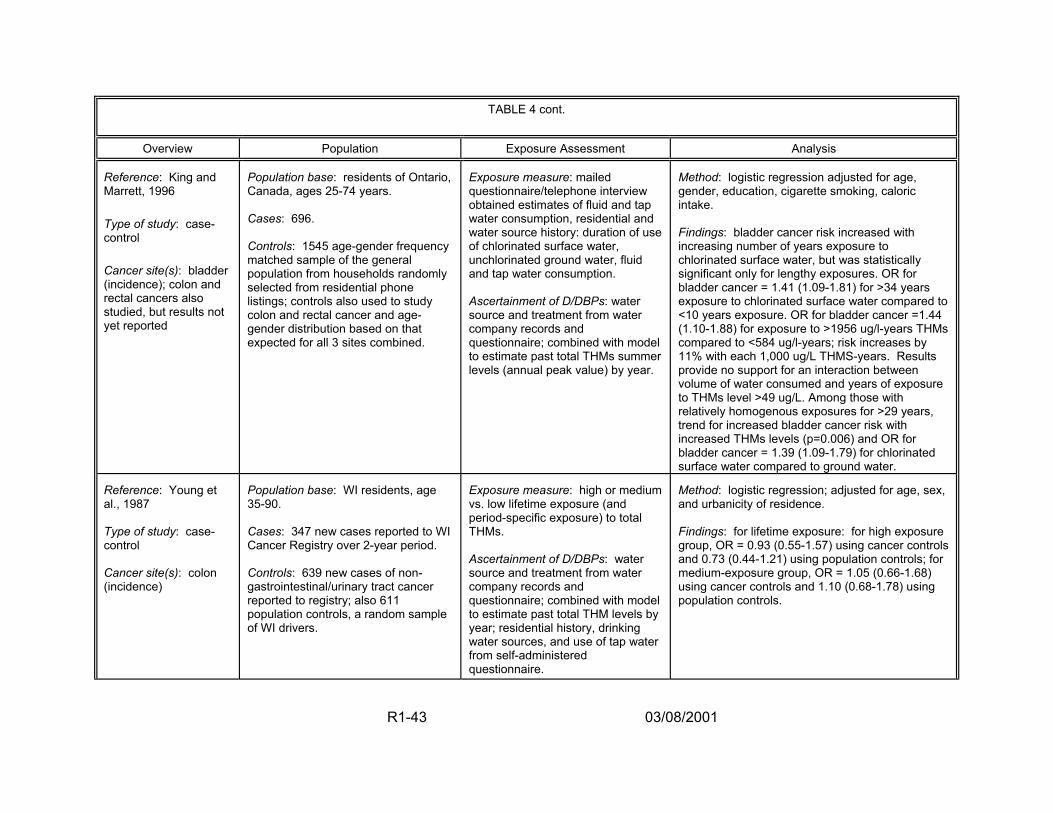
TABLE 4 cont.
Overview Population Exposure Assessment Analysis
Reference: King and Marrett, 1996 Type of study: case-control Cancer site(s): bladder (incidence); colon and rectal cancers also studied, but results not yet reported
Population base: residents of Ontario, Canada, ages 25-74 years. Cases: 696. Controls: 1545 age-gender frequency matched sample of the general population from households randomly selected from residential phone listings; controls also used to study colon and rectal cancer and age-gender distribution based on that expected for all 3 sites combined.
Exposure measure: mailed questionnaire/telephone interview obtained estimates of fluid and tap water consumption, residential and water source history: duration of use of chlorinated surface water, unchlorinated ground water, fluid and tap water consumption. Ascertainment of D/DBPs: water source and treatment from water company records and questionnaire; combined with model to estimate past total THMs summer levels (annual peak value) by year.
Method: logistic regression adjusted for age, gender, education, cigarette smoking, caloric intake. Findings: bladder cancer risk increased with increasing number of years exposure to chlorinated surface water, but was statistically significant only for lengthy exposures. OR for bladder cancer = 1.41 (1.09-1.81) for >34 years exposure to chlorinated surface water compared to <10 years exposure. OR for bladder cancer =1.44 (1.10-1.88) for exposure to >1956 ug/l-years THMs compared to <584 ug/l-years; risk increases by 11% with each 1,000 ug/L THMS-years. Results provide no support for an interaction between volume of water consumed and years of exposure to THMs level >49 ug/L. Among those with relatively homogenous exposures for >29 years, trend for increased bladder cancer risk with increased THMs levels (p=0.006) and OR for bladder cancer = 1.39 (1.09-1.79) for chlorinated surface water compared to ground water.
Reference: Young et al., 1987 Type of study: case-control Cancer site(s): colon (incidence)
Population base: WI residents, age 35-90. Cases: 347 new cases reported to WI Cancer Registry over 2-year period. Controls: 639 new cases of non-gastrointestinal/urinary tract cancer reported to registry; also 611 population controls, a random sample of WI drivers.
Exposure measure: high or medium vs. low lifetime exposure (and period-specific exposure) to total THMs. Ascertainment of D/DBPs: water source and treatment from water company records and questionnaire; combined with model to estimate past total THM levels by year; residential history, drinking water sources, and use of tap water from self-administered questionnaire.
Method: logistic regression; adjusted for age, sex, and urbanicity of residence. Findings: for lifetime exposure: for high exposure group, OR = 0.93 (0.55-1.57) using cancer controls and 0.73 (0.44-1.21) using population controls; for medium-exposure group, OR = 1.05 (0.66-1.68) using cancer controls and 1.10 (0.68-1.78) using population controls.
R1-43 03/08/2001
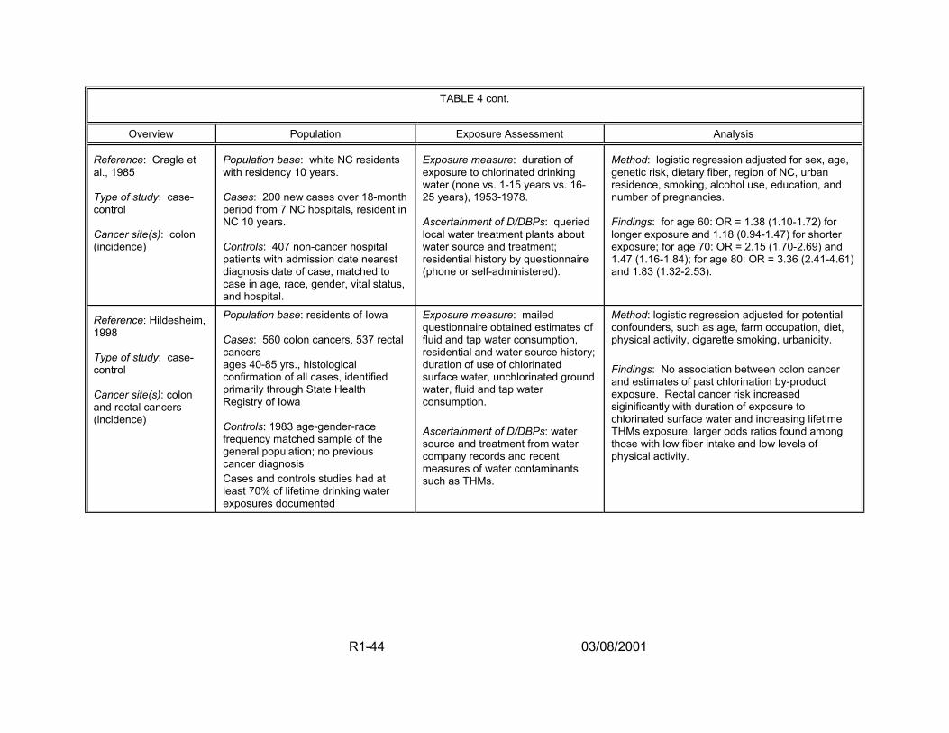
TABLE 4 cont.
Overview Population Exposure Assessment Analysis
Reference: Cragle et al., 1985 Type of study: case-control Cancer site(s): colon (incidence)
Population base: white NC residents with residency 10 years. Cases: 200 new cases over 18-month period from 7 NC hospitals, resident in NC 10 years. Controls: 407 non-cancer hospital patients with admission date nearest diagnosis date of case, matched to case in age, race, gender, vital status, and hospital.
Exposure measure: duration of exposure to chlorinated drinking water (none vs. 1-15 years vs. 16-25 years), 1953-1978. Ascertainment of D/DBPs: queried local water treatment plants about water source and treatment; residential history by questionnaire (phone or self-administered).
Method: logistic regression adjusted for sex, age, genetic risk, dietary fiber, region of NC, urban residence, smoking, alcohol use, education, and number of pregnancies. Findings: for age 60: OR = 1.38 (1.10-1.72) for longer exposure and 1.18 (0.94-1.47) for shorter exposure; for age 70: OR = 2.15 (1.70-2.69) and 1.47 (1.16-1.84); for age 80: OR = 3.36 (2.41-4.61) and 1.83 (1.32-2.53).
Reference: Hildesheim, 1998 Type of study: case-control Cancer site(s): colon and rectal cancers (incidence)
Population base: residents of Iowa Cases: 560 colon cancers, 537 rectal cancers ages 40-85 yrs., histological confirmation of all cases, identified primarily through State Health Registry of Iowa Controls: 1983 age-gender-race frequency matched sample of the general population; no previous cancer diagnosis Cases and controls studies had at least 70% of lifetime drinking water exposures documented
Exposure measure: mailed questionnaire obtained estimates of fluid and tap water consumption, residential and water source history; duration of use of chlorinated surface water, unchlorinated ground water, fluid and tap water consumption. Ascertainment of D/DBPs: water source and treatment from water company records and recent measures of water contaminants such as THMs.
Method: logistic regression adjusted for potential confounders, such as age, farm occupation, diet, physical activity, cigarette smoking, urbanicity. Findings: No association between colon cancer and estimates of past chlorination by-product exposure. Rectal cancer risk increased siginificantly with duration of exposure to chlorinated surface water and increasing lifetime THMs exposure; larger odds ratios found among those with low fiber intake and low levels of physical activity.
R1-44 03/08/2001
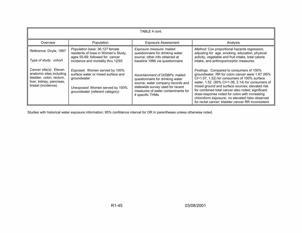
TABLE 4 cont.
Overview Population Exposure Assessment Analysis
Reference: Doyle, 1997 Type of study: cohort Cancer site(s): Eleven anatomic sites including bladder, colon, rectum, liver, kidney, pancreas, breast (incidence)
Population base: 36,127 female residents of Iowa in Women’s Study, ages 55-69; followed for cancer incidence and mortality thru 12/93 Exposed: Women served by 100% surface water or mixed surface and groundwater Unexposed: Women served by 100% groundwater (referent category)
Exposure measure: mailed questionnaire for drinking water source; other info obtained at baseline 1986 via questionnaire Ascertainment of D/DBPs: mailed questionnaire for drinking water source; water company records and statewide survey used for recent measures of water contaminants for 4 specific THMs
Method: Cox proportional hazards regression, adjusting for age, smoking, education, physical activity, vegetable and fruit intake, total calorie intake, and anthropomorphic measures. Findings: Compared to consumers of 100% groundwater, RR for colon cancer were 1.67 (95% CI=1.07, 1.52) for consumers of 100% surface water, 1.52 (95% CI=1.08, 2.14) for consumers of mixed ground and surface sources; elevated risk for combined total cancer also noted; significant dose-response noted for colon with increasing chloroform exposure; no elevated risks observed for rectal cancer; bladder cancer RR inconsistent.
Studies with historical water exposure information; 95% confidence interval for OR in parentheses unless otherwise noted.
R1-45 03/08/2001
This continues to reinforce the need for better exposure assessments in this literature to
reduce the possibility of missing a true risk because it has been diluted by
nondifferential exposure misclassification.
Expert evaluations over the past 20 years of the epidemiological data for
chlorinated drinking water/DBPs and cancer have been made by the National Academy
of Science (NAS), International Association for Research on Cancer (IARC), EPA,
International Society for Environmental Epidemiology (ISEE), International Life Sciences
Institute (ILSI), Health Canada, and the World Health Organization International
Programme on Chemical Substance (WHO-IPCS) among others. In general, the
consensus is that the data have limitations and that a conclusion as to a causal
relationship cannot be drawn (IARC, 1991; Neutra and Ostro, 1992; Craun et al. 1993;
U.S. EPA, 1994b, 1997c; Reif et al., 1996; Mills et al., 1998).
To improve this body of literature, EPA has an ongoing project to acquire more
complete chemical occurrence and water quality data that can be used to develop
models for predicting the historic levels of THM occurrence (and in some cases,
haloacetic acids) in specific geographic areas where epidemiologic studies have been
performed, e.g., Iowa and Ontario, Canada (Murphy et al., 2000). The models,
developed with historical data from water utilities, will be used to re-evaluate the
exposure assessment component of certain recently completed studies, which will then
be appropriately reanalyzed. This research should help reduce some of the
uncertainties and problems outlined above, particularly the need for valid,
R1-46 03/08/2001
unconfounded exposure measures that can separate effects of water source from the
DBPs and other chemical constituents in the water source.
2.4.1.2. Reproductive and Developmental Studies — Although fewer in
number than the body of cancer literature, epidemiological studies of reproductive and
developmental outcomes also have been performed. The outcomes considered have
included stillbirth, spontaneous abortion, low birth weight, intrauterine growth
retardation, somatic effects, and various birth defects including cardiac and neural tube
defects. Almost all of these studies examined multiple outcomes and multiple exposure
variables and most have used different operational definitions for study endpoints and
exposures. A summary of this literature is given in Table 5 and a more detailed
description can be found in U.S. EPA (1998a).
In 1993, an expert scientific panel convened by EPA and ILSI (ILSI, 1993; Reif et
al., 1996) reviewed the epidemiologic literature on reproductive and developmental
endpoints and DBP and disinfectant exposures. They concluded that the research in
this area was in a very early and evolving stage and that the studies should be viewed
as preliminary. A second expert panel convened by EPA in 1997 reviewed more
recently completed studies and reached a similar conclusion. Although several studies
have suggested that increased risks of neural tube defects and miscarriage may be
associated with THMs or selected THM species, additional studies are needed to
determine whether the observed associations are causal. The epidemiologic literature
on adverse reproductive and developmental outcomes is still very sparse and must
R1-47 03/08/2001
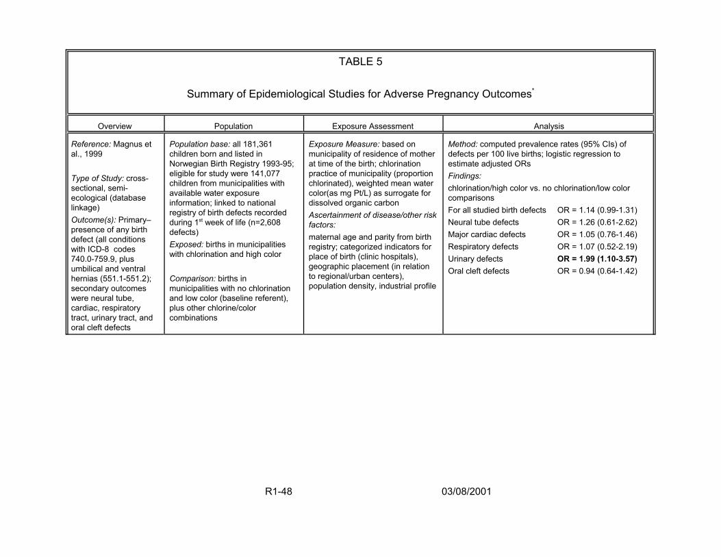
TABLE 5
Summary of Epidemiological Studies for Adverse Pregnancy Outcomes*
Overview Population Exposure Assessment Analysis
Reference: Magnus et al., 1999
Type of Study: cross-sectional, semi-ecological (database linkage) Outcome(s): Primary– presence of any birth defect (all conditions with ICD-8 codes 740.0-759.9, plus umbilical and ventral hernias (551.1-551.2); secondary outcomes were neural tube, cardiac, respiratory tract, urinary tract, and oral cleft defects
Population base: all 181,361 children born and listed in Norwegian Birth Registry 1993-95; eligible for study were 141,077 children from municipalities with available water exposure information; linked to national registry of birth defects recorded during 1st week of life (n=2,608 defects) Exposed: births in municipalities with chlorination and high color
Comparison: births in municipalities with no chlorination and low color (baseline referent), plus other chlorine/color combinations
Exposure Measure: based on municipality of residence of mother at time of the birth; chlorination practice of municipality (proportion chlorinated), weighted mean water color(as mg Pt/L) as surrogate for dissolved organic carbon Ascertainment of disease/other risk factors: maternal age and parity from birth registry; categorized indicators for place of birth (clinic hospitals), geographic placement (in relation to regional/urban centers), population density, industrial profile
Method: computed prevalence rates (95% CIs) of defects per 100 live births; logistic regression to estimate adjusted ORs Findings: chlorination/high color vs. no chlorination/low color comparisons For all studied birth defects OR = 1.14 (0.99-1.31) Neural tube defects OR = 1.26 (0.61-2.62) Major cardiac defects OR = 1.05 (0.76-1.46) Respiratory defects OR = 1.07 (0.52-2.19) Urinary defects OR = 1.99 (1.10-3.57) Oral cleft defects OR = 0.94 (0.64-1.42)
R1-48 03/08/2001

TABLE 5 cont.
Overview Population Exposure Assessment Analysis
Reference: Klotz and Pyrch, 1999
Type of Study: population-based case-control
Outcome(s): neural tube defects
(NTDs)
Population base: all New Jersey births 1993-1994;
Cases: 112 neural tube defects ascertained through NJ Birth Defects Registry and Fetal Death Registry (n=76 spina bifida only, 19 anencephaly only, 8 encephalocele only, 9 combination defects)
Controls: 248 randomly selected from all NJ births; term births <2,500 g and infants with other defects excluded
Exposure Measure: estimated on basis of mother’s residence at time of neural tube closure (1st month of gestation), using water utility data for individual & THMs; post-birth in-home water sample collection for THMs, total and free chlorine, haloacetonitriles (HANs), haloacetic acids (HAAs) timed to coincide with critical window 1 yr. earlier. Ascertainment of disease/other risk factors: Birth certificates plus interviews, interviewers blinded to exposure status of participants; pregnancy & medical history, parental occupation; behaviors & exposures for 3 mo. before & 1 mo. after conception including tap water ingestion, showering, bathing, swimming; use of water filters and vitamin use.
Method: prevalence ORs calculated with logistic regression; exposure categories based on prior studies
Findings: For subjects with known residency at conception– public monitoring data concurrent w/ 1st month of pregnancy: surface vs. ground source OR = 1.6 (0.9 - 2.8) TTHMs (ppb) 40+ vs. <5 OR = 1.7 (1.0 - 3.1) in-home tap water sample 1 yr after 1st month of pregnancy: surface vs. ground source OR = 1.7 (0.8 - 3.6) TTHMs (ppb) 40+ vs. <5 OR = 2.0 (0.9 - 4.9) No association with total tap water or cold tap water ingested, irrespective of THM levels; HAAs (ppb) 35+ vs. <3 OR = 1.2 (0.5 - 2.6) HANs (ppb) 3.0+ vs. <0.5 OR = 1.3 (0.6 - 2.5)
R1-49 03/08/2001
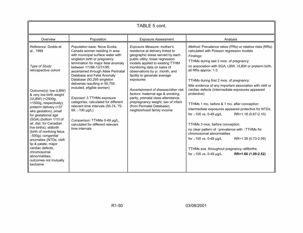
TABLE 5 cont.
Overview Population Exposure Assessment Analysis
Reference: Dodds et al., 1999
Type of Study: retrospective cohort
Outcome(s): low (LBW) & very low birth weight (VLBW) (<2500g, <1500g, respectively); preterm delivery (<37 wks gestation); small for gestational age (SGA) (bottom 1/10 of wt. dist. for Canadian live births); stillbirth (birth of nonliving fetus $500g); congenital anomalies (NTDs, cleft lip & palate, major cardiac defects, chromosomal abnormalities; outcomes not mutually exclusive
Population base: Nova Scotia, Canada women residing in area with municipal surface water with singleton birth or pregnancy termination for major fetal anomaly between 1/1/88-12/31/95, ascertained through Atlee Perinatal Database and Fetal Anomaly Database (93,295 singleton deliveries resulting in 50,755 included, eligible women)
Exposed: 3 TTHMs exposure categories, calculated for different relevant time intervals (50-74, 75-99, $100 µg/L)
Comparison: TTHMs 0-49 µg/L, calculated for different relevant time intervals
Exposure Measure: mother’s residence at delivery linked to geographic areas served by each public utility; linear regression models applied to existing TTHM monitoring data on basis of observations by yr, month, and facility to generate average exposures
Ascertainment of disease/other risk factors: maternal age & smoking, parity, prenatal class attendance, prepregnancy weight, sex of infant (from Perinatal Database); neighborhood family income
Method: Prevalence ratios (PRs) or relative risks (RRs) calculated with Poisson regression models Findings: TTHMs during last 3 mos. of pregnancy: no association with SGA, LBW, VLBW or preterm birth, all RRs approx. 1.0
TTHMs during first 2 mos. of pregnancy: little evidence of any important association with cleft or cardiac defects (intermediate exposures appeared protective)
TTHMs 1 mo. before & 1 mo. after conception: intermediate exposures appeared protective for NTDs; for $100 vs. 0-49 µg/L RR=1.18 (0.67-2.10)
TTHMs 3 mos. before conception: no clear pattern of 8prevalence with 8TTHMs for chromosomal abnormalities for $100 vs. 0-49 µg/L RR=1.38 (0.73-2.59)
TTHMs ave. throughout pregnancy–stillbirths for $100 vs. 0-49 µg/L RR=1.66 (1.09-2.52)
R1-50 03/08/2001
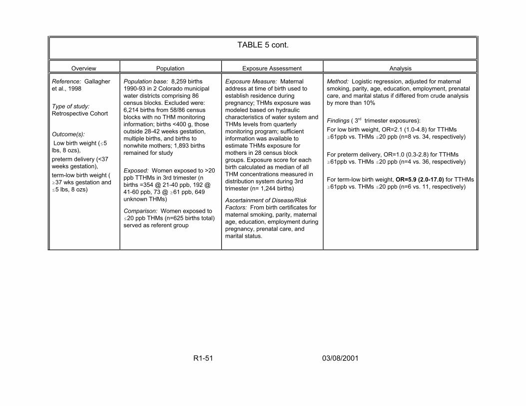
TABLE 5 cont.
Overview Population Exposure Assessment Analysis
Reference: Gallagher et al., 1998
Type of study: Retrospective Cohort
Outcome(s): Low birth weight (#5
lbs, 8 ozs), preterm delivery (<37 weeks gestation), term-low birth weight ( $37 wks gestation and #5 lbs, 8 ozs)
Population base: 8,259 births 1990-93 in 2 Colorado municipal water districts comprising 86 census blocks. Excluded were: 6,214 births from 58/86 census blocks with no THM monitoring information; births <400 g, those outside 28-42 weeks gestation, multiple births, and births to nonwhite mothers; 1,893 births remained for study
Exposed: Women exposed to >20 ppb TTHMs in 3rd trimester (n births =354 @ 21-40 ppb, 192 @ 41-60 ppb, 73 @ $61 ppb, 649 unknown THMs)
Comparison: Women exposed to #20 ppb THMs (n=625 births total) served as referent group
Exposure Measure: Maternal address at time of birth used to establish residence during pregnancy; THMs exposure was modeled based on hydraulic characteristics of water system and THMs levels from quarterly monitoring program; sufficient information was available to estimate THMs exposure for mothers in 28 census block groups. Exposure score for each birth calculated as median of all THM concentrations measured in distribution system during 3rd trimester (n= 1,244 births)
Ascertainment of Disease/Risk Factors: From birth certificates for maternal smoking, parity, maternal age, education, employment during pregnancy, prenatal care, and marital status.
Method: Logistic regression, adjusted for maternal smoking, parity, age, education, employment, prenatal care, and marital status if differed from crude analysis by more than 10%
Findings ( 3rd trimester exposures): For low birth weight, OR=2.1 (1.0-4.8) for TTHMs $61ppb vs. THMs #20 ppb (n=8 vs. 34, respectively)
For preterm delivery, OR=1.0 (0.3-2.8) for TTHMs $61ppb vs. THMs #20 ppb (n=4 vs. 36, respectively)
For term-low birth weight, OR=5.9 (2.0-17.0) for TTHMs $61ppb vs. THMs #20 ppb (n=6 vs. 11, respectively)
R1-51 03/08/2001
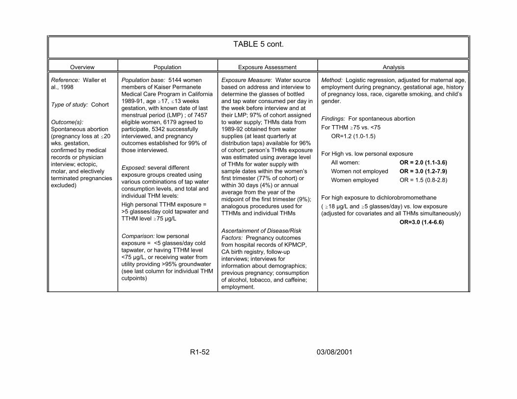
TABLE 5 cont.
Overview Population Exposure Assessment Analysis
Reference: Waller et al., 1998
Type of study: Cohort
Outcome(s): Spontaneous abortion (pregnancy loss at #20 wks. gestation, confirmed by medical records or physician interview; ectopic, molar, and electively terminated pregnancies excluded)
Population base: 5144 women members of Kaiser Permanete Medical Care Program in California 1989-91, age $17, #13 weeks gestation, with known date of last menstrual period (LMP) ; of 7457 eligible women, 6179 agreed to participate, 5342 successfully interviewed, and pregnancy outcomes established for 99% of those interviewed.
Exposed: several different exposure groups created using various combinations of tap water consumption levels, and total and individual THM levels: High personal TTHM exposure = >5 glasses/day cold tapwater and TTHM level $75 µg/L
Comparison: low personal exposure = <5 glasses/day cold tapwater, or having TTHM level <75 µg/L, or receiving water from utility providing >95% groundwater (see last column for individual THM cutpoints)
Exposure Measure: Water source based on address and interview to determine the glasses of bottled and tap water consumed per day in the week before interview and at their LMP; 97% of cohort assigned to water supply; THMs data from 1989-92 obtained from water supplies (at least quarterly at distribution taps) available for 96% of cohort; person’s THMs exposure was estimated using average level of THMs for water supply with sample dates within the women’s first trimester (77% of cohort) or within 30 days (4%) or annual average from the year of the midpoint of the first trimester (9%); analogous procedures used for TTHMs and individual THMs
Ascertainment of Disease/Risk Factors: Pregnancy outcomes from hospital records of KPMCP, CA birth registry, follow-up interviews; interviews for information about demographics; previous pregnancy; consumption of alcohol, tobacco, and caffeine; employment.
Method: Logistic regression, adjusted for maternal age, employment during pregnancy, gestational age, history of pregnancy loss, race, cigarette smoking, and child’s gender.
Findings: For spontaneous abortion For TTHM $75 vs. <75
OR=1.2 (1.0-1.5)
For High vs. low personal exposure All women: OR = 2.0 (1.1-3.6) Women not employed OR = 3.0 (1.2-7.9) Women employed OR = 1.5 (0.8-2.8)
For high exposure to dichlorobromomethane ( $18 µg/L and $5 glasses/day) vs. low exposure (adjusted for covariates and all THMs simultaneously)
OR=3.0 (1.4-6.6)
R1-52 03/08/2001
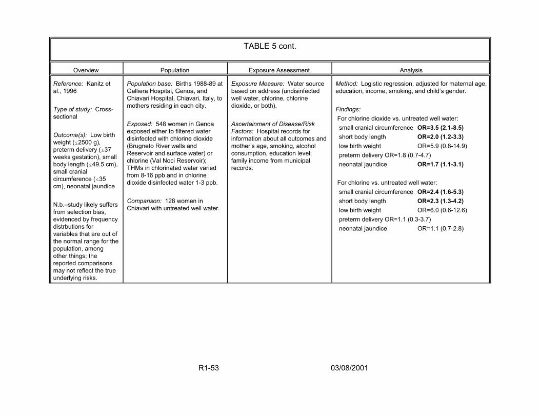
TABLE 5 cont.
Overview Population Exposure Assessment Analysis
Reference: Kanitz et al., 1996
Type of study: Cross-sectional
Outcome(s): Low birth weight (#2500 g), preterm delivery (#37 weeks gestation), small body length (#49.5 cm), small cranial circumference (#35 cm), neonatal jaundice
N.b.–study likely suffers from selection bias, evidenced by frequency distrbutions for variables that are out of the normal range for the population, among other things; the reported comparisons may not reflect the true underlying risks.
Population base: Births 1988-89 at Galliera Hospital, Genoa, and Chiavari Hospital, Chiavari, Italy, to mothers residing in each city.
Exposed: 548 women in Genoa exposed either to filtered water disinfected with chlorine dioxide (Brugneto River wells and Reservoir and surface water) or chlorine (Val Noci Reservoir); THMs in chlorinated water varied from 8-16 ppb and in chlorine dioxide disinfected water 1-3 ppb.
Comparison: 128 women in Chiavari with untreated well water.
Exposure Measure: Water source based on address (undisinfected well water, chlorine, chlorine dioxide, or both).
Ascertainment of Disease/Risk Factors: Hospital records for information about all outcomes and mother’s age, smoking, alcohol consumption, education level; family income from municipal records.
Method: Logistic regression, adjusted for maternal age, education, income, smoking, and child’s gender.
Findings: For chlorine dioxide vs. untreated well water: small cranial circumference OR=3.5 (2.1-8.5) short body length OR=2.0 (1.2-3.3) low birth weight OR=5.9 (0.8-14.9) preterm delivery OR=1.8 (0.7-4.7) neonatal jaundice OR=1.7 (1.1-3.1)
For chlorine vs. untreated well water: small cranial circumference OR=2.4 (1.6-5.3) short body length OR=2.3 (1.3-4.2) low birth weight OR=6.0 (0.6-12.6) preterm delivery OR=1.1 (0.3-3.7) neonatal jaundice OR=1.1 (0.7-2.8)
R1-53 03/08/2001
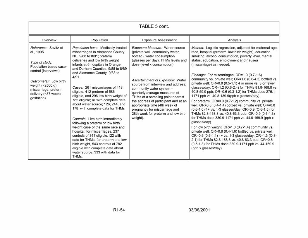
TABLE 5 cont.
Overview Population Exposure Assessment Analysis
Reference: Savitz et al., 1995
Type of study: Population based case-control (interviews)
Outcome(s): Low birth weight (<2500 g), miscarriage, preterm delivery (<37 weeks gestation)
Population base: Medically treated miscarriages in Alamance County, NC, 9/88 to 8/91; preterm deliveries and low birth weight infants at 6 hospitals in Orange and Durham Counties, 9/88 to 8/89 and Alamance County, 9/88 to 4/91.
Cases: 261 miscarriages of 418 eligible, 412 preterm of 586 eligible, and 296 low birth weight of 782 eligible; all with complete data about water source; 126, 244, and 178 with complete data for THMs
Controls: Live birth immediately following a preterm or low birth weight case of the same race and hospital; for miscarriages, 237 controls of 341 eligible,122 with data for THMs; for preterm and low birth weight, 543 controls of 782 eligible with complete data about water source, 333 with data for THMs.
Exposure Measure: Water source (private well, community water, bottled); water consumption (glasses per day); THMs levels and dose (level x consumption)
Ascertainment of Exposure: Water source from interview and address; community water system – quarterly average measures of THMs at a sampling point nearest the address of participant and at an appropriate time (4th week of pregnancy for miscarriage and 28th week for preterm and low birth weight).
Method: Logistic regression, adjusted for maternal age, race, hospital (preterm, low birth weight), education, smoking, alcohol consumption, poverty level, marital status, education, employment and nausea (miscarriage) as needed.
Findings: For miscarriages, OR=1.0 (0.7-1.6) community vs. private well; OR=1.6 (0.6-4.3) bottled vs. private well; OR=0.8 (0.5-1.1) 4 or more vs. 3 or fewer glasses/day; OR=1.2 (O.6-2.4) for THMs 81.8-168.8 vs. 40.8-59.9 ppb; OR=0.6 (0.3-1.2) for THMs dose 275.1-1171 ppb vs. 40.8-139.9(ppb x glasses/day). For preterm, OR=0.9 (0.7-1.2) community vs. private well; OR=0.8 (0.4-1.4) bottled vs. private well; OR=0.8 (0.6-1.0) 4+ vs. 1-3 glasses/day; OR=0.9 (O.6-1.5) for THMs 82.8-168.8 vs. 40.8-63.3 ppb; OR=0.9 (0.6-1.3) for THMs dose 330.9-1171 ppb vs. 44.0-169.9 (ppb x glasses/day). For low birth weight, OR=1.0 (0.7-1.4) community vs. private well; OR=0.8 (0.4-1.6) bottled vs. private well; OR=0.6 (0.6-1.1) 4+ vs. 1-3 glasses/day; OR=1.3 (O.8-2.1) for THMs 82.8-168.8 vs. 40.8-63.3 ppb; OR=0.8 (0.5-1.3) for THMs dose 330.9-1171 ppb vs. 44-169.9 (ppb x glasses/day).
R1-54 03/08/2001
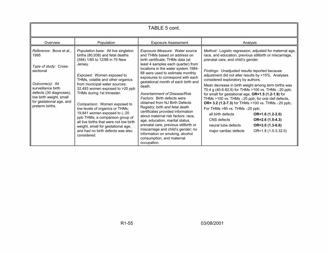
TABLE 5 cont.
Overview Population Exposure Assessment Analysis
Reference: Bove et al., 1995
Type of study: Cross-sectional
Outcome(s): All surveillance birth defects (30 diagnoses), low birth weight, small for gestational age, and preterm births.
Population base: All live singleton births (80,938) and fetal deaths (594) 1/85 to 12/88 in 75 New Jersey.
Exposed: Women exposed to THMs, volatile and other organics from municipal water sources; 32,493 women exposed to >20 ppb THMs during 1st trimester.
Comparison: Women exposed to low levels of organics or THMs; 19,841 women exposed to (#20 ppb THMs; a comparison group of all live births that were not low birth weight, small for gestational age, and had no birth defects was also considered.
Exposure Measure: Water source and THMs based on address on birth certificate; THMs data (at least 4 samples each quarter) from locations in the water system 1984-88 were used to estimate monthly exposures to correspond with each gestational month of each birth and death.
Ascertainment of Disease/Risk Factors: Birth defects were obtained from NJ Birth Defects Registry; birth and fetal death certificates provided information about maternal risk factors: race, age, education, marital status, prenatal care, previous stillbirth or miscarriage and child’s gender; no information on smoking, alcohol consumption, and maternal occupation.
Method: Logistic regression, adjusted for maternal age, race, and education, previous stillbirth or miscarriage, prenatal care, and child’s gender.
Findings: Unadjusted results reported because adjustment did not alter results by >15%. Analyses considered exploratory by authors. Mean decrease in birth weight among term births was 70.4 g (40.6-82.6) for THMs >100 vs. THMs #20 ppb; for small for gestational age, OR=1.5 (1.2-1.9) for THMs >100 vs. THMs #20 ppb; for oral clef defects, OR= 3.2 (1.2-7.3) for THMs >100 vs. THMs #20 ppb;. For THMs >80 vs. THMs #20 ppb:
all birth defects OR=1.6 (1.2-2.0) CNS defects OR=2.6 (1.5-4.3) neural tube defects OR=3.0 (1.3-6.6) major cardiac defects OR=1.8 (1.0-3.32.0)
R1-55 03/08/2001

TABLE 5 cont.
Overview Population Exposure Assessment Analysis
Reference: Aschengrau et al., 1993
Type of study: Nested case-control with interviews
Outcome(s): Congenital anomalies (live/stillborrn infant with 1 or more anomalies), stillbirths (without anomalies), and neonatal deaths (live-born infants without anomalies, dying within 1 week of birth)
Population base: Cohort of 14,130 obstetric patients who delivered from 8/77 to 3/80 at Boston Hospital for Women (83% of all delivery patients).
Cases: 1314 congenital anomalies; 121 stillbirths; 76 neonatal deaths (1039, 77, and 55 cases in study, respectively)
Controls: 1490 randomly selected women who delivered infants alive at discharge and without anomalies (1177 in study)
Exposure Measure: Water source (surface, ground, or mixed; chlorine or chloramine); and routine water analyses of minerals, metals, and other chemicals (no THMs); analyses closest to date of conception (median interval 3.3 months). Ascertainment of Exposure/Covariates: Address (at time of pregnancy outcome or 1st
trimester if available) used to assign water exposures; interview used to collect information about maternal habits and demographic characteristics.
Method: Logistic regression, adjusted for maternal age, race, hospital payment method, history of anomaly, alcohol consumption, and water source.
Findings: For chlorinated vs. chloraminated surface water Stillbirths OR = 2.6 (0.9-7.5) congenital anomalies, neonatal deaths OR-=1.0 (no reported CI) All major malformations OR = 1.5 (0.7-2.1)
Respiratory defects OR = 3.2 (1.1-9.5) Urinary tract defects OR = 4.1 (1.2 -14.1)
R1-56 03/08/2001
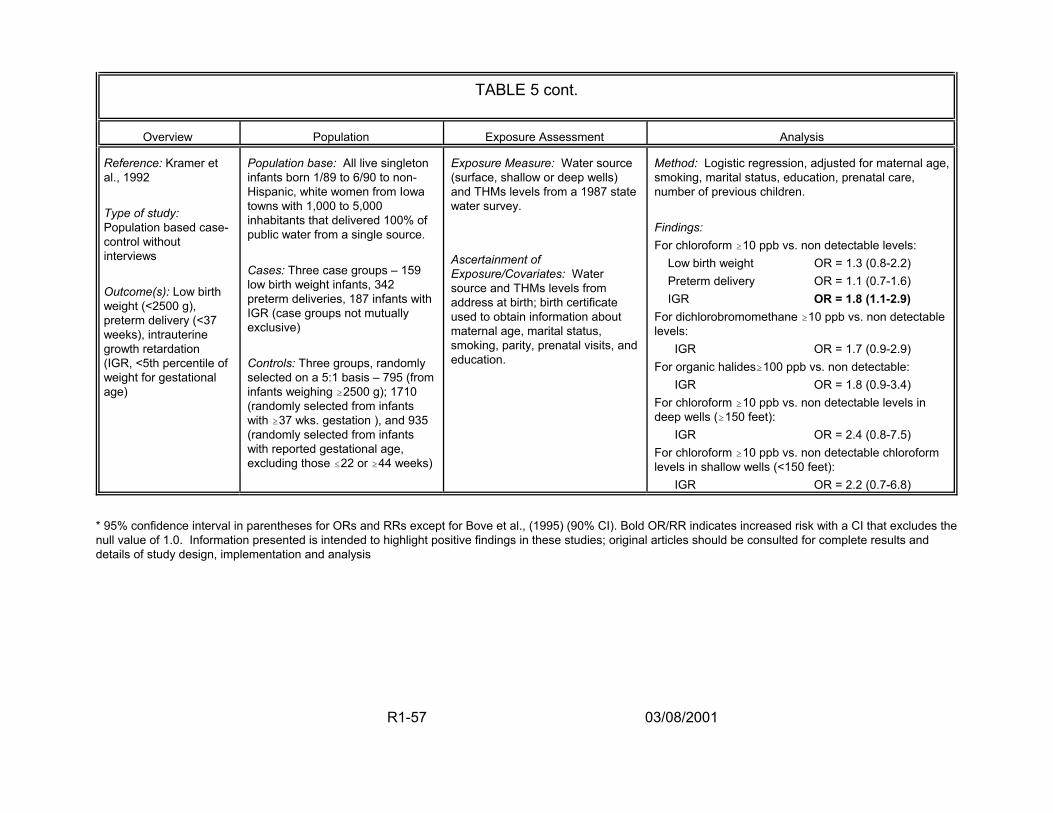
TABLE 5 cont.
Overview Population Exposure Assessment Analysis
Reference: Kramer et al., 1992
Type of study: Population based case-control without interviews
Outcome(s): Low birth weight (<2500 g), preterm delivery (<37 weeks), intrauterine growth retardation (IGR, <5th percentile of weight for gestational age)
Population base: All live singleton infants born 1/89 to 6/90 to non-Hispanic, white women from Iowa towns with 1,000 to 5,000 inhabitants that delivered 100% of public water from a single source.
Cases: Three case groups – 159 low birth weight infants, 342 preterm deliveries, 187 infants with IGR (case groups not mutually exclusive)
Controls: Three groups, randomly selected on a 5:1 basis – 795 (from infants weighing $2500 g); 1710 (randomly selected from infants with $37 wks. gestation ), and 935 (randomly selected from infants with reported gestational age, excluding those #22 or $44 weeks)
Exposure Measure: Water source (surface, shallow or deep wells) and THMs levels from a 1987 state water survey.
Ascertainment of Exposure/Covariates: Water source and THMs levels from address at birth; birth certificate used to obtain information about maternal age, marital status, smoking, parity, prenatal visits, and education.
Method: Logistic regression, adjusted for maternal age, smoking, marital status, education, prenatal care, number of previous children.
Findings: For chloroform $10 ppb vs. non detectable levels:
Low birth weight OR = 1.3 (0.8-2.2) Preterm delivery OR = 1.1 (0.7-1.6) IGR OR = 1.8 (1.1-2.9)
For dichlorobromomethane $10 ppb vs. non detectable levels:
IGR OR = 1.7 (0.9-2.9) For organic halides$100 ppb vs. non detectable:
IGR OR = 1.8 (0.9-3.4) For chloroform $10 ppb vs. non detectable levels in deep wells ($150 feet):
IGR OR = 2.4 (0.8-7.5) For chloroform $10 ppb vs. non detectable chloroform levels in shallow wells (<150 feet):
IGR OR = 2.2 (0.7-6.8)
* 95% confidence interval in parentheses for ORs and RRs except for Bove et al., (1995) (90% CI). Bold OR/RR indicates increased risk with a CI that excludes the null value of 1.0. Information presented is intended to highlight positive findings in these studies; original articles should be consulted for complete results and details of study design, implementation and analysis
R1-57 03/08/2001

increase in both number and quality before quantitative use of the results can be
considered.
2.4.2. Summary of Single Chemical Toxicology Studies. Taken as a body of
literature, single chemical toxicology studies on DBPs have produced effects in the
same target organ systems (but not always the same site) as those observed in the
positive epidemiology studies (i.e., for developmental and reproductive effects and
cancer). Toxicologic data are available for some of the more common DBPs, but not for
the hundreds of potential DBPs described in Section 2.3. As shown in Table 6,
information is available on the Agency’s Integrated Risk Information System (IRIS)
database (U.S. EPA, 2000b) for only a few DBPs; these are chloroform (CHCl3),
bromoform (CHBr3), bromodichloromethane (BDCM), chlorodibromomethane (CDBM),
dichloroacetic acid (DCA), trichloroacetic acid (TCA), formaldehyde and chloral hydrate
(CH), all of which have shown some evidence of carcinogenicity in the toxicologic
literature. Most of the data used to evaluate these DBPs are for oral exposures; little
information is available on the toxic effects of inhalation or dermal exposures. For these
DBPs and for an increasing number of additional DBPs, toxicologic studies are available
that show evidence of carcinogenicity, mutagenicity, reproductive and developmental
effects, hepatotoxicity, nephrotoxicity and other toxic effects in high-dose, single
chemical studies. (For more detailed information, see Section 2.3. of Report 2 and
Appendix I). This section highlights the toxicologic issues associated with individual
chemical studies of significant concern in the development of a DBP mixture risk
assessment.
R1-58 03/08/2001
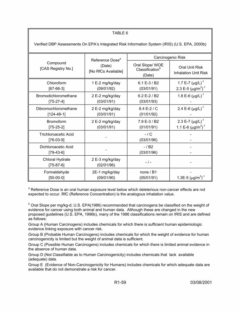
TABLE 6
Verified DBP Assessments On EPA’s Integrated Risk Information System (IRIS) (U.S. EPA, 2000b)
Carcinogenic Risk Compound
[CAS Registry No.]
Reference Dosea (Date)
[No RfCs Available] Oral Slope/ WOE
Classificationb (Date)
Oral Unit Risk Inhalation Unit Risk
Chloroform [67-66-3]
1 E-2 mg/kg/day (09/01/92)
6.1 E-3 / B2 (03/01/91)
1.7 E-7 (:g/L)-1 2.3 E-5 (:g/m3)-1
Bromodichloromethane [75-27-4]
2 E-2 mg/kg/day (03/01/91)
6.2 E-2 / B2 (03/01/93)
1.8 E-6 (:g/L)-1 -
Dibromochloromethane [124-48-1]
2 E-2 mg/kg/day (03/01/91)
8.4 E-2 / C (01/01/92)
2.4 E-6 (:g/L)-1 -
Bromoform [75-25-2]
2 E-2 mg/kg/day (03/01/91)
7.9 E-3 / B2 (01/01/91)
2.3 E-7 (:g/L)-1 1.1 E-6 (:g/m3)-1
Trichloroacetic Acid [76-03-9]
- - / C
(03/01/96) - -
Dichloroacetic Acid [79-43-6]
- - / B2
(03/01/96) - -
Chloral Hydrate [75-87-6]
2 E-3 mg/kg/day (02/01/96)
- / - -
Formaldehyde [50-00-0]
2E-1 mg/kg/day (09/01/90)
none / B1 (05/01/91)
- 1.3E-5 (:g/m3)-1
a Reference Dose is an oral human exposure level below which deleterious non-cancer effects are not expected to occur. RfC (Reference Concentration) is the analogous inhalation value. b Oral Slope per mg/kg-d; U.S. EPA(1986) recommended that carcinogens be classified on the weight of evidence for cancer using both animal and human data. Although these are changed in the new proposed guidelines (U.S. EPA, 1996b), many of the 1986 classifications remain on IRIS and are defined as follows: Group A (Human Carcinogens) includes chemicals for which there is sufficient human epidemiologic evidence linking exposure with cancer risk. Group B (Probable Human Carcinogens) includes chemicals for which the weight of evidence for human carcinogenicity is limited but the weight of animal data is sufficient. Group C (Possible Human Carcinogens) includes chemicals for which there is limited animal evidence in the absence of human data. Group D (Not Classifiable as to Human Carcinogenicity) includes chemicals that lack available (adequate) data. Group E (Evidence of Non-Carcinogenicity for Humans) includes chemicals for which adequate data are available that do not demonstrate a risk for cancer.
R1-59 03/08/2001

2.4.2.1. Carcinogenicity from Exposure to DBPs — The cancer process
involves several distinct events: initiation, promotion and progression. Chemical
carcinogens act through initiation and/or promotion; progression is related to the internal
biology of the tumor, governed largely by tumor type. Genotoxic chemical carcinogens
interact directly with the DNA and impart an initiating effect. This adverse change in
the DNA can be repaired or may remain long enough to be replicated and passed on to
daughter cells. These cells may then clonally expand to form tumors. Epigenetic
chemical carcinogens do not directly interact with the DNA of the organism, but alter
processes that govern cellular homeostasis. Disruption of cellular homeostasis allows
initiated cells to expand to become tumors. Tumor promoters (e.g., phthalates) are
carcinogens that may be encountered at doses predicted to be without adverse effect.
This type of carcinogen (epigenetic, tumor promoter) may demonstrate a distinct dose
level (threshold), below which the production of tumors is not evident.
As stated above, some evidence of carcinogenic response has been observed
for all of the DBPs in Table 6; the chemical-specific information presented here is found
on IRIS (U.S. EPA, 2000b). For the THMs, kidney tumors were seen in male rats
exposed to CHCl3. BDCM is structurally similar to other known animal carcinogens, is
mutagenic, and produced tumors at multiple sites in multiple species. CDBM is
mutagenic and produced liver tumors in female mice only at doses that also produced
liver damage. CHBr3 is genotoxic and induced neoplastic lesions in the large intestines
in rats. For the two haloacetic acids in Table 6, an increased incidence of
hepatocellular adenoma and carcinomas was found in male and female mice exposed
to DCA, and although TCA produced tumors in male and female mice, there is no
R1-60 03/08/2001
evidence of carcinogenicity in rats. Finally, squamous cell carcinomas were found in
male rats exposed to formaldehyde by inhalation. Although a cancer assessment is not
available on IRIS for CH, in a recent study, it was found to be carcinogenic
(hepatocellular neoplasia) in the male mouse, but not in the rat (George et al., 2000).
For several of these DBPs, however, questions regarding the strength of the
carcinogenic evidence remain. In particular, an expert panel cancer assessment (U.S.
EPA, 1998c) of CHCl3 that employed methodology from the 1996 proposed Cancer Risk
Assessment Guidelines (U.S. EPA, 1996b), found increasing evidence that the
carcinogenic mechanism of action for CHCl3 is not relevant at the low concentrations
found in drinking water. Similar issues are being raised for the haloacetic acids. In
addition, several of the THM cancer studies were performed using corn oil as the dosing
vehicle, confounding the carcinogenic results (see Section 2.4.2.3. below).
2.4.2.2. Developmental and Reproductive Effects from Exposure to
DBPs — Human epidemiologic studies identifying reproductive and developmental
toxicities have stimulated increased laboratory testing in this area. Qualitatively, DBPs
(especially, the haloacetic acids and haloacetonitriles) have been shown to adversely
affect reproduction and development in animals. Studies of reproductive and
developmental toxicity effects of DBPs, summarized elsewhere (and in EPA, 1999d),
demonstrated alterations in sperm morphology, motility and count; decreased levels of
fertility; spontaneous resorptions; decreased fetal body weight; and visceral,
cardiovascular and craniofacial malformations. Studies have shown alterations in
sperm parameters at the lowest doses tested. The haloacetic acids have also produced
male infertility in rats. Although effects on sperm morphology and/or motility indicate a
R1-61 03/08/2001

potential reproductive hazard, ascribing decreased fertility (a quantifiable measure of
adverse effect) to the test chemical may be somewhat conservative. Changes in sperm
motility, morphology or number do not necessarily translate into decreased fertility,
owing to the high degree of redundancy in sperm production. Nonetheless, these
observations are indicative of risk. Because of the epidemiologic link to cardiovascular
malformations in humans, animal studies were undertaken, through which confirmatory
data have been generated. Additional studies are aimed at investigating the potential
epidemiologic link between spontaneous abortion in humans and demonstrated
additional developmental toxicities with DBPs.
Seven of the 11 haloacetic acids (MCA, DCA, TCA, MCA) and haloacetonitriles
(DCAN, TCAN, BCAN) have been subjects of developmental toxicity studies by a single
group of investigators (e.g., Christ et al., 1995; Randall et al., 1991; Smith et al., 1988,
1989a,b, 1990, 1992). Three of the haloacetic acids (DCA, MBA, DBA) have been the
subjects of male reproductive studies by another group of investigators (e.g., Linder et
al.,1994) (see Sections 2.3. and 3.8. of Report 2 for references and additional details).
All of these studies were conducted in rats using gavage administration. The results for
developmental toxicity were positive. For reproductive toxicity, the dihalogenated
haloacetic acids gave positive results, but MBA gave negative results. An additional
chemical, the haloacetonitrile, DBAN, was tested in a short-term developmental and
reproductive toxicity screening study in rats by the NTP (1992), with negative results.
Evaluation of these data sets listed by dose-response modeling showed that visceral
malformations, particularly cardiovascular (interventricular septal defects, defects
between ascending aorta and right ventricle, and levocardia) and smaller fetal size
R1-62 03/08/2001
(body weight and crown-rump length) appeared to be the most sensitive endpoints in
common for these chemicals.
For the THMs, BDCM is of most concern for the developmental and reproductive
endpoints. An epidemiology study (Waller et al., 1998) associated exposures to BDCM
in the drinking water to spontaneous abortions. Klinefelter et al. (1995) reported that the
exposure of rats to BDCM in drinking water, significantly decreased sperm velocity. As
with the carcinogenic data, both the vehicle of administration and the possibility that the
mechanism of toxicity is not active at environmental exposure levels are of concern for
this data set.
2.4.2.3. Vehicle and Route Considerations — Toxicity data are often derived
from animal studies and generally include the administration of high doses of a
chemical. There is a crucial interplay between dose, dose rate, pharmacokinetics/
internal concentrations, mode/mechanism of action and saturable biologic processes.
The application of Haber’s Law (concentration times time) may not hold true for orally
administered compounds and for some compounds encountered via the inhalation
route. For instance, the administration of a single bolus delivered via gavage in a
vehicle that promotes rapid absorption of the chemical may produce absorption patterns
that would not be replicated in a human exposure to the same chemical via the same
route. Studies with CHCl3, BDCM, and the haloacetonitrile compounds have involved
the delivery of the chemicals via gavage in vehicles which may be problematic. For
example, CHCl3 administered as a single gavage bolus in corn oil produces peak
concentrations and toxicities greater or more detrimental than those observed from the
R1-63 03/08/2001
same dose (expressed as mg/kg/day) via drinking water spread over time through
multiple dosing (Simmons and Pegram, 1998).
While exposure to DBPs in drinking water is generally assumed to be through
ingestion of drinking water, the actual exposure pattern is more complex. Tap water is
used for cooking, washing household materials and showering/bathing. These uses
indicate that DBPs in drinking water are encountered via dermal and inhalation
pathways, as well as by ingestion. Although the DBPs encountered at low doses
through the consumption of drinking water are each virtually 100% bioavailable (they
are all absorbed with nearly 100% efficacy in the GI tract), the internal doses developed
as a function of inhalation or dermal exposure are not so uniform. In showering, both
the inhalation and dermal routes are relevant. Differential volatility and efficacy at which
DBPs are absorbed by the blood (governed by blood:air partitioning) largely determines
the internal doses attained from inhalation exposure. THMs have very low boiling
points, reasonably high vapor pressures, and low molecular weights. Thus, they readily
volatilize during showering or bathing. Jo et al. (1990) measured CHCl3 in breath
following showering while unclothed and clothed in a water-occlusive rubber suit.
Because CHCl3 in the exhaled breath of individuals wearing rubber suits was
approximately half that of individuals showering unclothed, these data may indicate that
(for CHCl3) the magnitude of dermal exposure is roughly equivalent to that from the
inhalation route. In contrast to CHCl3’s physical chemical properties (non-polar, well-
halogenated, highly lipophilic, highly volatile, low molecular weight) and high degree of
dermal penetration, the haloacetic acids, haloacetonitriles, and other higher molecular
weight DBPs have lower boiling points and vapor pressures and thus are volatilized with
R1-64 03/08/2001
much less efficiency. Thus, inhalation exposures favor the delivery of volatile DBPs
over non-volatile DBPs.
However, the dermal delivery of DBPs, is generally less well characterized. The
dermal absorption of CHCl3 in humans increases when CHCl3 in tap (bath) water was
encountered during bathing at higher temperatures than when bathing at lower
temperatures (Corley et al., 2000). Increased blood circulation to the skin promotes
higher absorbance of CHCl3. This physiological adaptation to heat likely increases the
absorbance of other DBPs, as well. Several factors distinguish the dermal penetrability
of chemicals, including DBPs. Higher degrees of lipophilicity promote dermal
absorbance. The lipophilicity of DBPs (measured as octanol:water partitioning, logP)
spanned a range of more than 100-fold. The degree to which lipophilicity dictates
dermal penetration indicates that the differential dermal absorption of DBPs produces
marked differences in their internal doses, even when encountered under similar
concentrations and conditions.
2.4.2.4. Pharmacokinetics and Target Organ Concentrations — While the
EPA regulates chemical exposures based on the dose expressed as milligrams
encountered per kilogram of body mass per day (mg/kg/day), the rate at which this dose
is encountered may significantly affect its toxicity. The administration of test chemicals
via the most likely route of human exposures is difficult when actual exposures may be
through drinking water encountered over the course of a day. Although investigators
can maintain the same route (oral) by dissolving the chemical in a dosing vehicle (water,
corn or olive oil, tricaprylin, etc.) and administering it orally, the rate at which these
chemicals enter the body and the resulting internal concentrations of the chemical in
R1-65 03/08/2001
target organs for toxicity differ from those produced by the same daily dose (mg/kg/day)
delivered in multiple, lower doses (e.g., hepatic concentrations of CHCl3 resulting from
temporally-dispersed drinking water exposure are lower than those resulting from a
bolus corn oil gavage exposure). This sometimes marked difference in internal
concentrations may affect toxic response through several mechanisms; two examples
hinge on metabolism and cellular damage.
Attaining higher internal concentrations (resulting from higher doses) of a toxicant
can recruit additional (or secondary) enzymes to the disposition of chemicals. This can
result in the production of qualitatively different (and differentially toxic) metabolites at
higher doses than at lower doses. This may become evident when doses, potentially
spread over the course of a day, are concentrated into a single dose and administered
in a vehicle promoting rapid absorption and delivery to tissues. On the other hand,
some chemicals may be metabolized, regardless of dose, to produce toxic metabolites.
However, lower concentrations of the toxic metabolites may produce cellular responses
that can be corrected by the normal functioning of the cell. Cellular damage and
necrosis can be repaired (or replaced) to some degree, but when the extent of injury
increases the rate of cellular replication to the point that efficient DNA repair (a normal
function) cannot take place, then the potential for mis-formation of DNA and genetic
damage exists. This mis-formation of DNA can lead to the development of cancer. This
phenomenon may complicate the extrapolation of high dose toxicity to lower doses, and
makes the identification of the mode of action (MOA) all the more critical. Certainty
about potential dose-dependency of the MOA reduces uncertainty in the extrapolation to
lower doses.
R1-66 03/08/2001
For several chemicals whose toxicity is mediated through a common MOA, and
that may be encountered in combination, an estimate of their combined toxicity may be
accomplished by combining their doses. In addition to information on MOA,
pharmacokinetic information about the chemicals allows for a more thorough evaluation
of the toxic interaction of mixtures, regardless of their MOA. When these chemicals are
active in their parent form, their metabolism reduces their toxic impact. However, one of
the chemicals may reduce the body’s ability to metabolize the others, resulting in
prolonged residence time in the body and greater opportunity for interaction with
biological (target) tissues. The elucidation of general and specific pharmacokinetic
parameters thus enhances the ability to ascertain or estimate the effect of multiple
chemical exposures.
2.4.2.5. Mode of Action — Determination of MOA and any dose-dependency of
the MOA is helpful when evaluating dose-response. BDCM’s carcinogenic response
may involve metabolism through the glutathione S-transferase pathway, but this may
not be relevant at low doses or low internal concentrations. BDCM produces genetic
damage in bacteria into which rat glutathione S-transferase theta class enzyme has
been transfected, but not in the same bacterial strain lacking this enzyme (DeMarini et
al., 1997). In mammals, lower doses of BDCM are metabolized by the mixed function
oxidase system, but higher doses of BDCM may saturate this mechanism and recruit
the glutathione S-transferase metabolic system. Thus, the delivery of the test chemical
via methods that may not mimic the human exposure scenario may produce results that
must be carefully extrapolated to humanly-relevant doses and delivery schedules. This
differential effect with respect to dose (target organ concentration) has been recognized
R1-67 03/08/2001
in the Agency’s treatment of CHCl3 risk; is being investigated with respect to BDCM risk;
and complicates the interpretation of developmental toxicity results obtained with
haloacetonitrile compounds delivered via gavage in tricaprylin. The results obtained
from research animals treated via gavage with boli of high doses of toxicants may
provide overly conservative estimates of risk when extrapolated to humans in the
absence of adequate pharmacokinetic, metabolism and MOA considerations.
2.4.2.6. Bromate — When source waters are high in bromide and ozone is the
primary chemical disinfectant, brominated compounds are produced in greater
quantities than chlorinated DBPs; bromate, in particular, is produced. Drinking water
studies of rats exposed to bromate have shown the production of kidney tumors (males
and females) and peritoneal mesotheliomas (males only) (Kurokawa et al., 1983).
Although these results indicate that bromate is a complete carcinogen, additional
experiments in this study demonstrated its tumor promoting activity in the kidney and
that the lowest dose producing kidney tumors was 6.5 mg/kg/day (doses employed
were 0.7, 1.3, 2.5, 5.6, 12.3 and 33.4 mg/kg/day). Interestingly, no increase in liver
tumors followed initiating treatment (with EHEN). Kurata et al. (1992) treated rats with
acute doses of bromate followed by promoting doses of barbital sodium to examine
tumor initiating activity, but could demonstrate none. The lack of tumor initiating activity
may support the theory that longer durations are necessary to initiate tumors or that
bromate produces renal tumors through promotional activity.
An evaluation of the impact of bromate (delivered as either KBrO3 or NaBrO3)
indicates that these chemicals, but not KBr, induce alpha-2-micro-globulin accumulation
in the kidneys of male, but not female, rats (Umemura et al., 1993). These data,
R1-68 03/08/2001

coupled with the lack of renal carcinogenicity in mice and hamsters (Kurokawa et al.,
1986; Takamura et al., 1985), raise the question of the relevancy of bromate-induced
renal tumors to the evaluation of cancer risk in humans. The involvement of alpha-2-
micro-globulin as an exclusive mechanism of tumorigenicity in rat kidneys is confounded
by the finding of renal tumors in female rats (Kurokawa et al., 1983). Alternately, the
production of oxidative stress in renal tissue may stimulate cell replication, resulting in
tumor promotion (Umemura et al., 1995). Although the finding of renal tumors in
female rats may reduce the perceived importance of alpha-2-micro-globulin as an event
modifying renal carcinogenicity, its association with male rat kidney tumors may indicate
that the mechanism may increase the incidence of tumors in male rats beyond the
incidence in female rats. This may raise questions about the validity of carcinogenic
risk estimates for bromate, as they are mainly based on the incidence and dose-
response relationship demonstrated for male rat kidney tumors.
Consistent with the finding of renal toxicity in rodents, humans acutely exposed
to bromate (potassium and/or sodium bromate) in permanent hair wave neutralizing
solutions have demonstrated severe renal damage as well as permanent hearing loss.
There are no available published reports on the potential of bromate to produce
developmental toxicity. Recently, published data (DeAngelo et al., 1998) have
confirmed the multisite carcinogenicity of bromate in rats. A slight dose-response was
noted for kidney tumors in mice. The U.S. EPA (2000b) has considered this evidence
supportive of earlier MCL (0.01 mg/L) and MCLG (zero) values.
Bromate also produces oxidative injury in tissues, as evidenced by the formation
of characteristic 8 hydroxy-deoxyguanine adducts. Oxidative stress may be a tumor
R1-69 03/08/2001
promotional event. DeAngelo and co-workers (Crosby et al., 2000; DeAngelo et al.,
1998; and Wolff et al.,1998) have examined the effect of potassium bromate on tumors
other than kidney in rats and mice. They have demonstrated that bromate induces a
high number of tumors in the tunica vaginalis of the testicle of rats, and that these
tumors can spread through the mesentary to other parts of the viscera. Tumor
prevalence at this site was 25% in a 2-year bioassay, while only 1% of rats
demonstrated renal carcinogenicity. These results identify a site much more sensitive
to carcinogenesis than the kidney and offer additional carcinogenesis dose-response
data for risk assessment considerations. These authors pointed out the unique
anatomy and physiology of this tumor site, and recommend specific attention to those
factors that may uniquely influence toxicity/carcinogenicity at this site.
2.4.3. Summary of Mixtures Toxicology In Vivo and In Vitro Studies. A number of
toxicology studies are available on mixtures of DBPs, ranging across a variety of
effects, including mutagenicity, carcinogenicity, hepatotoxicity, nephrotoxicity,
developmental toxicity, neurological effects and changes in pharmcokinetics (Table 7).
Historically, the majority of research with DBP mixtures has focused on toxicologic
assessment of concentrated drinking water samples, with an emphasis on detection of
mutagenicity. In the 1990s, there has been an increased interest in research on simple
DBP mixtures, with a general focus on interactions either among the trihalomethanes
(THMs) or among the haloacetic acids (HAAs). This initial focus on the within-class
interactions among the THMs and the HAAs is understandable because the vast
majority of single-chemical toxicology research on DBPs has focused on these two
important chemical classes, resulting in the identification of carcinogenic,
R1-70 03/08/2001
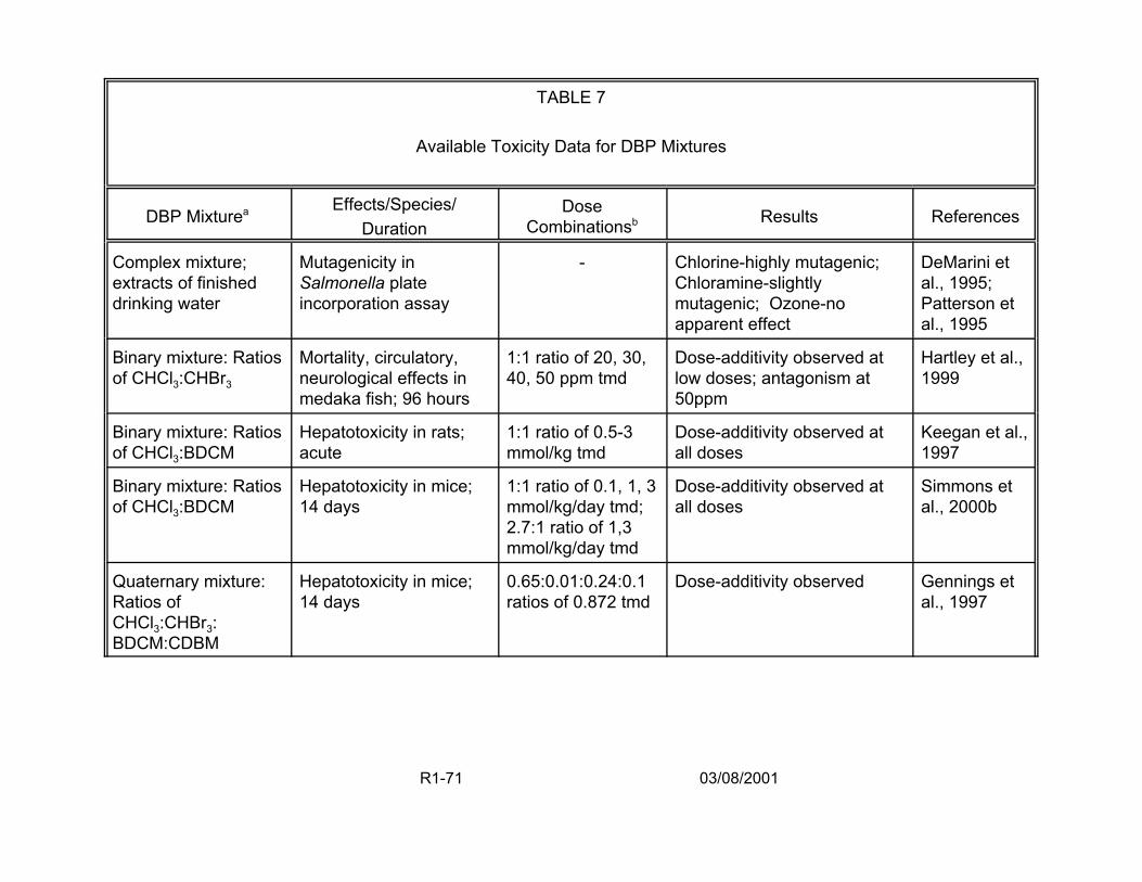
TABLE 7
Available Toxicity Data for DBP Mixtures
DBP Mixturea Effects/Species/ Duration
Dose Combinationsb Results References
Complex mixture; extracts of finished drinking water
Mutagenicity in Salmonella plate incorporation assay
- Chlorine-highly mutagenic; Chloramine-slightly mutagenic; Ozone-no apparent effect
DeMarini et al., 1995; Patterson et al., 1995
Binary mixture: Ratios of CHCl3:CHBr3
Mortality, circulatory, neurological effects in medaka fish; 96 hours
1:1 ratio of 20, 30, 40, 50 ppm tmd
Dose-additivity observed at low doses; antagonism at 50ppm
Hartley et al., 1999
Binary mixture: Ratios of CHCl3:BDCM
Hepatotoxicity in rats; acute
1:1 ratio of 0.5-3 mmol/kg tmd
Dose-additivity observed at all doses
Keegan et al., 1997
Binary mixture: Ratios of CHCl3:BDCM
Hepatotoxicity in mice; 14 days
1:1 ratio of 0.1, 1, 3 mmol/kg/day tmd; 2.7:1 ratio of 1,3 mmol/kg/day tmd
Dose-additivity observed at all doses
Simmons et al., 2000b
Quaternary mixture: Ratios of CHCl3:CHBr3: BDCM:CDBM
Hepatotoxicity in mice; 14 days
0.65:0.01:0.24:0.1 ratios of 0.872 tmd
Dose-additivity observed Gennings et al., 1997
R1-71 03/08/2001
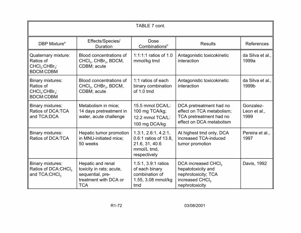
TABLE 7 cont.
DBP Mixturea Effects/Species/ Duration
Dose Combinationsb Results References
Quaternary mixture: Ratios of CHCl3:CHBr3: BDCM:CDBM
Blood concentrations of CHCl3, CHBr3, BDCM, CDBM; acute
1:1:1:1 ratios of 1.0 mmol/kg tmd
Antagonistic toxicokinetic interaction
da Silva et al., 1999a
Binary mixtures: Ratios of CHCl3:CHBr3: BDCM:CDBM
Blood concentrations of CHCl3, CHBr3, BDCM, CDBM; acute
1:1 ratios of each binary combination of 1.0 tmd
Antagonistic toxicokinetic interaction
da Silva et al., 1999b
Binary mixtures: Ratios of DCA:TCA and TCA:DCA
Metabolism in mice; 14 days pretreatment in water, acute challenge
15.5 mmol DCA/L: 100 mg TCA/kg; 12.2 mmol TCA/L: 100 mg DCA/kg
DCA pretreatment had no effect on TCA metabolism; TCA pretreatment had no effect on DCA metabolism
Gonzalez-Leon et al., 1999
Binary mixtures: Ratios of DCA:TCA
Hepatic tumor promotion in MNU-initiated mice; 50 weeks
1.3:1, 2.6:1, 4.2:1, 0.6:1 ratios of 13.8, 21.6, 31, 40.6 mmol/L tmd, respectively
At highest tmd only, DCA increased TCA-induced tumor promotion
Pereira et al., 1997
Binary mixtures: Ratios of DCA:CHCl3 and TCA:CHCl3
Hepatic and renal toxicity in rats; acute, sequential, pre-treatment with DCA or TCA
1.5:1, 3.9:1 ratios of each binary combination of 1.55, 3.08 mmol/kg tmd
DCA increased CHCl3 hepatotoxicity and nephrotoxicity; TCA increased CHCl3 nephrotoxicity
Davis, 1992
R1-72 03/08/2001
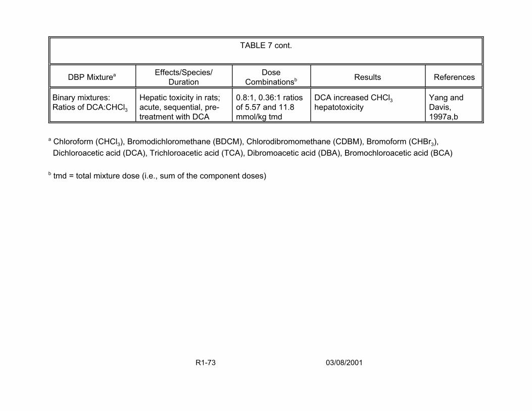
TABLE 7 cont.
DBP Mixturea Effects/Species/ Duration
Dose Combinationsb Results References
Binary mixtures: Ratios of DCA:CHCl3
Hepatic toxicity in rats; acute, sequential, pre-treatment with DCA
0.8:1, 0.36:1 ratios of 5.57 and 11.8 mmol/kg tmd
DCA increased CHCl3 hepatotoxicity
Yang and Davis, 1997a,b
a Chloroform (CHCl3), Bromodichloromethane (BDCM), Chlorodibromomethane (CDBM), Bromoform (CHBr3), Dichloroacetic acid (DCA), Trichloroacetic acid (TCA), Dibromoacetic acid (DBA), Bromochloroacetic acid (BCA)
b tmd = total mixture dose (i.e., sum of the component doses)
R1-73 03/08/2001
developmental, hepatotoxic and nephrotoxic effects of concern. In addition, the THMs
and HAAs are among the most commonly occurring DBPs and are present at relatively
high concentrations compared to other DBPs. One notable exception to the within-class
investigations has been examination of the effect of dichloroacetic acid (DCA, a
HAA) on chloroform (CHCl3, a THM ) toxicity.
The generation of DBP mixtures data is essential to refine human health risk
assessment methods under development and efficient experimental designs and
statistical approaches for mixtures (Simmons et al., 2000a; Teuschler et al., 2000).
Because several available risk assessment methods are based on additivity
assumptions, their use to estimate DBP mixtures risk should be grounded by toxicity
data supporting these assumptions. Although the number of studies on defined DBP
mixtures is still small, several conclusions may be drawn from this body of literature.
First, the nature of the observed interaction (additive, nonadditive) may depend on
whether the multiple chemical exposure is concurrent or temporally separated. Second,
the mixing ratio of the components comprising the mixture may affect the toxic outcome
and account for apparent inconsistencies across studies. Third, interactive effects
appear to be dose-dependent (e.g., synergism and antagonism are expected interaction
effects at high dose levels, while dose additivity is more commonly observed in lower
portions of the mixture dose-response curve). This dose-dependence may account for
inconsistencies across studies that appear to have conflicting outcomes, but are
actually working in different sections of the dose-response curve. In general, these
conclusions are consistent with the current state of knowledge in mixtures research.
R1-74 03/08/2001

2.4.3.1. Complex Mixtures of DBPs — DeMarini et al. (1995) and Patterson et
al. (1995) examined the mutagenic potency of extracts prepared from water that had
undergone one of several different disinfection treatments. The DBPs present in the
drinking water were concentrated by extraction techniques that resulted in concentration
of the semi-volatile and nonvolatile organics and the loss of the volatile organics.
Mutagenicity was assessed in the Salmonella plate incorporation assay (Patterson et
al. employed strains TA100, TA98, TA97 and TA102, with and without metabolic
activation, and DeMarini et al. used strains TA98 and TA100 without metabolic
activation).
According to their findings, raw water (i.e., water that has not undergone
chemical disinfection) has a very low level of mutagenic activity. Compared to raw
water, chlorination greatly increases the mutagenicity of water. Ozonation alone has
very little apparent effect on the mutagenic activity of water. Chloramination alone
increases the mutagenicity of water, but to a lesser extent than chlorination. Prior
treatment with ozone decreases the mutagenicity associated with either chloramination
or chlorination. Generally, the addition of metabolic activation decreases mutagenic
activity. The mutation spectra produced by the various drinking water extracts resemble
those produced by MX (3-chloro-4(dichloromethyl)-5-hydroxy-2(5H)-furanone, a highly
mutagenic DBP).
2.4.3.2. Defined Mixtures of Trihalomethanes — To date, the binary
combination of CHCl3 and bromoform (CHBr3) has been evaluated in a Japanese
medaka (Oryzias latipes) embryo lethality/developmental toxicity assay and the binary
combination of CHCl3 and bromodichloromethane (BDCM) has been examined for
R1-75 03/08/2001
hepatotoxicity in both mice and rats. In the fish assay, medaka were exposed
concurrently to CHCl3 and CHBr3 for 96 hours (Hartley et al., 1999). The measured
effect was based on the combined incidence of death and severe
neurological/circulatory effects expected to result in death. The data were analyzed
using a response surface model (Gennings et al., 1997), built under the assumption of
dose-addition, and then used to test for departures from dose additivity. Of the four
concentrations tested at a 1:1 mixing ratio of CHCl3:CHBr3, deviation from dose
additivity was detected only at the highest tested concentrations of 25 ppm CHCl3: 25
ppm CHBr3, where antagonism was observed. At all lower concentrations (10:10,
15:15, 20:20), the toxicity of the mixtures did not depart from that predicted by dose
additivity.
The binary interaction of CHCl3 and BDCM was evaluated in mice (female, CD-1)
and rats (male, F-344) following concurrent oral exposure in an aqueous vehicle
(Keegan et al., 1997; Simmons et al., 2000b). Hepatotoxicity was assessed by serum
indicators of hepatic damage in rats 24 hours after acute exposure and in mice after 14
days of daily dosing. Rats were exposed to total mixture dosages ranging from 0.5 to
3.0 mmol/kg at a 1:1 mixing ratio. In the mouse experiment, three mixture groups were
exposed to total mixture dosages of either 0.1, 1.0 or 3.0 mmol/kg/day at a mixing ratio
of 1:1 CHCl3:BDCM; another two mixture groups were exposed to total mixture dosages
of either 1.0 or 3.0 mmol/kg/day at a mixing ratio of 2.7:1 CHCl3:BDCM. The 2.7:1
mixing ratio of CHCl3:BDCM was selected based on the average seasonal proportions
of these two chemicals at 35 U.S. water treatment facilities (Krasner et al., 1989). In
R1-76 03/08/2001
both species, there was little or no apparent deviation from dose additivity at the tested
mixing ratios and chemical concentrations.
The hepatotoxicity of a mixture of the four THMs (CHCl3, CHBr3, BDCM, and
chlorodibromomethane [CDBM]) has been evaluated (Gennings et al., 1997, 1999) in
mice under an experimental protocol similar to that described above for the binary
combination of CHCl3 and BDCM. The four THMs were administered in an aqueous
vehicle to female CD-1 mice by concurrent daily oral exposure for 14 days. The mixing
ratio of the four THMs was selected based on their average seasonal proportions at 35
U.S. water treatment facilities (Krasner et al., 1989). The proportions, on a mmol basis,
were 0.65 CHCl3: 0.01 CHBr3: 0.24 BDCM: 0.10 CDBM. The total mixture dosage was
0.872 mmol/kg/day. The threshold additivity model was used to predict the serum level
of sorbitol dehydrogenase (SDH), a serum indicator of hepatotoxicity, expected under
an assumption of dose additivity. The predicted mean SDH value for the mixture was
40.5 IU/l with 95% prediction limits of 31.9 and 49.1. The experimental mean SDH
response was 43.9 IU/l. The close correspondence between the predicted and the
observed mixture response indicated that hepatotoxicity, as measured by this serum
indicator, did not deviate from the level predicted under dose additivity.
In contrast to the dose additivity reported for the hepatotoxicity of the four THMs
(Gennings et al., 1997), other investigators (da Silva et al., 1999a) have reported an
apparent antagonistic toxicokinetic interaction among the four THMs. Male Sprague-
Dawley rats were exposed acutely by oral administration to 0.25 mmol/kg of each THM
alone or to a four-THM mixture containing 0.25 mmol/kg of each chemical for a total
mixture dosage of 1.0 mmol/kg. For each THM, administration in the mixture resulted in
R1-77 03/08/2001
increased blood concentrations when compared to single chemical administration,
indicating decreased metabolism. Work in progress (da Silva et al., 1999b) has
compared, for all six possible binary combinations of the four THMs, blood THM
concentration following oral exposure to 0.5 mmol/kg of each THM alone with the blood
THM concentration resulting from exposure to binary combinations at a total mixture
dosage of 1.0 mmol/kg (i.e., containing 0.5 mmol/kg of each THM). Similar to what was
seen with the four-THM mixture, exposure to the THMs in binary combination resulted in
an increase in blood concentration when compared to single chemical administration.
Several reasonable hypotheses can be constructed to explain the apparent
conflict between the dose additivity among the THMs for hepatotoxicity based on serum
indicators reported by Simmons et al. (2000b) and the metabolic antagonism among the
THMs reported by da Silva et al. (1999a) One explanation may lie in the definition of
additivity applied in these studies. The conclusions drawn by Simmons et al. are based
on the concept of dose addition. Although the underlying model of additivity used by da
Silva et al. is not stated, the results of their work appear to be based on the concepts of
response or effect addition. These models of chemical interaction are based on
different mathematical constructs and toxicological assumptions about mechanism of
action (U.S. EPA, 1986, 1999c). Thus, they do not necessarily result in the same
conclusion regarding additivity or nonadditivity (Gessner, 1988).
Another possible hypothesis lies with the endpoints chosen for examination.
Serum indicators such as SDH are generally considered sensitive markers of
hepatotoxicity; it is possible that other measures of hepatotoxicity would respond
differently. The two research groups used different species and strains/stocks of
R1-78 03/08/2001
animals and the differing results may reflect either species or strain differences in
chemical response. Rarely has the same mixture or multiple chemical exposure been
tested in more than one species or strain. Finally, differences in chemical interactions
between these studies could be the result of differences in the mixing ratios employed.
Simmons et al. used environmentally-based ratios that included very small proportions
of CHBr3 (1% of the mixture, for an actual dosage of 0.012 mmol/kg/day), a relatively
toxic THM. In contrast, da Silva et al. used a 1:1 mixing ratio, resulting in much larger
dosages of CHBr3, namely, 0.25 and 0.5 mmol/kg.
2.4.3.3. Defined Mixtures of Haloacetic Acids — Gonzalez-Leon et al. (1999)
examined the effect of pretreatment with DCA on the pharmacokinetics of trichloroacetic
acid (TCA) in male B6C3F1 mice. Similarly, they examined the effect of pretreatment
with TCA on the kinetics of DCA. Mice were exposed for 14 days to drinking water
containing either 2 g DCA/L (~15.5 mmol DCA/L) or water containing 2 g TCA/L (~12.2
mmol TCA/L). On the 15th day, the DCA pretreated mice were challenged with 100 mg
TCA/kg, and the TCA-pretreated mice were challenged with 100 mg DCA/kg. The
authors found pretreatment with DCA had no apparent effect on TCA metabolism, and
pretreatment with TCA had little or no apparent effect on DCA metabolism.
Pereira et al. (1997) assessed hepatic tumor promotion in methyl-nitrosourea
(MNU)-initiated female B6C3F1 mice that had been exposed chronically to mixtures of
TCA and DCA via their drinking water. The mice were initiated at 15 days of age with
MNU; they received DCA alone (7.8, 15.6 or 25 mmol/L), TCA alone (6.0 or 25 mmol/L)
or mixtures of DCA and TCA (7.8 mmol DCA/L + 6.0 mmol TCA/L, 15.6 mmol DCA/L +
6.0 mmol TCA/L, 25 mmol DCA/L + 6.0 mmol TCA/L, 15.6 mmol DCA/L + 25 mmol
R1-79 03/08/2001
TCA/L) in the drinking water from 6 to 50 weeks of age. With response expressed on a
per mouse basis (altered hepatic foci/mouse and total hepatic proliferative
lesions/mouse), the authors reported that 6.0 mmol TCA/l had little effect on DCA-
induced tumor promotion in mice that received either 7.8, 15.6 or 25 mmol DCA/L. DCA
at 15.6 mmol/L appeared to increase TCA-induced tumor promotion in mice that
received 25 mmol TCA/L but not in mice that received 6.0 mmol TCA/L. Experiments
are in progress to test the effect of binary combinations of CHCl3 and DCA or CHCl3 and
TCA on hepatic tumor promotion (Pereira and Kramer, 1999).
Comparing the work of Pereira et al. with that of Gonzalez-Leon et al., it can be
noted that these two research groups are investigating different regions of the TCA
dose-response curve. The dose level of TCA appears to affect whether DCA enhances
TCA-induced tumors. DCA had no detectable enhancing effect in combination with 6.0
mmol TCA/L but has an apparent enhancing effect at 25 mmol TCA/L. The dose level
of TCA, 25 mmol/L, at which an apparently greater than additive effect on tumor
promotion occurred is 2-fold higher than the dose of TCA shown to have little or no
effect on DCA metabolism.
2.4.3.4. Defined Mixtures of Trihalomethanes and Haloacetic Acids — In the
only example of cross-class mixtures of DBPs found, Davis (1992) examined the
effects of pretreatment with either DCA or TCA on CHCl3 hepatic and renal toxicity in
male and female Sprague-Dawley rats. Pretreatment with DCA (administered by
gavage 27, 10 and 3 hours prior to CHCl3) at 0.92 mmol DCA/kg (but not 2.45 mmol
DCA/kg) increased CHCl3 (~0.63 mmol CHCl3/kg by i.p. injection) hepatic toxicity 24
hours after CHCl3 administration. Both 0.92 and 2.45 mmol DCA/kg increased the
R1-80 03/08/2001
nephrotoxicity of this dosage of CHCl3. A similar pretreatment regimen with TCA at 2.45
mmol TCA/kg (but not at 0.92 mmol TCA/kg) enhanced the renal, but not the hepatic,
toxicity of CHCl3 (~0.63 mmol CHCl3/kg), 24 hours after CHCl3 administration. The
enhancement of CHCl3 toxicity by the HAAs was gender specific, with increased toxicity
seen in female, but not male, rats. Further experimentation with the same rat stock
(female and male Sprague-Dawley) with DCA revealed that pretreatment with 2.45
mmol DCA/kg (27, 10 and 3 hours prior to CHCl3) resulted in increased hepatic toxicity
at both 3.12 and 9.35 mmol CHCl3/kg in female rats and at 3.12 mmol CHCl3/kg in male
rats (Yang and Davis, 1997a). In addition to the differences in CHCl3 dosage between
these two studies, the nutritional status of the rats differed; Davis (1992) rats received
feed ad libitum whereas the Yang and Davis (1997a) rats were fasted for 20 hours prior
to CHCl3 administration.
Based on the results of a series of experiments (Yang and Davis, 1997a,b; Yang
et al., 1996), the mechanism by which DCA potentiates CHCl3 hepatotoxicity appears to
be linked to hepatic CYP2E1 induction by DCA. Treatment with DCA under the same
dosage regimen used in the interaction studies (2.45 mmol DCA/kg, 27, 10 and 3 hours
prior to termination) resulted in increased hepatic CYP2E1 activity as measured by both
aniline hydroxylation and p-nitrophenol hydroxylation and in increased amounts of
CYP2E1 protein as measured by immunoblot analysis (Yang et al., 1996). As the
concentration of 3-hydroxybutyrate was also increased, the induction of hepatic
CYP2E1 may be an indirect effect of DCA (Yang et al., 1996). Research to elucidate
the mechanism(s) underlying nonadditive interactions is important, because a
mechanistic understanding provides a rational basis for extrapolation of toxicologic
R1-81 03/08/2001

information across dose, route, length of exposure, and to other species (Simmons,
1994, 1995b). This dose-dependence may account for inconsistencies across studies
that appear to have conflicting outcomes, but are actually working in different sections
of the dose-response curve. In general, these conclusions are consistent with the
current state of knowledge with regard to mixtures research. For risk assessment
purposes, the behavior of multiple chemicals at low dose levels is critical to support the
methodology used to assess health risks.
2.5. THE UNIDENTIFIED FRACTION OF DBPS
As illustrated in Figure 4, generally more than half the DBPs in drinking water
consist of unidentified material, yet measures of the concentrations and potential toxicity
of such material are critical to performing a risk assessment. Measures generally
available include: Total Organic Carbon (TOC); DBPs routinely monitored either
individually or as summary concentrations (e.g., total THMs, HAAs); and Total Organic
Halides (TOX). Although it is not standard practice, methods are available to proportion
the TOX into total organic chlorine (TOCl) and total organic bromine (TOBr). These
distinctions are important because when source waters high in bromide are treated with
ozone or chlorine, higher levels of the brominated compounds are produced. Concern
over the toxicity of brominated compounds has increased as newer epidemiology and
toxicology data indicate these compounds may be more toxic than their chlorinated
analogues. The formation of bromate, a highly toxic DBP, is of particular concern
because it can be formed in relatively large amounts as a by-product of ozonation
processes applied to high bromide source water.
R1-82 03/08/2001
DBPs can be divided into three groups that reflect their analytic chemistry (Figure
5). A small number of halogenated DBPs (Group A), which account for up to 50% of the
total organic halides in treated drinking water, can be quantitated by routine gas
chromatography (GC). Examples of Group A DBPs are reported by Miltner et al. (1990)
and Weinberg (1999). The set of halogenated DBPs that cannot be quantitated by
routine GC comprises Group B. Several hundred Group B DBPs have been identified
qualitatively through GC and mass spectrometry (MS), but most of them have not been
quantitatively measured. Examples of Group B DBPs are reported by Richardson
(1998). Other members of Group B are suspected to be present in drinking water but
have not yet been identified. Finally, a third group consisting of non-halogenated
organic compounds (Group C) also exists. Some members of Group C have been
identified, but many others are suspected to be present in drinking water but remain
identified to date. The measured TOX concentration can be used to identify the quantity
of material that comprises Group B. The organic halogen concentration of each member
of Group A can be quantified and summed, yielding the fraction of the TOX
concentration that may be accounted for by Group A. The organic halide concentration
associated with Group B is the difference between the TOX and the organic halide
concentration associated with Group A. In general, some Group C DBPs are measured
individually (e.g., formaldehyde), and TOC is also measured routinely.
Assessing the risks posed by exposures to Group B compounds is complicated
because 1) all members of Group B have probably not been identified; 2) the quantity of
each component is not known; and 3) the toxicity of most of the compounds that have
R1-83 03/08/2001
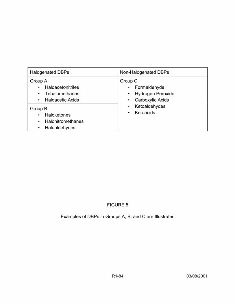
Halogenated DBPs Non-Halogenated DBPs
Group A • Haloacetonitriles • Trihalomethanes • Haloacetic Acids
Group C • Formaldehyde • Hydrogen Peroxide • Carboxylic Acids • Ketoaldehydes • Ketoacids
Group B • Haloketones • Halonitromethanes • Haloaldehydes
FIGURE 5
Examples of DBPs in Groups A, B, and C are Illustrated
R1-84 03/08/2001
been found has not been tested in bioassays. If it is assumed that the toxicity of those
Group B compounds identified through GC and MS (from the same drinking water
sample as the Group A compounds) is representative of the toxicity of the entire Group
B, then the toxic potential of individual compounds in this set can be estimated by
Quantitative Structure Toxicity Relationship (QSTR) models (e.g., Moudgal et al., 2000).
Such models predict toxicologic bioassay results for untested substances based on the
degree of similarity between the molecular attributes of the untested compound and
previously tested compounds.
2.6. RISK ASSESSMENT USING A RESPONSE ADDITION APPROACH
The initial assessment illustrates how DBP mixture risk may be quantified using a
two-stage Monte Carlo analysis of DBP occurrence data, DBP toxicity estimates, and
human drinking water consumption rate data (U.S. EPA, 1998a, 1999a). (The details of
this risk characterization, including exposure estimates, toxicity values and risk
estimates, are presented in full in Appendix I; presentations of this analysis from the
workshop are summarized in Section 2. of Report 2.) The drinking water source was a
pilot-scale drinking water treatment plant (Miltner et al., 1990), designed to simulate
several drinking water treatment system configurations. Two of these for which risk
estimates were developed included a conventional chlorination treatment system and a
pre-ozonation system followed by a conventional chlorination treatment system.
This illustration was developed as a limited demonstration to evaluate: 1)
whether sufficient data exist on exposure and toxicity to estimate DBP mixture risks; 2)
if response addition is a reasonable risk assessment method for this effort; and 3) how
to address and present the uncertainty and variability in the available data. Through the
R1-85 03/08/2001

development of a reasonable set of assumptions regarding two hypothetical drinking
water treatment interventions and the potential toxicity of the DBP mixtures, the
illustration shows that facility-specific data can be input to the response addition model
to develop DBP mixtures risk estimates for a drinking water treatment system. This
illustration highlights critical areas where pertinent research could potentially change the
outcomes of the analysis. The constraints of the illustration include the following:
• Comparison of only two alternative drinking water treatment technologies and no comparison of gradations of application (e.g., changes in the levels of chlorination or ozone)
• Limitations of available input data for DBP concentrations and toxicity values and tap water consumption rates to develop distributions for conducting an uncertainty analysis
• Constraints concerning the current scientific measurement and the temporal distribution of concentrations of DBPs in treated drinking water from a single treatment system. Additionally, no attempt has been made to characterize the impact of the water distribution system on estimated DBP concentrations
• Limitations in the understanding of the relationship between health effects and DBP exposures through drinking waters inherent in the risk assessments of these agents both collectively and individually
• Evaluation of systems functioning normally without taking into account scenarios that may result from perturbation(s) or critical failures of the drinking water treatment plant.
In this approach, epidemiologic and toxicologic data were used in the hazard
identification to identify the nature of the hazard posed by DBPs. In this case, cancer,
reproductive and developmental effects were identified to be of concern from DBP
exposures using both the epidemiologic and toxicologic data as corroborating evidence.
Only the DBP toxicology data were used in the dose-response assessment; however,
R1-86 03/08/2001
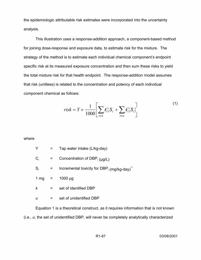
i ui k
the epidemiologic attributable risk estimates were incorporated into the uncertainty
analysis.
This illustration uses a response-addition approach, a component-based method
for joining dose-response and exposure data, to estimate risk for the mixture. The
strategy of the method is to estimate each individual chemical component’s endpoint
specific risk at its measured exposure concentration and then sum these risks to yield
the total mixture risk for that health endpoint. The response-addition model assumes
that risk (unitless) is related to the concentration and potency of each individual
component chemical as follows:
1 (1) risk = × ∑ C S +∑ C SY
1000 ∈ i i
∈ i i
where
Y = Tap water intake (L/kg-day)
Ci = Concentration of DBPi (µg/L)
Si = Incremental toxicity for DBPi (mg/kg-day)-1
1 mg = 1000 µg
k = set of identified DBP
u = set of unidentified DBP
Equation 1 is a theoretical construct, as it requires information that is not known
(i.e., u, the set of unidentified DBP, will never be completely analytically characterized
R1-87 03/08/2001
as to chemical species). Measured data on total tap water consumption (Y) were
available for the analysis (Ershow and Cantor,1989). For each of 15 identified DBPs
(Table 8) that compromised set k, there was a measure of its concentration in tap water,
Ci, and its incremental risk (Si), so the summation, GCiSi, was calculated. For the
unidentified DBPs, set u, these values were unknown, so the summation, GCiSi, had to
be estimated.
Figure 6 shows the steps developed to estimate the potential toxicity of set u
using summary measures, expert judgment, and modeling techniques. This process
estimated risk only for the Group B organic halides that were unidentified; the Group C
chemicals (non-halogenated DBPs) are not included here.
• Step 1. It was assumed that the risk for the unidentified DBPs (Group B) associated with a health endpoint (e.g., developmental effects) is equal to that of the identified DBPs (Group A) for the same health endpoint per unit of organic halide concentration (in µg Cl/L). This assumption allowed for the unidentified DBP risk to be calculated as a weighted average of the risk from the identified components. Thus, an estimate of the concentration of unidentified DBPs that could be associated with the health endpoint was required.
• Step 2. The organic halide concentration (in µg Cl/L) of the entire Group B was calculated by subtracting the sum of the Group A DBPs from the Total Organic Halide (TOX) material. In the illustration, roughly 57% of the TOX was associated with Group B DBPs (U.S. EPA, 1999a).
• Step 3. Those DBPs that had been found in laboratory experiments under similar treatment scenarios were selected for use in estimating the toxicity of Group B. In the illustration, 70 and 62 of the halogenated DBPs identified by Richardson (1998) were chosen as representative of all of the halogenated DBPs in the Miltner et al. (1990) study for the chlorination system and the pre-ozonation followed by chlorination system, respectively.
R1-88 03/08/2001
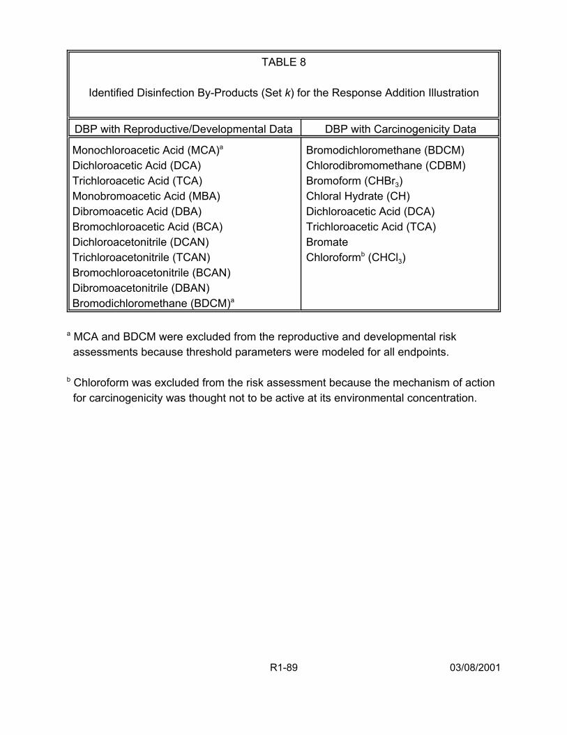
TABLE 8
Identified Disinfection By-Products (Set k) for the Response Addition Illustration
DBP with Reproductive/Developmental Data DBP with Carcinogenicity Data
Monochloroacetic Acid (MCA)a
Dichloroacetic Acid (DCA) Trichloroacetic Acid (TCA) Monobromoacetic Acid (MBA) Dibromoacetic Acid (DBA) Bromochloroacetic Acid (BCA) Dichloroacetonitrile (DCAN) Trichloroacetonitrile (TCAN) Bromochloroacetonitrile (BCAN) Dibromoacetonitrile (DBAN) Bromodichloromethane (BDCM)a
Bromodichloromethane (BDCM) Chlorodibromomethane (CDBM) Bromoform (CHBr3) Chloral Hydrate (CH) Dichloroacetic Acid (DCA) Trichloroacetic Acid (TCA) Bromate Chloroformb (CHCl3)
a MCA and BDCM were excluded from the reproductive and developmental risk assessments because threshold parameters were modeled for all endpoints.
b Chloroform was excluded from the risk assessment because the mechanism of action for carcinogenicity was thought not to be active at its environmental concentration.
R1-89 03/08/2001
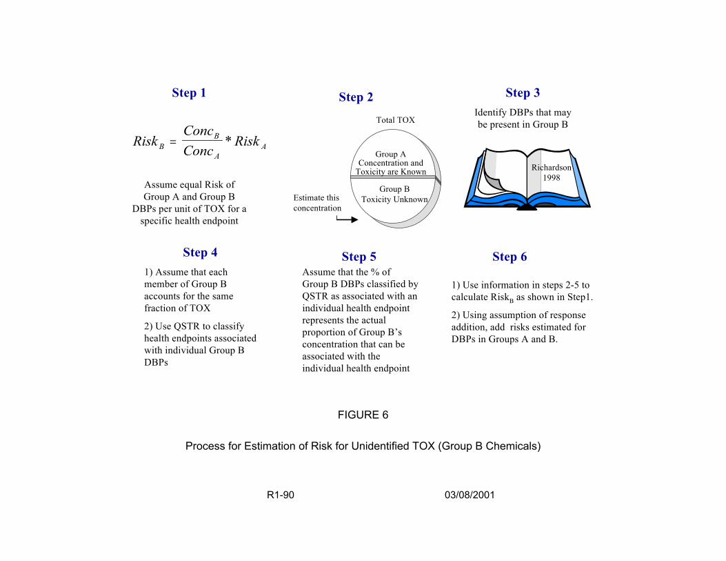
Step 1 Step 2
Total TOX ConcBRiskB = Conc
* Risk A A
Assume equal Risk of Group A and Group B
DBPs per unit of TOX for a specific health endpoint
Step 4 1) Assume that each member of Group B accounts for the same fraction of TOX
2) Use QSTR to classify health endpoints associated with individual Group B DBPs
Estimate this concentration
Group AConcentration and
Toxicity are Known
Group B Toxicity Unknown
Step 5 Assume that the % of Group B DBPs classified by QSTR as associated with an individual health endpoint represents the actual proportion of Group B’s concentration that can be associated with the individual health endpoint
FIGURE 6
Step 3 Identify DBPs that may be present in Group B
Richardson 1998
Step 6
1) Use information in steps 2-5 to calculate RiskB as shown in Step1.
2) Using assumption of response addition, add risks estimated for DBPs in Groups A and B.
Process for Estimation of Risk for Unidentified TOX (Group B Chemicals)
R1-90 03/08/2001

• Step 4. The QSTR model was used to classify each of the selected Group B DBPs as either associated with a health endpoint or not, resulting in the calculation of a percentage of Group B DBPs associated with the health endpoint. In the illustration, QSTR models in TOPKAT©
were used to assess the toxicity of each of the Group B DBPs (Moudgal et al., 2000). The fractions of Group B DBPs found to be associated with cancer and developmental toxicity were 58% and 42%, respectively, for the chlorination system and 55% and 56%, respectively, for the preozonation followed by chlorination system. Because TOPKAT© did not have a reproductive toxicity model, the developmental toxicity values were also used as surrogates for the fraction of Group B DBPs that may be associated with inducing reproductive toxicity.
• Step 5. The percentage of Group B DBPs associated with the health endpoint was extrapolated directly to estimate the proportion of the Group B organic halide concentration that could be associated with the health endpoint.
• Step 6. Using the ratio of Group B to Group A organic halide concentrations associated with the health endpoint of concern, the risk for the Group B DBPs was calculated as shown in Step 1.
The total endpoint-specific risk, using Equation 1, is the sum of the risks for the
identified DBPs (Group A), as calculated from known toxicity and measurement data,
and the unidentified DBPs (Group B), as estimated using Steps 1 through 6.
2.6.1. Development of Distributions of Risks. For the illustration, a two-stage Monte
Carlo analysis was performed, as shown in Figure 7, to calculate distributions of DBP
mixture risk using Equation 1. Input distributions were developed to quantify variability
(heterogeneity) in the population tap water consumption rates (Y), (i.e., the range of
plausible risks resulting from differences among members of the population) and to
quantify uncertainty (i.e., the range of plausible risks for each individual corresponding
to alternative plausible assumptions) for DBP concentration data (Ci) and DBP toxicity
R1-91 03/08/2001
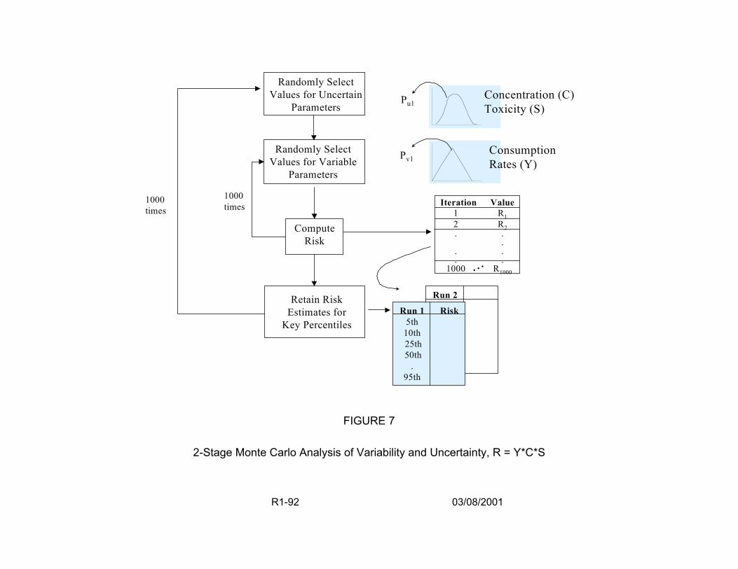
R1-92 03/08/2001
1000 times
FIGURE 7
2-Stage Monte Carlo Analysis of Variability and Uncertainty, R = Y*C*S
Run 2
Randomly Select Values for Uncertain
Parameters
Randomly Select Values for Variable
Parameters
Retain Risk Estimates for
Key Percentiles
Compute Risk
Pu1
Pv1
Iteration Value 1 1 2 2 .
. . .
1000 R1000
Run 1 Risk 5th
10th 25th 50th
. 95th
...
1000 times
Concentration (C) Toxicity (S)
Consumption Rates (Y)
RR.
.
.
estimates (Si). The result of such an analysis is the development of risk distributions, as
shown in Figure 8, that reflect variability on the X-axis and uncertainty on the Y-axis.
Variability was quantified by holding uncertain assumptions fixed and computing
risk estimates corresponding to different values for parameters that vary among
members of the population. Uncertainty was quantified by computing risk for several
“representative” members of the population, such as the median individual and the 95th
percentile individual. Values for uncertain parameters (e.g., cancer slope factors and
DBP concentrations) were randomly selected and held constant, and then 1000 sets of
values for the variable parameters (e.g., water consumption, L-kg/day) were randomly
drawn (corresponding to 1000 iterations of the inner loop) and used to compute 1000
estimates of risk. After ranking the 1000 risk estimates from the inner loop, some key
population summary statistics estimates (i.e., 5th, 10th, 25th, 50th, 75th, 90th, and 95th
percentiles) were retained (Figure 8). The simulation then proceeded to the next
iteration of the outer loop, selecting new random values for the uncertain parameters
and then executing 1000 new iterations of the inner loop. The outer loop was ultimately
executed 1000 times, yielding 1000 estimates of each of the key population summary
statistic risk estimates.
2.6.1.1. Tap Water Consumption (Y) — DBP exposure was assumed to be a
function of total tap water consumed. All water from the household tap consumed
directly as a beverage or used to prepare foods and beverages was considered tap
water. The studies of Ershow and Cantor (1989) of the U.S. population and the
Canadian Ministry of National Health and Welfare (1981), presented in U.S. EPA
R1-93 03/08/2001
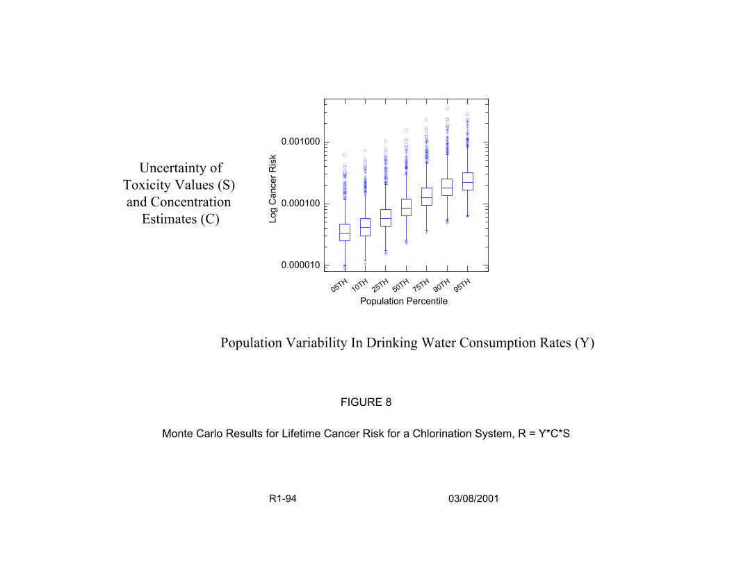
0.001000
Uncertainty of Toxicity Values (S) and Concentration
Estimates (C) Log
Can
cer R
isk
0.000100
0.000010
H1 H
2 H5 H
7 H9 H
9 H50 T T0 T5 T0 T5 T0 T5
Population Percentile
Population Variability In Drinking Water Consumption Rates (Y)
FIGURE 8
Monte Carlo Results for Lifetime Cancer Risk for a Chlorination System, R = Y*C*S
R1-94 03/08/2001
Exposure Factors Handbook (1997b) were used to derive consumption estimates. The
illustration approach quantified tap water consumption by fitting lognormal distributions
to age-specific intake data for the U.S. population developed by U.S. EPA (1997b),
based on Ershow and Cantor (1989) and shown in Table 9. The water consumption of
some subpopulations was evaluated and found not to differ from the general population
estimates. The illustration did not, however, evaluate exposure routes other than oral,
compare differences in DBP exposures from heated vs. unheated tap water, or account
for potential changes in consumption patterns (e.g., increased use of bottled water)
since the time of data collection by Ershow and Cantor (1989).
2.6.1.2. DBP Concentrations in Drinking Water (Ci) — Concentration data (in
µg/L) for individual DBPs in the illustration (one with chlorination only and one with
chlorination following pre-ozonation) were adapted from a paper by Miltner et al.,
(1990), resulting from a study in which Ohio River water was treated in a pilot plant and
then subjected to a simulated distribution system for each of the treatment trains. Table
10 lists the resulting concentration data used in the case study. These data are slightly
different from the Miltner et al. (1990) paper because the means and confidence limits
were recalculated from the sampling data assuming a normal distribution and
substituting half the detection limit for non-detects instead of zero, which was used in
the original publication. The notable exception is that the concentrations for bromate
were not sampled at the time of the study and have been estimated using more recent
information.
R1-95 03/08/2001
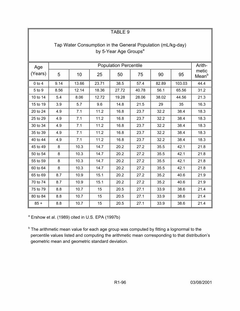
R1-96
03/08/2001
TABLE 9
Tap Water Consumption in the General Population (mL/kg-day) by 5-Year Age Groupsa
Population Percentile Age
(Years) 5 10 25 50 75 90 95
Arith-metic Meanb
0 to 4 9.14 13.66 23.71 38.5 57.4 82.89 103.03 44.4
5 to 9 8.56 12.14 18.36 27.72 40.78 56.1 65.56 31.2
10 to 14 5.4 8.06 12.72 19.28 28.06 38.02 44.56 21.3
15 to 19 3.9 5.7 9.6 14.8 21.5 29 35 16.3
20 to 24 4.9 7.1 11.2 16.8 23.7 32.2 38.4 18.3
25 to 29 4.9 7.1 11.2 16.8 23.7 32.2 38.4 18.3
30 to 34 4.9 7.1 11.2 16.8 23.7 32.2 38.4 18.3
35 to 39 4.9 7.1 11.2 16.8 23.7 32.2 38.4 18.3
40 to 44 4.9 7.1 11.2 16.8 23.7 32.2 38.4 18.3
45 to 49 8 10.3 14.7 20.2 27.2 35.5 42.1 21.8
50 to 54 8 10.3 14.7 20.2 27.2 35.5 42.1 21.8
55 to 59 8 10.3 14.7 20.2 27.2 35.5 42.1 21.8
60 to 64 8 10.3 14.7 20.2 27.2 35.5 42.1 21.8
65 to 69 8.7 10.9 15.1 20.2 27.2 35.2 40.6 21.9
70 to 74 8.7 10.9 15.1 20.2 27.2 35.2 40.6 21.9
75 to 79 8.8 10.7 15 20.5 27.1 33.9 38.6 21.4
80 to 84 8.8 10.7 15 20.5 27.1 33.9 38.6 21.4
85 + 8.8 10.7 15 20.5 27.1 33.9 38.6 21.4
a Ershow et al. (1989) cited in U.S. EPA (1997b) b The arithmetic mean value for each age group was computed by fitting a lognormal to the percentile values listed and computing the arithmetic mean corresponding to that distribution’s geometric mean and geometric standard deviation.
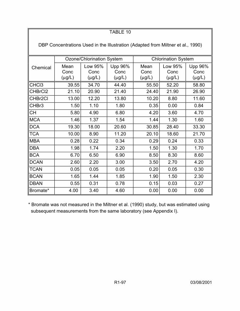
TABLE 10
DBP Concentrations Used in the Illustration (Adapted from Miltner et al., 1990)
Ozone/Chlorination System Chlorination System
Chemical Mean Conc (:g/L)
Low 95% Conc (:g/L)
Upp 96% Conc (:g/L)
Mean Conc (:g/L)
Low 95% Conc (:g/L)
Upp 96% Conc (:g/L)
CHCl3 39.55 34.70 44.40 55.50 52.20 58.80CHBrCl2 21.10 20.90 21.40 24.40 21.90 26.90 CHBr2Cl 13.00 12.20 13.80 10.20 8.80 11.60 CHBr3 1.50 1.10 1.80 0.35 0.00 0.84 CH 5.80 4.90 6.80 4.20 3.60 4.70 MCA 1.46 1.37 1.54 1.44 1.30 1.60 DCA 19.30 18.00 20.60 30.85 28.40 33.30 TCA 10.00 8.90 11.20 20.10 18.60 21.70 MBA 0.28 0.22 0.34 0.29 0.24 0.33 DBA 1.98 1.74 2.20 1.50 1.30 1.70 BCA 6.70 6.50 6.90 8.50 8.30 8.60 DCAN 2.60 2.20 3.00 3.50 2.70 4.20 TCAN 0.05 0.05 0.05 0.20 0.05 0.30 BCAN 1.65 1.44 1.85 1.90 1.50 2.30 DBAN 0.55 0.31 0.78 0.15 0.03 0.27 Bromate* 4.00 3.40 4.60 0.00 0.00 0.00 * Bromate was not measured in the Miltner et al. (1990) study, but was estimated using subsequent measurements from the same laboratory (see Appendix I).
R1-97 03/08/2001

2.6.1.3. Toxicity Estimates (Si) — The toxicity estimate for each identified DBP
was assumed to be lognormal with a geometric mean equal to the 50th percentile and
95th percentile values, as shown for cancer slope factors in Table 11. Although the
confidence intervals reported for toxicity estimates that were fit using maximum
likelihood techniques are theoretically normal. However, the relative magnitude of the
50th and 95th percentile values of the slope factors for many compounds, along with the
constraint that the slope factor must be non-negative, indicates that the true confidence
intervals must be skewed to the right. The lognormal distribution was used to
approximate this skew.
All dose-response modeling was performed using a linearized multistage
procedure, with a threshold parameter included in the model for the developmental and
reproductive endpoints. In the illustrative example, carcinogenicity dose-response data
were selected based on expert evaluations of the toxicology literature (i.e., Agency
reviews [U.S. EPA, 2000b; Bull and Kopfler, 1991]) and used in the response addition
procedure to estimate human health risks (see Section 4.3.1. of Appendix I). For
cancer, each identified DBP’s dose-response was assumed to be linear with no
threshold for each DBP identified as a carcinogen through in vivo toxicologic
evaluations. The exception to this was chloroform, whose mechanism of action for
cancer was not considered to be active at the exposure concentrations in the Miltner et
al. (1990) study.
In the illustrative example (see Section 4.3.2., Appendix I), a careful toxicological
review was done for each DBP identified in the in vivo toxicology literature to evaluate
R1-98 03/08/2001
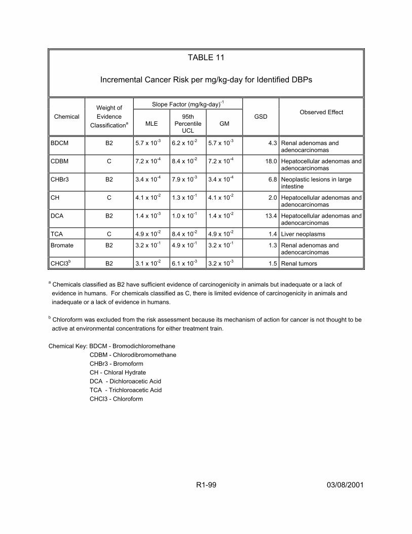
TABLE 11
Incremental Cancer Risk per mg/kg-day for Identified DBPs
Slope Factor (mg/kg-day)-1
Chemical Weight of Evidence
Classificationa MLE 95th
Percentile UCL
GM GSD
Observed Effect
BDCM B2 5.7 x 10⁻³ 6.2 x 10⁻² 5.7 x 10⁻³ 4.3 Renal adenomas and adenocarcinomas
CDBM C 7.2 x 10⁻⁴ 8.4 x 10⁻² 7.2 x 10⁻⁴ 18.0 Hepatocellular adenomas and adenocarcinomas
CHBr3 B2 3.4 x 10⁻⁴ 7.9 x 10⁻³ 3.4 x 10⁻⁴ 6.8 Neoplastic lesions in large intestine
CH C 4.1 x 10⁻² 1.3 x 10⁻¹ 4.1 x 10⁻² 2.0 Hepatocellular adenomas and adenocarcinomas
DCA B2 1.4 x 10⁻³ 1.0 x 10⁻¹ 1.4 x 10⁻² 13.4 Hepatocellular adenomas and adenocarcinomas
TCA C 4.9 x 10⁻² 8.4 x 10⁻² 4.9 x 10⁻² 1.4 Liver neoplasms
Bromate B2 3.2 x 10⁻¹ 4.9 x 10⁻¹ 3.2 x 10⁻¹ 1.3 Renal adenomas and adenocarcinomas
CHCl3b B2 3.1 x 10⁻² 6.1 x 10⁻³ 3.2 x 10⁻³ 1.5 Renal tumors
a Chemicals classified as B2 have sufficient evidence of carcinogenicity in animals but inadequate or a lack of evidence in humans. For chemicals classified as C, there is limited evidence of carcinogenicity in animals and inadequate or a lack of evidence in humans. b Chloroform was excluded from the risk assessment because its mechanism of action for cancer is not thought to be active at environmental concentrations for either treatment train. Chemical Key: BDCM - Bromodichloromethane CDBM - Chlorodibromomethane CHBr3 - Bromoform CH - Chloral Hydrate DCA - Dichloroacetic Acid TCA - Trichloroacetic Acid CHCl3 - Chloroform
R1-99 03/08/2001
the observed DBP dose-related developmental and reproductive effects (e.g.,
resorptions, fetal deaths, malformations, fetal weight, sperm abnormalities). Then, for
each DBP, all endpoints were individually modeled using a linearized multistage
procedure with a threshold parameter. For those dose-response data for which the
threshold parameter was not statistically significantly different from zero, the most
sensitive endpoint was selected for inclusion in the response addition procedure to
estimate human health risks. (In all cases in which the threshold parameter was
different from zero, the exposure concentrations were below the threshold estimate, so
risk was estimated to be zero.) To model continuous endpoints, the analysis first
converted them into quantal endpoints by designating a cutpoint in the upper tail of the
effect’s distribution in the control animal data. The cutpoint was selected to represent a
toxicologically adverse effect (see Appendix I).
2.6.1.4. Uncertainty Analysis — As discussed fully in Appendix I, the risk
estimates for each health effect (i.e., cancer and reproductive/developmental toxicity)
were quantified by combining exposure estimates with toxicity coefficients for the
identified DBPs and adding these to the risks estimated for the unidentified DBPs. It is
recognized that there is considerable uncertainty in these risk estimates because of
many factors. Following the generation of a distributions of plausible risks, additional
sensitivity and uncertainty analyses were performed. An analysis of the relationship
between the model input variables and the model output identified those variables that
had the greatest impact on the results. For each health condition (cancer,
developmental toxicity, and reproductive toxicity), the set of parameters having the
greatest influence on the determination of risk was identified by using linear regression
R1-100 03/08/2001
to model the population mean risk as a function of the uncertain parameters.
Uncertainty in the slope factor estimates accounted for the largest portion of the
parametric uncertainty in risk estimates for the cancer endpoints. However, the
concentration of unidentified total organic halide (TOX) DBP contributed the largest
portion of the parametric uncertainty in the developmental and reproductive toxicity
endpoints.
Not all of the sources of uncertainty, however, were quantified within the two-
stage Monte Carlo procedure. Some of these uncertainties were examined by
repeating the probabilistic analysis using different models, data sets or alternative
assumptions and comparing the results with the initial analysis. Such additional
analyses provided information on the reliability of the initial analysis and were useful in
planning new research activities. A summary of the results for the additional analyses
made in the illustration is presented below.
A. Exposure Uncertainties
1) The assumption that tap water ingestion dominates intake
2) The use of total tap water intake, rather than another estimate of tap water intake such as unheated tap water
The exposure assumption that ingestion dominates intake could be significant if
other routes of exposure result in much more efficient uptake or metabolism of the
DBPs. Total tap water intake as the relevant measure of exposure is unlikely to be
important. Although there is some speculation that heating tap water may remove some
of the volatile DBP, restricting attention to the intake of only unheated water affects the
R1-101 03/08/2001
estimate of risk by at most a factor of 2, indicating that this assumption is not a relatively
important source of uncertainty.
B. Toxicity Uncertainties
1) Use of QSAR to quantify the proportion of unidentified DBPs associated with a health endpoint
2) The assumption that the unidentified DBPs pose the same risk as the identified DBPs per concentration of organic halide
3) The assumption that the mechanism of action for chloroform carcinogenicity is not active at levels found in drinking water
4) Use of animal toxicology data to quantify the toxicity estimate or slope factor (Si), instead of epidemiologic data
5) The assumption that the slope factors (Si) are statistically independent
The proportion of unidentified DBPs associated with a health endpoint was
quantified using QSAR. The range of risks associated with the extreme alternative
assumptions of 0% or 100% generally spanned a factor of approximately 5 to 10,
suggesting that this assumption does not substantially contribute to uncertainty.
The assumption that the unidentified DBPs pose the same risk as the identified
DBPs was evaluated by assuming alternatively that the unidentified DBP pose only 50%
the risk as the identified DBPs per concentration, and that the unidentified DBPs pose
twice the risk as the identified DBPs per concentration. The results indicate that this
range of assumptions corresponds to a range of risk estimates spanning a factor of
approximately 5 to 10.
R1-102 03/08/2001
The assumption that chloroform’s mechanism of action for cancer is not active at
the levels in drinking water affects the overall risks by approximately 1.2 to 1.4, despite
the concentration data for chloroform (in this illustration) that show it is large and
exceeds that of many of the other DBPs. Whether chloroform is a carcinogen at
environmentally relevant exposure levels affects the cancer risk estimates for two
reasons. First, because the concentration of chloroform exceeds that of many other
DBPs, its potential contribution to carcinogenicity is substantial. The assumption of a
threshold dose-response for carcinogenicity removes its contribution from the risk
estimate. Second, because chloroform’s concentration is large compared to that of
other DBPs, its classification as a carcinogen affects the estimated risk associated with
exposure to unidentified DBPs. Specifically, if it is not classified as a carcinogen, its
potency is removed from the weighted average used as an estimate of the typical
potency of an unidentified DBPs. Because chloroform’s assumed potency is less than
the weighted average potency of the other identified DBPs, removing it from
consideration (by assuming it does not behave as a carcinogen at environmentally
relevant doses) increases the weighted average potency of the set of identified DBPs.
These two influences on risk work in opposite directions and hence, partially cancel
each other out.
Risk estimates computed under the assumption that for each health endpoint, the
slope factors are perfectly correlated, do not differ substantially from the risk estimates
computed under the assumption that these quantities are statistically independent. This
finding indicates that the assumption of statistical independence is not an important
source of uncertainty.
R1-103 03/08/2001
In place of the animal bioassay data used to quantify DBP carcinogenicity, the
epidemiology literature could be used. Calculations made using epidemiologic
information suggest a broad range of risks, ranging from zero to risks that may be
substantially larger than those determined from the animal data. Thus, the weak to
moderate findings for cancer using the epidemiologic data may be considered
important; the risk estimated from the animal studies could be an underestimate.
Because of these uncertainties, it is conceivable that the plausible range of risks from
exposure to the DBP mixtures is very broad and could include zero.
R1-104 03/08/2001
3. EPA’s MAIN CONCLUSIONS AND RECOMMENDATIONS BASED ON THE APRIL 1999 WORKSHOP
EPA held a workshop in April 1999 to examine the response addition illustration
and to advance the development of methodology to assess health risk for mixtures of
drinking water DBPs. The goal of the workshop was to assemble a multidisciplinary
group of scientists to formulate a range of possible approaches to solving this problem
and then provide guidance on the most practical and scientifically sound directions the
EPA should take to improve the risk assessment (see Charge to Participants, Attendees
in Report 2). Based on the results of this workshop, in this section, EPA recommends
certain issues for consideration regarding improvement of the DBP mixtures risk
assessment methodology. In Report 2 of this document are many discussions and
recommendations from workshop participants. Each of these was considered by EPA
within the context of the Agency’s previous experience with DBP mixtures risk
assessment and evaluated for scientific validity, feasibility of application in the near-
term, data availability, consistency with other Agency Guidelines and practices, and
relevance to risk assessment goals and regulatory needs. The recommendations
selected are presented in this section. They potentially have the most significant, near-
term impact on improving DBP mixtures risk assessment. Additionally, EPA identified a
number of longer term research needs; these are presented in Section 5 of this Report.
R1-105 03/08/2001
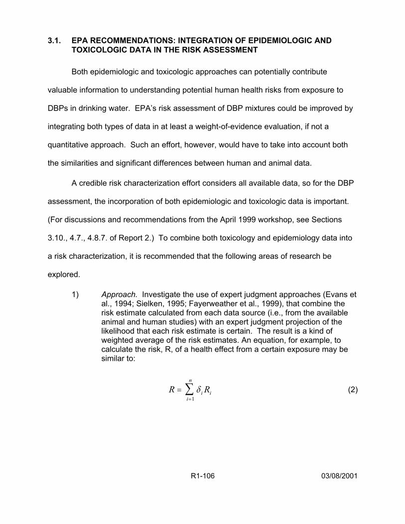
3.1. EPA RECOMMENDATIONS: INTEGRATION OF EPIDEMIOLOGIC AND TOXICOLOGIC DATA IN THE RISK ASSESSMENT
Both epidemiologic and toxicologic approaches can potentially contribute
valuable information to understanding potential human health risks from exposure to
DBPs in drinking water. EPA’s risk assessment of DBP mixtures could be improved by
integrating both types of data in at least a weight-of-evidence evaluation, if not a
quantitative approach. Such an effort, however, would have to take into account both
the similarities and significant differences between human and animal data.
A credible risk characterization effort considers all available data, so for the DBP
assessment, the incorporation of both epidemiologic and toxicologic data is important.
(For discussions and recommendations from the April 1999 workshop, see Sections
3.10., 4.7., 4.8.7. of Report 2.) To combine both toxicology and epidemiology data into
a risk characterization, it is recommended that the following areas of research be
explored.
1) Approach. Investigate the use of expert judgment approaches (Evans et al., 1994; Sielken, 1995; Fayerweather et al., 1999), that combine the risk estimate calculated from each data source (i.e., from the available animal and human studies) with an expert judgment projection of the likelihood that each risk estimate is certain. The result is a kind of weighted average of the risk estimates. An equation, for example, to calculate the risk, R, of a health effect from a certain exposure may be similar to:
n
R = ∑ δ i Ri (2) i=1
R1-106 03/08/2001
where:
n = the number of data sets available
* i = is an expert judgment weight of the certainty the risk estimate for that data set is correct; the sum of the * i for n risk estimates equals 1
Ri = the risk calculated for data set i.
Rationale. Each data set, deemed to be of adequate quality, is used to produce a quantitative risk estimate. Thus, when the choice of data set is unclear, an arbitrary decision is not required. Furthermore, some sense of the quality and appropriateness of each data set can be factored into the calculation using expert judgment. For DBP mixtures risk estimation, for which the epidemiologic data are important and the calculated risks are relatively large, but the associations are weak, this offers a way to influence the outcome of the risk estimation process that otherwise may default to only using the animal toxicology data, while acknowledging the uncertainties in the databases for both data sources. This approach also offers the opportunity to develop distributions of risks that may be useful for comparisons and risk ranking efforts.
2) Approach. Evaluate differences in biology, exposure (including internal dose), and dose-response between animals and humans including:
• Elucidating the underlying modes-of-action that result in the expression of different health effects within the same target organ systems between humans and experimental animals
• Considering sensitive subpopulations, such as pregnant females, that may (or may not) respond differently between animals and humans
• Evaluating the enormous differences across species and within human exposures relative to duration, DBP concentration levels, lifestyle factors, and activity patterns that affect contact
• Identifying differences in physiology, biochemistry, anatomy, and metabolic responses that may produce disparate health outcomes.
R1-107 03/08/2001
Rationale. Human DBP exposures are generally lower than those used in animal studies. For DBP exposures, the health effects observed in these two types of studies are not always exactly the same (e.g., mostly liver and kidney tumors are observed in animal bioassays of DBPs, and bladder, colon and rectal tumors are associated with chlorinated drinking water in some epidemiologic studies), although similar target systems may be involved for each. Dose dependence of such tumor sites resulting from differences in exposures between animal studies and the epidemiologic literature may also be a factor.
Also, animal studies are often conducted using different routes than those to which the human population is exposed. Route-to-route and high-to-low dose extrapolations of data should take into account differences in how the DBPs are metabolized and distributed in the body. For example, after the ingestion of low concentrations of DBPs, nearly complete metabolism occurs during the first pass through the liver, while the inhaled and dermally-absorbed compounds are distributed throughout the body prior to hepatic metabolism. By contrast, because of high doses in animal studies, there generally is incomplete metabolism of the compounds, even when ingested. Thus, careful evaluation of the factors that affect toxicity for both humans and animals and identification of the differences in these factors will improve future risk assessments.
3) Approach. Convene a “Blue Ribbon” panel to identify the important issues regarding better characterization of the uncertainties associated with interpreting the epidemiologic literature and how best to quantify the human health risks of cancer and exposure to drinking water disinfectants and by-products (see Section 4.7. of Report 2 for additional details). The general composition of the panel should include epidemiologists, toxicologists, and quantitative analysts who have experience in complex problem solving. The primary interest of the panel is to objectively evaluate current studies and analyses of their results, identify the uncertainties, and recommend ways to reduce these uncertainties. They would also oversee the implementation of projects and tasks specifically designed to address the relevant issues.
Rationale. Both epidemiologic and toxicologic approaches contribute valuable information to the risk assessment process, but difficulties occur in incorporating epidemiologic results into the quantitative risk assessment. Better characterization of the uncertainties associated with the underlying epidemiologic literature is needed. When attempting to quantify human health risks, it should be recognized that available epidemiologic data are insufficient to establish a causal association
R1-108 03/08/2001
between DBP and cancer or reproductive risks. Epidemiologists and toxicologists express confusion about how to interpret study findings because of inherent differences in the design, execution, and analysis of the studies. Of particular concern are the non-comparability of the water exposures studied, methodological differences among the studies, internally inconsistent findings within studies, and the lack of consensus regarding causality for bladder, colon, and rectal cancers. The literature on reproductive and developmental effects is currently too sparse to use for quantitative risk assessment. One problem in attempting to interpret epidemiologic findings is incompletely presented dose-response information. Use of continuous data (where available) improves both the sensitivity and the power of the analyses.
3.2. IMPROVEMENTS IN EXPOSURE CHARACTERIZATION
In developing DBP exposure estimates, comprehensive exposure models should
be developed. These should incorporate the range of individual DBP concentrations at
both the treatment plant and within the distribution system over the etiologically relevant
time period; location and time spent in the distribution system; differences in the mixture
of DBPs during the exposure period caused by changes in water sources or treatment
practices; water use and consumption patterns that may affect ingestion, inhalation and
dermal exposures; other human behavioral activities or characteristics that may affect
exposure; and household/workplace characteristics. (For discussions and
recommendations from the April 1999 workshop, see Sections 3.4., 3.5., 3.6., 4.1. and
4.8.1. of Report 2.) Recommendations for improving the exposure characterization
include:
1) Approach. Develop better concentration data on DBPs in finished drinking water throughout the distribution system. Use data from the Information Collection Rule (ICR) as a source of distributional data on concentrations of THMs, HAAs, bromate, and aldehydes in water systems throughout the United States.
R1-109 03/08/2001

Rationale. These data help characterize DBP mixture exposures representative of specific source waters and drinking water treatment scenarios, including measures of seasonal fluctuations and variance in concentration data across geographic regions of the United States. It may be noted, however, that the limited number of samples within any system indicates that the full extent of the variability will likely not be captured by the ICR data.
2) Approach. Develop models that include multi-route exposures (i.e., oral, dermal and inhalation) when conducting risk assessments for DBPs. Consider the form in which consumption occurs (e.g., if water is heated before consumption, volatile organic compounds are driven off; thermally unstable compounds decrease; the concentration of non-volatile compounds may be increased because of water evaporation and volume reduction; inhalation exposures to the volatile compounds may be increased).
Rationale. DBPs have been measured in tap water and indoor air; some DBPs in tap water (e.g., chloroform) volatilize through heating during cooking, showering, etc. (e.g., Olin, 1999; Weisel and Chen, 1994; Giardino and Andelman, 1996). As a result, DBP exposures can occur through ingestion, inhalation, and dermal absorption. The inhalation exposure for volatile DBPs and dermal exposure to highly lipophilic DBPs can result in exposures equivalent to ingestion for median water uses. Thus when comparing risks from different water sources and treatment practices, which may result in different DBPs and concentrations, it is critical to include all exposure routes.
3) Approach. Recognize the etiologically-relevant exposure period, that is, the time frame over which exposure should be evaluated, and use this information in assessing risks.
Rationale. To evaluate the appropriate time period, it is necessary to consider the endpoint of interest: for acute effects (including reproductive or developmental), peak or average daily exposure may be needed, whereas for cancer, annual or integrated, longer-term exposure estimates may be required. A second consideration is to determine how the time frame over which exposures are expected to occur overlaps with the time frame(s) over which damage or effects occur at the molecular, cellular, tissue, or organ level. Both pharmacokinetic and pharmacodynamic studies are needed to address these temporal issues.
R1-110 03/08/2001

4) Approach. Develop tap water consumption and human activity pattern data for potentially sensitive subpopulations identified in epidemiology and toxicology studies that better characterize contact with the DBPs in different media. Potentially sensitive subpopulations include pregnant women, lactating women, and young children. Examine changes in water use and consumption patterns that occur during pregnancy and during the period of time in which women lactate (i.e., children obtain a larger quantity of milk from their mothers or wet nurses over time and then consumption decreases until nursing ceases.) For young children, examine the changes in DBP exposures that result from changes in activity patterns as they develop. Dermal exposures in newborns should be examined. Both mathematical models and biomarkers could be used in such evaluations.
Rationale. Data and models exist that can be used for this effort (e.g., tap water consumption for the general population and for pregnant women are available [U.S. EPA, 1997b]). Mathematical exposure models exist for use in risk assessments (e.g., Olin, 1999) based on physical/chemical properties of DBPs in water and assumptions concerning human activity patterns, as well as air exchange rates in buildings and room dimensions (ILSI, 1998). Studies of U.S. human activity patterns, such as tap water consumption distributions (including heated tap water consumption) and showering and bathing frequency and duration distributions, provide contact rates for important exposure media (U.S. EPA, 1997b). These data can be aggregated and used in the exposure assessment to estimate DBP contact rates for the three primary exposure routes.
5) Approach. Develop of additional mathematical models to predict the formation of DBPs similar to formation model for individual THMs developed by Clark and Sivaganesan (1998). DBPs of interest would include the HAAs , HANs, and chlopicrin.
Rationale. These data will help characterize DBP concentrations in the distribution system and provide additional data on the variations in levels of various DBPs. These variations depend upon the source waters and drinking water treatment systems considered and should include estimates of seasonal fluctuations and variance in concentration data across geographic regions of the United States.
R1-111 03/08/2001
3.3. ACCOUNTING FOR POTENTIAL TOXICITY OF UNIDENTIFIED DBPs
The DBP mixtures risk assessment should address the complex mixture in
addition to those chemicals routinely identified. It should also determine if exposures to
the unidentified compounds are of toxicologic concern. (For discussions and
recommendations from the April 1999 workshop, see Sections 4.2. and 4.8.2. of Report
2.) Thus, to improve the methodology for estimating risks that incorporates information
on the unidentified chemicals, the following recommendations are made:
1) Approach. Evaluate the assumption made in the illustrative example that the DBP mixture risks for Groups A and B are equal, per concentration of organic halide material. An initial evaluation of this assumption could be performed by assembling distributions of easily available data, such as LD50s, for each Group (where Group B chemicals must be identified using existing laboratory data) and comparing them for similar central tendency estimates and variability. LD50s can be derived by modeling experimental animal data or estimated using QSTR models.
Rationale. In the uncertainty analysis for the illustration, the assumption that the unidentified DBP pose the same risk per concentration as the identified DBP was evaluated by assuming alternatively that the unidentified DBP pose only 50% the risk as the identified DBP per concentration, and that the unidentified DBP pose twice the risk as the identified DBP per concentration. The results indicated that this range of assumptions corresponds to a range of risk estimates spanning a factor of approximately 5 to 10, which may be a significant difference depending on the severity of the effect being evaluated. Research to examine this assumption will reduce the uncertainty in this calculation.
2) Approach. Improve the chemical characterization of Groups B and C. One approach to this problem is to solicit the opinions of expert organic chemists who work in the analytical field as to the types of compounds comprising Groups B and C. Some of this work has already occurred through two workshops held in 1998 (see Appendix R1-A) and 2000 (for summary, see U.S. EPA, 2001).
Rationale. It is likely that the non-halogenated compounds comprising Groups A, B and C differ substantially. These differences are likely to
R1-112 03/08/2001
include molecular weight, functional molecular subunits, and number of halogens. Although formed through the same process, compounds in Group C may be quite different than DBPs comprising Groups A and B. It is important to examine modes-of-action associated with these agents as well as target organ toxicity and interaction effects. For example, formaldehyde is a likely component of Group C and is classified on EPA’s IRIS system as a probable human carcinogen; there is also an RfD based on histopathological changes in the intestinal tract.
3) Approach. Once a set of chemicals is selected to represent the Group B and C DBPs, QSTR models can be used to estimate their toxicity. Improvements can be made in this process by using alternative QSTR models:
• Use various QSTR models to provide more confidence in the toxicity predictions. Such an effort may yield various conflicting predictions, so that multiple “answers” are provided for analysis. However, this information could be examined as a body of data and considered under a weight of evidence scheme; multiple “answers” could be examined by expert judgment. One important distinction among models that may explain different “answers” is to consider whether the models are asking equivalent questions that will provide directly comparable information.
• Examine and estimate the misclassification errors for the various QSTR models used.
• Examine the range of predictions from various QSTR models and make risk predictions on that basis, e.g., by using zero as the lower bound and predicting the upper bound by assuming a worst case.
Rationale. The use of QSTR modeling of toxicity carries with it a degree of uncertainty that must be acknowledged and estimated. In the illustration, only one model was applied to the Group B DBPs to estimate the proportion of the unidentified TOX that could be associated with a given health endpoint. The range of risks associated with the extreme alternative assumptions of 0% or 100% generally spanned a factor of approximately 5 to 10. Although this is a reasonable range for this illustration, the range may be significantly different depending on the source water characteristics and treatment trains being examined. Research to examine this assumption will reduce the uncertainty in this calculation.
R1-113 03/08/2001
4) Approach. Perform a statistical evaluation of the certainty that chemicals are indeed present in the DBP mixture. When toxicity data on such chemicals are then used in the risk assessment, the likelihood that the compounds are truly present in the DBP mixture can be used as a weighting factor in the actual risk estimation or taken into account in the uncertainty analysis.
Rationale. The illustration gives equal weight to the risks estimated for the Group A and B DBPs, despite the fact the we are certain the Group A DBPs are present and only estimate that the Group B DBPs are present. Furthermore, within the Group B DBPs, there is a range of uncertainty because, for example, some Group B DBPs are clearly formed by the disinfection process, where others are suspected of being formed by the analytical chemistry methods themselves. Similar issues exist for the Group C DBPs.
5) Approach. Evaluate experimental and environmental DBP mixtures for sufficient similarity.
Rationale. Because of the variability in DBP mixtures, development of statistical and toxicologic criteria to evaluate the concept of sufficient similarity among DBP mixtures is potentially useful in comparing the relative risks posed by different types of DBPs, including the unknown fraction. For example, these types of approaches may prove valuable for comparing toxicities of and exposures to drinking waters with elevated brominated DBP levels to those containing elevated chlorinated DBP concentrations. They could also be used to make comparisons of exposure and toxicity among these two groups. Evaluation of the changes in concentrations of individual DBPs as the mixture travels through the distribution system (Clark and Sivaganesan, 1998) may also be useful in the comparisons of relative risks posed by different DBP mixtures.
3.4. RISK ASSESSMENT OF DEVELOPMENTAL AND REPRODUCTIVE EFFECTS
The assessment of developmental and reproductive risks can be improved by
using more appropriate dose-response models and evaluating the relationships
between the animal study endpoints and the human effects of concern. (For
discussions and recommendations from the April 1999 workshop, see Sections 3.2.,
3.3., 4.4. and 4.8.4. of Report 2.) The following recommendations are made:
R1-114 03/08/2001
1) Approach. To assess human risk from animal developmental toxicity data and account for possible intrafetal correlations, consider modeling the risk of any treatment-related developmental effect, rather than focusing on a specific effect. One method would be to aggregate the observed effects in the animal bioassay prior to running the chosen dose-response model. Another alternative is to model several endpoints together using a multivariate normal model.
Rationale. When only one data set (e.g., reduced fetal body weight in males) is finally selected out of several possibilities (e.g., visceral malformations, reduced fetal body weight in females, neural tube defects, etc.) for risk estimation, much information is lost. When it can be shown that modeling data sets together is both biologically and statistically reasonable (e.g., Stiteler et al., 1993; Vater et al., 1993; Velazquez et al., 1994), then efforts should be made to combine them in the modeling procedure.
2) Approach. A model such as the log-logistic model with underlying beta-binomial response variability is recommended for modeling a single quantal endpoint instead of the linearized multistage procedure used in the illustrative example.
Rationale. Such models account for the correlated nature of the results from typical developmental toxicity data sets (and from many reproductive toxicity data sets) and allow estimates of the fetal probabilities of response as a function of dose or exposure (and other covariates such as litter size). Usually, the modeling of developmental toxicity studies is limited by the fact that individual fetal data are not generally reported in the literature, requiring separate modeling of each endpoint. For the DBP analysis, however, such data are available. It is generally more appropriate to model individual embryo/fetal responses and control for litter effects, as opposed to litter-based summaries of response (e.g., litters with one or more affected fetuses are considered to be the responding litters) because more information is utilized in the analysis.
3) Approach. Explore different ways to model continuous endpoints. Instead of converting them into quantal endpoints by estimating a cutpoint beyond which effects are considered to be adverse, the analysis can model changes in the continuous variable itself (e.g., changes in mean birth weight) as a function of dose.
R1-115 03/08/2001
Rationale. Modeling the continuous variable itself allows the results to be linked to sequellae known or thought to be caused by changes in the continuous endpoint (e.g., adverse affects in the infant linked to low birth weight, or infertility linked to low sperm count), thus addressing the issue of relating effects observed in animal studies to human health effects. That is, the dose-response relationship for the continuous endpoint in animals could be projected to humans using a pharmacokinetic or allometric dose scaling procedure. Then, the implications for human risk using human data can be interpreted in the context of the continuous parameter (or its human analogue) to human clinical outcomes of concern. Such an analysis should, of course, be limited to parameters that have human analogues strongly related to adverse outcomes of concern. An advantage of the use of continuous intermediate parameters such as birth weights is that they are more amenable to epidemiologic study and measurement of population effects than the often rare quantal effects.
3.5. RISK ASSESSMENT OF CARCINOGENIC EFFECTS
To improve the mixtures risk assessment for carcinogenicity, additional research
is needed to provide better mechanistic information, epidemiologic exposure
characterizations and statistical modeling. (For discussions and recommendations from
the April 1999 workshop, see Sections 3.1., 3.10., 4.3. and 4.8.3. of Report 2.) The
following recommendations are made:
1) Approach. Improve statistical treatment of uncertainty in the cancer potency estimates, including animal-to-human extrapolation, selection of data set, cancer mechanisms and statistical sampling error. Methods exist for determining minimal estimates of uncertainty from the biological literature. For example, using the EPA’s upper confidence limit (UCL) estimate of risk (U.S. EPA, 2000b) as approximately a 95th percentile value (1.6449 standard deviations above the median) and representing uncertainties as log-normally distributed about a median estimate at about 0.072 times the EPA UCL, then the geometric standard deviation of the lognormal distribution representing uncertainties is 10 [log(.0724)/1.6449]
= 4.93 (Hattis and Goble, 1991; Hattis and Barlow, 1996; Hattis and Minkowitz, 1996). Work by Crouch (1996) and by Kodell et al. (1996) showed a GSD of 10.5-11. A scale can be used, then, to understand the difference between particular percentiles of log normal distributions (e.g.,
R1-116 03/08/2001
between the 5th and 95th percentile). This is one approach for showing central tendency and range of variability.
Rationale. Uncertainty/confidence distributions should be derived for cancer potency estimates for chemicals for which bioassay data exist. Methods in the literature can be used in the near term to provide better estimates of inter-individual variability in the population than the lognormal distributions used in the illustration.
2) Approach. Explore the assumption of independence versus similarity of carcinogenic modes of action across DBPs, which is critical to understanding if DBP risk estimates should be calculated using response addition (independence) or dose addition (similarity).
Rationale. The degree of similarity of mode of action that would negate the assumption of independence is not known and is likely to be dose-dependent. A particular toxic endpoint (e.g., liver tumors) might arise from many different mechanisms, which may or may not be independent.
3) Approach. Investigate the toxicology literature for each carcinogenic DBP and determine the likelihood that its mechanism-of-action for cancer is not active at environmental exposure levels.
Rationale. The mode of carcinogenic action of the DBPs is important in assessing whether the carcinogenic mode of action has a threshold. The question of response thresholds is critical primarily when significant extrapolation is needed from experimental or observational exposures to those of interest and because animal bioassay exposures are generally several orders of magnitude higher than human exposures to finished drinking water. Several important points of scientific uncertainty exist for the assessment of risk from threshold compounds.
4) Approach. Assess the quality of existing epidemiological studies, evaluating the likely DBP mix in the areas where the studies were conducted; determine the feasibility of developing water quality models to better estimate historical exposures to specific DBPs.
Rationale. A number of analytic epidemiological studies have been conducted to assess the cancer and reproductive or developmental risks that may be associated with consumption of chlorinated drinking water. Results differ among the studies conducted in various geographic areas. For studies with minimal sources of bias, these differences may be the result of possible differences in water exposures to various disinfection
R1-117 03/08/2001

by-products (DBPs) in the study areas. To decrease the uncertainties associated with the interpretation of this body of literature, it is necessary to develop better assessment methods for the DBPs and other exposures of interest. Results of such efforts could be used for possible re-analysis of recent, well-conducted analytic epidemiological studies.
3.6. ACCOUNTING FOR VARIABILITY AND UNCERTAINTY
The illustrative example addressed both variability and uncertainty (see Section
2.5. of Report 2 and Sections 2.2., 2.3., 2.4., 5.2., 5.3. of Appendix I). When available,
data were used to estimate distributions for parameters such as slope factors, DBP
concentrations and tap water consumption values. These distributions were then used
in a two-stage Monte Carlo analysis to generate distributions of risk estimates, and
uncertainty analyses were further developed to analyze the effect of uncertain
assumptions on the results.
3.6.1. Dose-Response Issues. Because a response addition approach is used to
estimate DBP mixtures risk in the illustrative example, slope factors, calculated using
the linearized multistage procedure, are one set of key parameters used to characterize
both the cancer and non-cancer risks. While this model has precedent for carcinogens,
the 1996 proposed Cancer Guidelines (U.S. EPA, 1996b) indicate other models should
be used if they are biologically more appropriate. Furthermore, model uncertainty is of
great concern for the non-cancer endpoints, as other models are available that account
for such variables as litter effects and the existence of thresholds. The following issues
and modeling techniques relative to accounting for variability and uncertainty in the
dose-response assessment can be applied to both the cancer and noncancer
endpoints. The caveat is that some other toxicity marker may be used in place of a
R1-118 03/08/2001

slope factor in future analyses, particularly for the noncancer endpoints. (For
discussions and recommendations from the April 1999 workshop, see Sections 3.7.,
4.6. and 4.8.6. of Report 2.)
1) Approach. Use data comparing potency in animals and humans for a generic set of chemicals to quantify the distribution of plausible human potency estimates associated with the DBP-potency estimates inferred from the animal toxicity data sets.
Rationale. Some work has been done on this for the cancer endpoint (see Allen et al., 1988, 1998; Shipp et al., 1989). In the workshop, it was demonstrated that the distribution of human cancer potency estimates corresponding to a slope-factor estimate inferred from an animal toxicity data set can be characterized as lognormal with a GSD of approximately 10 (see Section 3.1. of Report 2 of this document).
2) Approach. Use a Monte Carlo simulation or bootstrapping techniques to develop human slope factor distributions. When determining the value of a human slope factor to use for a set of simulations, take the animal-based slope factor estimate (which itself could be sampled from the distribution representing its stochastic uncertainty) and then sample from a distribution of human inter-individual sensitivities developed for the endpoint of interest (e.g., for cancer, a lognormal distribution having a mean equal to that animal-based estimate and a GSD of 10).
Rationale. In the illustrative example, the slope factors are treated as uncertain values that are input as lognormal distributions into the Monte Carlo procedure to determine uncertainty and variability associated with the risk estimates. The estimates of these slope factors can be improved by using real data to determine the shape and parameters of the distribution.
3) Approach. Consider both data set uncertainty and model uncertainty in any risk characterizations.
Rationale. Both the current approach and the bootstrapping method described above use a single animal data set and require the choice of a particular dose-response model. Both of these choices affect the uncertainty of the distribution produced. For many of the more common DBPs, multiple (animal) data sets exist that provide alternative slope factor estimates, and in some cases, studies exist in which no adverse
R1-119 03/08/2001

effects were observed. A variety of dose-response models are available, several of which may provide an acceptable fit to a single data set, but may provide very different slope factor estimates, particularly when extrapolating into the low-dose region of the curve. Such uncertainties should be investigated and accounted for in the Monte Carlo analysis.
4) Approach. Use the expert judgment method described above (Section 3.1.) with Equation 2 to evaluate model uncertainty for each toxicologic or epidemiologic data set. Model each data set using all dose-response functions or other risk methods that are biologically plausible and statistically appropriate (e.g., demonstrates a statistically significant goodness-of-fit). Then, for a given data set, produce a weighted average of the risk estimates for the exposure of interest as described above.
Rationale. This approach provides an evaluation of model uncertainty. Experts can “compare” the results of independent models. This quality of each model can be factored into the model uncertainty analysis.
5) Approach. Characterize uncertainty in the hazard identification step when evaluating DBPs.
Rationale. This is a fundamental source of uncertainty whether relying on animal bioassays or epidemiologic studies. There are clearly differences between chemicals in the degree of certainty that they are indeed capable of causing health effects in humans, particularly at the low environmental exposure levels for DBPs. To be most useful, the uncertainty should be characterized quantitatively so it is reflected in the risk estimates that are compared.
3.6.2. Exposure Issues. Even at the most fundamental level, concentrations of some
of the DBPs are uncertain for any given treatment system simply because the identity of
those DBPs is unknown. Above and beyond this fundamental difficulty, there are
uncertainty and variability issues that need to be recognized in relation to both
concentration and subsequent exposures. Variability and uncertainty in the exposure
estimates can be improved by considering changes over time. (For discussions and
R1-120 03/08/2001
recommendations from the April 1999 workshop, see Sections 3.4., 3.5., 3.6., 4.1., 4.6.,
4.8.6. of Report 2.)
1) Approach. For tap water consumption data, derivation of a distribution for temporal variation should be investigated to provide information different from that representing inter-individual variations.
Rationale. Because tap water intake is one of the key parameters determining exposure (once a set of DBP concentrations is given), some care must be taken in interpreting and using the tap water intake data to derive distributions characterizing variability and/or uncertainty. Of particular concern here is the lack of differentiation between percentiles of consumption across individuals and percentiles across days of consumption. It is believed that the available consumption data (presented in Ershow and Cantor, 1989) were averaged over 3-day periods. Such information on temporal variation might be important when considering the impact of some noncancer endpoints, where a long-term average daily dose may not be the most appropriate determinant of response.
2) Approach. Characterize the variance and uncertainty in concentration data according to the time over which the assessment is made and the dimensions of the exposure area (e.g., one treatment plant, one region, national).
Rationale. Measurement error associated with collection of concentration data (for which there is substantial laboratory involvement) is likely to be a significant contributor to uncertainty. Also, seasonal variation in source water characteristics and geographic variation should be taken into account when appropriate for the scope of the assessment.
3.7. MIXTURES RISK CHARACTERIZATION METHODS
As detailed in Section 2.1.2., any risk characterization approach needs to
address the interconnected elements of the risk assessment paradigm that include
hazard identification, dose response assessment, exposure assessment and risk
characterization with an uncertainty analysis. Investigations are needed into how well
R1-121 03/08/2001
different risk characterization methods work with the DBP data. (For discussions and
recommendations from the April 1999 workshop, see Sections 3.8., 3.9., 3.10., 4.1., 4.5.
and 4.8.5. of Report 2.)
1) Approach. Evaluate multiple chemicals and multiple routes of exposure for several endpoints over time. The DBP mixture risk assessment should be approached using the principles of cumulative risk. Although cumulative risk is a fairly new area of research, the results of existing efforts can be used to apply cumulative risk assessment principles to DBP mixtures. Specifically, Agency efforts in this area include guidance on evaluating multiple pathways of exposure (U.S. EPA, 1999b), guidance on the health risk assessment of chemical mixtures (U.S. EPA, 1999c), and documentation on cumulative risk that will soon be available from the Office of Pesticides and from the National Center for Environmental Assessment’s Risk Assessment Forum.
Rationale. Drawing on points that have been made in Sections 3.1. to 3.4. of this document, it is clear that the risk assessment of DBPs is a multifaceted problem that includes population exposures to multiple chemicals over a lifetime. Data developed on inhalation and dermal exposures indicate that these pathways may contribute significant amounts of DBPs. Furthermore, it may be proposed that differences in risk estimates made from the epidemiologic data vs. the animal toxicity are different because the animals are not exposed via multiple routes and durations are too short as compared with human exposures.
2) Approach. Apply and compare several types of risk characterization methods to evaluate additivity, to include response-addition, relative potency factors (dose-addition), and proportional response addition.
Rationale. The use of risk characterization methods other than response addition may be important, for example, for developmental endpoints, when different DBPs affect development at the same stages or critical periods. For example, the haloacetic acids and haloacetonitriles that have been tested for developmental toxicity produce a spectrum of effects in the postimplantation period including postimplantation loss, depression of fetal body weight and crown-rump length, and visceral and skeletal malformations. Thus, for these DBPs, the critical periods appear to be similar, and mode of action may be considered as similar, so a dose addition approach would be more appropriate. However, when mode of action and timing of effects are unknown, a comparison of risk values under different assumptions offers a range of risk estimates
R1-122 03/08/2001

under additivity, which is important because synergistic or anatagonistic responses are not likely to occur at the low environmental levels at which DBPs occur.
R1-123 03/08/2001
4. CONCEPTUAL MODEL FOR A CUMULATIVE RISK APPROACH
As noted above, several different risk characterization methods have been
recommended for estimating DBP mixtures risk: response-addition, relative potency
factors and proportional response addition (Section 3.7.). Detailed examples are
available within this document for the DBP mixtures problem for the oral route only
using response addition (Appendix I) and proportional response addition (Section 3.8. of
Report 2). Although each of these approaches has its strengths, neither of these
examples accounts for 1) multiple routes of exposure, 2) any toxicologic similarity
among chemicals in the mixture (beyond target organ effects), and 3) temporal issues of
exposure.
Section 4.1. presents a conceptual model that accounts for multiple routes of
exposure over time and toxicologic similarity of the components. This approach will be
expanded in an NCEA report on the feasibility of performing cumulative risk
assessments for non-cancer and cancer endpoints for mixtures of drinking water
disinfection by-products via inhalation, dermal, and oral exposures; the projected
completion date of this feasibility report is 2001.
4.1. MODEL CONSIDERATIONS AND REQUIREMENTS
Currently, it is feasible to approach human health risks posed by DBPs as a
cumulative risk problem. The current effort (Appendix I) to quantify human cancer risk
from exposure to DBP mixtures using animal data from the oral route alone produces
risk estimates several orders of magnitude lower than those projected using positive
R1-124 03/08/2001

epidemiologic data on chlorinated drinking water exposures in the study population
(other epidemiologic data indicate that risks posed may be negligible). If one assumes
that DBP exposures cause human cancers and that the positive epidemiologic results
provide unbiased quantitative estimates of the cancer risk posed by chlorinated water
exposures, then the discrepancy between risk estimates from the toxicological data and
the positive epidemiologic studies requires explanation. Several reasons for the
discrepancy are postulated, including failure to accurately extrapolate dosimetry
between animals and humans; failure to account for contribution to risk from inhalation
and dermal exposure routes; and failure to integrate the data according to the level of
organization at which the effects were observed (e.g., population, target organ, cellular).
The goals of a cumulative risk assessment for DBPs build upon those of the
current DBP mixture risk assessment (Appendix I). The goals of a new methodology
would include:
• To develop a mixtures approach that incorporates the flexibility to integrate selected mixtures risk models based on an understanding of the mode-of -action
• To consider the temporal nature of DBP exposures and variability of human activity patterns; address and appropriately integrate exposures through the three routes of primary concern for environmental pollutants: ingestion, dermal, and inhalation
• To address the main endpoints of concern in the epidemiologic literature: developmental and reproductive effects and cancer
• To identify the “risk-relevant” components of DBP mixtures, this may include organic halides not measured individually as well as DBPs that are not halogenated
R1-125 03/08/2001
• To estimate risks for various drinking water treatment trains, reflecting differences in those DBPs formed and their concentrations over time in the distribution system
• To generate central tendency risk estimates along with their associated probability distributions; such distributions of risks are needed to appropriately reflect both the uncertainty and variability found in these data
• To identify specific measures that could be incorporated into future epidemiologic investigations to improve exposure classification
• To develop mixtures risk characterization approaches that can be used in the evaluation of causality.
4.2. CUMULATIVE RISK APPROACH
Three general approaches for addressing additivity associated with low doses
components of a chemical mixture exist (see Section 2.2.). Dose addition assumes the
mixture components share an MOA; thus, doses of individual components can be
added together after being appropriately scaled for relative potency. Response addition
assumes component risks for a given target organ or tissue can be added given the
components’ effects are toxicologically and statistically independent. Finally, effects
addition assumes health outcomes attributable to individual components can be added
together, assuming that the toxicodynamics are similar across components. To
incorporate MOA data into the risk assessment, a dose-addition approach is
investigated here.
MOA refers to a continuum describing the key events and processes starting
from the point of toxicant-cell interaction and leading to the onset of a health endpoint
(see Figure 9). The MOA may involve several levels of toxicologic analysis and
R1-126 03/08/2001

Exposure Effect
Internal Biologically Early Altered Exposure Dose Effective Biological Structure/ Clinical Prognostic
Dose Effect Function Disease Significance
Susceptibility
FIGURE 9
Biological Marker Components in Sequential Progression from Exposure to Disease
Source: Schulte (1989)
R1-127 03/08/2001
influence based on the structural hierarchy of animal bodies: intracellular, intercellular,
tissue, organ, organ system, whole organism. Less is known about MOA as contrasted
with the term mechanism-of-action, which implies a detailed molecular description of the
induction of a health effect (see Section 2.2.1.).
Both ILSI (1999) and Wilkinson et al. (2000) have documented the complexities
associated with assessing risks posed by chemical classes exhibiting a common MOA.
These reports describe a range of chemical mixture risk assessment methods that could
be applied to a set of pesticides that exhibit a shared MOA, the organophosphates
(OP). The potential utility of the hazard index approach (U.S. EPA, 1999c), a chemical
mixtures approach that requires dose response and exposure data for each component,
and a relative potency factors approach (detailed below) are presented in each.
Wilkinson and collaborators also detail a combined margin of exposure approach, which
is conceptually related and mathematically similar to the hazard index approach. The
ILSI report describes an exposure schematic that can combine exposure estimates for
inhalation, oral and dermal exposure routes; Olin (1999) also describes conceptually
similar approaches for assessing exposures to drinking water contaminants and details
additional exposure considerations for combining estimates from multiple exposure
routes. Wilkinson et al. (2000) and Rhomberg (1999) elucidate the temporal
considerations that impact an assessment of risks posed by multiple chemicals.
Specifically, they both conclude the internal dose of the components matters more than
the timing of the exposures.
Cumulative risk assessment, as used in this document, examines the potential
for increased risks by considering multiple chemical exposures through multiple routes
R1-128 03/08/2001
over multiple time frames. Cumulative risks are conjectured to occur under a number of
conditions:
• When exposures (through multiple routes) to a group of chemicals that act through a common mechanism of toxicity occur within a physiologically-relevant time frame
• When exposures occur (through multiple routes) to a group of chemicals that impact different parts of a pharmacodynamic pathway that lead to a toxic response given the temporal considerations of the impacts (e.g., repair processes)
• When risks of a toxic effect estimated for each component using the component’s dose-response curve at the exposure concentration are additive, given temporal considerations of the response
• When there are synergistic interaction effects associated with exposures to two different chemicals (or dose-additive chemical groups) that occur over a physiologically-relevant time frame.
The physiologic time frame can reflect the pharmacokinetics (PK) or the
pharmacodynamics (PD) associated with exposures to specific components of the
chemical mixture. PK is the study of the fate of chemicals in the body; it deals with
absorption, distribution, biotransformation, and elimination. PD is the study of
biochemical and physiological effects of chemicals and their mechanisms of action. The
PK depend on exposure routes and patterns (e.g., duration, magnitude, and frequency).
Although four conditions are listed previously in this section, only a cumulative risk
approach arising from exposures to groups of chemicals that act through a common
mechanism of toxicity within a physiologically-relevant time frame is described.
Figure 10 illustrates the decision processes that would be undertaken to apply
this approach. The decision diagram is presented from left to right, although some
R1-129 03/08/2001
steps may be interative. The initial step is to evaluate the MOA data for the components
of a chemical mixture. If the components share a common MOA, then it may be
possible to develop a cumulative relative potency factors approach. This assumes that
component data for individual exposure routes meet criteria established for
implementing an RPF approach; specifically, one component is well studied and has a
dose-response function available for the effect of interest, and it is reasonable to
conclude from available data on toxicity or chemical structure that all components share
a common MOA (U.S. EPA, 1999c). If the components do not meet the criteria, then
some other assessment approach should be considered.
The next step is to evaluate the exposure scenario. By which routes are
individuals exposed and over what time frames do these exposures occur? Three
exposure routes are typically considered when assessing risks posed by environmental
mixtures: dermal, oral, and inhalation. DBP exposures occur through all three routes.
Similarly, the time frame of DBP exposures is thought to be intermittent throughout the
period of time spent indoors. Concentrations of volatile DBPs (e.g., THMs) increase
when activities such as showering, cooking, and clothes washing occur. Dermal
exposures occur through activities such as bathing and hand washing, and oral
exposures occur through drinking water and consuming water in or on foods.
The next step is to assess the impact of absorption, distribution,
biotransformation, and elimination on the DBP components as they are absorbed
R1-130 03/08/2001
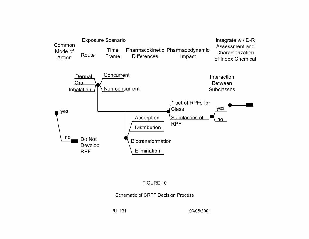
Exposure Scenario Common Mode of Time Action Route Frame
Pharmacodynamic Impact
Integrate w / D-R Assessment and Characterization
of Index Chemical Pharmacokinetic
Differences
Dermal Concurrent
Non-concurrent Oral
Inhalation
yes Absorption
Distribution
Biotransformation
Elimination
Do Not Develop RPF
no
FIGURE 10
Schematic of CRPF Decision Process
Interaction Between
Subclasses
1 set of RPFs for Class yes
Subclasses of no RPF
R1-131 03/08/2001
through the various exposure routes. Specifically, are there differences in internal dose
arising from the multiple route exposures? For example, when environmental
concentrations of chloroform are absorbed through the intestines, they appear to be
rapidly biotransformed in the liver. Inhaled chloroform is not biotransformed by the liver
as rapidly because it is not subjected to first pass effects.
The next step is to assess the PD differences. Do the components of the mixture
share a common MOA at environmental doses in the biological moiety(ies) of interest?
Can the MOA be plausibly linked to adverse health outcomes? If the data are generated
in laboratory animals, is there a comparable human MOA? If the components are
consistent across routes, PK, and PD properties, then it may logical to develop a single
set of RPFs for the compound class under evaluation. If they vary, then it may be
logical to split the class into two or more subclasses and pose the question as to the
type of interactions that exist between the classes. The final step is to develop an
equivalent index chemical concentration. This exposure assessment is then integrated
with the dose-response function of the index chemical to quantitatively estimate risk.
To implement this approach, it is critical to identify the assumptions made and
explain the basis for these assumptions. Typically, the data upon which to base many of
these decisions does not exist or may be difficult to interpret; expert judgement or
surrogate data may be used to facilitate decision making. In these cases, the
uncertainty introduced into the quantitative exposure assessment should be described.
The identification of uncertainty in mixtures risk assessments is critical (U.S. EPA, 1986,
1999c). The goal is to develop a transparent assessment, so that key assumptions can
be readily identified and evaluated.
R1-132 03/08/2001
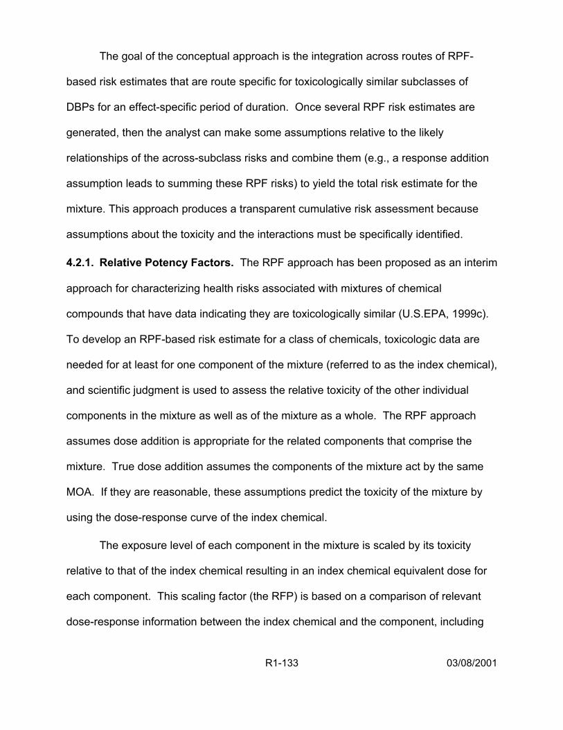
The goal of the conceptual approach is the integration across routes of RPF-
based risk estimates that are route specific for toxicologically similar subclasses of
DBPs for an effect-specific period of duration. Once several RPF risk estimates are
generated, then the analyst can make some assumptions relative to the likely
relationships of the across-subclass risks and combine them (e.g., a response addition
assumption leads to summing these RPF risks) to yield the total risk estimate for the
mixture. This approach produces a transparent cumulative risk assessment because
assumptions about the toxicity and the interactions must be specifically identified.
4.2.1. Relative Potency Factors. The RPF approach has been proposed as an interim
approach for characterizing health risks associated with mixtures of chemical
compounds that have data indicating they are toxicologically similar (U.S.EPA, 1999c).
To develop an RPF-based risk estimate for a class of chemicals, toxicologic data are
needed for at least for one component of the mixture (referred to as the index chemical),
and scientific judgment is used to assess the relative toxicity of the other individual
components in the mixture as well as of the mixture as a whole. The RPF approach
assumes dose addition is appropriate for the related components that comprise the
mixture. True dose addition assumes the components of the mixture act by the same
MOA. If they are reasonable, these assumptions predict the toxicity of the mixture by
using the dose-response curve of the index chemical.
The exposure level of each component in the mixture is scaled by its toxicity
relative to that of the index chemical resulting in an index chemical equivalent dose for
each component. This scaling factor (the RFP) is based on a comparison of relevant
dose-response information between the index chemical and the component, including
R1-133 03/08/2001
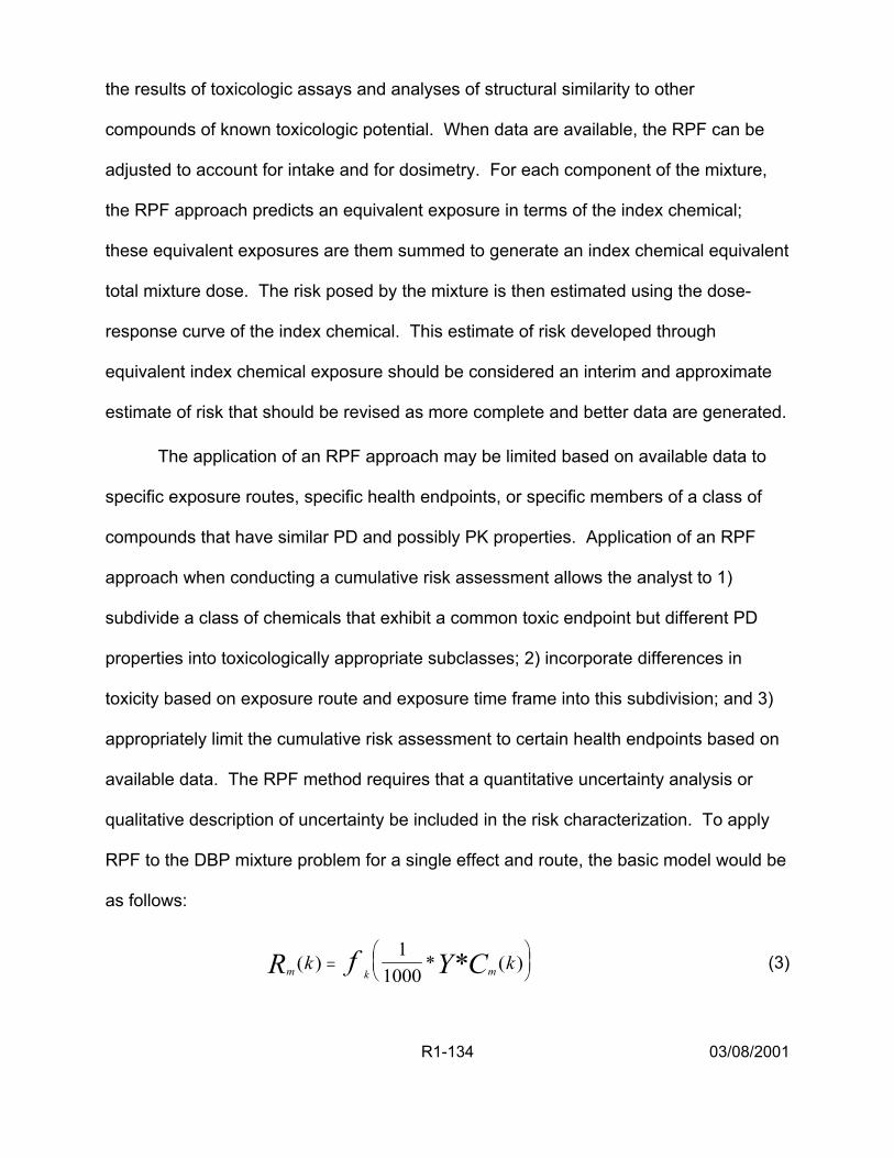
the results of toxicologic assays and analyses of structural similarity to other
compounds of known toxicologic potential. When data are available, the RPF can be
adjusted to account for intake and for dosimetry. For each component of the mixture,
the RPF approach predicts an equivalent exposure in terms of the index chemical;
these equivalent exposures are them summed to generate an index chemical equivalent
total mixture dose. The risk posed by the mixture is then estimated using the dose-
response curve of the index chemical. This estimate of risk developed through
equivalent index chemical exposure should be considered an interim and approximate
estimate of risk that should be revised as more complete and better data are generated.
The application of an RPF approach may be limited based on available data to
specific exposure routes, specific health endpoints, or specific members of a class of
compounds that have similar PD and possibly PK properties. Application of an RPF
approach when conducting a cumulative risk assessment allows the analyst to 1)
subdivide a class of chemicals that exhibit a common toxic endpoint but different PD
properties into toxicologically appropriate subclasses; 2) incorporate differences in
toxicity based on exposure route and exposure time frame into this subdivision; and 3)
appropriately limit the cumulative risk assessment to certain health endpoints based on
available data. The RPF method requires that a quantitative uncertainty analysis or
qualitative description of uncertainty be included in the risk characterization. To apply
RPF to the DBP mixture problem for a single effect and route, the basic model would be
as follows:
1k *Rm ( ) = f
k 1000
*Y Cm (k ) (3)
R1-134 03/08/2001

where:
Rm(k) = mixture risk for a given endpoint (unitless) as a function of an index chemical k
fk = dose response function of an index chemical k (a well-studied chemical in the mixture), requiring the 1/1000 conversion factor of mg to :g when dose units are mg/kg-day
Y = tap water intake rate (L/kg-day)
Cm(k) = concentration of the mixture in units of index chemical k (:g/L) [see m(k).]Equation 4 below for calculation of C
The RPF is based on dose addition, which carries with it the assumption of a
similar MOA for the mixture components, so each component can be considered a
dilution of the index chemical. To the extent that data are available, division of the
DBPs into subclasses could be performed by incorporating all relevant biological
information regarding toxicant-target interactions and response processes (e.g., it would
be important to distinguish between carcinogens that directly interact with and damage
DNA versus those that operate through epigenetic or nonmutagenic mechanisms such
as receptor-mediated pathways and hormonal or physiological disturbances).
The index chemical is likely to be chosen because it is a well studied chemical for
which the endpoint of interest has been observed, and its dose-response curve for that
endpoint is available. The concentrations of the other DBPs in the group then are
expressed as the index chemical by developing a scaling factor, the RPF. Then, the
total mixture dose is estimated as:
n
kCm ( ) = ∑ ( RPFi * Ci) (4) i =1
R1-135 03/08/2001

where:
Cm(k) = mixture exposure concentration expressed as the index chemical k (:g/L)
n = number of components in the mixture
RPFi = proportionality constant relative to the toxic potency of the index chemical, k, for the ith mixture component
Ci = measured concentration of the ith mixture component (:g/L).
Calculation of an RPFi involves making an estimate of relative potency for each
chemical compared with the index chemical. When data are available, dosimetric
adjustments, commensurate with level of effect observation and MOA, can be made
during this calculation to provide route-specific estimates of a cumulative internal dose
surrogate to adjust the RPFi.
Figure 11 presents a simple hypothetical RPF case for a single effect, route, and
duration. Chemical A1 is the index chemical. Equivalent concentrations of chemical
components A2 and A3 are developed and these are summed to estimate the index
chemical equivalent exposure for the simple mixture.
R1-136 03/08/2001
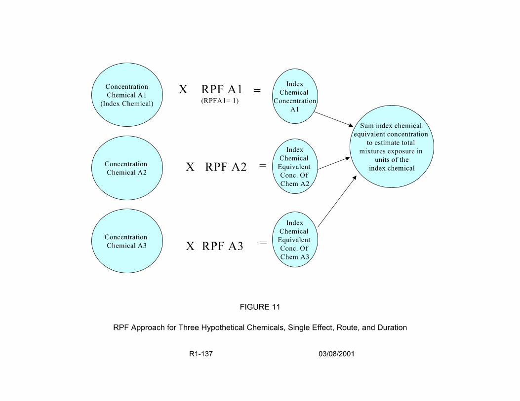
Concentration Chemical A1
(Index Chemical)
X RPF A1 = (RPFA1= 1)
Concentration Chemical A2 X RPF A2 =
Concentration Chemical A3 =X RPF A3
Sum index chemical equivalent concentration
to estimate total mixtures exposure in
units of the index chemical
Index Chemical
Equivalent Conc. Of Chem A2
Index Chemical
Equivalent Conc. Of Chem A3
Index Chemical
Concentration A1
FIGURE 11
RPF Approach for Three Hypothetical Chemicals, Single Effect, Route, and Duration
R1-137 03/08/2001

Figure 12 presents a simple hypothetical RPF case for a single effect over a
consistent time frame of exposure for two exposure routes. The oral exposure of
chemical A1 again serves as the index chemical for both oral exposures to chemicals
A2 and A3 and for exposures to chemical A1 through the inhalation route. Equivalent
concentrations of chemicals A2 , A3, and inhaled A1 are developed and these are
summed to estimate the index chemical equivalent exposure for the simple mixture.
The equivalent exposure is compared to the dose-response function of the index
chemical to estimate a risk. The assumptions or dosimetry data supporting the route-to-
route conversion for inhaled and oral chemical A1 would need to be clearly identified.
Tables 12 and 13 provide example calculations for a hypothetical subclass of five
DBPs that are liver carcinogens acting by the same MOA after oral ingestion. Table 12
illustrates some of the considerations related to data set evaluations, including data
availability and quality and differences in species and study durations. ED01 values are
estimated from each chemical’s critical study for use in the RPF approach; these should
be adjusted for dosimetry if enough data are available. The index chemical, k, exhibits
the best quality data set. For purposes of illustration, Table 13 shows a feasible set of
calculations that could be used to produce a risk estimate for this mixture using a RPF
approach. Ratios of the ED01 of the index chemical to the ith chemical’s ED01 provide an
RPFi for that chemical. The measured concentration, Ci, of the ith chemical is then
multiplied by its RPFi to adjust it to an index chemical equivalent concentration. In this
example, the risk for the mixture, Rm(k), is then estimated by multiplying the sum of
these equivalent concentrations, Cm(k), by the unit risk of the index chemical. The
R1-138 03/08/2001
Chemical A2 Oral
X RPFA2
Chemical A1 Inhalation X RPF Ai
Index Chemical A1 Equivalent
Concentration
Mixture Risk
Response
Chemical A1
=
Chemical A3 Oral
X RPFA3 Dose
FIGURE 12
RPF Approach for Three Hypothetical Chemicals, Two Exposure Routes
Index Chem. Chemical A1
Oral
R1-139 03/08/2001
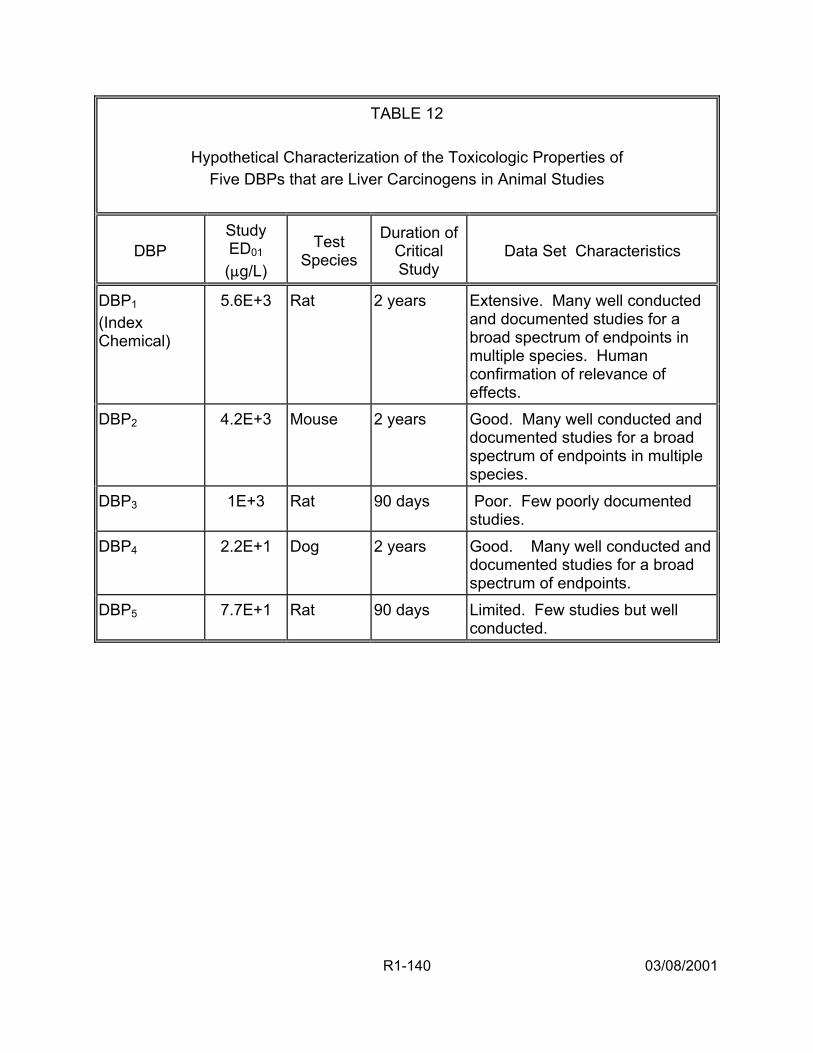
TABLE 12
Hypothetical Characterization of the Toxicologic Properties of Five DBPs that are Liver Carcinogens in Animal Studies
DBP Study ED01 (:g/L)
Test Species
Duration of Critical Study
Data Set Characteristics
DBP1 (Index Chemical)
5.6E+3 Rat Extensive. Many well conducted and documented studies for a broad spectrum of endpoints in multiple species. Human confirmation of relevance of effects.
DBP2 4.2E+3 Mouse 2 years Good. Many well conducted and documented studies for a broad spectrum of endpoints in multiple species.
DBP3 1E+3 Rat 90 days Poor. Few poorly documented studies.
DBP4 2.2E+1 Dog 2 years Good. Many well conducted and documented studies for a broad spectrum of endpoints.
DBP5 7.7E+1 Rat 90 days Limited. Few studies but well conducted.
2 years
R1-140 03/08/2001
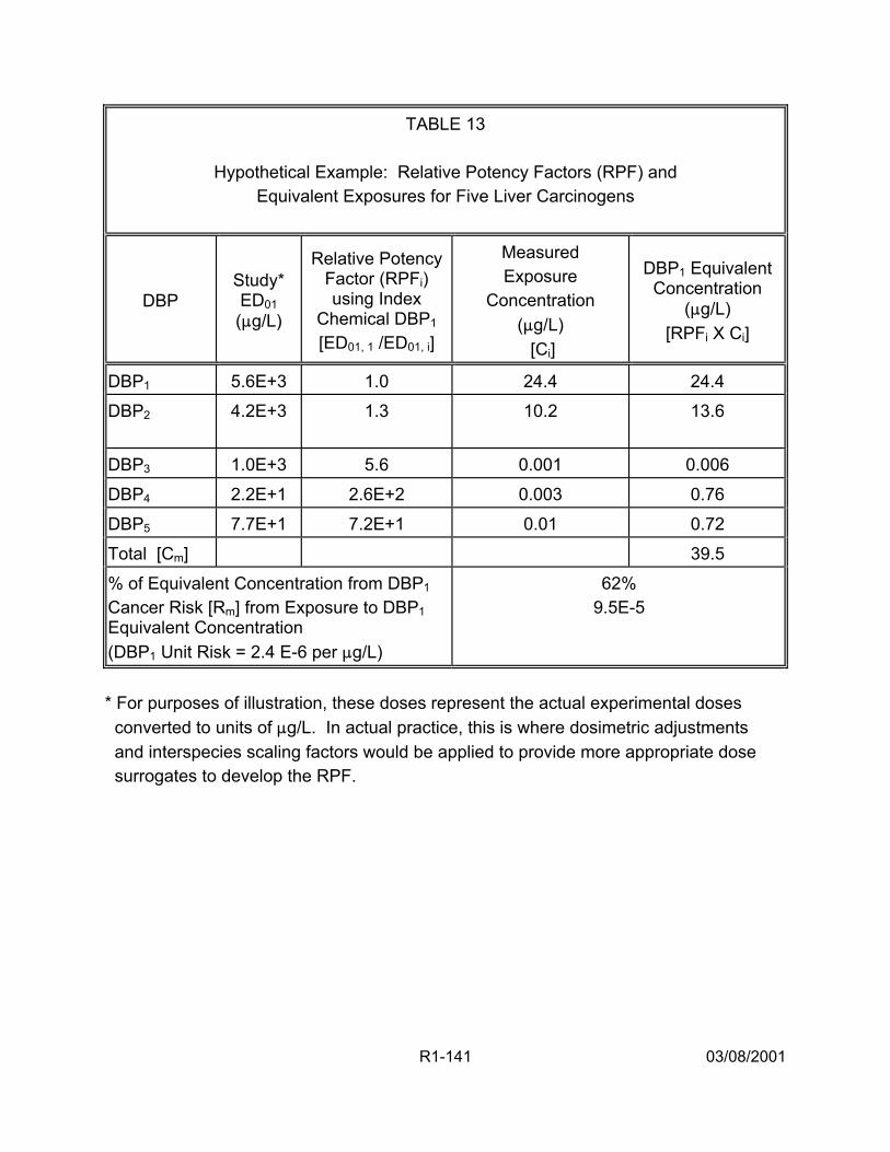
TABLE 13
Hypothetical Example: Relative Potency Factors (RPF) and Equivalent Exposures for Five Liver Carcinogens
DBP Study* ED01 (:g/L)
Relative Potency Factor (RPFi) using Index
Chemical DBP1 [ED01, 1 /ED01, i]
Measured Exposure
Concentration (:g/L) [Ci]
DBP1 Equivalent Concentration
(:g/L) [RPFi X Ci]
DBP1 5.6E+3 1.0 24.4 24.4 DBP2 4.2E+3
1.3
10.2
13.6
DBP3 1.0E+3 5.6 0.001 0.006 DBP4 2.2E+1 2.6E+2 0.003 0.76 DBP5 7.7E+1 7.2E+1 0.01 0.72 Total [Cm] 39.5 % of Equivalent Concentration from DBP1 Cancer Risk [Rm] from Exposure to DBP1 Equivalent Concentration (DBP1 Unit Risk = 2.4 E-6 per :g/L)
62% 9.5E-5
* For purposes of illustration, these doses represent the actual experimental doses converted to units of :g/L. In actual practice, this is where dosimetric adjustments and interspecies scaling factors would be applied to provide more appropriate dose surrogates to develop the RPF.
R1-141 03/08/2001
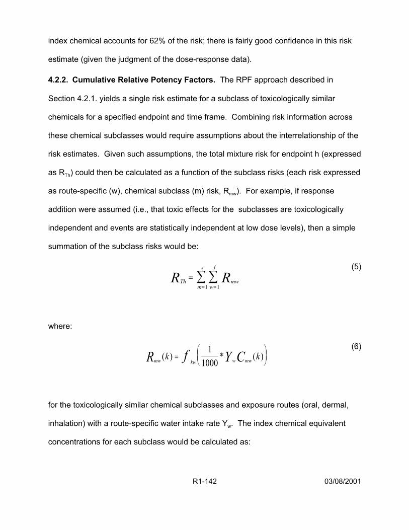
index chemical accounts for 62% of the risk; there is fairly good confidence in this risk
estimate (given the judgment of the dose-response data).
4.2.2. Cumulative Relative Potency Factors. The RPF approach described in
Section 4.2.1. yields a single risk estimate for a subclass of toxicologically similar
chemicals for a specified endpoint and time frame. Combining risk information across
these chemical subclasses would require assumptions about the interrelationship of the
risk estimates. Given such assumptions, the total mixture risk for endpoint h (expressed
as RTh) could then be calculated as a function of the subclass risks (each risk expressed
as route-specific (w), chemical subclass (m) risk, Rmw). For example, if response
addition were assumed (i.e., that toxic effects for the subclasses are toxicologically
independent and events are statistically independent at low dose levels), then a simple
summation of the subclass risks would be:
s j (5)RTh = ∑ ∑ Rmw
m=1 w=1
where:
1 (6) kRmw ( ) = f
kw 1000
*Y Cmw (k )
w
for the toxicologically similar chemical subclasses and exposure routes (oral, dermal,
w. The index chemical equivalent
concentrations for each subclass would be calculated as:
inhalation) with a route-specific water intake rate Y
R1-142 03/08/2001
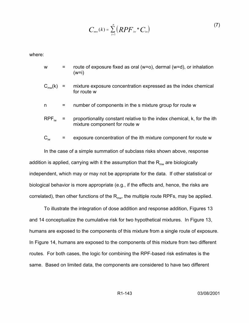
n
kCmw ( ) = ∑ ( RPFiw * Ciw) (7)
i=1
where:
w = route of exposure fixed as oral (w=o), dermal (w=d), or inhalation (w=i)
Cmw(k) = mixture exposure concentration expressed as the index chemical for route w
n = number of components in the s mixture group for route w
RPFiw = proportionality constant relative to the index chemical, k, for the ith mixture component for route w
Ciw = exposure concentration of the ith mixture component for route w
In the case of a simple summation of subclass risks shown above, response
addition is applied, carrying with it the assumption that the Rmw are biologically
independent, which may or may not be appropriate for the data. If other statistical or
biological behavior is more appropriate (e.g., if the effects and, hence, the risks are
correlated), then other functions of the Rmw, the multiple route RPFs, may be applied.
To illustrate the integration of dose addition and response addition, Figures 13
and 14 conceptualize the cumulative risk for two hypothetical mixtures. In Figure 13,
humans are exposed to the components of this mixture from a single route of exposure.
In Figure 14, humans are exposed to the components of this mixture from two different
routes. For both cases, the logic for combining the RPF-based risk estimates is the
same. Based on limited data, the components are considered to have two different
R1-143 03/08/2001
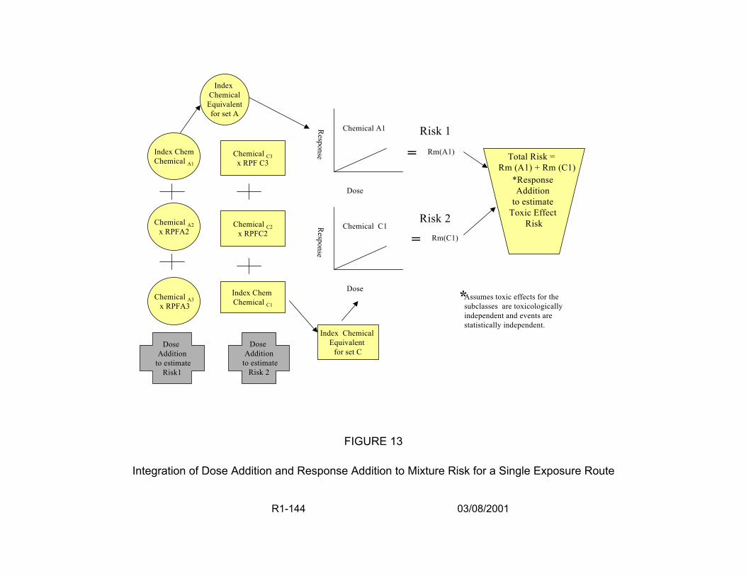
Index Chem Chemical A1
Chemical C3 x RPF C3
Index Chemical
Equivalent for set A
Chemical A1
Rm(A1)=
Dose
Chemical A2 x RPFA2
Risk 2Chemical C2 x RPFC2
Index Chem Chemical C1
Dose Addition
to estimate Risk 2
Index Chemical Equivalent
for set C
Dose
Response
Chemical C1 Rm(C1)=
*Response Addition
to estimate Toxic Effect
Risk
Total Risk = Rm (A1) + Rm (C1)
Chemical A3 x RPFA3
*Assumes toxic effects for the subclasses are toxicologically independent and events are statistically independent.
Dose Addition
to estimate Risk1
FIGURE 13
Integration of Dose Addition and Response Addition to Mixture Risk for a Single Exposure Route
R1-144 03/08/2001
Risk 1Response
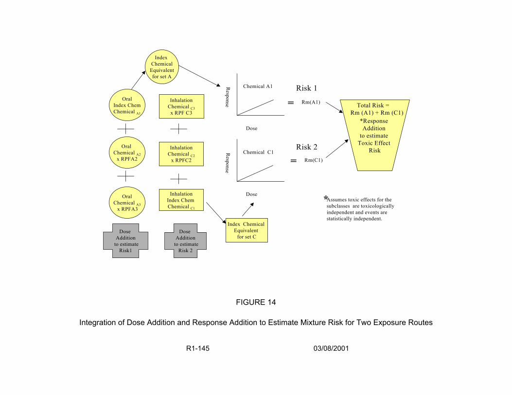
Oral Index Chem Chemical A1
Inhalation Chemical C3
x RPF C3
Index Chemical
Equivalent for set A
Chemical A1
Rm(A1)=
Dose
Risk 2 Rm(C1)=
Risk 1Respon
*Response Addition
to estimate Toxic Effect
Risk
Total Risk = Rm (A1) + Rm (C1)
se
Oral Chemical A2
x RPFA2
Oral Chemical A3
x RPFA3
Inhalation Chemical C2
x RPFC2
Inhalation Index Chem Chemical C1
Dose Addition
to estimate Risk 2
Index hemical Equivalent
for set C
Dose
Response
Chemical C1
C
*Assumes toxic effects for the subclasses are toxicologically independent and events are statistically independent.
Dose Addition
to estimate Risk1
FIGURE 14
Integration of Dose Addition and Response Addition to Estimate Mixture Risk for Two Exposure Routes
R1-145 03/08/2001
MOA. Because of this, the components are subdivided into two sets for development of
RPFs. Toxicity data (measured in % responding) is available for chemicals in both sets.
An index chemical is determined and index chemical equivalent exposure
concentrations are developed for each set. The toxicological evidence from the two
index chemicals indicates that the same target organ is affected. The low
environmental concentrations lead to exposure assessments in the low dose region. In
this exposure region, component interactions are assumed not to be significant. The
MOA data indicate there is toxicologic independence of action. Based on these data,
response addition is selected as an appropriate method to estimate the risk associated
with the two index chemical equivalent concentrations. Risks are estimated for each
index chemical using its dose-response curve at the index chemical equivalent
exposure concentration. The component risks from each RPF set are added.
Table 14 continues the illustration (see Tables 12 and 13) by presenting a
hypothetical characterization of three RPF risk estimates that have been made for the
same DBP mixture, but for different exposure routes (Figure 14) and different cancer
sites. Ways to combine these risks depend on what is known about the independence
of the toxicologic mechanism of action for the groups of chemicals and their route- and
chemical-specific effects. If these three effects are considered functionally independent,
then the mixture risk is based on a response addition assumption, Equation 5. The total
mixture risk of any cancer is their sum (e.g., Rm(k) = 9.5E-5 + 4.9E-5 + 2.2E-5 = 1.7E-4).
If the assumptions of toxicologic or statistical independence cannot be met, then other
functions of the risks could be used or the maximum of the three risks may serve as the
mixture risk estimate.
R1-146 03/08/2001

TABLE 14
Hypothetical Characterization of Several Relative Potency Factors For the Same DBP Mixture; Different Routes, Different Effects
Index Chemical
(DBP)
Equivalent Concentration /
Unit Risk
Attributable to Index
Chemical
Mixture Risk
Estimate
Route of Exposure
Toxicologic Effect of Concern
DBP1
39.5 (:g/L) 2.4 E-6 (:g/L)-1
62% 9.5E-5 Oral Liver Cancer
DBPq 27.3 (:g/L) 1.8E-6 (:g/L)-1
69% 4.9E-5 Oral Kidney Cancer
DBPr 1.7 (:g/m3) 1.3E-5 (:g/m3)-1
55% 2.2E-5 Inhalation Kidney Cancer
4.2.3. Unidentified DBPs. The initial response addition assessment shown in Section
2.6. estimated an additional amount of risk for the unidentified DBPs by determining a
fraction of the unidentified DBPs that can be associated with a given health endpoint and
assuming equal risk per concentration of organic halide material for both the measured
and the unidentified components of the mixture. A similar approach could be applied
during development of the RPF risk estimates, using information from either laboratory
data or from Quantitative Structure Toxicity Relationship models. The index chemical
equivalent concentration, Cm(k), could be adjusted to reflect the concentration of the
unidentified DBPs, Cu, that can be associated with the subclass being evaluated. A
relative potency factor, RPFu, for the unidentified DBPs in Cu could be estimated using
what is known about the likely chemical characterization of the unidentified DBPs (see
R1-147 03/08/2001
Section 2.5. and Appendix R1-A). For the same end point and route of exposure,
Equation 4 could then be adjusted by using Cu and RPFu to increase the value of Cm(k),
reflecting the contribution of the unidentified DBPs to that subclass of toxicologically
similar chemicals.
4.2.4. Discussion. The development of RPF-based risk estimates and their integration
with response addition in a CRPF approach addresses many of the shortcomings of the
first response addition assessment in Appendix I: Workshop Pre-meeting Report, but
not all issues are addressed. As shown above, the approach does not directly address
the differences in risks for sensitive subpopulations or the contribution to the risk
estimate that may be addressed by using what is known in the epidemiologic literature.
In addition, application of CRPF promises to be a resource-intensive exercise that may
be more technically correct than the application of response addition, but, in the end,
may not produce risk estimates very different in magnitude. Furthermore, an enormous
problem lies in the fact that very little toxicity data are available for the dermal and
inhalation routes of exposure.
The CRPF approach described here is a conceptual model for development of a
cumulative risk assessment for DBP mixtures. As shown, it improves on the initial
response addition assessment (Appendix I: Workshop Pre-meeting Report) by more
carefully considering toxicologic similarities among chemicals, routes of exposure, and
dosimetry. It allows for treatment system-specific exposures to be investigated and,
although not specified in this discussion, does not preclude the use of human activity
patterns and distribution system effects from incorporation into the analysis. A
R1-148 03/08/2001

probabilistic analysis and full risk characterization would be required with careful
treatment of the variabilities and uncertainties examined and explained.
R1-149 03/08/2001
5. RESEARCH NEEDS
DBP mixtures research is essential to establishing, explaining and estimating any
substantive human health risks from exposure to the low levels of DBPs found in
drinking water. Such research can serve to bridge the gap between the weak to
moderate associations with cancer and developmental effects suggested in the
epidemiologic literature and effects found only at high-dose levels of DBPs in single-
chemical animal bioassays. To strengthen the risk assessment, a multidisciplinary
research approach is needed that includes investigations of statistical methods and
quantitative analyses, risk assessment methodologies, toxicologic effects, epidemiologic
cohorts, and exposure assessment. Section 3 presented approaches that have the
potential to be applied in the near term. The research ideas presented here represent
long-term needs that are also considered important to improving the DBP mixture risk
assessment.
5.1. METHODS RESEARCH
• Develop more scientifically credible distributions of toxicity coefficients for all endpoints (e.g., slope factors, effective dose levels) for use in probabilistic assessments.
• Investigate dose-response models for developmental and reproductive effects that include parameters for threshold and litter effects and incorporate multiple endpoints.
• Develop comprehensive exposure models that incorporate multiple routes, human activity patterns, multiple chemicals, and endpoint-specific timing of exposures.
R1-150 03/08/2001
• Apply alternative methods to Monte Carlo analysis (e.g., bootstrapping, Latin Hypercube, analytic solutions) to addressing uncertainty analysis and sensitivity analysis.
5.2. RESEARCH ON APPLICATION OF A CUMULATIVE RELATIVE POTENCY FACTOR APPROACH
• Define subclasses of DBPs based on exposure route, chemical structure, physicochemical attributes of chemicals, and MOA considerations (components may be in more than one subclass depending on route of exposure).
• Determine relationships among subclasses from a toxicologic perspective, including MOA, PK, PD, and consideration of what level of organization the effect measure was observed. Use relationships to develop appropriate assumptions and methods for combining RPF-based risks.
• Refine and apply dosimetric adjustment methods using case studies. Parallel suites of model structures are needed across all three routes (oral, inhalation, and dermal) based on inhalation reference concentration methods as a platform for consistency (U.S. EPA, 1994a). New model structures can be extended to include key determinants of MOA: dose surrogates to incorporate PK and PD parameters and processes at both portal-of-entry and systemic sites of toxicity. These dose surrogates can be constructed to be commensurate with the level of observation of the effect measure (population or cellular).
• Refine exposure assessments to consider water use issues (bathing, cooking, dishwashing), effects of heating water on chemical composition, human activity patterns and the human condition at time of exposure (age, weight, health status).
5.3. EPIDEMIOLOGIC RESEARCH
• Continue to rule out non-causal explanations for epidemiologic findings by examining reasonable alternative hypotheses for positive study results. To decrease the uncertainties associated with the interpretation
R1-151 03/08/2001
of this body of literature, it is necessary to develop better assessment methods for the DBPs and other exposures of interest.
• Expand ongoing or planned epidemiologic studies to include measures of dermal and inhalation exposures and human activity patterns for use in cumulative risk assessments.
• Quantitatively identify the model and data uncertainties in the exposure-response analysis used in the epidemiologic literature.
• Define susceptibility responses for general population and sensitive subpopulations.
• Develop and use biomarkers of exposure in future analytical epidemiologic studies because this can help reduce exposure misclassification. Instead of classifying epidemiologic study participants in a broad exposure category (e.g., as being exposed to disinfected water or to water without disinfection), measure and identify specific DBPs and consider the water usage, consumption rates and human activity patterns to better estimate exposure.
• Promote understanding of the problems associated with using a single aggregate number from a meta-analysis of the epidemiologic data for quantitative risk assessment, including considerations of whether causality can be established; take into consideration possible publication bias (i.e., when studies that fail to find an association, or find responses in different sites, are not published and not available for meta-analysis)
5.4. DEVELOPMENT OF TOXICOLOGIC DATA
• Conduct toxicologic studies to determine effects caused by inhalation and dermal DBP exposure and enrich the database for cumulative risk assessment.
• Use physiology-based pharmacokinetic models for the different DBPs, combined with available information on mode of action to provide insight into patterns of tumor development in animals and humans. In addition, use both in vivo and in vitro studies to help identify components of chlorinated water that may be associated with effects seen in the
R1-152 03/08/2001

positive epidemiologic studies (e.g., bladder cancer, spontaneous abortion).
• Study gene-environment interactions (e.g., CYP2E1, GST, acetyl) to identify subpopulations for further epidemiologic study; epidemiologic studies focusing on colon polyps could provide important information.
• Generate DBP mixtures data useful to refine human health risk assessment methods under development and efficient experimental designs and statistical approaches for mixtures. Mixtures of THM and HAA have a limited database already. Future directions include the evaluation of more cross-class mixtures of the THM and HAA, eventually adding other DBPs of concern, such as bromate, and screening for combinations of DBPs that may exhibit additivity or interaction effects.
• Conduct carefully designed experiments to estimate the toxicity of complex mixtures of DBPs produced by using reproducible disinfection scenarios or extracts of finished drinking water. Using these data in conjunction with the data on defined mixtures, estimates can then be made of the potential toxicity of unidentified DBP material in finished drinking water.
• Conduct studies to determine the mode(s)-of-action of DBPs, the mechanism(s) underlying any identified nonadditive interactions and their relevance to humans for cancer, developmental, and reproductive effects. Mode-of-action is difficult to determine, but is critical not only to understanding toxicity, but also to the development of statistical risk models based on biologic assumptions (e.g., independence of action, similar toxicologic action).
• Link exposure to biokinetic models so differences in toxicokinetics can aid in interpreting time, route, and cross species extrapolations. Include considerations of dosimetry and level of organization of the toxic response (e.g., cellular vs. population-based) in the risk assessment.
• Apply appropriately genetically altered (transgenic) animal models when the mechanism of action has been determined at the genetic level to determine the quantitative contribution of that mechanism to the chemical’s overall toxicity.
R1-153 03/08/2001
• Develop appropriate laboratory test systems as a screen for the myriad of DBPs that have been identified in finished drinking water. Investigations into short-term screening tests for DBP mixtures, such as in vivo systems (e.g., developmental effects/cancer in medaka; mutagenicity in the frog embryo (FETAX) assay) or in vitro procedures (e.g., carcinogenicity in Syrian hamster embryo (SHE) cell transformation assay; developmental effects in whole embryo culture systems) are needed to identify the potential toxicity of DBP mixtures. The most toxic mixtures can then be tested in appropriate rodent test systems for reproductive, developmental, hepatotoxic, nephrotoxic, carcinogenic or immunotoxic effects.
R1-154 03/08/2001
6. REFERENCES
Allen, B., K. Crump and A. Shipp. 1988. Correlation between carcinogenic potency of chemicals in animals and humans. Risk Anal. 8: 531-544.
Allen, B., K. Crump and A. Shipp. 1998. Is it possible to predict the carcinogenic potency of a chemical in humans using animal data? Banbury Report 31: Carcinogen Risk Assessment: New Directions in the Qualitative and Quantitative Aspects. Cold Spring Harbor Laboratory, New York. p. 197-209.
Aschengrau, A., S. Zierler and A. Cohen. 1993. Quality of community drinking water and the occurrence of late adverse pregnancy outcomes. Arch. Environ. Health. 48(2): 105-114.
Bove, F.J., M.C. Fulcomer, J.B. Klotz, J. Esmart, E.M. Dufficy and J.E. Savrin. 1995. Public drinking water contamination and birth outcomes. Am. J. Epidemiol. 141(9): 850-862.
Bull, R.J. and F.C. Kopfler. 1991. Health effects of disinfectants and disinfection byproducts. AWWA Research Foundation.
Bunge, A. and J. McDougal. 1999. Chapter 6, Dermal Uptake. In: Exposure to Contaminants in Drinking Water: Estimating Uptake through the Skin and by Inhalation, S. Olin, Ed. CRC Press, Washington, DC. p. 137-181.
Canada Ministry of Health and Welfare. 1981. Tapwater consumption in Canada. Document No. 82-EHD-80. Public Affairs Directorate, Department of National Health and Welfare, Ottawa Canada.
Cantor, K.P., R. Hoover, P. Hartge et al. 1987. Bladder cancer, drinking water source, and tap water consumption: A case-control study. J. Natl. Cancer Inst. 79: 1269-1279.
Cantor, K.P., C.F. Lunch, M. Hildesheim et al. 1998. Drinking water source and chlorination byproducts. I. Risk of bladder cancer. Epidemiology. 9: 21-28.
Cassee, F.R., J.P. Groten, P.J. Van Bladeren and V.J. Feron. 1998. Toxicological evaluation and risk assessment of chemical mixtures. Crit. Rev. Toxicol. 28: 73-101.
R1-155 03/08/2001

Chen, J.J. D.W. Gaylor and R.L. Kodell. 1990. Estimation of the joint risk from multiple-compound exposure based on single-compound experiments. Risk Anal. 10(2): 285-290.
Christ, S.A., E.J. Read, J.A. Stober and M.K. Smith. 1995. The developmental toxicity of bromochloroacetonitrile in pregnant Long-Evans rats. Internat. J. Environ. Health Res. 5: 175-188.
Clark, R.M. 1998. Chlorine demand and TTHM formation kinetics: A second order model. J. Environ. Eng. 124(1): 16-24.
Clark, R.M. and M. Sivaganesan. 1998. Predicting chlorine residuals and the formation of TTHMs in drinking water. J. Environ. Eng. 124(12): 1203-1210.
Cogliano, V.J. 1997. Plausible upper bounds: Are their sums plausible? Risk Anal. 17(1): 77-84.
Cogliano, V.J. 1998. Assessing the cancer risk from environmental PCBs. Environ. Health Perspect. 106(6): 317-323.
Corley, R.A., S.M. Gordon and L.A. Wallace. 2000. Physiologically based pharmacokinetic modeling of the temperature-dependent dermal absorption of chloroform in humans following bath water exposures. Toxicol. Sci. 53:3-23.
Cragle, D.L., C.M. Shy, R.J. Struba and E.J. Stiff. 1985. A case-control study of colon cancer and water chlorination in North Carolina. In: Water Chlorination: Chemistry, Environmental Impact, and Health Effects, R.L. Jolley, R.J. Bull, W.P. Davis et al., ed. Lewis Publishers, Inc., Chelsea, MI. Vol. 5, p. 153-159.
Craun, G.F. et al. 1993. Conference conclusions—Safety of water disinfection: Balancing chemical and microbial risks, G.F. Craun, Ed. ILSI Press, Inc., Washington, DC. p. 657-667.
Crosby, L.M., K.T. Morgan, B. Gaskill, D.C. Wolff and A.B. DeAngelo. 2000. Origin and distribution of potassium bromate-induced testicular and peritoneal mesothelioma in rats. Toxicol. Pathol. 28: 253-266.
Crouch, E.A.C. 1996. Uncertainty distributions for cancer potency factors: Laboratory animal carcinogenicity bioassays and interspecies extrapolation. Human Ecolog. Risk Assess. 2(1): 103-129.
R1-156 03/08/2001
da Silva, M.L., G. Charest-Tardif, K. Krishnan and R. Tardif. 1999a. Influence of oral administration of a quaternary mixture of trihalomethanes on their blood kinetics in the rat. Toxicol. Lett. 106: 49-57.
da Silva, M.L., G. Charest-Tardif, K. Krishnan and R. Tardif. 1999b. Pharmacokinetic interactions between orally-administered trihalomethanes in the rat. Abstract 28, Second International Conference on the Safety of Water Disinfection: Balancing Chemical and Microbial Risks.
Davis, M.E. 1992. Dichloroacetic acid and trichloroacetic acid increase chloroform toxicity. J. Toxicol. Environ. Health. 37: 139-148.
DeAngelo, A.B., M.H. George, S.R. Kilburn, T.M. Moore and D.C. Wolff. 1998. Carcinogenicity of potassium bromate administered in the drinking water to male B6C3F1 mice and F344/N rats. Toxicol. Pathol. 26: 587-594.
DeMarini, D.M., A. Abu-Shakra, C.F. Felton, K.S. Patterson and M.L. Shelton. 1995. Mutation spectra in Salmonella of chlorinated, chloraminated or ozonated drinking water extracts: Comparison to MX. Environ. Molecul. Mutagen. 26: 270-285.
DeMarini, D.M., M.L. Shelton, S.H. Warren et al. 1997. Glutathione S-transferasemediated induction of GC÷AT transitions by halomethanes in Salmonella. Environ. Molecul. Mutagen. 30: 440-447.
Dodds, L., W. King, C. Woolcott and J. Pole. 1999. Trihalomethanes in public water supplies and adverse birth outcomes. Epidemiology. 10(3): 233-237.
Doyle, T.J., W. Zheng, J.R. Cerhan et al. 1997. The association of drinking water source and chlorination by-products with cancer incidence among post-menopausal women in Iowa: A prospective cohort study. Am. J. Publ. Health. 87: 1168-1176.
Ershow, A.G. and K.P. Cantor. 1989. Total water and tapwater intake in the United States; population-based estimates of quantities and sources. Life Sciences Research Office, Federation of American Societies for Experimental Biology.
Ershow, A.G., L.M. Brown and K.P. Cantor. 1991. Intake of tapwater and total water by pregnant and lactating women. Am. J. Publ. Health. 81: 328-334.
Evans, J.S., G.M. Gray, R.L Sielken, Jr., A.E. Smith, C. Valdez-Flores and J. Graham. 1994. Use of probabilistic expert judgment in uncertainty analysis of carcinogenic potency. Reg. Toxicol. Pharmacol. 20: 15-36.
R1-157 03/08/2001
Fair, P.S. 1995. Influence of water quality on formation of chlorination by-products. In: Disinfection By-products in Drinking Water: Critical Issues in Health Effects Research: Workshop Report. ILSI Press. p. 14-17.
Fayerweather, W.E., J.J. Collins, A.R. Schnatter, F.T. Hearne, R.A. Menning and D.P. Reyner. 1999. Quantifying uncertainty in a risk assessment using human data. Risk Anal. 19(6): 1077-1090.
Freedman, M., K.P. Cantor, N.L. Lee et al. 1997. Bladder cancer and drinking water: A population-based case-control study in Washington County, Maryland (United States). Cancer Causes and Control. 8: 738-744.
Gallagher, M.D., J.R. Nuckols, L. Stallones and D.A. Savitz. 1998. Exposure to trihalomethanes and adverse pregnancy outcomes. Epidemiology. 9(5): 484-489.
Gennings, C., P. Schwartz, W.H. Carter, Jr. and J.E. Simmons. 1997. Detection of departures from additivity in mixtures of many chemicals with a threshold model. J. Agric. Biol. Environ. Stat. 2: 198-211.
Gennings, C., L. Teuschler, W.R. Hartley, A. Thiyagarajah and J.E. Simmons. 1999. Novel Statistical Methods for Risk Assessment of Water Disinfection By-products. Proceedings of the AWWA Conference TU 22.2 (CD ROM).
George, M.H., T. Moore, S. Kilburn, G.R. Olson and A.B. DeAngelo. 2000. Carcinogenicity of chloral hydrate administered in drinking water to the male F344/N rat and male B6C3F1 mouse. Toxicol. Pathol. 28(4): 610-618.
Gessner, P.K. 1988. A straightforward method for the study of drug interactions: An isobolographic primer. J. Am. College Toxicol. 7: 987-1012.
Giardino, N. and J. Andelman. 1996. Characterization of the emissions of trichloroethylene, chloroform, and 1,2-dibromo-3-chloropropane in a full-size, experimental shower. J. Expos. Anal. Env. Epi. 6(4): 413-423.
Gonzalez-Leon, A., J.L. Merdink, R.J. Bull and I.R. Schultz. 1999. Effect of pretreatment with dichloroacetic or trichloroacetic acid in drinking water on the pharmacokinetics of a subsequent challenge dose in B6C3F1 mice. Chem. Biol. Interact. 123(3): 239-253.
R1-158 03/08/2001
Hartley, W.R., C. Gennings, L. Teuschler, A. Thiyagarajah and J.E. Simmons. 1999. Advances in the Toxicological Assessment of Disinfection By-products in Rodent and Fish Biomedical Models. Proceedings of the AWWA Conference TU 22.1 (CD ROM).
Hattis, D. and K. Barlow. 1996. Human interindividual variability in cancer risks — Technical and management challenges. Human Ecolog. Risk Assess. 2: 194-220.
Hattis, D. and R. Goble. 1991. Expected values for projected cancer risks from putative genetically-acting agents. Risk Anal. 11: 359-363.
Hattis, D. and W.S. Minkowitz. 1996. Risk evaluation: Criteria arising from legal traditions and experience with quantitative risk assessment in the United States. Environ. Toxicol. Pharmacol. 2: 103-109.
Hertzberg, R.C., G. Rice and L.K. Teuschler. 1999. Methods for health risk assessment of combustion mixtures. In: Hazardous Waste Incineration: Evaluating the Human Health and Environmental Risks, S. Roberts, C. Teaf, J. Bean, Ed. CRC Press. p.105-148.
Hildesheim, M.E., K.P. Cantor, C.F. Lynch et al. 1998. Drinking water source and chlorination by-products. II. Risk of colon and rectal cancers. Epidemiology. 9: 29-35.
IARC (International Agency for Research on Cancer). 1991. Chlorinated drinking-water; chlorination by-products; some other halogenated compounds; cobalt and cobalt compounds, In: Monographs on the evaluation of carcinogenic risks to humans, vol. 52. World Health Organization, Lyon, France.
ILSI (International Life Sciences Institute). 1998. The Toxicity and Risk Assessment of Complex Mixtures in Drinking Water. Report prepared for the U.S. EPA’s Office of Water. March.
ILSI (International Life Sciences Institute). 1999. A Framework for Cumulative Risk Assessment. Workshop Report, B. Mileson, E. Faustman, S. Olin, P. Ryan, S. Ferenc and T. Burke, ed. ILSI Press, Washington, DC.
Jo, W.K., C.P. Weisel and P.J. Lioy. 1990. Chloroform exposure and body burden from showering with chlorinated tap water. Risk Anal. 10: 575-580.
R1-159 03/08/2001
Johnson, T., P. Hakkinen and D. Reckhow. 1999. Chapter 3, Exposure Characteristics. In: Exposure to Contaminants in Drinking Water: Estimating Uptake through the Skin and by Inhalation, S. Olin, ed. CRC Press, Washington, DC. p. 31-84.
Kanitz, S., Y. Franco, Y. Patrone, V. Caltabellotta et al. 1996. Association between drinking water disinfection and somatic parameters at birth. Environ. Health Perspect. 104(5): 516-520.
Keegan, T.E., R.A. Pegram and J.E. Simmons. 1997. Assessment of the hepatotoxic interaction between chloroform and bromodichloromethane by dose addition and response. The Toxicol. 17: 780.
King, W.D. and L.D. Marrett. 1996. Case-control study of water source and bladder cancer. Cancer Causes and Control. 7: 596-604.
Klinefelter, G.R., J.D. Suarez, N.L. Roberts and A.B. DeAngelo. 1995. Preliminary screening for the potential of drinking water disinfection byproducts to alter male reproduction. Repro. Toxicol. 9(6): 571-578.
Klotz, J.B. and L.A. Pyrch. 1999. Neural tube defects and drinking water disinfection by-products. Epidemiology. 10(4): 383-390.
Kodell, R.L., A.P. Basu and D.W. Gaylor. 1996. On interspecies correlations of carcinogenic potencies. J. Toxicol. Environ. Health. 48(3): 231-237.
Kramer, M.D., C.F. Lynch, P. Isacson and J.W. Hanson. 1992. The association of waterborne chloroform with intrauterine growth retardation. Epidemiology. 3(5): 407-413.
Krasner, S.W., M.J. McGuire, J.G. Jacangelo, N.L. Patania, K.M. Reagan and E.M. Aieta. 1989. The occurrence of disinfection byproducts in U.S. drinking water. JAWWA. 81: 41-53.
Krishnan, K. and J. Brodeur. 1991. Toxicological consequences of combined exposures to environmental pollutants. Arch Complex Environ. Studies. 3(3):1-106.
Kurata, Y., B.A. Diwan and J.M. Ward. 1992. Lack of renal tumour-initiating activity of a single dose of potassium bromate, a genotoxic renal carcinogen in male F344/NCr rats. Food. Chem. Toxicol. 30(3): 251-259.
R1-160 03/08/2001
Kurokawa, Y., S. Aoki, Y. Matsushima, N. Takamura, T. Imazawa and Y. Hayashi. 1986. Dose-response studies on the carcinogenicity of potassium bromate in F344 rats after long-term oral administration. J. Natl. Cancer Inst. 77(4): 977-982.
Kurokawa, Y., Y. Hayashi, A. Maekawa, M. Takahashi, T. Kokubo and S. Odashima. 1983. Carcinogenicity of potassium bromate administered orally to F344 rats. J. Nat. Cancer Inst. 71(5): 965-972.
Lang, J.M., K.J. Rothman and C.L. Cann. 1998. That confounded p-value (editorial). Epidemiology. 9(1): 7-8.
Lewtas, J. 1985. Development of a comparative potency method for cancer risk assessment of complex mixtures using short-term in vivo and in vitro bioassays. Toxicol. Ind. Health. 1: 193-203.
Lewtas, J. 1988. Genotoxicity of complex mixtures: Strategies for the identification and comparative assessment of airborne mutagens and carcinogens from combustion sources. Fund. Appl. Toxicol. 10: 571-589.
Linder, R.E., G.R. Klinefelter, L.F. Strader, J.D. Suarez, N.L. Roberts and C.J. Dyer. 1994. Spermatotoxicity of dibromoacetic acid in rats after 14 daily exposures. Repro. Toxicol. 8: 251-259.
Magnus, P., J.J.K. Jaakkola, A. Skrondal et al. 1999. Water chlorination and birth defects. Epidemiology. 10(5): 513-517.
McGeehin, M.A. et al. 1993. Case-control study of bladder cancer and water disinfection methods in Colorado. Am. J. Epidemiol. 138: 492-501.
McKone, T. 1987. Human exposure to volatile organic compounds in household tap water in the indoor inhalation pathway. Environ. Sci. Technol. 21: 1194-1201.
Mills, C.J., R.J. Bull, K.P. Cantor et al. 1998. Workshop report. Health risks of drinking water chlorination by-products: Report of an expert working group. Chronic Dis. Canada. 19(3): 1-16.
Miltner, R.J., E.W. Rice and A.A. Stevens. 1990. Pilot-scale investigation of the formation and control of disinfection by-products. In: 1990 Annual Conference Proceedings. AWWA Annual Conference, Cincinnati, OH. 2:1787-1802.
R1-161 03/08/2001
Moudgal, C.J., J.C. Lipscomb and R.M. Bruce. 2000. Potential health effects of drinking water disinfection by-products using quantitative structure activity relationships. Toxicol. 147: 109-131.
Mumtaz, M.M. and P.R. Durkin. 1992. A weight-of-evidence scheme for assessing interactions in chemical mixtures. Toxicol. Indus. Health. 8: 377-406.
Mumtaz, M.M., C.T. de Rosa, J. Groten et al. 1997a. Evaluation of chemical mixtures of public health concern: Estimation vs. experimental determination of toxicity. Environ. Health Perspect. 106: 1353-1360.
Mumtaz, M.M., J.A. Parer and J.T. Coleman. 1997b. Risk assessment for chemical mixtures: Fine-tuning the hazard index approach. J. Clean Technol. Environ. Toxicol. Occup. Med. 6(2): 189-204.
Mumtaz, M.M., C.T. DeRosa, J. Groten et al. 1998. Estimation of toxicity of chemical mixtures through modeling of chemical interactions. Environ. Health Perspect. 106(6): 1353-1360.
Murphy P.A., C. Poole, T. Harvey and S. Greenland. 1999. Meta-analysis of epidemiologic studies of chlorinated drinking water and cancer: contraindications to summary aggregation. Am. J. Epidemiol. 149: S5.
Murphy P.A., G.F. Craun, G. Amy, S. Krasner and S. Dundorf. 2000. Enhanced evaluation of disinfectant by-product exposures for the re-analysis of cancer risks in previously conducted epidemiological studies. Epidemiology. 11(4): S129.
Nesnow, S. 1990. Mouse skin tumours and human lung cancer: Relationships with complex environmental emissions. In: Complex Mixtures and Cancer Risk. IARC Scientific Publ. 104: 44-54.
Neutra, R.R. and B. Ostro. 1992. An evaluation of the role of epidemiology in assessing current and future disinfection technologies for drinking water. Sci. Total Environ. 127: 91-138.
NRC (National Research Council). 1983. Risk Assessment in the Federal Government: Managing the Process. Committee on the Institutional Means for Assessment of Risks to Public Health, Commission on Life Sciences. National Academy Press, Washington, DC.
R1-162 03/08/2001
NRC (National Research Council). 1988. Complex Mixtures: Methods for in Vivo Toxicity Testing, National Academy Press.
NTP (National Toxicology Program). 1992. Dibromoacetonitrile: Short-term reproductive and developmental toxicity study when administered to Sprague-Dawley rats in the drinking water. NTIS PB97-143127.
Olin, S., Ed. 1999. Exposure to Contaminants in Drinking Water: Estimating Uptake through the Skin and by Inhalation. International Life Sciences Institute. CRC Press, Washington, DC.
Patterson, K.S., B.W. Lydins, Jr. and S.D. Richardson. 1995. Mutagenicity of drinking water following disinfection. Aqua. 44: 1-9.
Paustenbauch, D. 2000. The practice of exposure assessment: A state of the art review. J. Toxicol. Environ. Health. Part B. 3: 179-291.
Pereira, M.A. 1994. Route of administration determines whether chloroform enhances or inhibits cell proliferation in the liver of B6C3F1 mice. Fund. Appl. Toxicol. 23(1): 87-92.
Pereia, M.A. and L.W. Chang. 1982. Binding of chloroform to mouse and rat hemoglobin. Chem. Biol. Interact. 39(1): 89-99.
Pereira, M.A. and P.M. Kramer. 1999. Effect of chloroform in combination with dichloroacetic acid or trichloroacetic acid on N-methylnitrosourea-initiated liver and kidney tumors in B6C3F1 mice (abstract 50). Second International Conference on the Safety of Water Disinfection: Balancing Chemical and Microbial Risks.
Pereira, M.A., K. Li and P.M. Kramer. 1997. Promotion by mixtures of dichloroacetic acid and trichloroacetic acid of N-methyl-N-nitrosourea-initiated cancer in the liver of female B6C3F1 mice. Cancer Lett. 115: 15-23.
Poole, C. 1997. Analytical meta-analysis of epidemiologic studies of chlorinated drinking water and cancer: Quantitative review and reanalysis of the work published by Morris et al. Am. J. Publ. Health. 82: 955-963. A report to the National Center for Environmental Assessment, U.S. EPA, September 30, 1997.
Poole, C. and S. Greenland. 1999. Random-effects meta-analyses are not always conservative. Am. J. Epidemiol. 150: 469-475.
R1-163 03/08/2001
Randall, J.L., S.A. Christ, P. Horton-Perez, G.A. Nolen, E.J. Read and M.K. Smith. 1991. Developmental effects of 2-bromoacetic acid in the Long Evans rat. Teratol. 43: 454.
Regli, R., P. Beger, B. Macler and C. Haas. 1993. Proposed decision tree for management of risks in drinking water: Consideration for health and socioeconomic factors. In: Safety of Water Disinfection: Balancing Chemical and Microbial Risks, G.F. Craun, Ed. ILSI Press, Washington, DC. p. 39-80.
Reif, J.S., M.C. Hatch, M. Bracken, L.B. Holmes, B.A. Schwetz and P.C. Singer. 1996. Reproductive and developmental effects of disinfection by-products in drinking water. Environ. Health Perspect. 104(10): 1056-1061.
Rhomberg, L. 1999. Report of the Toxicology Breakout Group (BOG). Appendix B: A conceptual, graphical scheme for thinking about cumulative risk and exposure-time profiles. In: A Framework for Cumulative Risk Assessment, B. Mileson, E. Faustman, S. Olin, P.B. Ryan, S. Ferenc and T. Burke, Ed. ILSI (International Life Sciences Institute) Risk Science Institute Workshop Report. p. 21-23.
Rice, G., L.K. Teuschler, J. Cohen et al. 2001. Risk Assessment of Complex Mixtures of Disinfection Byproducts (DBPs): Methods for Considering Unidentified DBPs. In: Microbial Pathogens and Disinfection Byproducts in Drinking Water: Health Effects and Management of Risks. G.F. Craun, F.S. Hauchman, D.E. Robinson, ed., ILSI Press.
Richardson, S.D. 1998. Identification of drinking water disinfection by-products. In: John Wiley’s Encyclopedia of Environmental Analysis & Remediation, R.A. Meyers, ed. Vol. 3, p. 1398-1421.
Savitz, D.A., K.W. Andrews and L.M. Pastore. 1995. Drinking water and pregnancy outcome in central North Carolina: Source, amount, and trihalomethane levels. Environ. Health Perspect. 103(3): 592-596.
Schulte, P.A. 1989. A conceptual framework for the validation and use of biologic markers. Environ. Res. 48: 129-144.
Shipp, A., K. Crump and B. Allen. 1989. Correlation between carcinogenic potency of chemicals in animals and humans. Comments in Toxicol. 5/6: 289-303.
Sielken, R.L., Jr. 1995. How to use both human and animal data in quantitative risk assessment. In: The Role of Epidemiology in Regulatory Risk Assessment, John Graham, ed. Elsevier Science. p. 105-123.
R1-164 03/08/2001
Simmons J.E. 1994. Nephrotoxicity resulting from multiple chemical exposures and chemical interactions. In: Toxicology of Chemical Mixtures: Case Studies, Mechanisms and Novel Approaches, R.S.H. Yang, Ed. Academic Press, San Diego, CA. p. 335-360.
Simmons, J.E. 1995a. Special Issue: Chemical mixtures and quantitative risk assessment. Proceedings of a symposium sponsored by the Health Effects Research Laboratory of the U.S. EPA, Nov. 7-10, 1994. Toxicol. 105: (2)(3).
Simmons, J.E. 1995b. Chemical mixtures: Challenge for toxicology and risk assessment. Toxicol. 105: 111-120.
Simmons, J.E. and R.A. Pegram. 1998. NOAEL and LOAEL determinations of acute hepatotoxicity for chloroform and bromodichloromethane delivered in an aqueous vehicle to F344 rats. J. Toxicol. Environ. Health. Part A. 55: 65-75.
Simmons, J.E., C. Gennings, L.K. Teuschler and Y.M. Sey. 2000a. Evidence for dose additivity of chloroform and bromodichloromethane in mice. The Toxicologist. (In press)
Simmons, J.E., L.K. Teuschler and C. Gennings. 2000b. The toxicology of DBP mixtures: Methods for multi-chemical assessment, present research efforts, and future research directions. In: ILSI’s Second International Conference on the Safety of Water Disinfection: Balancing Chemical and Microbial Risks, G. Craun, Ed. (In Press)
Singer, P.C. 1995. Disinfection by-products: From source to tap. In: Disinfection By-products in Drinking Water: Critical Issues in Health Effects Research: Workshop Report. ILSI Press. p. 7-8.
Smith, M.K., J.L. Randall, D.R. Tocco, R.G. York, J.A. Stober and E.J. Read. 1988. Teratogenic effects of trichloroacetonitrile in the Long-Evans rat. Teratology. 38: 113-120.
Smith, M.K., J.L. Randall, J.A. Stober and E.J. Read. 1989a. Developmental toxicity of dichloroacetonitrile: A by-product of drinking water disinfection. Fund. Appl. Toxicol. 12: 765-772.
Smith, M.K., J.L. Randall, E.J. Read and J.A. Stober. 1989b. Teratogenic activity of trichloroacetic acid in the rat. Teratology. 40: 445-451.
R1-165 03/08/2001
Smith, M.K, J.L. Randall, E.J. Read and J.A. Stober. 1990. Developmental effects of chloroacetic acid in the Long-Evans rat. Teratology. 41: 593.
Smith, M.K., J.L. Randall, E.J. Read and J.A. Stober. 1992. Developmental toxicity of dichloroacetate in the rat. Teratology. 46: 217-223.
Stiteler, W.M., L.A. Knauf, R.C. Hertzberg and R.S. Schoeny. 1993. A statistical test of compatibility of data sets to a common dose response model. Reg. Toxicol. Pharmacol. 18: 392-402.
Svendsgaard, D.J. and R.C. Hertzberg. 1994. Statistical methods for the toxicological evaluation of the additivity assumption as used in the EPA chemical mixture risk assessment guidelines. In: Toxicology of Chemical Mixtures: Case Studies, Mechanisms, and Novel Approaches, R.S.H. Yang, Ed. Academic Press, NY. p. 599-642.
Takamura, N., Y. Kurokawa, Y. Matsushima, T. Imazawa, H. Onodera and Y. Hayashi. 1985. Long-term oral administration of potassium bromate in male Syrian golden hamsters. Sci. Rep. Res. Inst. Tohoku. Univ. Med. 32(1-4): 43-46.
Teuschler, L.K. and R.C. Hertzberg. 1995. Current and future risk assessment guidelines, policy, and methods development for chemical mixtures. Toxicology. 105: 137-144.
Teuschler, L.K., C. Gennings, W.M. Stiteler et al. 2000. A multiple-purpose design approach to the evaluation of risks from complex mixtures of disinfection by-products (DBPs). Drug Chem. Toxicol. 23(1): 307-321.
Umemura, T., K. Sai, A. Takagi, R. Hasegawa and Y. Kurokawa. 1993. A possible role for cell proliferation in potassium bromate (KBrO3) carcinogenesis. J. Cancer Res. Clin. Oncol. 119(8): 463-469.
Umemura, T., K. Sai, A. Takagi, R. Hasegawa and Y. Kurokawa. 1995. A possible role for oxidative stress in potassium bromate (KBrO3) carcinogenesis. Carcinogenesis. 16(3): 593-597.
U.S. EPA. 1986. Guidelines for the Health Risk Assessment of Chemical Mixtures. Federal Register. 51(185): 34014-34025.
U.S. EPA. 1989a. Risk Assessment Guidance for Superfund. Vol. 1. Human Health Evaluation Manual (Part A). EPA/540/1-89/002.
R1-166 03/08/2001
U.S. EPA. 1989b. Interim Procedures for Estimating Risks Associated with Exposures to Mixtures of Chlorinated Dibenzo-p-dioxins and -dibenzofurans (CDDs and CDFs) and 1989 update. Risk Assessment Forum. EPA/625/3-89/016. March.
U.S. EPA. 1990. Technical Support Document on Health Risk Assessment of Chemical Mixtures. EPA/600/8-90/064.
U.S. EPA. 1992. Guidelines for Exposure Assessment. Federal Register. 57(104): 22888-22938.
U.S. EPA. 1994a. Methods for Derivation of Inhalation Reference Concentrations and Application of Inhalation Dosimetry. EPA/600/8-90/066F. October.
U.S. EPA. 1994b. Workshop Report and Recommendations for Conducting Epidemiologic Research on Cancer and Exposure to Chlorinated Drinking Water, Environmental Criteria and Assessment Office, Cincinnati, OH.
U.S. EPA. 1996a. PCBs: Cancer Dose-Response Assessment and Application to Environmental Mixtures. National Center for Environmental Assessment, Washington, DC. EPA/600/P-96/001F.
U.S. EPA. 1996b. Proposed Guidelines for Carcinogen Risk Assessment. Federal Register. 61(79): 17960-18011. EPA/600/P-92/003C.
U.S. EPA. 1997a. Research Plan for Microbial Pathogens and DBPs in Drinking Water. EPA/600/R-97/122.
U.S. EPA. 1997b. Exposure Factors Handbook. Volume 1. General Factors. Office of Research and Development, National Center for Environmental Assessment. EPA/600/P-95/002Fa. August.
U.S. EPA. 1997c. Workshop Report and Recommendations for Conducting Epidemiologic Research on Reproductive and Developmental Effects and Exposure to Disinfected Drinking Water, Research Triangle Park, NC, February.
U.S. EPA. 1998a. Comparative Risk Framework Methodology and Case Study (NCEA-C-0135), SAB External Review Draft. National Center for Environmental Assessment, Cincinnati, OH. November. Available at: www.epa.gov/ncea/frame.htm
R1-167 03/08/2001

U.S. EPA. 1998b. A Suggested Approach for using the Current Epidemiologic Literature to Estimate the Possible Cancer Risk from Water Chlorination, for the Purposes of Regulatory Impact Analysis. Prepared by John Bukowski, DVM, MPH, PhD and Patricia A. Murphy, PhD, MPH, National Center for Environmental Assessment, Cincinnati, OH, June 29.
U.S. EPA. 1998c. National Primary Drinking Water Regulations; Disinfectants and Disinfection By-Products Notice of Data Availability; Proposed Rule. 40 CFR parts 141 and 142. Federal Register. 63(61): 15674-15692.
U.S. EPA. 1999a. Workshop Pre-meeting Report: The Risk Assessment of Mixtures of Disinfection By-products (DBPs) for Drinking Water Treatment Systems. April 26-28, Cincinnati, OH, NCEA-C-0584.
U.S. EPA. 1999b. Methodology for Assessing Health Risks Associated with Multiple Pathways of Exposure to Combustor Emissions - Update to EPA/600/6-90/003. EPA 600/R-98/137.
U.S. EPA. 1999c. Guidance for Conducting Health Risk Assessment of Chemical Mixtures. External Review Draft. NCEA-C-0148. Available at: http://www.epa.gov/ncea/new.htm
U.S. EPA. 1999d. Reproductive And Developmental Toxicity Summary For Selected Disinfection By-Products. NCEA-CIN-0653.
U.S. EPA. 2000a. Supplementary Guidance for Conducting Health Risk Assessment of Chemical Mixtures. Risk Assessment Forum. In press.
U.S. EPA. 2000b. Integrated Risk Information System. National Center for Environmental Assessment, Washington, DC. Available at: http://www.epa.gov/iris
U.S. EPA/ILSI. 1993. A Review of Evidence on Reproductive and Developmental Effects of Disinfection By-Products in Drinking Water. Washington, DC: U.S. Environmental Protection Agency and International Life Sciences Institute.
Vater, S.T., P.M. McGinnis, R.S. Schoeny and S.F. Velazquez. 1993. Biological considerations for combining carcinogenicity data for quantitative risk assessment. J. Reg. Toxicol. Pharmacol. 18: 403-418.
R1-168 03/08/2001
Velazquez, S.F., P.M. McGinnis, S.T. Vater, W.M. Stiteler, L.A. Knauf and R.S. Schoeny. 1994. Combination of cancer data in quantitative risk assessments: Case Study Using Bromodichloromethane. Risk Anal. 14(3): 285-292.
Wallace, L., E. Pellizari, T. Hartwell et al. 1987. The Team (Total Exposure Assessment Methodology) Study: Personal exposure to toxic substances in air, drinking water, and breath of 400 residents of New Jersey, North Carolina, and North Dakota. Environ. Res. 43: 290-307.
Waller, K., S.H. Swan, G. DeLorenze and B. Hopkins. 1998. Trihalomethanes in drinking water and spontaneous abortion. Epidemiology. 9(2): 134-140.
Weinberg, H. 1999. Disinfection byproducts in drinking water: The analytic challenge. Anal. Chem. News Features. 4(12): 801A-808A.
Weisel C. and W. Chen. 1994. Exposure to chlorination by-products from hot water uses. Risk Anal. 14(1): 101-106.
Weisel, C., H. Kim, P. Haltmeier and J. Klotz. 1999. Exposure estimates to disinfectant by-products of chlorinated drinking water. Environ. Health Perspect. 107(2): 103-110.
Wilkes, C. 1999. Case Study. In: Exposure to Contaminants in Drinking Water: Estimating Uptake through the Skin and by Inhalation, S. Olin, Ed. CRC Press, Washington, DC. p. 183-224.
Wilkinson, C.F., G. Christoph, E. Julien et al. 2000. Assessing the risks of exposures to multiple chemicals with a common mechanism of toxicity: How to cumulate? Reg. Toxicol. Pharmacol. 31: 30-43.
Wolff, D.C., L.M. Crosby, M.H. George, S.R. Kilburn, R.T. Miller and A.B. DeAngelo. 1998. Time- and dose-dependent development of potassium bromate-induced tumors in male Fischer 344 rats. Toxicol. Pathol. 26: 724-729.
Yang, S.H. 1994. Toxicology of Chemical Mixtures, Case Studies, Mechanisms and Novel Approaches. Academic Press, San Diego.
Yang, H.M. and M.E. Davis. 1997a. Dichloroacetic acid pretreatment of male and female rats increases chloroform-induced hepatotoxicity. Toxicology. 124: 63-72.
Yang, H.M. and M.E. Davis. 1997b. Dichloroacetic acid pretreatment of male and female rats increases chloroform metabolism in vitro. Toxicology. 124: 53-62.
R1-169 03/08/2001
Yang, R.S.H. and W.A. Suk. 1998. Current issues on chemical mixtures. Monograph based on papers presented at the Conference on Current Issues on Chemical Mixtures, August 11-13, 1997, Fort Collins, CO. Environ. Health Perspect. 106(6).
Yang, H.M., W.H. Houser and M.E. Davis. 1996. Dichloroacetic acid treatment increases hepatic CYP2E1 in male and female rats. Toxicol. Appl. Pharmacol. 141: 382-388.
Young, T.B., D.A. Wolf and M.S. Kanarek. 1987. Case-control study of colon cancer and drinking water trihalomethanes in Wisconsin. Int. J. Epidemiol. 16: 190-197.
R1-170 03/08/2001
APPENDIX R1-A
Summary: ILSI Workshop on Unidentified DBPs
R1-171 03/08/2001
APPENDIX R1-A
Summary: ILSI Workshop on Unidentified DBPs
In February, 1998, the International Life Sciences Institute (ILSI) held a workshop
entitled Identification of new and uncharacterized disinfection by-products in drinking
water, with the goal of developing an analytical strategy for the identification,
quantification, and prioritization of the full range of potential disinfection by-products in
drinking water. The emphasis was on predicting, identifying, and quantifying potential
DBPs not currently recovered from drinking water. Experts from different disciplines
were brought together at this workshop to achieve this goal. The final report resulting
from this workshop was published in 1999 and summarized the goals, presentations
and key conclusions and recommendations for identifying new drinking water DBPs.
Issues addressed included predictive chemistry, isolation and concentration techniques,
analytic methods and development of analytical strategies.
The predictive chemistry session (Session 2) focused on predicting the types of
DBPs that may be formed as a result of the disinfectant used for treatment. An
overview of what is currently known about DBPs was presented, followed by predictions
of reactions and the chemistry involved to form potential organic and inorganic DBPs.
Disinfectants addressed included chlorine, chlorine dioxide, chloramine, ozone, and
their combinations. An overview of what is known about natural organic matter (NOM)
was presented to increase understanding of the precursor material that forms many
DBPs. Also discussed were the by-products formed when these disinfectants are used
R1-172 03/08/2001

in the pulp and paper industry, followed by a toxicological viewpoint to indicate the types
of chemicals that might be of concern with respect to absorption in the body.
Compounds proposed to potentially be formed (but have not yet been identified) include
bromo-amines and bromochloro-amines, peroxy-nitrites, nitric oxide and other inorganic
nitrogen species, compounds resulting from reactions of chemicals with inorganics
(including carbonates as percursor materials), chloroketamines and N-chloroketamines,
chloroaldamines and N-chloroaldamines, nitroso-amines, compounds resulting from the
reaction of carbohydrates with disinfectants, polar/non-extractable compounds
(including polyalcohols, polycarboxylic acids, polyamines, and reactions of disinfectants
with poly ethoxylate surfactants), sulfur-containing compounds (including sulfoxides and
sulfones resulting from the reactions of disinfectants with sulfur-containing amino acids),
iodate, imines, nitriles, organic peroxides, and higher molecular weight compounds
(>500 amu). It was suggested that it may be useful to obtain basic information on
these, such as molecular weights, functional groups, marker atoms, etc., even though
complete structural identification is probably not feasible. The general consensus of this
session was that toxicology should drive the analytical chemistry, e.g., fractionation
followed by toxicity screens could be used to focus identification efforts on those
fractions of treated drinking water that have an indication of toxicity. A need was also
expressed to further characterize reactions of disinfectants with NOM to better predict
potential DBPs.
Sessions 3 and 4 from the ILSI workshop assessed isolation and concentration
techniques and analytical methods, respectively. Session 3 focused on sample
preparation techniques to enhance recovery and eventual identification of unknown
R1-173 03/08/2001

DBPs. Methods were presented whereby conventional liquid-liquid extraction, solid
phase extraction, and purging/headspace techniques could be combined with
derivatization reactions to make both the non-polar and highly polar compounds more
amenable to chromatographic analysis. Tandem mass spectrometry (MS/MS) was also
suggested for identifying non-volatile DBPs. Session 4 centered on techniques that
have been used mostly for analyses other than drinking water, but have the potential for
identifying unknown DBPs in drinking water. Techniques presented that are not
commonly used by the drinking water community include 13C NMR (nuclear magnetic
resonance), tetramethyl ammonium hydroxide thermochemolysis, high volume injection
gas chromatography/ mass spectrometry (GC/MS), vibrational spectroscopy, membrane
introduction MS (MIMS), online membrane extraction, preconcentration capillary
electrophoresis/MS, capillary liquid chromatography (LC)/MS, LC/MS/MS, LC/diode
array detection, and LC with amperometric detection.
Session 5 discussed the development of analytical strategies, which included the
need for a shared database containing DBP mass spectra and other pertinent
information for use in identifying the unknown DBPs. Other needs included methods
utilizing more advanced instrumentation (mentioned above); further characterization of
unidentified polar, non-volatile total organic halide (TOX) and NOM; new biological and
toxicological screening tools to help guide research; re-evaluation and expansion of
predictive surrogates for DBP formation; and clarification of the range of molecular sizes
and concentrations of DBPs to focus research on the unidentified DBP fraction.
R1-174 03/08/2001
January 2000
Report 2:
April 26-28, 1999 Workshop Report onNovel Methods for Risk Assessment of
Mixtures of Disinfection By-Products (DBP)for Drinking Water Treatment Systems
National Center for Environmental Assessment U.S. Environmental Protection Agency
Cincinnati, Ohio
FOREWORD
This report contains information concerning research sponsored by the U.S. Environmental Protection Agency's (EPA) National Center for Environmental Assessment - Cincinnati Office (NCEA-Cin) on the risk assessment of mixtures of disinfection by-products (DBP) across various drinking water treatment trains. Under 42 USC § 300 of the Safe Drinking Water Act Amendments of 1996, it is stated that the Agency will “develop new approaches to the study of complex mixtures, such as mixtures found in drinking water...” This report reflects the current results relative to research in this area over the past five years by presenting an illustrative risk characterization, the results of an expert scientific workshop, and recommendations on the most scientifically credible way for the Agency to proceed, including future research needs.
In the course of estimating DBP mixtures risk for applications of the Agency’s Comparative Risk Framework Methodology and Case Study (U.S. EPA, 1998), NCEA-Cin has been exploring a number of novel approaches for estimating cancer, developmental and reproductive risks to human health from drinking water exposures. These include such risk characterization methods as response addition, proportional-response addition, quantitative structure activity relationships, development of distributions for input parameters, and Monte Carlo simulation techniques. The goal of these efforts is to estimate human health risks that result from exposures to a range of DBP that are produced through chemical disinfection of drinking waters for comparison with risks from exposure to pathogenic microbes. This document details the current methods in use, discusses the state of the toxicity and exposure data, presents available methods for mixtures risk characterization that may be applicable, explores alternative methodologies, and make recommendations for future applications and future methodological developments. Discussions include the assumptions, statistical techniques, and toxicologic bases for the risk methods.
To facilitate the production of this document, work was done under two contractual agreements. The illustrative example of a risk characterization was developed by Dr. Joshua Cohen (then with Gradient Corporation), under contract #68-C6-0024 with TN & Associates, Inc. The workshop was put together and conducted under contract #68-C7-0011 with SAIC, Inc., who also invited several of the expert scientists who participated. The proceedings of the workshop were then subcontracted to Syracuse Research Corporation and the report prepared by Dr. Patricia McGinnis and Heather Printup.
ii
EPA RESEARCHERS
This research on the risk assessment of disinfection by-products was sponsored by NCEA-Cin’s Comparative Risk Project Team and the Cumulative Risk Team. The NCEA-Cin scientists who conducted portions of this research, presented at the workshop, and are authors of this report include (listed alphabetically):
National Center for Environmental Assessment - Cincinnati Division, Cincinnati, OH
Richard C. HertzbergJohn C. LipscombPatricia MurphyGlenn RiceLinda K. Teuschler
iii

WORKSHOP PARTICIPANTS
This research was presented and reviewed by a group of workshop participants in April 1999, with a workshop report generated in November 1999. That report has been incorporated into this document. The distinguished workshop participants included:
Bruce AllenRAS AssociatesChapel Hill, NC
Joshua CohenHarvard Center for Risk AnalysisBoston, MA
Joan ColmanSyracuse Research CorporationSyracuse, NY
George M. GrayHarvard Center for Risk AnalysisBoston, MA
Dale HattisClark UniversityWorcester, MA
Gunther F. CraunStaunton, VA
William HuberQuantitative DecisionsMerion, PA
Mike PereiraMedical College of OhioToledo, OH
Charlie PooleUniversity of North CarolinaChapel Hill, NC
William StitelerSyracuse Research CorporationSyracuse, NY
Clifford WeiselEOHSIPiscataway, NJ
Brenda BoutinMary Beth BrownRobert BruceTerry HarveyRick HertzbergJohn LipscombChandrika MoudgalPatricia MurphyGlenn RiceJeff SwartoutLinda TeuschlerEPA’s National Center for EnvironmentalAssessment - Cincinnati Office Cincinnati, OH
Lynn PapaEPA’s National Center for EnvironmentalAssessmentWashington, DC
Pat FairEPA’s Office of WaterCincinnati, OH
Jennifer McClainRita SchoenyEPA’s Office of WaterWashington, DC
iv

CHARGE TO THE WORKSHOP PARTICIPANTS
Workshop on the Risk Assessment of Mixtures of Disinfection By-Products (DBPs) for Drinking Water Treatment Systems
US EPA, Cincinnati, OhioApril 26-28, 1999
Purpose
The U.S. EPA’s National Center for Environmental Assessment - Cincinnati Office (NCEA-Cin) is holding a workshop to examine the current methodology being used for the risk assessment of mixtures of drinking water disinfection by-products (DBPs) and to further its development. The goal of the workshop is to bring together a multi-disciplinary group of scientists who will work together to create the range of possible approaches to solving this problem and then reach consensus on the most practical and scientifically sound directions the EPA should take to improve the risk assessment. It is anticipated that a workshop report will be produced that will detail the current methods in use, discuss the state of the exposure, toxicity and epidemiologic data, present available methods for mixtures risk characterization that may be applicable, explore alternative methodologies, and make recommendations for future applications and future methodology or data development. Discussions should include the assumptions, statistical theory, and biological rationale for the recommended risk characterization methods. This workshop report will be used as the basis for an EPA report, as background for research planning, and as information for improving the current DBP mixtures risk assessments.
Specific Questions for the Workshop Participants
C Which aspects of the current approach to estimation of DBP risks are correct and appropriate and which ones need to be revisited? Specifically address the topics of concentration data, exposure estimates, dose-response information for both cancer and noncancer effects, use of Monte Carlo procedures, handling of uncertainty and variability, and the appropriateness of assumptions and endpoints used for mixtures risk estimation.
C How can we incorporate epidemiologic data into the risk assessment and still maintain the ability to compare risks across drinking water treatment options?
C How can we incorporate expert judgment into the risk estimates?
C How do we handle the toxicity of unidentified DBPs or of identified DBPs for which little or no data exist? Is it appropriate to use data on a similar chemical as surrogate data for another chemical?
C For developmental, reproductive and non-genotoxic carcinogenicity, how can we handle the concept of thresholds? Is it reasonable to suggest that a mixtures
v
toxicity threshold exists that is possibly well below the thresholds for the individual chemicals?
C Is it appropriate to combine dose-response data from individual chemicals and use them in a mixtures risk assessment when their specific endpoints differ (e.g., both visceral malformations and crown rump length shortening to estimate developmental risks; or both liver and kidney tumors for cancer risk)?
C Human cancer risks, largely based on animal data, are interpreted by the Agency as “the lifetime excess cancer risk per the exposure.” How should analogous developmental and reproductive risks be interpreted for the mixtures risk estimate?
C Are there newer data and methods that EPA should be considering in order to improve these risk assessments? Specifically address advancements in dose-response modeling, analytical chemistry, exposure characterization, mixtures risk assessment methods, probabilistic techniques, quantitative structure activity relationships, and methods for estimating risk for the unidentified DBPs.
Background
Human health risk from exposure to disinfection by-products (DBPs) in drinking water is of concern because of the widespread daily exposure to this complex mixture. Although it is clear that water disinfection is effective in preventing waterborne microbial illnesses, it was recognized as early as 1974 that there are potential health risks from exposure to chemical by-products of disinfection processes. DBPs are produced when disinfectants such as chlorine, ozone, chloramine or chlorine dioxide react with naturally occurring organic matter in the water. The most common DBPs on which concentration data are available include the trihalomethanes (THM), haloacetic acids (HAA), haloacetonitriles, haloketones, aldehydes, bromate, chloral hydrate, and chloropicrin, among others (Jacangelo et al., 1989; Krasner et al., 1989; Lykins et al., 1994; Miltner et al., 1990). More recently, Richardson (1998) identified approximately 250 DBPs from various disinfection scenarios. Of the identified DBPs, less than 20 have been subjected to toxicity studies of sufficient quality for use in risk assessment.
Data from both epidemiologic and toxicologic studies indicate that human health effects from DBP exposure are of concern, but neither discipline has been able to confirm this with confidence. DBPs typically occur at low levels in drinking water at which general toxic effects from exposure to the environmental mixture have not been found in animal studies (Bull et al., 1982; Kavlock et al., 1979). In contrast, epidemiologic studies of chlorinated drinking water exposures in humans suggest weak associations with bladder, rectal and colon cancer (Cantor et al., 1985; McGeehin et al., 1993; King and Marrett, 1996; Cantor et al., 1997; Freedman et al., 1997) and limited evidence of reproductive and developmental effects (Bove et al., 1995; Kramer et al., 1992; Swan et al., 1998; Waller et al., 1998). Although there are few studies available on defined mixtures of DBPs, evidence exists of dose-additivity for liver effects in mice exposed to mixtures of trihalomethanes (THM) (Gennings et al., 1997) and of
vi

synergistic activity by mixtures of dichloroacetic acid (DCA) and trichloroacetic acid (TCA) for promotion of cancer (Pereira et al., 1997). The majority of the available DBP toxicity data consists of single chemical in vivo or in vitro studies. There is evidence in single chemical animal studies at high DBP dose levels of carcinogenicity, reproductive effects, developmental effects, and other toxic effects, particularly in the kidney and liver (Bull and Kopfler, 1991; NTP, 1985, 1986, 1989; Smith et al., 1989a). Finally, there is evidence of mutagenicity from exposure to extracts of finished drinking water in in vitro studies (Kool et al., 1981; Loper et al., 1978; Nestmann et al., 1982).
The U.S. EPA has pursued the estimation of risk of adverse effects from exposure to chemical mixtures since the early 1980s and has published the Guidelines for the Health Risk Assessment of Chemical Mixtures (U.S. EPA, 1986) and its subsequent Technical Support Document on Health Risk Assessment of Chemical Mixtures (U.S. EPA, 1990). The health risk assessment issue for DBPs is appropriately defined as a mixtures problem because the human exposure in finished drinking water is to a mixture of DBPs, not to single chemicals. Many factors are involved in determining the mixture of substances that may be found in finished drinking water (e.g., type and characteristics of source water; type of disinfection used: chlorine, chloramine, chlorine dioxide, ozone; additional treatments such as enhanced coagulation, granular activated carbon, reverse osmosis; ranges of pH levels, etc.). To further complicate the exposure scenario, the composition of DBPs and pathogens constantly changes within the distribution system as well as through the heating of water for personal use (e.g., boiling, showering), so that the human exposure varies with time, activity pattern and location.
The NCEA-Cin’s risk assessment goal is to make reasonable central tendency estimates of human health risks that reflect changes in the DBPs that are produced and in their concentrations and that are comparable across different drinking water treatment types and source water characteristics. A distributional approach to expressing the uncertainty or variability around these best estimates is also needed. An examination of the epidemiologic literature suggests that cancer, reproductive and developmental endpoints are the human health effects of concern in the drinking water; thus these effects must be included in the risk estimate with their uncertainty appropriately described. Several factors contribute to the uncertainty of estimating risks associated with DBPs: stochastic uncertainty in bioassay data; extrapolation of animal-derived toxicity values to humans; variation in the presence and concentrations of DBPs in the drinking water, seasonal variations in source water conditions, the presence of sometimes large amounts of unidentified halo-organic materials, variations in drinking water intake, and the assumptions that are made as the basis for estimating the mixtures risk.
Currently, the NCEA-Cin method assumes a response addition model as a component-based method for joining dose-response and exposure data to estimate both cancer and noncancer risks from exposure to the complex mixture of DBPs. Response addition carries with it an assumption that the components of the mixture are considered to be functionally independent of one another at low exposure levels; a similar mode of action or similar effects across chemicals are not required. Response
vii
addition has often been assumed to estimate cancer risks for a mixture because of the assumed absence of component thresholds. Alternatively, for both cancer and noncancer endpoints, it is possible that a mixtures threshold exists that would potentially be lower than any of the individual components’ thresholds, such that estimation of mixtures risk at these individual subthreshold dose levels is reasonable.
Dose-addition is generally preferred for noncancer endpoints; an assumption is required of similar mode of action across all chemical components of the mixture. Dose-addition would be another reasonable choice for the noncancer endpoints as it also addresses the issue of a mixtures toxicity threshold. A Toxicity Equivalence Factor approach, such as was used for dioxin (US EPA, 1989a), is a possibility for DBP risk estimation for those chemicals with a similar mechanism of action. NCEA-Cin has also been investigating the use of a proportional-response addition model for developmental and reproductive endpoints. Proportional-response addition is a hybrid of dose addition and response addition, where risk is estimated for individual components at the total mixture dose and then scaled back by the proportion of the component in the mixture; this approach requires similar effects across chemicals. Other approaches for cancer and noncancer could certainly be taken, each associated with its own set of assumptions and limitations. For example, it is feasible to use human cancer, reproductive or developmental data from the epidemiologic literature to develop risk estimates. However, these data do not distinguish the risks across various treatment technologies and are, therefore, not currently being used for estimating health risks across specific treatment trains and source waters. Expert judgment scenarios have been suggested in the literature for assessing the uncertainty of carcinogenic potency (Evans et al., 1994a, 1994b) and for combining both epidemiologic and toxicologic data in the risk assessment (Sielken, 1995). These expert judgment methods should be considered as ways to improve the DBP risk assessment. A final approach is to develop toxicity data directly on drinking water mixtures or similar mixtures that represent specific treatment trains and source water; to date, these data are not available for mixtures risk assessment.
viii
AGENDA
Workshop on the Risk Assessment of Mixtures of Disinfection By-Products (DBPs) for Drinking Water Treatment Systems
April 26, 1999 - Room 130
8:30-8:45 Welcome Terry Harvey
Introductions and Purpose of Workshop, Logistics, Charge to Participants, Discussion and Clarification of Charge
Facilitator (Gunther Craun/Glenn Rice)
8:45-9:15 Overview of Risk Assessment Objectives - Present Theory and Current Equation for Estimation of DBP Mixtures Risk Using Response Addition
Linda Teuschler
9:15-9:45 Overview of Exposure Considerations - Engineering concerns, Source Water Characteristics, Unidentified TOX, Tap water consumption Data
Glenn Rice
9:45-10:00 Break
10:00-10:30 Overview of Toxicology/Carcinogenicity Animal Data for Use in Quantitative Risk Estimation
John Lipscomb
10:30-11:00 Overview of Available Quantitative Epidemiologic Data - Cancer, Developmental, Reproductive Endpoints
Pat Murphy
11:00-11:30 Presentation of Monte Carlo Results of DBP Mixtures Risk Estimates Josh Cohen
11:30-12:30 Open discussion of Current Data & Methodologies - first impressions, criticisms, first thoughts on ways to improve, identification of major issues
Facilitator (Gunther Craun/Glenn Rice)
12:30-1:30 Lunch
1:30-2:00 Dose-Response Data Modeling Improvements - Cancer Dale Hattis
ix
2:00-2:30 Dose-Response Data Modeling Improvements - Developmental Data Bruce Allen
2:30-3:00 Dose-Response Data Modeling Improvements - Reproductive Data Dale Hattis
3:00-3:15 Break
3:15-3:45 DBP Concentration Data Variability, ICR Data Pat Fair
3:45-4:15 DBP Human Exposure Estimates, Multi-route Cliff Weisel
4:15-4:45 Probabilistic Approaches to Developing Distributions of Risks Bill Huber
4:45-5:30 Open discussion of Dose-Response, Exposure and Probabilistic Approaches - Identification of major issues
Facilitator (Gunther Craun/Glenn Rice)
April 27 - Room 130 (Extra Breakout Room 402)
8:30-9:00 Response Addition, Dose Addition, Proportional Response Addition Methods
Bill Stiteler
9:00-9:30 New mixtures methodologies: Relative Potency Factors, Toxic Equivalency Factors w/Response Addition
Rick Hertzberg
9:30-10:00 Incorporating Epidemiologic Data and Toxicologic Data into the Risk Estimate Using Expert Judgment
George Gray
10:00-10:15 Break
10:15-11:00 Open discussions of Mixtures Methods and Expert Judgment Approaches - Identification of major issues
Facilitator (Gunther Craun/Glenn Rice)
11:00-12:00 Identification of Primary Areas of Focus - Self Organization into Breakout Groups
Facilitator (Gunther Craun/Glenn Rice)
x

12:00-1:00 Lunch
1:00-2:15 Breakout Groups - brainstorming / discussion / consensus recommendations
2:15-2:30 Break (Change groups)
2:30-3:45 Breakout Groups - brainstorming / discussion / consensus recommendations
3:45-4:00 Break (Reconvene as large group)
4:00-5:00 Report out to larger group Facilitator (Gunther Craun/Glenn Rice)
5:00-5:30 Identification of Major Areas of Focus - Self Organization into Breakout Groups
Facilitator (Gunther Craun/Glenn Rice)
5:30 Dinner Out as a Group
April 28 - Room 130 (Extra Breakout Room 402)
8:30-9:45 Breakout Groups - consensus discussions
9:45-10:00 Break (Reconvene as large group)
10:00-11:00 Report out to larger group Facilitator (Gunther Craun/Glenn Rice)
11:00-12:00 Consensus Building of Best Directions and Group Recommendations for this methodology
Facilitator (Gunther Craun/Glenn Rice)
12:00-1:00 Lunch
1:00-3:00 Consensus Building of Best Directions and Group Recommendations for this methodology - Writing assignments
Facilitator (Gunther Craun/Glenn Rice)
3:00-3:15 Break
3:15-5:00 Writing initial drafts for final report
xi
TABLE OF CONTENTS
Page
FOREWORD . . . . . . . . . . . . . . . . . . . . . . . . . . . . . . . . . . . . . . . . . . . . . . . . . . . . . . . . ii
EPA RESEARCHERS . . . . . . . . . . . . . . . . . . . . . . . . . . . . . . . . . . . . . . . . . . . . . . . . . iii
WORKSHOP PARTICIPANTS . . . . . . . . . . . . . . . . . . . . . . . . . . . . . . . . . . . . . . . . . . . iv
CHARGE TO THE WORKSHOP PARTICIPANTS . . . . . . . . . . . . . . . . . . . . . . . . . . . . v
AGENDA . . . . . . . . . . . . . . . . . . . . . . . . . . . . . . . . . . . . . . . . . . . . . . . . . . . . . . . . . . . ix
LIST OF TABLES . . . . . . . . . . . . . . . . . . . . . . . . . . . . . . . . . . . . . . . . . . . . . . . . . . . . xvii
LIST OF FIGURES . . . . . . . . . . . . . . . . . . . . . . . . . . . . . . . . . . . . . . . . . . . . . . . . . . . xxi
1. INTRODUCTION . . . . . . . . . . . . . . . . . . . . . . . . . . . . . . . . . . . . . . . . . . . . . R2-1
2. CRFM: CURRENT DATA AND METHODS . . . . . . . . . . . . . . . . . . . . . . . . . R2-6
2.1. PRESENTATION: OVERVIEW OF RISK ASSESSMENT OBJECTIVES: PRESENT THEORY AND CURRENT EQUATION FOR ESTIMATION OF DBP MIXTURES USING RESPONSE ADDITION (L.K. Teuschler) . . . . . . . . . . . . . . . . . . . . . . . . . . . . . . . . R2-6
2.2. PRESENTATION: OVERVIEW OF CHEMICAL EXPOSURE CONSIDERATIONS IN THE CASE STUDY OF THE U.S. EPA’s COMPARATIVE RISK FRAMEWORK METHODOLOGY (CRFM): ENGINEERING CONCERNS, SOURCE WATER CHARACTERISTICS, UNIDENTIFIED TOX, TAP WATER CONSUMPTION (G. Rice) . . . . . . . . . . . . . . . . . . . . . . . . . . . . . . . R2-18
2.2.1. Characteristics of the Source Water . . . . . . . . . . . . . . . . . R2-19 2.2.2. Alternative Treatment Systems . . . . . . . . . . . . . . . . . . . . . R2-20 2.2.3. Concentrations of DBP in Treated Waters: Distributions . R2-20 2.2.4. Contact . . . . . . . . . . . . . . . . . . . . . . . . . . . . . . . . . . . . . . . R2-23
2.3. PRESENTATION: OVERVIEW OF TOXICOLOGY/ CARCINOGENICITY ANIMAL DATA FOR USE IN QUANTITATIVE RISK ESTIMATION (J. Lipscomb) . . . . . . . . . . . . R2-27
2.3.1. Developmental and Reproductive Effects . . . . . . . . . . . . . R2-28 2.3.2. Cancer . . . . . . . . . . . . . . . . . . . . . . . . . . . . . . . . . . . . . . . . R2-30
xii

TABLE OF CONTENTS (cont.)
Page
2.4. PRESENTATION: OVERVIEW OF AVAILABLE QUANTITATIVE EPIDEMIOLOGIC DATA: CANCER, DEVELOPMENTAL, REPRODUCTIVE ENDPOINTS (P. Murphy) . . . . . . . . . . . . . . . . . R2-36
2.5. PRESENTATION: MONTE CARLO RESULTS OF DBP MIXTURES RISK ESTIMATES (J. Cohen) . . . . . . . . . . . . . . . . . . . R2-40
2.6. PARTICIPANT DISCUSSION: CURRENT DATA AND METHODOLOGIES . . . . . . . . . . . . . . . . . . . . . . . . . . . . . . . . . . . . . R2-57
3. NOVEL METHODS FOR MIXTURES . . . . . . . . . . . . . . . . . . . . . . . . . . . . R2-62
3.1. PRESENTATION: DOSE-RESPONSE MODELING IMPROVEMENTS: CANCER (D. Hattis) . . . . . . . . . . . . . . . . . . . . . R2-62
3.2. PRESENTATION: MODELING IMPROVEMENTS -DEVELOPMENTAL DATA (B. Allen) . . . . . . . . . . . . . . . . . . . . . . . . R2-66
3.3. PRESENTATION: DOSE-RESPONSE MODELING IMPROVEMENTS: REPRODUCTIVE TOXICITY (D. Hattis) . . . . . R2-76
3.4. PRESENTATION: DBP HUMAN EXPOSURE ESTIMATES: MULTI-ROUTE (C. Weisel) . . . . . . . . . . . . . . . . . . . . . . . . . . . . . . . R2-85
3.5. PRESENTATION: DBP CONCENTRATION DATA VARIABILITY, ICR DATA (P. Fair) . . . . . . . . . . . . . . . . . . . . . . . . R2-108
3.6. PRESENTATION: HUMAN EXPOSURE ESTIMATES: WATER CONSUMPTION (R. Schoeny) . . . . . . . . . . . . . . . . . . . . R2-111
3.7. PRESENTATION: PROBABILISTIC APPROACHES TO DEVELOPING DISTRIBUTIONS OF RISKS (W. Huber) . . . . . . . R2-115
3.7.1. Variability and Uncertainty . . . . . . . . . . . . . . . . . . . . . . . . R2-115 3.7.2. Maximum Likelihood Estimation . . . . . . . . . . . . . . . . . . . . R2-118 3.7.3. Mixtures of Distributions . . . . . . . . . . . . . . . . . . . . . . . . . . R2-120 3.7.4. Summary . . . . . . . . . . . . . . . . . . . . . . . . . . . . . . . . . . . . . R2-127
3.8. PRESENTATION: PROPORTIONAL RESPONSE ADDITION (W. Stiteler) . . . . . . . . . . . . . . . . . . . . . . . . . . . . . . . . . . . . . . . . . . R2-127
xiii

TABLE OF CONTENTS (cont.)
Page
3.8.1. Introduction . . . . . . . . . . . . . . . . . . . . . . . . . . . . . . . . . . . R2-1273.8.2. Methods . . . . . . . . . . . . . . . . . . . . . . . . . . . . . . . . . . . . . . R2-1303.8.3. Results . . . . . . . . . . . . . . . . . . . . . . . . . . . . . . . . . . . . . . . R2-1463.8.4. Future Directions . . . . . . . . . . . . . . . . . . . . . . . . . . . . . . . R2-150
3.9. PRESENTATION: NEW MIXTURES METHODOLOGIES: RELATIVE POTENCY FACTORS, TOXIC EQUIVALENCY FACTORS WITH RESPONSE ADDITION (R. Hertzberg) . . . . . . R2-151
3.9.1. Relative Potency Factors . . . . . . . . . . . . . . . . . . . . . . . . . R2-1513.9.2. Interaction-based Hazard Index . . . . . . . . . . . . . . . . . . . . R2-1563.9.3. More Complex Mixtures . . . . . . . . . . . . . . . . . . . . . . . . . . R2-161
3.10. PRESENTATION: EXPERT JUDGMENT FOR ASSESSING RISK: TOXICOLOGY AND EPIDEMIOLOGY (G. Gray) . . . . . . . . R2-162
3.10.1. Overview of Expert Judgment in Risk Assessment . . . . . R2-1623.10.2. Expert Judgment in Epidemiologic Questions . . . . . . . . . R2-1643.10.3. Expert Judgment in Toxicologic Questions . . . . . . . . . . . R2-1653.10.4. Summary . . . . . . . . . . . . . . . . . . . . . . . . . . . . . . . . . . . . . R2-173
3.11. PARTICIPANT DISCUSSION: IDENTIFICATION OF MAJORISSUES . . . . . . . . . . . . . . . . . . . . . . . . . . . . . . . . . . . . . . . . . . . . . R2-176
4. GROUP DISCUSSION . . . . . . . . . . . . . . . . . . . . . . . . . . . . . . . . . . . . . . . R2-180
4.1. EXPOSURE GROUP . . . . . . . . . . . . . . . . . . . . . . . . . . . . . . . . . . R2-182
4.1.1. Use of Full Exposure Models . . . . . . . . . . . . . . . . . . . . . . R2-1824.1.2. Exposure Variability Extrapolations . . . . . . . . . . . . . . . . . R2-1864.1.3. Sampling Location Impact on DBP Concentrations . . . . . R2-1874.1.4. Data Considerations for Exposure Routes . . . . . . . . . . . . R2-1894.1.5. Bounding of Exposure Values . . . . . . . . . . . . . . . . . . . . . R2-1904.1.6. Recommendations . . . . . . . . . . . . . . . . . . . . . . . . . . . . . . R2-190
4.2. UNIDENTIFIED DBP GROUP . . . . . . . . . . . . . . . . . . . . . . . . . . . . R2-191
4.2.1. DBP “Layers” . . . . . . . . . . . . . . . . . . . . . . . . . . . . . . . . . . R2-1914.2.2. The MX Concern . . . . . . . . . . . . . . . . . . . . . . . . . . . . . . . R2-1994.2.3. Documenting Statistical Models for Risk Assessment . . . R2-200
xiv
TABLE OF CONTENTS (cont.)
Page
4.3. CANCER RISK . . . . . . . . . . . . . . . . . . . . . . . . . . . . . . . . . . . . . . . R2-202
4.3.1. What Approaches Can Incorporate the Various Data on Health Effects and Still Allow for Comparing Risks Across Treatment Options? . . . . . . . . . . . . . . . . . . . . . . . R2-203
4.3.2. What Questions Regarding Cancer Could be Addressed by Expert Judgment? . . . . . . . . . . . . . . . . . . . R2-205
4.3.3. How Can the Use of Dose-Response Information for Cancer Risk be Improved? How Should We Address the Idea of Low Dose Non-Linearity for Cancer? . . . . . . . . . . . . . . . . . . . . . . . . . . . . . . . . . . . . . R2-207
4.3.4. How Should Data be Used for Different Sites or Effects in a Mixture Risk Assessment? . . . . . . . . . . . . . . R2-211
4.4. REPRODUCTIVE AND DEVELOPMENTAL TOXICITY GROUP . . . . . . . . . . . . . . . . . . . . . . . . . . . . . . . . . . . . . . . . . . . . . R2-214
4.4.1. Improving the use of Animal Developmental and Reproductive Toxicity Data . . . . . . . . . . . . . . . . . . . . . . . R2-214
4.4.2. Predicting Human Risk from Animal Developmental and Reproductive Data . . . . . . . . . . . . . . . . . . . . . . . . . . R2-218
4.5. MIXTURES RISK CHARACTERIZATION . . . . . . . . . . . . . . . . . . . R2-222
4.5.1. Identification of Approaches that Incorporate Data on DBP Health Effects into the Risk Assessment . . . . . . . . . R2-222
4.5.2. Improving the Current Approach to Estimate the Risks Posed by DBP Exposures . . . . . . . . . . . . . . . . . . . . . . . . R2-222
4.5.3. Handling the Toxicity of DBP, or of Identified DBP, for which Little or No Data Exist . . . . . . . . . . . . . . . . . . . . R2-224
4.5.4. Handling the Concept of Threshold and the Unidentified DBP . . . . . . . . . . . . . . . . . . . . . . . . . . . . . . . R2-225
4.5.5. Interpretation of Human Developmental and Reproductive Risks Based on Animal Data . . . . . . . . . . . R2-227
4.5.6. Summary . . . . . . . . . . . . . . . . . . . . . . . . . . . . . . . . . . . . . R2-228
4.6. UNCERTAINTY AND VARIABILITY GROUP . . . . . . . . . . . . . . . . R2-228
4.6.1. Approaches for Evaluation of Uncertainty and Variability . . . . . . . . . . . . . . . . . . . . . . . . . . . . . . . . . . . . . R2-228
4.6.2. Characterization of Uncertainty Influencing Estimates of the Cancer Slope Factor . . . . . . . . . . . . . . . . . . . . . . . R2-230
xv
TABLE OF CONTENTS (cont.)
Page
4.6.3. Characterization of Uncertainty Influencing Estimatesof the Noncancer Dose-Response . . . . . . . . . . . . . . . . . . R2-235
4.6.4. Uncertainty Associated with Exposure and Concentration Data . . . . . . . . . . . . . . . . . . . . . . . . . . . . . R2-237
4.6.5. Uncertainty Associated with Unknown DBP Fractions . . . R2-239
4.7. TOXICOLOGY/EPIDEMIOLOGY AND EXPERT JUDGMENT . . R2-241
4.7.1. Issues for Blue Ribbon Panel Discussion . . . . . . . . . . . . R2-243
4.8. CONCLUSIONS, FUTURE RESEARCH AND RECOMMENDATIONS OF THE BREAKOUT GROUPS . . . . . . . R2-253
4.8.1. Exposure . . . . . . . . . . . . . . . . . . . . . . . . . . . . . . . . . . . . . R2-2534.8.2. Unidentified DBP . . . . . . . . . . . . . . . . . . . . . . . . . . . . . . . R2-2554.8.3. Cancer . . . . . . . . . . . . . . . . . . . . . . . . . . . . . . . . . . . . . . . R2-2564.8.4. Reproductive and Developmental . . . . . . . . . . . . . . . . . . R2-2594.8.5. Mixtures Risk Characterization . . . . . . . . . . . . . . . . . . . . R2-2624.8.6. Variability and Uncertainty . . . . . . . . . . . . . . . . . . . . . . . . R2-2644.8.7. Toxicology, Epidemiology and Expert Judgment . . . . . . . R2-268
5. REFERENCES . . . . . . . . . . . . . . . . . . . . . . . . . . . . . . . . . . . . . . . . . . . . R2-271
xvi
LIST OF TABLES
No. Page
2-1 Total Organic Halides (TOX, µg Cl/L) in Simulated Distribution (Stored) Pilot Plant Waters . . . . . . . . . . . . . . . . . . . . . . . . . . . . . . . . . . R2-15
2-2 TOPKAT® QSAR Predictions by Endpoint for Known DBP Not in the Miltner et al. (1990) Sample, Filter-Cl2 Treatment Train; Number Associated with Toxicity . . . . . . . . . . . . . . . . . . . . . . . . . . . . . . . . . . . . R2-16
2-3 TOPKAT® QSAR Predictions by Endpoint for Known DBP Not in the Miltner et al. (1990) Sample, O3-Filter-Cl2 Treatment Train; Number Associated with Toxicity . . . . . . . . . . . . . . . . . . . . . . . . . . . . . R2-17
2-4 DBP Measured Concentrations and Fractional Halogen Contribution in Water Treated Using the Baseline Treatment Technology . . . . . . . . . . . . . . . . . . . . . . . . . . . . . . . . . . . . . . . . . . . . . . R2-21
2-5 DBP Measured Concentrations in Water Subjected to the Ozone Pretreatment Technology . . . . . . . . . . . . . . . . . . . . . . . . . . . . . . . . . . . R2-22
2-6 Tap Water Consumption in the General Population (ml/kg-day) by 5-Year Age Groups . . . . . . . . . . . . . . . . . . . . . . . . . . . . . . . . . . . . . . . . R2-26
2-7 Disinfection Byproducts Considered in CRFM Case Study . . . . . . . . . R2-29
2-8 Incremental Developmental Toxicity Risk for Identified DBP . . . . . . . . R2-31
2-9 Dose-Response Modeling for Developmental Toxicity . . . . . . . . . . . . . R2-32
2-10 Incremental Reproductive Toxicity Risk for Identified DBP . . . . . . . . . . R2-33
2-11 Dose-Response Modeling for Reproductive Toxicity . . . . . . . . . . . . . . R2-34
2-12 Incremental Cancer Risk for Identified DBP . . . . . . . . . . . . . . . . . . . . . R2-35
2-13 Reproductive and Developmental Endpoints Studies in Human Epidemiologic Studies of DBP . . . . . . . . . . . . . . . . . . . . . . . . . . . . . . . R2-38
2-14 Plausible Range of Population Average Risk Values . . . . . . . . . . . . . . R2-45
2-15 Proportion of Parametric Uncertainty in Cancer Risk Explained . . . . . . R2-49
2-16 Proportion of Parametric Uncertainty in Developmental Toxicity Risk Explained . . . . . . . . . . . . . . . . . . . . . . . . . . . . . . . . . . . . . . . . . . . R2-50
xvii
LIST OF TABLES (cont.)
No. Page
2-17 Proportion of Parametric Uncertainty in Reproductive Toxicity Risk Explained . . . . . . . . . . . . . . . . . . . . . . . . . . . . . . . . . . . . . . . . . . . . . . . R2-51
2-18 Impact of Alternative Assumptions for ah on Estimated Risk (Expected Value of the Population Mean Risk) . . . . . . . . . . . . . . . . . . R2-53
2-19 Impact of Alternative Assumptions for the Relative Toxicity of Unidentified DBP vs. Known DBP on Estimated Risk (Expected Value of the Population Mean Risk) . . . . . . . . . . . . . . . . . . . . . . . . . . . R2-55
2-20 Calculation of Total TOX Cancer Slope Factor Using Morris et al. (1992) Meta Analysis Results . . . . . . . . . . . . . . . . . . . . . . . . . . . . . . . . R2-58
3-1 Indicated Variability for Non-Redundant Data Sets By Activity Category . . . . . . . . . . . . . . . . . . . . . . . . . . . . . . . . . . . . . . . . . . . . . . . . R2-63
3-2 Uncertainties in Carcinogenic Risk Estimates For Genetically-Acting Agents, as Inferred from Three Case Studies of PBPK-Based Risk Analyses . . . . . . . . . . . . . . . . . . . . . . . . . . . . . . . . . . . . . . . . . . . . . . . . R2-64
3-3 A Scale For Understanding Lognormal Variability Fold Differences Between Particular Percentiles of Lognormal Distributions . . . . . . . . . R2-67
3-4 Example of a Combined Presentation of Variability and Uncertainty Variability and Uncertainty for a Conventionally Assessed 10-6/Lifetime 95% Upper-Confidence-Limit Individual Cancer Risk--260 Million People Exposed - Uncertainty Dimension (Z)- . . . . . R2-68
3-5 Calculated Toxic Equivalency Factors (TCA Dose Equivalents) for the Potency of Various DBP for Reducing Fetal Weights in Animals . . . . . . . . . . . . . . . . . . . . . . . . . . . . . . . . . . . . . . . . . . . . . . . . . R2-89
3-6 Chloroform Breath Concentrations by Exposure Route . . . . . . . . . . . . R2-96
3-7 Chloroform Dose for Shower Study . . . . . . . . . . . . . . . . . . . . . . . . . . . R2-97
3-8 Summary of Population Dose - mg . . . . . . . . . . . . . . . . . . . . . . . . . . . R2-100
3-9 Comparison of Air THM Concentration (µg/m3) for Low and High Water Groups . . . . . . . . . . . . . . . . . . . . . . . . . . . . . . . . . . . . . . . . . . . R2-103
xviii

LIST OF TABLES (cont.)
No. Page
3-10 Mean (Median) THM Breath Concentrations (µg/m3) After a Shower . . . . . . . . . . . . . . . . . . . . . . . . . . . . . . . . . . . . . . . . . . . . . . . . R2-104
3-11 Pearson/Spearman Correlation Coefficients (r2): THM Water Concentration or THM Exposure with Exhaled Breath . . . . . . . . . . . . R2-105
3-12 Community Water Ingestion (L/person/day) (Consumers and Non-Consumers) . . . . . . . . . . . . . . . . . . . . . . . . . . . . . . . . . . . . . . . . R2-114
3-13 Advantages and Disadvantages of Maximum Likelihood Estimation (MLE) . . . . . . . . . . . . . . . . . . . . . . . . . . . . . . . . . . . . . . . . R2-121
3-14 Availability of Developmental and Reproductive Dose-Response Data for Haloacetic Acids and Haloacetonitriles Found in Drinking Water . . . . . . . . . . . . . . . . . . . . . . . . . . . . . . . . . . . . . . . . . . . . . . . . . R2-138
3-15 Developmental and Reproductive Toxicity Data Sets for Haloacetic Acids and Haloacetonitriles . . . . . . . . . . . . . . . . . . . . . . . . . . . . . . . . R2-140
3-16 Example Data Sets: DCA (Smith et al., 1992, Teratology 46: 217-223) . . . . . . . . . . . . . . . . . . . . . . . . . . . . . . . . . . . . . . . . . . . . . . . R2-144
3-17 Example Risk Estimate for Developmental Toxicity in Humans Exposed to Haloacetic Acids and Haloacetonitriles in Drinking Water at Concentrations Determined in Pilot Study, Jefferson Parish (Mississippi River) Following Chlorine Treatment . . . . . . . . . . . . . . . . R2-148
3-18 Example Risk Estimate for Developmental Toxicity in Humans Exposed to Haloacetic Acids and Haloacetonitriles in Drinking Water at Concentrations Determined in Pilot Study, Ohio River, Following Chlorine Treatment and Simulated Distribution . . . . . . . . . R2-149
3-19 Differences Between TEF and RPF for Chemical Classes . . . . . . . . R2-152
3-20 Weight-of-Evidence Classification for Mixture Interactions . . . . . . . . . R2-154
3-21 Weight-of-Evidence Scores for Mixture Interactions . . . . . . . . . . . . . . R2-155
3-22 Distributional Approach to Expert Judgment . . . . . . . . . . . . . . . . . . . . R2-175
xix

LIST OF TABLES (cont.)
No. Page
4-1 Workshop Breakout Discussion Group and Participants . . . . . . . . . . R2-181
4-2 Objectives for a “Blue Ribbon Panel” . . . . . . . . . . . . . . . . . . . . . . . . . R2-244
xx
LIST OF FIGURES
No. Page
2-1 Comparative Risk Assessment Framework Overview . . . . . . . . . . . . . . R2-7
2-2 Comparative Risk Framework Methodology Case Study . . . . . . . . . . . . R2-8
2-3 Human Exposure Pathways. . . . . . . . . . . . . . . . . . . . . . . . . . . . . . . . . R2-24
2-4 Two Stage Monte Carlo used in CRFM Case Study . . . . . . . . . . . . . . . R2-41
2-5 Quantification of Uncertainty and Variability using Two-Stage Monte Carlo Analysis. . . . . . . . . . . . . . . . . . . . . . . . . . . . . . . . . . . . . . . R2-43
2-6 Lifetime Cancer Risk: Filter-Cl2 Treatment . . . . . . . . . . . . . . . . . . . . . . R2-46
2-7 Lifetime Cancer Risk: O3-Filter-Cl2 Treatment . . . . . . . . . . . . . . . . . . . R2-46
2-8 Reduction in Lifetime Cancer Risk Achieved by Adding Ozone Pretreatment . . . . . . . . . . . . . . . . . . . . . . . . . . . . . . . . . . . . . . . . . . . . . R2-46
2-9 Lifetime Developmental Toxicity Risk: Filter-Cl2 Treatment . . . . . . . . . R2-47
2-10 Lifetime Developmental Toxicity Risk: O3-Filter-Cl2 Treatment . . . . . . . R2-47
2-11 Reduction in Lifetime Developmental Toxicity Risk Achieved by Adding Ozone Pretreatment . . . . . . . . . . . . . . . . . . . . . . . . . . . . . . . . . R2-47
2-12 Lifetime Reproductive Toxicity Risk: Filter-Cl2 Treatment . . . . . . . . . . . R2-48
2-13 Lifetime Reproductive Toxicity Risk: O3-Filter-Cl2 Treatment . . . . . . . . R2-48
2-14 Reduction in Lifetime Reproductive Toxicity Risk Achieved by Adding Ozone Pretreatment . . . . . . . . . . . . . . . . . . . . . . . . . . . . . . . . . R2-48
3-1 Estimated Likelihood Distribution for Cancer Potencies for Genetically-Acting Carcinogens – Log Plot . . . . . . . . . . . . . . . . . . . . . . R2-65
3-2 Estimated Probability Distribution for Cancer Potencies for Genetically-Acting Carcinogens – Linear Plot . . . . . . . . . . . . . . . . . . . . R2-65
3-3 Beta Distributions . . . . . . . . . . . . . . . . . . . . . . . . . . . . . . . . . . . . . . . . . R2-70
3-4 Multinomial Models . . . . . . . . . . . . . . . . . . . . . . . . . . . . . . . . . . . . . . . . R2-74
xxi

LIST OF FIGURES (cont.)
No. Page
3-5 BBDR of 5-Fluorouracil: Shuey et al., 1994 . . . . . . . . . . . . . . . . . . . . . R2-75
3-6 BBDR Modeling: Leroux et al., 1996 . . . . . . . . . . . . . . . . . . . . . . . . . . . R2-77
3-7 Log Log Plot of the Relationship Between Total Motile Sperm Count and Pregnancy “Hits” Per Menstrual Cycle (Data of Brasch et al., 1994) . . . . . . . . . . . . . . . . . . . . . . . . . . . . . . . . . . . . . . . . . . . . . . R2-79
3-8 Relationship Between Weight at Birth and Infant Mortality . . . . . . . . . . R2-80
3-9 Expected Effect of a 1% Reduction in Birth Weights on the Distribution of Overall Infant Deaths Per 1000 Babies Born in the Total Population . . . . . . . . . . . . . . . . . . . . . . . . . . . . . . . . . . . . . . . . . . R2-82
3-10 Effect of Cigarette Smoking on Birthweight; 1990 Data for All Races, All Gestational Ages . . . . . . . . . . . . . . . . . . . . . . . . . . . . . . . . . R2-83
3-11 Effect of Maternal Residence on Mean Birth Weight . . . . . . . . . . . . . . R2-84
3-12 Data of Smith et al. (1988) on the Fetal Weight Response to Trichloroacetonitrile . . . . . . . . . . . . . . . . . . . . . . . . . . . . . . . . . . . . . . . R2-86
3-13 Data of Christ et al. (1995) on the Fetal Weight Response to Bromochloroacetonitrile . . . . . . . . . . . . . . . . . . . . . . . . . . . . . . . . . . . . R2-87
3-14 Data of Smith et al. (1989) on the Fetal Weight Response to Trichloroacetic Acid . . . . . . . . . . . . . . . . . . . . . . . . . . . . . . . . . . . . . . . R2-88
3-15 Results of Regression Analysis of the Fraction of Control Fetal Weight Response in Grouped Categories of TCA Equivalents . . . . . . . R2-90
3-16 Exposure Framework . . . . . . . . . . . . . . . . . . . . . . . . . . . . . . . . . . . . . . R2-91
3-17 Biomarker Continuum . . . . . . . . . . . . . . . . . . . . . . . . . . . . . . . . . . . . . . R2-92
3-18 Shower Air Concentrations vs. Water Concentration . . . . . . . . . . . . . . R2-95
3-19 Chloroform Breath Concentrations After Showering . . . . . . . . . . . . . . . R2-95
3-20 Breath Concentration vs. Water Concentration . . . . . . . . . . . . . . . . . . R2-95
xxii
LIST OF FIGURES (cont.)
No. Page
3-21 Breath Concentration Normalized to Water Concentration with Water Temperature and Duration . . . . . . . . . . . . . . . . . . . . . . . . . . . . . R2-95
3-22 TCAA Ingestion Exposure vs. Urinary Excretion . . . . . . . . . . . . . . . . R2-106
3-23 TCAA Urinary Excretion Exposure and Water Concentration . . . . . . . R2-107
3-24 Example: NIRS Radon Data . . . . . . . . . . . . . . . . . . . . . . . . . . . . . . . . R2-122
3-25 Burmaster and Wilson’s Fit . . . . . . . . . . . . . . . . . . . . . . . . . . . . . . . . . R2-123
3-26 Burmaster and Wilson’s fit as PDFs . . . . . . . . . . . . . . . . . . . . . . . . . . R2-124
3-27 Roeder’s MDP for k=1 Supports Burmaster and Wilson . . . . . . . . . . . R2-126
3-28 AcB . . . . . . . . . . . . . . . . . . . . . . . . . . . . . . . . . . . . . . . . . . . . . . . . . . . R2-131
3-29 Complete Negative Correlation . . . . . . . . . . . . . . . . . . . . . . . . . . . . . . R2-131
3-30 Complete Positive Correlation . . . . . . . . . . . . . . . . . . . . . . . . . . . . . . R2-131
3-31 Proportional Response Addition (Total Dose Held Fixed) . . . . . . . . . . R2-133
3-32 Linear Model Evaluated at d1 and at d1 + d2 . . . . . . . . . . . . . . . . . . . . R2-134
3-33 Proportional Response Addition for a Binary Mixture . . . . . . . . . . . . . R2-136
3-34 Hypothetical Dose-Response Curves for Different Mixtures of Two Noncompetitive Agonists with Equal Intrinsic Activities but Differing Affinities for the Receptor . . . . . . . . . . . . . . . . . . . . . . . . . . . . . . . . . . R2-157
3-35 Probability of Relative Risk for Cancer Predicted by Epidemiologists A, B, C from a Lifetime of Residential Exposure to Chlorinated Drinking Water . . . . . . . . . . . . . . . . . . . . . . . . . . . . . . . . . . . . . . . . . . R2-166
3-36 The Chloroform Probability Tree . . . . . . . . . . . . . . . . . . . . . . . . . . . . . R2-168
3-37 Constructing Risk Distributions for Chloroform Project. Example of Path by One Expert . . . . . . . . . . . . . . . . . . . . . . . . . . . . . . . . . . . . R2-170
3-38 Results for Individual Experts for 100 ppb Chloroform in Drinking Water Tumor Induction at Any Site . . . . . . . . . . . . . . . . . . . . . . . . . . . R2-171
xxiii
LIST OF FIGURES (cont.)
No. Page
3-39 Lifetime Cancer Risk from Drinking Water with 100 ppb of Chloroform . . . . . . . . . . . . . . . . . . . . . . . . . . . . . . . . . . . . . . . . . . . . . R2-172
3-40 Combined Results from Experts Considered Self-Weighting . . . . . . . R2-174
4-1 “Layer” Analogy for Chemicals in Water (Exact Proportions of Layers is Not Known) . . . . . . . . . . . . . . . . . . . . . . . . . . . . . . . . . . . . . . . . . . . R2-193
4-2 Possible Approach for Comparing Toxicity of Known and Unknown Components . . . . . . . . . . . . . . . . . . . . . . . . . . . . . . . . . . . . . . . . . . . . R2-198
4-3 Margin of Exposure Approach for Carcinogens. . . . . . . . . . . . . . . . . . R2-209
4-4 Application of Proportional Response Addition to Cancer ED10 (POD) . . . . . . . . . . . . . . . . . . . . . . . . . . . . . . . . . . . . . . . . . . . . . . . . . R2-213
xxiv
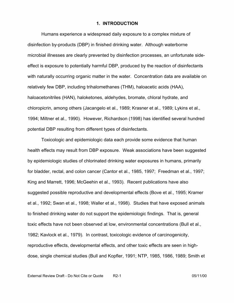
1. INTRODUCTION
Humans experience a widespread daily exposure to a complex mixture of
disinfection by-products (DBP) in finished drinking water. Although waterborne
microbial illnesses are clearly prevented by disinfection processes, an unfortunate side-
effect is exposure to potentially harmful DBP, produced by the reaction of disinfectants
with naturally occurring organic matter in the water. Concentration data are available on
relatively few DBP, including trihalomethanes (THM), haloacetic acids (HAA),
haloacetonitriles (HAN), haloketones, aldehydes, bromate, chloral hydrate, and
chloropicrin, among others (Jacangelo et al., 1989; Krasner et al., 1989; Lykins et al.,
1994; Miltner et al., 1990). However, Richardson (1998) has identified several hundred
potential DBP resulting from different types of disinfectants.
Toxicologic and epidemiologic data each provide some evidence that human
health effects may result from DBP exposure. Weak associations have been suggested
by epidemiologic studies of chlorinated drinking water exposures in humans, primarily
for bladder, rectal, and colon cancer (Cantor et al., 1985, 1997; Freedman et al., 1997;
King and Marrett, 1996; McGeehin et al., 1993). Recent publications have also
suggested possible reproductive and developmental effects (Bove et al., 1995; Kramer
et al., 1992; Swan et al., 1998; Waller et al., 1998). Studies that have exposed animals
to finished drinking water do not support the epidemiologic findings. That is, general
toxic effects have not been observed at low, environmental concentrations (Bull et al.,
1982; Kavlock et al., 1979). In contrast, toxicologic evidence of carcinogenicity,
reproductive effects, developmental effects, and other toxic effects are seen in high-
dose, single chemical studies (Bull and Kopfler, 1991; NTP, 1985, 1986, 1989; Smith et
External Review Draft - Do Not Cite or Quote R2-1 05/11/00
al., 1989). There is also evidence of mutagenicity from exposure to extracts of finished
drinking water in in vitro studies (Kool et al., 1981; Loper et al., 1978; Nestmann et al.,
1982). Although there are few studies available on defined mixtures of DBP, evidence
exists of dose-additivity for liver effects in mice exposed to mixtures of THM (Gennings
et al., 1997) and of promotion of cancer by mixtures of dichloroacetic acid (DCA) and
trichloroacetic acid (TCA) (Pereira et al., 1997).
Risk assessment questions surround the issues of establishing, explaining, and
estimating any substantive human health risks from exposure to the low levels of DBP
found in drinking water. Because toxic effects are not observed in animal studies when
the exposures are to low doses and because the epidemiologic data are inconsistent
across studies with only relatively weak associations noted, the existence of human
health risks is questionable, but cannot be entirely dismissed. If it is assumed, however,
that the human health effects suggested in epidemiologic studies are real, then several
hypotheses can be posed to explain the discrepancies between the epidemiologic
results and the lack of effects in animals exposed to finished drinking water. Such
hypotheses include: (1) there is an effect from exposure to the mixture of DBP that is at
least additive (if not synergistic) in nature, so that studies involving low levels of
individual DBP are inadequate to explain the health effects found in the positive
epidemiologic data; (2) effects in humans are due to the chronic, repetitive insult from
daily exposure to DBP mixtures; (3) animal studies differ from human exposures in
ways such as differences in physiology, biochemistry, anatomy, and life style factors
(e.g., high fat diets) that prevent them from demonstrating the same outcomes; (4)
laboratory studies to date expose the animals to only a single route, usually oral, so that
External Review Draft - Do Not Cite or Quote R2-2 05/11/00
effects due to dermal or inhalation exposure are not observed; (5) effects in
epidemiologic studies are due to exposure to other environmental factors such as
metals and inorganic materials in the drinking water or concurrent exposures to
industrial pollutants in urban areas or pesticides in agricultural areas so that animal
studies solely focused on DBP will not corroborate epidemiologic findings.
Testing of these hypotheses is a useful approach for investigating the potential
risks from exposure to mixtures of DBP; studies can be designed to address these
hypotheses. These hypotheses also have implications for the way risk assessments
are performed for comparisons across drinking water treatment technologies. Such
hypotheses suggest that traditional methods that characterize “safe levels” for single
chemicals by individual routes are likely to underestimate risk from exposure to the
complex mixture. The inadequacies of such methods are numerous. They fail to
examine potential risk from exposure to multiple chemicals (DBP, as well as pesticides,
metals, etc.). They neglect to account for interaction effects among chemicals or for
decreased thresholds for effects that occur as a result of a total mixture dose, rather
than an individual chemical dose. They do not account for risk due to simultaneous
multiple route exposures (oral, dermal, and inhalation). They fail to provide a range of
risk estimates that reflect multiple toxicity data sets, considerations of mechanism, or
both animal and epidemiologic data. They do not consider the impact of the constant
daily human exposure to finished drinking water, nor do they take into account human
activity patterns that influence exposure. These particular concerns have caused risk
assessors to focus on methods that are novel and are able to account for more
variables than just a single chemical exposure that may be influencing risk.
External Review Draft - Do Not Cite or Quote R2-3 05/11/00
The U.S. EPA has developed a Comparative Risk Framework Methodology
(CRFM) and Case Study (U.S. EPA, 1998) that presents a method for evaluating the
cost-effectiveness of drinking water treatment technologies relative to the health
consequences incurred by their utilization. Human health endpoints of concern include
gastrointestinal illness and death from exposure to pathogens, as well as cancer illness
and death, and reproductive and developmental effects from exposure to DBP. The
case study was developed to illustrate that the CRFM is feasible to implement. Within
the case study, a mixtures risk assessment approach (i.e., response addition) was
employed to estimate risk from exposure to the DBP for only the oral route of exposure.
A Monte Carlo simulation provided for endpoint-specific distributions of risk estimates
that included some sources of uncertainty and also incorporated the variability of human
tap water consumption rates.
The motivation behind producing this document was to explore the potential
world of available data and methodologies for improving the current approach in the
CRFM and to identify data gaps and future research needs in this subject area.
Chapter 2 of this report summarizes the CRFM approach. In this chapter, NCEA-Cin
scientists and contractors presented an overview of the CRFM for the workshop
participants and attendees. (The full pre-meeting report for the workshop is contained
in Appendix I.) Chapter 3 summarizes the presentations by the multi-disciplinary group
of scientists involved in the workshop. These scientists explored alternative methods
for exposure, dose-response assessment and risk characterization and their potential
application to DBP mixtures. Chapter 4 presents a synopsis of the two days of brain-
storming and discussion by various “breakout” groups. These groups tackled the eight
External Review Draft - Do Not Cite or Quote R2-4 05/11/00

questions posed in the Charge to the Workshop Participants. Herein recommendations
for future applications and future methodological developments are made.
External Review Draft - Do Not Cite or Quote R2-5 05/11/00
2. CRFM: CURRENT DATA AND METHODS
2.1. PRESENTATION: OVERVIEW OF RISK ASSESSMENT OBJECTIVES: PRESENT THEORY AND CURRENT EQUATION FOR ESTIMATION OF DBP MIXTURES USING RESPONSE ADDITION (L.K. Teuschler)
The EPA has developed a CRFM for the comparison of health risks resulting
from exposure to disinfection by-products (DBP) and microbes in drinking water.
Human exposure to DBP in drinking water can be characterized as multiple chemical,
multiple route, low-level, and highly variable. Although human health effects resulting
from these exposures are uncertain, epidemiologic and toxicologic data suggest a
concern for several endpoints including cancer, and developmental and reproductive
effects. In order to compare DBP chemical risks within the CRFM, EPA needs to make
central tendency risk estimates with probability distributions for each of these endpoints
of concern.
Figure 2-1 shows an overview of the CRFM that combines the NAS Risk
Assessment Paradigm methodology with a public health approach, a Cost-Effectiveness
Analysis, to evaluate new drinking water treatment technologies in light of the gains in
health units relative to the cost in dollars to achieve those gains. The disparate health
endpoints for comparison include cancer illness and death, and developmental and
reproductive effects for disinfection by-products and gastrointestinal illness and mortality
for microbial exposures. The CRFM goes further than just estimating risks utilizing the
paradigm and develops a common health metric for use in making risk comparisons
between DBP and microbes (e.g., Cryptosporidium infections). In order to illustrate the
CRFM, the Agency has developed a case study. Figure 2-2 highlights the exposure
conditions and the use of the paradigm for chemical
External Review Draft - Do Not Cite or Quote R2-6 05/11/00
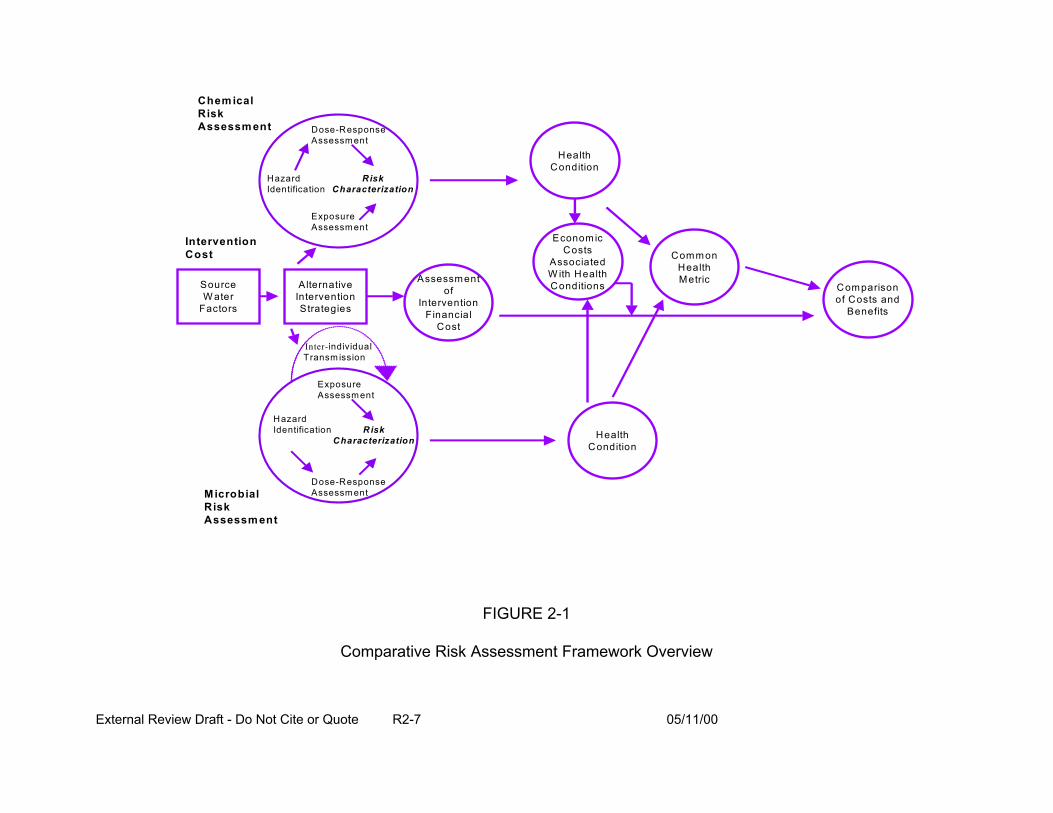
Chem ical
Altern ative In terve ntio n Strate g ies
D ose-R esponse A ssessm ent
Hazard Identification
Exposure A ssessm ent
Risk Characterization
D ose-R esponse A ssessm ent
Hazard Identification
Exposure A ssessm ent
Risk Ch aracterizatio n
Risk A ssess m en t
M icro b ial
Health C ondition
Health C ondition
C o mmon H ealth Me tric
T ransm ission In te r-individual
In terven tio n Co st
A s se ss m e n t of
In te rven tion F ina ncia l
Co st
E c onom ic Co sts
A ss o ciated W ith H ealth C o nd itio n sS ource
W a te r Factors
C o m parison of C o sts an d
B enefits
RiskAssessm ent
FIGURE 2-1
Comparative Risk Assessment Framework Overview
External Review Draft - Do Not Cite or Quote R2-7 05/11/00
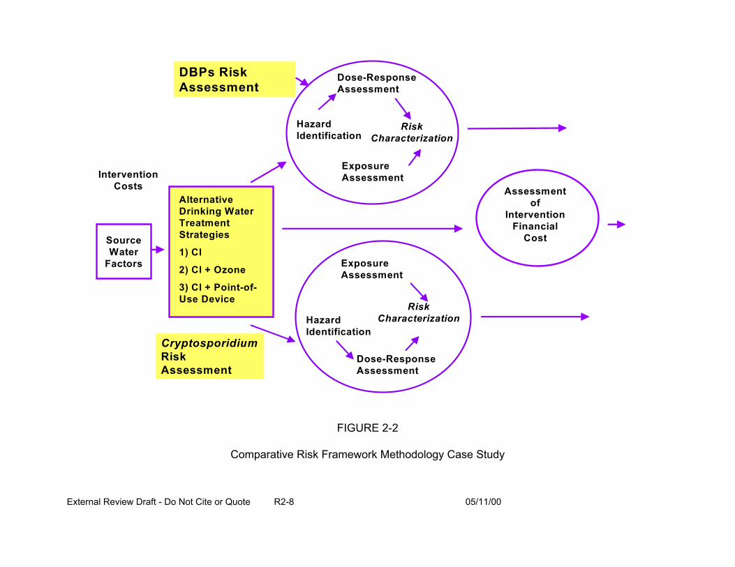
Assessment of
Intervention Financial
Cost
Dose-Response Assessment
Hazard Identification
Exposure Assessment
Risk Characterization
DBPs Risk Assessment
Cryptosporidium Risk Assessment
Intervention Costs
Alternative Drinking Water Treatment Strategies
1) Cl
2) Cl + Ozone
3) Cl + Point-of-Use Device
Dose-Response Assessment
Hazard Identification
Exposure Assessment
Risk Characterization
Source Water
Factors
FIGURE 2-2
Comparative Risk Framework Methodology Case Study
External Review Draft - Do Not Cite or Quote R2-8 05/11/00
risks in the case study that are the focus of the current workshop. In the illustrative
case study, the alternative drinking water treatment disinfection strategies that are
compared are: (1) filtration, post-chlorination; (2) pre-ozonation, filtration, post-
chlorination; and (3) filtration, post-chlorination, point-of-use device (e.g., an in-home
filter system).
The goals of the DBP risk estimation in the CRFM are to:
• compare DBP risks across drinking water treatment trains that reflect differences in which DBP are produced, as well as shifts in their concentration levels,
• make reasonable, useful risk estimates (other than zero) for all endpoints of concern because the epidemiologic and toxicologic evidence, although not conclusive, raise concern for cancer, and developmental and reproductive effects that need to be represented in the CRFM,
• develop distributions of risks in addition to central tendency estimates (not conservative, high-end estimates) that reflect their uncertainty and variability for use in the Monte Carlo and sensitivity analyses, and
• incorporate information on both the measured and unmeasured DBP into the risk estimate, as approximately 60% of the DBP in drinking water are represented only as summary measures (e.g., total organic halides) and are not identified as single chemicals.
A number of factors contribute to DBP risk uncertainty. These include:
• stochastic uncertainty in bioassay data,
• extrapolation to human risk estimates from animal dose-response toxicity data (when epidemiologic data are not available),
• variation in the presence and concentrations of DBP in the drinking water,
• seasonal (and other) variations in source water conditions,
• variations in human drinking water intake, and other uses of water,
External Review Draft - Do Not Cite or Quote R2-9 05/11/00
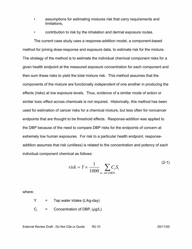
• assumptions for estimating mixtures risk that carry requirements and limitations,
• contribution to risk by the inhalation and dermal exposure routes.
The current case study uses a response-addition model, a component-based
method for joining dose-response and exposure data, to estimate risk for the mixture.
The strategy of the method is to estimate the individual chemical component risks for a
given health endpoint at the measured exposure concentration for each component and
then sum these risks to yield the total mixture risk. This method assumes that the
components of the mixture are functionally independent of one another in producing the
effects (risks) at low exposure levels. Thus, evidence of a similar mode of action or
similar toxic effect across chemicals is not required. Historically, this method has been
used for estimation of cancer risks for a chemical mixture, but less often for noncancer
endpoints that are thought to be threshold effects. Response-addition was applied to
the DBP because of the need to compare DBP risks for the endpoints of concern at
extremely low human exposures. For risk to a particular health endpoint, response-
addition assumes that risk (unitless) is related to the concentration and potency of each
individual component chemical as follows:
1 (2-1)risk = × ∑C SY i i1000 i All DBPs∈
where:
Y = Tap water intake (L/kg-day)
Ci = Concentration of DBPi (µg/L)
External Review Draft - Do Not Cite or Quote R2-10 05/11/00
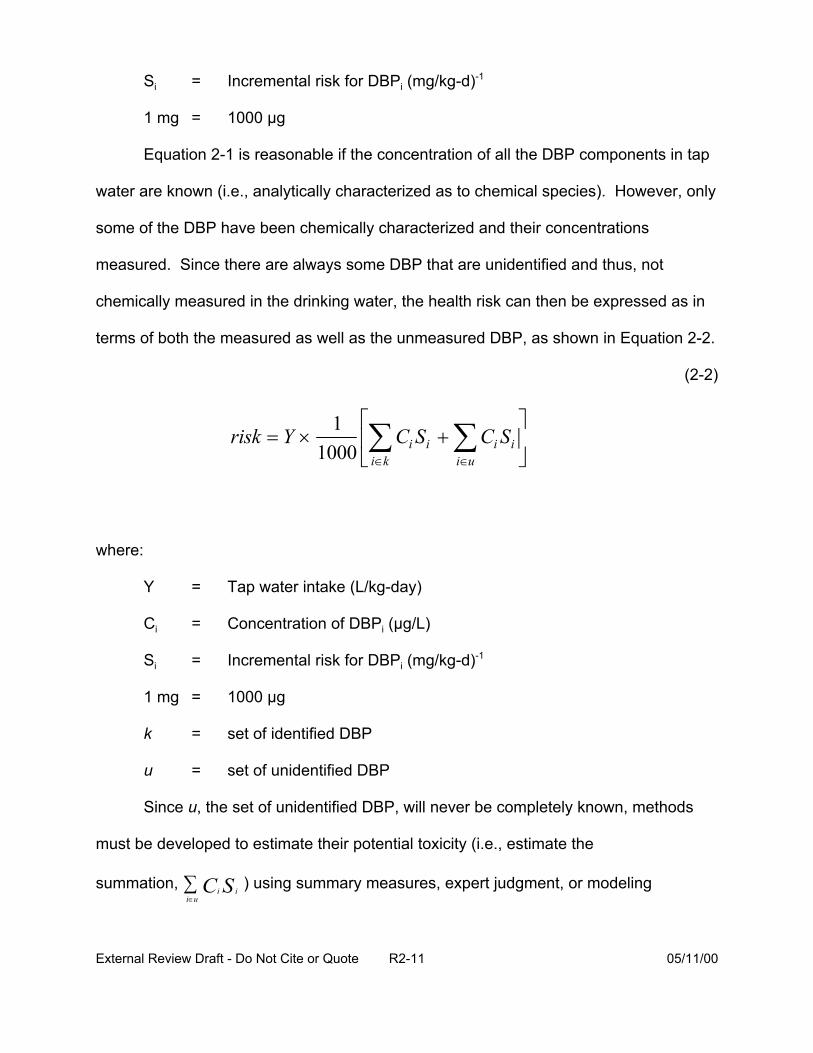
i ui k
Si = Incremental risk for DBPi (mg/kg-d)-1
1 mg = 1000 µg
Equation 2-1 is reasonable if the concentration of all the DBP components in tap
water are known (i.e., analytically characterized as to chemical species). However, only
some of the DBP have been chemically characterized and their concentrations
measured. Since there are always some DBP that are unidentified and thus, not
chemically measured in the drinking water, the health risk can then be expressed as in
terms of both the measured as well as the unmeasured DBP, as shown in Equation 2-2.
(2-2)
1 risk = × ∑C S +∑C SY i i i i 1000 ∈ ∈
where:
Y = Tap water intake (L/kg-day)
Ci = Concentration of DBPi (µg/L)
Si = Incremental risk for DBPi (mg/kg-d)-1
1 mg = 1000 µg
k = set of identified DBP
u = set of unidentified DBP
Since u, the set of unidentified DBP, will never be completely known, methods
must be developed to estimate their potential toxicity (i.e., estimate the
summation, ∑ C Si ) using summary measures, expert judgment, or modelingi i u∈
External Review Draft - Do Not Cite or Quote R2-11 05/11/00

i u i k
techniques. In the case study, it was assumed that the toxicity (or risk) for the
unidentified DBP associated with a health endpoint (e.g., developmental effects) is
equal to that of the identified DBP for the same health endpoint per unit of organic
halide (OX) concentration. That is, the risk from the unidentified components is
expressed in terms of the risk of the identified components of DBP, normalized by their
respective concentration of organic halides (in µg Cl/L), as shown in Equation 2-3.
oxCuH
oxCkH
(2-3)
∑C S ∑ C Si i i i ∈ ∈= ox oxCuH CkH
= organic halide (OX) concentration (in Fg Cl/L) of all unidentified DBP (H) associated with endpoint h
= corresponding concentration (in Fg Cl/L) for identified DBP (H) associated with endpoint h
Solving for the toxicity (risk) of the unidentified DBP associated with endpoint h,
this quantity can then be expressed as a fraction of the toxicity for the identified DBP,
based on their relative OX concentrations (Equation 2-4).
External Review Draft - Do Not Cite or Quote R2-12 05/11/00
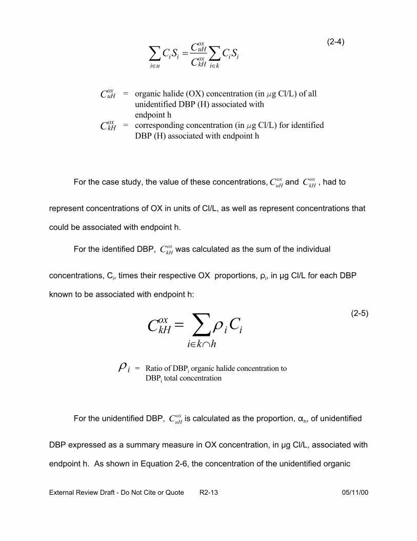
i k
i k
oxCuH
oxCkH
ox (2-4)
∑C S = CuH ∑C Si i ox i i i u CkH ∈∈
= organic halide (OX) concentration (in Fg Cl/L) of all unidentified DBP (H) associated with endpoint h
= corresponding concentration (in Fg Cl/L) for identified DBP (H) associated with endpoint h
ox oxFor the case study, the value of these concentrations, CuH and CkH , had to
represent concentrations of OX in units of Cl/L, as well as represent concentrations that
could be associated with endpoint h.
oxFor the identified DBP, CkH was calculated as the sum of the individual
concentrations, Ci, times their respective OX proportions, Di, in :g Cl/L for each DBP
known to be associated with endpoint h:
(2-5)oxCkH = ∑ρ Ci i ∈ ∩h
ρ i = Ratio of DBPi organic halide concentration to DBPi total concentration
oxFor the unidentified DBP, CuH is calculated as the proportion, " h, of unidentified
DBP expressed as a summary measure in OX concentration, in :g Cl/L, associated with
endpoint h. As shown in Equation 2-6, the concentration of the unidentified organic
External Review Draft - Do Not Cite or Quote R2-13 05/11/00
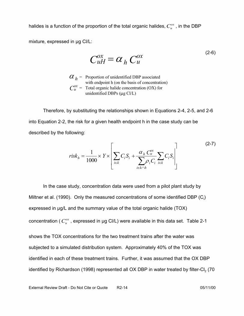
i k i k
i k
halides is a function of the proportion of the total organic halides, Cuox , in the DBP
mixture, expressed in :g Cl/L:
(2-6)ox oxCuH =α h Cu α h = Proportion of unidentified DBP associated
with endpoint h (on the basis of concentration)oxCu = Total organic halide concentration (OX) for
unidentified DBPs (:g Cl/L)
Therefore, by substituting the relationships shown in Equations 2-4, 2-5, and 2-6
into Equation 2-2, the risk for a given health endpoint h in the case study can be
described by the following:
(2-7) ox1 α h Curiskh =
1000 × Y ×
∑CiSi + ∑ρ C
∑C S
i i ∈ i i ∈ ∈ ∩h
In the case study, concentration data were used from a pilot plant study by
Miltner et al. (1990). Only the measured concentrations of some identified DBP (Ci)
expressed in :g/L and the summary value of the total organic halide (TOX)
concentration ( Cuox , expressed in :g Cl/L) were available in this data set. Table 2-1
shows the TOX concentrations for the two treatment trains after the water was
subjected to a simulated distribution system. Approximately 40% of the TOX was
identified in each of these treatment trains. Further, it was assumed that the OX DBP
identified by Richardson (1998) represented all OX DBP in water treated by filter-Cl2 (70
External Review Draft - Do Not Cite or Quote R2-14 05/11/00
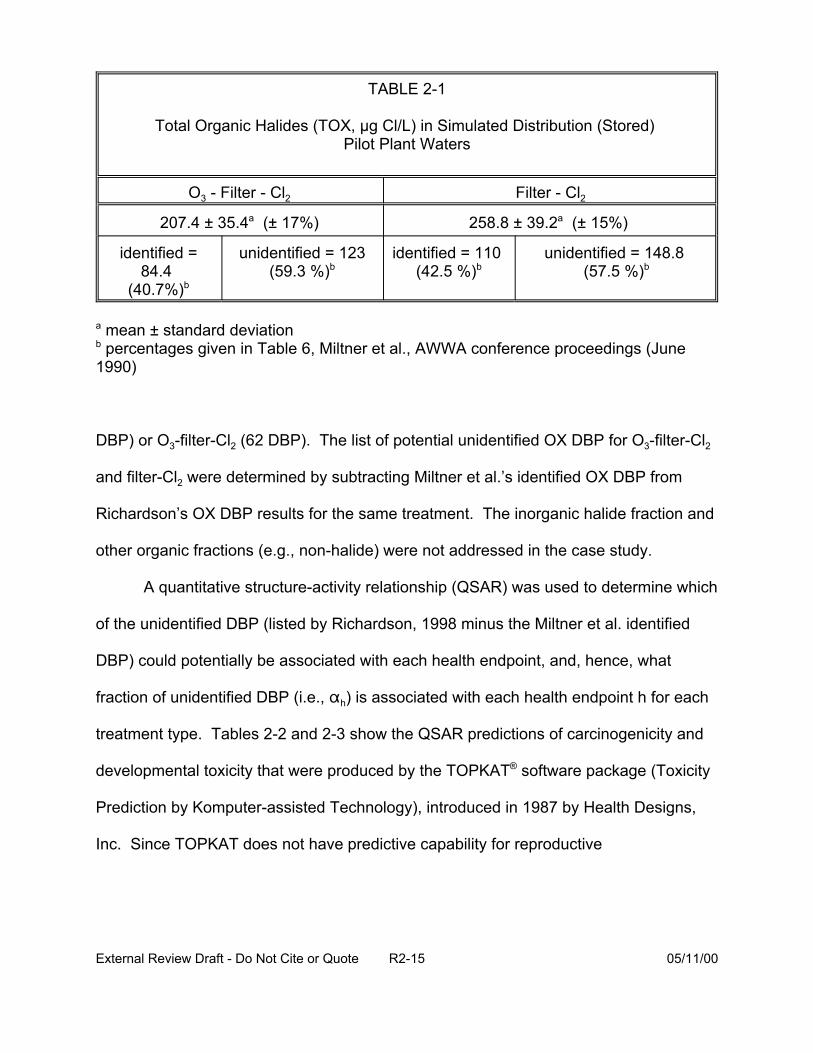
TABLE 2-1
Total Organic Halides (TOX, µg Cl/L) in Simulated Distribution (Stored) Pilot Plant Waters
O3 - Filter - Cl2 Filter - Cl2
207.4 ± 35.4a (± 17%) 258.8 ± 39.2a (± 15%)
identified = 84.4
(40.7%)b
unidentified = 123 (59.3 %)b
identified = 110 (42.5 %)b
unidentified = 148.8 (57.5 %)b
a mean ± standard deviationb percentages given in Table 6, Miltner et al., AWWA conference proceedings (June1990)
DBP) or O3-filter-Cl2 (62 DBP). The list of potential unidentified OX DBP for O3-filter-Cl2
and filter-Cl2 were determined by subtracting Miltner et al.’s identified OX DBP from
Richardson’s OX DBP results for the same treatment. The inorganic halide fraction and
other organic fractions (e.g., non-halide) were not addressed in the case study.
A quantitative structure-activity relationship (QSAR) was used to determine which
of the unidentified DBP (listed by Richardson, 1998 minus the Miltner et al. identified
DBP) could potentially be associated with each health endpoint, and, hence, what
fraction of unidentified DBP (i.e., " h) is associated with each health endpoint h for each
treatment type. Tables 2-2 and 2-3 show the QSAR predictions of carcinogenicity and
developmental toxicity that were produced by the TOPKAT® software package (Toxicity
Prediction by Komputer-assisted Technology), introduced in 1987 by Health Designs,
Inc. Since TOPKAT does not have predictive capability for reproductive
External Review Draft - Do Not Cite or Quote R2-15 05/11/00

TABLE 2-2
Chemical Class Total Developmental Total Cancer Cancer Female
Cancer Male Mouse
Cancer Female Rat
Cancer Male Rat
Aldehydes 0 1 1 0 0 0
Acids 3 5 4 2 3 0
Ketones 7 8 0 7 0 3
Lactones 0 3 1 1 1 0
Alcohols 0 1 0 1 0 0
Esters 1 1 0 0 0 1
Nitriles 4 2 1 0 1 0
Amides 0 0 0 0 0 0
Halo/Nitro Alkanes -Alkenes
3 2 7 5 6 6
Count / Total 18/43 33/57 - - - -
% Associated with Endpoint
42 58 - - - -
1
External Review Draft - Do Not Cite or Quote R2-16 05/11/00
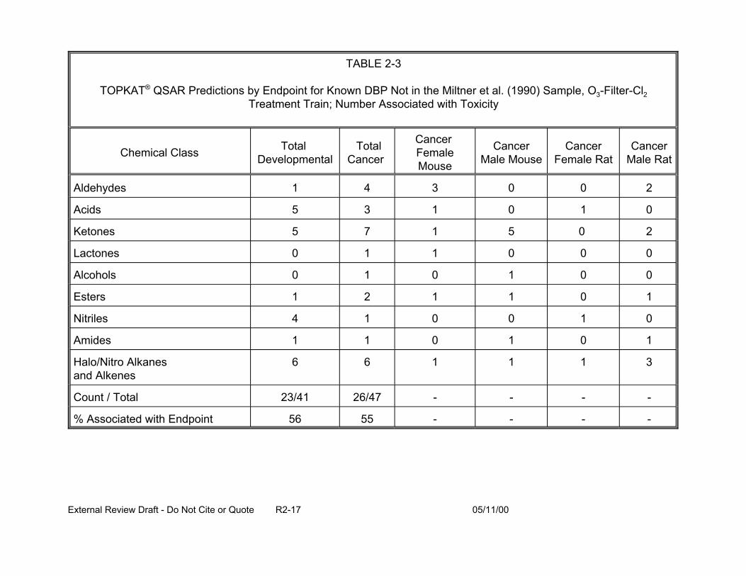
TABLE 2-3
TOPKAT® QSAR Predictions by Endpoint for Known DBP Not in the Miltner et al. (1990) Sample, O3-Filter-Cl2 Treatment Train; Number Associated with Toxicity
Chemical Class Total Developmental
Total Cancer
Cancer Female Mouse
Cancer Male Mouse
Cancer Female Rat
Cancer Male Rat
Aldehydes 1 4 3 0 0 2
Acids 5 3 1 0 1 0
Ketones 5 7 1 5 0
Lactones 0 1 1 0 0 0
Alcohols 0 1 0 1 0 0
Esters 1 2 1 1 0 1
Nitriles 4 1 0 0 1 0
Amides 1 1 0 1 0 1
Halo/Nitro Alkanes and Alkenes
6 1 1 1 3
Count / Total 23/41 26/47 - - - -
% Associated with Endpoint 56 55 - - - -
2
6
External Review Draft - Do Not Cite or Quote R2-17 05/11/00
endpoints, developmental predictions were used as a surrogate for reproductive effects.
Several important sources of uncertainty are recognized in this process. These include:
• Statistical models built into the TOPKAT® software may have introduced classification errors.
• The actual number and molecular weights of the chemicals that make up the unidentified DBP are unknown.
• The assumption that the toxicity of the unidentified DBP is the same as it is for the identified DBP when normalized in terms of OX concentration measured as :g Cl/L may be incorrect.
The EPA requested the experts’ assistance in: how to optimize use of all
available exposure, toxicity, and epidemiologic data to best characterize DBP risks
across drinking water treatment systems; how to better incorporate information on the
unidentified DBP into the risk assessment; identification of other QSAR models or
different toxicity measures than those generated by TOPKAT that could be used;
application of risk characterization methods that could be investigated based on
assumptions appropriate for the data; and recommendation of ways to characterize
uncertainty and variability.
2.2. PRESENTATION: OVERVIEW OF CHEMICAL EXPOSURE CONSIDERATIONS IN THE CASE STUDY OF THE U.S. EPA’S COMPARATIVE RISK FRAMEWORK METHODOLOGY (CRFM): ENGINEERING CONCERNS, SOURCE WATER CHARACTERISTICS, UNIDENTIFIED TOX, TAP WATER CONSUMPTION (G. Rice)
A goal of the illustrative case study in the draft CRFM (U.S. EPA, 1998) was to
facilitate a comparison among two hypothetical drinking water treatment systems. This
was accomplished by structuring the risk assessment/risk management interface
through construction of a transparent, decision analytic approach. Application of the
CRFM results in the comparison of cost-effectiveness ratios for each drinking water
External Review Draft - Do Not Cite or Quote R2-18 05/11/00
treatment system under consideration. The costs incurred through implementation of
the interventions form the numerator and the gain in public health associated with the
intervention is quantified in the denominator of the cost-effectiveness ratio. The
denominators of the cost-effectiveness ratios are based on risks posed by the
pathogens and the disinfection byproducts. In the case study of the CRFM, unbiased
estimates of the risks were quantified through application of the National Academy of
Science Risk Assessment Paradigm (NAS, 1983). For convenience, the risks analyzed
were limited to those posed by the disinfection by products and oocysts of the protozoal
parasite, Cryptosporidium parvum. The components of the DBP exposure assessment
developed in the limited case study as well as potentially important exposure
considerations not developed in the case study are described herein.
Exposure assessment consists of the evaluation of the magnitude, frequency,
duration, and route(s) of exposure. The risks posed by chemicals in drinking water can
be analyzed by aggregating exposure and effects, as is conducted in epidemiologic
investigation, by disaggregating exposure and effect and evaluating the components
independently, and then integrating them to assess risks (the approach taken in the
illustrative case study in the CRFM and described here). Alternatively, a hybrid
approach using both epidemiology (aggregation) and toxicology (disaggregation) can be
used.
2.2.1. Characteristics of the Source Water. Levels of DBP-precursors may be
variable across water bodies (e.g., bromide levels) or within water bodies (e.g., due to
climatological variation or seasonal changes in the patterns of water shed use). The
presence of other contaminants (biotic or abiotic) may influence the water treatment
External Review Draft - Do Not Cite or Quote R2-19 05/11/00
choice. Source water acidity or alkalinity or temperature influence the presence and
concentration of DBP in treated water. In the case study, the source water was drawn
from the Ohio River (Miltner et al., 1990, 1992). The temporal variability of DBP-
precursors in the source water was not analyzed and the impact of this variability on the
differences in the distribution of quantities and types of DBP formed between the
treatment systems being analyzed was not characterized.
2.2.2. Alternative Treatment Systems. The drinking water treatment system
alternatives impact the DBP levels in the treated drinking water. Factors that are
important in the selection of alternative drinking water treatment may include:
• feasibility,
• regulatory requirements, • acceptability of the intervention for legal or ethical reasons (e.g., a
community-based program mandating installation of in-home water filters in the homes of a sensitive subpopulations may be unacceptable),
• intervention cost, and
• anticipated benefits.
In the case study, two drinking water treatment systems were compared. The
baseline system consisted of coagulation, sedimentation, sand filtration, and chlorine
disinfection and the alternative system consisted of the baseline system supplemented
by a pre-ozonation step (Miltner et al., 1990; U.S. EPA, 1998).
2.2.3. Concentrations of DBP in Treated Waters: Distributions. Unbiased
estimates of the distributions of the quantities and types of DBP that form in the drinking
water treatment system are needed to characterize exposure. Ideally, these
concentrations will be measured at the taps over time. Data from Miltner et al. (1990,
1992) were used in the analysis (see Tables 2-4 and 2-5). The DBP were divided into
External Review Draft - Do Not Cite or Quote R2-20 05/11/00
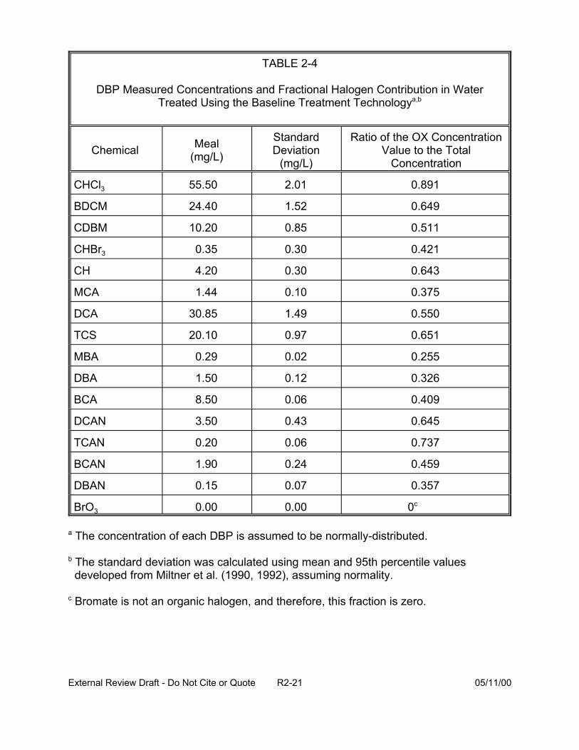
TABLE 2-4
DBP Measured Concentrations and Fractional Halogen Contribution in Water Treated Using the Baseline Treatment Technologya,b
Ratio of the OX Concentration Value to the Total
Concentration
0.891
BDCM 24.40 1.52 0.649
CDBM 10.20 0.85 0.511
CHBr3 0.35 0.30 0.421
CH 4.20 0.30 0.643
MCA 1.44 0.10 0.375
DCA 30.85 1.49 0.550
TCS 20.10 0.97 0.651
MBA 0.29 0.02 0.255
DBA 1.50 0.12 0.326
BCA 8.50 0.06 0.409
DCAN 3.50 0.43 0.645
TCAN 0.20 0.06 0.737
BCAN 1.90 0.24 0.459
DBAN 0.15 0.07 0.357
BrO3 0.00 0.00 0c
Chemical Meal (mg/L)
Standard Deviation
(mg/L)
CHCl3 55.50 2.01
a The concentration of each DBP is assumed to be normally-distributed.
b The standard deviation was calculated using mean and 95th percentile values developed from Miltner et al. (1990, 1992), assuming normality.
c Bromate is not an organic halogen, and therefore, this fraction is zero.
External Review Draft - Do Not Cite or Quote R2-21 05/11/00
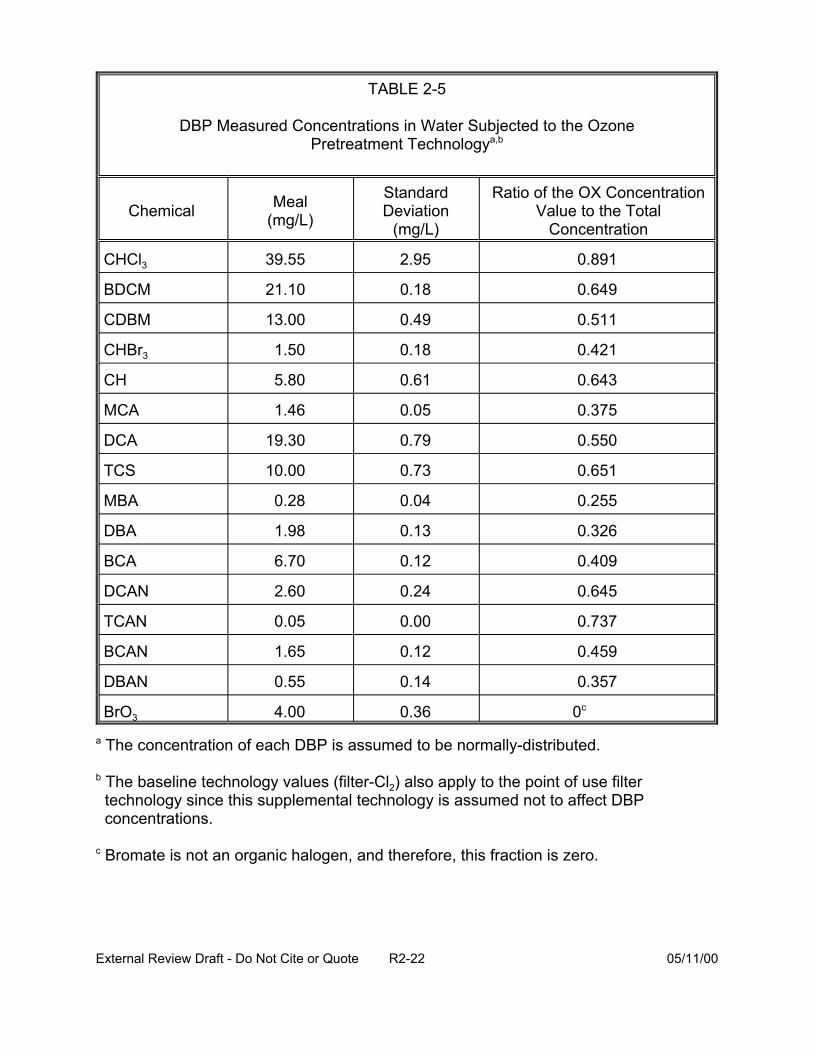
TABLE 2-5
DBP Measured Concentrations in Water Subjected to the Ozone Pretreatment Technologya,b
Ratio of the OX Concentration Value to the Total
Concentration
0.891
BDCM 21.10 0.18 0.649
CDBM 13.00 0.49 0.511
CHBr3 1.50 0.18 0.421
CH 5.80 0.61 0.643
MCA 1.46 0.05 0.375
DCA 19.30 0.79 0.550
TCS 10.00 0.73 0.651
MBA 0.28 0.04 0.255
DBA 1.98 0.13 0.326
BCA 6.70 0.12 0.409
DCAN 2.60 0.24 0.645
TCAN 0.05 0.00 0.737
BCAN 1.65 0.12 0.459
DBAN 0.55 0.14 0.357
BrO3 4.00 0.36 0c
Chemical Meal (mg/L)
Standard Deviation
(mg/L)
CHCl3 39.55 2.95
a The concentration of each DBP is assumed to be normally-distributed.
b The baseline technology values (filter-Cl2) also apply to the point of use filter technology since this supplemental technology is assumed not to affect DBP concentrations.
c Bromate is not an organic halogen, and therefore, this fraction is zero.
External Review Draft - Do Not Cite or Quote R2-22 05/11/00
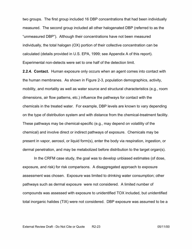
two groups. The first group included 16 DBP concentrations that had been individually
measured. The second group included all other halogenated DBP (referred to as the
“unmeasured DBP”). Although their concentrations have not been measured
individually, the total halogen (OX) portion of their collective concentration can be
calculated (details provided in U.S. EPA, 1999; see Appendix A of this report).
Experimental non-detects were set to one half of the detection limit.
2.2.4. Contact. Human exposure only occurs when an agent comes into contact with
the human membranes. As shown in Figure 2-3, population demographics, activity,
mobility, and mortality as well as water source and structural characteristics (e.g., room
dimensions, air flow patterns, etc.) influence the pathways for contact with the
chemicals in the treated water. For example, DBP levels are known to vary depending
on the type of distribution system and with distance from the chemical-treatment facility.
These pathways may be chemical-specific (e.g., may depend on volatility of the
chemical) and involve direct or indirect pathways of exposure. Chemicals may be
present in vapor, aerosol, or liquid form(s), enter the body via respiration, ingestion, or
dermal penetration, and may be metabolized before distribution to the target organ(s).
In the CRFM case study, the goal was to develop unbiased estimates (of dose,
exposure, and risk) for risk comparisons. A disaggregated approach to exposure
assessment was chosen. Exposure was limited to drinking water consumption; other
pathways such as dermal exposure were not considered. A limited number of
compounds was assessed with exposure to unidentified TOX included, but unidentified
total inorganic halides (TIX) were not considered. DBP exposure was assumed to be a
External Review Draft - Do Not Cite or Quote R2-23 05/11/00
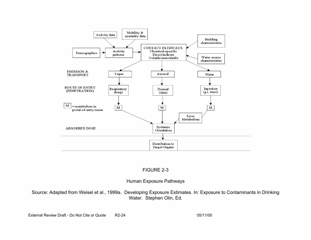
FIGURE 2-3
Human Exposure Pathways
Source: Adapted from Weisel et al., 1999a. Developing Exposure Estimates. In: Exposure to Contaminants in Drinking Water. Stephen Olin, Ed.
External Review Draft - Do Not Cite or Quote R2-24 05/11/00
function of total tap water consumed (L/kg-day). All water from the household tap
consumed directly as a beverage or used to prepare foods and beverages was
considered tap water. The studies of Ershow and Cantor (1989) of the U.S. population
and the Canadian Ministry of National Health and Welfare (1981), presented in U.S.
EPA (1997, Exposure Factors Handbook) were used to derive consumption estimates.
In addition, the Continuous Survey of Food Intake by Individuals (CSFII) data (1994-
1996) is currently undergoing evaluation within the EPA. The CRFM case study
quantified tap water consumption by fitting lognormal distributions to age-specific intake
data for the U.S. population developed by U.S. EPA (1997) based on Ershow and
Cantor (1989) and shown in Table 2-6. The water consumption of some subpopulations
was evaluated and found not to differ from the general population estimates. Because
reproductive and developmental effects induced by DBP are of concern, the water
consumption of pregnant women was evaluated. However, according to the data of
Ershow and Cantor (1989), the water consumption of pregnant women does not differ
from general population values. Therefore, no adjustment to consumption rates for this
subgroup in the CRFM was made. The AIDS population, however, has been reported
to drink significantly less tap water (Perz et al., 1998) than the general population. The
water consumption of this subgroup was adjusted downward in the case study. The
case study did not, however, evaluate exposure routes other than oral, compare
differences in DBP exposures from heated vs. unheated tap water, or account for
potential changes in consumption patterns (e.g., in CSFII increased use of bottled
water) since the time of data collection by Ershow and Cantor (1989).
External Review Draft - Do Not Cite or Quote R2-25 05/11/00
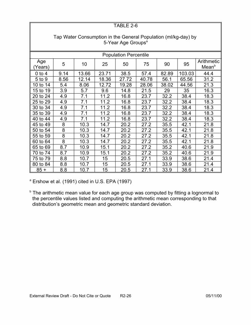
TABLE 2-6
Tap Water Consumption in the General Population (ml/kg-day) by 5-Year Age Groupsa
Population Percentile
5 10 52Age (Years) 50 75
0 to 4 9.14 13.66 23.71 38.5 57.4 5 to 9 8.56 12.14 18.36 27.72 40.78
10 to 14 19.28 28.06 15 to 19 14.8 21.5 20 to 24 16.8 23.7 25 to 29 16.8 23.7 30 to 34 16.8 23.7 35 to 39 16.8 23.7 40 to 44 16.8 23.7 45 to 49 20.2 27.2 50 to 54 20.2 27.2 55 to 59 20.2 27.2 60 to 64 20.2 27.2 65 to 69 20.2 27.2 70 to 74 20.2 27.2 75 to 79 20.5 27.1 80 to 84 20.5 27.1
85 + 20.5 27.1
0 95 Arithmetic Meanb
82.89 103.03 44.4 56.1 65.56 31.2
38.02 44.56 21.3 29 35 16.3
32.2 38.4 18.3 32.2 38.4 18.3 32.2 38.4 18.3 32.2 38.4 18.3 32.2 38.4 18.3 35.5 42.1 21.8 35.5 42.1 21.8 35.5 42.1 21.8 35.5 42.1 21.8 35.2 40.6 21.9 35.2 40.6 21.9 33.9 38.6 21.4 33.9 38.6 21.4 33.9 38.6 21.4
9
5.4 8.06 12.72 3.9 5.7 9.6 4.9 7.1 11.2 4.9 7.1 11.2 4.9 7.1 11.2 4.9 7.1 11.2 4.9 7.1 11.2 8 10.3 14.7 8 10.3 14.7 8 10.3 14.7 8 10.3 14.7
8.7 10.9 15.1 8.7 10.9 15.1 8.8 10.7 15 8.8 10.7 15 8.8 10.7 15
a Ershow et al. (1991) cited in U.S. EPA (1997)
b The arithmetic mean value for each age group was computed by fitting a lognormal to the percentile values listed and computing the arithmetic mean corresponding to that distribution’s geometric mean and geometric standard deviation.
External Review Draft - Do Not Cite or Quote R2-26 05/11/00
A central question posed to the experts was how the exposure assessment
approach used in the CRFM case study can be improved.
2.3. PRESENTATION: OVERVIEW OF TOXICOLOGY/CARCINOGENICITY ANIMAL DATA FOR USE IN QUANTITATIVE RISK ESTIMATION (J. Lipscomb)
The goal of extrapolating animal toxicity dose-response data to predict the
likelihood of adverse effects in humans is to use the best available toxicity data in the
risk assessment. For the DBP, this is complicated by many factors, including the
human exposure to low concentrations of these chemicals in treated drinking water and
the conducting of animals experiments at high doses of the same or closely related
chemicals. In addition, the question arises as to whether the critical effects observed in
animals are likely to be the same as the effects which are predicted to occur in the
humans.
Epidemiologic data for DBP have identified potential health outcomes of concern
(i.e., cancer, reproductive and developmental effects). A weak to moderate association
has been demonstrated between:
• low birth weight and consumption of chlorinated water,
• spontaneous abortions and bromodichloromethane (BDCM) exposure, and
• neural tube defects and exposure to trihalomethanes (THM).
Because the human data are uncertain and sparse, reproductive and
developmental toxicity and carcinogenicity data from peer-reviewed, published animal
studies were used to estimate health risks for the DBP. While hundreds of chemicals
have been identified as DBP in drinking water, chemicals applied in the case study were
restricted to those identified in the two treatment trains of interest and with available
External Review Draft - Do Not Cite or Quote R2-27 05/11/00
toxicity data for the human health points of concern. Other DBP that have toxicity data,
but were not shown to occur in the studies of Richardson (1998) or Miltner et al. (1990)
were excluded. The DBP that were identified in drinking water and met the above
criteria for inclusion in the case study are listed in Table 2-7.
2.3.1. Developmental and Reproductive Effects. The available animal
developmental toxicity data demonstrate multiple endpoints, primarily resorptions,
decreased live births, decreased crown-rump length, decreased body weight, heart
malformations, and eye malformations. Data availability restricted the consideration of
reproductive toxicity to that of direct effects on male reproductive endpoints. The
available studies for developmental and reproductive toxicity of the DBP comprise
primarily studies in rats treated by gavage, some with limitations in study design (e.g.,
maternal toxicity) or reporting of results.
In estimating risk for developmental and reproductive toxicity, a dose-response
model with a threshold parameter was applied to each endpoint within a study that
measured multiple endpoints (see Appendix A). Identified DBP toxicity data sets were
excluded when the model could not make reliable predictions or when the data sets
indicated a threshold effect for reproductive or developmental endpoints. The
Linearized Multi-Stage model was applied to available animal bioassay data to
determine “slope factors” or estimates of the potency for a given chemical. To avoid the
generation of point estimates of toxicity, a log normal distribution for the slope factors
was assumed. A surrogate approach was used to address the developmental toxicity
data gaps for dibromoacetic acid (DBA), bromochloroacetic acid (BCA), and
dibromoacetonitrile (DBAN) because available data indicated that developmental
External Review Draft - Do Not Cite or Quote R2-28 05/11/00
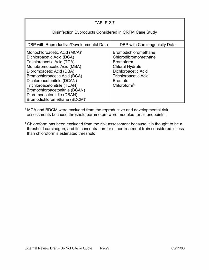
TABLE 2-7
Disinfection Byproducts Considered in CRFM Case Study
DBP with Reproductive/Developmental Data
Monochloroacetic Acid (MCA)a
Dichloroacetic Acid (DCA) Trichloroacetic Acid (TCA) Monobromoacetic Acid (MBA) Dibromoacetic Acid (DBA) Bromochloroacetic Acid (BCA) Dichloroacetonitrile (DCAN) Trichloroacetonitrile (TCAN) Bromochloroacetonitrile (BCAN) Dibromoacetonitrile (DBAN) Bromodichloromethane (BDCM)a
DBP with Carcinogenicity Data
Bromodichloromethane Chlorodibromomethane Bromoform Chloral Hydrate Dichloroacetic Acid Trichloroacetic Acid Bromate Chloroformb
a MCA and BDCM were excluded from the reproductive and developmental risk assessments because threshold parameters were modeled for all endpoints.
b Chloroform has been excluded from the risk assessment because it is thought to be a threshold carcinogen, and its concentration for either treatment train considered is less than chloroform’s estimated threshold.
External Review Draft - Do Not Cite or Quote R2-29 05/11/00
toxicity may be common for the haloacetic acid and haloacetonitrile DBP. The toxicity
and potency of dichloroacetic acid (DCA) was used as a surrogate for the toxicity and
potency of the haloacetic acids (HAA). Likewise, data for trichloroacetonitrile (TCAN)
were used as a surrogate for the haloacetonitriles (HAN). Tables 2-8 and 2-9 show the
incremental developmental toxicity risk for the identified DBP and the non-cancer dose-
response modeling results for DCA and trichloroacetic acid (TCA), respectively.
The incremental risk for reproductive toxicity for the three identified DBP for
which adequate data are available and the non-cancer dose-response modeling results
for DCA and DBA are shown in Tables 2-10 and 2-11, respectively.
2.3.2. Cancer. Epidemiologic studies have identified an association between the
ingestion of disinfected water and colorectal and bladder cancer in humans. Animal
bioassay data have shown evidence that several of the identified DBP are possible
human carcinogens (see Table 2-12). Site concordance between the human studies
and animal data is recognized as an issue for further deliberation. For the case study, it
was assumed that cancer risk in animals can be extrapolated to humans and that site
concordance was not a prerequisite. Slope factors were taken from EPA documents, or
verified by EPA Work Groups, except for those for TCA and DCA, which were classified
by EPA as C (possible human carcinogen) or B2 (probable human carcinogen),
respectively. Slope factors for DCA and TCA were calculated from the risk levels given
in Bull and Kopfler (1991). A lognormal distribution for the slope factors was assumed.
Unit risk values were recalculated using exposures as calculated in the case study (see
Section 2.2) and not using standard default values. Risk estimates for individual
External Review Draft - Do Not Cite or Quote R2-30 05/11/00
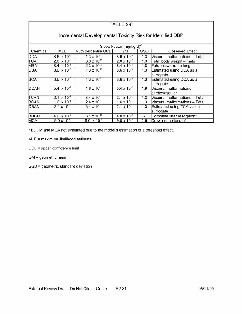
TABLE 2-8
Incremental Developmental Toxicity Risk for Identified DBP
Slope Factor (mg/kg-d)-1
Chemical MLE 95th percentile UCL GM GSD Observed Effect DCA 8.6 -3 1.3 x 10⁻² 8.6 x 10⁻³ 1.3 Visceral malformations – Total TCA 2.0 -2 3.0 x 10⁻² 2.0 x 10⁻² 1.3 Fetal body weight – male MBA 8.4 -3 2.3 x 10⁻² 8.4 x 10⁻³ 1.8 Fetal crown rump length DBA 8.6 -3 1.3 x 10⁻² 8.6 x 10⁻³ 1.3 Estimated using DCA as a
surrogate BCA 8.6 -3 1.3 x 10⁻² 8.6 x 10⁻³ 1.3 Estimated using DCA as a
surrogate DCAN 5.4 -2 1.6 x 10⁻¹ 5.4 x 10⁻² 1.9 Visceral malformations –
cardiovascular TCAN 2.1 -1 3.4 x 10⁻¹ 2.1 x 10⁻¹ 1.3 Visceral malformations – Total BCAN 1.6 -1 2.4 x 10⁻¹ 1.6 x 10⁻¹ 1.3 Visceral malformations – Total DBAN 2.1 x 10⁻¹ 3.4 x 10⁻¹ 2.1 x 10⁻¹ 1.3 Estimated using TCAN as a
surrogate BDCM 4.0 -2 3.1 x 10⁻² 4.0 x 10⁻² - Complete litter resorptiona
MCA 9.0 x 10⁻⁵ 6.0 -3 9.0 x 10⁻⁵ 2.6 Crown rump lengtha
x 10x 10x 10x 10
x 10
x 10
x 10x 10
x 10x 10
a BDCM and MCA not evaluated due to the model’s estimation of a threshold effect.
MLE = maximum likelihood estimate
UCL = upper confidence limit
GM = geometric mean
GSD = geometric standard deviation
External Review Draft - Do Not Cite or Quote R2-31 05/11/00
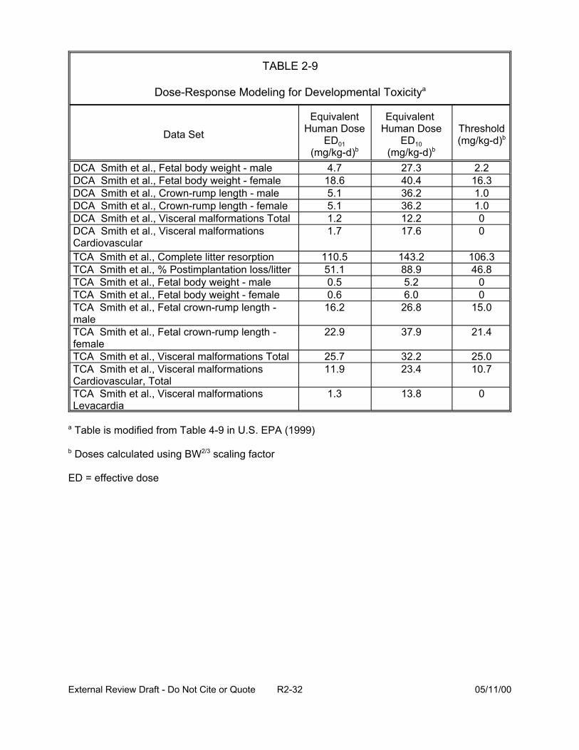
TABLE 2-9
Dose-Response Modeling for Developmental Toxicitya
Data Set
Equivalent Human Dose
ED01 (mg/kg-d)b
Equivalent Human Dose
ED10 (mg/kg-d)b
Threshold (mg/kg-d)b
4.7 27.3 2.2DCA DCA 18.6 40.4 16.3 DCA 5.1 36.2 1.0 DCA 5.1 36.2 1.0 DCA 1.2 12.2 0 DCA Cardiovascular
1.7 17.6 0
TCA 110.5 143.2 106.3 TCA 51.1 88.9 46.8 TCA 0.5 5.2 0 TCA 0.6 6.0 0 TCA male
16.2 26.8 15.0
TCA female
22.9 37.9 21.4
TCA 25.7 32.2 25.0 TCA Cardiovascular, Total
11.9 23.4 10.7
TCA Levacardia
1.3 13.8 0
Smith et al., Fetal body weight - male Smith et al., Fetal body weight - female Smith et al., Crown-rump length - male Smith et al., Crown-rump length - female Smith et al., Visceral malformations Total Smith et al., Visceral malformations
Smith et al., Complete litter resorption Smith et al., % Postimplantation loss/litter Smith et al., Fetal body weight - male Smith et al., Fetal body weight - female Smith et al., Fetal crown-rump length -
Smith et al., Fetal crown-rump length -
Smith et al., Visceral malformations Total Smith et al., Visceral malformations
Smith et al., Visceral malformations
a Table is modified from Table 4-9 in U.S. EPA (1999)
b Doses calculated using BW2/3 scaling factor
ED = effective dose
External Review Draft - Do Not Cite or Quote R2-32 05/11/00

TABLE 2-10
Incremental Reproductive Toxicity Risk for Identified DBP
Slope Factor (mg/kg-d)-1
Chemical MLE 95th percentile UCL GM GSD Observed Effect DBA 2.5 x 10⁻² 6.0 x 10⁻² 2.5 x 10⁻² 1.7 Number of cauda sperm
6.0 x 10⁻² 2.5 x 10⁻² 1.7 Estimated using DBA as aDCA 2.5 x 10⁻²
BCA 2.5 x 10⁻² 6.0 x 10⁻² surrogate
2.5 x 10⁻² 1.7 Estimated using DBA as a surrogate
MLE = maximum likelihood estimate
UCL = upper confidence limit
GM = geometric mean
GSD = geometric standard deviation
External Review Draft - Do Not Cite or Quote R2-33 05/11/00
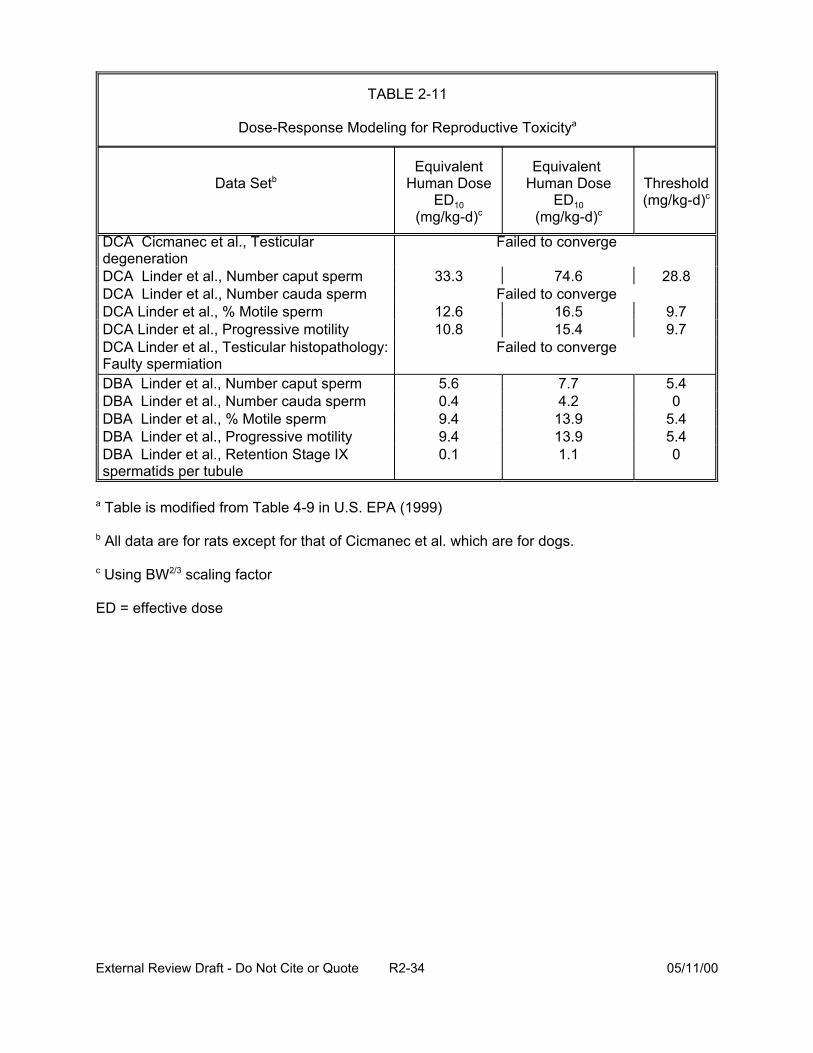
TABLE 2-11
Dose-Response Modeling for Reproductive Toxicitya
Data Setb Equivalent
Human Dose ED10
(mg/kg-d)c
Equivalent Human Dose
ED10 (mg/kg-d)c
Threshold (mg/kg-d)c
DCA Cicmanec et al., Testicular degeneration DCA Linder et al., Number caput sperm DCA Linder et al., Number cauda sperm DCA Linder et al., % Motile sperm DCA Linder et al., Progressive motility DCA Linder et al., Testicular histopathology: Faulty spermiation
Failed to converge
33.3 74.6 28.8 Failed to converge
12.6 16.5 9.7 10.8 15.4 9.7
Failed to converge
DBA Linder et al., Number caput sperm DBA Linder et al., Number cauda sperm DBA Linder et al., % Motile sperm DBA Linder et al., Progressive motility DBA Linder et al., Retention Stage IX spermatids per tubule
5.6 0.4 9.4 9.4 0.1
7.7 4.2
13.9 13.9 1.1
5.4 0
5.4 5.4 0
a Table is modified from Table 4-9 in U.S. EPA (1999)
b All data are for rats except for that of Cicmanec et al. which are for dogs.
c Using BW2/3 scaling factor
ED = effective dose
External Review Draft - Do Not Cite or Quote R2-34 05/11/00
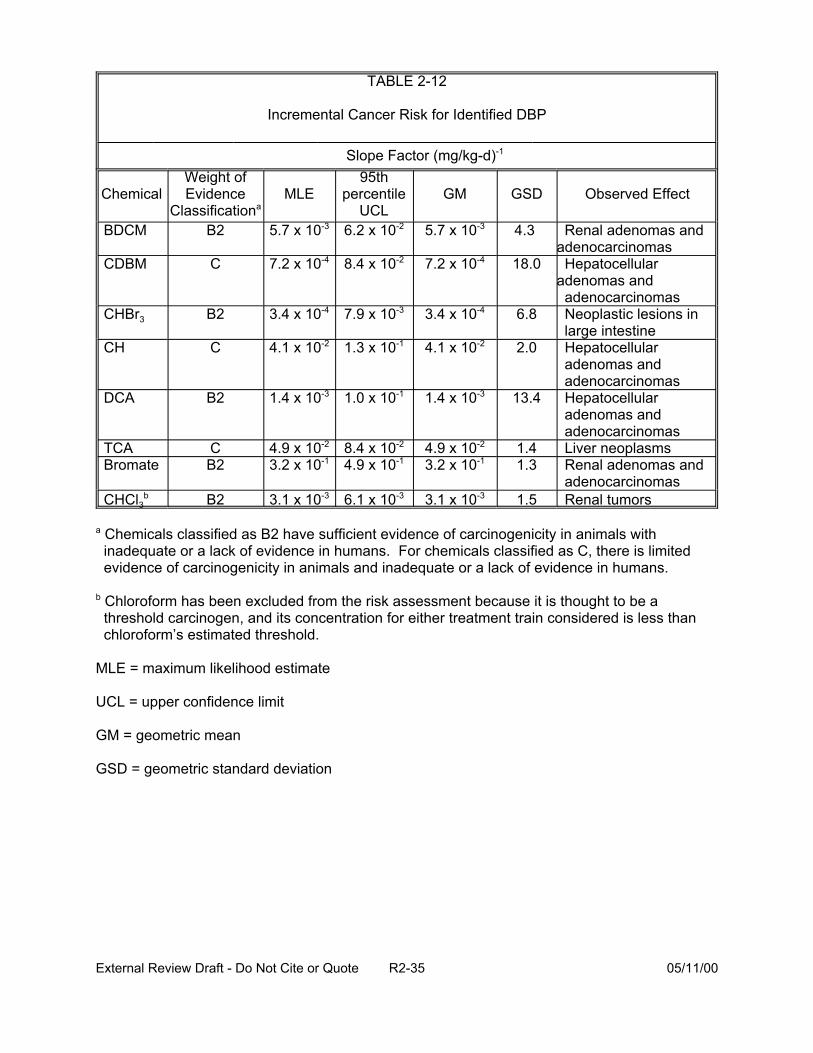
TABLE 2-12
Incremental Cancer Risk for Identified DBP
Slope Factor (mg/kg-d)-1
Chemical Weight of Evidence
Classificationa MLE
95th percentile
UCL GM GSD Observed Effect
BDCM B2 5.7 x 10⁻³ 6.2 x 10⁻² 5.7 x 10⁻³ 4.3 Renal adenomas and adenocarcinomas
CDBM C 7.2 x 10⁻⁴ 8.4 x 10⁻² 7.2 x 10⁻⁴ 18.0 Hepatocellular adenomas and adenocarcinomas
CHBr3 B2 3.4 x 10⁻⁴ 7.9 x 10⁻³ 3.4 x 10⁻⁴ 6.8 Neoplastic lesions in large intestine
CH C 4.1 x 10⁻² 1.3 x 10⁻¹ 4.1 x 10⁻² 2.0 Hepatocellular adenomas and adenocarcinomas
DCA B2 1.4 x 10⁻³ 1.0 x 10⁻¹ 1.4 x 10⁻³ 13.4 Hepatocellular adenomas and adenocarcinomas
TCA C 4.9 x 10⁻² 8.4 x 10⁻² 4.9 x 10⁻² 1.4 Liver neoplasms Bromate B2 3.2 x 10⁻¹ 4.9 x 10⁻¹ 3.2 x 10⁻¹ 1.3 Renal adenomas and
adenocarcinomas CHCl3
b B2 3.1 x 10⁻³ 6.1 x 10⁻³ 3.1 x 10⁻³ 1.5 Renal tumors
a Chemicals classified as B2 have sufficient evidence of carcinogenicity in animals with inadequate or a lack of evidence in humans. For chemicals classified as C, there is limited evidence of carcinogenicity in animals and inadequate or a lack of evidence in humans.
b Chloroform has been excluded from the risk assessment because it is thought to be a threshold carcinogen, and its concentration for either treatment train considered is less than chloroform’s estimated threshold.
MLE = maximum likelihood estimate
UCL = upper confidence limit
GM = geometric mean
GSD = geometric standard deviation
External Review Draft - Do Not Cite or Quote R2-35 05/11/00

chemicals were determined by multiplication of slope factors by the predicted intake
rates. Chloroform was excluded from the risk assessment because it is thought to have
a practical threshold and its concentration for either treatment train is less than
chloroform’s estimated threshold.
Issues for discussion by the experts were posed:
• Are there other DBP compounds that should be addressed?
• With respect to the data sets available, has the focus been on the critical health endpoints (toxicity) relevant to human health risk?
• Can multiple data sets be used quantitatively to producing the estimates of risk?
• Have reversibility and/or latency of effects been appropriately considered?
• Of what value would other approaches to quantifying rat reproductive effects be in this type assessment?
• Should epidemiologic findings be considered in a more quantitative fashion?
• Is the reliance upon the dose-response for effects produced by “surrogate” compounds appropriate?
• Is the assumption of a log normal distribution of slope factors appropriate?
• Should body weight be scaled to the 3/4 power instead of to the 2/3 power?
2.4. PRESENTATION: OVERVIEW OF AVAILABLE QUANTITATIVE EPIDEMIOLOGIC DATA: CANCER, DEVELOPMENTAL, REPRODUCTIVE ENDPOINTS (P. Murphy)
Some epidemiologic studies of chlorinated water and/or DBP, such as THM,
have suggested a weak to moderate association with various site-specific cancers
including bladder, colon, and rectum. The epidemiologic literature on adverse
reproductive and developmental outcomes is still very sparse and must be increased in
External Review Draft - Do Not Cite or Quote R2-36 05/11/00
both number and quality before quantitative use of the results can be entertained. The
reproductive and developmental endpoints evaluated in these studies are shown in
Table 2-13. The studies are described further in U.S. EPA (1998). In the CRFM, the
results from these studies could not be used quantitatively in the case study because
most of the exposure contrasts were confounded by water source and none of the
designs allowed for a comparison of the drinking water treatment practices of interest to
the current problem.
Each epidemiologic study was evaluated as to its internal validity (i.e., control for
confounding, selection bias, measurement error, and analytic errors and oversight) and
then in the context of the body of epidemiologic literature on chlorinated drinking
water/DBP. Following a determination of the validity of the individual studies, an
evaluation of both causal and noncausal explanations for the observed associations
was considered. General guidance for assessing causality in epidemiologic studies
includes evaluating the strength of the association, consistency, specificity, temporal
association, dose-response or biological gradient, biological plausibility, coherence of
findings, experimental evidence of preventability, and analogy. There are a number of
problems with the DBP epidemiological literature that make the studies difficult to
compare with one another. For example, in many of the reproductive and
developmental studies, the investigators have not always used the same operational
definitions for endpoints (such as low birth weight and spontaneous abortion) and
important confounding variables (occupational exposure, smoking, other risk factors)
have not been well-controlled.
External Review Draft - Do Not Cite or Quote R2-37 05/11/00
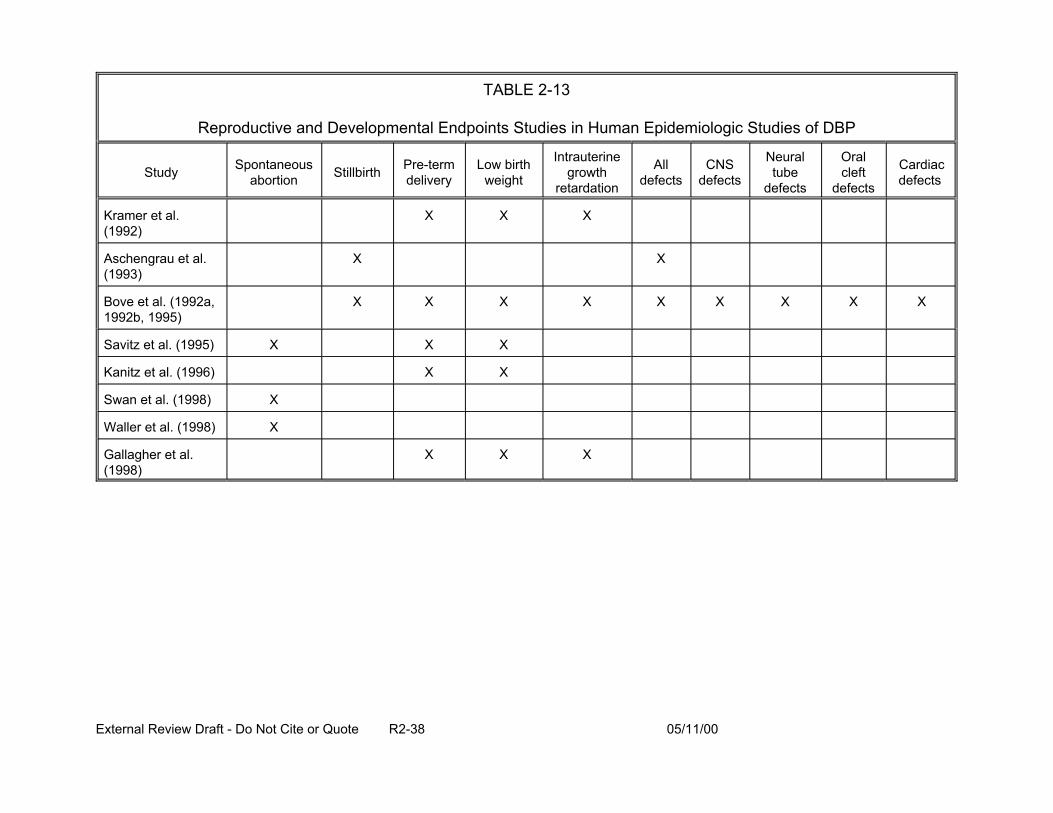
TABLE 2-13
Reproductive and Developmental Endpoints Studies in Human Epidemiologic Studies of DBP
Study Spontaneous abortion Stillbirth Pre-term
delivery Low birth
weight
Intrauterine growth
retardation
All defects
CNS defects
Neural tube
defects
Oral cleft
defects
Cardiac defects
Kramer et al. (1992)
X X X
Aschengrau et al. (1993)
X X
Bove et al. (1992a, 1992b, 1995)
X X X X X X X X X
Savitz et al. (1995) X X X
Kanitz et al. (1996) X X
Swan et al. (1998) X
Waller et al. (1998) X
Gallagher et al. (1998)
X X X
External Review Draft - Do Not Cite or Quote R2-38 05/11/00
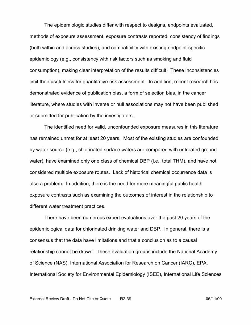
The epidemiologic studies differ with respect to designs, endpoints evaluated,
methods of exposure assessment, exposure contrasts reported, consistency of findings
(both within and across studies), and compatibility with existing endpoint-specific
epidemiology (e.g., consistency with risk factors such as smoking and fluid
consumption), making clear interpretation of the results difficult. These inconsistencies
limit their usefulness for quantitative risk assessment. In addition, recent research has
demonstrated evidence of publication bias, a form of selection bias, in the cancer
literature, where studies with inverse or null associations may not have been published
or submitted for publication by the investigators.
The identified need for valid, unconfounded exposure measures in this literature
has remained unmet for at least 20 years. Most of the existing studies are confounded
by water source (e.g., chlorinated surface waters are compared with untreated ground
water), have examined only one class of chemical DBP (i.e., total THM), and have not
considered multiple exposure routes. Lack of historical chemical occurrence data is
also a problem. In addition, there is the need for more meaningful public health
exposure contrasts such as examining the outcomes of interest in the relationship to
different water treatment practices.
There have been numerous expert evaluations over the past 20 years of the
epidemiological data for chlorinated drinking water and DBP. In general, there is a
consensus that the data have limitations and that a conclusion as to a causal
relationship cannot be drawn. These evaluation groups include the National Academy
of Science (NAS), International Association for Research on Cancer (IARC), EPA,
International Society for Environmental Epidemiology (ISEE), International Life Sciences
External Review Draft - Do Not Cite or Quote R2-39 05/11/00
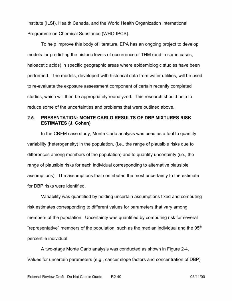
Institute (ILSI), Health Canada, and the World Health Organization International
Programme on Chemical Substance (WHO-IPCS).
To help improve this body of literature, EPA has an ongoing project to develop
models for predicting the historic levels of occurrence of THM (and in some cases,
haloacetic acids) in specific geographic areas where epidemiologic studies have been
performed. The models, developed with historical data from water utilities, will be used
to re-evaluate the exposure assessment component of certain recently completed
studies, which will then be appropriately reanalyzed. This research should help to
reduce some of the uncertainties and problems that were outlined above.
2.5. PRESENTATION: MONTE CARLO RESULTS OF DBP MIXTURES RISK ESTIMATES (J. Cohen)
In the CRFM case study, Monte Carlo analysis was used as a tool to quantify
variability (heterogeneity) in the population, (i.e., the range of plausible risks due to
differences among members of the population) and to quantify uncertainty (i.e., the
range of plausible risks for each individual corresponding to alternative plausible
assumptions). The assumptions that contributed the most uncertainty to the estimate
for DBP risks were identified.
Variability was quantified by holding uncertain assumptions fixed and computing
risk estimates corresponding to different values for parameters that vary among
members of the population. Uncertainty was quantified by computing risk for several
“representative” members of the population, such as the median individual and the 95th
percentile individual.
A two-stage Monte Carlo analysis was conducted as shown in Figure 2-4.
Values for uncertain parameters (e.g., cancer slope factors and concentration of DBP)
External Review Draft - Do Not Cite or Quote R2-40 05/11/00
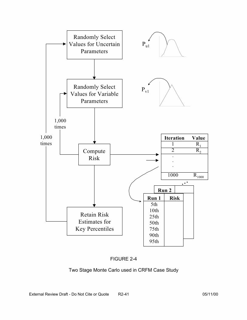
Run 2
Randomly Select Values for Uncertain
Parameters
Randomly Select Values for Variable
Parameters
Retain Risk Estimates for
Key Percentiles
Compute Risk
1,000 times
1,000 times
Pu1
Pv1
Iteration Value 1 1 2 2 . . .
1000 R1000
Run 1 Risk 5th
10th 25th 50th 75th 90th 95th
...
RR
FIGURE 2-4
Two Stage Monte Carlo used in CRFM Case Study
External Review Draft - Do Not Cite or Quote R2-41 05/11/00

were randomly selected and held constant, and then 1000 sets of values for the variable
parameters (e.g., water consumption, L-kg/day) were randomly drawn (corresponding to
1000 iterations of the inner loop) and used to compute 1000 estimates of risk. After
ranking the 1000 risk estimates from the inner loop, some key population summary
statistics estimates (i.e., 5th, 10th, 25th, 50th, 75th, 90th, and 95th percentiles) were retained
(Figure 2-5). The simulation then proceeded to the next iteration of the outer loop,
selecting new random values for the uncertain parameters and then executing 1000
new iterations of the inner loop. The outer loop was ultimately executed 1000 times,
yielding 1000 estimates of each of the key population summary statistic risk estimates.
For each health condition (cancer, developmental toxicity, and reproductive toxicity), the
set of parameters having the greatest influence on the determination of risk was
determined by modeling the population mean risk as a function of the uncertain
parameters using the following linear regression model:
a 2 2 +b3Vi3 +bViRi,50 = +b1Vi1 +bVi 4 4 +∈i (2-8)
where:
Vij = value for the jth parameter for simulation i,
Rij = risk for jth percentile of the population estimated for simulation i,
, = normally-distributed regression model
External Review Draft - Do Not Cite or Quote R2-42 05/11/00
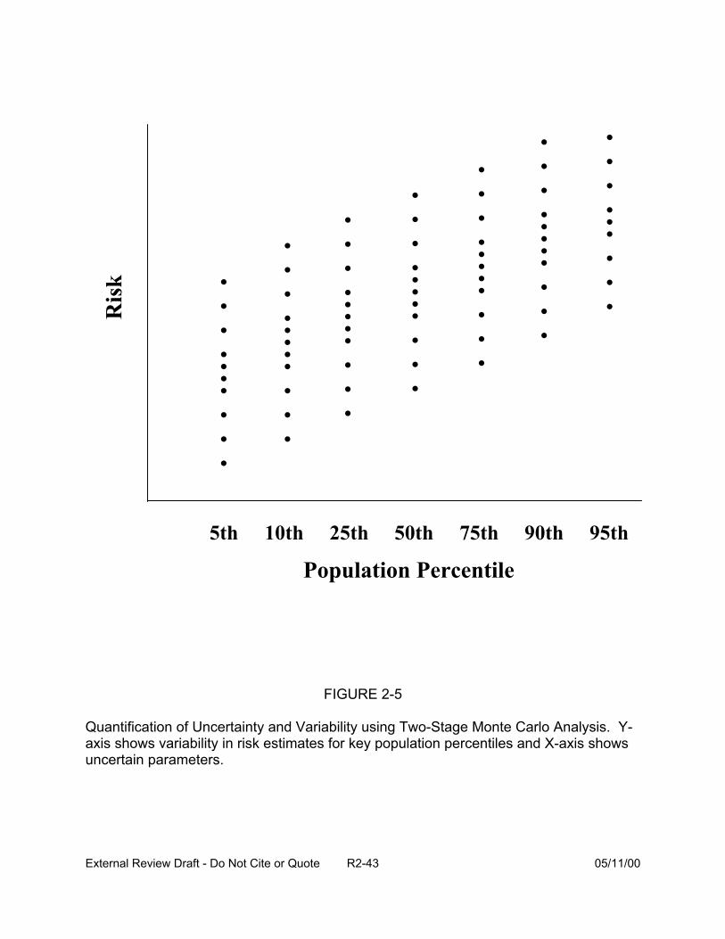
. . . . .. . . . .
. . . . .. .. . . .
. . . . .. . . .
. . . . .. . .. . .
. . . . . .. . . . .
. . . ... .. . . .
. . . . . ... . . .
5th 10th 25th 50th 75th 90th 95th
Population Percentile
FIGURE 2-5
Quantification of Uncertainty and Variability using Two-Stage Monte Carlo Analysis. Y-axis shows variability in risk estimates for key population percentiles and X-axis shows uncertain parameters.
Ris
k
External Review Draft - Do Not Cite or Quote R2-43 05/11/00
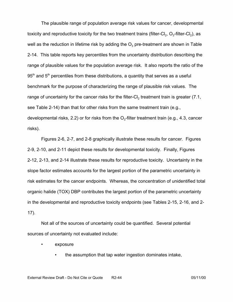
The plausible range of population average risk values for cancer, developmental
toxicity and reproductive toxicity for the two treatment trains (filter-Cl2, O3-filter-Cl2), as
well as the reduction in lifetime risk by adding the O3 pre-treatment are shown in Table
2-14. This table reports key percentiles from the uncertainty distribution describing the
range of plausible values for the population average risk. It also reports the ratio of the
95th and 5th percentiles from these distributions, a quantity that serves as a useful
benchmark for the purpose of characterizing the range of plausible risk values. The
range of uncertainty for the cancer risks for the filter-Cl2 treatment train is greater (7.1,
see Table 2-14) than that for other risks from the same treatment train (e.g.,
developmental risks, 2.2) or for risks from the O3-filter treatment train (e.g., 4.3, cancer
risks).
Figures 2-6, 2-7, and 2-8 graphically illustrate these results for cancer. Figures
2-9, 2-10, and 2-11 depict these results for developmental toxicity. Finally, Figures
2-12, 2-13, and 2-14 illustrate these results for reproductive toxicity. Uncertainty in the
slope factor estimates accounts for the largest portion of the parametric uncertainty in
risk estimates for the cancer endpoints. Whereas, the concentration of unidentified total
organic halide (TOX) DBP contributes the largest portion of the parametric uncertainty
in the developmental and reproductive toxicity endpoints (see Tables 2-15, 2-16, and 2-
17).
Not all of the sources of uncertainty could be quantified. Several potential
sources of uncertainty not evaluated include:
• exposure
• the assumption that tap water ingestion dominates intake,
External Review Draft - Do Not Cite or Quote R2-44 05/11/00
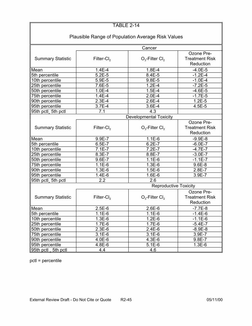
TABLE 2-14
Plausible Range of Population Average Risk Values
Cancer
Summary Statistic Filter-Cl2 O3-Filter Cl2
Ozone Pre-Treatment Risk
Reduction Mean 1.4E-4 1.8E-4 -4.0E-5 5th percentile 5.2E-5 8.4E-5 -1.2E-4 10th percentile 5.9E-5 9.8E-5 -1.0E-4 25th percentile 7.6E-5 1.2E-4 -7.2E-5 50th percentile 1.0E-4 1.5E-4 -4.6E-5 75th percentile 1.4E-4 2.0E-4 -1.7E-5 90th percentile 2.3E-4 2.6E-4 1.2E-5 95th percentile 3.7E-4 3.6E-4 4.5E-5 95th pctl¸ 5th pctl 7.1 4.3
Developmental Toxicity
Summary Statistic Filter-Cl2 O3-Filter Cl2
Ozone Pre-Treatment Risk
Reduction Mean 9.9E-7 1.1E-6 -9.9E-8 5th percentile 6.5E-7 6.2E-7 -6.0E-7 10th percentile 7.1E-7 7.2E-7 -4.7E-7 25th percentile 8.3E-7 8.8E-7 -3.0E-7 50th percentile 9.6E-7 1.1E-6 -1.1E-7 75th percentile 1.1E-6 1.3E-6 9.6E-8 90th percentile 1.3E-6 1.5E-6 2.8E-7 95th percentile 1.4E-6 1.6E-6 3.9E-7 95th pctl¸ 5th pctl 2.2 2.6
Reproductive Toxicity
Summary Statistic Filter-Cl2 O3-Filter Cl2
Ozone Pre-Treatment Risk
Reduction Mean 2.5E-6 2.6E-6 -7.7E-8 5th percentile 1.1E-6 1.1E-6 -1.4E-6 10th percentile 1.3E-6 1.2E-6 -1.1E-6 25th percentile 1.7E-6 1.7E-6 -5.4E-7 50th percentile 2.3E-6 2.4E-6 -8.9E-8 75th percentile 3.1E-6 3.1E-6 3.9E-7 90th percentile 4.0E-6 4.3E-6 9.8E-7 95th percentile 4.8E-6 5.1E-6 1.3E-6
4.4 4.695th pctl ¸ 5th pctl
pctl = percentile
External Review Draft - Do Not Cite or Quote R2-45 05/11/00
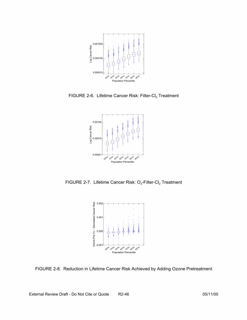
0.001000
Log
Can
cer R
isk
Log
Can
c er R
isk
0.000100
0.000010 H
1 H2 H
5 H7 H
9 H9 H50 T T0 T5 T0 T5 T0 T5
Population Percentile
FIGURE 2-6. Lifetime Cancer Risk: Filter-Cl2 Treatment
0.00100
0.00010
0.00001 H
1 H
2 H
5 H
7 H
9 H
9 H
50 T T0 T5 T0 T5 T0 T5
Population Percentile
FIGURE 2-7. Lifetime Cancer Risk: O3-Filter-Cl2 Treatment
Ozo
ne P
r e-T
x --
Dec
reas
ed C
ance
r Ris
k 0.002
0.001
0.000
-0.001 H
1 H
2 H
5 H
7 H
9 H
9 H
50 T T0 T5 T0 T5 T0 T5
Population Percentile
FIGURE 2-8. Reduction in Lifetime Cancer Risk Achieved by Adding Ozone Pretreatment
External Review Draft - Do Not Cite or Quote R2-46 05/11/00
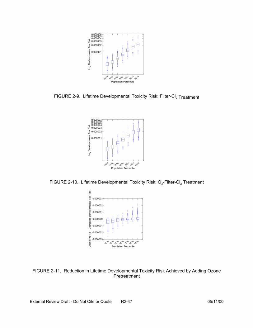
0.0000060.0000050.000004 0.000003 0.000002
0.000001
Log
Dev
elop
men
tal T
ox R
i sk
Log
Dev
leo p
men
tal T
ox R
isk
H1
H2
H5
H7
H9
H9
H50 T T0 T5 T0 T5 T0 T5
Population Percentile
FIGURE 2-9. Lifetime Developmental Toxicity Risk: Filter-Cl2 Treatment
0.0000070.0000060.0000050.000004 0.000003 0.000002
0.000001
H1
H2
H5
H7
H9
H9
H50 T T0 T5 T0 T5 T0 T5
Population Percentile
FIGURE 2-10. Lifetime Developmental Toxicity Risk: O3-Filter-Cl2 Treatment
Ozo
ne P
re-T
x --
Dec
reas
ed D
evel
opm
enta
l Tox
Ris
k
0.000003
0.000002
0.000001
0.000000
-0.000001
-0.000002
-0.000003 H
1 H
2 H
5 H
7 H
9 H
9 H
50 T T0 T5 T0 T5 T0 T5
Population Percentile
FIGURE 2-11. Reduction in Lifetime Developmental Toxicity Risk Achieved by Adding Ozone Pretreatment
External Review Draft - Do Not Cite or Quote R2-47 05/11/00
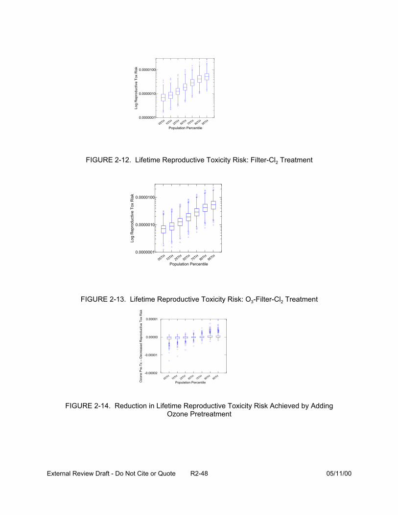
0.0000100
Log
Rep
rod u
ctiv
e To
x R
isk
Log
Rep
rodu
ctiv
e To
x R
isk
0.0000010
0.0000001 H
1 H2 H
5 H7 H
9 H9 H50 T T0 T5 T0 T5 T0 T5
Population Percentile
FIGURE 2-12. Lifetime Reproductive Toxicity Risk: Filter-Cl2 Treatment
0.0000100
0.0000010
0.0000001 H
1 H
2 H
5 H
7 H
9 H
9 H
50 T T0 T5 T0 T5 T0 T5
Population Percentile
FIGURE 2-13. Lifetime Reproductive Toxicity Risk: O3-Filter-Cl2 Treatment
Ozo
ne P
re-T
x --
Dec
rea s
ed R
epro
duct
ive
Tox
Ris
k
0.00001
0.00000
-0.00001
-0.00002 H
1 H
2 H
5 H
7 H
9 H
9 H
50 T T0 T5 T0 T5 T0 T5
Population Percentile
FIGURE 2-14. Reduction in Lifetime Reproductive Toxicity Risk Achieved by Adding Ozone Pretreatment
External Review Draft - Do Not Cite or Quote R2-48 05/11/00
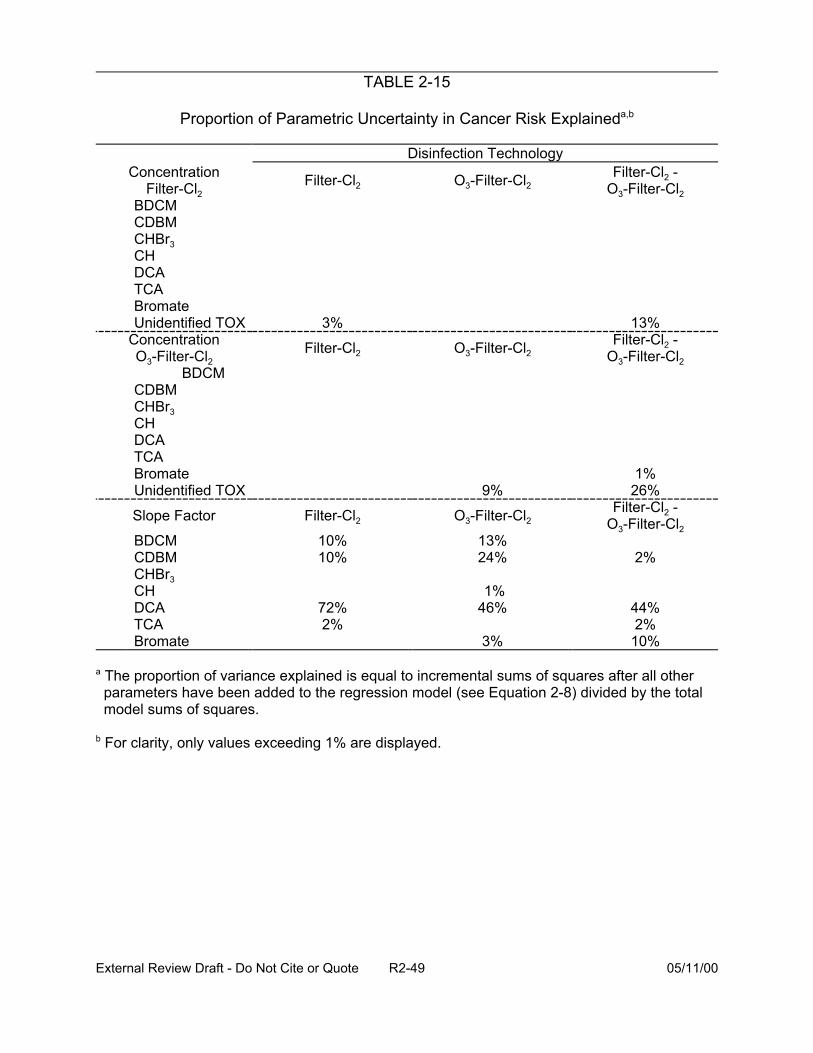
TABLE 2-15
Proportion of Parametric Uncertainty in Cancer Risk Explaineda,b
Disinfection Technology Concentration
Filter-Cl2 BDCM CDBM CHBr3 CH DCA TCA Bromate Unidentified TOX
Concentration O3-Filter-Cl2
BDCM CDBM CHBr3 CH DCA TCA Bromate Unidentified TOX
Slope Factor
BDCM CDBM CHBr3 CH DCA TCA Bromate
Filter-Cl2 -Filter-Cl2 O3-Filter-Cl2 O3-Filter-Cl2
3% 13% Filter-Cl2 -Filter-Cl2 O3-Filter-Cl2 O3-Filter-Cl2
1% 9% 26%
Filter-Cl2 O3-Filter-Cl2 Filter-Cl2 -
O3-Filter-Cl2 10% 13% 10% 24% 2%
1% 72% 46% 44% 2% 2%
3% 10%
a The proportion of variance explained is equal to incremental sums of squares after all other parameters have been added to the regression model (see Equation 2-8) divided by the total model sums of squares.
b For clarity, only values exceeding 1% are displayed.
External Review Draft - Do Not Cite or Quote R2-49 05/11/00
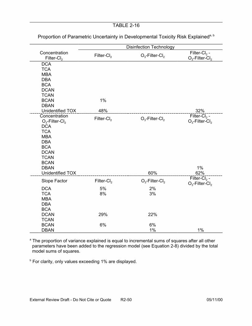
TABLE 2-16
Proportion of Parametric Uncertainty in Developmental Toxicity Risk Explaineda, b
Disinfection Technology
DCATCAMBADBABCADCANTCANBCANDBANUnidentified TOX
Concentration O3-Filter-Cl2 DCA TCA MBA DBA BCA DCAN TCAN BCAN DBAN Unidentified TOX
Slope Factor
DCA TCA MBA DBA BCA DCAN TCAN BCAN DBAN
Concentration Filter-Cl2Filter-Cl2
Filter-Cl2 -O3-Filter-Cl2 O3-Filter-Cl2
32% Filter-Cl2 -O3-Filter-Cl2 O3-Filter-Cl2
1% 60% 62%
Filter-Cl2 -O3-Filter-Cl2 O3-Filter-Cl2 2% 3%
22%
6% 1% 1%
1%
48%
Filter-Cl2
Filter-Cl2
5% 8%
29%
6%
a The proportion of variance explained is equal to incremental sums of squares after all other parameters have been added to the regression model (see Equation 2-8) divided by the total model sums of squares.
b For clarity, only values exceeding 1% are displayed.
External Review Draft - Do Not Cite or Quote R2-50 05/11/00
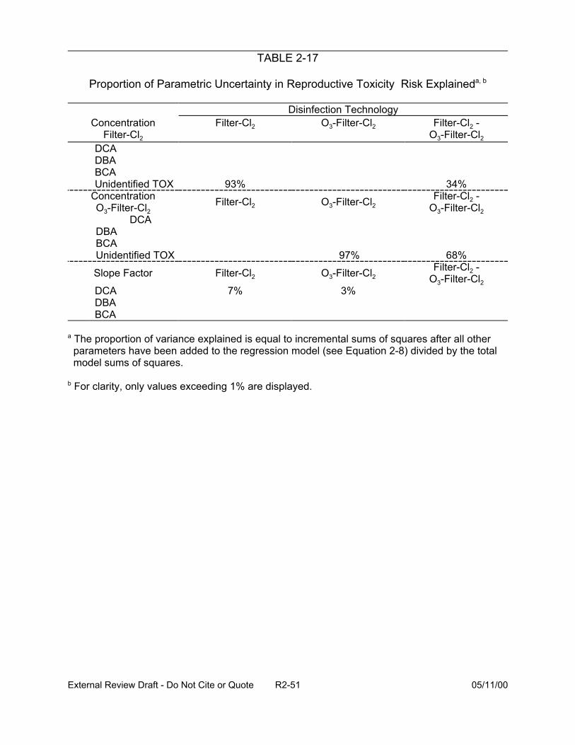
TABLE 2-17
Proportion of Parametric Uncertainty in Reproductive Toxicity Risk Explaineda, b
Disinfection Technology Concentration Filter-Cl2 O3-Filter-Cl2 Filter-Cl2 -
Filter-Cl2 O3-Filter-Cl2
DCADBABCAUnidentified TOX
ConcentrationO3-Filter-Cl2
DCA DBA BCA Unidentified TOX
Slope Factor
DCA DBA BCA
93% 34% Filter-Cl2 -Filter-Cl2 O3-Filter-Cl2 O3-Filter-Cl2
97% 68% Filter-Cl2 -Filter-Cl2 O3-Filter-Cl2 O3-Filter-Cl2
7% 3%
a The proportion of variance explained is equal to incremental sums of squares after all other parameters have been added to the regression model (see Equation 2-8) divided by the total model sums of squares.
b For clarity, only values exceeding 1% are displayed.
External Review Draft - Do Not Cite or Quote R2-51 05/11/00

• the use of total tap water intake value (rather than another estimate of tap water intake such as unheated tap water),
• toxicity
• use of QSAR to quantify the proportion of unidentified DBP associated with health endpoint, h (" h),
• the assumption that the unidentified DBP pose the same risk as the identified DBP on a :g OX/L basis,
• the assumption that chloroform is a threshold carcinogen,
• use of animal toxicity data to quantify the potency or slope factor (Si), and
• the assumption that the slope factors (Si) are statistically independent.
The exposure assumption that ingestion dominates intake could be important if
other routes of exposure result in much more efficient uptake or metabolism of the DBP.
Total tap water intake as the relevant measure of exposure is unlikely to be important as
shown by the uncertainty analysis. While there is some speculation that heating tap
water may remove some of the volatile DBP, restricting attention to the intake of only
unheated water affects the estimate of risk by at most a factor of 2, indicating that this
assumption is not a relatively important source of uncertainty.
The proportion of unidentified DBP associated with health endpoint, h (" h,) was
quantified using QSAR. Table 2-18 summarizes the impact of these extreme alternative
assumptions on the expected value of the population average risk. The range of risks
associated with the extreme alternative assumptions of 0% or 100% generally spanned
a factor of approximately 5 to 10, suggesting that this assumption does not substantially
contribute to uncertainty.
External Review Draft - Do Not Cite or Quote R2-52 05/11/00
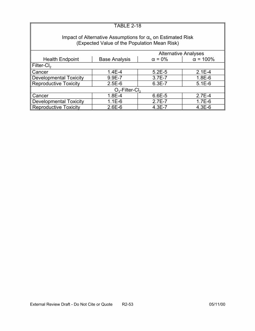
TABLE 2-18
Impact of Alternative Assumptions for " h on Estimated Risk (Expected Value of the Population Mean Risk)
Alternative Analyses Health Endpoint Base Analysis " = 0% " = 100%
Filter-Cl2
Cancer 1.4E-4 5.2E-5 2.1E-4 Developmental Toxicity 9.9E-7 3.7E-7 1.8E-6 Reproductive Toxicity 2.5E-6 6.3E-7 5.1E-6
O3-Filter-Cl2 Cancer 1.8E-4 6.6E-5 2.7E-4 Developmental Toxicity 1.1E-6 2.7E-7 1.7E-6 Reproductive Toxicity 2.6E-6 4.3E-7 4.3E-6
External Review Draft - Do Not Cite or Quote R2-53 05/11/00
The assumption that the unidentified DBP pose the same risk as the identified
DBP was evaluated by assuming alternatively that the unidentified DBP pose only 50%
the risk as the identified DBP (on a mg OX/L basis), and that the unidentified DBP pose
twice the risk as the identified DBP (on a mg OX/L basis) (Table 2-19). The results
indicate that this range of assumptions corresponds to a range of risk estimates
spanning a factor of approximately 5 to 10.
The assumption that chloroform is a threshold carcinogen affects the overall risks
by approximately 1.2 to 1.4, despite the assumption that the concentration of chloroform
is large and exceeds that of many of the other DBP. Whether or not chloroform is a
carcinogen at environmentally relevant exposure levels affects the cancer risk estimates
for two reasons. First, because the concentration of chloroform exceeds that of many
other DBP, its potential contribution to carcinogenicity is substantial. The assumption of
a threshold dose-response for carcinogenicity removes its contribution from the risk
estimate. Second, because chloroform’s concentration is large compared to that of
other DBP, its classification as a carcinogen affects the estimated risk associated with
exposure to unidentified DBP. Specifically, if it is not classified as a carcinogen, its
potency is removed from the weighted average used as an estimate of the typical
potency of an unidentified DBP. Since chloroform’s assumed potency is less than the
weighted average potency of the other identified DBP, removing it from consideration
(by assuming it does not behave as a carcinogen at environmentally relevant doses)
increases the weighted average potency of the set of identified DBP. These two
influences on risk work in the opposite direction and hence,
External Review Draft - Do Not Cite or Quote R2-54 05/11/00

TABLE 2-19
Impact of Alternative Assumptions for the Relative Toxicity of Unidentified DBP vs. Known DBP on Estimated Risk
(Expected Value of the Population Mean Risk)
Health Endpoint Base Analysis Alternative Analyses
Relative Tox = 50%
Relative Tox = 200%
Filter-Cl2
Cancer
Developmental Toxicity
Reproductive Toxicity
O-3-Filter-Cl2
Cancer
Developmental Toxicity
Reproductive Toxicity
1.9E-4
9.9E-7
2.5E-6
52.E-5 2.4E-4
3.7E-7 1.6E-6
6.3E-7 4.4E-6
6.6E-5 2.9E-4
2.7E-7 1.9E-6
1.8E-4
1.1E-6
2.6E-6 4.3E-7 4.8E-6
External Review Draft - Do Not Cite or Quote R2-55 05/11/00
partially cancel each other out. Assuming chloroform is a threshold carcinogen
decreases the total cancer potency of the identified DBP, but increases their potency on
a per mg OX/Cl basis, increasing the assumed potency of the unidentified DBP.
Risk estimates computed using the assumption that for each health endpoint, the
slope factors are perfectly correlated and do not differ substantially from the risk
estimates computed, with the assumption (used in the CRFM document) that these
quantities are statistically independent. This finding indicates that the assumption of
statistical independence is not an important source of uncertainty.
In place of the animal bioassay data used to quantify DBP carcinogenicity, the
epidemiology literature could be used. The following discussion estimates the
approximate degree to which the use of the epidemiology results would affect the
results of the risk assessment.
For the purpose of this analysis, attention is restricted to bladder and rectal
cancer. The SEER statistics data base reports the lifetime risk of disease for these
types of cancer:
• For bladder cancer, the lifetime risk is 2.27% (Ries et al., 1998, Table XXVI-8), although the risk for males is much higher (3.37%) than it is for females (1.17%);
• For colon and rectal cancer [get rectal only], the lifetime risk is 5.56% (Ries et al., 1998, Table VI-13).
Since the odds ratios for these diseases are not much greater than unity, the
incremental risk of disease can be estimated as the product of the population lifetime
risk and 1 minus the odds ratio. Dividing this incremental risk by total daily TOX intake
yields an estimate of the slope factor in (mg/kg-day)-1. In place of a measured dose
level, daily TOX intake is estimated here as the product of the average concentration for
External Review Draft - Do Not Cite or Quote R2-56 05/11/00
the Cl-filter treatment train (approximately 0.25 mg/L, Table 3.1-2, U.S. EPA, 1999) and
the arithmetic average daily tap water intake rate (0.022 L/kg-day1). Table 2-20
summarizes the calculation of the slope factor for bladder cancer and rectal cancer.
Assuming that these types of cancer represent the vast majority of the cancers caused
by exposure to disinfected drinking water, the slope factor for total TOX in disinfected
drinking water is the sum of the slope factors for these individual cancers. This slope of
4.7 (mg/kg-day)-1 can be compared to the animal bioassay-derived concentration-
weighted average slope factors for identified DBP. Using the mean DBP concentration
values as the weights, along with the slope values estimated from animal bioassay data
(Table 4-2, U.S. EPA, 1999) yields an average slope factor of 9 x 10⁻³ (mg/kg-day)-1 for
the filtration-chlorine train, and 1.8 x 10⁻² (mg/kg-day)-1 for the ozone-filtration-chlorine
treatment train. Therefore, the epidemiologically-derived slope factor exceeds the
animal bioassay derived averages by more than 2 orders of magnitude. The risk
calculated using the epidemiologic information is approximately 500 times larger than
the risk determined from the animal data, supporting that the “suggestive” findings for
cancer from the epidemiologic data may be considered important and that the risk
estimated from the animal studies could be an underestimate.
2.6. PARTICIPANT DISCUSSION: CURRENT DATA AND METHODOLOGIES
The participants noted that the context of use of the epidemiologic data in the
CRFM case study differs from the usual epidemiologic context. In the case study, the
question is not whether there is solid evidence for causality, but whether the
1 The arithmetic mean is the proper summary statistic to use. Since risk is hypothesized to be linear in dose, the average risk for the population as a whole is equal to the risk for an individual whose consumption is equal to that of the average for the population. The average intake rate was calculated by averaging the arithmetic means of the lognormal intake rates calculated in U.S. EPA (1999, Section 3.2).
External Review Draft - Do Not Cite or Quote R2-57 05/11/00
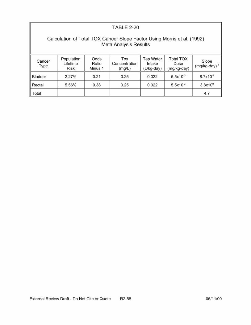
TABLE 2-20
Calculation of Total TOX Cancer Slope Factor Using Morris et al. (1992) Meta Analysis Results
Cancer Type
Population Lifetime
Risk
Odds Ratio
Minus 1
Tox Concentration
(mg/L)
Tap Water Intake
(L/kg-day)
Total TOX Dose
(mg/kg-day)
Slope (mg/kg-day)-1
Bladder 2.27% 0.21 0.25 0.022 5.5x10⁻³ 8.7x10⁻¹
Rectal 5.56% 0.38 0.25 0.022 5.5x10⁻³ 3.8x100
Total 4.7
External Review Draft - Do Not Cite or Quote R2-58 05/11/00
epidemiologic studies point to some probability, or a likely outcome. The indication of
adverse reproductive or developmental effects from epidemiologic data should not be
excluded.
The participants acknowledged the data gaps in research on DBP. It was noted
that there are a number of studies underway in animals regarding pharmacokinetics of
DBP. In addition, it was acknowledged that there are limitations in using gavage
animals studies (a bolus dose of a chemical in a vehicle which may also have an effect)
for predicting response in humans consuming tap water throughout the day. The
participants questioned why, in the comparison of risks with animal and epidemiologic
data, bladder cancer was chosen as there has been no comparable tumor seen in
animals studies. Kidney tumors in animal studies of the DBP may not be the most
relevant tumors for extrapolation to humans. It was suggested that gastrointestinal
tumors (i.e., colo-rectal tumors from the human studies and large intestine in animal
studies) might be more appropriate. The participants thought the question of the
necessity (or not) of site-concordance required further discussion during the breakout
sessions (Refer to Section 4).
The participants addressed the question of how the exposure assessment
approach in the CRFM could be improved. It was stated that examination of central
tendency and distribution of the whole population does not always provide information
on the subpopulation. For example, more recent information on pregnant women
suggests that consumption may increase during pregnancy. Consumption also varies
based on activity (e.g., recreation, exercise) and time at residence (consumption at
home vs. at work). It was noted that CSFII addresses some concerns about
External Review Draft - Do Not Cite or Quote R2-59 05/11/00
consumption information for subpopulations. For example, consumption data are
segregated by age, geography, race, pregnancy, lactating women, and socio-economic
status in the survey. The CSFII also reports consumption data for bottled water, soda,
tea, and coffee. It was noted that chemical constituents present in bottled water are
often not known; some bottled water is treated. The participants reiterated that the
presence and concentration of DBP varies based on numerous factors including the
source, storage and distribution systems and the influence of biota (may breakdown
organic halides). There are daily and seasonal changes in the concentration of DBP
both at the tap and throughout the treatment train. There are some studies in progress
on the effect of heating water on the concentrations of DBP. Additional research needs
be designed to look at chemical constituents, exposure differences and to make
comparisons at points throughout the water distribution system (Section 4.1 discusses
these points in more depth).
In response to the question posed by EPA as to how to incorporate information
on the unidentified DBP into the risk assessment, the participants felt that the
assumption that the unidentified DBP pose the same risk as the identified DBP is a big
assumption. There is also uncertainty in that there may be a correlation between
concentration of constituents and daily intake (e.g., a high concentration may reduce the
intake due to taste, odor aversion). It was noted that Richardson (1998) did not identify
all the chemicals in drinking water. The TIX may be closer in approximating the toxicity
of the DBP than the TOX. The unidentified DBP may be high molecular weight, polar
compounds such as pesticides or solvents, that could be more toxic than the TOX. The
mean of the TOX should be included as well as the median when showing results as it
External Review Draft - Do Not Cite or Quote R2-60 05/11/00
is a useful descriptor. Section 4.2 presents the breakout group discussion of the
unidentified constituents.
It was noted that it is the assumptions that are driving the sensitivity analysis in
the CRFM (i.e., the results may be an artifact of the assumptions). The model used to
determine parameters having the greatest influence on the determination of risk
(Equation 2-8) is very strongly linear and may overlook nonlinear components that
explain the risk. The point was made that one needs a better understanding of the
epidemiology data to better explain the variance. It was acknowledged that there is a
lot of uncertainty not being captured by the Monte Carlo analysis. These points are
further discussed in Section 4.
External Review Draft - Do Not Cite or Quote R2-61 05/11/00

3. NOVEL METHODS FOR MIXTURES
3.1. PRESENTATION: DOSE-RESPONSE MODELING IMPROVEMENTS: CANCER (D. Hattis)
Knowledge of the process of cancer, defined here as the end result of a
sequence of heritable changes in somatic cells, provides support for the assumption of
low-dose linearity in risk assessment. Genetic modes of action where the chemical or
agent reacts directly with DNA is based on bimolecular reaction kinetics as well as
pharmacokinetic processes (i.e., Michaelis-Menten enzyme kinetics and transport) that
are linear at low doses. Pharmacodynamics, that is the events between DNA reaction
and the appearance of tumors, are also linear. One caveat is the possible induction of
repair or defensive metabolizing enzymes that, in some low-moderate dose range,
result in “fixing” more background damage from other agents/cancer processes than the
direct damage induced by the compound under study. When a low-dose linear process
is combined with a process that is highly nonlinear at low doses, or with a nonlinear
process at high doses, the linear process is the determinant of the overall response.
How should uncertainty/confidence distributions for cancer potency estimates for
chemicals where there are bioassay data be derived? There are approaches to
determining minimal estimates of uncertainty from the biological literature. Estimates
using log-normal distributions of three types of activities (Table 3-1), showed a
geometric standard deviation (GSD) of approximately 5. Uncertainty can be inferred
from three cases of PBPK-based risk analysis with ethylene oxide, butadiene, and
perchloroethylene (Table 3-2 and Figures 3-1 and 3-2). Using the PEA upper
confidence limit (UCL) estimate of risk as approximately a 95th percentile value (1.6449
External Review Draft - Do Not Cite or Quote R2-62 05/11/00
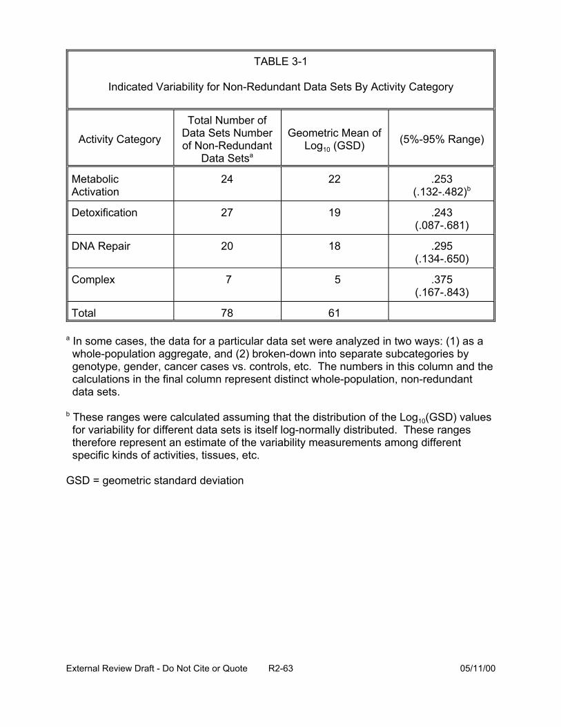
TABLE 3-1
Indicated Variability for Non-Redundant Data Sets By Activity Category
Metabolic Activation
27 19 .243 (.087-.681)
20 18 .295 (.134-.650)
7 5 .375 (.167-.843)
Total 78 61
Detoxification
DNA Repair
Complex
Activity Category
Total Number of Data Sets Number of Non-Redundant
Data Setsa
Geometric Mean of Log10 (GSD) (5%-95% Range)
24 22 .253 (.132-.482)b
a In some cases, the data for a particular data set were analyzed in two ways: (1) as a whole-population aggregate, and (2) broken-down into separate subcategories by genotype, gender, cancer cases vs. controls, etc. The numbers in this column and the calculations in the final column represent distinct whole-population, non-redundant data sets.
b These ranges were calculated assuming that the distribution of the Log10(GSD) values for variability for different data sets is itself log-normally distributed. These ranges therefore represent an estimate of the variability measurements among different specific kinds of activities, tissues, etc.
GSD = geometric standard deviation
External Review Draft - Do Not Cite or Quote R2-63 05/11/00
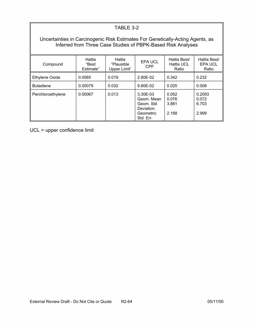
TABLE 3-2
Uncertainties in Carcinogenic Risk Estimates For Genetically-Acting Agents, as Inferred from Three Case Studies of PBPK-Based Risk Analyses
Compound Hattis “Best
Estimate”
Hattis “Plausible
Upper Limit”
EPA UCL CPF
Hattis Best/ Hattis UCL
Ratio
Hattis Best/ EPA UCL
Ratio
Ethylene Oxide 0.0065 0.019 2.80E-02 0.342 0.232
Butadiene 0.00079 0.032 9.80E-02 0.025 0.008
Perchloroethylene 0.00067 0.013 3.30E-03 Geom. Mean Geom. Std Deviation. Geometric Std. Err.
0.052 0.076 3.881
2.188
0.2093 0.072 6.703
2.999
UCL = upper confidence limit
External Review Draft - Do Not Cite or Quote R2-64 05/11/00
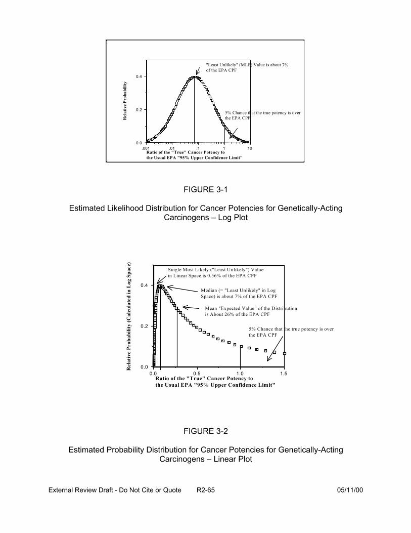
Rel
ativ
e Pr
obab
ility
101.1.01.001 0.0
0.2
0.4
Ratio of the "True" Cancer Potency to the Usual EPA "95% Upper Confidence Limit"
5% Chance that the true potency is over the EPA CPF
"Least Unlikely" (MLE) Value is about 7% of the EPA CPF
FIGURE 3-1
Estimated Likelihood Distribution for Cancer Potencies for Genetically-Acting
Rel
ativ
e Pr
obab
ility
(Cal
cula
ted
in L
og S
pace
)
0.4
0.2
0.0
Carcinogens – Log Plot
5% Chance that the true potency is over the EPA CPF
Single Most Likely ("Least Unlikely") Value in Linear Space is 0.56% of the EPA CPF
Mean "Expected Value" of the Distribution is About 26% of the EPA CPF
Median (= "Least Unlikely" in Log Space) is about 7% of the EPA CPF
0.0 0.5 1.0 1.5 Ratio of the "True" Cancer Potency to the Usual EPA "95% Upper Confidence Limit"
FIGURE 3-2
Estimated Probability Distribution for Cancer Potencies for Genetically-Acting Carcinogens – Linear Plot
External Review Draft - Do Not Cite or Quote R2-65 05/11/00
standard deviations above the median) and representing uncertainties as log-normally
distributed about a median estimate at about 0.072 times the EPA UCL, then the
geometric standard deviation of the lognormal distribution representing uncertainties is
10 [log(.0724)/1.6449] = 4.93 (Hattis and Goble, 1991; Hattis and Barlow, 1996; Hattis and
Minkowitz, 1996). Work by Crouch (1996) and by Kodell et al. (1996) showed a GSD of
10.5-11. Table 3-3 shows a scale for understanding the differences between particular
percentile of log normal distributions. For example, a GSD of 5 shows a 200-fold
difference between the 5th and 95th percentile. This is one approach to showing central
tendency and the range of variability. Another way of expressing risk in terms of both
variability and uncertainty is shown in Table 3-4. The intersection of the arithmetic
mean of the uncertainty distribution and the arithmetic mean of the variability distribution
(8.2 x 10⁻⁷) is the expected risk for an individual of unknown susceptibility.
3.2. PRESENTATION: MODELING IMPROVEMENTS - DEVELOPMENTAL DATA (B. Allen)
Developmental risk assessment has traditionally been conducted by determining
the NOAELs (no-observed-adverse effect levels) and LOAELs (lowest-observed-
adverse effect levels) in animal studies; these determinations are based on a
comparison of statistical or biological differences between groups. Uncertainty factors
are applied to the LOAELs or NOAELs for derivation of an RfD (chronic oral reference
dose) or RfC (chronic inhalation reference concentration).
Dose-response modeling as a feasible alternative to NOAEL-based approaches
is a relatively new concept in developmental toxicology. Benchmark doses (BMD) or
concentrations (BMC) can be estimated for a pre-determined response, typically one
not far from the range of observation.
External Review Draft - Do Not Cite or Quote R2-66 05/11/00
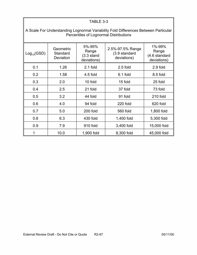
TABLE 3-3
A Scale For Understanding Lognormal Variability Fold Differences Between Particular Percentiles of Lognormal Distributions
Log10(GSD) Geometric Standard Deviation
5%-95% Range
(3.3 stand deviations)
2.5%-97.5% Range (3.9 standard deviations)
1%-99% Range
(4.6 standard deviations)
0.1
1.58 4.5 fold 6.1 fold 8.5 fold
2.0 10 fold 15 fold 25 fold
2.5 21 fold 37 fold 73 fold
3.2 44 fold 91 fold 210 fold
4.0 94 fold 220 fold 620 fold
5.0 200 fold 560 fold 1,800 fold
6.3 430 fold 1,400 fold 5,300 fold
0.9 7.9 910 fold 3,400 fold 15,000 fold
1 10.0 1,900 fold 8,300 fold 45,000 fold
0.2
0.3
0.4
0.5
0.6
0.7
0.8
1.26 2.1 fold 2.5 fold 2.9 fold
External Review Draft - Do Not Cite or Quote R2-67 05/11/00
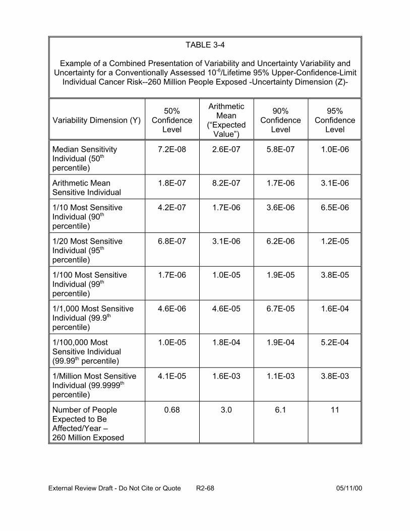
TABLE 3-4
Example of a Combined Presentation of Variability and Uncertainty Variability and Uncertainty for a Conventionally Assessed 10-6/Lifetime 95% Upper-Confidence-Limit
Individual Cancer Risk--260 Million People Exposed -Uncertainty Dimension (Z)
Variability Dimension (Y)
Median Sensitivity Individual (50th
percentile)
Arithmetic Mean Sensitive Individual
1/10 Most Sensitive Individual (90th
percentile)
1/20 Most Sensitive Individual (95th
percentile)
1/100 Most Sensitive Individual (99th
percentile)
1/1,000 Most Sensitive Individual (99.9th
percentile)
1/100,000 Most Sensitive Individual (99.99th percentile)
1/Million Most Sensitive Individual (99.9999th
percentile)
Number of People Expected to Be Affected/Year – 260 Million Exposed
50% Confidence
Level
Arithmetic Mean
(“Expected Value”)
90% Confidence
Level
95% Confidence
Level
7.2E-08 2.6E-07 5.8E-07 1.0E-06
1.8E-07 8.2E-07 1.7E-06 3.1E-06
4.2E-07 1.7E-06 3.6E-06 6.5E-06
6.8E-07 3.1E-06 6.2E-06 1.2E-05
1.7E-06 1.0E-05 1.9E-05 3.8E-05
4.6E-06 4.6E-05 6.7E-05 1.6E-04
1.0E-05 1.8E-04 1.9E-04 5.2E-04
4.1E-05 1.6E-03 1.1E-03 3.8E-03
0.68 3.0 6.1 11
External Review Draft - Do Not Cite or Quote R2-68 05/11/00
Uncertainty factors are still applied, in this case to the BMD or BMC, to derive a
regulatory limit such as an RfD or RfC.
A clear understanding of the mechanism of action is not a prerequisite for the
BMD approach. However, there are several features unique to developmental toxicity
data that must be considered in any dose-response modeling. While the dam is
considered the experimental unit, as she receives the treatment, it is the risk to the
embryo or fetus that is desired. Moreover, there may be a mixture of continuous and
quantal endpoints within and among fetuses that are measured in a developmental
study. Response may depend on a number of covariates other than dose, such as the
size of the litter. Intralitter correlation is very likely (although its magnitude is not known
with certainty and may vary depending on the endpoint(s) and mechanism of action of
the chemical insult).
Quantal endpoints (i.e., those responses for which one counts the presence or
absence of the effect) include resorption, death, malformation, or anomaly. Such
endpoints have been modeled as follows.
First, to account for intralitter correlation, one can assume that each litter has an
independent underlying probability that a fetus will be affected (for any endpoint). There
is a mean probability of response depending on dose (and litter size); the litter-specific
probabilities of response vary around the mean according to a beta distribution. Figure
3-3 shows the variety of shapes (for the probability density function) that can be
obtained with a beta distribution.
Second, one assumes that within litters, fetuses respond independently
according to a binomial model. Overall, a beta-binomial model is obtained. Responses
External Review Draft - Do Not Cite or Quote R2-69 05/11/00
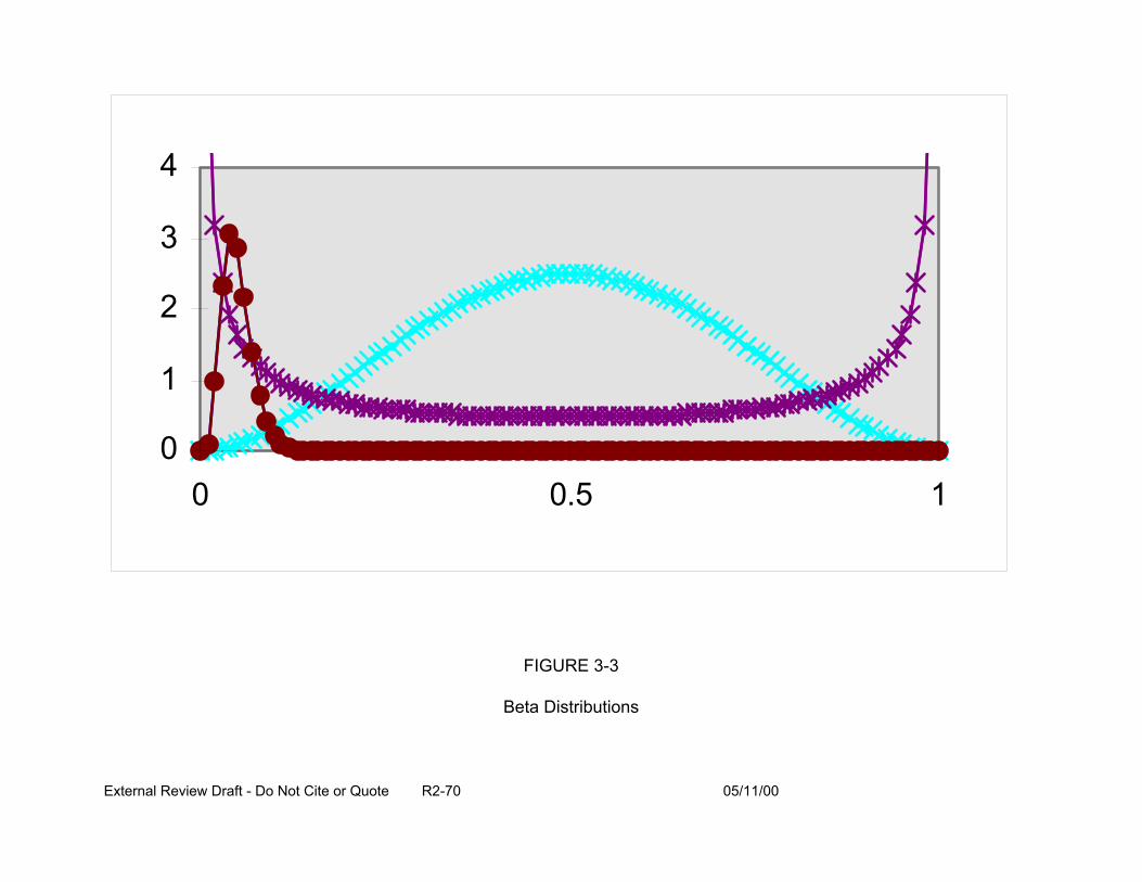
4
3
2
1
0 0 0.5
FIGURE 3-3
Beta Distributions
External Review Draft - Do Not Cite or Quote R2-70 05/11/00
1
are correlated because fetuses in the same litter (with the same underlying probability of
response) respond more similarly to one another than they do to other fetuses from
other litters.
The work of Allen et al. (1994) suggests a log-logistic model, shown below in
Equation 3-1, works well for quantal endpoints in developmental studies,
P(d,s) = a + r1s + (1 - a - r1s)/[1 + exp{B + r2s -g*log(d-d0)}] (3-1)
where d is dose, s is litter size, and d0 is the threshold dose parameter. The threshold
dose parameter as well as the parameters a, r1, r2, B, and g are estimated by the
maximum likelihood method. The log logistic model represents the relationship between
dose (and litter size) and the mean of the beta distribution of probabilities of response
discussed above.
A large-scale study of the log-logistic model (among several others) was reported
by Allen et al. (1994). The log-logistic model was compared to litter-based estimates
(estimating the probability of one or more affected fetuses within any given litter),
generic models of fetal effect probabilities (using the overall proportion of affected
fetuses without regard to grouping within litter), and two other fetal-based models
specific to developmental toxicity (the so-called Rai and Van Ryzin and NCTR models).
It was found that the log-logistic model can describe the results from a wide variety of
actual, observed developmental toxicity studies. Moreover, the comparison of the log-
logistic model to the Rai and Van Ryzin and NCTR models revealed that the log-logistic
model was more flexible in dealing with litter size effects on probability of response. In
the majority of cases studied by Allen et al. (1994), litter size was an important
explanatory variable. BMD levels were determined that, on average, afforded the same
External Review Draft - Do Not Cite or Quote R2-71 05/11/00
degree of protection as the NOAEL-based approach. When based on the log-logistic
model predictions, a 95% lower bound on the dose associated with 5% additional risk
provided that same level of protection.
Continuous endpoints, such as fetal weight or crown-rump length, are also
observed in developmental toxicity studies and can be modeled, individually, with dose-
response models. Two modeling approaches have been used. First, the “mean of
means” model, shown in Equation 3-2, estimates changes in litter means and provides
estimates of the dose-dependency of the mean of means. For any dose level, the litter
specific means are assumed to vary normally around the mean predicted by Equation 3-
2 (with, typically, each group allowed to have a variance independent of that in other
groups). A disadvantage to this approach is that there is no direct link to the calculation
of risk.
M(d) = a + b*dr (3-2)
where: a is the intercept, b is the slope, and d is dose.
A second approach to modeling continuous endpoints is to convert the
continuous response to a quantal response. For example, the probabilities of
abnormally-low fetal weight could be modeled using the log-logistic model (Equation
3-1). This model can estimate risk, but “normal” and “abnormal” response needs to be
explicitly defined by the toxicologist. The two models yield different answers
sometimes; it is not clear which model is preferable.
The multinomial modeling approach is a way to consider more than one endpoint
at a time and a means by which both quantal and continuous effects can be treated
together. Multinomial models are based on a sequence of biological events and attempt
External Review Draft - Do Not Cite or Quote R2-72 05/11/00
to represent the probability of the induction of one or more endpoints (e.g., fetal death),
as shown in Figure 3-4. These models are more complicated than the preceding
quantal or continuous models, but may be more biologically-based and may address the
issue of multiple endpoints. Developed by Chen and colleagues at NCTR and by Ryan
and colleagues at Harvard (Catalano et al., 1993), the main features of these models
are that:
• latent variables underlying the observation of malformations are considered,
• conditional probability models for malformations are dependent on fetal weight (individual and litter average), and
• the GEE (generalized estimation equation) approach is used for parameter estimation (rather than the maximum likelihood estimation).
Biologically-based models have also been considered in the context of
developmental toxicity risk assessment. Such models tend to be highly chemical-
specific, and their main advantages are associated with the fact that they incorporate
chemical-specific pharmacokinetics and pharmacodynamics and that they consider
mechanism of action information. The models of EPA’s NHERL Laboratories (Shuey et
al., 1994), David Gaylor and colleagues at NCTR (Gaylor and Razzaghi, 1992), and
Leroux and colleagues at the University of Washington (Leroux et al., 1996) are three
examples of biologically-based models.
The most complete model is that of Shuey et al., shown in Figure 3-5, wherein
the mechanism of induction of malformations and/or fetal weight reduction is modeled
based on inhibition of thymidine synthetase and subsequent effects on alteration in cell
cycling and dysmorphology. The model of Gaylor and Razzaghi considers the
External Review Draft - Do Not Cite or Quote R2-73 05/11/00
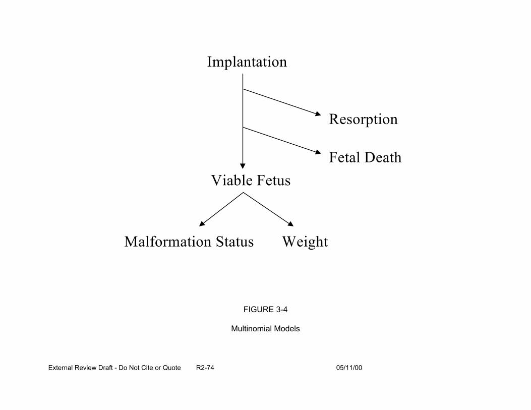
Implantation
Viable Fetus
Resorption
Fetal Death
Malformation Status Weight
FIGURE 3-4
Multinomial Models
External Review Draft - Do Not Cite or Quote R2-74 05/11/00
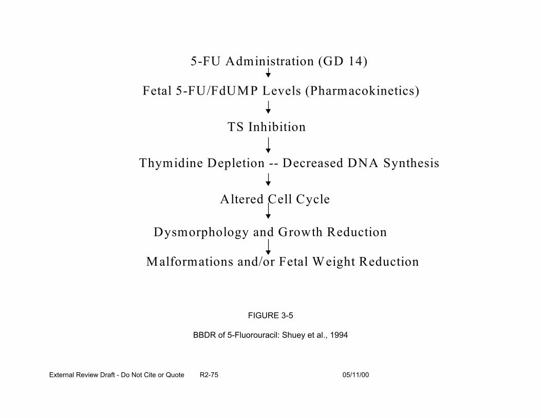
5-FU Administration (GD 14)
Fetal 5-FU/FdUMP Levels (Pharmacokinetics)
TS Inhibition
Thymidine Depletion -- Decreased DNA Synthesis
A ltered Cell Cycle
Dysmorphology and Growth Reduction
Malformations and/or Fetal Weight Reduction
FIGURE 3-5
BBDR of 5-Fluorouracil: Shuey et al., 1994
External Review Draft - Do Not Cite or Quote R2-75 05/11/00
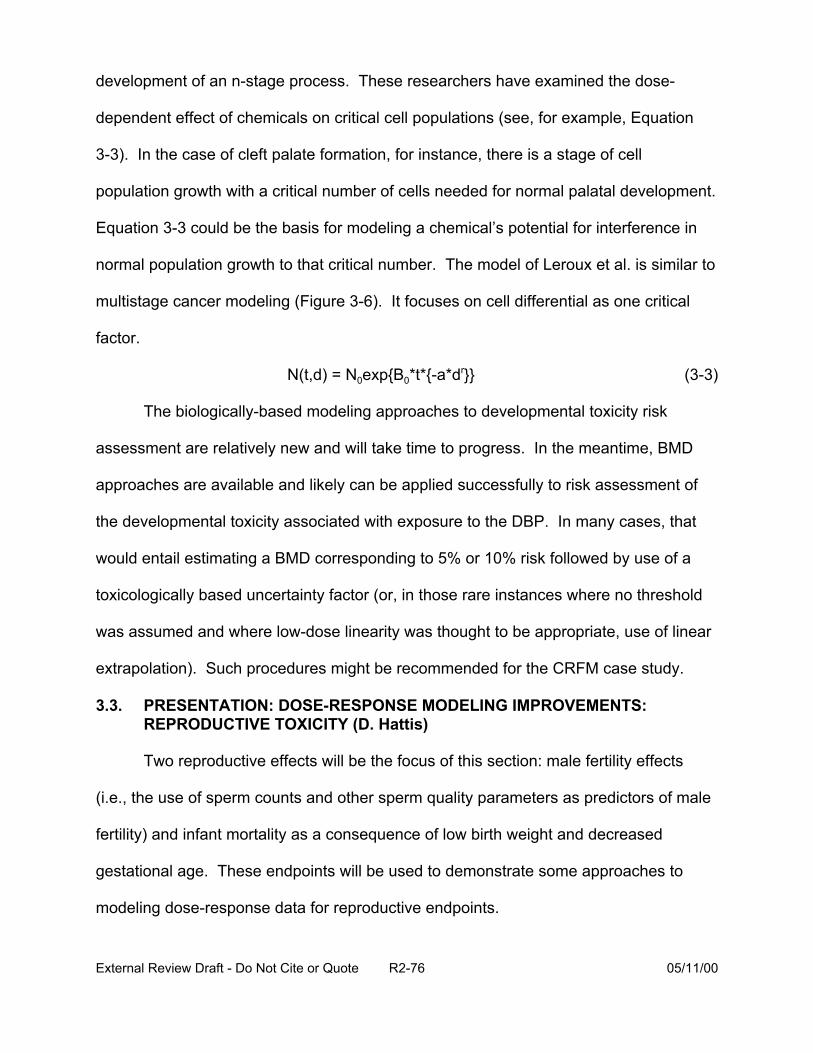
development of an n-stage process. These researchers have examined the dose-
dependent effect of chemicals on critical cell populations (see, for example, Equation
3-3). In the case of cleft palate formation, for instance, there is a stage of cell
population growth with a critical number of cells needed for normal palatal development.
Equation 3-3 could be the basis for modeling a chemical’s potential for interference in
normal population growth to that critical number. The model of Leroux et al. is similar to
multistage cancer modeling (Figure 3-6). It focuses on cell differential as one critical
factor.
N(t,d) = N0exp{B0*t*{-a*dr}} (3-3)
The biologically-based modeling approaches to developmental toxicity risk
assessment are relatively new and will take time to progress. In the meantime, BMD
approaches are available and likely can be applied successfully to risk assessment of
the developmental toxicity associated with exposure to the DBP. In many cases, that
would entail estimating a BMD corresponding to 5% or 10% risk followed by use of a
toxicologically based uncertainty factor (or, in those rare instances where no threshold
was assumed and where low-dose linearity was thought to be appropriate, use of linear
extrapolation). Such procedures might be recommended for the CRFM case study.
3.3. PRESENTATION: DOSE-RESPONSE MODELING IMPROVEMENTS: REPRODUCTIVE TOXICITY (D. Hattis)
Two reproductive effects will be the focus of this section: male fertility effects
(i.e., the use of sperm counts and other sperm quality parameters as predictors of male
fertility) and infant mortality as a consequence of low birth weight and decreased
gestational age. These endpoints will be used to demonstrate some approaches to
modeling dose-response data for reproductive endpoints.
External Review Draft - Do Not Cite or Quote R2-76 05/11/00
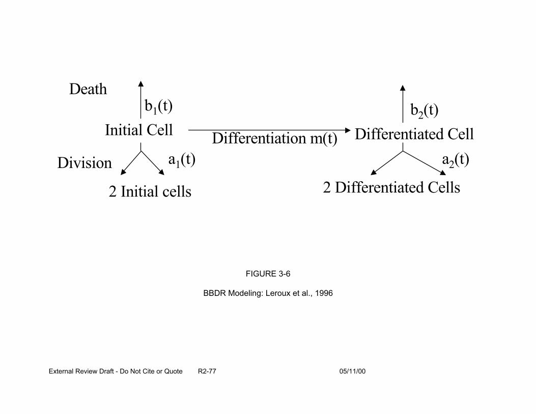
Death b1(t)
Initial Cell b2(t)
Differentiation m(t) Differentiated Cell
Division a1(t) a2(t)
2 Initial cells 2 Differentiated Cells
FIGURE 3-6
BBDR Modeling: Leroux et al., 1996
External Review Draft - Do Not Cite or Quote R2-77 05/11/00
Sperm count and other sperm quality parameters are used as predictors of male
fertility. One approach is to evaluate the incidence of infertility. For example, Meistrich
and Brown (1983) defined the increase in “% infertility” as the fraction of couples
presenting themselves for evaluation and treatment after at least a year of unprotected
intercourse. Another approach is to model the effect of sperm counts on the per-cycle
conception probability and the distribution of conception times. Data supporting this
approach include couples presenting themselves for treatment of infertility (Steinberger
and Rodrigues-Rigau, 1983); data from artificial insemination (Hattis, 1998); and data
from prospective studies of “unselected” couples (Clegg, 1999). Hattis (1998) analyzed
the data of Brasch et al. (1994), which provided the frequency of conception per cycle
for intrauterine insemination as a function of the total number of motile sperm that are
available for use. The relationship was far less than linear; that is, increasing numbers
of sperm increase the probability of conception, but not proportionately (Figure 3-7). If
80 million sperm are available, then the conception probability is a little less than double
what it would be with only 3-8 million sperm. Clegg (1999) found that the most
important parameters are the total number of sperm and the percentage of strictly
normal sperm; each parameter has high-dose saturating behavior. That is, there is a
point at which increases in sperm count are not linearly-related to increased fertility.
Over many orders of magnitude, there is a strong relationship between infant
mortality and birth weight (Figure 3-8). Birth weight is likely a marker for incomplete
development. Hattis and coworkers (Ballew and Hattis, 1989; Rees and Hattis, 1994;
Hattis, 1998) conducted an analysis of the implications of reduced fetal weights in
relation to glycol ether exposures in animals. Fetal weight was used as a predictor for
External Review Draft - Do Not Cite or Quote R2-78 05/11/00
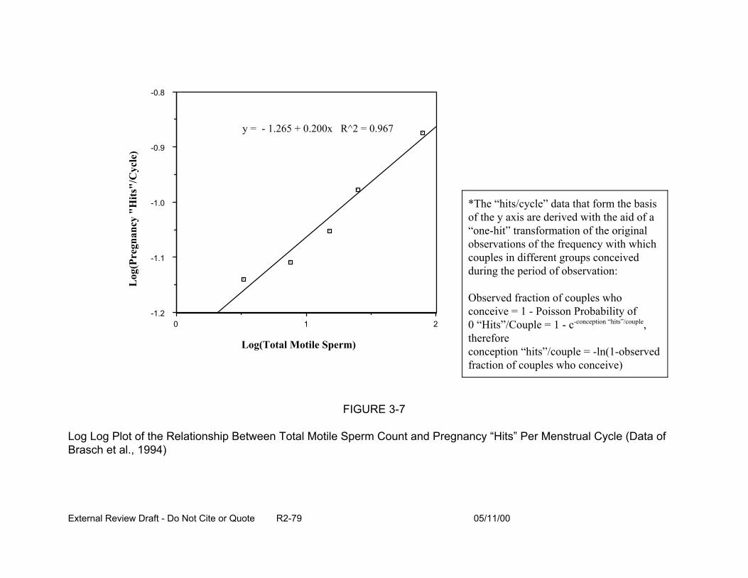
Log
(Pre
gnan
cy "
Hits
"/C
ycle
)
-0.8
-0.9
-1.0
-1.1
-1.2
y = R^2 = 0.967 - 1.265 + 0.200x
Log(Total Motile Sperm)
FIGURE 3-7
*The “hits/cycle” data that form the basisof the y axis are derived with the aid of a“one-hit” transformation of the originalobservations of the frequency with whichcouples in different groups conceivedduring the period of observation:
Observed fraction of couples whoconceive = 1 - Poisson Probability of0 “Hits”/Couple = 1 - c-conception “hits”/couple,thereforeconception “hits”/couple = -ln(1-observedfraction of couples who conceive)
0 1 2
Log Log Plot of the Relationship Between Total Motile Sperm Count and Pregnancy “Hits” Per Menstrual Cycle (Data of Brasch et al., 1994)
External Review Draft - Do Not Cite or Quote R2-79 05/11/00
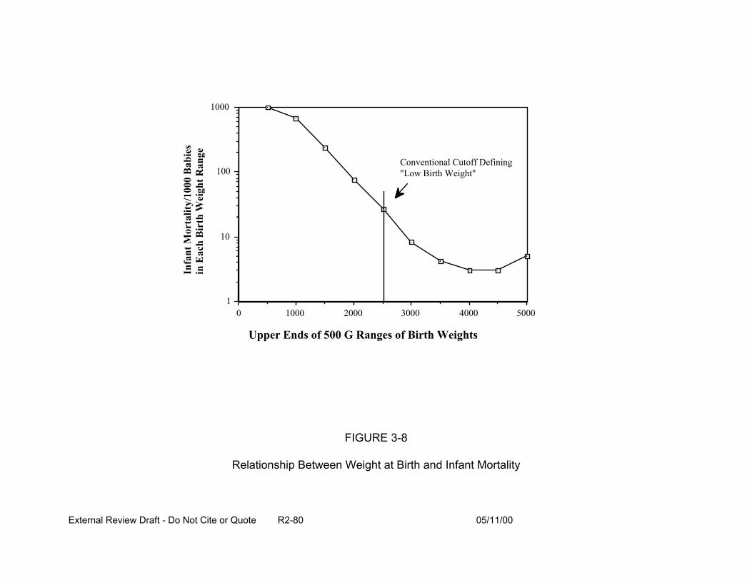
Infa
nt M
orta
lity/
1000
Bab
ies
in E
ach
Bir
th W
eigh
t Ran
ge
1000
100
10
1
Conventional Cutoff Defining "Low Birth Weight"
0 1000 2000 3000 4000 5000
Upper Ends of 500 G Ranges of Birth Weights
FIGURE 3-8
Relationship Between Weight at Birth and Infant Mortality
External Review Draft - Do Not Cite or Quote R2-80 05/11/00

fetal mortality (see Figure 3-9). Recent tests of the predictive accuracy of the
relationship between birth weight and infant mortality have included the effect of
smoking on birth weight and the incidence of premature births (<37 weeks of gestation).
The effects of smoking on birth weights and prematurity predict the magnitude of the
effect of various amounts of smoking on infant mortality. Advantages to using birth
weight are that it:
• is a continuous variable and statistically powerful,
• is an important predictor of responses that are not easily measured directly (e.g., infant mortality), and
• responds to modest degrees of environmental exposure.
The latter is supported by data on cigarette smoking from the 1990 Birth Cohort
Linked Birth/Infant Death Data Set (NCHS, 1996), where 6 cigarettes/day produces a
180 g reduction in birth weight (Figure 3-10), and by data on altitude (Cogswell and Yip,
1995), where 4000 feet elevation results in a 70 g reduction in birth weight (Figure
3-11). Disadvantages to using birth weight as a biomarker for potential adverse effects,
are that it:
• is affected by many “confounders”, many of which are not recorded on birth certificates and cannot be controlled, and
• is a non-specific indicator (i.e., it does not provide information on distinctive exposures).
One approach would be to use sperm count, fetal weights, or another endpoint
as a biomarker for potential human effects. After dose-response modeling, the results
would be extrapolated to humans (e.g., using BW3/4 power). The significance of these
markers would be interpreted from human information. This approach was applied to
the animal fetal weight data of Smith et al. (1988) after exposure to trichloroacetonitrile
External Review Draft - Do Not Cite or Quote R2-81 05/11/00

Infa
nt D
eath
s Per
100
0 B
abie
s of A
ll B
irth
Wei
ght i
n th
e T
otal
Pop
ulat
ion
2
1
0
Total Infant Deaths Per 1000 Births
9.07 9.51
Mort/1000 Births--Orig Pop.
Mort/1000 Births--1% Weight Red .44 Expected increase for 1% reduction in birth weights
500 1000 1500 2000 2500 3000 3500 4000 4500 5000
Upper Ends of 500 G Ranges of Birth Weights
FIGURE 3-9
Expected Effect of a 1% Reduction in Birth Weights on the Distribution of Overall Infant Deaths Per 1000 Babies Born in the Total Population
External Review Draft - Do Not Cite or Quote R2-82 05/11/00
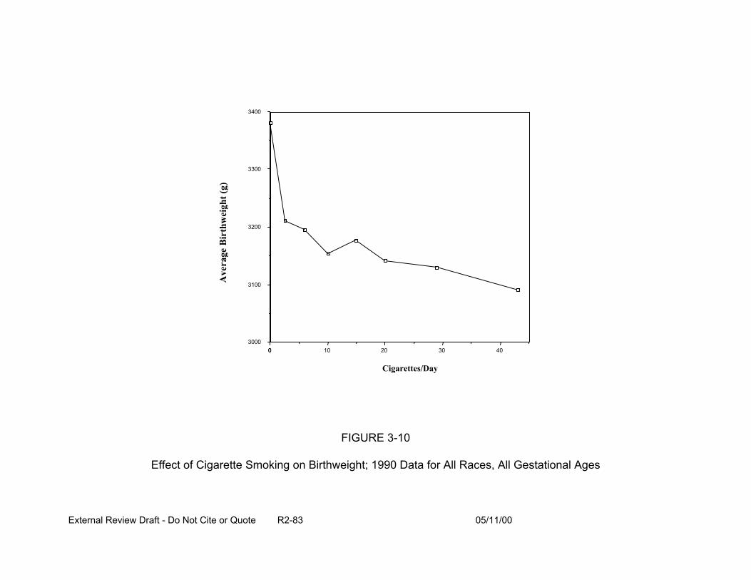
0
3400
3300
3200
3100
3000 0 10 20 30 40
Cigarettes/Day
FIGURE 3-10
Effect of Cigarette Smoking on Birthweight; 1990 Data for All Races, All Gestational Ages
Ave
rage
Bir
thw
eigh
t (g)
External Review Draft - Do Not Cite or Quote R2-83 05/11/00
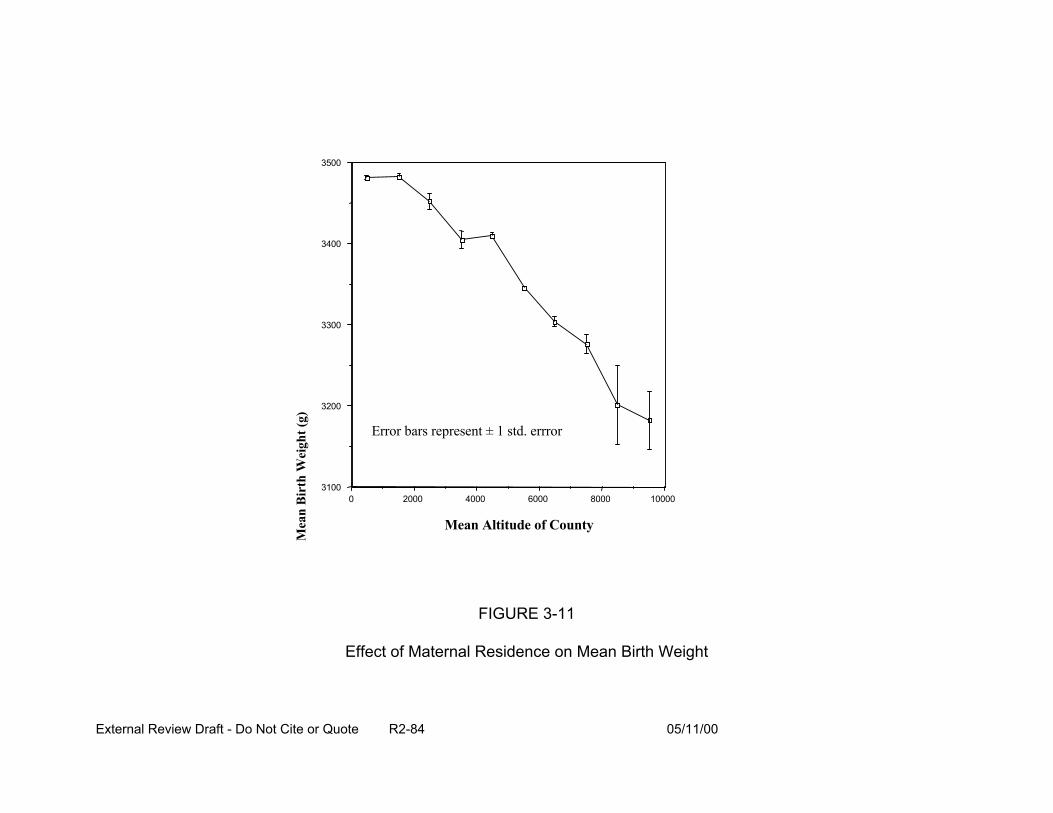
Mea
n B
irth
Wei
ght (
g)
3500
3400
3300
3200
31000 2000 4000 6000 8000 10000
Error bars represent ± 1 std. errror
Mean Altitude of County
FIGURE 3-11
Effect of Maternal Residence on Mean Birth Weight
External Review Draft - Do Not Cite or Quote R2-84 05/11/00
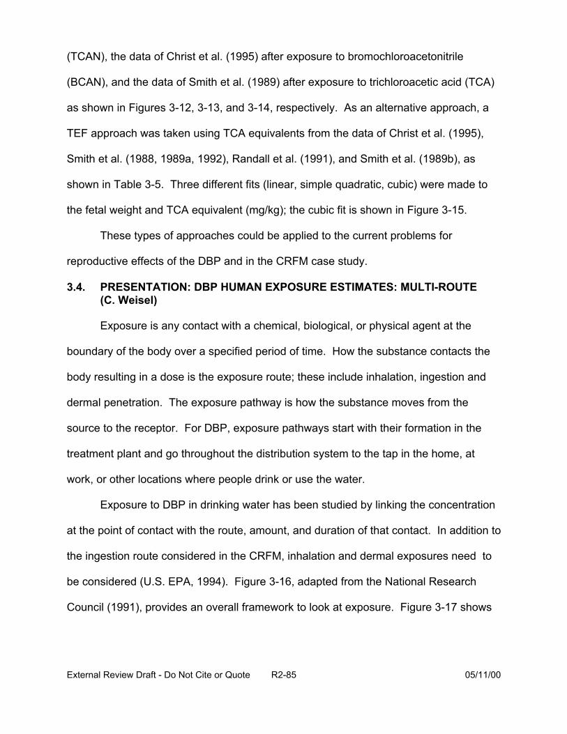
(TCAN), the data of Christ et al. (1995) after exposure to bromochloroacetonitrile
(BCAN), and the data of Smith et al. (1989) after exposure to trichloroacetic acid (TCA)
as shown in Figures 3-12, 3-13, and 3-14, respectively. As an alternative approach, a
TEF approach was taken using TCA equivalents from the data of Christ et al. (1995),
Smith et al. (1988, 1989a, 1992), Randall et al. (1991), and Smith et al. (1989b), as
shown in Table 3-5. Three different fits (linear, simple quadratic, cubic) were made to
the fetal weight and TCA equivalent (mg/kg); the cubic fit is shown in Figure 3-15.
These types of approaches could be applied to the current problems for
reproductive effects of the DBP and in the CRFM case study.
3.4. PRESENTATION: DBP HUMAN EXPOSURE ESTIMATES: MULTI-ROUTE (C. Weisel)
Exposure is any contact with a chemical, biological, or physical agent at the
boundary of the body over a specified period of time. How the substance contacts the
body resulting in a dose is the exposure route; these include inhalation, ingestion and
dermal penetration. The exposure pathway is how the substance moves from the
source to the receptor. For DBP, exposure pathways start with their formation in the
treatment plant and go throughout the distribution system to the tap in the home, at
work, or other locations where people drink or use the water.
Exposure to DBP in drinking water has been studied by linking the concentration
at the point of contact with the route, amount, and duration of that contact. In addition to
the ingestion route considered in the CRFM, inhalation and dermal exposures need to
be considered (U.S. EPA, 1994). Figure 3-16, adapted from the National Research
Council (1991), provides an overall framework to look at exposure. Figure 3-17 shows
External Review Draft - Do Not Cite or Quote R2-85 05/11/00
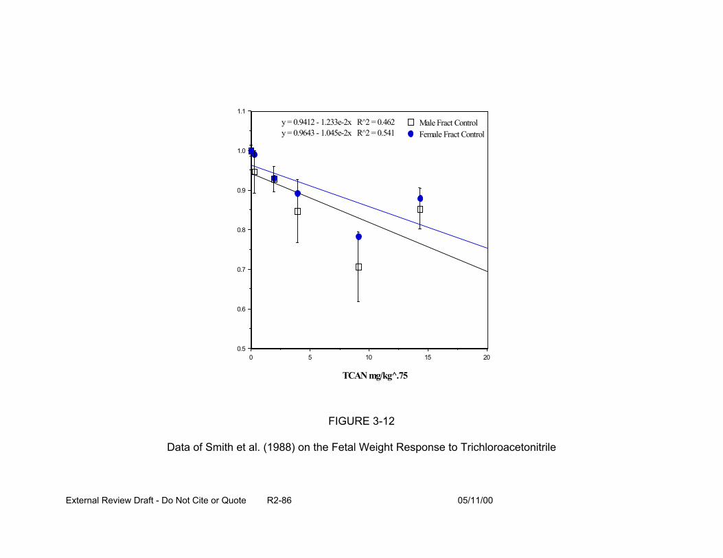
1.1
1.0
0.9
0.8
0.7
0.6
0.5 0 5
Male Fract Control Female Fract Control
y = 0.9412 - 1.233e-2x R^2 = 0.462 y = 0.9643 - 1.045e-2x R^2 = 0.541
10 15 20
TCAN mg/kg .̂75
FIGURE 3-12
Data of Smith et al. (1988) on the Fetal Weight Response to Trichloroacetonitrile
External Review Draft - Do Not Cite or Quote R2-86 05/11/00
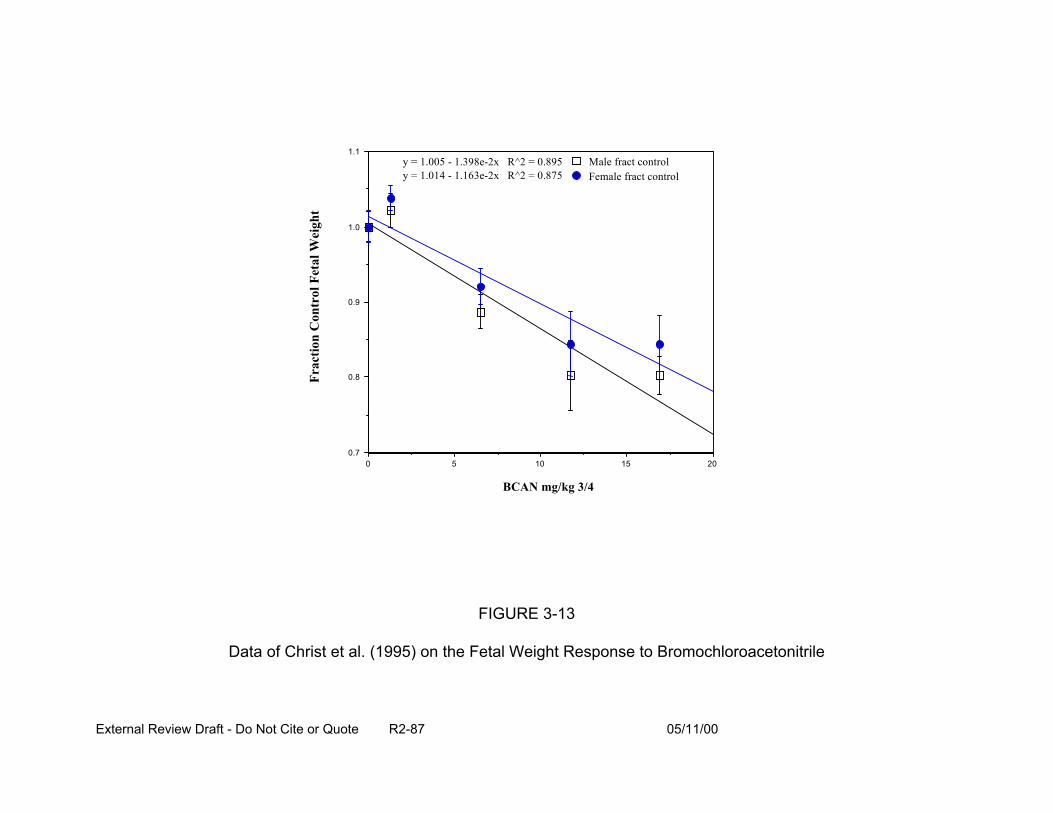
1.1
Frac
tion
Con
trol
Fet
al W
eigh
t
1.0
0.9
0.8
0.7 0 5
Male fract control Female fract control
y = 1.005 - 1.398e-2x R^2 = 0.895 y = 1.014 - 1.163e-2x R^2 = 0.875
10
BCAN mg/kg 3/4
15 20
FIGURE 3-13
Data of Christ et al. (1995) on the Fetal Weight Response to Bromochloroacetonitrile
External Review Draft - Do Not Cite or Quote R2-87 05/11/00
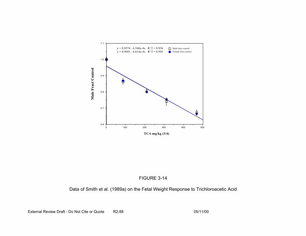
Mal
e Fr
act C
ontr
ol
1.1
1.0
0.9
0.8
0.7
0.6
Male fract control Female fract control
y = 0.9574 - 6.548e-4x ^2 = 0.936 y = 0.9601 - 6.614e-4x ^2 = 0.945
RR
0 100 200 300 400 500
TCA mg/kg (3/4)
FIGURE 3-14
Data of Smith et al. (1989a) on the Fetal Weight Response to Trichloroacetic Acid
External Review Draft - Do Not Cite or Quote R2-88 05/11/00
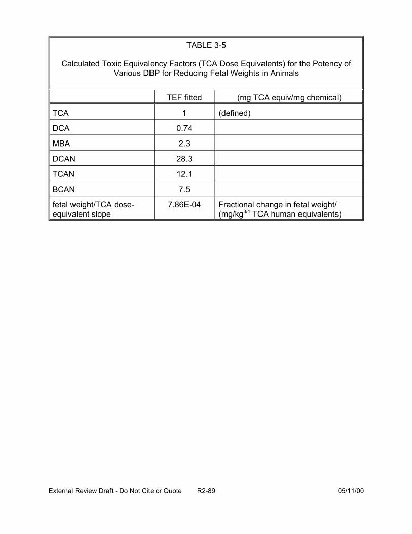
TABLE 3-5
Calculated Toxic Equivalency Factors (TCA Dose Equivalents) for the Potency of Various DBP for Reducing Fetal Weights in Animals
TEF fitted (mg TCA equiv/mg chemical)
TCA 1
DCA 0.74
MBA 2.3
DCAN 28.3
TCAN 12.1
(defined)
BCAN 7.5
fetal weight/TCA dose-equivalent slope
7.86E-04 Fractional change in fetal weight/ (mg/kg3/4 TCA human equivalents)
External Review Draft - Do Not Cite or Quote R2-89 05/11/00

1.1
1.0
0.9
0.8
0.7
0.6 0 100 200 300 400 500
y = 1.0069 - 1.1137e-3x + 8.6176e-7x^2 ^2 = 0.983 R
TCA equiv mg/kg
FIGURE 3-15
Results of Regression Analysis of the Fraction of Control Fetal Weight Response in Grouped Categories of TCA Equivalents
Frac
t Con
trol
Fet
al W
eigh
t
External Review Draft - Do Not Cite or Quote R2-90 05/11/00
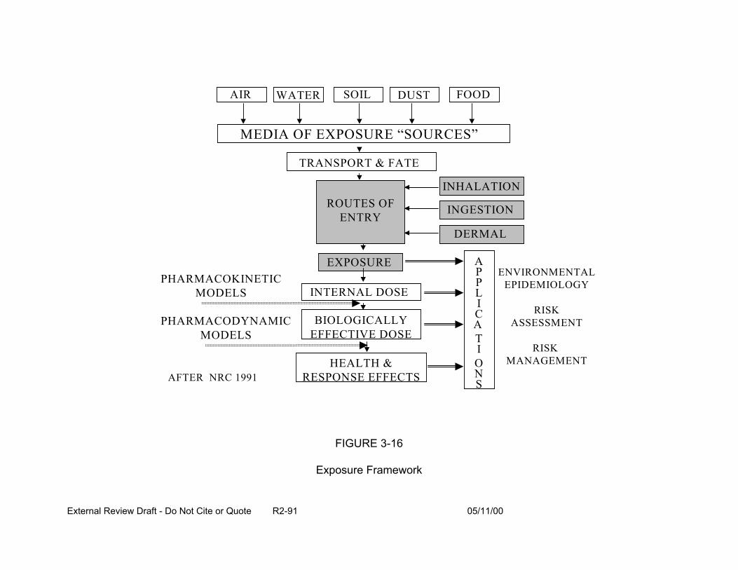
AIR WATER SOIL DUST FOOD
MEDIA OF EXPOSURE “SOURCES”
TRANSPORT & FATE
INHALATION
INGESTIONROUTES OF ENTRY
EXPOSURE
DERMAL
A P ENVIRONMENTALPHARMACOKINETIC
MODELS
PHARMACODYNAMIC MODELS
AFTER NRC 1991
INTERNAL DOSE
BIOLOGICALLY EFFECTIVE DOSE
P L I C A
EPIDEMIOLOGY
RISK ASSESSMENT
RISK MANAGEMENT
T I
HEALTH & O RESPONSE EFFECTS N
S
FIGURE 3-16
Exposure Framework
External Review Draft - Do Not Cite or Quote R2-91 05/11/00
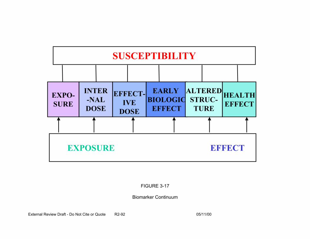
EXPO-SURE
INTER -NAL DOSE
EFFECT-IVE
DOSE
EARLY BIOLOGIC
EFFECT
ALTERED STRUC-TURE
HEALTH EFFECT
SUSCEPTIBILITY
EXPOSURE EFFECT
FIGURE 3-17
Biomarker Continuum
External Review Draft - Do Not Cite or Quote R2-92 05/11/00
the continuum of biomarkers from exposure to internal dose of the agent and, effective
dose at the target tissue, through induction of an early biologic effect (related to
sensitivity and susceptibility of individuals and subpopulations), through alteration of
structure (such as RNA and DNA) and adverse health effect(s). Approaches to
evaluating DBP include conducting:
• individual exposure assessment,
• ecological epidemiological study, and /or,
• case control or cohort studies.
Each of these approaches uses a variety of tools, such as:
• questionnaires,
• multimedia measurements (e.g., in air, water)
• biomarker measurements,
• modeling (for population exposure assessments), and
• historic reconstruction (to understand what happened in the past).
Studies of DBP in water indicate multiple exposure routes; looking only at
ingestion of DBP is not sufficient for estimating exposure. Shower stall and indoor air
concentrations are elevated with respect to volatile DBP after showers and other water
uses. As shown by measurement of biomarkers in studies of aqueous solutions in
animals and in in vitro studies, some DBP cross the skin. Blood, breath, and urine DBP
levels are elevated after showering, bathing, and swimming; as the concentration of
volatile DBP increase, so do the levels of the biomarkers.
The shower studies of Weisel et al. (1990; Jo et al., 1990a, 1990b) evaluated the
influence of inhalation and dermal exposure to DBP, specifically chloroform,
External Review Draft - Do Not Cite or Quote R2-93 05/11/00
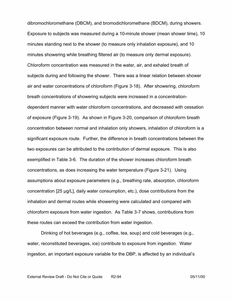
dibromochloromethane (DBCM), and bromodichloromethane (BDCM), during showers.
Exposure to subjects was measured during a 10-minute shower (mean shower time), 10
minutes standing next to the shower (to measure only inhalation exposure), and 10
minutes showering while breathing filtered air (to measure only dermal exposure).
Chloroform concentration was measured in the water, air, and exhaled breath of
subjects during and following the shower. There was a linear relation between shower
air and water concentrations of chloroform (Figure 3-18). After showering, chloroform
breath concentrations of showering subjects were increased in a concentration-
dependent manner with water chloroform concentrations, and decreased with cessation
of exposure (Figure 3-19). As shown in Figure 3-20, comparison of chloroform breath
concentration between normal and inhalation only showers, inhalation of chloroform is a
significant exposure route. Further, the difference in breath concentrations between the
two exposures can be attributed to the contribution of dermal exposure. This is also
exemplified in Table 3-6. The duration of the shower increases chloroform breath
concentrations, as does increasing the water temperature (Figure 3-21). Using
assumptions about exposure parameters (e.g., breathing rate, absorption, chloroform
concentration [25 :g/L], daily water consumption, etc.), dose contributions from the
inhalation and dermal routes while showering were calculated and compared with
chloroform exposure from water ingestion. As Table 3-7 shows, contributions from
these routes can exceed the contribution from water ingestion.
Drinking of hot beverages (e.g., coffee, tea, soup) and cold beverages (e.g.,
water, reconstituted beverages, ice) contribute to exposure from ingestion. Water
ingestion, an important exposure variable for the DBP, is affected by an individual’s
External Review Draft - Do Not Cite or Quote R2-94 05/11/00
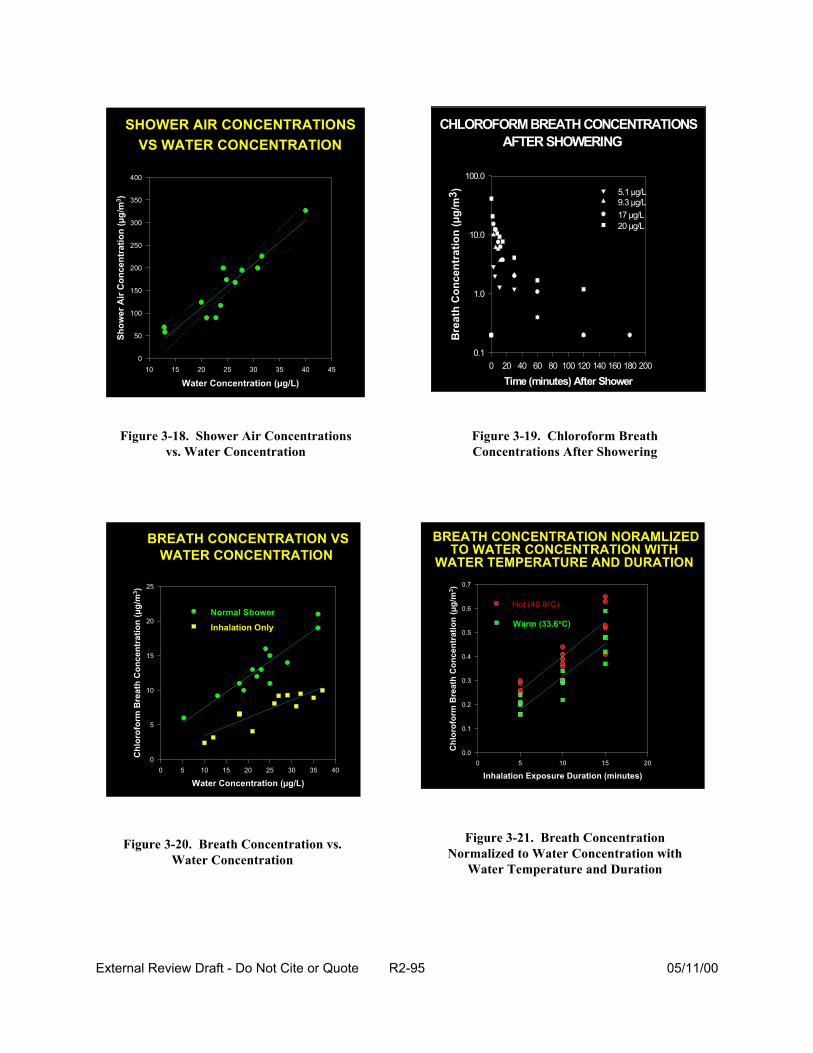
SHOWER AIR CONCENTRATIONS
Water Concentration (µg/L) 10 15 20 25 30 35 40 45
Show
er A
ir C
once
ntra
tion
(µg/
m3 )
0
50
100
150
200
250
300
350
400
VS WATER CONCENTRATION CHLOROFORM BREATH CONCENTRATIONS
Time (minutes) After Shower 0 20 40 60 80 100 120 140 160 180 200
Bre
ath
Con
cent
ratio
n (µ
g/m
3 )
0.1
1.0
10.0
100.0
17 µg/L 20 µg/L
9.3 µg/L 5.1 µg/L
AFTER SHOWERING
Figure 3-18. Shower Air Concentrations Figure 3-19. Chloroform Breath vs. Water Concentration Concentrations After Showering
BREATH CONCENTRATION VS
Water Concentration (µg/L) 0 5 10 15 20 25 30 35 40
Chl
orof
orm
Bre
ath
Con
cent
ratio
n (µ
g/m
3 )
0
5
10
15
20
25
WATER CONCENTRATION
Normal Shower
Inhalation Only
BREATH CONCENTRATION NORAMLIZED
Inhalation Exposure Duration (minutes) 0 5 10 15 20
Chl
orof
orm
Bre
ath
Con
cent
ratio
n (µ
g/m
3 )
0.0
0.1
0.2
0.3
0.4
0.5
0.6
0.7
TO WATER CONCENTRATION WITH WATER TEMPERATURE AND DURATION
Hot (40.8oC)
Warm (33.6oC)
Figure 3-21. Breath ConcentrationFigure 3-20. Breath Concentration vs. Normalized to Water Concentration withWater Concentration
Water Temperature and Duration
External Review Draft - Do Not Cite or Quote R2-95 05/11/00
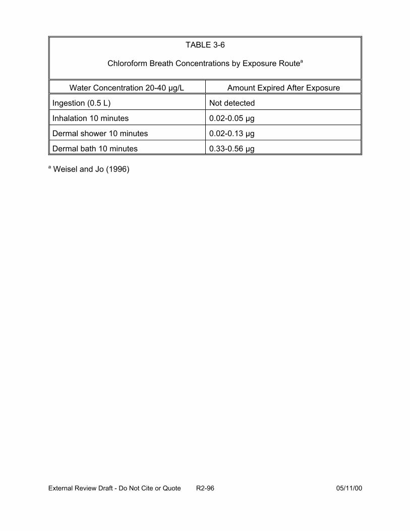
TABLE 3-6
Chloroform Breath Concentrations by Exposure Routea
Ingestion (0.5 L)
Inhalation 10 minutes
Dermal shower 10 minutes
Dermal bath 10 minutes
a Weisel and Jo (1996)
Water Concentration 20-40 µg/L Amount Expired After Exposure
Not detected
0.02-0.05 µg
0.02-0.13 µg
0.33-0.56 µg
External Review Draft - Do Not Cite or Quote R2-96 05/11/00
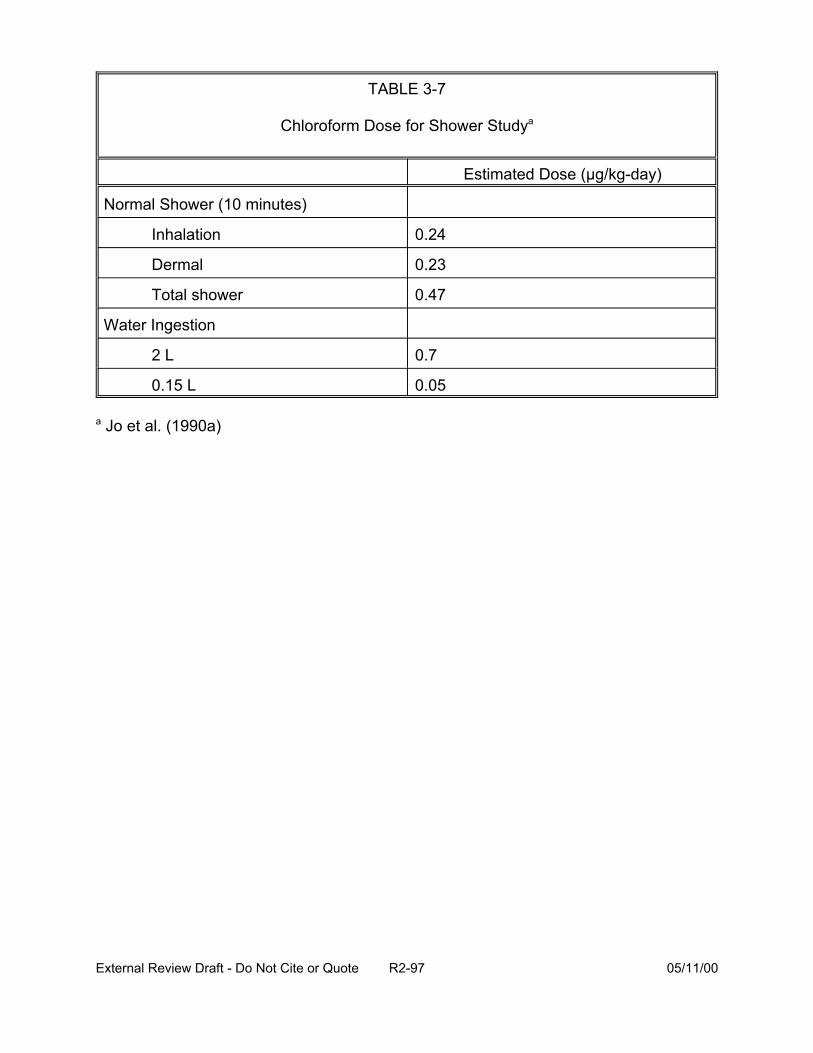
TABLE 3-7
Chloroform Dose for Shower Studya
Estimated Dose (µg/kg-day)
Normal Shower (10 minutes)
Inhalation 0.24
Dermal 0.23
Total shower 0.47
Water Ingestion
2 L 0.7
0.15 L 0.05
a Jo et al. (1990a)
External Review Draft - Do Not Cite or Quote R2-97 05/11/00
habits (such as exercise), season/climate, and location/region. Median tap water
ingestion is approximately 1.61 L/day (0.77-2.6 L/day is the range for the 10th- 90th
percentiles). The temperature of the water affects the concentrations of some
chemicals and may decompose other chemicals. For example, boiling of the water
increases the concentration of nonvolatile chemicals. In contrast, heating of water
volatilizes some chemicals (such as THM), decreasing their concentration in the water,
but increasing their concentration in the air. These volatile species are released into the
air based on Henry’s Law and can be measured within shower stalls, over sinks, and in
indoor air. Aerosol formation of non-volatile species occurs during spray of the water;
aerosol spray undergoes size redistribution within the home. In addition to showering,
vapors and aerosols are generated during humidifier use (likely a very important
source), washing, bathing and other activities in the home contributing to levels of
chemicals in indoor air. For showering/bathing, U.S. EPA (1997) uses defaults of 10
minutes (the median is closer to 7 minutes), 1 shower/day (although 5% of the
population shower more than once per day), 350 days/year. The 50th, 75th, and 90th
percentiles for shower duration are 7, 9, and 12 minutes/day, respectively.
Inhalation exposure through distribution of vapors and aerosols within a home
can be modeled. Air exchange processes are described to establish spatial and
temporal changes in air concentrations. Use of water filters and hot water heaters are
evaluated to determine whether a constant or variable water concentration is to be used
for modeling. Breathing rate is a variable considered in estimating dose (Wilkes et al.,
1996; Wilkes, 1999).
External Review Draft - Do Not Cite or Quote R2-98 05/11/00
Direct dermal contact with DBP in water occurs during showering and bathing
and also with washing and swimming. For small children (e.g., 3-7 years old), playing in
wading pools may be a significant source of contact with these chemicals during the
summer months. Two approaches have generally been used for modeling dermal
exposures: steady state transference using permeability coefficients across the stratum
corneum, and membrane flux, which considers skin structure, flux across the skin by
skin type, and permeability coefficients (Roy et al., 1996; Bunge and McDougal, 1999).
Estimates of exposure concentrations from air or water are overlaid with
“allowable” or reasonable scenarios and activity patterns to generate exposure
distributions for the population. Activity patterns and other variables for the specific
region are investigated so that water use patterns and other characteristics of the
population can be established. Often, simulation routines (e.g., Monte Carlo
techniques) are used to describe distributions of air and water uses, frequency, and
duration. Consideration of age and years in residences (transient population groups),
and changes in water concentrations over time are considered when examining chronic
exposures. For acute exposures, the time of year for peak concentrations or other
events are factored into predicting acute health outcomes (e.g., birth-related effects). A
summary of the relative importance of various media in contributing to population dose
is shown in Table 3-8 for chloroform and a non-volatile species (i.e., chromium).
Approaches to estimating exposure in epidemiological studies have focused on
areas using chlorinated water based on chlorine use at the treatment plant over time.
Measured or predicted concentrations of THM at the treatment plant are combined with
External Review Draft - Do Not Cite or Quote R2-99 05/11/00
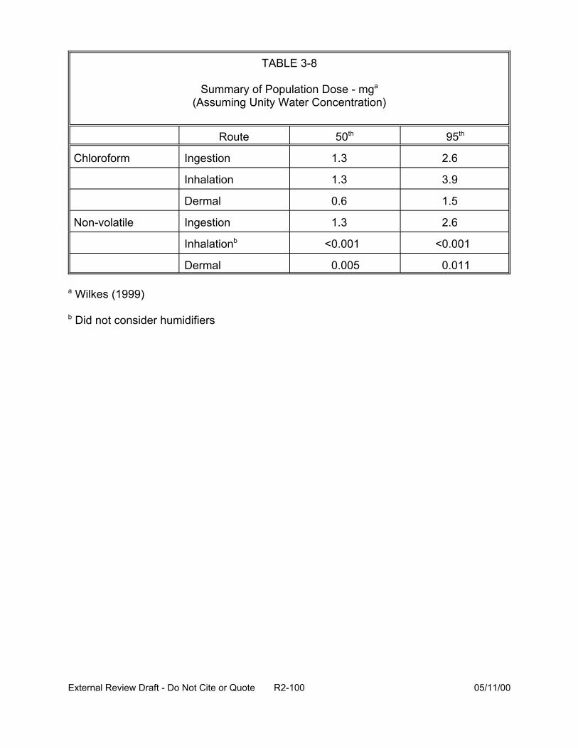
TABLE 3-8
Summary of Population Dose - mga
(Assuming Unity Water Concentration)
Route 50th 95th
1.3 2.6
Inhalation 1.3 3.9
Dermal 0.6 1.5
Non-volatile Ingestion 1.3 2.6
Inhalationb <0.001 <0.001
Dermal 0.005 0.011
Chloroform
a Wilkes (1999)
Ingestion
b Did not consider humidifiers
External Review Draft - Do Not Cite or Quote R2-100 05/11/00
responses from residents to questionnaires. Questionnaires attempt to obtain
information on:
• source of water and use of filtration systems,
• types and amounts of water used for cooking, bottled water use, and hot and cold water use,
• frequency, duration, and water temperature for showering and bathing,
• other water uses, such as humidifiers, washing, dishwasher, and washing machines,
• target populations, i.e., their location, activities, seasonality, children, pregnant and lactating women, time spent away from home (e.g., at work), and
• potential confounders, such as swimming and non-residential use.
Because water concentrations vary spatially and temporally, there are continued
reactions with chlorine residuals and microbial degradation within the distribution
system. THM may not be the biologically-active agent. Estimating exposure using only
the ingestion route may not be accurate. Therefore, exposure may be misclassified in
epidemiological studies due to these factors.
The Total Exposure Assessment Methodology (TEAM) study (Wallace et al.,
1985, 1986, 1987) and more recent studies by Weisel et al. (1999b) are examples of
population-based studies. These studies measured THM in indoor air. Median indoor
chloroform levels were four times higher than outdoor levels in New Jersey, suggesting
to the authors that water use was the source of chloroform (Wallace et al., 1987). THM
breath concentrations, unlike some other volatile organic compounds, were related to
water concentration, not indoor air concentration. More recent THM breath
concentrations in New Jersey (Weisel et al., 1999b) showed lower levels than those
External Review Draft - Do Not Cite or Quote R2-101 05/11/00
found by TEAM. Although associations were still found, the authors attributed the lower
breath levels to lower water concentrations of these chemicals. Post-shower breath
concentrations documented the strong association for THM with water concentration
(Tables 3-9, 3-10, and 3-11). The concentration and ingestion of trichloroacetic acid
(TCAA) and dichloroacetic acid (DCAA) in water were compared with their urinary
excretion in a population of 48 subjects and a subset of the population comprised of 25
subjects who ingested water only at home where the drinking water was analyzed
(Weisel et al., 1999b). An association between the amount of TCAA ingested
calculated as the product of water concentration and amount of water ingested was
identified across all subjects. That association was stronger in the subset of individuals
who only ingested water at home, when misclassification was reduced. These
associations suggest a dose-response relationship for urinary TCAA as biomarker. In
addition, while the excretion rate of TCAA was associated with ingestion for those
subjects who drank water only at home (Figure 3-22), it was not related to water
concentration of TCAA (Figure 3-23), indicating that water concentration is not a good
measure of exposure to TCAA since it does not account for the variability in the amount
of water ingested by the population. No associations were found between DCAA water
concentration and DCAA excretion rate or for water ingestion and excretion of DCAA.
This suggests that urinary DCAA is not good biomarker of exposure to DCAA, with its
rapid metabolism rate being the likely cause.
In conclusion, both breath and urinary biomarkers can be developed for DBP and
can be used in epidemiological studies; however, knowledge of residence time is
External Review Draft - Do Not Cite or Quote R2-102 05/11/00
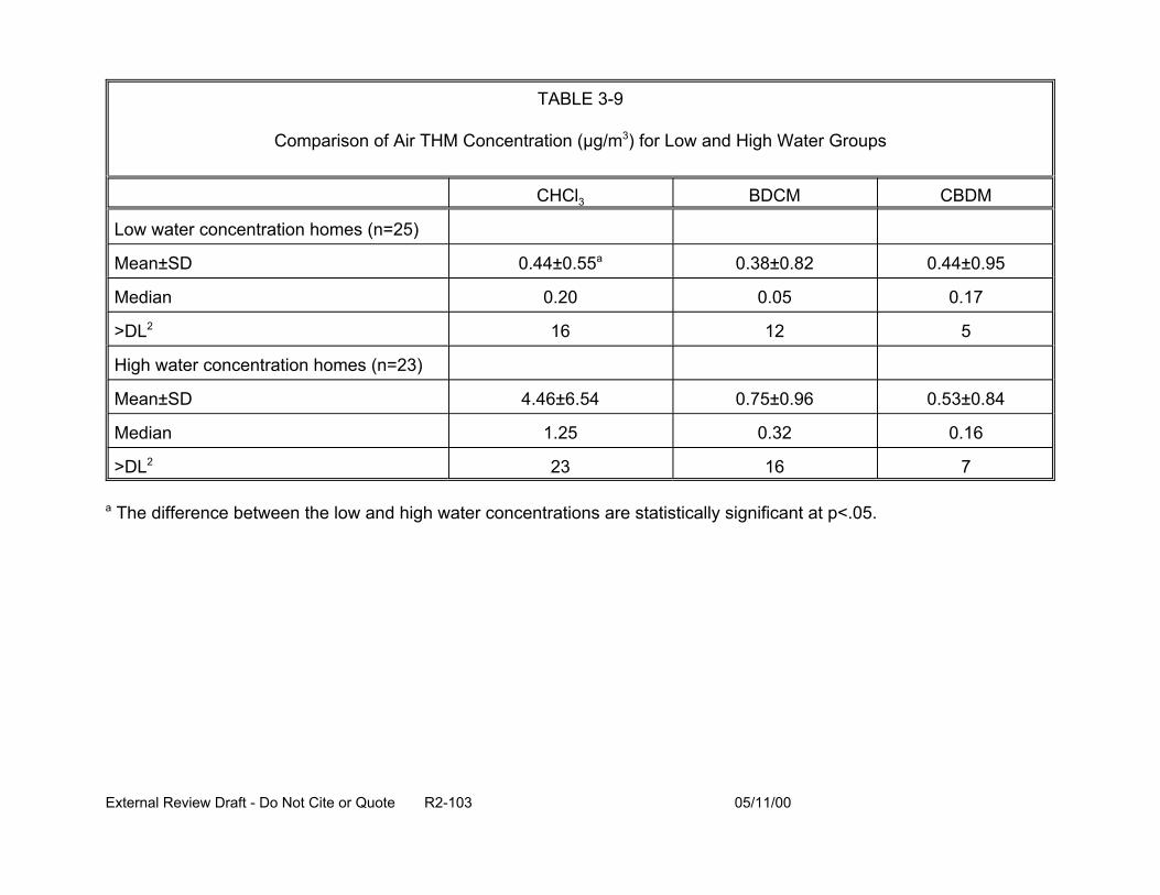
TABLE 3-9
Comparison of Air THM Concentration (µg/m3) for Low and High Water Groups
CHCl3 BDCM CBDM
Low water concentration homes (n=25)
Mean±SD 0.44±0.55a 0.38±0.82 0.44±0.95
Median 0.20 0.05 0.17
>DL2 16 12 5
High water concentration homes (n=23)
Mean±SD 4.46±6.54 0.75±0.96 0.53±0.84
Median 1.25 0.32 0.16
>DL2 23 16 7
a The difference between the low and high water concentrations are statistically significant at p<.05.
External Review Draft - Do Not Cite or Quote R2-103 05/11/00
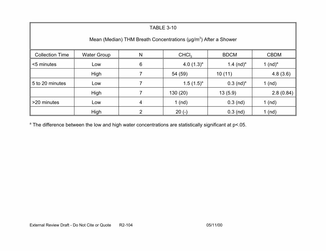
TABLE 3-10
Mean (Median) THM Breath Concentrations (µg/m3) After a Shower
Collection Time Water Group N CHCl3 BDCM CBDM
<5 minutes Low 6 4.0 (1.3)a 1.4 (nd)a 1 (nd)a
High 7 54 (59) 10 (11) 4.8 (3.6)
5 to 20 minutes Low 7 1.5 (1.5)a 0.3 (nd)a 1 (nd)
High 7 130 (20) 13 (5.9) 2.8 (0.84)
>20 minutes Low 4 1 (nd) 0.3 (nd) 1 (nd)
High 2 20 (-) 0.3 (nd) 1 (nd)
a The difference between the low and high water concentrations are statistically significant at p<.05.
External Review Draft - Do Not Cite or Quote R2-104 05/11/00
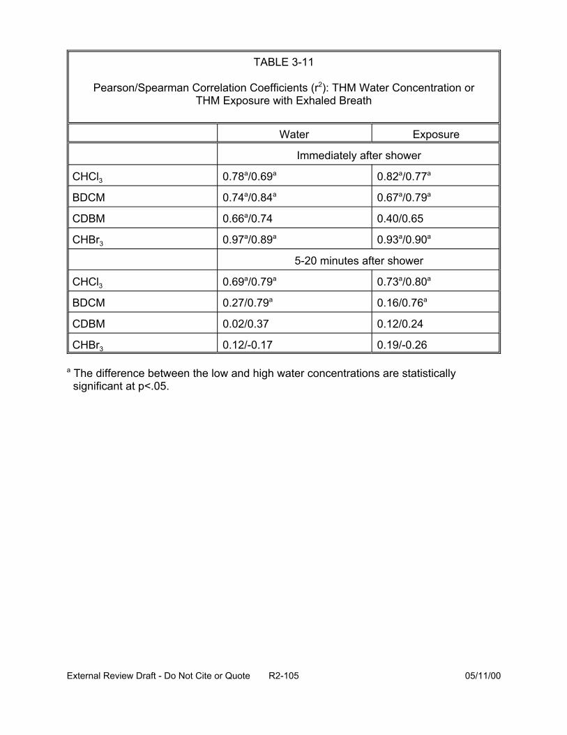
TABLE 3-11
Pearson/Spearman Correlation Coefficients (r2): THM Water Concentration or THM Exposure with Exhaled Breath
Water Exposure
Immediately after shower
CHCl3 0.78a/0.69a 0.82a/0.77a
BDCM 0.74a/0.84a 0.67a/0.79a
CDBM 0.66a/0.74 0.40/0.65
CHBr3 0.97a/0.89a 0.93a/0.90a
5-20 minutes after shower
CHCl3 0.69a/0.79a 0.73a/0.80a
BDCM 0.27/0.79a 0.16/0.76a
CDBM 0.02/0.37 0.12/0.24
CHBr3 0.12/-0.17 0.19/-0.26
a The difference between the low and high water concentrations are statistically significant at p<.05.
External Review Draft - Do Not Cite or Quote R2-105 05/11/00
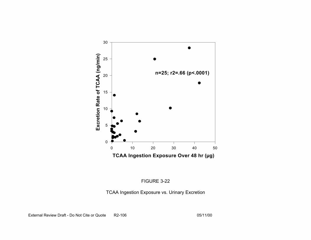
Excr
etio
n R
ate
of T
CA
A (n
g/m
in)
30
25
20
15
10
5
0
n=25; r2=.66 (p<.0001)
0 10 20 30 40
TCAA Ingestion Exposure Over 48 hr (µg)
FIGURE 3-22
TCAA Ingestion Exposure vs. Urinary Excretion
External Review Draft - Do Not Cite or Quote R2-106 05/11/00
50
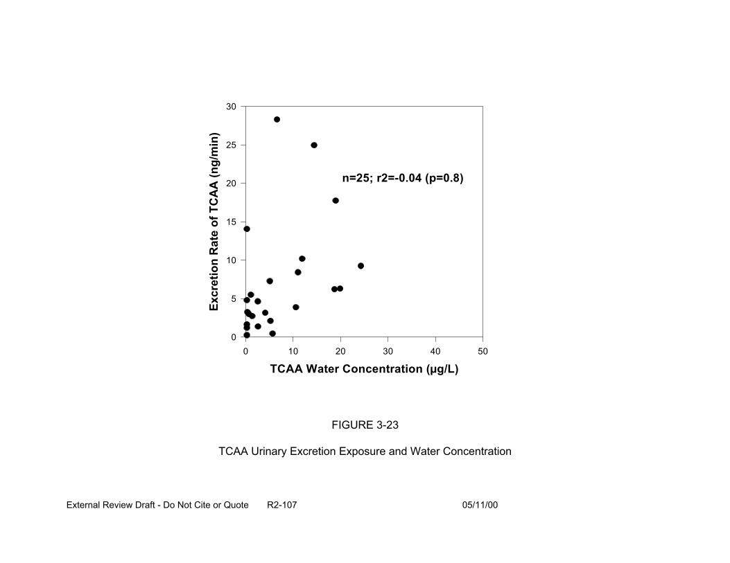
Excr
etio
n R
ate
of T
CA
A (n
g/m
in)
30
25
20
15
10
5
0
n=25; r2=-0.04 (p=0.8)
0 10 20 30 40 50
TCAA Water Concentration (µg/L)
FIGURE 3-23
TCAA Urinary Excretion Exposure and Water Concentration
External Review Draft - Do Not Cite or Quote R2-107 05/11/00
critical. Large variations in ingestion amounts can cause misclassification of exposure
when water concentration is used as a surrogate for exposure if ingestion is the primary
route. For some DBP, inhalation and dermal exposures contribute to the overall dose,
with the relative importance of each route dependent on properties of the particular DBP
(e.g., volatility). Biomarker and exposure/dose models can be used to determine total
exposure in epidemiological studies to reduce misclassification and define routes. The
route of exposure is an important determinant of the kinetics of the DBP (absorption,
distribution, metabolism). The use of water concentration of a specific DBP (e.g., THM)
as an exposure surrogate for all DBP may cause misclassification since the importance
of different exposure routes can vary across compounds. Exposure for selected
agent(s) or DBP(s) may be under-predicted or may not be proportional to the
biologically-active agent.
3.5. PRESENTATION: DBP CONCENTRATION DATA VARIABILITY, ICR DATA (P. Fair)
Disinfectant(s) added to water react with organic material and bromide present in
the source water to form DBP, a wide range of compounds for which only the major
components have been analytically identified. Numerous factors influence DBP
formation, including:
• the disinfectant (what disinfectant is used and its concentration),
• organic material (its chemical nature),
• temperature (affects reaction kinetics, determined by season of the year),
• time (location of sampling, how long the disinfectant has been in contact with organics in the water),
External Review Draft - Do Not Cite or Quote R2-108 05/11/00
• pH (influences the types of by-products), and
• bromide (presence, concentration).
The nature of the organic material that reacts with the disinfectants may vary with
season of the year and the watershed, leading to variability within and between the
water systems. In general, the greater the concentration of organic material, the greater
the formation of by-products.
DBP formed from chlorination include halogenation products (total organic
halides, TOX) and oxidation products because chlorine is a strong oxidizer.
Approximately 20% of the chlorine reacts to form halogenation products while the
remainder goes to oxidizing organic materials. Among the halogenation products are:
THM, HAA, HAN, haloketones (HK), chloral hydrate (CH), and chloropicrin (CP).
Depending on the water, one can account for 10-50% of the TOX following chlorination,
although TOX are highly variable. As there is continued formation of TOX within the
distribution system, TOX and the individual by-product concentrations change with time.
Concentrations are variable, some reactions occur rapidly, and concentrations may
increase with distance (and time) from the treatment facility. Some by-products are also
subject to chemical or microbial degradation and their concentrations may decrease
with distance from the treatment facility. The pH of the water influences the types of by-
products formed following chlorination. With increasing alkalinity, formation of TOX and
haloacetic acids (e.g., TCAA [trichloroacetic acid]) are decreased, but THM formation is
increased. The pH of the water may change during the treatment process, so where the
chlorine is added in the process can greatly influence the types of by-products formed.
The Stage 1 D/DBP Rule will require water systems treating surface water to practice
External Review Draft - Do Not Cite or Quote R2-109 05/11/00
enhanced coagulation which involves lowering the pH during the coagulation process.
Many water systems will need to raise the pH before the water is sent into the
distribution system in order to prevent corrosion and comply with the Lead and Copper
Rule. Bromide concentrations also influence the halogenation reactions. High bromide
concentrations favor the formation of brominated species, whereas at low bromide
concentrations, primarily chlorine substituted by-products are formed. If hypochlorite
solutions instead of gaseous chlorine are used for water treatment, chlorate is added to
the water as a decomposition product present in the hypochlorite solutions.
Alternate disinfectants also lead to the formation of by-products. Chloramination
produces halogenated by products (TOX), cyanogen chloride, cyanogen bromide (in
bromide rich water), oxidation by products, and organic chloramines. Chlorine dioxide is
a strong oxidizer and its use leads to the formation of oxidation products in addition to
the major by-products of chlorite and chlorate. A small amount of halogenated by
products (TOX) may are also be formed. Oxidation products are formed when ozone, a
strong oxidizer, is used for water treatment. If the water source also contains bromide,
then bromine substituted by products and bromate are formed with ozonation.
A study is underway in the U.S. EPA’s Office of Water under the Information
Collection Rule (ICR). The ICR is a data-gathering and evaluation effort wherein data
from all treatment systems serving populations of 100,000 or more persons were
collected. Information on source water characteristics, microbial contamination (in
surface water supplies), DBP and precursor identity and concentration, and treatment
plant design and operation are being compiled and evaluated. In addition, studies are
being conducted to evaluate treatment technologies (e.g., membranes and granulated
External Review Draft - Do Not Cite or Quote R2-110 05/11/00
activated carbon) for precursor removal. The ICR monitored 296 water systems for 18
months (July 1997- December 1998). Monthly data on the treatment plant operation,
water quality parameters and DBP precursors (bromide, UV254, and total organic carbon
[TOC]), and quarterly data on DBP at the entry and terminal points, as well as three
other points, within the distribution system were collected. All plants monitored for
concentrations of THM, HAA, HAN, HK, CP, CH, and TOX. The TOX measurements
provided information on unidentified halogenated products. Specialized data for
alternate disinfection processes were monitored, including: aldehyde and bromate
formation following ozonation (20 plants), cyanogen chloride following chloramination
(184 plants), and aldehydes, bromate, chorite, and chlorate following chlorine dioxide
treatment (32 plants). The monitoring data from the ICR will provide baseline
occurrence data for approximately 500 water treatment plants, refine existing models
used to predict DBP formation, and evaluate how DBP concentrations will change as
treatment changes are implemented.
3.6. PRESENTATION: HUMAN EXPOSURE ESTIMATES: WATER CONSUMPTION (R. Schoeny)
A mandate of the Safe Drinking Water Act (SDWA) Amendments of 1996
requires EPA to identify subpopulations at elevated risk and to conduct studies
characterizing health risk to sensitive populations from contaminants in drinking water.
A population can be considered “sensitive” by virtue of its high exposure (e.g., high
water consumption) or by virtue of its innate or intrinsic sensitivity, due to genotype or
phenotypic characteristics (e.g., immune status).
Consumption of 2 liters/day as a default value for individual water intake is used
widely by federal agencies, including the EPA and the World Health Organization
External Review Draft - Do Not Cite or Quote R2-111 05/11/00
(WHO). This consumption value was based on an analysis of USDA’s 1977-1978
National Food Consumption Study published by Ershow and Cantor (1989). This report
for the National Cancer Institute identified the 90th percentile consumption level to be
about 2 liters of water per day for an adult. However, tap water consumption patterns
have presumably changed during the past 20 years, and the SDWA Amendments
require up-to-date information on water consumption. For example, bottled water was
seldom used in the late 1970's, but now may represent a substantial portion of fluid
intake.
The EPA’s Office of Water has conducted a new analysis of drinking water
consumption which considers multiple water sources. Estimates are stratified by age,
gender, race, socioeconomic status, geographic region, and separately for pregnant
and lactating women. The data source is the USDA’s 1994-1996 Continuing Survey of
Food Intake by Individuals (CSFII). It is expected that the analyses will be applied in
both risk assessment and in the determination of benefits and costs required by the
SDWA amendments. The generation of risk or benefits for specific populations will be
facilitated by use of specific drinking water estimates.
USDA’s 1994-1996 Continuing Survey of Food Intake by Individuals (CSFII) is a
2-day (2 non-consecutive days) dietary intake recall survey of 15,303 respondents. It is
a complex, stratified, multistage, area probability sample of the U.S. population that
includes (by design) over-sampling of low-income population, young children, and the
elderly. In addition to dietary information, some demographic and physical data (e.g.,
body weight) were collected. The CSFII has a response rate of 76%. Surveys are
External Review Draft - Do Not Cite or Quote R2-112 05/11/00
conducted by trained interviewers who use a variety of visual props to assist in
recording of accurate portion sizes.
Specific questions were included in the survey to gather information on the
sources of water consumed by the respondents. Water sources identified in the
analysis included community water supplies (e.g., municipal tap water), bottled water,
and other sources (e.g., well, cistern, spring, etc.). The analyses differentiated between
direct water (plain water consumed directly as a beverage) and indirect water which was
added to foods and beverages during final home or restaurant preparation (e.g., coffee,
tea, reconstituted fruit juice). This analysis did not quantify what was defined as intrinsic
water; that is, water contained in foods and beverages at the time of market purchase
(e.g., canned soup).
There is uncertainty in the analysis. Dietary recall is subjective (e.g., quantity of
food consumed), and it is not known if 2 days is the most appropriate period. Another
source of uncertainty is grounded in the calculation of indirect water from food codes
and the amount of water in foods based on USDA’s standard recipes. In calculating the
amount of water consumed from various sources from questionnaire responses,
assumptions had to be made. The EPA analysis used the following assumptions for
water consumption: all = 100%, most = 75%, some = 25%.
Estimates of water consumption for all age groups and males and females
combined support for the use of a 2 liters/person day default (Table 3-12). The 90th
percentile of community tap water intake is 2.02 liters (across all age groups). In
addition, the preliminary analysis supports the use of 1 liter/day for a 10-kg child. The
External Review Draft - Do Not Cite or Quote R2-113 05/11/00
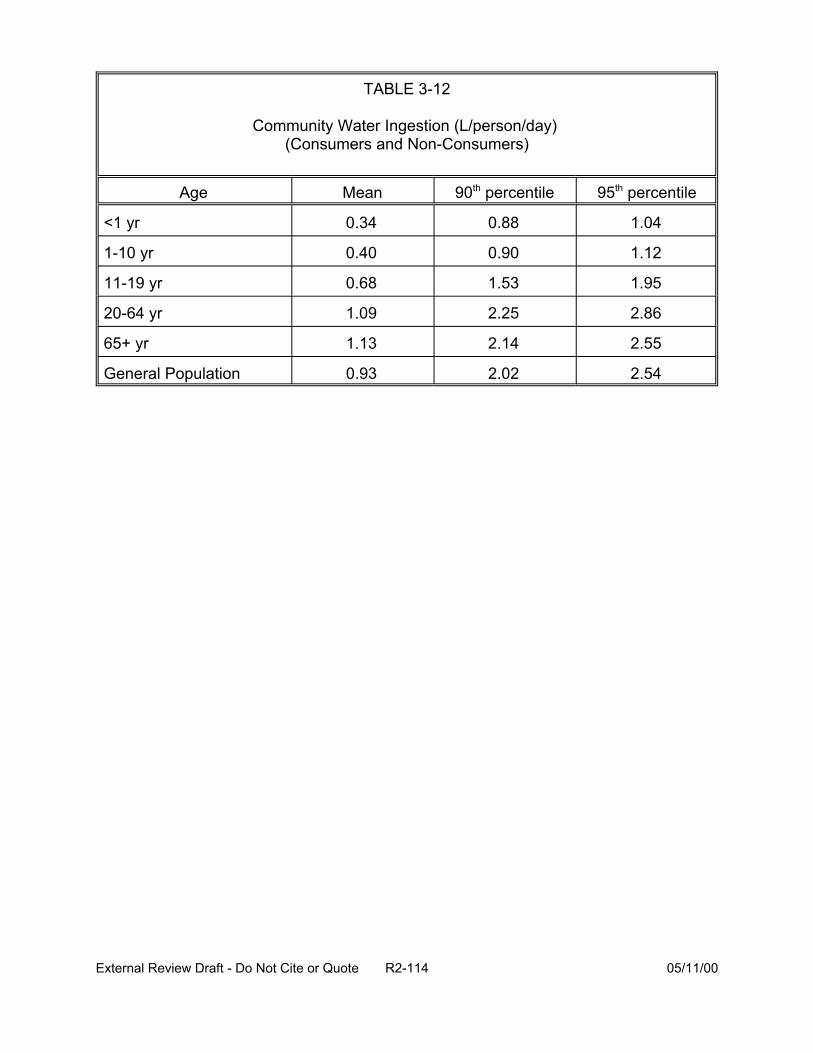
TABLE 3-12
Community Water Ingestion (L/person/day) (Consumers and Non-Consumers)
Age Mean 90th percentile 95th percentile
<1 yr 0.34 0.88 1.04
1-10 yr 0.40 0.90 1.12
11-19 yr 0.68 1.53 1.95
20-64 yr 1.09 2.25 2.86
65+ yr 1.13 2.14 2.55
General Population 0.93 2.02 2.54
External Review Draft - Do Not Cite or Quote R2-114 05/11/00

estimated 95th percentile of community/tap water intake is 1.12 liters for a child 1-10
years old.
Bottled water represents a substantial proportion (13.4%) of combined direct and
indirect water intake. When comparisons were made base on “poverty” or “non-poverty”
status, respondents did not differ substantially in mean intake of tap or bottled water. In
general, males drink more than females, with adolescent males drinking approximately
3 liters/day. Based on per kg body weight, infants (< 1 year old) drink approximately 3
times as much tap water as adults. Lactating women consume, on average,
considerably more tap water than women of child-bearing age. Residents of rural areas
consume, on average, less bottled water and more water from “other” sources, and
residents in the western United States consume more bottled water than other regions.
A report on the analyses has recently been reviewed by the Science Advisory
Board (SAB) to the U.S. EPA. Their preliminary comments indicate that the CSFII data
are an appropriate choice and that the analytic methods used are sound. The report will
be revised and released early in calendar 2000.
3.7. PRESENTATION: PROBABILISTIC APPROACHES TO DEVELOPING DISTRIBUTIONS OF RISKS (W. Huber)
3.7.1. Variability and Uncertainty. Variability is diversity or heterogeneity in a well-
defined population of individuals or series of observations. In risk assessment, the
individuals or observations are usually indexed by time or spatial location or both. For
example, the population exposed to DBP is 170 million people drinking treated water
across the United States within a future (as yet unspecified) time frame. The DBP
concentrations in the treated water also vary with time and location. In the CRFM case
External Review Draft - Do Not Cite or Quote R2-115 05/11/00
study, the concentrations used in the risk assessment are those observed for one week
from one sampling point serving no people (pilot plant).
Variability is related to the experimental situation or question. In general, there
are three different types of variability in risk assessment: population, temporal, and
spatial. There is a “target” population of individuals for whom the risk is being
assessed. The population must be well-defined, i.e., who, what, and when must be
known. Temporal variability is manifested in the variation of concentration or dose over
time (such as DBP concentration at different sampling times). For acute effects,
temporal variation can be very important. Some of the variation within a spatially-
distributed population of individuals can be attributed to spatial locations. Other factors,
such as the concentration term, usually vary with spatial location. (Spatial and temporal
variation often exhibit autocorrelation. Properties of individuals are, however, usually
considered to vary independently of each other.)
Uncertainty, or imperfect knowledge, arises from ignorance or incomplete
information. There are many forms of uncertainty. Some uncertainty is probabilistic,
some uncertainty is in the model, and other uncertainty is “unquantifiable”. The CRFM
divides probabilistic uncertainty into random error and “inherent randomness”. Random
error can be treated statistically. As for inherent randomness, one elects to ignore it
and treats it as a random term in the model (Morgan and Henrion, 1992).
Model uncertainty has many forms that should not or cannot be assessed with
probabilistic approaches, including:
• simplifying assumptions,
• approximations,
External Review Draft - Do Not Cite or Quote R2-116 05/11/00
• degree of empirical validation,
• amount of extrapolation, and
• amount of detail.
Forms of unquantifiable uncertainty, which cannot be assessed numerically, are:
• “lack of empirical basis”,
• subjective judgment,
• linguistic imprecision (such as data from an ambiguous report),
• disagreement (such as to which model to apply),
• systematic error, and
• “data uncertainty”.
All of the components of uncertainty need to be identified before bounds can be
placed on the total uncertainty.
The concepts of variability and uncertainty overlap and are frequently a function
of the choice of models.
Probabilistic techniques use distributions. Frequency distributions and probability
distributions are the same mathematical object. Almost all variability can be
represented by frequency distributions. Only “random” forms of uncertainty can be
represented by probability distributions. In many cases, the uncertainty that can be
probabilistically quantified is dwarfed by the other kinds of uncertainty. Every effort
should be made to identify numerical bounds on the magnitude of the “unquantifiable”
components. Many of the “unquantifiable” uncertainties may cancel out (through
negative covariation or by sharing a common additive component) in a comparative risk
assessment. For example, the comparison of chlorination-filtration with ozonation-
External Review Draft - Do Not Cite or Quote R2-117 05/11/00
chlorination-filtration subtracts many components of uncertainty common to both
treatment methods. Thus, using some models, one may be able to factor out some
uncertainty.
3.7.2. Maximum Likelihood Estimation. When one has data and needs to make
decisions based on those data, a rational decision theory framework can be applied. In
this framework, there is a state space of possible outcomes of a random variable.
There is a set of distributions representing realistic states of nature. The set of possible
decisions is specified. A loss function specifying the costs for a bad decisions must be
known. Optionally, one may also specify an a priori probability distribution of the states
of nature.
Within this framework, and independent of it, there are many criteria for choosing
or evaluating a decision procedure. Among them are:
• maximum likelihood and likelihood ratio,
• Bayes,
• minimax,
• invariance,
• unbiasedness,
• sufficiency,
• robustness,
• method of moments, and
• asymptotic efficiency.
External Review Draft - Do Not Cite or Quote R2-118 05/11/00
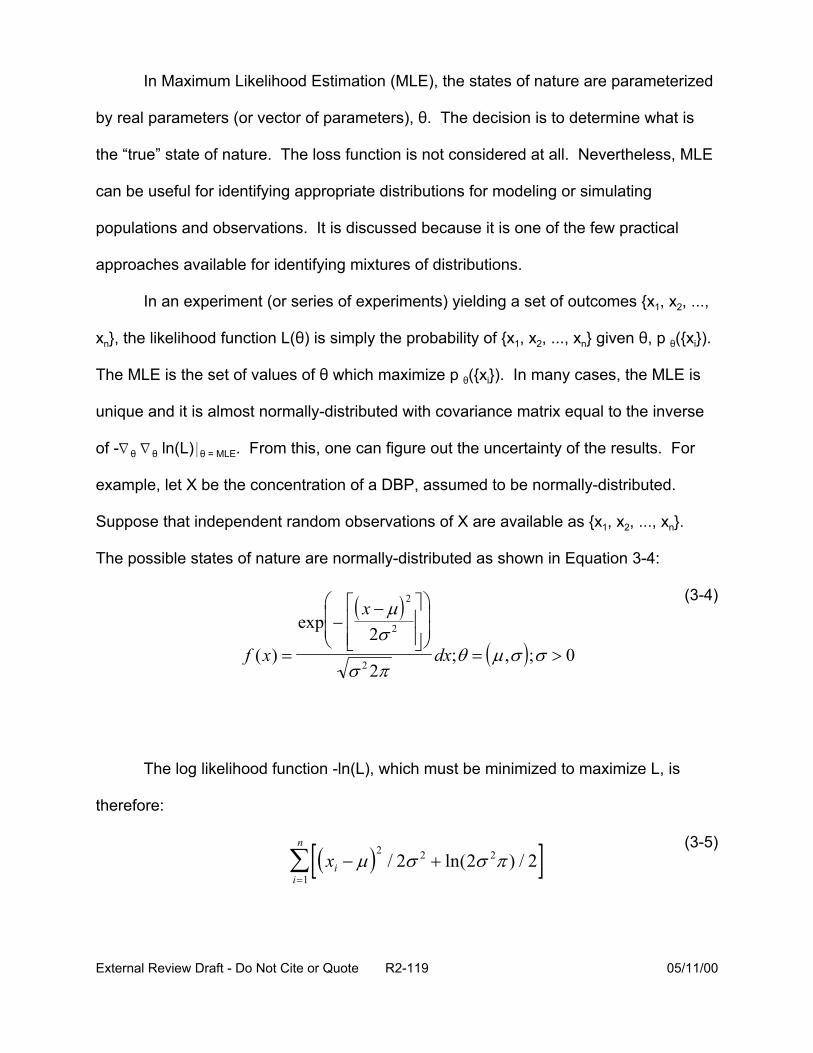
f x
In Maximum Likelihood Estimation (MLE), the states of nature are parameterized
by real parameters (or vector of parameters), 2. The decision is to determine what is
the “true” state of nature. The loss function is not considered at all. Nevertheless, MLE
can be useful for identifying appropriate distributions for modeling or simulating
populations and observations. It is discussed because it is one of the few practical
approaches available for identifying mixtures of distributions.
In an experiment (or series of experiments) yielding a set of outcomes {x1, x2, ...,
xn}, the likelihood function L(2) is simply the probability of {x1, x2, ..., xn} given 2, p 2({xi}).
The MLE is the set of values of 2 which maximize p 2({xi}). In many cases, the MLE is
unique and it is almost normally-distributed with covariance matrix equal to the inverse
of -L 2 L 2 ln(L)* 2 = MLE. From this, one can figure out the uncertainty of the results. For
example, let X be the concentration of a DBP, assumed to be normally-distributed.
Suppose that independent random observations of X are available as {x1, x2, ..., xn}.
The possible states of nature are normally-distributed as shown in Equation 3-4:
( x − µ) 2 (3-4)
( ) = σ π2 2
exp−
2σ 2
dx;θ = (µ,σ );σ > 0
The log likelihood function -ln(L), which must be minimized to maximize L, is
therefore:
n (3-5)∑[(xi − µ)2
/ 2σ 2 + ln(2σ 2π ) / 2]i =1
External Review Draft - Do Not Cite or Quote R2-119 05/11/00
A unique minimum occurs where : = arithmetic mean of {xi} and F = standard
deviation of {xi} (provided this is nonzero).
One can also find the so-called “second order uncertainty” with MLE. The
estimated values of : and F are independent with variances of F2 /n and 2F2 /n,
respectively. When n is large enough, these variances approximately characterize the
uncertainty distributions of : and F. Thus, MLE simultaneously yields estimates of
variability (in the form of F2) and uncertainty (in the form of the uncertainty distribution of
: and F).
Some advantages and disadvantages of MLE are listed in Table 3-13. Maximum
likelihood works well with lots of data and serves to complement Monte Carlo
techniques as a means to separate uncertainty and variability.
3.7.3. Mixtures of Distributions. Mixtures of parameterized distributions can be used
as an alternative to assuming one nice mathematical distribution (such as normal or
lognormal). Mixtures of distributions arise in nature, such as the National Inorganic and
Radionuclides Survey (NIRS) data base of radon measurements in drinking water. The
probability plots suggest that these data are only approximately characterized by a
lognormal distribution. The approximation is poorest where it often matters the most- in
the high-concentration “tail” of the distribution (See Figures 3-24, 3-25, and 3-26.).
The definition of a mixed distribution is as follows:
• Let f1(X; 21),..., fk(X; 2k), be a sequence of probability distribution functions. X is the variate and the {2k} are the parameters.
• Let B1, ...,Bk be a sequence of strictly positive real numbers with B1+ ...+Bk + 1. Then B1f1(X; 21) + ... + Bkfk (X;2k) is a finite mixture distribution.
External Review Draft - Do Not Cite or Quote R2-120 05/11/00
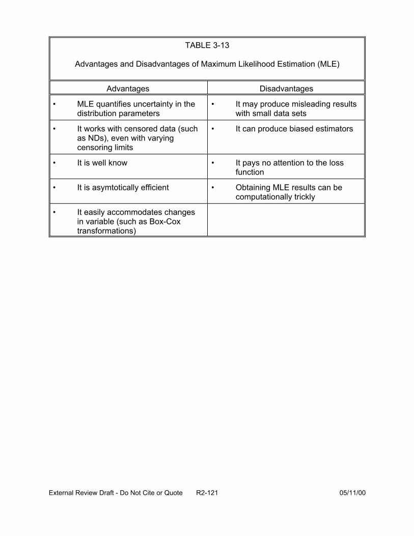
TABLE 3-13
Advantages and Disadvantages of Maximum Likelihood Estimation (MLE)
Advantages Disadvantages
• MLE quantifies uncertainty in the • It may produce misleading results distribution parameters with small data sets
• It works with censored data (such as NDs), even with varying censoring limits
• It can produce biased estimators
• It is well know • It pays no attention to the loss function
• It is asymtotically efficient • Obtaining MLE results can be computationally trickly
• It easily accommodates changes in variable (such as Box-Cox transformations)
External Review Draft - Do Not Cite or Quote R2-121 05/11/00
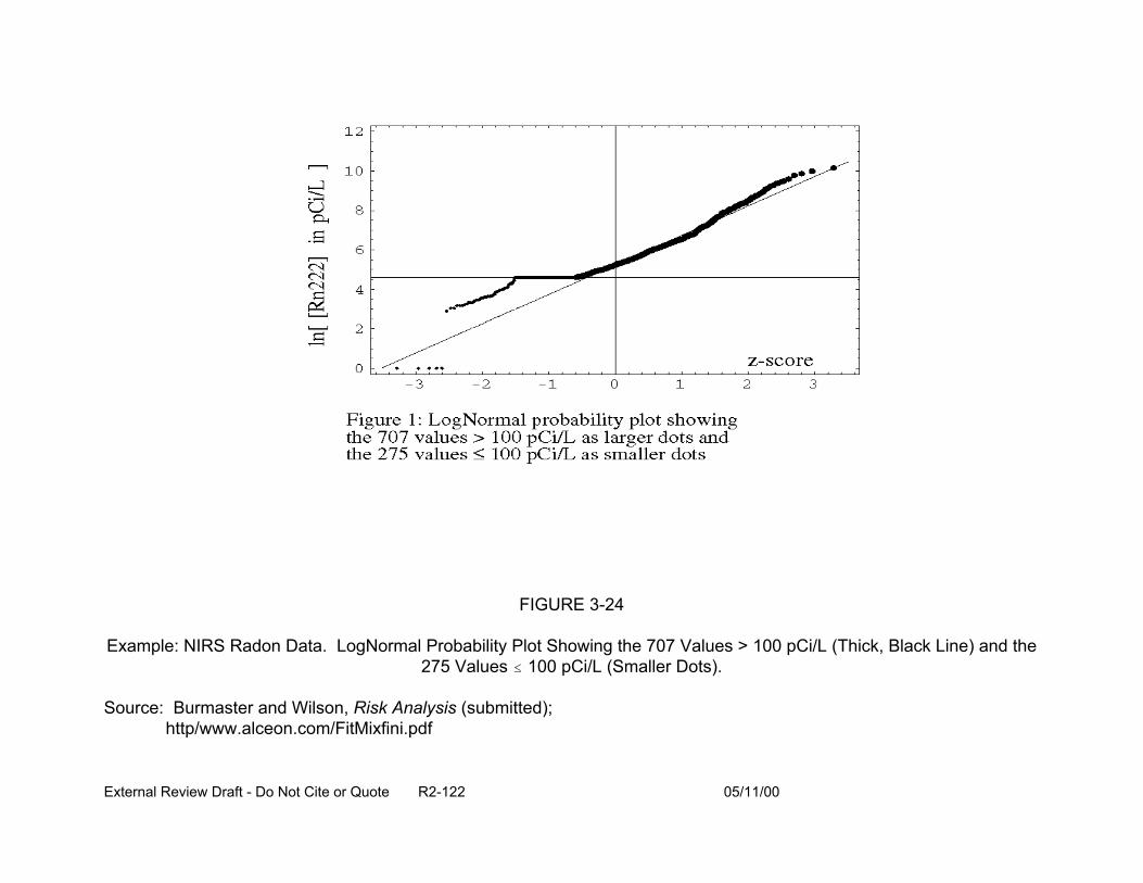
FIGURE 3-24
Example: NIRS Radon Data. LogNormal Probability Plot Showing the 707 Values > 100 pCi/L (Thick, Black Line) and the 275 Values # 100 pCi/L (Smaller Dots).
Source: Burmaster and Wilson, Risk Analysis (submitted); http/www.alceon.com/FitMixfini.pdf
External Review Draft - Do Not Cite or Quote R2-122 05/11/00
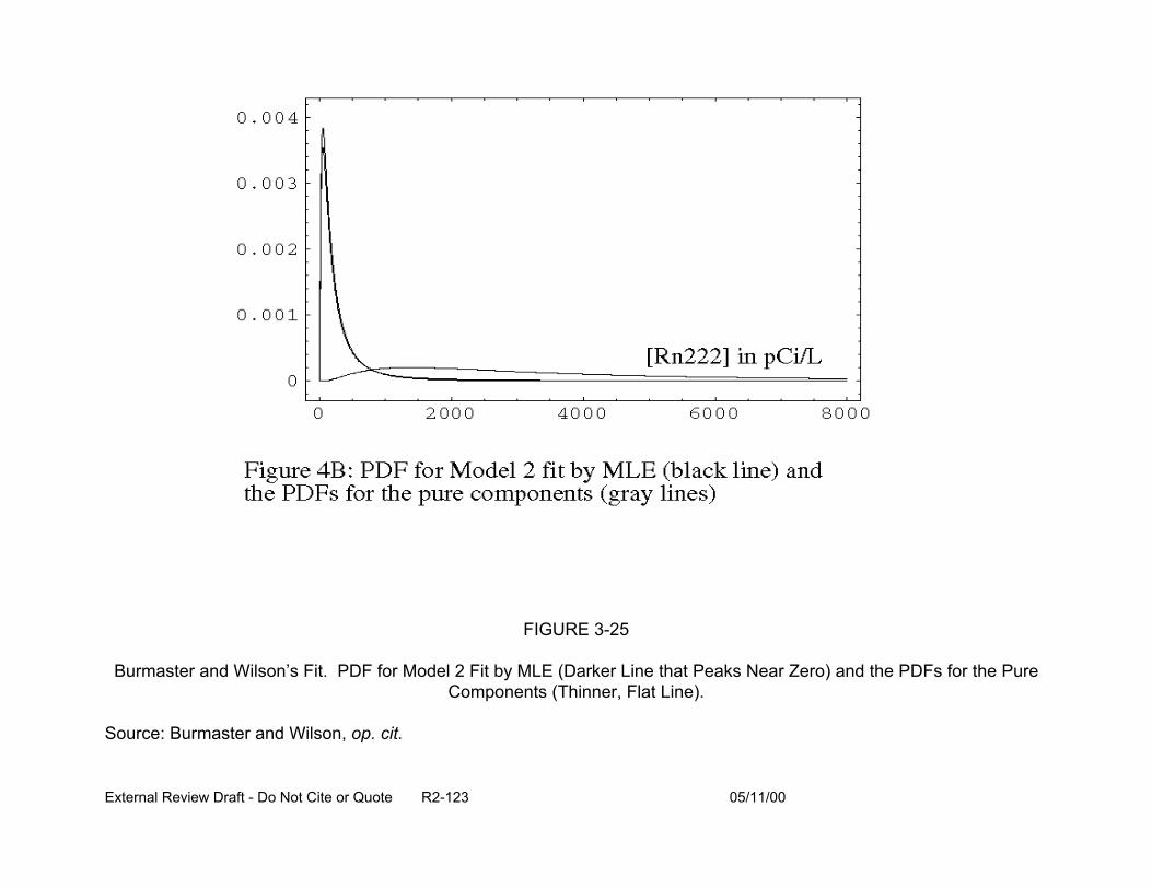
FIGURE 3-25
Burmaster and Wilson’s Fit. PDF for Model 2 Fit by MLE (Darker Line that Peaks Near Zero) and the PDFs for the Pure Components (Thinner, Flat Line).
Source: Burmaster and Wilson, op. cit.
External Review Draft - Do Not Cite or Quote R2-123 05/11/00
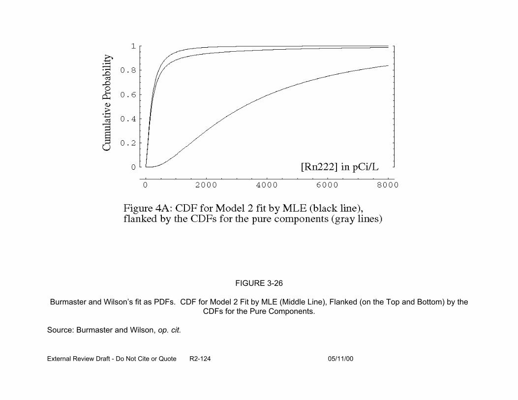
FIGURE 3-26
Burmaster and Wilson’s fit as PDFs. CDF for Model 2 Fit by MLE (Middle Line), Flanked (on the Top and Bottom) by the CDFs for the Pure Components.
Source: Burmaster and Wilson, op. cit.
External Review Draft - Do Not Cite or Quote R2-124 05/11/00

Mixture distributions have advantages over mathematically simpler distributions: they
expand the range of available distributions for fitting data; they often correspond better
to real phenomena; and they can model “surprise” and rare events. Use of mixture
distributions and MLE offer advantages in that uncertainty in the mixing parameters
B1, ...,Bk is quantified, the MLE can assess whether a component is statistically
significant, and the MLE is one of the few ways to make estimates with general mixture
models.
However, there are several difficulties in using MLE for estimates in a mixture
model framework. Deciding how many mixture components should be used is an issue
with this approach. Another issue is that solutions to the MLE equations can be difficult
to find or may be numerically unstable since ln(L) is almost parabolic near its maxima.
One way to determine the number of components is a graphical technique, the
mixture diagnostic plot (MDP), developed by Roeder (1994), as depicted in Figure 3-27.
The MDP is a graphical expression of a formal hypothesis test of whether the number of
normal components in a mixture is k (k > 1) or k + 1. (It assumes each component of
the mixture has the same spread.) The test is based on the number of sign changes
found in comparing a nonparametric smooth of the empirical density function to a k-
component fit to the data.
In the figures (Figures 3-24, 3-25, and 3-26) of the NIRS data, the smoothed
(empirical) distribution appears to depart somewhat from the best-fitting lognormal
distribution. The smooth may have some “bumps”, but they are small. Roeder’s MDP,
in both the graphical form (shown in Figure 3-27) and as a statistical test, support the
alternative hypothesis of (at least) two components to the data and reject the null
External Review Draft - Do Not Cite or Quote R2-125 05/11/00
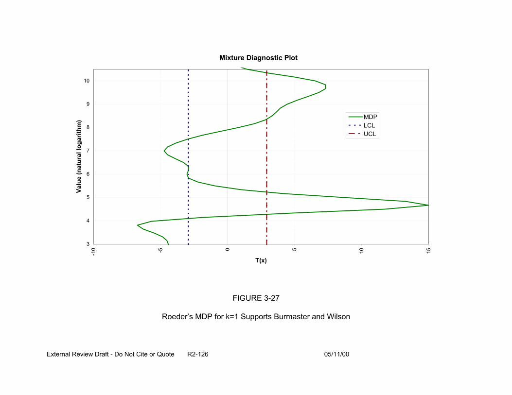
10
9
8
7
6
5
4
3
MDP LCL UCL
Mixture Diagnostic Plot
T(x)
FIGURE 3-27
Roeder’s MDP for k=1 Supports Burmaster and Wilson
Valu
e (n
atur
al lo
garit
hm)
-10 -5 0 5 10
15
External Review Draft - Do Not Cite or Quote R2-126 05/11/00
hypothesis of just one component (k=1). This supports conclusions reached by
Burmaster and Wilson independently using other techniques (to appear in Risk
Analysis).
The MDP is more general than indicated here. It can be developed for any
number of components. It does not require that the empirical distribution have any
multiple “bumps” at all; in other words, it can detect mixtures of distributions that are so
close they are not multimodal. The MDP works directly for mixtures of lognormals (just
take logarithms). Unfortunately, computing the significance levels for the corresponding
statistical test (the mixtures diagnostic test, MDT) requires Monte Carlo simulation.
3.7.4. Summary. In conclusion, not all uncertainty can be quantified probabilistically.
Indeed, perhaps very little of it can be. MLE and mixtures of distributions can enhance
the ability to capture more uncertainty quantitatively. The results are directly useful for
two-dimensional Monte Carlo simulations. Mixtures of distributions enable better
characterization of important tails of empirical distributions. This approach to
characterizing distributions looks particularly promising for characterizing risks from
DBP in drinking water.
3.8. PRESENTATION: PROPORTIONAL RESPONSE ADDITION (W. Stiteler)
3.8.1. Introduction. Quantification of the risk associated with the low level of exposure
to individual components in a complex mixture of DBP (i.e., a mixture with a large
number of DBP) presents a difficult challenge. For some components, there may not be
toxicity information available. For a particular (noncancer) endpoint, the exposure may
be well below threshold for each of the individual components. Adding these
External Review Draft - Do Not Cite or Quote R2-127 05/11/00
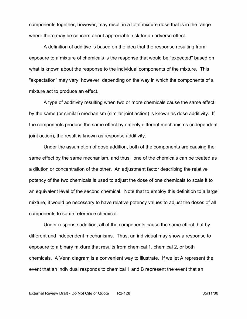
components together, however, may result in a total mixture dose that is in the range
where there may be concern about appreciable risk for an adverse effect.
A definition of additive is based on the idea that the response resulting from
exposure to a mixture of chemicals is the response that would be "expected" based on
what is known about the response to the individual components of the mixture. This
"expectation" may vary, however, depending on the way in which the components of a
mixture act to produce an effect.
A type of additivity resulting when two or more chemicals cause the same effect
by the same (or similar) mechanism (similar joint action) is known as dose additivity. If
the components produce the same effect by entirely different mechanisms (independent
joint action), the result is known as response additivity.
Under the assumption of dose addition, both of the components are causing the
same effect by the same mechanism, and thus, one of the chemicals can be treated as
a dilution or concentration of the other. An adjustment factor describing the relative
potency of the two chemicals is used to adjust the dose of one chemicals to scale it to
an equivalent level of the second chemical. Note that to employ this definition to a large
mixture, it would be necessary to have relative potency values to adjust the doses of all
components to some reference chemical.
Under response addition, all of the components cause the same effect, but by
different and independent mechanisms. Thus, an individual may show a response to
exposure to a binary mixture that results from chemical 1, chemical 2, or both
chemicals. A Venn diagram is a convenient way to illustrate. If we let A represent the
event that an individual responds to chemical 1 and B represent the event that an
External Review Draft - Do Not Cite or Quote R2-128 05/11/00
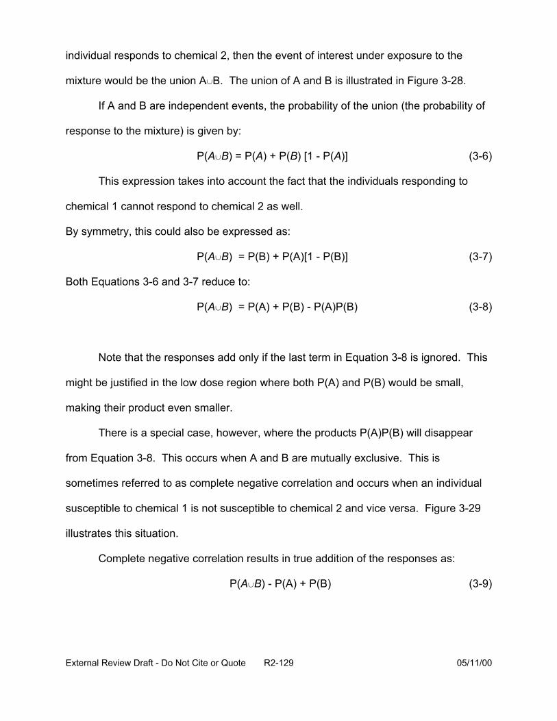
individual responds to chemical 2, then the event of interest under exposure to the
mixture would be the union AcB. The union of A and B is illustrated in Figure 3-28.
If A and B are independent events, the probability of the union (the probability of
response to the mixture) is given by:
P(AcB) = P(A) + P(B) [1 - P(A)] (3-6)
This expression takes into account the fact that the individuals responding to
chemical 1 cannot respond to chemical 2 as well.
By symmetry, this could also be expressed as:
P(AcB) = P(B) + P(A)[1 - P(B)]
Both Equations 3-6 and 3-7 reduce to:
P(AcB) = P(A) + P(B) - P(A)P(B)
(3-7)
(3-8)
Note that the responses add only if the last term in Equation 3-8 is ignored. This
might be justified in the low dose region where both P(A) and P(B) would be small,
making their product even smaller.
There is a special case, however, where the products P(A)P(B) will disappear
from Equation 3-8. This occurs when A and B are mutually exclusive. This is
sometimes referred to as complete negative correlation and occurs when an individual
susceptible to chemical 1 is not susceptible to chemical 2 and vice versa. Figure 3-29
illustrates this situation.
Complete negative correlation results in true addition of the responses as:
P(AcB) - P(A) + P(B) (3-9)
External Review Draft - Do Not Cite or Quote R2-129 05/11/00
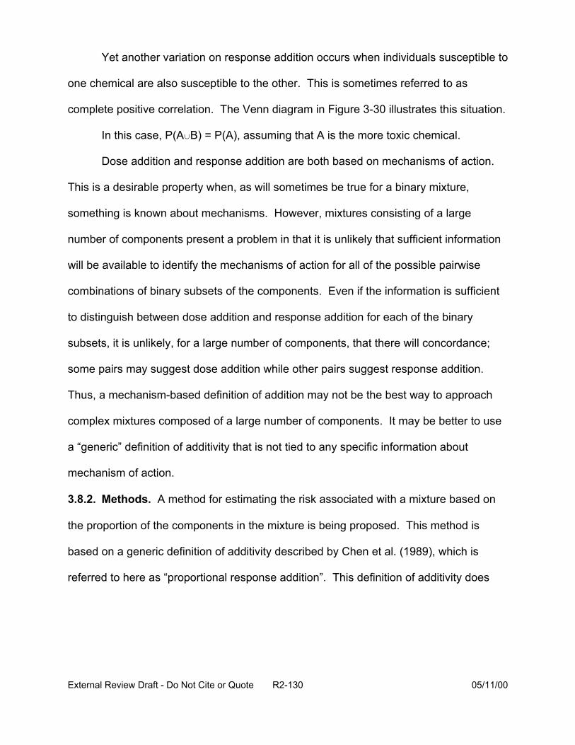
Yet another variation on response addition occurs when individuals susceptible to
one chemical are also susceptible to the other. This is sometimes referred to as
complete positive correlation. The Venn diagram in Figure 3-30 illustrates this situation.
In this case, P(AcB) = P(A), assuming that A is the more toxic chemical.
Dose addition and response addition are both based on mechanisms of action.
This is a desirable property when, as will sometimes be true for a binary mixture,
something is known about mechanisms. However, mixtures consisting of a large
number of components present a problem in that it is unlikely that sufficient information
will be available to identify the mechanisms of action for all of the possible pairwise
combinations of binary subsets of the components. Even if the information is sufficient
to distinguish between dose addition and response addition for each of the binary
subsets, it is unlikely, for a large number of components, that there will concordance;
some pairs may suggest dose addition while other pairs suggest response addition.
Thus, a mechanism-based definition of addition may not be the best way to approach
complex mixtures composed of a large number of components. It may be better to use
a “generic” definition of additivity that is not tied to any specific information about
mechanism of action.
3.8.2. Methods. A method for estimating the risk associated with a mixture based on
the proportion of the components in the mixture is being proposed. This method is
based on a generic definition of additivity described by Chen et al. (1989), which is
referred to here as “proportional response addition”. This definition of additivity does
External Review Draft - Do Not Cite or Quote R2-130 05/11/00
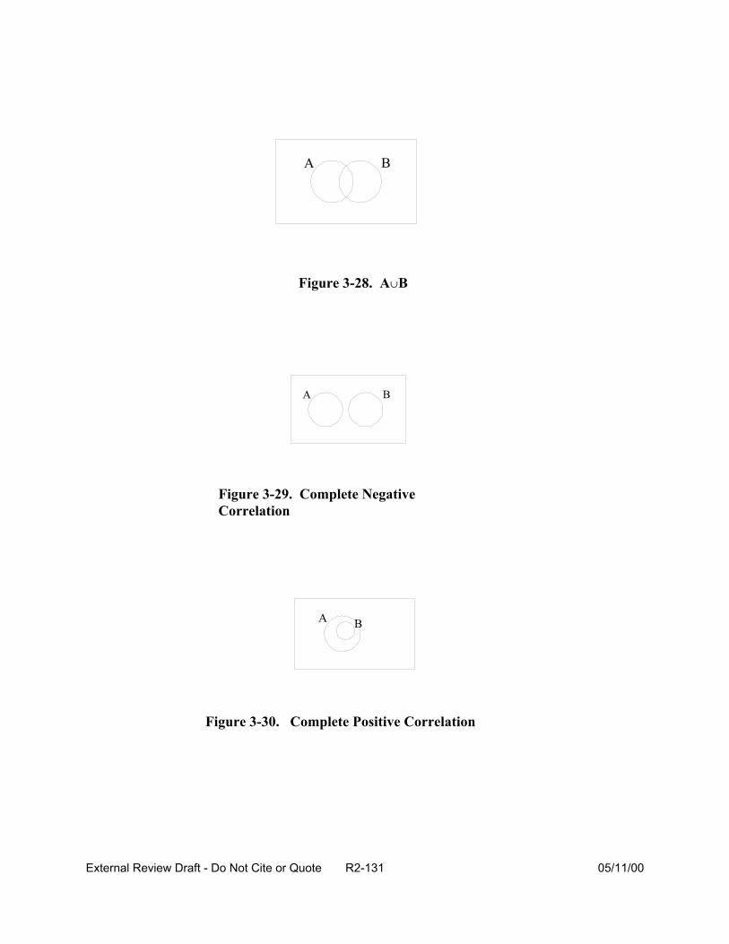
Figure 3-28. AcB
Figure 3-29. Complete Negative Correlation
Figure 3-30. Complete Positive Correlation
External Review Draft - Do Not Cite or Quote R2-131 05/11/00
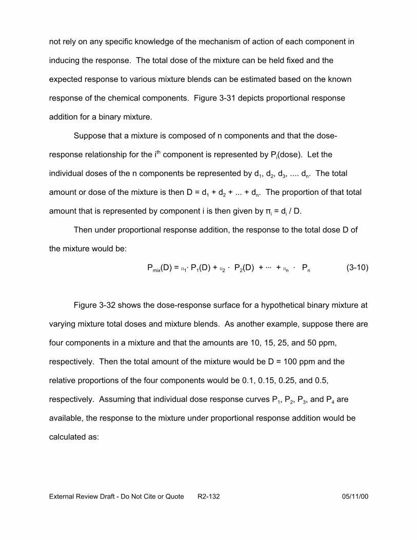
not rely on any specific knowledge of the mechanism of action of each component in
inducing the response. The total dose of the mixture can be held fixed and the
expected response to various mixture blends can be estimated based on the known
response of the chemical components. Figure 3-31 depicts proportional response
addition for a binary mixture.
Suppose that a mixture is composed of n components and that the dose-
response relationship for the ith component is represented by Pi(dose). Let the
individual doses of the n components be represented by d1, d2, d3, .... dn. The total
amount or dose of the mixture is then D = d1 + d2 + ... + dn. The proportion of that total
amount that is represented by component i is then given by Bi = di / D.
Then under proportional response addition, the response to the total dose D of
the mixture would be:
Pmix(D) = (1@ P1(D) + (2 @ P2(D) + @@@ + (n @ Pn (3-10)
Figure 3-32 shows the dose-response surface for a hypothetical binary mixture at
varying mixture total doses and mixture blends. As another example, suppose there are
four components in a mixture and that the amounts are 10, 15, 25, and 50 ppm,
respectively. Then the total amount of the mixture would be D = 100 ppm and the
relative proportions of the four components would be 0.1, 0.15, 0.25, and 0.5,
respectively. Assuming that individual dose response curves P1, P2, P3, and P4 are
available, the response to the mixture under proportional response addition would be
calculated as:
External Review Draft - Do Not Cite or Quote R2-132 05/11/00

Figure 3-31. Proportional Response Addition (Total Dose Held Fixed)
External Review Draft - Do Not Cite or Quote R2-133 05/11/00

FIGURE 3-32
Linear Model Evaluated at d1 and at d1 + d2
External Review Draft - Do Not Cite or Quote R2-134 05/11/00
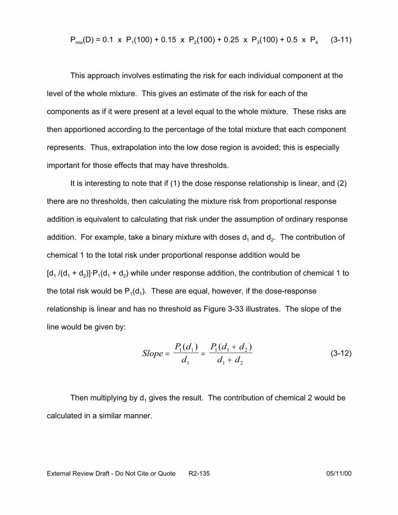
Pmix(D) = 0.1 x P1(100) + 0.15 x P2(100) + 0.25 x P3(100) + 0.5 x P4 (3-11)
This approach involves estimating the risk for each individual component at the
level of the whole mixture. This gives an estimate of the risk for each of the
components as if it were present at a level equal to the whole mixture. These risks are
then apportioned according to the percentage of the total mixture that each component
represents. Thus, extrapolation into the low dose region is avoided; this is especially
important for those effects that may have thresholds.
It is interesting to note that if (1) the dose response relationship is linear, and (2)
there are no thresholds, then calculating the mixture risk from proportional response
addition is equivalent to calculating that risk under the assumption of ordinary response
addition. For example, take a binary mixture with doses d1 and d2. The contribution of
chemical 1 to the total risk under proportional response addition would be
[d1 /(d1 + d2)]@P1(d1 + d2) while under response addition, the contribution of chemical 1 to
the total risk would be P1(d1). These are equal, however, if the dose-response
relationship is linear and has no threshold as Figure 3-33 illustrates. The slope of the
line would be given by:
1( ) 1 (Slope =
P d1 = P d1 + d2 )
(3-12)d1 d1 + d2
Then multiplying by d1 gives the result. The contribution of chemical 2 would be
calculated in a similar manner.
External Review Draft - Do Not Cite or Quote R2-135 05/11/00
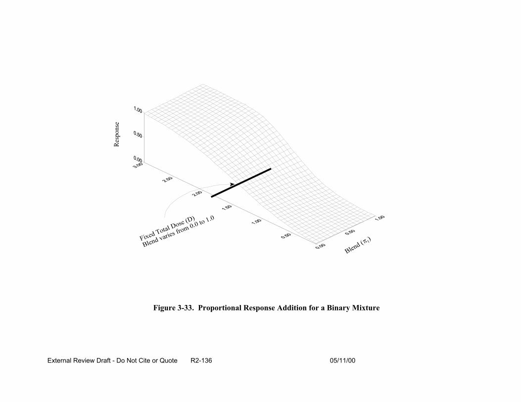
Figure 3-33. Proportional Response Addition for a Binary Mixture
External Review Draft - Do Not Cite or Quote R2-136 05/11/00
Note that if the dose-response function for the first component has a threshold,
then it is possible that P1(d1) = 0.0 while P1(d1 + d2) > 0.0. In that case, the two methods
would lead to different estimates of risk.
Thus, under conditions that might be encountered with a non-threshold endpoint
(e.g., cancer) where exposures are in the linear portion of the dose-response curve,
proportional response addition and response addition would result in identical risk
estimates.
The developmental and reproductive health risks for two classes of DBP, the
haloacetic acids and the haloacetonitriles, were evaluated to serve as an example for
illustration of the proportional response additivity methodology. The haloacetic acids
and haloacetonitriles commonly found in drinking water are listed in Table 3-14. The
table shows the chemical name, formula, and acronyms used in this presentation. In
addition, the table presents a indication of the availability of developmental and
reproductive toxicity data. Seven of the eleven haloacetic acids (MCA, DCA, TCA,
MCA) and haloacetonitriles (DCAN, TCAN, BCAN) have been subjects of
developmental toxicity studies by a single group of investigators, and three of the
haloacetic acids (DCA, MBA, DBA) have been the subjects of male reproductive studies
by another group of investigators. All of these studies were conducted in rats using
gavage administration. The results for developmental toxicity were positive. For
reproductive toxicity, the dihalogenated haloacetic acids gave positive results, but the
monohalogenated acetic acid (MBA) gave negative results. An additional chemical, the
haloacetonitrile DBAN, was tested in a short-term developmental and reproductive
toxicity screening study in rats by the NTP (1992), with negative results. DBAN was
External Review Draft - Do Not Cite or Quote R2-137 05/11/00
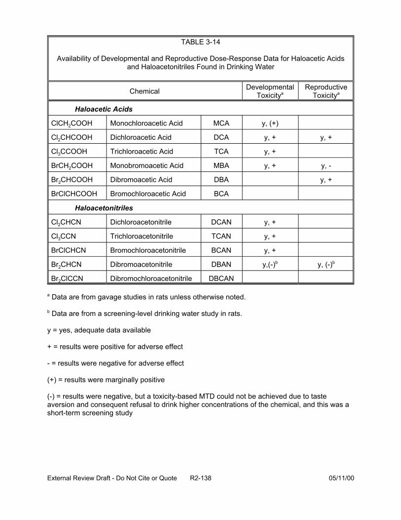
TABLE 3-14
Availability of Developmental and Reproductive Dose-Response Data for Haloacetic Acids and Haloacetonitriles Found in Drinking Water
Chemical
Haloacetic Acids
ClCH2COOH Monochloroacetic Acid MCA y, (+)
Cl2CHCOOH Dichloroacetic Acid DCA y, + y, +
Cl3CCOOH Trichloroacetic Acid TCA y, +
BrCH2COOH Monobromoacetic Acid MBA y, + y, -
Br2CHCOOH Dibromoacetic Acid DBA y, +
BrClCHCOOH Bromochloroacetic Acid BCA
Haloacetonitriles
Cl2CHCN Dichloroacetonitrile DCAN y, +
Cl3CCN Trichloroacetonitrile TCAN y, +
BrClCHCN Bromochloroacetonitrile BCAN y, +
Br2CHCN Dibromoacetonitrile DBAN y,(-)b y, (-)b
Br2ClCCN Dibromochloroacetonitrile DBCAN
a Data are from gavage studies in rats unless otherwise noted.
b Data are from a screening-level drinking water study in rats.
y = yes, adequate data available
+ = results were positive for adverse effect
- = results were negative for adverse effect
(+) = results were marginally positive
Developmental Toxicitya
Reproductive Toxicitya
(-) = results were negative, but a toxicity-based MTD could not be achieved due to taste aversion and consequent refusal to drink higher concentrations of the chemical, and this was a short-term screening study
External Review Draft - Do Not Cite or Quote R2-138 05/11/00
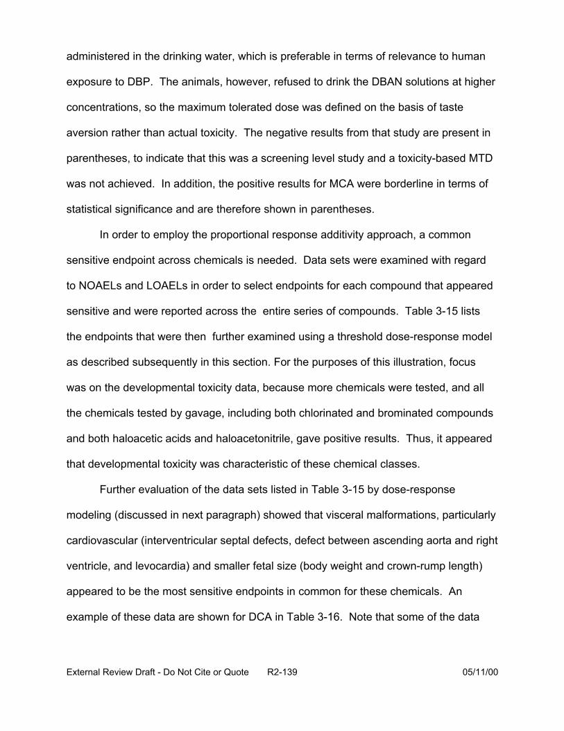
administered in the drinking water, which is preferable in terms of relevance to human
exposure to DBP. The animals, however, refused to drink the DBAN solutions at higher
concentrations, so the maximum tolerated dose was defined on the basis of taste
aversion rather than actual toxicity. The negative results from that study are present in
parentheses, to indicate that this was a screening level study and a toxicity-based MTD
was not achieved. In addition, the positive results for MCA were borderline in terms of
statistical significance and are therefore shown in parentheses.
In order to employ the proportional response additivity approach, a common
sensitive endpoint across chemicals is needed. Data sets were examined with regard
to NOAELs and LOAELs in order to select endpoints for each compound that appeared
sensitive and were reported across the entire series of compounds. Table 3-15 lists
the endpoints that were then further examined using a threshold dose-response model
as described subsequently in this section. For the purposes of this illustration, focus
was on the developmental toxicity data, because more chemicals were tested, and all
the chemicals tested by gavage, including both chlorinated and brominated compounds
and both haloacetic acids and haloacetonitrile, gave positive results. Thus, it appeared
that developmental toxicity was characteristic of these chemical classes.
Further evaluation of the data sets listed in Table 3-15 by dose-response
modeling (discussed in next paragraph) showed that visceral malformations, particularly
cardiovascular (interventricular septal defects, defect between ascending aorta and right
ventricle, and levocardia) and smaller fetal size (body weight and crown-rump length)
appeared to be the most sensitive endpoints in common for these chemicals. An
example of these data are shown for DCA in Table 3-16. Note that some of the data
External Review Draft - Do Not Cite or Quote R2-139 05/11/00
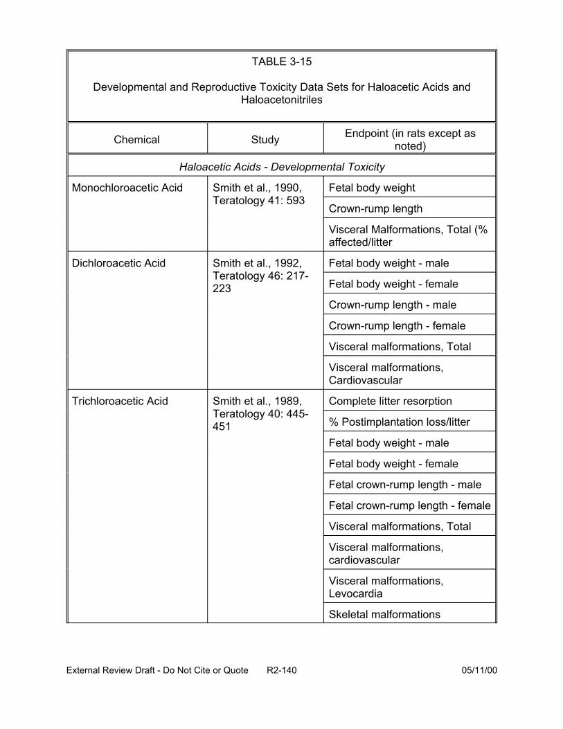
TABLE 3-15
Developmental and Reproductive Toxicity Data Sets for Haloacetic Acids and Haloacetonitriles
Chemical Study Endpoint (in rats except as noted)
Haloacetic Acids - Developmental Toxicity
Monochloroacetic Acid Smith et al., 1990, Teratology 41: 593
Fetal body weight
Crown-rump length
Visceral Malformations, Total (% affected/litter
Dichloroacetic Acid Smith et al., 1992, Teratology 46: 217-223
Fetal body weight - male
Fetal body weight - female
Crown-rump length - male
Crown-rump length - female
Visceral malformations, Total
Visceral malformations, Cardiovascular
Trichloroacetic Acid Smith et al., 1989, Teratology 40: 445-451
Complete litter resorption
% Postimplantation loss/litter
Fetal body weight - male
Fetal body weight - female
Fetal crown-rump length - male
Fetal crown-rump length - female
Visceral malformations, Total
Visceral malformations, cardiovascular
Visceral malformations, Levocardia
Skeletal malformations
External Review Draft - Do Not Cite or Quote R2-140 05/11/00
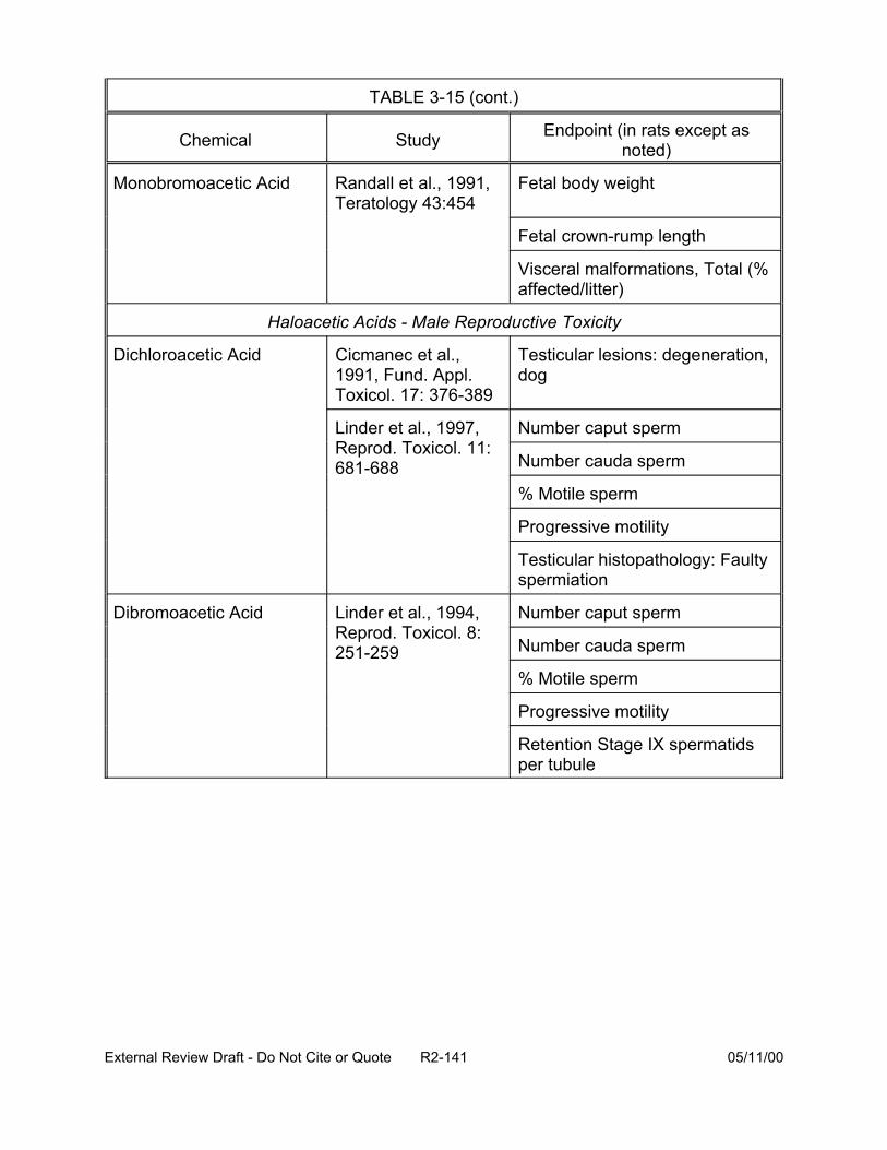
TABLE 3-15 (cont.)
Chemical Study Endpoint (in rats except as noted)
Monobromoacetic Acid Randall et al., 1991, Teratology 43:454
Fetal body weight
Fetal crown-rump length
Visceral malformations, Total (% affected/litter)
Haloacetic Acids - Male Reproductive Toxicity
Dichloroacetic Acid Cicmanec et al., 1991, Fund. Appl. Toxicol. 17: 376-389
Testicular lesions: degeneration, dog
Linder et al., 1997, Reprod. Toxicol. 11: 681-688
Number caput sperm
Number cauda sperm
% Motile sperm
Progressive motility
Testicular histopathology: Faulty spermiation
Dibromoacetic Acid Linder et al., 1994, Reprod. Toxicol. 8: 251-259
Number caput sperm
Number cauda sperm
% Motile sperm
Progressive motility
Retention Stage IX spermatids per tubule
External Review Draft - Do Not Cite or Quote R2-141 05/11/00
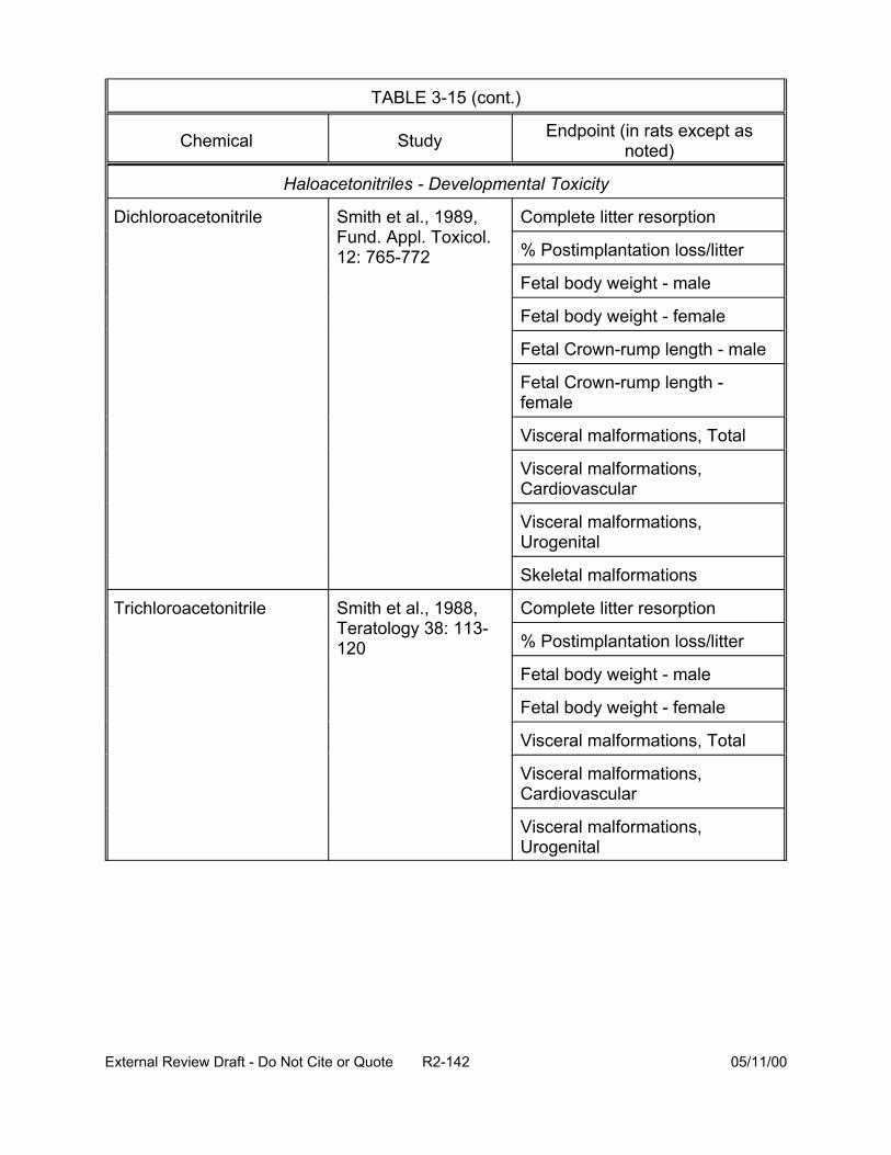
TABLE 3-15 (cont.)
Chemical Study Endpoint (in rats except as noted)
Haloacetonitriles - Developmental Toxicity
Dichloroacetonitrile Smith et al., 1989, Fund. Appl. Toxicol. 12: 765-772
Complete litter resorption
% Postimplantation loss/litter
Fetal body weight - male
Fetal body weight - female
Fetal Crown-rump length - male
Fetal Crown-rump length -female
Visceral malformations, Total
Visceral malformations, Cardiovascular
Visceral malformations, Urogenital
Skeletal malformations
Trichloroacetonitrile Smith et al., 1988, Teratology 38: 113-120
Complete litter resorption
% Postimplantation loss/litter
Fetal body weight - male
Fetal body weight - female
Visceral malformations, Total
Visceral malformations, Cardiovascular
Visceral malformations, Urogenital
External Review Draft - Do Not Cite or Quote R2-142 05/11/00
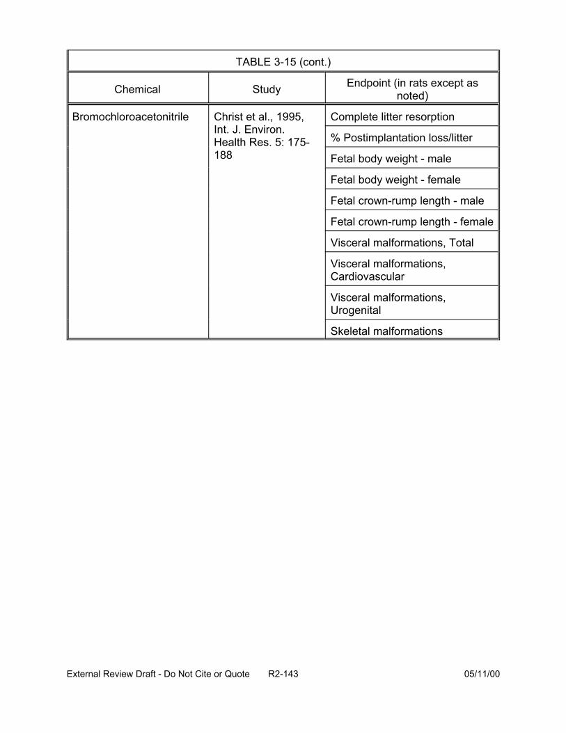
TABLE 3-15 (cont.)
Chemical Study Endpoint (in rats except as noted)
Bromochloroacetonitrile Christ et al., 1995, Int. J. Environ.
Complete litter resorption
Health Res. 5: 175-188
% Postimplantation loss/litter
Fetal body weight - male
Fetal body weight - female
Fetal crown-rump length - male
Fetal crown-rump length - female
Visceral malformations, Total
Visceral malformations, Cardiovascular
Visceral malformations, Urogenital
Skeletal malformations
External Review Draft - Do Not Cite or Quote R2-143 05/11/00
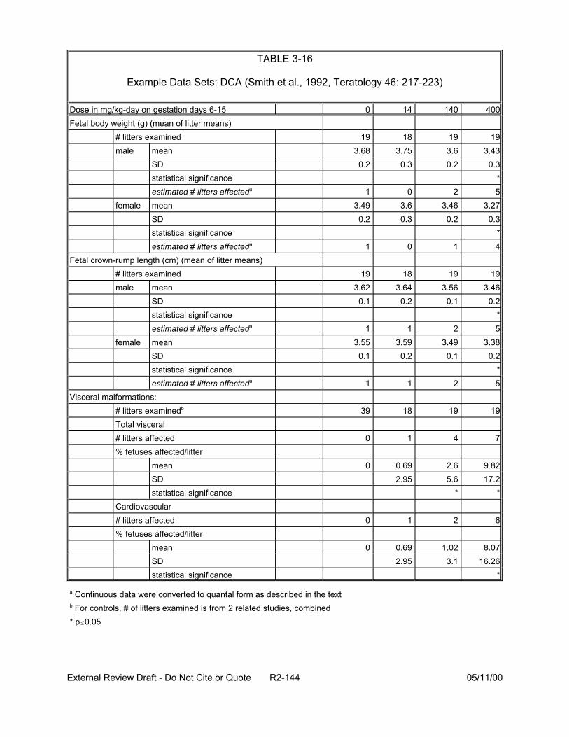
TABLE 3-16
Example Data Sets: DCA (Smith et al., 1992, Teratology 46: 217-223)
Dose in mg/kg-day on gestation days 6-15 0 14 140 400 Fetal body weight (g) (mean of litter means)
# litters examined 19 18 19 male mean 3.68 3.75 3.6
SD 0.2 0.3 0.2 statistical significance estimated # litters affecteda 1 2
female mean 3.49 3.6 3.46 SD 0.2 0.3 0.2 statistical significance estimated # litters affecteda 1 1
Fetal crown-rump length (cm) (mean of litter means) # litters examined 19 18 19 male mean 3.62 3.64 3.56
SD 0.1 0.2 0.1 statistical significance estimated # litters affecteda 1 2
female mean 3.55 3.59 3.49 SD 0.1 0.2 0.1 statistical significance estimated # litters affecteda 1 2
Visceral malformations: # litters examinedb 39 18 19 Total visceral # litters affected 0 1 4 % fetuses affected/litter
mean 0 0.69 2.6 SD 2.95 5.6 statistical significance *
Cardiovascular # litters affected 0 1 2 % fetuses affected/litter
mean 0 0.69 1.02 SD 2.95 3.1 statistical significance *
0
0
1
1
19 3.43
0.3 *
3.27 0.3
*
19 3.46
0.2 *
3.38 0.2
*
19
7
9.82 17.2
*
6
8.07 16.26
5
4
5
5
a Continuous data were converted to quantal form as described in the text b For controls, # of litters examined is from 2 related studies, combined * p#0.05
External Review Draft - Do Not Cite or Quote R2-144 05/11/00
are quantal, but other data (body weight, crown-rump length) are continuous, and were
converted to quantal (estimated # of litters affected in the table) prior to modeling.
Conversion of the continuous-response developmental data to quantal form was
performed by assuming a normal distribution with a constant variance across dose
groups for the response, and 5% background response rate. Because individual animal
data were not available, the number of responders in each dose group was estimated
by first establishing a critical value representing the point above (or below, depending
on the direction of adverse response) which 5% of the control group lies. Then, for
each dose group, the proportion exceeding this critical value was estimated. This
proportion was applied to the number of animals in the dose group to determine the
number of responders. The doses were converted to equivalent human doses using the
scaling factor of body weight to the 3/4 power. A threshold dose-response model was
then fit to the data sets for the individual DBP.
As shown previously in Table 3-15, adequate developmental toxicity data were
lacking for the haloacetic acids DBA and BCA and for the haloacetonitriles DBAN and
DBCAN. A surrogate approach seemed appropriate to fill these data gaps, because the
available data indicated that developmental toxicity may be common to the haloacetic
acid and haloacetonitrile DBP. As a provisional measure, DCA was selected as a
surrogate for these haloacetic acids and TCAN was selected as a surrogate for these
haloacetonitriles. A search for mechanistic data to support selection of surrogates
revealed studies of mechanisms relevant to carcinogenicity, which may not be relevant
to developmental toxicity, and some in vitro embryo culture studies, which did not
appear to give results corresponding to the available in vivo testing. Therefore the
External Review Draft - Do Not Cite or Quote R2-145 05/11/00
selections of surrogates were based partly on structural similarity and partly on quality
of the data (such as better dose spacing) for the surrogate.
The proportional response additivity approach was applied to concentration data
from two pilot studies of drinking water disinfection processes: one using Mississippi
River water at Jefferson Parish, LA (Lykins et al., 1991) and the other using Ohio River
water (Miltner et al., 1990; with further analysis by NCEA-CIN EPA). Data sets for water
treated with chlorine were chosen because this process results in higher levels of the
haloacetic acids and haloacetonitriles relative to other methods, such as pretreatment
with ozone prior to disinfection with chlorine, and/or other disinfectants such as
chloramine.
3.8.3. Results. Risks of developmental toxicity were estimated for humans ingesting
drinking water containing the haloacetic acids and haloacetonitriles at the
concentrations determined in the pilot studies described in the previous section. The
risk estimates were based on increased total visceral malformations, increased
cardiovascular malformations, decreased fetal body weight, and decreased fetal crown-
rump length. [Because the reports of the animal data for MCA and MBA did not break
out the cardiovascular incidence data from the total visceral malformation data (stated
to be mainly cardiovascular), the proportional risk estimates for cardiovascular
malformations used total visceral malformations for those two chemicals.] The risk
estimates were similar for total visceral malformations, cardiovascular malformations,
and decreased fetal weight, and somewhat lower for decreased fetal crown-rump
length.
External Review Draft - Do Not Cite or Quote R2-146 05/11/00
The risk estimates based on total visceral malformations were selected to
illustrate the application of proportional response additivity, because these estimates
best illustrated the use of surrogates. Details of these estimates are provided in Tables
3-17 and 3-18. The concentration data, in :g/L, were converted to human doses by
assuming water consumption of 2 L/day and a body weight of 70 kg. The total
combined dose of haloacetic acids and haloacetonitriles was approximately 4 :g/kg-day
for Jefferson Parish (Mississippi River) water and 2 :g/kg-day for the Ohio River water.
The risk for each DBP was estimated at the total mixture dose (as if the DBP were
present at a dose equal to the whole mixture dose) using a threshold dose response
model as previously described. The risk for some components was zero because the
threshold for these components was higher than the total mixture dose. The
proportional risk for each component was then calculated by multiplying risk at the total
mixture dose by the proportion of that component in the mixture. The sum of the
proportional risks, or total risk, for the two sets of drinking water data was 1.2 x 10⁻⁵ for
Jefferson Parish/Mississippi River and 8.9 x 10⁻⁶ for the Ohio River. These values are
virtually identical, and indicate a relatively low risk for developmental toxicity (.1 in
100,000) during the gestational period.
If proportional risks based on surrogates were omitted, the total risks for the two
sets of drinking water data were slightly lower: 7.4 x 10⁻⁶ and 7.1 x 10⁻⁶ (0.7 in 100,000).
Elimination of surrogates from the risk estimates had a similar impact for estimates
based on cardiovascular malformations, but virtually no impact on the estimates based
on fetal body weight and none on crown-rump length. Risk was also estimated for an
alternative disinfection method involving pretreatment of Ohio River water with ozone
External Review Draft - Do Not Cite or Quote R2-147 05/11/00

TABLE 3-17
Example Risk Estimate for Developmental Toxicity in Humans Exposed to Haloacetic Acids and Haloacetonitriles in Drinking Water at Concentrations Determined in Pilot Study, Jefferson Parish (Mississippi River) Following Chlorine
Treatment
Chemical Water Concentration :g/L
Estimated Dose
mg/kg-day
Proportion of Component in Mixture
Risk at Total Mixture Dosea
Proportional Riska
MCA 16 4.57E-04 11.93% 0 0
DCA 44.9 1.28E-03 33.48% 2.04E-05 6.8E-06
TCA 39.8 1.14E-03 29.68% 0 0
M BA 1.2 3.43E-05 0.89% 0 0
DBAb 0.8 2.29E-05 0.60% 2.04E-05 1.2E-07
BCAb 28.7 8.20E-04 21.40% 2.04E-05 4.4E-06
DCAN 1.6 4.57E-05 1.19% 0 0
TCAN 0.1 2.86E-06 0.07% 1.32E-04 9.8E-08
BCAN 0.7 2.00E-05 0.52% 1.01E-04 5.3E-07
DBAN Not listed — — — —
DBCANc 0.3 8.57E-06 0.22% 1.32E-04 2.9E-07
Sum — 3.83E-03 100.00% — 1.2E-05
a Based on dose-response data for total visceral malformations, using threshold dose-response modelb Estimated using the surrogate DCAc Estimated using the surrogate TCAN
External Review Draft - Do Not Cite or Quote R2-148 05/11/00
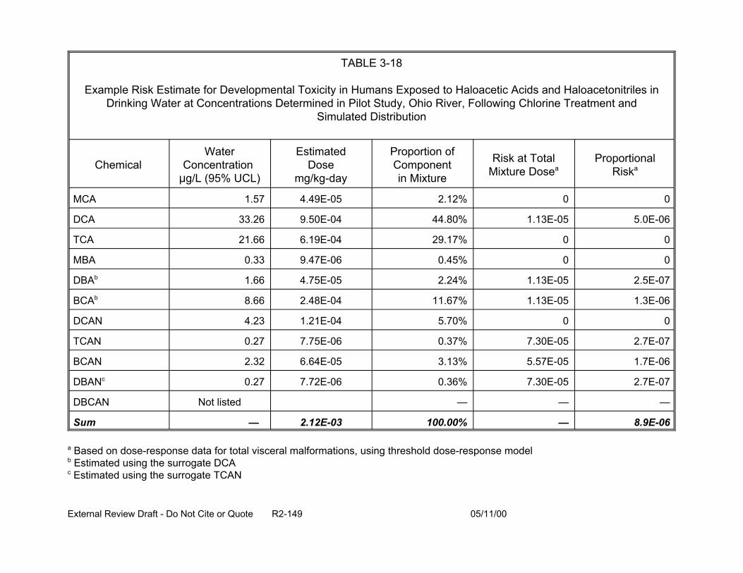
TABLE 3-18
Example Risk Estimate for Developmental Toxicity in Humans Exposed to Haloacetic Acids and Haloacetonitriles in Drinking Water at Concentrations Determined in Pilot Study, Ohio River, Following Chlorine Treatment and
Simulated Distribution
Chemical Water
Concentration :g/L (95% UCL)
Estimated Dose
mg/kg-day
Proportion of Component in Mixture
Risk at Total Mixture Dosea
Proportional Riska
MCA 1.57 4.49E-05 2.12% 0 0
DCA 33.26 9.50E-04 44.80% 1.13E-05 5.0E-06
TCA 21.66 6.19E-04 29.17% 0 0
MBA 0.33 9.47E-06 0.45% 0 0
DBAb 1.66 4.75E-05 2.24% 1.13E-05 2.5E-07
BCAb 8.66 2.48E-04 11.67% 1.13E-05 1.3E-06
DCAN 4.23 1.21E-04 5.70% 0 0
TCAN 0.27 7.75E-06 0.37% 7.30E-05 2.7E-07
BCAN 2.32 6.64E-05 3.13% 5.57E-05 1.7E-06
DBANc 0.27 7.72E-06 0.36% 7.30E-05 2.7E-07
DBCAN Not listed — — —
Sum — 2.12E-03 100.00% — 8.9E-06
a Based on dose-response data for total visceral malformations, using threshold dose-response modelb Estimated using the surrogate DCAc Estimated using the surrogate TCAN
External Review Draft - Do Not Cite or Quote R2-149 05/11/00

followed by chlorine. This treatment produced lower concentrations of most of the
haloacetic acids and haloacetonitriles, and lower total doses, but slightly higher
concentrations of MCA, DBA, BCAN, and DBAN than did the parallel disinfection
without ozone in the same pilot study. The estimated risk of developmental toxicity
(based on dose-response for total visceral malformations) for the alternative ozone-
chlorine treatment was 6.7 x 10⁻⁶, slightly lower than that for the chlorine treatment
shown in Table 3-18.
3.8.4. Future Directions. Several toxicological (biological and statistical) issues were
raised during this exercise that will require further analysis. These issues include: the
effect of the vehicle, tricaprylin, in the haloacetonitrile studies; the relevance of using the
gavage studies for extrapolation to the drinking water exposure scenario; the
appropriateness of combining data within a category (such as fetal size—fetal body
weight and crown-rump length); and the usefulness and relevance of in vitro studies
such as whole embryo culture for chemicals with inadequate in vivo data.
Further analysis of dose-response assessment of individual fetal data and of
male reproductive data for the haloacetic acids and haloacetonitriles may prove fruitful
for application of this method. In depth consideration of surrogate chemicals, including
pharmacokinetic and pharmacodynamic mechanisms warrants additional attention.
Another direction for future statistical efforts includes the exploration of alternative
methods for converting continuous response data and the feasibility of applying
proportional response addition across all of the mixture components for a continuous
endpoint prior to estimating the risk for the mixture.
External Review Draft - Do Not Cite or Quote R2-150 05/11/00
3.9. PRESENTATION: NEW MIXTURES METHODOLOGIES: RELATIVE POTENCY FACTORS, TOXIC EQUIVALENCY FACTORS WITH RESPONSE ADDITION (R. Hertzberg)
NCEA-Cin has been working on approaches for assessing the toxicity of classes
of similar chemicals. These approaches have included the Relative Potency Factor
(RPF) method, interactions hazard index, and extension of the RPF to more complex
mixtures.
3.9.1. Relative Potency Factors. Use of Toxicity Equivalency Factors (TEF), such as
those for dioxins, are the true form of dose-addition wherein the same mechanism of
action is assumed. There is one relative potency value per congener and the mixture
dose is treated as an equivalent dose of the index congener. Similar structure, the
same mechanism for toxicity, and data from several measures of toxicity are needed to
show that the relative potency of the congeners are constant across all effects, time
frames, species, routes, and assays. Often, there are insufficient data to validate a TEF
approach and few groups of chemicals qualify for its use. Therefore, in many site
assessments for classes of chemicals with data considered inadequate for TEF
development, either zero is assumed as a risk value for a congener with little toxicity
data or the toxicity of the most toxic congener is substituted.
Another approach, more general than the TEF approach, but requiring less
information and with more restricted application, is the RPF method (Table 3-19). The
TEF can be thought of as a specific type of RPF. The RPF approach also assumes
dose addition, requires similar structure or toxicity and empirical similarity amongst the
chemical class, but can be applied when such information only exists for organ-specific
External Review Draft - Do Not Cite or Quote R2-151 05/11/00
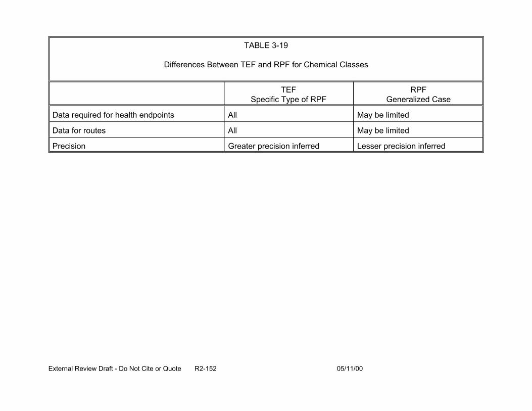
TABLE 3-19
Differences Between TEF and RPF for Chemical Classes
TEF Specific Type of RPF
RPF Generalized Case
Data required for health endpoints All May be limited
Data for routes All May be limited
Precision Greater precision inferred Lesser precision inferred
External Review Draft - Do Not Cite or Quote R2-152 05/11/00
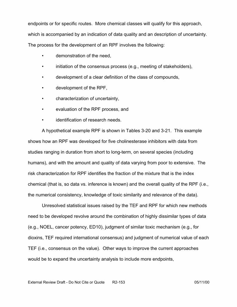
endpoints or for specific routes. More chemical classes will qualify for this approach,
which is accompanied by an indication of data quality and an description of uncertainty.
The process for the development of an RPF involves the following:
• demonstration of the need,
• initiation of the consensus process (e.g., meeting of stakeholders),
• development of a clear definition of the class of compounds,
• development of the RPF,
• characterization of uncertainty,
• evaluation of the RPF process, and
• identification of research needs.
A hypothetical example RPF is shown in Tables 3-20 and 3-21. This example
shows how an RPF was developed for five cholinesterase inhibitors with data from
studies ranging in duration from short to long-term, on several species (including
humans), and with the amount and quality of data varying from poor to extensive. The
risk characterization for RPF identifies the fraction of the mixture that is the index
chemical (that is, so data vs. inference is known) and the overall quality of the RPF (i.e.,
the numerical consistency, knowledge of toxic similarity and relevance of the data).
Unresolved statistical issues raised by the TEF and RPF for which new methods
need to be developed revolve around the combination of highly dissimilar types of data
(e.g., NOEL, cancer potency, ED10), judgment of similar toxic mechanism (e.g., for
dioxins, TEF required international consensus) and judgment of numerical value of each
TEF (i.e., consensus on the value). Other ways to improve the current approaches
would be to expand the uncertainty analysis to include more endpoints,
External Review Draft - Do Not Cite or Quote R2-153 05/11/00
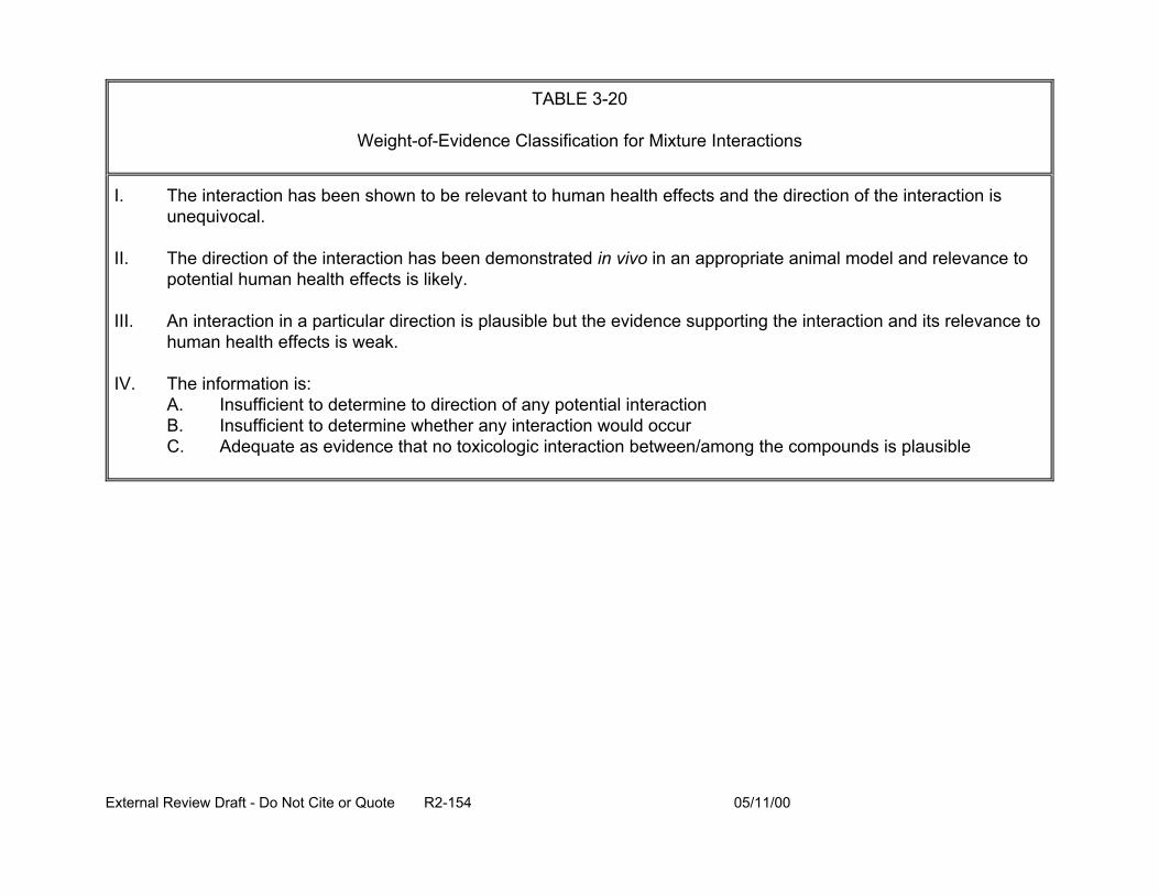
TABLE 3-20
Weight-of-Evidence Classification for Mixture Interactions
I. The interaction has been shown to be relevant to human health effects and the direction of the interaction is unequivocal.
II. The direction of the interaction has been demonstrated in vivo in an appropriate animal model and relevance to potential human health effects is likely.
III. An interaction in a particular direction is plausible but the evidence supporting the interaction and its relevance to human health effects is weak.
IV. The information is: A. Insufficient to determine to direction of any potential interaction B. Insufficient to determine whether any interaction would occur C. Adequate as evidence that no toxicologic interaction between/among the compounds is plausible
External Review Draft - Do Not Cite or Quote R2-154 05/11/00
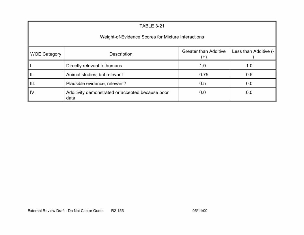
TABLE 3-21
Weight-of-Evidence Scores for Mixture Interactions
WOE Category Description Greater than Additive (+)
Less than Additive (-)
I. Directly relevant to humans 1.0 1.0
II. Animal studies, but relevant 0.75
III. Plausible evidence, relevant? 0.5
0.5
0.0
IV. Additivity demonstrated or accepted because poor data
0.0 0.0
External Review Draft - Do Not Cite or Quote R2-155 05/11/00
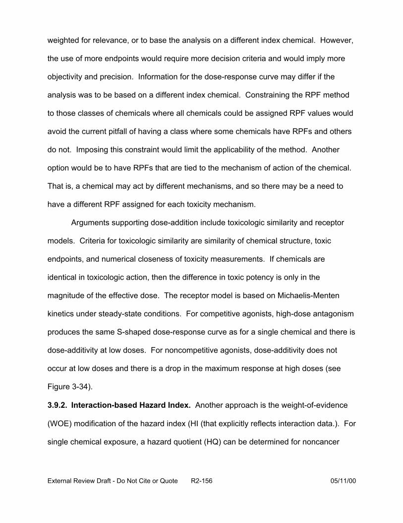
weighted for relevance, or to base the analysis on a different index chemical. However,
the use of more endpoints would require more decision criteria and would imply more
objectivity and precision. Information for the dose-response curve may differ if the
analysis was to be based on a different index chemical. Constraining the RPF method
to those classes of chemicals where all chemicals could be assigned RPF values would
avoid the current pitfall of having a class where some chemicals have RPFs and others
do not. Imposing this constraint would limit the applicability of the method. Another
option would be to have RPFs that are tied to the mechanism of action of the chemical.
That is, a chemical may act by different mechanisms, and so there may be a need to
have a different RPF assigned for each toxicity mechanism.
Arguments supporting dose-addition include toxicologic similarity and receptor
models. Criteria for toxicologic similarity are similarity of chemical structure, toxic
endpoints, and numerical closeness of toxicity measurements. If chemicals are
identical in toxicologic action, then the difference in toxic potency is only in the
magnitude of the effective dose. The receptor model is based on Michaelis-Menten
kinetics under steady-state conditions. For competitive agonists, high-dose antagonism
produces the same S-shaped dose-response curve as for a single chemical and there is
dose-additivity at low doses. For noncompetitive agonists, dose-additivity does not
occur at low doses and there is a drop in the maximum response at high doses (see
Figure 3-34).
3.9.2. Interaction-based Hazard Index. Another approach is the weight-of-evidence
(WOE) modification of the hazard index (HI (that explicitly reflects interaction data.). For
single chemical exposure, a hazard quotient (HQ) can be determined for noncancer
External Review Draft - Do Not Cite or Quote R2-156 05/11/00
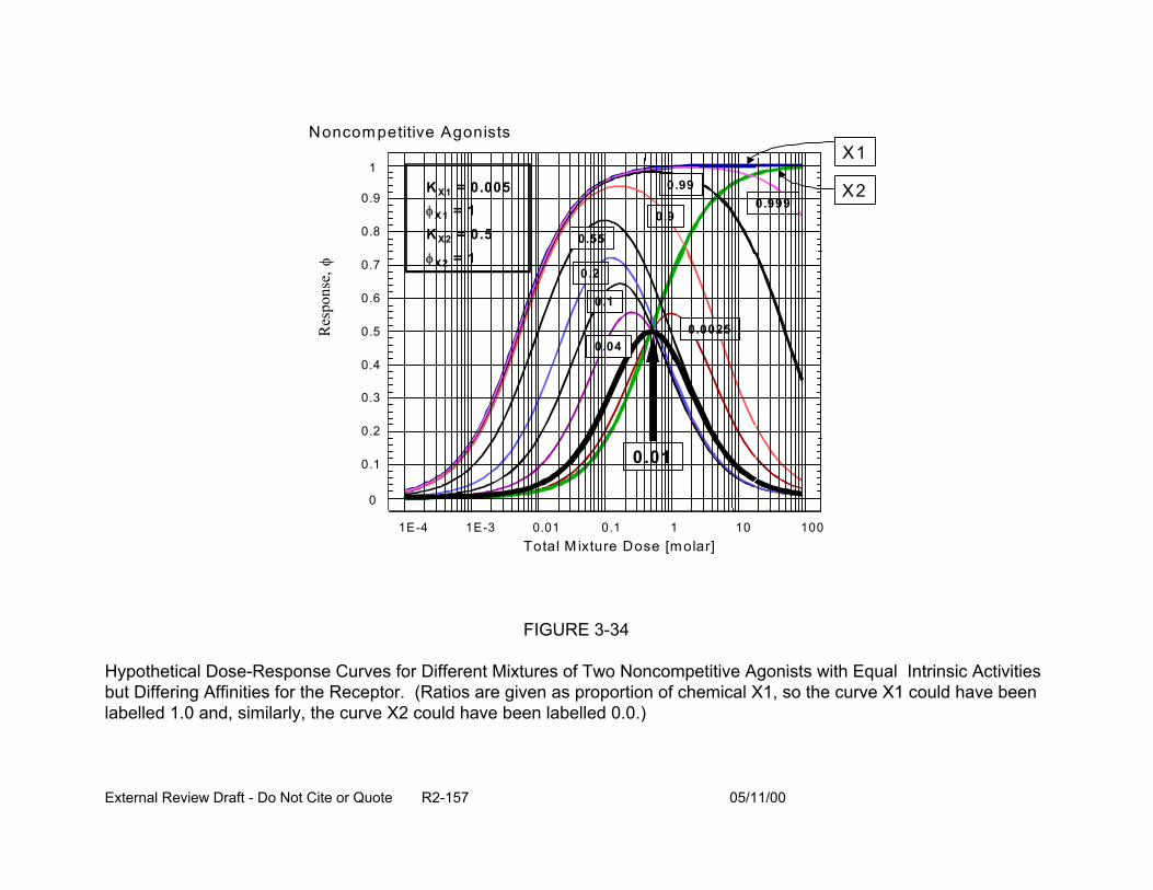
1
0.9
0.8
0.7
0.6
0.5
0.4
0.3
0.2
0.1
0
N oncom petitive A gonists X1
0.1
0.2
0.55
0.99
0.9 0.999
X2
0.0025 0.04
K X1 = 0.005 φ X1 = 1 K X2 = 0.5 φ X2 = 1
0.01
1E-4 1E-3 0.01 0.1 1 10 100 Total M ixture Dose [molar]
FIGURE 3-34
Hypothetical Dose-Response Curves for Different Mixtures of Two Noncompetitive Agonists with Equal Intrinsic Activities but Differing Affinities for the Receptor. (Ratios are given as proportion of chemical X1, so the curve X1 could have been labelled 1.0 and, similarly, the curve X2 could have been labelled 0.0.)
Res
pons
e, φ
External Review Draft - Do Not Cite or Quote R2-157 05/11/00
effects. The HQ, primarily used in Superfund risk assessments, indicates whether
intake of the chemical by a particular route (e.g., oral or inhalation) exceeds the
reference value (e.g., RfD or RfC) for that chemical for that route. The RfC or RfD is the
exposure value for a single chemical for which lifetime daily exposure is expected to be
associated with negligible risk of adverse effects, even in sensitive subgroups of the
exposed population. The HQ for a chemical for the oral route is:
EkHQk = RfDk
(3-13)
where:
E = exposure level (or intake)
RfD = oral reference dose
E and RfD are expressed in the same units (e.g., mg/kg-day) and represent the
same exposure period (e.g., chronic exposure).
For mixtures, noncancer effects are often assessed by estimating the HI (U.S.
EPA, 1986). The HI estimates whether combined exposure (or intake) of the
components exceeds the reference value for the mixture (which is the exposure-
weighted harmonic mean of reference values for each component). The HI is derived
from the concept of dose-addition and is generally calculated for a specific single toxic
effect (e.g., reproductive toxicity, hepatic toxicity), because dose-addition requires the
assumption of a similar mode of action (or toxicologic effect).
External Review Draft - Do Not Cite or Quote R2-158 05/11/00
The HI for a mixture of n chemicals is:
(3-14)
Exposure to the mixture is usually judged acceptable when the HI < 1. When HI
> 1, toxicity is deemed possible and further investigation is indicated. In practice,
separate HIs are determined for each toxic effect of interest, and acceptable exposure
is indicated whenever all HIs < 1.
The HI approach, however, does not take into consideration the toxicologic
interaction of components in the mixture. Existing data on toxicologic interactions are
primarily for binary mixtures (i.e., mixtures with two components). In general,
toxicologists assume that the magnitude of the interaction decreases with decreasing
dose, the magnitude is maximal when the component doses are equitoxic, and the
maximum change plausible in the toxicologic effective dose is a factor of about 10. As
currently used by EPA, data for the interaction of binary mixtures do not generally
change the outcome of the risk assessment, such as clean-up goals at Superfund sites,
unless there is strong evidence of a toxicologic interaction.
As a way to take into account interaction information in determining the HI,
Mumtaz and Durkin (1992) ranked toxicologic interaction information to estimate
confidence in the direction of the interaction (i.e., antagonism, additivity, synergism) and
converted that information into a weight-of-evidence (WOE) score. The WOE score
was used to convert the HI into an interaction HI (HIINT).
External Review Draft - Do Not Cite or Quote R2-159 05/11/00
Subsequent to the Mumtaz and Durkin (1992) approach, EPA developed a
slightly different approach (Hertzberg et al., 1999) whereby the HI can be modified to
account for interactions, as follows:
EkHQk = RfDk
(3-15)
Mjk is the estimate of the observed interaction magnitude, synergistic or
antagonistic, that chemical k has on the threshold or risk-specific dose (e.g., ED10) of
chemical j. The factor fjk, a function of the HQ values, is a normalizing or weighting
factor that is a rough measure of the relative toxicity of the kth component compared to
all the other chemicals that could interact with the jth chemical. The binary WOE factor,
Bjk, reflects the strength of studies showing that chemical k influences the toxicity of
chemical j and that the influence will be relevant to human health assessment. The
WOE classification on which B is based is similar to, but simpler than, the WOE process
of Mumtaz and Durkin (1992). It is dependent primarily on data quality factors and
relevance of the data to potential human health effects (Table 3-20); in most cases, this
related to the extent of any extrapolation. The WOE classification is converted into a
numerical weight; positive values indicate synergism and negative values indicate
antagonism (Table 3-21). For each pair of component chemicals in the mixture, two
WOEs are evaluated: first, for the influence on chemical j on the toxicity of chemical k,
and then for the influence of chemical k on the toxicity of chemical j. Factor gjk reflects
the degree to which components j and k are present in equitoxic amounts. In practice,
equitoxic chemicals are chemicals with equal HQs.
External Review Draft - Do Not Cite or Quote R2-160 05/11/00
The interaction HI incorporates the actual exposure levels of the components, the
estimated magnitude of each pairwise interaction, and the WOE scores. Thus, the
influences of all the other interacting chemicals are incorporated into each chemical’s
modified HQ. The modified HQs are then summed to get the interaction HI for the
mixture. For example, assume that there are three chemicals in a mixture, that pairwise
there is synergism, and that the observed interaction magnitude is 5 for each pair (M=
5). The HIINT for an equitoxic composition of 1:1:1 is 5 * HI (five times the standard
dose-additive HI), for a composition of 8:1:1 is 2.8 * HI, and for a composition of 98:1:1
is 1.4 *HI.
3.9.3. More Complex Mixtures. The Hazard Index and the Relative Potency Factors
procedures are applied to groups of toxicologically similar chemicals. A more
complicated situation usually occurs, where the exposure is to a collection of chemicals,
some that are toxicologically similar, some that interact, and some that are independent.
Such a mixture could be assessed by dividing it into separate groups, and then
combining the resulting assessments. For example, consider the mixture containing a
group (A) of similar chemicals and a group (B) of independent chemicals, where the
latter group is also toxicologically independent from the similarity group. First, RPFs are
applied to group A, the similarity group, so that group A’s exposure is represented by
the equivalent exposure to the index chemical (call it X). Second, response addition is
applied to the combination of the independent group’s exposure with the index
chemical’s equivalent exposure. The combined risk for these two exposures (group B
and the X equivalent) are combined as if they were two independent chemicals.
External Review Draft - Do Not Cite or Quote R2-161 05/11/00
A more difficult case is when the first group includes some interacting chemicals.
A proposed approach might be to characterize that group by the interaction-based HI.
The difficulty is that the HI is not a risk estimate and so cannot be directly combined with
a risk or response estimated by response addition. One alternative calculation would
replace the relative toxicity weighting coefficients (1/RfD in Equation 3-13) by the
inverse of the ED10. For similar chemicals where dose addition applies, the resulting HI
can be interpreted in a response context: when HI=1, the mixture is at its ED10.
Unfortunately, for other values of HI, and for interaction-based HI calculations, no
interpretation has yet been proposed in terms of estimated response or risk.
3.10. PRESENTATION: EXPERT JUDGMENT FOR ASSESSING RISK: TOXICOLOGY AND EPIDEMIOLOGY (G. Gray)
3.10.1. Overview of Expert Judgment in Risk Assessment. Expert judgment uses
the knowledge and views of experts to characterize the scientific state of knowledge. It
is not a quick and easy way to avoid collection of data or analysis. As stated by Morgan
and Henrion (1992), “When you need to know the value of an uncertain quantity and
limits of data or understanding make standard methods impossible, the remaining
option is to ask experts for their best professional judgment”. Expert judgment has a
long history in many fields including engineering, finance, medicine, and environmental
risk analysis. The field of decision analysis recognizes explicit expert judgment as a
legitimate means for characterizing uncertain model parameters with little or no directly
applicable data or that require the synthesis of several lines of evidence.
Eliciting expert judgment is a field with its own literature and standards of practice
(for general references see Cooke, 1991; Keeney and von Winterfeldt, 1989; Lindley,
1991; Otway and von Winterfeldt, 1992). It requires the analyst (the person trying to get
External Review Draft - Do Not Cite or Quote R2-162 05/11/00
the information from the experts) to understand the field, work with experts, and
document the expert judgments. There are two approaches to eliciting expert judgment:
direct elicitation and problem disaggregation and elicitation on individual parts. These
approaches may be used together as was the case in the chloroform project (Evans et
al., 1994b). Through these processes, expert judgment is made explicit, a quantitative
sense of uncertainty is provided, and key sources of uncertainty are identified. In
addition, areas of agreement and disagreement among scientists are highlighted,
helping to focus future research efforts. Expert judgment facilitates honest
communication with decision makers and the public.
Formulation of a protocol for elicitation of expert judgment requires several key
elements including:
• clear formulation of questions (clairvoyance test),
• experts must be encouraged to think of a full range of uncertainty,
• several types of expertise may be necessary for complex problems, and
• experts should be trained in calibration.
Who to choose as an expert and how to choose experts are important issues in
expert judgment (Graham et al., 1988). Often, experts have bias in their research areas
and policy goals, and differ in their breadth and depth of knowledge. Calibration is an
important element in that experts often seem to be overconfident on general knowledge
questions. However, there is some evidence that experts may be reasonably well-
calibrated in their field (Hawkins and Evans, 1989). It must be clear what informs expert
judgment as experts in a field often likely read the same or similar body of literature or
may have received the same training. The issue of independence of expert judgments
External Review Draft - Do Not Cite or Quote R2-163 05/11/00
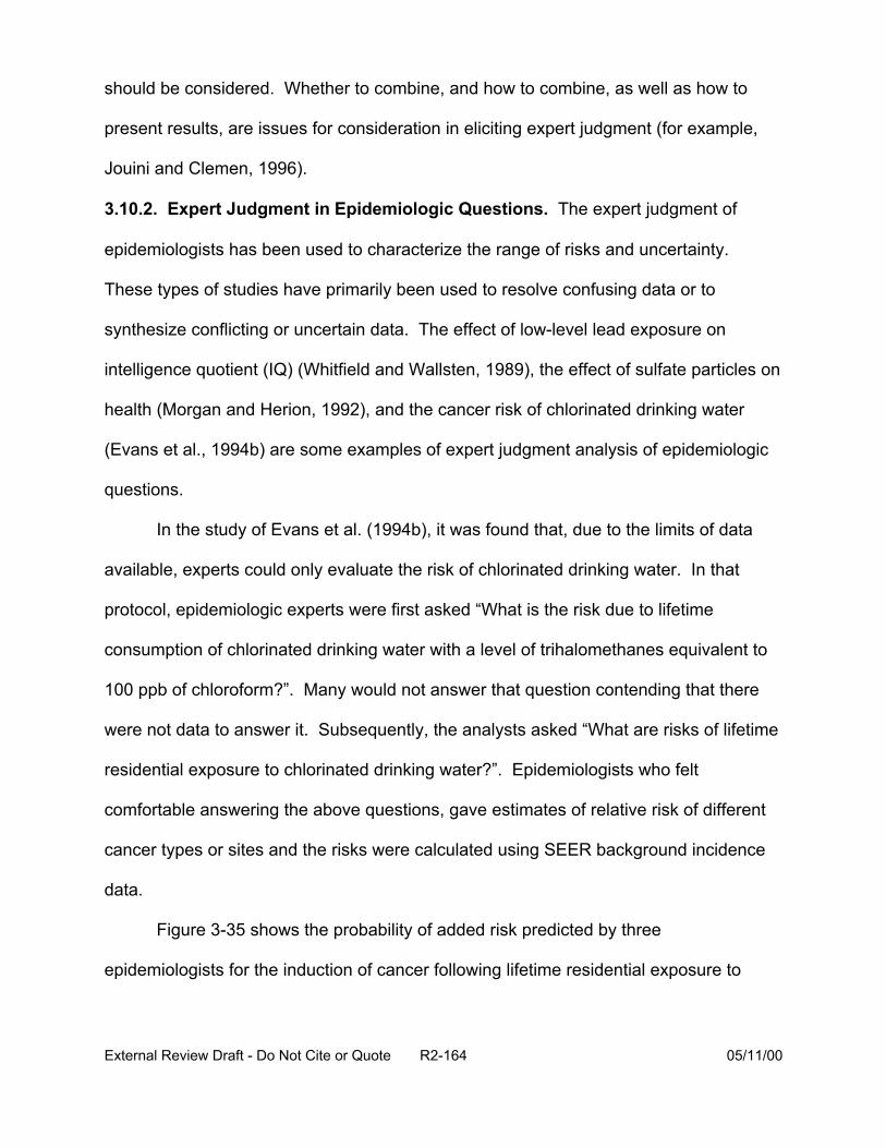
should be considered. Whether to combine, and how to combine, as well as how to
present results, are issues for consideration in eliciting expert judgment (for example,
Jouini and Clemen, 1996).
3.10.2. Expert Judgment in Epidemiologic Questions. The expert judgment of
epidemiologists has been used to characterize the range of risks and uncertainty.
These types of studies have primarily been used to resolve confusing data or to
synthesize conflicting or uncertain data. The effect of low-level lead exposure on
intelligence quotient (IQ) (Whitfield and Wallsten, 1989), the effect of sulfate particles on
health (Morgan and Herion, 1992), and the cancer risk of chlorinated drinking water
(Evans et al., 1994b) are some examples of expert judgment analysis of epidemiologic
questions.
In the study of Evans et al. (1994b), it was found that, due to the limits of data
available, experts could only evaluate the risk of chlorinated drinking water. In that
protocol, epidemiologic experts were first asked “What is the risk due to lifetime
consumption of chlorinated drinking water with a level of trihalomethanes equivalent to
100 ppb of chloroform?”. Many would not answer that question contending that there
were not data to answer it. Subsequently, the analysts asked “What are risks of lifetime
residential exposure to chlorinated drinking water?”. Epidemiologists who felt
comfortable answering the above questions, gave estimates of relative risk of different
cancer types or sites and the risks were calculated using SEER background incidence
data.
Figure 3-35 shows the probability of added risk predicted by three
epidemiologists for the induction of cancer following lifetime residential exposure to
External Review Draft - Do Not Cite or Quote R2-164 05/11/00
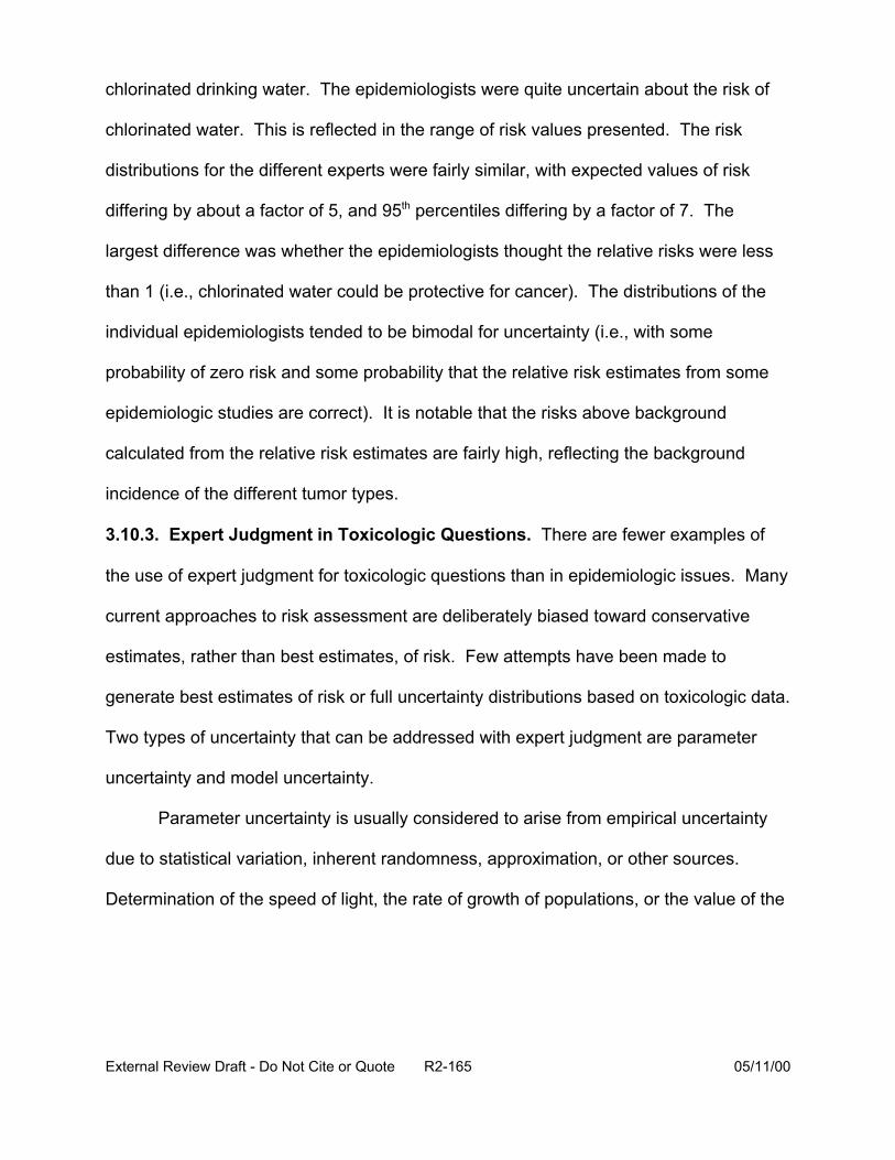
chlorinated drinking water. The epidemiologists were quite uncertain about the risk of
chlorinated water. This is reflected in the range of risk values presented. The risk
distributions for the different experts were fairly similar, with expected values of risk
differing by about a factor of 5, and 95th percentiles differing by a factor of 7. The
largest difference was whether the epidemiologists thought the relative risks were less
than 1 (i.e., chlorinated water could be protective for cancer). The distributions of the
individual epidemiologists tended to be bimodal for uncertainty (i.e., with some
probability of zero risk and some probability that the relative risk estimates from some
epidemiologic studies are correct). It is notable that the risks above background
calculated from the relative risk estimates are fairly high, reflecting the background
incidence of the different tumor types.
3.10.3. Expert Judgment in Toxicologic Questions. There are fewer examples of
the use of expert judgment for toxicologic questions than in epidemiologic issues. Many
current approaches to risk assessment are deliberately biased toward conservative
estimates, rather than best estimates, of risk. Few attempts have been made to
generate best estimates of risk or full uncertainty distributions based on toxicologic data.
Two types of uncertainty that can be addressed with expert judgment are parameter
uncertainty and model uncertainty.
Parameter uncertainty is usually considered to arise from empirical uncertainty
due to statistical variation, inherent randomness, approximation, or other sources.
Determination of the speed of light, the rate of growth of populations, or the value of the
External Review Draft - Do Not Cite or Quote R2-165 05/11/00
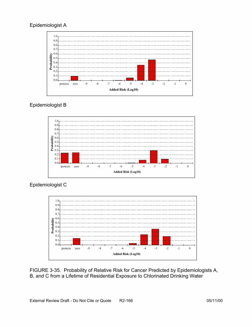
External Review Draft - Do Not Cite or Quote R2-166 05/11/00
0.00.10.20.30.40.50.60.70.80.91.0
protects zero -9 8 7 -6 5 4 -3 2 -1 0
Added Risk (Log10)
Prob
abili
ty
0.00.10.20.30.40.50.60.70.80.91.0
protects zero -9 -8 -7 -6 -5 -4 -3 -2 -1 0
Added Risk (Log10)
Prob
abili
ty
0.00.10.20.30.40.50.60.70.80.91.0
protects zero -9 8 -7 -6 -5 4 -3 2 1 0
Added Risk (Log10)
Prob
abili
ty
Epidemiologist A
Epidemiologist B
Epidemiologist C
FIGURE 3-35. for Cancer Predicted by Epidemiologists A,B, and C from a Lifetime of Residential Exposure to Chlorinated Drinking Water
- - - - -
- - - -
Probability of Relative Risk
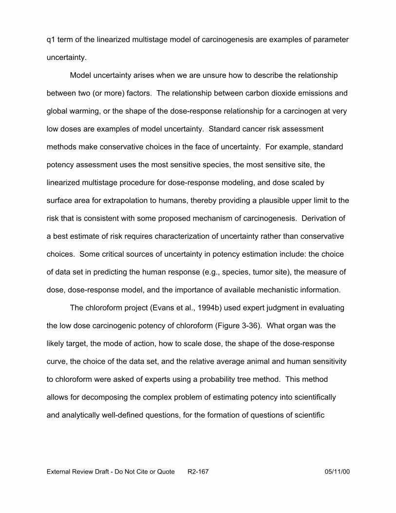
q1 term of the linearized multistage model of carcinogenesis are examples of parameter
uncertainty.
Model uncertainty arises when we are unsure how to describe the relationship
between two (or more) factors. The relationship between carbon dioxide emissions and
global warming, or the shape of the dose-response relationship for a carcinogen at very
low doses are examples of model uncertainty. Standard cancer risk assessment
methods make conservative choices in the face of uncertainty. For example, standard
potency assessment uses the most sensitive species, the most sensitive site, the
linearized multistage procedure for dose-response modeling, and dose scaled by
surface area for extrapolation to humans, thereby providing a plausible upper limit to the
risk that is consistent with some proposed mechanism of carcinogenesis. Derivation of
a best estimate of risk requires characterization of uncertainty rather than conservative
choices. Some critical sources of uncertainty in potency estimation include: the choice
of data set in predicting the human response (e.g., species, tumor site), the measure of
dose, dose-response model, and the importance of available mechanistic information.
The chloroform project (Evans et al., 1994b) used expert judgment in evaluating
the low dose carcinogenic potency of chloroform (Figure 3-36). What organ was the
likely target, the mode of action, how to scale dose, the shape of the dose-response
curve, the choice of the data set, and the relative average animal and human sensitivity
to chloroform were asked of experts using a probability tree method. This method
allows for decomposing the complex problem of estimating potency into scientifically
and analytically well-defined questions, for the formation of questions of scientific
External Review Draft - Do Not Cite or Quote R2-167 05/11/00
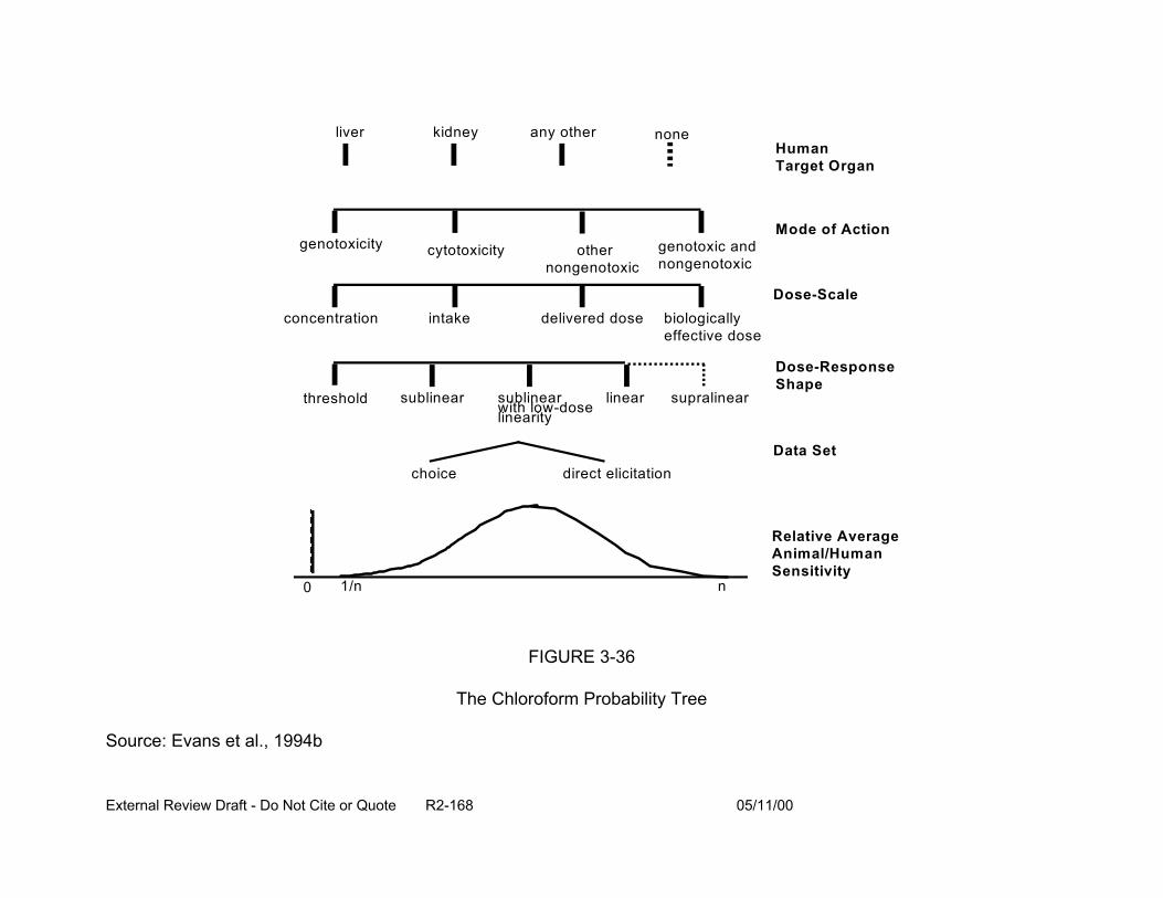
liver kidney any other none Human Target Organ
Mode of Action genotoxicity cytotoxicity other genotoxic and
nongenotoxic nongenotoxic
Dose-Scale delivered dose biologically
effective dose concentration intake
threshold sublinear sublinear with low-dose
linear supralinear linearity
Dose-Response Shape
Data Set
Relative Average Animal/Human Sensitivity
choice
0 1/n
direct elicitation
n
FIGURE 3-36
The Chloroform Probability Tree
Source: Evans et al., 1994b
External Review Draft - Do Not Cite or Quote R2-168 05/11/00
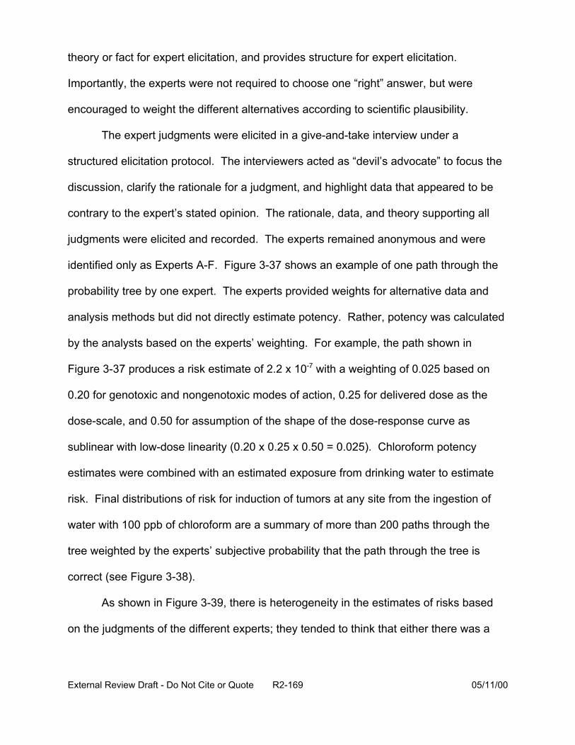
theory or fact for expert elicitation, and provides structure for expert elicitation.
Importantly, the experts were not required to choose one “right” answer, but were
encouraged to weight the different alternatives according to scientific plausibility.
The expert judgments were elicited in a give-and-take interview under a
structured elicitation protocol. The interviewers acted as “devil’s advocate” to focus the
discussion, clarify the rationale for a judgment, and highlight data that appeared to be
contrary to the expert’s stated opinion. The rationale, data, and theory supporting all
judgments were elicited and recorded. The experts remained anonymous and were
identified only as Experts A-F. Figure 3-37 shows an example of one path through the
probability tree by one expert. The experts provided weights for alternative data and
analysis methods but did not directly estimate potency. Rather, potency was calculated
by the analysts based on the experts’ weighting. For example, the path shown in
Figure 3-37 produces a risk estimate of 2.2 x 10⁻⁷ with a weighting of 0.025 based on
0.20 for genotoxic and nongenotoxic modes of action, 0.25 for delivered dose as the
dose-scale, and 0.50 for assumption of the shape of the dose-response curve as
sublinear with low-dose linearity (0.20 x 0.25 x 0.50 = 0.025). Chloroform potency
estimates were combined with an estimated exposure from drinking water to estimate
risk. Final distributions of risk for induction of tumors at any site from the ingestion of
water with 100 ppb of chloroform are a summary of more than 200 paths through the
tree weighted by the experts’ subjective probability that the path through the tree is
correct (see Figure 3-38).
As shown in Figure 3-39, there is heterogeneity in the estimates of risks based
on the judgments of the different experts; they tended to think that either there was a
External Review Draft - Do Not Cite or Quote R2-169 05/11/00
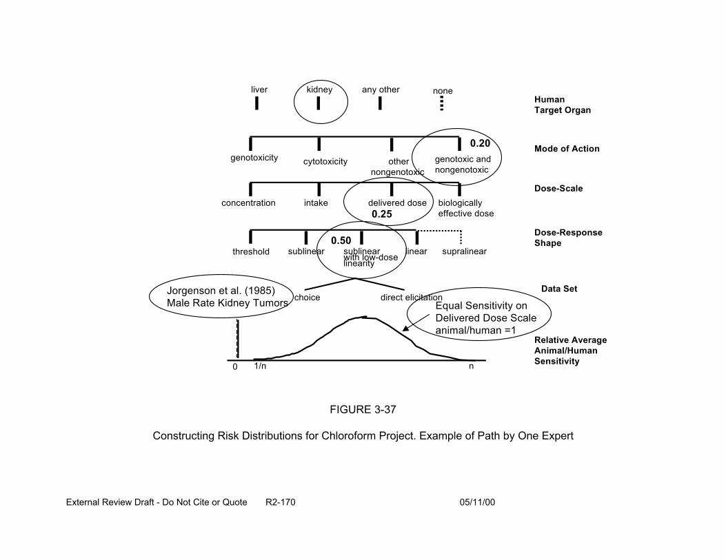
liver kidney any other none Human Target Organ
concentration intake delivered dose biologically effective dose
Dose-Scale
Dose-Response Shape
Data Set
genotoxicity genotoxic and nongenotoxic
Mode of Action other
nongenotoxic cytotoxicity
Relative Average Animal/Human Sensitivity
threshold supralinear
choice direct elicitation
sublinear sublinear with low-doselinearity
linear
0.20
0.25
0.50
Jorgenson et al. (1985) Male Rate Kidney Tumors Equal Sensitivity on
Delivered Dose Scale animal/human =1
0 1/n n
FIGURE 3-37
Constructing Risk Distributions for Chloroform Project. Example of Path by One Expert
External Review Draft - Do Not Cite or Quote R2-170 05/11/00
External Review Draft - Do Not Cite or Quote R2-171 05/11/00
Added Risk (Log10)
0.0
0.1
0.2
0.3
0.4
0.5
0.6
0.7
0.8
0.9
1.0
<-10 -9 -8 -7 -6 -5 -4 -3 -2 -1 0
A
Added Risk (Log10)
0.00.1
0.20.30.40.50.60.70.8
0.91.0
<-10 -9 -8 -7 -6 -5 -4 -3 -2 -1 0
B
Added Risk (Log10)
0.00.1
0.20.30.40.50.60.70.8
0.91.0
<-10 -9 -8 -7 -6 -5 -4 -3 -2 -1 0
C
Added Risk (Log10)
0.0
0.1
0.2
0.3
0.4
0.5
0.6
0.7
0.8
0.9
1.0
<-10 -9 -8 -7 -6 -5 -4 -3 -2 -1 0
D
Added Risk (Log10)
0.00.1
0.20.30.40.50.60.70.8
0.91.0
<-10 -9 -8 -7 -6 -5 -4 -3 -2 -1 0
E
Added Risk (Log10)
0.00.1
0.20.30.40.50.60.70.8
0.91.0
<-10 -9 -8 -7 -6 -5 -4 -3 -2 -1 0
F
FIGURE 3-38
Results for Individual Experts for 100 ppb Chloroform in Drinking Water Tumor Induction at Any Site
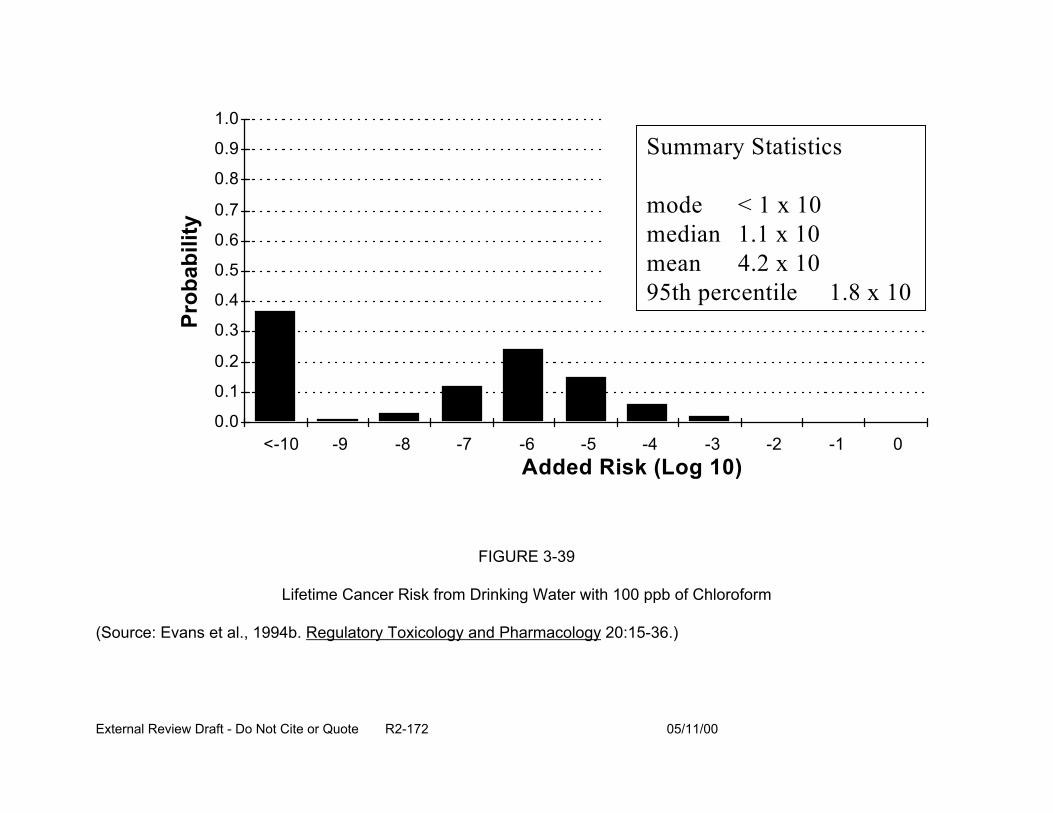
Prob
abili
ty
1.0
0.9
0.8
0.7
0.6
0.5
0.4
0.3
0.2
0.1
0.0
Summary Statistics
mode < 1 x 10 median 1.1 x 10 mean 2 x 10 95th percentile 1.8 x 10
4.
<-10 -9 -8 -7 -6 -5 -4 -3 -2 Added Risk (Log 10)
FIGURE 3-39
Lifetime Cancer Risk from Drinking Water with 100 ppb of Chloroform
(Source: Evans et al., 1994b. Regulatory Toxicology and Pharmacology 20:15-36.)
External Review Draft - Do Not Cite or Quote R2-172 05/11/00
-1 0
significant health risk for cancer from chloroform in drinking water or there was not.
There is considerable controversy about whether to combine expert judgments, and
how to do it if it is to be done (Clemen, 1989). As one means of combining estimates,
each expert was asked to weight their knowledge on each level of the tree. For
example, if an expert thought s/he was equally knowledgeable about all, then the
weights would be evenly distributed. The expert could indicate the different levels of
expertise with different weights. The trees and the “self-weighted” combined distribution
were then calculated; these are shown in Figure 3-40.
The chloroform project demonstrated that expert judgment can be used to
quantify model uncertainty in cancer potency estimation. The distributional approach
highlighted areas of agreement and disagreement among experts as well as
characterized uncertainty and allowed a better understanding of the likelihood of
alternative estimates of risk. In addition, the method allowed all relevant scientific
evidence about the carcinogenic potential of a chemical to be considered. Table 3-22
shows the strengths and weaknesses of the distributional approach in expert judgment.
3.10.4. Summary. Evaluating epidemiologic and toxicologic information through an
expert judgment analysis is no different than eliciting judgment from traditional sources.
However, ensuring that both analyses are addressing the same question (e.g.,
specificity of data, differences in confounding factors) and also uncertainty (e.g.,
overlapping uncertainty bounds) would be key concerns. For example, in the
chloroform project, toxicologists had data on the carcinogenicity (e.g., mechanism,
animal bioassay) of chloroform, whereas the epidemiologists reviewed data concerning
the differences in cancer rates between populations drinking chlorinated or non-
External Review Draft - Do Not Cite or Quote R2-173 05/11/00
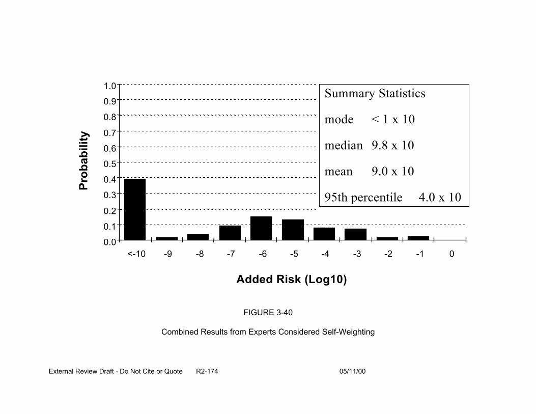
Prob
abili
ty
1.0
0.9
0.8
0.7
0.6
0.5
0.4
0.3
0.2
0.1
0.0 <-10 -9 -8 -7 -6 -5 -4 -3 -2 -1 0
Summary Statistics
mode < 1 x 10
median 9.8 x 10
mean 0 x 10
95th percentile 4.0 x 10
9.
Added Risk (Log10)
FIGURE 3-40
Combined Results from Experts Considered Self-Weighting
External Review Draft - Do Not Cite or Quote R2-174 05/11/00

TABLE 3-22
Distributional Approach to Expert Judgment
Weaknesses Strengths
• Relies on expert judgment which is • known to have several problems including “overconfidence” or lack • of willingness to answer questions
• Sensitive to choice of experts • Rewards advances in scientific knowledge
• Relative costly and analytically intensive
• Identifies key sources of uncertainty
• Highlights areas of agreement and disagreement among scientists -focus research efforts
• Facilitates honest communication with decision makers and the public
Makes expert judement explicit
Provides sense of uncertainty in estimates of potency
External Review Draft - Do Not Cite or Quote R2-175 05/11/00

chlorinated water. This meant that, ultimately, different questions were addressed by
the two groups of experts. The epidemiologists addressed the relative risk of
chlorinated water, while the toxicologists addressed the dose-response relationship of
chloroform for cancer. The distribution of risk from the epidemiologists was broad
enough so as not to be inconsistent with that of the toxicologists. However, the
differences in the distributions raise questions about the level of resolution based on the
data considered and the potential for protective effects of the water treatment.
Expert judgment has the potential to help analysis when data are sparse or
conflicting. Application of expert judgment must be aware of, and adhere to, norms of
the field. Differences in questions, data, and scale make it difficult to directly combine
the toxicologic and epidemiologic data. The use of expert judgment in policy-relevant
situations should increase its legitimacy. In the future, more attention is expected in the
field to combining issues across scientific disciplines, possibly using mechanistic data or
expert judgment as an aid in the combination.
3.11. PARTICIPANT DISCUSSION: IDENTIFICATION OF MAJOR ISSUES
Some participants noted that not all cancers are attributable to a heritable genetic
mutation, some are induced by epigenetic mechanisms. Cancer is more broadly
defined as a derangement or change in cell expression, growth, or death. Recent
literature suggests that mutations and other biological events are not random
occurrences. Under the proposed new cancer guidelines (U.S. EPA, 1996), EPA is
considering mode of action in their quantitative risk assessments (Section 4.3 provides
further discussion).
External Review Draft - Do Not Cite or Quote R2-176 05/11/00

The point was made that the developmental toxicity guidelines (U.S. EPA, 1991)
propose a threshold for developmental effects. Questions were raised about the
magnitude of intra-litter effects and whether it was appropriate to model individual
fetuses. The participants suggested that one way to get a handle on how big intra-litter
effects are, is to look at the same developmental toxicants in animals and humans. In
the majority of cases studies by Allen et al. (1994), litter size was an important
explanatory variable.
A question was raised as to why a log-logistic model was chosen for
developmental effects over a log-normal or probit model. As reported in Section 3.2, it
was found that the log-logistic model can describe the results from a wide variety of
actual, observed developmental toxicity studies. It was suggested that for the CRFM
case study, a benchmark dose (BMD), corresponding to 5% or 10% risk followed by use
of a toxicologically-based UF, could be likely be applied.
The participants made suggestions for human data sets such as thalidomide and
Vitamin A that could be examined for application of various dose-response modeling
approaches for developmental and reproductive data. Comparison/correlation of effects
in humans and animals could also been made using these data sets.
The ICR and water consumption analyses will fill in some significant gaps in
information for exposure assessment of the DBP (see Section 4.1 for more detailed
discussion). It was noted that there is a mini-ICR looking primarily at pathogen in
finished water.
It was noted that proportional response addition addresses the question of
unknowns in the mixture, and that 60-80% of the chemicals in drinking water are
External Review Draft - Do Not Cite or Quote R2-177 05/11/00
unknown. This approach can be applied with or without information as to mechanism or
mode of action and also in cases where dose-addition and response-addition are
applied.
The participants noted that the driver for calling chemicals similar or within the
same class (i.e., for TEF approaches) is based on a number of factors including
mechanism and chemical structure. The dioxin-like PCBs were pointed out as an
example. Pairwise data are needed to discern interactions of chemicals, very little of
which are available. NCEA-Cin reported that some work is currently being conducted
for interactions of chemicals at Superfund sites. In addition, NCEA and NHEERL are
conducting studies for pairs of trihalomethanes. One suggestion was to further develop
the cholinesterase example through additional testing of cholinesterase inhibitors. All of
these approaches are intended to be predictive; predictive approaches incorporate
QSAR. It was agreed that further research in this area is needed.
Publication bias in the epidemiologic literature was noted (i.e., negative studies
may not be published). This bias would affect the literature reviewed by the experts and
likely influence their judgment. The point was raised that epidemiologists may be
biased by their training toward a positive interpretation of findings to be protective of
public health (refer to Section 2.4 for additional discussion).
It was noted that all areas of a subject under question in an expert judgment
exercise need to be represented by a broad range of experts. For example, in the
discussion of chloroform carcinogenicity, general cancer experts as well as those
conducting research in a particular area need to be included. One participant thought
that the latter group may be biased towards their research perspective. To mitigate the
External Review Draft - Do Not Cite or Quote R2-178 05/11/00
potential for expert bias, analysts try to focus on specific scientific questions rather than
broad questions pertaining to risk or policy implications.
A suggestion was made that investigators using expert judgment look at the
responses of experts answering questions alone and also within a group (e.g., at a
workshop), as there may be differences in response related to input or presence of
peers. It was noted that anonymity of the experts may or may not affect the outcome. It
was suggested that obtaining the experts’ opinions prior to, as well as during a
workshop, might provide an indication of bias or the influence of peer presence. For
expert judgment to help resolve DBP risk, it was suggested that several mixture risk
assessments could conducted and experts queried as to how to weight the different
methods. Questions could be asked, that given the current state of the science, would
dose-addition, response-addition, proportional response addition or another way be the
most appropriate application for this mixture. Experts could also be queried about the
most appropriate health endpoint. Expert judgment will not resolve the problems of data
gaps or needed research, but may reconcile conflicting data.
External Review Draft - Do Not Cite or Quote R2-179 05/11/00
4. GROUP DISCUSSION
Seven discussion groups were formed to respond to the questions posed in the
workshop charge to the participants. The groups and their participants are shown in
Table 4-1. The following sections provide a summary of each breakout group’s
discussion. The participants were encouraged to think of these questions not just in the
context of the Comparative Risk Framework Methodology (CRFM), but more broadly in
how to approach risk assessment. These were:
1. Identify approaches that incorporate the observational and experimental data on disinfectant by-product (DBP) health effects (i.e., in vitro, in vivo and human data) into the risk assessment and still maintain the ability to compare risks across drinking water treatment options.
2. What techniques exist that can incorporate expert judgment into the risk estimates? For example, are there qualitative techniques that could be utilized to influence the process of developing quantitative estimates?
3. How can different aspects of the current approach to estimate the risks posed by DBP exposures be improved? Specifically, address the topics of concentration data, exposure estimates, dose-response information for both cancer and noncancer effects, use of Monte Carlo procedures, handling of uncertainty and variability, and the appropriateness of assumptions and endpoints used for mixtures risk estimation.
4. How should the toxicity of well-studies DBP, or of identified DBP, for which little or no data exist, be handled? Is it appropriate to use data on a similar chemical as surrogate data for another chemical?
5. For developmental, reproductive and non-genotoxic carcinogenicity, how can the concept of thresholds be handled? Is it reasonable to suggest that a mixtures toxicity threshold exists that is possibly well below the thresholds for the individual chemicals?
6. How should dose-response data from individual chemicals be combined and used in a mixtures risk assessment when their specific endpoints differ (e.g., both visceral malformations and crown rump length shortening to estimate developmental risks; or both liver and kidney tumors for cancer risk)?
External Review Draft - Do Not Cite or Quote R2-180 05/11/00
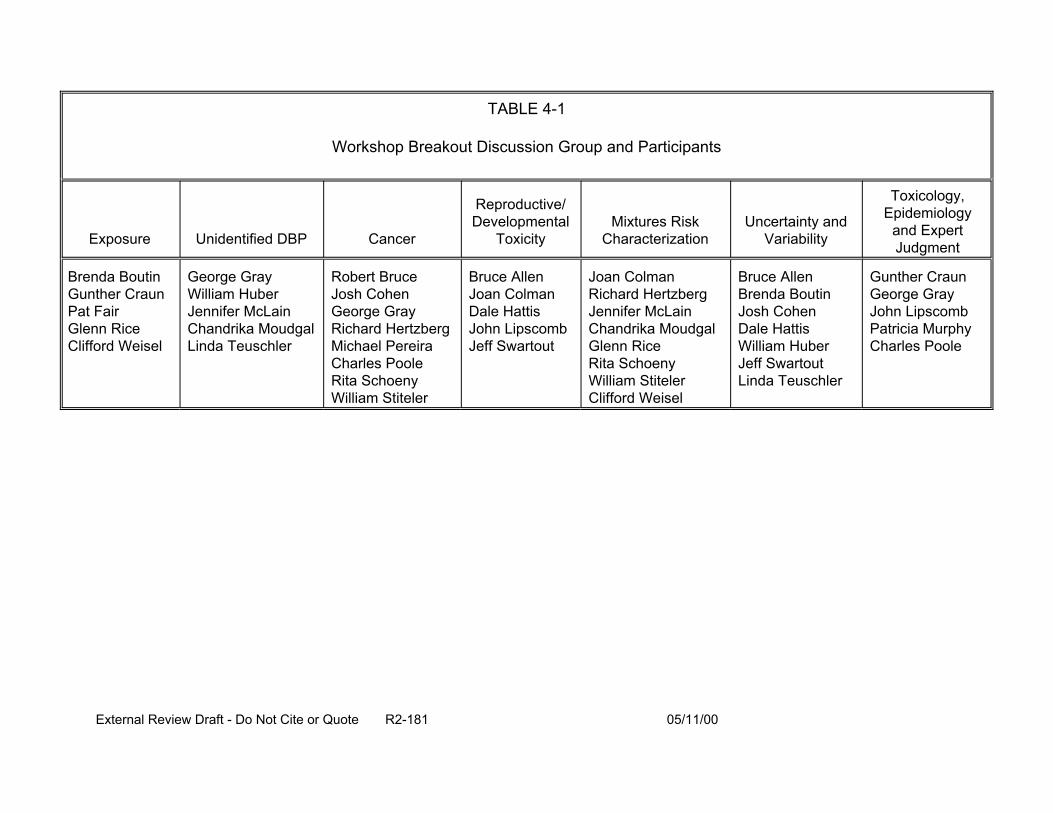
TABLE 4-1
Workshop Breakout Discussion Group and Participants
Exposure Unidentified DBP Cancer
Reproductive/ Developmental
Toxicity
Brenda Boutin Gunther Craun Pat Fair Glenn Rice Clifford Weisel
George Gray William Huber Jennifer McLain Chandrika Moudgal Linda Teuschler
Robert Bruce Josh Cohen George Gray Richard Hertzberg Michael Pereira Charles Poole Rita Schoeny William Stiteler
Bruce Allen Joan Colman Dale Hattis John Lipscomb Jeff Swartout
Mixtures Risk Characterization
Uncertainty and Variability
Toxicology, Epidemiology
and Expert Judgment
Joan Colman Richard Hertzberg Jennifer McLain Chandrika Moudgal Glenn Rice Rita Schoeny William Stiteler Clifford Weisel
Bruce Allen Brenda Boutin Josh Cohen Dale Hattis William Huber Jeff Swartout Linda Teuschler
Gunther Craun George Gray John Lipscomb Patricia Murphy Charles Poole
External Review Draft - Do Not Cite or Quote R2-181 05/11/00
7. Human cancer risks, largely based on animal data are interpreted by the EPA as “ the lifetime excess cancer risk per the exposure.” How should analogous developmental and reproductive risks be interpreted for the mixtures risk estimate?
8. Are there newer data and methods that EPA should be considering in order to improve these risk assessments? Specifically, address advancements in dose-response modeling, analytical chemistry, exposure characterization, mixtures risk assessment methods, probabilistic techniques, quantitative structure activity relationships, and methods for estimating risk for the unidentified DBP.
4.1. EXPOSURE GROUP
Participants in this breakout group discussion were: Brenda Boutin, Gunther
Craun, Pat Fair, Glenn Rice, and Clifford Weisel.
4.1.1. Use of Full Exposure Models. One of the components of the risk assessment
paradigm is exposure assessment. There are many ways to assess human exposure
for risk assessments, and it is important to specifically define exposure as to relevant
time frame, routes of exposure, and the contaminants that are included or excluded.
Full exposure models include characterization of all relevant DBP contacts through
multiple exposure routes over an appropriate time period, including variability of tap
water, DBP types and concentrations. Full exposure models may be used in both risk
assessment and epidemiologic studies to determine which routes and levels of DBP
exposure are important for the evaluation of various health outcomes. Potential
population distributions of exposure should be considered rather than point values; this
is especially important for susceptible or high-risk subpopulations. Linkage of the
exposure estimates to a physiologically-based pharmacokinetic (PBPK) model, if
available, should be conducted to estimate human doses.
External Review Draft - Do Not Cite or Quote R2-182 05/11/00
DBP exposures have been documented (through exposure biomarkers) to occur
through multiple exposure routes; consideration of multi-route exposure may be
important when conducting risk assessments for DBP. The inhalation exposure for
volatile DBP and dermal exposure to highly lipophilic DBP can result in exposures
equivalent to ingestion for median water uses. Thus, when comparing risks from
different water sources and treatments practices (which may result in different types of
DBP and concentrations), it is critical to include all exposure routes. Relative doses of
each DBP are dependent upon the contributions by each exposure route; for some
DBP, inhalation exposures may be very important. The total risk could change
dramatically when inhalation exposures are considered depending on the DBP and the
extent of exposure. It is also important that specific DBP be identified and quantified, as
the multi-route exposure approach can be problematic for DBP that are not specifically
identified and when concentrations are not measured (e.g., compounds identified only
as TOX). However, it may be possible to evaluate the overall volatility or lipophilic
nature of the mixture to estimate the importance of the inhalation, dermal, and ingestion
contributions.
In epidemiologic studies, full exposure models should incorporate the range of
water concentrations at both the treatment plant and within the distribution system over
the etiologically relevant time period, changes in the mixture of DBP during the
exposure period if there have been changes in water sources or treatment practices,
water use and consumption patterns that may affect ingestion, inhalation, and dermal
exposures, other human behavioral activities or characteristics that may affect
exposure, and household/work place characteristics.
External Review Draft - Do Not Cite or Quote R2-183 05/11/00
This can provide a total exposure across all routes that could be linked to PBPK models
to provide dose estimates. The use of such a model will be most effective in
epidemiologic studies of adverse reproductive and developmental effects, since
information on peak, relatively short-term exposure, rather than the average or
integrated exposure over a long time period, is probably (or just use may be) more
relevant. DBP concentration information may be combined with questionnaire data
such as water use and housing characteristics to quantify exposure for the study
population. Short-term temporal peaks in water concentrations should also be modeled
since these may be critical for some health outcome (e.g., adverse reproductive and
developmental effects). For cohort, case-control, and ecological epidemiologic studies
in specific communities, the exposure models can be used to generate retrospective
exposure distributions for different parts of the study area and for various time periods
of interest, and this can help reduce exposure misclassification. Development and
better use of biomarkers of exposure in future analytical epidemiologic studies should
be considered, since this can help to further reduce exposure misclassification. In
general, the reduction of misclassification bias by exposure models and biomarkers will
improve the statistical power of a study, as imprecise exposure measures tend to bias
study results toward the null value. Instead of classifying study participants in a broad
exposure category (e.g., as being exposed to disinfected or undisinfected water),
investigators should measure and identify specific DBP and consider the water usage
and consumption patterns to better estimate exposure. Water consumption information
can be projected for a particular region of the country and target population. This will
also help reduce exposure misclassification. However, more complete water
External Review Draft - Do Not Cite or Quote R2-184 05/11/00
consumption data are needed, especially to develop distributions of water consumption
of various subpopulations. In this regard, the CSFII data should be made available to
adequately assess consumption by age and to consider individual variability (e.g.,
consumption patterns for same person on each of two days).
In general, exposure is a function of the concentrations of DBP in water and
patterns of contact (frequency and duration) including consumption, over time. It is
important to recognize the etiolotically-relevant exposure period (i.e., the time frame
over which exposure should be evaluated). Acute exposures may be more relevant for
developmental outcomes and chronic exposures for cancer. It is proposed that the
exposure be linked to biokinetic models so that differences in toxicokinetics can aid in
interpreting time, route, and cross species extrapolations. To evaluate the appropriate
time period, it is also necessary to consider the endpoint of interest: for acute effects
(including reproductive or developmental), peak or average daily exposure may be
needed, whereas for cancer, annual or integrated longer-term exposure estimates may
be required. When considering chronic exposures, it may be useful to build exposure
over shorter time periods (e.g., 3-month exposures) to evaluate possible seasonal
variation. Annual variations may also be important, and this should be considered when
integrating exposure over long time periods. In general, long-term changes that have
occurred over the relevant latency (e.g., 30 to 40 years) period for cancer effects will be
more important than seasonal variation or even changes within the distribution system.
Long-term exposures should consider changes in water treatment practices made since
the early 1970s, as these have resulted in a great reduction in the occurrence of DBP
for many water systems.
External Review Draft - Do Not Cite or Quote R2-185 05/11/00
Distribution of exposures and doses, and not just single point values, should be
used in the risk assessment. These distributions could be constructed from distributions
of water concentrations for the DBP for the particular water treatment combined with
population water usage, such as ingestion, showering duration, washing, and housing
characteristics. Techniques, such as Monte Carlo, could be used to generate a
distribution of exposure for the population of interest and also to determine risk
distributions. It needs to be recognized that the distributions should also account for the
differences between acute and chronic exposures. There may be short-term peak
concentrations that are higher than the chronic exposures, resulting in higher exposures
that may be of concern when calculating certain risks (e.g., developmental outcomes).
4.1.2. Exposure Variability Extrapolations. Human exposures are generally less
than those used in animal studies (on a per mg/kg BW/day basis). Also, animal studies
are often conducted using different routes than those to which the human population is
exposed. Route-to-route and high-to-low dose extrapolation from animal data to
humans should be carefully evaluated. The extrapolations of data should take into the
account differences in how the DBP are metabolized and distributed in the body. One
important consideration is the route of exposure. After the ingestion of low
concentrations of DBP, there is complete metabolism during the first pass through the
liver, while the inhaled and dermally-absorbed compounds are distributed throughout
the body prior to hepatic metabolism. Further, due to the high doses in animal studies,
there generally is incomplete metabolism of the compounds, even when ingested. An
evaluation of how the susceptibility of the animal model fits into the distribution genetics
of animals is also needed.
External Review Draft - Do Not Cite or Quote R2-186 05/11/00

There will be sufficient data on concentrations of THM, HAA, bromate, and
aldehydes in water systems throughout the U.S. after the ICR data become available
(see Section 3.5). These data can serve as inputs to existing mathematical models that
predict concentrations at the tap. However, a large percentage of the DBP in water will
still remain unidentified. The extrapolation of the unidentified DBP, based on a
surrogate of TOX, is questionable. Expert judgment could possibly be used to help
characterize risks posed by TOX and other non-identified DBP in populations.
However, to obtain population distribution of exposures, appropriately designed surveys
may be better at providing missing data. Volatile DBP may be good surrogates for
inhalation exposure to unidentified DBP. Data on skin permeability is needed for better
predictions of dermal exposures. The expected reliability of concentration data is about
one order of magnitude; however, model systems can improve that uncertainty.
4.1.3. Sampling Location Impact on DBP Concentrations. The following is a
summary of data on DBP occurrence from the water treatment plant to human exposure
at the residential tap.
At the Water Treatment Plant:
• Exposures are generally classified into groups such as THM, HAA, BrO3, and TOX (TOX may be a surrogate for halogenated compounds, but should not be used for regulatory purposes). DBP concentration values exist from large systems, but it is not known if small systems have similar values. Data will become available as small systems become part of regulations. When considering the available data on DBP in water to assess human exposures in epidemiological studies, it is important to use information about specific DBP rather than groups of DBP (e.g., each species of THM should be considered rather than total THM).
• Data for TOC, THM, Cl2 residual, HAA, etc., will be available when ICR data are reported. Good, predictive models can be developed for concentrations of THM and HAA based on TOC, Cl2, etc. HAA are likely under-predicted by about 25% with current models; newer models with the
External Review Draft - Do Not Cite or Quote R2-187 05/11/00
ICR data may be better. Models are also available for BDCM, other species, and chlorohydrates.
• When attempting to predict TOX, it should be noted that TOX is measured in moles and converted to mg chloride. The calculation underestimates brominated components because of difference in molecular weight.
• More information exists on chlorinated by-products than for other disinfectants. More data for chloramines, ozone, and chlorine dioxide by-products, as well as predictive models of their concentration at the water treatment plant and/or distribution system, are needed.
In the Distribution System:
• EPA-net model is available to consider hydraulics of water and flow through the system. It can also be used to predict DBP levels throughout the system for use in assessing exposure.
• The upper range of values in distribution systems for THM tend to be 2 to 10 times those at the water treatment plant. Thus, if an exposure assessment is being conducted for the entire population on the distribution system, and a single sample is available from the water treatment plant, additional samples are required from the system to produce more precise estimates (i.e., less than 2- to 10-fold). Single samples may overestimate HAA as they decrease in the distribution system; in other systems, they may increase in the same manner as the THM. Models can also be used to predict distribution system exposures.
• Variability of TOX data in the distribution system is needed.
• Changes in DBP within home plumbing systems are very small because of the relatively short residence times within the home.
• To assess concentration at home taps, predictions of how concentrations vary and the water residence time in the distribution system from the water treatment plant to the home are needed. Distance from the water treatment plant is not enough to determine residence time. Also needed are water data for flow rates and how flow is affected by storage tanks and pressure changes (flow may not always be on a direct route from the plant). It may be difficult and time consuming to obtain these values. However, it may not always be necessary to obtain this level of exposure when conducting epidemiological studies or risk assessments. For example, long-term exposures are relevant for cancer effects, and estimates of the variability of DBP in the distribution system may show that they make little difference in constructing integrated exposures.
External Review Draft - Do Not Cite or Quote R2-188 05/11/00
4.1.4. Data Considerations for Exposure Routes.
Ingestion:
• At the home or elsewhere, the form in which consumption occurs is important to consider (e.g., if water is heated before consumption, volatile organic compounds will be driven off; thermally unstable compounds decrease; the concentration of non-volatile compounds may be increased due to water evaporation and volume reduction. Additionally, inhalation exposures to the volatile compounds may be increased.)
• Consumption data are needed; several data sets are just becoming available, but they may not provide the information needed for pregnant and lactating women. It is not clear whether water consumption for pregnant and lactating women increases if there are differences amongst various ethnic groups. Data are needed to assess if consumption may be high in certain geographic areas. This is an example of when peak concentration data may be critical in relation to consumption data.
• For beverages made with tap water, concentration values or estimated concentrations at the residential tap can be used. For beverages made with water at the manufacturing/bottling plant, different concentration data are needed. Ingestion away from home (i.e., consumption of coffee, hot and cold tea, bottled water) also needs to be considered.
Inhalation:
• Showering is an important pathway of exposure route. Models exist to estimate inhalation exposures using water temperature, Henry’s Law constants for contaminants of concern, and other parameters (air exchange rate). Some people may have much higher inhalation exposures to volatile DBP and may also have higher dermal exposures (e.g., frequent swimmers, users of hot tubs and spas). Identification of these subgroups and estimation of their ranges of exposures should also be considered. Exposure of pregnant women by these routes should also be recognized, as swimming is an exercise available to pregnant women.
• Showering, washing, and dishwashing all contribute to the exposure from the indoor air to all household members.
• Non-volatile compounds may be distributed throughout the home by humidifiers.
• Housing characteristics are important for inhalation exposures and data are needed to validate whole house exposure models.
External Review Draft - Do Not Cite or Quote R2-189 05/11/00
Dermal:
• Dermal exposures are the predominant exposure route from showering and bathing. However, not as much HAA exposure occurs from dermal absorption (because these are ionized).
• Data are needed on skin permeability, especially for young children.
• Recreational exposures to DBP through chlorinated swimming pools need to be quantified.
4.1.5. Bounding of Exposure Values. The participants in this group thought that
some rough bounding could be placed on some DBP classes for the three routes. For
THM, median ingestion exposures are about same order of magnitude with a fairly
narrow range. Low to high exposures would likely vary by a factor of 5, with exposure
by age varying by a factor 2 to 5. Residential inhalation exposure of THM may vary by
a factor of 10 depending on ventilation, water temperature, and bathing habits. Higher
bathing water temperatures, frequent bathing, longer duration of bathing, and
decreased ventilation increase exposures through this route. Dermal exposure to THM
depends on duration of bathing (except for swimmers), but varies by a factor of 3 to 4.
Primary exposure to HAA is from ingestion unless there is a humidifier in use. The TOX
was expected to fall somewhere between HAA and THM in exposure.
4.1.6. Recommendations. The exposure group participants offered the following
recommendations:
• Multi-route exposures should be considered.
• Full exposure models linked to PBPK models with appropriate fetal and dermal models to predict source to population dose should be used. These models should be evaluated with experimental and field data.
• Long-term research goals should be to continue to invest time and efforts into identifying chemicals in TOX and further identifying DBP that make-up the unknown fraction. Identification of DBP from ozone, chloramine, and
External Review Draft - Do Not Cite or Quote R2-190 05/11/00

chlorine dioxide treatment processes should also be long-term research goals.
• Actual exposure data should be used to help define ratios of mixtures for toxicology studies (i.e., brominated/non-brominated species). Ratios of mixtures should also be considered when evaluating exposures in epidemiological studies.
• More attention should be paid to the potential value of whole mixture testing. Consideration should be given as to whether whole mixture testing will assist in estimating risks.
4.2. UNIDENTIFIED DBP GROUP
Participants in this breakout group discussion were: George Gray, William Huber,
Jennifer McLain, Chandrika Moudgal, and Linda Teuschler.
This group tackled the questions: How can EPA characterize the “unidentified”
DBP? What is the toxicity of unidentified DBP in the drinking water, or of identified DBP
for which little to no toxicity data exist? Is it appropriate to use data on a similar
chemical as a surrogate for estimating risk for these types of DBP? How can EPA
incorporate thresholds for toxicity into the risk estimates for these compounds? How
can EPA perform risk estimates now? What (minimal) additional data might be
necessary? What newer data or methods should EPA be considering as a way of
improving its current methodology? What are the forms of uncertainty? How large might
they be? How can expert judgment be incorporated into risk estimates for these
compounds?
4.2.1. DBP “Layers”. It is important first to characterize what is known and unknown
about the DBP in the finished drinking water. The DBP fall into several mutually-
exclusive groups that can be thought of as analogous to “layers” as shown in
External Review Draft - Do Not Cite or Quote R2-191 05/11/00
Figure 4-1. All chemicals in finished water can be divided into those originally present
and those produced, or added, by the treatment train. Summary measures of the
amount of total organic carbon (TOC) in source water entering the treatment plant are
available. Some chemicals are removed from the water by the treatment train. Of
those produced by the treatment train, the types of DBP that are found can be grouped
into three categories: Total Organic Halides (TOX) (available as summary and
component measures, generally measured as µg Cl), non-halogenated organics
(component measures), and inorganics (summary and component measures).
Although it is not standard practice, methods are available to proportion the TOX into
total organic chlorine (TOCl) and total organic bromine (TOBr). These distinctions are
important because when source waters high in bromide are treated with ozone, higher
levels of the brominated compounds are produced as well as more TOC. The
halogenated chemicals formed through disinfection treatment are comprised of: those
identifiable, quantifiable chemicals with estimates of biologic potency available (Layer1),
and those identifiable chemicals that are not (presently) quantifiable (Layer 2). Of the
latter group, some have a known risk endpoint (e.g., cancer, reproductive,
developmental) (Layer 2A) and some do not have a risk endpoint that is known (Layer
2B). Layer 3 comprises those halogenated chemicals that are not yet identified. The
non-halogenated DBP can be divided into similar “layers”, but the focus is only on the
halogenated DBP. Most of the points made about the halogenated DBP should apply,
mutatis mutandis, to the non-halogenated DBP. During the workshop, it was implicitly
assumed that all of Layer 2 consists of Layer 2B, but this is a fine distinction and not
important in what follows.
External Review Draft - Do Not Cite or Quote R2-192 05/11/00
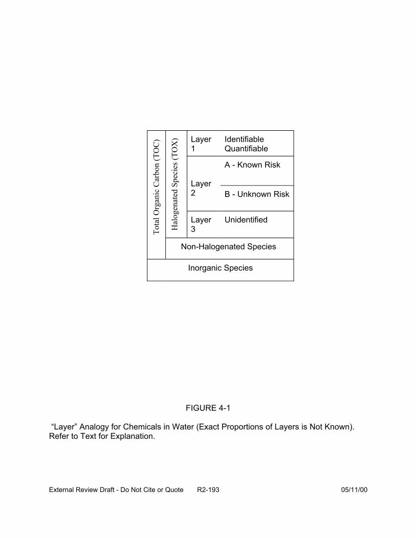
Tota
l Org
anic
Car
bon
(TO
C)
Hal
ogen
ated
Spe
cies
(TO
X) Layer
1 Identifiable Quantifiable
Layer 2
A - Known Risk
B - Unknown Risk
Layer 3
Unidentified
Non-Halogenated Species
Inorganic Species
FIGURE 4-1
“Layer” Analogy for Chemicals in Water (Exact Proportions of Layers is Not Known). Refer to Text for Explanation.
External Review Draft - Do Not Cite or Quote R2-193 05/11/00
The analyses conducted by Richardson (1998) to identify DBP by treatment type
have some limitations. There is some uncertainty that all of these compounds are DBP
and that they were not produced by the analytical procedure itself. For the ones that
have been identified, many have no occurrence data in the environment and no toxicity
measures; they may only represent a portion of what is really there. Of the unknown
material, some of it is hard to isolate and identify (more polar compounds). The
molecular weights of these compounds are unknown; compounds with high molecular
weight are generally thought to cause less toxicity.
All layers can be further divided (independently) into those chemicals believed to
be associated with a specific risk endpoint such as cancer, developmental or
reproductive risk (denoted “h” in the pre-workshop report, U.S. EPA, 1999) and those
not associated with that endpoint. There may be some misclassification of these; that’s
one (minor) uncertainty.
It is conceptually easier to forget about the finished water and concentrate
attention on this collection of DBP. For the halogenated DBP, for practical reasons,
consider all concentrations (in the water) as measured in TOX equivalents (regardless
of whether those concentrations are known or not). Then, in order to talk about the
concentrations of the DBP relative to each other, further normalize all concentrations by
the total concentrations. For example, if attention is momentarily focused on the
chlorinated DBP, this total concentration is measured by TOX.
The halogenated DBP are thereby partitioned by layer and endpoint association
into six mutually exclusive groups. For Layer 1, sufficient information is available to
conduct a quantitative risk assessment; concentrations and potencies are available.
External Review Draft - Do Not Cite or Quote R2-194 05/11/00
Naturally there is uncertainty, but this uncertainty is partially handled by the evaluation
in the CRFM case study (U.S. EPA, 1998). Additional uncertainties derive from
variation among water systems, variation in water source, temporal variation, and so on.
Assessing these uncertainties is relatively straightforward and may be in part
accomplished with the ICR data.
Relatively little is known about Layers 2 and 3. To estimate their contribution to
risk, it is tempting to suppose that the DBP in Layer 1 are a “representative” sample of
all the DBP. They must be representative in terms of:
• relative concentration distribution,
• univariate distribution of potencies, and
• apportioning of risk endpoints.
If Layer 1 chemicals were representative in these senses, then standard
statistical estimators could be applied to estimate the risk from the DBP in Layers 2 and
3. The uncertainty in the estimates would depend strongly on: variation in relevant
properties of DBP in Layer 1 (in the bullets above) and the proportion of all DBP within
Layer 1.
As discussed in Section 3.5, there is variation in TOX and the concentration of
certain Layer 1 DBP vary as a function of temperature. This suggests that Layers 2 and
3 constitute between less than 50% to more than 90% of all the DBP (again confining
discussion to the halogenated DBP).
Unfortunately, there are many reasons to suppose that the DBP in Layer 1 are
not representative of all DBP. Layer 1 DBP are (relatively) well known and well-studied.
This means that they have been suspects in observed exposures are readily identified
External Review Draft - Do Not Cite or Quote R2-195 05/11/00
and quantified, and so on. Most of these properties are closely related to chemical
structure, including being relatively light, uncomplex (few rings, bridges, heteroatoms,
etc.), and non-polar. By contrast, Layer 2 DBP are not as common or as well-studied,
so they may have systematic structural differences (on the whole) compared to Layer 1
chemicals, indicating potentially different modes of action in an organism and different
toxic endpoints. Even worse, chemicals in Layer 3 definitely have different chemical
structures (sufficiently so to make them difficult to identify, much less quantify, in an
aqueous solution).
Without any more information, one cannot say much more about Layer 3
chemicals than that they are chlorinated and may have potencies lying anywhere in the
range of potencies observed for any chlorinated compound—or even beyond, as the
MX example suggests. (MX was recently discovered, is chlorinated, and has the
highest mutagenicity potency yet observed.) Is there another MX lurking in Layers 2
or 3?
Further, many of these systematic differences among the layers may work to
make chemicals in Layers 2 or 3 systematically different in properties than those in
Layer1. Thus, any hope that differences might “cancel out” is not well-founded.
To reduce this enormous uncertainty, it is imperative to obtain some initial
information about what is in Layers 2 and 3. A statistically valid method would randomly
sample individual chemicals (stratification and proportional sampling are appropriate)
from these layers and attempt to measure important properties of the sampled
chemicals. At a minimum, relative concentration (in at least one water sample) and,
External Review Draft - Do Not Cite or Quote R2-196 05/11/00
very roughly, potency would be needed. Extrapolation from an LD50 assay would likely
suffice.
The method presented by EPA assumes that the known and unknown
compounds are equally toxic. This assumption could be examined by assembling
distributions of LD50s for each of the known and suspected compounds and comparing
these (Figure 4-2). LD50s can be found from experimental data or could be estimated
using Quantitative Structure Activity Relationship (QSAR) models. Mechanisms of
toxicity for the unknowns can only be assumed.
Different QSAR models (e.g., TOPKAT, OPP’s model, Case, Genetic Activity
Profile, or GAP data base) will yield various predictions that may conflict, so that
multiple “answers” are provided for analysis. However, this information could be
examined as a body of data for estimating the toxicity of the unknowns. Multiple
“answers” could be examined by expert judgment, perhaps by holding a workshop. One
important concept is to ask whether the QSAR models are asking the same questions
or whether they are designed to provide the same information that is directly
comparable. Another issue is to examine the misclassification errors for the various
models. A technique for looking at this body of QSAR data is to examine the range of
predictions (e.g., by ignoring the lower bound by using zero, but for the upper bound,
assuming a worst case, such as that all components are carcinogens, and making risk
predictions on that basis). For example, one might divide the LD50s of the known
components by a large number (Layton et al., 1987) that approximates their RfDs within
an order of magnitude (Equation 4-1). If total dose of the unknown compounds is less
than the sum of the known RfDs, then perhaps the unknowns could be ignored.
External Review Draft - Do Not Cite or Quote R2-197 05/11/00
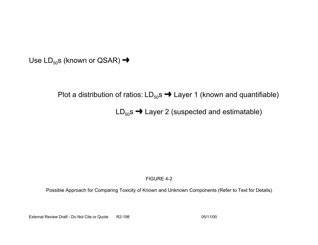
Use LD50s (known or QSAR) º
Plot a distribution of ratios: LD50s º Layer 1 (known and quantifiable)
LD50s º Layer 2 (suspected and estimatable)
FIGURE 4-2
Possible Approach for Comparing Toxicity of Known and Unknown Components (Refer to Text for Details)
External Review Draft - Do Not Cite or Quote R2-198 05/11/00

LD50 (4-1)
= RFDx10≈ 380,000
From a few such samples, one would begin to see what the distribution of
relative concentration of these chemicals is and what the distribution of potencies might
be. These distributions would be compared to those of Layer 1 to estimate, albeit
roughly, the degree to which properties of chemicals in Layers 2 and 3 compare to
those of Layer 1. In other words, there would be preliminary information—and
bounds—on the magnitude of differences among the layers: differences in
concentration, potency, even frequency of occurrence (if multiple finished water
samples were evaluated).
Such an analysis of the chemicals in Layer 3 cannot yet be conducted because
there is no sampling frame; the chemicals in this layer are not known and it is not known
whether it even exists. However, estimates of concentrations of chemicals in Layer 2
could be compared to TOX measurements; with enough replication (to overcome the
relatively large analytical variability in TOX measurements), the concentration of Layer 3
could be estimated. Further work at identifying individual chemicals in this layer would
be necessary if Layer 3 appeared to be “substantial.”
4.2.2. The MX Concern. The problem of characterizing Layers 2 and 3 is that there
may be one chemical present in relatively high concentrations that has a very large
potency. This possibility can be evaluated by estimating distributions of relative
concentrations of chemicals in Layers 2 and 3 and assigning potencies to them at
random from a distribution of potencies estimated for these layers. Such
External Review Draft - Do Not Cite or Quote R2-199 05/11/00

distributions—concentration and potency—must be based on some analysis of what is
in these layers and not just by using Layer 1 chemicals as a surrogate. Again, the
reason is that Layer 1 chemicals may behave very differently in these respects from the
other chemicals.
The uncertainty in the risk estimate therefore would depend on the variation in
concentrations and the variation in potencies. It seems reasonable to assume that
these two values would be independent. At one extreme, all concentrations (in a
particular layer) would be equal. To be concrete, suppose that Layer 2 constitutes 50%
of the DBP and that 50 chemicals are identified as its constituents. Then, at this
extreme (of maximum entropy), each chemical would constitute 1% of the DBP. The
distribution of potencies, F, when applied to this distribution of concentrations, would
produce a net distribution of risk (potency times concentration) equal to F/%50, which has
the same shape and location as F but a variance 1/50 that of F. At another extreme,
where one chemical accounts for essentially all the concentration in Layer 2, the risk
distribution would coincide with F. This simple calculation shows how the distribution of
risk depends on the estimated distribution of potencies of the Layer 2 (and Layer 3)
chemicals and why it is so important to estimate this distribution in a reasonable way.
4.2.3. Documenting Statistical Models for Risk Assessment. When assessing
uncertainty, it is important to write models that explicitly include random components.
The tendency to use omnibus, powerful estimation methods such as bootstrapping,
resampling, and Monte Carlo analysis is also a tendency to hide or overlook the
underlying statistical model. This can lead to the use of ad-hoc or inferior statistical
estimators.
External Review Draft - Do Not Cite or Quote R2-200 05/11/00
To avoid this tendency, and to document statistical procedures accurately, it will
be useful to record the models. For example, in Section 3.3, data relating dose to
fractional birthweight reduction for a group of chemicals was introduced. Each
birthweight reduction datum represented a group of measurements, each having a
reported variability (as a standard deviation, s). To combine this information, the idea of
a “TCA” equivalent for each chemical was introduced. This would be a chemical-
specific conversion factor 8(chemical) used to compare doses. The model is that at
equivalent doses, chemicals would produce equivalent fractional birthweight
reductions—plus a random error. This can be written as:
Birthweight reduction(chemical, dose) = (4-2)
Intercept + Slope x 8(chemical) x dose + e(chemical, dose)
where the e(chemical, dose) are (say) identically and independently distributed with
variance equal to s(chemical, dose). The s’s are given with the data and the values of
intercept, slope and l(chemical) are parameters to be estimated, subject to 8(TCA) = 1.
With a change of parameter from 8 to 8 x slope, this is readily seen to be a weighted
least squares (WLS) problem, whose solution is conventional. Thus, writing down the
model leads immediately to the appropriate statistical estimator of parameters and their
uncertainty. This often avoids having to re-invent appropriate estimators and it makes
the nature of the random component of the model apparent. It would be well to write all
statistical models used in the risk assessment in this (conventional) form.
In summary, improvements in the EPA’s method include putting distributions on
the variables in the equations for deriving the toxicity of the unidentified TOX, including
distributions on " h and the TOX amounts. It also might be interesting to statistically
External Review Draft - Do Not Cite or Quote R2-201 05/11/00
treat the question that if a progressive series of efforts to find DBP identifies fewer and
fewer DBP, then what is the likelihood of finding more? This could lead to some level of
confidence relative to whether the majority of the DBP have been identified. Finally, it
was suggested that the unidentified DBP could be treated only in a qualitative fashion.
4.3. CANCER RISK
Participants in this breakout group have a wide range of scientific and analytic
expertise. The members were: Robert Bruce, Josh Cohen, George Gray, Rick
Hertzberg, Mike Pereira, Charlie Poole, Rita Schoeny, and William Stiteler. This
breakout group addressed five key questions for assessing the potential cancer risks of
disinfection byproducts and characterizing the uncertainty in risk estimates:
• What approaches can incorporate the various types of data on health effects and still allow for comparing risks across treatment options?
• What questions regarding cancer could be addressed by expert judgment?
• How can the use of dose-response information for cancer risk be improved?
• How should we address the idea of a threshold for cancer?
• How should data be used for different tumor sites or effects in a mixture risk assessment?
The first two questions are discussed in Sections 4.3.1 and 4.3.2, respectively.
The next two questions are discussed together in Section 4.3.3, and Section 4.3.4
presents the discussion of the use of different sites or effects in mixture risk
assessment.
External Review Draft - Do Not Cite or Quote R2-202 05/11/00
4.3.1. What Approaches Can Incorporate the Various Data on Health Effects and
Still Allow for Comparing Risks Across Treatment Options? The group addressed
several important issues that were raised by this question including characterizing
uncertainty in hazard identification, reconciling epidemiologic and toxicologic data, and
identifying and quantifying often ignored sources of uncertainty in risk estimates based
on epidemiology.
The group believed that there was a need to characterize uncertainty in the
hazard identification step when evaluating carcinogens. Any hazard identification for a
general human population which relies on data from animal bioassays or occupational
exposure has an intrinsic degree of uncertainty. There are clearly differences between
chemicals in the degree of certainty that they are capable of causing cancer in humans.
To be most useful in a comparative framework, the uncertainty should be characterized
quantitatively so that it is reflected in the risk estimates that are compared.
The EPA’s cancer classification system under the 1986 guidelines is a sort of
qualitative uncertainty evaluation that may have some role in quantitative
characterization. It does not address questions of bioassay interpretation, including the
findings of widespread chemical treatment related decreases in tumor rates reported in
several recent publications (Linkov et al., 1998; Crump et al., 1999). There have been
papers making crude quantitative uncertainty adjustments to risk estimates based upon
cancer classification to facilitate comparisons. This approach does not help with
chemicals that have not been assessed by EPA, including the majority of DBP. The
group recommended further efforts to identify or develop methods for characterizing
uncertainty in hazard identification.
External Review Draft - Do Not Cite or Quote R2-203 05/11/00
Additional key hazard identification uncertainties in the DBP comparison involve
the comparison of chemical-specific toxicologic results with epidemiologic studies of
chlorinated drinking water. Foremost is the lack of concordance of tumor sites between
animal bioassays of DBP and the sites indicating possible increases in epidemiologic
studies. The group suggested that more efforts with both existing animal and human
data and further data development would be most helpful.
With current data, the use of PBPK models for different DBP, combined with
some notion of mode of action, might provide insight into patterns of tumor development
in animals and humans. Further work controlling for water source in epidemiologic
studies might help to identify key DBP associated with increased cancer risk. It was
also suggested that re-analysis of some ecologic studies might be useful. Finally, a
new meta-analysis with studies completed since 1992, including exploratory meta
analysis to identify important population characteristics, would provide valuable
information.
The group also suggested types of new studies that might shed some light on the
seeming disparities between epidemiologic and toxicologic results. Investigations in
animals and in vitro studies might identify the components of chlorinated water that are
associated with different types of cancer, studies of gene-environment interaction (e.g.,
CYP2E1, GST, acetyl) could identify particular subpopulations for further epidemiologic
study, and epidemiologic studies focusing on colon polyps might provide important
information.
A final source of uncertainty that the group agreed is important for
characterization comes from publication bias in epidemiologic studies. This could be a
External Review Draft - Do Not Cite or Quote R2-204 05/11/00
particular problem if studies of chlorinated drinking water that fail to find an association,
or find responses in different sites, are not published and not available for meta
analysis. Characterizing publication bias requires a great deal of effort to find studies
that are not generally available. It can be modeled and even corrected for, based on
new positive and non-positive studies, to quantitatively characterize the uncertainty.
The group also confronted the fact that quantitative estimates of risk based on
epidemiology are about 500 times higher than those based on animal toxicology data.
There was some discussion of the possible role of synergism, but the relatively low
levels of the DBP made this seem less likely. It is difficult to know if unidentified
components of treated water could account for the difference. One suggestion was a
quick calculation of the potency that would be required of an unidentified DBP to
account for the difference. The group postulated that the quantitative differences might
be due simply to the different scales used in epidemiology (where 0.1 increase in
relative risk can be quite large for a relatively common tumor) and toxicology-based risk
assessment that can calculate (extrapolate to) risk estimates in increments of 10-6 or
less.
4.3.2. What Questions Regarding Cancer Could be Addressed by Expert
Judgment? The group recognized that expert judgment (often implicit rather than
explicit) plays an important role in the risk assessment process, from identifying
chemicals, endpoints, and studies to addressing choices of models and other critical
assumptions. The field of decision analysis recognizes explicit expert judgment as a
legitimate means for characterizing uncertain model parameters with little or no directly
applicable data or that require the synthesis of several lines of evidence. It was, of
External Review Draft - Do Not Cite or Quote R2-205 05/11/00
course, recognized that the expert judgment process must be open and transparent with
recognition of the potential for bias or conflict of interest.
The cancer breakout group focused on the use of expert judgment to address
uncertainties in several key cancer risk assessment assumptions and as a guide to
uncertainty or sensitivity analysis of existing models.
The key assumptions that may benefit from expert judgment if a best estimate of
risk is to be constructed are:
• whether or not the agent is a human carcinogen,
• if there is non-linearity for carcinogenic action at a specific dose level or dose rate, and
• the mode of action of the compound.
Each of these issues requires synthesis of many different lines of empirical
evidence and biologic theory. Expert judgment, when subject to the disciplines
discussed in the expert judgment section (Section 3.10) may allow quantification of the
certainty of carcinogenicity or the threshold dose level (including uncertainty).
Judgment about the mode of action question is a prerequisite to addressing the
question of carcinogenicity or shape of the dose response curve.
In addition to estimating uncertain parameter values, the group recognized that
expert judgment could help in analyzing and evaluating current risk models. There was
a great deal of discussion around the need to disaggregate the epidemiology data and
extract results from the meta-analysis. It was also suggested that expert judgment
could help define appropriate ranges to use in sensitivity analysis of influential model
parameters. There was also a recommendation that expert judgment be used in
External Review Draft - Do Not Cite or Quote R2-206 05/11/00

understanding different methods of quantification from epidemiology, and for limiting the
studies to be analyzed, for plausibility.
Finally, the group discussed the potential for expert judgment to evaluate the
chemicals being investigated (e.g., the apparent discordant results from toxicology and
epidemiology for bladder cancer). It was recognized that this might be an example of
the sort of question that would more usefully be advanced by more analysis or
experimentation rather than expert judgment relying on relatively few data. Another
suggestion was to use QSAR to prioritize uncharacterized DBP for study and use expert
judgment for further processing or reducing the list of chemicals.
4.3.3. How Can the Use of Dose-Response Information for Cancer Risk be
Improved? How Should We Address the Idea of Low Dose Non-Linearity for
Cancer? These questions were discussed together. The group thought these
questions were tightly linked and were dependent on the understanding of the mode of
carcinogenic action of each specific compound. Since the comparative framework
requires best estimates of risk, it was recognized that this question did not focus on
“defaults” or conservative assumptions, but rather on how to judge the weight-of-
evidence for a specific mode of action for a specific chemical. The group recognized
that there is additional scientific uncertainty in linking particular dose-response models
to different modes of action.
The question of response thresholds is critical primarily when significant
extrapolation is needed from experimental or observational exposure to those of
interest. In the case of DBP, extrapolation is necessary when using animal bioassay
data from studies with exposure thousands, or even tens of thousands, of times higher
External Review Draft - Do Not Cite or Quote R2-207 05/11/00
than exposures in finished drinking water. The epidemiologic data are based on
exposure to finished water and have no need for extrapolation. However, the
uncertainty in the epidemiologic data are so great that it will be difficult to clearly
distinguish a threshold from a nonthreshold dose-response.
“Practical thresholds”, which some described as a level of response that is not
distinguishable from background responses, were discussed. It was not clear what
level of sensitivity or specificity of a test was necessary to establish a response as
similar to background. Some proponents believed these “practical thresholds” could
then be the launching point for applying EPA’s new cancer guidelines. There was
concern in the group with the way in which margin-of-exposure calculations (based on
the new EPA guidelines) could be used in risk comparisons since no explicit risk
estimates are made (see Figure 4-3). The group recognized that the question of
combinations of threshold carcinogens needs more work. Accumulation of hundreds of
near thresholds may be unacceptable.
The discussion of thresholds and low dose non-linearity raised several important
points of scientific uncertainty for the assessment of risk from threshold compounds.
First, the question of independence or commonality of modes of action is critical to
understanding if risks of threshold chemicals should be treated independently or
combined. The question of dose-addition versus response addition was discussed in
some detail along with attributes of modes of action or responses that would support
either notion. There was concern that high-dose toxicologic tests might demonstrate
interactions that might not occur, or might be different, at lower exposures.
External Review Draft - Do Not Cite or Quote R2-208 05/11/00
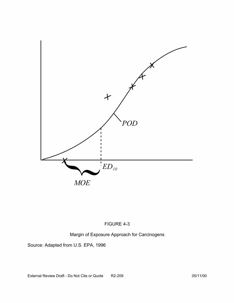
FIGURE 4-3
Margin of Exposure Approach for Carcinogens
Source: Adapted from U.S. EPA, 1996
External Review Draft - Do Not Cite or Quote R2-209 05/11/00
The question of what degree of similarity of mode of action would negate the
assumption of independence was recognized as very difficult. There are the questions
of high and low dose interactions mentioned above. It was recognized that a particular
toxic endpoint (e.g., liver tumors) might arise from many different mechanisms, which
may or may not be independent. Another possibility is commonality of a rate-limiting
step or a common pathway, but not necessarily the same main mode of action. This
raises the question of how identical modes of action need be and how, or whether,
classes of compounds can be identified for which the independence assumption is
invalid. It was suggested that the key would be to look for a common mode of action or
point of intersection in the biologic pathway. Some examples offered included changes
in methylation patterns, depletion of GSH or SAM, or changes in the hormonal systems.
The group suggested that if a common point in pathway, which affects the rate-limiting
step, cannot be found, then there is no need for response addition, but instead, risks
should be added.
Finally, there was some discussion of the different ways in which standard
models used in epidemiology address independence of events. Independence of
mechanisms is difficult to imagine because mechanisms for the same effect usually
have components in common. (Trivially, one must have a uterus to develop
endometrial cancer.) Where P(A) and P(B) are the probabilities of being susceptible to
the effects of A and B on the same outcome, P(A&B) is the probability of being
susceptible to both effects, and A and B do not interact synergistically, the probability of
developing the outcome if exposed to A and B is P(A) + P(B) - P(A&B). Additivity of
effects would correspond to P(A) + P(B) and, therefore, some degree of sub-additivity is
External Review Draft - Do Not Cite or Quote R2-210 05/11/00
expected in the absence of synergism. If the susceptibilities to the effects of A and B
are uncorrelated, P(A&B)=P(A)P(B), which for carcinogenic effects would usually be a
very small probability. However, a correlation of susceptibilities due to a sharing of
complementary component causes between etiologic mechanisms involving A and B
would lead to P(A&B)>P(A)P(B). With a strong correlation of susceptibilities, the
competitive antagonism represented by P(A&B), described as response type 2 in the
formulation of Greenland and Poole 1988, could be appreciable.
On the other hand, synergism has been established epidemiologically (e.g.,
asbestos, smoking, and lung cancer). To complicate matters, epidemiologists regularly
assume synergism by assuming uniformity (homogeneity) of relative risks (or odds
ratios). Uniformity of relative risk or odds ratios corresponds to additivity of the natural
logarithm of RR or OR, not additivity of risk or of risk difference, as in toxicological
interaction analysis of quantal response (see, e.g., Helwett and Plackett, 1979). When
epidemiologists assess “interaction”, they are almost always assessing departure from a
null state of (often substantial) synergism.
If one is looking for explanations for higher potency estimates from the
epidemiology of a mixture than from the toxicology of one compound at a time,
synergism is a more viable candidate than competitive antagonism separate (though not
necessarily independent) effects.
4.3.4. How Should Data be Used for Different Sites or Effects in a Mixture Risk
Assessment? This discussion was sharpened by a presentation on the current
thinking within EPA about risk assessment of mixtures. The group addressed several
issues related to the differences between response addition and dose addition. The
External Review Draft - Do Not Cite or Quote R2-211 05/11/00

discussion touched on several points discussed under previous questions including the
built-in assumption of synergism (as discussed above) in many epidemiologic models.
First, the group pointed out that response addition is not affected by site of action
as long as the individual dose-response model is probabilistic risk. Again, it was
recognized that if a chemical is considered “nonlinear” for cancer dose-response, then
no probabilistic risk is estimated and there is real difficulty with response addition under
this scheme. One suggestion that was offered, if the MOE approach is used, is to
consider a blend surface and connect the resulting doses reached by the MOE method
for each one.
The difficulty of even identifying potential interactions was highlighted again with
the observation that high dose interaction may be different from low dose interaction.
There was considerable discussion about whether the usual cancer interaction studies
(e.g., initiation-promotion, co-carcinogenesis) can even identify, or refute, situations in
which the assumption of independence is appropriate.
The group did recommend that the EPA investigators further evaluate
proportional response addition as a means to combine dose-response data when risks
are characterized using a MOE approach (Figure 4-4). In the area of dose addition,
several questions were raised, including the appropriateness of adding points of
departure (i.e., ED05s) and how to handle compounds with different weights of evidence
for both carcinogenic potential and mode of action. The breakout group was quite
adamantly against the combining of tumors from human studies. There were concerns
about differential uncertainty in the magnitude of the effect, different confounders with
different effects for different sites, and very different biological pathways leading to the
External Review Draft - Do Not Cite or Quote R2-212 05/11/00
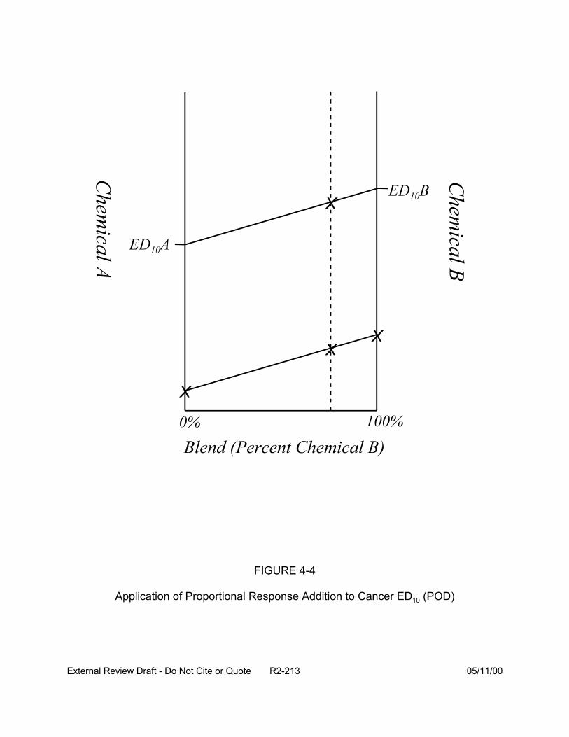
FIGURE 4-4
Application of Proportional Response Addition to Cancer ED10 (POD)
External Review Draft - Do Not Cite or Quote R2-213 05/11/00
tumors. There was also concern about potential double counting in the use of vital
statistics in risk estimation.
As an approach to many of the questions raised in the breakout session, the group
suggested that further exploration of the analysis be conducted as part of the proposed
change to the MCLG for chloroform. This might allow understanding of ways in which
uncertainties were, and were not, characterized well and might allow for some
generalization to other cases.
4.4. REPRODUCTIVE AND DEVELOPMENTAL TOXICITY GROUP
The participants in this break out group discussion were: Bruce Allen, Joan
Colman, Dale Hattis, John Lipscomb, and Jeff Swartout.
4.4.1 Improving the use of Animal Developmental and Reproductive Toxicity Data.
Choices must be made when analyzing animal developmental (and, in general, other
reproductive) toxicity tests. The breakout group attempted to identify a process, the first
step of which was the appropriate use of an animal data set – i.e., the topic discussed
here – but which also included issues related to the extrapolation of animal data to
humans (discussed in Section 4.4.2).
As with all analyses of toxicity data, a careful toxicological review and evaluation
should initiate the process. Specifically, with respect to the desired dose-response
analysis, one would be interested in the presence of dose-related effects (resorptions,
fetal deaths, malformations, and perhaps variations, are the most common quantal
effects that, along with fetal weight, would be typically considered). One might apply
statistical tests to look for evidence of a dose-related trend in incidence or level of effect
to identify the effects that suggest that the compound in question causes developmental
toxicity. Assuming that the study meets requirements considered toxicologically
External Review Draft - Do Not Cite or Quote R2-214 05/11/00

necessary for sufficient quality, these endpoints would be the set that would then be used
in the subsequent steps (dose-response analysis and extrapolation to humans).
A major issue of the use of laboratory animal developmental toxicity models for
prediction of human risk is the inconsistent concordance of specific effects between test
animals and humans. Laboratory developmental toxicity studies, however, are valuable
for predicting human developmental effects in the general sense. Another possible
limitation in the modeling of developmental toxicity studies is that individual fetus data are
not generally reported in the literature, requiring separate modeling of each endpoint. For
the DBP analysis, however, such data are available. Therefore, one approach to
assessing human risk from animal developmental toxicity data is to consider modeling
the risk of any treatment-related developmental effect, rather than focusing on a specific
effect. The general approach would be to aggregate the observed effects in the animal
bioassay prior to running the chosen dose-response model. A key issue in this
aggregation is the choice of endpoints to aggregate. Should all endpoints be lumped
together, or should they be combined on the basis of some classification? Examples of
classifications are type of malformation (e.g., visceral, skeletal or external), mechanistic
class, or continuous vs. quantal.
The breakout group, consistent with thinking among people who have conducted
dose-response modeling for developmental toxicity risk assessments, considered that it
appeared to be more appropriate to model individual embryo/fetal responses, as opposed
to litter-based summaries of response (e.g., litter with one or more affected fetus are
considered to be the responding litters); this was particularly true for quantal responses.
Therefore, for quantal responses, a model like the log-logistic model with underlying beta-
binomial response variability would be recommended for modeling a single quantal
External Review Draft - Do Not Cite or Quote R2-215 05/11/00
endpoint. Such models account for the correlated nature of the results from typical
developmental toxicity data sets (and from many reproductive toxicity data sets) an allow
one to get estimates of the fetal probabilities of response as a function of dose or
exposure (and other covariates such as litter size). Of course, other particular model
forms (such as those suggested by Rai and Van Ryzin many years ago or more recently
by NCTR) could be used in place of (or in addition to) the log-logistic form (these models
are discussed in Section 3.2). One could get some sense of model dependency (model
uncertainty) by applying more than one model to any particular data set.
For quantal endpoints, one can estimate the dose corresponding to a particular
level of response – often referred to as an EDx or a BMDx. (The choice of the value of
“x” depends on the objective of the scientist for extrapolating from the animal test results
to humans.) A traditional BMD analysis would pick a BMD05 (based on the results of
Allen et al., 1994), that would subsequently be used with some uncertainty factors to get
an RfD. The extrapolation approach proposed by Dale Hattis, referred to here as the
lognormal model of tolerances, would estimate the ED50, which in subsequent steps
would be used to estimate the median of the human lognormal tolerance distribution (see
Section 4.4.2).
For continuous endpoints, such as birth weight, it is not so clear how to model
dose-response relationships. One could turn such endpoints into quantal endpoints by
selecting a cutpoint to dichotomize normal and abnormal levels (e.g., normal vs.
abnormally low birth weights). One could then apply the log-logistic model (or some
similar model) to the now-quantal representation of the weight response. Alternatively,
one could model changes in the continuous variable itself (i.e., changes in mean birth
weight) as a function of dose. The results of such modeling could be used in at least two
External Review Draft - Do Not Cite or Quote R2-216 05/11/00

ways. First, they could be linked to sequella known or thought to be caused by changes
in the continuous endpoint (e.g., infant mortality linked to low birth weight, or infertility
linked to low sperm count) by additional modeling – with the notion that the sequella
would be the factors used to estimate a dose-dependent probability of a response of
concern. Alternatively, the continuous measure itself could be used to determine “risk,”
where in this instance, the risk at a dose would be determined by the likelihood that a
fetus would fall above or below some cutpoint. The idea of the cutpoint is exactly the
same here as discussed earlier in this paragraph – it separates normal from abnormal –
but note that it is only considered after the modeling is conducted. The endpoint could be
defined explicitly – based on toxicological considerations related to biological significance
– or it could be defined implicitly, based on the amount of variation observed in the test
animals (e.g., control animals) such that it represents a point relatively far out in the tail of
the distribution. Either way, the likelihood defining the risk is determined by looking at the
implied probability of being above (or below) the cutpoint defined by the dose-specific
mean predicted by the model and the variance around that mean (usually also estimated
from the data). Gaylor and Slikker (1990) and Crump (1995) have discussed this issue in
general; Kavlock et al. (1995) have looked at some of these issues in relation to
developmental toxicity.
Another alternative to modeling each selected endpoint separately is to model
several endpoints together using a multinomial model. Such models treat the possible
outcomes subsequent to implantation (resorption, fetal death, malformation, and
variations in birth weight) as a vector of responses that are modeled together to account
for possible intrafetal correlations among them. The multinomial modeling approach is a
bit more complicated and uses some different statistical approaches (generalized
External Review Draft - Do Not Cite or Quote R2-217 05/11/00
estimating equations for example), but there may be some instances where such an
approach might be appropriate. Ryan, Catalano, Gaylor, and Chen have all published on
this topic (see discussion in Section 3.2).
4.4.2. Predicting Human Risk from Animal Developmental and Reproductive Data.
The group discussed a variety of approaches for projecting human risks under two broad
headings of quantal vs. continuous animal effect data.
For quantal effect data, there are three main choices: the BMD, ED50, and slope
factor.
An adaptation of the EPA’s standard benchmark dose approach, incorporating
relevant uncertainty factors, is one approach that could be used for quantal data. In this
type of analysis, a point of departure is first selected from the animal dose response data.
Typically, analysts use the ED05, the dose (in mg/kg) expected to produce a 5% excess
incidence of the response in question over background, or the LED05—the lower 95%
confidence limit on that dose, as estimated from a standard dose response model. This
“benchmark dose” is then used to project a human RfD with the application of a list of
standard uncertainty factors—usually tenfold for projections from animals to humans,
tenfold for possible differences in sensitivity among humans, etc. The RfD thus
calculated is assumed to represent a human population threshold—a dose that is below
all the thresholds for response of individual people in a potentially exposed population. If
some people are potentially exposed at levels above the RfD, then individual risks are
projected by drawing a straight line between the assumed zero risk point at the RfD and
the expected incidence (e.g., 5%) at the benchmark dose. In more advanced
applications, pharmacokinetic or allometric (e.g., dose per unit body weight3/4) scaling
adjustments could be used to translate the benchmark dose into human equivalents.
External Review Draft - Do Not Cite or Quote R2-218 05/11/00
Additionally, distributions (for example, see Swartout et al., 1998) rather than point
estimates could be used for the uncertainty factors. An advantage of this approach is
that it is a relatively modest adaptation of the standard approach for noncancer risk
assessment. It incorporates a concept of population thresholds, which has been a
standard assumption by many toxicologists. It should be understood, however, that this
approach will not provide a convenient way to utilize new relevant information (e.g.,
human variability data for pharmacokinetic and pharmacodynamic parameters putatively
relevant to different toxicants and background rates of reproductive impairment and
developmental anomalies in humans.) It is expected that this approach will generally
lead to predictions of zero expected incremental risks because disinfectant byproduct
exposures are expected to be below the calculated RfD in nearly all cases.
A second way to analyze quantal data is to use the animal data only to identify the
kinds of effects produced by specific toxicants and associated potencies, indexed as an
ED50 (log normal model of tolerances). Human low dose risks are then projected using
generic information about human variability in the several steps from exposure through
response utilizing recently compiled human variability information (Hattis, 1997, 1998;
Ballew and Hattis, 1989; Rees and Hattis, 1994). Important issues for this approach are
the assumed form for the distribution of human threshold doses and the degree of spread
(e.g., geometric standard deviation [GSD]) of that distribution. Substantial changes in
calculated low dose risks can be expected to result from different distributional forms
(e.g., assuming a mixture of two or three lognormal distributions corresponding to
different genders or genetic variants of an important single-gene determinant of
susceptibility) or from different plausible values for the GSD. For these analyses, the
latter type of uncertainty is quantified by assuming that the toxicant under study is a
External Review Draft - Do Not Cite or Quote R2-219 05/11/00
random draw from a series of toxicants/effects whose susceptibility variabilities are
documented in the existing data base (either the whole data base or a putatively relevant
subset can be selected depending on the available information about the toxicant). An
advantage of this approach is that it recognizes the possibility that segments of the
human population may differ widely in susceptibility, and that in light of the fact that there
is some “background” rate of different developmental anomalies, reproductive
impairments, and other physiological failures, some people may well be very close to
critical values of relevant physiological parameters required to maintain normal
functioning. Existing analyses of the human variability data tends to support approximate
log-normality for distributions of pharmacokinetic and pharmacokinetic factors, without
obvious limits that might be expected under the generic assumption of population
thresholds. This approach also provides a ready means to accommodate new
information about relevant animal/human differences in average susceptibility/thresholds
and about human variability in pharmacokinetic or pharmacodynamic parameters. A
disadvantage is that this approach involves a noticeable departure from previous EPA
risk assessment practice and conclusions for non-cancer effects at levels of exposure
below the RfD (or their equivalents). This approach will lead to the projection of finite
risks for DBP (and estimates of uncertainty) at current exposure levels. Many, if not all,
of these projected risks are likely to be below limits of detection in epidemiologic studies.
The current EPA slope factor analysis is another option for handling quantal data.
However, this option was not discussed extensively by the breakout group. A
disadvantage of this approach is that it assumes a low dose linear dose-response
relationship that is generally at variance with the assumed homeostatic, threshold
mechanism assumed for most developmental and reproductive effects.
External Review Draft - Do Not Cite or Quote R2-220 05/11/00
For continuous parameters thought to be important for human effects, the
breakout group discussed two alternatives: changing the continuous response to a
quantal response or modeling dose-response relationship for the continuous endpoints.
The first approach is to quantize the response in animals (e.g., choose a “cutpoint”
such as a 5% reduction in fetal weight from the control average as indicating an “effect”),
and treat the effect by the quantal analysis techniques described above (discussed in
Section 4.4.1).
Alternatively, the dose-response relationship for the continuous endpoint in
animals could be modeled, projected to humans using a pharmacokinetic or allometric
dose scaling procedure, and then the implications for human risk using human data
interpreted in the context of the continuous parameter (or its human analog) to human
clinical outcomes of concern. Such an analysis should, of course, be limited to
parameters that do have human analogs that are strongly related to adverse outcomes of
concern. For example, the fetal weight reductions seen for various DBP could well be
predictive of fetal growth retardation and, therefore, reductions in birth weight for a
constant gestational age. Relationships between birth weights and outcomes of concern,
such infant mortality, can then be used to project human risks. In the reproductive area,
relationships between sperm counts and male fertility can also be used to estimate
effects either in terms of the fraction of couples presenting themselves for infertility
treatment (in a type of analysis pioneered by Meistrich and Brown (1983) or in terms of
the distribution of times to conception. The latter type of information is being prepared for
imminent publication by Eric Clegg of EPA ORD in Washington (Clegg, 1999). An
advantage of the use of continuous intermediate parameters such as birth weights is that
they are more amenable to epidemiologic study and measurement of population effects
External Review Draft - Do Not Cite or Quote R2-221 05/11/00
than rare quantal effects. The committee wishes to encourage epidemiologic study of
relationships between DBP exposures and these types of continuous intermediate
parameters that are likely to be predictive of rarer quantal endpoints of ultimate concern.
4.5. MIXTURES RISK CHARACTERIZATION
Participants in this breakout group discussion were: Joan Colman, Richard
Hertzberg, Jennifer McLain, Chandrika Moudgal, Glenn Rice, Rita Schoeny, William
Stiteler, and Clifford Weisel. This group addressed the questions posed in Section 4.0,
with the exception of Questions 2 and 8. The following sections summarize the
discussion of this breakout group.
4.5.1 Identification of Approaches that Incorporate Data on DBP Health Effects
into the Risk Assessment. The breakout group suggested several approaches: a
thorough review of the literature on complete mixtures (including in vitro studies);
application of three types of data analyses to evaluate additivity (multinomial, response-
addition, and proportional response addition); comparison of the results from
epidemiological and toxicological studies for consistency in health outcomes for individual
DBP or for mixtures of DBP. It was thought that a data base of individual studies exists
that has not been considered in its entirety. In trying to compare risks of DBP from
different treatment plants, it was suggested that modeling of risk using both a Monte
Carlo simulation (to estimate the range of risk estimates across the population served by
the plant) and a sensitivity analysis (to evaluate what factors in the different treatment
conditions accounts for variability in the risk) be conducted. These approaches are
described further in the sections that follow.
4.5.2 Improving the Current Approach to Estimate the Risks Posed by DBP
Exposures. A concern of the group was the discrepancy between effects found in
External Review Draft - Do Not Cite or Quote R2-222 05/11/00

epidemiological studies and toxicological laboratory studies. It was suggested that all
existing data be reviewed in order to better plan future whole mixture laboratory testing.
It is important to conduct such studies on reasonable representative samples,
recognizing that the composition of DBP differs with treatment type and location.
Methods need to be developed for comparing whole mixture with component studies,
and for combining such studies to get an improved real mixture risk estimate.
Current approaches of risk assessment do not consider additive effects. If there
are additive effects, their inclusion in the component approach to risk analysis would
result in improvement in the risk estimate. Modeling approaches can provide guidance
on the potential toxicity of compounds. Methods such as QSAR and Monte Carlo can
be applied to better understand the uncertainties in the risk assessment. However,
expertise in these areas is mandatory by the individuals applying them. One concern in
the current use of Monte Carlo analysis in risk assessment is that proliferation of
computer programs that allow for Monte Carlo analysis to be applied by untrained
individuals to any data set. This proliferation of the use of Monte Carlo simulation has
resulted in statistical analyses being conducted without proper consideration to the
underlying assumptions of that analysis. It was highly recommended that statisticians
who are appropriately trained in the evaluation of distributional data be included in both
designing and conducting studies that use Monte Carlo methods of analyses.
External Review Draft - Do Not Cite or Quote R2-223 05/11/00
4.5.3. Handling the Toxicity of DBP, or of Identified DBP, for which Little or No
Data Exist. Two methods for evaluating potential risk associated with DBP for which
little toxicity data exist is the use of QSAR and expert judgment to predict the probability
that a compound can cause a particular adverse health outcome. QSAR, which is
based on comparing descriptors within the molecular structure of the unknown chemical
to a training set of compounds of known toxicity, does not estimate potency and is
currently used for single compounds, not mixtures. Expert judgment relies on the
opinions of scientists in the field to predict the potential risk for untested compounds.
The group considered that both expert judgment and QSAR model selection, have
potential in prioritizing which DBP has the highest potential risk. It was suggested that
each procedure be run on the same set of chemicals for comparison. However, it was
noted that expert judgment is a time- and personnel-intensive process, so it can have a
limited application. Different QSAR models also exist and should be considered for use;
the same set of chemicals should be run through each model for comparison.
External Review Draft - Do Not Cite or Quote R2-224 05/11/00
4.5.4. Handling the Concept of Threshold and the Unidentified DBP. The doses
associated with human exposure to DBP are all below the levels administrated to
animals, making extrapolation necessary and the existence of a threshold effect level an
important consideration. The major concern among the mixture group was whether
unidentified chemicals may produce ‘surprise’ interactions even at low doses. Two
major considerations in determining the likelihood of toxicological interactions among
DBP mixtures are that the DBP are present at low concentrations in drinking water and
that a large number of compounds remain unidentified. Typically, little interaction is
expected at the doses associated with exposure to DBP in drinking water. It was the
consensus of the group that at the known current concentrations, synergistic
toxicological interactions will not occur. However, the large number of uncharacterized
compounds preclude completely ruling-out the possibility, although this was a low
probability event. An additional consideration that may result in possible interactions is
whether there could be accumulation of DBP in the body from the constant exposure or
whether there could be an accumulation of impacts of the hundreds of different
chemicals, each individually at a low level, but all acting (by the same mechanism) on
some precursor stage leading to an adverse health effect.
The use of whole mixture testing can help describe or bound the contribution of
the unidentified chemicals without doing individual compound tests. It was recognized,
however, that the composition and concentration of the “unidentified” DBP changes with
treatment alternative or geographic location, making selection of a representative
mixture for testing difficult. The group also was concerned about the need to evaluate
multiple health endpoints, and whether and how to focus on one or a few effects. The
External Review Draft - Do Not Cite or Quote R2-225 05/11/00
question was raised as to the need to use a more conservative model than response
addition so that the unidentified DBP are at least partly considered in the analyses.
Cancer, developmental, and reproductive effects have all been suggested to be
associated with exposure to DBP. The mechanism of action for each effect may be
different. Designing a study to test whether a mixture-effect exists first requires that the
health endpoint of concern be defined. It was strongly recommended that a
comprehensive review of previous studies on mixtures and components, both from a
perspective of animal studies and chemical characterization of the DBP, be conducted
before designing future studies. There was no consensus of whether concocted
mixtures or whole mixture extracts would provide a better approach for the animal
studies. The use of concocted mixtures would allow for alteration of the mixture by
spiking it with a known toxic agent to evaluate the plausibility of any observed effects
and environmentally realistic doses. The use of whole mixtures would allow for
evaluation of representative DBP mixtures without assumptions as to what the
biologically active components are. Selecting a real-world representative DBP mixture
is problematic because the components and concentrations of the unknown portion (as
well as the characterized portion) of the DBP are site-, season-, and treatment-type
specific. Differences in toxicological study outcomes and epidemiological outcomes can
occur depending on the DBP(s) used or present in each study. The mixtures present in
the positive epidemiologic studies (disinfection by chlorine or chloramine, levels of
bromide in the water, character of the precursor organic matter) should be used to
provide guidance as to what mixtures should be used in future toxicologic studies. The
External Review Draft - Do Not Cite or Quote R2-226 05/11/00

concocted and whole mixture studies can provide complementary data and the research
program should reflect the combination of the results from each type of study.
4.5.5. Interpretation of Human Developmental and Reproductive Risks Based on
Animal Data. A series of questions were raised in recognition of the magnitude of the
issues. Are there different kinds of sensitivity windows (of exposure) for the reproductive
and developmental risks, so that the likelihood of co-occurrence of two such effects is
small? How can continuous data be incorporated with quantal response data?
It was suggested that multiple effects might be modeled with a multinomial model
rather than with a series of individual binomial models. For example, one approach is to
score each fetus, with any developmental effect, as a responder. Risk curves could then
be generated for “developmental” as a category of effect for each of the chemicals
individually. The risk for the mixture might then be calculated by applying proportional
response addition across all of the compounds considered.
The group noted that lifetime risk for developmental and reproductive risks are not
adequate since there are different kinds of sensitivity windows (of exposure) for the
different effects. The likelihood of two such effects occurring together is small. While not
discussed extensively by the group, a potential issue is the appropriateness of summing
the risks if different DBP affect development at different stages or critical periods. If
considering risk/pregnancy, then it appears to be an appropriate approach, unless the
occurrence of an effect early in development precludes the occurrence of an effect later
in development. For example, the haloacetic acids and haloacetonitriles that have been
tested for developmental toxicity have a spectrum of effects in the postimplantation
period including postimplantation loss, depression of fetal body weight and crown-rump
length, and visceral and skeletal malformations. Thus, for these DBP, the critical periods
External Review Draft - Do Not Cite or Quote R2-227 05/11/00
appear to be similar. Should additional data indicate preimplantation effects, however,
the approach of summing the risks could be reconsidered.
It was recognized, but not discussed at length, that genotoxic effects may have an
impact on development. The possibility that subtle genotoxic changes from one or more
DBP may render an organism more susceptible to additional genotoxic effects from other
DBP should be investigated.
4.5.6. Summary. The breakout group agreed that additive methods of risk are plausible
for low doses even for unidentified compounds; QSAR and Monte Carlo approaches can
be applied to evaluating risk, which then can be added to gain better understanding of
many mixture issues if adequate expertise is available.
The breakout group recognized that they proposed no solution(s) on how to
combine different types of reproductive data; how sensitivity windows could affect
combining developmental and reproductive endpoints; or how to quantitatively bound
DBP and then eliminate some as not a concern.
4.6. UNCERTAINTY AND VARIABILITY GROUP
Participants in this breakout group discussion were: Bruce Allen, Brenda Boutin,
Josh Cohen, Dale Hattis, William Huber, Jeff Swartout, and Linda Teuschler.
This group tried to address five issues: approaches for evaluation of uncertainty
and variability; cancer slope factor uncertainty; noncancer dose-response analysis
uncertainty; uncertainty in exposure and concentration data; and uncertainties associated
with mixtures that contain unknown DBP with unknown toxicity characteristics. Each of
these major topics is discussed below.
4.6.1. Approaches for Evaluation of Uncertainty and Variability. It is important in
theory (and sometimes difficult in practice) to distinguish between variability and
External Review Draft - Do Not Cite or Quote R2-228 05/11/00
uncertainty. Variability denotes real differences that exist, as, for example, among
various members of a well-defined population with respect to some variable such as body
weight. The variable(s) of interest do not all have the same value across members of the
population, (i.e., there is heterogeneity so that they display a distribution of values within
the population in question, and are, therefore, determined to have a variability of some
magnitude). The magnitude of the variability depends on the degree of difference in the
parameter values within the population.
Uncertainty denotes a state of imperfect knowledge. In the context of risk
assessment, one is typically concerned with uncertainty about the values of variables that
are required to characterize risk. Uncertainty can, and does, relate to measures
characterizing the distribution of a variable within a population, such as the average value
and the variability around the average. Notably, estimates of the magnitude of the
variability of variable within a population are almost always subject to uncertainty.
Ignoring, for the moment, measurement errors (that add uncertainty simply
because the act of measuring is imperfect), uncertainty about the values of means and
variances (the two common characterizations of a variable’s distribution within a
population) arises because of the limited number of observations available to estimate
their magnitudes. In extreme, but all-to-frequent cases, no observations may be
available to estimate means and variances for the population of interest; in such cases,
inferences based on observations in other populations or other circumstantial evidence
may be required to make any guesses about the means and variances of concern.
Clearly, there may be a great deal of uncertainty about the estimates in those instances.
Indeed, that inferential (cross-population) uncertainty is the biggest source of
uncertainty affecting the risk assessment of DBP mixtures. Stochastic uncertainty (the
External Review Draft - Do Not Cite or Quote R2-229 05/11/00

uncertainty associated with direct estimation of a mean and variance, or any other
distributional parameter, using observations from the population of interest), does
contribute to overall uncertainty in DBP mixture risk assessments, but it is suspected that,
in relative terms, the magnitude of that uncertainty is small. Moreover, methods for
characterization of stochastic uncertainty are well developed. For example, confidence
limits for means (or for variances) are well-known and universally recognized methods for
expressing stochastic uncertainty. In contrast, methods for characterization of inferential
uncertainty have not been developed, and expression of such uncertainty tends to be
less quantitatively rigorous.
In the following sections, these considerations will be explored specifically in the
context of the DBP mixtures risk assessment. Because a Monte Carlo approach that
distinguishes between variability and uncertainty has been (rightly) proposed as a means
of summarizing the results of the DBP mixtures risk assessment (U.S. EPA, 1999),
specific references to implementation of a Monte Carlo procedure are included.
4.6.2. Characterization of Uncertainty Influencing Estimates of the Cancer Slope
Factor. Slope factors were one set of key parameters used to characterize the risks
associated with exposures to DBP mixtures (U.S. EPA, 1999). Along with other
parameters, the slope factors are treated as uncertain values that are input into U.S.
EPA’s Monte Carlo procedure in order to determine uncertainty and variability
associated with the risk estimates. Because of their use in the Monte Carlo procedure,
it is important to get a good characterization of the uncertainty of the slope factors.
However, the characterization of uncertainty for the cancer slope factor for each
DBP in the EPA pre-meeting report (U.S. EPA, 1999) reflects only stochastic
External Review Draft - Do Not Cite or Quote R2-230 05/11/00
uncertainty. Moreover, that characterization is not done appropriately. U.S. EPA (1999)
documents an approach based on an assumption that for the slope factor “the
distribution of plausible values is lognormal, with a geometric mean equal to the
estimated MLE, and a 95th percentile equal to the upper 95% confidence limit on the
slope.” (U.S. EPA, 1999, p. 40). This is just one of many instances where confidence
limits and percentiles of distributions are erroneously represented to be the same thing.
Moreover, the additional assumption about the underlying distribution of a slope factor
estimate (lognormality) is unnecessary and problematic.
More appropriately, quantification of the stochastic component of the uncertainty
for a chemical’s slope factor can be computed using resampling (bootstrap) techniques.
Such techniques repeatedly compute the cancer slope factor for different, synthetic data
sets. The synthetic data sets are constructed by assuming that the response rates
within each dose group in a bioassay follow binomial distributions. The underlying
probability of response for each dose group, from which the synthetic numbers of
responders are generated, can be determined by either the observed fraction of
affected animals in that group in the original experiment, or the modeled value of the
probability of response. The modeled value is derived from the assumed dose-
response curve at that dose-group’s dose; the model-based approach uses the MLE
parameter values from the fitted dose-response function. Several members of the
group recommended the latter approach.
It must be recognized that even in the above discussion, there are elements of
inferential uncertainty that impinge on the stochastic uncertainty estimates for the slope
factor. The slope factor is itself based on an extrapolation to low doses of a DBP, doses
External Review Draft - Do Not Cite or Quote R2-231 05/11/00
for which there are no direct observations. The slope factor estimate depends on the
suspected probability of response in animals exposed to those low doses, and
therefore, one is at least implicitly making inferences about the hypothetical population
of animals exposed to those low doses, based on the observations of populations of
animals exposed to higher doses. A dose-response relationship is assumed to govern
the relationship between high-dose and low-dose responses, but one must remember
that the assumed relationship is merely that, an assumption.
In addition to the stochastic uncertainty related to a slope factor estimate, one
that is amenable to an improved characterization, there are many other inferential
uncertainties. Not least of these is the issue of extrapolating the animal-based estimate
to the required estimate relevant to humans. Some assumptions are required to make
that extrapolation, assumptions that are themselves uncertain and which lead to
uncertainty with respect to the resulting quantitative values of a human-relevant slope
factor.
Data comparing potency in animals and humans for a generic set of chemicals
could be used to quantify the distribution of plausible human potency estimates
associated with the DBP-potency estimates inferred from the animal toxicity data sets.
The Allen and Crump analysis of this issue may serve as a useful starting point (Allen et
al., 1988a, 1988b; Shipp et al., 1989). Analyses reported by Dale Hattis based on the
data compiled by Allen et al. suggest that the distribution of human potency estimates
corresponding to a slope-factor estimate inferred from an animal toxicity data set can be
characterized as lognormal with a GSD of approximately 10 (see Section 3.1).
Therefore, in a Monte Carlo exercise, when determining the value of a human slope
External Review Draft - Do Not Cite or Quote R2-232 05/11/00
factor to use for a set of simulations, one might take the animal-based slope factor
estimate (which itself could be sampled from the distribution representing its stochastic
uncertainty) and then sample from a lognormal distribution having a mean equal to that
animal-based estimate and a GSD of 10.
With respect to the contribution of stochastic uncertainty to total uncertainty, the
following general considerations are relevant. The total slope factor uncertainty for a
specific chemical should depend on the magnitude of that chemical’s stochastic
uncertainty component; the procedure outlined in the preceding paragraph does that by
making the starting point (the animal-based slope factor estimate) subject to the degree
of uncertainty dictated by the stochastic component. It is therefore the case that the
estimated (uncertain) value of the human slope factor is a function of the measured
animal slope factor and its attendant uncertainty. However, it may be unlikely that this
adjustment of the estimate of total uncertainty to reflect the magnitude of the stochastic
component of uncertainty for a specific chemical will have a substantial impact. The
variance of the inferential uncertainty (log10) is approximately 1 (recall that the
suggested GSD for that uncertainty is 10); the variance of the stochastic uncertainty
(log10) was suggested to be in the neighborhood of 0.1 (the GSD for stochastic
uncertainty may be around 2, typically, if one wants to characterize stochastic variability
in terms of a lognormal distribution). Overall variance, as the sum of these two
contributors, would therefore reflect primarily that contributed by inferential uncertainty.
In the discussions above, other important sources of, or contributors to,
uncertainty have been ignored. Measurement error was already mentioned as a
possible source of error; it is likely that its contribution will be more significant with
External Review Draft - Do Not Cite or Quote R2-233 05/11/00
respect to exposure and concentration estimation (see Section 4.6.4 below) than in
relation to slope factor estimation. However, some of the more important concerns
related to slope factors include the existence of multiple (animal) data sets and possible
disagreements among them with respect to slope factor estimates. As a specific
concern, the treatment of negative studies requires some serious consideration.
Moreover, risk estimates from different sites for cancer may be problematic.
Mechanistically, the cell that causes a cancer in the kidney must be a different cell from
the one that causes cancer in the liver. It is not clear if an additive approach (e.g., using
a proportional response addition approach) would be appropriate or how one would
handle the correlations between risk estimates obtained from different cancer sites.
If one adds to these (and other) concerns technical questions regarding the
dependency of a resampling technique on maximum likelihood estimation (with possible
resolutions related to use of a variety of models, likelihood contours, and
variance/covariance matrices for parameter estimates), it is clear that not all of the
issues related to uncertainty associated with slope factor estimation have been
resolved. It is equally clear that careful deliberation needs to be applied to approach a
satisfactory resolution of the representation of uncertainty concerning DBP slope
factors.
External Review Draft - Do Not Cite or Quote R2-234 05/11/00

4.6.3. Characterization of Uncertainty Influencing Estimates of the Noncancer
Dose-Response. As in the case of the cancer slope factors, it was suggested that the
U.S. EPA (1999) method for dealing with noncancer risks could be improved in some
very specific ways. As a simple example, the use of the linearized multistage model
imposes assumptions that are consistent neither with biologically plausible models of
these health effects nor with other noncancer risk analyses that have appeared in the
literature. For developmental toxicity endpoints, in particular, the models chosen are
less than optimal.
Also paralleling the discussion above concerning cancer slope factors, it is
recognized that the only uncertainty dealt with in the U.S. EPA (1999) assessment of
noncancer risks is stochastic uncertainty. The uncertainties related to non-stochastic
contributors are very likely to have the greatest impact on uncertainty about human
noncancer risks associated with DBP mixtures.
Lately, the use of benchmark dose (BMD) estimates has become standard for
noncancer risk analyses. Using an estimate of a dose associated with some fairly low
level of response (e.g., an effective dose [ED] associated with less than 10% risk for a
quantal endpoint), and a lower confidence limit on that dose to account for stochastic
uncertainty, such a risk assessment would apply “uncertainty factors” to determine a
dose that was considered to be suitably safe. The uncertainty factors can be viewed as
“accounting for” non-stochastic uncertainties such as animal-to-human extrapolation.
Benchmark dose estimation, being reliant on uncertainty factors to derive a “safe
dose,” may not be the most appropriate method in the context of the DBP mixtures risk
exercise, for the following reasons. The DBP assessment requires risk estimates
External Review Draft - Do Not Cite or Quote R2-235 05/11/00
associated with all potential exposure levels. Strictly speaking, the benchmark dose
approach would not supply those estimates; the BMD methodology specifically avoids
using the dose-response model predictions at low levels of exposure because, by and
large, the models fit to the data are not selected with biological relevance in mind.
Therefore, for doses well beyond the range of the observations, the model predictions
may not be good. The use of uncertainty factors in the BMD approach is included as a
way around this difficulty; if chosen appropriately, the application of uncertainty factors
to BMD estimates yields safe exposure levels (albeit ones with no explicit statement of
associated risk).
As an alternative, a modified form of dose-response assessment followed by
extrapolation to humans was suggested. Suppose that a dose-response model is still fit
to available animal bioassay data, but instead of estimating an ED10 or less, one
estimates an ED50. The proposal is that the ED50 estimated in that manner be assumed
equal to a human ED50 (when scaled appropriately to account for body weight and/or
other relevant species differences). Then, probability of response at other dose levels
could be determined by assuming some distribution and a variance for response
probability around that ED50.
Dale Hattis has proposed that the distribution of probabilities of response be
considered to be lognormal, and that this distribution’s variance can be inferred from
observed distributions of human physiological responses measured in the context of
exposure to various substances. Hattis has estimated the implied GSD for the
distribution of human response thresholds. He has also quantified the uncertainty in
External Review Draft - Do Not Cite or Quote R2-236 05/11/00
this estimate (refer to Sections 3.1, 3.2, and 4.4). Some analogous approaches would
have to be developed for use with continuous response data.
Clearly, both the estimates of risk associated with a given human dose and the
uncertainty in that estimate would need to be available to inform the two-stage Monte
Carlo procedure proposed by U.S. EPA (1999). A careful and deliberate examination of
the data used to estimate human variability (and the uncertainties associated with it)
must be undertaken, because the use of the “surrogate” variability data (i.e., data that
considers variations in human pharmacokinetic and pharmacodynamic parameters that
may have more or less relevance to the chemical responses of interest) is the epitome
of inferential uncertainty itself. Moreover, the other issues discussed in connection with
cancer slope factors (multiple studies, negative results, different endpoints) are
pertinent considerations here. Clearly, a much more elaborate development of a
noncancer risk assessment method appropriate for DBP mixtures is required and will
entail considerable extra effort.
4.6.4. Uncertainty Associated with Exposure and Concentration Data. It would
appear to be the case that both exposure and concentration estimates are subject to
variability and uncertainty. Even at the most fundamental level, concentrations of some
of the DBP are uncertain for any given treatment system simply because the identity of
those DBP is unknown. Above and beyond this fundamental difficulty (which is
discussed somewhat more in the next section), there are uncertainty and variability
issues that need to be recognized in relation to both concentration and subsequent
exposures. Measurement errors associated with collection of concentration data (for
External Review Draft - Do Not Cite or Quote R2-237 05/11/00
which there is substantial laboratory involvement) and tap water intake data (based on
survey results) are likely to be a significant contributor to uncertainty.
Again, some technical difficulties in characterizing the variability in known DBP
concentrations can be found in U.S. EPA (1999). For example, the assumption of a
normal distribution and fixing the value of non-detects at half the detection limit both
hamper effective estimation of an appropriate frequency distribution. For concentration
data, a lognormal distribution (or a mixture of distributions including a lognormal
component) would be a more suitable assumption. Maximum likelihood estimation
techniques do not require specification of a value for non-detects; those techniques
should be applied without such unnecessary data manipulation.
In addition, because tap water intake is one of the key parameters determining
exposure (once a set of DBP concentrations is given), some care must be taken in
interpreting and using the tap water intake data to derive distributions characterizing
variability and/or uncertainty. Of particular concern here is the lack of differentiation
between percentiles of consumption across individuals and percentiles across days of
consumption. It is believed that the available consumption data (presented in Ershow et
al., 1991) were averaged over 3-day periods. Thus, daily variation probably can not be
derived. But derivation of some sort of distribution for temporal variation might be
possible, and this would provide information different from that representing
interindividual variations. Such information might be important when considering the
impact of some noncancer endpoints, where (unlike the typical assumption for a cancer
risk assessment) a long-term average daily dose may not be the most appropriate
determinant of response.
External Review Draft - Do Not Cite or Quote R2-238 05/11/00

Even though these concentration and exposure parameters may be considered
to be better characterized as variable rather than uncertain, it is worth remembering that
populations are defined temporally as well as spatially. The data collected for tap water
intake, in particular, may be especially sensitive to temporal changes in the population.
In any case, with any of these parameters, one is extrapolating from one population to
another (possibly very similar) population, if for no other reason than the fact that DBP
concentrations and tap water intake are not things that “exist” and persist over extended
periods of time.
4.6.5. Uncertainty Associated with Unknown DBP Fractions. One of the biggest
sources of uncertainty for the entire DBP mixtures risk assessment is the treatment of
portions of that mixture that are unknown to one degree or another (further discussion is
presented in Section 4.2). It was suggested that the DBP might be characterized as
belonging to one of three “layers” and associated with any given endpoint as follows:
Layer 1 = identified DBP (known concentrations, toxicity data, and structures); • let a1 be the proportion associated with an endpoint
Layer 2 = unidentified DBP (names of some of those and their structures, with QSAR information, will be known, but toxicity data will be absent)
• let a2 be the proportion of this layer associated with an endpoint
Layer 3 = unidentified DBP (nothing is known about these except that they exist) • let a3 be the proportion of this layer associated with an endpoint
The a1 values are used in the U.S. EPA (1999) calculations of risk. Of course,
the a1 values are estimated and are subject to (considerable) error. Other uncertainties
associated with the DBP in layers 2 and 3 relate to the estimates of their concentrations
(Ci) and “potencies” (Si).
External Review Draft - Do Not Cite or Quote R2-239 05/11/00

While no specific suggestions were provided by the uncertainty/variability group
with respect to dealing with these uncertainties, some suggested approaches related to
the following. It might be important to look at trends in toxicity across layers (although
this will require additional toxicity testing and may be limited to the first two layers).
Molecular weights and polarity data might also be attainable and might be useful
surrogates for more detailed information, especially if the known toxicity data could be
related (even grossly) to such measures. Moreover, the information presented by Pat
Fair relating total TOX to specific by-products may help to quantify magnitudes (and
provide bounding estimates at the very least) (see Section 3.5).
Clearly, not many concrete suggestions for dealing with the uncertainties
associated with unidentified DBP were provided by this work group. This may be one
prime example of the degree to which “nonquantifiable” uncertainties dominate a risk
assessment. Even some nonquantitative representation of the most likely implications
of these uncertainties may be difficult. Nevertheless, summary tables enumerating all of
the sources of uncertainty (or forms of ignorance) associated with the DBP mixtures risk
assessment should be provided. Those tables might provide at least rough estimates of
the magnitudes of the associated uncertainties; estimates of the level of effort (in time
and money) required to reduce those uncertainties would also provide valuable
information to decision-makers and other users of the risk assessment. If presented
well, such a summary will go a long way toward making a DBP mixtures risk
assessment acceptable.
External Review Draft - Do Not Cite or Quote R2-240 05/11/00
4.7. TOXICOLOGY/EPIDEMIOLOGY AND EXPERT JUDGMENT
The participants in this breakout group were: Gunther Craun, George Gray, John
Lipscomb, Patricia Murphy, and Charlie Poole.
The group recognized that both epidemiologic and toxicologic approaches
contribute valuable information to the risk assessment process, but that there have
been difficulties incorporating the epidemiologic results into the quantitative risk
assessment. There is a need to better characterize the uncertainties associated with
the underlying epidemiologic literature and when attempting to quantify the human
health risks, it should be recognized that insufficient epidemiologic data are available to
establish a causal association between DBP and cancer or reproductive risks. There is
confusion among epidemiologists and toxicologists about how to interpret the findings or
the studies because of inherent differences in the design, execution, and analysis of the
studies. Of particular concern are the non-comparability of the water exposures
studied, methodological differences among the studies, internally inconsistent findings
within studies, and the lack of consensus regarding causality for bladder, colon, and
rectal cancers. The literature on reproductive and developmental effects is currently
too sparse to use for quantitative risk assessment. One of the problems in attempting to
interpret the epidemiologic findings is the incompletely presented dose-response
information by the study authors. Use of continuous data (where available) improves
both the sensitivity and the power of the analysis, and the panel recommended that
these analyses be conducted. As new studies are planned for this area, scientists
should consider the experience from the cancer epidemiology literature and strive to
avoid similar problems.
External Review Draft - Do Not Cite or Quote R2-241 05/11/00
The breakout group agreed that the issues that needed to be addressed by both
epidemiologists and toxicologists include:
• examining the sensitivities (range of) in humans and animals;
• explicitly considering humanly relevant exposures (levels, routes, cumulative, peak, etc.) and endpoints in the design of new toxicologic studies on DBP;
• quantitatively identifying the uncertainties in exposure-response analysis of the epidemiologic literature (only apply alternative models to the data, use the continuous data that exists);
• providing an explanation of the uncertainties involved;
• refraining from the use of a single value for risk; and
• increasing the understanding of problems associated with using a single aggregate number from a meta-analysis for regulatory decisions, specifically, and for
• assessing causality,
• guiding future research, and
• assessing sensitive subsystems and water treatment differences.
The breakout group recommended that an “expert” panel be convened to identify
the important issues regarding better characterization of the uncertainties associated
with interpreting the epidemiologic literature and how best to quantify the human health
risks of cancer and exposure to drinking water disinfectants and byproducts. Previous
reviews have identified many of these uncertainties and potential solutions may not
require a large investment of money and time. The discussion of these uncertainties at
the present workshop indicates the continued importance of attempting to resolve these
issues.
External Review Draft - Do Not Cite or Quote R2-242 05/11/00
Although the panel would not be engaged in the formal elicitation of expert
opinions, the selection of the individual panel members should be considered as
carefully as if that were the goal. The general composition of the panel should include
epidemiologists, toxicologists, and quantitative analysts who have had experience in
complex problem solving. The primary interest of the panel is to objectively evaluate
the current studies and analyses of their results, identify the uncertainties, and
recommend ways to reduce these uncertainties. They would also oversee the
implementation of projects and tasks specifically designed to address the relevant
issues and interact frequently with all investigators. The panel should consist of
persons who have not been involved in the design and/or conduct of the existing
studies, although these individuals would inform the panel in regard to the important
subject matter information. It is expected that the work of the panel would be long term
(1-2 years). The panel should be actively involved in helping to evaluate how
uncertainty can be reduced, designing or guiding the design of specific analyses to be
conducted, periodically be informed of progress on recommended analyses, and
providing feedback to the analysts. The group envisioned that panel meetings would be
held on a quarterly basis to effectively facilitate the implementation of their
recommendations (Table 4-2).
4.7.1. Issues for Blue Ribbon Panel Discussion. The following ten issues were
suggested by this breakout group for consideration by “Blue Ribbon Panel”.
• Must a meta-analysis produce a single summary effect estimate for each cancer?
A common view of meta-analysis is that its purpose is to produce a single
summary effect estimate. Further, a meta-analysis that does not produce such a
External Review Draft - Do Not Cite or Quote R2-243 05/11/00

TABLE 4-2
Objectives for a “Blue Ribbon Panel”
• frame the questions that need to be addressed,
• recommend appropriate analyses,
• set the range of input values for sensitivity analyses,
• conduct (with feedback loops) periodic assessment of status of work, new findings that become available, and inform and assist decision makers in the interpretation of new findings,
• provide feedback between analysts and those framing the issues, and
• consist of a multi disciplinary scientific group with
• “new blood”
• subject matter and general experts
External Review Draft - Do Not Cite or Quote R2-244 05/11/00
summary is often considered a “failed” meta-analysis. An alternative view is that much
can be learned from applying meta-analytic techniques to understanding differences
among the results from the various studies in relation to the ways the studies were
conducted, the populations studied, the exposures and exposure contrasts that were
examined, and the way the results were analyzed and presented. The two approaches
or motivations in meta-analysis, aggregation and explanation, should be viewed in the
context of three major purposes of meta-analysis: to assist in causal inference, to help
assess public health impact, and to guide future research. Thus, the alternative view of
meta-analysis’ purpose should be more widely publicized and adopted. The single
summary effect estimate seems to be of relatively little value for assessing the DBP-
cancer risk issue. The panel should consider these questions: Can a meta-analysis that
does not produce a single summary effect estimate assist in causal inference? If a
meta-analysis provides evidence that all the studies are not merely producing more or
less precise estimates of an effect measure that has a single, “one size fits all” value, is
a single summary adequate? How can a single summary estimate of effect guide future
research?
• “Inclusive” versus “best evidence” approaches to meta-analysis and quantitative risk assessment using epidemiologic data.
The epidemiologic literature on chlorinated drinking water and cancer may be
divided into three parts: (a) studies that are currently analyzed at the ecologic level; (b)
studies at the individual level that lack interview information; and (c) studies at the
individual level with interviews. An inclusive approach would involve reanalyzing as
many of the current ecologic studies as possible to make them individual-level analyses.
The approach would then include these studies and all individual-level studies, with or
External Review Draft - Do Not Cite or Quote R2-245 05/11/00

without interviews. The recent paper by Bukowski and Murphy (1998) took a “best
evidence” approach by confining the analysis to studies that were at the individual level,
that had interviews, that included incident cancer cases (as opposed to cancer deaths),
and that for which the exposure metrics were variations on the theme of cumulative
exposure (e.g., years of residence in communities with chlorinated water). Thus,
Bukowski and Murphy (1998) restricted their analysis to a subset of studies at the
individual level with interviews. An even more extreme version of the “best evidence”
approach would be to base quantitative risk assessments on each study with a
quantitative exposure metric, one by one. The choice between the inclusive and best
evidence approaches can have important implications. For instance, the best evidence
approach leads to reliance on a smaller data base with more stochastic uncertainty.
The inclusive approach, on the other hand, might require a reanalysis project to turn as
many of the currently ecologic studies into studies at the individual level. However, the
data base would be larger with less uncertainty.
• What can be done about publication bias?
Appreciable evidence of publication bias was present in the results extracted
from individual studies in the 1992 meta-analysis by Morris et al. (Poole, 1997; Murphy
et al., 1999; Poole and Greenland, 1999). If this evidence persists when the literature
search is replicated and brought up to date should a summary effect estimate be
produced anyway or is evidence of publication bias a contraindication to aggregation?
Can anything be done to lessen the impact of publication bias? The first of two general
options is to “beat the bushes” to find as many unpublished results as possible. This
approach is extremely time-consuming, expensive, and labor-intensive, as it requires
External Review Draft - Do Not Cite or Quote R2-246 05/11/00

personally contacting as many researchers as possible who might have unpublished
results on the topic. A second option is an analytic approach of conducting a sensitivity
analysis to model the unpublished results. This is a form of missing data imputation.
Statistical theoreticians in the field of meta-analysis are developing imputation methods
to model missing results due to publication bias. It may be worthwhile to see if any of
these methods are suitable for use in the literature on chlorinated drinking water and
cancer.
• How can exchangeable results be extracted from the individual studies?
Extracting results for meta-analysis from individual studies is a process fraught
with decisions, assumptions, and uncertainties. The goal should be to extract
“exchangeable” results: results that, by their nature, one would have no reason to
expect that they would differ quantitatively from each other. In the data of Morris et al.
(1992), this assumption is not met. A key impediment to exchangeability is the use of
different exposure metrics. Many, very dissimilar exposure metrics have been used in
studies of cancer and chlorinated drinking water. Some are based only on the
surface/ground or chlorinated/unchlorinated status of the community of residence of
cases and controls at the time of their deaths. Others include quantitative or semi-
quantitative information on concentrations of one or more chlorination by-products.
Some include residential histories over some or all of the lives of study subjects and
thus can support measures of cumulative exposure. These cumulative exposure
measures can differ fundamentally, however. Some may be years of residence in
“chlorination communities.” Others may be in the form of lifetime consumption of one or
more chlorination compounds (e.g., in milligrams) or in the form of lifetime cumulative
External Review Draft - Do Not Cite or Quote R2-247 05/11/00
exposure (e.g., microgram per cubic liter-years). Finally, a small number of studies take
interview information on amounts of tap water consumption into account. When studies
with polytomous exposure scales report results for categories (e.g., four categories of
“chlorinated water years”), options for extracting results include the contrast between
the highest and lowest categories, combining all categories but the lowest into a single
category, fitting a regression equation to the categorical effect estimates, or fitting a
linear (or legit-linear) regression or a more flexible regression to the individual,
continuously measured data. The choices, assumptions, and uncertainties involved in
putting the extracted results on a common, exchangeable footing are considerable in
this literature. The “Blue Ribbon” panel could consider the choices and assumptions
and make recommendations.
• What are the implications of evidence of overall heterogeneity?
Every worthwhile meta-analysis includes an overall assessment of heterogeneity
of the study-specific results. This assessment usually takes the form of a formal test of
the hypothesis of homogeneity. When the P-value from such a test is low, what should
the analyst do? Some would merely compute an overall summary effect estimate by
conducting a variance-inflating random-effects analysis. Others would consider the
evidence of heterogeneity as a contraindication to aggregation and would focus the
remainder of the analysis on a search for study characteristics that would explain
sizable portions of the heterogeneity. An ill-advised approach is to identify a single,
influential study that is responsible for more of the apparent heterogeneity than any
other study and to exclude that study. To debate and resolve the implications of
External Review Draft - Do Not Cite or Quote R2-248 05/11/00
evidence of heterogeneity for aggregative meta-analysis would be an important
contribution by the “Blue Ribbon” panel.
• Confounding by water source.
One of the earliest concerns in the epidemiologic literature on chlorinated
drinking water and cancer, raised as early as the study by Alavanja et al. (1978), is that
the distinction between chlorinated water and unchlorinated water is tantamount in most
studies to the distinction between surface water and ground water. Differences other
than chlorination between surface water and ground water thus create the potential for a
form of confounding that is built directly into the exposure scale in many studies and
that therefore cannot be controlled analytically. Of the existing studies, only those by
Brenniman et al. (1980) and Zierler et al. (1986) held water source constant.
Brenniman et al. confined their contrast of chlorinated and unchlorinated communities in
Illinois to those using ground water. Zierler et al. contrasted primarily surface-water
communities in Massachusetts using chlorination with those using chloramination. Few
if any municipalities that currently chlorinate would have the option of switching from
chlorinated surface water to unchlorinated ground water, or of switching from
chlorinated ground water to unchlorinated ground water. Thus, only the study by Zierler
et al. comes close to examining the actual choice faced by most community water
systems that currently supply chlorinated surface water to their customers: switching
from chlorinated surface water to the same surface water disinfected by some other
means. The implications of this lack of correspondence of the exposure contrast in
almost all studies in the currently available literature to the actual choices faced by
municipal water systems is a major source of uncertainty in this literature.
External Review Draft - Do Not Cite or Quote R2-249 05/11/00
• Confounding by other factors.
Confounding by factors other than water source is an additional source of
uncertainty in the studies of chlorinated drinking water and cancer. Some studies
completely lack information on cigarette smoking, for instance. Smoking has an
established association with bladder cancer and a possible or probable association with
colorectal cancer. What is the magnitude of these associations? How strongly, and in
what direction, might smoking be associated with measures of exposure to chlorination
byproducts in the study populations in this literature? Questions such as these need to
be answered to conduct sensitivity analyses of uncontrolled confounding, not only by
smoking, but by other factors as well. Possible risk factors for colorectal cancer include
dietary fiber, physical activity, and others. Incompletely controlled confounding is
another problem. In some studies, the information on smoking comes largely from
surrogate respondents such as next-of-kin. Inaccuracies in this information may
adversely affect the degree to which the confounding can be controlled. In some
studies, age has been controlled very approximately, for instance, by dividing it into 10-
year or even 20-year intervals. For some cancers, the relation to age is so strong (often
expressed as a power function), that risk may vary as much as two-fold across just a 5-
year age range. Since the exposure metrics in some of the studies are measures of
exposure duration that extend to 30, 40, 50, or 60 years and more, the control for
confounding by age should be as complete as possible.
• Control selection in case-control studies.
Nearly all of the studies in this literature are case-control studies. The validity of
the control groups, therefore, is a major concern. Ideally, the control group accurately
External Review Draft - Do Not Cite or Quote R2-250 05/11/00
represents the joint distribution of the exposure and of all unmatched confounders in the
study population. Thus, a random sample from a roster of the study population would
be preferred. Unfortunately, such a roster is virtually never available. In some studies,
the controls are persons who died of causes of death other than cancer. Most of these
controls would be expected to be persons who died of cardiovascular disease. Is the
occurrence of death from cardiovascular disease the equivalent of random selection
with respect to water chlorination, smoking, and other potential confounders? In other
studies, random-digit telephone dialing was used to select controls. This procedure is
known to produce control groups of lower socioeconomic status (SES) than the
populations they are intended to represent. Might this bias with respect to SES produce
a bias with respect to water chlorination? These and other questions concerning the
validity of control selection need to be addressed on a study-by-study basis.
• Other study characteristics.
It may be possible that characteristics of studies other than those mentioned
above are important determinants of the results these studies produce. Two commonly
examined characteristics are the cohort versus the case-control design and year of
publication. Year of publication is often an important indicator of publication bias and
validity. The earliest studies often tend to be those that report the strongest
associations. Often, as a research program matures, better methods are brought to
bear. One characteristic of special importance in this literature might be geographic
variation in the constituents of the source water. The bromine content, to take but one
example, might bear importantly on the mixture of chlorination byproducts to be
produced in the finished water.
External Review Draft - Do Not Cite or Quote R2-251 05/11/00
• Interaction.
Many of the studies examine interaction, either formally by including product-
interaction terms in logistic regression models, or informally by visual inspection of
stratified results. Gender and smoking are popular choices as variables with which to
examine interactions with measures of exposure to chlorinated drinking water.
Unfortunately, these analyses, whether formal or informal, are virtually always
conducted on the multiplicative scale. This fact makes the assessment of interaction in
the epidemiologic studies differ fundamentally from the assessment of interaction in the
toxicologic literature, where the analysis is almost always conducted on the additive
scale. In epidemiologic terminology, there is no interaction on the multiplicative scale
when the relative risk or odds ratio for one factor (e.g., chlorinated water) is
homogeneous or uniform across levels of the other factor (e.g., smoking), and there is
no interaction on the additive scale when the risk difference is homogeneous or uniform.
Evidence of etiologic synergism (or antagonism) is provided by evidence of statistical
interaction on the additive scale, not on the multiplicative scale. Thus, when
epidemiologic investigators ask whether, for instance, the relative risk estimates for
chlorinated water differ between smokers and non-smokers, they are looking for
departures from a null state (equal relative risks in the two groups) in which a
substantial degree of synergism is built in. Viewed in another way, when there is no
etiologic synergism or antagonism, one should expect the relative risk for the exposure
to be lower among smokers than among non-smokers. The analysis of interaction on
the multiplicative scale in epidemiologic studies may have created a considerable
degree of confusion in the interpretation of their results. (Assessment of interaction on
External Review Draft - Do Not Cite or Quote R2-252 05/11/00
the additive scale can be conducted in case-control studies, as long as neither of the
factors has been used to match the controls to the cases.)
4.8. CONCLUSIONS, FUTURE RESEARCH AND RECOMMENDATIONS OF THE BREAKOUT GROUPS
4.8.1. Exposure. The exposure breakout group participants offered several
recommendations for assessment of DBP mixtures. Multi-route exposures should be
considered by the EPA as they are likely important for risk assessments for DBP. The
inhalation exposure for volatile DBP and dermal exposure to highly lipophilic DBP can
result in exposures equivalent to ingestion for median water uses. Thus, when
comparing risks from different water sources and treatments practices (which may result
in different types of DBP and concentrations), it is critical to include all exposure routes.
Full exposure models linked to a physiologically-based pharmacokinetic (PBPK) model,
if available, should be conducted to estimate human doses. Exposure models should
be evaluated with experimental and field data.
Potential population distributions of exposure should be considered rather than
point values; this is especially important for susceptible or high-risk subpopulations.
Some people may have much higher inhalation exposures to volatile DBP and may also
have higher dermal exposures (e.g., frequent swimmers, users of hot tubs and spas).
Identification of these subgroups and estimation of their ranges of exposures needs to
be considered. Consumption data are needed; several data sets are just becoming
available, but they may not provide the information needed for pregnant and lactating
women. Data are needed on skin permeability, especially for young children.
Recreational exposures to DBP through chlorinated swimming pools need to be
quantified.
External Review Draft - Do Not Cite or Quote R2-253 05/11/00
In epidemiologic studies, full exposure models should incorporate the range of
water concentrations at both the treatment plant and within the distribution system over
the etiologically relevant time period, changes in the mixture of DBP during the
exposure period if there have been changes in water sources or treatment practices,
water use and consumption patterns that may affect ingestion, inhalation, and dermal
exposures, other human behavioral activities or characteristics that may affect
exposure, and household/work place characteristics.
Long-term research goals should be to continue to invest time and efforts into
identifying chemicals in TOX and further identifying DBP that make up the unknown
fraction. It is important that specific DBP be identified and quantified, as the multi-route
exposure approach can be problematic for DBP that are not specifically identified and
when concentrations are not measured (e.g., compounds identified only as TOX). The
extrapolation of the unidentified DBP, based on a surrogate of TOX, is questionable.
Expert judgment could possibly be used to help characterize risks posed by TOX and
other non-identified DBP in populations. However, to obtain population distribution of
exposures, appropriately designed surveys may be better at providing missing data.
Volatile DBP may be good surrogates for inhalation exposure to unidentified DBP.
Identification of DBP from ozone, chloramine, and chlorine dioxide treatment
processes should also be long-term research goals. More data for chloramines, ozone,
and chlorine dioxide by-products are needed as well as predictive models of their
concentration at the water treatment plant and/or distribution system. There will be
sufficient data on concentrations of THM, HAA, bromate, and aldehydes in water
systems throughout the U.S. after the ICR data become available. These data can
External Review Draft - Do Not Cite or Quote R2-254 05/11/00
serve as inputs to existing mathematical models that predict distribution system
exposures, including concentrations at the tap.
Actual exposure data should be used to help define ratios of mixtures for
toxicology studies (i.e., brominated/non-brominated species). Ratios of mixtures should
also be considered when evaluating exposures in epidemiological studies.
More attention should be paid to the potential value of whole mixture testing.
Consideration should be given as to whether whole mixture testing will assist in
estimating risks.
4.8.2. Unidentified DBP. This breakout group thought that it is imperative to obtain
some information about the identified, but unquantified TOX, and also about the
unidentified TOX, in order to reduce the enormous uncertainty in the current risk
assessment. The participants suggested a statistically valid method that would
randomly sample individual chemicals (stratification and proportional sampling are
appropriate) from these groups and attempt to measure important properties of the
sampled chemicals. At a minimum, relative concentration (in at least one water sample)
and, very roughly, potency would be needed. Extrapolation from an LD50 assay would
likely suffice as a rough measure of potency.
The method presented by EPA (U.S. EPA, 1998, 1999) assumes that the known
and unknown compounds are equally toxic. The group suggested this assumption
could be examined by assembling distributions of LD50s for each of the known and
unknown compounds and comparing these. LD50s can be found from experimental data
or could be estimated using Quantitative Structure Activity Relationship (QSAR) models.
Mechanisms of toxicity for the unknowns can only be assumed.
External Review Draft - Do Not Cite or Quote R2-255 05/11/00
Different QSAR models will yield various predictions that may conflict, so that
multiple “answers” are provided for analysis. However, this information could be
examined as a body of data for the unknowns. Multiple “answers” could be examined
by expert judgment, perhaps by holding a workshop. A technique for looking at this
body of QSAR data is to examine the range of predictions. The result would be
preliminary information—and bounds—on the magnitude of differences among the
identified DBP-- differences in concentration, potency, even frequency of occurrence (if
multiple finished water samples were evaluated). Such an analysis cannot yet be
conducted on the unidentified DBP because there is no sampling frame, but the
concentration of unidentified chemicals could be estimated. Further work at identifying
individual DBP would be necessary if the concentration of this group appeared to be
“substantial.”
Improvements in the EPA’s method include putting distributions on the variables
in the equations for deriving the toxicity of the unidentified TOX, including distributions
on " h and the TOX amounts. It also might be interesting to statistically treat the
question that if a progressive series of efforts to find DBP identifies fewer and fewer
DBP, then what is likelihood of finding more? This could lead to some level of
confidence relative to whether the majority of the DBP have been identified. Finally, it
was suggested that the unidentified DBP could be treated only in a qualitative fashion.
4.8.3. Cancer. The group believed that there was a need to characterize uncertainty in
the hazard identification step when evaluating carcinogens. Any hazard identification
for a general human population that relies on data from animal bioassays or
occupational exposure has an intrinsic degree of uncertainty. To be most useful in a
External Review Draft - Do Not Cite or Quote R2-256 05/11/00
comparative framework, the uncertainty should be characterized quantitatively so that it
is reflected in the risk estimates that are compared. The group suggested that more
efforts with both existing animal and human data and further data development would
be most helpful.
With current data, the use of PBPK models for different DBP, combined with
some notion of mode of action, might provide insight into patterns of tumor development
in animals and humans. Further work controlling for water source in epidemiologic
studies might help to identify key DBP associated with increased cancer risk. It was
also suggested that re-analysis of some ecologic studies might be useful. Finally, a
new meta-analysis with studies completed since 1992, including exploratory meta
analysis to identify important population characteristics, could provide valuable
information.
The group also suggested types of new studies that might shed some light on the
seeming disparities between epidemiologic and toxicologic results. Investigations in
animals and in vitro studies might identify the components of chlorinated water that are
associated with different types of cancer, studies of gene-environment interaction (e.g.,
CYP2E1, GST, acetyl) could identify particular subpopulations for further epidemiologic
study.
A final source of uncertainty that the group agreed is important for
characterization comes from publication bias in epidemiologic studies. Attempts to
characterize, model, and even correct for publication bias, based on new positive and
non-positive studies, to quantitatively characterize the uncertainty, could be considered.
External Review Draft - Do Not Cite or Quote R2-257 05/11/00

Several key assumptions about carcinogenic DBP that may benefit from expert
judgment if a best estimate of risk is to be constructed are:
• whether or not the agent is a human carcinogen,
• if there is non-linearity for carcinogenic action at a specific dose level or dose rate, and
• the mode of action of the compound.
In addition to estimating uncertain parameter values, the group recognized that
expert judgment could help in analyzing and evaluating current risk models. In addition,
expert judgment had the potential to evaluate the chemicals being investigated (e.g., the
apparent discordant results from toxicology and epidemiology for bladder cancer). It
was recognized that this might be an example of the sort of question that would more
usefully be advanced by more analysis or experimentation rather than expert judgment
relying on relatively few data. Another suggestion was to use QSAR to prioritize
uncharacterized DBP for study and use expert judgment for further processing or
reducing the list of chemicals.
There was concern in the group with the way in which margin-of-exposure
calculations (based on the new EPA guidelines) could be used in risk comparisons
since no explicit risk estimates are made. The group recognized that the question of
combinations of carcinogens showing non-linearity at low dose needs more work. It
was recognized that if a chemical is considered “nonlinear” for cancer dose-response,
then no probabilistic risk is estimated and there is real difficulty with response addition
under this scheme. One suggestion that was offered, if the MOE approach is used, is to
consider a blend surface and connect the resulting doses reached by the MOE method
for each one. The group recommends that EPA further evaluate proportional response
External Review Draft - Do Not Cite or Quote R2-258 05/11/00
addition as a means to combine dose-response data when risks are characterized using
a MOE approach. In the area of dose addition, several questions were raised, including
the appropriateness of adding points of departure (i.e., ED05s) and how to handle
compounds with different weights of evidence for both carcinogenic potential and mode
of action.
As an approach to many of the questions raised in the breakout session, the
group suggested that further exploration of the analysis be conducted as part of the
proposed change to the MCLG for chloroform. This might allow understanding of ways
in which uncertainties were, and were not, characterized well and might allow for some
generalization to other cases.
4.8.4. Reproductive and Developmental. The breakout group thought that laboratory
developmental toxicity studies are valuable for predicting human developmental effects
in the general sense, despite inconsistent concordance of specific effects between test
animals and humans. For the DBP analysis individual fetus data are generally reported
in the literature, overcoming a possible limitation often seen in the literature. The
experts thought that EPA could consider modeling the risk of any DBP-related
developmental effect, rather than focusing on a specific effect. The general approach
would be to aggregate (e.g., type of malformation, mechanistic class, or continuous vs.
quantal the observed effects) in the animal bioassay prior to running the chosen dose-
response model.
The breakout group considered that it appeared to be more appropriate to model
individual embryo/fetal responses, as opposed to litter-based summaries of response;
this was particularly true for quantal responses. A model like the log-logistic model with
External Review Draft - Do Not Cite or Quote R2-259 05/11/00
underlying beta-binomial response variability would be recommended for modeling a
single quantal endpoint. Such models account for the correlated nature of the results
from typical developmental toxicity data sets (and from many reproductive toxicity data
sets) and allow one to get estimates of the fetal probabilities of response as a function
of dose or exposure (and other covariates such as litter size). Other particular model
forms could also be applied.
Another alternative to modeling each selected endpoint separately is to model
several endpoints together using a multinomial model. Such models treat the possible
outcomes subsequent to implantation (resorption, fetal death, malformation, and
variations in birth weight) as a vector of responses that are modeled together to account
for possible intrafetal correlations among them. While a bit more complicated, there
may be some instances where a multinomial approach might be appropriate.
For quantal effect data, there are three main choices for predicting human risk
from animal developmental and reproductive data: the BMD, ED50, and slope factor.
The dose corresponding to a particular level of response, often referred to as an EDx or
a BMDx, could be estimated. In more advanced applications, pharmacokinetic or
allometric (e.g., dose per unit body weight3/4) scaling adjustments could be used to
translate the benchmark dose into human equivalents. Additionally, distributions rather
than point estimates could be used for the uncertainty factors. It is expected that this
approach will generally lead to predictions of zero expected incremental risks because
DBP exposures are expected to be below the calculated RfD in nearly all cases.
A second way to analyze quantal data is to use the animal data only to identify
the kinds of effects produced by specific toxicants and associated potencies, indexed as
External Review Draft - Do Not Cite or Quote R2-260 05/11/00
an ED50 (log normal model of tolerances). Human low dose risks are then projected
using generic information about human variability in the several steps from exposure
through response utilizing recently compiled human variability information. An
advantage of the use of continuous intermediate parameters such as birth weights is
that they are more amenable to epidemiologic study and measurement of population
effects than rare quantal effects. A disadvantage is that this approach involves a
noticeable departure from previous EPA risk assessment practice and conclusions for
noncancer effects at levels of exposure below the RfD (or their equivalents). This
approach will lead to the projection of finite risks for DBP (and estimates of uncertainty)
at current exposure levels. Many, if not all, of these projected risks are likely to be
below limits of detection in epidemiologic studies.
The current EPA slope factor analysis is another option for handling quantal data,
but was not discussed extensively by the breakout group. A disadvantage of this
approach is that it assumes a low dose linear dose-response relationship that is
generally at variance with the assumed homeostatic, threshold mechanism assumed for
most developmental and reproductive effects.
For continuous endpoints, such as birth weight, it is not so clear how to model
dose-response relationships. One could turn such endpoints into quantal endpoints by
selecting a cutpoint to dichotomize normal and abnormal levels (e.g., normal vs.
abnormally low birth weights). One could then apply the log-logistic model (or some
similar model) to the now-quantal representation of the weight response. Alternatively,
one could model changes in the continuous variable itself as a function of dose. The
dose-response relationship for the continuous endpoint in animals could be modeled,
External Review Draft - Do Not Cite or Quote R2-261 05/11/00
projected to humans using a pharmacokinetic or allometric dose scaling procedure, and
then the implications for human risk using human data could be interpreted in the
context of the continuous parameter (or its human analog) to human clinical outcomes
of concern. Such an analysis should, of course, be limited to parameters that do have
human analogs that are strongly related to adverse outcomes of concern. For example,
the fetal weight reductions seen for various DBP could well be predictive of fetal growth
retardation and, therefore, reductions in birth weight for a constant gestational age.
Relationships between birth weights and outcomes of concern, such as infant mortality,
can then be used to project human risks. The committee encouraged epidemiologic
study of relationships between DBP exposures and these types of continuous
intermediate parameters that are likely to be predictive of rarer quantal endpoints of
ultimate concern.
4.8.5. Mixtures Risk Characterization. The breakout group suggested several
approaches to the EPA: a thorough review of the literature on complete mixtures
(including in vitro studies); application of three types of data analyses to evaluate
additivity (multinomial, response-addition, and proportional response addition); and
comparison of the results from epidemiological and toxicological studies for consistency
in health outcomes for individual DBP or for mixtures of DBP.
It was strongly recommended that a comprehensive review of previous studies
on mixtures and components, both from a perspective of animal studies and chemical
characterization of the DBP, be conducted before designing future studies. It was
thought that a data base of individual studies exists that has not been considered in its
entirety.
External Review Draft - Do Not Cite or Quote R2-262 05/11/00

The use of whole mixture testing can help describe or bound the contribution of
the unidentified chemicals without doing individual compound tests. It was recognized,
however, that the composition and concentration of the “unidentified” DBP changes with
treatment alternative or geographic location, making selection of a representative
mixture for testing difficult because the components and concentrations of the unknown
portion (as well as the characterized portion) of the DBP are site-, season-, and
treatment-type specific. Differences in toxicological study outcomes and
epidemiological outcomes can occur depending on the DBP used or present in each
study. The mixtures present in the positive epidemiologic studies (disinfection by
chlorine or chloramine, levels of bromide in the water, character of the precursor organic
matter) should be used to provide guidance as to what mixtures should be used in
future toxicologic studies. The concocted and whole mixture studies can provide
complementary data, and the research program should reflect the combination of the
results from each type of study.
It was suggested that multiple effects might be modeled with a multinomial model
rather than with a series of individual binomial models. The risk for the mixture might
then be calculated by applying proportional response addition across all of the
compounds considered.
The breakout group agreed that additive methods of risk are plausible for low
doses even for unidentified compounds; QSAR and Monte Carlo approaches can be
applied to evaluating risk which then can be added to gain better understanding of many
mixture issues if adequate expertise is available. In trying to compare risks of DBP from
different treatment plants, it was suggested that modeling of risk using both a Monte
External Review Draft - Do Not Cite or Quote R2-263 05/11/00
Carlo simulation and a sensitivity analysis be conducted. It was highly recommended
that statisticians who are appropriately trained in the evaluation of distributional data be
included in both designing and conducting studies that use Monte Carlo methods of
analyses.
The group considered that both expert judgment and QSAR model selection
have potential in prioritizing which DBP has the highest potential risk. However, it was
noted that expert judgment is a time- and personnel-intensive process, so it can have a
limited application. Different QSAR models also exist and should be considered for use;
the same set of chemicals should be run through each model for comparison.
4.8.6. Variability and Uncertainty. This group tried to address approaches for
evaluation of uncertainty and variability; cancer slope factor uncertainty; noncancer
dose-response analysis uncertainty; uncertainty in exposure and concentration data;
and uncertainties associated with mixtures that contain unknown DBP with unknown
toxicity characteristics.
A Monte Carlo approach that distinguishes between variability and uncertainty
has been (rightly) proposed as a means of summarizing the results of the DBP mixtures
risk assessment (U.S. EPA, 1999). However, the characterization of uncertainty for the
cancer slope factor for each DBP in the EPA pre-meeting report (U.S. EPA, 1999)
reflects only stochastic uncertainty. That characterization is not done appropriately.
There are many instances where confidence limits and percentiles of distributions are
erroneously represented to be the same thing. Moreover, the additional assumption
about the underlying distribution of a slope factor estimate (lognormality) is unnecessary
and problematic.
External Review Draft - Do Not Cite or Quote R2-264 05/11/00
Quantification of the stochastic component of the uncertainty for a chemical’s
slope factor can more appropriately be computed using resampling (bootstrap)
techniques. A model-based approach using the MLE parameter values from the fitted
dose-response function was recommended by several members of the group.
Other important sources of, or contributors to, uncertainty need to be considered.
The contribution of measurement error is likely ro be more significant with respect to
exposure and concentration estimation than in relation to slope factor estimation.
However, some of the more important concerns related to slope factors include the
existence of multiple (animal) data sets and possible disagreements among them with
respect to slope factor estimates. As a specific concern, the treatment of negative
studies requires some serious consideration. Risk estimates from different sites for
cancer may be problematic. If one adds to these (and other) concerns technical
questions regarding the dependency of a resampling technique on maximum likelihood
estimation (with possible resolutions related to use of a variety of models, likelihood
contours, and variance/covariance matrices for parameter estimates), it is clear that not
all of the issues related to uncertainty associated with slope factor estimation have been
resolved. Careful deliberation needs to be applied to approach a satisfactory resolution
of the representation of uncertainty concerning DBP slope factors.
As in the case of the cancer slope factors, it was suggested that the U.S. EPA
(1999) method for dealing with noncancer risks could be improved in some very specific
ways. As a simple example, the use of the linearized multistage model imposes
assumptions that are consistent neither with biologically plausible models of these
health effects nor with other noncancer risk analyses that have appeared in the
External Review Draft - Do Not Cite or Quote R2-265 05/11/00
literature. For developmental toxicity endpoints, in particular, the models chosen are
less than optimal. The only uncertainty dealt with in the U.S. EPA (1999) assessment of
noncancer risks is stochastic uncertainty. The uncertainties related to non-stochastic
contributors are very likely to have the greatest impact on uncertainty about human
noncancer risks associated with DBP mixtures. Lately, the use of benchmark dose
(BMD) estimates has become standard for noncancer risk analyses. Benchmark dose
estimation, being reliant on uncertainty factors to derive a “safe dose,” may not be the
most appropriate method in the context of the DBP mixtures risk exercise. As an
alternative, a modified form of dose-response assessment followed by extrapolation to
humans was suggested. Suppose that a dose-response model is still fit to available
animal bioassay data, but instead of estimating an ED10 or less, one estimates an ED50.
The proposal is that the ED50 estimated in that manner be assumed equal to a human
ED50 (when scaled appropriately to account for body weight and/or other relevant
species differences). Then, probability of response at other dose levels could be
determined by assuming some distribution and a variance for response probability
around that ED50.
Both the estimates of risk associated with a given human dose and the
uncertainty in that estimate would need to be available to inform the two-stage Monte
Carlo procedure proposed by U.S. EPA (1999). A careful and deliberate examination of
the data used to estimate human variability (and the uncertainties associated with it)
must be undertaken, because the use of the “surrogate” variability data (i.e., data that
considers variations in human pharmacokinetic and pharmacodynamic parameters that
may have more or less relevance to the chemical responses of interest) is the epitome
External Review Draft - Do Not Cite or Quote R2-266 05/11/00
of inferential uncertainty itself. Moreover, the other issues discussed in connection with
cancer slope factors (multiple studies, negative results, different endpoints) are
pertinent considerations here. Clearly, a much more elaborate development of a
noncancer risk assessment method appropriate for DBP mixtures is required and will
entail considerable extra effort.
Even though DBP concentration and exposure parameters may be considered to
be better characterized as variable rather than uncertain, it is worth remembering that
populations are defined temporally as well as spatially. Some care must be taken in
interpreting and using the tap water intake data to derive distributions characterizing
variability and/or uncertainty.
One of the biggest sources of uncertainty for the entire DBP mixtures risk
assessment is the treatment of portions of that mixture that are unknown to one degree
or another. In addition to the health endpoint of concern, other uncertainties associated
with the unidentified relate to the estimates of their concentrations and “potencies”. It
might be important to look at trends in toxicity across layers; molecular weights and
polarity data might also be attainable and might be useful surrogates for more detailed
information, especially if the known toxicity data could be related (even grossly) to such
measures. Information relating total TOX to specific by-products may help to quantify
magnitudes (and provide bounding estimates at the very least).
The group recommended summary tables enumerating all of the sources of
uncertainty (or forms of ignorance) associated with the DBP mixtures risk assessment
should be provided. Those tables might provide at least rough estimates of the
magnitudes of the associated uncertainties; estimates of the level of effort (in time and
External Review Draft - Do Not Cite or Quote R2-267 05/11/00
money) required to reduce those uncertainties would also provide valuable information
to decision-makers and other users of the risk assessment. If presented well, such a
summary will go a long way toward making a DBP mixtures risk assessment
acceptable.
4.8.7. Toxicology, Epidemiology and Expert Judgment. The breakout group agreed
that there is a need to better characterize the uncertainties associated with the
underlying epidemiologic literature. When attempting to quantify the human health
risks, it should be recognized that insufficient epidemiologic data are available to
establish a causal association between DBP and cancer or reproductive risks.
Numerous issues need to be addressed by both epidemiologists and
toxicologists. These include: examining the sensitivities (range of) in humans and
animals; explicitly considering humanly relevant exposures (levels, routes, cumulative,
peak, etc.) and endpoints in the design of new toxicologic studies on DBP; quantitatively
identifying the uncertainties in exposure-response analysis of the epidemiologic
literature (only apply alternative models to the data, use the continuous data that exists);
providing an explanation of the uncertainties involved; refraining from the use of a single
value for risk; and increasing the understanding of problems associated with using a
single aggregate number from a meta-analysis for regulatory decisions.
The breakout group recommended that an “expert” or “Blue Ribbon” panel be
convened to identify the important issues regarding better characterization of the
uncertainties associated with interpreting the epidemiologic literature and how best to
quantify the human health risks of cancer and exposure to drinking water disinfectants
External Review Draft - Do Not Cite or Quote R2-268 05/11/00

and by-products. Several of the questions that the Blue Ribbon panel might address
were suggested by the breakout group. These include:
• Must a meta-analysis produce a single summary effect estimate for each cancer?
• Inclusive” versus “best evidence” approaches to meta-analysis and quantitative risk assessment using epidemiologic data.
• What can be done about publication bias?
• How can exchangeable results be extracted from the individual studies?
• What are the implications of evidence of overall heterogeneity?
• Confounding by water source and other factors.
• Control selection in case-control studies.
• Other characteristics such as the cohort versus the case-control design and year of publication.
• Interaction
The breakout group recommended careful selection of the individual panel
members and inclusion of epidemiologists, toxicologists, and quantitative analysts who
have had experience in complex problem solving. Moreover, the panel should consist
of persons who have not been involved in the design and/or conduct of the existing
studies, although these individuals would inform the panel in regard to the important
subject matter information. The panel would objectively evaluate the current studies
and analyses of their results, identify the uncertainties, and recommend ways to reduce
these uncertainties. Oversight of projects, participation or guidance of the design of
specific analyses, periodic progress evaluations, and feedback to the analysts the
relevant issues would also be part of their charge. It is expected that the work of the
External Review Draft - Do Not Cite or Quote R2-269 05/11/00

panel would be long term (1- 2 years) with quarterly meetings so as to effectively
facilitate the implementation of their recommendations.
External Review Draft - Do Not Cite or Quote R2-270 05/11/00

5. REFERENCES
Alavanja, M., I. Goldstein and M. Susser. 1978. A case-control study of gastrointestinal and urinary tract cancer mortality and drinking water chlorination. In: Water Chlorination: Environmental Impact and Health Effects. 3rd Edition. Jolly, RL, Brungs, WA, Cumming, RB et al. Eds. Ann Arbor: Ann Arbor Scientific Publishers. pp. 395-409.
Allen, B., R. Kavlock, C. Kimmel and E. Faustman. 1994. Dose-response assessment for developmental toxicity: III. Statistical models. Fund. Appl. Toxicol. 23:496-509.
Allen, B., K. Crump and A. Shipp. 1998a. Correlation between carcinogenic potency of chemicals in animals and humans. Risk Anal. 8:531-544.
Allen, B., K. Crump and A. Shipp. 1998b. Is it possible to predict the carcinogenic potency of a chemical in humans using animal data? Banbury Report 31: Carcinogen Risk Assessment: New Directions in the Qualitative and Quantitative Aspects. Cold Spring Harbor Laboratory, New York. pp. 197-209.
Aschengrau, A., S. Zierler and A. Cohen. 1993. Quality of community drinking water and the occurrence of late adverse pregnancy outcomes. Arch. Environ. Health. 48(2):105-13.
Ballew, M. and D. Hattis. 1989. Reproductive Effects of Glycol Ethers in Females--A Quantitative Analysis, M.I.T. Center for Technology, Policy, and Industrial Development, CTPID 89-7, July, 1989.
Bove, F., M. Fulcomer, J. Klotz, et al. 1992a. Public Drinking Water Contamination and Birthweight, Fetal Deaths, and Birth Defects: A Cross-Sectional Study (Phase IV-A), New Jersey Department of Health. April.
Bove, F., M. Fulcomer, J. Klotz, et al. 1992b. Public Drinking Water Contamination and Birthweight, Fetal Deaths, and Birth Defects: A Case-Control Study (Phase IV-B), New Jersey Department of Health. May.
Bove, F.J., M.C. Fulcomer, J.B. Klotz, J. Esmart, E.M. Dufficy and J.E. Savrin. 1995. Public drinking water contamination and birth outcomes. Am. J. Epidemiol. 141(9):850-862.
Brasch, J.G., R. Rawlins, S. Tarchala, et al. 1994. The relationship between total motile sperm count and the success of intrauterine insemination. Fertility and Sterility. 62:150-154.
External Review Draft - Do Not Cite or Quote R2-271 05/11/00
Brenniman, G.R., J. Vasilomanolakis-Lagos, J. Amsel, N. Tsukasa and A.H. Wolff. 1980. Case-control study of cancer deaths in Illinois communities served by chlorinated or non-chlorinated drinking water. In: Water Chlorination: Environmental Impact and Health Effects. 3rd Edition. Jolly, RL, Brungs, WA, Cumming, RB, et al. Eds. Ann Arbor: Ann Arbor Scientific Publishers. pp. 1043-1057.
Bukowski, J.A. and P.A. Murphy. 1998. A Suggested Approach for Using the Current Epidemiologic Literature to Estimate the Possible Cancer Risk from Water Chlorination, for the Purposes of Regulatory Impact Analysis. Technical Report from the U.S. Environmental Protection Agency, National Center for Environmental Assessment, Cincinnati, OH.
Bull, R.J. and F.C. Kopfler. 1991. Health effects of disinfectants and disinfection by-products. AWWA Research Foundation.
Bull, R.J., M. Robinson, J.R. Meier and J. Stober. 1982. Use of biological assay systems to assess the relative carcinogenic hazards of disinfection by-products. Environ. Health Perspect. 46:215-227.
Bunge, A.L. and J.N. McDougal. 1999. Dermal uptake. In: Exposure to Contaminants in Drinking Water: Estimating Uptake through the Skin and by Inhalation. S.S. Olin, Ed. Washington, DC. pp. 137-181.
Canadian Ministry of National Health and Welfare. 1981. Tapwater Consumption in Canada. Document number 82–EHD-80. Public Affairs Directorate, Department of National Health and Welfare, Ottawa, Canada.
Cantor, K.P., R. Hoover, P. Hartge, et al. 1985. Drinking water source and bladder cancer: A case-control study. In: Water Chlorination: Chemistry, Environmental Impact and Health Effects, Vol. 5. Jolley, R.L., R.J. Bull and W.P. Davis, et al., Eds. Lewis Publishers, Inc., Chelsea, MI. pp. 145-152.
Cantor, K.P., C.F. Lunch, M. Hildesheim, et al. 1997. Drinking water source and chlorination byproducts. I. Risk of bladder cancer. Epidemiol. 9:21-28.
Catalano, P., D. Scharferstein, L. Ryan, C. Kimmel and G. Kimmel. 1993. Statistical model for fetal death, fetal weight, and malformation in developmental toxicity studies. Teratol. 47:281-290.
Chen, J.J., R.H. Heflich and B.S. Hass. 1989. A response-additive model for analyzing mixtures of two chemicals in the Salmonella reversion assay. Biomed. J. 31:495-503.
Christ, A.A., E.J. Read, J.A. Stober and M.K. Smith. 1995. The developmental toxicity of bromochloroacetonitrile in pregnant Long-Evans rats. Internat. J. Environ. Health Res. 5:175-188.
External Review Draft - Do Not Cite or Quote R2-272 05/11/00
Cicmanec, J.L., L.W. Condie, G.R. Olson and S.R. Wang. 1991. 90-Day toxicity study of dichloroacetate in dogs. Fund. Appl. Toxicol. 17:376-389.
Clegg, E. 1999. U.S. EPA Office of Research and Development, Washington, DC, personal communication with Dale Hattis, Clark University.
Clemen, R.T. 1989. Combining forecasts: A review and annotated bibliography. Internat. J. Forecasting. 5:559-83.
Cogswell, M.E. and R. Yip. 1995. The influence of fetal and maternal factors on the distribution of birthweight. Seminars in Perinatology. 19(3):222-240.
Cooke, R. 1991. Experts in Uncertainty: Opinion and Subjective Probability in Science. Oxford University Press.
Crouch, E.A.C. 1996. Uncertainty distributions for cancer potency factors: Laboratory animal carcinogenicity bioassays and interspecies extrapolation. Human Ecol. Risk Assess. 2(1):103-129.
Crump, K.S. 1995. Calculation of benchmark doses from continuous data. Risk Anal. 15:79-89.
Crump, K.S., D. Krewski and C. Van Landingham. 1999. Estimates of the proportion of chemicals that were carcinogenic or anticarcinogenic in bioassays conducted by the National Toxicology Program. Environ. Health Perspect. 107(1):83-88.
Ershow, A.G. and K.P. Cantor. 1989. Total water and tapwater in the United States: Population-based estimates of quantities and sources. Life Sciences Research Office, Federation of American Societies for Experimental Biology.
Ershow, A.G., L.M. Brown and K.P. Cantor. 1991. Intake of tapwater and total water by pregnant and lactating women. Am. J. Publ. Health. 81:328-334.
Evans, J.S., J.D. Graham, G.M. Gray and R.L. Sielken, Jr. 1994a. A distributional approach to characterizing low-dose cancer risk. Risk Anal. 14(1):25-34.
Evans, J.S., G.M. Gray, R.L. Sielken, Jr., A.E. Smith, C. Valdez-Flores and J.D. Graham. 1994b. Use of probabilistic expert judgment in uncertainty analysis of carcinogenic potency. Reg. Toxicol. Pharmacol. 20(1):15-36.
Freedman, M., K.P. Cantor, N.L. Lee, et al. 1997. Bladder cancer and drinking water: A population-based case-control study in Washington County, Maryland (United States). Cancer Causes and Control. 8:738-744.
Gallagher, M.D., J.R. Nuckols, L. Stallones and D.A. Savitz. 1998. Exposure to trihalomethanes and adverse pregnancy outcomes. Epidemiol. 9(5):484-489.
External Review Draft - Do Not Cite or Quote R2-273 05/11/00
Gaylor, D.W. and M. Razzaghi. 1992. Process of building biologically based dose response models for developmental defects. Teratol. 46(6):573-581.
Gaylor, D.W. and W.L. Slikker. 1990. Risk assessment for neurotoxic effects. NeuroToxicol. 1:211-218.
Gennings, C., P. Schwartz, W.H. Carter, Jr. and J.E. Simmons. 1997. Detection of departures from additivity in mixtures of many chemicals with a threshold model. J. Agricul., Biol. Environ. Stat. 2:198-211.
Graham, J.D., N.C. Hawkins and M.J. Roberts. 1988. Expert scientific judgment in quantitative risk assessment. Banbury Report 31: Carcinogen Risk Assessment: New Directions in the Qualitative and Quantitative Aspects. Cold Spring Harbor Laboratory.
Greenland, S. and C. Poole. 1988. Invariants and noninvariants in the concept of interdependent effects. Scand. J. Work Environ. Health. 14:125-129.
Hattis, D. 1997. Variability in susceptibility–how big, how often, for what responses to what agents? Environ. Toxicol. Pharmacol. 4:195-208.
Hattis, D. 1998. Strategies for assessing human variability in susceptibility, and using variability to infer human risks. In: Neumann, DA, Kimmel, CA, Eds., Human Variability in Response to Chemical Exposure: Measures, Modeling, and Risk Assessment, CRC Press, Boca Raton, FL, p. 27-57.
Hattis, D. and R. Goble. 1991. Expected values for projected cancer risks from putative genetically-acting agents. Risk Anal. 11:359-363.
Hattis, D. and K. Barlow. 1996. Human interindividual variability in cancer risks-technical and management challenges. Human Ecol. Risk Assess. 2:194-220.
Hattis, D. and W.S. Minkowitz. 1996. Risk evaluation: Criteria arising from legal traditions and experience with quantitative risk assessment in the United States. Environ. Toxicol. Pharmacol. 2:103-109.
Hattis, D., P. Banati, R. Goble and D. Burmaster. 1999. Human interindividual variability in parameters related to health risks. “Nugget session “ paper presented at the annual meeting of the Society for Risk Analysis, December 1997. Risk Anal. (In Press.)
Hawkins, N.C. and J.S. Evans. 1989. Subjective estimation of toluene exposures: A calibration study of industrial hygienist. Appl. Ind. Hyg. J. 4:61-68.
Helwett, P.S. and R.L. Plackett. 1979. The Interpretation of Quantal Responses in Biology. London: Edward Arnold (Publishers) Limited.
External Review Draft - Do Not Cite or Quote R2-274 05/11/00
Hertzberg, R.C., G. Rice and L. Teuschler. 1999. Methods for health risk assessments of combustion mixtures. In: Hazardous Waste Incineration: Evaluating the Human Health and Environmental Risks. Roberts, S, Teaf, C, Bean, J, Eds. pp. 105-148.
Jacangelo, J.G., N.L. Patania, K.M. Reagan, E.M. Aieta, S.W. Krasner and M.J. McGuire. 1989. Ozonation: Assessing its role in the formation and control of disinfection byproducts. J. AWWA. 81:74-84.
Jo, W.K., C.P. Weisel, et al. 1990a. Routes of chloroform exposure and body burden from showering with chlorinated tap water. Risk Anal. 10(4):575-579.
Jo, W.K., C.P. Weisel, et al. 1990b. Chloroform exposure and the health risk associated with multiple uses of chlorinated tap water. Risk Anal. 10(4):581-583.
Jouini, M.N. and R.T. Clemen. 1996. Copula models for aggregating expert opinions. Operations Res. 44:444-457.
Kanitz, S., Y. Franco, V. Patrone, et al. 1996. Association between drinking water disinfection and somatic parameters at birth. Environ. Health Perspect. 104(5):516-520.
Kavlock, R., N. Chernoff, B. Carver and F. Kopfler. 1979. Teratology studies in mice exposed to municipal drinking water concentrates during organogenesis. Food and Cosmetics Toxicol. 17:343-347.
Kavlock, R.J., B.C. Allen, E.M. Faustman and C.A. Kimmel. 1995. Dose response assessments for developmental toxicity. IV. Benchmark doses for fetal weight changes. Fund. Appl. Toxicol. 26(2):211-222.
Keeney, R.L. and D. von Winterfeldt. 1989. On the uses of expert judgment on complex technical problems. IEEE Transactions on Engineering Management. 36:83-86.
King, W.D. and L.D. Marrett. 1996. Case-control study of water source and bladder cancer. Cancer Causes and Control. 7:596-604.
Kodell, R.L., A.P. Basu and D.W. Gaylor. 1996. On interspecies correlations of carcinogenic potencies. J. Toxicol. Environ. Health. 48(3):231-237.
Kool, H.J., C.F. van Kreijl and H.J. van Kranen. 1981. The use of XAD-resins for the detection of mutagenic activity in water. II. Studies with drinking water. Chemosphere. 10:99-108.
Kramer, M.D., C.F. Lynch, P. Isacson and J.W. Hanson. 1992. The association of waterbourne chloroform with intrauterine growth retardation. Epidemiol. 3(5):407-413.
External Review Draft - Do Not Cite or Quote R2-275 05/11/00
Krasner, S.W., M.J. McGuire, J.G. Jacangelo, N.L. Patania, K.M. Reagan and E.M. Aieta. 1989. The occurrence of disinfection byproducts in U.S. drinking water. J. Am. Water Works Assoc. 81:41-53.
Layton, D.W., B.J. Mallon, D.H. Rosenblatt and M.J. Small. 1987. Deriving Allowable Daily Intakes for Systemic Toxicants Lacking Chronic Toxicity Data. Reg. Tox. and Pharm. 7:96-112.
Leroux, B., W. Leisenring, S. Moolgavkar and E. Faustman. 1996. Biologically based dose-response model for developmental toxicology. Risk Anal. 16:449-458.
Linder, R.E., G.R. Klinefelter, L.F. Strader, J.D. Suarez, N.L. Roberts and C.J. Dyer. 1994. Spermatotoxicity of dibromoacetic acid in rats after 14 daily exposures. Reproductive Toxicol. 8:251-259.
Linder, R.E., G.R. Klinefelter, L.F. Strader, J.D. Suarez and N.L. Roberts. 1997. Spermatotoxicity of dichloroacetic acid. Reproductive Toxicol. 11:681-688.
Lindley, D.V. 1991. Making Decisions. London: John Wiley & Sone Ltd. Second Edition. 220 pp.
Linkov, I., R. Wilson and G.M. Gray. 1998. Anticarcinogenic responses in rodent bioassays are not explained by random effects. Toxicol. Sci. 43:1-9.
Loper, J.C., D.R. Lang, R.S. Schoeny, B.B. Richmond, P.M. Gallagher and C.C. Smith. 1978. Residue organic mixtures from drinking water show in vitro mutagenic and transforming activity. J. Toxicol. Environ. Health. 4:919-938.
Lykins, B.W., J.A. Goodrich, W.E. Koffskey and M.H. Briese. 1991. Controlling disinfection by-products with alternative disinfectants. Proceedings of the Am. Water Works Assoc. pp. 891-911.
Lykins, B.W., Jr., W.E. Koffskey and K.S. Patterson. 1994. Alternative disinfectants for drinking water treatment. J. Environ. Engin. 120(4):745-758.
McGeehin, M.A., et al. 1993. Case-control study of bladder cancer and water disinfection methods in Colorado. Am. J. Epidemiol. 138:492-501.
Meistrich, M.L. and C.C. Brown. 1983. Estimation of the increased risk of human infertility from alterations in semen characteristics. Fertility and Sterility. 40:220-230.
Miltner, R.J., E.W. Rice and A.A. Stevens. 1990. Pilot-scale investigation of the formation and control of disinfection byproducts. In: 1990 Annual Conference Proceedings. American Water Works Association Annual Conference, Cincinnati, Ohio. 2:1787-1802.
External Review Draft - Do Not Cite or Quote R2-276 05/11/00

Miltner, R.J., E.W. Rice and B.L. Smith. 1992. Ozone's effect on assimilable organic carbon, disinfection byproducts and disinfection byproduct precursors. Proceedings, American Water Works Association, WQTC, Orlando, FL.
Morgan, M.G. and M. Herion. 1992. Uncertainty: A Guide to Dealing with Uncertainty in Quantitative Risk and Policy Analysis. Cambridge University Press.
Morris, R.D., A.-M. Audet, I.F. Angelillo, T.C. Chalmers and F. Mosteller. 1992. Chlorination, chlorination by-products, and cancer: A meta-analysis. Am. J. Publ. Health. 82:955-963. (Erratum: Am. J. Publ. Health. 83:1257).
Mumtaz, M.M. and P.R. Durkin. 1992. A weight-of-evidence approach for assessing interaction in chemical mixtures. Toxicol. Ind. Health. 8(6):377-406.
Murphy, P.A., C. Poole, T. Harvey and S. Greenland. 1999. Meta-analysis of epidemiologic studies of chlorinated drinking water and cancer: Contraindications to summary aggregation. [abstract]. Am. J. Epidemiol. 150:S5.
NAS. 1983. Risk assessment in the Federal Government: Managing the process. Washington, DC: National Academy Press.
National Center for Health Statistics (NCHS). 1996. 1990 Birth Cohort Linked Birth/Infant Death Data Set. U.S. Department of Health and Human Services, Public Health Service, Centers for Disease Control and Prevention (CDC). NCHS CD-ROM Series 20, No. 6, SETS Version 1.22a, May, 1996.
National Research Council. 1991. Human Exposure Assessment for Airborne Pollutants: Advances and Opportunities. Washington, DC, National Academy Press.
Nestman, E.R., R. Otson, G.L. LeBel, D.T. Williams, E.G.H. Lee and D.C. Biggs. 1982. Correlation of water quality parameters with mutagenicity of drinking water extracts. In: Water Chlorination: Environmental Impact and Health Effects, Vol. 4. Eds. R.L. Jolley, W.A. Brungs and R.B. Cumming. Ann Arbor Science Publ., Ann Arbor, MI.
NTP (National Toxicology Program). 1985. Toxicology and carcinogenesis studies of chlorodibromomethane in F344/N rats and B6C3F mice (gavage studies). NTP Technical Report No. R282.
NTP (National Toxicology Program). 1986. Toxicology and carcinogenesis studies of bromodichloromethane in F344/N rats and B6C3F mice (gavage studies). NTP Technical Report, Ser. No. 321, NIH Publ. No. 87-2537.
NTP (National Toxicology Program). 1989. Toxicology and carcinogenesis studies of tribromomethane and bromoform in F344/N rats and B6C3F mice (gavage studies). NTP Technical Report No. 350.
External Review Draft - Do Not Cite or Quote R2-277 05/11/00
NTP (National Toxicology Program). 1992. Dibromacetonitrile: Short-term reproductive and developmental toxicity study when administered to Sprague-Dawley rats in the drinking water. NTIS PB97-143127.
Otway, H. and D. von Winterfeldt. 1992. Expert judgment in risk analysis and management: Process, context, and pitfalls. Risk Anal. 12:83-93.
Pereira, M.A., L. Kewa and P.M. Kramer. 1997. Promotion by mixtures of dichloroacetic acid and trichloroacetic acid of N-methyl-N-nitrosourea-initiated cancer in the liver of female B6C3F1 mice. Cancer Lett. 115:15-23.
Perz, J.F., F.K. Ennever and S.M. Le Blancq. 1998. Cryptosporidium in tap water. Comparison of predicted risks with observed levels of disease. Am. J. Epidemiol. 147:289-301.
Poole, C. 1997. Analytical meta-analysis of epidemiologic studies of chlorinated drinking water and cancer: Quantitative review and reanalysis of the work published by Morris et al., American Journal of Public Health. 1992. 82:955-963. A Report to the National Center for Environmental Assessment, U.S. EPA, September, 1997.
Poole, C. and S. Greenland. 1999. Random effects meta-analyses are not always conservative. Am. J. Epidemiol. 150:469-475.
Randall, J.L., S.A. Christ, P. Horton-Perez, G.A. Nolen, E.J. Read and M.K. Smith. 1991. Developmental effects of 2-bromoacetic acid in the Long Evans rat. Teratology. 43(5):454.
Rees, D.C. and D. Hattis. 1994. Developing quantitative strategies for animal to human extrapolation. Chapter 8. In: Hayes, AW, Ed. Principles and Methods of Toxicology, 3rd Edition. Raven Press, New York, pp. 275- 315.
Richardson, S.D. 1998. Identification of drinking water disinfection by-products. In: Meyers, RA, Ed. Encyclopedia of Environmental Analysis and Remediation. Wiley and Sons. 3:1398-1421.
Ries, L.A.G., C.L. Kosary, B.F. Hankey, B.A. Miller and B.K. Edwards. 1998. SEER Cancer Statistics Review, 1973-1995, National Cancer Institute. Bethesda, MD, 1993. (PDF electronic file).
Roeder, K. 1994. A graphical technique for determining the number of components in a mixture of normals. J. Am. Stat. Assoc. 89:426.
Roy, A. and C.P. Weisel, et al. 1996. A distributed parameter physiologically-based pharmacokinetic model for dermal and inhalation exposure to volatile organic compounds. Risk Anal. 16(2):147-160.
External Review Draft - Do Not Cite or Quote R2-278 05/11/00
Savitz, D.A., K.W. Andrews and L.M. Pastore. 1995. Drinking water and pregnancy outcome in central North Carolina: source, amount, and trihalomethane levels. Environ. Health Perspect. 103(6):592-596.
Shipp, A., K. Crump and B. Allen. 1989. Correlation between carcinogenic potency of chemicals in animals and humans. Comments in Toxicol. 5/6:289–303.
Shuey, D.L., C. Lau, T.R. Logsdon, et al. 1994. Biologically based dose-response modeling in developmental toxicity: Biochemical and cellular sequelae of 5-fluorouracil exposure in the developing rat. Toxicol. Appl. Pharmacol. 126:129-144.
Sielken, R.L., Jr. 1995. How to use both human and animal data in quantitative risk assessment. In: The Role of Epidemiology in Regulatory Risk Assessment, J. Graham, Ed. Elsevier Science. p. 105-123.
Smith, M.L., J.L. Randall, D.R. Tocco, R.G. York, J.A. Stober and E.J. Read. 1988. Teratogenic effects of trichloroacetonitrile in the Long-Evans rat. Teratol. 38:113-120.
Smith, M.R., J.L. Randall, E.J. Read and J.A. Stober. 1989a. Teratogenic activity of trichloroacetic acid in the rat. Teratol. 40:445-451.
Smith, M.K., J.L. Randall, J.A. Stober and E.J. Read. 1989b. Developmental toxicity of dichloroacetonitrile: A by-product of drinking water disinfection. Fund. Appl. Toxicol. 12:765-772.
Smith, M.R., J.L. Randall, E.J. Read and J.A. Stober. 1990. Developmental effects of chloroacetic acid in the Long-Evans rat. Teratology. 41(5):593.
Smith, M.K., J.L. Randall, E.J. Read and J.A. Stober. 1992. Developmental toxicity of dichloracetate in the rat. Teratol. 46:217-223.
Steinberger, E. and L.J. Rodrigues-Rigau. 1983. The infertile couple. J. Androl. 4:111-118.
Swan, S.H., K. Waller, B. Hopkins, et al. 1998. A prospective study of spontaneous abortion: Relation to amount and source of drinking water consumed in early pregnancy. Epidemiol. 9(2):126-133.
Swartout, J.C., P.S. Price, M.L. Dourson and R.E. Deenan. 1998. A probabilistic framework for the reference dose. Risk Anal. 18(3):271-282.
U.S. EPA. 1986. Guidelines for the Health Risk Assessment of Chemical Mixtures. Federal Register. 51(185):34014-34025.
External Review Draft - Do Not Cite or Quote R2-279 05/11/00
U.S. EPA. 1989. Interim Procedures for Estimating Risks Associated with Exposures to Mixtures of Chlorinated Dibenzo-p-dioxins and -dibenzofurans (CDDs and CDFs) and 1989 update. EPA/625/3-89/016. Risk Assessment Forum. March.
U.S. EPA. 1990. Technical Support Document on Health Risk Assessment of Chemical Mixtures. EPA/600/8-90/064.
U.S. EPA. 1991. Guidelines for Developmental Toxicity Risk Assessment. Federal Register. 56:63789-63826.
U.S. EPA. 1994. Federal Register. Proposed Rules for Drinking Water, 40 CFR Parts 141 and 142. July 29, 1994.
U.S. EPA. 1996. Proposed Cancer Guidelines for Carcinogen Risk Assessment. Federal Register. 61:17960-18011.
U.S. EPA. 1997. Exposure Factors Handbook, Volume I - III. Washington, D.C., ORD/NCEA/USEPA.
U.S. EPA. 1998. Comparative Risk Framework Methodology. National Center for Environmental Assessment.
U.S. EPA. 1999. Workshop Pre-meeting Report: The Risk Assessment of Mixtures of Disinfection By-Products (DBPs) for Drinking Water Treatment Systems. National Center for Environmental Assessment. Cincinnati, OH. NCEA-C-0584. April 1999.
Wallace, L.A. 1986. Personal exposure, indoor and outdoor air concentrations, and exhaled breath concentrations of selected volatile organic compounds measured for 600 residents of New Jersey, North Dakota, North Carolina and California. Toxicol. Environ. Chemistry. 12:215-236.
Wallace, L.A., E.D. Pellizzari, et al. 1985. Personal exposures, indoor-outdoor relationship and breath levels of toxic air pollutants measured for 355 persons in New Jersey. Atmospheric Environ. 19:1651-1661.
Wallace, L.A., E.D. Pellizzari, et al. 1987. The TEAM study: Personal exposures to toxic substances in air, drinking water and breath of 400 residents of New Jersey, North Carolina, and North Dakota. Environ. Res. 43:290-307.
Waller, K., S.H. Swan, G. DeLorenze and B. Hopkins. 1998. Trihalomethanes in drinking water and spontaneous abortion. Epidemiol. 9(2):134-140.
Weisel, C.P., W.-K. Jo, et al. 1990. Exposure to volatile organic compounds resulting from showering with chlorinated water. Indoor Air 90, Toronto, Canada.
External Review Draft - Do Not Cite or Quote R2-280 05/11/00
Weisel, C.P. and W.K. Jo. 1996. Ingestion, inhalation and dermal exposure to chloroform and trichloroethylene from tap water. Environ. Health Perspect. 104(1):48-51.
Weisel, C., J. Little, N. Chiu, S. Pandis, C. Davidson and C. Wilkes. 1999a. Developing exposure estimates. In: Exposure to Contaminants in Drinking Water. Olin, S. (Ed). Washington, DC.
Weisel, C.P., H. Kim, et al. 1999b. Exposure estimates to disinfection by-products of chlorinated drinking water. Environ. Health Perspect. 107(2):103-110.
Whitfield, R.G. and T.S. Wallsten. 1989. A risk assessment of selected lead-induced health effects: An example of a general methodology. Risk Anal. 9:197-207.
Wilkes, C.R. 1999. Case study. Exposure to Contaminants in Drinking Water: Estimating Uptake through the Skin and by Inhalation. S. S. Olin, Ed. Washington, DC. pp. 183-224.
Wilkes, C.R., M.J. Small, et al. 1996. Modeling the effects of water usage and co-behaviour on inhalation exposure to contaminants volatilized from household water. J. Exposure Anal. Environ. Epidemiol. 6(4):393-412.
Zierler, S., R.A. Danley and L. Finegold. 1986. Type of disinfectant in drinking water and patterns of mortality in Massachusetts. Environ. Health Perspect. 69:275-279.
External Review Draft - Do Not Cite or Quote R2-281 05/11/00
Appendix I
Workshop Pre-meeting Report: The Risk Assessment of Mixtures of Disinfection By-products
(DBPs) for Drinking Water Treatment Systems
NCEA-C-0584 April 1999
Workshop Pre-meetingReport:
The Risk Assessment of Mixtures ofDisinfection By-products (DBPs) ForDrinking Water Treatment Systems
National Center for Environmental AssessmentU.S. Environmental Protection Agency
Cincinnati, OH 45268
Prepared byGradient Corporation
44 BrattleCambridge, MA 02138
April 26-28, 1999

DISCLAIMER
This document has been reviewed in accordance with the U.S. Environmental Protection Agency's peer and administrative review policies and approved for publication. Mention of trade names or commercial products does not constitute endorsement or recommendation for use.
ii
FOREWORD
The U.S. Environmental Protection Agency’s (EPA) National Center for Environmental Assessment - Cincinnati Division (NCEA-Cin), lead by Dr. Terry Harvey, Director, has contracted with Sciences Application international Corporation (SAIC) to hold a workshop on April 26-28, 1999, in Cincinnati, Ohio to examine and further develop the current methodology being used for the risk assessment of mixtures of disinfection by-products (DBPs) for defined drinking water treatment systems and source water conditions. The goal of the workshop is to bring together a multi-disciplinary group of scientists who will work together to crate the range of possible approaches to solving this problem and then reach consensus on the most practical and scientifically sound directions of the EPA should take to improve the risk assessment. This preliminary report was prepared by Dr. Joshua Cohen of Gradient Corporation under subcontract to TN& Associates. it will serve as background information relative to the current state of the science this mixtures risk assessment.
NCEA-Cin’s Comparative Risk Project Team (CRPT) has developed a Comparative Risk Framework Methodology (CRFM) for comparing DBP risks with microbial risk from drinking water exposure for different drinking water treatment systems (U.S. EPA, 1998). Members of the CRPT include Brenda Boutin, Mary Beth Brown, John Lipscomb, Patricia Murphy, Glenn Rice and Linda Teuschler. CRPT collaborated with members of the U.S. EPA’s National Risk Management Research Laboratory, Water Supply and Water Resources Division and the U.S. Agency for Toxic Substances and Disease Registry. In the course of estimating DBP mixtures risk for applications of the CRFM, NCEA-Cin has been exploring a number of novel approaches for estimating cancer, developmental and reproductive risks to human health from drinking water exposures. These include such risk characterization methods as response addition, proportional-response addition, the development of distributions for input parameters and Monte Carlo simulation techniques. The goal of these different estimation techniques is to estimate human health risks that result from exposures to a range of DBPs that are produced through chemical disinfection of drinking waters.
It is anticipated that a final EPA workshop report will be produced and finalized in the year 2000. The final report will detail the current methods in use, discuss the state of the exposure, toxicity and epidemiologic data, present available methods for mixtures risk characterization that may be applicable, explore alternative methodologies and make recommendations for future applications and future methodology or data development. Discussions will include the assumptions, statistical theory, and biological rationale for the recommended risk characterization methods. The final workshop report will be used as background for research planning, and as information for improving the current DBP mixtures risk assessments.
iii
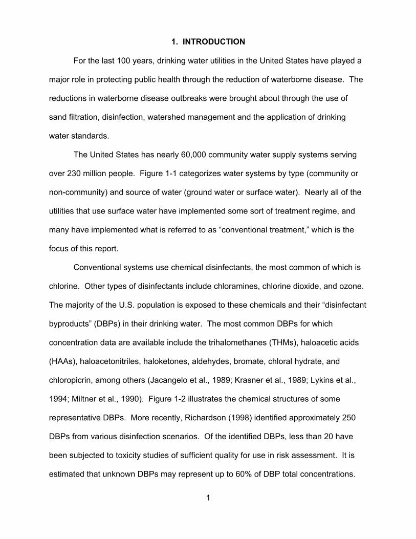
1. INTRODUCTION
For the last 100 years, drinking water utilities in the United States have played a
major role in protecting public health through the reduction of waterborne disease. The
reductions in waterborne disease outbreaks were brought about through the use of
sand filtration, disinfection, watershed management and the application of drinking
water standards.
The United States has nearly 60,000 community water supply systems serving
over 230 million people. Figure 1-1 categorizes water systems by type (community or
non-community) and source of water (ground water or surface water). Nearly all of the
utilities that use surface water have implemented some sort of treatment regime, and
many have implemented what is referred to as “conventional treatment,” which is the
focus of this report.
Conventional systems use chemical disinfectants, the most common of which is
chlorine. Other types of disinfectants include chloramines, chlorine dioxide, and ozone.
The majority of the U.S. population is exposed to these chemicals and their “disinfectant
byproducts” (DBPs) in their drinking water. The most common DBPs for which
concentration data are available include the trihalomethanes (THMs), haloacetic acids
(HAAs), haloacetonitriles, haloketones, aldehydes, bromate, chloral hydrate, and
chloropicrin, among others (Jacangelo et al., 1989; Krasner et al., 1989; Lykins et al.,
1994; Miltner et al., 1990). Figure 1-2 illustrates the chemical structures of some
representative DBPs. More recently, Richardson (1998) identified approximately 250
DBPs from various disinfection scenarios. Of the identified DBPs, less than 20 have
been subjected to toxicity studies of sufficient quality for use in risk assessment. It is
estimated that unknown DBPs may represent up to 60% of DBP total concentrations.
1
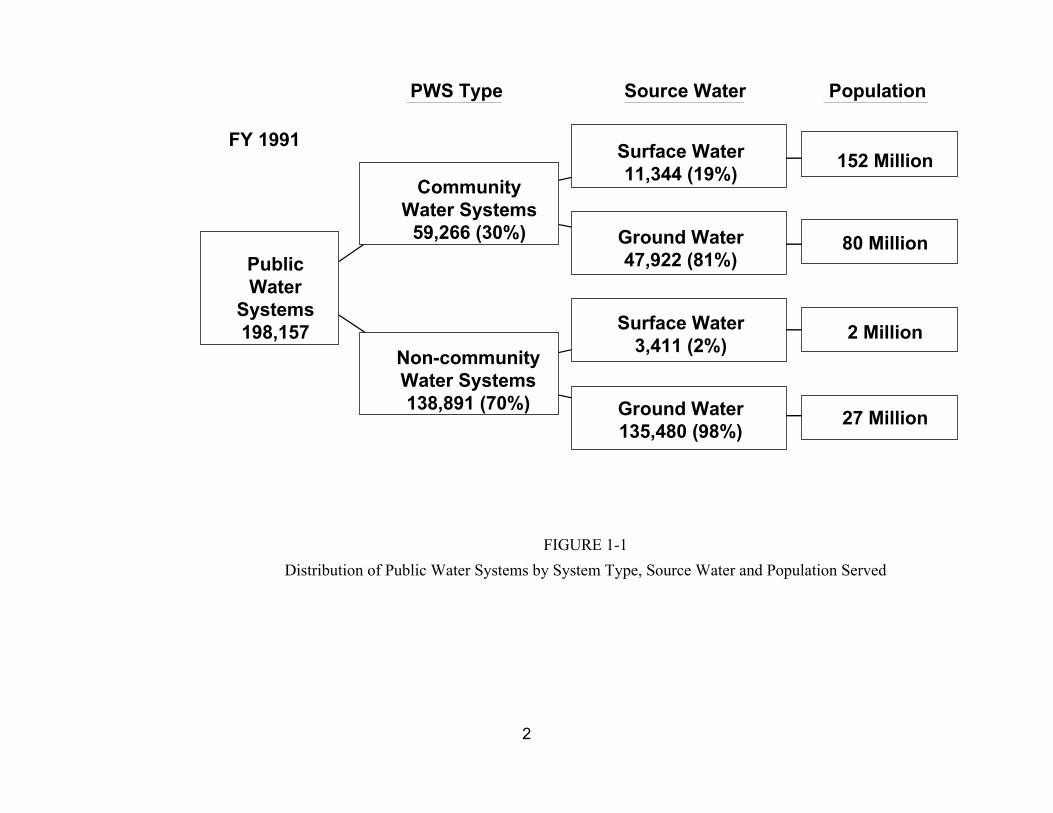
PWS Type Source Water Population
Public Water
Systems 198,157
Community Water Systems
59,266 (30%)
Non-community Water Systems 138,891 (70%)
Surface Water 11,344 (19%)
Ground Water 47,922 (81%)
Surface Water 3,411 (2%)
Ground Water 135,480 (98%)
152 Million
80 Million
2 Million
27 Million
FY 1991
FIGURE 1-1
Distribution of Public Water Systems by System Type, Source Water and Population Served
2

R
R C H
R
Trihalomethane
Cl
Cl C N O 2
Cl
Chloropicrin
R
R C
R
N C
Haloacetonitrile
Cl O H
Cl C C C H
Cl H
R O
R C C OH
R
Haloacetic Acid
Cl OH
Cl C C H
Cl OH
1,1,1-Trichloropropanone Chloral Hydrate
FIGURE 1-2
Representative Structures of DBPs
3
Data from both epidemiologic and toxicologic studies indicate that human health
effects from DBP exposure are of concern, but neither discipline has been able to
confirm this with confidence. DBPs typically occur at low levels in drinking water at
which general toxic effects from exposure to the environmental mixture have not been
found in animal studies (Bull et al., 1982; Kavlock et al., 1979). In contrast,
epidemiologic studies of chlorinated drinking water exposures in humans suggest weak
associations with bladder, rectal and colon cancer (Cantor et al., 1985; McGeehin et al.,
1993; King and Marrett, 1996; Cantor et al., 1997; Freedman et al. 1997) and limited
evidence of reproductive and developmental effects (Bove et al., 1995; Kramer et al.,
1992; Swan et al., 1998; Waller et al., 1998). Although there are few studies available
on defined mixtures of DBPs, evidence exists of dose-additivity for liver effects in mice
exposed to mixtures of trihalomethanes (THMs) (Gennings et al., 1997; U.S. EPA,
1998d) and of synergistic activity by mixtures of dichloroacetic acid (DCA) and
trichloroacetic acid (TCA) for promotion of cancer (Pereira et al., 1997). The majority of
the available DBP toxicity data consists of single chemical in vivo or in vitro studies.
There is evidence in single chemical animal studies at high DBP dose levels of
carcinogenicity, reproductive effects, developmental effects, and other toxic effects,
particularly in the kidney and liver (Bull and Kopfler, 1991; NTP, 1985; 1986; 1989;
Smith et al., 1989). Finally, there is evidence of mutagenicity from exposure to extracts
of finished drinking water in in vitro studies (Kool et al., 1981; Loper et al., 1978;
Nestmann et al., 1982).
This report discusses a risk assessment for DBPs in drinking water based on
work conducted as part of NCEA Cincinnati’s Comparative Risk Framework
Methodology (CRFM) project (U.S. EPA, 1998). The risk assessment evaluates two
4
alternative drinking water disinfection strategies, illustrated in Figure 1-3. The top
branch in Figure 1-3 illustrates the so-called “filter-chlorine” treatment train. Here,
treatment consists of:
• Coagulation / Rapid Mix – Enhances the precipitation of contaminants out of the water
• Flocculation – Further promotes precipitation of contaminants;
• Sedimentation / Clarification – Further filters particulate matter out of the drinking water;
• Filtration – Removes material from drinking water by passing it through a porous medium;
• Disinfection – Adds chemicals to the water to kill or inactivate common microorganisms.
The bottom branch in Figure 1-3 illustrates the “ozone-filter-chlorine” treatment train.
This treatment train augments the “filter-chlorine” treatment train (top branch) by
inserting a pre-ozonation step prior to coagulation / rapid mix. Ozone is a strong
disinfectant, and can also oxidize some DBP precursors, hence depressing their
formation.
The remainder of this document consists of 4 sections. Section 2 provides an
overview of the methodology used for this risk assessment. This methodology uses
Monte Carlo simulation to quantify the impact of uncertainty and variability (population
heterogeneity) on estimates of risk. Because Monte Carlo analysis is best suited to
address sources of uncertainty that can be characterized in terms of probability
distributions (so-called “parametric” uncertainty), the methodology also describes how
other sources of uncertainty are addressed outside of the simulation, including so-called
“model uncertainty” and “dataset uncertainty,” discussed below.
5
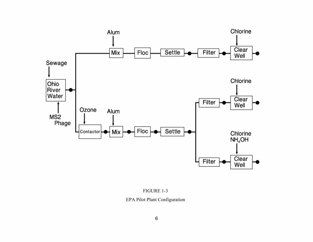
FIGURE 1-3
EPA Pilot Plant Configuration
6
Section 3 quantifies DBP exposure, presenting estimates of both DBP
concentrations in drinking water, and drinking water consumption rate estimates.
Section 4 discusses DBP toxicity (carcinogenic, developmental, and reproductive
effects). Information discussed in Section 4 includes the use of animal study data,
epidemiological results, and toxicity estimates inferred using Quantitative Structural
Activity Relationship (QSAR) modeling.
Finally, Section 5 of this report describes the results of this risk assessment.
Note that Sections 3.1, 3.2, and 4 begin with a summary of the parameter
estimates used in this risk assessment, along with their “parametric” uncertainty. These
summaries also identify potential sources of “model uncertainty” and “dataset
uncertainty.” Model uncertainty is introduced when there is more than one plausible
mathematical formulation describing some quantity. Dataset uncertainty is introduced
when there is more than one data set that can be used to quantify a parameter, and the
datasets cannot be directly combined. The results section of this risk assessment
investigates the potential implications of the sources of model uncertainty and dataset
uncertainty identified in Sections 3 and 4, specifying which of these sources of
uncertainty must be resolved in order to quantify risks with an acceptable level of
confidence.
7
2. METHODOLOGY
This section first presents the basic risk equation used in this risk assessment
(Section 2.1). Section 2.2 then discusses the distinction between uncertainty and
variability and how the Monte Carlo simulation is used to model the impact of these
stochastic characteristics on risk. Section 2.3 describes how the results of the Monte
Carlo analysis are used to identify which sources of parametric uncertainty (uncertainty
that can be characterized as a probability distribution for a parameter) have the greatest
influence on the results. Finally, Section 2.4 describes how this risk assessment
addresses sources of uncertainty that cannot be readily characterized parametrically,
including model uncertainty and data set uncertainty.
2.1. THE RISK EQUATION
This risk assessment estimates the risk associated with exposure to drinking
water treated using either of two drinking water disinfection technologies (filter-chlorine
referred to as “filter-Cl” and ozone-filter-chlorine, referred to as “O3-filter-Cl”), as
discussed in Section 1. As explained in Section 4, the risk posed by each DBP is
assumed to be a linear function of intake. Therefore, the risk posed by each DBP
equals the product of three quantities: 1) Tap water intake (Y L/day), 2) the DBP’s
concentration in tap water (C :g/L), and 3) the incremental risk per mg/kg-day DBP
intake (S per mg/kg-day). Section 4 explains the underlying mixtures risk assessment
methodology, which employs the response addition approach. Based on response
addition, the incremental risk to an individual due to drinking water exposure is the sum
of the risks over all the DBPs multiplied by a conversion constant of 1 mg / 1,000 :g.
This risk is therefore,
8
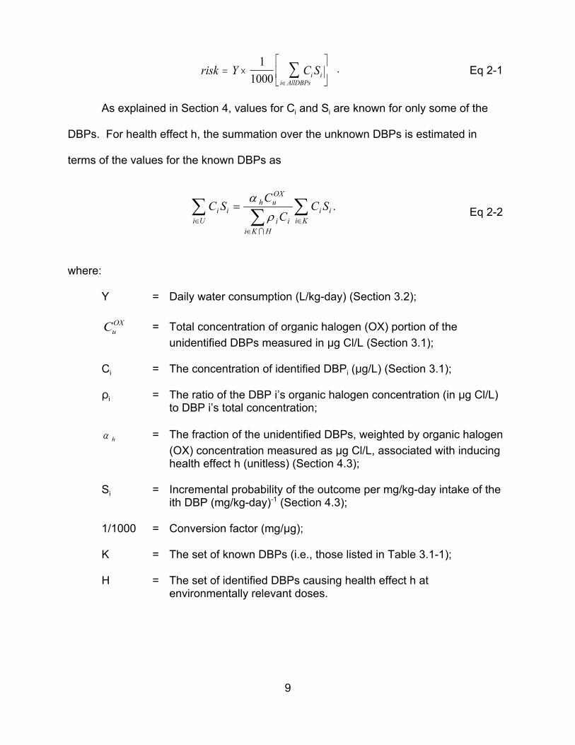
risk = Y × 1 ∑ C S
. Eq 2-11000
i∈AllDBPs
i i
As explained in Section 4, values for Ci and Si are known for only some of the
DBPs. For health effect h, the summation over the unknown DBPs is estimated in
terms of the values for the known DBPs as
∑ C S =α hCu
OX
∑ C S . Eq 2-2i i i i ∈ ∈i U ∑ρ iCi i K
i K I H∈
where:
Y = Daily water consumption (L/kg-day) (Section 3.2);
CuOX = Total concentration of organic halogen (OX) portion of the
unidentified DBPs measured in :g Cl/L (Section 3.1);
Ci = The concentration of identified DBPi (:g/L) (Section 3.1);
Di = The ratio of the DBP i’s organic halogen concentration (in :g Cl/L) to DBP i’s total concentration;
α h = The fraction of the unidentified DBPs, weighted by organic halogen (OX) concentration measured as :g Cl/L, associated with inducing health effect h (unitless) (Section 4.3);
Si = Incremental probability of the outcome per mg/kg-day intake of the ith DBP (mg/kg-day)-1 (Section 4.3);
1/1000 = Conversion factor (mg/:g);
K = The set of known DBPs (i.e., those listed in Table 3.1-1);
H = The set of identified DBPs causing health effect h at environmentally relevant doses.
9
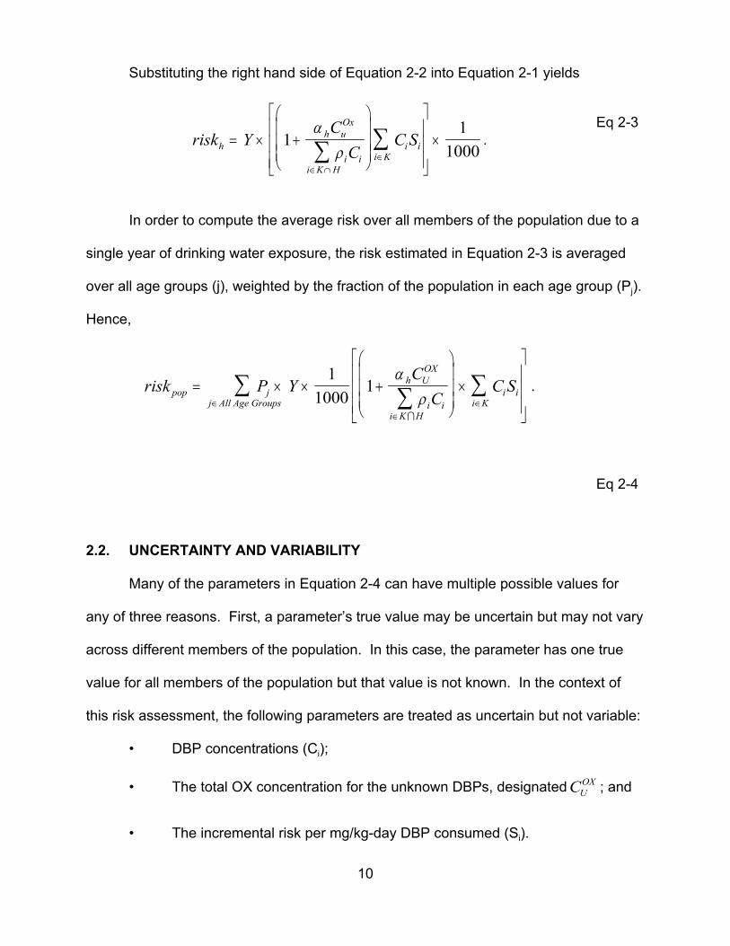
i K
Substituting the right hand side of Equation 2-2 into Equation 2-1 yields
α COx ∑ C S
1 Eq 2-3h uriskh = Y ×
1+ ∑ ρ C i K i i ×
1000 .
∈ ∩ Hi i ∈
In order to compute the average risk over all members of the population due to a
single year of drinking water exposure, the risk estimated in Equation 2-3 is averaged
over all age groups (j), weighted by the fraction of the population in each age group (Pj).
Hence,
α COX
risk pop = ∑ Pj × Y × 1000
h U
i i i K
i i
.
1 1+ ∑ ρ C
× ∑ C S
j∈All Age Groups ∈
i K I H∈
Eq 2-4
2.2. UNCERTAINTY AND VARIABILITY
Many of the parameters in Equation 2-4 can have multiple possible values for
any of three reasons. First, a parameter’s true value may be uncertain but may not vary
across different members of the population. In this case, the parameter has one true
value for all members of the population but that value is not known. In the context of
this risk assessment, the following parameters are treated as uncertain but not variable:
• DBP concentrations (Ci);
OX ; and• The total OX concentration for the unknown DBPs, designated CU
• The incremental risk per mg/kg-day DBP consumed (Si).
10

It may be that some of these quantities (such as the Si parameters) do vary from
member to member of the population because of, for example, differences in sensitivity.
However, since these differences cannot be observed in any individual, they are omitted
from the analysis.
Second, a parameter’s value may vary from member to member of the
population but be treated as known with certainty. In this risk assessment, drinking
water intake rates are put into this category. Note that while it is of course true that
these values are not perfectly known, they are thought to be known well enough that
quantitative characterization of their uncertainty would not appreciably alter the results
of this analysis.
Finally, a quantity may both be uncertain and vary from member to member of
the population. For this risk assessment, there are no quantities that fall into this
category.
It is important to segregate the influence of uncertainty and variability because
they give rise to two different sets of questions. Uncertainty raises the question of how
precise the resulting risk estimates are, whereas variability raises the question of
whether there are (identifiable) members of the population at a particularly elevated risk.
This risk assessment uses a technique known as “two-dimensional” or “two-
phase” Monte Carlo analysis to separately characterize the influence of uncertainty and
population variability on estimated risk. A “one-dimensional” or “one-phase” Monte
Carlo works by repeatedly drawing randomly selected values for each stochastic
parameter (a parameter that either varies from person to person or is uncertain). For
each set of values drawn, the simulation computes a risk, repeating this process a large
number of times (typically 1,000 to 10,000 times). The resulting set of risk estimates
11

can be plotted as a histogram that approximates the range and relative likelihood of the
plausible risks that may exist in the modeled population. This approximation to the
probability distribution of risks generated by a one-phase Monte Carlo simulation has
embedded within it both variability and uncertainty. Because it reflects both uncertainty
and variability, it is broader than the true distribution of risks. Moreover, it cannot be
thought of as representing the risk that any one individual would incur.
The two-phase simulation addresses this problem by conducting a large number
of separate one-phase simulations. For each one-phase simulation, a fixed set of
randomly selected values are assigned to each of the uncertain parameters. However,
values for variable parameters are permitted to vary within each one-phase simulation.
Hence each one-phase simulation, which produces a large number of risk estimates (in
the case of this risk assessment, 1,000 such estimates), represents the set of risks
incurred by members of a population, given the assumptions embedded in the fixed
values assigned to each uncertain parameter for the duration of that simulation. For this
risk assessment, a total of 1,000 one-phase simulations were executed. In practice, the
two-dimensional simulation is executed as illustrated in Figure 2-1.
The results of the analysis can be used to quantify the distribution of plausible
risks for representative members of the population. For example, the range of plausible
risks for the “median individual” (i.e., the individual whose risk is greater than the risk for
one-half of the population, and less than the risk for the other half) is estimated by
collecting the median risk values generated by each of the 1,000 executed one-phase
simulations.
12
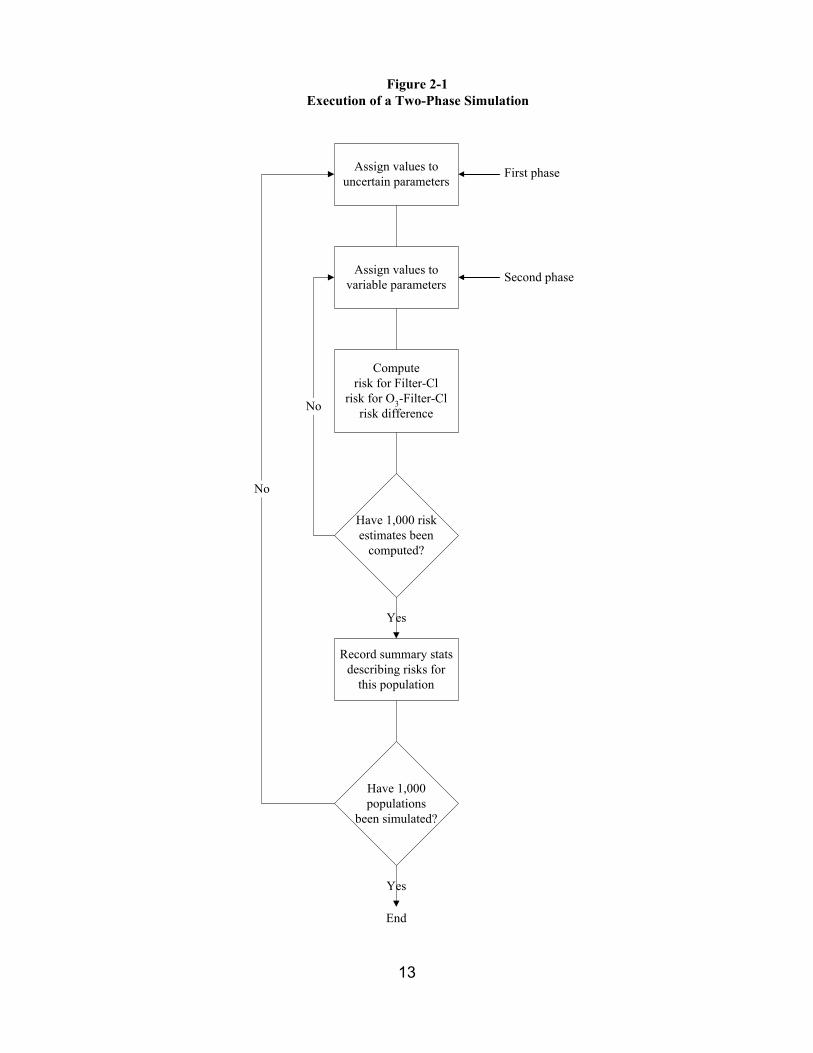
Figure 2-1Execution of a Two-Phase Simulation
Assign values to uncertain parameters
Assign values to variable parameters
Compute risk for Filter-Cl
risk for O3-Filter-Cl risk difference
Record summary stats describing risks for
this population
Have 1,000 risk estimates been
computed?
Have 1,000 populations
been simulated?
No
No
Yes
Yes
First phase
Second phase
End
13
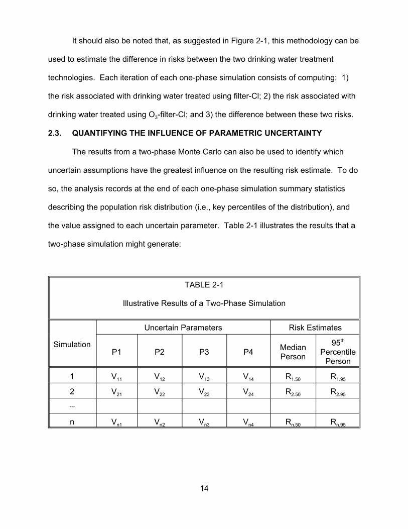
It should also be noted that, as suggested in Figure 2-1, this methodology can be
used to estimate the difference in risks between the two drinking water treatment
technologies. Each iteration of each one-phase simulation consists of computing: 1)
the risk associated with drinking water treated using filter-Cl; 2) the risk associated with
drinking water treated using O3-filter-Cl; and 3) the difference between these two risks.
2.3. QUANTIFYING THE INFLUENCE OF PARAMETRIC UNCERTAINTY
The results from a two-phase Monte Carlo can also be used to identify which
uncertain assumptions have the greatest influence on the resulting risk estimate. To do
so, the analysis records at the end of each one-phase simulation summary statistics
describing the population risk distribution (i.e., key percentiles of the distribution), and
the value assigned to each uncertain parameter. Table 2-1 illustrates the results that a
two-phase simulation might generate:
TABLE 2-1
Illustrative Results of a Two-Phase Simulation
Simulation
Uncertain Parameters Risk Estimates
P1 P2 P3 P4 Median Person
95th
Percentile Person
1 V11 V12 V13 V14 R1.50 R1.95
2 21 V22 V23 V24 R2.50 R2.95
@@@
n n1 Vn2 Vn3 Vn4 Rn.50 Rn.95
V
V
14
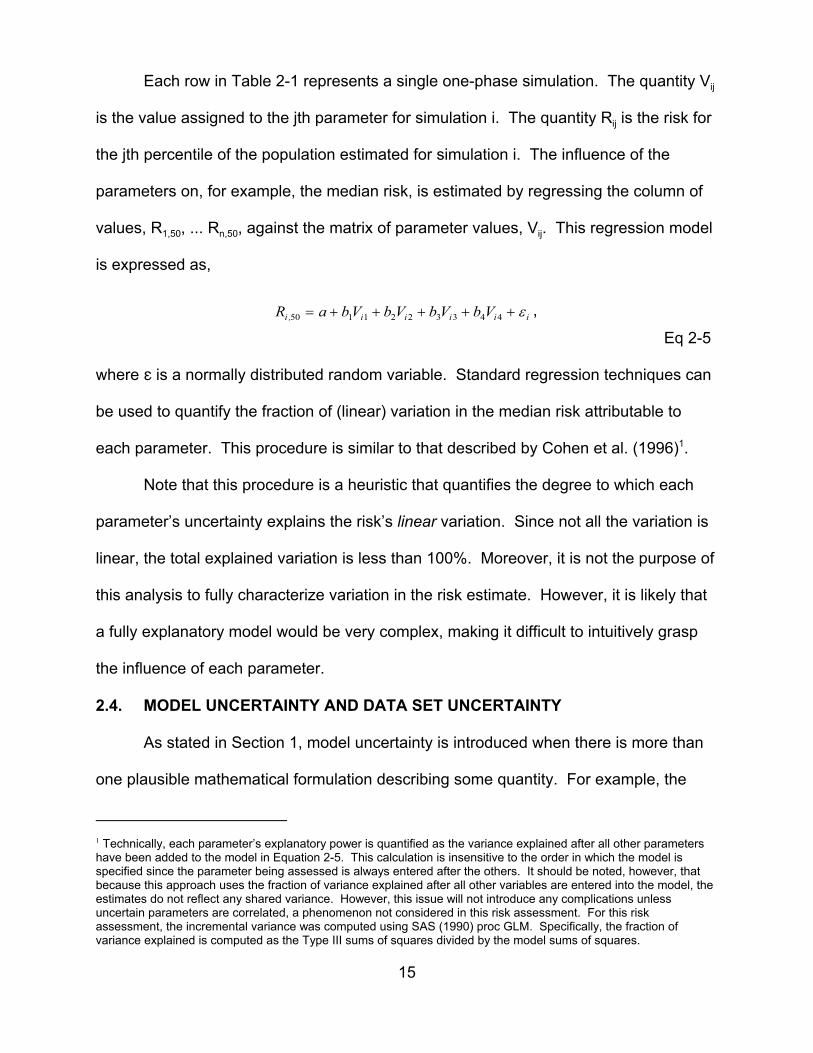
Each row in Table 2-1 represents a single one-phase simulation. The quantity Vij
is the value assigned to the jth parameter for simulation i. The quantity Rij is the risk for
the jth percentile of the population estimated for simulation i. The influence of the
parameters on, for example, the median risk, is estimated by regressing the column of
values, R1,50, ... Rn,50, against the matrix of parameter values, Vij. This regression model
is expressed as,
Ri ,50 = a + b1Vi1 + b Vi 2 + b3Vi3 + b Vi4 + ε i ,2 4
Eq 2-5
where g is a normally distributed random variable. Standard regression techniques can
be used to quantify the fraction of (linear) variation in the median risk attributable to
each parameter. This procedure is similar to that described by Cohen et al. (1996)1.
Note that this procedure is a heuristic that quantifies the degree to which each
parameter’s uncertainty explains the risk’s linear variation. Since not all the variation is
linear, the total explained variation is less than 100%. Moreover, it is not the purpose of
this analysis to fully characterize variation in the risk estimate. However, it is likely that
a fully explanatory model would be very complex, making it difficult to intuitively grasp
the influence of each parameter.
2.4. MODEL UNCERTAINTY AND DATA SET UNCERTAINTY
As stated in Section 1, model uncertainty is introduced when there is more than
one plausible mathematical formulation describing some quantity. For example, the
1 Technically, each parameter’s explanatory power is quantified as the variance explained after all other parameters have been added to the model in Equation 2-5. This calculation is insensitive to the order in which the model is specified since the parameter being assessed is always entered after the others. It should be noted, however, that because this approach uses the fraction of variance explained after all other variables are entered into the model, the estimates do not reflect any shared variance. However, this issue will not introduce any complications unless uncertain parameters are correlated, a phenomenon not considered in this risk assessment. For this risk assessment, the incremental variance was computed using SAS (1990) proc GLM. Specifically, the fraction of variance explained is computed as the Type III sums of squares divided by the model sums of squares.
15
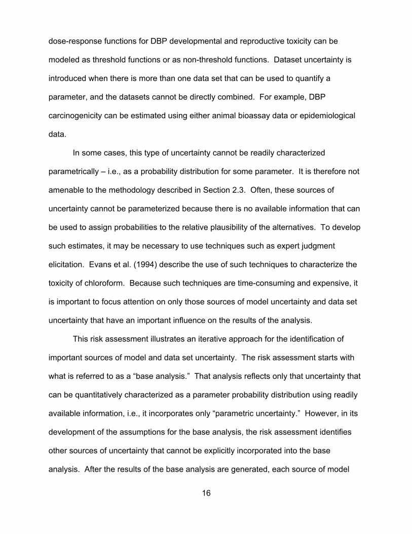
dose-response functions for DBP developmental and reproductive toxicity can be
modeled as threshold functions or as non-threshold functions. Dataset uncertainty is
introduced when there is more than one data set that can be used to quantify a
parameter, and the datasets cannot be directly combined. For example, DBP
carcinogenicity can be estimated using either animal bioassay data or epidemiological
data.
In some cases, this type of uncertainty cannot be readily characterized
parametrically – i.e., as a probability distribution for some parameter. It is therefore not
amenable to the methodology described in Section 2.3. Often, these sources of
uncertainty cannot be parameterized because there is no available information that can
be used to assign probabilities to the relative plausibility of the alternatives. To develop
such estimates, it may be necessary to use techniques such as expert judgment
elicitation. Evans et al. (1994) describe the use of such techniques to characterize the
toxicity of chloroform. Because such techniques are time-consuming and expensive, it
is important to focus attention on only those sources of model uncertainty and data set
uncertainty that have an important influence on the results of the analysis.
This risk assessment illustrates an iterative approach for the identification of
important sources of model and data set uncertainty. The risk assessment starts with
what is referred to as a “base analysis.” That analysis reflects only that uncertainty that
can be quantitatively characterized as a parameter probability distribution using readily
available information, i.e., it incorporates only “parametric uncertainty.” However, in its
development of the assumptions for the base analysis, the risk assessment identifies
other sources of uncertainty that cannot be explicitly incorporated into the base
analysis. After the results of the base analysis are generated, each source of model
16

uncertainty and data set uncertainty flagged earlier are revisited, and their potential
influence on the results is estimated. Those sources of uncertainty whose potential
influence is great are candidates for further investigation. If their influence is great
enough, it may be warranted to conclude that until further investigation is conducted, the
results of the risk assessment lack adequate precision. Of course, what level of
precision is adequate depends on what the results will be used for.
If further information is collected to address the most influential sources of model
uncertainty, it may become possible to explicitly incorporate into the risk assessment
sources of uncertainty that previously could not be characterized parametrically. The
process can then be repeated to determine if any additional sources of uncertainty must
be investigated before the results of the risk assessment warrant an acceptable level of
confidence.
17
3. EXPOSURE TO DBPs
Section 3.1 quantifies the concentration of DBPs in tap water, while Section 3.2
quantifies tap water intake.
3.1. DBP CONCENTRATIONS IN DRINKING WATER
With the exception of bromate, this risk assessment uses the results reported by
Miltner et al. (1990) to quantify DBP concentrations. Section 3.1.1 discusses the
concentration of identified DBPs reported by Miltner et al., and Section 3.1.2 discusses
the use of the Miltner et al. results to quantify those DBPs not individually identified in
terms of their collective total organic halogen (OX) concentration measured in terms of
:g Cl/L. Because the toxicity calculations in Section 4 require a comparison of the
known and unknown DBP concentrations, it was also necessary to quantify the OX
concentration value for each identified DBP (in terms of :g Cl/L). Section 3.1.3
discusses results from Miltner et al. (1992) used to quantify bromate concentrations.
Table 3-1 summarizes the assumed concentration distributions used here for “known”
DBPs identified by Miltner et al. (1990, 1992). Note that in all cases, it is assumed that
the distributions describing the concentration of each DBP is normal.
There are no appreciable sources of uncertainty that cannot be quantitatively
parameterized. In the case of the identified DBPs, there is no reason to believe that the
concentration measurements are substantially in error, although they have been
compared only to measurements from a pilot treatment plant and simulated distribution
system. For the unidentified DBPs, there is no reason to believe that the calculated OX
concentration is substantially in error. However, as with the identified DBPs, these
measurements are based on data from a pilot treatment plant and simulated distribution
system.
18
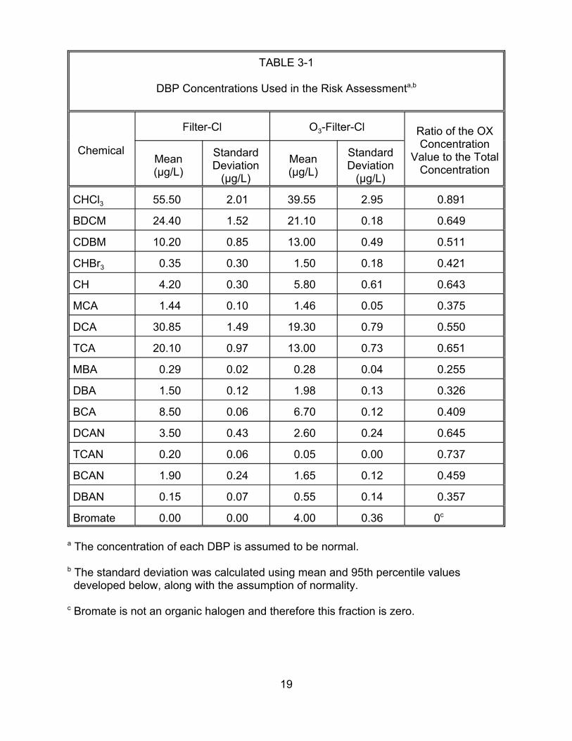
TABLE 3-1
DBP Concentrations Used in the Risk Assessmenta,b
Filter-Cl O3-Filter-Cl Ratio of the OX ConcentrationChemical
Mean (µg/L)
Standard Deviation
(µg/L)
Mean (µg/L)
Standard Deviation
(µg/L)
CHCl3 55.50 2.01 39.55 2.95
BDCM 24.40 1.52 21.10 0.18
CDBM 10.20 0.85 13.00 0.49
CHBr3 0.35 0.30 1.50 0.18
CH 4.20 0.30 5.80 0.61
MCA 1.44 0.10 1.46 0.05
DCA 30.85 1.49 19.30 0.79
TCA 20.10 0.97 13.00 0.73
MBA 0.29 0.02 0.28 0.04
DBA 1.50 0.12 1.98 0.13
BCA 8.50 0.06 6.70 0.12
DCAN 3.50 0.43 2.60 0.24
TCAN 0.20 0.06 0.05 0.00
BCAN 1.90 0.24 1.65 0.12
DBAN 0.15 0.07 0.55 0.14
Bromate 0.00 0.00 4.00 0.36
a The concentration of each DBP is assumed to be normal.
Value to the Total Concentration
0.891
0.649
0.511
0.421
0.643
0.375
0.550
0.651
0.255
0.326
0.409
0.645
0.737
0.459
0.357
0c
b The standard deviation was calculated using mean and 95th percentile values developed below, along with the assumption of normality.
c Bromate is not an organic halogen and therefore this fraction is zero.
19
3.1.1. Identified DBPs (Excluding Bromate). EPA has performed a series of studies
in its pilot water treatment plant in Cincinnati, Ohio to quantify the impact of chemical
disinfectants on DBP concentrations. Miltner et al. (1990) describe the plant and its
operation descriptions in detail (see Appendix A). For this study, raw Ohio River water
was trucked to the U.S. EPA and treated at 1.7 gpm. For the O3-filter-Cl treatment train,
ozone was applied so that the transferred ozone/TOC (total organic carbon) ratio was
approximately 80%. Chlorine was applied in the clear well after filtration to yield a free
residual near 0.2 mg/L in samples taken from the clear wells and stored for 3 days to
simulate distribution. Chlorine doses were in the range of 2.8 to 3.0 mg/L, resulting in
free chlorine residuals in clear well effluents near 1.2 mg/L. Detention time in the clear
wells was approximately 9.5 hours.
The mean and 95th percentile values listed in Table 3-2 were developed from
data provided by Miltner et al. (1990). Note that these statistics differ slightly from the
distributions published by Miltner et al. (1990) because this risk assessment
recalculated the means and confidence limits assuming a normal distribution and
substituting half the detection limit for non-detects in the Miltner et al. data rather than
replacing non-detects with zero, as in the original publication.
3.1.2. Unidentified TOX. The OX concentration for the unidentified DBPs ( CU OX ) was
calculated as
Eq 3-1 Cu
OX = CTOX − ∑ ρ C ,i i
i K∈
20
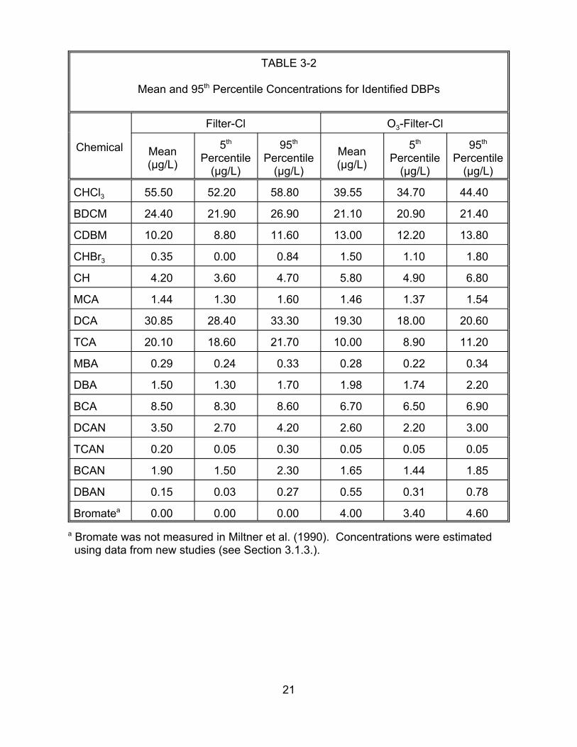
TABLE 3-2
Mean and 95th Percentile Concentrations for Identified DBPs
Chemical
Filter-Cl O3-Filter-Cl
Mean (µg/L)
5th
Percentile (µg/L)
95th
Percentile (µg/L)
Mean (µg/L)
5th
Percentile (µg/L)
95th
Percentile (µg/L)
CHCl3 55.50 52.20 58.80 39.55
BDCM 24.40 21.90 26.90
CDBM 10.20 8.80 11.60
CHBr3 0.35 0.00 0.84
CH 4.20 3.60 4.70
MCA 1.44 1.30 1.60
DCA 30.85 28.40 33.30
TCA 20.10 18.60 21.70
MBA 0.29 0.24 0.33
DBA 1.50 1.30 1.70
BCA 8.50 8.30 8.60
DCAN 3.50 2.70 4.20
TCAN 0.20 0.05 0.30
BCAN 1.90 1.50 2.30
DBAN 0.15 0.03 0.27
Bromatea 0.00 0.00 0.00
21.10
13.00
1.50
5.80
1.46
19.30
10.00
0.28
1.98
6.70
2.60
0.05
1.65
0.55
4.00
34.70
20.90
12.20
1.10
4.90
1.37
18.00
8.90
0.22
1.74
6.50
2.20
0.05
1.44
0.31
3.40
44.40
21.40
13.80
1.80
6.80
1.54
20.60
11.20
0.34
2.20
6.90
3.00
0.05
1.85
0.78
4.60 a Bromate was not measured in Miltner et al. (1990). Concentrations were estimated
using data from new studies (see Section 3.1.3.).
21
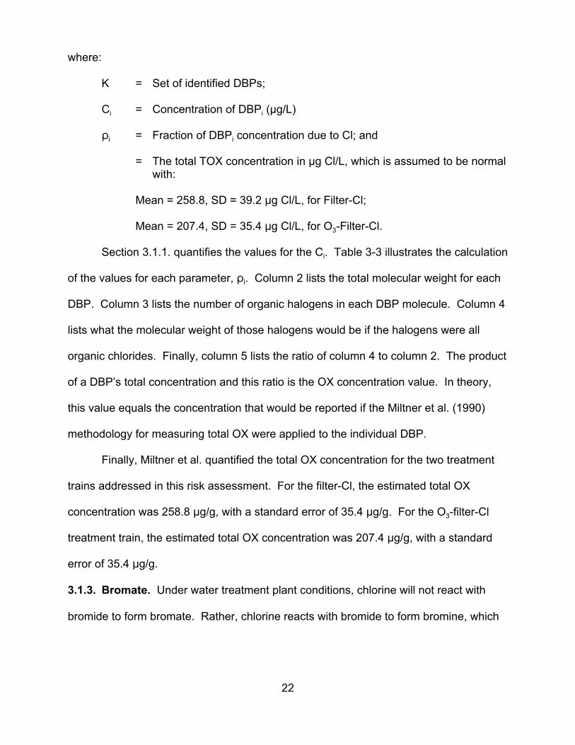
where:
K = Set of identified DBPs;
Ci = Concentration of DBPi (µg/L)
Di = Fraction of DBPi concentration due to Cl; and
= The total TOX concentration in µg Cl/L, which is assumed to be normal with:
Mean = 258.8, SD = 39.2 :g Cl/L, for Filter-Cl;
Mean = 207.4, SD = 35.4 :g Cl/L, for O3-Filter-Cl.
Section 3.1.1. quantifies the values for the Ci. Table 3-3 illustrates the calculation
of the values for each parameter, Di. Column 2 lists the total molecular weight for each
DBP. Column 3 lists the number of organic halogens in each DBP molecule. Column 4
lists what the molecular weight of those halogens would be if the halogens were all
organic chlorides. Finally, column 5 lists the ratio of column 4 to column 2. The product
of a DBP’s total concentration and this ratio is the OX concentration value. In theory,
this value equals the concentration that would be reported if the Miltner et al. (1990)
methodology for measuring total OX were applied to the individual DBP.
Finally, Miltner et al. quantified the total OX concentration for the two treatment
trains addressed in this risk assessment. For the filter-Cl, the estimated total OX
concentration was 258.8 :g/g, with a standard error of 35.4 :g/g. For the O3-filter-Cl
treatment train, the estimated total OX concentration was 207.4 :g/g, with a standard
error of 35.4 :g/g.
3.1.3. Bromate. Under water treatment plant conditions, chlorine will not react with
bromide to form bromate. Rather, chlorine reacts with bromide to form bromine, which
22
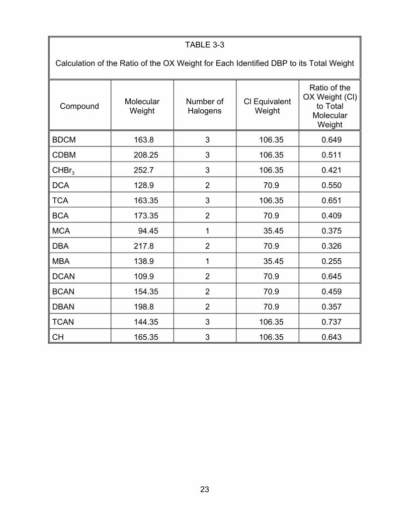
TABLE 3-3
Calculation of the Ratio of the OX Weight for Each Identified DBP to its Total Weight
Compound Molecular Weight
Number ofHalogens
BDCM 163.8 3
CDBM 208.25 3
CHBr3 252.7 3
DCA 128.9 2
TCA 163.35 3
BCA 173.35 2
MCA 94.45 1
DBA 217.8 2
MBA 138.9 1
DCAN 109.9 2
BCAN 154.35 2
DBAN 198.8 2
TCAN 144.35 3
CH 165.35 3
Cl Equivalent Weight
Ratio of the OX Weight (Cl)
to Total Molecular
Weight
106.35 0.649
106.35 0.511
106.35 0.421
70.9 0.550
106.35 0.651
70.9 0.409
35.45 0.375
70.9 0.326
35.45 0.255
70.9 0.645
70.9 0.459
70.9 0.357
106.35 0.737
106.35 0.643
23

reacts with organic compounds to form brominated DBPs. Hence, in the case of the
filter-Cl treatment train, the assumed bromate concentration is zero.
Data from Miltner et al. (1992) were used to estimate bromate levels generated
by the O3-filter-Cl treatment train. Transfer efficiencies, gas/liquid ratios, liquid depths,
ozone-to-TOC or DOC ratios, pHs, and temperatures were similar to the corresponding
conditions reported by Miltner et al. (1990). Miltner et al. (1992) reported an ambient
bromide concentration of 37 :g/L. At ozone/TOC ratios below 1 mg/mg, there was no
measurable bromate (when the bromate detection level was 7 :g/L). In Shukairy et al.
(1994), the ambient bromide concentration was 50.7 :g/L. At an ozone/TOC ratio near
0.8 mg/mg and a dissolved ozone residual near 0.6 mg/L, the bromate concentration
was near 4 :g/L. Thus, the estimate for bromate formation in this study would be near
4 :g/L, a level that is below the proposed MCL of 10 :g/L. Replication data described
in EPA Method 300.1 for bromate suggests that the expected deviation at 4 :g/L would
be ± 0.6 :g/L. Table 3-4 describes the basis for the estimate.
3.2. TAP WATER INTAKE
This risk assessment assumes that risks associated with exposure to tap water
depend on the quantity of tap water ingested daily. In the case of DBP-induced risks
(cancer, reproductive toxicity, and developmental toxicity), it is assumed that risk is a
function of total tap water consumption measured in L/kg-day (see Section 3.2.1.). For
this risk assessment, tap water consumption has been quantified by fitting lognormal
distributions to age-specific intake data described in U.S. EPA’s Exposure Factors
Handbook (U.S. EPA, 1997). Table 3-5 summarizes the lognormal distributions used
here.
24
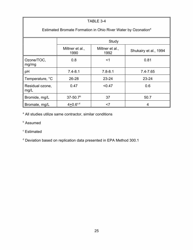
TABLE 3-4
Estimated Bromate Formation in Ohio River Water by Ozonationa
Study
Miltner et al., 1990
Miltner et al., 1992 Shukairy et al., 1994
Ozone/TOC, mg/mg
pH
Temperature, °C
Residual ozone, mg/L
Bromide, mg/L
Bromate, mg/L
0.81
7.4-8.1 7.8-8.1 7.4-7.65
26-28 23-24 23-24
0.47 <0.47 0.6
37-50.7b 37 50.7
4+0.6c,d <7 4
0.8 <1
a All studies utilize same contractor, similar conditions
b Assumed
c Estimated
d Deviation based on replication data presented in EPA Method 300.1
25
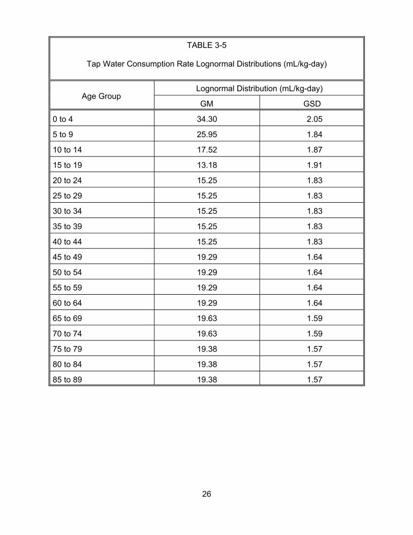
TABLE 3-5
Tap Water Consumption Rate Lognormal Distributions (mL/kg-day)
Age Group Lognormal Distribution (mL/kg-day)
GM GSD
0 to 4 34.30 2.05
5 to 9 25.95 1.84
10 to 14 17.52 1.87
15 to 19 13.18 1.91
20 to 24 15.25 1.83
25 to 29 15.25 1.83
30 to 34 15.25 1.83
35 to 39 15.25 1.83
40 to 44 15.25 1.83
45 to 49 19.29 1.64
50 to 54 19.29 1.64
55 to 59 19.29 1.64
60 to 64 19.29 1.64
65 to 69 19.63 1.59
70 to 74 19.63 1.59
75 to 79 19.38 1.57
80 to 84 19.38 1.57
85 to 89 19.38 1.57
26
Section 3.2.1. reviews the tap water consumption data used to derive these
estimates. Section 3.2.2. discusses potential differences in consumption among certain
subpopulations.
Sources of uncertainty that cannot be quantitatively parameterized include the
following (Section 3.2.3.):
• The assumption that ingestion dominates all other tap water intake pathways. Other pathways include inhalation and dermal absorption (e.g., while bathing).
• The assumption that total tap water ingestion is the relevant measure of intake (rather than, for example, unheated tap water intake).
Setting these issues aside, and assuming that ingestion is the only important
intake pathway, there do not appear to be any other notable sources of model
uncertainty or dataset uncertainty associated with the estimation of tap water intake
rates. It must be noted that the data on which these estimates are based was collected
more than a decade ago. Since that time, it is believed that some tap water
consumption has been replaced by the consumption of bottled water. Nonetheless, it is
unlikely that this shift has substantially altered total tap water consumption.
3.2.1. Tap Water Consumption Data. Table 3-6 in U.S. EPA’s Exposure Factors
Handbook (U.S. EPA, 1997) quantifies total tap water consumption in mL/kg-day for
individuals of all ages. Table 3-6 reproduces these rates for the 5th through 95th
percentiles of the population.
In order to standardize these data for use in the risk assessment, age-weighted
averages of these values have been computed to approximate consumption for age
groups defined in 5-year increments. The results appear in Table 3-7. The age-
weighted average for each 5-year interval was computed by weighting the values in
27
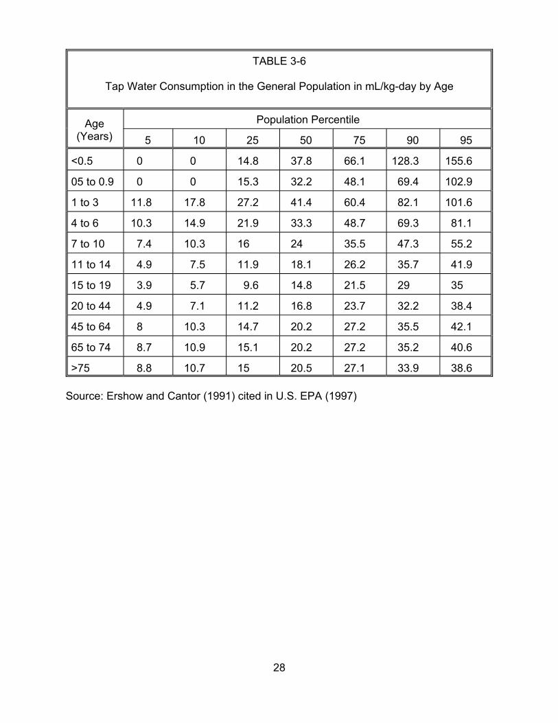
TABLE 3-6
Tap Water Consumption in the General Population in mL/kg-day by Age
Age (Years)
Population Percentile
5 10 5 0 5 0 5 2 5 7 9 9
<0.5 0 0 14.8 37.8 66.1 128.3 155.6
05 to 0.9 0 0 15.3 32.2 48.1 69.4 102.9
1 to 3 11.8 17.8 27.2 41.4 60.4 82.1 101.6
4 to 6 10.3 14.9 21.9 33.3 48.7 69.3 81.1
7 to 10 7.4 10.3 16 24 35.5 47.3 55.2
11 to 14 4.9 7.5 11.9 18.1 26.2 35.7 41.9
15 to 19 3.9 5.7 9.6 14.8 21.5 29 35
20 to 44 4.9 7.1 11.2 16.8 23.7 32.2 38.4
45 to 64 8 10.3 14.7 20.2 27.2 35.5 42.1
65 to 74 8.7 10.9 15.1 20.2 27.2 35.2 40.6
>75 8.8 10.7 15 20.5 27.1 33.9 38.6
Source: Ershow and Cantor (1991) cited in U.S. EPA (1997)
28

TABLE 3-7
Tap Water Consumption in the General Population in mL/kg-day by 5-Year Age Groupsa
Age (Years) Population Percentile
5 10 5 0 5 0 5 Arithmetic Meanb 2 5 7 9 9
91.4 13.66 23.71
5 to 9 8.56
10 to 14 5.4
15 to 19 3.9
20 to 24 4.9
25 to 29 4.9
30 to 34 4.9
35 to 39 4.9
40 to 44 4.9
45 to 49 8
50 to 54 8
55 to 59 8
60 to 64 8
65 to 69 8.7
70 to 74 8.7
75 to 79 8.8
80 to 84 8.8
85+ 8.8
12.14
8.06
5.7
7.1
7.1
7.1
7.1
7.1
10.3
10.3
10.3
10.3
10.9
10.9
10.7
10.7
10.7
18.36 27.72
12.72 19.28
9.6 14.8
11.2 16.8
11.2 16.8
11.2 16.8
11.2 16.8
11.2 16.8
14.7 20.2
14.7 20.2
14.7 20.2
14.7 20.2
15.1 20.2
15.1 20.2
15 20.5
15 20.5
15 20.5
0 to 4 38.5 57.4 82.89
40.78
28.06
21.5
23.7
23.7
23.7
23.7
23.7
27.2
27.2
27.2
27.2
27.2
27.2
27.1
27.1
27.1
56.1
38.02
29
32.2
32.2
32.2
32.2
32.2
35.5
35.5
35.5
35.5
35.2
35.2
33.9
33.9
33.9 38.6 21.4
103.03 44.4
65.56 31.2
44.56 21.3
35 16.3
38.4 18.3
38.4 18.3
38.4 18.3
38.4 18.3
38.4 18.3
42.1 21.8
42.1 21.8
42.1 21.8
42.1 21.8
40.6 21.9
40.6 21.9
38.6 21.4
38.6 21.4
a Source: Ershow and Cantor (1991) cited in U.S. EPA. 1997
b The arithmetic mean value for each age group was computed by fitting a lognormal to the percentile values listed and computing the arithmetic mean corresponding to that distribution’s geometric mean and geometric standard deviation.
29
Table 3-6 by duration contributed to that 5-year interval. Consider, for example, the
5-year interval between ages 5 and 9 (the second row of Table 3-7). The 4th row of
Table 3-6 (ages 4 to 6) contributes ages 5 and 6, or 40% of this duration, and the 5th
row (ages 7 to 10) contributes ages 7, 8, and 9, or 60% of this duration.
While these values reflect some sampling uncertainty, it is likely that, given the
nature of the survey on which it is based, the parametric uncertainty is not substantial.
3.2.2. Adjustments for Special Subgroups. No adjustments are made for subgroups.
3.2.2.1. The AIDS Subpopulation — Perz et al. (1998) report that members of
the AIDS subpopulation “may exhibit significant avoidance of tap water.” They estimate
that unheated tap water consumption among individuals in this subgroup is 70% of that
among members of the general population. Perz et al. (1998) do not state whether the
total tap water consumption rate for the AIDS subpopulation is also less than it is for the
general population. Here, it is assumed that no adjustment is necessary for this
population subgroup.
3.2.2.2. Pregnant Women — Because pregnant women are at risk for DBP-
induced reproductive health effects, and the fetus is at risk for DBP-induced
developmental effects, it is important to determine if pregnancy status affects tap water
consumption. Data quantifying tap water consumption rates for pregnant women are
limited. However, Ershow et al. (1991) report that the 50th percentile consumption rate
among pregnant women is 1.1 L/day, while the 90th percentile daily consumption rate is
2.2 L/day. These values are very close to the 50th and 90th percentile consumption
rates, respectively, for members of the general population, ages 20 to 44 years old, as
reported by U.S. EPA (1997a, Table 3-7). Those rates are 1.144 L/day and 2.121
L/day, respectively. The risk assessment therefore makes no adjustments to the tap
30
water consumption rate to reflect potential differences between pregnant women and
the general population.
3.2.3. Tap Water Intake — Model Uncertainty. Note that while it is not incorporated
into this risk assessment, it is possible that the inhalation pathway is a potential route of
exposure for the more volatile DBPs (e.g., Jo et al., 1990a,b provide estimates of
exposures to chloroform during showering). Because of a lack of data, this possibility is
not treated quantitatively in the risk assessment.
This risk assessment also assumes that the relevant measure of tap water intake
is total tap water ingestion. Total ingestion is used (rather than unheated tap water
consumption) because it is assumed that heating does not substantially affect DBP
concentrations. This assumption may lead to the slight overestimation of risk since it is
known that the more volatile DBPs, specifically, the trihalomethanes, will be removed by
heating. On the other hand, many other DBPs, such as the acids, will remain in the
water. Because of a lack of data specifically addressing the removal of these DBPs
from water by heating, this phenomenon is not treated quantitatively.
31
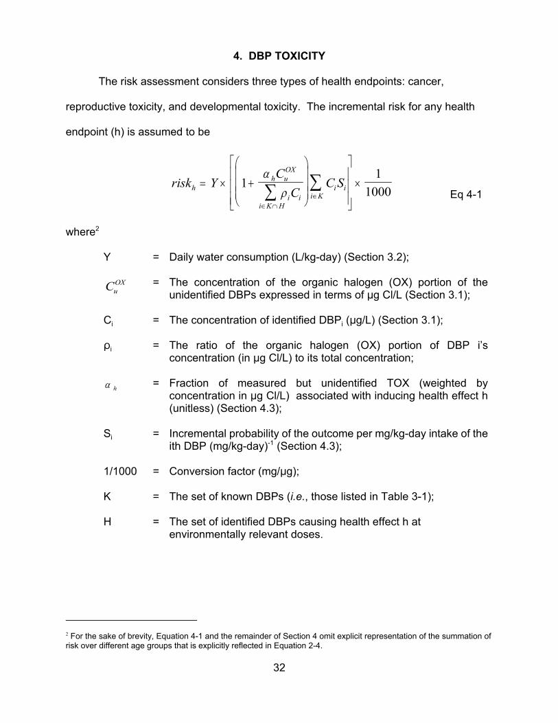
i K
4. DBP TOXICITY
The risk assessment considers three types of health endpoints: cancer,
reproductive toxicity, and developmental toxicity. The incremental risk for any health
endpoint (h) is assumed to be
α COX ∑ C S
1h uriskh = Y × 1+ ∑ ρ C i K
i i × 1000 Eq 4-1 ∈ ∩ H
i i ∈
where2
Y = Daily water consumption (L/kg-day) (Section 3.2);
CuOX = The concentration of the organic halogen (OX) portion of the
unidentified DBPs expressed in terms of :g Cl/L (Section 3.1);
Ci = The concentration of identified DBPi (:g/L) (Section 3.1);
Di = The ratio of the organic halogen (OX) portion of DBP i’s concentration (in :g Cl/L) to its total concentration;
α h = Fraction of measured but unidentified TOX (weighted by concentration in :g Cl/L) associated with inducing health effect h (unitless) (Section 4.3);
Si = Incremental probability of the outcome per mg/kg-day intake of the ith DBP (mg/kg-day)-1 (Section 4.3);
1/1000 = Conversion factor (mg/:g);
K = The set of known DBPs (i.e., those listed in Table 3-1);
H = The set of identified DBPs causing health effect h at environmentally relevant doses.
2 For the sake of brevity, Equation 4-1 and the remainder of Section 4 omit explicit representation of the summation of risk over different age groups that is explicitly reflected in Equation 2-4.
32
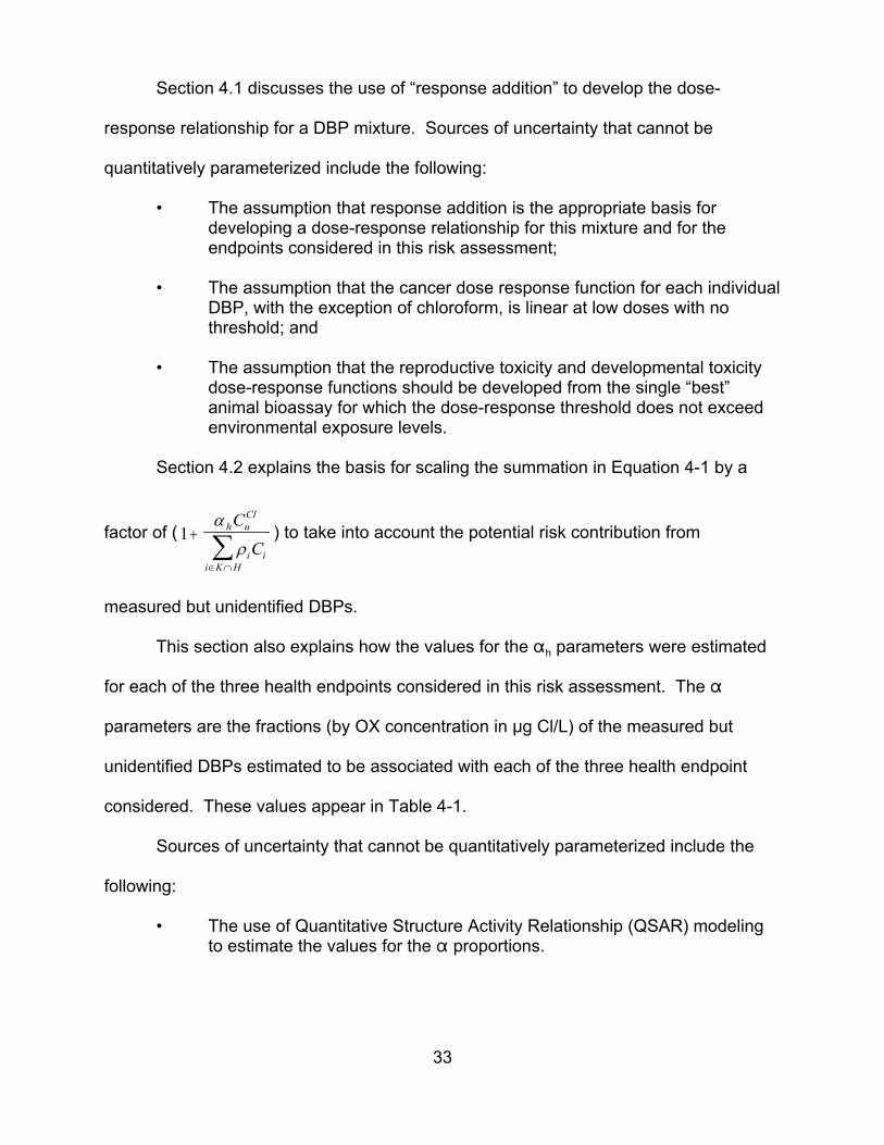
∈ ∩
Section 4.1 discusses the use of “response addition” to develop the dose-
response relationship for a DBP mixture. Sources of uncertainty that cannot be
quantitatively parameterized include the following:
• The assumption that response addition is the appropriate basis for developing a dose-response relationship for this mixture and for the endpoints considered in this risk assessment;
• The assumption that the cancer dose response function for each individual DBP, with the exception of chloroform, is linear at low doses with no threshold; and
• The assumption that the reproductive toxicity and developmental toxicity dose-response functions should be developed from the single “best” animal bioassay for which the dose-response threshold does not exceed environmental exposure levels.
Section 4.2 explains the basis for scaling the summation in Equation 4-1 by a
α CCl
factor of ( 1 + h u ) to take into account the potential risk contribution from∑ρ Ci i
i K H
measured but unidentified DBPs.
This section also explains how the values for the " h parameters were estimated
for each of the three health endpoints considered in this risk assessment. The "
parameters are the fractions (by OX concentration in :g Cl/L) of the measured but
unidentified DBPs estimated to be associated with each of the three health endpoint
considered. These values appear in Table 4-1.
Sources of uncertainty that cannot be quantitatively parameterized include the
following:
• The use of Quantitative Structure Activity Relationship (QSAR) modeling to estimate the values for the " proportions.
33
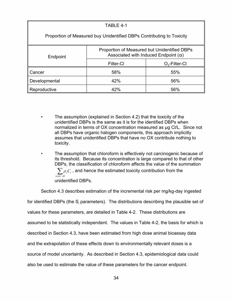
i K
TABLE 4-1
Proportion of Measured buy Unidentified DBPs Contributing to Toxicity
Endpoint Proportion of Measured but Unidentified DBPs
Associated with Induced Endpoint (")
Filter-Cl O3-Filter-Cl
Cancer 58% 55%
Developmental 42% 56%
Reproductive 42% 56%
• The assumption (explained in Section 4.2) that the toxicity of the unidentified DBPs is the same as it is for the identified DBPs when normalized in terms of OX concentration measured as :g Cl/L. Since not all DBPs have organic halogen components, this approach implicitly assumes that unidentified DBPs that have no OX contribute nothing to toxicity.
• The assumption that chloroform is effectively not carcinogenic because of its threshold. Because its concentration is large compared to that of other DBPs, the classification of chloroform affects the value of the summation
∑ρ C , and hence the estimated toxicity contribution from thei i ∈ ∩H
unidentified DBPs.
Section 4.3 describes estimation of the incremental risk per mg/kg-day ingested
for identified DBPs (the Si parameters). The distributions describing the plausible set of
values for these parameters, are detailed in Table 4-2. These distributions are
assumed to be statistically independent. The values in Table 4-2, the basis for which is
described in Section 4.3, have been estimated from high dose animal bioassay data
and the extrapolation of these effects down to environmentally relevant doses is a
source of model uncertainty. As described in Section 4.3, epidemiological data could
also be used to estimate the value of these parameters for the cancer endpoint.
34
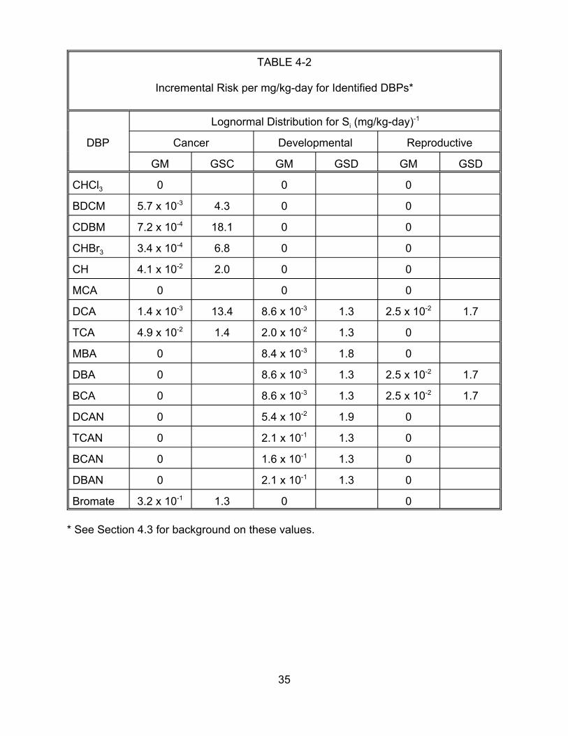
TABLE 4-2
Incremental Risk per mg/kg-day for Identified DBPs*
DBP
Lognormal Distribution for Si (mg/kg-day)-1
Cancer Developmental Reproductive
GM GSC GM GSD GM GSD
CHCl3 0 0 0
BDCM 5.7 x 10⁻³ 4.3 0 0
CDBM 7.2 x 10⁻⁴ 18.1 0 0
CHBr3 3.4 x 10⁻⁴ 6.8 0 0
CH 4.1 x 10⁻² 2.0 0 0
MCA 0
DCA 1.4 x 10⁻³ 13.4 8.6 x 10⁻³ 1.3 2.5 x 10⁻²
TCA 4.9 x 10⁻² 1.4 2.0 x 10⁻² 1.3 0
MBA 0 8.4 x 10⁻³ 1.8 0
DBA 0 8.6 x 10⁻³ 1.3 2.5 x 10⁻²
BCA 0 8.6 x 10⁻³ 1.3 2.5 x 10⁻²
DCAN 0 5.4 x 10⁻² 1.9 0
TCAN 0 2.1 x 10⁻¹ 1.3 0
BCAN 0 1.6 x 10⁻¹ 1.3 0
DBAN 0 2.1 x 10⁻¹ 1.3 0
Bromate 3.2 x 10⁻¹ 1.3 0 0
0 0
1.7
1.7
1.7
* See Section 4.3 for background on these values.
35

Sources of uncertainty that cannot be quantitatively parameterized include the
following:
• Reliance on animal bioassay data to quantify toxicity.
• The extrapolation from high doses used in animal bioassay experiments down to environmentally relevant doses.
• The assumption that these distributions are statistically independent. Making this assumption tends to decrease the range of plausible risk estimates for the DBP mixture as a whole.
4.1. RISK CHARACTERIZATION METHOD
4.1.1 Response Addition. This risk assessment uses “response addition” as the risk
characterization method for the mixture of DBPs in drinking water. Response addition
assumes only that the components of a mixture are functionally independent at low
doses so that the risks (i.e., the expected response) due to each can be added together
(Mumtaz and Hertzberg, 1993). Mathematically, the response addition assumption
translates into a dose response function of the form,
risk = ∑ ri , i∈All DBPs Eq 4-2
where ri is the risk contribution by DBPi at a given exposure.
The use of response addition as a risk characterization method is well
documented (U.S. EPA, 1986, 1989, 1990). It is particularly useful when the effects of
concern are thought to be present at low dose levels for each of the component
chemicals, even though they are highly unlikely to be observable at these low levels in
the environment; the mixture risk is then the sum of the individually low risks of the
independently acting component chemicals. The original U.S. EPA guidelines for
mixtures risk assessment (U.S. EPA, 1986) recommend a default no-interaction
36
approach of response addition for carcinogenic risk. Furthermore, there is strong
precedent for use of response addition for carcinogenic risk estimation as employed in
the evaluation of mixtures at Superfund sites (U.S. EPA 1989) and in assessments by
the Food and Drug Administration (Gaylor et al., 1997). Response-addition is less
commonly used for non-cancer endpoints because for many of these endpoints,
threshold effects are thought to exist; in this situation, dose-addition is a more common
assumption. (See Appendix B.1 for further discussion of alternative models.)
Response-addition is different from dose-addition in that it does not assume similar
kinetics or a similar mode of action and does not assume parallel dose-response curves
(Mumtaz and Hertzberg, 1993). Gaylor et al. (1997) state that,
“At dose levels far below those having measurable pharmacologic or physiologic activity, synergistic or antagonistic interactions are considered not to be likely. That is, it is assumed that the carcinogens are acting independently. Then, the risk of cancer from the mixtures may be obtained by summing the individual risks.”
The DBP mixtures response-addition assessment depends on the fact that we
are dealing with low level exposures. Thus, information on how these chemicals
interact at high dose levels is not pertinent to the risk assessment. The following text
from the newest Agency draft mixtures guidance document (U.S. EPA, 1998e)
describes the theoretical statistical basis for the response addition equation.
“Under response addition, the chemicals are assumed to behave independently of one another, so that the body’s response to the first chemical is the same whether or not the second chemical is present. In simplest terms, classical response addition is described by the statistical law of independent events, with “response” measured by the percentage of exposed animals that show toxicity. (Let r1 and r2 be risk estimates for chemicals 1 and 2, respectively, and let rm represent the risk for the mixture)....the statistical law of independence is:
37
rm = 1 - (1 - r1)*(1 - r2)
In terms of mixture response, this equation says that the response to either chemical 1 or 2 is one minus the probability of not responding to either chemical. Expanding the right-hand-side, one obtains:
rm = r1 + r2 - r1*r2
which, for small single chemical responses, is well approximated by the simple summation:
rm = r1 + r2”
Thus, this equation works well for DBP mixtures carcinogenic risk because 1) we
expect very small individual risks at the low levels of exposure (i.e., the ri are small) and
2) we do not expect to see interaction effects at these low doses (i.e., the interaction
term, r1*r2 can be ignored). For the developmental and reproductive endpoints, points
1) and 2) are also true. The dilemma is whether the individual ri values are actually
equal to zero due to threshold effects. Thus, response addition has been adopted as a
default approach, pending further research relative to the true biologic mechanisms for
these noncancer effects.
4.1.2. Low Dose Linearity and Calculation of the Incremental Risk per mg/kg-day.
With the exception of chloroform, the DBPs associated with carcinogenicity (see Section
4.3.1) are assumed to have dose-response functions that are linear at low dose.
For the noncancer health endpoints, it is assumed that there may be a threshold
at some nonzero dose. As described in Section 4.3.2, the dose-response functions
contributing to noncancer risk are effectively linear at low dose because the dose-
response curve fitting calculation in these cases failed to identify a threshold exceeding
zero.
38
× ×
Because all dose-response functions used in this risk assessment are effectively
1linear at low dose, the risk for endpoint h due to DBPi is 1000
Y Si × Ci . Summing
over the risks contributed by all DBPs yields
1risk = 1000 ∑Y × Si × Ci =
1 × Y × ∑ Si × Ci , Eq 4-3
i∈ All DBPs 1000 i∈ All DBPs
where:
Y = Daily water consumption (L/kg-day);
Ci = The concentration of identified DBPi (:g/L);
Si = Incremental probability of endpoint h per mg/kg-day intake of the ith DBP (mg/kg-day)-1; and
1/1000 = Conversion factor (mg/:g).
4.1.3. Chloroform’s Carcinogen Dose Response Threshold. The risk assessment
assumes that chloroform’s carcinogen dose-response function has a threshold, and that
as a result, it does not cause cancer at environmentally relevant exposure levels. This
assumption reflects the findings of a recent expert panel cancer assessment (U.S. EPA,
1998b) that employed methodology from EPA’s 1996 proposed Cancer Risk
Assessment Guidelines (U.S. EPA, 1996a). There is increasing evidence that the
carcinogenic mechanism of action for chloroform is not relevant at the low
concentrations found in drinking water and that, based on a margin of exposure (MOE)
assessment, any concentrations less than 300 :g/L of chloroform are not of concern for
human health. Thus, since the chloroform concentration for either treatment train
considered here is far below this level, EPA also assumed that chloroform does not
39
contribute to cancer risk. EPA also assumed that chloroform does not interact with
other components of the DBP mixture.
4.2. INCORPORATING MEASURED BUT UNIDENTIFIED DBPs
As noted in Section 3.1, Miltner et al. (1990) reported the total organic halogen
(total OX) concentrations in water processed by EPA’s Cincinnati pilot treatment plant.
For those chemicals contributing to total OX concentrations that are not identified, it is,
of course, not possible to assign chemical-specific dose-response functions. However,
omitting them entirely from this assessment would be equivalent to assuming that they
pose no toxicity risk at all. The toxicity of the unidentified DBPs (for cancer,
reproductive toxicity, and developmental toxicity) is assumed to be the same as it is for
identified DBPs when normalized in terms of OX concentration (:g Cl/L). That is, EPA
assumes that the incremental risk per :g OX/L (:g Cl/L) for the unidentified DPBs
equals the corresponding value for the identified DBPs.
While it may seem more natural to normalize in terms of total concentrations,
rather than in terms of OX concentrations, total concentration information is not
available for the unidentified DBPs. Normalization in terms of OX concentrations (:g
Cl/L) introduces a source of model uncertainty that cannot be readily quantified.
4.2.1. Dose Response Function Reflecting Unidentified DBPs. In order to quantify
the risk posed by the unidentified DBPs, the summation in Equation 4-3 is broken into
two parts – the first representing the risk contribution from identified DBPs, and the
second representing the risk contribution from the unidentified DBPs. Specifically,
1 Eq 4-4 risk =
1000 × Y ∑S C +∑S Ci i i i ,
i K i U ∈ ∈
40

where:
Y 0 Daily water consumption (L/kg-day);
Ci 0 The concentration of identified DBPi (:g/L);
Si 0 Incremental probability of endpoint h per mg/kg-day intake of the ith DBP (mg/kg-day)-1;
1/1000 0 Conversion factor (mg/:g).
K 0 The set of all “known” DBPs identified by Miltner et al.; and
U 0 The set of DBPs measured by Miltner et al. But not identified.
The values of the parameters in the summation over the set K can be determined
explicitly (see Section 3.1 for the value of the Ci parameters and Section 4.3 for the
value of the Si parameters). Of course, the value of the parameters in the second
summation are not known. It is instead assumed that for the fraction (by OX
concentration in :g Cl/L) of unidentified DBPs associated with inducing health endpoint
h (cancer, reproductive toxicity, or developmental toxicity), designated “" h”, the
incremental risk per :g Cl/L equals the corresponding value for the identified DBPs
associated with inducing endpoint h. If the total OX concentration for the unknown
DBPs is designated CuOX
, then the fraction associated with inducing endpoint h has a
total concentration of α h UCOX . The incremental risk per :g OX/L (in :g Cl/L) for the
unidentified DBPs is hence 1 × ×
1 ∑ C S . For the identified DBPs 1000
Y α hCu
OXi U
i i ∈
41
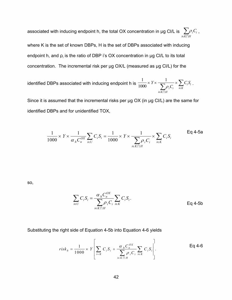
associated with inducing endpoint h, the total OX concentration in :g Cl/L is ∑ρ Ci i , i K I H∈
where K is the set of known DBPs, H is the set of DBPs associated with inducing
endpoint h, and Di is the ratio of DBP i’s OX concentration in :g Cl/L to its total
concentration. The incremental risk per :g OX/L (measured as :g Cl/L) for the
1 1 identified DBPs associated with inducing endpoint h is 1000
× ×∑ρ C
×∑C SY i i . ∈i i i K
∈i K I H
Since it is assumed that the incremental risks per :g OX (in :g Cl/L) are the same for
identified DBPs and for unidentified TOX,
1 × ×
1 ∑ C S = 1 1
i i
Eq 4-5a
1000 Y
α hCuOX
i U i i 1000
× Y × ∑ρ i Ci
×∑ C S ∈ i K∈
∈i K I H
so,
∑ C S =α hCu
OX
∑ C S .i i i i i U ∑ρ iCi i K Eq 4-5b∈ ∈
i K I H∈
Substituting the right side of Equation 4-5b into Equation 4-6 yields
1risk h =
1000 × Y
∑ C S
α h C uOX
∑ C S Eq 4-6
i i + ∑ ρ i C i i K
i i .
i K ∈=
i K I H ∈
42
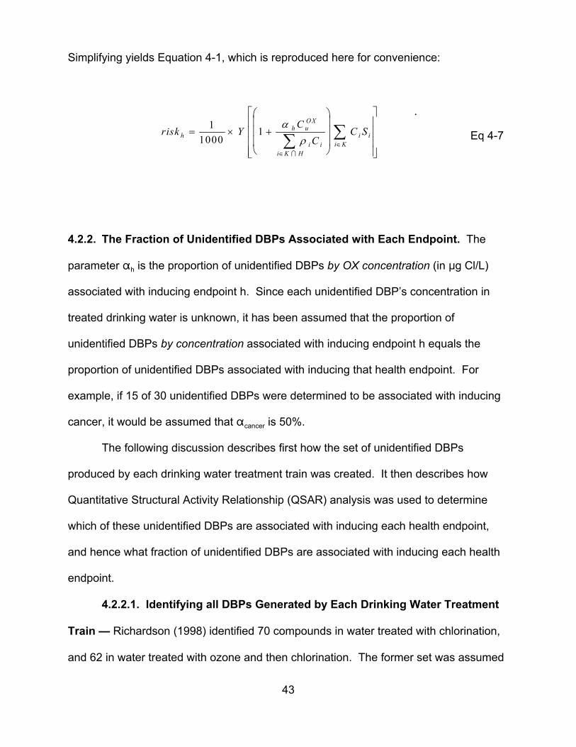
Simplifying yields Equation 4-1, which is reproduced here for convenience:
. 1risk h =
1000 × Y
1 +
α h C uOX
∑ C S
Eq 4-7 ∑ ρ i C i i K
i i ∈
i K I H ∈
4.2.2. The Fraction of Unidentified DBPs Associated with Each Endpoint. The
parameter " h is the proportion of unidentified DBPs by OX concentration (in :g Cl/L)
associated with inducing endpoint h. Since each unidentified DBP’s concentration in
treated drinking water is unknown, it has been assumed that the proportion of
unidentified DBPs by concentration associated with inducing endpoint h equals the
proportion of unidentified DBPs associated with inducing that health endpoint. For
example, if 15 of 30 unidentified DBPs were determined to be associated with inducing
cancer, it would be assumed that " cancer is 50%.
The following discussion describes first how the set of unidentified DBPs
produced by each drinking water treatment train was created. It then describes how
Quantitative Structural Activity Relationship (QSAR) analysis was used to determine
which of these unidentified DBPs are associated with inducing each health endpoint,
and hence what fraction of unidentified DBPs are associated with inducing each health
endpoint.
4.2.2.1. Identifying all DBPs Generated by Each Drinking Water Treatment
Train — Richardson (1998) identified 70 compounds in water treated with chlorination,
and 62 in water treated with ozone and then chlorination. The former set was assumed
43
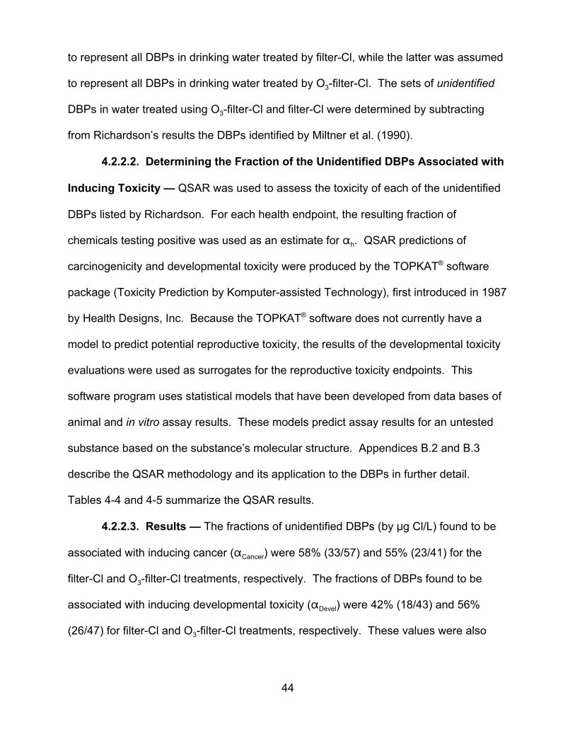
to represent all DBPs in drinking water treated by filter-Cl, while the latter was assumed
to represent all DBPs in drinking water treated by O3-filter-Cl. The sets of unidentified
DBPs in water treated using O3-filter-Cl and filter-Cl were determined by subtracting
from Richardson’s results the DBPs identified by Miltner et al. (1990).
4.2.2.2. Determining the Fraction of the Unidentified DBPs Associated with
Inducing Toxicity — QSAR was used to assess the toxicity of each of the unidentified
DBPs listed by Richardson. For each health endpoint, the resulting fraction of
chemicals testing positive was used as an estimate for " h. QSAR predictions of
carcinogenicity and developmental toxicity were produced by the TOPKAT® software
package (Toxicity Prediction by Komputer-assisted Technology), first introduced in 1987
by Health Designs, Inc. Because the TOPKAT® software does not currently have a
model to predict potential reproductive toxicity, the results of the developmental toxicity
evaluations were used as surrogates for the reproductive toxicity endpoints. This
software program uses statistical models that have been developed from data bases of
animal and in vitro assay results. These models predict assay results for an untested
substance based on the substance’s molecular structure. Appendices B.2 and B.3
describe the QSAR methodology and its application to the DBPs in further detail.
Tables 4-4 and 4-5 summarize the QSAR results.
4.2.2.3. Results — The fractions of unidentified DBPs (by :g Cl/L) found to be
associated with inducing cancer (" Cancer) were 58% (33/57) and 55% (23/41) for the
filter-Cl and O3-filter-Cl treatments, respectively. The fractions of DBPs found to be
associated with inducing developmental toxicity (" Devel) were 42% (18/43) and 56%
(26/47) for filter-Cl and O3-filter-Cl treatments, respectively. These values were also
44
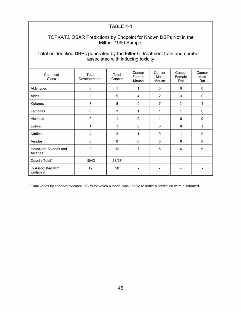
TABLE 4-4
TOPKAT® OSAR Predictions by Endpoint for Known DBPs Not in the Miltner 1990 Sample
Total unidentified DBPs generated by the Filter-Cl treatment train and number associated with inducing toxicity
Chemical Class
Total Developmental
0
3
7
0
0
1
4
0
3
18/43
% Associated with Endpoint
42 58 - ---
Aldyhydes
Acids
Ketones
Lactones
Alcohols
Esters
Nitriles
Amides
Halo/Nitro Alkanes and Alkenes
Count / Total*
Total Cancer
Cancer Female Mouse
Cancer Male
Mouse
Cancer Female
Rat
Cancer Male Rat
1 1 0 0 0
5
8 0 7 0 3
3 1 1 1 0
1 0 1 0 0
1 0
2 1 0 1 0
0 0 0 0 0
12 7 5
33/57 -
0 3 2 4
1 0 0
6 6
---
* Total varies by endpoint because DBPs for which a model was unable to make a prediction were eliminated.
45
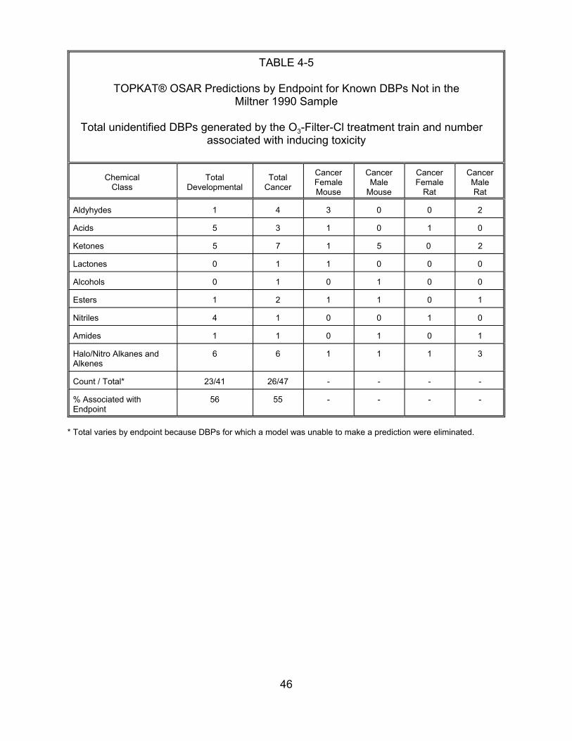
TABLE 4-5
TOPKAT® OSAR Predictions by Endpoint for Known DBPs Not in the Miltner 1990 Sample
Total unidentified DBPs generated by the O3-Filter-Cl treatment train and number associated with inducing toxicity
Chemical Class
Total Developmental
1
5
5
0
0
1
4
1
6
23/41
% Associated with Endpoint
56 55 - ---
Aldyhydes
Acids
Ketones
Lactones
Alcohols
Esters
Nitriles
Amides
Halo/Nitro Alkanes and Alkenes
Count / Total*
Total Cancer
Cancer Female Mouse
Cancer Male
Mouse
Cancer Female
Rat
Cancer Male Rat
4 3 0 0 2
3
7 1 5 0 2
1 1 0 0 0
1 0 1 0 0
2 1
1 0 0 1 0
1 0 1 0 1
6 1
26/47 -
0 1 0 1
1 0 1
3 1 1
---
* Total varies by endpoint because DBPs for which a model was unable to make a prediction were eliminated.
46
used as surrogates for the fraction of unidentified DBPs that may be associated with
inducing reproductive toxicity (" Repro).
Note that the QSAR model was unable to classify some of the chemicals with
respect to some health endpoints. These chemicals were omitted from the analysis.
Since the number of chemicals that could not be classified differed by endpoint,
thedenominators for the fraction of DBPs associated with inducing cancer (57 and 41 for
the filter-Cl and O3-filter-Cl treatments, respectively) differed from the denominators of
the corresponding fractions for developmental toxicity (43 and 47, respectively).
It is recognized that there is considerable uncertainty in these estimates due to
many factors: the assumption that the proportion of unidentified chemicals associated
with inducing a health effect is equal to the proportion of chemicals by OX concentration
in :g Cl/L associated with inducing that health endpoint; unknowns relative to the actual
number, proportions, and molecular weights of chemicals that make up the unidentified
TOX; potential risks from the unidentified material that does not fall into the
classification of organic halides; and possible classification errors by the TOPKAT®
program. This is only one method that could be used for estimating toxicity for
unidentified TOX. Increased information relative to the uncertainties listed here or use
of additional QSAR models could improve the accuracy of the estimates. Because of
these uncertainties, it is recognized that the estimated risks from exposure to the
unidentified TOX could be very broad in range and could conceivably include zero.
4.2.3. Model Uncertainty Introduced by Estimates of TOX Potency. It is recognized
that there are a number of uncertain factors affecting the estimate of the risk contributed
by unidentified DBPs
47
• The actual number of and molecular weights of the chemicals that make up the unidentified DBPs unknown.
• The proportion of unidentified DBPs associated with each endpoint has been estimated from a generic list of DBPs, rather than from lists specific to each drinking water treatment train under consideration.
• Statistical models built into the TOPKAT® software may have introduced classification errors.
• The risk posed by the unidentified DBPs assumed to be the same as it is for the identified DBPs on a :g OX/L basis. This assumption implies that DBPs with no OX component pose no risk.
Additional information addressing the sources of uncertainty listed here or use of
additional QSAR models could improve the accuracy and precision of the estimates.
Because of these uncertain factors, it is recognized that the plausible range of risks
from exposure to the unidentified DBPs is very broad and could conceivably include
zero.
4.3. INCREMENTAL RISK PER :g/L FOR THE IDENTIFIED DBPs
Carcinogenicity (Section 4.1), developmental toxicity (Section 4.2), and
reproductive toxicity (Section 4.2) were estimated using animal bioassay data.
Appendix B.4 summarizes these data. Section 4.3.3 discusses the use of
epidemiological data to estimate risks associated with DBP exposure. Section 4.3.4
discusses the implications of assuming that the DBP slope factor distributions are
statistically independent.
4.3.1. Cancer. The distribution of plausible values for each DBP’s cancer slope factor
was estimated using the linearized multi-stage model results applied to animal bioassay
data. It was assumed that the distribution of plausible values is lognormal, with a
geometric mean equal to the estimated MLE, and a 95th percentile equal to the upper
95% confidence limit on the slope. While maximum likelihood theory suggests that
48
parameter values have a normal distribution, the skewed nature of the confidence
intervals for these slope parameters (very large standard errors relative to the mean
estimate) suggests that the normality assumption does not hold in this case. Table 4-6
summarizes the slope factor estimates for those DBPs that are suspected carcinogens.
With the exception of DCA, TCA, and chloroform, the oral upper bound slope
estimates for the cancer endpoint were taken directly from EPA’s Integrated Risk
Information System (IRIS) (U.S. EPA, 2000) for bromate, chloroform (CHCl3),
bromodichloromethane (BDCM), chlorodibromomethane (CDBM), and bromoform
(CHBr3). The upper bound slope estimate for chloral hydrate (CH) is a verified IRIS
workgroup value that has not been loaded onto IRIS to date. All of these values were
computed for excess risk, using the linearized multistage model that assumes a low
dose linear response. The mean slope estimates for these chemicals were computed
by re-running the linearized multistage model on the IRIS/workgroup data sets and
taking the Maximum Likelihood Estimate (MLE) value. Because the body weight
conversions for the DBPs on IRIS were based on the assumption of 2/3 power, this
assumption was maintained for consistency. The 1996 draft Cancer Guidelines (US
EPA, 1996) have proposed the use of 3/4 power for the conversion.
As discussed in Section 4.1.3, this risk assessment assumes that for mechanistic
reasons, chloroform’s cancer dose-response relationship has a threshold well above
environmentally relevant levels. Since chloroform’s estimated concentration is below its
estimated threshold, this DBP is assumed not to contribute to carcinogenicity. (If the
assumption of linearity were imposed, the methodology used here would estimate
chloroform’s slope factor distribution to be lognormal with a geometric mean of
3.1 x 10⁻³, and a geometric standard deviation of 1.5.)
49
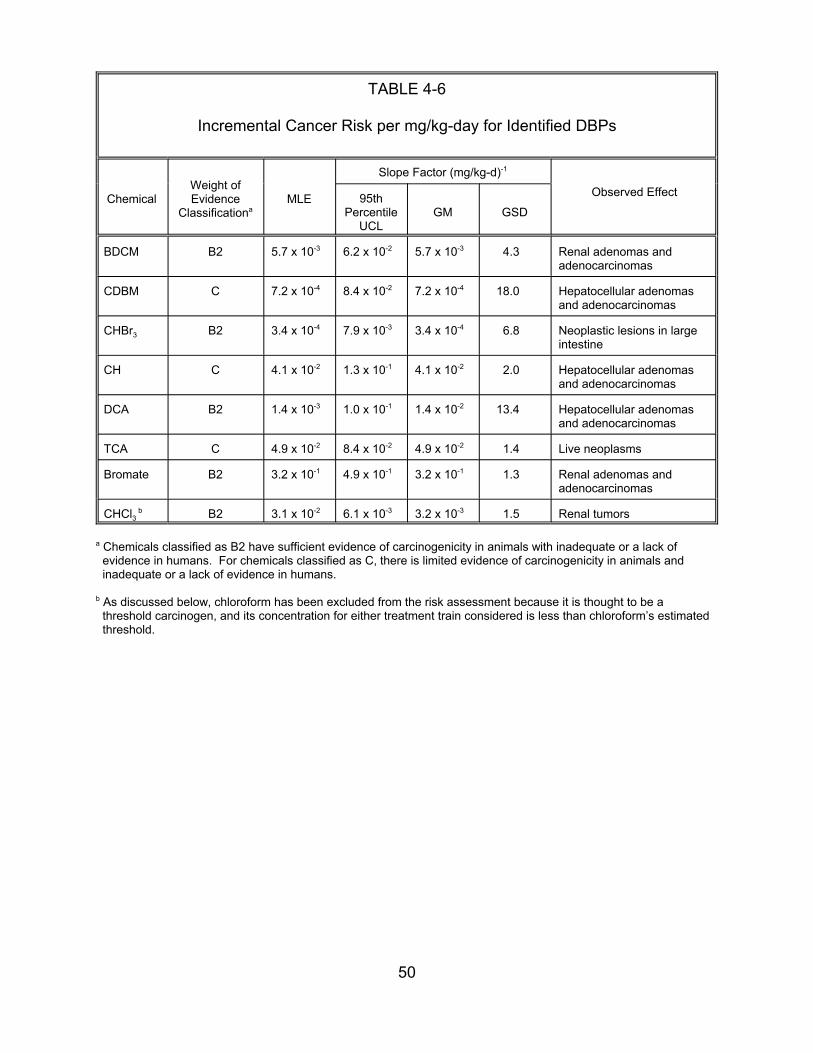
TABLE 4-6
Incremental Cancer Risk per mg/kg-day for Identified DBPs
Weight of Slope Factor (mg/kg-d)-1
Chemical Evidence Classificationa
MLE Observed Effect 95th Percentile
UCL GM GSD
BDCM B2 5.7 x 10⁻³ 6.2 x 10⁻² 5.7 x 10⁻³ 4.3 Renal adenomas and adenocarcinomas
CDBM C 7.2 x 10⁻⁴ 8.4 x 10⁻² 7.2 x 10⁻⁴ 18.0 Hepatocellular adenomas and adenocarcinomas
CHBr3 B2 3.4 x 10⁻⁴ 7.9 x 10⁻³ 3.4 x 10⁻⁴ 6.8 Neoplastic lesions in large intestine
CH C 4.1 x 10⁻² 1.3 x 10⁻¹ 4.1 x 10⁻² 2.0 Hepatocellular adenomas and adenocarcinomas
DCA B2 1.4 x 10⁻³ 1.0 x 10⁻¹ 1.4 x 10⁻² 13.4 Hepatocellular adenomas and adenocarcinomas
TCA C 4.9 x 10⁻² 8.4 x 10⁻² 4.9 x 10⁻² 1.4 Live neoplasms
Bromate B2 3.2 x 10⁻¹ 4.9 x 10⁻¹ 3.2 x 10⁻¹ 1.3 Renal adenomas and adenocarcinomas
CHCl3 b B2 3.1 x 10⁻² 6.1 x 10⁻³ 3.2 x 10⁻³ 1.5 Renal tumors
a Chemicals classified as B2 have sufficient evidence of carcinogenicity in animals with inadequate or a lack of evidence in humans. For chemicals classified as C, there is limited evidence of carcinogenicity in animals and inadequate or a lack of evidence in humans.
b As discussed below, chloroform has been excluded from the risk assessment because it is thought to be a threshold carcinogen, and its concentration for either treatment train considered is less than chloroform’s estimated threshold.
50
For dichloroacetic acid (DCA) and trichloroacetic acid (TCA), quantitative cancer
estimates are not available on IRIS, but qualitative assessments there list B2 and C
cancer classifications, respectively. The upper bound and mean (MLE) slope factors for
DCA and TCA were back-calculated from risk levels given in Bull and Kopfler (1991).
DCA was also reviewed by the same expert panel as chloroform; the panel indicated
that there is insufficient evidence that tumors occur at low doses of DCA in animal
studies (U.S. EPA, 1998b); thus it is questionable whether the mechanism of action for
cancer is active at the low levels to which humans are exposed. However, the Agency
position on DCA falls short of employing the same MOE methodology as was applied in
the case of chloroform. For this reason, and because Agency text (U.S. EPA, 1998b)
leaves open the question of low dose mechanism, DCA was kept in the case study
analysis of cancer risk.
4.3.2. Developmental and Reproductive Toxicity. As with cancer, the distribution of
plausible values for the “slope factors” for developmental and reproductive toxicity were
estimated using the linearized multi-stage model results applied to animal bioassay
data. Likewise, it was assumed that the distribution of plausible values is lognormal,
with a geometric mean equal to the estimated MLE, and a 95th percentile equal to the
upper 95% confidence limit on the slope. Tables 4-7 and 4-8 summarize these
estimates.
Several of these chemicals have Reference Doses (RfDs) listed on IRIS (U.S.
EPA, 2000), so the estimation of risks at exposures below the RfDs is of concern.
However, the RfD values are not useful in this risk assessment for several reasons.
First, RfDs are endpoint-specific sub-threshold levels that do not yield the dose-
response information needed for the case study. Second, this risk assessment
51
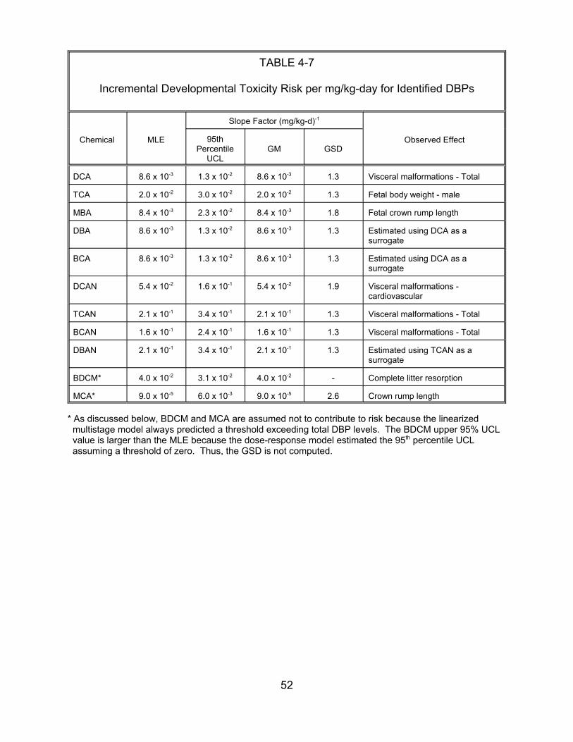
TABLE 4-7
Incremental Developmental Toxicity Risk per mg/kg-day for Identified DBPs
Chemical MLE
Slope Factor (mg/kg-d)-1
Observed Effect 95th Percentile
UCL GM GSD
DCA 8.6 x 10⁻³ 1.3 x 10⁻² 8.6 x 10⁻³ 1.3 Visceral malformations - Total
TCA 2.0 x 10⁻² 3.0 x 10⁻² 2.0 x 10⁻² 1.3 Fetal body weight - male
MBA 8.4 x 10⁻³ 2.3 x 10⁻² 8.4 x 10⁻³ 1.8 Fetal crown rump length
DBA 8.6 x 10⁻³ 1.3 x 10⁻² 8.6 x 10⁻³ 1.3 Estimated using DCA as a surrogate
BCA 8.6 x 10⁻³ 1.3 x 10⁻² 8.6 x 10⁻³ 1.3 Estimated using DCA as a surrogate
DCAN 5.4 x 10⁻² 1.6 x 10⁻¹ 5.4 x 10⁻² 1.9 Visceral malformations -cardiovascular
TCAN 2.1 x 10⁻¹ 3.4 x 10⁻¹ 2.1 x 10⁻¹ 1.3 Visceral malformations - Total
BCAN 1.6 x 10⁻¹ 2.4 x 10⁻¹ 1.6 x 10⁻¹ 1.3 Visceral malformations - Total
DBAN 2.1 x 10⁻¹ 3.4 x 10⁻¹ 2.1 x 10⁻¹ 1.3 Estimated using TCAN as a surrogate
BDCM* 4.0 x 10⁻² 3.1 x 10⁻² 4.0 x 10⁻² - Complete litter resorption
MCA* 9.0 x 10⁻⁵ 6.0 x 10⁻³ 9.0 x 10⁻⁵ 2.6 Crown rump length
* As discussed below, BDCM and MCA are assumed not to contribute to risk because the linearized multistage model always predicted a threshold exceeding total DBP levels. The BDCM upper 95% UCL value is larger than the MLE because the dose-response model estimated the 95th percentile UCL assuming a threshold of zero. Thus, the GSD is not computed.
52

TABLE 4-8
Incremental Reproductive Toxicity Risk per mg/kg-day for Identified DBPs
Chemical MLE
Slope Factor (mg/kg-d)-1
95th Percentile
UCL GM GSD
DBA
DCA
BCA
2.5 x 10⁻² 6.0 x 10⁻² 2.5 x 10⁻²
2.5 x 10⁻² 6.0 x 10⁻² 2.5 x 10⁻²
2.5 x 10⁻² 6.0 x 10⁻² 2.5 x 10⁻²
Observed Effect
1.7 Number of cauda sperm
1.7 Estimated using DBA as a surrogate
1.7 Estimated using DBA as a surrogate
assumes additivity is operational, that is, that the chemicals are acting in a joint fashion,
a fact that the RfDs themselves do not take into account. Third, the DBPs in Tables 4-7
and 4-8 may actually be the chemicals of concern, or they may be only surrogates for
other chemicals responsible for effects observed in epidemiologic studies. Finally, for
these endpoints, it is possible that a mixtures toxicity threshold exists that would
potentially be lower than any of the individual component thresholds, such that
estimation of mixtures risk at these individual subthreshold dose levels is reasonable.
Using a dose-response approach, rather than depending on RfDs, works well for this
risk assessment because of the need to compare DBP-induced risks for the endpoints
of concern at extremely low environmental exposures.
Table 4-9 summarizes the availability of developmental and reproductive dose-
response data for six of the haloacetic acids (MCA, DCA, TCA, MBA, DBA and BCA),
four of the haloacetonitriles (DCAN, TCAN, BCAN and DBAN) and one of the
trihalomethanes (BDCM).
53

TABLE 4-9
Availability of Developmental and Reproductive Dose-Response Data
Haloacetic Acids MCA DCA TCA MBA DBA BCA
Developmental Toxicitya
y, (+) y, + y, + y, +
Reproductive Toxicitya
y, +
y, -y, +
Haloacetonitriles DCAN TCAN BCAN DBAN
y, + y, + y, +
y, (-)b y, (-)b
Trihalomethanes BDCM y, +
a Data are from gavage studies in rats unless otherwise noted.
b Data are from a screening-level drinking water study in rats.
Key: y yes, adequate data available + results were positive for adverse effect- results were negative for adverse effect(+) results were marginally positive(-) results were negative, but a toxicity-based MTD could not be achieved
due to taste aversion and consequent refusal to drink higher concentrations of the chemical, and this was a short-term screening study
54
Seven of these DBPs (MCA, DCA, TCA, MCA, DCAN, TCAN, BCAN) have been
subjects of developmental toxicity studies by a single group of investigators, and three
(DCA, MBA, DBA) have been the subjects of male reproductive studies by another
group of investigators. These studies were all conducted in rats using gavage
administration. The results for developmental toxicity were positive. For reproductive
toxicity, the dihalogenated haloacetic acids produced positive results, but the
monohalogenated acetic acid (MBA) produced negative results. DBAN was tested in a
short-term developmental and reproductive toxicity screening study in rats by the NTP
(1992), with negative results. BDCM was tested in a developmental toxicity screening
bioassay with positive results. Developmental toxicity data are inadequate for DBA,
BCA, and for DBAN. A surrogate approach seemed appropriate to address these data
gaps because the available data indicated that developmental toxicity may be common
to the haloacetic acid and haloacetonitrile DBPs. As a provisional measure, DCA was
selected as a surrogate for the haloacetic acids and TCAN was selected as a surrogate
for the haloacetonitriles.
Dose-response modeling was performed on all possible developmental and
reproductive endpoints using human equivalent doses in a linearized multi-stage model
with a threshold parameter estimated by the modeling procedure. Note that some of the
data are quantal, but other data (body weight, crown-rump length) are continuous and
were converted to a quantal measure prior to modeling. Modeling results for all data
sets are found in Table 4-10. For many of the data sets, the threshold estimates were
above concentration levels for the treatment trains and were therefore not included in
any of the risk estimates. This criteria excluded MCA and BDCM entirely from the risk
calculations. For the other DBPs, the modeling procedure failed to
55

TABLE 4-10
Non-Cancer Dose-Response Modeling Results Using BW2/3 Scaling Factor
Data Set [note all are for rats except when noted
(DCA, Cicmanec et al.)]
Equiv Human
ED01 (mg/kg-d)
Equiv Human
ED10 (mg/kg-d)
Threshold (mg/kg-d)
MCA Smith et al., Fetal body weight MCA MCA Smith et al., Visceral Malformations
Smith et al., Crown-rump length
DCA Smith et al., Fetal body weight -male DCA female DCA male DCA female DCA malformations Total DCA malformations Cardiovascular
Smith et al., Fetal body weight -
Smith et al., Crown-rump length -
Smith et al., Crown-rump length -
Smith et al., Visceral
Smith et al., Visceral
TCA Smith et al., Complete litter resorption TCA loss/litter TCA male TCA female TCA length - male TCA length - female TCA malformations Total TCA malformations Cardiovascular, total TCA malformations Levacardia
Smith et al., % Postimplantation
Smith et al., Fetal body weight -
Smith et al., Fetal body weight -
Smith et al., Fetal crown-rump
Smith et al., Fetal crown-rump
Smith et al., Visceral
Smith et al., Visceral
Smith et al., Visceral
18.9 26.7 11.2 15.7 20.2 11.2 16.5 21.8 11.2
4.7 27.3 2.2
18.6 40.4 16.3
5.1 36.2 1.0
5.1 36.2 1.0
1.2 12.2 0
1.7 17.6 0
110.5 143.2 106.3
51.1 88.9 46.8
0.5 5.2 0
0.6 6.0 0
16.2 26.8 15.0
22.9 37.9 21.4
25.7 32.2 25.0
11.9 23.4 10.7
1.3 13.8 0
56
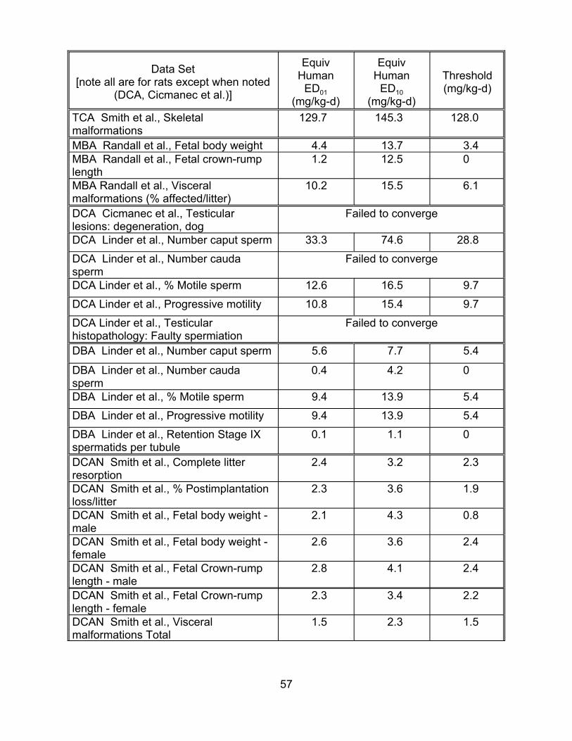
Data Set [note all are for rats except when noted
(DCA, Cicmanec et al.)]
TCA malformations
Smith et al., Skeletal
MBA Randall et al., Fetal body weight MBA Randall et al., Fetal crown-rump length MBA Randall et al., Visceral malformations (% affected/litter) DCA Cicmanec et al., Testicular lesions: degeneration, dog DCA
DCA sperm DCA Linder et al., % Motile sperm
DCA Linder et al., Progressive motility
DCA Linder et al., Testicular histopathology: Faulty spermiation
Linder et al., Number caput sperm
Linder et al., Number cauda
DBA Linder et al., Number caput sperm
DBA sperm DBA
DBA
DBA spermatids per tubule
Linder et al., Number cauda
Linder et al., % Motile sperm
Linder et al., Progressive motility
Linder et al., Retention Stage IX
DCAN Smith et al., Complete litter resorption DCAN loss/litter DCAN male DCAN female DCAN length - male DCAN length - female DCAN malformations Total
Smith et al., % Postimplantation
Smith et al., Fetal body weight -
Smith et al., Fetal body weight -
Smith et al., Fetal Crown-rump
Smith et al., Fetal Crown-rump
Smith et al., Visceral
Equiv Human
ED01 (mg/kg-d)
Equiv Human
ED10 (mg/kg-d)
Threshold (mg/kg-d)
129.7 145.3 128.0
4.4 13.7 3.4 1.2 12.5 0
10.2 15.5 6.1
Failed to converge
33.3 74.6 28.8
Failed to converge
12.6 16.5 9.7
10.8 15.4 9.7
Failed to converge
5.6 7.7 5.4
0.4 4.2 0
9.4 13.9 5.4
9.4 13.9 5.4
0.1 1.1 0
2.4 3.2 2.3
2.3 3.6 1.9
2.1 4.3 0.8
2.6 3.6 2.4
2.8 4.1 2.4
2.3 3.4 2.2
1.5 2.3 1.5
57
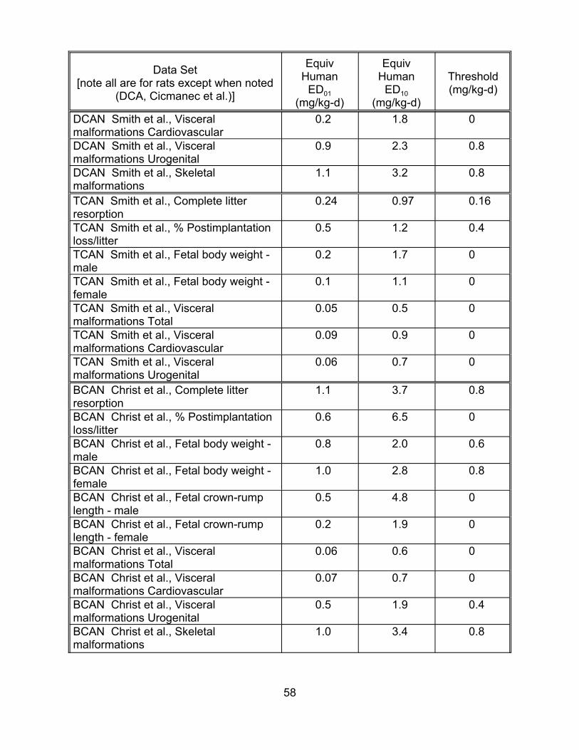
Data Set [note all are for rats except when noted
(DCA, Cicmanec et al.)]
DCAN malformations Cardiovascular DCAN malformations Urogenital DCAN malformations
Smith et al., Visceral
Smith et al., Visceral
Smith et al., Skeletal
TCAN Smith et al., Complete litter resorption TCAN loss/litter TCAN male TCAN female TCAN malformations Total TCAN malformations Cardiovascular TCAN malformations Urogenital
Smith et al., % Postimplantation
Smith et al., Fetal body weight -
Smith et al., Fetal body weight -
Smith et al., Visceral
Smith et al., Visceral
Smith et al., Visceral
BCAN Christ et al., Complete litter resorption BCAN loss/litter BCAN male BCAN female BCAN length - male BCAN length - female BCAN malformations Total BCAN malformations Cardiovascular BCAN malformations Urogenital BCAN malformations
Christ et al., % Postimplantation
Christ et al., Fetal body weight -
Christ et al., Fetal body weight -
Christ et al., Fetal crown-rump
Christ et al., Fetal crown-rump
Christ et al., Visceral
Christ et al., Visceral
Christ et al., Visceral
Christ et al., Skeletal
Equiv Human
ED01 (mg/kg-d)
Equiv Human
ED10 (mg/kg-d)
Threshold (mg/kg-d)
0.2 1.8 0
0.9 2.3 0.8
1.1 3.2 0.8
0.24 0.97 0.16
0.5 1.2 0.4
0.2 1.7 0
0.1 1.1 0
0.05 0.5 0
0.09 0.9 0
0.06 0.7 0
1.1 3.7 0.8
0.6 6.5 0
0.8 2.0 0.6
1.0 2.8 0.8
0.5 4.8 0
0.2 1.9 0
0.06 0.6 0
0.07 0.7 0
0.5 1.9 0.4
1.0 3.4 0.8
58
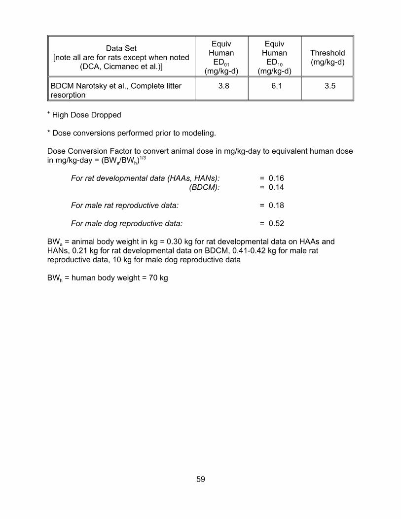
Data Set [note all are for rats except when noted
(DCA, Cicmanec et al.)]
Equiv Human
ED01 (mg/kg-d)
EquivHuman
ED10 (mg/kg-d)
Threshold (mg/kg-d)
BDCM Narotsky et al., Complete litter resorption
3.8 6.1 3.5
+ High Dose Dropped
* Dose conversions performed prior to modeling.
Dose Conversion Factor to convert animal dose in mg/kg-day to equivalent human dose in mg/kg-day = (BWa/BWh)1/3
For rat developmental data (HAAs, HANs): = 0.16 (BDCM): = 0.14
For male rat reproductive data: = 0.18
For male dog reproductive data: = 0.52
BWa = animal body weight in kg = 0.30 kg for rat developmental data on HAAs and HANs, 0.21 kg for rat developmental data on BDCM, 0.41-0.42 kg for male rat reproductive data, 10 kg for male dog reproductive data
BWh = human body weight = 70 kg
59
estimate a threshold value for one or more of the data sets such that the threshold was
effectively set to zero. For these cases, scientific judgment was used to look across
these data sets for the strongest data set and model results, using factors such as
evidence of dose-response in the raw data, larger sample sizes, and adequate
goodness-of-fit of the model, to choose a dose-response model. For the calculations of
extra risk that were made from these data sets, the estimates made directly from the
model were identical to those calculated from the slope factors alone because the low
dose region of the dose-response curve is relevant in this context. Therefore, MLE and
upper bound slope factors were taken from the modeling results for use in risk
estimation.
For MCA and BDCM, all the data sets produced thresholds exceeding likely total
environmental DBP levels (thresholds of 11.2 mg/kg-day and 3.5 mg/kg-day,
respectively). These chemicals therefore contributed nothing to the non-carcinogen risk
estimates. For the other DBPs, the modeling procedure failed to estimate a positive
threshold value for one or more of the data sets. For these data sets, the threshold was
assumed to be zero. In these cases, scientific judgment was used to identify the
strongest single data set to quantify risk, using factors such as evidence of dose-
response in the raw data, sample size, and model goodness-of-fit. For the calculations
of extra risk that were made from these data sets, the estimates made directly from the
model were identical to those calculated from the slope factors alone because the low
dose region of the dose-response curve is relevant in this context. Therefore, MLE and
upper bound slope factors from the modeling results were used for risk estimation.
Note that in place of the approach used here of estimating risk from the single
best data set for which there was no positive threshold, the risk assessment could have
60
alternatively summed the risks (i.e., the slopes) calculated for all such data sets for each
DBP. It may be appropriate to sum the risks from multiple data sets if these data sets
truly represent distinct types of developmental or reproductive toxicity. For example, in
the case of developmental toxicity, if the unit risk for a DBP is 5 x 10⁻⁴ for visceral
malformations and 3 x 10⁻⁴ for fetal crown-rump length, it may be appropriate to
conclude that, in the absence of other data, the collective unit risk for either visceral
malformations or an abnormal fetal crown-rump length is 8 x 10⁻⁴. On the other hand, if
in the case of reproductive toxicity, there is a unit risk estimate based on testicular
histopathology and another risk estimate for abnormal caput sperm count, it may be
inappropriate to sum risks if it is believed the abnormal caput sperm count is a
manifestation of cellular abnormalities that were assessed in the histopathology data
set.
It should also be noted that while some of the data listed in Table 4-10 are
quantal, other data (body weight, crown-rump length) are continuous. The continuous
data were converted to quantal data (estimated # of litters affected in the table) prior to
modeling. Conversion of the continuous-response developmental data to quantal form
was performed by assuming a normal distribution with a constant variance across dose
groups for the response, and a 5% background response rate. Because individual
animal data were not available, the number of responders in each dose group was
estimated by first establishing a critical value representing the point above which (or
below which, depending on the direction of adverse response) 5% of the control group
lies. Then for each dose group the proportion exceeding this critical value was
estimated. This proportion was applied to the number of animals in the dose group to
determine the number of responders. The doses were converted to equivalent human
61
doses using the scaling factor of body weight to the 2/3 power, an approach that is
consistent with the conversions used for the Agency verified cancer slope factors used
in this risk assessment.
4.3.3. Use of Epidemiological Data to Estimate Risk. This section summarizes
epidemiological data that could be used in place of or in conjunction with the animal
bioassay data to quantify DBP carcinogenicity. This literature is further described in
Appendix C. While this literature is not used in the risk assessment’s base analysis, it
will be used in Section 5 to investigate the potential importance of model and data
uncertainty introduced by reliance on animal bioassay data to estimate toxicity. For
reasons discussed in Appendix C, the epidemiological literature will not be used to
produce alternative estimates of developmental and reproductive toxicity. However, the
epidemiological literature investigating the putative association between drinking water
disinfection and cancer will be used to calculate an alternative incremental cancer risk
per :g/L total OX (in :g Cl/L).
Use of this information to estimate risks associated with the treatment trains
investigated here is complicated by the following factors:
• The studies do not provide quantitative measures of exposure to specific DBPs;
• The studies are not directly applicable to the treatment trains investigated here;
• The results are expressed in terms of relative risk, rather than the incremental probability of some outcome per unit intake; and
• The results are affected by general design problems affecting observational epidemiological studies (e.g., confounding, loss to follow-up, etc.).
62

Appendix C.2 is a review performed by NCEA Cincinnati of the epidemiological
literature investigating the putative association between drinking water disinfection and
cancer. Although investigators have reported an association between exposure to
chlorinated drinking water and several types of cancer, the review concludes that a lack
of findings or inconsistencies in these results preclude the derivation of a reasonable
odds ratio (OR) estimate in all cases except bladder cancer. In that case, NCEA finds
that the OR may be as high as 1.5, although it is very likely to be lower, and perhaps
even 1.0, indicating no excess risk.
4.3.4. The Assumption of Statistical Independence. As noted in the introduction to
Section 4, the baseline risk assessment assumes that the slope factor distributions for
each of the DBPs are statistically independent. That is, new information, for example,
that the true slope factor for DBP1 is much higher than its original central estimate does
not make it more likely that the slope factor for DBP2 is also much higher than its
original central estimate. It is conceivable that, for each health endpoint, the slope
factors are positively correlated if the same type of error affects all of the animal
bioassays in the same way. For example, the animals used in the bioassays may be
more sensitive to DBP carcinogenicity than humans. In this case, all the DBP
carcinogenicity estimates may be too high. Section 5 investigates the potential impact
of incorrectly assuming statistical independence among the slope factor estimates.
63
5. RESULTS
5.1. ESTIMATED RISK
Figures 5-1 through 5-9 illustrate the cancer risks (5-1 through 5-3),
developmental toxicity risks (5-4 through 5-6), and reproductive toxicity risks (5-7
through 5-9) associated with the two drinking water treatment trains considered here;
they also illustrate the difference in risk between the two treatment trains:
• The first of the three figures for each health endpoint illustrates risks associated with the filter-Cl treatment train.
• The second illustrates risks associated with the O3-filter-Cl treatment train.
• The third illustrates the risk reduction achieved by supplementing filter-Cl with ozone pretreatment. Negative values represent cases in which ozone pretreatment increases risk (i.e., the “improvement” is negative).
The horizontal axis in each figure represents variability (population heterogeneity
introduced by differences in tap water consumption), and the vertical axis in each figure
represents uncertainty. For example, the cancer risk incurred by the median individual
exposed to water treated by the filter-Cl treatment train (Figure 5-1) is represented by
the box and whiskers plot lying above the 50th percentile point on the horizontal axis.
The box and whiskers plot above that point on the horizontal axis illustrates the
following for the median individual:
The median risk, indicated by the horizontal line inside the rectangle;
• The interquartile confidence interval for risk (i.e., the 25th and 75th percentile for risk), indicated by the top and the bottom of the rectangle;
• The “upper confidence limit” and “lower confidence limit,”3 indicated by the whiskers extending from the rectangle;
3 The box and whisker plot was created using Systat version 8.0 (SPSS, 1998, Graphics Volume, p. 94). The documentation states that the lower whisker extends to a value that equals the 1st quartile minus 1.5 times the difference between the median and the lower quartile. The upper whisker extends to a value that equals the 3rd quartile plus 1.5 times the difference between the upper quartile and the median.
64
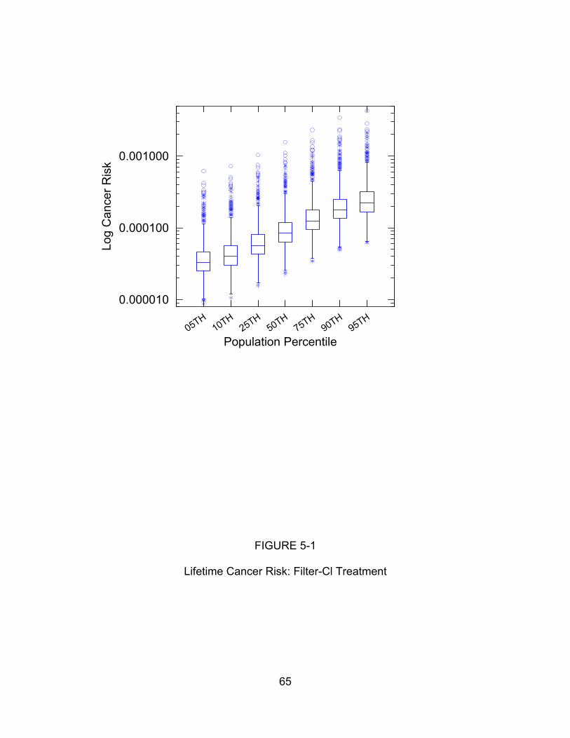
0.001000
Log
Can
cer R
isk
0.000100
0.000010
H1
H2
H5
H7
H9
H9
H50 T T0 T5 T0 T5 T0 T5
Population Percentile
FIGURE 5-1
Lifetime Cancer Risk: Filter-Cl Treatment
65
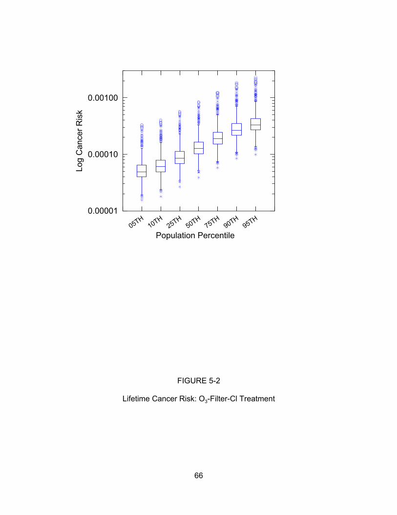
0.00100
Log
Can
c er R
isk
0.00010
0.00001H
1H
2H
5H
7H
9H
9H
50 T T0 T5 T0 T5 T0 T5
Population Percentile
FIGURE 5-2
Lifetime Cancer Risk: O3-Filter-Cl Treatment
66
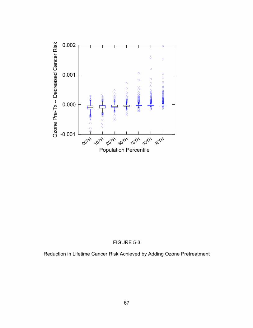
0.002
Ozo
n e P
re-T
x --
Dec
rea s
ed C
ance
r Ris
k
0.001
0.000
-0.001 H
1H
2H
5H
7H
9H
9H
50 T T0 T5 T0 T5 T0 T5
Population Percentile
FIGURE 5-3
Reduction in Lifetime Cancer Risk Achieved by Adding Ozone Pretreatment
67
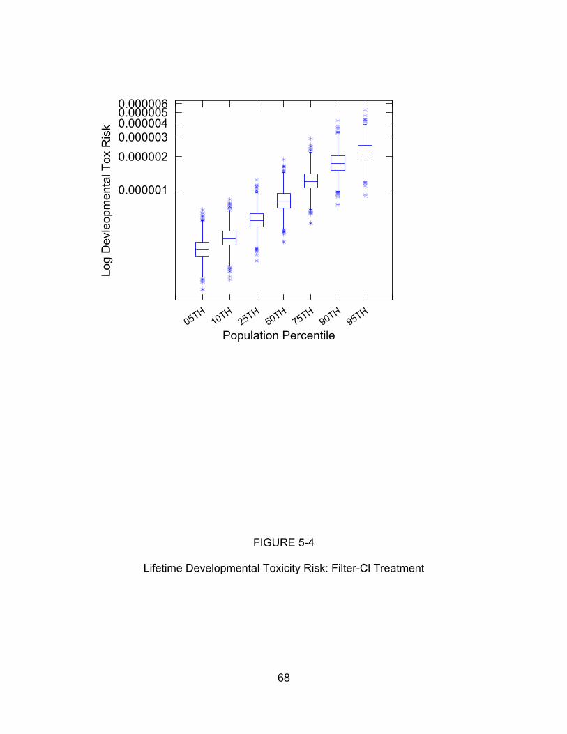
0.0000060.0000050.000004
Log
Dev
leop
men
t al T
ox R
isk
0.000003
0.000002
0.000001
50 TH1
H2
TH55
H7
TH95
H9
TH5T0 T0 T0
Population Percentile
FIGURE 5-4
Lifetime Developmental Toxicity Risk: Filter-Cl Treatment
68
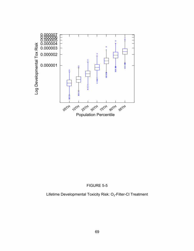
0.0000070.0000060.0000050.0000040.000003
0.000002
0.000001
Log
Dev
elop
men
t al T
ox R
isk
50 TH1
H2
TH55
H7
TH95
H9
TH5T0 T0 T0
Population Percentile
FIGURE 5-5
Lifetime Developmental Toxicity Risk: O3-Filter-Cl Treatment
69
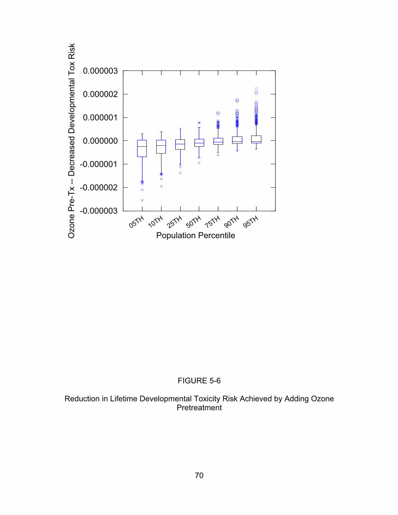
0.000003O
zon e
Pre
-Tx
--D
ecre
a sed
Dev
elo p
men
tal T
ox R
isk
0.000002
0.000001
0.000000
-0.000001
-0.000002
-0.000003 H
1H
2H
5H
7H
9H
9H
50 T T0 T5 T0 T5 T0 T5
Population Percentile
FIGURE 5-6
Reduction in Lifetime Developmental Toxicity Risk Achieved by Adding Ozone Pretreatment
70

Log
Rep
rodu
c tiv
e T o
x R
isk
0.0000100
0.0000010
0.0000001H
1H
2H
5H
7H
9H
9H
50 T T0 T5 T0 T5 T0 T5
Population Percentile
FIGURE 5-7
Lifetime Reproductive Toxicity Risk: Filter-Cl Treatment
71
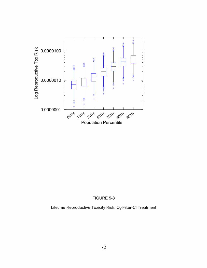
Log
Rep
rodu
c tiv
e T o
x R
isk
0.0000100
0.0000010
0.0000001
50 TH1
H2
TH55
H7
TH95
H9
TH5T0 T0 T0
Population Percentile
FIGURE 5-8
Lifetime Reproductive Toxicity Risk: O3-Filter-Cl Treatment
72
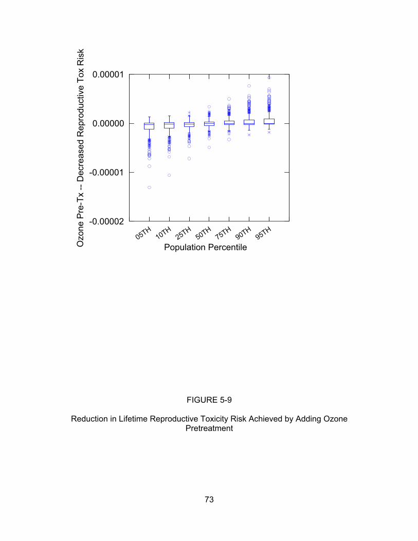
0.00001O
z one
Pr e
-Tx
- -D
ecr e
ased
Rep
r odu
cti v
e To
x R
isk
0.00000
-0.00001
-0.00002 50 TH
1H
2TH
55H
7TH
95H
9TH
5T0 T0 T0
Population Percentile
FIGURE 5-9
Reduction in Lifetime Reproductive Toxicity Risk Achieved by Adding Ozone Pretreatment
73

• Additional simulation results extending beyond the confidence limits, indicated by individually plotted points.
Note that in the first two figures in each set of three (Figures 5-1, 5-2, 5-4, 5-5,
5-7, and 5-8), the values on the vertical axis have been log-transformed (log base 10)
because these values span several orders of magnitude in some cases. Because the
risk “improvement” plotted in the third figure in each pair (Figures 5-3, 5-6, and 5-9) is
negative in some cases, it was not possible to log-transform these results.
Finally, Table 5-1 quantifies uncertainty for the population average risk.
The population average statistics serve as a useful benchmark for the purpose of
assessing the relative importance of parametric uncertainty (reflected in Table 5-1) and
other sources of uncertainty (reviewed in Section 5.3).
5.2. PARAMETRIC UNCERTAINTY
Tables 5-2, 5-3, and 5-4 list for cancer, developmental toxicity, and reproductive
toxicity, the fraction of the variance explained by each of the uncertain quantities
considered in the risk assessment. Note that for each health endpoint, the tables
include only those DBPs thought to contribute to toxicity.
5.3. NON-PARAMETRIC UNCERTAINTY
This section reviews the sources of uncertainty identified in Sections 3 and 4 that
could not be quantitatively parameterized and hence are not addressed in Section 5.2.
5.3.1. Exposure Assumptions.
5.3.1a. Tap Water Intake: The Assumption that the Ingestion Pathway Dominates
Intake. While there are no comprehensive and readily available data on the quantity of
water that taken into the body via pathways other than ingestion, it is difficult to imagine
that these alternative pathways more than double total intake. However, exposure via
74
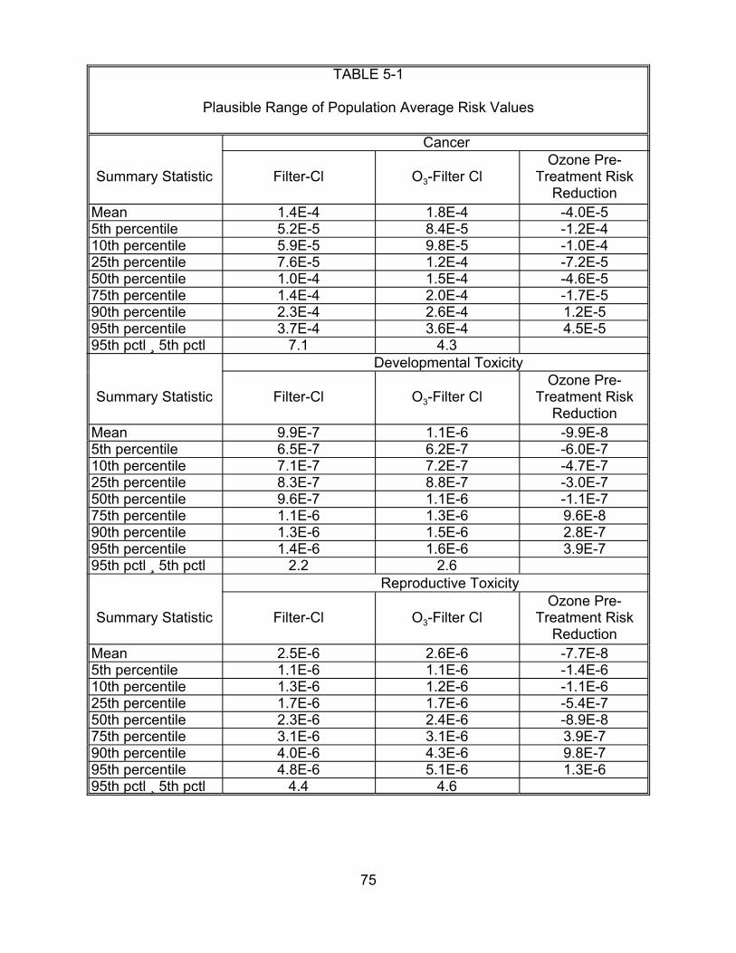
TABLE 5-1
Plausible Range of Population Average Risk Values
Cancer
Summary Statistic Filter-Cl O3-Filter Cl Ozone Pre-
Treatment Risk Reduction
Mean 1.4E-4 1.8E-4 -4.0E-5 5th percentile 5.2E-5 8.4E-5 -1.2E-4 10th percentile 5.9E-5 9.8E-5 -1.0E-4 25th percentile 7.6E-5 1.2E-4 -7.2E-5 50th percentile 1.0E-4 1.5E-4 -4.6E-5 75th percentile 1.4E-4 2.0E-4 -1.7E-5 90th percentile 2.3E-4 2.6E-4 1.2E-5 95th percentile 3.7E-4 3.6E-4 4.5E-5 95th pctl ¸ 5th pctl 7.1 4.3
Developmental Toxicity
Summary Statistic Filter-Cl O3-Filter Cl Ozone Pre-
Treatment Risk Reduction
Mean 9.9E-7 1.1E-6 -9.9E-8 5th percentile 6.5E-7 6.2E-7 -6.0E-7 10th percentile 7.1E-7 7.2E-7 -4.7E-7 25th percentile 8.3E-7 8.8E-7 -3.0E-7 50th percentile 9.6E-7 1.1E-6 -1.1E-7 75th percentile 1.1E-6 1.3E-6 9.6E-8 90th percentile 1.3E-6 1.5E-6 2.8E-7 95th percentile 1.4E-6 1.6E-6 3.9E-7 95th pctl ¸ 5th pctl 2.2 2.6
Reproductive Toxicity
Summary Statistic Filter-Cl O3-Filter Cl Ozone Pre-
Treatment Risk Reduction
Mean 2.5E-6 2.6E-6 -7.7E-8 5th percentile 1.1E-6 1.1E-6 -1.4E-6 10th percentile 1.3E-6 1.2E-6 -1.1E-6 25th percentile 1.7E-6 1.7E-6 -5.4E-7 50th percentile 2.3E-6 2.4E-6 -8.9E-8 75th percentile 3.1E-6 3.1E-6 3.9E-7 90th percentile 4.0E-6 4.3E-6 9.8E-7 95th percentile 4.8E-6 5.1E-6 1.3E-6 95th pctl ¸ 5th pctl 4.4 4.6
75
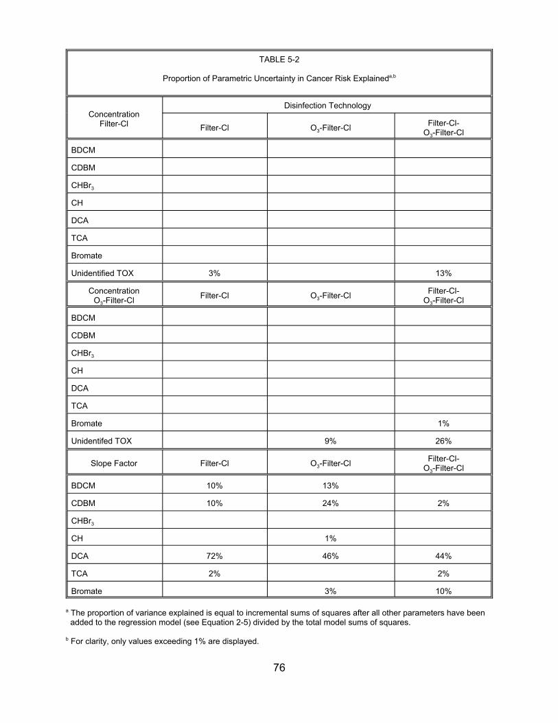
TABLE 5-2
Proportion of Parametric Uncertainty in Cancer Risk Explaineda,b
Concentration Filter-Cl
Disinfection Technology
Filter-Cl O3-Filter-Cl Filter-Cl-O3-Filter-Cl
BDCM
CDBM
CHBr3
CH
DCA
TCA
Bromate
Unidentified TOX 3% 13%
Concentration O3-Filter-Cl Filter-Cl O3-Filter-Cl Filter-Cl-
O3-Filter-Cl
BDCM
CDBM
CHBr3
CH
DCA
TCA
Bromate 1%
Unidentifed TOX 9% 26%
Slope Factor Filter-Cl O3-Filter-Cl Filter-Cl-O3-Filter-Cl
BDCM 10% 13%
CDBM 10% 24% 2%
CHBr3
CH 1%
DCA 72% 46% 44%
TCA 2% 2%
Bromate 3% 10%
a The proportion of variance explained is equal to incremental sums of squares after all other parameters have been added to the regression model (see Equation 2-5) divided by the total model sums of squares.
b For clarity, only values exceeding 1% are displayed.
76
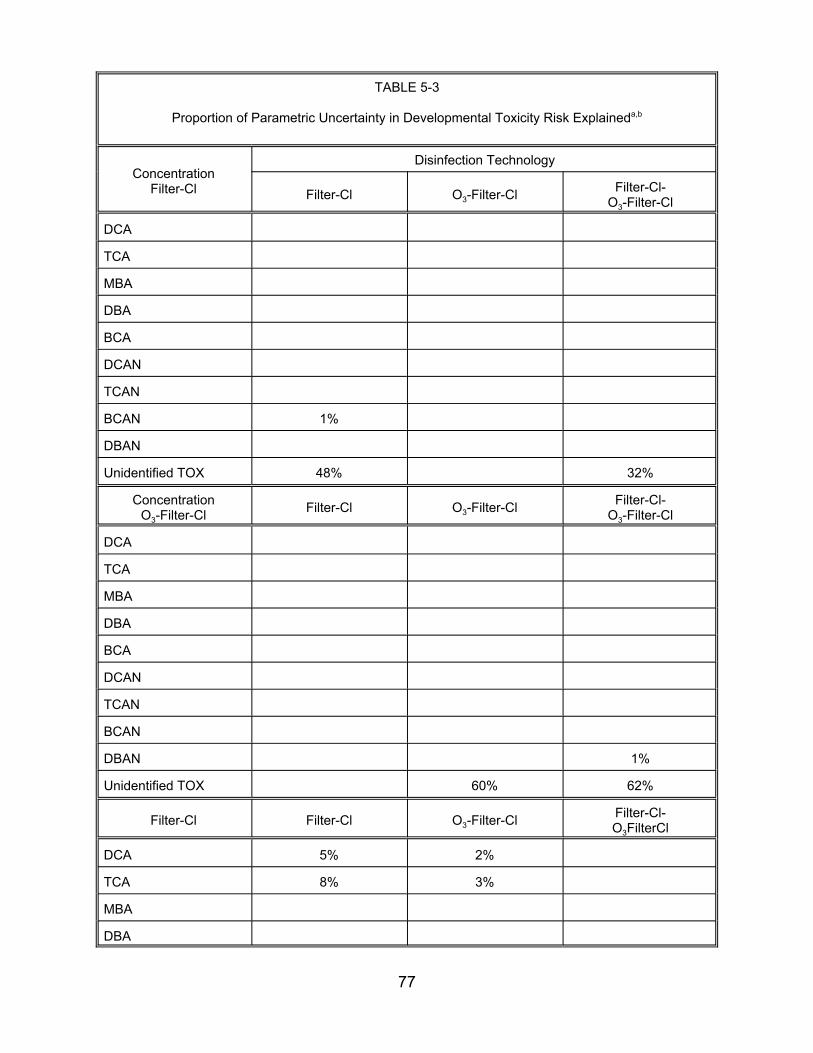
TABLE 5-3
Proportion of Parametric Uncertainty in Developmental Toxicity Risk Explaineda,b
Concentration Filter-Cl
Disinfection Technology
Filter-Cl O3-Filter-Cl Filter-Cl-O3-Filter-Cl
TCA
MBA
DBA
BCA
DCAN
TCAN
BCAN 1%
DBAN
Unidentified TOX 48%
DCA
DCA
O3-Filter-Cl
60%
O3-Filter-Cl
32%
Filter-Cl-O3-Filter-Cl
1%
62%
Filter-Cl-O3FilterCl
Concentration O3-Filter-Cl Filter-Cl
TCA
MBA
DBA
BCA
DCAN
TCAN
BCAN
DBAN
Unidentified TOX
Filter-Cl Filter-Cl
DCA 5% 2%
TCA 8% 3%
MBA
DBA
77
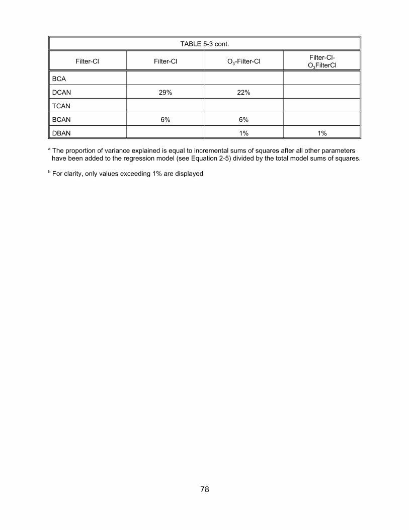
TABLE 5-3 cont.
Filter-Cl Filter-Cl O3-Filter-Cl Filter-Cl-O3FilterCl
BCA
DCAN 29% 22%
TCAN
BCAN 6% 6%
DBAN 1% 1%
a The proportion of variance explained is equal to incremental sums of squares after all other parameters have been added to the regression model (see Equation 2-5) divided by the total model sums of squares.
b For clarity, only values exceeding 1% are displayed
78
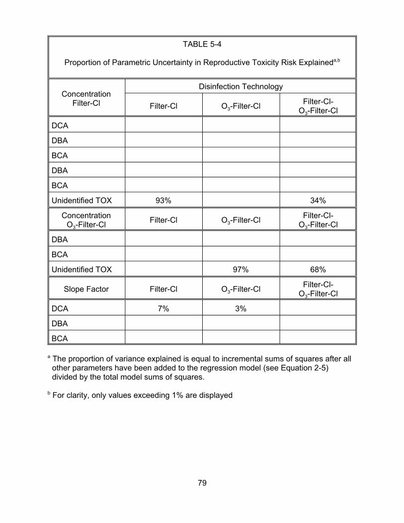
TABLE 5-4
Proportion of Parametric Uncertainty in Reproductive Toxicity Risk Explaineda,b
Concentration Filter-Cl
Disinfection Technology
Filter-Cl O3-Filter-Cl Filter-Cl-O3-Filter-Cl
DCA
DBA
BCA
DBA
BCA
Unidentified TOX
Concentration O3-Filter-Cl
DBA
BCA
Unidentified TOX
Slope Factor
DCA
DBA
BCA
93%
O3-Filter-Cl
97%
O3-Filter-Cl
3%
34%
Filter-Cl Filter-Cl-O3-Filter-Cl
68%
Filter-Cl Filter-Cl-O3-Filter-Cl
7%
a The proportion of variance explained is equal to incremental sums of squares after all other parameters have been added to the regression model (see Equation 2-5) divided by the total model sums of squares.
b For clarity, only values exceeding 1% are displayed
79
alternative pathways may pose a different unit-risk. The extent to which this may be the
case depends on factors such as the efficiency of DBP absorption via ingestion.
5.3.1b. Total Tap Water Ingestion is the Relevant Measure of Intake. As noted in
Section 3.2.3, heating tap water may remove some of the volatile DBPs. Therefore,
using total tap water as a measure of tap water intake may somewhat overstate
exposure for some DBP compounds. The Canada Department of Health and Welfare
(1981) reports both total tap water consumption and unheated tap water consumption
for individuals of various ages.4 These figures appear in Table 5-5.
Even if heating eliminated all DBPs, the data from the Canada Department of
Health indicate that the impact on exposure would not be substantial, ranging from a
decrease of 22% among children between the ages of 6 and 17, to a decrease of 62%
among some adult age groups. These results translate into a difference of a factor of
1.3 (1 ÷ 78%) to 2.5 (1 ÷ 38%). Since not all DBPs are removed by heating, the actual
impact of heating is probably less.
5.3.2. Toxicity Assumptions.
5.3.2.1. The Use of QSAR to Quantify the Fraction of Unidentified DBPs
Associated with Each Health Endpoint — The true fraction of unidentified DBPs
associated with inducing any of the three health endpoints analyzed here may range
from 0% to 100%. Table 5-6 summarizes the impact of these extreme alternative
assumptions on the mean population average risk.
4 Beverages included as unheated were drinking water, ice/mix, other types of mixes, and reconstituted milk. Categories excluded were tea, coffee, soup, homemade beer and wine, popcycles, and baby formula.
80
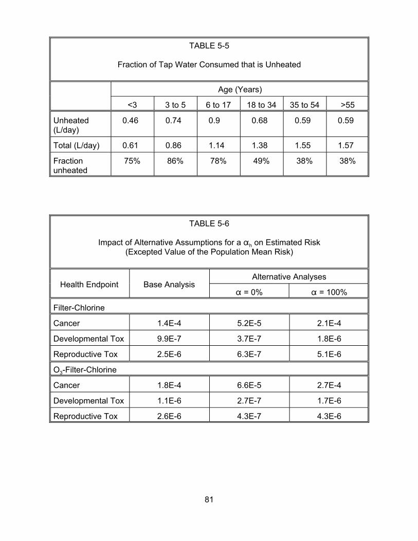
TABLE 5-5
Fraction of Tap Water Consumed that is Unheated
Age (Years)
<3 3 to 5 6 to 17 18 to 34 35 to 54 >55
Unheated 0.46 0.74 0.9 0.68 0.59 0.59(L/day)
Total (L/day) 0.61 0.86 1.14 1.38 1.55 1.57
Fraction unheated
75% 86% 78% 49% 38% 38%
TABLE 5-6
Impact of Alternative Assumptions for a " h on Estimated Risk (Excepted Value of the Population Mean Risk)
Health Endpoint Base Analysis Alternative Analyses
" = 0% " = 100%
Filter-Chlorine
Cancer
Developmental Tox
Reproductive Tox
O3-Filter-Chlorine
Cancer
Developmental Tox
Reproductive Tox
1.4E-4
1.8E-4
5.2E-5 2.1E-4
6.6E-5 2.7E-4
9.9E-7 3.7E-7 1.8E-6
2.5E-6 6.3E-7 5.1E-6
1.1E-6 2.7E-7 1.7E-6
2.6E-6 4.3E-7 4.3E-6
81
5.3.2.2. The Assumption that Unidentified DBPs Pose the Same Risk as
Identified DBPs on a µg OX/L Basis — In place of the assumption that the unidentified
DBPs pose the same risk as the identified DBPs on a mg OX/L basis (in :g Cl/L), the
analysis could alternatively assume that the unidentified DBPs pose a lesser or greater
risk. Table 5-7 summarizes the results of assuming that the risk from the unidentified
DBPs is only 50% as great as it is for the identified DBPs on a mg Cl/L basis, or that the
unidentified DBPs pose twice the risk on a mg Cl/L basis.
5.3.2.3. The Assumption that Chloroform is a Threshold Carcinogen — To
assess the impact of the assumption that chloroform is a threshold carcinogen, an
additional simulation was conducted using the assumption that the cancer dose-
response function for this DBP has no threshold. The results appear in Table 5-8.
Whether or not chloroform is a carcinogen affects the cancer risk estimate for two
reasons. First, because the concentration of chloroform substantially exceeds that of
many of the other DBPs (see Section 3.1), its potential contribution to carcinogenicity is
substantial. Second, because chloroform’s concentration is large compared to that of
other DBPs, its classification as a carcinogen affects the estimated risk associated with
exposure to unidentified DBPs (see Equation 4-5b). However, chloroform’s slope factor
is less than the concentration-weighted average slope factor of the other identified
DBPs (1.5 x 10⁻² per mg/L for the filter-Cl treatment train and 2.8 x 10⁻² per mg/L for the
O3-filter-Cl treatment train5). Hence, classifying it as a carcinogen increases the
concentration of DBPs thought to be carcinogenic, but decreases the concentration-
weighted toxicity of those carcinogens. On net, these two phenomena have a minimal,
5 These values were computed using arithmetic mean estimated concentrations (Table 3-2) and geometric mean estimated slope factors (Table 4-2).
82
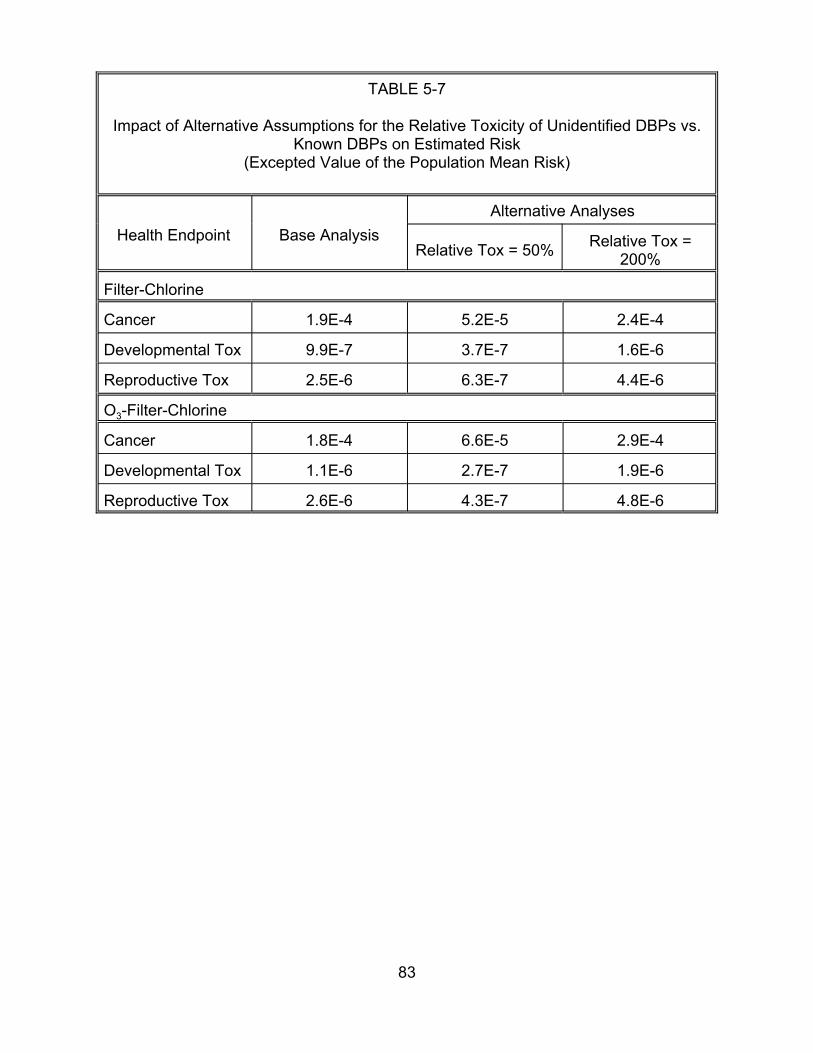
TABLE 5-7
Impact of Alternative Assumptions for the Relative Toxicity of Unidentified DBPs vs. Known DBPs on Estimated Risk
(Excepted Value of the Population Mean Risk)
Health Endpoint Base Analysis Alternative Analyses
Relative Tox = 50% Relative Tox = 200%
Filter-Chlorine
Cancer
Developmental Tox
Reproductive Tox
O3-Filter-Chlorine
Cancer
Developmental Tox
Reproductive Tox
2.4E-4
1.6E-6
4.4E-6
2.9E-4
1.9E-4
9.9E-7
2.5E-6
1.8E-4
5.2E-5
3.7E-7
6.3E-7
6.6E-5
1.1E-6 2.7E-7 1.9E-6
2.6E-6 4.3E-7 4.8E-6
83
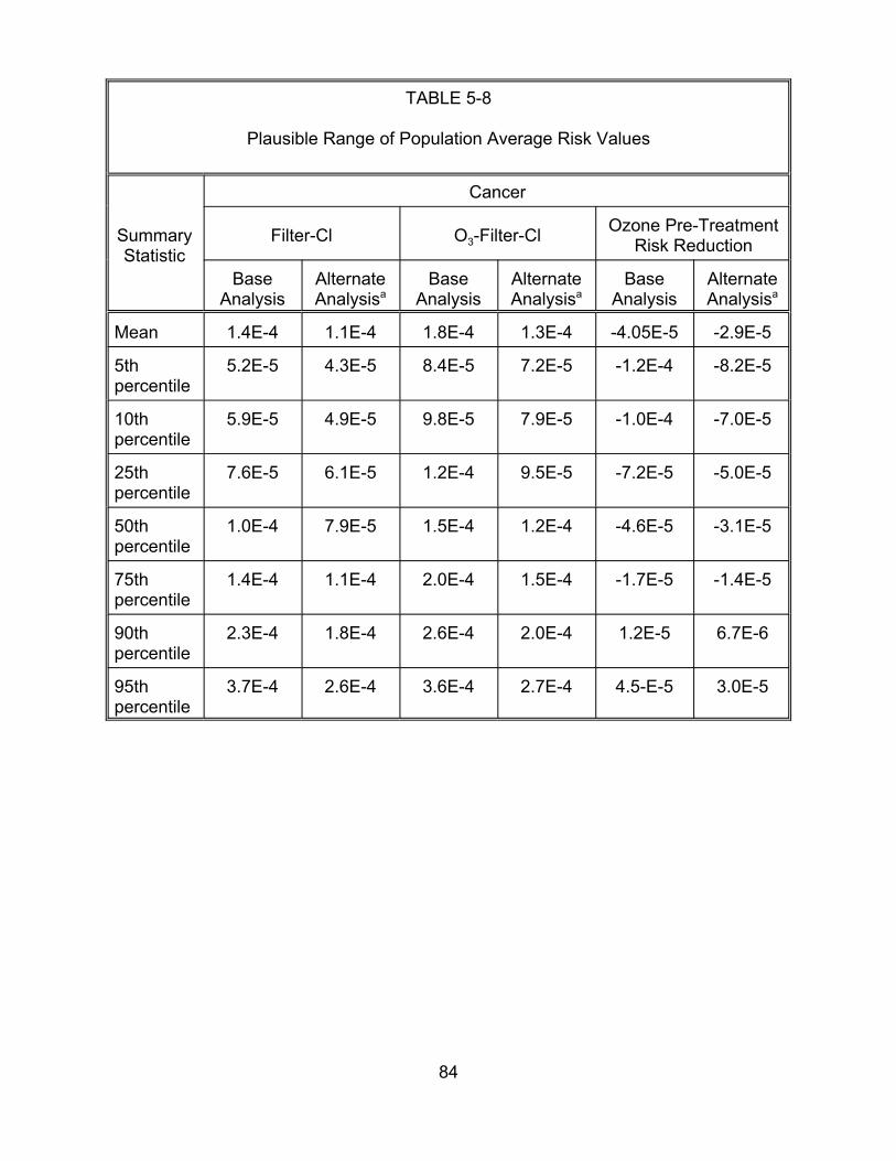
TABLE 5-8
Plausible Range of Population Average Risk Values
Summary Statistic
Cancer
Filter-Cl O3-Filter-Cl Ozone Pre-Treatment Risk Reduction
Base Analysis
Alternate Analysisa
Base Analysis
Alternate Analysisa
Base Analysis
Alternate Analysisa
Mean 1.4E-4 1.1E-4 1.8E-4 1.3E-4 -4.05E-5 -2.9E-5
5th percentile
5.2E-5 4.3E-5 8.4E-5 7.2E-5 -1.2E-4 -8.2E-5
10th percentile
5.9E-5 4.9E-5 9.8E-5 7.9E-5 -1.0E-4 -7.0E-5
25th percentile
7.6E-5 6.1E-5 1.2E-4 9.5E-5 -7.2E-5 -5.0E-5
50th percentile
1.0E-4 7.9E-5 1.5E-4 1.2E-4 -4.6E-5 -3.1E-5
75th percentile
1.4E-4 1.1E-4 2.0E-4 1.5E-4 -1.7E-5 -1.4E-5
90th percentile
2.3E-4 1.8E-4 2.6E-4 2.0E-4 1.2E-5 6.7E-6
95th percentile
3.7E-4 2.6E-4 3.6E-4 2.7E-4 4.5-E-5 3.0E-5
84
although somewhat negative, impact on the overall cancer risk estimate for each of the
two treatment trains considered. It may be noted that the science of chloroform as a
carcinogenic compound and its risk application are controversial and at this time (April,
1999) are undergoing additional external peer review by EPA’s Science Advisory Board.
5.3.2.4. The Assumption that the DBP Slope Factor Distributions are
Statistically Independent — The results in Table 5-9 compare the plausible range of
population average risk values for the base analysis (slope factor estimates statistically
independent) and an alternative analysis (slope factor estimates perfectly correlated for
each health endpoint). For both the filter-Cl treatment train and the O3-filter-Cl
treatment train, the range of plausible values is wider when the slope factor estimates
are assumed to be perfectly correlated. However, the two sets of analyses do not differ
substantially, indicating that this source of uncertainty does not have an important
impact on the results.
85
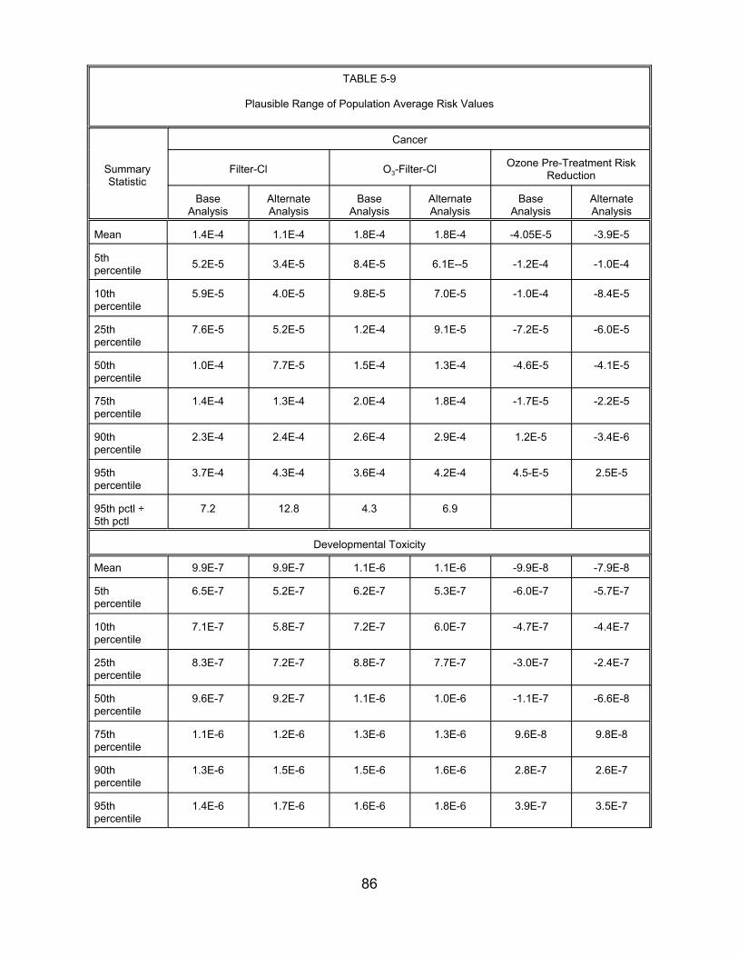
TABLE 5-9
Plausible Range of Population Average Risk Values
Summary Statistic
Cancer
Filter-Cl O3-Filter-Cl Ozone Pre-Treatment Risk Reduction
Base Analysis
Alternate Analysis
Base Analysis
Alternate Analysis
Base Analysis
Alternate Analysis
Mean 1.4E-4 1.1E-4
5th percentile 5.2E-5 3.4E-5
10th percentile
5.9E-5 4.0E-5
25th percentile
7.6E-5 5.2E-5
50th percentile
1.0E-4 7.7E-5
75th percentile
1.4E-4 1.3E-4
90th percentile
2.3E-4 2.4E-4
95th percentile
3.7E-4 4.3E-4
95th pctl ÷ 5th pctl
7.2 12.8
1.8E-4 1.8E-4
8.4E-5 6.1E--5
9.8E-5 7.0E-5
1.2E-4 9.1E-5
1.5E-4 1.3E-4
2.0E-4 1.8E-4
2.6E-4 2.9E-4
3.6E-4 4.2E-4
4.3 6.9
-4.05E-5 -3.9E-5
-1.2E-4 -1.0E-4
-1.0E-4 -8.4E-5
-7.2E-5 -6.0E-5
-4.6E-5 -4.1E-5
-1.7E-5 -2.2E-5
1.2E-5 -3.4E-6
4.5-E-5 2.5E-5
-9.9E-8 -7.9E-8
-6.0E-7 -5.7E-7
-4.7E-7 -4.4E-7
-3.0E-7 -2.4E-7
-1.1E-7 -6.6E-8
9.6E-8 9.8E-8
2.8E-7 2.6E-7
Developmental Toxicity
Mean 9.9E-7 9.9E-7 1.1E-6
5th percentile
6.5E-7 5.2E-7 6.2E-7
10th percentile
7.1E-7 5.8E-7 7.2E-7
25th percentile
8.3E-7 7.2E-7 8.8E-7
50th percentile
9.6E-7 9.2E-7 1.1E-6
75th percentile
1.1E-6 1.2E-6 1.3E-6
90th percentile
1.3E-6 1.5E-6 1.5E-6
95th percentile
1.4E-6 1.7E-6 1.6E-6
1.1E-6
5.3E-7
6.0E-7
7.7E-7
1.0E-6
1.3E-6
1.6E-6
1.8E-6 3.9E-7 3.5E-7
86

TABLE 5-9 cont.
Summary Statistic
Cancer
Filter-Cl O3-Filter-Cl Ozone Pre-Treatment Risk Reduction
Base Analysis
Alternate Analysis
Base Analysis
Alternate Analysis
Base Analysis
Alternate Analysis
95th 2.2 3.3 percentile
Reproductive Toxicity
Mean 2.5E-6 2.6E-6
5th percentile 1.1E-6
10th percentile
1.3E-6
25th percentile
1.7E-6
50th percentile
2.3E-6
75th percentile
3.1E-6
90th percentile
4.0E-6
95th pctl ÷ 5th pctl
4.4
8.5E-7
1.1E-6
1.5E-6
2.2E-6
3.2E-6
4.6E-6
6.7
2.5 3.5
2.6E-6 2.6E-6
1.1E-6 8.6E-7
1.2E-6 1.0E-6
1.7E-6 1.5E-6
2.4E-6 2.3E-6
3.1E-6 3.2E-6
4.3E-6 4.5E-6
4.8 6.5
87
-7.7E-8 7.8E-9
-1.4E-6 -1.3E-6
-1.1E-6 -9.1E-7
-5.4E-7 -4.1E-7
-8.9E-8 9.1E-9
3.9E-7 4.5E-7
9.8E-7 9.4E-7
6. REFERENCES
Bove, F.J., M.C. Fulcomer, J.B. Klotz, J. Esmart, E.M. Dufficy and J.E. Savrin. 1995. Public drinking water contamination and birth outcomes. Am. J. Epidemiol. 141(9):850-862.
Bull, R.J. and F.C. Kopfler. 1991. Health effects of disinfectants and disinfection byproducts. AWWA Research Foundation.
Bull, R.J., M. Robinson, J.R. Meier and J. Stober. 1982. Use of biological assay systems to assess the relative carcinogenic hazards of disinfection by-products. Environ. Health Perspect. 46:215-227.
Cantor, K.P., R. Hoover and P. Hartge et al. 1985. Drinking water source and bladder cancer: A case-control study. In: Water Chlorination: Chemistry, Environmental Impact and Health Effects, Vol. 5.
Cantor, K.P., C.F. Lunch, M. Hildesheim et al. 1997. Drinking water source and chlorination byproducts. I. Risk of bladder cancer. Epidemiololgy. 9:21-28.
CDC (Centers for Disease Control and Prevention). 1995. Assessing the Public Health Threat Associated with Waterborne Cryptosporidiosis: Report of a Workshop. MMWR 44:No.RR-6, June 16, Atlanta, GA 30333.
Christ, S.A., E.J. Read, J.A. Stober and M.K. Smith. 1995. The developmental toxicity of bromochloroacetonitrile in pregnant Long-Evans rats. Internat. J. Environ. Health Res. 5:175-188.
Cicmanec, J.L., L.W. Condie, G.R. Olson and S.-R. Wang. 1991. 90-Day toxicity study of dichloroacetate in dogs. Fund. Appl. Toxicol. 17:376-389.
Cohen, J.T., M.A. Lampson and T.S. Bowers. 1996. The use of two-stage Monte Carlo simulation techniques to characterize variability and uncertainty in risk analysis. Human and Ecological Risk Assessment. 2(4):939-971.
Ershow, A.G., L.M. Brown and K.P. Cantor. 1991. Intake of tapwater and total water by pregnant and lactating women. Am. J. Publ. Health. 81:328-334.
Evans, J.S., G.M. Gray, R.L Sielken, Jr., A.E. Smith, C. Valdez-Flores and J. Graham. 1994. Use of probabilistic expert judgment in uncertainty analysis of carcinogenic potency. Reg. Toxicol. Pharmacol. 20:15-36.
Freedman, M., K.P. Cantor, N.L. Lee et al. 1997. Bladder cancer and drinking water: A population-based case-control study in Washington County, Maryland (United States). Cancer Causes and Control. 8:738-744.
88
Gaylor, D.W., J.A. Axelrad, R.P Brown et al. 1997. Health risk assessment practices in the U.S. Food and Drug Administration. Reg. Toxicol. Pharmacol. 26:307-321.
Gennings, C., P. Schwartz, W.H. Carter, Jr. and J.E. Simmons. 1997. Detection of departures from additivity in mixtures of many chemicals with a threshold model. J. Agric. Biol. Environ. Stat. 2:198-211.
Hoxie, N.J., J.P. Davis, J.M. Vergeront, R.D. Nashold and K.A. Blair. 1997. Cryptosporidiosis-associated mortality following a massive waterborne outbreak in Milwaukee, Wisconsin. Am. J. Publ. Health. 87:2032-2035.
Jacangelo, J.G., N.L. Patania, K.M. Reagan, E.M. Aieta, S.W. Krasner and M.J. McGuire. 1989. Ozonation: Assessing its role in the formation and control of disinfection byproducts. J. AWWA. 81:74-84.
Jo, W.K., C.P. Weisel and P.J. Lioy. 1990a. Chloroform exposure and the health risk associated with multiple uses of chlorinated tap water. Risk Anal. 10 (4): 581-583
Jo, W.K., C.P. Weisel and P.J. Lioy. 1990b. Routes of chloroform exposure and body burden from showering with chlorinated tap water. Risk Anal. 10 (4): 575-579
Juranek, D. 1995. Cryptosporidiosis: Sources of infection and guidelines for prevention. Clin. Infect. Dis. 21(1):S57-61.
Kavlock, R., N. Chernoff, B. Carver and F. Kopfler. 1979. Teratology studies in mice exposed to municipal drinking water concentrates during organogenesis. Fd. Cosmet. Toxicol. 17:343-347.
King, W.D. and L.D. Marrett. 1996. Case-control study of water source and bladder cancer. Cancer Causes and Control. 7:596-604.
Kool, H.J., C.F. van Kreijl and H.J. van Kranen. 1981. The use of XAD-resins for the detection of mutagenic activity in water. II. Studies with drinking water. Chemosphere. 10:99-108.
Kramer, M.D., C.F. Lynch, P. Isacson and J.W. Hanson. 1991. The association of waterborne chloroform with intrauterine growth retardation. Epidemiology. 3(5):407-413.
Krasner, S.W., M.J. McGuire, J.G. Jacangelo, N.L. Patania, K.M. Reagan and E.M. Aieta. 1989. The occurrence of disinfection byproducts in U.S. drinking water. J. Am. Water Works Assoc. 81:41-53.
Linder, R.E., G.R. Klinefelter, L.F. Strader, J.D. Suarez, N.L. Roberts and C.J. Dyer. 1994. Spermatoxoicity of dibromacetic acid in rats after 14 daily exposure. Reprod. Toxicol. 8:251-259.
89
Linder, R.E., G.R. Klinefelter, L.F. Strader, J.D. Suarez and N.L. Roberts. 1997. Spermatotoxicity of dichloroacetic acid. Reprod. Toxicol. 11:681-688.
Loper, J.C., D.R. Lang, R.S. Schoeny, B.B. Richmond, P.M. Gallagher and C.C. Smith. 1978. Residue organic mixtures from drinking water show in vitro mutagenic and transforming activity. J. Toxicol. Environ. Health. 4:919-938.
Lykins, B., R. Clark and J. Goodrich. 1991. Point-of-use/Point-of-entry for Drinking Water Treatment. Lewis Publishers, Boca Raton, Ann Arbor, and London.
Lykins, Jr., B.W., W.E. Koffskey and K.S. Patterson. 1994. Alternative disinfectants for drinking water treatment. J. Environ. Eng. 120(4):745-758.
McGeehin, M.A. et al. 1993. Case-control study of bladder cancer and water disinfection methods in Colorado. Am. J. Epidemiol. 138:492-501.
Miltner, R.J. and R.S. Summers. 1992. A Pilot Scale Study of Biological Treatment. Proceedings, Water Quality, AWWA Annual Conference, Vancouver, BC.
Miltner, R.J., E.W. Rice and A.A. Stevens. 1990. Pilot-Scale Investigation of the Formation and Control of Disinfection Byproducts. In: 1990 Annual Conference Proceedings. AWWA Annual Conference, Cincinnati, Ohio. 2:1787-1802.
Miltner, R.J., E.W. Rice and B.L. Smith. 1992. Ozone's Effect on Assimilable Organic Carbon, Disinfection Byproducts and Disinfection Byproduct Precursors. Proceedings, AWWA, WQTC, Orlando, FL.
Morris, R.D., A-M. Audet, I.F. Angelillo, T.C. Chalmers and F. Mosteller. 1992. Chlorination, chlorination by-products, and cancer: A meta-analysis. Am. J. Public Health. 82:955-963. (Erratum: Am. J. Public Health. 83:1257.)
Mumtaz, M. and R.C. Hertzberg. 1993. The status of interactions data in risk assessment of chemical mixtures. In: Hazard Assessment of Chemicals, J. Saxena, Ed. Hemisphere Publishing Corporation, Washington, DC. 8:47-79.
Narotsky, M.G., R.A. Pegram and R.J. Kavlock. 1997. Effect of dosing vehicle on the developmental toxicity of bromodichloromethane and carbon tetrachloride in rats. Fund. Appl. Toxicol. 40:30-36.
National Center for Health Statistics. 1997. Health, United States 1996-1997. Public Health Service, Hyattsville, MD.
Nestman, E.R., R. Otson, G.L. LeBel, D.T. Williams, E.G.H. Lee and D.C. Biggs. 1982. Correlation of water quality parameters with mutagenicity of drinking water extracts. In: Water Chlorination: Environmental Impact and Health Effects, Vol. 4, R.L. Jolley, W.A. Brungs and R.B. Cumming, Ed. Ann Arbor Science Publ., Ann Arbor, MI.
90
NTP (National Toxicology Program). 1985. Toxicology and carcinogenesis studies of chlorodibromomethane in F344/N rats and B6C3F mice (gavage studies). NTP TR282.
NTP (National Toxicology Program). 1986. Toxicology and carcinogenesis studies of bromodichloromethane in F344/N rats and B6C3F mice (gavage studies). NTP Technical Report, Ser. No. 321, NIH Publ. No. 87-2537.
NTP (National Toxicology Program). 1989. Toxicology and carcinogenesis studies of tribromomethane and bromoform in F344/N rats and B6C3F mice (gavage studies). NTP-350.
Pereira, M.A. and J.B. Phelps. 1996. Promotion by dichloroacetic acid and trichloroacetic acid of N-methyl-N-nitrosourea-initiated cancer in the liver of female B6C3F1 mice. Cancer Lett. 102:133-141.
Perz, J.F., F.K. Ennever and S.M. Le Blancq. 1998. Cryptosporidium in tap water. Comparison of predicted risks with observed levels of disease. Am. J. Epidemiol. 147:289-301.
Randall, J.L., S.A. Christ, P. Horton-Perez, G.A. Nolen, E.J. Read and M.K. Smith. 1991. Developmental effects of 2-bromacetic acid in the Long-Evans rat. Teratology. 43:454.
Richardson, S.D. 1998. Identification of drinking water disinfection by-products. In: Encyclopedia of Environmental Analysis and Remediation, R.A. Meyers, Ed. Wiley and Sons. 3:1398-1421.
Ries, L.A.G., C.L. Kosary, B.F. Hankey, B.A. Miller and B.K. Edwards. 1998. SEER Cancer Statistics Review, 1973-1995, National Cancer Institute. Bethesda, MD. (PDF Electronic file)
Shukairy, H.M., R.J. Miltner and S.R. Summers. 1994. Bromide's effect on DBP formation, speciation and control: Part I, Ozonation. J. AWWA. 86(6):72-87. June.
Singer, S. 1997. RO: New thinking on countering biological risks. Water Conditioning and Purification. July.
Smith, M.K., J.L. Randall, D.R. Tocco, R.G. York, J.A. Stober and E.J. Read. 1988. Teratogenic effects of trichloroacetonitrile in the Long-Evans rat. Teratology. 38:113-120.
Smith, M.K., J.L. Randall, E.J. Read and J.A. Stober. 1989a. Teratogenic activity of trichloroacetic acid in the rat. Teratology. 40:445-451.
Smith, M.K., J.L. Randall, J.A. Stober and E.J. Read. 1989b. Developmental toxicity of dichloroacetonitrile: A by-product of drinking water disinfection. Fund. Appl. Toxicol. 12:765-772.
91

Smith, M.K, J.L. Randall, E.J. Read and J.A. Stober. 1990. Developmental effects of chloroacetic acid in the Long-Evans rat. Teratology. 41:593.
Smith, M.K., J.L. Randall, E.J. Read and J.A. Stober. 1992. Developmental toxicity of dichloracetate in the rat. Teratology. 46:217-223.
Swan, S.H., K. Waller, B. Hopkins et al. 1998. A prospective study of dpontaneous abortion: Relation to amount and source of drinking water consumed in early pregnancy. Epidemiology. 9(2):126-133.
U.S. EPA. 1986. Guidelines for the Health Risk Assessment of Chemical Mixtures. Federal Register. 51(185):34014-34025.
U.S. EPA. 1989. Risk Assessment Guidance for Superfund, Vol. 1, Part A. EPA/540/1-89/002.
U.S. EPA. 1990. Technical Support Document on Health Risk Assessment of Chemical Mixtures. EPA/600/8-90/064.
U.S. EPA. 1995. Policy for Risk Characterization at the U.S. Environmental Protection Agency. Memorandum from Carol Browner, March 21, 1995.
U.S. EPA. 1996. Proposed Guidelines for Carcinogen Risk Assessment; notice. Federal Register. 61(79):17961-18011.
U.S. EPA. 1997. Exposure Factors Handbook. Volume 1. General Factors. Office of Research and Development, National Center for Environmental Assessment. EPA/600/P-95/002Fa. August.
U.S. EPA. 1998a. Comparative Risk Framework Methodology. National Center for Environmental Assessment, Cincinnati, OH. Online. http://www.epa.gov/ncea/frame.htm
U.S. EPA. 1998b. National Primary Drinking Water Regulations; Disinfectants and Disinfection By-Products Notice of Data Availability; Proposed Rule. 40 CFR parts 141 and 142. Fed. Reg. 63(61):15674-15692.
U.S. EPA. 1998c. Comparative Risk Framework Methodology and Case Study. SAB External Review Draft. NCEA-C-0135.
U.S. EPA. 1998d. Workshop Report: The Risk Assessment of Mixtures of Disinfection By-Products (DBPs) in Drinking Water. NCEA-C-0459.
U.S. EPA. 1998e. Guidance for Conducting Health Risk Assessment of Chemical Mixtures. Internal Review Draft. NCEA-C-0148.
92

U.S. EPA. 2000. Integrated Risk Information System (IRIS). Online. National Center for Environmental Assessment, Washington, DC.
Waller, K., S.H. Swan, G. DeLorenze and B. Hopkins. 1998. Trihalomethanes in drinking water and spontaneous abortion. Epidemiology. 9(2):134-140.
93
APPENDIX A
EPA Pilot-Scale Investigation of the Formation and Control of Disinfection Byproducts
PILOT-SCALE INVESTIGATION OF THE FORMATION AND CONTROLOF DISINFECTION BYPRODUCTS
Richard J. Miltner, P.E.Eugene W. RiceAlan A. Stevens
Drinking Water Research DivisionU.S. Environmental Protection Agency
Cincinnati, Ohio 45268
Ozone's role in water treatment in the USA is increasing for a number of reasons. It is a powerful disinfectant, resulting in lower C-t (concentration x time) requirements than chlorine, chlorine dioxide or chloramines. It will not form trihalomethanes (THMs), except in the case of high bromide in the source water. It will react with THM precursors, under appropriate conditions, to lower THM formation potential (THMFP). It can also enhance the flocculation of particulates, improve taste and odor, remove color, and control iron and manganese.
Maximum contaminant levels (MCLs) of THMs will likely be lowered in 1991 under the Disinfection-Disinfection Byproducts (D-DBP) Rule. The 1986 Amendments to the Safe Drinking Water Act require that the EPA regulate new contaminants beginning in 1991. Candidate contaminants are given in the Drinking Water Priority List (DWPL) and include THMs, numerous other halogenated DBPs and ozone byproducts. The DWPL and a summary of the D-DBP Rule are given in the Journal AWWA (1).
This study, which was conducted by EPA's Drinking Water Research Division (DWRD), examined byproduct formation and control in three parallel pilot plants employing conventional treatment of Ohio River water. In one plant, chlorine was applied following filtration, allowing conventional treatment to remove precursor materials. In a second plant, chlorine was also applied following filtration, but ozone was applied to the raw water to enhance precursor control. In a third plant, monochloramine was applied to filtered water with ozone applied to raw water. The DBPs that were studied are given in Table 1.
Analytic methods for the ozone byproducts and for several of the non-THM halogenated DBPs in Table 1 are under development. The methods and sample preservatives used in this study are given in the Journal AWWA (2-4).
A.1-1
HALOGENATED DBP SAMPLING
Samples were collected for both instantaneous and terminal total trihalomethanes (inst TTHM and term TTHM). In the terminal sample the THM reaction is driven to completion thereby exhausting the precursor material that is present and forming the highest concentration of THMs. In this study, term TTHM concentrations occurred when samples were taken from the pilot plants and chlorinated on the bench with 12 mg/L added chlorine and stored headspace-free, in the dark, for seven days, at 25°C. The pH was that of the pilot plant finished water, i.e., near 8.1. Free chlorine residuals were present after seven days to ensure that the reactions were not chlorine limited. For any sample, the unreacted precursor is represented by the THMFP which is the difference between the term TTHM and the back-ground or inst TTHM. The term TTHM and the THMFP allow an assessment of the control of precursor during treatment. This approach to THM sampling is described in detail by Stevens and Symons (5).
For compliance with MCLs, distribution system inst TTHM is important. In this study, the inst TTHM in a simulated distribution system (SDS TTHM) was determined by storing finished water samples in the dark, at 25°C, headspace-free, for three days, without added chlorine. Chlorine or chloramine was applied according to the Ten States Standards (TSS) (6); residuals after three days were near 0.2 mg/L free chlorine or 0.7 mg/L monochloramine.
Because of limited analytic resources, term TTHM samples were not collected at each sample point, but only for raw, settled and finished waters, as previous studies indicated that most removal of precursor occurred with sedimentation and that little additional removal occurred with filtration (7).
Instantaneous and SDS samples were collected for all halogenated DBPs, Terminal samples were not collected for haloacetonitriles, 1,1,1-tri-chloroporopanone or chloral hydrate because those byproducts are not stable for seven days near pH 8 (2), or for cyanogen chloride because it is not stable in the presence of free chlorine.
PILOT-SCALE FACILITIES
DWRD's pilot plants and its counter-current ozonation chamber are described in detail elsewhere (8). These parallel plants were operated continuously for one week. Following start-up and the establishment of steady-state operation, samples were collected daily. Sample points were selected to isolate unit processes and are indicated by circles in Figure 1.
A.1-2
For this study, mean values are reported. Temperatures in pilot plant waters ranged from 26 to 28°C. pH ranged from 7.4 to 8.1. Raw water turbidity ranged from 9 to 20 Ntu; settled water turbidity averaged 1.6 Ntu; filtered water turbidities were less than 0.18 Ntu. Each filter was backwashed with water from its dedicated clear well. Backwashing occurred near 30 inches head loss (every three days approximately) and followed TSS practices. To apply chlorine, calcium hypochlorite was added. To apply monochloramine, calcium hypochlorite and ammonium hydroxide were added in that order ahead of in-line mixers in series. The ammonia was added in stoichiometric excess. Samples taken immediately downstream of the two in-line mixers showed only traces of free chlorine.
Mean ozonation conditions are given in Table 2. An applied ozone-to-TOC ratio of 0.8 was chosen as representative of conditions typically employed in Europe as a pre-oxidant. At the time of this study, the DPD method was used to determine dissolved ozone residuals. Mean residuals effluent from the contactor and mix tank were 0.47 and 0.14 mg/L, respectively. No ozone was detected in the floc tank effluent.
MICROBIOLOGICAL SAMPLING
Bacteria and phage were spiked into raw water to increase microbiological densities to approximately 4 logs so as to monitor their control through the various unit processes. Total coliform (TC) and heterotrophic plate count (HPC) bacteria were added as primary sewage (1 to 1,000 dilution). As viral indicators, MS-2 phage were added via in-line mixer. Assimilable organic carbon (AOC) was monitored, following the procedure of van der Kooij, et al (9), to assess the effect of ozone on conversion of natural organic matter (NOM) to materials assimilable by heterotrophs that could potentially cause regrowth:problems in distribution systems. Similarly, coliform growth response (CGR) was monitored, following the procedure, of Rice (10), to assess the effect of ozone on materials assimilable by coliforms.
RESULTS AND DISCUSSION
Halogenated DBPs
Using TOX as a surrogate for halogenated DBPs, comparative formation and control may be seen in Figure 2, where data representing the three parallel plants are given. Approximately 19 percent of the precursor material was removed (comparing mean terminal concentrations of 521 and 421 :g Cl/L) by conventional treatment. With ozone applied ahead of conventional treatment, 27 percent of the precursor was removed;
A.1-3
however, removal in this case must be considered as both the separation of precursor as a result of coagulation and clarification and the oxidation of precursor as a result of ozonation. Because these data represent mean values over a week's operation, the difference in means of settled waters were t-tested. At the 95 percent confidence level, the means were not different suggesting that ozone's effect on precursor control, at the ozone conditions selected, was not significant. Further t-testing indicated that, for most compounds, apparent changes in precursor from settled water, through filtration, to clear well storage were insignificant at the 95 percent confidence level. In Figure 2, for example, there was no difference, statistically, in mean term TOX concentrations of 421 and 440 ug Cl/L for waters that were pre-ozonated. Data on control of precursor for TOX and other parameters are presented in Table 3, and similarly suggest that ozone's effect on precursor was not significant for TOC or for specific halogenated DBPs. Indeed, for the more heavily brominated DBPs and for chloropicrin, ozone's effect is detrimental, as will be discussed. (In Table 3, data from the two chlorinated plants were statistically tested.)
Tables 4 and 5 present mean DBP concentrations from the three pilot plants and statistical tests of data from the two plants applying chlorine. These tables reveal much about the formation and control of halogenated DBPs:
(1) The use of ozone and chloramine resulted in the lowest formation of halogenated DBPs because free chlorine was not present to drive these reactions. The only exception to this was cyanogen chloride which was not detected until monochloramine was applied.
(2) When free chlorine was applied, concentrations were higher in SDS water (3-day stored) than in finished water (clear well) indicating that as long as a residual is present and precursor has not been exhausted, concentrations will continue to increase. This increase in instantaneous concentration may be seen in Figure 2 for TOX and in Figure 3 for chloroform. These figures both indicate sufficient precursor remaining in finished water to react with residual chlorine. 1,1,1-Trichoropropanone was the exception in this case. Its instability near pH 8 at 25°C over three days accounts for the decrease, as seen in Figure 4.
(3) When monochloramine was applied, concentrations in finished and SDS waters were statistically the same for most halogenated DBPs. Exceptions were cyanogen chloride, as noted, 1,1,1-trichlaropropanone (Figure 4), and chloral hydrate. Clearly, monochloramin drives these reactions, but factors effecting the formation of these non-THM DBPS are not well understood and require research.
A.1-4
(4) On a weight basis, the haloacetic acids account for more halogenated DBP production than other compounds, with the exception of THMs. Table 6 converts each halogenated DBP to its TOX equivalent, i.e., as ug Cl/L, and illustrates that the haloacids and the THMs comprise more than three-fourths of accounted-for TOX. It is interesting to note that over half the TOX remains unaccounted for; therefore, analytic means to elucidate other halogenated DBPs remain a research priority.
(5) Although differences in precursor control were small with and without ozonation and not significant at the 95 percent confidence level (Table 3), changes in precursor were apparent when examining differences in instantaneous DBPs found in chlorinated finished and SDS waters (Tables 4 and 5). In the SOS water that was ozonated, the mean chloroform concentration was 39.6 ug/L, while in the parallel water that was not ozonated, the mean concentration was 55.5 ug/L. Figure 3 illustrates this advantage of ozonation for chloroform. Results of statistical tests in Tables 4 and 5 show that (a) this advantage holds for other more heavily chlorinated DBPs, i.e., di- and trichloroacetic acid, (b) the effects of ozonation can not be statistically differentiated for many of the DBPs, and (c) for the more heavily brominated DBPs and for chloropicrin, ozonation results in more, rather than less, DBP formation. This advantage of ozone on the formation of the more heavily chlorinated DBPs is seen in Figure 3 for chloroform and in Figure 5 for dichloroacetic acid. The disadvantage of ozone in the case of the more heavily brominated DBPs is seen in Figure 6 for dibromochloromethane and in Figure 7 for dibromoacetic acid. In the case of dibromoacetic acid, the precursor increased 26 percent (comparing mean terminal concentrations of 1.39 and 1.5 ug/L), as seen in Figure 7 and Table 3, and continued to increase in downstream Processes. This increase in precursor is not well understood. The THM reaction will proceed more rapidly when driven by bromine (which is converted from bromide by chlorine) than when driven by chlorine. Note in Figures 6 and 7 that the concentrations of these more heavily brominated DBPs in 3-day stored waters reached those of the raw water THMFP when chlorine alone was used. However, in Figures 3 and 5, the concentrations of the more heavily chlorinated DBPs in 3-day stored waters did not reach those of their raw water THMFP when chlorine alone was used because the chlorine-driven reactions are slower. Conversely, in Figures 6 and 7 the concentrations of the more heavily brominated DBPs in 3-day stored waters where both ozone and chlorine were used exceeded those of the raw water THMFP. Perhaps intermediate oxybromine species were created in the ozone contactor that continued to slowly increase the precursor concentration in downstream processes in the absence of an ozone residual. Another contributing factor may be the change in the bromine-to-chlorine ratio. As will be discussed, ozone lowered the chlorine demand thereby increasing this ratio on the
A.1-5
ozone/chlorine plant. This would favor the formation of the more heavily brominated DBPs. The conversion by ozone of bromide to bromine that would rapidly drive the THM or haloacid reaction does not appear to be significant because no increase in either inst dibromochloromethane (Figure 6) or inst dibromoacetic acid (Figure 7) was observed in ozonated and settled waters. The detrimental effect of ozone on precursor in the presence of bromide appears to be significant and needs to be studied.
(6) The precursor to the chloropicrin reaction also increased significantly upon ozonation. It continued to increase in downstream processes after the dissolved ozone residual had dissipated. See Figure 8. The concentration in the 3-day stored water exceeded the raw water THMFP in the plant where preozonation occurred. This behavior is likely related to the nitrogenous nature of the chloropicrin's precursor material and ozone's reaction with this material. This was discussed by Hoigne and Bader (11).
(7) Ozonation lowered the chlorine demand of the water. On the plant were chlorine only was applied, a mean dose of 3.04 mg/L was sufficient to carry a 3-day mean residual of 0.2 mg/L; on the ozone/chlorine plant, a mean dose of only 2.82 mg/L was required to carry the same residual. The effect of chlorine dose on the formation of many of these halogenated DBPs is not well known. Therefore, the lower concentrations of inst DBPs observed on the ozone/chlorine plant, compared to the chlorine-only plant, may be due to the lower chlorine dose and/or ozone's effect on precursor as discussed previously.
Microbiological Parameters
On the plants where ozone was employed, significant reduction in bacterial and phage densities took place in the contactor. Figure 9 describes microbiological control on the plant employing ozone and monochloramine. Bacterial counts were higher in finished waters when chloramine was applied (Figure 9) than when chlorine was applied. Ozone brought about approximately two-and-one-half log reductions in both TC and HPC. No MS-2 phage were detected in the effluent from tile contactor, indicating greater than a three-and-one-half log reduction of that viral indicator. This single counter-current contactor would be similar to the first chamber in a full-scale, multi-chambered contactor. It is interesting to note that current language in the Surface Water Treatment Rule (SWTR) allows no credit for viral or Giardia disinfection in a first chamber, assuming that ozone is being used in that chamber to satisfy demand (12). These data suggest that language is too restrictive. It is also interesting to note that counts of surviving heterotrophs significantly increased downstream of the ozone contactor. It is assumed that they utilized the lower molecular weight, easily assimilable NOM produced from the reaction between
A.1-6
ozone and higher molecular weight NOM. Both filtration and post disinfection provided control of heterotrophs. Coliforms surviving the ozone contactor apparently utilize different materials; consequently, their counts decreased through conventional treatment.
On the plant employing chlorination only, conventional treatment lowered TC, HPC and MS-2 phage densities approximately two logs. Post-chlorination lowered the densities of all three parameters to their detection levels.
Ozone Byproducts
The production of formaldehyde is seen in Figure 10. Upon ozonation, mean formaldehyde concentrations reached 26.3 ug/L. Concentrations subsequently declined through conventional treatment but were boosted again upon either clear well chlorination or chloramination. Figure 11 illustrates similar behavior of acetone and glyoxal to that of formaldehyde on the ozone/chlorine plant. Glaze, et al. (13,14) discussed possible mechanisms for the formation of aldehydes upon ozonation. Chlorine's ability to produce formaldehyde was also seen on the plant employing chlorination only.
The loss of formaldehyde, acetone and glyoxal during conventional treatment is assumed to be due to biodegradation by bacteria represented by the HPC. This is described on the ozone/chlorine plant in Figure 12 wherein the decline in formaldehyde concentration through flocculation and sedimentation is matched by an increase in HPC densities. Since formaldehyde is common to both Figures 11 and 12, acetone and glyoxal are, like formaldehyde, assumed to be utilized by the bacteria.
Figure 12 also plots AOC and illustrates that it correlates well with formaldehyde concentrations, therefore, with acetone and glyoxal concentrations also. The bacteria apparently utilizing the aldehydes and ketone as nutrients are doing the same with AOC. Indeed, AOC was developed as a tool to measure bacterial regrowth potential in distribution systems (9). It is clear that increases in AOIC upon ozonation should be controlled in the treatment plant before release to the distribution system, and that optimizing bioactivity in the processes downstream of the ozone contactor is a prudent approach. In this study, concentrations of AOC, aldehydes and ketones were apparently biodegraded in the filter. The filter was backwashed with chlorinated water from its clear well. While sufficient samples of AOC and HPC were not collected to confirm this, it appears that the periodic exposure to chlorine was either not sufficient to destroy bioactivity on the filter, or the filter reestablished its bioactivity quickly following backwashing as it was again exposed to HPC bacteria received
A.1-7
from the settled water. The detrimental effect of backwashing biological filters with disinfected water needs to be studied.
Coliform growth response attempts to measure the regrowth potential of coliforms in the same manner that AOC attempts to measure the regrowth potential of heterotrophs. Figure 12 shows that CGR and AOC correlated well through the ozone/chlorine plant indicating that the CGR enhanced by ozonation was also biodegraded. With post chlorination, however, their behavior was different. AOC increased. with chlorination suggesting regrowth potential for species like Pseudomonas fluorescens, P-17, on which the parameter is based (9). The increase in AOC with clear well chlorination, to near 200 ug/L Ceq/L, is unusually high compared with similar data (10). The CGR decreased with chlorination suggesting no coliform regrowth potential.
REFERENCES
1. F.W. PONTIUS, “Complying with the New Drinking Water Quality Regulations”, J.AWWA, 82:2:32 (February 1990).
2. A.A. Stevens, et al, “Formation and Control of Non-Trihalo-methane Disinfection Byproducts”, J.AWWA, 81:8:54 (August 1989)
3. S.J. KRASNER, et al, “Occurrence of Disinfection Byproducts in US Drinking Water”, J.AWWA, 81:8:41 (August 1989).
4. J.G. JACANGELO, et al, “Ozonation: Assessing Its Role in the Formation and Control of Disinfection Byproducts", J.AWWA, 81:8:74 (August 1989).
5. A.A. STEVENS and J. M. SYMONS, "Measurement of Trihalomethanes and Precursor Concentration Changes”, J.AWWA 69:546 (1977).
6. “Recommended Standards for Water Works”, Committee of the Great Lakes-Upper Mississippi River Board of State Sanitary Engineers, Health Research, Inc., Albany, NY (1987).
7. R.J. MILTNER, “Treatment for Control of Disinfection Byproducts”, Proceedings, Seminar on Current Research Activities in Support of USEPA's Regulatory Agenda, AWWA Annual Conference (June 19, 1990).
8. R.J. MILTNER, et al, “A Study of Ozone's Role in Disinfection Byproduct Control”, Proceedings, Conference on Ozone in Water and Wastewater Treatment, International Ozone Association (March 27-29, 1990).
9. D. VAN DER KOOIJ, et al, “Determining the Concentration of Easily Assimilable Organic Carbon in Drinking Water”, J.AWWA, 74:10:540 (1982).
10. E.W. RICE, et al, 'Bioassay Procedures for Predicting Coliform Bacterial Growth in Drinking Water”, Env. Techno., in press (1990).
A.1-8
11. J. HOIGNE and H. BADER, “Formation of Chloropicrin and Chloroform in a Combined Ozonation/Chlorination Treatment of Drinking Water”, Water Res., 22:3:313 (1988).
12. "Guidance Manual for Compliance with the Filtration and Disinfection Requirements for Public Water Systems Using Surface Water Sources”, USEPA, Office of Drinking Water, Washington, DC (October 1989).
13. W.H. GLAZE, et al, “Application of Closed Loop Stripping and XAD Resin Adsorption for the Determination of Ozone Byproducts from Natural Water”, in Biohazards in Drinking Water Treatment, R. A. Larson, ed., Lewis Publishers, Chelsea, MI (1988).
14. W.H. GLAZE, et al, “Ozonation Byproducts 2. Improvement of an Aqueous-Phase Derivitization Method for the Detection of Formaldehyde and Other Carbonyl Compounds Formed by the Ozonation of Drinking Water”, Env. Sci. Tech., 23:7:838 (July -1989).
A.1-9
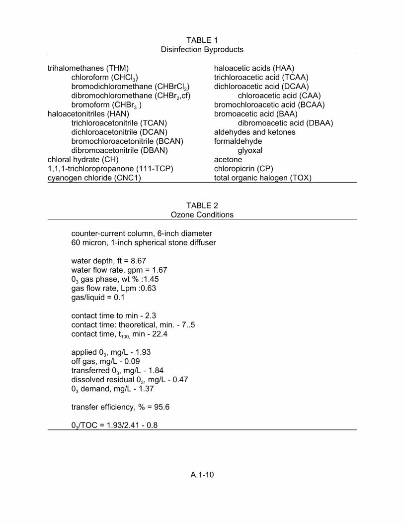
trihalomethanes (THM) chloroform (CHCl3)
TABLE 1 Disinfection Byproducts
haloacetic acids (HAA) trichloroacetic acid (TCAA)
bromodichloromethane (CHBrCl2) dichloroacetic acid (DCAA) dibromochloromethane (CHBr2,cf) chloroacetic acid (CAA) bromoform (CHBr3 ) bromochloroacetic acid (BCAA)
haloacetonitriles (HAN) bromoacetic acid (BAA) trichloroacetonitrile (TCAN) dibromoacetic acid (DBAA) dichloroacetonitrile (DCAN) aldehydes and ketones bromochloroacetonitrile (BCAN) formaldehyde dibromoacetonitrile (DBAN) glyoxal
chloral hydrate (CH) acetone1,1,1-trichloropropanone (111-TCP) chloropicrin (CP)cyanogen chloride (CNC1) total organic halogen (TOX)
TABLE 2Ozone Conditions
counter-current column, 6-inch diameter60 micron, 1-inch spherical stone diffuser
water depth, ft = 8.67water flow rate, gpm = 1.6703 gas phase, wt % :1.45gas flow rate, Lpm :0.63gas/liquid = 0.1
contact time to min - 2.3contact time: theoretical, min. - 7..5contact time, t100, min - 22.4
applied 03, mg/L - 1.93off gas, mg/L - 0.09transferred 03, mg/L - 1.84dissolved residual 03, mg/L - 0.4703 demand, mg/L - 1.37
transfer efficiency, % = 95.6
03/TOC = 1.93/2.41 - 0.8
A.1-10

Table 3
PRECURSOR CONTROL
COMPOUND
PERCENT REMOVAL T-TEST
O3/NH2C1 O3/NH2C12 POST C12 BETTER WITH O3
SAME BETTER WITHOUT O3
TOC
TOX
TTHM CHCI3 CHBrCI2 CHBr2CI
CP
TOTAL HAA TCAA DCAA CAA BCAA DBAA
20
27
33 39 20
--31
-53
30 24 35 18 21 -26
20
27
33 39 20 -31
-53
30 24 35 18 21 -26
11
19
30 33 25 -11
31
21 11 29 18 11 -13
X
X
X X X
X X X X X
X
X
X
- At 95 percent confidence level
Table 4
DBP FORMATION IN FINISHED WATERS
COMPOUND ATION ug/L T-TEST
O3/NH2C1 O3/NH2C12 POST C12 BETTER WITH O3
SAME BETTER WITHOUT O3
TTHM CHCl3 CHBrCl2 CHBr2Cl CHBr3
TOTAL HAN DCAN TCAN BCAN DBAN
111 – TCP CP CH CNCI TOTAL HAA TCAA DCAA CAA BCAA BAA DBAA
5.0 4.2 0.6 0.1 ND 3.3 2.8 ND 0.3 0.3 0.1 ND ND 1.6 3.6 1.5 1.7 0.2 0.2 0.1 ND
32.8 13.0 10.3 9.2 0.3 3.2 1.9 0.1 0.6 0.7 2.4 0.6 2.0 ND 19.6 5.3 8.0 0.7 3.9 0.2 1.6
55.2 30.4 17.6 7.0 ND 3.8 2.4 ND 1.0 0.4 2.1 0.1 3.2 ND 36.0 11.8 17.0 0.7 5.3 0.2 1.0
X X X
X X X
X
X X X X X X X
X
X
X
X
X
X
FORM
AT 95% CONFIDENCE LEVELND-NOT DETECTED
A.1-11
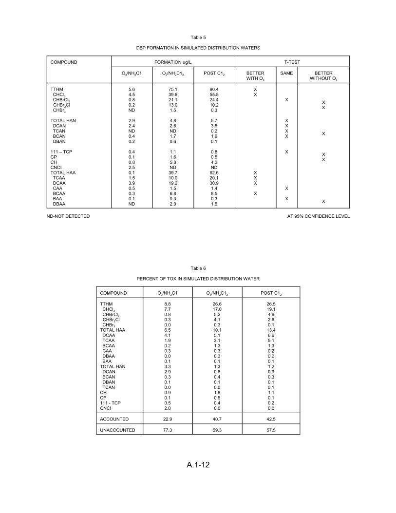
Table 5
DBP FORMATION IN SIMULATED DISTRIBUTION WATERS
COMPOUND ATION ug/L T-TEST FORM
O3/NH2C1 O3/NH2C12 POST C12 BETTER WITH O3
SAME BETTER WITHOUT O3
TTHM CHCl3 CHBrCl2 CHBr2Cl CHBr3
TOTAL HAN DCAN TCAN BCAN DBAN
111 – TCP CP CH CNCI TOTAL HAA TCAA DCAA CAA BCAA BAA DBAA
5.6 4.5 0.8 0.2 ND
2.9 2.4 ND 0.4 0.2
0.4 0.1 0.8 2.5 0.1 1.5 3.9 0.5 0.3 0.1 ND
75.1 39.6 21.1 13.0 1.5
4.8 2.6 ND 1.7 0.6
1.1 1.6 5.8 ND 39.7 10.0 19.2 1.5 6.8 0.3 2.0
90.4 55.5 24.4 10.2 0.3
5.7 3.5 0.2 1.9 0.1
0.8 0.5 4.2 ND 62.6 20.1 30.9 1.4 8.5 0.3 1.5
X X
X X X
X
X
X X X X
X
X
X
XX
X
X X
X
ND-NOT DETECTED AT 95% CONFIDENCE LEVEL
Table 6
PERCENT OF TOX IN SIMULATED DISTRIBUTION WATER
COMPOUND 3/NH2C1 O3/NH2C12 POST C12
TTHM CHCl3 CHBrCl2 CHBr2Cl CHBr3
TOTAL HAA DCAA TCAA BCAA CAA DBAA BAA
TOTAL HAN DCAN BCAN DBAN TCAN
CH CP 111 - TCP CNCI
8.8 7.7 0.8 0.3 0.0 6.5 4.1 1.9 0.2 0.3 0.0 0.1 3.3 2.9 0.3 0.1 0.0 0.9 0.1 0.5 2.8
26.6 17.0 5.2 4.1 0.3 10.1 5.1 3.1 1.3 0.3 0.3 0.1 1.3 0.8 0.4 0.1 0.0 1.8 0.5 0.4 0.0
26.5 19.1 4.8 2.6 0.1 13.4 6.6 5.1 1.3 0.2 0.2 0.1 1.2 0.9 0.3 0.1 0.1 1.1 0.1 0.2 0.0
ACCOUNTED 22.9 40.7 42.5
O
UNACCOUNTED 77.3 59.3 57.5
A.1-12
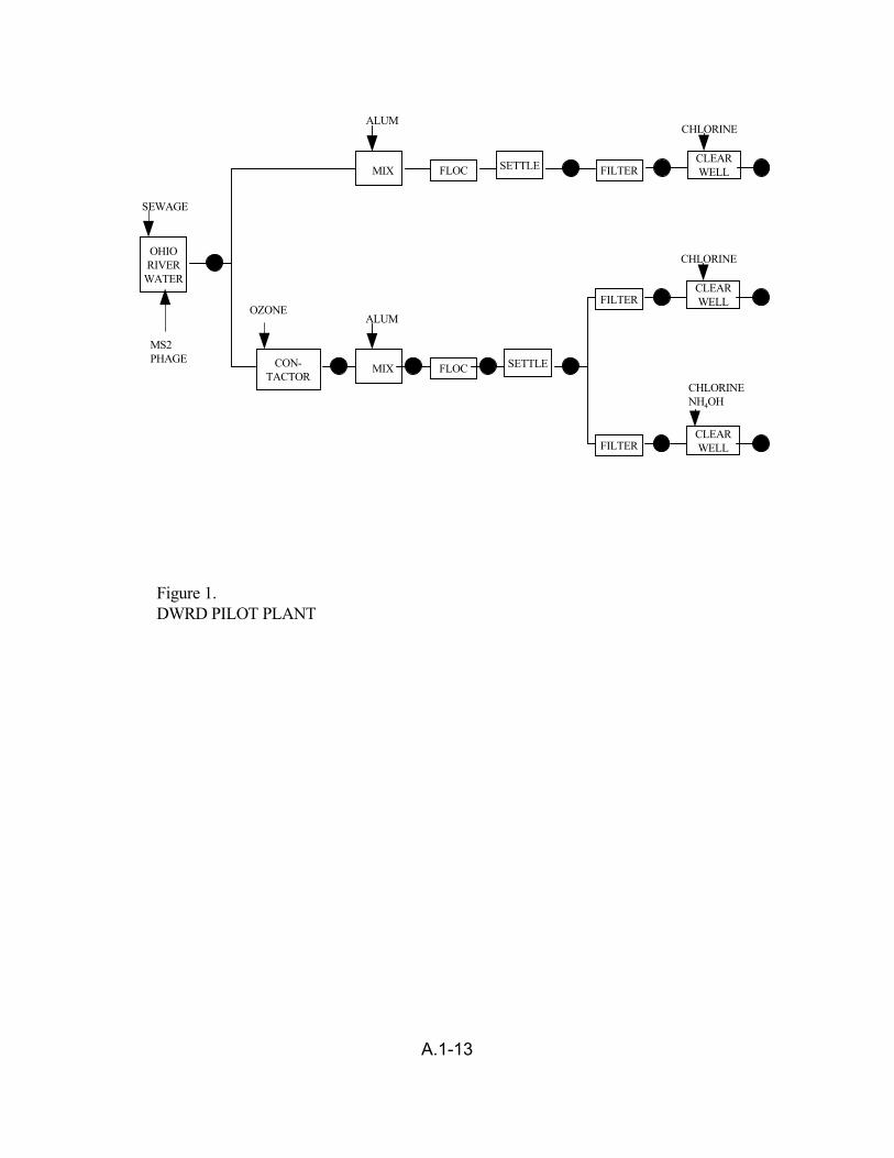
ALUM CHLORINE
CLEAR WELL
SEWAGE
OHIO RIVER
WATER
FLOC FILTER
CON-TACTOR
MIX
OZONE
SETTLE
FILTER
FILTER
FLOC MIX
ALUM
SETTLE
CHLORINE
CLEAR WELL
MS2 PHAGE
CHLORINE NH4OH
CLEAR WELL
Figure 1.DWRD PILOT PLANT
A.1-13
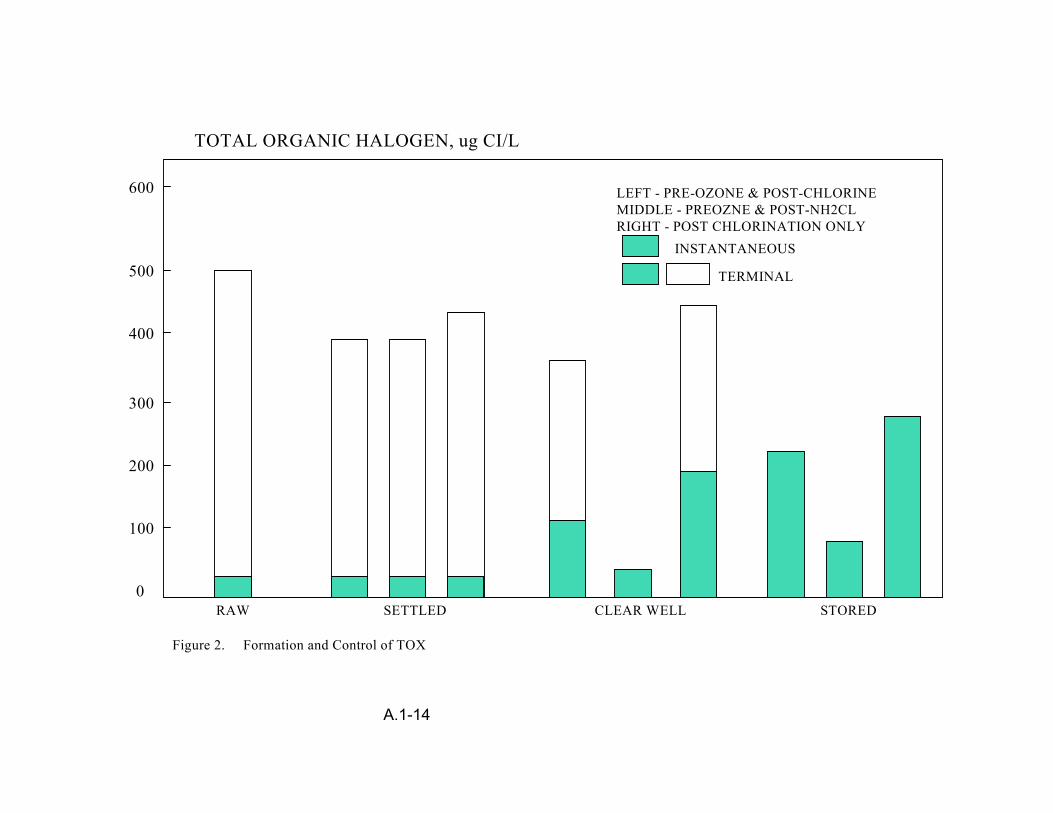
TOTAL ORGANIC HALOGEN, ug CI/L
600
500
400
300
200
100
0 RAW SETTLED CLEAR WELL STORED
LEFT - PRE-OZONE & POST-CHLORINE MIDDLE - PREOZNE & POST-NH2CL RIGHT - POST CHLORINATION ONLY
INSTANTANEOUS
TERMINAL
Figure 2. Formation and Control of TOX
A.1-14

CHLOROFORM, ug /L
250
200
150
100
50
0
LEFT - PRE-OZONE & POST-CHLORINE MIDDLE - PREOZNE & POST-NH2CL RIGHT - POST CHLORINATION ONLY
INSTANTANEOUS
TERMINAL
RAW SETTLED CLEAR WELL STORED
Figure 3. Formation and Control of Chloroform.
A.1-15
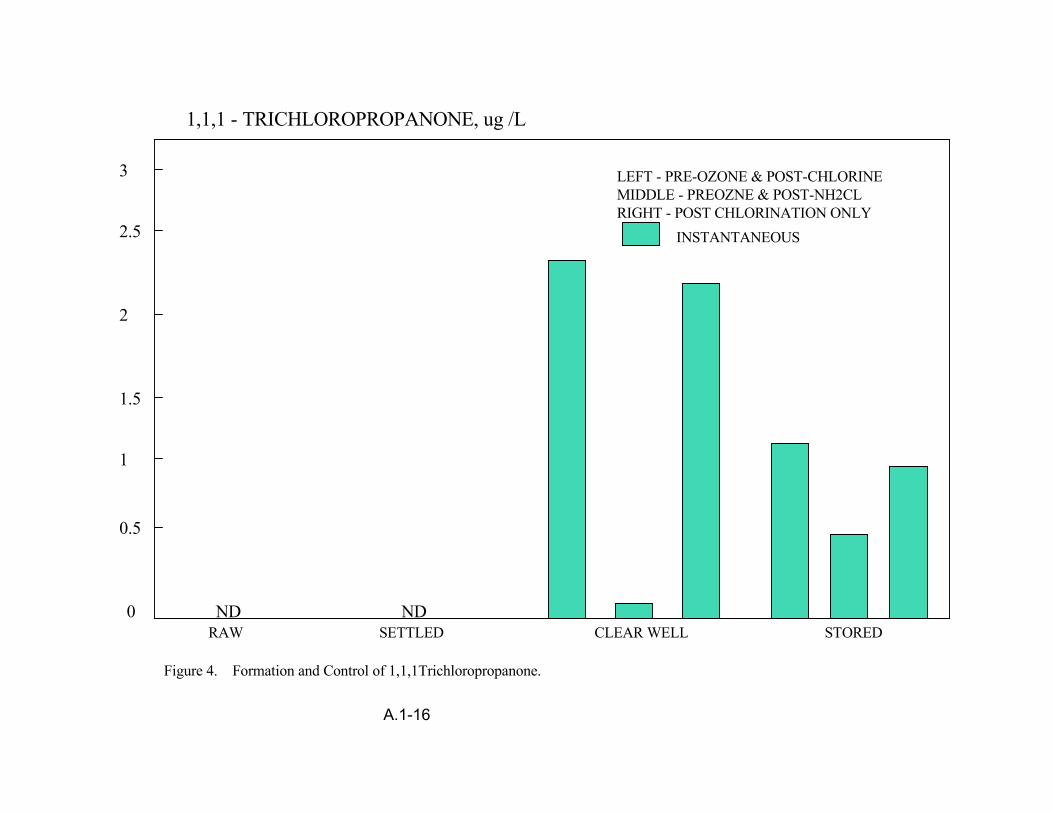
1,1,1 - TRICHLOROPROPANONE, ug /L
3
2.5
2
1.5
1
0.5
LEFT - PRE-OZONE & POST-CHLORINE MIDDLE - PREOZNE & POST-NH2CL RIGHT - POST CHLORINATION ONLY
INSTANTANEOUS
ND ND0RAW SETTLED CLEAR WELL STORED
Figure 4. Formation and Control of 1,1,1Trichloropropanone.
A.1-16
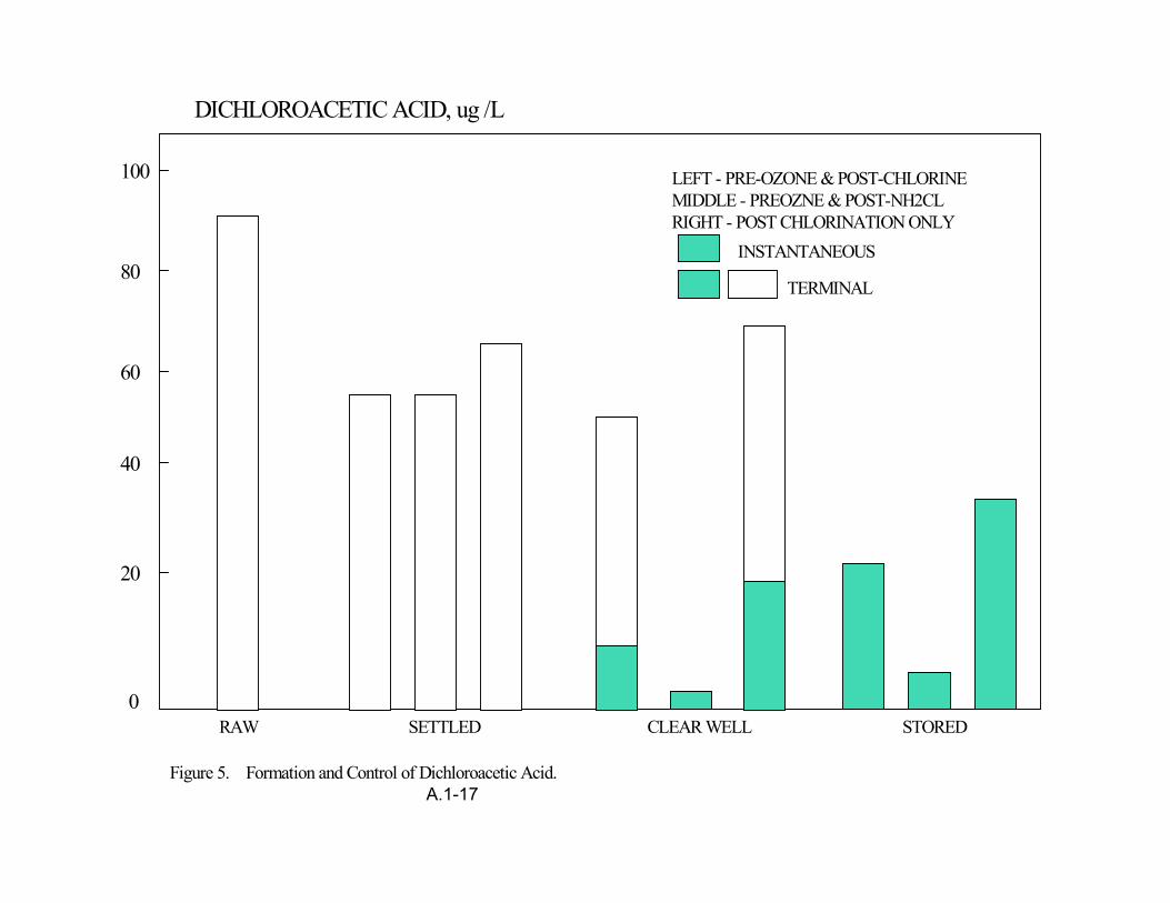
DICHLOROACETIC ACID, ug /L
100
80
60
40
20
LEFT - PRE-OZONE & POST-CHLORINE MIDDLE - PREOZNE & POST-NH2CL RIGHT - POST CHLORINATION ONLY
INSTANTANEOUS
TERMINAL
0RAW SETTLED CLEAR WELL STORED
Figure 5. Formation and Control of Dichloroacetic Acid. A.1-17
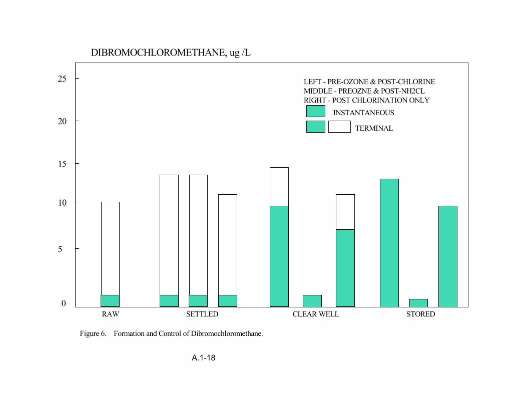
DIBROMOCHLOROMETHANE, ug /L
25
20
15
10
5
LEFT - PRE-OZONE & POST-CHLORINE MIDDLE - PREOZNE & POST-NH2CL RIGHT - POST CHLORINATION ONLY
INSTANTANEOUS
TERMINAL
0RAW SETTLED CLEAR WELL STORED
Figure 6. Formation and Control of Dibromochloromethane.
A.1-18
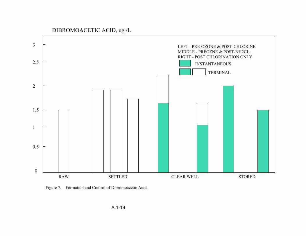
DIBROMOACETIC ACID, ug /L
3
2.5
2
1.5
1
0.5
0 RAW SETTLED CLEAR WELL STORED
LEFT - PRE-OZONE & POST-CHLORINE MIDDLE - PREOZNE & POST-NH2CL RIGHT - POST CHLORINATION ONLY
INSTANTANEOUS
TERMINAL
Figure 7. Formation and Control of Dibromoacetic Acid.
A.1-19
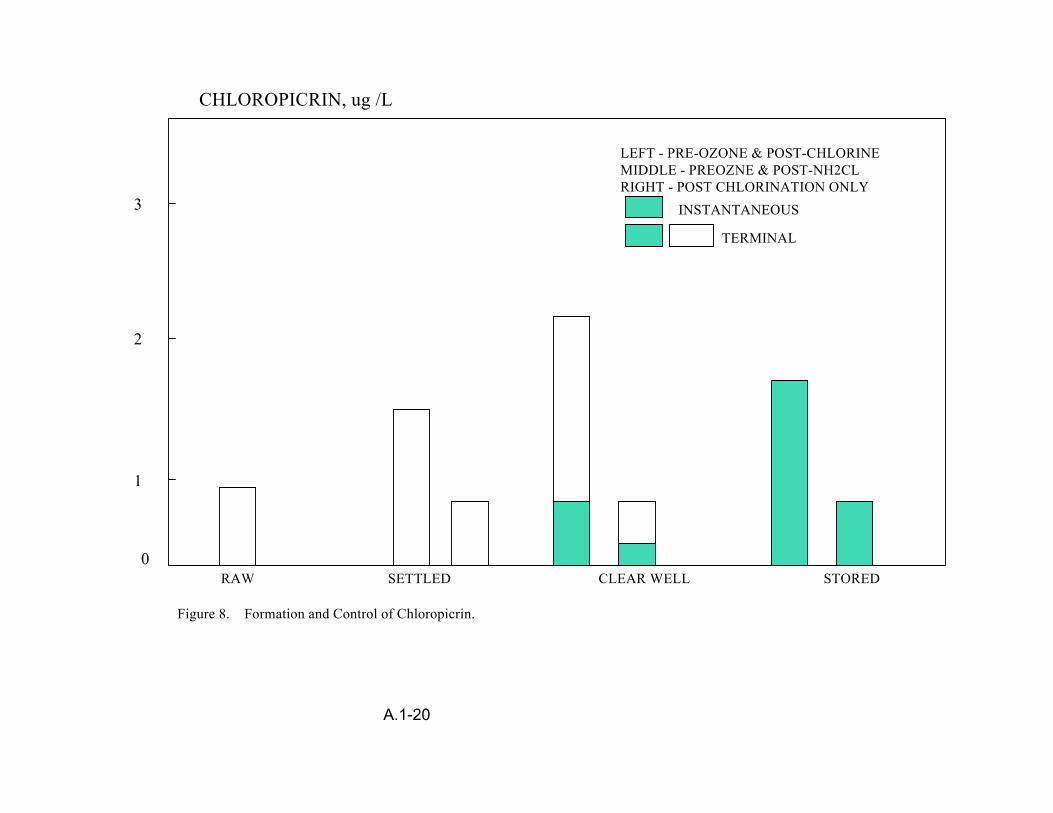
CHLOROPICRIN, ug /L
3
2
1
0 RAW SETTLED CLEAR WELL STORED
LEFT - PRE-OZONE & POST-CHLORINE MIDDLE - PREOZNE & POST-NH2CL RIGHT - POST CHLORINATION ONLY
INSTANTANEOUS
TERMINAL
Figure 8. Formation and Control of Chloropicrin.
A.1-20
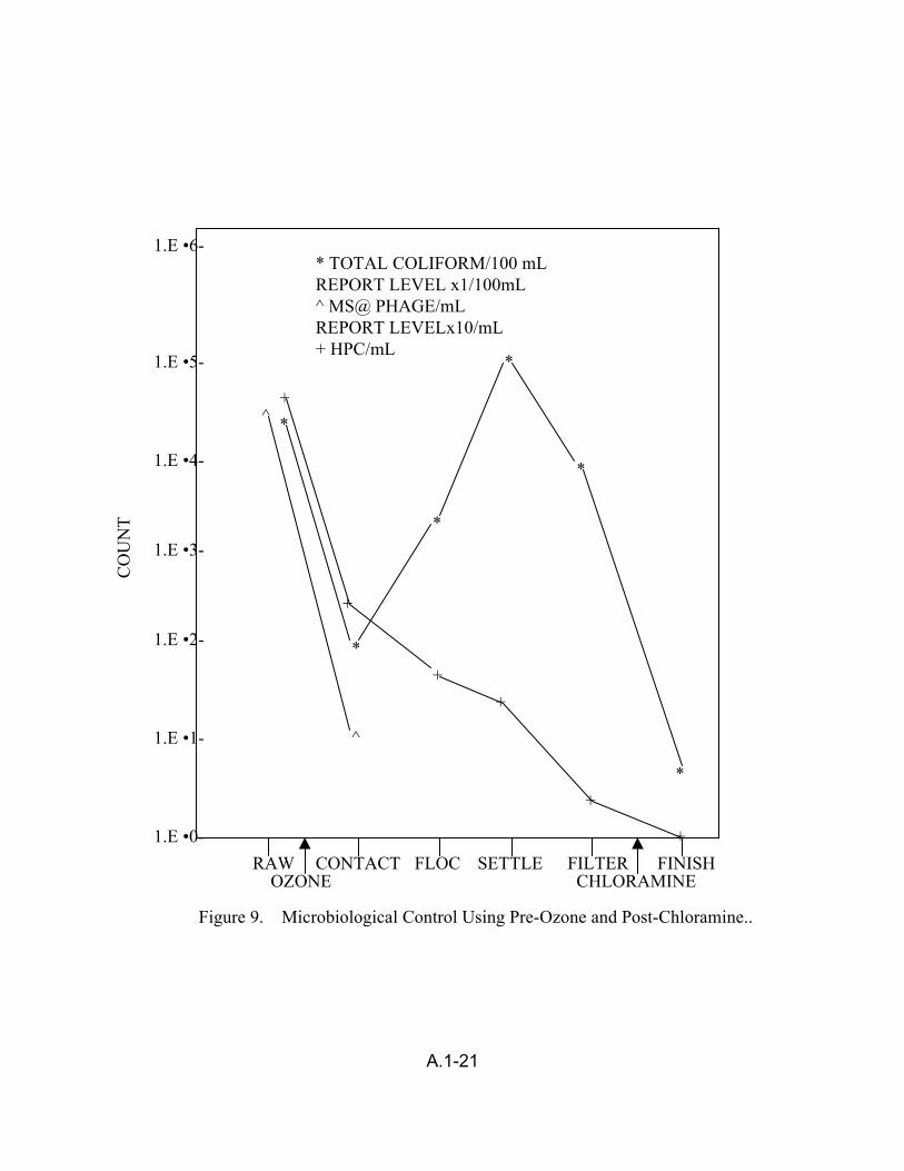
CO
UN
T
* TOTAL COLIFORM/100 mL REPORT LEVEL x1/100mL ^ MS@ PHAGE/mL REPORT LEVELx10/mL + HPC/mL
1.E •6-
1.E •4-
1.E •3-
1.E •2-
1.E •1-
1.E •0-
1.E •5-
^
^
RAW CONTACT FLOC SETTLE FILTER FINISH OZONE CHLORAMINE
+
+
+ +
+
+
*
*
*
*
*
*
Figure 9. Microbiological Control Using Pre-Ozone and Post-Chloramine..
A.1-21
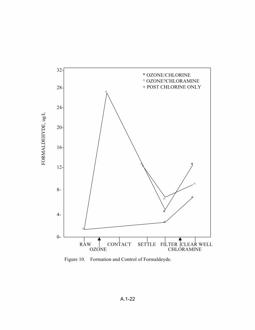
FOR
MA
LDEH
YD
E, u
g/L
32-
28-
24-
20-
16-
12-
8-
4-
0-
* OZONE/CHLORINE ^ OZONE?CHLORAMINE + POST CHLORINE ONLY
RAW CONTACT SETTLE FILTER CLEAR WELL OZONE CHLORAMINE
+
+ ^
^
^
^
^
*
*
Figure 10. Formation and Control of Formaldeyde.
A.1-22
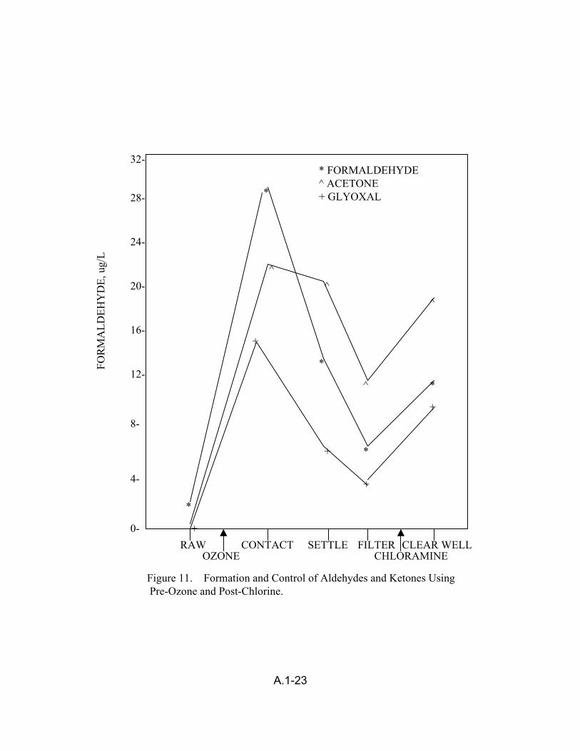
FOR
MA
LDEH
YD
E, u
g/L
32-
28-
24-
20-
16-
12-
8-
4-
0-
* FORMALDEHYDE ^ ACETONE + GLYOXAL
RAW CONTACT SETTLE FILTER CLEAR WELL OZONE CHLORAMINE
+
+
+
+
+
^
^
^ ^
*
*
*
*
*
Figure 11. Formation and Control of Aldehydes and Ketones Using Pre-Ozone and Post-Chlorine.
A.1-23
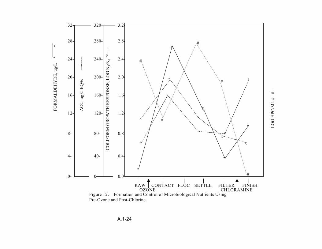
*
*FO
RM
ALD
EHY
DE,
ug/
L
32-
28-
24-
20-
16-
12-
8-
4-
0-
AO
C, u
g C
-EQ
/L +
+
320
280-
240-
200-
160-
120-
80-
40-
0
CO
LIFO
RM
GR
OW
TH R
ESPO
NSE
, LO
G N
5/N0
^ ^
3.2-
2.8-
2.4-
2.0-
1.6-
1.2-
0.8-
0.4-
0.0-*
*
*
*
*
+
+ +
+
+
#
#
#
#
#
^ ^
^
^
^
RAW OZONE
CONTACT FLOC SETTLE FCHLORAMINE ILTER FINISH
Figure 12. Formation and Control of Microbiological Nutrients Using Pre-Ozone and Post-Chlorine.
LOG
HPC
/ML
# #
A.1-24

APPENDIX B
Animal Bioassay and In Vitro Testing
APPENDIX B.1 DBP MIXTURE RISK ESTIMATION – ALTERNATIVE MODELS
The U.S. EPA published the Guidelines for the Health Risk Assessment of
Chemical Mixtures (U.S. EPA, 1986) in which three approaches to quantitation of health
risk for a chemical mixture are recommended, depending upon the type of available
data (Teuschler and Hertzberg, 1995). In the first approach, toxicity data on the mixture
of concern are available; the quantitative risk assessment is done directly from these
preferred data. In the second approach, when data are not available for the mixture of
concern, the Guidelines recommend using data on a “sufficiently similar” mixture.
Similarity is judged from data on component composition of the mixture, component
proportions within the mixture, source of emission, and health effects due to exposure to
these similar mixtures. If the mixture of concern and the similar mixture are judged to be
similar, then the quantitative risk assessment for the mixture of concern may be derived
from health effects data on the similar mixture. Finally, the third approach is to evaluate
the mixture through an analysis of its components, e.g., using dose-addition for
systemic effects and response-addition for estimates of cancer risk. These procedures
include a general assumption that interaction effects at low dose levels either do not
occur at all or are small enough to be insignificant to the risk estimate.
The Guidelines recommend the incorporation of interactions data when available,
if not as part of the quantitative process, then as a qualitative evaluation of the risk.
There are many terms used to describe interaction effects among chemicals, but the
two most common are synergism (the effect of the combination is greater than that
suggested by the component toxic effects under additivity) and antagonism (the effect of
the combination is less than that suggested by the component toxic effects under
B.1-1
additivity) (Hertzberg et al., in press). Interaction effects are more likely to occur at
higher dose levels where toxicologic processes are affected, e.g., competition for
receptor sites by a mixture of chemicals with a similar mechanism of action can result in
an antagonistic effect.
As stated above, dose-addition and response-addition are similar in that they are
both component based approaches that do not include interactions information because
they are generally applied to mixtures that occur together at low dose levels. Under
dose-addition, the first step is to scale the doses of the components for potency and add
the doses together; the mixtures risk is then estimated for the combined mixtures dose.
Under response-addition, the risks are first determined for the individual components;
the mixtures risk is then estimated by adding the individual risks together. These
processes are fundamentally different and require different assumptions of the data in
order for them to be used appropriately.
Dose-addition is different from response-addition because two assumptions are
made: that all of the components have similar uptake, pharmacokinetics and toxicologic
processes, and that the (log probit) dose-response curves of the components are
parallel (Teuschler and Hertzberg, 1995). This means that, for equal effects, the dose of
one component is a constant multiple of the dose of a second component. Usually the
assumption is made that the same constant multiple applies to any effect. Hertzberg et
al. (1999) note that dose-addition often does a reasonable job of predicting the toxicities
of mixtures composed of a variety of both similar and dissimilar compounds (Pozzani et
al., 1959; Smyth et al., 1969, 1970; Murphy, 1980; Ikeda, 1988; Feron et al., 1995),
although exceptions have been noted. Dose-addition is particularly useful in situations
B.1-2
where the dose for each individual component is at a level at which effects are not
expected to occur or be observable; when the doses are combined, effects are then
expected or observed in response to the higher dose level of the mixture. Often, dose-
addition is applied by scaling the potencies of all the components in the mixture to an
index chemical, adding the scaled doses together to give the equivalent dose in terms
of the index chemical, and using the index chemical’s dose-response curve to estimate
risk for the total mixture dose.
Response-addition is different from dose-addition in that it does not assume
similar kinetics or a similar mode of action and does not assume parallel dose-response
curves. It assumes that the components of the mixture are considered to be functionally
independent of one another at low exposure levels (Mumtaz and Hertzberg, 1993), so
that the risks may be added together. Because response-addition does not require a
similar mode of action across the chemicals in the mixture, it allows for combining risks
across different types of endpoints, unlike dose-addition. Response-addition is
particularly useful when the effect of concern is thought to be present at low dose levels
for each of the component chemicals, even though it is highly unlikely to be observable
at these low levels in either epidemiologic or toxicologic studies; the mixture risk is then
the sum of the individually low risks of the independently acting component chemicals.
For example, response-addition has often been used for the risk assessment of
mixtures of carcinogens (Gaylor et al., 1997; U.S. EPA, 1989).
The approach that is to be applied within the comparative risk decision analysis is
to work with component information, using appropriate additivity assumptions to
combine data on exposure levels for specific drinking water treatment scenarios with
B.1-3
dose-response estimates from animal data to generate human health risk estimates for
the mixtures of concern. The advantage of using the single chemical dose-response
toxicity data and combining them with treatment-specific exposure information is that
this method allows for relative comparisons of health risks across the treatments. In
addition, it allows for future health risk comparisons of any proposed decreases in the
allowable levels of DBPs in the finished drinking water. Any available interactions data
indicating that the mixture components may interact in a synergistic or antagonistic way
will be used only as qualitative information in the analysis.
Although estimates of human cancer, reproductive or development risks may be
taken from the epidemiologic literature, these data do not distinguish the risks across
various treatment scenarios. Most of the epidemiologic data simply distinguishes
between chlorinated or non-chlorinated water, or between chlorinated surface water and
groundwater without a detailed exposure characterization (Morris, 1992). Therefore,
dose-response estimates of health risks across treatments cannot be easily obtained.
Additional data from epidemiologic studies may be used from the perspective of
generating data used in establishing the human dose-response relationship, as a
guidepost indicating which biochemical mechanism to evaluate for potential interaction
with other chemicals, to corroborate estimates of human health risk calculated from the
animal data, or to provide upper bound risk estimates as part of the sensitivity analysis.
Human exposures are difficult to interpret, owing to exposure to a multitude of
chemicals daily. Some epidemiologic studies have been criticized for this, but those
studies still present data which may be useful, if only qualitative. Studies correlating
observed toxicity with exposure to agent(s), whether from laboratory animals or
B.1-4
humans, are of more value when specific components are identified. Some
investigations have been performed on human populations where the only identifier is
“disinfection with chlorine” versus “disinfection with chlorine dioxide”. While those data
are better than none at all, a more clearly defined exposure regimen would be
beneficial. This is rarely the case in more well controlled studies with laboratory
animals, where exact doses of DBP chemicals are known.
REFERENCES
Feron, V.J., J.P. Groten, D. Jonker, F.R. Cassess and P.J. van Bladeren. 1995. Toxicology of chemical mixtures: Challenges for today and the future. Toxicol. 105:415-427.
Gaylor, D.W., J.A. Axelrad, R.P. Brown et al. 1997. Health risk assessment practices in the U.S. Food and Drug Administration. Reg. Toxicol. Pharmacol. 26:307-321.
Hertzberg, R.C., G. Rice and L. Teuschler. 1999. Methods for health risk assessment of combustion mixtures. In: Hazardous Waste Incineration: Evaluating the Human Health and Environmental Risks, S. Roberts, C. Teaf, and J. Bean Ed. p. 105-148.
Ikeda, M. 1988. Multiple exposure to chemicals. Reg. Toxicol. Pharmacol. 8:414-421.
Morris, R.D., A.-M. Audet, I.F. Angelillo, T.C. Chalmers and F. Mosteller. 1992. Chlorination, chlorination by-products, and cancer: A meta-analysis. Am. J. Publ. Health. 82:955-963. (Erratum: Am J Public Health 1993;83:1257).
Mumtaz, M. and R.C. Hertzberg. 1993. The status of interactions data in risk assessment of chemical mixtures. In: Hazard Assessment of Chemicals, J. Saxena, Ed. Hemisphere Publishing Corporation, Washington, DC. 8:47-79.
Murphy, S.D. 1980. Assessment of the potential for toxic interactions among environmental pollutants. In: The Principles and Methods in Modern Toxicology, C.L. Galli, S.D. Murphy, and R. Paoletti, Ed. Elsevier/North Holland Biomedical Press, Amsterdam, The Netherlands.
B.1-5
Pozzani, U.C., C.S. Weil and C.P. Carpenter. 1959. The toxicological basis of threshold values: 5. The experimental inhalation of vapor mixtures by rats, with notes upon the relationship between single dose inhalation and single dose oral data. Am. Ind. Hyg. Assoc. J. 20:364-369.
Smyth, H.F., C.S. Weil, J.S. West and C.P. Carpenter. 1969. An exploration of joint toxic action: I. Twenty-seven industrial chemicals intubated in rats in all possible pairs. Toxicol. Appl. Pharmacol. 14:340-347.
Smyth, H.F., C.S. Weil, J.S. West and C.P. Carpenter. 1970. An exploration of joint toxic action. II. Equitoxic versus equivolume mixtures. Toxicol. Appl. Pharmacol. 17:498-503.
Teuschler, L.K. and R.C. Hertzberg. 1995. Current and future risk assessment guidelines, policy, and methods development for chemical mixtures. Toxicology. 105:137-144.
U.S. EPA. 1986. Guidelines for the Health Risk Assessment of Chemical Mixtures. Federal Register. 51(185):34014-34025.
U.S. EPA. 1989. Risk Assessment Guidance for Superfund, Vol. 1, Part A. EPA/540/1-89/002.
B.1-6
APPENDIX B.2 THE QUANTITATIVE STRUCTURE ACTIVITY RELATIONSHIP MODELING METHODOLOGY
B.2.1 BACKGROUND
The earliest version of TOPKAT® (Toxicity Prediction by Komputer-assisted
Technology) was introduced in 1987 by Health Designs, Inc. A complete redevelopment
of the earliest version led to the introduction of TOPKAT 3.0 in 1995. Subsequently,
TOPKAT 3.0 was enhanced to 5.0 in 1997 to include support for moiety analysis. These
software packages are designed for the accurate and rapid assessment of the toxicity of
chemicals solely from their molecular structure. Both software packages utilize robust,
cross-validated Quantitative Structure-Toxicity Relationship (QSTR) models for
assessing specific health- related endpoints, e.g. rodent oral carcinogenicity (NTP),
Ames mutagenicity, developmental toxicity potential, rat oral chronic Lowest-Observed-
Adverse-Effect Levels (LOAEL), rat oral LD50 , skin sensitization, fathead minnow LC50 ,
and Daphnia magna EC50. In addition, a Log P QSAR model is also available, where P
is the ratio of the solubility in octanol compared to the solubility in water and is known as
the octanol-water partition coefficient.
B.2.2 STRUCTURE-BASED MODELS
Structure-based toxicity assessment approaches can be classified into two types;
namely, Expert Systems (Human and Artificial) and QSTR approaches. Expert Systems
approaches are based on a collection of rules derived from existing subject knowledge
and stored in computer memory. QSTR-based model is a quantitative relationship
between numerical measure of toxicity and a set of structural descriptors. The
backbone of this approach is the effective quantification of salient structure attributes.
B.2-1

Such attributes include electronic (valence, sigma, pi and lone-pair), bulk (molecular
weight, size corrected E-values) and shape (molecular shape and symmetry) (Gombar,
1998). Such models are developed for predicting various endpoints (e.g.
carcinogenicity and developmental toxicity) and are based on very carefully selected
studies from the literature using extremely stringent criteria.
B.2.3 STRUCTURE-BASED MODEL DEVELOPMENT
In principle, a structure-based toxicity model is a quantitative relationship
between a numerical measure of toxicity and a set of structure descriptors, i.e.,
T = f (S),
where T is a measure of toxicity (e.g. LD50 , LOAEL, indicator of carcinogenicity ), S is a
set of numerical quantities representing different structural attributes, and f is a
mathematical function (HDI, 1995). These structure-toxicity relationships are generally
called quantitative structure-toxicity relationships (QSTR) models or equations, because
by knowing the function, f, and providing the values of S for any chemical one could
estimate its toxicity, T.
A special case in which (f) represents a linear multiple discriminant function is the
QSTR equation below which is a algebraic summation of all identified descriptors to
compute a probable value of toxicity for a submitted chemical structure. The form of a
QSTR is:
Computed Toxicity Value = Coeff1 × Var1 (Discriminant Score) + Coeff2 × Var2
+ Coeff3 × Var3 + ... + Coeffn × Varn + constant
B.2-2
The variables in the above QSTR equation are the calculated values of the
structure descriptors; the coefficients are the statistical weights associated with these
descriptors. During the development of the equation these weights are optimized. The
product of the descriptor variable and the coefficient is the descriptor’s contribution to
the estimated toxicity. If the contribution is positive it increases the probability of toxicity
whereas a decrease in probability is denoted by a negative value. The descriptors used
in TOPKAT 3.0/5.0 models quantify the electronic, shape and symmetry attributes of a
molecular structure. The electronic attributes are expressed in terms of the
electrotopological E-state values (Gombar, 1998) of specially designed 1-atom and
2-atom fragments of non-hydrogen atoms in different hybrid and hybridization states
called HDi substructures.
Toxicity values are computed by summing the contributions of the individual
descriptors. For assessing toxicity values such as the LOAEL and LC50, this sum is
transformed into a weight/weight unit (mg/kg) and weight/volume unit (mg/L). For
carcinogens, mutagens, and developmental toxicants, this sum is transformed into a
probability value between 0.0 and 1.0. For such 2-group classifications, a value
between 0.0 and 0.3 is considered negative or of low probability; a value between 0.3
and 0.7 is considered indeterminate (i.e., too near equal probability) for an assessment
to be meaningful and a value above 0.7 is considered to be positive.
B.2.4 MODEL VALIDATION
These models are based on both discriminant and regression analyses using
dichotomous and continuous scales, respectively. It is relatively easy to develop a
tentative QSTR with good correlation (r2); however, a good R2 does not necessarily
B.2-3
indicate that the model is appropriate for predictive purposes. Therefore, it is essential
to further validate these models based on a variety of diagnostics (Gombar et al., 1997).
These diagnostics include: (a) all descriptors in the function are significant, (b) no
compounds with unique variables are in the training set, (c) no influential or outlier
compounds remain in the training set, (d) residuals are normally distributed and (e)
cross validation performance (r2cv) is not significantly different from the performance (r2)
on the training set. Unless these characteristics are established in a QSTR, it cannot be
considered robust and, therefore, its statistical quality is questionable.
B.2.5 MODEL ACCURACY
In the case of the Developmental Toxicity Model (Gombar et al., 1995) stringent
criteria was applied to 5559 open literature citations containing experimental data on
developmental toxicity with the selection of 1238 rat studies for the development of the
model. However, 830 of these bioassays were not usable due to inherent problems in
protocols and 34 bioassays were deleted due to uncertain structure, organometallics
and mixtures. Ultimately, the compounds suitable for QSTR models were reduced from
374 to 273 based on the fact that some studies were performed at only one dose only
and both DT and MT were observed at that dose, and for some studies, neither DT nor
MTD was reported even at the highest dose. Based on specific criteria a DTP score
between 1 and 4 was assigned to each of the 273 chemicals. Ultimately, 273 chemicals
were used in the development of three developmental toxicity submodels (aliphatic,
carboaromatic and heteroaromatic). The cross-validation (leave-one-out) accuracy of
the three submodels range from 86.1% to 88.6% in terms of sensitivity (known
developmental toxicants identified as positive) and 86% to 97.4% in terms of specificity
B.2-4
(known non-developmental toxicants identified as negative). The indeterminants ranged
from 2.2 to 2.5%. Each submodel is comprised of about the same number of
compounds to give a total of 273 compounds.
The NTP Rodent Carcinogenicity Model comprises four statistically significant
and cross-validated QSTR models, and the data from which these models were derived.
Each QSTR model relates to a specific sex/species combination: female rat, male rat,
and female mouse, male mouse. The basis for each model are the 366 rodent
carcinogenicity studies conducted by the National Cancer Institute (NCI) and the
National Toxicology Program (NTP) utilizing inbred rats and hybrid mice. In selecting
the most appropriate studies, stringent criteria was uniformly applied to all NCI/NTP
studies and any studies not conforming to the predefined standards of purity, exposure
duration, route of exposure, dose levels, etc., were not included in the training sets for
developing QSTR models for carcinogenicity. For instance, results from 158
carcinogenicity assays in the female rat could not be included in the training set for
various reasons (Gombar et al., 1997). With respect to the accuracies of these four
carcinogenicity submodels, the sensitivity (% of known carcinogens predicted as
carcinogens) ranged from 82% in the case of the male rat to 91% in the case of the
female rat. Prediction of non carcinogens as non carcinogens (specificity) ranged from
82% in the case of the male rat to 94% for the male mouse. Percent indeterminants
were 11, 1, 1 and 5 for the male rat, female rat, male mouse and female mouse,
respectively. There were approximately equal number of compounds in each submodel
to give a total of 815 compounds.
B.2-5

B.2.6 QUALITY ASSURANCE/CONTROL
An established data base was used to develop the QSTR models for predicting
the various health-related endpoints of novel structures have been accumulated,
evaluated and standardized the software developer. These data include, but are not
limited to, chemical structure depictions, Chemical Abstract Service (CAS) Registry
numbers, experimental toxicity values, and reference citations. All of the models in the
software package have been developed by qualified statisticians, toxicologists,
computational chemists, and computer programmers, specializing in QSTR.
B.2.7 QSTR ANALYSES
B.2.7.1 Developing the Hypothesis (Prediction) via Univariate and Multivariate Analyses
In general, QSTR models are limited in their applicability, since they are derived
from experimentally measured toxicity values involving a limited number of descriptors.
Consequently, it is important to determine whether the structural attributes (descriptors)
of the query compound are represented in the compounds used for model development.
In order to assess whether the estimated toxicity is meaningful or not, and to assure
reproducibility of all the results, this software program has incorporated algorithms that
have been thoroughly tested. These algorithms (Gombar, 1998; HDI, 1995) are termed
univariate (Coverage Examination) and multivariate [Optimum Prediction Space
Examination (OPS)] analyses.
The univariate analysis determines whether all of the structural fragments of the
query structure are well-represented in the model data base or training set and the
multivariate analysis determines whether the query structure fits within or near the
B.2-6

periphery of the OPS of the equation. The OPS of a QSTR is a multi-dimensional
space, the number of dimensions being one more than the number of model descriptors
of the QSTR. An important characteristic of the OPS is that within and near its periphery
(permissible limits) the QSTR may be applied with confidence. If either of these criteria
(univariate and multivariate analyses) are not satisfied, a warning is displayed; however,
if they are satisfied “All Validation Criteria Satisfied” is displayed.
B.2.7.2 Testing the Hypothesis via Similarity Search
Using “Similarity Search” (HDI, 1995) this hypothesis can be tested against
compounds in the data base based on their QSTR similarity to the query structure.
TOPKAT displays the actual experimental and predicted results, whether the compound
was used in the training set, and the similarity distance (normalized to the query
compound) from the query on a scale of 0.0 to 1.0. The smaller the distance, the greater
the similarity. Acceptable results are obtained if one finds that the experimental and
predicted values of the “similarity search” compounds are in agreement and the
normalized similarity distance is 0.35 or less for discriminant analysis and less than 0.2
for regression analysis. If the experimental and predicted values do not agree then the
“similarity search” is considered unacceptable.
B.2-7

APPENDIX B.3 QSAR RESULTS FOR DBPs
A total of 253 compounds, identified as disinfection by-products (DBPs) by the
Office of Water, were analyzed for carcinogenicity and developmental toxicity using
TOPKAT®/QSTR software. All submitted query structures for either endpoint were
automatically subjected to univariate (Coverage) and multivariate (Optimum Prediction
Space) analyses, and ultimately generated a “hypothesis” in terms of probability.
Subsequently, the confidence in the hypotheses were tested by application of the
“similarity search” algorithm. The application of such diagnostic tools within the software
ensures the accuracy for each model prediction in terms of false-positives and false-
negatives.
The initial agreement between NCEA-Cin and the Office of Water (OW) was to
subject the 252 DBPs submitted by OW to QSTR analyses using TOPKAT software. In
view of the time constraints it was agreed upon that such prioritization of DBPs would
not include any rationalization as to why certain classes of chemicals based on
functional groups are active and others inactive. In general, there are two reasons for
prioritization; namely, regulatory decision making and research needs. This effort
focuses principally on the research needs for Stage 2 DBPS Rule for which there is little
health data available. Such data will assist OW in selecting high priority DBPs or
classes of DBPs for additional health effects studies and eliminating others.
The results of the 253 DBPs analyzed were tabulated (Table B.3-1) and
prediction patterns were observed within and between classes based on their functional
groups (e.g. alcohols, acids, etc.) and specific health related endpoints. A visual
representation of the QSAR analyses for the principal functional groups are presented
B.3-1
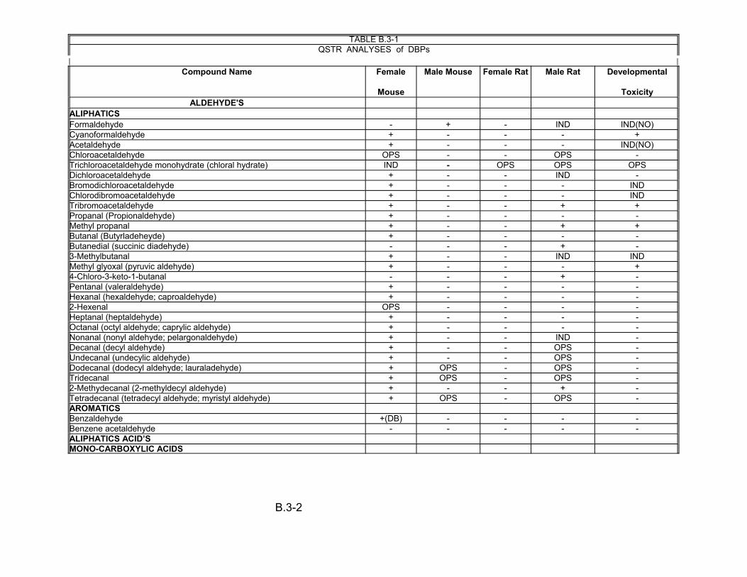
TABLE B.3-1 QSTR ANALYSES DBPs of
2 2Compound Name Female
Mouse
Male Mouse Female Rat Male Rat Developmental
Toxicity ALDEHYDE'S
ALIPHATICS Formaldehyde - + - IND IND(NO) Cyanoformaldehyde + - - - + Acetaldehyde + - - - IND(NO) Chloroacetaldehyde OPS - - OPS -Trichloroacetaldehyde monohydrate (chloral hydrate) IND - OPS OPS OPS Dichloroacetaldehyde + - - IND -Bromodichloroacetaldehyde + - - - IND Chlorodibromoacetaldehyde + - - - IND Tribromoacetaldehyde + - - + + Propanal (Propionaldehyde) + - - - -Methyl propanal + - - + + Butanal (Butyrladeheyde) + - - - -Butanedial (succinic diadehyde) - - - + -3-Methylbutanal + - - IND IND Methyl glyoxal (pyruvic aldehyde) + - - - + 4-Chloro-3-keto-1-butanal - - - + -Pentanal (valeraldehyde) + - - - -Hexanal (hexaldehyde; caproaldehyde) + - - - -2-Hexenal OPS - - - -Heptanal (heptaldehyde) + - - - -Octanal (octyl aldehyde; caprylic aldehyde) + - - - -Nonanal (nonyl aldehyde; pelargonaldehyde) + - - IND -Decanal (decyl aldehyde) + - - OPS -Undecanal (undecylic aldehyde) + - - OPS -Dodecanal (dodecyl aldehyde; lauraladehyde) + OPS - OPS -Tridecanal + OPS - OPS -2-Methydecanal (2-methyldecyl aldehyde) + - - + -Tetradecanal (tetradecyl aldehyde; myristyl aldehyde) + OPS - OPS -AROMATICS Benzaldehyde +(DB) - - - -Benzene acetaldehyde - - - - -ALIPHATICS ACID’S MONO-CARBOXYLIC ACIDS
B.3-2
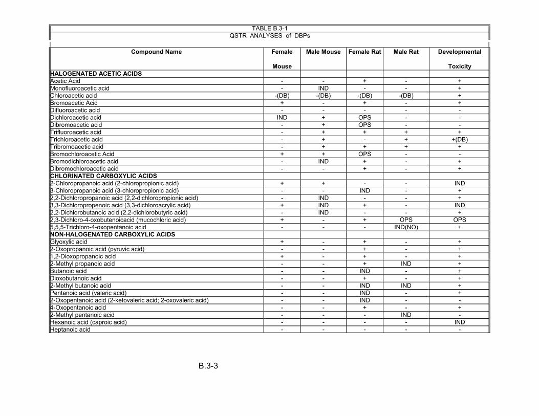
TABLE B.3-1 QSTR ANALYSES DBPs of
2 2Compound Name Female
Mouse
Male Mouse Female Rat Male Rat Developmental
Toxicity HALOGENATED ACETIC ACIDS Acetic Acid - + - + Monofluoroacetic acid - IND - - + Chloroacetic acid -(DB) -(DB) -(DB) -(DB) + Bromoacetic Acid + - + - + Difluoroacetic acid - - - - -Dichloroacetic acid IND + OPS - -Dibromoacetic acid - + OPS - -Trifluoroacetic acid - + + + + Trichloroacetic acid - + - + +(DB) Tribromoacetic acid - + + + + Bromochloroacetic Acid + + OPS - -Bromodichloroacetic acid - IND + - + Dibromochloroacetic acid - - + - + CHLORINATED CARBOXYLIC ACIDS 2-Chloropropanoic acid (2-chloropropionic acid) + + - - IND 3-Chloropropanoic acid (3-chloropropionic acid) - - IND - + 2,2-Dichloropropanoic acid (2,2-dichloropropionic acid) - IND - - + 3,3-Dichloropropenoic acid (3,3-dichloroacrylic acid) + IND + - IND 2,2-Dichlorobutanoic acid (2,2-dichlorobutyric acid) - IND - - + 2,3-Dichloro-4-oxobutenoicacid (mucochloric acid) + - + OPS OPS 5,5,5-Trichloro-4-oxopentanoic acid - - - IND(NO) + NON-HALOGENATED CARBOXYLIC ACIDS Glyoxylic acid + - + - + 2-Oxopropanoic acid (pyruvic acid) - - + - + 1,2-Dioxopropanoic acid + - + - + 2-Methyl propanoic acid - - + IND + Butanoic acid - - IND - + Dioxobutanoic acid - - + - + 2-Methyl butanoic acid - - IND IND + Pentanoic acid (valeric acid) - - IND - + 2-Oxopentanoic acid (2-ketovaleric acid; 2-oxovaleric acid) - - IND - -4-Oxopentanoic acid - - + - + 2-Methyl pentanoic acid - - - IND -Hexanoic acid (caproic acid) - - - - IND Heptanoic acid - - - - -
-
B.3-3
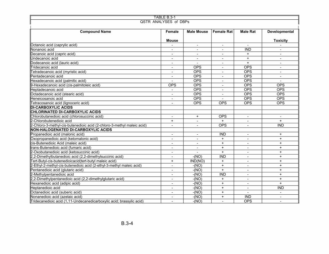
TABLE B.3-1 QSTR ANALYSES DBPs of
2 2Compound Name Female
Mouse
Male Mouse Female Rat Male Rat Developmental
Toxicity Octanoic acid (caprylic acid) - - - - -Nonanoic acid - - - IND -Decanoic acid (capric acid) - - - + -Undecanoic acid - - - + -Dodecanoic acid (lauric acid) - - - + -Tridecanoic acid - OPS - OPS -Tetradecanoic acid (myristic acid) - OPS - OPS -Pentadecanoic acid - OPS - OPS -Hexadecanoic acid (palmitic acid) - OPS - OPS -9-Hexadecanoic acid (cis-palmitoleic acid) OPS OPS - OPS OPS Heptadecanoic acid - OPS - OPS OPS Octadecanoic acid (stearic acid) - OPS - OPS OPS Heneicosanoic acid - OPS - OPS OPS Tetracosanoic acid (lignoceric acid) - OPS OPS OPS OPS DI-CARBOXYLIC ACIDS CHLORINATED DI-CARBOXYLIC ACIDS Chlorobutanedioic acid (chlorosuccinic acid) - + OPS - -2-Chlorobutenedioic acid + - + - + 2-Chloro-3-methyl-cis-butenedioic acid (2-chloro-3-methyl maleic acid) - - OPS - IND NON-HALOGENATED DI-CARBOXYLIC ACIDS Propanedioic acid (malonic acid) - - IND - + Oxopropanedioic acid (ketomalonic acid) - - + - + cis-Butenedioic Acid (maleic acid) - - + - + trans-Butenedioic acid (fumaric acid) - - + - + 2-Oxobutanedioic acid (ketosuccinic acid) - - + - + 2,2-Dimethylbutanedioic acid (2,2-dimethylsuccinic acid) - -(NO) IND - + Tert-Butyl-cis-butenedioicacid(tert-butyl maleic acid) + IND(NO) + - + 2-Ethyl-2-methyl-cis-butenedioic acid (2-ethyl-3-methyl maleic acid) - -(NO) + - + Pentanedioic acid (glutaric acid) - -(NO) + - + 2-Methylpentanedioic acid - -(NO) IND - + 2,2-Dimethylpentanedioic acid (2,2-dimethylglutaric acid) - -(NO) + - + Hexanedioic acid (adipic acid) - -(NO) + - + Heptanedioic acid - -(NO) + - IND Octanedioic acid (suberic acid) - -(NO) + - -Nonanedioic acid (azelaic acid) - -(NO) + IND -Tridecanedioic acid (1,11-Undecanedicarboxylic acid; brassylic acid) - -(NO) - OPS -
B.3-4

TABLE B.3-1 QSTR ANALYSES DBPs of
2 2Compound Name Female
Mouse
Male Mouse Female Rat Male Rat Developmental
Toxicity AROMATICS Benzoic Acid - - + - -3-Hydroxybenzoic acid - - - - -3,4-Dihydroxybenzoic acid (protochatechuic acid) - - + - -3-Methylbenzoic acid - - + - -4-Methylbenzoic acid - - + - -1,2-Benzene dicarboxylic acid - - IND - -1,3-Benzene dicarboxylic acid - - + - -1,4-Benzene dicarboxylic acid - - + - -1,2,3-Benzene tricarboxylic acid - OPS OPS - -1,2,4-Benzene tricarboxylic acid - OPS OPS - -1,3,5-Benzene tricarboxylic acid IND OPS OPS - -Phenylacetic acid - - + - +
KETONE'S ALIPHATICS
HALOGENATED KETONES Dichloroacetone - - OPS - -1,1-Dibromoacetone (1,1-Dibromopropanone) - + OPS - -1-Chlorodimethylglyoxal - - - - + Chloropropanone (chloroacetone) - - - - +(NO) 1,1-Dichloropropanone - - OPS - -1,3-Dichloropropanone - + - - + 1,1,1-Trichloropropanone - + - - + 1,1,3-Trichloropropanone (1,1,3-trichloroacetone) - + OPS - -1,1,1,3-Tetrachloropropanone - + OPS + + 1,1,3,3-Tetrachloropropanone OPS OPS OPS + OPS 1,1,1,3,3-Pentachloropropanone OPS + OPS IND -Hexachloropropanone - + - + + 1,1-Bromochloropropanone + + OPS - -1-Bromo-1,1-dichloropropanone - - - - + 1,1-Dichloro-2-butanone - - OPS - -3,3-Dichloro-2-butanone - - - - + 1,1,1-Trichloro-2-butanone - + - IND + 2,2-Dichloro-3-pentanone - - - - + NON-HALOGENATED KETONES
Acetone - - + + -
B.3-5

TABLE B.3-1 QSTR ANALYSES DBPs of
2 2Compound Name Female
Mouse
Male Mouse Female Rat Male Rat Developmental
Toxicity Glyoxal + - + Dimethylglyoxal (2,2-butanedione; diacetyl) - - - IND + Butanone - - +(NO) 3-Methyl-2-pentanone (sec-butyl methyl ketone) - - - + + Methyl isobutyl ketone - - - + + 3-Hexanone - - -3-Methyl-2,4-hexanedione - - - OPS OPS 2,6-Dimethyl-2,5-heptadiene-4-one OPS OPS OPS OPS -6-Methyl-5-hepten-3-one OPS OPS OPS - -6, 10-Dimethyl-5,9-undecadiene-2-one (Nerylacetone/Geranylacetone) OPS OPS OPS OPS OPS
CYCLIC KETONES 2,2,4-Trichloro-1,3-cyclopentenedione + - - - -2-Chlorocyclohexanone - OPS - - -3-Methyl-1,2,4-cyclopentanetrione - - - - OPS 2,5-Dimethylcyclopentanone - - - - OPS 2,3,4-Trimethylcyclopent-2-en-1-one - - - - OPS 2,6,6-Trimethyl-2-cyclohexene-1,4-dione - - - IND OPS 1,3,3-Trimethyl-1-7-oxabicyclo-[4.1.0]-heptane-2,5-dione - - - IND -AROMATICS 1-[4-(1-Hydroxy-1-methylethyl) phenyl]-ethanone - - - - -1-[4-(1-Methylethyl) phenyl]-ethanone - + - + -1,1-(1,4-Phenylene) bis-ethanone - + - + -2,6-Tert-butyl-1,4-Benzoquinone + - - IND -
LACTONE'S Dihydro-4,5-dichloro-2-(3H)-furanone - - - - OPS 5-Hydroxy-5-trichloromethyl-2-furanone + + - IND IND 3-Chloro-4 (dichloromethyl)-2-(5H)-furanone (red-MX) - - OPS - OPS 3-Chloro-4-dichloromethyl-5-hydroxy-2-(5H)-furanone (MX) - IND OPS - -3-Chloro-4-(bromochloromethyl)-5-hydroxy-2(5H)-furanone (BMX-1) + OPS OPS - -3-Chloro-4-(dibromomethyl)-5-hydroxy-2(5H)-furanone(BMX- 2) - + OPS - -3-Bromo-4-(dibromomethyl)-5-hydroxy-2(5H)-furanone (BMX-3) - + OPS - -2-Chloro-3-(dichloromethyl)-butenoic acid (ox-MX) - + OPS - -(E)-2-Chloro-3-(dichloromethyl)-4-oxobutenoic acid (EMX) + - OPS - -(E)-2-Chloro-3-(dichloromethyl) butenedioic acid (ox-EMX) - + OPS - -5-Methyl-2-furancarboxylic acid - + + - -4-Dodecyl-5-ethyl-2(5H)furanone - OPS - OPS OPS
- +
- -
- -
B.3-6
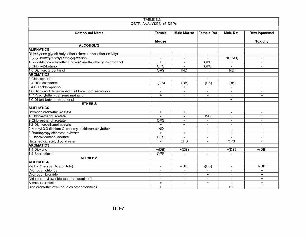
TABLE B.3-1 QSTR ANALYSES DBPs of
2 2Compound Name Female
Mouse
Male Mouse Female Rat Male Rat Developmental
Toxicity ALCOHOL'S
ALIPHATICS Di (ethylene glycol) butyl ether (check under ether activity) - - - - -2-[2-(2-Butoxyethoxy) ethoxyl]-ethanol - - - IND(NO) -1-[2-(2-Methoxy-1-methylethoxy)-1-methylethoxyl]-2-propanol + - OPS + -3-Chloro-2-butanol OPS - OPS - -4,5-Dichloro-2-pentanol OPS IND - IND -AROMATICS 2-Chlorophenol - - - - -2,4-Dichlorophenol -(DB) -(DB) -(DB) -(DB) -2,4,6-Trichlorophenol - + - - -4,6-Dichloro-1,3-benzenediol (4,6-dichlororesorcinol) - - - - -4-(1-Methylethyl)-benzene methanol + - + - +2,6-Di-tert-butyl-4-nitrophenol - - - + -
ETHER'SALIPHATICSBromochloromethyl Acetate + + + - -1-Chloroethanol acetate - - IND + +2-Chloroethanol acetate OPS - - - -1,2-Dichloroethanol acetate + + - - -2-Methyl-3,3-dichloro-2-propenyl dichloromethylether IND - + - -3-Bromopropylchloromethylether + + + + +3-Chloro2-butanol acetate OPS - - - -Hexanedioic acid, dioctyl ester - OPS - OPS -AROMATICS1,4-Dioxane +(DB) +(DB) - +(DB) +(DB)1,4-Benzodioxin OPS - - - -
NITRILE'SALIPHATICSMethyl Cyanide (Acetonitrile) - -(DB) -(DB) - +(DB)Cyanogen chloride - - - - +Cyanogen bromide - - + - +Chloromethyl cyanide (chloroacetonitrile) - - - - +Bromoacetonitrile + - + - +Dichloromethyl cyanide (dichloroacetonitrile) + - - IND +
B.3-7
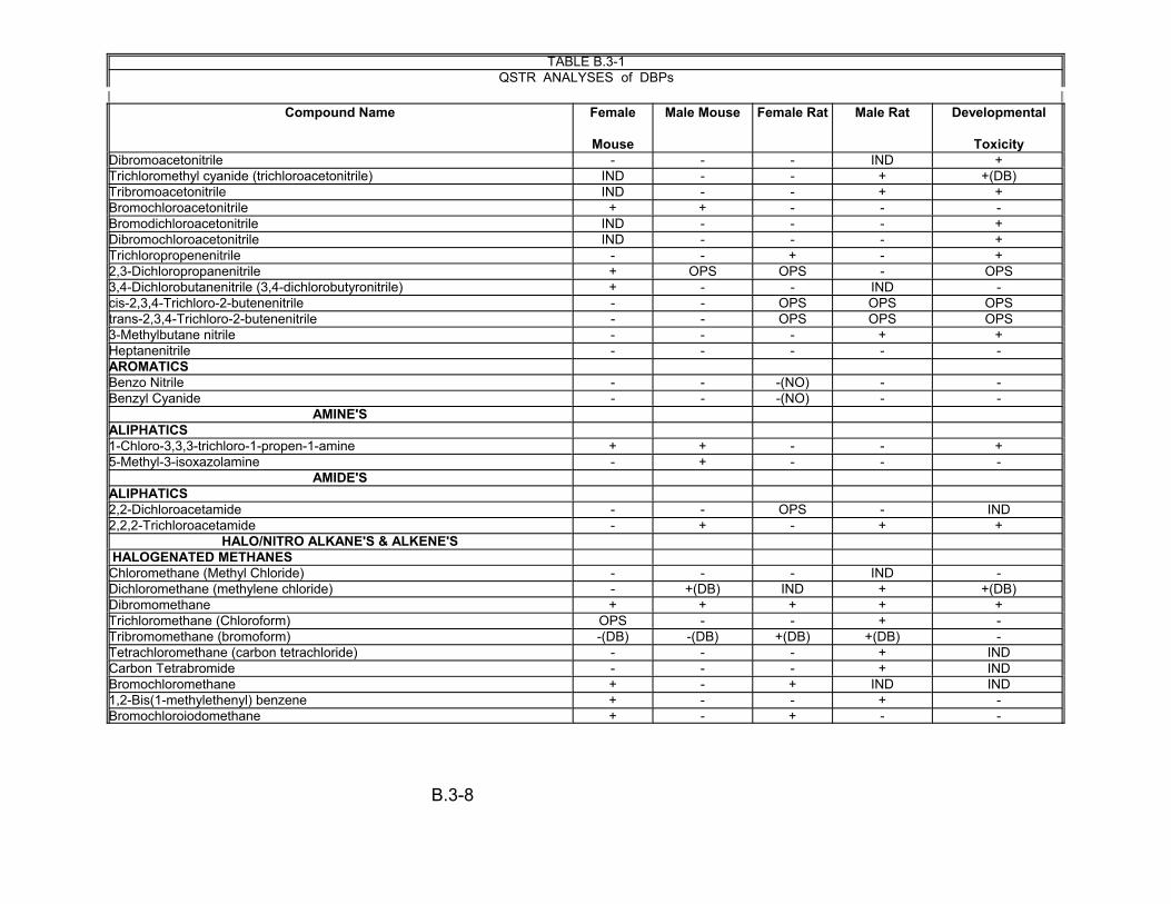
TABLE B.3-1 QSTR ANALYSES DBPs of
2 2Compound Name Female
Mouse
Male Mouse Female Rat Male Rat Developmental
Toxicity Dibromoacetonitrile - - - IND + Trichloromethyl cyanide (trichloroacetonitrile) IND - - + +(DB) Tribromoacetonitrile IND - - + + Bromochloroacetonitrile + + - - -Bromodichloroacetonitrile IND - - - + Dibromochloroacetonitrile IND - - - + Trichloropropenenitrile - - + - + 2,3-Dichloropropanenitrile + OPS OPS - OPS 3,4-Dichlorobutanenitrile (3,4-dichlorobutyronitrile) + - - IND -cis-2,3,4-Trichloro-2-butenenitrile - - OPS OPS OPS trans-2,3,4-Trichloro-2-butenenitrile - - OPS OPS OPS 3-Methylbutane nitrile - - - + + Heptanenitrile - - - - -AROMATICS Benzo Nitrile - - -(NO) - -Benzyl Cyanide - - -(NO) - -
AMINE'S ALIPHATICS 1-Chloro-3,3,3-trichloro-1-propen-1-amine + + - - + 5-Methyl-3-isoxazolamine - + - - -
AMIDE'S ALIPHATICS 2,2-Dichloroacetamide - - OPS - IND 2,2,2-Trichloroacetamide - + - + +
HALO/NITRO ALKANE'S & ALKENE'S HALOGENATED METHANES
Chloromethane (Methyl Chloride) - - - IND -Dichloromethane (methylene chloride) - +(DB) IND + +(DB) Dibromomethane + + + + + Trichloromethane (Chloroform) OPS - - + -Tribromomethane (bromoform) -(DB) -(DB) +(DB) +(DB) -Tetrachloromethane (carbon tetrachloride) - - - + IND Carbon Tetrabromide - - - + IND Bromochloromethane + - + IND IND 1,2-Bis(1-methylethenyl) benzene + - - + -Bromochloroiodomethane + - + - -
B.3-8
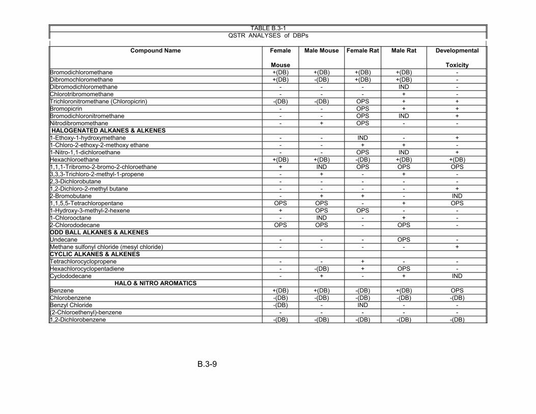
TABLE B.3-1 QSTR ANALYSES DBPs of
2 2Compound Name Female
Mouse
Male Mouse Female Rat Male Rat Developmental
Toxicity Bromodichloromethane +(DB) +(DB) +(DB) +(DB) -Dibromochloromethane +(DB) -(DB) +(DB) +(DB) -Dibromodichloromethane - - - IND -Chlorotribromomethane - - - + -Trichloronitromethane (Chloropicrin) -(DB) -(DB) OPS + + Bromopicrin - OPS + + Bromodichloronitromethane - - OPS IND + Nitrodibromomethane - + OPS - -HALOGENATED ALKANES & ALKENES
1-Ethoxy-1-hydroxymethane - - IND - + 1-Chloro-2-ethoxy-2-methoxy ethane - - + + -1-Nitro-1,1-dichloroethane - - OPS IND + Hexachloroethane +(DB) +(DB) -(DB) +(DB) +(DB) 1,1,1-Tribromo-2-bromo-2-chloroethane + IND OPS OPS OPS 3,3,3-Trichloro-2-methyl-1-propene - + - + -2,3-Dichlorobutane - - - - -1,2-Dichloro-2-methyl butane - - - - + 2-Bromobutane - + + - IND 1,1,5,5-Tetrachloropentane OPS OPS - + OPS 1-Hydroxy-3-methyl-2-hexene + OPS OPS - -1-Chlorooctane - IND - + -2-Chlorododecane OPS OPS - OPS -ODD BALL ALKANES & ALKENES Undecane - - OPS -Methane sulfonyl chloride (mesyl chloride) - - - - + CYCLIC ALKANES & ALKENES Tetrachlorocyclopropene - - + - -Hexachlorocyclopentadiene - -(DB) + OPS -Cyclododecane - + - + IND
HALO & NITRO AROMATICS Benzene +(DB) +(DB) -(DB) +(DB) OPS Chlorobenzene -(DB) -(DB) -(DB) -(DB) -(DB) Benzyl Chloride -(DB) - IND - -(2-Chloroethenyl)-benzene - - - - -1,2-Dichlorobenzene -(DB) -(DB) -(DB) -(DB) -(DB)
-
-
B.3-9
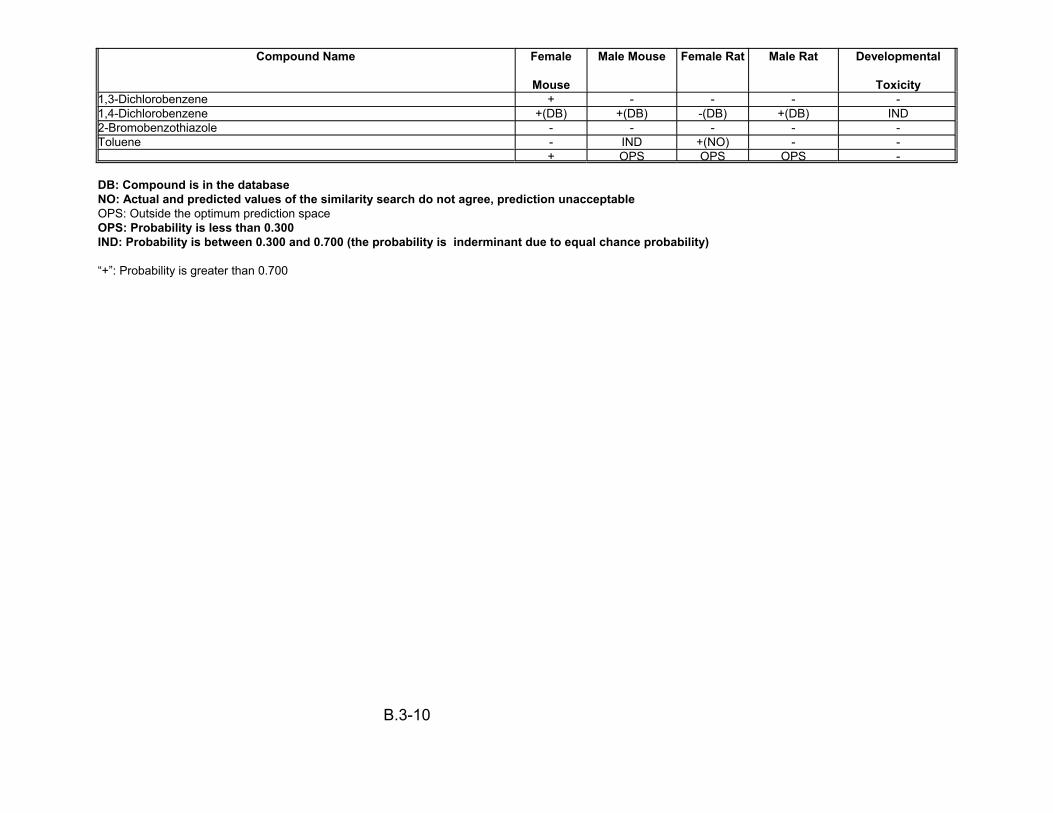
Compound Name Female
Mouse
Male Mouse Female Rat Male Rat Developmental
Toxicity 1,3-Dichlorobenzene + - - - -1,4-Dichlorobenzene +(DB) +(DB) -(DB) +(DB) IND 2-Bromobenzothiazole - - - - -Toluene - IND +(NO) - -
+ OPS OPS OPS -
DB: Compound is in the databaseNO: Actual and predicted values of the similarity search do not agree, prediction unacceptableOPS: Outside the optimum prediction space OPS: Probability is less than 0.300IND: Probability is between 0.300 and 0.700 (the probability is inderminant due to equal chance probability)
“+”: Probability is greater than 0.700
B.3-10

as bar graphs. An examination of the results obtained should aid in the prioritization of
these health-related endpoints for performing additional bioassay studies.
B.3.1 ALDEHYDES
Carcinogenicity
The carcinogenicity of aliphatic aldehydes is predicted to be gender specific in
that the majority aliphatic aldehydes (22/28) were predicted as carcinogens in the
female mouse and noncarcinogens in the male mouse. All aliphatic aldehydes were
predicted as noncarcinogens in female rats with a mixture of carcinogens/
noncarcinogens (5/28) in male rats. The two aromatic aldehydes, benzaldehyde and
benzacetaldehyde are predicted as noncarcinogens in all submodels with the exception
of the female mouse which predicts benzaldehyde to be carcinogenic.
Developmental Toxicity
With the exceptions of cyanoformaldehyde, tribromoacetaldehyde, methyl
propanal and methyl glyoxal, all other aliphatic and aromatic aldehydes (20/30) are
predicted negative for developmental toxicity.
Mono Carboxylic Acids
Halogenated Acetic Acids
Carcinogenicity
All monohalogenated acetic acids are predicted as noncarcinogens for both
female and male rats and mice with the exception of bromoacetic acid which is
predicted as a carcinogen in female rats and mice. Dihalogenated acetic acids are
predicted as noncarcinogens for all submodels with the exception of dichloro- and
dibromoacetic acids which are predicted as carcinogenic in male mice. With the
B.3-11
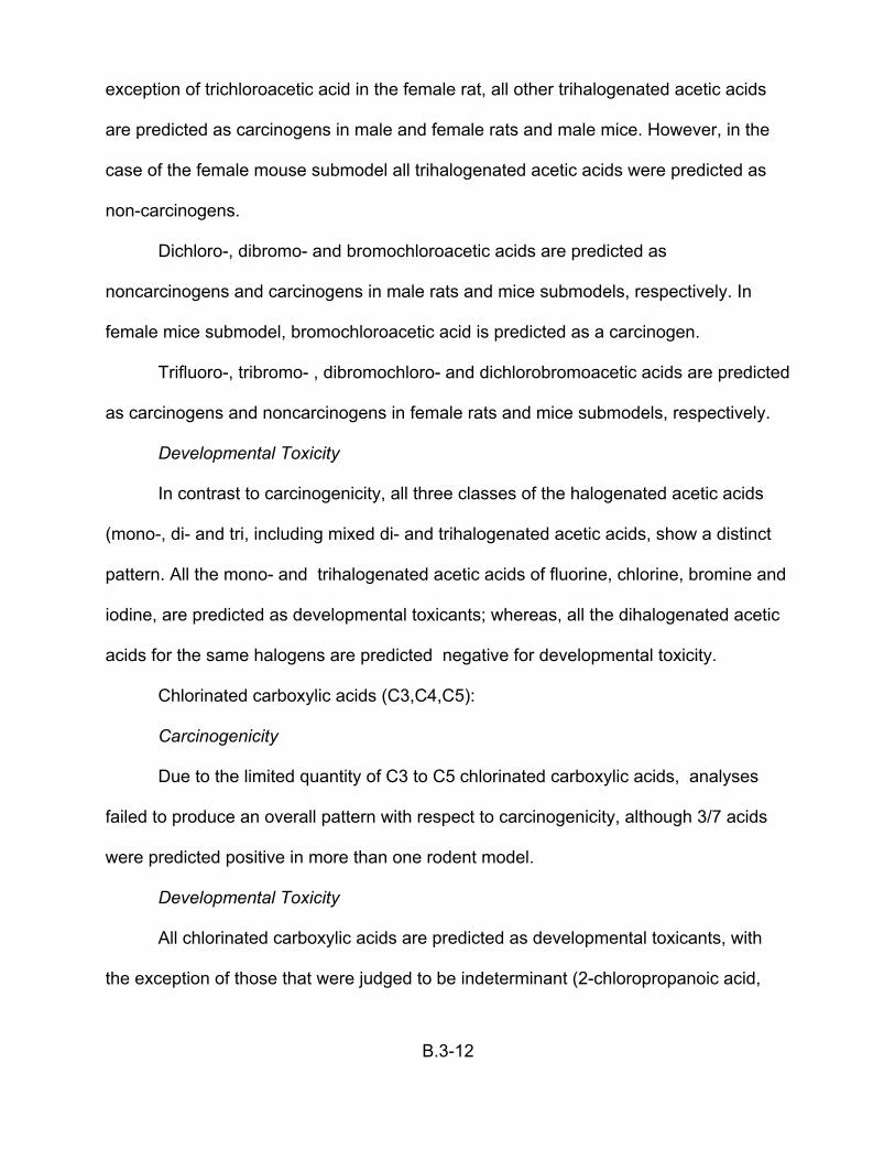
exception of trichloroacetic acid in the female rat, all other trihalogenated acetic acids
are predicted as carcinogens in male and female rats and male mice. However, in the
case of the female mouse submodel all trihalogenated acetic acids were predicted as
non-carcinogens.
Dichloro-, dibromo- and bromochloroacetic acids are predicted as
noncarcinogens and carcinogens in male rats and mice submodels, respectively. In
female mice submodel, bromochloroacetic acid is predicted as a carcinogen.
Trifluoro-, tribromo- , dibromochloro- and dichlorobromoacetic acids are predicted
as carcinogens and noncarcinogens in female rats and mice submodels, respectively.
Developmental Toxicity
In contrast to carcinogenicity, all three classes of the halogenated acetic acids
(mono-, di- and tri, including mixed di- and trihalogenated acetic acids, show a distinct
pattern. All the mono- and trihalogenated acetic acids of fluorine, chlorine, bromine and
iodine, are predicted as developmental toxicants; whereas, all the dihalogenated acetic
acids for the same halogens are predicted negative for developmental toxicity.
Chlorinated carboxylic acids (C3,C4,C5):
Carcinogenicity
Due to the limited quantity of C3 to C5 chlorinated carboxylic acids, analyses
failed to produce an overall pattern with respect to carcinogenicity, although 3/7 acids
were predicted positive in more than one rodent model.
Developmental Toxicity
All chlorinated carboxylic acids are predicted as developmental toxicants, with
the exception of those that were judged to be indeterminant (2-chloropropanoic acid,
B.3-12

and 3,3-dichloropropenoic acid) or outside the Optimum Prediction Space (OPS) [(2,3-
dichloro-4-oxobutenoic acid)].
Nonhalogenated Carboxylic acids:
Carcinogenicity
The majority (21/27) of non-halogenated carboxylic acids were predicted as non-
carcinogens for all four submodels (male/female rats and mice). The exceptions were
glyoxylic acid and 1,2-dioxopropanoic acid, which were predicted as carcinogens in
female mice and rats, 2-oxopropanoic acid, 2-methyl propanoic acid, dioxobutanoic
acid, 4-oxopentanoic acid which were predicted as carcinogens in female rats
submodel, and decanoic acid, undecanoic acid and dodecanoic acid which were
predicted as carcinogens in male rats submodel. Many of these compounds were
judged to be outside the OPS in the male mouse and rat submodels.
Developmental Toxicity
Nonhalogenated carboxylic acids ranging in carbon chain lengths from C2 to C5
are predicted as developmental toxicants, with the exception of 2-oxopentanoic acid,
which is predicted negative. Acids with carbon chain lengths greater than C6 are all
predicted negative, with several of these compounds judged to be outside the OPS.
Di Carboxylic Acids:
Chlorinated Di-Carboxylic Acids:
Carcinogenicity -
As in the case of chlorinated mono-carboxylic acids, there were not enough
chlorinated di-carboxylic acids analyzed to see an overall distinct pattern in prediction.
Developmental Toxicity -
B.3-13
Of the three compounds analyzed, 2-chlorobutenedioc acid is predicted as a
developmental toxicant, chlorobutanedioic acid was predicted as a nondevelopmental
toxicant and 2-chloro-3-methyl-cis-butenedioic acid was predicted as indeterminant.
Nonhalogenated Di-Carboxylic Acids:
Carcinogenicity -
The majority (14/16) of nonhalogenated di-carboxylic acids were gender and
species specific for carcinogenicity, with carcinogenicity limited to the female rat
submodel. These acids were predicted noncarcinogens in male rats and mice and
female mice submodels. Tert-butyl-cis-butenedioic acid and tridecanedioic acid are
exceptions, being predicted as carcinogenic in female mice and noncarcinogenic in
female rats submodels, respectively.
Developmental Toxicity -
Most nonhalogenated di-carboxylic acids (12/16) are predicted as
developmental-toxicants, except octanedioic acid, nonanedioic acid and tridecanedioic
acid, which are predicted negative, and heptanedioic acid which is indeterminate.
Aromatic Carboxylic Acids:
Carcinogenicity -
Aromatic carboxylic acids (7/12) are predicted as carcinogens in the female rat
submodel and noncarcinogens in the male mouse and rat and female mouse
submodels. Three acids (1,2,3-, 1,2,4- and 1,3,5-benzene tricarboxylic acids) are
judged to be outside the OPS in male mice and female rats submodels.
B.3-14
Developmental Toxicity -
All aromatic carboxylic acids are predicted negative for developmental toxicity,
with the exception of phenylacetic acid which is predicted positive.
B.3.2 KETONES
Halogenated Ketones:
Carcinogenicity -
Most halogenated ketones are predicted as carcinogens in the male mouse
submodel and predicted as non-carcinogens in the female mouse and rat and male rat
submodels with the exception of 1-chlorodimethylglyoxal, chloropropanone, 1,1-
dichloropropanone, 1-bromo-1,1-dichloropropanone, 1,1-dichloro-2-butanone and 3,3-
dichloro-2-butanone which are predicted as noncarcinogens in the male mouse
submodel. 1,1,1,3-, 1,1,3,3-tetrachloropropanone and hexachloropropanone are
predicted positive for carcinogenicity in the male rat and 1,1-bromochloropropanone is
predicted positive in female mouse and male mouse. Approximately 50% of these
ketones (19/40) were determined to be outside the OPS.
Developmental Toxicity -
Except for 1,1-dibromoacetone, 1,1-dichloropropanone, 1,1,3-trichloropropanone,
1,1,1,3,3-pentachloropropanone, 1,1-bromochloropropanone, and 1,1-dichloro-2-
butanone, all halogenated ketones are predicted positive for developmental toxicity.
Nonhalogenated Ketones:
Carcinogenicity -
Of the 11 nonhalogenated ketones, most appear to be gender and species
specific for carcinogenicity, in that they are predicted carcinogenic in the male rat
B.3-15

submodel with a few exceptions. These exceptions being, butanone, 3-hexanone and,
6-methyl-5-hepten-3-one which are predicted noncarcinogens. Glyoxal is predicted
positive in the female mouse as well as the male rat submodel. Three compounds are
determined to be outside the OPS for all four submodels.
Developmental Toxicity -
Most nonhalogenated ketones show a positive trend for developmental toxicity.
Geranylacetone and 3-methyl-2,4-hexanedione are judged to be outside the OPS and
3-hexanone, 2,6-dimethyl-2,5-heptadiene-4-one and 6-methyl-5-hepten-3-one are
predicted negative.
Cyclic Ketones:
Carcinogenicity -
All cyclic ketones appear to follow a noncarcinogenic trend in all four submodels,
with only 2,2,4-trichloro-1,3-cyclopentenedione being predicted positive in the female
mouse. 2-Chlorocyclohexanone is determined to be outside the OPS in the male mouse
and 2,6,6-trimethyl-2-cyclohexene-1,4-dione and 1,3,3-trimethyl-1,7-oxabicyclo-[4.1.0]-
heptane-2,5-dione are indeterminant.
Developmental Toxicity -
Of the seven cyclic ketones, four are judged to be outside the OPS, whereas
2,2,4-trichloro-1,3-cyclopentenedione, 2-chlorocyclohexanone and 1,3,3-trimethyl-1,7-
oxabicyclo-[4.1.0]-heptane-2,5-dione are predicted negative for developmental toxicity.
Aromatic Ketones:
Carcinogenicity -
B.3-16
There is no clear pattern evident for carcinogenicity in aromatic ketones. 1-[4-(1-
methylethyl)phenyl]-ethanone and 1,1-(1,4-phenylene)bis-ethanone are predicted
positive in the male mouse and rat submodels, whereas 2,6-tert-butyl-1,4-benzoquinone
is predicted positive in the female mouse submodel and is indeterminant in the male rat
submodel. The remaining aromatic ketones are predicted as noncarcinogens.
Developmental Toxicity -
All aromatic ketones are predicted negative for developmental toxicity.
B.3.3 LACTONES
Carcinogenicity -
The lactones appear to have their carcinogenicity restrained to the male mouse
submodel. Apart from dihydro-4,5-dichloro-2-(3H)-furanone, red-MX, EMX and
4-dodecyl-5-ethyl-2(5H)furanone which are predicted noncarcinogens in the male
mouse and MX which is predicted indeterminant in the male mouse all other lactones
are predicted as carcinogens in the male mouse submodel. 5-Hydroxy-5-
trichloromethyl-2-furanone, BMX-1 and EMX are predicted as carcinogens in the female
mouse submodel. Many of the lactones are judged to be outside the OPS, especially in
the female rat.
Developmental Toxicity -
Most lactones are predicted negative for developmental toxicity. The few
exceptions being 5-hydroxy-5-trichloromethyl-2-furanone, which is predicted
indeterminant, and dihydro-4,5-dichloro-2-(3H)-furanone, red-MX and 4-dodecyl-5-ethyl-
2(5H)furanone, which are judged to be outside the OPS.
B.3-17

B.3.4 ALCOHOLS
Aliphatic Alcohols:
Carcinogenicity -
The number of aliphatic alcohols analyzed is insufficient to indicate a trend in
carcinogenicity. Of the five alcohols analyzed, only 1-[2-(2-methoxy-1-methylethoxy)-1-
methylethoxy]-2-propanol was predicted carcinogenic in the female mouse and male rat
submodels, was predicted noncarcinogenic in the male mouse submodel and was
outside the OPS in the female rat submodel. The remaining alcohols were either
predicted noncarcinogens or were outside the OPS for all four submodels.
Developmental Toxicity -
All the aliphatic alcohols are predicted negative.
Aromatic Alcohols:
Carcinogenicity -
As in the case of aliphatic alcohols not enough aromatic alcohols were analyzed
to realize a trend in carcinogenicity. Most alcohols are predicted as noncarcinogens in
all four submodels with a few exceptions. These exceptions are 2,4,6-trichlorophenol,
which is predicted as a carcinogen in the male mouse; 4-(1-methylethyl)-benzene
methanol, which is predicted positive in the female mouse and female rat submodels;
and 2,6-di-tert-butyl-4-nitrophenol, which is predicted carcinogenic in the male rat
submodel.
Developmental Toxicity -
With the exception of 4-(1-methylethyl)-benzene methanol all aromatic alcohols
are predicted negative.
B.3-18
B.3.5 ETHERS
Aliphatic Ethers:
Carcinogenicity -
The carcinogenic activity is random and spread out for aliphatic ethers, due to
the limited number of compounds analyzed. Bromochloromethyl acetate is predicted as
a carcinogen in the female mouse/rat and male mouse. 1-Chloroethanol acetate is
predicted as a carcinogen in the male rat submodel. 1,2-Dichloroethanol acetate is
predicted as a carcinogen in the female and male mice. 2-Methyl-3,3-dichloro-2-
propenyl dichloromethylether is predicted positive in the female rat. 1,4-Dioxane is
predicted as carcinogenic in female and male mice and male rats, whereas
3-bromopropylchloromethylether is predicted as carcinogenic in all four submodels.
Few compounds are judged to be outside the OPS in various submodels.
Developmental Toxicity -
All aliphatic ethers are predicted negative for developmental toxicity with the
exception of 1-chloroethanol acetate, 3-bromopropylchloromethylether and 1,4-dioxane
which are predicted positive.
Aromatic Ethers:
Carcinogenicity -
The only chemical analyzed for carcinogenicity, 1,4-benzodioxin is predicted a
noncarcinogen in the male mouse, female and male rat submodels. It was determined
to be outside the OPS in the female mouse.
Developmental Toxicity -
1,4-Benzodioxin is predicted negative for developmental toxicity.
B.3-19
B.3.6 NITRILES
Aliphatic Nitriles:
Carcinogenicity -
The carcinogenic potential of most aliphatics nitriles is predicted as negative by
QSAR technique. Carcinogenic activity of aliphatic nitriles seems to be limited to
chlorine and bromine substitutions of single and double carbon chains. Cyanogen
bromide is predicted as a carcinogen in the female rat. Bromoacetonitrile is predicted
positive in female mouse and female rat. Dichloromethyl cyanide is positive in female
mouse. Trichloro- and tribromoacetonitriles are predicted to be carcinogenic in male
rats. Bromochloroacetonirile is predicted as a carcinogen in female and male mice,
trichloropropenenitrile is predicted positive in the female rat. 2,3-Dichloropropanenitrile
and 3,4-dichlorobutanenitrile are predicted as carcinogens in female mice and
3-methylbutane nitrile is predicted positive in the male rat. Few aliphatics nitriles are
determined to be outside the OPS.
Developmental Toxicity -
As in the case of halogenated and short chain carboxylic acids, aliphatic nitriles
show a tendency toward developmental toxicity. With the exception of
bromochloroacetonitrile and 3,4-dichlorobutanenitrile, all other chlorinated and
brominated nitriles are predicted as developmental toxicants. Three chlorine substituted
nitriles, 2,3-dichloropropanenitrile, cis- and trans-2,3,4-trichloro-2-butenenitrile are
determined to be outside the OPS. Of the nonhalogenated nitriles, 3-methylbutane
nitrile is predicted positive and hepatanenitrile is predicted negative for developmental
toxicity.
B.3-20

Aromatic Nitriles:
Carcinogenicity -
The two aromatic nitriles analyzed, are predicted to be noncarcinogenic in all four
submodels.
Developmental Toxicity -
Both aromatic nitriles are predicted negative for developmental toxicity.
B.3.7 AMINES
Aliphatic Amines:
Carcinogenicity -
The number of amines analyzed were too few to recognize a trend in
carcinogenicity. For the two amines analyzed, 1-chloro-3,3,3-trichloro-1-propen-1-amine
is predicted carcinogenic in the female and male mouse submodels, whereas 5-methyl-
3-isoxazolamine is predicted carcinogenic in the male mouse. Both compounds are
predicted as noncarcinogens in the remaining submodels.
Developmental Toxicity -
As in the case of carcinogenicity, no trend can be observed due the fact that only
two compounds were analyzed. 1-Chloro-3,3,3-trichloro-1-propen-1-amine is predicted
positive, whereas 5-methyl-3-isoxazolamine is predicted negative for developmental
toxicity.
Aromatic Amines:
No aromatic amines were analyzed, either for carcinogenicity or developmental
toxicity.
B.3-21
B.3.8 AMIDES
Aliphatic Amides:
Carcinogenicity -
Of the two amides analyzed, 2,2-dichloroacetamide is predicted noncarcinogenic
in three of the four submodels and is determined to be outside the OPS in the female rat
submodel. 2,2,2-Trichloroacetamide is predicted noncarcinogenic in the female mouse
and rat submodels and is predicted carcinogenic in the male mouse and rat submodels.
Developmental Toxicity -
2,2-Dichloroacetamide is predicted indeterminant and 2,2,2-trichloroacetamide is
predicted as a developmental toxicity.
Aromatic Amides:
No aromatic amines were analyzed, either for carcinogenicity or developmental
toxicity.
B.3.9 HALO & NITRO COMPOUNDS
Aliphatic Alkanes and Alkenes:
Carcinogenicity -
The aliphatic alkanes and alkenes have been subdivided into four groups:
1. The group encompassing halogenated (mainly chlorine and bromine) and nitro methanes, show a carcinogenic trend in the male rat submodel, and a noncarcinogenic trend in the other three submodels for the most part. Methyl chloride and bromodichloronitromethane are predicted as indeterminant and bromochloroiodomethane and nitrodibromomethane are predicted as noncarcinogens in the male rats. Methylene chloride is also predicted as a carcinogen in the male mouse. Dibromomethane and bromodichloromethane are predicted positive in all four submodels. Apart from being carcinogenic in the male rat submodel, bromoform is predicted carcinogenic in female rats, dichloroiodomethane is predicted positive in female mice, bromochloroiodomethane and dbromochloromethane are
B.3-22
predicted carcinogenic in female mice and rats and nitrodibromomethane is predicted carcinogenic in the male mouse model. Four of the nitro/halo methanes are determined to be outside the OPS in the female rat submodel.
2. The halogenated and nitro alkanes and alkenes (C2 and greater) are noncarcinogenic with a few exceptions. These exceptions are, 1-chloro-2-ethoxy-2-methoxy ethane, which is predicted as a carcinogen in female and male rats, hexachloroethane is predicted positive in female and male mice and male rats, 1,1,1-tribromo-2-bromo-2-chloroethane is predicted carcinogenic in the female mouse, 3,3,3-trichloro-2-methyl-1-propene is predicted positive in male mice and rats, 2-bromobutane is predicted as a carcinogen in male mice and female rats, 1,1,5,5-tetrachloropentane is predicted carcinogenic in the male rat submodel, 1-hydroxy-3-methyl-2-hexene is predicted positive in female mice and 1-chlorooctane is predicted positive in male rats.
3. Two compounds identified as outliers, undecane and methane sulfonyl chloride are predicted noncarcinogens in all four submodels with the exception of undecane, which is determined to be outside the OPS in male rats.
4. The cyclic halogenated and non-halogenated alkanes and alkenes show no pattern in carcinogenicity. Tetrachlorocyclopropene and hexachlorocyclopentadiene are predicted as a carcinogens in female rats and cyclododecane is predicted positive in the male mouse and rat submodels.
Developmental Toxicity -
Unlike the carcinogenicity model, there is no specific order to toxicity among the
various subgroups. Methylene chloride, dibromomethane, trichloronitromethane,
bromopicrin, bromodichloronitromethane, 1-ethoxy-1-hydroxymethane, 1-nitro-1,1-
dichloroethane, hexachloroethane, 1,2-dichloro-2-methyl butane and methane sulfonyl
chloride are predicted as developmental toxicants, whereas the rest are either predicted
negative, indeterminant or are determined to be outside the OPS.
B.3-23
Aromatic Compounds:
Carcinogenicity -
Most of the aromatic compounds are predicted to be noncarcinogens with a few
exceptions. The few exceptions being, benzene and 1,4-dichlorobenzene which are
predicted to be carcinogenic in female and male mice and male rats.
1,3-Dichlorobenzene and 1,2-bis(1-methylethenyl)benzene are predicted positive in the
female mouse submodel and, toluene is predicted to be carcinogenic in female rats.
Some of these compounds are predicted to be indeterminant or determined to be
outside the OPS.
Developmental Toxicity -
All aromatic compounds are predicted negative for developmental toxicity with
the exception of benzene which is determined to be outside the OPS and,
1,4-dichlorobenzene which is predicted as indeterminant.
B.3.10 CONCLUSIONS
In addition to our initial agreement with OW of prioritizing the list of DBPs in
terms of potential carcinogenicity and developmental toxicity based on probability,
NCEA-Cincinnati has categorized these DBPs by chemical class based on functional
groups. Based on these classifications, patterns of prediction have been identified that
should aid OW in eliminating certain chemical classes based on functional groups.
However, in contrasting these predicted data with the available literature, one must
follow the criteria used to develop the respective models for all literature published
before and after model development. It should be well understood that all QSAR models
are closed systems and ultimately should not be used to replace bioassays. However,
B.3-24
QSAR predictions are independent of equilibrium changes that are pH dependent, such
as the activity of MX compounds at different pH’s in the Ames mutagenicity assay.
Using QSAR the authors have been able to distinguish the mutagenic potential of the
closed (lactone) and open forms of MX compounds which is not possible under Ames
assay conditions.
Developmental toxicity was identified as a health-related endpoint common to the
majority of aliphatic mono- and dicarboxylic acids; most aliphatic halogenated and non-
halogenated ketones and most aliphatic haloacetonitriles. In the case of the NTP
carcinogenicity submodels, most aliphatic aldehydes were identified as likely
carcinogens only in the female mouse submodel. The majority of the aliphatic and
aromatic dicarboxylic acids were identified as likely carcinogens in the female rat
submodel. All other functional groups were for the most part predicted as
noncarcinogens in all NTP cancer submodels (male/female rats and mice). An analyses
of these QSTR/DBPS results should aid in the prioritization of chemicals to evaluate for
these health-related endpoints in the absence of in vivo bioassays.
Additional research will include an investigation of which features (descriptors) in
a molecule for various chemical classes are responsible for the positive and/or negative
predictions and why? In addition, all “similarity search” data for each model and
chemical class will be reviewed with the idea of identifying those compounds in the data
base that are most similar electronically (in terms of descriptor contribution) to the query
compounds and why. Hopefully, this type of information will extend our knowledge and
understanding of the structural basis for activity within these classes, whereas a simple
B.3-25
list of TOPKAT predictions provides no such insight. Lastly, the authors welcome the
opportunity to compare their results to those obtained by other QSAR models.
REFERENCES
Gombar, V.K. 1995. Assessment of developmental toxicity potential of chemicals by qualitative structure-toxicity relationship models. Chemosphere. 31:2499-2510.
Gombar, V.K. 1998. Quantitative structure-activity relationship in toxicology: From fundamentals to applications. In: Advances in Molecular Toxicology, C. Reiss et al., Ed. VSP Publishers, Utrecht, Netherlands. p. 125-139.
Gombar, V. K. et al. 1997. Quantitative Structure-Activity Relationships in Predicting Chemical Toxicity: When is the Prediction Reliable, Proceedings of the 7th International Workshop on QSARs in Environmental Science. 27:399-411.
HDI. 1995. TOPKAT 3.0 Reference manual, Health Designs Inc., 183 East Main Street, Rochester, New York 14604.
B.3-26
APPENDIX B.4 SUMMARY OF DBP-SPECIFIC TOXICITY DATA
B.4.1 SELECTION OF COMPOUNDS FOR EVALUATION
The selection of treatment trains for consideration was one factor in the
determination of which DBPs were investigated. We have focused on DBPs identified in
a split-sample treatment study of Ohio River water (Miltner et al., 1990).
B.4.2 INDIVIDUAL CHEMICAL SUMMARIES
The goal of this section is to present chemical summaries for several
demonstrative chemicals. Due to logistical constraints of this document, and because
such summaries for other chemicals may be presently available, the chemicals
summarized here are only examples of the toxicologic data that are available on the
DBPs. Full chemical summaries should be compiled for the DBPs pertinent to decisions
using the CRFM. We have focused our evaluation on compounds previously identified
under a pilot-scale investigation conducted and previously reported (Miltner et al., 1990;
see Table B.4-1). Although bromate levels were not measured in Miltner et al. (1990),
this risk assessment used levels measured by Miltner et al. (1992).
The following summaries provide pertinent details of the chemicals for focus in
this comparison. While more exhaustive reviews are available for some compounds,
and more data are available for some than others, these sections highlight the important
points for consideration. Because of the primary importance of the oral route of
exposure for DBPs in drinking water, we have not addressed regulatory concern for
exposures other than oral, unless specifically applicable or dictated by lack of orally-
relevant data. In reporting reproductive and developmental effects, we have included
some data available with whole-embryo culture studies, an in vitro design whose results
B.4-1

are not deemed applicable in determining regulatory levels (e.g. RfD) of exposure.
They are, nonetheless, useful in estimating the potential for such an effect to occur in
vivo.
TABLE B.4-1
EPA - Verified Data Available for Compounds Evaluated in this Case Study
Compound [CASRN] RfD Carcinogenic Risk
Oral Slope Unit Risk Chloroform [67-66-3] Bromodichloromethane [75-27-4] Dibromochloromethane [124-48-1] Bromoform [75-25-2] Trichloroacetic Acid [76-03-9] Dichloroacetic Acid [79-43-6] Chloroacetic Acid [79-08-3] Chloral Hydrate [75-87-6] Potassium Bromate [7758-01-2]
1 E–2 mg/kg/day (09/01/92)
2 E–2 mg/kg/day (03/01/91)
2 E–2 mg/kg/day (03/01/91)
2 E–2 mg/kg/day (03/01/91)
1 E-1 mg/kg/day (05/06/93)
4 E-3 mg/kg/day (06/15/93)
2 E–3 mg/kg/day (02/01/96)
2 E-3 mg/kg/day (02/01/96)
N/A
6.1 E–3 1.7 E-7(03/01/91)
6.2 E-2 (03/01/91)
1.8 E-6
8.4 E-2 (01/01/92)
2.4 E-6
7.9 E-3 (01/01/91)
2.3 E- 7
N/A N/A
N/A N/A
N/A N/A
N/A (?) N/A (?)
4.9 E-1 (12/11/92)
1.4 E-5
Trihalomethanes: The early identification of carbon tetrachloride as a potent
liver carcinogen may have heightened the concerns over finding chloroform in drinking
water supplies in 1974. This finding stimulated research on THMs which has focused
on dose-response relationships, exposure estimates for humans, biomarkers of
exposure, and studies of the mechanism(s) underlying cancer. These efforts have
spread to other halomethane compounds, resulting in reduced uncertainty about toxicity
B.4-2

data generated in rodent species. However, the differences in response noted with
different dose regimens/schedules and vehicles complicate the extrapolation of some
responses following the administration of bolus doses of THMs. The EPA’s Science
Advisory Board reviewed the Office of Water’s draft Drinking Water Criteria Document
(October 25-26, 1990) and advised that the concern over corn oil as vehicle for gavage
studies dictated that the hepatocarcinogenic effects (as noted with chloroform) should
be utilized only in making a weight-of-evidence classification, and should “be
disregarded in making a quantitative estimation of the carcinogenic risk of a
trihalomethane.” The IRIS file for all three brominated THMs (revised 03/01/91) states
that, “No adequate data on the teratogenic or reproductive effects of trihalomethanes
are available”, but the IRIS file for chloroform (revised 09/01/92) does not contain such
a statement.
Chloroform (CHCl3): Chloroform is the THM which has received the most
attention. Care should be taken that chloroform data are not extrapolated without
specific and detailed justification. A weight-of-evidence classification of B2 (probable
human carcinogen) has been assigned to chloroform. There are no epidemiologic
studies for chloroform itself, although chloroform was the major identified DBP in
epidemiologic studies which have associated increased incidences of rectal, bladder
and colon cancer with drinking water chlorination. Chloroform induces CNS depression
and cardiac sensitization, though at doses not likely encountered in drinking water (Bull
and Kopfler, 1991). Chloroform is considered highly fetotoxic, but not teratogenic
(Schwetz et al., 1974 and Thompson et al., 1974 in U.S. EPA, 1998a); and inhalation
exposure produced a dose-dependent increase in post-implantation death and reduced
B.4-3
crown-rump length and weight gain in rat pups (ATSDR, 1996). Savitz et al. (1995)
used data from case-controlled studies on miscarriages, preterm delivery and low birth
weight as related to THM concentration in drinking water to demonstrate that although
no dose-response was observed, a significant elevation of miscarriage was present in
the highest sextile of THM concentration. Increased association (odds ratios >1.50) of
adverse birth outcomes which included low birth weight, "CNS defects", cleft palate and
cardiac defects (Bove et al., 1995).
CHCl3: The oral RfD (revised 09/01/92) is based on the finding of fatty cysts in
liver of dogs chronically exposed to chloroform in toothpaste (Heywood et al., 1979),
and demonstrated a LOAEL of 15 mg/kg/day, which was converted to 12.9 mg/kg/day
when dosing schedule was converted to 7 days/week (U.S. EPA, 1998a). Application of
uncertainty and modifying factors totaling 1,000 reduce the oral RfD to 10 :g/kg/day
(700 :g/day for a 70 kg human). For carcinogenic risk (updated 03/01/91), an oral
slope factor of 6.1x10E-3 per mg/kg/day and a drinking water unit risk of 1.7x10E-7 per
:g/L have been assigned to chloroform. A carcinogenic risk of 1.0x10E-6 results from
exposure to a concentration of 6 :g chloroform/L drinking water.
Bromodichloromethane (BDCM): A weight-of-evidence classification of B2
(probable human carcinogen) has been assigned to BDCM. BDCM produces tumors at
multiple sites in multiple species, and the kidney tumors produced are independent of
alpha-2-micro-globulin. There are no epidemiologic studies for BDCM alone, although
ecologic and epidemiologic studies which have associated increased incidences of
rectal, bladder and colon cancer with drinking water chlorination. Because of the
complex mixture of DBPs in drinking water and the co-exposure to other factors which
B.4-4
modify cancer formation, these data are insufficient for assessing the carcinogenic risk
of BDCM to humans. BDCM is reported to be mutagenic in several in vitro evaluations
and is structurally similar to other known animal carcinogens. Klinefelter et al. (1995)
reported that the exposure of rats to BDCM in drinking water (at 39 mg/kg/day) sperm
velocity was significantly decreased.
BDCM: The oral RfD (revised 03/01/91) is based on the finding of renal
cytomegaly in micechronically exposed to BDCM via gavage in corn oil (NTP, 1986),
which demonstrated a LOAEL of 17.9 mg/kg/day (U.S. EPA, 1998a). Application of
uncertainty and modifying factors totaling 1,000 reduced the oral RfD to 20 :g/kg/day
(1400 :g/day for a 70 kg human). For carcinogenic risk (revised 03/01/93), an oral
slope factor of 6.2x10E-2 per mg/kg/day and a drinking water unit risk of 1.8x10E-6 per
:g/L have been assigned to BDCM, based on the “linearized multistage model, extra
risk”. A carcinogenic risk of 1.0x10E-6 results from exposure to a concentration of 0.6
:g BDCM/L drinking water.
Dibromochloromethane (DBCM): A weight-of-evidence classification of C
(possible human carcinogen) has been assigned to DBCM. There are no epidemiologic
studies for DBCM alone, although ecologic and epidemiologic studies have suggested
increased incidences of rectal, bladder and colon cancer associated with drinking water
chlorination. DBCM is mutagenic and carcinogenic in male and female mice, however,
liver tumors are found only at levels of DBCM which produced liver damage and only
with corn oil as vehicle. The IRIS file for all three brominated THMs (revised 03/01/91)
states that, “No adequate data on the teratogenic or reproductive effects of
trihalomethanes are available”, but the IRIS file for chloroform (revised 09/01/92) does
B.4-5

not contain such a statement. However, a study by Ruddick et al. (1983) evaluated the
developmental toxicity of some THMs. Unfortunately, the low number of fetuses
examined from DBCM-exposed dams did not allow the developmental toxicity of DBCM
to be confirmed or refuted.
DBCM: The oral RfD (revised 03/01/91) is based on the finding of hepatic
lesions in rats exposed subchronically via corn oil gavage (NTP, 1985), which
demonstrated a NOEL of 30 mg/kg/day, which was converted to 21.4 mg/kg/day (U.S.
EPA, 1998a). A LOAEL of 60 mg/kg/day was observed, which converted to 42.9
mg/kg/day. Application of uncertainty and modifying factors totaling 1,000 (to the
NOEL) reduce the oral RfD to 20 :g/kg/day (1400 :g/day for a 70 kg human). For
carcinogenic risk (revised 01/01/92), an oral slope factor of 8.4x10E-2 per mg/kg/day
and a drinking water unit risk of 2.4x10E-6 per :g/L have been assigned to DBCM. A
carcinogenic risk of 1.0x10E-6 results from exposure to a concentration of 0.4 :g
DBCM/L drinking water. There are no published data on teratogenicity or reproductive
effects of trihalomethanes (IRIS, 1998; updated 03/01/91), however, BDCM produced
dose-dependent skeletal malformations in rats (Ruddick et al., 1983).
Bromoform (CHBr3): A weight-of-evidence classification of B2 (probable
human carcinogen) has been assigned to chloroform. There are no epidemiologic
studies for bromoform itself, although ecologic and epidemiologic studies have
suggested increased incidences of rectal, bladder and colon cancer associated with
drinking water chlorination. Geographic studies have suggested correlations between
the levels of trihalomethanes in drinking water and incidences of bladder, colon, rectal
and pancreatic cancer in humans. Interpretation of these studies is complicated due to
B.4-6
the study design which did not allow for the consideration of other factors which modify
carcinogenic response. Bromoform is genotoxic and induced colorectal tumors in mice
following intraperitoneal administration and tumors in rats following oral administration.
There are no adequate published data on teratogenicity or reproductive effects of
trihalomentanes (U.S. EPA, 1998a; chronic oral RfD for bromoform was updated on
03/03/91), although bromoform (and BDCM) produced a dose-dependent increase in
skeletal malformations in rats (Ruddick et al., 1983).
CHBr3: The oral RfD (revised 03/01/91) is based on the finding of hepatic
lesions in rats exposed subchronically by gavage (NTP, 1989), which demonstrated a
NOEL of 25 mg/kg/day, which was converted to 17.9 mg/kg/day (U.S. EPA, 1998a).
Application of uncertainty and modifying factors totaling 1,000 reduce the oral RfD to 20
:g/kg/day (1400 :g/day for a 70 kg human). For carcinogenic risk (revised 01/01/91),
an oral slope factor of 7.9x10E-3 per mg/kg/day and a drinking water unit risk of
2.3x10E-7 per :g/L have been assigned to bromoform. A carcinogenic risk of
1.0x10E-6 results from exposure to a concentration of 4 :g bromoform/L drinking water.
Haloacetic Acids: The primary exposure to TCA and DCA is through drinking
water. While these are the only two HAAs for which an IRIS file exists, and they are the
most commonly encountered HAA DBPs, their carcinogenic dose-response curves are
dissimilar. TCA produces a linear dose-response for liver tumors, while that for DCA
demonstrates a distinct dose level, below which tumors are not observed. TCA, DCA
and the other HAA DBPs were assessed for in vitro developmental effects. Rogers et
al. (1995) removed mouse conceptuses (at the 3 to 6 somite stage) and subjected them
to whole embryo culture in the presence of mono-, di- and tri-brominated and
B.4-7
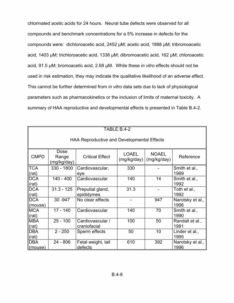
chlorinated acetic acids for 24 hours. Neural tube defects were observed for all
compounds and benchmark concentrations for a 5% increase in defects for the
compounds were: dichloroacetic acid, 2452 :M; acetic acid, 1888 :M; tribromoacetic
acid, 1403 :M; trichloroacetic acid, 1336 :M; dibromoacetic acid, 162 :M; chloroacetic
acid, 91.5 :M; bromoacetic acid, 2.68 :M. While these in vitro effects should not be
used in risk estimation, they may indicate the qualitative likelihood of an adverse effect.
This cannot be further determined from in vitro data sets due to lack of physiological
parameters such as pharmacokinetics or the inclusion of limits of maternal toxicity. A
summary of HAA reproductive and developmental effects is presented in Table B.4-2.
TABLE B.4-2
HAA Reproductive and Developmental Effects
Dose Range
(mg/kg/day) Critical Effect LOAEL
(mg/kg/day) NOAEL
(mg/kg/day) Reference
330 - 1800 Cardiovascular, 330 - Smith et al., 1989eye
140 - 400 Cardiovascular 140 14 Smith et al., 1992
31.3 - 125 Preputial gland, epididymes
31.3 - Toth et al., 1992
30 -947 No clear effects - 947 Narotsky et al., 1996
17 - 140 Cardiovascular 140 70 Smith et al., 1990
25 - 100 Cardiovascular / craniofacial
100 50 Randall et al., 1991
2 - 250 Sperm effects 50 10 Linder et al., 1995
24 - 806 Fetal weight, tail defects
610 392 Narotsky et al., 1996
TCA (rat) DCA (rat) DCA (rat) DCA (mouse) MCA (rat) MBA (rat) DBA (rat) DBA (mouse)
CMPD
B.4-8

Trichloroacetic Acid (TCA): A weight-of-evidence classification of C (possible
human carcinogen) has been assigned to TCA. This has its basis in a lack of human
data and the production of tumors in male and female mice, but there is no evidence of
carcinogenicity in rats. Genotoxic evaluations have produced mixed results, and TCA
does not appear to induce point mutations. No epidemiologic studies have shown an
association between exposure to TCA and the production of site-specific tumors. Smith
et al. (1989) report a LOAEL of 330 mg/kg/day for developmental effects (resorption,
heart and eye defects, decreased fetal weight gain and reduced maternal weight gain)
in rats.
TCA: The oral RfD for TCA was not established during the revision
accomplished on 01/01/94 (U.S. EPA, 1998a). No quantitative estimates of
carcinogenic risk from oral exposure to TCA were established during the revision of the
Carcinogenesis Assessment section of IRIS (08/04/93) (U.S. EPA, 1998a). The
Agency is exploring the development of a biologically-based model to accommodate the
existing database and other data under development.
Dichloroacetic Acid (DCA): A weight-of-evidence classification of B2 (probable
human carcinogen) has been assigned to DCA. This is based on a lack of human
carcinogenicity data and an increased incidence of hepatocellular adenoma and
carcinomas in female mice. Nodules expected to progress into hepatocellular
adenomas and carcinomas were also increased in both rats and mice. No
epidemiologic studies have shown an association between exposure to TCA and the
production of site-specific tumors. Smith et al. (1992) reported a NOAEL of 14
mg/kg/day for developmental (cardiac) defects.
B.4-9

DCA: An oral RfD is not available on IRIS at this time. There are no quantitative
estimates of carcinogenic risk from oral exposure to DCA available at this time (U.S.
EPA, 1998a). The Agency is exploring the development of a biologically-based model
to accommodate the existing database and other data under development. A
subchronic (14-day) dose of 25 mg/kg dose of BAA produced adverse effects on
epididymal sperm morphology or histology.
Chloroacetic Acid (MCA): MCA in drinking water at concentrations of up to
1100 mg/L (time-averaged concentration) did not produce liver tumors, pathology,
peroxisome or hepatocyte proliferation, or alterations of serum enzymes. Chronic (104
week) exposure of rats to MCA produced increased spleen weights in all doses 3.5 to
59.9 mg/kg/day) (DeAngelo et al., 1997).
Bromochloroacetic Acid (BCA): The only available published findings with
BCA involve a drinking water exposure (21 days) to male mice. Parrish et al. (1996)
demonstrated that BCA and DBA produce oxidative stress in liver tissue, as evidenced
by hydroxylated DNA adducts, while TCA and DCA do not. The authors suggest that
oxidative damage may modulate chronic toxicity associated with brominated HAAs.
Bromoacetic Acid (MBA): Regulatory levels and toxicity assessments for
bromoacetic acid are not available on IRIS. Randall et al. (1991) gavaged pregnant rats
with MBA in distilled water and noted a LOAEL of 100 and a NOAEL of 50 mg/kg/day
for developmental effects including cardiovascular and craniofacial defects.
Dibromoacetic Acid (DBA): A single dose of 1250 mg/kg DBA produced
significant alterations in sperm motility, abnormal sperm head morphology and flagellar
degeneration, decreased sperm counts (85% of control) in caput epididymus and
B.4-10
decreased serum testosterone (17% of control). Subsequent studies of DBA with male
rats indicated a subchronic NOAEL of 10 mg/kg/day with respect to sperm motility of
fertility (Linder et al., 1995). Narotsky et al. (1996) reported a delay in partutition in mice
administered DBA by gavage in water; the effect was produced by all doses of DBA (24
to 806 mg/kg/day) and in a dose-dependent manner.
Haloacetonitriles (HANs): As a group, the data base for haloacetonitriles is not
as rich as that for trihalomethanes of haloaceto acids. Due to this constraint, the data
presented in this section are combined for ease of presentation.
HAN Toxicity: The target organ(s) for HANs have not been established.
Subchronic (90-day) studies with rats dosed via gavage using corn oil vehicle (Hayes et
al., 1986) have been performed with DCAN and DBAN. Critical effects of increased
liver weight (DCAN) and decreased body weight gain (DBAN) were identified. A
NOAEL for DCAN was established at 8 mg/kg/day and a NOAEL for DBAN was
established at 6 mg/kg/day. No such values are available for the other HANs.
Application of uncertainty factors of 3,000 to these NOAEL values produce “provisional
RfDs” of 3x10E-3 mg/kg/day for DCAN and 2x10E-3 mg/kg/day for DBAN. These
values generally agree with provisional reference doses from reproductive and
developmental toxicity studies Table B.4-3.
All compounds except DBAN (drinking water) were administered in TCAP via
gavage to Long-Evans rats over GD 6-18. Values derived from TCAP-based doses
may produce somewhat conservative estimates of risk because TCAP stimulates a
higher delivery of HANs to the fetus than does corn oil (Gordon et al., 1991).
B.4-11
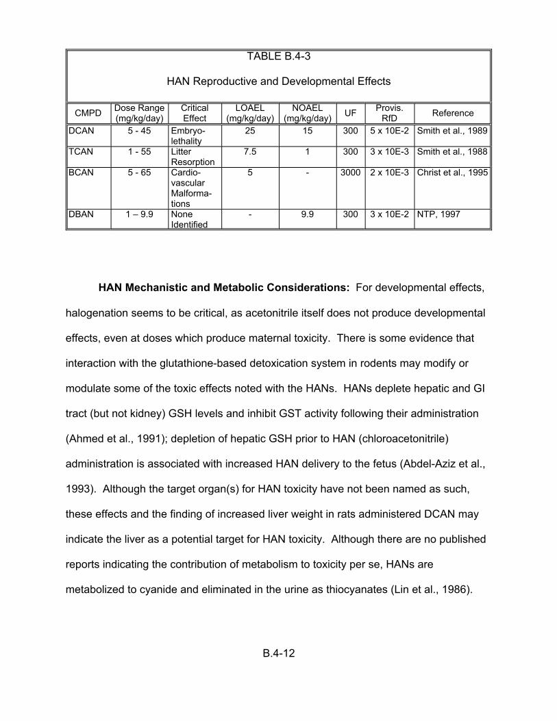
TABLE B.4-3
HAN Reproductive and Developmental Effects
CMPD Dose Range (mg/kg/day)
Critical Effect
lethality TCAN 1 - 55 Litter
Resorption 7.5 1
BCAN 5 - 65 Cardio-vascular Malforma-tions
5 -
DBAN 1 – 9.9 None Identified
- 9.9
LOAEL NOAEL (mg/kg/day) (mg/kg/day)
DCAN 5 - 45 Embryo- 25 15 300 5 x 10E-2
300 3 x 10E-3
3000 2 x 10E-3
UF Provis. RfD Reference
Smith et al., 1989
Smith et al., 1988
Christ et al., 1995
300 3 x 10E-2 NTP, 1997
HAN Mechanistic and Metabolic Considerations: For developmental effects,
halogenation seems to be critical, as acetonitrile itself does not produce developmental
effects, even at doses which produce maternal toxicity. There is some evidence that
interaction with the glutathione-based detoxication system in rodents may modify or
modulate some of the toxic effects noted with the HANs. HANs deplete hepatic and GI
tract (but not kidney) GSH levels and inhibit GST activity following their administration
(Ahmed et al., 1991); depletion of hepatic GSH prior to HAN (chloroacetonitrile)
administration is associated with increased HAN delivery to the fetus (Abdel-Aziz et al.,
1993). Although the target organ(s) for HAN toxicity have not been named as such,
these effects and the finding of increased liver weight in rats administered DCAN may
indicate the liver as a potential target for HAN toxicity. Although there are no published
reports indicating the contribution of metabolism to toxicity per se, HANs are
metabolized to cyanide and eliminated in the urine as thiocyanates (Lin et al., 1986).
B.4-12
Halide displacement or oxidation of a hydrogen atom via mixed function oxidase to
produce a hydroxyacetonitrile has been proposed to account for cyanide liberation.
Miscellaneous Compounds
1,1,1-Trichloropropanone (1,1,1-TCP): 1,1,1-Trichloropropanone
(trichloronitromethane; 1,1,1-TCP) is one of the less well-studied DBPs. 1,1,1-TCP is
mutagenic in vitro, and the mutagenicity of related compounds decreases with
increasing degree of chlorination, and is lower for chlorinated than for brominated
analogs.
Chloropicrin (CP): Chloropicrin is the most acutely toxic of the DBPs examined
in this document. Few studies on its long-term toxicity (e.g. carcinogenicity, NCI, 1978)
have been successfully completed, owing to lethality. In vitro tests have demonstrated
CP’s mutagenic potential (gene reversion, primary DNA damage and the induction of
sister chromatid exchanges in human lymphocytes. Paucity of reported details
precludes the quantitative use of developmental toxicity findings (decreased fetal
weight) in rats and rabbits. The acute (4-hour) toxicity of CP is evidenced by temporally
biphasic lethality, with animals expiring either within 24 hours, or at approximately 10
days. The LC50 for CP (12 ppm) approximates that of phosgene. A 13-week exposure
of rats to CP by inhalation identified the lung as the primary organ for toxicity (dose-
dependent increases in weight and bronchiolar lesions), and identified 0.67 ppm CP as
a NOAEL . The relevance of lung as target organ for inhalation exposures is supported
by a report of lacrymation, respiratory distress, coughing and bronchitis in humans
inhabiting a house which had been previously fumigated with CP (measured
concentration of CP was 48 ppb). Exposure of rats to CP via gavage in a 90-day study
B.4-13
produced lethality, which was attributed to pulmonary complications from CP aspiration,
and necrosis of the stomach as the primary histopathological finding with a NOAEL of 8
mg/kg/day. Although lung was evaluated, no adverse effects were noted at doses of up
to 32 mg/kg/day. Together, these data may indicate that CP’s toxic is directed at the
portal of entry.
Chloral Hydrate (CH): This agent has not been evaluated by the U.S. EPA for
evidence of human carcinogenic potential. Sallenfait et al. (1995) exposed chloral
hydrate (0, 0.5, 1.0, 1.5, 2.0 and 2.5 mM) to rat embryos in in vitro whole embryo culture
and noted dose-dependent effects such as decreased crown-rump length, head length
and number of somites at doses above 0.5 mM.
CH: The oral RfD (revised 02/01/96) is based on the finding of hepatotoxicity in
mice exposed subchronically via drinking water (Sanders et al., 1982), which
demonstrated a LOAEL of 15.7 mg/kg/day (U.S. EPA, 1998a). Application of
uncertainty and modifying factors totaling 10,000 (to the LOAEL) reduce the oral RfD to
2 :g/kg/day (140 :g/day for a 70 kg human). Carcinogenic risk for CH has not been
established (U.S. EPA, 1998a).
Potassium Bromate (Bromate): To date there have been no surveys reporting
concentrations of bromate in drinking water. However, several laboratory and bench-
scale pilot treatment studies have identified factors which contribute to the formation of
bromate. Drinking water studies with rats have shown the production of kidney tumors
(males and females) and peritoneal mesotheliomas (males only) (Kurokawa et al.,
1983). While these results indicate that bromate is a complete carcinogen, additional
experiments in this study demonstrated its tumor promoting activity in the kidney, and
B.4-14
demonstrated that the lowest dose producing kidney tumors was 6.5 mg/kg/day (doses
employed were 0.7, 1.3, 2.5, 5.6, 12.3 and 33.4 mg/kg/day). Interestingly, there was no
increase in liver tumors following initiating treatment (with EHEN). Kurata et al. (1992)
treated rats with acute doses of bromate followed by promoting doses of barbital sodium
to examine tumor initiating activity, but could demonstrate none. The lack of tumor
initiating activity may support that longer doses are necessary to initiate tumors or that
bromate produces renal tumors through promotional activity. An evaluation of the
impact of bromate (either KBrO3 or NaBrO3) indicates that these chemicals, but not KBr
induce alpha-2-micro-globulin accumulation in the kidneys of male, but not female, rats
(Umemura et al., 1993). These data, coupled with the lack of renal carcinogenicity in
mice and hamsters (Kurokawa et al., 1986b; Takamura et al., 1986b), raise the question
of the relevancy of bromate-induced renal tumors to the evaluation of cancer risk in
humans. The involvement of alpha-2-micro-globulin as an exclusive mechanism of
tumorigenicity in rat kidneys is confounded by the finding of renal tumors in female rats
(Kurokawa et al., 1983). Alternately, the production of oxidative stress in renal tissue
may stimulate cell replication, resulting in tumor promotion (Umemura et al., 1995).
Although the finding of renal tumors in female rats may reduce the perceived
importance of alpha-2-micro-globulin as an event modifying renal carcinogenicity, its
association with male rat kidney tumors may indicate that the mechanism may increase
the incidence of tumors in male rats beyond the incidence in female rats. This may
raise questions about the validity of carcinogenic risk estimates for bromate, as they are
mainly based on the incidence and dose-response relationship demonstrated for male
rat kidney tumors. Consistent with the finding of renal toxicity in rodents, humans
B.4-15
acutely exposed to bromate (potassium and/or sodium bromate) in permanent hair
wave neutralizing solutions have demonstrated severe renal damage as well as
permanent hearing loss. There are no available published reports on the potential of
bromate to produce developmental toxicity. Recently, published data (DeAngelo et al.,
1998) have confirmed the multi-site carcinogenicity of bromate (in rats). A slight dose-
response was noted for kidney tumors in mice. The U.S. EPA (1998a) has considered
this evidence supportive of earlier MCL (0.01 mg/L) and MCLG (zero) values.
B.4-16

APPENDIX C-1
Human Data on Health Risks from Exposure to Disinfected Drinking Water: Epidemiologic Studies of Cancer and Reproductive/Developmental Effects

Both epidemiological and toxicological methods have been used to assess
human health risks from exposure to disinfected drinking water. Results from
experiments in animals must be extrapolated from exposures that are several orders of
magnitude higher than actual human exposures, and synergistic and antagonistic
effects of mixtures of chemicals are not taken into account when evaluating the
carcinogenic risks of individual DBPs. Epidemiology offers the opportunity to study
directly mixtures of chemicals at relevant exposures in humans. The studies must be
properly designed, conducted with minimal systematic bias, and should be sufficiently
large to provide information to confidently judge the impact of observed associations.
Since the early 1970’s, a large number of epidemiologic studies of varying design
and quality have been published in the scientific literature. The studies have focused
almost exclusively on chlorinated drinking water and its association with cancer rather
than on individual chemical exposures. Reproductive and developmental epidemiologic
studies on this topic first appeared in the literature in the late 1980’s. However, only
recently have investigators collected information to quantitatively estimate exposures to
individuals from different chemical families and species of DBPs and begun to study
disinfectants other than chlorine.
The purpose of this section is to provide a brief overview of the existing
epidemiologic literature suggesting a potential hazard from exposure to disinfected
drinking water and its associated DBPs.
C.1 CANCER STUDIES
Several types of epidemiological studies have been conducted to assess the
association between cancer and chlorinated drinking water. Ecological (Harris, 1974;
Page et al., 1976; Cantor et al., 1978; Hogan et al., 1979; Carlo and Mettlin, 1980;
C1-1
Tuthill and Moore, 1980; Wigle et al., 1986; Flaten, 1992), cohort (Wilkins and
Comstock, 1981; Doyle et al., 1997), and case-control designs (e.g., Brenniman et al.,
1980; Cragle et al., 1985; Gottlieb et al., 1981, 1982; Cantor et al., 1987, 1998;
Ijsselmuiden et al., 1992; McGeehin et al., 1993; King and Marrett, 1996; Hildesheim et
al., 1998; Young et al., 1987) have evaluated both incident and decedent cases. These
studies differ in their basic approach and the evidence they can provide about the
possible causality of an epidemiological association between chlorinated drinking water
and cancer. These studies are not reviewed in detail in this document. However, a
summary of the more methodologically sound studies, e.g, those based on incident
cases, and having interviews and individual exposure estimates, is provided in Appendix
C.2.
Because meta-analytic methods can be used to quantitatively summarize a body
of literature and provide a single point estimate of effect for a body of literature, it seems
logical to pursue such an estimate for application in this cost effectiveness case study.
In an attempt to quantitatively review the literature, Morris et al. (1992) presented an
aggregate meta-analysis of the published epidemiologic literature relating to water
chlorination and cancer. They identified 10 articles published between 1966 and 1991
that evaluated exposure to chlorinated water and cancer at the level of the individual
(ecological studies were excluded). The authors of these 10 articles evaluated a dozen
different cancer sites and reported overall odds ratios (OR) ranging from less than one
to almost three. The cancer sites most frequently examined were bladder and colon (7
articles each), followed by stomach, rectum, and pancreas (6 articles each). Morris et
al. generated summary (weighted average) OR and 95% confidence interval estimates
for each of the 12 cancer sites and reported significantly elevated ORs of 1.21 (95% CI
C1-2
= 1.09-1.34) and 1.38 (95% CI = 1.01-1.87) for bladder and rectal cancer, respectively.
The OR for all cancer sites combined was reported to be 1.15 (95% CI = 1.09-1.20).
At the request of U.S. EPA, this work was independently evaluated and
reanalyzed by Dr. Charles Poole of Boston University (Poole, 1997). Poole found that
there was considerable heterogeneity among these data and that there was evidence of
publication bias within this body of literature. He also found that the aggregate
estimates reported by Morris et al. (1992) were unstable and were sensitive to
reasonable changes in the analytical methods and to the addition or deletion of a single
study. For these and other reasons, Poole recommended that these data not be
combined into a single summary estimate and that they had limited utility for risk
assessment purposes. Furthermore, he concluded that the issue of whether or not
water chlorination caused cancer was still an open question (Poole, 1997). Because of
these findings, a summary OR from which probabilities of cancer occurrence in relation
to DBP exposure could be derived is not currently available, and has not been used in
the current case study. Several additional studies of cancer and exposure to D/DBPs
have been published since the conclusion of the analysis by Poole. The U.S. EPA is
currently developing a further quantitative analysis of the available epidemiologic
literature which is designed to include an updated literature search extended to the
present time and an evaluation of the body of relevant studies on the basis of more
meaningful exposure groupings. Of particular interest will be creating study groupings
formed from the perspective of the type of source water, specific treatment
technologies, and type and amount of the specific chemical byproducts present in the
delivered water. If the epidemiologic studies can be meaningfully categorized and
summarized in this way (including the determination that aggregation of study results is
C1-3
appropriate), the human data can be used in future applications of this cost
effectiveness methodology.
Current toxicological assessment, based on only a small percentage of DBPs
with adequate toxicological data, suggest a relatively small risk from the chlorination of
drinking water. Additional epidemiological evidence is needed to clarify both the causal
nature of the observed associations between chlorinated water and any site-specific
cancers, and the magnitude of change in risk if it is real. In addition, toxicological
studies implicate different target organs (primarily liver and kidney) than epidemiological
studies (primarily bladder and colon/rectum), yet the basis of these differing responses
has not received serious study.
C.2 REPRODUCTIVE/DEVELOPMENTAL STUDIES
Although fewer in number than the body of cancer literature, epidemiological
studies of reproductive and developmental outcomes have been performed. The
outcomes considered have included stillbirth, spontaneous abortion (Aschengrau et al.,
1989; Savitz et al., 1995; Swan et al., 1998; Waller et al., 1998), low birth weight (<2500
g) (Lynberg, 1987; Kramer et al., 1992; Savitz et al., 1995), intrauterine growth
retardation (Kramer et al., 1992), somatic effects (Kanitz et al., 1996), and birth defects
including cardiac and neural tube defects (Bove et al., 1995; Aschengrau et al., 1993).
Almost all examined multiple outcomes and multiple exposure variables. In 1993, an
expert scientific panel convened by EPA and ILSI (ILSI, 1993; Reif et al., 1996)
reviewed the epidemiologic literature on reproductive/developmental endpoints and
DBP and disinfectant exposures. The panel concluded that the research in this area
was in a very early and evolving stage and that the studies should be viewed as
preliminary. A second expert panel convened by EPA in 1997 reviewed more recently
C1-4
published work, e.g., Kanitz et al. (1996) and Savitz et al. (1995), and reached a similar
conclusion. The panel stated that “The results of epidemiological studies reported to
date do not provide compelling evidence about the association of adverse outcomes of
pregnancy and DBPs. Associations found in most studies may be due to one or more
sources of bias or residual confounding from unidentified risk factors.” (U.S. EPA,
1998c, p. 2-15).
This same panel also reviewed an unpublished version of a study by Waller et al.
that has been published subsequently as two companion articles (Swan et al., 1998;
Waller et al., 1998). This well-designed and -conducted prospective cohort study from
California reported an increased risk of spontaneous abortion associated with high
consumption of drinking water with high levels of total THMs and with BDCM exposures
>18 :g/L, controlling for other THMs. No information was available for other DBPs of
interest, including the HAAs. The expert panel found these results to be provocative,
but noted that this is the first and only study to date to have reported these specific
findings. The experts encouraged further research and specifically recommended that
efforts be made both to replicate the work of Waller et al. (1998) and Swan et al. (1998)
in other geographic areas, and to evaluate additional drinking water exposures in the
same cohort (U.S. EPA, 1998c, p. 3-2).
Because the human data base is both uncertain and sparse, the epidemiologic
studies of reproductive and/or developmental outcomes have not been used in the
current case study. Instead, the results from laboratory animal studies of individual
DBPs have been combined to produce a “non-specific” estimate of the
reproductive/developmental risk produced by each water treatment option (see Section
4) Similar to the cancer studies described in Appendix C.1, additional analyses of the
C1-5
human studies on reproductive and/or developmental outcomes will also be developed
and will be applied in future applications of this cost-effectiveness methodology.
C.3 SUMMARY/CONCLUSIONS
Assessing the potential health risks to humans from exposure to DBPs is
plagued by inadequate data and inconsistencies in the available epidemiologic
literature. Many of the studies reporting associations between chlorinated water and/or
DBPs and various cancers or adverse reproductive/developmental outcomes may have
biases that limit the interpretability of their findings. Moreover, the studies vary
according to the amount of information available on exposure to chlorinated byproducts,
specific DBPs, and other water contaminants.
The above-noted inconsistencies and methodologic problems in the
epidemiologic studies make it difficult to select valid and reliable data points from these
human studies for input into the case study. Various alternative approaches for
quantifying the epidemiologic literature are being pursued currently and, at a minimum,
these data may be used as part of a future sensitivity analysis for the case study.
C1-6

REFERENCES
Centers for Disease Control and Prevention. 1995. Assessing the Public Health Threat Associated with Waterborne Cryptosporidiosis: Report of a Workshop. MMWR 44:No.RR-6, June 16, Atlanta, GA 30333.
Gombar, V.K. 1998. Quantitative structure-activity relationship in toxicology: From fundamentals to applications. In: Advances in Molecular Toxicology, C. Reiss et al., Ed. VSP Publishers, Utrecht, Netherlands. p. 125-139.
Gombar, V.K. et al. 1995. Assessment of developmental toxicity potential of chemicals by quantitative structure-toxicity relationship models. Chemosphere. 31:2499-2510.
Gombar, V. K. et al. 1997. Quantitative structure-activity relationships in predicting chemical toxicity: When is the prediction reliable. Proceedings of the 7th International Workshop on QSARs in Environmental Science. 27:399-411.
HDi. 1995. TOPKAT 3.0 Reference manual, Health Designs Inc., 183 East Main Street, Rochester, New York 14604.
Hoxie, N.J., J.P. Davis, J.M. Vergeront, R.D. Nashold and K.A. Blair. 1997. Cryptosporidiosis-associated mortality following a massive waterborne outbreak in Milwaukee, Wisconsin. Am. J. Publ. Health. 87:2032-2035.
Juranek, D. 1995. Cryptosporidiosis: Sources of infection and guidelines for prevention. Clin. Infect. Dis. 21(1):S57-61.
Lykins, B., R. Clark and J. Goodrich. 1991. Point-of-use/Point-of-entry for Drinking Water Treatment. Lewis Publishers, Boca Raton, Ann Arbor, and London.
National Center for Health Statistics. 1997. Health, United States 1996-1997. Public Health Service, Hyattsville, MD.
Perz, J.F., F.K. Ennever and S.M. Le Blancq. 1998. Cryptosporidium in tap water. Comparison of predicted risks with observed levels of disease. Am. J. Epidemiol. 147:289-301.
Singer, S. 1997. RO: New thinking on countering biological risks. Water Conditioning and Purification. July.
C1-7
APPENDIX C-2
A Suggested Approach for Using the Current Epidemiologic Literature to Estimate the Possible Cancer Risk from Water Chlorination,
for the Purposes of Regulatory Impact Analysis
Prepared by:
John A. Bukowski, DVM, MPH, PhDPatricia A. Murphy, PhD, MPH
US Environmental Protection AgencyNational Center for Environmental Assessment
Cincinnati, OH 45268
August 27, 1998
BACKGROUND AND OVERVIEW
Infectious diseases have far reaching socio-economic implications in both
industrialized and developing countries, especially for the very young, the aged,
nutritionally deficient, and those whose immune system may be compromised by
disease or therapeutic agents. The World Health Organization estimates that in
developing countries about half the population suffer from health problems associated
with insufficient or contaminated water, 80% of all disease and over one-third of deaths
are water-related, and as much as one-tenth of a person’s productive time is sacrificed
to water-related diseases (Galal-Gorchev, 1993, 1996). Unsafe, inadequate water
supplies play a major role in the transmission of diarrheal diseases in countries with
poor sanitation, and 1.6 billion cases of diarrhea and over 3 million associated deaths
occur annually among children under 5 years of age (Galal-Gorchev, 1996). Although
infectious diseases are largely under control in the United States, waterborne outbreaks
that result in disease and mortality continue to occur (Hughes, 1993). Also, because
waterborne disease often goes unrecognized and unreported in the US, the risk may be
even more important than indicated by current statistics (Craun, 1990).
Although the benefits of water disinfection are well recognized, the discovery in
1974 that chlorine reacts with organic matter to form chloroform (Rook, 1974; Bellar et
al., 1974) raised questions about its possible health risks. In the past 25 years, an
increasing number of disinfection by-products (DBPs) have been identified, and
concerns have intensified about health risks, such as cancer and adverse outcomes of
pregnancy. These concerns have prompted both laboratory and epidemiology research
into the possible health risks caused by exposure to DBPs.
C2-1

Meta-analysis
In 1992, Morris et al. published an aggregate meta-analysis of the published
epidemiology literature relating to water chlorination and cancer. They identified 10
articles published between 1966 and 1991 that evaluated exposure to chlorinated water
and cancer at the level of the individual (ecological studies were excluded). The authors
of these 10 articles evaluated a dozen different cancer sites and reported overall odds
ratios (OR) ranging from less than one to almost three. The cancer sites most
frequently examined were bladder and colon (7 articles each), followed by stomach,
rectum, and pancreas (6 articles each). Morris et al. generated summary (weighted-
average) OR and 95% confidence interval estimates for each of the 12 sites and found
that there were significantly elevated OR of 1.21 and 1.38 for bladder and rectal cancer,
respectively. These summary OR were used to generate estimates of the number of
cases of cancer within the general population that could be prevented by eliminating
exposure to chlorinated drinking water. These population attributable risk (PAR)
estimates suggested that over 10,000 cancers were attributable to chlorinated drinking
water exposure nationwide.
In order to determine if the above PAR estimates might be useful for risk
assessment purposes, the National Center for Environmental Assessment of the US
EPA contracted with Dr. Charles Poole to review the work of Morris et al. and make
recommendations regarding whether these data should be aggregated and their utility
for risk assessment purposes. Dr. Poole found that there was considerable
heterogeneity among these data and that there was evidence of publication bias within
this body of literature. He also found that the aggregate estimates reported by Morris et
C2-2

al. (1992) were unstable and were sensitive to both reasonable changes in the
analytical methods and to the addition or deletion of a single study. For these and other
reasons, he recommended that these data not be combined into a single summary
estimate and that they had limited utility for risk assessment purposes. Furthermore, he
concluded that the issue of whether or not water chlorination caused these cancers was
still an open question (Poole, 1997). Dr. Poole’s report was peer reviewed by 5
epidemiologic experts, who generally agreed with these conclusions and
recommendations (ERG, 1998).
Overall Quality of the Current Literature
Although Morris et al. (1992) excluded early ecological studies from their meta-
analysis, most of the articles they included were mortality case-control studies with
exposure based only on residence at death and with little control for major confounding
factors (Alavanja, 1978; Brenniman, 1980; Zierler, 1986, 1988; Lawrence, 1984;
Gottlieb, 1982; Young, 1981). Such studies have limited utility for determining the
existence or magnitude of any association between water chlorination and cancer.
However, the findings from these and later studies have raised concerns over possible
associations between chlorination and some cancers, specifically bladder, colon, and
rectal cancers.
Since Morris et al. (1992) reported their findings, several additional studies have
been published (McGeehin, 1993; King, 1996; Doyle, 1997; Freedman, 1997; Cantor,
1998; Hildesheim, 1998; Koivusalo, 1996; Vena, 1993; Ijsselmuiden, 1992). These
studies primarily focused on the three previously mentioned cancer sites, although two
(Doyle, 1997; Koivusalo, 1996) were cohort studies that examined many different
C2-3
cancer sites and one (Ijsselmuiden, 1992) evaluated only pancreatic cancer. In the
current report, six of these published articles (McGeehin, 1993; King, 1996; Doyle,
1997; Freedman, 1997; Cantor, 1998; Hildesheim, 1998) and three earlier ones (Cragle,
1985; Cantor, 1987; Young, 1987), were considered further because they met four
general quality criteria: 1) they investigated incident cancer cases; 2) they collected
information directly from participants via personal interviews; 3) they generated
exposure histories using both personal interviews and water utility data; and 4) they
adjusted for major confounding factors, including cigarette smoking. These can be
considered strengths of this set of epidemiologic data. These nine references represent
studies of sufficient quality to be potentially useful for investigating the association
between water disinfection and bladder, rectal, or colon cancer. The general
characteristics of these studies are summarized in Table 1.
Problems Inherent in the Higher Quality Studies
Although the articles cited above could be viewed as a “best” subset of studies,
there are still problems associated with them that limit their utility for risk assessment
purposes. One problem is that these studies generally compared chlorinated surface
water with untreated ground water. This raises the issue of the appropriateness of the
comparison group, which is a fundamental issue in epidemiology. Ground and surface
water sources have many differences other than their level of DBPs, such as mineral
content and the presence of chemical contamination. Furthermore, populations
receiving ground water may be inherently different (e.g. rural lifestyles, etc.) from those
receiving surface water. Therefore, it may be impossible to completely separate the
independent effect of DBP exposure from any effect tied to water source. Although
C2-4
most investigators have also tried to estimate individual DBP exposures (Cantor, 1998;
Hildesheim, 1998; King, 1996; McGeehin, 1993; Young, 1987; Doyle, 1997), these
estimates were often based on only one or a few measurements taken at each
municipal water source. Such measurements do not account for seasonal or other
fluctuations in DBP levels. Also, these estimates of exposure may still be correlated to
water source and chemical contamination, because run-off tends to increase both the
chemical contamination and level of organic DBP- precursors in surface waters,
compared to ground waters. This would tend to artificially elevate any estimates of risk
from water chlorination.
Another generic problem with epidemiologic studies, including these “best”
studies, is that the exposure histories generated for these studies are only rough
approximations of what the true values might be and could be subject to considerable
random misclassification. It has often been suggested that this type of nondifferential
misclassification would attenuate any effects, rather than inflate them. However, this
epidemiologic maxim does not always hold true and is especially problematic when
multiple exposure categories are defined, as frequently occurs in these cancer studies
(Wacholder, 1995; Flegal, 1991; Mustaffa, 1990; Birkett, 1992). Furthermore, the
potentially confounding factors identified within these studies also would be subject to
random misclassification, despite the best efforts of the investigators, permitting only
incomplete control of confounding. This would result in residual confounding that might
create a weak association that is not DBP-related. This is recognized as a potential
problem in all environmental epidemiology studies, especially when the confounders are
C2-5

strong risk factors for cancer, such as occupational exposures, smoking, and unhealthy
diet (Greenland, 1980; Savitz, 1989; Marshall, 1996; Brenner, 1993).
The main factor that weakens the utility of the above studies for risk assessment
purposes is the inconsistency of their findings. These studies do not generally report
consistent results regarding either cancer sites or subgroups (Table 2). For example, a
recent population-based case-control study in Iowa found elevated risk for rectal cancer,
but not colon cancer (Hildesheim, 1998). However, a recent cohort study of women in
Iowa, which would have included some of the same cancer cases, found elevated risk
ratios for colon cancer but not rectal cancer (Doyle, 1997). Cantor et al. (1998) and
Freedman et al. (1997) reported elevated bladder cancer risks only for male smokers,
while Cantor et al. (1987) reported increased risks primarily among nonsmokers and
women. Doyle et al (1997) reported no increased bladder cancer risk for Iowa women.
King et al. (1996) reported bladder cancer risks that were slightly higher among
smokers, but McGeehin et al. (1993) reported similar bladder cancer risks for smokers,
nonsmokers, men, and women. Cragle et al. (1985) found colon cancer risks that were
decreased below age 60 and increased above age 60, but Young et al. (1987) found no
consistently increased colon cancer risks at all. These disparate findings weaken the
assumption of causality that has been made in using these epidemiologic data to
calculate possible estimates of risk.
ESTIMATION OF THE IMPACT ON THE GENERAL POPULATION
It is clear that these epidemiology studies alone are not sufficient to demonstrate
a causal relationship and that they are somewhat inconsistent. Therefore, it is difficult
to argue that these studies can be used to generate reliable estimates of risk. However,
C2-6
if we make the assumptions that DBPs have the potential to increase risk in exposed
humans and that the increased OR estimated in the studies were due solely to DBPs
and not to any residual bias, the available epidemiologic data can be used to gauge the
theoretical impact that DBP exposure could have on the population, for use in an
economic regulatory impact analysis.
Given the above assumptions, the OR reported within the individual studies may
be useful for estimating a range of possible excess risks. These OR represent
measures of association that can be used for hazard characterization. The range of OR
could be used to set the limits of a sensitivity analysis that would permit the calculation
of hypothetical population risks under different excess risk assumptions. Such an
approach would allow the possible magnitude of risk to be explored, without focusing on
individual outcomes within data sets and while acknowledging the uncertainty inherent
in the data.
Because the intent of this report is to try to gauge the possible magnitude of risk
that might be experienced by the general population, it is most appropriate to use
overall summary estimates for each of the populations studied (Table 2). This exercise
is aimed only at gauging the number of individuals that might be affected, not predicting
who in the population will be affected. However, it should be recognized that these
summary estimates do not take into account any subgroup effects (effect modification)
that might be present and assume that the distribution of these subgroups within the
general population would be similar to the distribution within the population studied.
Also, such an evaluation assumes that the magnitude and pattern of exposure
experienced within each studied population would be stable and similar to that within the
C2-7
general population. The attributable risks calculated from this exercise are subject to
considerable uncertainty and should only be considered rough estimates of population
risk, based on limited data. The plausible risks are likely to be less than estimated and
could easily include zero (0).
The overall OR reported in each of these nine articles are listed in Tables 3 and
4. Whenever possible, estimates based on years of exposure to chlorinated water are
listed, because these values were available for most studies and provided a common
summary metric for comparison. This information was not available for Young et al.
(1987) and Doyle et al. (1997), so estimates of the magnitude of exposure to DBPs
were included instead. Whenever possible, adjusted summary results, i.e., the adjusted
overall OR for the individual study, are listed in the tables. For Cantor et al. (1987) no
overall combined results were presented, so results for those with above-median tap
water consumption were used. Cragle et al. (1985) modeled results by age, so the
results for a typical 60-year-old are presented.
Few studies were available for rectal cancer (2 studies) and colon cancer (4
studies). Furthermore, the results for these studies are conflicting, with half of the
studies for each cancer type failing to detect the suggestion of an overall effect. For
these reasons, we have chosen to examine only the 6 studies dealing with bladder
cancer (Table 2) for estimating this range of risk. Such an approach will underestimate
the number of cancer cases due to drinking water, if water disinfection causes more
than one cancer type. However, a decision had to be made to limit the analysis at some
point, or one would have to consider other cancer sites for which significant
C2-8

associations had been reported, such as brain, breast, skin, lung, esophagus, and
pancreas (Morris, 1992; IJsselmuiden, 1992; Doyle, 1997).
A graphical presentation of the six bladder cancer studies (see Figure) shows
that almost all of the confidence intervals, including those for the highest levels of
exposure, encompass the null (OR=1.0) and several of the individual OR are at or
below 1.0. This is partly due to the summary nature of these results and partly due to
the overall uncertainty in these data. These data suggest that the overall measure of
association is weak, because all of the summary OR are less than 2 (even at the
highest exposure levels) and all of the upper 95% confidence limits are less than 3.
This graphical view (see Figure) suggests that an overall (population-average)
estimate of the association between water chlorination and bladder cancer is unlikely to
exceed 1.5 (50% excess risk). Therefore, this value was used as the upper limit OR for
a sensitivity analysis evaluating the possible impact of DBPs over a reasonable range of
excess risk assumptions. Because the human data are consistent with a range of OR
from 1.0 to 1.5 (inclusive), excess risk estimates of 0, 10%, 20%, 30%, 40%, and 50%
were used. The standard equation for PAR,
PAR = Pe(OR − 1)
1+ Pe(OR − 1)
was used, where Pe is the prevalence of exposure for the general population. For the
purpose of this exercise, the assumption by Morris et al. (1992) that 54% of the
population consumes chlorinated surface water was used to define Pe. The annual
U.S. expected number of 47,000 bladder cancers cited by Morris et al. (1992) was also
C2-9
used to calculate estimates of the cancers prevented. Using these 1992 figures, and
given our assumptions, the number of cancers attributable to DBP exposure is
estimated not to exceed 2200-9900 per year (Table 5). This range will vary from year to
year, depending on the baseline incidence of bladder cancer and chlorinated water
consumption.
ALTERNATIVE APPROACHES FOR GENERATING PAR ESTIMATES
There are at least two other approaches that could be applied to use the
epidemiologic literature to gauge the range of cancer risks potentially attributable to
water disinfection. One could calculate a weighted-average OR and PAR from the data,
as Morris et al. (1992) did in their meta-analysis. The range of risks associated with
such a summary estimate would be reflected in the confidence interval. One could also
calculate PAR estimates directly for each of the individual studies included in the
analysis. The weighted -average approach (using the older data set of Morris et al.)
suggests that 2000-7000 bladder cancers might be due to water chlorination annually
(Morris, 1995), while the study-specific approach suggests that this figure might be
1100-9300 (US EPA, 1998). These two ranges are quite similar to the 2200-9900
bladder cancers suggested in the current report. This is to be expected, because no
new data have been generated and all three approaches are based on the same, or
similar, studies that span only moderate to weak elevations in excess risk.
However, we feel that the visual ranging presented in the current approach is
more appropriate for generating PAR values because it reduced the potential for
overinterpreting or implying a high degree of precision in the data and highlights or
makes transparent the inconsistencies and uncertainties inherent in the data. This
C2-10

avoids leading the uninformed reader to the conclusion that the PAR estimates have
greater accuracy or certainty than is expressed by the data. Simplifying assumptions
about effects and exposure must be made when attempting to use PAR values to
estimate the potential benefits of DBP reductions. The uncertainties related to these
simplifying assumptions, especially those concerning the dose-response relationship
between DBP exposure reduction and risk, outweigh those inherent in the calculation of
the PAR values regardless of the approach used.
The approach described herein generates PAR values through a sensitivity
analysis, essentially disassociating them from the data. This places the exercise within
the realm of a theoretical ranging, which is probably more appropriate given the
inconsistencies of the available data and the lack of a well defined causal link between
DBP exposure and specific types of cancer. The hypothetical nature of the approach
limits the potential for over interpretation of the results and places them within their
proper perspective. Also, the current approach uses individual ORs, which are solely
measures of association, to establish this theoretical range, not individual PAR
estimates, which assume a causal relationship between exposure and disease that has
not yet been clearly established. Furthermore, the current approach explicitly
acknowledges the distinct possibility that the cancer risks from water chlorination might
actually be 0.
CONCLUSIONS AND RECOMMENDATIONS
If one assumes: 1) that DBP exposure has the potential to increase risk in
exposed people, 2) that this risk is due solely to exposure and is not the result of
uncontrolled bias, and 3) that the population distribution within each study is similar to
C2-11
that of the general population, then the available data can be used to bound the
theoretical impact that water chlorination might have on the general population. The
range of excess cancer risk calculated under these assumptions spans less than an
order of magnitude (Table 5). By risk assessment standards, this amount of variation is
small compared to the uncertainty of the epidemiologic data and suggests that any risks
calculated from the epidemiologic data are relatively insensitive to reasonable,
alternative excess risk assumptions. However, this apparent consistency is due to the
weak nature of the overall association between water chlorination and bladder cancer
(OR<1.5) and should not be construed as implying unwarranted consistency in the data.
The above exercise highlights the need for continued research to try and explore
and explain the uncertainties and inconsistencies of the epidemiologic data. This would
include laboratory investigations into both the mechanisms by which DBPs might cause
cancer and the biologic plausibility of different target sites. It would also include
expanded and refined epidemiologic investigations of populations within which more
appropriate exposure contrasts could be evaluated (e.g., alternative treatment scenarios
for the same water source) as well as studies using more specific markers of exposure
and/or disease. In fact, given the potential public health impact of this issue, it may
even be possible to implement a long-term community intervention trial comparing the
impact of different treatment technologies among populations with the same drinking
water source. Although such an approach would be costly and require 10-20 years
before providing useful data on cancer, such data would be an improvement over
existing information. Furthermore, it would provide additional information on the impact
C2-12

of DBPs on adverse reproductive outcomes and other possible short-term health
effects.
C2-13
REFERENCES
Alavanja, M., I. Goldstein and M. Susser. 1978. Case-control study of gastrointestinal and urinary tract cancer mortality and drinking water chlorination. In: Water Chlorination: Environmental Impact and Health Effects, R.L. Jolley, H. Gorchev and D.H. Hamilton Jr., Ed. Ann Arbor Science Publishers, Ann Arbor, MI. Vol. 2, p. 395-409.
Bellar, T.A., J.J. Lichtenberg and R.C. Kroner. 1974. The occurrence of organohalides in chlorinated drinking water. J. Am. Water Works Assoc. 66:703
Birkett, NJ. 1992. Effect of nondifferential misclassification on estimates of odds ratios with multiple levels of exposure. Am. J. Epidemiol. 136:356-362.
Brenner, H. 1993. Bias due to non-differential misclassification of polytomous confounders. J. Clin. Epidemiol. 46:57-63.
Brenniman, G.R., J. Vasilomanolakis-Lagos, J. Amsel et al. 1980. Case-control study of cancer deaths in Illinois communities served by chlorinated or nonchlorinated water. In: Water Chlorination: Environmental Impact and Health Effects, R.L. Jolley, W.A. Brungs, R.B. Cumming et al., Ed. Ann Arbor Science Publishers, Inc., Ann Arbor, MI. Vol. 3, p. 1043-1057.
Cantor, K.P., R. Hoover, P. Hartge et al. 1987. Bladder cancer, drinking water source, and tap water consumption: A case-control study. J. Natl. Cancer Inst. 79:1269-1279.
Cantor, K.P., C.F. Lynch, M.E. Hildesheim et al. 1998. Drinking water source and chlorination by-products. I. Risk of bladder cancer. Epidemiology. 9:21-28.
Cragle, D.L., C.M. Shy, R.J. Struba and E.J. Stiff. 1985. A case-control study of colon cancer and water chlorination in North Carolina. In: Water Chlorination: Chemistry, Environmental Impact, and Health Effects, R.L. Jolley, R.J. Bull, W.P. Davis et al., Ed. Lewis Publishers, Inc., Chelsea, MI. Vol. 5, p. 153-159.
Craun, G.F., Ed. 1990. Methods for the Investigation and Prevention of Waterborne Disease Outbreaks. U.S. Environmental Protection Agency, Cincinnati, OH.
Dosmeci, M., S. Wacholder and J.H. Lubin. 1990. Does nondifferential misclassification of exposure always bias a true effect toward the null value. Am. J. Epidemiol. 132:746-748.
Doyle, T.J., W. Zheng, J.R. Cerhan et al. 1997. The association of drinking water source and chlorination by-products with cancer incidence among post-menopausal women in Iowa: A prospective cohort study. Am. J. Public Health. 87:1168-1176.
C2-14
Eastern Research Group (ERG). 1998. Synthesis of the peer review of meta-analysis of epidemiologic data on risks of cancer from chlorinated drinking water. A report to the National Center for Environmental Assessment, U.S. EPA. Contract No. 68-C6-0041.
Flegal, K.M., P.M. Keyl and F.J. Nieto. 1991. Differential misclassification arising from nondifferential errors in exposure measurement. Am. J. Epidemiol. 134:1233-1244.
Freedman, M.D., K.P. Cantor, N.L. Lee et al. 1997. Bladder cancer and drinking water: A population-based case-control study in Washington County, Maryland (United States). Cancer Causes Control. 8:738-744.
Galal-Gorchev, H. 1993. WHO guidelines for drinking water quality. In: Safety of Water Disinfection: Balancing Chemical and Microbial Risks, G.F. Craun, Ed. ILSI Press, Inc., Washington, DC. p. 463-474.
Galal-Gorchev, H. 1996. WHO guidelines for drinking water quality and health risk assessment of drinking water and disinfection byproducts. In: Water Quality in Latin America: Balancing the Microbial and Chemical Risks in Drinking Water Disinfection, G.F. Craun, Ed. ILSI Press, Inc., Washington, DC. p. 123-138.
Gottlieb, M.S., J.K. Carr and J.R. Clarkson. 1982. Drinking water and cancer in Louisiana: A retrospective mortality study. Am. J. Epidemiol. 116:652-667.
Greenland, S. 1980. The effect of misclassification in the presence of covariates. Am. J. Epidemiol. 112:564-569.
Hildesheim, M.E., K.P. Cantor, C.F. Lynch et al. 1998. Drinking water source and chlorination by-products. II. Risk of colon and rectal cancers. Epidemiology. 9:29-35.
Hughes, J.M. 1993. Infectious diseases transmitted by drinking water in the United States: Perspectives of the Centers for Disease Control and Prevention. In: Safety of Water Disinfection: Balancing Chemical and Microbial Risks, G.F. Craun, Ed. ILSI Press, Inc., Washington, DC. p. 11-16.
Ijsselmuiden, C.B., C. Gaydos, B. Feighner et al. 1992. Cancer of the pancreas and drinking water: A population-based case-control study in Washington County, Maryland. Am. J. Epidemiol. 136:836-842.
King, W.D. and L.D. Marrett. 1996. Case-control study of bladder cancer and chlorination by-products in treated water (Ontario, Canada). Cancer Causes Control. 7:596-604.
Koivusalo, M., E. Pukkala, T. Vartiainen, J.J.K. Jaakkola and T. Hakulinen. 1997. Drinking water chlorination and cancer—A historical cohort study in Finland. Cancer Causes Control. 8:192-200.
C2-15
Lawrence, C.E., P.R. Taylor, B.J. Trock and A.A. Reilly. 1984. Trihalomethanes in drinking water and human colorectal cancer. J. Natl. Cancer Inst. 72:563-568.
Marshall, J.R. and J.L. Hastrup. 1996. Mismeasurement and the resonance of strong confounders: Uncorrelated errors. Am. J. Epidemiol. 143:1069-1078.
McGeehin, M., J. Reif, J. Becker and E. Mangione. 1993. A case-control study of bladder cancer and water disinfection in Colorado. Am. J. Epidemiol. 138:492-501.
Morris, R.D. 1995. Drinking water and cancer. Environ Health Perspect. 103(suppl 8):225-232.
Morris, R.D., A. Audet, I.F. Angelillo, T.C. Chalmers and F. Mosteller. 1992. Chlorination, chlorination by-products and cancer: A meta-analysis. Am. J. Public Health. 82:955-963.
Poole, C. 1997. Analytical meta-analysis of epidemiologic studies of chlorinated drinking water and cancer: Quantitative review and reanalysis of the work published by Morris et al., Am J Public Health 1992;82:955-963. A report to the National Center for Environmental Assessment, U.S. EPA.
Rook, J.J. 1974. Formation of haloforms during chlorination of natural waters. Water Treat. Exam. 23:234.
Savitz, D.A. and A.E. Baron. 1989. Estimating and correcting for confounder misclassification. Am. J. Epidemiol. 129:1062-1070.
U.S. EPA. 1998. U.S. Environmental Protection Agency, Office of Water.
Wacholder, S. 1995. When measurement errors correlate with truth: Surprising effects of nondifferential misclassification. Epidemiology. 6:157-161.
Wilkins, J.R. and G.W. Comstock. 1981. Source of drinking water at home and site-specific cancer incidence in Washington County, Maryland. Am. J. Epidemiol. 114:178-190.
Young, T.B., M.S. Kanarek and A.A. Tsiatis. 1981. Epidemiologic study of drinking water chlorination and Wisconsin female cancer mortality. J. Natl. Cancer Inst. 67:1191-1198.
Young, T.B., D.A. Wolf and M.S. Kanarek. 1987. Case-control study of colon cancer and drinking water trihalomethanes in Wisconsin. Int. J. Epidemiol. 16:190-197.
Zierler, S., R.A. Danley and L. Feingold. 1986. Type of disinfectant in drinking water and patterns of mortality in Massachusetts. Environ. Health Perspect. 69:275-279.
C2-16

Zierler, S., L. Feingold, R.A. Danley and G. Craun. 1988. Bladder cancer in Massachusetts related to chlorinated and chloraminated drinking water: A case-control study. Arch. Environ. Health. 43:195-200.
C2-17
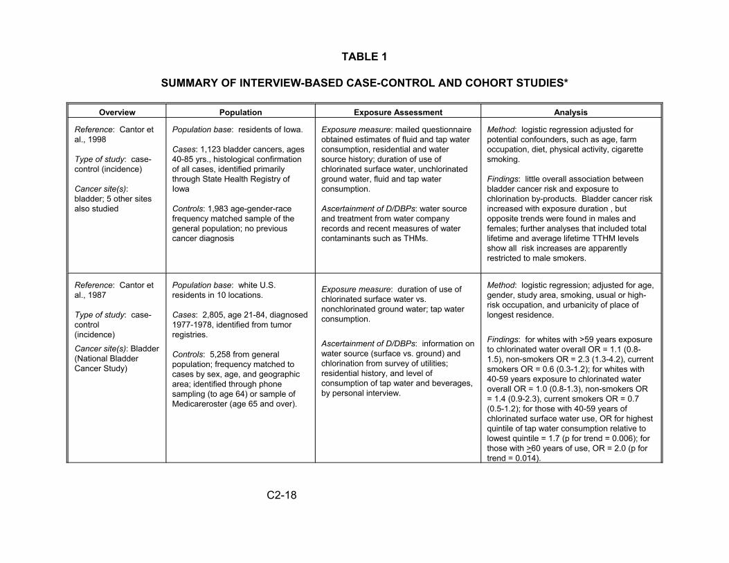
TABLE 1
SUMMARY OF INTERVIEW-BASED CASE-CONTROL AND COHORT STUDIES*
Overview Population Exposure Assessment Analysis
Reference: Cantor et al., 1998
Type of study: case-control (incidence)
Cancer site(s): bladder; 5 other sites also studied
Population base: residents of Iowa.
Cases: 1,123 bladder cancers, ages 40-85 yrs., histological confirmation of all cases, identified primarily through State Health Registry of Iowa
Controls: 1,983 age-gender-race frequency matched sample of the general population; no previous cancer diagnosis
Exposure measure: mailed questionnaire obtained estimates of fluid and tap water consumption, residential and water source history; duration of use of chlorinated surface water, unchlorinated ground water, fluid and tap water consumption.
Ascertainment of D/DBPs: water source and treatment from water company records and recent measures of water contaminants such as THMs.
Method: logistic regression adjusted for potential confounders, such as age, farm occupation, diet, physical activity, cigarette smoking.
Findings: little overall association between bladder cancer risk and exposure to chlorination by-products. Bladder cancer risk increased with exposure duration , but opposite trends were found in males and females; further analyses that included total lifetime and average lifetime TTHM levels show all risk increases are apparently restricted to male smokers.
Reference: Cantor et al., 1987
Type of study: case-control (incidence)
Cancer site(s): Bladder (National Bladder Cancer Study)
Population base: white U.S. residents in 10 locations.
Cases: 2,805, age 21-84, diagnosed 1977-1978, identified from tumor registries.
Controls: 5,258 from general population; frequency matched to cases by sex, age, and geographic area; identified through phone sampling (to age 64) or sample of Medicareroster (age 65 and over).
Exposure measure: duration of use of chlorinated surface water vs. nonchlorinated ground water; tap water consumption.
Ascertainment of D/DBPs: information on water source (surface vs. ground) and chlorination from survey of utilities; residential history, and level of consumption of tap water and beverages, by personal interview.
Method: logistic regression; adjusted for age, gender, study area, smoking, usual or high-risk occupation, and urbanicity of place of longest residence.
Findings: for whites with >59 years exposure to chlorinated water overall OR = 1.1 (0.8-1.5), non-smokers OR = 2.3 (1.3-4.2), current smokers OR = 0.6 (0.3-1.2); for whites with 40-59 years exposure to chlorinated water overall OR = 1.0 (0.8-1.3), non-smokers OR = 1.4 (0.9-2.3), current smokers OR = 0.7 (0.5-1.2); for those with 40-59 years of chlorinated surface water use, OR for highest quintile of tap water consumption relative to lowest quintile = 1.7 (p for trend = 0.006); for those with >60 years of use, OR = 2.0 (p for trend = 0.014).
C2-18
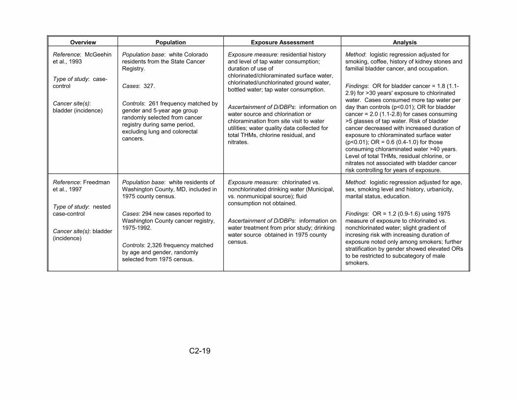
Overview Population Exposure Assessment Analysis
Reference: McGeehin et al., 1993
Type of study: case-control
Cancer site(s): bladder (incidence)
Population base: white Colorado residents from the State Cancer Registry.
Cases: 327.
Controls: 261 frequency matched by gender and 5-year age group randomly selected from cancer registry during same period, excluding lung and colorectal cancers.
Exposure measure: residential history and level of tap water consumption; duration of use of chlorinated/chloraminated surface water, chlorinated/unchlorinated ground water, bottled water; tap water consumption.
Ascertainment of D/DBPs: information on water source and chlorination or chloramination from site visit to water utilities; water quality data collected for total THMs, chlorine residual, and nitrates.
Method: logistic regression adjusted for smoking, coffee, history of kidney stones and familial bladder cancer, and occupation.
Findings: OR for bladder cancer = 1.8 (1.1-2.9) for >30 years' exposure to chlorinated water. Cases consumed more tap water per day than controls (p<0.01); OR for bladder cancer = 2.0 (1.1-2.8) for cases consuming >5 glasses of tap water. Risk of bladder cancer decreased with increased duration of exposure to chloraminated surface water (p<0.01); OR = 0.6 (0.4-1.0) for those consuming chloraminated water >40 years. Level of total THMs, residual chlorine, or nitrates not associated with bladder cancer risk controlling for years of exposure.
Reference: Freedman et al., 1997
Type of study: nested case-control
Cancer site(s): bladder (incidence)
Population base: white residents of Washington County, MD, included in 1975 county census.
Cases: 294 new cases reported to Washington County cancer registry, 1975-1992.
Controls: 2,326 frequency matched by age and gender, randomly selected from 1975 census.
Exposure measure: chlorinated vs. nonchlorinated drinking water (Municipal, vs. nonmunicipal source); fluid consumption not obtained.
Ascertainment of D/DBPs: information on water treatment from prior study; drinking water source obtained in 1975 county census.
Method: logistic regression adjusted for age, sex, smoking level and history, urbanicity, marital status, education.
Findings: OR = 1.2 (0.9-1.6) using 1975 measure of exposure to chlorinated vs. nonchlorinated water; slight gradient of incresing risk with increasing duration of exposure noted only among smokers; further stratification by gender showed elevated ORs to be restricted to subcategory of male smokers.
C2-19
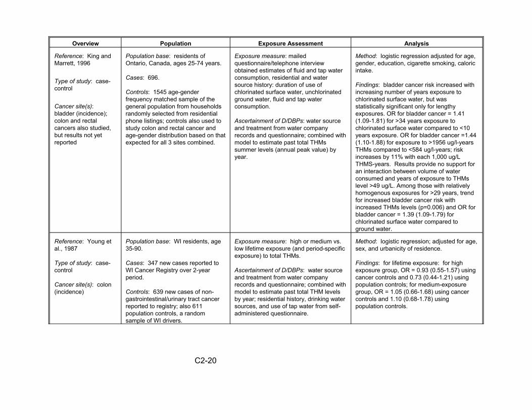
Overview Population Exposure Assessment Analysis
Reference: King and Marrett, 1996
Type of study: case-control
Cancer site(s): bladder (incidence); colon and rectal cancers also studied, but results not yet reported
Population base: residents of Ontario, Canada, ages 25-74 years.
Cases: 696.
Controls: 1545 age-gender frequency matched sample of the general population from households randomly selected from residential phone listings; controls also used to study colon and rectal cancer and age-gender distribution based on that expected for all 3 sites combined.
Exposure measure: mailed questionnaire/telephone interview obtained estimates of fluid and tap water consumption, residential and water source history: duration of use of chlorinated surface water, unchlorinated ground water, fluid and tap water consumption.
Ascertainment of D/DBPs: water source and treatment from water company records and questionnaire; combined with model to estimate past total THMs summer levels (annual peak value) by year.
Method: logistic regression adjusted for age, gender, education, cigarette smoking, caloric intake.
Findings: bladder cancer risk increased with increasing number of years exposure to chlorinated surface water, but was statistically significant only for lengthy exposures. OR for bladder cancer = 1.41 (1.09-1.81) for >34 years exposure to chlorinated surface water compared to <10 years exposure. OR for bladder cancer =1.44 (1.10-1.88) for exposure to >1956 ug/l-years THMs compared to <584 ug/l-years; risk increases by 11% with each 1,000 ug/L THMS-years. Results provide no support for an interaction between volume of water consumed and years of exposure to THMs level >49 ug/L. Among those with relatively homogenous exposures for >29 years, trend for increased bladder cancer risk with increased THMs levels (p=0.006) and OR for bladder cancer = 1.39 (1.09-1.79) for chlorinated surface water compared to ground water.
Reference: Young et al., 1987
Type of study: case-control
Cancer site(s): colon (incidence)
Population base: WI residents, age 35-90.
Cases: 347 new cases reported to WI Cancer Registry over 2-year period.
Controls: 639 new cases of non-gastrointestinal/urinary tract cancer reported to registry; also 611 population controls, a random sample of WI drivers.
Exposure measure: high or medium vs. low lifetime exposure (and period-specific exposure) to total THMs.
Ascertainment of D/DBPs: water source and treatment from water company records and questionnaire; combined with model to estimate past total THM levels by year; residential history, drinking water sources, and use of tap water from self-administered questionnaire.
Method: logistic regression; adjusted for age, sex, and urbanicity of residence.
Findings: for lifetime exposure: for high exposure group, OR = 0.93 (0.55-1.57) using cancer controls and 0.73 (0.44-1.21) using population controls; for medium-exposure group, OR = 1.05 (0.66-1.68) using cancer controls and 1.10 (0.68-1.78) using population controls.
C2-20

Overview Population Exposure Assessment Analysis
Reference: Cragle et al., 1985
Type of study: case-control
Cancer site(s): colon (incidence)
Population base: white NC residents with residency $10 years.
Cases: 200 new cases over 18-month period from 7 NC hospitals, resident in NC $10 years.
Controls: 407 non-cancer hospital patients with admission date nearest diagnosis date of case, matched to case in age, race, gender, vital status, and hospital.
Exposure measure: duration of exposure to chlorinated drinking water (none vs. 1-15 years vs. 16-25 years), 1953-1978.
Ascertainment of D/DBPs: queried local water treatment plants about water source and treatment; residential history by questionnaire (phone or self-administered).
Method: logistic regression adjusted for sex, age, genetic risk, dietary fiber, region of NC, urban residence, smoking, alcohol use, education, and number of pregnancies.
Findings: for age 60: OR = 1.38 (1.10-1.72) for longer exposure and 1.18 (0.94-1.47) for shorter exposure; for age 70: OR = 2.15 (1.70-2.69) and 1.47 (1.16-1.84); for age 80: OR = 3.36 (2.41-4.61) and 1.83 (1.32-2.53).
Reference: Hildesheim, 1998
Type of study: case-control
Cancer site(s): colon and rectal cancers (incidence)
Population base: residents of Iowa
Cases:560 colon cancers, 537 rectal cancers ages 40-85 yrs., histological confirmation of all cases, identified primarily through State Health Registry of Iowa
Controls: 1983 age-gender-race frequency matched sample of the general population ; no previous cancer diagnosis Cases and controls studies had at leasts70% of lifetime drinking water exposures documented
Exposure measure: mailed questionnaire obtained estimates of fluid and tap water consumption, residential and water source history; duration of use of chlorinated surface water, unchlorinated ground water, fluid and tap water consumption.
Ascertainment of D/DBPs: water source and treatment from water company records and recent measures of water contaminants such as THMs.
Method: logistic regression adjusted for potential confounders, such as age, farm occupation, diet, physical activity, cigarette smoking, urbanicity.
Findings: No association between colon cancer and estimates of past chlorination by-product exposure. Rectal cancer risk increased siginificantly with duration of exposure to chlorinated surface water and increasing lifetime THMs exposure; larger odds ratios found among those with low fiber intake and low levels of physical activity.
C2-21
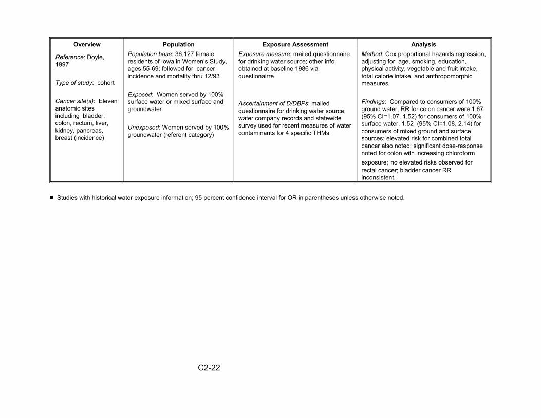
Overview
Reference: Doyle, 1997
Type of study: cohort
Cancer site(s): Eleven anatomic sites including bladder, colon, rectum, liver, kidney, pancreas, breast (incidence)
Population Population base: 36,127 female residents of Iowa in Women’s Study, ages 55-69; followed for cancer incidence and mortality thru 12/93
Exposed: Women served by 100% surface water or mixed surface and groundwater
Unexposed: Women served by 100% groundwater (referent category)
Exposure Assessment Exposure measure: mailed questionnaire for drinking water source; other info obtained at baseline 1986 via questionairre
Ascertainment of D/DBPs: mailed questionnaire for drinking water source; water company records and statewide survey used for recent measures of water contaminants for 4 specific THMs
Analysis Method: Cox proportional hazards regression, adjusting for age, smoking, education, physical activity, vegetable and fruit intake, total calorie intake, and anthropomorphic measures.
Findings: Compared to consumers of 100% ground water, RR for colon cancer were 1.67 (95% CI=1.07, 1.52) for consumers of 100% surface water, 1.52 (95% CI=1.08, 2.14) for consumers of mixed ground and surface sources; elevated risk for combined total cancer also noted; significant dose-response noted for colon with increasing chloroform exposure; no elevated risks observed for rectal cancer; bladder cancer RR inconsistent.
# Studies with historical water exposure information; 95 percent confidence interval for OR in parentheses unless otherwise noted.
C2-22
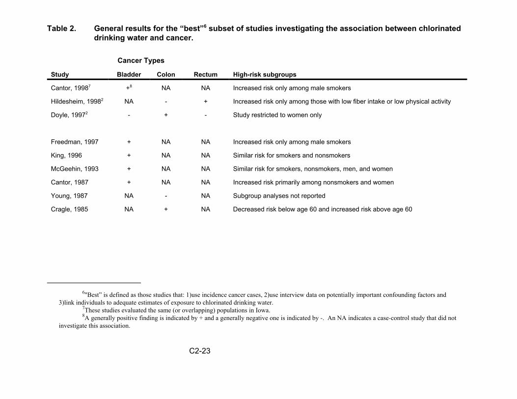
Table 2. General results for the “best”6 subset of studies investigating the association between chlorinated drinking water and cancer.
Cancer Types
Study Bladder Colon Rectum High-risk subgroups
Cantor, 19987 +8 NA NA Increased risk only among male smokers
Hildesheim, 19982 NA - + Increased risk only among those with low fiber intake or low physical activity
Doyle, 19972 - + - Study restricted to women only
Freedman, 1997 + NA NA Increased risk only among male smokers
King, 1996 + NA NA Similar risk for smokers and nonsmokers
McGeehin, 1993 + NA NA Similar risk for smokers, nonsmokers, men, and women
Cantor, 1987 + NA NA Increased risk primarily among nonsmokers and women
Young, 1987 NA - NA Subgroup analyses not reported
Cragle, 1985 NA + NA Decreased risk below age 60 and increased risk above age 60
6"Best” is defined as those studies that: 1)use incidence cancer cases, 2)use interview data on potentially important confounding factors and 3)link individuals to adequate estimates of exposure to chlorinated drinking water.
7These studies evaluated the same (or overlapping) populations in Iowa.8A generally positive finding is indicated by + and a generally negative one is indicated by -. An NA indicates a case-control study that did not
investigate this association.
C2-23
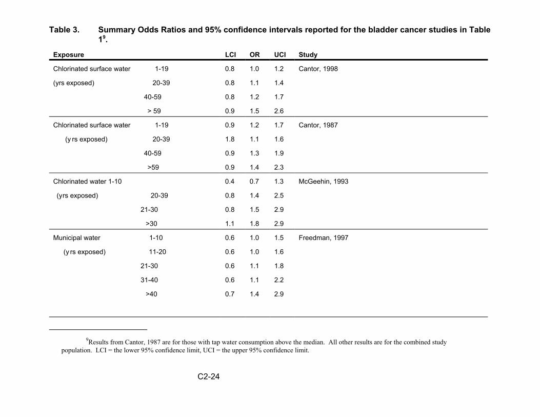
Table 3. Summary Odds Ratios and 95% confidence intervals reported for the bladder cancer studies in Table 19.
Exposure LCI OR UCI Study
Chlorinated surface water 1-19 0.8 1.0 1.2 Cantor, 1998
(yrs exposed) 20-39 0.8 1.1 1.4
40-59 0.8 1.2 1.7
> 59 0.9 1.5 2.6
Chlorinated surface water 1-19 0.9 1.2 1.7 Cantor, 1987
(y rs exposed) 20-39 1.8 1.1 1.6
40-59 0.9 1.3 1.9
>59 0.9 1.4 2.3
Chlorinated water 1-10 0.4 0.7 1.3 McGeehin, 1993
(yrs exposed) 20-39 0.8 1.4 2.5
21-30 0.8 1.5 2.9
>30 1.1 1.8 2.9
Municipal water
(y rs exposed)
1-10 0.6 1.0 1.5
11-20 0.6 1.0 1.6
21-30 0.6 1.1 1.8
31-40 0.6 1.1 2.2
>40 0.7 1.4 2.9
Freedman, 1997
9Results from Cantor, 1987 are for those with tap water consumption above the median. All other results are for the combined study population. LCI = the lower 95% confidence limit, UCI = the upper 95% confidence limit.
C2-24

Exposure LCI OR UCI Study
Chlorinated surface water 10-19 0.7 1.0 1.5 King, 1996
(yrs exposed) 20-34 0.9 1.2 1.5
>34 1.1 1.4 1.8
Chloroform level 1 - 2 0.4 0.9 2.0 Doyle, 1997
(ug/l) 3 - 13 0.6 1.2 2.7
14 - 287 0.3 0.6 1.6
C2-25
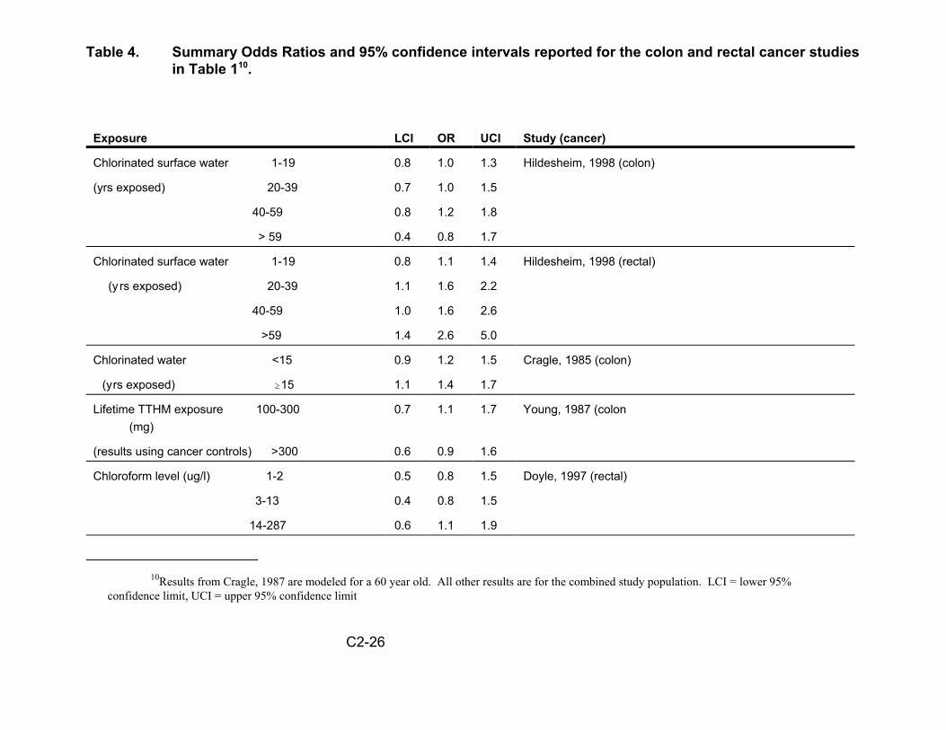
Table 4. Summary Odds Ratios and 95% confidence intervals reported for the colon and rectal cancer studies in Table 110 .
Exposure
Chlorinated surface water
(yrs exposed)
LCI OR UCI
1-19 0.8 1.0 1.3
20-39 0.7 1.0 1.5
40-59 0.8 1.2 1.8
> 59 0.4 0.8 1.7
Study (cancer)
Hildesheim, 1998 (colon)
Chlorinated surface water 1-19 0.8 1.1 1.4 Hildesheim, 1998 (rectal)
(y rs exposed) 20-39 1.1 1.6 2.2
40-59 1.0 1.6 2.6
>59 1.4 2.6 5.0
Chlorinated water <15 0.9 1.2 1.5 Cragle, 1985 (colon)
(yrs exposed) $15 1.1 1.4 1.7
Lifetime TTHM exposure 100-300 (mg)
0.7 1.1 1.7 Young, 1987 (colon
(results using cancer controls) >300 0.6 0.9 1.6
Chloroform level (ug/l) 1-2 0.5 0.8 1.5 Doyle, 1997 (rectal)
3-13 0.4 0.8 1.5
14-287 0.6 1.1 1.9
10Results from Cragle, 1987 are modeled for a 60 year old. All other results are for the combined study population. LCI = lower 95% confidence limit, UCI = upper 95% confidence limit
C2-26
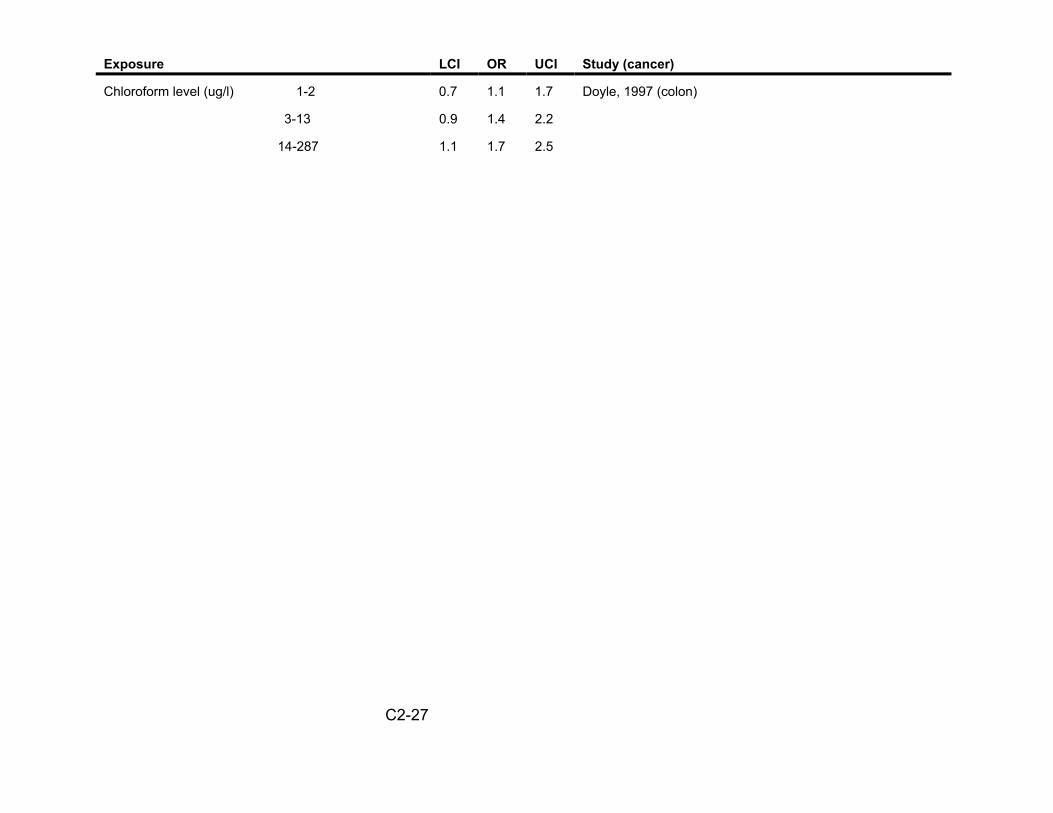
Exposure LCI OR UCI Study (cancer)
Chloroform level (ug/l) 1-2 0.7 1.1 1.7 Doyle, 1997 (colon)
3-13 0.9 1.4 2.2
14-287 1.1 1.7 2.5
C2-27

Table 5. PAR estimates for different assumptions of excess bladder cancer risk.
Suggested OR for Population Estimated annual Estimated sensitivity analysis
Attributable Risk (PAR)11
number of cancers eliminated
national excess cancer rate12
nationally
1.00 0 0 0
1.10 5% 2400 1 EE-5
1.20 10% 4700 2 EE-5
1.30 14% 6600 3 EE-5
1.40 18% 8500 3.5 EE-5
1.50 21% 9900 4 EE-5
Animal data13 0.002% 1 4 EE-9
11PAR= Pe(OR-1)/(1+Pe(OR-1)), where Pe is assumed to be 0.5412Assuming a national population of 250,000,00013Animal data suggests an OR of < 1.00002
C2-28

Appendix II
Draft Peer Review Workshop ReportPeer Review of the “Research Report: The Risk Assessment of Mixtures of
Disinfection Byproducts (DBPs) for Drinking Water Treatment Systems”June 20-12, 2000
Draft Peer Review Workshop ReportPeer Review of the “Research Report: TheRisk Assessment of Mixtures of Disinfection
Byproducts (DBPs) for Drinking WaterTreatment Systems” June 20-21, 2000
National Center for Environmental AssessmentU.S. Environmental Protection Agency
Cincinnati, OH 45268
Prepared byVersar Inc.
6850 Versar CenterSpringfield, VA 22151
July 19, 2000
TABLE OF CONTENTSPAGE
1. INTRODUCTION . . . . . . . . . . . . . . . . . . . . . . . . . . . . . . . . . . . . . . . . . . . . . . . . . . . 1
1.1 Background . . . . . . . . . . . . . . . . . . . . . . . . . . . . . . . . . . . . . . . . . . . . . . . . . . . 11.2 Purpose . . . . . . . . . . . . . . . . . . . . . . . . . . . . . . . . . . . . . . . . . . . . . . . . . . . . . . 2
2. CHARGE TO THE PEER REVIEWERS . . . . . . . . . . . . . . . . . . . . . . . . . . . . . . . . . 3
2.1 Specific Charge Questions . . . . . . . . . . . . . . . . . . . . . . . . . . . . . . . . . . . . . . . . 32.2 Workshop Agenda . . . . . . . . . . . . . . . . . . . . . . . . . . . . . . . . . . . . . . . . . . . . . . 5
3. COMMENTS IN RESPONSE TO EPA CHARGE . . . . . . . . . . . . . . . . . . . . . . . . . . 7
3.1 Q 8 - Overall Evaluation (All Sections DBP Report) . . . . . . . . . . . . . . . . . . . . . 83.2 Q 1 - Introduction and Current State of Science (Section 1&2 DBP Report) . . 9
3.2.1 Introduction (Section 1 DBP Report) . . . . . . . . . . . . . . . . . . . . . . . . . . . . 93.2.2 Current State of the Science (Section 2 DBP Report) . . . . . . . . . . . . . . 10
3.3 Overall Section 3 (Section 3.1-3.7 DBP Report) . . . . . . . . . . . . . . . . . . . . . . . 14
3.3.1 Q 4-Epidemiological & Toxicologic Data (Section 3.1 DBP Report) . . . . 153.3.2 Q 2- Exposure Characterization (Section 3.2 DBP Report) . . . . . . . . . . 173.3.3 Q 3-Unidentified DBPs (Section 3.3 DBP Report) . . . . . . . . . . . . . . . . . 203.3.4 Q 2-Developmental & Reproductive Effects (Section 3.4 DBP Report) . 223.3.5 Q 2-Risk Assessment of Carcinogenic Effects (Section 3.5 DBP Report) 233.3.6 Q 2-Uncertainty & Variability (Section 3.6 DBP Report) . . . . . . . . . . . . . 243.3.7 Q 2-Mixtures Risk Characterization Methods (Section 3.7 DBP Report) 26
3.4 Q 5 - Cumulative Risk Assessment (Section 4 DBP Report) . . . . . . . . . . . . . 273.5 Q 6 - Future Research Needs (Section 5 DBP Report) . . . . . . . . . . . . . . . . . 29
3.5.1 Methods Research (Section 5.1 DBP Report) . . . . . . . . . . . . . . . . . . . . 293.5.2 Cumulative Relative Potency Factor (Section 5.2 DBP Report) . . . . . . . 303.5.3 Epidemiology Research (Section 5.3 DBP Report) . . . . . . . . . . . . . . . . 303.5.4 Development of Toxicologic Data (Section 5.4 DBP Report) . . . . . . . . . 313.5.5 New Section Addition (Section 5.5 DBP Report) . . . . . . . . . . . . . . . . . . 31
3.6 Q 7 - New Data (Overall DBP Report) . . . . . . . . . . . . . . . . . . . . . . . . . . . . . . 32

1. INTRODUCTION
The purpose of this document is to present a preliminary summary of a peer review workshop that was held on June 20 - 21, 2000 in Cincinnati, OH, to peer review the Research Report: The Risk Assessment of Mixtures of Disinfection Byproducts (DBPs) for Drinking Water Treatment Systems. The primary objective of this workshop was to obtain the input of 7 peer reviewers on the scientific and technical aspects of the DBP document.
1.1. BACKGROUND
The U.S. Environmental Protection Agency's (EPA) Office of Research and Development (ORD), National Center for Environmental Assessment - Cincinnati Office (NCEA-Cin) has developed a report that contains information concerning the conduct of risk assessments for mixtures of disinfection by-products (DBPs) across various drinking water treatment systems. Under 42 USC § 300 of the Safe Drinking Water Act Amendments of 1996, it is stated that the Agency will “develop new approaches to the study of complex mixtures, such as mixtures found in drinking water...” This report reflects the current results relative to research in this area over the past five years. It presents: an illustrative DBP mixtures risk characterization; the summary of an expert scientific workshop on this subject; EPA conclusions and recommendations subsequent to the workshop; a conceptual cumulative risk approach; and ideas on future research needs.
The approach to this effort has resulted in the production of three research reports that are contained in the current document that is being submitted for external peer review. Appendix I contains an initial report that was generated as a pre-meeting report to an April 1999 workshop on this subject. It is entitled, Workshop Pre-meeting Report: The Risk Assessment of Mixtures of Disinfection By-products (DBPs) for Drinking Water Treatment Systems (U.S. EPA, 1999a) and was developed to detail the response addition approach to estimating DBP mixture risk that has been developed by NCEA-Cin. Having performed this initial assessment, NCEA-Cin scientists recognized a number of areas for improvement and held the workshop in April 1999 to examine the current method, present ideas to advance the approach, and come to some conclusions relative to new research and development directions. The resulting workshop report is presented in the document as Report 2, entitled, Workshop Report: The Risk Assessment of Mixtures of Disinfection By-products (DBPs) for Drinking Water Treatment Systems. Finally, EPA scientists have used the information from the April 1999 workshop to develop a number of conclusions and recommendations relative to this area of research and to develop a conceptual approach to performing a cumulative risk assessment. This information is presented in the document as Report 1, entitled, EPA Conclusions and Conceptual Approach for the Risk Assessment of Mixtures of Disinfection By-products (DBPs) for Drinking Water Treatment Systems.
1
1.2. PURPOSE
The objective of this Task Order was to coordinate the external peer review of the Research Report: The Risk Assessment of Mixtures of Disinfection Byproducts (DBPs) for Drinking Water Treatment Systems. The document was reviewed by seven experts selected by Versar because of their specific experience in drinking water treatment engineering, chemistry, risk assessment, toxicology, epidemiology, statistical modeling/uncertainty analysis, and exposure assessment. The seven peer reviewers are listed below:
1.2. Mr. Phillipe Daniel, CDM - Drinking water treatment engineering and chemistry. 1.3. Dr. Lynne Haber, TERA - Carcinogenicity, developmental/reproductive toxicity, and
mixtures risk assessment methodology. 1.4. Dr. Jay Nuckols, Colorado State University - Epidemiology, exposure modeling, and
drinking water treatment engineering/chemistry. 1.5. Dr. Shesh Rai, St. Jude Children’s Hospital - Statistical modeling/uncertainty
analysis and epidemiology. 1.6. Dr. Venkat Rao, DynCorp - Carcinogenicity, developmental/reproductive toxicity,
and mixtures risk assessment methodology. 1.7. Dr. John Reif, Colorado State University - Epidemiology. 1.8. Dr. Charles Wilkes, Wilkes Technologies - Exposure modeling, statistical
modeling/uncertainty analysis.
This document details the comments provided at the 2-day workshop held in Cincinnati, OH on June 20 - 21, 2000. The sections that follow are organized according to the charge questions and/or the chapters of the report.
2
2. CHARGE TO THE PEER REVIEWERS AND WORKSHOP AGENDA
This section presents the charge questions posed to the peer reviewers in 2.1 and the workshop agenda in 2.2.
2.1. EPA’S CHARGE MEMO AND QUESTIONS
The external review of this document has the primary goal of evaluating Report 1 on EPA’s conclusions and conceptual approach. This is the portion of the document that can and will be changed based on what the reviewers discuss and recommend. This report requires careful review for accuracy and soundness of conclusions. Both the pre-meeting report (Appendix I) and Report 2 are final documents that cannot be changed, but are included to provide background information and detailed descriptions of the data and methods either used by EPA or proposed during the workshop. In addition to critiquing Report 1, the peer reviewers are also invited to comment on the data, methods and discussions presented in the entire document or to add text on new information and perspectives that are not covered by the document. The summary report of the external review comments generated by this contractual review will be added as Appendix II of the document prior to its final clearance.
EPA recognizes that review of this document requires a multi-disciplinary panel of scientists. EPA expects the peer reviewers to focus their comments on sections of the document that discuss material relative to their areas of expertise, but also to comment on the overall methodology and approaches to the risk assessment to the best of their abilities. For a quick overview of the scientific questions, it is suggested that the peer reviewers read over the charge to the April 1999 workshop participants (introductory material to Report 2). EPA expects the reviewers to have read the document prior to attending the meeting and to come prepared to discuss its scientific strengths and weaknesses. EPA scientists are not planning to make presentations of the material in the document, but will be in attendance at the meeting to clarify and answer questions. The peer review panel is required to write an initial draft peer review report that is due to EPA by the end of the 2nd day of the meeting.
Q 1. Is the introductory material in sections 1 and 2 of Report 1 clearly and concisely written, so that the DBP mixtures problem is well defined, the logic behind approaching this as a mixtures risk assessment is sound, and the current state of the science is understandable and correct?
Q 2. In section 3 of Report 1, has EPA identified the most important issues to work on and resolve under these seven research areas (sections 3.1-3.7, with background information in Report 2)? Specifically address issues related to concentration data, exposure estimates, dose-response information for both cancer and noncancer
3
effects, treatment of unidentified DBPs, choices among mixtures risk characterization methods, and handling of uncertainty and variability.
Q 3. Should the toxicity of unidentified DBPs or of identified DBPs for which little or no data exist be incorporated into the risk assessment? If so, what are the most scientifically appropriate ways to estimate the potential health risks?
Q 4. How can EPA integrate both epidemiologic and toxicologic data into the risk assessment? Are the expert judgment methods discussed in the document (section 3.1. of Report 1 and discussions in Report 2) an appropriate way to incorporate data from each of these disciplines?
Q 5. Given the information in section 3 of Report 1, is the conceptual model for the cumulative risk assessment, shown in section 4 of Report 1, a scientifically sound approach to the DBP mixtures problem? Are there better alternatives to this approach? Are important considerations missing, inaccurately portrayed, or not fully developed?
Q 6. Are the areas of research specified in section 5 of Report 1 as future research directions clearly stated, appropriate as next steps and complete? Should anything be added or deleted?
Q 7. Do the reviewers know of any newer data or methods that EPA has not considered, but should be aware of in order to improve this risk assessment? Specifically address advancements in dose-response modeling, analytical chemistry, exposure characterization, mixtures risk assessment methods, probabilistic techniques, quantitative structure activity relationships, and methods for estimating risk for the unidentified DBPs.
Q 8. What is the reviewers’ overall evaluation of the scientific content, readability and utility of the entire document? Are there suggestions relative to structure or content that would improve the quality of the document?
4
2.2. WORKSHOP AGENDA
Peer Review of Research Report: Risk Assessment of Mixtures of Disinfection By-Products (DBPs) for Drinking Water Treatment Systems
June 20-21, 2000
June 20, 2000 Tuesday
8:00-8:30 Registration/Check In
8:30-8:40 Welcome Terry Harvey, U.S. EPA/NCEA
8:40-8:50 Welcome, Meeting Structure, Objectives, Introduction of Panel David Bottimore, Versar, Inc.
8:50-9:10 Background on the Document: Etiology, Purpose, Approach Linda Teuschler, EPA/NCEA-Cin
9:10-9:20 Overview of the Charge David Bottimore, Versar, Inc.
9:20-10:30 Initial Overall Assessment of the Document; Major Points for Consideration During the Peer Review Meeting
Discussion Leader: David Bottimore Expert Panel Members (5-10 minute summaries from each person)
Q 8. What is the reviewers’ overall evaluation of the scientific content, readability and utility of the entire document? Are there suggestions relative to structure or content that would improve the quality of the document?
10:30-10:45 Break
10:45-11:45 Chapters 1 and 2 - Introduction and Current State of the Science Discussion Leader: Phillipe Daniel
Q 2. In section 3 of Report 1, has EPA identified the most important issues to work on and resolve under these seven research areas (sections 3.1-3.7, with background information in Report 2)? Specifically address issues related to concentration data, exposure estimates, dose-response information for both cancer and noncancer effects, treatment of unidentified DBPs, choices among mixtures risk characterization methods, and handling of uncertainty and variability.
5
Discussion Leaders: Charles Wilkes and Jay Nuckols
Q 3. Should the toxicity of unidentified DBPs or of identified DBPs for which little or no data exist be incorporated into the risk assessment? If so, what are the most scientifically appropriate ways to estimate the potential health risks?
Discussion Leader: Venkat Rao
Q 4. How can EPA integrate both epidemiologic and toxicologic data into the risk assessment? Are the expert judgment methods discussed in the document (section 3.1. of Report 1 and discussions in Report 2) an appropriate way to incorporate data from each of these disciplines?
Discussion Leader: John Reif
2:45-3:00 Break
3:00-4:00 Chapter 4 - Conceptual Model for a Cumulative Risk Approach Discussion Leader: Lynne Haber
Q 6. Are the areas of research specified in section 5 of Report 1 as future research directions clearly stated, appropriate as next steps and complete? Should anything be added or deleted?
Q 7. Do the reviewers know of any newer data or methods that EPA has not considered, but should be aware of in order to improve this risk assessment? Specifically address advancements in dose-response modeling, analytical chemistry, exposure characterization, mixtures risk assessment methods, probabilistic techniques, quantitative structure activity relationships, and methods for estimating risk for the unidentified DBPs.
5:00-5:30 Summation of Issues; Plans for Report Writing David Bottimore, Versar, Inc.
June 21, 2000 Wednesday
8:30-12:00 Final Discussions by the Expert Panel; Development of Recommendations for Revisions
Facilitator: David Bottimore, Versar, Inc.
1:00-5:00 Report Writing; Preliminary Draft of Peer Review Workshop Report - due to EPA by Close of Business
6
3. COMMENTS IN RESPONSE TO EPA CHARGE
This section presents detailed comments that were presented at the peer review workshop. In general, the reviewers felt that the report was well done and that with moderate revisions, it is suitable for publication. In addition, many suggestions were provided on how to make the report more complete and useful for readers. Particularly, almost all the reviewers felt that the document needs a clearly stated purpose and scope. Several individuals suggested minor reorganization of the report to present certain information in a less fragmented manner.
This section is organized according to the charge questions and/or the chapters of the report. Specifically, while most of this section is organized according to the 8 charge questions presented previously, some of the discussion at the workshop deviated from the charge questions and, instead, focused on providing comments according to the report chapters and subsections (Table 3-1). The reviewers recognized the sometimes overlapping nature of the questions and chose (especially for Chapter 3 of the report) to organize the discussion and comments in this manner. Therefore, the following subsections are presented in the following manner:
Table 3-1. Crosswalk of Report Sections, Charge Questions, and Sections of the DBP Report
Section of This Report
3.1
3.2
3.2.1
3.2.2
3.3
3.3.1
3.3.2
3.3.3
3.3.4
3.3.5
3.3.6
3.3.7
3.4
3.5
3.6
Charge Question No.
8
1
1
1
2
4
2 & 4
3
2
2
2
2
5
6
7
Section of DBP Report # 1
All
1 & 2
1
2
All of Section 3
3.1
3.2
3.3
3.4
3.5
3.6
3.7
4
5
All
7
Subsections present comments and suggestions in the following format (1) summary, (2) organizational comments, (3) content comments, and (4) specific comments.
3.1. Q8 - OVERALL EVALUATION (ALL SECTIONS DBP REPORT)
Q8. What is the reviewers’ overall evaluation of the scientific content, readability and utility of the entire document? Are there suggestions relative to structure or content that would improve the quality of the document?
Summary: In response to Question 8, there was a nearly unanimous call for clarification on the purpose of the report and for more information on the context in which the document fits. Similarly, clarification is needed on the scope of the Report 1 document and its relationship to the appendices. Overall, there was general agreement that a cumulative risk assessment approach is an appropriate method for addressing this issue. However, many reviewers believed that further analyses and presentation of the epidemiological, toxicological, and exposure data are needed so the approach is based on the “state of the science.” Of particular note was the call for an expand discussion of exposure assessment, such as the need to account for the variety of DBP mixtures that are likely to be found nationwide. With these changes and some editing (e.g., minor changes to the organization and wording of certain sections) the document would be a helpful tool for directing future work in this area.
Organization Comments: Considerable discussion addressed the organization and outline for the document, particularly with respect to the relationship between the report and the appendices. For the most part the reviewers agreed with the current organization, however suggestions were made on select sections. In a few cases, the case was made to either pull text up from the appendices or to move detailed discussions back to an appendix so as not to interrupt the flow of the report.
Content Comments: In response to Question 8, there was a nearly unanimous call for clarification on the purpose/scope of the report and for more information on the context in which the document fits. The reviewers felt that the document addresses very important and complex issues, but that it needs to be revised in a manner that provides a better picture of the role of the report (and associated efforts) in EPA’s vision for the future. Included in the suggestion was the need for clarification on the relationship of the Report 1 document to the appendices and the possible need to “pull up” some of the details from the appendices to flesh out the technical aspects of the document. One reviewer suggested that the document be reorganized to follow a risk management/decision making paradigm that might more directly influence current rulemaking efforts and regulatory decision-making.
Overall, there was general agreement that a cumulative risk assessment approach, using the response addition and relative potency factor approach, is an appropriate method for addressing this issue. However, many reviewers believed that improved analysis and
8
presentation of the epidemiological, toxicological, and exposure data are needed so the approach is based on the “state of the science.” Included in these suggestions was the recommendation that some of the wording of the epidemiology sections be edited and that discussion be clarified. For example, discussion addressed the need for new epidemiology studies to evaluate effects in the context of specific DBPs of interest (e.g., brominated compounds). There was discussion about effects of DBPs for endpoints (e.g., liver and kidney effects) that may not have been identified to date by epidemiology.
Several reviewers commented that EPA should expand the discussion of exposure assessment. Included here is the need for the risk assessment to account for the variety of DBP mixtures that are likely to be found nationwide. Better data are needed on DBPs in drinking water at the tap to incorporate into the assessment. Furthermore, the reviewers stated that the risk assessment approach should account for the formation of brominated and mixed chloro-/bromo- compounds when different technologies and different source water characteristics are considered. The reviewers also stated the need to include inhalation and dermal exposure routes into the risk assessment. Accordingly, more extensive toxicity data for the effects of these chemicals via these exposure routes will be needed in the future. Comments called for sensitivity analyses to be performed on the risk assessment approach to determine those parameters that may be the most important risk drivers. From this analysis, priorities can be set on those issues that will have the greatest impact on the risk.
Several reviewers commented that the document could use a thorough editing. Furthermore the organization and wording of certain sections of the document should be improved. More detailed recommendations follow below.
3.2. Q1 - INTRODUCTION AND CURRENT STATE OF THE SCIENCE (SECTIONS 1 AND 2 DBP REPORT)
Q1. Is the introductory material in sections 1 and 2 of Report 1 clearly and concisely written, so that the DBP mixtures problem is well defined, the logic behind approaching this as a mixtures risk assessment is sound, and the current state of the science is understandable and correct?
3.2.1. Introduction (Section 1 DBP Report).
Summary: This section of the document needs significant revision to more concisely present the problem and outline the scope of this document.
Organization Comments: Significant changes in Section 1 of the report are advised. A revised outline would include:
1. Drinking water: sources, treatments, distribution systems à mixtures of compounds (DBPs) of potential health significance (i.e., consequence of low-level risk over large population).
9

2. Regulations: previous, current, future. Issues of concern. 3. Relationship between Office of Water and NCEA. 4. Purpose of the report: to guide further development of this effort to support regulatory
decision-making 5. Context of this effort: previous efforts and reports 6. Report overview
Content Comments: Risk management alternatives, principal questions relevant to regulatory decision-making, and the schedule by which specific information can be furnished needs to be added. The reviewers also suggested the following changes. Move epidemiology discussion into Section 2. As presently written, epidemiology discussions are scattered throughout the document (e.g., pages 1-2, 1-5, 1-7, and 1-14). These should be streamlined and combined to provide more cohesive discussion. In addition, the language should be more neutral i.e., not using terms such as used on 1-2 of only relatively weakness, questionable, and entirely dismissed and the discussion more balanced. Further comments on epidemiology are presented under the comments in Section 3.3.1.
Specific Comments:
I. Risk characterization discussion/outline on page 1-1 needs expansion and clarification. II. Alternative hypothesis discussion on page 1-2: #2 is unclear. III. Add the potential for an unidentified constituent being responsible for the response in
epidemiology studies (e.g., could NDMA be such a compound?). IV. The hypothesis of certain vulnerable populations resulting in the observed response
should be noted (e.g., insulin signaling pathway hypothesis with DCA as made by Dr. Richard Bull).
V. Since this is a report on DBPs, the benefits of disinfection do not need to be discussed (or neutrally framed within the compartive risk framework).
3.2.2. Current State of the Science (Section 2 DBP Report).
Summary: Significant changes are advised.
Organization Comments: A revised outline would include:
I. Objective II. Risk paradigm III. Hazard identification and dose response: discussion of endpoints and lines of evidence
a. Cancer S Description S Epidemiology S Animal toxicology S Mechanistic toxicology S In vitro toxicology
10

b. Reproductive/Developmental S Description S Epidemiology S Animal toxicology S Mechanistic toxicology S In vitro toxicology
c. Other S Epidemiology S Animal toxicology S Mechanistic toxicology S In vitro toxicology
d. Impact of exposure routes IV. Exposure assessment V. Risk characterization method
In addition, material that is introduced in Section 2 should be more fully explained at this point rather than repeated and expanded later. For example, information on exposure is introduced in Section 2, but not fully explained until Section 3. The document would probably be clearer and less redundant if this information is presented once, and then Section 3 discusses the outstanding questions. Or consider another example, reproductive/developmental discussion in Section 3.4 should be moved/introduced in Section 2.
Content Comments:
I. Information on toxicology and epidemiology is diffused – it should be consolidated in a concise format and brought up-to-date.
II. Concordance: Clarify what is meant with respect to site, type, and doses. Why should we expect to see concordance? Non-concordance discussion must be far more specific: e.g., site, type, histology, dose. Dose discrepancies are one element. Concordance and non-concordance: limitations of studies? Expected non-concordance?
III. Epidemiology discussion: need better appreciation for nature of environmental epidemiology studies: difficulty of determining causation, the need to view results in the context of other mixture studies. It is not unusual to find low risks from many epidemiology studies.
IV. A preferable epidemiology summary statement is found in Report 2 at 2-1 though this section still needs updating.
V. The issue of consistency of findings in epidemiological studies should be stated accurately. For bladder cancer, there is consistent evidence from interview-based
11

studies that there is an increase in risk associated with long term exposure to chlorinated water. This comes from 5 case control studies and 1 cohort study. There is inconsistency with respect to the sub-populations where the effect is observed; i.e., men and women, smokers and non-smokers. For colon and rectal cancer, the findings are based on fewer studies, and are inconsistent because some studies show an effect an some do not. For the reproductive epidemiology data, there are relatively few studies. Since several individual outcomes are assessed, the database is sparse with respect to specific outcomes; e.g., neural tube defects. Among those studies examining common outcomes (low birth weight, intrauterine growth retardation, developmental defects) the findings are inconsistent. It is not clear how factors such as exposure misclassification and differences in the constituents of the DBP mixture may have affected the results of these studies. It is not clear whether residual confounding, not considered by investigators, could have biased the results.
VI. The single sentence at 1-5, para 2 is accurate but could be expanded to reflect the state of the science by summarizing the evidence for cancer and reproductive outcomes separately. On page 1-14, the findings from the epidemiological studies are discussed briefly and reference is made to Appendix C of Appendix 1. Table 5 of Report 1 is focused only on cancer. There are no summary data provided for human reproductive studies although the toxicological data for reproductive effects is summarized and incorporated into the report (Tables 2 & 3). This is an obvious omission. The results of reproductive studies should be incorporated into a table and the database updated to include recent publications not included in the report or appendices. On page1-14, par. 2, additional references are needed for human studies of reproductive endpoints and are provided below. The statement concerning cancer and odds ratios is incorrect, poorly worded and requires modification.
VII. Table 5 requires revision. The Doyle study (1997) contained only 2 cases of bladder cancer in the exposed group (43 overall). It is highly questionable whether this study should be used to draw any inferences about bladder cancer. Footnote (b) refers to the Iowa studies. The cases in these Iowa studies are independent of each other, defined by site; there is some overlap among controls.
VIII. Exposure assessment discussion should indicate evolution of DBPs from treatment to tap; show how different mixtures result according to source water characteristics, treatment technology, and final disinfectant type. Indicate importance of different human exposure pathways, not just oral.
IX. Need better introduction to Section 2.4.1. Instead of focusing on one option, several alternatives should be described first before the discussion turns to selecting one over the others. For example, discuss additivity, synergism, and antagonism (e.g., use additivity figure) and provide illustration of options (e.g., response addition vs dose addition). The discussion of alternative methods is important. Should the illustrative treatment example drawn from Report 2 be an appendix?
12
Specific Comments:
1. While Table 1 represents the current status of assessments, almost all of the assessments in Table 1 are in the process of being updated by the Office of Water and by ORD, and the document should note that, so that the reader will know to look for updated values. A separate table of current/ongoing assessments of DBPs would be useful. This information could be obtained from the Office of Water.
2. While the formaldehyde result reported in Table 1 is consistent with IRIS, there may be more recent information.
3. Since the purpose of Tables 2 and 3 is unclear and the data are not essential to the argument, it may be advisable to either delete these tables or to move the LOAELs/NOAELs to an appendix. Several reasons why it can be misleading to present this detailed quantitative information include: (a) Except for the NTP (1997) study, all of the HAN studies were conducted using a tricaprylin vehicle, and this vehicle alone can cause increased post-implantation loss and soft tissue malformations (Christ et al., 1995, 1996; Smith et al., 1989a). For example, when TCAN was administered in corn oil, the NOAEL was 35 mg/kg-day and the LOAEL was 55 mg/kg-day for developmental toxicity, based on increased post-implantation loss and a number of types of malformations, in contrast to an AEL of 15 mg-kg-day for TCAN in tricaprylin in the same study (Christ et al., 1996). (As noted in Table 2, 7.5 mg/kg-day was a LOAEL and 1 mg/kg-day was a NOAEL in another study conducted with tricaprylin.) Additional information is in a recent update to the Drinking Water Criteria Document on HANs. (b) It is unclear whether the table is intended to list (all of) the available toxicity data (as stated), or whether only the study identifying the critical effect for each chemical is shown. Additional abstracts and in vitro studies are available, but were not included in this list. If the document authors wish to retain these tables, they should either update the text, just provide qualitative information on reproductive/developmental effects of the HANs and haloacetic acids, or leave it in an appendix with all the appropriate caveats.
4. While standard deviations of IRIS data presented in Tables 1-3 are not readily available, such information would be useful to obtain for uncertainty analysis.
5. It would be useful to supplement Table 6 with information on other DBPs (or classes of DBPs) found in drinking water, to give a sense of what the universe of DBPs is like. DBPs outlined in Table 6 should be expanded to note brominated analogues (and mixed bromochloro species). Reporting the values on a molar basis in the text would also be helpful. Finally, note that Figure 1 is only an example and not representative of all waters or treatment technologies – it is for chlorination and chloramination of a moderate bromide containing water.
13
6. Precursors (pages 1-4 and 1-5): should either refer to inorganic or bromide but not both.
7. In vivo studies of mixtures were limited by concentration effects (i.e., salt limitations) and should be noted (1-5).
8. On page 1-9, line 2: Section 2.3 of Report 2 does not list or refer to the hundreds of potential DBPs. It would be better to Section 3.3 of the current report, which lists DBPs, or refer to specific table(s) in report 2 to give the reader a sense of the range of DBPs. The list of DBPs evaluated by QSAR in Appendix B.3 of the pre-meeting report is also informative for providing the range of DBPs identified beyond those listed in tables 1 and 2 of the main report.
9. The notion of dose additivity for complex mixtures (1-9) has been widely used for low concentration components and should be referenced (i.e., these observations are consistent with other studies and other expert groups).
10. On pages 1-12 and 1-13: It is difficult to compare the studies because of the multiplicity of units used. It would help the reader to report the units used by the authors, and then to report the doses in standardized units.
11. On page 1- 14, lines 4-5: Unclear. Are the words data on missing?
12. In discussing the three factors on 1-17 and 1-19 there was no analysis of which factors were likely to be most important (e.g., is bioavailability refer to fate in treatment and distribution or to likelihood of human metabolism).
13. Response addition methodology (page 1-22) should examine the mixtures associated with the risk management alternatives and scenarios of concern to see which issues are amenable to the proposed analysis.
14. The example (1-23) focused on one water and did not evaluate a final chloramination scenario that would be a likely regulatory alternative.
15. It would be useful to present Figure 2 here, rather than later in the document (page 1-23).
16. Expand discussion to include stochastic characterization of input data.
3.3. OVERALL SECTION 3 (SECTIONS 3.1-3.7 DBP REPORT)
Q2. In section 3 of Report 1, has EPA identified the most important issues to work on and resolve under these seven research areas (sections 3.1-3.7, with background information in Report 2)? Specifically address issues related to concentration data, exposure estimates, dose-response information for both cancer and noncancer effects, treatment of unidentified DBPs, choices among mixtures risk characterization methods, and handling of uncertainty and variability.
14

General Comments: Chapter 3 is a summary of EPA’s priority conclusions and recommendations arising primarily from the April 1999 Workshop. As such, Chapter 3 should be renamed to “EPA’s Major Conclusions and Recommendations based on the April 1999 Workshop.” The introduction to the chapter should include a discussion of the Workshop, and be framed addressing issues and problems raised in the “state of science” discussion from Chapter 2, clearly discussing what EPA accepted, what was rejected, and the reasons. “State of science” information in Chapter 3 should be moved to Chapter 2. The recommendations given in Chapter 3 regarding gathering additional data should be evaluated and prioritized using techniques such as sensitivity analysis. Models and methods recommended in Chapter 3 should be validated where possible.
Structure:
* Use charge questions as format for formulation of report* Move “state of science” information from EPA Workshop report to Chapter 2* Chapter 3: keep as summary of how 1999 workshop was used to formulate
recommendations * Chapter 3 should be framed as addressing issues and problems raised in Chapter
2 being clear what EPA accepted (or not) and why; * Every recommendation should be evaluated (for example, sensitivity analysis) and
prioritized. * Validation of exposure models should be addressed
3.3.1. Q4 - Integration of Epidemiologic and Toxicologic Data (Section 3.1 DBP Report).
Q4. How can EPA integrate both epidemiologic and toxicologic data into the risk assessment? Are the expert judgment methods discussed in the document (section 3.1. of Report 1 and discussions in Report 2) an appropriate way to incorporate data from each of these disciplines?
Summary: The proposed risk assessment will incorporate data from toxicologic studies in laboratory animals and epidemiologic studies of human populations. This section of the report focuses on integrating these two data sources and raises several issues with respect to expert judgement, concordance in findings between animal and human studies, sensitive subpopulations, and meta-analysis.
Organization Comments: The section provides rationale for integrating the epidemiologic and toxicologic data, followed by a series of bullet-form recommendations based on the 1999 workshop. Unlike the remainder of the section, where recommendations for the risk assessment are made directly, the recommendations in 3.1 take the form of recommendations for further research and should be moved to Section 5. Although some recommendations are clearly topics for further research, others are reasonable recommendations for immediate implementation. The bullets should be separated according to this scheme.
15
Content Comments: In this section, and elsewhere in the document, the point is raised that the data from toxicologic studies and epidemiologic studies lack concordance (1-27). This statement requires clarification and further documentation in the report. Concordance between groups of studies can be evaluated at several levels (eg., with respect to organ system involvement, site of lesion, histopathologic characterization or tumor type, and with respect to dose or concentration of xenobiotic required to produce the observed effect). There is concordance between epidemiologic and toxicologic data at several levels. There is evidence of carcinogenicity, effects on reproductive and developmental endpoints, and to some extent, for specific disorders such as urinary tract cancer and fetal growth parameters. There is organ system concordance between findings of kidney cancer in rodents and bladder cancer in humans and between hepatotoxic effects of THMs in animals and of chloroform in case studies and occupational studies in humans. There is concordance between the finding of full litter resorption and evidence of increased risk for spontaneous abortion in human studies (Walker et al., 1998). The lack of concordance may be largely a matter of administered (animal) or estimated (human) dose. The failure to find a given effect at a particular dose across species may reflect several factors as pointed out in the first paragraph on 1-28.
Integration of the epidemiological and toxicological data, at a minimum, requires that the insufficiency and incompleteness of the toxicological approach be recognized. The traditional toxicological approach focuses on individual contaminants thereby falling into the trap EPA’s Science Advisory Board has recently warned against: risk management decisions that focus on the reduction of particular risks rather than on the reduction of total risks (EPASAB, 1999 and 2000 – discussions on Integrated Environmental Decision Making in the 21st Century). That is the burden of this NCEA effort.
The reviewers found that the recommendation to pursue the use of expert judgement in setting bounds for human risk and establishing probabilities for specific risk estimate from published epidemiological studies had merit. The paper by Evans (1994) on bladder cancer risk and long-term consumption of chlorinated water provides an example of the approach. The expert judgement process should be pursued because it may (1) aid in regulatory process, (2) dampen bias, (3) expand the literature database, and help to generate hypotheses and identify knowledge gaps. The caveats are that (1) the proper instrument is selected, and (2) a panel of qualified, unbiased experts can be identified. The approach could be applied to several categories of risk assessment (ie tox-epi data integration, exposure assessment). The publication of additional studies of high quality on this topic provide a dataset that could be used to explore the utility of expert judgement as suggested in the report. Expert judgement could be used to select the appropriate literature base, refine the questions to be asked based on the data available, and identify knowledge gaps in each category of interest. Expert judgedment approaches should include face-to-face discussions so that the benefit of learning from other experts and building from each others’ knowledge base can be realized.
The issue of sensitive subsets of populations of animals and humans should be defined further. As written, this appears to apply to demographic variables such as age, gender and race and their equivalents in rodents. This concept should be kept separate from the issue of susceptibility markers such as genetic polymorphisms (e.g., GST
16

enzymes, acetylation) which should form the basis of an additional research recommendation for integrating human and animal data.
The recommendations concerning meta-analysis should be rephrased to reflect the intent of the authors. It appears from the earlier report that there may be compelling reasons to avoid meta-analysis, or at minimum, to be extremely judicious in potential application of this technique. The panel concurs with this view, and recommends that the recommendations on 1-29 be re-written to reflect EPA’s position. If meta-analysis is recommended as a technique to be used in risk assessment, the framework should be outlined briefly. If meta-analysis is not recommended, the text should be revised accordingly and the recommendation deleted.
Further in the report (3-2), the issue of incorporating biomarkers into human studies is raised. The issue of biomarkers should be included here as a recommendation as well. Identification and validation of suitable biomarkers of exposure and effect would be another important means to integrate epidemiologic and toxicologic data on a dose-response basis.
3.3.2. Q2 - Improvements in Exposure Characterization (Section 3.2 DBP Report).
Q2. In section 3 of Report 1, has EPA identified the most important issues to work on and resolve under these seven research areas (sections 3.1-3.7, with background information in Report 2)? Specifically address issues related to concentration data, exposure estimates, dose-response information for both cancer and noncancer effects, treatment of unidentified DBPs, choices among mixtures risk characterization methods, and handling of uncertainty and variability.
Summary: The exposure characterization methods presented in the report were very general. The description of these methods needs to start with a global description of the current state of exposure assessment techniques, including a discussion of exposure assessment priorities and each method’s strengths and weaknesses. Recognizing that the focus of this document is not on exposure assessment, a judgment needs to be made regarding the level of detail. The authors may wish to include a general review, and cite appropriate technical publications that discuss in greater detail these methods. Depending upon the level of detail the authors choose to address exposure assessment within the document, a fairly detailed discussion of the necessary data, parameter values, and other factors that influence the exposure may be appropriate, including a discussion of the current state of knowledge for the parameter and data needs.
Exposure assessment in the context of risk assessment from DBPs should include characterization of water quality, biomarkers (future research necessary), all potential routes of exposure, and factors related to water-use activity and environment for the study population.
Characterization of Water Quality: The draft report mentions that the range of DBP concentrations are important, but other than treatment practices, does not discuss factors that influence these concentrations. The authors should consider a general overview of the important processes that occur as a result of disinfection, and between the treatment plant and the tap. Possible topics include the characteristics of the water supply, alternative treatment processes, changes in DBP concentrations as it flows through the distribution
17
system, the effect of seasonal variations in water quality and temperature, and the effect of point of use devices (eg, water filters, storage in hot water tanks, etc). Specific comments from the panel on this topic were as follows:
1. Different treatment technologies will create mixtures that are qualitatively and quantitatively different. What is most important is that the DBP we are reasonably sure will be formed by certain technologies are as completely accounted for as possible.
2. The report states that "the range of individual DBP concentrations within the distribution system over the etiological relevant time period" should be incorporated in developing exposure models for risk assessment. Current state of the science demonstrates that each of these variables is mutually exclusive that is, while one may be able to discern individual DBPs for a specific utility at a specific (and narrow, ie maybe seasonal) period of time; it is a daunting task to define this exposure variable over a sufficient geographic region (within a utility or across a set of utilities), and to capture a sufficient study population for the necessary statistical power to differentiate relative risk. This problem is compounded if the etiological time period is a matter of years. Furthermore, current science on this issue has only dealt with THM speciation, and not even began to address the other DBPs identified as potentially toxic by this report).
3. The report states that ICR data should be used to characterize DBP mixture "exposures". ICR is composed of quarterly samples (at best composite over a day, but most likely grab samples) at the Point of Entry from the WTP to the distribution system, and approximately 4 other locations in the distribution system. The dataset is restricted to utilities with a service population greater than 100,000; Therefore, the data set is composed of a sample size of six measurements at each location over an 18 month period in the late 1990's. While the dataset may be very useful from a regulatory standpoint in characterizing DBP occurrence in this subset of large utilities (approximately 250 utilities out of an estimated 60,000 utilities that serve the people of the USA); it does little to assist in defining potential exposure to individuals over a etiological relevant time period for an epidemiological study. The exception might be a retrospective reproductive or developmental epidemiological study design in the service population for one or more of the participating utilities. It is a shame that a prospective study could not have been incorporated into the ICR study plan.
4. The report recommends that "for cancer, annual exposure estimates [based on utility water quality] may be required". I have never understood this logic for exposure reconstruction in cancer epidemiology. Let us assume the most simplest of scenarios, where all participants in an epidemiological study of cancer live at the same location for their entire lives, and the DBP production by their respective water utility was consistent over this time period. Spatial and/or temporal variation in DBP concentrations could result in a significant variation over each annual cycle during the "etiological relevant time period" for some fraction of the study population, depending on the geographic extent of the study. Classifying the population according to the annual average could introduce significant misclassification of exposure if peaks in exposure are relevant to risk. The annual average classifies the population towards the "central tendency", where the tails of exposure
18
distribution across the study population are lost, and exposure classification is toward a mean value. Misclassification of exposure that is nondifferential by disease status biases the risk estimate towards the null, thus true associations between a disease and an exposure may be missed or underestimated.
5. In my opinion, the most important contribution that USEPA could make toward improvements in exposure characterization are missing from this report. That is (1) to work with health scientists in estimating historic levels of DBPs in a specific set of utilities in order that a definitive epidemiological study can be conducted and, perhaps more importantly, (2) to support collection of DBP monitoring data that could be used in a prospective epidemiological study.
6. The exposure characterization necessarily needs to start with an understanding of the DBP concentrations in the water supply. It is likely not sufficient to take measurements at the treatment facility and at system nodes. Rather, the reactions that occur in the system are likely to be important, as they are a function of the duration of time spent in the distribution system, the temperature, the constituents in the water supply, and a variety of other variables. For example, the time the water spends in the water heater and water-use activities that occur after the water sits in the water heater for long periods need to be considered. The DBP concentrations are likely at their highest after extended storage in the water heater, and inhalation exposure to the volatile constituents may be larger than currently predicted. This may also be true of dermal exposure to lesser volatile DBPs.
7. On mixture characterization methods, studying reproducible disinfection scenarios on a range of bromide-TOC matrices should have a high priority.
8. When predictive models are used to reconstruct water quality at the tap (or other unit of analysis in an epi study, ie census block group), validation of models should be addressed.
Biomarkers:
1. The report states that "biomarkers of exposure should be used in future analytical epidemiological studies", and that "it is critical to include all exposure routes". While the researchers that have been doing this work may agree, the report would be much stronger if it made specific recommendations as to how to achieve these objectives, rather than broad brush statements of needs, which we are all aware of already.
2. The incorporation of biomarkers of exposure, susceptibility and effect into epidemiological studies should be added in the list of research recommendations
3. Use of biomarkers as endpoints [in epidemiological studies] could be coordinated with similar studies in animals for risk assessment purposes .
Route of exposure:
1. Despite the sentence on 1-28, para 1 regarding differences in metabolism of DBPs that are ingested and inhaled or dermally absorbed, the issue of route of exposure
19
was not treated satisfactorily in earlier accompanying work. The risk characterization reported in Appendix 1 relied on a single exposure pathway. EPA must resolve the issue of multiple routes of exposure to volatile DBP in further risk assessment work for the findings to be credible.
2. The recommendation to account for multi-route exposures when doing DBP risk assessment (1-30) is appropriate.
3. Research topics should include the development of pharmacokinetic models to be used to evaluate route-specific uptake for different classes of DBPs and related issues.
4. The issues of exposure pathways and route specific exposure were not adequately addressed. While mentioning the other routes, the risk characterization dealt only with the ingestion route. The inhalation and dermal routes have been shown to be important by several publications (ILSI, Exposure to Contaminants in Drinking Water, Ed Stephen S. Olin, 1998). A discussion on factors influencing each route of exposure should address topics such as route specific factors and chemical volatility.
5. Validation of exposure models should be addressed
Activity patterns / environment:
1. A discussion of the important behavioral and environmental issues affecting exposure should be included. Possible discussion topics include a discussion of water-use behavior, building characteristics, inter-occupant behavior, various water-use devices, and historical exposures.
2. The activities of other family members are known to impact the exposure of a given individual (e.g., when consecutive showers are taken, the second shower is expected to give a substantially larger dose than the first shower). Several technical papers have been written analyzing this impact. However, there are very few studies of family-type activity patterns.
3. There are issues with estimating long-term exposure when chronic endpoints are of concern. Current exposure models deal with exposure under a given set of conditions, but little work has been done to address a population's historical exposures.
4. Validation of exposure models should be addressed
3.3.3. Q3 - Unidentified DBPs (Section 3.3 DBP Report).
Q3. Should the toxicity of unidentified DBPs or of identified DBPs for which little or no data exist be incorporated into the risk assessment? If so, what are the most scientifically appropriate ways to estimate the potential health risks?
20
Summary: External peer review and discussion on the unidentified DBPs may be grouped under the following categories:
Content Comments:
1. Approaches to chemical characterization and classification of DBPs 2. Analytical and modeling techniques to include unidentified DBPs in hazard analysis 3. QSTR as a predictive tool for unidentified QSTR. 4. Summary of the ILSI workshop
Specific Comments:
1. Approaches to Classification of DBPs: The peer review group considered theClassification of DBPs in to Group A, B, and C categories as reasonable approach. However, subgrouping of known and identified halogenated DBP (Group A) into Cl- and Br- compounds was suggested as even better from a risk assessment and management point of view. In this regard, more effort in identifying unknown DBPs based on additional analytical studies was considered necessary. No other specific recommendations were made on this topic.
2. Unidentified DBPs: Most of the discussion was focused on the approaches to handling the unidentified halogenated DBPs (Group B). Development of an approach using existing toxicity parameters such as the lethal dose (LD50, LD10, etc.) for known DBPs (Group A) to unknown DBPs (Group B) was suggested by some peer review group members. Studies to develop toxicity parameters for Group B DBPs as a whole may be another option, although there are mechanistic weaknesses in doing so. Some review group members suggested that a review of Group C (non-halogenated DBP) may be necessary at the drinking water consumption level, for it would provide the basis for the type of disinfection and the types and extent of DBPs.
3. QSTR as a Predictive Tool: A number of peer review members were of the opinion that quantitative structure toxicity relationship (QSTR) is perhaps best suited in to predict toxicity of Group B DBPs. Since QSTR is an iterative process evolving through continuo input of new data as a part of the model validation process, targeted tasks for QSTR should be identified to gain from this process. It was also suggested that the QSTR could just be focused on the Cl-, Br- and mixed Cl-/Br
groupings of the DBPs. Use of probabilistic techniques in handling uncertainties associated with unknown DBPs was discussed. In this regard, establishing bounds for the distribution of toxicity values (Group A) for known compounds was suggested as perhaps as the first step.
4. Summary of ILSI Workshop: Review group suggested either moving the ILSI workshop summary to the Appendix or get the information integrated to the document. The format as is reads repetitive and covers topics not related to the section.
21
3.3.4. Q2 - Risk Assessment of Developmental and Reproductive Effects (Section 3.4 DBP Report).
Q2. In section 3 of Report 1, has EPA identified the most important issues to work on and resolve under these seven research areas (sections 3.1-3.7, with background information in Report 2)? Specifically address issues related to concentration data, exposure estimates, dose-response information for both cancer and noncancer effects, treatment of unidentified DBPs, choices among mixtures risk characterization methods, and handling of uncertainty and variability.
Summary: The general approach was considered appropriate and valid, but significant additional explanation of the approach and rationale for the approach is needed.
General comments:
• Additional information needs to be provided, either in this section or earlier in the document, qualitatively walking through the “illustrative example.” This includes discussing the reason for the choice of endpoints, basics of how the modeling was done, and the rationale for key choices made in the calculations. For example, the text should address the potential for other non-cancer effects resulting from exposure to DBPs (including issues of whether the epidemiology studies show that other effects would not be expected, or whether these endpoints have just not been adequately evaluated) and discuss why the document focuses on reproductive/developmental effects. The document should also address the rationale for using no-threshold risk models for reproductive/developmental endpoints (which have traditionally been considered noncancer effects for which a threshold of toxicity exists). This discussion should include both the biological basis for the possible absence of a threshold, and the practical reasons for assuming a threshold.
• The panel did not see a need to link endpoints such as low birth weight to such serous effects as infant mortality.
• Data modeled do not need to be quantalized. A hybrid continuous benchmark dose model (which models continuous data, but expresses the BMD in terms of increased risk) could be used.
• If multiple chemicals act via the same mode of action, the exposure concentration for each individual chemical could be below the threshold for that chemical, but one might expect that an effect could result from exposure to the resulting mixture. The text at the top of page 40 should address this possibility.
Specific Comments:
P. 40, line 2: This should be the exposure concentrations were below the threshold estimate (or threshold above the exposure concentration).
22
3.3.5. Q2 - Risk Assessment of Carcinogenic Effects (Section 3.5 DBP Report).
Q2. In section 3 of Report 1, has EPA identified the most important issues to work on and resolve under these seven research areas (sections 3.1-3.7, with background information in Report 2)? Specifically address issues related to concentration data, exposure estimates, dose-response information for both cancer and noncancer effects, treatment of unidentified DBPs, choices among mixtures risk characterization methods, and handling of uncertainty and variability.
Summary: External peer review and discussion on the carcinogenic risk assessment for DBPs may be grouped under the following categories:
Content Comments:
1. Concordance (or the lack of it) 2. Threshold Issue 3. Mechanistic Information 4. Summary of ILSI Workshop
Specific Comments:
1. Concordance (or the lack of it): The information provided on this topic under this section was considered insufficient by the review team. Differences in concordance of tumor sites could as well be due to differences in the experimental procedures, type of animal used, etc. Lack of concordance in tumor sites may not have anything to do with the more substantial issue on the concordance between experimental and epidemiological evidence. This issue requires clarification.
2. Threshold Issue: Threshold issue stems both from (a) possibility of the presence of threshold and (b) extrapolation (if it is present) to all DBPs. It is unclear if there is a threshold for carcinogenic effects of DBPs (carcinogenic species). A clear determination is first needed before this concept is applied to other DBPs. Some peer review members suggested whether QSTR may have an application on the threshold issue, although such an application is possible only for the known DBPs (Group A) with data on carcinogenicity. No changes were recommended to this section under this chapter.
3. Mechanistic Information: Mechanistic information is a fundamental requirement to develop a robust risk assessment approach. However, it is unclear how this requirement could be met with chemical mixtures. The sentence (page 43) needs modification to better reflect this fundamental shortcoming with mixtures. Note on the epidemiological and statistical modeling should be deleted from this sentence and include separately.
4. Summary of ILSI Workshop: Review group suggested either moving the ILSI workshop summary to the Appendix or get the information integrated to the document. The format as is reads repetitive and covers topics not related to the
23
section.
3.3.6. Q2 - Uncertainty and Variability (Section 3.6 DBP Report).
Q2. In section 3 of Report 1, has EPA identified the most important issues to work on and resolve under these seven research areas (sections 3.1-3.7, with background information in Report 2)? Specifically address issues related to concentration data, exposure estimates, dose-response information for both cancer and noncancer effects, treatment of unidentified DBPs, choices among mixtures risk characterization methods, and handling of uncertainty and variability.
Summary: It is suggested that EPA incorporate more quantative analysis of uncertainty and variability into the risk assessment for DBP.
General Comments: This section deals with uncertainty analysis associated with risk due to exposure to contaminated water. In general risk is calculated using two random variables: potency and exposure. The variables potency and exposure can further broken down to more variables. Usually, these variables are referred as risk factors, and also input factors. Thus, if we can identify all the factors that are used to build up a model for risk, these risk factors will be random variables due to many reasons: extrapolating from high dose in the laboratory studies to the lower levels of exposure experienced by humans, laboratory animal data translated to humans, route of exposure, make up of the population.
Many risk assessors feel that these risk factors are subject to subject to uncertainty and variability. But, there has been some confusion in the past how to distinguish between variability and uncertainty. It was felt, however, important to distinguish between variability and uncertainty. This report does not clearly define the rules to distinguish between these two types of variabilities.
Having identified the risk factors, variabilities and uncertainties in them, one can use either our analytical results to approximate the distributions of risk or simulate using Monte Carlo techniques. The purely Monte Carlo can be very time consuming and may not result to a good approximation if the number of risk factors is very large. The analytical results lead to estimating average risk and confidence intervals for risks for a general population as well as a subset of the general population. The results of the uncertainty analysis used do not provide estimates of the confidence intervals.
To address the quantitative uncertainty analysis in a probabilistic risk model, I briefly outline the following approach.
“Recently the focus in risk assessments has moved from obtaining point estimates of risk to characterizing the entire distribution of risk (Bartlett et al, 1996). For such practices, it is important to distinguish between uncertainty (lack of knowledge about the value of a particular parameter or variable) and variability (variation among individuals in the population of interest). Rai, Krewski and Bartlett (1996) and Rai and Krewski (1998) have proposed a general framework for characterizing uncertainty and variability in general
24
as well as multiplicative risk models. They have also proposed a general framework for a rigorous integrated approach to uncertainty analysis. The methods allow for complex interrelationships between subsets of risk factors in multivariate models. Partitioning of total uncertainty in risk due to uncertainty, due to variability and due to individual risk factors, proposed in our papers, is very useful for predicting risk more precisely in a subset of a population. Krewski, Rai, Zilienski and Hopke (1999) and Rai, Bartlett and Krewski (2000) have considered practical examples: cancer deaths due to radon exposure in U.S. homes; and for guidelines in drinking water, respectively.”
The suggested uncertainty analysis can be easily applied to the risk models ( equations 1, 3, and 4) given in section 4 for a known form of the function f.
Model uncertainty is another issue that needs to be discussed. For example, dose-response relationship may depend on the type of function one may use. In this regard, the techniques of quantitative uncertainty analysis need to be extended.
When lognormal distributions are proposed for risk factors, the geometric standard deviations (GSD) are assumed to be 10 for many risk factors. I am assuming that the geometric means are assumed to be 1. Introducing a such type of uncertainty/variability is very subjective.
Future Work: Following Krewski et al. (1999), one can extend models 1, 3 and 4 of section 2.4 to define life time relative risk and population attributable risk due to exposure to contaminated water. One can also perform uncertainty analysis for life time relative risk and population attributable risk.
References:
Bartlett, S., Richardson, G.M., Krewski, D., Rai, S.N. and Fyfe, M. (1996). Characterizing uncertainty and variability in risk assessment - conclusions drawn from a workshop. Human and Ecological Risk Assessment, 1, 221-231.
Krewski, D., Rai, S.N., Zielinski, J. and Hopke, P.K (1999). Characterization of uncertainty and variability in residential radon cancer risks. The Annals of the New York Academy of Sciences. 895, 245-272.
Rai, S.N., Krewski, D. and Bartlett, S. (1996). A general framework for the analysis of uncertainty and variability in risk assessments. Human and Ecological Risk Assessment, 2, 972-989.
Rai, S.N. and Krewski, D.(1998). Uncertainty and variability analysis in multiplicative risk models Risk Analysis, 18, 37 - 45.
Rai, S.N., Bartlett S. and Krewski, D. (2000). Probabilistic risk assessment and its applications to drinking water guidelines. Human and Ecological Risk Assessment. Submitted.
25
3.3.7. Q2 - Mixtures Risk Characterization Methods (Section 3.7 DBP Report).
Q2. In section 3 of Report 1, has EPA identified the most important issues to work on and resolve under these seven research areas (sections 3.1-3.7, with background information in Report 2)? Specifically address issues related to concentration data, exposure estimates, dose-response information for both cancer and noncancer effects, treatment of unidentified DBPs, choices among mixtures risk characterization methods, and handling of uncertainty and variability.
Summary: External peer review and discussion on the mixtures risk characterization methods for DBPs may be grouped under the following categories:
Content Comments:
1. Difficulties with the Approach 2. Approach Based on Dose Addition 3. Sufficiently Similar Mixtures” Approach 4. “Defined Mixtures” Approach 5. Summary of ILSI Workshop
Specific Comments:
21. Difficulties with the Approach: The peer review group acknowledged the inherent difficulties with the mixtures risk characterization methods. These difficulties particularly apply to DBPs because of the tremendous structural diversity among Group A-C DBPs. No specific suggestion for modification of this section (page 50-51) was made.
22. Approach Based on Dose Addition: Work group members pointed out that the dose addition approach is based on the dioxin toxicity assessment approach and may not apply in this case due to multiplicity of biological mechanism of action. No specific recommendations were made for modification. Need a line or two on the shortcomings of this approach for DBP.
23. “Sufficiently Similar Mixtures” Approach: Based on a representative group of DBPs consistently generated (or detected) in disinfection process. The cluster of similar DBPs may then be used as the representative cluster in risk assessment. No specific suggestions were made by the group.
24. “Defined Mixtures” Approach: This approach uses the groups of DBPs detected in the drinking water. No recommendations were made by the group.
25. Summary of ILSI Workshop: The summary of the workshop under this section was considered relevant and generally focused on the mixtures risk assessment methods. This section may stay as is in the report.
A general observation was made by a few workgroup members that interactive effects (synergistic, antagonistic, promotional) of mixtures of DBP requires some discussion. There are several publications citing binary combinational effects leading to
26
synergistic effects among some of the more well known DBPs.
3.4. Q5 - CUMULATIVE RISK ASSESSMENT CONCEPTUAL MODEL APPROACH (SECTION 4 DBP REPORT)
Q5. Given the information in section 3 of Report 1, is the conceptual model for the cumulative risk assessment, shown in section 4 of Report 1, a scientifically sound approach to the DBP mixtures problem? Are there better alternatives to this approach? Are important considerations missing, inaccurately portrayed, or not fully developed?
Summary: Overall, the approach was considered a valid one. The panel recommended that there be significant additional explanation of a number of areas, either in this chapter or earlier in the document. This includes explanation of the different approaches considered, more thoroughly walking through the rationale for the RPF and how mode of action needs to be taken into account in applying it, and more complete use of examples.
Organizational Comments: Much of the material in 4.1 relates to issues that should be discussed in more detail earlier in the document (e.g., the issue of concordance between experimental animal and human data). Those issues may not need to be raised again in this section.
Content Comments:
1. Each of the mixtures risk characterization methods addressed should be explained, either here or earlier in the document. A text box may be an appropriate way to do this.
2. The definition of cumulative risk should be presented in the introduction, rather than in Section 4.2.
3. Section 4.2 should note that the issue of time-variation in exposure and the resulting impact on risk is not addressed by the approach presented.
4. Clarify that this section is aimed specifically at presenting an approach for evaluating RPFs (and then cumulative risk) from exposure to DBPs.
5. Section 4.2.1: Significant additional explanation of the approach would be useful. For example, more explanation of the assumptions behind RPF and how the RPF relates to evaluation of mode of action is needed. More explanation of the use of the index chemical would be useful. The example in Table 8 was very useful, but more text is needed to explain that table (e.g., explanation of the last column and of how the final risk was calculated). The text also needs to explain that similar approaches would be used for developmental/reproductive risk, building on the illustrative example in the pre-meeting report.
6. It was suggested that the issue of extrapolation from experimental animals to humans (e.g., scaling factors, dosimetry) be noted.
7. The text about Table 7 should explain how the data set characteristics are used in the RPF approach (i.e., in the choice of index chemical).
27
8. Section 4.2.2 should address how the source water and treatment approach influences the composition of the unidentified DBPs (as addressed elsewhere in these comments).
9. Section 4.2.3 should discuss in greater detail the possible options for combining the results from evaluation of subclasses. An example or examples would enhance clarity. In particular, issues and options related to evaluating risk from multiple endpoints, and from the same endpoint via multiple modes of action should be presented.
10. It was noted that the time issue and exposure patterns can be taken into account in both the dose-response assessment (in how the exposure pattern influences the tissue dose), and directly in the exposure assessment. A sensitivity analysis could help focus research on these issues.
11. The suggestion was made that casting the mixtures question into a risk management context may allow comparison of treatment alternatives by analyzing the relative occurrence concentrations. Compounds that occur at equivalent concentrations under different treatment conditions can effectively be “zeroed” out of the analysis (since they would not affect the difference in risk resulting from different treatment alternatives). Efforts can then focus on constituents that vary significantly in concentration from technology to technology.
12. It may be useful to address (at least in a broad sense, or to note as area for future research) how one would incorporate the risk from carcinogens with nonlinear dose-response curves (or thresholds), and the risk for noncancer endpoints other than reproductive/developmental ones.
Specific Comments:
1. The suggestion was made to not call it a “cumulative relative potency factor approach.” It is a RPF approach applied in a cumulative manner.
2. Consider whether the term multinomial or multivariate analysis is more appropriate.
3. P. 57: Rather than assuming Monte Carlo simulations will be used, the document should take into account the possibility that other probabilistic approaches (addressed in the comments in the Section 3.6, uncertainty and variability) may be used.
4. P. 57, last paragraph: The proposed tasks and approach are good.
5. Figure 4 needs to be explained more.
6. In equations 1, 2, 4, and 5, Cm should be notated as Cmk, since it also depends on the index chemical k.
7. P. 60, 7 lines from bottom: awkward sentence
28
8. The title in Figure 5 should be modified. The figure relates to mode of action, but does not shown any specific mode of action.
9. P. 62, last line: delete both uses of “single” to make sentence clearer.
10. Table 8 should note that the RPF is unitless.
11. P. 71, sentence after equation 4: the notation of “s” and “j” is confusing in this sentence and should be removed.
3.5. Q 6 - FUTURE RESEARCH NEEDS (SECTION 5 DPB REPORT)
Q 6. Are the areas of research specified in section 5 of Report 1 as future research directions clearly stated, appropriate as next steps and complete? Should anything be added or deleted?
Summary: A number of suggestions were made regarding additional useful areas of research, as listed below. Several recommendations were also made regarding clarifying or improving the language on research needs contained in sections of the report.
Organizational Comments: One commenter suggested adding another subsection, 5.5.
Content Comments: Comments addressed both the existing text on future research directions and suggested additional items that were raised during discussion at the workshop. These edits and additions are noted below, organized by the sections subsections. Please note that some of the specific changes also relate to content changes
3.5.1. Methods Research (Section 5.1 DBP Report).
Specific Comments:
1. In the first bullet, modify to state (new text in italics) “Investigate use of expert judgment and expert systems approaches for integrating toxicologic and epidemiologic data in the same risk assessment and for filling data gaps.
2. Explore use of biomarkers of exposure and effects.
3. Include discussion concerning research on DBPs in transgenic animals, exploration of genetic polymorphisms as markers of susceptibility in experimental animals, and incorporation of biomarkers of susceptibility into molecular epidemiologic studies in humans to explore gene-environment interactions.
4. EPA should check the use of “multinomial.” Is it being used in an appropriate manner? Should this be multivariate?
5. Methods should be developed to investigate linking exposure modeling with PBPK models.
29

6. Efforts should be made to identify/characterize DBPs at the point of entry to the water system and at the tap (and throughout the distribution system, to better understand the processes that influence formation/transformation).
7. Explore impacts of point of use devices, such as water filters and water heaters.
8. Better characterize the occurrence, exposure, and toxicity of unidentified DBPs at the treatment plant and at the tap.
3.5.2. Research on Cumulative Relative Potency Factor (CRPF) (Section 5.2 DBP Report).
Specific Comments:
1. Change title to Research on Application of a Relative Potency Factor Approach for Cumulative Risk Assessment
2. Add ...”including type of halogen” to the end of bullet #1.
3. Conduct in vitro studies validating the mixtures risk assessment approach and studies to validate and extend QSTR analyses.
4. Explore addressing other toxicity endpoints in research on cumulative risk approach.
5. Explore way to validate the predictions provided by the relative potency factor approach.
6. Move the last bullet in 5.2 to section 5.1 (methods research)
7. First bullet: “Define subclasses of DBPs based on exposure route, chemical structure (e.g., type of halogen substitution)...”
3.5.3. Epidemiology Research (Section 5.3 DBP Report).
Specific Comments:
1. Reword the first bullet in a more neutral manner: For example, “Explore sources of bias... (recognizing the potential for bias in both directions).
2. Break the first bullet into three bullets: continue...to decrease...determine the feasibility of...
3. Clarify the third bullet what is meant by susceptibility of response?
4. Explore the incorporation of data on genetic polymorphisms into epidemiology studies and in identification of sensitive subpopulations.
5. Design epidemiology studies so that a wide range of exposures can be evaluated (preferably in separate exposure groups) and dose-response analyses can be conducted. Explore utility of evaluating other noncancer endpoints in epidemiology
30

studies. For example, retinol binding protein (RBP) in urine or liver enzymes in serum (e.g., SGOT, SGPT) could be used to evaluate effects on the kidney and liver, respectively.
6. The potential application of biomarkers for risk assessment might be explored, although the issue arises of definition of an adverse level of effect. (Latter issue discussed in context of threshold, not in context of research area).
3.5.4. Development of Toxicologic Data (Section 5.4 DBP Report).
1. Develop methods for whole mixtures toxicity testing
2. In the 3rd bullet, chage “and” to “to” (...to enrich the database...)
3. The fourth bullet needs to be reworded/clarified. It is too vague as written
4. In the first bullet on page 1-78, consider changing the word “statistical” to “probabalistic.”
5. The second bullet on page 1-78 should be broken into 2 bullets. Also, the list of toxic endpoints, because it probabaly is not comprehensive, ought to be changed to list a few, then add etc. or start list with e.g., reproductive...
6. Also on 2nd bullet on page 1-78, emphasis might be placed on developing methods to intrepret DBP data from existing test systems, in addition to investigating new short-term toxicicity tests.
3.5.5. Suggestion for adding NEW section 5.5 in the DBP Report - Improved integration, responsiveness and accountability for rulemaking efforts).
1. Develop interdisciplinary advisory group including an epidemiologist, a toxicologist, chemist, engineer, statistician and rule-making representative.
2. Meet w/Office of Water to determine opportunities to provide relevant and timely information to NCEA.
3. Periodic progress reviews w/ Office of Water
31
3.6. Q7 - NEW DATA (OVERALL DBP REPORT)
Q7. Do the reviewers know of any newer data or methods that EPA has not considered, but should be aware of in order to improve this risk assessment? Specifically address advancements in dose-response modeling, analytical chemistry, exposure characterization, mixtures risk assessment methods, probabilistic techniques, quantitative structure activity relationships, and methods for estimating risk for the unidentified DBPs.
Recommendations on new data and methods, discussed by the reviewers during the workshop, were presented throughout this document (see sections 3.1 to 3.5).
32