Research Paper No. 65 | Carbon Pricing and Global Warming ... · Agence Française de...
32
# 2018-65 Carbon Pricing and Global Warming: A Stock- flow Consistent Macro-dynamic Approach Emmanuel BOVARI * Gaël GIRAUD † Florent Mc ISAAC ‡ Janvier 2018 Please cite this paper as: BOVARI, E., G. GIRAUD and F. Mc ISAAC (2018), “Carbon Pricing and Global Warming: A Stock-flow Consistent Macro-dynamic Approach”, AFD Research Papers Series, No. 2018-65, January. Contact at AFD: Florent Mc ISAAC ([email protected]) * Université Paris 1 Panthéon-Sorbonne, Centre d’Économie de la Sorbonne, Paris, France. Chaire Energie et Prospérité † Agence Française de Développement. Chaire Energie et Prospérité ‡ Agence Française de Développement. Chaire Energie et Prospérité
Transcript of Research Paper No. 65 | Carbon Pricing and Global Warming ... · Agence Française de...
# 2018-65
Carbon Pricing and Global Warming: A Stock-flow Consistent Macro-dynamic Approach
Emmanuel BOVARI *
Gaël GIRAUD†
Florent Mc ISAAC‡
Janvier 2018
Please cite this paper as: BOVARI, E., G. GIRAUD and F. Mc ISAAC (2018), “Carbon Pricing and Global Warming: A Stock-flow Consistent Macro-dynamic Approach”, AFD Research Papers Series, No. 2018-65, January.
Contact at AFD: Florent Mc ISAAC ([email protected])
* Université Paris 1 Panthéon-Sorbonne, Centre d’Économie de la Sorbonne, Paris, France. Chaire Energie et Prospérité
† Agence Française de Développement. Chaire Energie et Prospérité ‡ Agence Française de Développement. Chaire Energie et Prospérité
Agence Française de Développement / French Development Agency
Papiers de Recherche de l’AFD
Les Papiers de Recherche de l’AFD ont pour but de diffuser rapidement les résultats de travaux en cours. Ils s’adressent principalement aux chercheurs, aux étudiants et au monde académique. Ils couvrent l’ensemble des sujets de travail de l’AFD : analyse économique, théorie économique, analyse des politiques publiques, sciences de l’ingénieur, sociologie, géographie et anthropologie. Une publication dans les Papiers de Recherche de l’AFD n’en exclut aucune autre.
L’Agence Française de Développement (AFD), institution financière publique qui met en œuvre la politique définie par le gouvernement français, agit pour combattre la pauvreté et favoriser le développement durable. Présente sur quatre continents à travers un réseau de 72 bureaux, l’AFD finance et accompagne des projets qui améliorent les conditions de vie des populations, soutiennent la croissance économique et protègent la planète. En 2014, l’AFD a consacré 8,1 milliards d’euros au financement de projets dans les pays en développement et en faveur des Outre-mer.
Les opinions exprimées dans ce papier sont celles de son (ses) auteur(s) et ne reflètent pas nécessairement celles de l’AFD. Ce document est publié sous l’entière responsabilité de son (ses) auteur(s).
Les Papiers de Recherche sont téléchargeables sur : http://librairie.afd.fr/
AFD Research Papers
AFD Research Papers are intended to rapidly disseminate findings of ongoing work and mainly target researchers, students and the wider academic community. They cover the full range of AFD work, including: economic analysis, economic theory, policy analysis, engineering sciences, sociology, geography and anthropology. AFD Research Papers and other publications are not mutually exclusive.
Agence Française de Développement (AFD), a public financial institution that implements the policy defined by the French Government, works to combat poverty and promote sustainable development. AFD operates on four continents via a network of 72 offices and finances and supports projects that improve living conditions for populations, boost economic growth and protect the planet. In 2014, AFD earmarked EUR 8.1bn to finance projects in developing countries and for overseas France.
The opinions expressed in this paper are those of the author(s) and do not necessarily reflect the position of AFD. It is therefore published under the sole responsibility of its author(s).
AFD Research Papers can be downloaded from: http://librairie.afd.fr/en/
AFD, 5 rue Roland Barthes
75598 Paris Cedex 12, France
ISSN 2492 - 2846
Carbon Pricing and Global Warming: A Stock-flow Consistent Macro-dynamic Approach
Emmanuel Bovari, Université Paris 1 Panthéon-Sorbonne, Chaire Energie et Prospérité
Gaël Giraud, Agence Française de Développement, Chaire Energie et Prospérité
Florent Mc Isaac, Agence Française de Développement, Chaire Energie et Prospérité
Abstract
To what extent can a worldwide carbon pricing foster the transition towards a low-carbon economy and help mitigate the effects of global warming? We address this question using a stock-flow consistent, financial and non-linear macrodynamics with uncertainty, calibrated for the world economy. We find that the upper-bound of the carbon pricing corridor advocated in the Stern-Stiglitz Commission, when implemented together with additional public subsidies on abatement costs in the private sector, succeeds in driving the economy into the neighbourhood of a balanced growth path. With high probability, this would make it possible to cap the average Earth temperature deviation at below +2.5°C by the end of this century. Absent such strong public involvement, and provided it be captured through a sufficiently convex damage function, the impact of climate change on gross output and capital appears to be powerful enough to almost surely pull the state of the world economy towards a debt-deflationary field, potentially leading to forced degrowth in the second half of the twenty-first century. Such a flow of trajectories is characterised on shorter time scales by low growth, the rise of unemployment as well as private debt, low inflation and interest rates, together with a declining wage share.
Key words: Ecological macroeconomics, Carbon pricing, Stock-flow consistency, Credit rationing, Lotka-Volterra
JEL Classification: C51, D72, E12, O13, Q51, Q54
Acknowledgments We thank the participants of the academic symposium held on May 2017 at Ecole Normale Supérieure, Paris, co-hosted by the World Bank and the Agence Française de Développement (AFD), for useful comments. All remaining errors are our own.
This work benefited from the support of the Energy and Prosperity Chair and the Agence Nationale de la Recherche.
Original version: English
Accepted: January, 2018
Carbon Pricing and Global Warming: A Stock-flow ConsistentMacro-dynamic Approach
Emmanuel Bovarib,c, Gael Girauda,b,c, and Florent Mc Isaac ∗a,c
a Agence Francaise de Developpement (AFD), 5 Rue Roland-Barthes, 75012 Paris, France.b Centre d’Economie de la Sorbonne, Paris 1 University Pantheon-Sorbonne, 106-112 bd. de l’Hopital, 75013 Paris, France.
c Chair Energy & Prosperity, Institut Louis Bachelier, 28 place de la Bourse, 75002 Paris, France.
ARTICLE INFO ABSTRACT
Keywords:Ecological macroeconomicsCarbon pricingStock-flow consistencyCredit rationingLotka-Volterra
JEL Classification Numbers:C51, D72, E12, O13, Q51, Q54
Working paper:January 18, 2018
To what extent can a worldwide carbon pricing foster the transition towardsa low-carbon economy and help mitigate the effects of global warming? Weaddress this question using a stock-flow consistent, financial and non-linearmacrodynamics with uncertainty, calibrated for the world economy. Moreprecisely, we assess the macroeconomic impact of carbon pricing and publicsubsidies by computing the probability densities of a large set of macroeco-nomic variables. Besides, we evaluate the extent to which such policies aresustainable, by computing the probability to remain below two thresholdsthat we argue to be critical for the stability of our current economy and cli-mate: 1) a temperature anomaly above +2◦C (as set in the Paris Agreement)and 2) a global debt-to-output ratio. We find that the upper-bound of thecarbon pricing corridor advocated in the High-Level Commission on CarbonPrices (2017), when implemented together with additional public subsidieson abatement costs in the private sector, succeeds in driving the economyinto the neighbourhood of a balanced growth path. With high probabil-ity, this would make it possible to cap the average Earth temperature de-viation at below +2.5◦C by the end of this century. Absent such strongpublic involvement, and provided it be captured through a sufficiently con-vex damage function, the impact of climate change on gross output andcapital appears to be powerful enough to almost surely pull the state ofthe world economy towards a debt-deflationary field, potentially leading toforced degrowth in the second half of the twenty-first century. Such a flowof trajectories is characterised on shorter time scales by low growth, the riseof unemployment as well as private debt, low inflation and interest rates,together with a declining wage share.
∗Corresponding author, email: [email protected].
1
2 Working paper: January 18, 2018
1 Introduction
The Paris Climate Agreement of December 2015 anchored the nationally determined contributions tothe objective of remaining below +2◦C. This diplomatic milestone has promoted carbon pricing as oneof the key instruments to achieve these goals. Building on this momentum, the Stern-Stiglitz Report(High-Level Commission on Carbon Prices, 2017) recommended a worldwide corridor of carbon pricesmeant to be consistent with the Paris Agreement and the Sustainable Development Goals: from US$40-80/tCO2 by 2020 to US$50-100/tCO2 by 2030. Furthermore, the High-Level Commission on CarbonPrices (2017) also concluded on the necessity to adopt context-relevant policy packages in order toovercome the various barriers and failures associated with the carbon pricing instrument.
However, as forcefully stated by Erik Solheim, head of UN Environment, “current state pledgescover no more than a third of the emission reductions needed, creating a dangerous gap, which evengrowing momentum from non-state actors cannot close....That is why governments, private sector andcivil society must bridge this catastrophic climate gap.” (UNEP, 2017, p. xiii).
Based on these recommendations and Solheim’s diagnosis, the aim of this paper is to assess theimpact of the carbon corridor advocated by the High-Level Commission on Carbon Prices (2017) oneconomic growth and macroeconomic dynamics. Within this scope, the contribution of this paper isthreefold. First, we provide an innovative framework to assess the economic consequences of carbonpricing by making use of a new hybrid financial macrodynamic model of the world economy. Withinthis approach, environmental feedbacks can be accounted for, as well as key variables such as inflation,underemployment, interest rate or private non-financial debt. We can then scrutinise how governmentsand the private sector could act together to achieve these goals.
Our second contribution sheds a new light on the macroeconomic consequences of implementing aworldwide carbon price within the corridor promoted by the High-Level Commission on Carbon Prices(2017). Furthermore, and as a follow-up to the Report’s recommendations, we consider a secondpolicy instrument, namely a public subsidy for mitigation technologies. Our broad conclusion is thatthe “climate gap” can be bridged with a reasonable probability of success only when carbon pricesfollow the upper-bound of the Stern-Stiglitz corridor and are complemented with significant publicsubsidies for the private sector’s abatement efforts. This, of course, raises the question of the viabilityof the corresponding public debt dynamics. Yet, as it turns out, this issue can be managed underreasonable conditions. What’s more, under circumstances that we carefully elucidate, the state of theeconomy will converge towards a long-run equilibrium equivalent to the steady state of the seminalSolow model. However, whenever these conditions are not met, our modelling approach does notpreclude large economic imbalances—including the onset of deep recessions. In particular, absentstrong public commitment, the impact of climate change on gross output and possibly on capital appearsto be powerful enough to almost surely pull the state of the world economy towards a debt-deflationaryfield, potentially leading to forced degrowth in the second half of the twenty-first century. Such a flowof trajectories is characterised in the medium run by low growth, the rise of unemployment as well asprivate debt, low inflation and interest rates, together with a declining wage share.
Finally, our third contribution is to assess the extent to which the policy tools analysed in this articleare able to avoid overshooting two thresholds that we argue are critical for the stability of our currenteconomy and climate: 1) a temperature anomaly above +2◦C (as set in the Paris Agreement) and 2) aglobal debt-to-output ratio above 270%.1 Absent a commitment from the public sphere to subsidise asmuch as 30% of the private sector’s abatement efforts, together with a carbon pricing equivalent to theupper-bound of the Stern-Stiglitz corridor advocated in the High-Level Commission on Carbon Prices(2017), our simulations suggest that we have no more than a 0.271% chance of achieving the +2◦Cwarming target of the Paris Agreement and a 25.29% chance of the debt-to-income ratio staying below
1At which point the total private non-financial debt would exceed the value of the current stock of assets, arguably leadingto systemic defaults.
Carbon Pricing and Global Warming: A Stock-flow Consistent Macro-dynamic Approach 3
the 270% threshold. Introducing climate policies as recommended by the Stern-Stiglitz Commissionallows this probability to be increased significantly. Adding a growing carbon price trajectory increasesthe chances of staying under +2◦C warming to 5.786%. And adding a 30% subsidy for investmentin the backstop technology to step up mitigation efforts increases this probability to 10.65%. We alsodiscuss the objectives of keeping a sustainable debt ratio, transiting towards a low-carbon economy,and avoiding a recession. Effective climate policies do indeed come, in 2050, at the cost of increasingthe median of the debt-to-output threshold from 1.5547 (business-as-usual scenario) to 1.7975 (with acarbon tax) and 1.7893 (with an additional subsidy for mitigation efforts).
These results hold as long as the damage function remains sufficiently convex.2 At variance withother studies such as Nordhaus (2016), our approach aims to encompass relatively high tempera-ture anomalies including “the prospect of large nonlinearities—and even abrupt degradation—of ir-reversible bifurcations toward wild trajectories”, as envisioned in Henry and Tubiana (2017). We,therefore, consider not only Nordhaus (2016)’s damage function but also the (more convex) specifica-tion introduced by Dietz and Stern (2015), and compare their impact on the long-run viability of theworld economy.
The main channel of the debt-deflationary gravitational attraction towards a global recession ap-pears to be the interplay between damages inflicted by climate disturbances and private debt. Indeed,the former compels the productive sector to divert a growing part of investment to repairing degrada-tion, which slows down output growth and abatement efforts towards a low-carbon economy, acceler-ating GHG loading and further aggravating global warming. At a certain point, either credit rationing(endogenously determined by the banking sector) or the intrinsic dynamic of private debt repaymentsbrings about a debt overhang that may be detrimental to output growth and employment. A high car-bon pricing helps to accelerate the transition as it provides additional incentives for the private sectorto reduce GHG emissions. Obviously, however, it is of little help in defusing the vicious circle of dam-age/debt . Public subsidies then turn out to be the appropriate additional response3 as they partiallyrelieve the burden of abatement costs.
The article is organised as follows. Section 2 relates our work to the existing literature. Section 3presents the accounting framework and defines the key equations. In Section 4, we discuss our variousscenarios and the random variables underlying their dynamics. Section 5 compares these narrativesand assesses the extent to which public policy can cope with climate change. Section 6 concludes.
2 Related literature
As we focus on the link between CO2 loading, global warming and the dynamics of capital, debt,underemployment, inflation and world income, our work is very much in the spirit of environmentalmacroeconomics as advocated by Daly (1991) and ecological macroeconomics in the sense of Jackson(2009) (see also Victor and Rosenbluth (2014)). However, our modelling approach departs from theseseminal contributions insofar as we adopt a stock-flow consistent4 framework embodied in a low-
2We stress at the outset that we are well aware of the deficiencies of existing damage functions, see Dietz and Stern (2015);Hardt and O’Neill (2017). In several respects, choosing the right middle-ground between a disaggregated perspective, asembodied for instance in the World3 model of Meadows and Club of Rome and Potomac Associates (1972), and a highlyaggregated but more tractable one, such as Nordhaus (2014), is still a controversial issue. Our first feeling, however, is that,given its policy implications, we cannot wait for better data before addressing the urgency of the “climate gap”. Second, inour view, a strongly convex damage function is probably a more suited description of large-scale tipping points and thresholdssuch as a die-back of the Amazon rain-forest, a shift in monsoon systems, or the release of methane from marine hydrates(Knutti and Fisher, 2015). All these crucially need to be considered given the the span of temperature deviations examinedin this paper.
3Obviously as one tool among others, which are not studied here, such as public-private partnerships, the use of publicguarantees to minimise risk on private-sector balance sheets or even stranding some fossil-related assets.
4See Godley and Lavoie (2012) and, to quote just one illustration related to environmental economics, Godin (2012).
4 Working paper: January 18, 2018
dimensional, continuous time, non-linear dynamical system where uncertainty is captured through anumber of key climate and economic random variables. Stock-flow consistency emphasises the needfor consistent accounting of all monetary stocks and flows as well as financial assets and liabilities.Non-linearity enables us to capture the consequences of large (as opposed to local) deviations fromequilibrium or stationary situations.
The deterministic counterpart of our macro-dynamical system boils down to a 4-dimensional reduced-form that can be solved using analytical methods (see the Appendix A) and which belongs to the lit-erature centered around Keen (1995).5 The basic underlying dynamics is of the Lotka-Volterra type,which has already proven useful in order to account for endogenous environment-related cycles andbreakdowns such as in Brander and Taylor (1998) and Motesharrei et al. (2014), to quote a few, andtheir possible impact on a stylised labour market as in Bernardo and D’Alessandro (2016).
On the strategic side, this modelling exercise seems to us, at this stage, to be a fruitful compromisebetween purely analytical approaches—which cannot cope with the high-dimensionality of real feed-back loops at a macro-scale as identified by the physics of climate—and purely numerical approacheswhere the modeller is sometimes at risk of hardly understanding the behaviour of an overly large-scalemodel.6 Of course, our own proposition has its own limitations, most of which are discussed in theconcluding section.
In Campiglio (2016), an attempt is made to study carbon pricing and banking and monetary policyin relation to climate change. But its focus is on incentives that, beyond carbon pricing, might preventcommercial banks from shying away from lending for low-carbon activities. Here, the market failurein creating and allocating credit that we pinpoint is related to the firms’ solvency. To the best ofour knowledge, this is the first attempt to analyse carbon pricing (and beyond) within a stock-flowconsistent (hereafter SFC) dynamical system calibrated for the world economy. In Jackson et al. (2014),the stock-flow consistent approach to macroeconomic modelling lends itself well, as it does here, toimplementation in a system dynamics framework. However, the underlying macro-dynamic does notinclude non-neutral money, credit-rationing and private debt as we do. In addition, the authors do notconsider carbon pricing.
The stock-flow consistent macrodynamic model presented in the next section is primarily borrowedfrom the world-scale economy with the climate interaction introduced in Bovari et al. (2017). We gobeyond this previous work in four ways. First, we add a public sector that can roll out two types ofpublic policy: a carbon tax and green subsidies to enhance the speed of the energy shift so as to actcounter-cyclically against the debt-deflationary impact of climate change. Second, the banking sector’scredit policy is endogenised along the lines suggested by Dafermos et al. (2017). Companies nowface possible credit rationing when borrowing money from commercial banks—the most importantsource of external finance for firms—in order to finance investment. As a consequence, even thoughthe accounting equation “investment = savings” of course still holds in our setting, it is no longertrue that the increment of additional corporate private debt is always equal to households’ currentsaving. Thus, money truly enters the picture.7 Third, the short-run interest, which was exogenous,now follows a Taylor rule—which makes the dissipative friction of monetary policy itself endogenous.Fourth, three variables that were originally exogenous are replaced by random variables reflecting thescientific uncertainty surrounding some key variables of climate modelling, so that the outcome of oursimulations consists of random trajectories. To be more specific, uncertainty is assumed for three main
5Such as Grasselli and Lima (2012),Grasselli et al. (2014), Nguyen-Huu and Costa-Lima (2014), Grasselli and Nguyen-Huu(2015) and Giraud and Grasselli (2017) inter alia.
6Analogous but different middle-grounds have already been proposed, such as the analytical system used by Bernardo andD’Alessandro (2016) for simulations, or the simple stock-flow consistent set-up of Berg et al. (2015), which can be analyticallysolved.
7As acknowledged by Pottier and Nguyen-Huu (2017) in previous related papers, the absence of any market failure on thebanking side made the entire model compatible with a purely “real” interpretation, from which money would be absent.
Carbon Pricing and Global Warming: A Stock-flow Consistent Macro-dynamic Approach 5
drivers of the climate-economic system: (i) the magnitude of the long term-effect of climate changethrough the climate sensitivity parameter; (ii) the inertia of the climate system, which depends uponthe size of the carbon reservoir; and (iii) the long-term growth pace of labor productivity.
Public policy, as captured here, remains rather simplistic, at least in comparison to its subtletyin Grasselli et al. (2014), where taxes and public spending are implemented in order to turn a non-desirable steady state into an unstable equilibrium—which thus has zero chance of being reached. Oneadvantage of our more modest strategy is that it requires little knowledge about the world’s economicpeculiarities to be implemented.
In Nguyen-Huu and Costa-Lima (2014), the simple deterministic framework just portrayed suprawas complicated by the introduction of Brownian motion, leading to a set of coupled stochastic differ-ential equations. There, it was shown, however, that essentially the same dynamics prevails, albeit in asomewhat more fuzzy fashion. Here, we thus content ourselves with capturing uncertainty in a simplerway through, as already said, the randomness of a few key parameters.
3 A hybrid financial macro-dynamics
To assess the macroeconomic impact of climate policies, we introduce an innovative modelling frame-work that covers a wide range of economic situations without precluding the endogenous occurrenceof large imbalances. Our starting point is an accounting framework introduced in Subsection 3.1 thatstructures the joint evolution of a macroeconomic module and a climate module, respectively intro-duced in Subsection 3.2 and Subsection 3.3.
3.1 The accounting framework
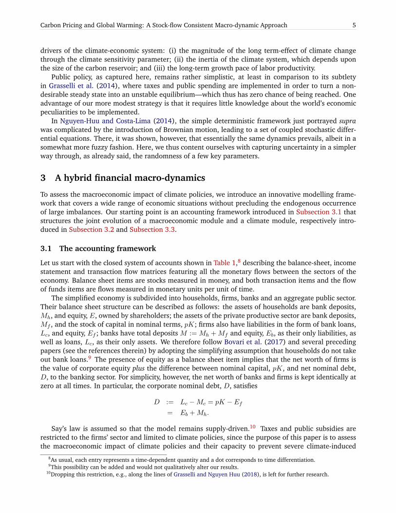
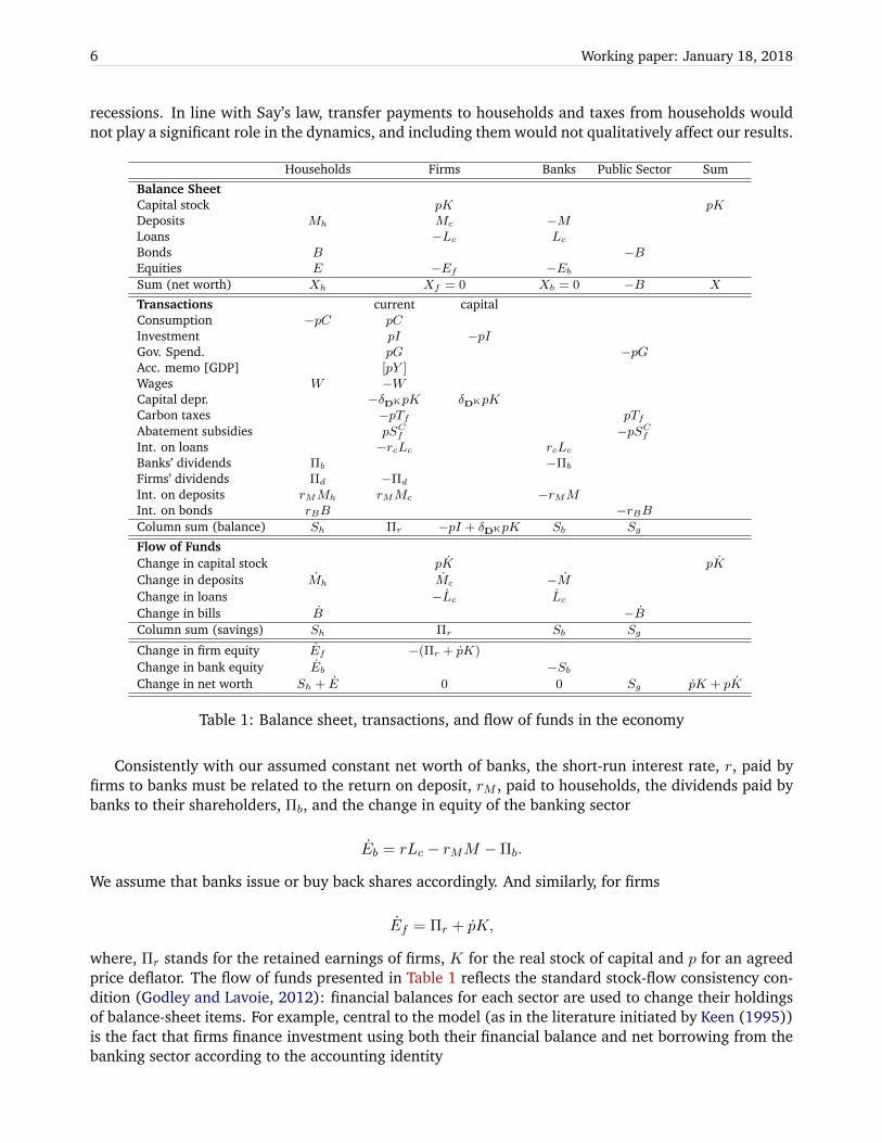
Let us start with the closed system of accounts shown in Table 1,8 describing the balance-sheet, incomestatement and transaction flow matrices featuring all the monetary flows between the sectors of theeconomy. Balance sheet items are stocks measured in money, and both transaction items and the flowof funds items are flows measured in monetary units per unit of time.
The simplified economy is subdivided into households, firms, banks and an aggregate public sector.Their balance sheet structure can be described as follows: the assets of households are bank deposits,Mh, and equity, E, owned by shareholders; the assets of the private productive sector are bank deposits,Mf , and the stock of capital in nominal terms, pK; firms also have liabilities in the form of bank loans,Lc, and equity, Ef ; banks have total deposits M := Mh +Mf and equity, Eb, as their only liabilities, aswell as loans, Lc, as their only assets. We therefore follow Bovari et al. (2017) and several precedingpapers (see the references therein) by adopting the simplifying assumption that households do not takeout bank loans.9 The presence of equity as a balance sheet item implies that the net worth of firms isthe value of corporate equity plus the difference between nominal capital, pK, and net nominal debt,D, to the banking sector. For simplicity, however, the net worth of banks and firms is kept identically atzero at all times. In particular, the corporate nominal debt, D, satisfies
D := Lc −Mc = pK − Ef= Eb +Mh.
Say’s law is assumed so that the model remains supply-driven.10 Taxes and public subsidies arerestricted to the firms’ sector and limited to climate policies, since the purpose of this paper is to assessthe macroeconomic impact of climate policies and their capacity to prevent severe climate-induced
8As usual, each entry represents a time-dependent quantity and a dot corresponds to time differentiation.9This possibility can be added and would not qualitatively alter our results.
10Dropping this restriction, e.g., along the lines of Grasselli and Nguyen Huu (2018), is left for further research.
6 Working paper: January 18, 2018
recessions. In line with Say’s law, transfer payments to households and taxes from households wouldnot play a significant role in the dynamics, and including them would not qualitatively affect our results.
Households Firms Banks Public Sector Sum
Balance SheetCapital stock pK pKDeposits Mh Mc −MLoans −Lc LcBonds B −BEquities E −Ef −EbSum (net worth) Xh Xf = 0 Xb = 0 −B X
Transactions current capitalConsumption −pC pCInvestment pI −pIGov. Spend. pG −pGAcc. memo [GDP] [pY ]Wages W −WCapital depr. −δDKpK δDKpKCarbon taxes −pTf pTfAbatement subsidies pSCf −pSCfInt. on loans −rcLc rcLcBanks’ dividends Πb −Πb
Firms’ dividends Πd −Πd
Int. on deposits rMMh rMMc −rMMInt. on bonds rBB −rBBColumn sum (balance) Sh Πr −pI + δDKpK Sb Sg
Flow of FundsChange in capital stock pK pK
Change in deposits Mh Mc −MChange in loans −Lc LcChange in bills B −BColumn sum (savings) Sh Πr Sb Sg
Change in firm equity Ef −(Πr + pK)
Change in bank equity Eb −SbChange in net worth Sh + E 0 0 Sg pK + pK
Table 1: Balance sheet, transactions, and flow of funds in the economy
Consistently with our assumed constant net worth of banks, the short-run interest rate, r, paid byfirms to banks must be related to the return on deposit, rM , paid to households, the dividends paid bybanks to their shareholders, Πb, and the change in equity of the banking sector
Eb = rLc − rMM −Πb.
We assume that banks issue or buy back shares accordingly. And similarly, for firms
Ef = Πr + pK,
where, Πr stands for the retained earnings of firms, K for the real stock of capital and p for an agreedprice deflator. The flow of funds presented in Table 1 reflects the standard stock-flow consistency con-dition (Godley and Lavoie, 2012): financial balances for each sector are used to change their holdingsof balance-sheet items. For example, central to the model (as in the literature initiated by Keen (1995))is the fact that firms finance investment using both their financial balance and net borrowing from thebanking sector according to the accounting identity
Carbon Pricing and Global Warming: A Stock-flow Consistent Macro-dynamic Approach 7
pK −Πr = Lc − Mc = D.
3.2 The financial macro-dynamics
We now turn to the evolution of this macro-monetary accounting backbone by adding a continuous-timedynamics to its key entries.
3.2.1 Production and labour market
Absent climate change, we assume that firms can produce a potential real amount, Y 0, of a uniqueconsumption good by combining the available workforce, N , and capital, K, with complementaryfactors of production
Y 0 := min
{K
ν; aN
}, (1)
where 1/ν > 0 and a stand respectively for (constant) capital productivity and Harrod-neutral labor-augmenting progress.11 Depending on the level of available capital, firms minimise their costs byhiring the required amount of labour at full capacity, L := Y 0
a = Kν , and the employment rate, λ, is
endogenously given, λ := L/N . As defined shortly, industrial activities release CO2-e emissions thatare subject to a carbon tax levied by the public sector. In order to ease the tax burden, the productivesector may engage abatement activities so as to lower their emissions rate. Thus, a proportion, A, ofoutput, Y 0, is removed from the commodity market and used as an intermediate consumption to reduceCO2-e emissions. Moreover, as in Nordhaus (2016), a proportion, DY, of the remaining production isdestroyed by global warming. As a result, the final production level is therefore
Y := (1−DY)(1−A)Y 0. (2)
The global workforce, N , is assumed to grow according to a sigmoid inferred from the 15–64 agegroup in the United Nations scenario
N := δNN
(1− N
N
), (3)
where N is the upper limit of the global workforce and δN drives the convergence speed. Labourproductivity is assumed to grow according to technical progress at an exogenous constant rate
a
a:= α. (4)
Finally, following Grasselli and Nguyen Huu (2018), the link between the real and nominal spheres ofthe economy is provided by two relationships. First, by a short-run Phillips curve12 similar to the oneintroduced in Grasselli and Nguyen Huu (2018)
w
w:= ϕ(λ), (5)
where w is money wage per capita and ϕ(·) will be an increasing real-valued function with a valuein [0; 1] calibrated. Second, denoting the consumption price as p ≥ 0, an inflation dynamics will be
11The constancy of the capital-output ratio is in agreement with most of the post-Keynesian literature devoted to ecologicalmacro-economics (see Hardt and O’Neill (2017)). Allowing for some substitutability between capital and labour, as well asputty-clay technology, is left for future research.
12See, e.g., Mankiw (2010) and Gordon (2014).
8 Working paper: January 18, 2018
introduced, the latter relaxing with a speed, η, towards its long-run value, which is set as a constantmarkup, µ > 1, times the unit labour cost, ω := wL/pY , according to
i :=p
p:= η (µω − 1) . (6)
3.2.2 Emissions, taxation and abatement decisions
The nominal profit before dividends, Π, is defined as nominal output minus the cost of production:Π := pY − wL − δDKpK − rD + pΣ. Total cost is determined by: (i) the money wage bill, wL; (ii)the capital depreciation, δDKpK, with δDK := δ + DK, where δ > 0 stands for the usual depreciationrate and DK for the fraction of capital destroyed by climate change (to be defined shortly); (iii) thedebt service repayment, rD, with r ≥ 0 as the short-run nominal interest rate and D the total nominaldebt of firms; and (iv) the net public money transfers, Σ, to the productive sector, to be defined shortly.For simplicity, a fraction ∆(ω, r, d) ∈ (0, 1) of profit is paid to the households as dividends providedprofits are non-negative. Consequently, the retained earnings of the corporate sector, Πr, are given byΠr := Π − Πd, with Πd := ∆(ω, r, d)pK. Depending on the level, pC , of the carbon price (labelled inUS$2010 per t-CO2-e), firms endogenously choose their emission reduction rate, n ∈ (0, 1). Industrialemissions, expressed in GtCO2-e, are proportional to the potential production, Y 0, according to
Eind := σ(1− n)Y 0, (7)
where σ > 0 refers to the carbon intensity of the economy, which is assumed to follow some exogenoussigmoid function of time. The emission reduction rate, n, then obviously appears as the fraction ofproduction processes that is “de-polluted”.
As in Nordhaus (2016), the abatement technology, A, is assumed to be a convex function of theemission reduction rate normalised by the emission intensity of the economy, σ, and the exogenousprice of a backstop technology, pBS , labelled in US$2010 per t-CO2-e,13 following
A :=σpBSθ
nθ, (8)
where θ > 0 controls the convexity of the cost.Turning to the public sector, two instruments may foster the transition towards a zero-carbon econ-
omy. A carbon tax, TCf := pCEind, may be levied on industrial emissions, Eind, and a fraction, sA,of abatement costs paid by firms, AY 0, may be subsidised by the public sector for a global transferSCf := sAAY
0. As a result, net transfers from the public to the private sector read
Σ := SCf − TCf . (9)
Faced with the various policy instruments implemented by the public sector, firms choose the emissionreduction rate, n, that minimises abatement costs plus carbon tax,
minn∈[0,1]
AY 0 + TCf − SCf s.t.
A = σpBS
θ nθ
TCf = pCσ(1− n)Y 0
SCf = sAAY0.
Consequently, the optimal aggregate abatement rate of emissions writes
n = min
{(pC
(1− sA)pBS
) 1θ−1
.1
}. (10)
13For the sake of precision, pBS grows at a constant (negative) rate, δpBS .
Carbon Pricing and Global Warming: A Stock-flow Consistent Macro-dynamic Approach 9
Notice that, as expected, the public sector’s subsidies for abatement costs actually accelerate the optimalrate, n, of abatement efforts. From the perspective of firms, the price of the backstop technology isindeed lowered by the subsidies.
3.2.3 Investment and capital accumulation
Turning to investment, let us define the return on assets, πK , by
πK := Π/pK,
=1
ν
((1−DY)(1−A) (1− ω − rd)− pCσ(1− n) + sAA
)− δDK ,
where ω := wL/(pY ) is the wage-to-output ratio and d := D/(pY ) the debt-to-output ratio. Notice thatthe return on assets responds negatively to most of the variables related to climate change, namely A,DY and pc. On the other hand, the reduction of emissions will boost the profit rate.
Following Dafermos et al. (2017)’s insights, aggregate real demand for gross investment, ID, is thendriven by the return on assets, πK , capturing the risk appetite of the productive sector
Id := κ(ω, d, r)Y, (11)
where κ(.) is an increasing function (depending here on our state variables, ω, d and r) with a value in[0; 1] calibrated. Current profits may not suffice to finance the whole of Id, in which case firms will haveto borrow from the banking sector. Due to possibility of credit rationing, however, Id might be onlypartially financed, as defined shortly. Let I refer to the real supply of investment I := Πr/p + D/p +δDKK, where D is the flow of credit granted by the banking sector. Capital accumulation then takesthe standard form
K := I − δDKK. (12)
3.2.4 The banking sector
In order to finance gross investment and their various financial expenses, firms address an aggregatecredit demand, Dd, to the banking sector
Dd := pId + srepD − δDKpK −Πr,
where srepD refers to the fraction of principal, D, that the productive sector has to pay back at eachtime instant to the loan holders (which, for simplicity are identified as being the banking sector).14
As in Dafermos et al. (2017), the banks will satisfy this demand up to a credit rationing function,CR := τ(lev), where τ(·) is an increasing function (with a value in [0, 1]) of the leverage ratio, lev:= D
pK . It provides an upper-bound endogenously set by banks on the supply of additional credit toborrowers, according to their debt-to-capital ratio.15 The aggregate nominal debt dynamics is thereforegiven by
D := (1− CR)Dd − srepD. (13)
As a consequence, effective gross credit can be written as a fraction of available world income, Y :
I = CR(Πr/p+ δDKK − srepD/p
)+ (1− CR)Id
=: κI(CR,ω, πK ,DK,DY, A, d, λ, r, δ, srep)Y. (14)
It can be readily seen from Eq. (14) that the function κI(·) generalises the investment behaviour firstintroduced, with no credit rationing, by Keen (1995).
14Making the yield curve and the schedule of capital repayments explicit would lead to a partial differential equation in aninfinite-dimensional framework, which is left for further research.
15An alternative modelling option would consist in endogenising default and collateral constraints, following, e.g.,Geanakoplos and Zame (2014).
10 Working paper: January 18, 2018
3.2.5 Public sector and policies
The influence of the public sector is summarised by three variables: the real carbon price, pC , thecarbon-abatement subsidy rate, sa, and the short term nominal interest rate, r. Each of these variablesaffects the profit share, hence the entire macro-dynamics through investment flows. For our baselineframework, we assume that the real price of carbon, pC , grows exogenously at a given rate. For thepurpose of our policy scenarios, this price will then be assumed to follow an exogenous path givenby the High-Level Commission on Carbon Prices (2017). For simplicity, the subsidising part of stateintervention (i.e., sa) will also be assumed to be constant throughout. Finally, the short-term interestrate will follow a standard Taylor rule (Taylor, 1993)
r = max {0, r∗ + i+ φ(i− i∗)} , (15)
where r∗ is the long-term real interest rate, i∗ the inflation rate commonly targeted by the monetarypolicy authority16 and φ > 0 a parameter that controls the magnitude of the central bank’s response toinflation.
3.3 Introducing global warming and feedback
Climate change is modelled in a stylised way directly inspired by the DICE model of Nordhaus (2016),adapted here to our continuous-time setting. Both the macroeconomic and climate modules are thencoupled through the damage function already introduced in Eq. (2).
3.3.1 The climate module
Global emissions, E := Eind + Eland, are expressed in CO2-e units and result from two sources: (i)industrial emissions, Eind, defined in Eq. (7); and (ii) exogenous land-use emissions, Eland, decreasingat an exponential rate, δEland < 0, such that Eland := δElandEland. The emission intensity of theeconomy, σ, also follows an exogenous path given by σ := gσσ and gσ := gσδgσ , with δgσ < 0 aparameter.
The carbon cycle is described through a three-layer model that features the interactions between:(i) the atmosphere (layer AT ), where emissions are released, (ii) the biosphere–upper ocean (layerUP ) and (iii) the lower ocean (layer LO) the latter two acting as carbon sinks. Thus, in each layeri ∈ {AT,UP,LO}, the accumulation of CO2
i evolves according to ˙CO2AT
˙CO2UP
˙CO2LO
:=
E00
+ Φ
COAT2
COUP2
COLO2
with Φ :=
−φ12 φ12CATUP 0
φ12 −φ12CATUP − φ23 φ23C
UPLO
0 φ23 −φ23CUPLO
,(16)
where Cji :=CjpindCipind
, i, j ∈ {AT,UP,LO}, with Cipind denoting the pre-industrial CO2-e concentration
in the corresponding layer, i, and φij standing for the diffusion coefficients between layers i and j.The energy imbalance with regards to pre-industrial levels induces a radiative forcing in the atmo-
spheric layer. The latter is composed of two terms: (i) an industrial forcing, Find :=F2×CO2log(2) ln
(COAT2CATpind
),
where F2×CO2 stands for the forcing resulting from a doubling of the pre-industrial atmospheric con-centration in CO2-e and (ii) an exogenous radiative forcing, Fexo, which grows linearly from its initialvalue to a plateau in 2100 as in Nordhaus (2016).
16Which might be thought of as the network of central banks.
Carbon Pricing and Global Warming: A Stock-flow Consistent Macro-dynamic Approach 11
The dynamics of temperature is given by a two-layer model describing the interplay between theatmosphere and upper ocean (resp. the lower ocean), with a mean temperature deviation, T (resp.T0), with regards to the pre-industrial era
CT := F − ρT − γ∗(T − T0), (17)
C0T0 := γ∗(T − T0), (18)
where ρ is the radiative feedback parameter, and γ∗ is the heat exchange coefficient between the twolayers. C and C0, refer respectively to the heat capacity of the atmosphere, land surface and upperocean layer, and to the heat capacity of the deep ocean layer. Observe that, within such a set-up, theequilibrium climate sensitivity (ECS) is defined by S := F2×CO2/ρ.
3.4 Climate feedback-loop
In order to quantify the impact of global warming on the world economy, we again follow Nordhaus(2016) and adopt a damage function, D(·), summarising the total economic feedback of environmentalchange:
D := 1− 1
1 + π1T + π2T 2 + π3T ζ3. (19)
with π1, π2, π3, ζ3 ≥ 0. As argued by Stern (2013) and Dietz and Stern (2015), global warming mayhave an adverse repercussion not only on income but also on the factors of production themselves,such as capital, and especially on infrastructure. Following Dietz and Stern (2015), we therefore divideglobal damages, D(·), into two components, one impacting the capital stock
DK := fK D, fK ∈ (0; 1), (20)
while its complement affects the gross output, Y :
DY := 1− 1−D
1−DK. (21)
4 Uncertainty and policy scenarios
Uncertainties on climate and economic growth are introduced in this section along with the differentprospective rundowns that will frame our numerical analysis.
4.1 Climate and economic uncertainties
Uncertainty is made explicit for three main drivers of the climate-economic system: (i) the magnitudeof the long-term effect of climate change captured through the climate sensitivity parameter, S;17 (ii)the inertia of the climate system, which depends upon the size of the intermediate carbon reservoir,CUPpind; and (iii) the long-term growth rate of labour productivity, α.18 The above parameters havebeen extensively discussed in the climate and integrated assessment literature.19 Various estimates of
17S characterises the Earth’s long-term, thermo-dynamic equilibrium global temperature response to a doubling of the pre-industrial CO2 atmospheric concentration. Therefore, in the medium run, only probability estimates can be deduced fromempirical observation.
18The allocation of climate impairments between output and capital will also be introduced in a subsequent section throughthe parameter fK (see 20).
19See Knutti et al. (2017) and the references therein.
12 Working paper: January 18, 2018
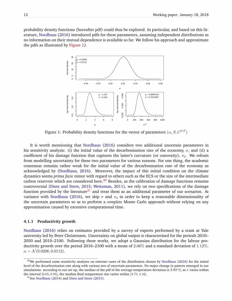
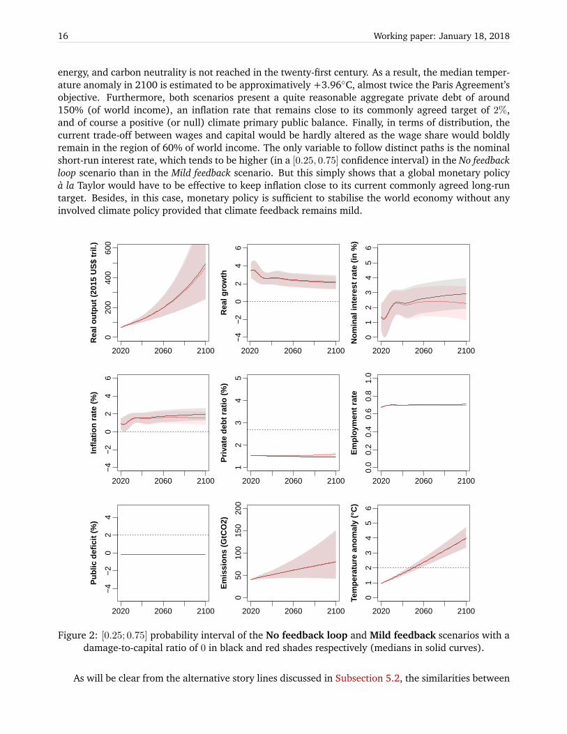
probability density functions (hereafter pdf) could thus be explored. In particular, and based on this lit-erature, Nordhaus (2016) introduced pdfs for these parameters, assuming independent distributions asno information on their mutual dependence is available so far. We follow his approach and approximatethe pdfs as illustrated by Figure 1).
−0.04 −0.02 0.00 0.02 0.04 0.06 0.08
05
1525
35
α
Nor
mal
den
sity
µ = 0.0206σ = 0.0112
0 2 4 6 8
0.0
0.2
0.4
S
log−
Nor
mal
den
sity
µ = 1.107σ = 0.264
0 200 400 600 800 10000.
000
0.00
20.
004
Cup
log−
Nor
mal
den
sity
µ = 5.8855763σ = 0.2512867
Figure 1: Probability density functions for the vector of parameters (α, S,CUP )
It is worth mentioning that Nordhaus (2016) considers two additional uncertain parameters inhis sensitivity analysis: (i) the initial value of the decarbonisation rate of the economy, σ, and (ii) acoefficient of his damage function that captures the latter’s curvature (or convexity), π2. We refrainfrom modelling uncertainty for these two parameters for various reasons. For one thing, the academicconsensus remains rather weak for the initial value of the decarbonisation rate of the economy asacknowledged by (Nordhaus, 2016). Moreover, the impact of this initial condition on the climatedynamics seems prima facie minor with regard to others such as the ECS or the size of the intermediatecarbon reservoir which are considered here.20 Besides, as the calibration of damage functions remainscontroversial (Dietz and Stern, 2015; Weitzman, 2011), we rely on two specifications of the damagefunction provided by the literature21 and treat them as an additional parameter of our scenarios. Atvariance with Nordhaus (2016), we skip σ and π2 in order to keep a reasonable dimensionality ofthe uncertain parameters so as to perform a complete Monte Carlo approach without relying on anyapproximation caused by excessive computational time.
4.1.1 Productivity growth
Nordhaus (2016) relies on estimates provided by a survey of experts performed by a team at Yaleuniversity led by Peter Christensen. Uncertainty on global output is characterised for the periods 2010–2050 and 2010–2100. Following these works, we adopt a Gaussian distribution for the labour pro-ductivity growth over the period 2016–2100 with a mean of 2.06% and a standard deviation of 1.12%:α ∼ N (0.0206, 0.0112).
20We performed some sensitivity analyses on extreme cases of the distribution chosen by Nordhaus (2016) for the initiallevel of the decarbonisation rate along with various sets of uncertain parameters. No major change in pattern emerged in oursimulations: according to our set-up, the median of the pdf of the average temperature deviation is 3.93◦C; as σ varies withinthe interval [0.05, 0.95], the median final temperature rise varies within [3.75, 4.16].
21See Nordhaus (2014) and Dietz and Stern (2015).
Carbon Pricing and Global Warming: A Stock-flow Consistent Macro-dynamic Approach 13
4.1.2 Equilibrium climate sensitivity (ECS)
The intrinsic uncertainty of the transient response of the climate system is captured by the ECS param-eter.22 We assume that the ECS follows a log-Gaussian distribution with µ = 1.107 and σ = 0.264. Inother words, S ∼ log−N (1.107, 0.264)—a choice motivated by the Bayesian estimates from Gillinghamet al. (2015).
4.1.3 Carbon cycle
If many parameters of the carbon cycle are uncertain, the most important one remains the size of theintermediate reservoir (biosphere and upper level of the oceans), CUPpind in our setup. This parameterwill quantify the maximal upper level of the ocean capacity of CO2 or, in other words, the inertia of theclimate system. To take into account the uncertainty for this parameter, we follow the work of Nordhaus(2016), aimed at mimicking the results from Friedlingstein et al. (2014) in the difference of concentra-tion in 2100 using the RCP8.5 CO2 emissions. We thus calibrate a log-Gaussian distribution that is theclosest to the quantiles reported by Nordhaus. In other words, CUPpind ∼ log−N (5.8855763, 0.2512867).
4.2 Climate risk
We finally consider the risks pervading the magnitude of climate damage to the economy and its channelof transmission. Indeed, as already said, climate change may impair output either directly or indirectlythrough various forms of harm to capital stock, which could in turn trigger potential contagion effectson the financial dynamics of the economy. We explore this channel by first testing two specificationsof the aggregate damage function. The first is provided by Nordhaus (2016) and considered as abenchmark (labelled Mild) for our analysis as its validity is limited to a moderate range of globalwarming. However, as argued by Stern (2013), climate thresholds might be reached for higher rangesof temperature deviation, typically greater than +4◦C—potentially giving rise to more severe and non-linear consequences. We thus also consider the more convex specification of the damage functionintroduced by Dietz and Stern (2015). Regarding the allocation of damages between output and capital,we consider the educated guess provided by Dietz and Stern (2015)’s interpretation of the resultsobtained byNordhaus and Boyer (2000), which are in the region of 1/3. This means that capital stocksustains a third of the damages (in consumption-equivalent terms). We consequently test two differentvalues: fK ∈ {0, 1/3} and take fK = 0 as a reference point in order to facilitate comparison with earlierworks such as Nordhaus (2016).
4.3 Public policy scenarios
First, we consider a No feedback scenario yielding a flow of trajectories absent any climate-change feed-back loop. This scenario is then put in perspective with a Mild feedback scenario, introducing Nordhaus’specification for the damage function, along with a low real carbon tax growing at a constant 2% peryear, in line with the Baseline scenario of Nordhaus (2014)). This second scenario is viewed as anintermediary step toward a baseline scenario incorporating climate feedback, and allows us to discussthe choice of a damage function. We finally introduce the three public policy scenarios considered inthis paper: a scenario with a carbon tax calibrated from the High-Level Commission on Carbon Prices(2017) (labelled Moderate public policy), and a combination of the same carbon tax plus a subsidyfor the backstop technology (called Involved public policy). The two corresponding narratives are con-
22For the calibration of the model, the heat capacity of the atmosphere, C, is updated according to climate sensitivity inorder to adjust the TCR with the ECS as in Nordhaus and Sztorc (2013). Furthermore, carbon storage is precluded from theanalysis.
14 Working paper: January 18, 2018
trasted with a Soft public policy baseline where public intervention is again limited to a low real carbontax growing at a constant 2% per year, in line with the Baseline scenario of Nordhaus (2014)).
As mentioned in the Introduction of this paper, theHigh-Level Commission on Carbon Prices (2017)has recommended a corridor of carbon price levels meant to be consistent with achieving the Paristemperature target and the Sustainable Development Goals: from at least US$40-80/tCO2 by 2020 toUS$50-100/tCO2 by 2030.23 In our simulations, we will focus on the upper barrier of the price corridor(hereafter High pC). We stress that, as we take a long-term perspective, our simulations run from 2016to 2100, while the recommendations of the High-Level Commission on Carbon Prices (2017) remainconfined within the 2030 horizon in line with the Paris Agreement. Linear interpolations of the carbonprice are therefore assumed to be outside the recommendation time range. Furthermore, as alreadysaid, we also consider public subsidies for mitigation technologies. The public sector subsidises theabatement cost as captured via Eq. (10). This subsidy could be interpreted as being funded by thecarbon tax and thus viewed from firms’ side as a price reduction on the abatement technology frompBS to (1− sa)pBS .
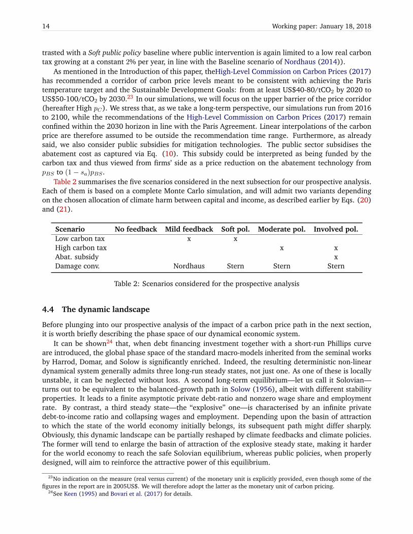
Table 2 summarises the five scenarios considered in the next subsection for our prospective analysis.Each of them is based on a complete Monte Carlo simulation, and will admit two variants dependingon the chosen allocation of climate harm between capital and income, as described earlier by Eqs. (20)and (21).
Scenario No feedback Mild feedback Soft pol. Moderate pol. Involved pol.Low carbon tax x xHigh carbon tax x xAbat. subsidy xDamage conv. Nordhaus Stern Stern Stern
Table 2: Scenarios considered for the prospective analysis
4.4 The dynamic landscape
Before plunging into our prospective analysis of the impact of a carbon price path in the next section,it is worth briefly describing the phase space of our dynamical economic system.
It can be shown24 that, when debt financing investment together with a short-run Phillips curveare introduced, the global phase space of the standard macro-models inherited from the seminal worksby Harrod, Domar, and Solow is significantly enriched. Indeed, the resulting deterministic non-lineardynamical system generally admits three long-run steady states, not just one. As one of these is locallyunstable, it can be neglected without loss. A second long-term equilibrium—let us call it Solovian—turns out to be equivalent to the balanced-growth path in Solow (1956), albeit with different stabilityproperties. It leads to a finite asymptotic private debt-ratio and nonzero wage share and employmentrate. By contrast, a third steady state—the “explosive” one—is characterised by an infinite privatedebt-to-income ratio and collapsing wages and employment. Depending upon the basin of attractionto which the state of the world economy initially belongs, its subsequent path might differ sharply.Obviously, this dynamic landscape can be partially reshaped by climate feedbacks and climate policies.The former will tend to enlarge the basin of attraction of the explosive steady state, making it harderfor the world economy to reach the safe Solovian equilibrium, whereas public policies, when properlydesigned, will aim to reinforce the attractive power of this equilibrium.
23No indication on the measure (real versus current) of the monetary unit is explicitly provided, even though some of thefigures in the report are in 2005US$. We will therefore adopt the latter as the monetary unit of carbon pricing.
24See Keen (1995) and Bovari et al. (2017) for details.
Carbon Pricing and Global Warming: A Stock-flow Consistent Macro-dynamic Approach 15
Notice that, at variance with the Harrod-Domar knife-edge model, dynamic instability is not theonly possible outcome here. But our approach also departs from the Solow-Swan setting as the Solovianequilibrium is not the only one where the state of the economy may stabilise.25
5 Prospective analysis
In this section, we present the main results of our prospective analysis on the macro-dynamic conse-quences of carbon pricing trajectories and public subsidies. First, we discuss the random paths followedby our key variables and, second, we examine their sustainability by computing the probability of over-shooting two critical thresholds related to financial instability and the Earth’s average temperatureanomaly. The latter analysis allows us to quantify the macroeconomic impact of our policy scenarios.
Obviously, many criteria would deserve to be examined as critical lines. For simplicity, and withthe hope of launching further inquiry on this issue, we discuss only two of them in this paper: (i)a 2◦C temperature anomaly and (ii) a 270% total aggregate private debt ratio on output. In ourview, they are informative on both climate and financial instabilities whose trade-off is the focus ofthis paper. The Paris Agreement set a 2◦C threshold for temperature anomaly based on our currentknowledge (gathered, e.g., by the IPCC26) on tipping points leading to severe and possibly uncontrolleddamages to our economy and environment. On the other hand, our modelling approach also explicitlyconsiders the financial channel as a cause of possible recession. At the level of an individual firm,whenever its liabilities exceed its assets, a company will arguably default on its debt (Geanakoplos andZame (2014)). At the aggregate level, one can therefore consider that, if global private debt were toexceed the aggregate stock of capital, the global financial sphere would incur a serious risk of systemicdefaults.27 Using the Penn World Table (Feenstra et al., 2015), we calibrate the current global averagecapital-to-GDP ratio, ν, at 2.7. Since this ratio is constant in our modelling approach, it will play therole of the debt-to-output threshold we are looking for. As only part of our Monte Carlo simulationsstay safely below these two specific ceilings, we shall compute the probability of overshooting them asan indicator of the underlying sustainability of the climate policies.
5.1 Is climate change really harmless in the long run?
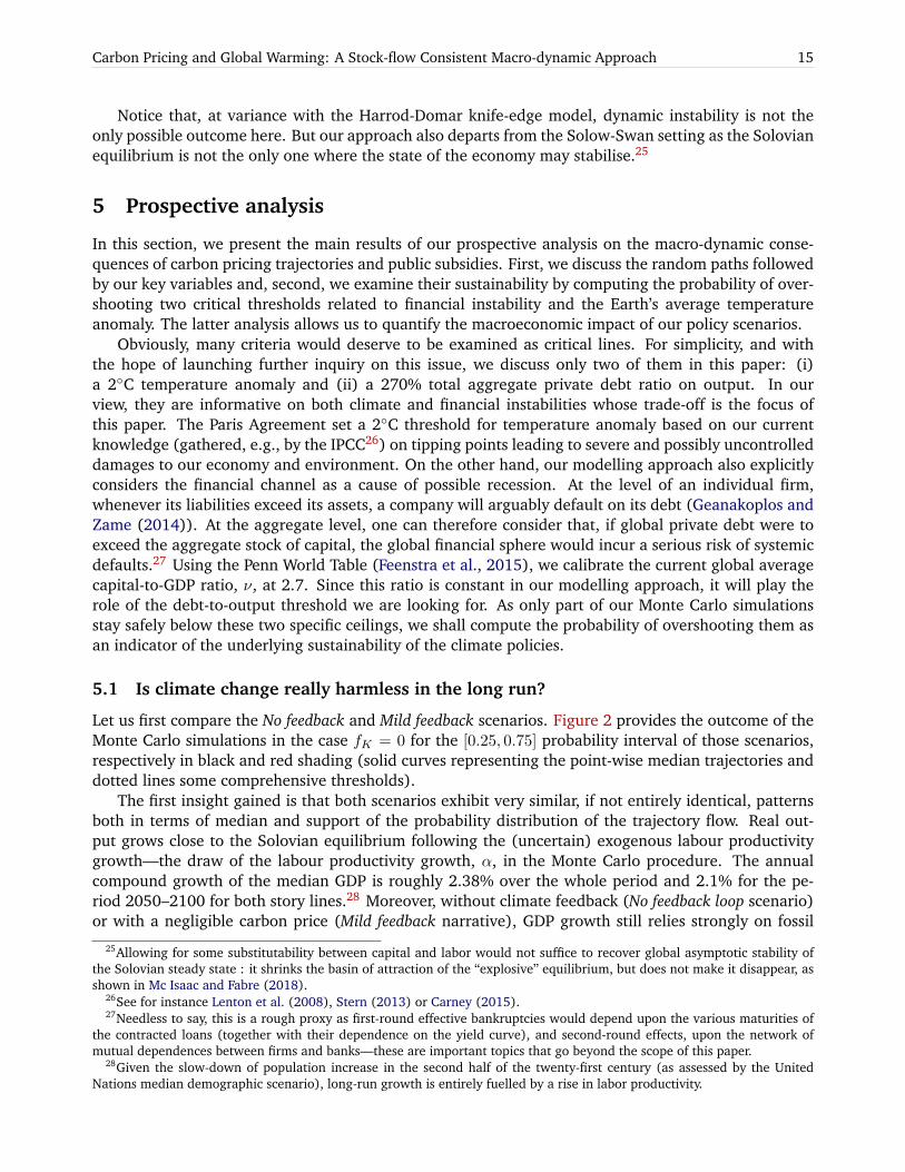
Let us first compare the No feedback and Mild feedback scenarios. Figure 2 provides the outcome of theMonte Carlo simulations in the case fK = 0 for the [0.25, 0.75] probability interval of those scenarios,respectively in black and red shading (solid curves representing the point-wise median trajectories anddotted lines some comprehensive thresholds).
The first insight gained is that both scenarios exhibit very similar, if not entirely identical, patternsboth in terms of median and support of the probability distribution of the trajectory flow. Real out-put grows close to the Solovian equilibrium following the (uncertain) exogenous labour productivitygrowth—the draw of the labour productivity growth, α, in the Monte Carlo procedure. The annualcompound growth of the median GDP is roughly 2.38% over the whole period and 2.1% for the pe-riod 2050–2100 for both story lines.28 Moreover, without climate feedback (No feedback loop scenario)or with a negligible carbon price (Mild feedback narrative), GDP growth still relies strongly on fossil
25Allowing for some substitutability between capital and labor would not suffice to recover global asymptotic stability ofthe Solovian steady state : it shrinks the basin of attraction of the “explosive” equilibrium, but does not make it disappear, asshown in Mc Isaac and Fabre (2018).
26See for instance Lenton et al. (2008), Stern (2013) or Carney (2015).27Needless to say, this is a rough proxy as first-round effective bankruptcies would depend upon the various maturities of
the contracted loans (together with their dependence on the yield curve), and second-round effects, upon the network ofmutual dependences between firms and banks—these are important topics that go beyond the scope of this paper.
28Given the slow-down of population increase in the second half of the twenty-first century (as assessed by the UnitedNations median demographic scenario), long-run growth is entirely fuelled by a rise in labor productivity.
16 Working paper: January 18, 2018
energy, and carbon neutrality is not reached in the twenty-first century. As a result, the median temper-ature anomaly in 2100 is estimated to be approximatively +3.96◦C, almost twice the Paris Agreement’sobjective. Furthermore, both scenarios present a quite reasonable aggregate private debt of around150% (of world income), an inflation rate that remains close to its commonly agreed target of 2%,and of course a positive (or null) climate primary public balance. Finally, in terms of distribution, thecurrent trade-off between wages and capital would be hardly altered as the wage share would boldlyremain in the region of 60% of world income. The only variable to follow distinct paths is the nominalshort-run interest rate, which tends to be higher (in a [0.25, 0.75] confidence interval) in the No feedbackloop scenario than in the Mild feedback scenario. But this simply shows that a global monetary policya la Taylor would have to be effective to keep inflation close to its current commonly agreed long-runtarget. Besides, in this case, monetary policy is sufficient to stabilise the world economy without anyinvolved climate policy provided that climate feedback remains mild.
2020 2060 2100
020
040
060
0
Rea
l out
put (
2015
US
$ tr
il.)
2020 2060 2100
−4
−2
02
46
Rea
l gro
wth
2020 2060 2100
01
23
45
6
Nom
inal
inte
rest
rat
e (in
%)
2020 2060 2100
−4
−2
02
46
Infla
tion
rate
(%
)
2020 2060 2100
12
34
5
Priv
ate
debt
rat
io (
%)
2020 2060 2100
0.0
0.2
0.4
0.6
0.8
1.0
Em
ploy
men
t rat
e
2020 2060 2100
−4
−2
02
4
Pub
lic d
efic
it (%
)
2020 2060 2100
050
100
150
200
Em
issi
ons
(GtC
O2)
2020 2060 2100
01
23
45
6
Tem
pera
ture
ano
mal
y (°
C)
Figure 2: [0.25; 0.75] probability interval of the No feedback loop and Mild feedback scenarios with adamage-to-capital ratio of 0 in black and red shades respectively (medians in solid curves).
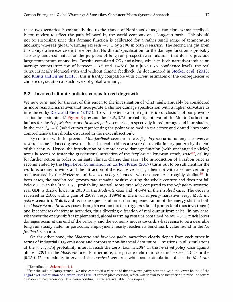
As will be clear from the alternative story lines discussed in Subsection 5.2, the similarities between
Carbon Pricing and Global Warming: A Stock-flow Consistent Macro-dynamic Approach 17
these two scenarios is essentially due to the choice of Nordhaus’ damage function, whose feedbackis too modest to affect the path followed by the world economy on a long-run basis. This shouldnot be surprising since this damage function is calibrated for a rather small range of temperatureanomaly, whereas global warming exceeds +3◦C by 2100 in both scenarios. The second insight fromthis comparative exercise is therefore that Nordhaus’ specification for the damage function is probablyseriously underestimated for the purposes of long-run prospective simulations that do not precludelarge temperature anomalies. Despite cumulated CO2 emissions, which in both narratives induce anaverage temperature rise of between +3.5 and +4.5◦C (at a [0.25, 0.75] confidence level), the realoutput is nearly identical with and without climate feedback. As documented in Stocker et al. (2013)and Knutti and Fisher (2015), this is hardly compatible with current estimates of the consequences ofclimate degradation at such levels of global warming.
5.2 Involved climate policies versus forced degrowth
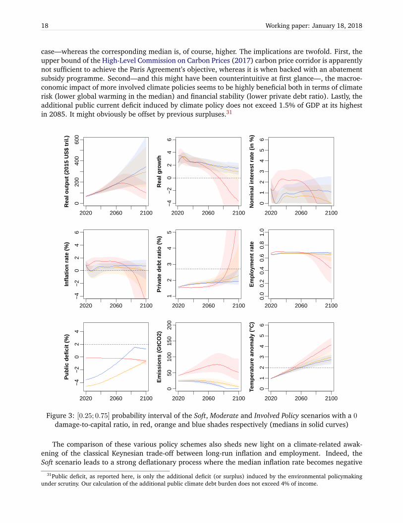
We now turn, and for the rest of this paper, to the investigation of what might arguably be consideredas more realistic narratives that incorporate a climate damage specification with a higher curvature asintroduced by Dietz and Stern (2015). To what extent can the optimistic conclusions of our previoussection be maintained? Figure 3 presents the [0.25, 0.75] probability interval of the Monte Carlo simu-lations for the Soft, Moderate and Involved policy scenarios, respectively in red, orange and blue shades,in the case fK = 0 (solid curves representing the point-wise median trajectory and dotted lines somecomprehensive thresholds, discussed in the next subsection).
By contrast with the previous Mild feedback scenario, the Soft policy scenario no longer convergestowards some balanced growth path: it instead exhibits a severe debt-deflationary pattern by the endof this century. Hence, the introduction of a more severe damage function (with unchanged policies)actually seems to foster the gravitational attraction of the “explosive” long-run steady state29, callingfor further action in order to mitigate climate change damages. The introduction of a carbon price asrecommended by the High-Level Commission on Carbon Prices (2017) turns out to be sufficient for theworld economy to withstand the attraction of the explosive basin, albeit not with absolute certainty,as illustrated by the Moderate and Involved policy schemes—whose outcome is roughly similar.30 Inboth cases, the median real growth rate remains positive during the whole century and does not fallbelow 0.5% in the [0.25, 0.75] probability interval. More precisely, compared to the Soft policy scenario,real GDP is 3.26% lower in 2050 in the Moderate case and 4.04% in the Involved case. The order isreversed in 2100, with a gain of 250% (resp. 199%) in the Involved policy narrative (resp. Moderatepolicy scenario). This is a direct consequence of an earlier implementation of the energy shift in boththe Moderate and Involved cases through a carbon tax that triggers a fall of profits (and thus investment)and incentivises abatement activities, thus diverting a fraction of real output from sales. In any case,whenever the energy shift is implemented, global warming remains contained below +3◦C, much lowerdamages occur at the end of the century, and the economy moves towards what seems to be a desirablelong-run steady state. In particular, employment nearly reaches its benchmark value found in the Nofeedback scenario.
On the other hand, the Moderate and Involved policy narratives clearly depart from each other interms of industrial CO2 emissions and corporate non-financial debt ratios. Emissions in all simulationsof the [0.25, 0.75] probability interval reach the zero floor in 2084 in the Involved policy case againstalmost 2091 in the Moderate one. Furthermore, the private debt ratio does not exceed 270% in the[0.25, 0.75] probability interval of the Involved scenario, while some simulations do in the Moderate
29Described in Subsection 4.4.30For the sake of completeness, we also computed a variant of the Moderate policy scenario with the lower bound of the
High-Level Commission on Carbon Prices (2017) carbon price corridor, which was shown to be insufficient to preclude severeclimate-induced recessions. The corresponding figures are available upon request.
18 Working paper: January 18, 2018
case—whereas the corresponding median is, of course, higher. The implications are twofold. First, theupper bound of the High-Level Commission on Carbon Prices (2017) carbon price corridor is apparentlynot sufficient to achieve the Paris Agreement’s objective, whereas it is when backed with an abatementsubsidy programme. Second—and this might have been counterintuitive at first glance—, the macroe-conomic impact of more involved climate policies seems to be highly beneficial both in terms of climaterisk (lower global warming in the median) and financial stability (lower private debt ratio). Lastly, theadditional public current deficit induced by climate policy does not exceed 1.5% of GDP at its highestin 2085. It might obviously be offset by previous surpluses.31
2020 2060 2100
020
040
060
0
Rea
l out
put (
2015
US
$ tr
il.)
2020 2060 2100
−4
−2
02
46
Rea
l gro
wth
2020 2060 2100
01
23
45
6
Nom
inal
inte
rest
rat
e (in
%)
2020 2060 2100
−4
−2
02
46
Infla
tion
rate
(%
)
2020 2060 2100
12
34
5
Priv
ate
debt
rat
io (
%)
2020 2060 2100
0.0
0.2
0.4
0.6
0.8
1.0
Em
ploy
men
t rat
e
2020 2060 2100
−4
−2
02
4
Pub
lic d
efic
it (%
)
2020 2060 2100
050
100
150
200
Em
issi
ons
(GtC
O2)
2020 2060 2100
01
23
45
6
Tem
pera
ture
ano
mal
y (°
C)
Figure 3: [0.25; 0.75] probability interval of the Soft, Moderate and Involved Policy scenarios with a 0damage-to-capital ratio, in red, orange and blue shades respectively (medians in solid curves)
The comparison of these various policy schemes also sheds new light on a climate-related awak-ening of the classical Keynesian trade-off between long-run inflation and employment. Indeed, theSoft scenario leads to a strong deflationary process where the median inflation rate becomes negative
31Public deficit, as reported here, is only the additional deficit (or surplus) induced by the environmental policymakingunder scrutiny. Our calculation of the additional public climate debt burden does not exceed 4% of income.
Carbon Pricing and Global Warming: A Stock-flow Consistent Macro-dynamic Approach 19
shortly after 2080—and its worst case distribution tail even plunges below -4% during the last decadeof the century—whereas underemployment reaches a hardly politically sustainable 60%. By contrast,the other two scenarios exhibit non-negative inflation rates throughout and employment rates that re-main in the neighbourhood of today’s 65%. In the best tail of the probability distribution of the Involvedpolicy story line, inflation even remains close to the iconic 2%. Consequently, no analog of a vertical“long-run Phillips curve” can be observed in our setting. Hence, the structural long-run underemploy-ment rate (around 35%), which still seems to hold in the vicinity of the Solovian steady state (towardswhich the Involved paths wander), should not be confused with the celebrated “natural rate of unem-ployment” introduced in Friedman (1968) and Phelps (1968). Moreover, the carbon price togetherwith a monetary policy captured here through the setting of r do play a role, even in the long run, sincethey influence the asymptotic local stability of the balanced growth path. This contrasts with the veryconcept of “natural unemployment”, which embodies the idea that any public policy whatsoever wouldbe ineffective in reducing underemployment. Actually, our structural unemployment rate is closer tothe NAIRU (“Non-Acccelerating Inflation Rate of Unemployment”) introduced in Tobin (1980), since,at the balanced growth path, inflation stabilises.
5.3 Staying under reasonable climate-economic thresholds
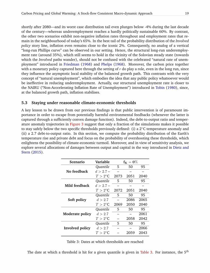
A key lesson to be drawn from our previous findings is that public intervention is of paramount im-portance in order to escape from potentially harmful environmental feedbacks (whenever the latter iscaptured through a sufficiently convex damage function). Indeed, the debt-to-output ratio and temper-ature anomaly trajectories in Figure 3 suggest that only a fraction of the simulations makes it possibleto stay safely below the two specific thresholds previously defined: (i) a 2◦C temperature anomaly and(ii) a 2.7 debt-to-output ratio. In this section, we compute the probability distribution of the Earth’stemperature rise and private debt and focus on the probability of overshooting these thresholds, whichenlightens the possibility of climate-economic turmoil. Moreover, and in view of sensitivity analysis, weexplore several allocations of damages between output and capital in the way introduced in Dietz andStern (2015).
Scenario Variable fK = 0%
Quantile 5 50 95No feedback d > 2.7 – – – –
T > 2◦C 2073 2051 2040Quantile 5 50 95
Mild feedback d > 2.7 – – – –T > 2◦C 2072 2051 2040Quantile 5 50 95
Soft policy d > 2.7 – 2086 2065T > 2◦C 2069 2050 2040Quantile 5 50 95
Moderate policy d > 2.7 – – 2061T > 2◦C – 2058 2042Quantile 5 50 95
Involved policy d > 2.7 – – 2066T > 2◦C – 2059 2043
Table 3: Dates at which thresholds are reached
The date at which a threshold is hit for a given quantile is given in Table 3. For instance, the 5th
20 Working paper: January 18, 2018
quantile of the random distribution of temperature rise induced by the No feedback loop scenario crossesthe +2◦C limit in 2073. As expected, for the 95th quantile, the same cutoff point is reached no laterthan 2040. Three comments on Table 3 are in order: First, as expected, the deeper the public sector’sinvolvement in fighting against climate change, the later the +2◦C target is reached. For instance, onlyModerate and Involved policy narratives make it possible to have more than a 5% chance of staying belowthe +2◦C target until the end of this century. Second, the No feedback and Mild feedback scenarios showvery similar dates, echoing our previous remarks. Third, for a sufficiently convex damage function,public policy involvement helps to delay the time at which the debt-to-output 2.7 deadline would bereached in the higher part of the probability distribution.
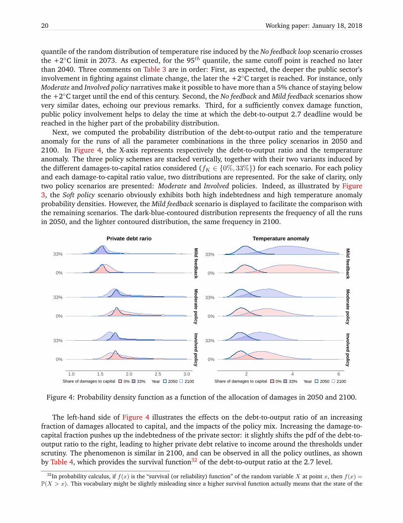
Next, we computed the probability distribution of the debt-to-output ratio and the temperatureanomaly for the runs of all the parameter combinations in the three policy scenarios in 2050 and2100. In Figure 4, the X-axis represents respectively the debt-to-output ratio and the temperatureanomaly. The three policy schemes are stacked vertically, together with their two variants induced bythe different damages-to-capital ratios considered (fK ∈ {0%, 33%}) for each scenario. For each policyand each damage-to-capital ratio value, two distributions are represented. For the sake of clarity, onlytwo policy scenarios are presented: Moderate and Involved policies. Indeed, as illustrated by Figure3, the Soft policy scenario obviously exhibits both high indebtedness and high temperature anomalyprobability densities. However, the Mild feedback scenario is displayed to facilitate the comparison withthe remaining scenarios. The dark-blue-contoured distribution represents the frequency of all the runsin 2050, and the lighter contoured distribution, the same frequency in 2100.
Mild feedback
Moderate policy
Involved policy
1.0 1.5 2.0 2.5 3.0
0%
33%
0%
33%
0%
33%
Share of damages to capital 0% 33% Year 2050 2100
Private debt rario
Mild feedback
Moderate policy
Involved policy
2 4 6
0%
33%
0%
33%
0%
33%
Share of damages to capital 0% 33% Year 2050 2100
Temperature anomaly
Figure 4: Probability density function as a function of the allocation of damages in 2050 and 2100.
The left-hand side of Figure 4 illustrates the effects on the debt-to-output ratio of an increasingfraction of damages allocated to capital, and the impacts of the policy mix. Increasing the damage-to-capital fraction pushes up the indebtedness of the private sector: it slightly shifts the pdf of the debt-to-output ratio to the right, leading to higher private debt relative to income around the thresholds underscrutiny. The phenomenon is similar in 2100, and can be observed in all the policy outlines, as shownby Table 4, which provides the survival function32 of the debt-to-output ratio at the 2.7 level.
32In probability calculus, if f(x) is the “survival (or reliability) function” of the random variable X at point x, then f(x) =P(X > x). This vocabulary might be slightly misleading since a higher survival function actually means that the state of the
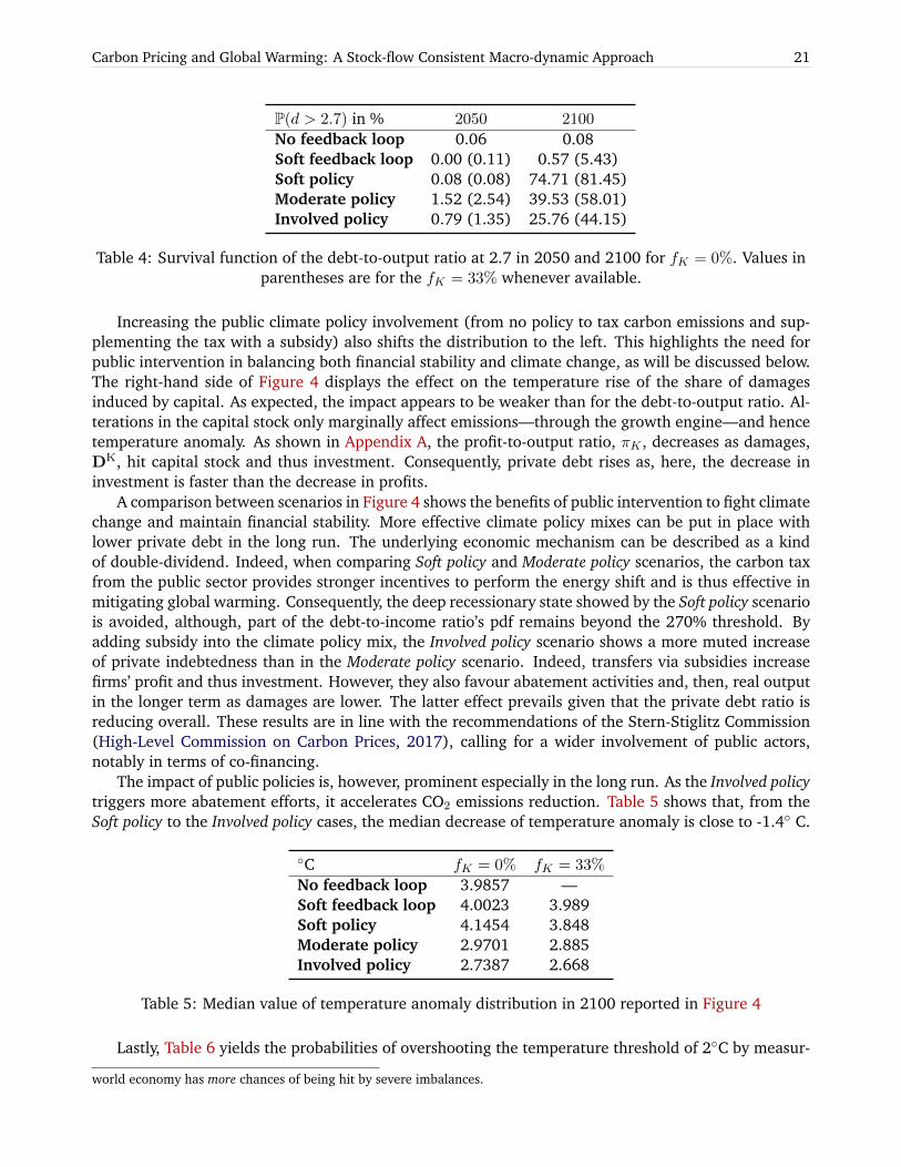
Carbon Pricing and Global Warming: A Stock-flow Consistent Macro-dynamic Approach 21
P(d > 2.7) in % 2050 2100
No feedback loop 0.06 0.08Soft feedback loop 0.00 (0.11) 0.57 (5.43)Soft policy 0.08 (0.08) 74.71 (81.45)Moderate policy 1.52 (2.54) 39.53 (58.01)Involved policy 0.79 (1.35) 25.76 (44.15)
Table 4: Survival function of the debt-to-output ratio at 2.7 in 2050 and 2100 for fK = 0%. Values inparentheses are for the fK = 33% whenever available.
Increasing the public climate policy involvement (from no policy to tax carbon emissions and sup-plementing the tax with a subsidy) also shifts the distribution to the left. This highlights the need forpublic intervention in balancing both financial stability and climate change, as will be discussed below.The right-hand side of Figure 4 displays the effect on the temperature rise of the share of damagesinduced by capital. As expected, the impact appears to be weaker than for the debt-to-output ratio. Al-terations in the capital stock only marginally affect emissions—through the growth engine—and hencetemperature anomaly. As shown in Appendix A, the profit-to-output ratio, πK , decreases as damages,DK, hit capital stock and thus investment. Consequently, private debt rises as, here, the decrease ininvestment is faster than the decrease in profits.
A comparison between scenarios in Figure 4 shows the benefits of public intervention to fight climatechange and maintain financial stability. More effective climate policy mixes can be put in place withlower private debt in the long run. The underlying economic mechanism can be described as a kindof double-dividend. Indeed, when comparing Soft policy and Moderate policy scenarios, the carbon taxfrom the public sector provides stronger incentives to perform the energy shift and is thus effective inmitigating global warming. Consequently, the deep recessionary state showed by the Soft policy scenariois avoided, although, part of the debt-to-income ratio’s pdf remains beyond the 270% threshold. Byadding subsidy into the climate policy mix, the Involved policy scenario shows a more muted increaseof private indebtedness than in the Moderate policy scenario. Indeed, transfers via subsidies increasefirms’ profit and thus investment. However, they also favour abatement activities and, then, real outputin the longer term as damages are lower. The latter effect prevails given that the private debt ratio isreducing overall. These results are in line with the recommendations of the Stern-Stiglitz Commission(High-Level Commission on Carbon Prices, 2017), calling for a wider involvement of public actors,notably in terms of co-financing.
The impact of public policies is, however, prominent especially in the long run. As the Involved policytriggers more abatement efforts, it accelerates CO2 emissions reduction. Table 5 shows that, from theSoft policy to the Involved policy cases, the median decrease of temperature anomaly is close to -1.4◦ C.
◦C fK = 0% fK = 33%
No feedback loop 3.9857 —Soft feedback loop 4.0023 3.989Soft policy 4.1454 3.848Moderate policy 2.9701 2.885Involved policy 2.7387 2.668
Table 5: Median value of temperature anomaly distribution in 2100 reported in Figure 4
Lastly, Table 6 yields the probabilities of overshooting the temperature threshold of 2◦C by measur-
world economy has more chances of being hit by severe imbalances.
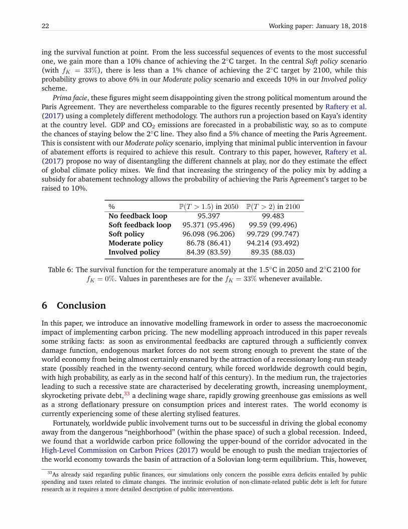
22 Working paper: January 18, 2018
ing the survival function at point. From the less successful sequences of events to the most successfulone, we gain more than a 10% chance of achieving the 2◦C target. In the central Soft policy scenario(with fK = 33%), there is less than a 1% chance of achieving the 2◦C target by 2100, while thisprobability grows to above 6% in our Moderate policy scenario and exceeds 10% in our Involved policyscheme.
Prima facie, these figures might seem disappointing given the strong political momentum around theParis Agreement. They are nevertheless comparable to the figures recently presented by Raftery et al.(2017) using a completely different methodology. The authors run a projection based on Kaya’s identityat the country level. GDP and CO2 emissions are forecasted in a probabilistic way, so as to computethe chances of staying below the 2◦C line. They also find a 5% chance of meeting the Paris Agreement.This is consistent with our Moderate policy scenario, implying that minimal public intervention in favourof abatement efforts is required to achieve this result. Contrary to this paper, however, Raftery et al.(2017) propose no way of disentangling the different channels at play, nor do they estimate the effectof global climate policy mixes. We find that increasing the stringency of the policy mix by adding asubsidy for abatement technology allows the probability of achieving the Paris Agreement’s target to beraised to 10%.
% P(T > 1.5) in 2050 P(T > 2) in 2100
No feedback loop 95.397 99.483Soft feedback loop 95.371 (95.496) 99.59 (99.496)Soft policy 96.098 (96.206) 99.729 (99.747)Moderate policy 86.78 (86.41) 94.214 (93.492)Involved policy 84.39 (83.59) 89.35 (88.03)
Table 6: The survival function for the temperature anomaly at the 1.5◦C in 2050 and 2◦C 2100 forfK = 0%. Values in parentheses are for the fK = 33% whenever available.
6 Conclusion
In this paper, we introduce an innovative modelling framework in order to assess the macroeconomicimpact of implementing carbon pricing. The new modelling approach introduced in this paper revealssome striking facts: as soon as environmental feedbacks are captured through a sufficiently convexdamage function, endogenous market forces do not seem strong enough to prevent the state of theworld economy from being almost certainly ensnared by the attraction of a recessionary long-run steadystate (possibly reached in the twenty-second century, while forced worldwide degrowth could begin,with high probability, as early as in the second half of this century). In the medium run, the trajectoriesleading to such a recessive state are characterised by decelerating growth, increasing unemployment,skyrocketing private debt,33 a declining wage share, rapidly growing greenhouse gas emissions as wellas a strong deflationary pressure on consumption prices and interest rates. The world economy iscurrently experiencing some of these alerting stylised features.
Fortunately, worldwide public involvement turns out to be successful in driving the global economyaway from the dangerous “neighborhood” (within the phase space) of such a global recession. Indeed,we found that a worldwide carbon price following the upper-bound of the corridor advocated in theHigh-Level Commission on Carbon Prices (2017) would be enough to push the median trajectories ofthe world economy towards the basin of attraction of a Solovian long-term equilibrium. This, however,
33As already said regarding public finances, our simulations only concern the possible extra deficits entailed by publicspending and taxes related to climate changes. The intrinsic evolution of non-climate-related public debt is left for futureresearch as it requires a more detailed description of public interventions.
Carbon Pricing and Global Warming: A Stock-flow Consistent Macro-dynamic Approach 23
is compatible with the two following features: first, some worst-case distribution tails of our simula-tions, where high levels of private non-financial debt are possibly reached and, second, some medium-run trade-off in terms of lower real income growth and higher non-financial indebtedness.. However,the economy appears to be better-off at the end of the century due to the containment of climate dam-ages. Moreover, prudent climate risk management suggests the need to ask for additional policy tools:in this paper, we show that, whenever abatement costs are sufficiently subsidised in addition to theimplementation of some carbon pricing, even the worst-case distribution tails of our simulations seemto become viable.
This paper calls for a number of extensions that have already been partly suggested throughout thepaper.34 Firstly, designing the financial system is a key challenge to elucidate its complex interactionwith the consequences of climate change (Jackson et al., 2014). We view our paper as a first attempt totackle this issue. A more detailed description of the prudential rules followed by the banking sector (e.g.following Giraud and Kockerols (2015)), or introducing endogenous default and collateral constraints(e.g. following Geanakoplos and Zame (2014)) would make it possible not only to better understandcredit rationing but also to propose some recommendations for macro-prudential regulation. Further-more, numerous scholars have pointed out the key issue linking climate change and inequality (IPCC,2014; Jackson et al., 2014). In this paper, inequality has only been dealt with in terms of the classicaltrade-off between capital return and wages: as climate destruction seems to boost the share of capi-tal within an otherwise possibly decelerating (or even declining) world income, the higher the wageshare, the more resilient the economy. A deeper grasp of the issue at stake could obviously be obtainedby disaggregating households (e.g. following Giraud and Grasselli (2017), who suggest, without cli-mate considerations, that reducing inequality may foster growth under some specific circumstances).Moreover, our system dynamical approach is well suited to dealing with other key issues related to theenergy shift, such as the depletion of fossil fuels and mineral stocks:35 Capturing how the latter canfeed back to affect economic performances would have considerable consequences for policymakingand will be considered in future research. Lastly and most importantly, there is a need to explore otherpublic policy instruments, such as subsidies for green capital specifically or differentiated interest ratesfor loans to stimulate green investments. These might lower the burden of the carbon tax on the privatesector and ease the transition towards a low-carbon economy.
Acknowledgements
We thank the participants of the academic symposium held on May 2017 at Ecole Normale Superieure,Paris, co-hosted by the World Bank and the Agence Francaise de Developpement (AFD), for useful com-ments. All remaining errors are our own. This work benefited from the support of the Energy and Pros-perity Chair and the financial support of the Agence Nationale de la Recherche (project MeET-MaDyS).
Appendices
A Reduced-form
The climate-economy interplay in our model can be wrapped up through a simple reduced-form. Giventhe trajectories of the climate-side of the model, namely (DY,DK, A, T, pc, pBS), the dynamical system
34E.g., in Footnotes 10, 11, 14, 15 and 33.35A Lotka-Volterra perspective proved useful, e.g., in the fish-stock model by Cordier et al. (2017). On the other hand, Vidal
et al. (2017) have shown that a number of minerals—first and foremost, copper—will presumably reach their extraction peakat a planetary scale in the coming decades.
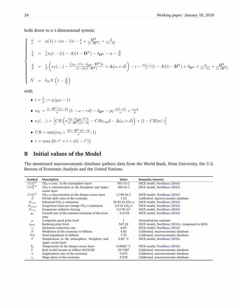
24 Working paper: January 18, 2018
boils down to a 4-dimensional system:
ωω = φ(λ) + (m− 1)i− a
a + DY
(1−DY)+ A
(1−A)
λλ = 1
νκI(· · · )(1−A)(1−DY)− δDK − α− NN
dd = 1
d
(κI(. . .)−
(πK−CP−δDK−DK)ν(1−A)(1−DY)
+ ∆(ω, r, d)
)− i− κI(...)
ν (1−A)(1−DY) + δDK + A(1−A) + DY
(1−DY)
N = δNN(
1− NN
)with
• i = pp := η (µω − 1)
• πK = (1−DY)(1−A)ν (1− ω − rd)− δDK − pC σ(1−n)
ν + sAAν
• κI(. . .) =[CR
(νπK+δ
DK+CP(1−DY)(1−A)
− CRsrepd−∆(ω, r, d))
+ (1− CR)κ(·)]
• CR = min(cr0 + d(1−DY)(1−A)ν , 1)
• r = max {0, r∗ + i+ φ(i− i∗)}
B Initial values of the Model
The mentioned macroeconomic database gathers data from the World Bank, Penn University, the U.S.Bureau of Economic Analysis and the United Nations.
Symbol Description Value Remarks/sourcesCOAT2 CO2-e conc. in the atmosphere layer 851 Gt C DICE model, Nordhaus (2016)COUP2 CO2-e concentration in the biosphere and upper
ocean layer460 Gt C DICE model, Nordhaus (2016)
COLO2 CO2-e concentration in the deeper ocean layer 1,740 Gt C DICE model, Nordhaus (2016)d Private debt ratio of the economy 1.53 Calibrated, macroeconomic database
Eind Industrial CO2-e emissions 35.85 Gt CO2-e DICE model, Nordhaus (2016)Eland Exogenous land-use change CO2-e emissions 2.6 Gt CO2-e DICE model, Nordhaus (2016)Fexo Exogenous radiative forcing 0.5 W/m2 DICE model, Nordhaus (2016)gσ Growth rate of the emission intensity of the econ-
omy- 0.0152 DICE model, Nordhaus (2016)
p Composite good price level 1 Normalization constantpBS Backstop price level 547.22 DICE model, Nordhaus (2016), compound to 2016n Emissions reduction rate 0.03 DICE model, Nordhaus (2016)N Workforce of the economy in billions 4.83 Calibrated, macroeconomic databaseNG Total population in billions 7.35 Calibrated, macroeconomic databaseT Temperature in the atmosphere, biosphere and
upper ocean layer0.85 ◦C DICE model, Nordhaus (2016)
T0 Temperature in the deeper ocean layer 0.0068 ◦C DICE model, Nordhaus (2016)Y Real world income in trillion 2015US$ 59.7387 Calibrated, macroeconomic databaseλ Employment rate of the economy 0.675 Calibrated, macroeconomic databaseω Wage share of the economy 0.578 Calibrated, macroeconomic database
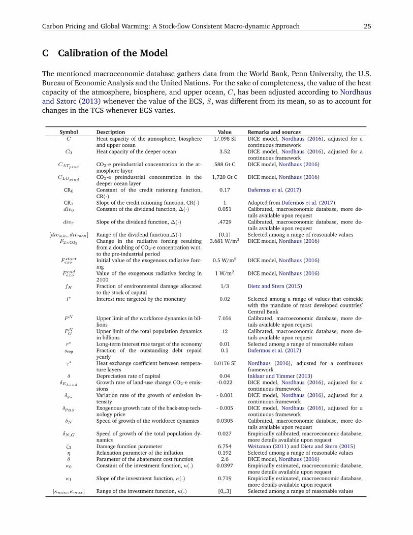
Carbon Pricing and Global Warming: A Stock-flow Consistent Macro-dynamic Approach 25
C Calibration of the Model
The mentioned macroeconomic database gathers data from the World Bank, Penn University, the U.S.Bureau of Economic Analysis and the United Nations. For the sake of completeness, the value of the heatcapacity of the atmosphere, biosphere, and upper ocean, C, has been adjusted according to Nordhausand Sztorc (2013) whenever the value of the ECS, S, was different from its mean, so as to account forchanges in the TCS whenever ECS varies.
Symbol Description Value Remarks and sourcesC Heat capacity of the atmosphere, biosphere
and upper ocean1/.098 SI DICE model, Nordhaus (2016), adjusted for a
continuous frameworkC0 Heat capacity of the deeper ocean 3.52 DICE model, Nordhaus (2016), adjusted for a
continuous frameworkCATpind CO2-e preindustrial concentration in the at-
mosphere layer588 Gt C DICE model, Nordhaus (2016)
CLOpind CO2-e preindustrial concentration in thedeeper ocean layer
1,720 Gt C DICE model, Nordhaus (2016)
CR0 Constant of the credit rationing function,CR(·)
0.17 Dafermos et al. (2017)
CR1 Slope of the credit rationing function, CR(·) 1 Adapted from Dafermos et al. (2017)div0 Constant of the dividend function, ∆(·) 0.051 Calibrated, macroeconomic database, more de-
tails available upon requestdivπ Slope of the dividend function, ∆(·) .4729 Calibrated, macroeconomic database, more de-
tails available upon request[divmin, divmax] Range of the dividend function,∆(·) [0,1] Selected among a range of reasonable values
F2×CO2Change in the radiative forcing resultingfrom a doubling of CO2-e concentration w.r.t.to the pre-industrial period
3.681 W/m2 DICE model, Nordhaus (2016)
F startexo Initial value of the exogenous radiative forc-ing
0.5 W/m2 DICE model, Nordhaus (2016)
F endexo Value of the exogenous radiative forcing in2100
1 W/m2 DICE model, Nordhaus (2016)
fK Fraction of environmental damage allocatedto the stock of capital
1/3 Dietz and Stern (2015)
i∗ Interest rate targeted by the monetary 0.02 Selected among a range of values that coincidewith the mandate of most developed countries’Central Bank
PN Upper limit of the workforce dynamics in bil-lions
7.056 Calibrated, macroeconomic database, more de-tails available upon request
PNG Upper limit of the total population dynamicsin billions
12 Calibrated, macroeconomic database, more de-tails available upon request
r∗ Long-term interest rate target of the economy 0.01 Selected among a range of reasonable valuessrep Fraction of the outstanding debt repaid
yearly0.1 Dafermos et al. (2017)
γ∗ Heat exchange coefficient between tempera-ture layers
0.0176 SI Nordhaus (2016), adjusted for a continuousframework
δ Depreciation rate of capital 0.04 Inklaar and Timmer (2013)δELand Growth rate of land-use change CO2-e emis-
sions-0.022 DICE model, Nordhaus (2016), adjusted for a
continuous frameworkδgσ Variation rate of the growth of emission in-
tensity- 0.001 DICE model, Nordhaus (2016), adjusted for a
continuous frameworkδpBS Exogenous growth rate of the back-stop tech-
nology price- 0.005 DICE model, Nordhaus (2016), adjusted for a
continuous frameworkδN Speed of growth of the workforce dynamics 0.0305 Calibrated, macroeconomic database, more de-
tails available upon requestδN,G Speed of growth of the total population dy-
namics0.027 Empirically calibrated, macroeconomic database,
more details available upon requestζ3 Damage function parameter 6.754 Weitzman (2011) and Dietz and Stern (2015)η Relaxation parameter of the inflation 0.192 Selected among a range of reasonable valuesθ Parameter of the abatement cost function 2.6 DICE model, Nordhaus (2016)κ0 Constant of the investment function, κ(.) 0.0397 Empirically estimated, macroeconomic database,
more details available upon requestκ1 Slope of the investment function, κ(.) 0.719 Empirically estimated, macroeconomic database,
more details available upon request[κmin, κmax] Range of the investment function, κ(.) [0,.3] Selected among a range of reasonable values
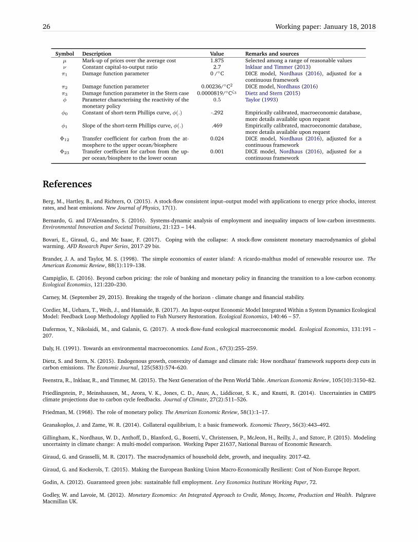
26 Working paper: January 18, 2018
Symbol Description Value Remarks and sourcesµ Mark-up of prices over the average cost 1.875 Selected among a range of reasonable valuesν Constant capital-to-output ratio 2.7 Inklaar and Timmer (2013)π1 Damage function parameter 0 /◦C DICE model, Nordhaus (2016), adjusted for a
continuous frameworkπ2 Damage function parameter 0.00236/◦C2 DICE model, Nordhaus (2016)π3 Damage function parameter in the Stern case 0.0000819/◦Cζ3 Dietz and Stern (2015)φ Parameter characterising the reactivity of the
monetary policy0.5 Taylor (1993)
φ0 Constant of short-term Phillips curve, φ(.) -.292 Empirically calibrated, macroeconomic database,more details available upon request
φ1 Slope of the short-term Phillips curve, φ(.) .469 Empirically calibrated, macroeconomic database,more details available upon request
Φ12 Transfer coefficient for carbon from the at-mosphere to the upper ocean/biosphere
0.024 DICE model, Nordhaus (2016), adjusted for acontinuous framework
Φ23 Transfer coefficient for carbon from the up-per ocean/biosphere to the lower ocean
0.001 DICE model, Nordhaus (2016), adjusted for acontinuous framework
References
Berg, M., Hartley, B., and Richters, O. (2015). A stock-flow consistent input–output model with applications to energy price shocks, interestrates, and heat emissions. New Journal of Physics, 17(1).
Bernardo, G. and D’Alessandro, S. (2016). Systems-dynamic analysis of employment and inequality impacts of low-carbon investments.Environmental Innovation and Societal Transitions, 21:123 – 144.
Bovari, E., Giraud, G., and Mc Isaac, F. (2017). Coping with the collapse: A stock-flow consistent monetary macrodynamics of globalwarming. AFD Research Paper Series, 2017-29 bis.
Brander, J. A. and Taylor, M. S. (1998). The simple economics of easter island: A ricardo-malthus model of renewable resource use. TheAmerican Economic Review, 88(1):119–138.
Campiglio, E. (2016). Beyond carbon pricing: the role of banking and monetary policy in financing the transition to a low-carbon economy.Ecological Economics, 121:220–230.
Carney, M. (September 29, 2015). Breaking the tragedy of the horizon - climate change and financial stability.
Cordier, M., Uehara, T., Weih, J., and Hamaide, B. (2017). An Input-output Economic Model Integrated Within a System Dynamics EcologicalModel: Feedback Loop Methodology Applied to Fish Nursery Restoration. Ecological Economics, 140:46 – 57.
Dafermos, Y., Nikolaidi, M., and Galanis, G. (2017). A stock-flow-fund ecological macroeconomic model. Ecological Economics, 131:191 –207.
Daly, H. (1991). Towards an environmental macroeconomics. Land Econ., 67(3):255–259.
Dietz, S. and Stern, N. (2015). Endogenous growth, convexity of damage and climate risk: How nordhaus’ framework supports deep cuts incarbon emissions. The Economic Journal, 125(583):574–620.
Feenstra, R., Inklaar, R., and Timmer, M. (2015). The Next Generation of the Penn World Table. American Economic Review, 105(10):3150–82.
Friedlingstein, P., Meinshausen, M., Arora, V. K., Jones, C. D., Anav, A., Liddicoat, S. K., and Knutti, R. (2014). Uncertainties in CMIP5climate projections due to carbon cycle feedbacks. Journal of Climate, 27(2):511–526.
Friedman, M. (1968). The role of monetary policy. The American Economic Review, 58(1):1–17.
Geanakoplos, J. and Zame, W. R. (2014). Collateral equilibrium, I: a basic framework. Economic Theory, 56(3):443–492.
Gillingham, K., Nordhaus, W. D., Anthoff, D., Blanford, G., Bosetti, V., Christensen, P., McJeon, H., Reilly, J., and Sztorc, P. (2015). Modelinguncertainty in climate change: A multi-model comparison. Working Paper 21637, National Bureau of Economic Research.
Giraud, G. and Grasselli, M. R. (2017). The macrodynamics of household debt, growth, and inequality. 2017-42.
Giraud, G. and Kockerols, T. (2015). Making the European Banking Union Macro-Economically Resilient: Cost of Non-Europe Report.
Godin, A. (2012). Guaranteed green jobs: sustainable full employment. Levy Economics Institute Working Paper, 72.
Godley, W. and Lavoie, M. (2012). Monetary Economics: An Integrated Approach to Credit, Money, Income, Production and Wealth. PalgraveMacmillan UK.
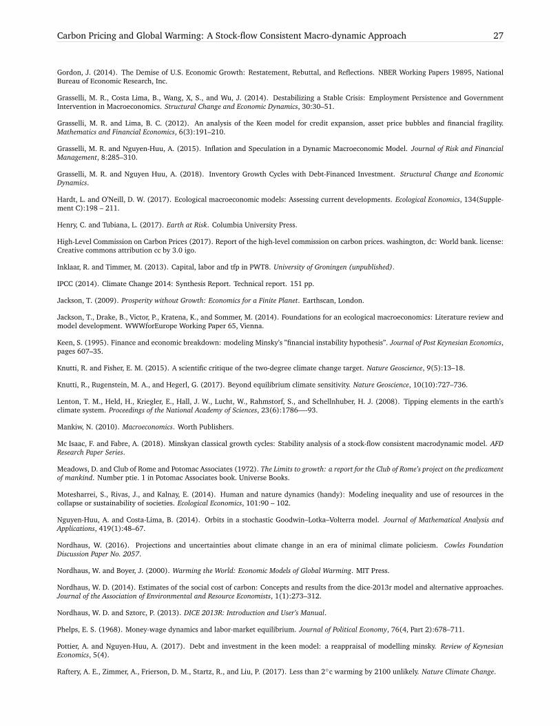
Carbon Pricing and Global Warming: A Stock-flow Consistent Macro-dynamic Approach 27
Gordon, J. (2014). The Demise of U.S. Economic Growth: Restatement, Rebuttal, and Reflections. NBER Working Papers 19895, NationalBureau of Economic Research, Inc.
Grasselli, M. R., Costa Lima, B., Wang, X, S., and Wu, J. (2014). Destabilizing a Stable Crisis: Employment Persistence and GovernmentIntervention in Macroeconomics. Structural Change and Economic Dynamics, 30:30–51.
Grasselli, M. R. and Lima, B. C. (2012). An analysis of the Keen model for credit expansion, asset price bubbles and financial fragility.Mathematics and Financial Economics, 6(3):191–210.
Grasselli, M. R. and Nguyen-Huu, A. (2015). Inflation and Speculation in a Dynamic Macroeconomic Model. Journal of Risk and FinancialManagement, 8:285–310.
Grasselli, M. R. and Nguyen Huu, A. (2018). Inventory Growth Cycles with Debt-Financed Investment. Structural Change and EconomicDynamics.
Hardt, L. and O’Neill, D. W. (2017). Ecological macroeconomic models: Assessing current developments. Ecological Economics, 134(Supple-ment C):198 – 211.
Henry, C. and Tubiana, L. (2017). Earth at Risk. Columbia University Press.
High-Level Commission on Carbon Prices (2017). Report of the high-level commission on carbon prices. washington, dc: World bank. license:Creative commons attribution cc by 3.0 igo.
Inklaar, R. and Timmer, M. (2013). Capital, labor and tfp in PWT8. University of Groningen (unpublished).
IPCC (2014). Climate Change 2014: Synthesis Report. Technical report. 151 pp.
Jackson, T. (2009). Prosperity without Growth: Economics for a Finite Planet. Earthscan, London.
Jackson, T., Drake, B., Victor, P., Kratena, K., and Sommer, M. (2014). Foundations for an ecological macroeconomics: Literature review andmodel development. WWWforEurope Working Paper 65, Vienna.
Keen, S. (1995). Finance and economic breakdown: modeling Minsky’s ”financial instability hypothesis”. Journal of Post Keynesian Economics,pages 607–35.
Knutti, R. and Fisher, E. M. (2015). A scientific critique of the two-degree climate change target. Nature Geoscience, 9(5):13–18.
Knutti, R., Rugenstein, M. A., and Hegerl, G. (2017). Beyond equilibrium climate sensitivity. Nature Geoscience, 10(10):727–736.
Lenton, T. M., Held, H., Kriegler, E., Hall, J. W., Lucht, W., Rahmstorf, S., and Schellnhuber, H. J. (2008). Tipping elements in the earth’sclimate system. Proceedings of the National Academy of Sciences, 23(6):1786—-93.
Mankiw, N. (2010). Macroeconomics. Worth Publishers.
Mc Isaac, F. and Fabre, A. (2018). Minskyan classical growth cycles: Stability analysis of a stock-flow consistent macrodynamic model. AFDResearch Paper Series.
Meadows, D. and Club of Rome and Potomac Associates (1972). The Limits to growth: a report for the Club of Rome’s project on the predicamentof mankind. Number ptie. 1 in Potomac Associates book. Universe Books.
Motesharrei, S., Rivas, J., and Kalnay, E. (2014). Human and nature dynamics (handy): Modeling inequality and use of resources in thecollapse or sustainability of societies. Ecological Economics, 101:90 – 102.
Nguyen-Huu, A. and Costa-Lima, B. (2014). Orbits in a stochastic Goodwin–Lotka–Volterra model. Journal of Mathematical Analysis andApplications, 419(1):48–67.
Nordhaus, W. (2016). Projections and uncertainties about climate change in an era of minimal climate policiesm. Cowles FoundationDiscussion Paper No. 2057.
Nordhaus, W. and Boyer, J. (2000). Warming the World: Economic Models of Global Warming. MIT Press.
Nordhaus, W. D. (2014). Estimates of the social cost of carbon: Concepts and results from the dice-2013r model and alternative approaches.Journal of the Association of Environmental and Resource Economists, 1(1):273–312.
Nordhaus, W. D. and Sztorc, P. (2013). DICE 2013R: Introduction and User’s Manual.
Phelps, E. S. (1968). Money-wage dynamics and labor-market equilibrium. Journal of Political Economy, 76(4, Part 2):678–711.
Pottier, A. and Nguyen-Huu, A. (2017). Debt and investment in the keen model: a reappraisal of modelling minsky. Review of KeynesianEconomics, 5(4).
Raftery, A. E., Zimmer, A., Frierson, D. M., Startz, R., and Liu, P. (2017). Less than 2◦c warming by 2100 unlikely. Nature Climate Change.
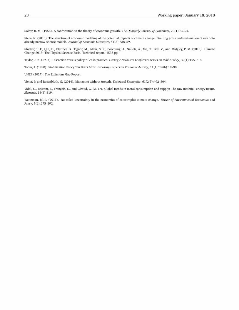
28 Working paper: January 18, 2018
Solow, R. M. (1956). A contribution to the theory of economic growth. The Quarterly Journal of Economics, 70(1):65–94.
Stern, N. (2013). The structure of economic modeling of the potential impacts of climate change: Grafting gross underestimation of risk ontoalready narrow science models. Journal of Economic Literature, 51(3):838–59.
Stocker, T. F., Qin, D., Plattner, G., Tignor, M., Allen, S. K., Boschung, J., Nauels, A., Xia, Y., Bex, V., and Midgley, P. M. (2013). ClimateChange 2013: The Physical Science Basis. Technical report. 1535 pp.
Taylor, J. B. (1993). Discretion versus policy rules in practice. Carnegie-Rochester Conference Series on Public Policy, 39(1):195–214.
Tobin, J. (1980). Stabilization Policy Ten Years After. Brookings Papers on Economic Activity, 11(1, Tenth):19–90.
UNEP (2017). The Emissions Gap Report.
Victor, P. and Rosenbluth, G. (2014). Managing without growth. Ecological Economics, 61(2-3):492–504.
Vidal, O., Rostom, F., Francois, C., and Giraud, G. (2017). Global trends in metal consumption and supply: The raw material–energy nexus.Elements, 13(5):319.
Weitzman, M. L. (2011). Fat-tailed uncertainty in the economics of catastrophic climate change. Review of Environmental Economics andPolicy, 5(2):275–292.
List of recent AFD Research Papers
AFD Research Papers are available through AFD’s website at http://editions.afd.fr
# 2017-53 SIMONNEAU, C. and Irène SALENSON (2017), “Holding Land in Common within Cities: What Can We Learn from Collective Tenure in Urban Context?”, AFD Research Papers Series, n° 2017-53, September.
# 2017-54 CAMPIGLIO, E., GODIN A., KEMP-BENEDICT, E. (2017), “Networks of stranded assets: A case for a balance sheet approach”, AFD Research Papers, No. 2017-54, October.
# 2017-55 DAO, T.H., F. DOCQUIER, M. MAUREL and P. SCHAUS (2017), “Global Migration in the 20th and 21st Centuries: the Unstoppable Force of Demography ”, AFD Research Paper Series, No. 2017-55, November.
# 2017-56 SHAPIRO, D., “Linkages between Education and Fertility in Sub-Saharan Africa”, AFD Research Paper Series, No. 2017-56, November.
# 2017-57 SCHUYT, T., HOOLWERF, L.K. and D. VERKAIK (2017), “Better together? A Study on Philanthropy and Official Development Assistance”, AFD Research Papers Series, No. 2017-57, February.
# 2017-59 EL-DALY, M. and M. KHALIL (2017), “Philanthropy in the Arab World”, AFD Research Papers Series, No. 2017-59, October.
# 2017-60 BOVARI, E., O. LECUYER, F. Mc ISAAC (2017), “Debt and damages: what are the chances of staying under the 2°C warming threshold?”, AFD Research Papers Series, No. 2017-60, November.
# 2017-61 BOVARI Mc ISAAC, F. (2017), “Testing Goodwin with a Stochastic Differential Approach–The United States (1948-2017)”, AFD Research Papers Series, No. 2017-61, November.
# 2017-62 Mc ISAAC, F., D. BASTIDAS (2017), “An Input-Output Analysis: What Would a Low-Carbon Economy for Brazil Mean?”, AFD Research Papers Series, No. 2017-62, December.
# 2017-63 DAVID, A., GUILBERT, N., HINO, H., LEIBBRANDT, M., POTGIETER, E. and M. SHIFA (2018), “Social Cohesion and inequality in South Africa”, AFD Research Papers Series, No. 2017-63.
# 2018-64 DE BERCEGOL, R., J. CAVÉ and A. NGUYEN THAI HUYEN (2018), “Informal Recycling vs municipal Waste Service in Asian cities: Opposition or Integration?”, AFD Research Papers Series, No. 2018-64