Research Paper 37 | 2015

CHASING AFTER THE FRONTIER IN AGRICULTURAL PRODUCTIVITY Jules-Daniel WURLOD, Derek EATON

Chasing After the Frontier in Agricultural Productivity

Jules-Daniel Wurlod∗ Derek Eaton††

November 2015

Abstract

This paper explores international productivity patterns in agriculture. We test whether

countries higher productivity growth has been experienced by countries that were initially

further from the technological frontier. Based on a panel of 84 countries at various levels of

development, we find support for convergence among OECD countries but divergence in our

sample at large over the period 1960-2010. We then test whether technological catch-up is

conditional on absorptive capacities and domestic investments in R&D. While agricultural re-

search intensity has a significant effect on labor productivity growth, the size of this effect

decreases the further the country is from the frontier. We calculate a threshold level for the

effectiveness of research intensity: increased R&D contributes to catching up to the frontier for

those countries with a distance to the frontier less than 22. We also test for additional factors

affecting productivity growth, and find that secondary education plays a strong role in less de-

veloped countries, while trade openness appears to have had a positive effect on productivity

in middle income countries. On the other hand, there is little evidence of much effect, either

positive or negative from IPR protection. Of perhaps greater interest is the apparent impact of

economic growth outside of agriculture in driving agricultural productivity improvements.

Keywords: agriculture, productivity, convergence, R&D, IPR, education.

JEL classification: O13, O33, Q11, Q16, Q18.

∗Corresponding author. Graduate Institute of International and Development Studies and Centre for InternationalEnvironmental Studies, Switzerland. E-mail: jules-daniel.wurlod@graduateinstitute.ch. Tel: +41/79.664.53.27.†Graduate Institute of International and Development Studies and Centre for International Environmental Studies,

Switzerland.The research leading to these results has received funding from the European Union’s Seventh Framework ProgrammeFP7/2007-2011 under Grant Agreement no. 290693 FOODSECURE. The authors only are responsible for any omissionsor deficiencies. Neither the FOODSECURE project and any of its partner organizations, nor any organization of theEuropean Union or European Commission are accountable for the content of papers.

1 Introduction

Productivity growth in agriculture has recently been of renewed concern from a food security

perspective. First, while productivity growth has historically been high in developing nations

since World War II, the rate of increase of productivity improvements appears to have slowed

while demand for food and agricultural products is expected to continue growing (Pardey et al.,

2013, 2014). Secondly, sustainability concerns imply that agricultural production needs to be

increased on existing agricultural lands, to halt further conversion of natural lands. Thirdly,

episodes of food price volatility in the first decade of this century posed challenges to how de-

veloping economies dependent on food imports can ensure affordable access to foodstuffs. Main-

taining and enhancing productivity growth in agriculture, particularly among countries that are

currently much less productive, is therefore an urgent policy matter (Alston and Pardey, 2014).

There are two sources of productivity growth: technical change, or movement of the technol-

ogy frontier, and a catch-up effect, or efficiency change, whenever countries are moving closer to

the frontier. A longstanding conjecture in growth theory is that countries with less productive

technologies can catch-up with frontier countries by leapfrogging on early stages of technological

development, affording them with higher productivity growth (important contributions include

Gerschenkron, 1962; Barro and Sala-i Martin, 1997; Howitt, 2000; Acemoglu and Zilibotti, 2001).

Furthermore, simply by assuming some form of public good nature of knowledge, productivity

convergence becomes a natural outcome, with economies further behind the frontier tending to

grow faster (Fare et al., 1994; Abramovitz, 1990). However, technology diffusion might not be

automatic, and there might also be conditions necessary in order to benefit from the advantage of

‘backwardness’. Nelson and Phelps (1966), and more recently Benhabib and Spiegel (1994) and

Islam et al. (2014), have highlighted that absorptive capacities, determined primarily by human

capital, might be a condition for the transfer of technologies. This is distinct from the primary role

of human capital in technological change that is acknowledged in modern endogenous growth

models (see for example Howitt, 2000; Acemoglu and Zilibotti, 2001).

As emphasized by Pardey et al. (2010), the agricultural sector presents specific characteris-

tics and circumstances that could impact the likelihood of technology diffusion to less productive

economies. First, production units in agriculture are generally quite numerous and atomistic,

which can slow or complicate the process of technology adoption in primary production, partic-

ularly for multi-faceted technologies combining a range of inputs with tacit knowledge. Second,

uncontrolled factors, such as agricultural pests, and changing weather and climatic conditions,

1

require investments in maintenance research to prevent the erosion of past productivity gains.

More importantly, technologies developed in a given agro-ecological and socioeconomic context

may not necessarily suitable in others without some form of adaptation (Eberhardt and Teal, 2012).

This could imply that technology transfer in agriculture is conditional on domestic R&D invest-

ments to adapt inputs (e.g. seeds, machinery, chemicals) and production techniques to local speci-

ficities (Pardey et al., 2010).

In terms of empirics, several studies have tested the convergence hypothesis for total factor

productivity (TFP) in agriculture. Martin and Mitra (2001) found that technology catch-up occurs

faster in agriculture than in the manufacturing sector, using a sample of 50 countries at differ-

ent stages of development from 1967 to 1992. In contrast Suhariyanto and Thirtle (2001) find

no evidence of convergence in agriculture among 18 Asian countries over the period 1965-1996.

Schimmelpfennig and Thirtle (1999), as well as Rezitis (2010), find mixed evidence of productivity

convergence in agriculture between the United States and European countries using time series

tests. Rao and Coelli (2004) and Coelli and Rao (2005) have shown partial evidence of TFP conver-

gence: countries that were less efficient in 1980 have a higher TFP growth rate than countries that

were at the frontier in 1980, and conclude that these results indicate both a degree of catch-up due

to improved technical efficiency along with technical change at the frontier. Ludena et al. (2007)

have found that the frontier in agriculture advanced more rapidly over 1960–1970s than individ-

ual TFP, thereby leading to divergence, or negative technical efficiency growth, but convergence,

or catching up to frontier, in the 1980–1990s.

More recent evidence, such as that of Fuglie et al. (2012), points towards robust but highly

uneven productivity growth in agriculture across countries. One argument for these differences

might be investments in research and development. Although the empirical literature on the ben-

efits from R&D at the macro level is limited and fragmentary (Pingali and Heisey, 1999), evidence

seems to point towards a statistically significant impact (for example Pardey and Beintema, 2001;

Alene, 2010; Fuglie et al., 2012), though much smaller than suggested by the micro ‘case-study’

literature.1 Other authors come to less equivocal conclusions. Wang et al. (2013) find that R&D

1The rates of return of R&D measured in the micro case-study literature can be very skewed, but are usually high:the mean and the mode of all studies combined are respectively 81 and 44 percent (Alston et al., 2000). The microliterature on the impact of R&D and innovation on agricultural productivity emerged in the 1960’s. The first paperto add R&D in a production function approach to measure its impact on productivity is Griliches (1964). Since then,numerous contributions have been made – around 300 studies – a third published in peer-reviewed journals (see Alston,2010, for a complete review of these studies). In all cases, heterogeneity in estimates on the productivity effect of R&Dcan be caused by modeling challenges, arising because benefits are spread both across economic agents and throughtime. These are identified in the literature as ‘temporal’ and ‘spatial’ attribution problems (Alston, 2010). Temporalattribution problems are caused by the time lag between costs and benefits, a sum of the ‘gestation’ or ‘invention’ lag(the time required to develop new technologies), and the ‘adoption’ lag, the time required for the technology to reach

2

affects agricultural productivity only over the long term, as only research stocks, or accumula-

tion of several years of expenditure, have a statistically significant impact on agricultural TFP

growth. In a study including both absorptive capacities (education/extension) and capacities of

scientists to innovate and adapt foreign technologies in a single econometric framework, Evenson

and Fuglie (2010) find that marginal increases in technology capital, given minimum levels of ed-

ucation and/or extension, have an impact on productivity growth. On the other hand, marginal

increases in education and/or extension, even given miminum levels of technology capital, do not

seem to have much impact.

One contribution of our paper is to re-examine the convergence hypothesis (as formulated by

Nelson and Phelps (1966) and Howitt (2000)) in the case of the agricultural sector over a longer

timeframe and using panel data techniques. We use the cross-country dataset of inputs, outputs

and productivity measures over 1960-2010 developed by Fuglie (2012), starting from FAOSTAT

but with adjustments for differences in input quality. After first testing whether the unconditional

convergence hypotheses holds for the agricultural sector, we test whether convergence occurs

conditional on investments in R&D and on absorptive capacities. We combine data on R&D ex-

penses for both OECD and developing countries from various sources, and follow an empirical

framework and specification recently suggested by Madsen et al. (2010) for aggregate productivity

growth (including manufacturing and services). In contrast with Evenson and Fuglie (2010), who

use two discrete composite indexes of invention-innovation and technology mastery, we use a

continuous variable for R&D expenditure, as well as for education. There are advantages and dis-

advantages to each approach which should probably be viewed as complementary to each other.

Our approach allows us to assess the effects of marginal changes in R&D and other variables,

without making assumptions about thresholds or cutoffs. But the dataset is not large enough to

allow us to explore such features with, for example, semiparametric techniques. The panel data

approach does allow us to control for country-specific unobservable factors through the inclu-

sion of country fixed effects, so far absent in most of the studies measuring productivity growth

rates in agriculture (see for example Headey et al., 2010). We also consider the issue of temporal

attribution problems by varying the number of lags in our estimates.

Our results suggest that research intensity has a positive impact on productivity growth in

all income groups, with the exception of LDCs. Furthermore, we find that the observed effect is

lower the further a country is behind the technological frontier. In other words, R&D seems to

farmers in the field (Pardey et al., 2010). The spatial attribution problem is due to the non-excludable and non-rivalnature of technology, as the number of agents benefitting from technological improvements can be large, making itharder to identify the range and to account for other factors. (Alston, 2010).

3

be more effective in more productive countries, in contrast with the general predictions from the

macroeconomic literature on productivity convergence. Overall, our findings suggest a more nu-

anced picture of the productivity impacts of R&D than usually found in the literature (for example

in Pardey et al., 2013). We do not conclude that R&D necessarily should be less effective but offer

possible explanations for this observed result in our discussion. In addition, our estimates of the

impact of education are also differentiated by income level: education appears to be more impor-

tant for enhancing agricultural productivity growth in less developed countries than for lower

and upper middle income countries (UMI/LMI).

In a second step, in light of the findings of heterogeneity across countries and income groups,

we test for additional determinants of productivity growth by sequentially incorporating vari-

ous regressors in a fixed effects model, building on the earlier work of Headey et al. (2010).2

We include policy and institutional factors found to affect productivity growth in the literature.

Specifically, we measure the impact of 1) trade openness, as in Madsen et al. (2010): increased

trade openness is expected to facilitate the inflow of foreign technologies; 2) intellectual property

rights, which can stimulate or hinder technological change and diffusion (Evenson and Swanson,

2010); 3) rural infrastructure and road density, potentially reducing transport costs and support-

ing market integration; 4) support to the agricultural sector, which can distort relative prices and

stimulates less efficient use of resources (Headey et al., 2010); 5) growth in non-agricultural sec-

tors, elaborating on recent findings by Lagakos and Waugh (2013) and Gollin et al. (2014) and 6)

civil conflicts, considering that many country/periods exhibit negative productivity growth rates.

We find that trade openness, IPR protection and economic growth in the non-agricultural sec-

tor have a statistically significant positive impact on productivity growth, and that these impacts

seem stronger for middle income countries than in LDCs. Civil conflicts are also found to have a

negative impact on productivity growth.

Our paper is structured as follows. In the next section, we describe the dataset used in our

study. Section 3 and 4 present some descriptive statistics on global patterns of productivity and

research intensity, while Section 5 describes our empirical specification. Sections 6 and 7 present

our main results, and Section 8 concludes.2A major difference though is that we use the productivity estimates of Fuglie (2012).

4

2 Data Sources

Data on inputs and outputs are from Fuglie (2012), published by the Economic Research Ser-

vice of the U.S. Department of Agriculture. This dataset includes yearly estimates of all major

input categories – labor, area harvested, machinery, fertilizers, livestock input and animal feed

consumption – for 170 countries at all income levels, from 1961 to 2010. The data originates from

FAOSTAT, and in some cases, is supplemented with data from national statistical sources. A major

advantage of this dataset is that some attempts are made to correct measures of various inputs for

differences in quality, which greatly improve productivity measurement (Craig et al., 1997). In the

case of land, for example, estimates are weighted by irrigation type, i.e. whether agricultural land

is rainfed, irrigated or used for pasture.3

In this paper, we choose to focus on labor productivity. First, because recent contributions

in the literature has shown that the measurement of cross-country TFP in agriculture presents

challenges in generating robust and plausible estimates in levels for cross-country comparisons

(Alston and Pardey, 2014), and that estimates of Total Factor Productivity (TFP) growth rates can

vary greatly with the methodology used. To illustrate this, Figure A1 in the Annex plots the

estimates for annual TFP growth rates from three major studies: Fuglie et al. (2012), Headey et al.

(2010) and Coelli and Rao (2005). Each study uses a different methodology to estimate TFP growth.

Fuglie et al. (2012) use a Solow decomposition method, Headey et al. (2010) use both a stochastic

frontier approach (SFA) and a data envelopment analysis (DEA), while Coelli and Rao (2005) use

a Malmquist index.4 In Figure A1, each point off the 45 degree line indicates a difference between

the TFP growth rates calculated by each study, for a given country in a given period.5 We see

3Our measures of inputs include: Labor: number of economically active persons in agriculture; livestock: numberof cattle-equivalent head of livestock on farms; machinery: number of 40-CV tractor-equivalent machinery units in use;fertilizers: Sum of N, P2O5, and K2O fertilizers in tons of ‘N-fertilizer equivalents’; animal feed consumption: Metricenergy-equivalents (1000 Mcal)

4From a methodological point of view, these are the 3 different families of models prevalent in the literature. Each ofthose methodologies have pros and cons. DEA consists in a linear optimization of combinations of inputs and outputs,with the advantage to remain a non-parametric approach, making results less sensitive to choices of functional forms.SFA models allow to account for the stochastic nature of production that can be caused by statistical noise, distinguish-ing between efficiency and the error term, but needs assumptions on a function functional form for production, suchas Cobb-Douglas or the more general translog production function, and needs assumptions on the distribution of theinefficiency parameters. Residual Approaches specify a production function and simply regress the value of output onthe different inputs. This approach suffers the same caveat as DEA methods, imputing distance from the productionfrontier strictly to differences in efficiency, without considering the stochastic dimension of agricultural production,and also needs an assumption on the functional form of the production function.

5Due to data aggregation issues, we can only compare studies providing growth rates for similar periods. Further-more, we need to aggregate annual growth rates into rates by decade. To this end, because the aggregation methodchosen might create self-generated differences, we use two alternative approaches. First, a simple arithmetic mean ofannual growth rates over the period under consideration. This methodology was chosen by Headey et al. (2010) toaggregate growth rates by decade. Second, we use a regression approach to estimate the growth rates out of the TFPlevels provided by the authors. The TFP growth rate over the period will be equal to the coefficient on a time trend

5

that the assessment of TFP growth rates in agriculture is not necessarily consistent across studies,

leaving significant room for improvement in further research, confirming the argument made by

Alston and Pardey (2014).

It is known that partial productivity measures have important shortcomings as proxies for

productivity. Using partial productivity measures at face value does not account for input substi-

tution (Capalbo and Antle, 1988). For example, if increased output per worker is obtained by an

increase in land use, despite the apparent impact on our partial productivity measure, TFP would

remain unchanged (Ludena et al., 2007). Although recent studies have shown that labor produc-

tivity and TFP growth tend to follow a similar pattern (see for example Madsen and Timol, 2011),

we control for input substitution by including other available inputs as control variables in all our

specifications, as in Dowrick and Nguyen (1989).

Our dataset for Research and Development comes from various sources. First, for developing

countries, we compile data from the Agricultural Science and Technology Indicators (ASTI) by

IFPRI, covering most low and middle income countries. To recover estimates of R&D expenditure

for previous periods, we rely on data from the ISNAR Agricultural Research Indicators Series,

edited by Pardey and Roseboom (1989), providing data on R&D expenditure based on surveys for

the period 1960–1986. For OECD countries, our main data source comes from Pardey et al. (1997)

for 1981 to 1993. For more recent periods, we complement our dataset with estimates from OECD

Stat, who provide gross domestic expenditure on R&D by sector of performance. Following the

literature (see for example Beintema and Stads, 2006), R&D expenses are normalized to account

for differences in the size of the agricultural sector. Because our production data does not provide

directly usable estimates of value added, we normalize our R&D figures by estimates of value

added by the World Development Indicators (WDI) of the World Bank. To measure education,

we use the Barro and Lee index of the average number of years of schooling of the population

over 25 years old (Barro and Lee, 2013). Section 7 requires additional data. The real rate of assis-

tance (RRA) data come from the "Database of Global Distortions to Agricultural Incentives" from

Anderson and Valenzuela (2008). Trade openness is measured as the sum of imports and exports

over GDP from WDI. Intellectual property rights data come from Ginarte and Park (Ginarte and

Park, 1997). Economic growth in the non-agricultural sectors are proxied by two variables. First

the non-agricultural GDP, calculated from agricultural and total GDP from WDI, and second the

percentage of rural population not employed in agriculture from FAOSTAT. Our road density net-

variable generated simply by regressing TFP levels on a constant and a time trend. For brevity purposes, only theresults using the arithmetic method are presented in the Annex, as results are not very sensitive to the aggregationmethod

6

(a) OECD (b) non-OECD

Figure 1: Labor Productivity Convergence

work estimates are borrowed from Calderon and Serven (2004). Finally, data for armed conflicts

come from UCPD (Gleditsch et al., 2002). We select only high intensity conflicts, i.e. conflicts

causing more than 1,000 deaths cumulatively.

3 Productivity Convergence

Figure 1 plots the initial distance to the frontier with the average productivity growth rate

throughout the rest of the sample period, for OECD and non-OECD income groups.6 Important

differences are evident. There seems to be convergence among OECD countries, where initially

less productive countries tend to grow faster, while this does not seem to be the case for non-OECD

countries. In other words, technology advances at the frontier seem to diffuse among OECD coun-

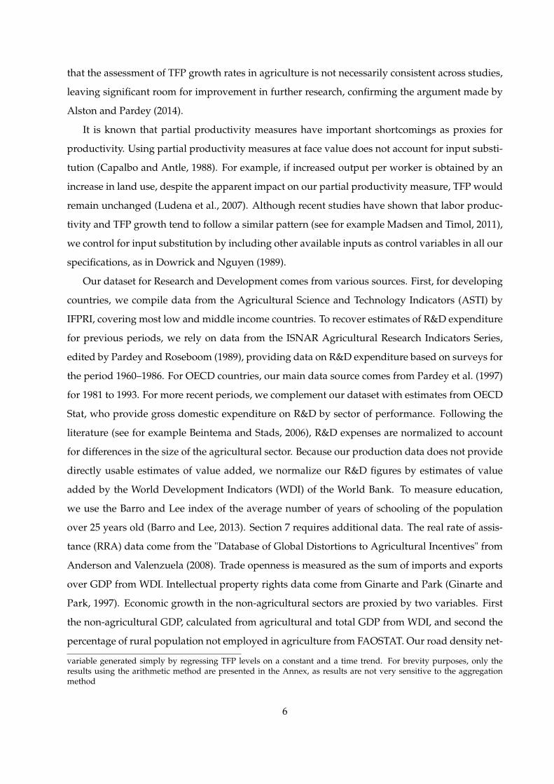
tries, but not to all countries in our sample. Figure 2 shows Box-whisker plots of the distribution

of distance to the frontier, by income level and through time. This allows to test the findings of

Ludena et al. (2007), who find divergence in TFP during the 1960s – 1970s and convergence during

the 1980s–1990s, as well as to differentiate between income groups. In case of convergence, the av-

erage distance to the frontier should decrease through time. As can be seen, the average distance

to the frontier decreased in the 1960s and 1970s for all income groups but LDCs, but, since the

1980s, it increased for all income groups but the OECD, suggesting that the agricultural sector in

middle- and low-income economies is lagging behind, with productivity growth rates below those

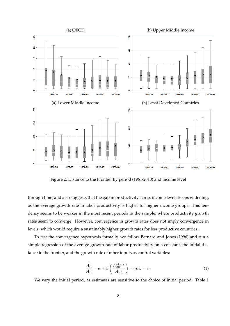
at the technological frontier. Figure 3 shows average productivity growth rates by income level6Income groups are defined using the World Bank definition for the year 1961. The list of countries and income

groups can be found in Table A1 in the Annex.

7

(a) OECD (b) Upper Middle Income

(a) Lower Middle Income (b) Least Developed Countries

Figure 2: Distance to the Frontier by period (1961-2010) and income level

through time, and also suggests that the gap in productivity across income levels keeps widening,

as the average growth rate in labor productivity is higher for higher income groups. This ten-

dency seems to be weaker in the most recent periods in the sample, where productivity growth

rates seem to converge. However, convergence in growth rates does not imply convergence in

levels, which would require a sustainably higher growth rates for less productive countries.

To test the convergence hypothesis formally, we follow Bernard and Jones (1996) and run a

simple regression of the average growth rate of labor productivity on a constant, the initial dis-

tance to the frontier, and the growth rate of other inputs as control variables:

Ait

Ait= α+ β

(AMAX

it0

Ait0

)+ γCit + εit (1)

We vary the initial period, as estimates are sensitive to the choice of initial period. Table 1

8

(a) OECD vs. non-OECD (b) By Income

Figure 3: Average Labor Productivity Growth

shows the estimated coefficients. Results confirm the patterns suggested graphically. For OECD

countries, the initial distance to the frontier is positively correlated with the growth rate in subse-

quent periods. However, when considering other income groups, or our sample as a whole, there

seems to be evidence of divergence in productivity. Overall, this section has shown that our data

does not seem to exhibit strong sign of convergence in productivity when taking our sample as a

whole, a result in contrast with the findings of Martin and Mitra (2001), Rao and Coelli (2004) and

Coelli and Rao (2005). The remaining of this study aims at measuring causes for (the absence of)

convergence for some income groups.

9

10

Tabl

e1:

Labo

rPr

oduc

tivi

tyC

onve

rgen

ce

(1a)

(1b)

(2a)

(2b)

(3a)

(3b)

(4a)

(4b)

(5a)

(5b)

1961

-65

1966

-70

1961

-65

1966

-70

1961

-65

1966

-70

1961

-65

1966

-70

1961

-65

1966

-70

Full

sam

ple

OEC

Dno

n-O

ECD

UM

I/LM

ILD

Cs

DTF

it0

-0.0

0681

***

-0.0

0678

***

0.01

15**

*0.

0112

**-0

.006

13**

*-0

.005

95**

*-0

.002

88-0

.004

45*

-0.0

0517

-0.0

0541

(0.0

00)

(0.0

00)

(0.0

02)

(0.0

37)

(0.0

01)

(0.0

01)

(0.2

84)

(0.0

86)

(0.3

75)

(0.3

10)

Land

g-0

.208

-0.2

070.

865*

0.69

9-0

.194

-0.2

07-0

.012

0-0

.052

90.

336

0.24

9(0

.183

)(0

.166

)(0

.071

)(0

.215

)(0

.226

)(0

.182

)(0

.953

)(0

.792

)(0

.205

)(0

.379

)Fe

rtg

0.00

568

0.02

440.

154

0.09

850.

0295

0.05

380.

0541

0.10

5**

0.01

820.

0281

(0.8

67)

(0.4

95)

(0.2

20)

(0.4

79)

(0.3

97)

(0.1

59)

(0.1

67)

(0.0

42)

(0.7

20)

(0.5

74)

Mac

hg0.

193*

**0.

219*

**-0

.187

-0.1

380.

153*

*0.

157*

*0.

0906

0.07

860.

0541

0.08

57(0

.000

)(0

.000

)(0

.104

)(0

.415

)(0

.012

)(0

.011

)(0

.248

)(0

.334

)(0

.491

)(0

.331

)Li

veg

0.18

8*0.

169

0.88

3***

0.74

6*0.

190*

0.17

6-0

.015

50.

0977

0.19

60.

276

(0.0

77)

(0.1

22)

(0.0

03)

(0.0

53)

(0.0

82)

(0.1

27)

(0.9

17)

(0.5

60)

(0.3

81)

(0.1

82)

Feed

g-0

.024

8-0

.043

4-0

.367

**-0

.300

0.00

471

-0.0

201

0.06

010.

0551

-0.0

241

-0.0

233

(0.6

64)

(0.4

59)

(0.0

28)

(0.1

58)

(0.9

35)

(0.7

40)

(0.4

11)

(0.4

66)

(0.7

54)

(0.7

99)

Cou

ntri

es12

412

424

2410

010

061

6128

28

Not

es:D

epen

dent

vari

able

:Ave

rage

labo

rpr

odgr

owth

,196

6-20

10fo

rsp

ec.(

a)an

d19

71-2

010

for

spec

.(b)

.p-v

alue

sin

pare

nthe

ses:

p***≤

0.01

,p**≤

0.05

,p*≤

0.1

(a) Total Expenses (b) R&D Intensity

Figure 4: R&D expenses and intensity, by income group, 1960–2010

Notes: Total expenses are in Mill. 2005 PPP $ and presented in 3-year moving average. R&D intensity is defined astotal expenses over agricultural GDP. Data for OECD countries for 1990–2010 available only for a subset of countries,and are therefore not presented to keep the sample unchanged

4 Research and Development

This section describes R&D expenses – both public and private – across countries and time.7

FIgure 4 shows R&D expenses and research intensity, as defined by total expenses over agricul-

tural GDP, averaged by income group. As can be seen, OECD countries still account for the major

share of world expenses in agricultural research and development. The average expenses for

middle income countries increased since the early 2000s, mostly pulled by China and India, to an

average annual of 600 million 2005 PPP $ per country. As a share of agricultural GDP, OECD coun-

tries are still leading, with annual expenses reaching almost 6% of GDP in the 90s. On average,

countries invest between 1–6% of agricultural GDP in research and development.8

Figure 5 shows Box-Whisker plots of intensities by decade and by income group. Furthermore,

even if the spread of observations is relatively high, the average intensity remains highest for

OECD countries. Furthermore, the average intensity in lower-middle income and low income

countries tends to decrease since 1990, whereas numbers for higher income groups tends to remain

stable or increase.

Table 2 shows the most and least productive countries, by period subsample, with their cor-

7For more comprehensive studies on patterns of R&D spendings, refer to Pardey et al. (2013), Beintema and Stads(2006) or Pardey et al. (2006).

8These figures are slightly higher than intensities reported in the literature, for example, in James et al. (2008).However, our dataset also includes private R&D spending, which accounts for almost half of total spendings in recentperiods in high income countries (Pardey et al., 2006)

11

(a) OECD (b) Upper Middle Income

(a) Lower Middle Income (b) Least Developed Countries

Figure 5: R&D expenses and intensity, by income group, 1960–2010

Notes: Total expenses are in Mill. 2005 PPP $ and presented in 3-year moving average. R&D intensity is defined astotal expenses over agricultural GDP

responding growth rate in productivity and their R&D expenses. From 1961 to 1980, the most

productive country was New Zealand, a country well endowed in land. Since 1980, the most pro-

ductive country is the US. The sample of most productive countries includes a range of countries

who all belong to the OECD income group.

On the other side of the spectrum, least productive countries are mostly SSA countries, but

also Vietnam during the war, Cambodia and Nepal. For these countries, the productivity growth

rates are on average lower than growth rates at the frontier, in contrast with predictions from the

convergence literature. Many countries/periods also present negative productivity growth.

One advantage of our dataset is to allow for a continuous measure of R&D expenses and

intensities. In contrast with Evenson and Fuglie (2010), who use a categorical variable for both

12

R&D expenses and education level, we do not need to determine arbitrarily discrete thresholds

that we expect to be associated with higher productivity growth. However, this also comes at a

cost, as many observations can be missing for some countries/periods. Particular attention thus

needs to be paid to the size of the sample for each regression.

13

14

Table 2: Avg. prod. growth, R&D expenses by productivity level

Period Frontier Prod. growth R&D exp. Least productive Prod. growth R&D exp.

(%) (%)

1961-1965 1 New Zealand 2.7 64 Zambia 1.1 N/A2 United States 4.3 1730 Nepal 0.0 6.83 Australia 4.6 229 Mozambique 0.6 12.34 Netherlands 4.5 148 Malawi 2.1 4.5

1966-1970 1 New Zealand 2.8 93 Vietnam 0.5 N/A2 United States 5.2 2186 Nepal 0.4 6.83 Australia 3.3 332 Mozambique 2.1 13.14 Netherlands 8.1 260 Malawi 1.9 5.2

1971-1975 1 New Zealand -1.4 174 Malawi 1.9 6.12 United States 1.8 2169 Vietnam -0.2 N/A3 Australia 2.2 382 Nepal 0.7 18.54 Netherlands 3.4 267 Mozambique -2.6 14.4

1976-1980 1 New Zealand 1.1 185 Lao PDR 4.3 N/A2 United States 2.1 2522 Nepal 0.1 24.73 Australia 1.1 436 Mozambique -4.0 N/A4 Netherlands 4.2 333 Cambodia 2.9 N/A

1981-1985 1 United States 0.9 5332 Malawi -0.4 29.42 New Zealand -0.7 227 Zambia -0.9 30.33 Netherlands 2.9 645 Cambodia 3.5 N/A4 Australia 1.1 537 Mozambique -2.9 N/A

1986-1990 1 United States 1.8 6359 Zambia -0.1 27.42 New Zealand 0.7 215 Malawi -0.4 33.83 Netherlands -0.7 744 Gambia -0.6 N/A4 Australia 0.9 599 Mozambique 0.2 N/A

1991-1995 1 United States 4.2 7062 Zambia 0.0 21.02 Canada 5.9 918 Malawi 2.9 23.73 Denmark 5.7 172 Gambia -0.4 5.04 Australia 3.6 705 Mozambique 2.1 N/A

1996-2000 1 United States 2.9 N/A Tanzania 1.4 38.02 Canada 3.4 N/A Zambia 0.8 20.73 Denmark 4.6 N/A Mozambique 2.0 N/A4 Australia 3.5 N/A Gambia 5.4 3.2

2001-2005 1 United States 3.4 N/A Senegal -1.5 25.42 Denmark 4.1 N/A Burundi -1.5 6.03 Canada 3.7 N/A Mozambique -0.3 19.94 Australia -1.3 N/A Gambia -1.8 2.4

2006-2010 1 United States 3.3 N/A Lesotho 0.8 N/A2 Denmark 3.8 N/A Burundi -1.2 10.03 Canada 2.1 N/A Mozambique 1.0 18.54 France 4.4 N/A Gambia 4.8 2.9

Notes: R&D Expenditure is in Mill. 2005 PPP $. N/A are missing observations. Frontier countries and Least productivecountries are resp. the 4 most and least productive countries in each sample period

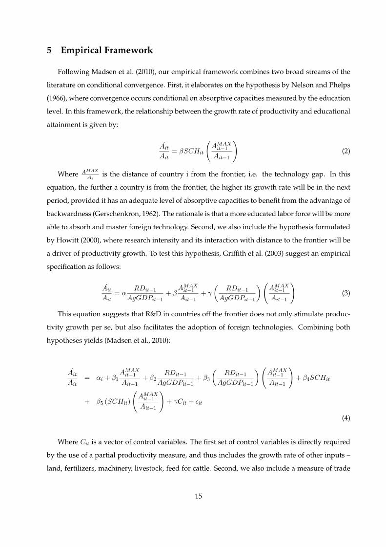
5 Empirical Framework

Following Madsen et al. (2010), our empirical framework combines two broad streams of the

literature on conditional convergence. First, it elaborates on the hypothesis by Nelson and Phelps

(1966), where convergence occurs conditional on absorptive capacities measured by the education

level. In this framework, the relationship between the growth rate of productivity and educational

attainment is given by:

Ait

Ait= βSCHit

(AMAX

it−1Ait−1

)(2)

Where AMAX

Aiis the distance of country i from the frontier, i.e. the technology gap. In this

equation, the further a country is from the frontier, the higher its growth rate will be in the next

period, provided it has an adequate level of absorptive capacities to benefit from the advantage of

backwardness (Gerschenkron, 1962). The rationale is that a more educated labor force will be more

able to absorb and master foreign technology. Second, we also include the hypothesis formulated

by Howitt (2000), where research intensity and its interaction with distance to the frontier will be

a driver of productivity growth. To test this hypothesis, Griffith et al. (2003) suggest an empirical

specification as follows:

Ait

Ait= α

RDit−1AgGDPit−1

+ βAMAX

it−1Ait−1

+ γ

(RDit−1

AgGDPit−1

)(AMAX

it−1Ait−1

)(3)

This equation suggests that R&D in countries off the frontier does not only stimulate produc-

tivity growth per se, but also facilitates the adoption of foreign technologies. Combining both

hypotheses yields (Madsen et al., 2010):

Ait

Ait= αi + β1

AMAXit−1Ait−1

+ β2RDit−1

AgGDPit−1+ β3

(RDit−1

AgGDPit−1

)(AMAX

it−1Ait−1

)+ β4SCHit

+ β5 (SCHit)

(AMAX

it−1Ait−1

)+ γCit + εit

(4)

Where Cit is a vector of control variables. The first set of control variables is directly required

by the use of a partial productivity measure, and thus includes the growth rate of other inputs –

land, fertilizers, machinery, livestock, feed for cattle. Second, we also include a measure of trade

15

openness. In addition to being potentially correlated with institutional characteristics favoring en-

trepreneurship, and to foster the equalization of prices by reducing the friction with international

markets, this variable also captures the potential to acquire knowledge embedded in imported

goods (Madsen et al., 2009).

6 Regression Results

This section presents the results of the fixed effects estimation of the conditional convergence

equation (4) in Section 5, with Table 3 showing estimates for all countries and then three different

subsamples: OECD countries, middle-income countries (both upper and lower) and less devel-

oped countries (LDCs). The difference with the results in Table 1 are clear. The estimated coeffi-

cients on distance to the frontier (DTF) are statistically significant and positive for both the entire

sample as well as the UMI/LMI subsample of developing countries. This finding, in line with

the results of Griffith et al. (2003), Kneller (2005), Kneller and Stevens (2006), and Madsen (2007,

2008) for the manufacturing sector, suggests that conditional on both the level of research intensity

and educational attainment, when productivity increases at the frontier in one period, off-frontier

countries will grow faster in the next period. In other words, labor productivity growth seems to

occur as a result of autonomous transfer of foreign technology in developing countries, irrespec-

tive of investments in R&D and the education level. This effect is not observed though for the

LDCs, taken as a subsample, suggesting that there may be further barriers or impediments to the

use of foreign technology. At the same time the sample size is also considerably reduced for this

group (19 countries with an average of 6 out of the 10 five-year time periods).

16

Tabl

e3:

Pane

lReg

ress

ions

ofLa

bor

Prod

ucti

vity

Gro

wth

(1a)

(1b)

(2a)

(2b)

(3a)

(3b)

(4a)

(4b)

All

coun

trie

s(8

3)O

ECD

(21)

UM

I/LM

I(44

)LD

Cs

(19)

lnD

TFit−1

0.03

79**

*0.

0358

***

0.01

740.

0419

0.05

43**

*0.

0594

***

0.02

170.

0251

(0.0

00)

(0.0

00)

(0.1

93)

(0.1

17)

(0.0

00)

(0.0

00)

(0.2

94)

(0.1

70)

R&

Dit−1

0.61

8***

0.56

3***

0.45

2**

0.43

8*1.

578*

*1.

487*

*-4

.247

-3.8

59(0

.000

)(0

.000

)(0

.021

)(0

.051

)(0

.012

)(0

.030

)(0

.110

)(0

.102

)(l

nD

TFx

R&

D) it−

1-0

.180

***

-0.1

83**

*-0

.101

-0.1

26-0

.444

***

-0.4

59**

0.82

50.

755

(0.0

00)

(0.0

00)

(0.3

66)

(0.3

86)

(0.0

06)

(0.0

14)

(0.1

46)

(0.1

33)

lnSc

h it

0.00

649

0.03

660.

0137

**-0

.011

7*(0

.137

)(0

.148

)(0

.029

)(0

.065

)ln

DTF

it−1

xln

Sch i

t-0

.000

0074

8-0

.000

272

-0.0

0008

810.

0001

90(0

.921

)(0

.455

)(0

.370

)(0

.117

)TO

g it

0.00

786

0.00

714

0.03

69**

*0.

0321

***

0.00

871

0.00

505

0.00

257

0.00

253

(0.1

02)

(0.1

26)

(0.0

00)

(0.0

02)

(0.1

22)

(0.3

33)

(0.8

22)

(0.8

12)

Land

g it

0.21

6***

0.21

5***

0.10

000.

148

0.12

3*0.

130*

0.26

7***

0.28

2***

(0.0

00)

(0.0

00)

(0.5

43)

(0.3

30)

(0.0

82)

(0.0

62)

(0.0

05)

(0.0

03)

Fert

g it

0.00

309

0.00

519

0.03

100.

0375

-0.0

0593

0.00

0614

0.00

506

0.00

433

(0.5

87)

(0.3

69)

(0.6

11)

(0.5

49)

(0.7

03)

(0.9

71)

(0.3

73)

(0.4

51)

Mac

hgit

0.01

730.

0386

**0.

138

0.17

20.

0285

0.05

30**

0.03

220.

0153

(0.3

05)

(0.0

15)

(0.5

37)

(0.4

76)

(0.3

37)

(0.0

24)

(0.2

63)

(0.6

08)

Live

g it

0.09

44**

0.10

2**

-0.0

411

0.00

0261

0.14

9***

0.16

1***

0.06

850.

0529

(0.0

29)

(0.0

20)

(0.7

46)

(0.9

98)

(0.0

07)

(0.0

06)

(0.4

61)

(0.5

69)

Feed

g it

0.04

70**

0.04

99**

0.01

930.

0050

90.

0166

0.02

680.

0938

***

0.09

55**

*(0

.031

)(0

.024

)(0

.826

)(0

.956

)(0

.568

)(0

.386

)(0

.003

)(0

.001

)

Obs

erva

tion

s45

445

411

011

024

424

497

97C

ount

ries

8383

1919

4444

1919

R2

0.54

0.55

0.51

0.54

0.49

0.52

0.62

0.64

Not

es:F

ixed

effe

cts

regr

essi

ons.

Coe

ffici

ents

are

repo

rted

wit

hp-

valu

esin

brac

kets

,wit

hro

bust

stan

dard

erro

rs.*

,**,

***

indi

cate

ssi

gnifi

canc

eat

the

10%

,5%

,and

1%le

vels

.

17

The coefficient on agricultural research intensity (R&D) is positive and statistically significant

for the whole sample and also for subsamples, with the exception of the LDCs. This suggests that

R&D does have an impact on the growth rate of productivity, which is consistent with most of

the empirical evidence found in the literature (see for example Pardey et al., 2013). The partial

effect of R&D appears much stronger for middle-income countries than for OECD countries but

it is necessary to take account of the interaction term with DTF as well, which provides a direct

estimate of the impact of research intensity at different levels of technological development. In

contrast with the macroeconomic literature on conditional convergence suggesting an advantage

from "backwardness" (Gerschenkron, 1962), investments in R&D seem to have a lower impact the

further a country is from the technological frontier, all else equal. In other words, R&D invest-

ments are more effective for more productive countries. Using the coefficient in specification (1a),

we can calculate the partial effect of research intensity, and the break-even point in terms of DTF

at which R&D starts to lose its impact on the growth rate of productivity. Given our coefficients,

the impact of research intensity disappears when the distance to the frontier is greater than about

22, (25 when using only the UMI/LMI subsample).9 These results suggest a more nuanced picture

of the productivity impacts of R&D than usually found in the literature.

Various explanations can be suggested for the decreasing effectiveness of R&D as one is further

from the frontier. One is that there might be some threshold level of R&D intensity necessary to see

substantial effectiveness. Looking at Figure 4, it is clear that since the 1980s, the research intensity

of OECD countries has been considerably higher than any of the developing countries, where this

intensity has actually even declined in recent decades (for LMI countries and LDCs). This suggests

an additional explanation related to the growth in private agricultural R&D in OECD countries,

which accounts for most of the overall growth. The dataset does not capture private R&D for

other groups of countries though this certainly much lower. It may therefore be the case that this

private R&D has driven most of the advancement of the frontier, while public R&D has possibly

been less effective. Although there is plenty of micro evidence of the returns to public agricultural

research in some OECD economies, especially in the U.S. (as noted above), this evidence is less

widespread for developing countries. Furthermore, concerns have been raised in the past about

the effectiveness of public agricultural research and extension services in developing countries,

from both efficiency and priority-setting perspectives (Kiers et al., 2008). Thus our results, in

failing to find an overall positive effect from R&D across income groups, may reflect these various

effects.9The DTF in our sample averages approximately 6 for OECD countries, 21 for UMI, 50 for LMI and 108 for LDCs

18

One additional factor to consider is the introduction of modern biotechnology and, in particu-

lar, genetically modified (GM) crops, in a number of OECD countries in the 1990s. A considerable

portion of the increase in R&D expenses in the U.S. and some other countries, especially by the

private sector have led to the development of a range of GM crop varieties, with consequent in-

creases in agricultural productivity. Regulatory regimes have differed though between countries

and meant that this new technology has not diffused to the large majority of countries in the sam-

ple. This could be interpreted as also accounting for a seemingly perverse result on the impact of

R&D. In particular, it makes it more difficult for countries to benefit from backwardness if they are

constrained by regulations from using one of the predominant technologies moving the frontier

forward. It is not possible to identify the extent of such an effect and it is important to recall that

we are here looking at aggregate agricultural productivity. It is also worth recalling that some

middle income countries in the sample, such as China, Argentina, and Brazil, have adopted a

number of GM crops with consequent productivity benefits.

To address the potentially long gestation period inherent to the R&D process (Alston, 2010;

Pardey et al., 2014), we also include 2 period-lags for R&D, suggesting that benefits are expected

to occur within a 5-10 year time span. Although anecdotal evidence from the biotech technology

suggest the time lag between the commercial release of a new technology and adoption occurs

within 10-13 years, and accounting for the 10-20 years necessary for the production of knowledge

to turn research input into output and regulatory approval could require a 20-30 years time lag.

To test this, we also include estimates of 2 and 3 lags, 3 and 4 lags, and 4 and 5 lags (20-25 years)

with results in the Appendix. However, the statistical significance of the impact or R&D on labor

productivity growth disappears when considering more than 2-period lags. This could be due

to the fact that most countries off the technology frontier invest in adaptive R&D, requiring a

shorter knowledge production period. Also, regulatory issues might not be as important in many

countries. But these additional lags also considerably reduce the number of observations in our

sample, implying that the results should be interpreted with caution.

The coefficient for the education variable also suggests nuanced conclusions. The level of

education in the country is often cited as a precondition for mastering technology (Evenson and

Fuglie, 2010). More educated farmers may be more efficient managers and also more likely to

adopt newer technologies. Our results suggest that increasing the proportion of the population

with some amount of secondary schooling has a positive impact on productivity growth for upper

middle income and lower middle income countries. While one might not expect to see an impact

in OECD countries, it is noteworthy that the coefficient for education for the sub-sample of 19 least

19

developed countries is negative (and significant at a 10 percent level). This might reflect a type

of urban bias among such countries, assuming that the increases in access to secondary education

might have benefitted primarily urban populations and that this is correlated with general policy

bias against agriculture and rural areas (Kydd and Dorward, 2001).

Trade openness is included as a control as in Madsen et al. (2010). Greater trade openness can

be expected to facilitate the inflow of foreign technologies, particularly through imports. In the

agricultural sector, one can think of imports of various inputs such as farm machinery, agrochem-

icals, or plant seeds and animal genetic stock. Trade openness might also be a proxy for licensing

and technology imported through increased foreign direct investment. The results indicate that

overall trade openness is not related to agricultural productivity. It does appear to play a positive

role though among the OECD countries, which have the highest level of productivity growth. In

and of itself though, it does not appear to play a strong role among developing countries. It is im-

portant to note though that this is an aggregate measure of trade openness and it may not apply as

much to agricultural goods for which tariff reduction has been much less than for manufactured

goods.

Among the other inputs, the coefficient on land is significant and positive in developing coun-

tries, though not in OECD. It is important to recall that this variable accounts for differences be-

tween irrigated and non-irrigated land. Thus the results likely reflect the increase in irrigation

among both middle income and least developed countries over this period.

7 Explaining Productivity Growth in Developing Countries

The results above of the conditional convergence analysis point to a number of unanswered

questions concerning why productivity-enhancing technology fails to generally flow from ad-

vanced economies to developing countries. This section explores further potential causes for ob-

served variation in the growth rates of productivity for developing countries. We now dispense

with the Madsen et al. (2010) specification of technological diffusion, based on distance to the

frontier, and sequentially incorporate various regressors in a simple fixed effects model to explain

labor productivity growth. This approach builds on the work of Headey et al. (2010), and Evenson

and Fuglie (2010), by using the updated Fuglie dataset and by controlling for unobserved hetere-

ogeneity. The sequential progression of specifications is partly determined by data availability,

which becomes quite limited for certain variables of interest.

We are primarily interested in institutional and policy factors that have been identified in the

20

literature as important determinants of agricultural productivity growth through improvements

in the efficiency of production using current technologies or the development and diffusion of

new technologies. These include R&D, education, trade openness, intellectual property rights,

infrastructure, support to the agricultural sector, growth in non-agricultural sectors, and the inci-

dence of conflict. Results are presented for middle income countries and LDCs in Tables 4 and 5

respectively.

The education level of farmers is expected to influence their capacity or inclination to master

new agricultural techniques (Evenson and Fuglie, 2010) and the mechanism is similar to its inclu-

sion in the original Nelson-Phelps model. Data on education levels among farmers or even rural

areas is limited. We therefore resort to using standard population-wide measures of education,

specifically the proportion of the population that has some amount of secondary education (Barro

and Lee, 2013). There is more variation in secondary education than in primary education, as the

latter has become more widely available.10

Education appears to be more important for less developed countries than for lower and upper

middle income countries (UMI/LMI). For the latter group, the coefficient on education is not sig-

nificant for specifications including multiple explanatory variables. On the other hand, for LDCs,

education remains significantly positive through all specifications, suggesting that it influences

agricultural productivity particularly when both existing productivity and availability of educa-

tion is lower. For less developed countries, the elasticity of productivity growth with respect to

the proportion of the population benefitting from secondary education is approximately 0.5-0.6.

Although the specification we use is different from Evenson and Fuglie (2010), our results are

consistent.11

Trade openness (TO) still does not appear to play much of a role in productivity growth. Some

specifications yield significant results for the coefficient on this variable but this is not generally

robust to different configurations of explanatory variables. For example, for UMI/LMI countries

this, statistical significance on the coefficient of trade openness disappears when we also control

for R&D, non-agricultural growth or for the rate of assistance to agriculture and a similar result

is seen in LDCs. This suggests that trade openness itself is not necessarily an important factor

for agricultural productivity growth but that in other specifications, it may be correlated with and

capturing the effects of general non-agricultural sector growth, discussed below.

10Evenson and Fuglie (2010) use the average years of schooling from Barro and Lee (2013). We found more significantresults by using the proportion of the population with secondary schooling.

11The approach of Evenson and Fuglie does not though immediately distinguish between the effects of educationfrom those of extension services as these are combined in a ‘Technology Mastery’ index.

21

Next, we reconsider the role of R&D together with intellectual property rights (IPRs) as a re-

lated institutional factor. The role of IPRs in stimulating or hindering technological change and

diffusion has been the subject of considerable debate and some analysis (see for overviews Moser,

2013; Eaton and Graff, 2014; Evenson and Swanson, 2010). IPRs such as patents, plant variety

rights, trademarks and trade secret protection, may stimulate innovation, by internalizing knowl-

edge externalities, and may also stimulate technology transfer through imports, licensing and for-

eign direct investment. On the other hand IPRs might inhibit international technological diffusion

where imitation is relatively easy, if their introduction and enforcement increases prices in coun-

tries where previously such technologies could be copied at little cost. Their importance in this

regard, relative to other factors affecting innovation and diffusion of new technologies, appears

mixed, varies by sectors and is clearly an empirical issue. In our analysis, we use lagged values

of the Ginarte and Park index to reduce the chance of endogeneity and also to allow for improve-

ments in this institutional variable to take effect. Any effects from policies or regulatory changes

to extend IPRs or improve their enforceability cannot be expected to work instantaneously. Given

the expected relationship between R&D and IPRs, we also include an interaction term.12

We find that R&D seems to have no effect on agricultural productivity growth in middle-

income countries. At first this seems inconsistent with the findings from the convergence speci-

fications. However the partial effect of R&D in the earlier analysis also needs to take account of

the interaction term with the distance to frontier, which will yield estimates that are negative. In

Table 5 the coefficient estimate on R&D for LDCs is significantly negative across all specifications

in which it is included. The partial effect for R&D is not though statistically different from zero

given the size and standard errors of the coefficient on the interaction between R&D and IPRs.

The results appear to indicate that IPRs have a somewhat positive effect on labor productivity

growth for UMI/LMI countries but a negative effect in less developed countries. The first of these

two findings would seem plausible and in line with the conclusions of others that IPRs are not

likely to have much effect at low levels of economic development where other factors constitute

more important constraints on innovation or adoption of existing technologies. Once a country

has reached a certain level of economic development, then some of these other constraints, such

as general education and technological capability among firms, may have been eased and IPRs

can, for example, facilitate access to newer technologies. Similarly as the level of technological

sophistication increases, technologies closer to the frontier, which are more likely to be protected

12The results with the interaction term are reported for LDCs only (see Table 5) as they were considerably different.In the case of middle income countries, the inclusion of the interaction term did not alter the results substantially andso these are not included in Table 4 in the interest of brevity.

22

by IPRs in other countries, may become more relevant or appropriate.

The significance of the coefficient on IPRs for middle income countries is however not robust

across all specifications, and varies considerably in size, suggesting misspecification issues. The

Ginarte and Park index, composed of five sub-indices, includes only a few dimensions that may be

directly relevant for the agricultural sector. These include plant variety rights. It may be argued

that general patent protection promotes the licensing and importing of a range of technologies

in chemicals and machineries that can be relevant for agriculture. It is possible though that this

IPR variable is correlated with and capturing the effects of other aspects that are favorable to

technological diffusion and that are not captured in our regressions. One might be the overall

regulatory environment and ease of investment and doing business. In particular, the Ginarte and

Park index is likely to be correlated with the quality of the contracting environment.

The negative coefficient on IPRs for LDCs might at first suggest that the implementation of

such regimes actually serves to restrict the unlicensed or unauthorized flow of foreign technolo-

gies into those countries. However once the interaction with R&D is taken into account, the total

partial effect of IPRs is not statistically different from zero. Although the specification is clearly not

satisfactory, we posit that the evidence is not pointing towards an important role for IPRs in pro-

moting innovation and technology diffusion in LDCs, nor in middle income countries. It would

be interesting to include other explanatory variables for aspects of the business and contracting

environment that may be confounding the specific effects of IPRs. We were though unable to find

such variables available for sufficient periods and leave this to future work.

Given the substantial number of observations with negative growth rates, especially in LDCs,

it seems relevant to control for the incidence of civil or international conflict and its negative ef-

fects on agricultural production, as was done by Headey et al. (2010).13 Whereas their analysis

was essentially cross-sectional, our panel data approach estimates the effects of the onset of con-

flict on agricultural productivity. Furthermore we recognize the long-term effects that conflict is

reputed to have on agricultural productivity by lagging this variable (C), which also helps reduce

potential endogeneity concerns. We screen out low intensity conflicts and select only conflicts

which caused more than 1,000 deaths cumulatively. Somewhat surprisingly the results are not as

strong as might be expected. The significance of the conflict variable is not robust across specifi-

cations for UMI/LMI countries. For LDCs, its negative effect is significant (in the most complete

specification), although the sample then consists of only 18 countries.

We also examine the effects of including nonagricultural productivity growth through two ad-

13See also Fulgitini and Perrin (1998).

23

ditional explanatory variables, the proportion of the rural population engaged in non-agricultural

activities (Non-Ag Pop) and the growth in non-agricultural GDP (Non-Ag GDP). This has not

generally been included in previous studies on agricultural productivity growth on which we

build, but does have a longer tradition in the development economics literature, going back at

least as far as the work of Lewis (1954), and the concept of surplus, underemployed labor in

agriculture. Recently Gollin et al. (2014) have noted and examined how labor productivity is

systematically higher in the nonagricultural sector than in agriculture, even after accounting for

potential measurement errors in effective labor and in value added. Related literature has looked

at the greater amount of cross-country variation in physical productivity in agriculture than in the

nonagricultural sector (Caselli, 2005; Restuccia et al., 2008; Chanda and Dalgaard, 2008). Proposed

explanations of this misallocation of labor across sectors include distortions that reduce farm size,

low intermediate usage in agriculture (Restuccia et al., 2008), selection of lower-ability workers

into agriculture (Lagakos and Waugh, 2013), and institutional frictions to labor mobility out of

agriculture (Gollin et al., 2014).

Under any of these scenarios, one would expect nonetheless that growth in the nonagricultural

economy would induce some labor reallocation and consequent productivity effects. Growth, and

increases in labor productivity, in other sectors can increase their relative return to labor and wage

rates, thus drawing labor out of agriculture and stimulating increases in productivity of labor

use in agriculture. There may also be a demand-side effect operating through output markets,

as nonagricultural growth increases the demand for final agricultural products.There is not suffi-

cient data to distinguish between these two different effects. We see that nonagricultural growth

has a significantly positive effect on agricultural productivity growth in middle income countries

but not in LDCs. We interpret these results with caution however, as there is potentially also an

element of reverse causality, with agricultural productivity growth releasing labor for use in other

sectors. This push vs pull relationship between agricultural and nonagricultural sector growth

has been the subject of considerable analysis and discussion in agricultural development litera-

ture (Gardner, 2005; Dorward, 2013). To try to reduce the potential for reverse causality, we also

used lagged nonagricultural growth (results non shown), but this generally did not lead to signifi-

cant coefficients. The relative importance of nonagricultural employment in rural areas also yields

a significant coefficient estimate, though for reduced sample size. Thus even the development of

the rural non-farm sector may play a role in driving agricultural labor productivity.

For UMI/LMI countries we also assess the importance of two other factors related to policy: in-

frastructure and agricultural support policy. Rural infrastructure, in particular roads, are expected

24

to be important for supporting agricultural growth, by reducing transport costs and supporting

market integration. The coefficient for the density of the road network (ROAD) is however not

significant. It may be though that UMI/LMI countries already have achieved reasonable levels of

infrastructural development, at least in terms of roads. The importance of roads may be stronger

in LDCs. Unfortunately there is insufficient data available to assess this.

Protectionist agricultural policy is reflected by the real rate of assistance to agriculture (RRA)

in terms of protection from world prices for farm output. Conventional theory posits that this sup-

port distorts relative prices and stimulates less efficient use of resources. The results presented do

not find any evidence that an increase in such support affects agricultural productivity, though in

some specifications we tried the coefficient was statistically significant and positive. The inclusion

of RRA however reduces the sample size to only 24 countries. All the same the role of shielding

producers from world markets may deserve further analysis. One conjecture could be that such

measures are serving in part to reduce output price volatility facing farmers.

25

26

Tabl

e4:

Expl

aini

ngLa

bor

Prod

ucti

vity

Gro

wth

(1a)

(1b)

(1c)

(1d)

(1e)

(1f)

(1g)

(1h)

(1i)

UM

I/LM

I

lnSc

h it−

10.

0068

5***

0.00

760*

**0.

0020

00.

0046

70.

0046

70.

0065

20.

0070

80.

0052

80.

0082

8(0

.002

)(0

.001

)(0

.415

)(0

.302

)(0

.303

)(0

.101

)(0

.102

)(0

.488

)(0

.110

)TO

g it

0.01

17**

0.01

29**

0.00

844

0.00

875

0.01

05*

0.00

122

0.01

06*

0.00

604

(0.0

46)

(0.0

24)

(0.1

38)

(0.1

27)

(0.0

88)

(0.8

51)

(0.0

85)

(0.3

41)

IPRit−1

0.00

900*

**0.

0049

9**

0.00

500*

*0.

0026

10.

0022

50.

0089

9*0.

0030

5(0

.000

)(0

.022

)(0

.021

)(0

.243

)(0

.335

)(0

.052

)(0

.171

)R

&D

it−1

-0.1

52-0

.150

-0.0

687

-0.1

07-0

.003

77-0

.155

(0.2

51)

(0.2

57)

(0.7

64)

(0.4

56)

(0.9

82)

(0.6

34)

Cit−1

-0.0

0279

-0.0

0538

-0.0

0247

-0.0

0319

-0.0

0517

(0.5

00)

(0.2

66)

(0.5

09)

(0.5

03)

(0.3

48)

Non

-Ag

Pop i

t0.

0520

***

(0.0

07)

Non

-Ag

GD

P it

0.13

4**

(0.0

21)

RO

AD

it−1

-0.0

0293

(0.6

15)

RR

Ait−1

0.00

721

(0.5

94)

Land

g it

0.16

2***

0.16

7***

0.17

6***

0.10

10.

0989

0.06

530.

110*

0.13

7*0.

0854

(0.0

06)

(0.0

04)

(0.0

10)

(0.1

13)

(0.1

26)

(0.4

29)

(0.0

79)

(0.0

98)

(0.2

68)

Fert

g it

0.03

73**

0.02

270.

0117

0.00

159

0.00

143

0.00

753

-0.0

0611

-0.0

187

0.00

706

(0.0

23)

(0.1

13)

(0.4

53)

(0.9

26)

(0.9

33)

(0.6

65)

(0.7

11)

(0.4

03)

(0.6

94)

Mac

hgit

0.04

76**

0.04

94**

0.04

70**

*0.

0574

**0.

0571

**0.

0533

*0.

0607

**0.

0445

0.04

11(0

.020

)(0

.016

)(0

.006

)(0

.023

)(0

.026

)(0

.056

)(0

.015

)(0

.178

)(0

.141

)Li

veg i

t0.

283*

**0.

242*

**0.

200*

**0.

185*

**0.

188*

**0.

212*

**0.

173*

**0.

195*

**0.

194*

**(0

.000

)(0

.000

)(0

.000

)(0

.000

)(0

.000

)(0

.001

)(0

.001

)(0

.001

)(0

.002

)Fe

edg i

t0.

0519

**0.

0427

**0.

0480

**0.

0462

0.04

680.

0364

0.04

400.

0658

*0.

0315

(0.0

42)

(0.0

45)

(0.0

15)

(0.1

49)

(0.1

46)

(0.3

45)

(0.1

58)

(0.0

91)

(0.4

66)

Obs

erva

tion

s52

546

740

524

624

614

524

019

113

9C

ount

ries

6161

5045

4524

4438

24R

20.

230.

260.

270.

320.

310.

410.

340.

330.

37

Not

es:F

ixed

effe

cts

regr

essi

ons.

Coe

ffici

ents

are

repo

rted

wit

hp-

valu

esin

brac

kets

,wit

hro

bust

stan

dard

erro

rs.*

,**,

***

indi

cate

ssi

gnifi

canc

eat

the

10%

,5%

,and

1%le

vels

.

Table 5: Explaining Labor Productivity Growth

(1a) (1b) (1c) (1d) (1e)

LDCs

ln Schit−1 0.00597*** 0.00605*** 0.00808* 0.00859** 0.00964**(0.003) (0.005) (0.057) (0.030) (0.014)

TOgit 0.0116** 0.0128 0.0149 0.0109(0.045) (0.260) (0.163) (0.384)

IPRit−1 -0.0120* -0.0118* -0.0158**(0.060) (0.072) (0.049)

R&Dit−1 -1.125*** -1.111** -1.125**(0.009) (0.013) (0.024)

(IPR x R&D)it−1 0.545** 0.534** 0.589**(0.014) (0.020) (0.020)

Cit−1 -0.00937 -0.0180**(0.332) (0.018)

Non-Ag GDPit 0.166(0.107)

Landgit 0.219** 0.236*** 0.276* 0.270* 0.294**(0.012) (0.009) (0.053) (0.064) (0.030)

Fertgit 0.0161** 0.00826** 0.00316 0.00206 0.00637(0.023) (0.047) (0.627) (0.768) (0.350)

Machgit 0.0264 0.00937 0.0218 0.0158 -0.00737(0.232) (0.687) (0.514) (0.682) (0.842)

Livegit 0.201*** 0.144*** 0.117 0.122 0.109(0.000) (0.006) (0.244) (0.246) (0.287)

Feedgit 0.0978*** 0.0871*** 0.0944** 0.0973** 0.0753*(0.008) (0.002) (0.018) (0.018) (0.063)

Observations 246 210 98 98 89Countries 28 28 20 20 18R2 0.42 0.42 0.36 0.36 0.38

Notes: Fixed effects regressions. Coefficients are reported with p-values in brackets,with robust standard errors. *,**, *** indicates significance at the 10%, 5%, and 1% levels.

8 Summary and Conclusion

This paper has explored international productivity patterns in agriculture, re-examining evi-

dence for convergence across countries. The results highlight the differentiated impact of R&D

and education at different levels of technological development. We find that R&D has a statisti-

cally significant impact on labor productivity growth, but that this impact is lower the further a

country is from the technological frontier, in contrast with predictions from the macroeconomic

literature on productivity convergence. The productivity-enhancing effect of research intensity is

therefore less clear for LDCs.

Our results on convergence, both unconditional and conditional, contrast with some earlier

27

findings, most notably those of Martin and Mitra (2001). Three salient differences may account

for this: two based on the dataset and the third on our specification. One is the longer dataset,

although if anything, there is more evidence towards converging growth rates in the additional

1995-2010 period included in the Fuglie (2012) dataset (see Figure 3). The second difference is

the adjustments made for the quality of inputs in the productivity estimates by Fuglie. These

seem to affect developing countries more than OECD countries, and most of the sample period is

characterized by clear gaps in productivity growth rates between groups of countries according

to overall income levels.

The third difference is our conditional convergence specification, which draws on recent macroe-

conomic literature and controls for the influence of R&D, as well as its interaction with the distance

to the frontier. Given the limited and imperfect data, we are reticent to draw unequivocal policy

recommendations from our analysis. We do though see the as potentially uncovering interesting

aspects deserving further investigation. For example, our results do support previous analysis

that has questioned the effectiveness of agricultural R&D in developing countries, highlighting

institutional biases and constraints (Kiers et al., 2008). Our results do not necessarily imply that

such investments should be assigned lower priority. If anything, our findings highlight the im-

portance of considering both quantity and quality of investments in national agricultural research

systems. Much of the current literature concentrates on the arguments for increasing the quan-

tity, such as those by Alston and Pardey (2014); Pardey et al. (2010, 2013), with good reason given

observed declines in agricultural R&D over the longer term in many countries.

We also estimated a relatively straightforward regression of labour productivity growth on a

range of explanatory variables in an attempt to update the results of Headey et al. (2010). One

difference is that we now control for unobserved heterogeneity as well as using the Fuglie pro-

ductivity dataset. These results are generally far from satisfactory. Nonetheless they do point to

a strong role for education in promoting productivity growth in LDCS, though not necessarily

in middle income countries. Trade openness also appears to have had an effect on productivity

in middle income countries. IPRs do not seem on the other hand to be as relevant and further

analysis could find ways to disentangle the effects from the influence of other aspects of the legal

environment that can influence business and investment opportunities. More interestingly, ours

is the first paper to consider the possible role of growth in the nonagricultural sector. We sug-

gest that this may also warrant further analysis, given the role such growth might have played in

driving agricultural productivity growth in middle income countries.

28

Appendix A Sample

Table A1: Country Sample

Country Inc. group Country Inc. group Country Inc. group

Australia OECD Bulgaria UMI Pakistan LMIAustria OECD Chile UMI Papua New Guinea LMICanada OECD Colombia UMI Paraguay LMIDenmark OECD Costa Rica UMI Philippines LMIEstonia OECD Cuba UMI Sri Lanka LMIFinland OECD Dominican Republic UMI Sudan LMIFrance OECD Fiji UMI Swaziland LMIGermany OECD Gabon UMI Syrian Arab Republic LMIGreece OECD Hungary UMI Tajikistan LMIIceland OECD Iran, Islamic Rep. UMI Thailand LMIIreland OECD Jamaica UMI Tunisia LMIItaly OECD Jordan UMI Ukraine LMIJapan OECD Kazakhstan UMI Yemen, Rep. LMIKorea, Rep. OECD Libya UMI Zambia LMINetherlands OECD Malaysia UMI Afghanistan LDCNew Zealand OECD Mauritius UMI Armenia LDCNorway OECD Mexico UMI Bangladesh LDCPoland OECD Namibia UMI Benin LDCPortugal OECD Panama UMI Burundi LDCSpain OECD Peru UMI Cambodia LDCSweden OECD Romania UMI Central African Republic LDCSwitzerland OECD South Africa UMI Congo, Rep. LDCUnited Kingdom OECD Turkey UMI Gambia, The LDCUnited States OECD Uruguay UMI Ghana LDCBahrain High Inc. Venezuela, RB UMI Guyana LDCBrunei Darussalam High Inc. Bolivia LMI Haiti LDCCyprus High Inc. Cameroon LMI Kenya LDCIsrael High Inc. China LMI Lao PDR LDCKuwait High Inc. Cote d’Ivoire LMI Liberia LDCLatvia High Inc. Ecuador LMI Malawi LDCLithuania High Inc. Egypt, Arab Rep. LMI Mali LDCMalta High Inc. El Salvador LMI Mozambique LDCQatar High Inc. Guatemala LMI Myanmar LDCRussian Federation High Inc. Honduras LMI Nepal LDCSaudi Arabia High Inc. India LMI Niger LDCTrinidad and Tobago High Inc. Indonesia LMI Rwanda LDCUnited Arab Emirates High Inc. Iraq LMI Senegal LDCAlbania UMI Kyrgyz Republic LMI Sierra Leone LDCAlgeria UMI Lesotho LMI Tanzania LDCArgentina UMI Mauritania LMI Togo LDCBelize UMI Mongolia LMI Uganda LDCBotswana UMI Morocco LMI Vietnam LDCBrazil UMI Nicaragua LMI Zimbabwe LDC

29

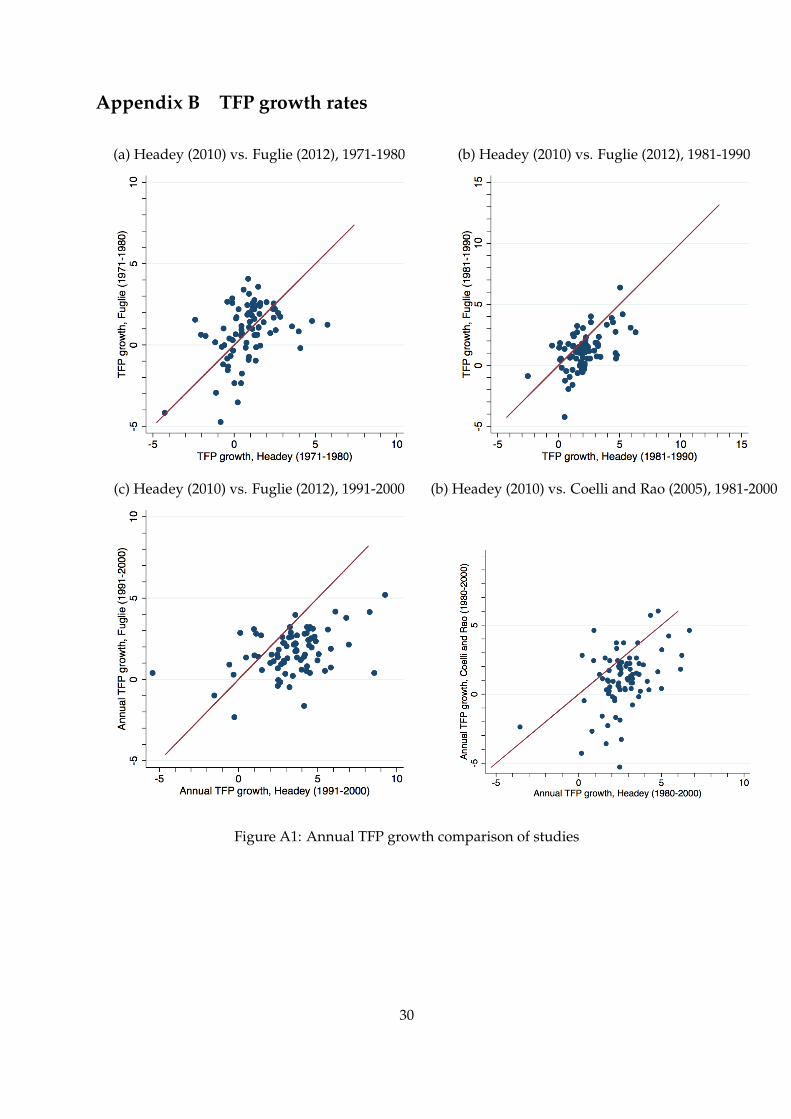
Appendix B TFP growth rates

(a) Headey (2010) vs. Fuglie (2012), 1971-1980 (b) Headey (2010) vs. Fuglie (2012), 1981-1990

(c) Headey (2010) vs. Fuglie (2012), 1991-2000 (b) Headey (2010) vs. Coelli and Rao (2005), 1981-2000

Figure A1: Annual TFP growth comparison of studies

30

Appendix C Additional lags for R&D

Table A2: Additional Lags

(1a) (1b) (1c) (1d)

Whole sample

ln DTFit−1 0.0546*** 0.0686*** 0.0734*** 0.0766***(0.000) (0.001) (0.001) (0.000)

R&Dit−1 0.364*(0.052)

ln DTFit−1 x R&Dit−1 -0.124**(0.012)

R&Dit−2 0.357** 0.573***(0.034) (0.001)

ln DTFit−1 x R&Dit−2 -0.0834 -0.114(0.315) (0.119)

R&Dit−3 -0.110 0.00944(0.506) (0.954)

ln DTFit−1 x R&Dit−3 0.00654 -0.0327(0.894) (0.673)

R&Dit−4 -0.0223 -0.0813(0.844) (0.532)

ln DTFit−1 x R&Dit−4 0.000259 -0.0160(0.996) (0.779)

R&Dit−5 0.112(0.454)

ln DTFit−1 x R&Dit−5 0.0108(0.898)

ln Schit 0.0167 0.0295** 0.0382** -0.00610(0.111) (0.028) (0.047) (0.760)

ln DTFit−1 x ln Schit -0.000747 -0.00173 -0.00213 -0.000754(0.392) (0.138) (0.177) (0.598)

Landgit 0.221*** 0.152** 0.0761 0.0977(0.000) (0.024) (0.337) (0.350)

Fertgit 0.000140 0.00566 0.00579 0.00574(0.984) (0.464) (0.528) (0.478)

Machgit 0.0594*** 0.0361 0.0248 0.0583*(0.006) (0.112) (0.533) (0.090)

Livegit 0.0929* 0.0882 0.0806 0.110**(0.087) (0.243) (0.294) (0.047)

Feedgit 0.0572** 0.0354* 0.0346 0.0150(0.014) (0.068) (0.126) (0.575)

N 352 299 253 206Countries 76 73 66 63R2 0.51 0.51 0.46 0.57

Notes: p-values in parentheses. * p < 0.05, ** p < 0.01, *** p < 0.001

31

References

Abramovitz, M. (1990) “The Catch–up Factor in Postwar Economic Growth,” Economic Inquiry,

Vol. 28:1, pp. 1–18.

Acemoglu, D. and F. Zilibotti (2001) “Productivity Differences,” The Quarterly Journal of Economics,

Vol. 116:2, pp. 563–606.

Alene, A.D. (2010) “Productivity growth and the effects of R&D in African agriculture,” Agricul-

tural Economics, Vol. 41, pp. 223–238.

Alston, J. M. (2010) “The Benefits from Agricultural Research and Development, Innovation, and

Productivity Growth,” Food, Agriculture and Fisheries Working Paper No. 31, Organisation for

Economic Cooperation and Development, Paris, France.

Alston, J. M. and P.G. Pardey (2014) “Agriculture in the Global Economy,” Journal of Economic

Perspectives,, Vol. 28(1), pp. 121–46.

Alston, J.M., M.C. Marra, P.G. Pardey, and T.J. Wyatt (2000) “A meta analysis of rates of return

to agricultural R&D: Ex pede Herculem?” International Food Policy Research Institute, Vol. IFPRI

Research Report no 113.

Anderson, K. and E. Valenzuela (2008) “Estimates of Global Distortions to Agricultural Incentives,

1955 to 2007„” World Bank, Washington DC, Vol. available at www.worldbank.org/agdistortions.

Barro, R. and J.W. Lee (2013) “A new data set of educational attainment in the world, 1950-2010,”

Journal of Development Economics, Vol. 104, pp. 184–198.

Barro, R. and X. Sala-i Martin (1997) “Technological Diffusion, Convergence and Growth,” Journal

of Economic Growth, Vol. 2, pp. 1–27.

Beintema, N.M. and G.J. Stads (2006) “Agricultural R&D in Sub–Saharan Africa: an Era of Stag-

nation, Background Report,” International Food Policy Research Institute.

Benhabib, J. and M. Spiegel (1994) “The role of human capital in economic development evidence

from aggregate cross-country data,” Journal of Monetary Economics, Vol. 34.

Bernard, A.B. and C.I. Jones (1996) “Productivity Across Industries and Countries: Time Series

Theory and Evidence,” The Review of Economics and Statistics, Vol. 78, pp. 135–146.

32

Calderon, C. and L. Serven (2004) “The effects of infrastructure development on growth and in-

come distribution,” World Bank Policy Research Working Paper, Vol. 3400.

Capalbo, S.M. and J.M. Antle (1988) “Agricultural productivity: measurement and explanation,”

Resources for the Future, Washington D.C.

Caselli, F. (2005) “Accounting for Cross-Country Income Differences„” in P. Aghion and S. Durlauf

eds. Handbook of Economic Growth, pp. 679–741.

Chanda, A. and C.-J. Dalgaard (2008) “Dual Economies and International Total Factor Productivity

Differences: Channelling the Impact from Institutions, Trade, and Geography,” Economica, Vol.

75, pp. 629–661.

Coelli, T.J. and D. P. Rao (2005) “Total factor productivity growth in agriculture: a Malmquist

index analysis of 93 countries, 1980–2000,” Agricultural Economics, Vol. 32, pp. 115–134.

Craig, B. J., P.G. Pardey, and J. Roseboom (1997) “International Productivity Patterns,: Accounting

for Input Quality, Infrastructure and Research,” American Journal of Agricultural Economics, Vol.

79, pp. 1064–1076.

Dorward, Andrew (2013) “Agricultural labour productivity, food prices and sustainable develop-

ment impacts and indicators,” Food Policy, Vol. 39, pp. 40–50.

Dowrick, S. and D.-T. Nguyen (1989) “OECD Comparative Economic Growth 1950–85: Catch–Up

and Convergence,” The American Economic Review, Vol. 79, pp. 1010–1030.

Eaton, D. and G. Graff (2014) “The dynamic IP system in crop genetics and biotechnology,” in

Stuart Smyth, Peter W. B Phillips, and David Castle eds. Handbook on Agriculture, Biotechnology

and Development, Cheltenham, UK: Edward Elgar.

Eberhardt, M. and F. Teal (2012) “No Mangoes in the Tundra: Spatial Heterogeneity in Agricultural

Productivity Analysis,” Oxford Bulletin of Economics and Statistics.

Evenson, R.E. and K.E. Fuglie (2010) “Technology capital: the price of admission to the growth

club,” Journal of Productivity Analysis, Vol. 33, pp. 173–190.

Evenson, R.E. and T. Swanson (2010) “Technological Change and Technological Diffusion in

Agricultural Development: How have Proprietary Rights Contributed?” in Keith E. Maskus,

Joseph E. Stiglitz, and Jerome H Reichman eds. The Economics of Intellectual Property Rights and

Innovation, Knowledge, and Technology Transfer, Princeton N.J.: Princeton University Press.

33

Fare, R., S. Grosskopf, M. Norris, and Z. Zhang (1994) “Productivity Growth, Technical Progress,

and Efficiency Change in Industrialized Countries,” The American Economic Review, Vol. 84:1,

pp. 66–83.

Fuglie, K., S.L. Wang, and V.E. Ball (2012) Productivity Growth in Agriculture: An International Per-

spective: CAB International Wallingford.

Fuglie, K.O. (2012) “Productivity Growth and Technology Capital in the Global Agricultural Econ-

omy,” In: Productivity Growith in Agriculture: An International Perspective, pp. 335–368.

Fulgitini, L.E. and R. Perrin (1998) “Agricultural productivity in developing countries,” Agricul-

tural Economics, Vol. 19, pp. 45–51.

Gardner, Bruce L (2005) “Causes of rural economic development,” Agricultural Economics, Vol. 32,

pp. 21–41.

Gerschenkron, A. (1962) “Economic Backwardness in Historical Perspective,” Belknap Press of Har-

vard University Press.

Ginarte, J.C. and W.G. Park (1997) “Determinants of patent rights: A cross–national study,” Re-

search Policy, Vol. 26, pp. 283–301.

Gleditsch, N.P., P. Wallensteen, M. Eriksson, M. Sollenberg, and H. Strand (2002) “Armed Conflict

1946–2001: A New Dataset,” Journal of Peace Research, Vol. 39, pp. 615–637.

Gollin, D., D. Lagakos, and M.E. Waugh (2014) “The Agricultural Productivity Gap,” The Quarterly

Journal of Economics, Vol. 129, pp. 939–993.

Griffith, R., S. Redding, and J. Van Reenen (2003) “R&D and Absorptive Capacity: Theory and

Empirical Evidence,” Scandinavian Journal of Economics, Vol. 105, pp. 99–118.

Griliches, Z. (1964) “Research expenditures, education and the aggregate agricultural production

function,” The American Economic Review, Vol. 54, pp. 961–974.

Headey, D., M. Alauddin, and D.S. P. Rao (2010) “Explaining agricultural productivity growth: an

international perspective,” Agricultural Economics, Vol. 41, pp. 1–14.

Howitt, P. (2000) “Endogenous growth and cross-country income differences,” American Economic

Review, Vol. 90, pp. 829–46.

34

Islam, M.D.R., J.B. Ang, and J.B. Madsen (2014) “Quality-Adjusted Human Capital and Produc-

tivity Growth,” Economic Inquiry, Vol. 52, pp. 757–777.

James, J.S., P.G. Pardey, and J.M. Alston (2008) “Agricultural R&D Policy: A Tragedy of the Inter-

national Commons,” Instepp Paper 08-01.

Kiers, E. T., R. R. B. Leakey, A.-M. Izac, J. A. Heinemann, E. Rosenthal, D. Nathan, and J. Jiggins

(2008) “Agriculture at a Crossroads,” Science, Vol. 320, pp. 320–321.

Kneller, R. (2005) “Frontier technology, absorptive capacity and distance,” Oxford Bulletin of Eco-

nomics and Statistics, Vol. 67, pp. 1–23.

Kneller, R. and P.A. Stevens (2006) “Frontier Technology and Absorptive Capacity: Evidence from

OECD Manufacturing Industries,” Oxford Bulletin of Economics and Statistics, Vol. 68, pp. 1–21.

Kydd, Jonathan and Andrew Dorward (2001) “The Washington consensus on poor country agri-

culture: Analysis, prescription and institutional gaps,” Development Policy Review, Vol. 19, pp.

467–478.

Lagakos, D. and M. E. Waugh (2013) “Selection, Agriculture and Cross-Country Productivity Dif-

ferences,” American Economic Review, Vol. 103, pp. 948–980.

Lewis, W. A. (1954) “Economic Development With Unlimited Supply of Labor,” Manchester School

of Economic and Social Studies, Vol. 22, pp. 139–191.

Ludena, C., T. Hertel, P. Preckel, K. Foster, and A. Nin (2007) “Productivity growth and conver-

gence in crop, ruminant, and non-ruminant production: measurement and forecasts,” Agricul-

tural Economics, Vol. 37, pp. 1–17.

Madsen, J. (2007) “Technology spillover through trade and TFP convergence: 135 years of evi-

dence for the OECD countries,” Journal of International Economics, Vol. 72:2, pp. 464–480.

(2008) “Semi-endogenous versus Schumpeterian growth models: testing the knowledge

production function using international data,” Journal of Economic Growth, Vol. 13:1, pp. 1–26.

Madsen, J. B. and I. Timol (2011) “Long–Run Convergence in Manufacturing and Innovation–

Based Models,” The Review of Economics and Statistics, Vol. 93, pp. 1155–1171.

Madsen, J.B., M.D.R. Islam, and J.B. Ang (2010) “Catching up to the technology frontier: the di-

chotomy between innovation and imitation,” Canadian Journal of Economics, Vol. 43, pp. 1389 –

1411.

35

Madsen, J.B., S. Saxena, and J.B. Ang (2009) “The Indian growth miracle and endogenous growth,”

Journal of Development Economics.

Martin, W. and D. Mitra (2001) “Productivity Growth and Convergence in Agriculture versus

Manufacturing,” Economic Development and Cultural Change, Vol. 49, pp. 403–422.

Moser, P. (2013) “Patents and innovation: Evidence from economic history,” Journal of Economic

Perspectives, Vol. 27, pp. 23–44.

Nelson, R.R. and E.S. Phelps (1966) “Investment in humans, technological diffusion, and economic

growth,” American Economic Review, Vol. 56, pp. 69–75.

Pardey, P. and N. Beintema (2001) “Slow Magic: Agricultural R&D a Century After Mendel,”

IFPRI Working Paper.

Pardey, P., N. Beintema, S. Dehmer, and S. Wood (2006) “Agricultural Research: A Growing Global

Divide?” IFPRI Working Paper.

Pardey, P. G., C. Chan-Kang, S. Dehmer, J. M. Beddow, T. M. Hurley, X. Rao, and J. M. Alston

(2014) “Investments in and the Economic Returns to Agricultural and Food R&D Worldwide,”

in Neal K. Van Alfen ed. Encyclopedia of Agriculture and Food Systems, Oxford: Academic Press,

pp. 78–97.

Pardey, P. and J. Roseboom (1989) ISNAR Agricultural Research Indicator Series: A Global Data Base

on National Agricultural Research Systems: Cambridge University Press.

Pardey, P.G., J.M. Alston, and C. Chang-Kang (2013) “Public agricultural R&D over the past half

century: an emerging new world order,” Agricultural Economics, Vol. 44, pp. 103 – 113.

Pardey, P.G., J.M. Alston, and V.W. Ruttan (2010) “The Economics of Innovation and Technical

Change in Agriculture,” In: Handbooks in Economics, Vol. 2.

Pardey, P.G., J. Roseboom, and B.J. Craig (1997) “Agricultural R&D investments and impact,”

Paying for Agricultural Productivity, IFPRI, Vol. Chapter 3 in J.M. Alston, P.G. Pardey, and V.H.

Smith.

Pingali, P. L. and P.W. Heisey (1999) “Cereal Crop Productivity in Developing Countries: Past

Trends and Future Prospects,” Economics Working Papers, Vol. 99-03.

36

Rao, D. P. and T. Coelli (2004) “Catch–up and Convergence in Global Agricultural Productivity,”

Indian Economic Review, Vol. 39, pp. 123–148.

Restuccia, D., D. Tao Yang, , and X. Zhu (2008) “Agriculture and aggregate productivity: A quan-

titative cross-country analysis,” Journal of Monetary Economics, Vol. 55, pp. 234–250.

Rezitis, A.N. (2010) “Agricultural productivity and convergence: Europe and the United States,”

Applied Economics, Vol. 42, pp. 1029–1044.

Schimmelpfennig, D. and C. Thirtle (1999) “The Internationalization of Agricultural Technology:

Patents, R&D Spillovers, and Their Effects on Productivity in the European Union and United

States,” Contemporary Economic Policy, Vol. 17, pp. 457–468.

Suhariyanto, K. and C. Thirtle (2001) “Productivity growth and convergence in Asian agriculture,”

Journal of Agricultural Economics, Vol. 52, pp. 96–110.

Wang, S.L., P.W. Heisey, W.E. Huffman, and K.O. Fuglie (2013) “Public R&D, Private R&D, and

U.S. Agricultural Productivity Growth: Dynamic and Long-Run Relationships,” American Jour-

nal of Agricultural Economics, Vol. 95:5, pp. 1287–1293.

37