Research on static and dynamic heat balance of the … on static and dynamic heat balance of the ......

Research on static and dynamic heat balance of the human body

Dr. dr. h.c. LÁSZLÓ BÁNHIDI Professor Emeritus, Department of Building Service Engineering and Process Engineering, Budapest

University of Technology and Economics H-1111. Budapest, Műegyetem rkp. 3. Tel: +36 (1) 463 2405, e-mail: [email protected]

Dr. LÁSZLÓ GARBAI

Professor, Department of Building Service Engineering and Process Engineering, Budapest University of Technology and Economics

H-1111. Budapest, Műegyetem rkp. 3. Tel: +36 (1) 463 2405, e-mail: [email protected]

IMRICH BARTAL Ph.D. student, Department of Building Service Engineering and Process Engineering, Budapest University of

Technology and Economics H-1111. Budapest, Műegyetem rkp. 3. Tel: +36 (1) 463 2405, e-mail: [email protected]

Abstract: This paper attempts to give a brief summary of the concept, objectives and research methodology of comfort theory and, in particular, thermal comfort for international building service engineers. It also provides an overview of the findings of international research and the goals of ongoing Hungarian projects (mainly carried out at the Department of Building Service Engineering and Process Engineering at the Budapest University of Technology and Economics). Moreover, the importance of comfort theory and its application by engineers will be highlighted. We intend to present the basic equations of the classical comfort theory, the equations of the human body’s static heat balance, and the so called comfort equation as well as its sensitivity depending on the thermic parameters of the microclimate. The PMV expression describing the thermal comfort of the human body and its sensitivity, derivatives and cross-derivatives is emphasized, too. The concept of dynamic thermal sensation and the possibilities of its research is going to be introduced, which is possible only through the presentation of system theory, system dynamics and regulation theory. Keywords: Thermal Comfort, Static and Dynamic Heat Balance, Thermal Sensation, Human Body. 1 INTRODUCTION The architectural and building engineering design of spaces suitable for human occupation and work aims to meet the so-called comfort requirements optimally. Human comfort requirements cover the air quality of the occupied space and its thermal attributes in addition to other ergonomic, sociological and psychological criteria, they we naming parameters of microclimate. According to the research approach used in the last two decades (comfort theory, thermal comfort – research) the analysis of the joint impact of microclimate parameters can be based on the energy balance of an active or sedentary human who has a mechanical or thermal connection with his/her environment. 2 CLASSIFYING AND MEASURING THERMAL COMFORT Human response to thermal environment and the satisfaction with thermal comfort are expressed by

subjective thermal sensation. Thermal comfort is linked to the heat balance of the human body: the time and the adaptation reactions required to achieve this balance and whether it is agreeable for the given person and what skin temperature and perspiration are measured. ASHRAE expresses subjective thermal sensation using the thermal sensation scale: +3 (hot), +2 (warm), +1 (slightly warm), 0 (neutral), -1 (slightly cool), -2 (cool), -3 (cold) The agreeable thermal sensation falls between –1 and +1 on the scale. In an experiment conducted with several thousand live subjects the test persons had to declare (after a relaxation interval) how they felt in the examined microclimate and what value they voted for on the scale. P. O. Fanger based the investigation of thermal sensation on writing up and calculating the energy balance of the human body and established a mathematical connection between the solutions of the energy balance and the thermal sensation scale. [1]

WSEAS TRANSACTIONS on HEAT and MASS TRANSFER LÁSZLÓ BÁNHIDI,LÁSZLÓ GARBAI,IMRICH BARTAL

ISSN: 1790-5044 187 Issue 3, Volume 3, July 2008

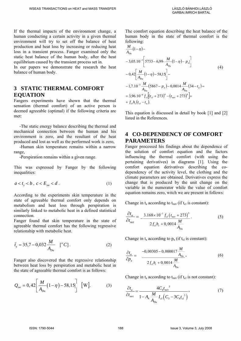
If the thermal impacts of the environment change, a human conducting a certain activity in a given thermal environment will try to set off the balance of heat production and heat loss by increasing or reducing heat loss in a transient process. Fanger examined only the static heat balance of the human body, after the heat equilibrium caused by the transient process set in. In our papers we demonstrate the research the heat balance of human body. 3 STATIC THERMAL COMFORT EQUATION Fangers experiments have shown that the thermal sensation (thermal comfort) of an active person is deemed agreeable (optimal) if the following criteria are met: -The static energy balance describing the thermal and mechanical connection between the human and his environment is zero, and the resultant of the heat produced and lost as well as the performed work is zero, -Human skin temperature remains within a narrow range, -Perspiration remains within a given range. This was expressed by Fanger by the following inequalities:

bta s << , dEc sw << . (1) According to the experiments skin temperature in the state of agreeable thermal comfort only depends on metabolism and heat loss through perspiration is similarly linked to metabolic heat in a defined statistical connection. Fanger found that skin temperature in the state of agreeable thermal comfort has the following regressive relationship with metabolic heat.

Dus A

Mt 032,07,35 −= ][ Co . (2)

Fanger also discovered that the regressive relationship between heat loss by perspiration and metabolic heat in the state of agreeable thermal comfort is as follows:

( )0, 42 1 58,15swDu

MQA

η⎡ ⎤

= − −⎢ ⎥⎣ ⎦

[ ]W . (3)

The comfort equation describing the heat balance of the human body in the state of thermal comfort is the following:

( )

( )

( )

( ) ( )

( ) ( )[ ]( ).

27327310.96,3

340014,0586710.7,1

15,58142,0

199,6573310.05,3

1

448

5

3

aclccl

mrtclcl

aDu

aDu

Du

aDu

Du

tthfttf

tAMp

AM

AM

pAM

AM

−+++−+=

=−−−−

−⎥⎦

⎤⎢⎣

⎡−−−

⎥⎦

⎤⎢⎣

⎡−−⋅−−

−−

−

−

−

η

η

η

(4)

This equation is discussed in detail by book [1] and [2] listed in the References. 4 CO-DEPENDENCY OF COMFORT PARAMETERS Fanger processed his findings about the dependence of the solution of comfort equation and the factors influencing the thermal comfort (with using the pertaining derivatives) in diagrams [1]. Using the comfort equation derivatives describing the co-dependency of the activity level, the clothing and the climate parameters are obtained. Derivatives express the change that is produced by the unit change on the variable in the numerator while the value of comfort equation remains zero, witch we are present in follows: Change in ta according to tmrt (if tcl is constant):

=∂∂

mrt

a

tt ( )373.168 10 273

2 0,0014

cl mrt

cl cDu

f tMf hA

−× +−

+

. (5)

Change in ta according to pa (if tcl is constant):

=∂∂

a

a

pt 0,00305 0,000017

2 0,0014

Du

cl cDu

MA

Mf hA

− −

+

. (6)

Change in ta according to tmrt (if tcl is not constant):

( )

34

34 5 4

4

1 3a mrt

mrtcl cl

Du

t C tMt A I C C tA

∂=

∂ − −. (7)



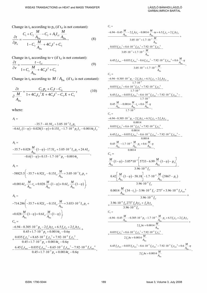
Change in ta according to pa (if tcl is not constant):

1 2 5 3

33 4 51 4

clDu Du

a

Du

M MC C C A IA At

Mp C C t CA

+ − +∂

=∂ − + +

. (8)

Change in ta according to v (if tcl is not constant):

33 4 51 4

cl

Du

t ttMv C C t CA

−∂=

∂ + + +. (9)

Change in ta according to / DuM A (if tcl is not constant):

2 3 03 3

4 4 5 51 4 4a

cl

Du

C p C t CtM C t X C t C X CA

+ −∂=

+ + − +∂, (10)

where:

( ) ( )

13

5

35.7 41.9 3.05 10 ,0.6 1 0.028 1 0.15 1.7 10 0.0014

cl cl a

cl cl a cl a cl

A

I I pI I p I t Iη η

−

−

=

− − + ⋅− − − − + − ⋅ −

( )

( )

2

3

5

35.7 0.028 1 17.5 3.05 10 24.4,

0.6 1 0.15 1.7 10 0.0014

cl cl a clDu

a a

AM I I p IA

p t

η

η

−

−

=

− + − − + ⋅ +

− − + − ⋅ −

( ) ( )

3

358823.5 35.7 6.92 0.15 3.05 10

0.0014 0.028 1 0.6 1 ,

cl cl cl aDu

cl a clDu Du Du

A

MI I I pA

M M MI t IA A A

η η

−

=

⎛− − + − + ⋅ +⎜

⎝⎞

+ + − + − ⎟⎠

( ) ( )

4

3714.286 35.7 6.92 0.15 3.033 10

0.028 1 0.6 1 ,

cl cl cl aDu

clDu Du

A

MI I I pA

M MIA A

η η

−

=

⎛− − + − + ⋅ +⎜

⎝⎞

+ − + − ⎟⎠

03

5

2 5 3 8 4

5

2 5

6.94 0.305 10 2 6.5 20.45 1.7 10 0.0014 0.6

0.035 8.65 10 7.92 100.45 1.7 10 0.0014 0.6

6.45 0.035 8.65 10

a cl c a cl cl cl c cl

a a

cl cl cl cl cl cl

a a

cl mrt cl mrt cl mrt

C

p f h t f t f h tp t

f t f t f tp t

f t f t f t

η

η

−

−

− −

−

−

=

− − ⋅ − + ++

+ ⋅ + −

+ ⋅ + ⋅+ −

+ ⋅ + −

− − ⋅−

3 8 4

5

7.92 10 ,0.45 1.7 10 0.0014 0.6

cl mrt

a a

f tp t η

−

−

− ⋅+ ⋅ + −

1

3 5

2 5 3 8 4

3 5

2 3 8

6.94 0.45 2 0.0014 6.5 2

3.05 10 1.7 10

0.035 8.6 10 7.92 10

3.05 10 1.7 10

6.45 0.035 8.6 7.92 10

cl c a cl cl cl c clDu Du

Du

cl cl cl cl cl cl

Du


CM Mf h t ta f t f h tA A

MA

f t f t f tMA

f t f t f t f

− −

− −

− −

−

=

− − − − + ++

⋅ + ⋅

+ ⋅ + ⋅+ −

⋅ + ⋅

− − − ⋅−

4

3 5

0.6,

3.05 10 1.7 10

cl mrtDu

Du

MtA

MA

η

− −

+

⋅ + ⋅

23

5

2 5 3 8 4

5

2 5 3 8 4

5

6.94 0.305 10 2 6.5 21.7 10

0.035 8.6 10 7.92 101.7 10

6.45 0.035 8.6 10 7.92 101.7 10

0.45 0.001


cl cl cl cl cl cl

cl mrt cl mrt cl mrt cl mrt

Du

C

p f h t f t f h t

f t f t f t

f t f t f t f t

MA

−

−

− −

−

− −

−

=

− − ⋅ − + ++

⋅+ ⋅ + ⋅

+ −⋅

− − ⋅ − ⋅ −− −

⋅

−− 5

4 0.6,

1.7 10

aDu Du

M MtA A

η

−

+

⋅

33

2 5 3 8 4

2 5 3 8 4

5

6.94 0.305 10 2 6.5 20.0014

0.035 8.6 10 7.92 100.0014

6.45 0.035 8.6 10 7.92 100.0014

0.45 1.7 10


cl cl cl cl cl cl

cl mrt cl mrt cl mrt cl mrt

Du D

C

p f h t f t f h t

f t f t f t

f t f t f t f t

M MA A

−

− −

− −

−

=

− − ⋅ − + ++

+ ⋅ + ⋅+ −

− − ⋅ − ⋅ −− −

− ⋅−

0.6,

0.0014

au Du

MpA

η+

( ) ( )

( ) ( )

( )

4

3

8

5

8

8 4 8 4

8

8 4

1 3.05*10 5733 6.99 1

3.96 10

0.42 1 58.18 1.7 10 5867

3.96 10

0.0014 34 3.96 10 273 3.96 10

3.96 10

3.96 10 273

aDu Du

cl

aDu Du

cl

a cl cl mrtDu

cl

cl cl

C

M M pA A

f

M M pA A

fM t f f tA

f

f f

η η

η

−

−

−

−

− −

−

−

=

⎡ ⎤− − − − −⎢ ⎥

⎣ ⎦ −⋅

⎡ ⎤− − − ⋅ −⎢ ⎥

⎣ ⎦− −⋅

− − ⋅ ⋅ + ⋅− +

⋅

⋅+ 8 ,

3.96 10c cl cl c a

cl

h t f h tf−

+⋅

5

3 5

2 5 3 8 4

2 5 3 8

6.94 0.45 0.305 10 1.7 10 6.5 2

2 0.0014

0.035 8.6 10 7.92 10

2 0.0014

6.45 0.035 8.6 10 7.92 10

a a cl cl cl c clDu Du

clDu

cl cl cl cl cl cl

clDu


CM Mp p f t f h tA A

Mf hcA

f t f t f tMf hcA

f t f t f t

− −

− −

− −

=

− − − ⋅ − ⋅ + ++

+

+ ⋅ + ⋅+ −

+

− − ⋅ − ⋅−

4 0.6,

2 0.0014

cl mrtDu

clDu

Mf tA

Mf hcA

η+

+



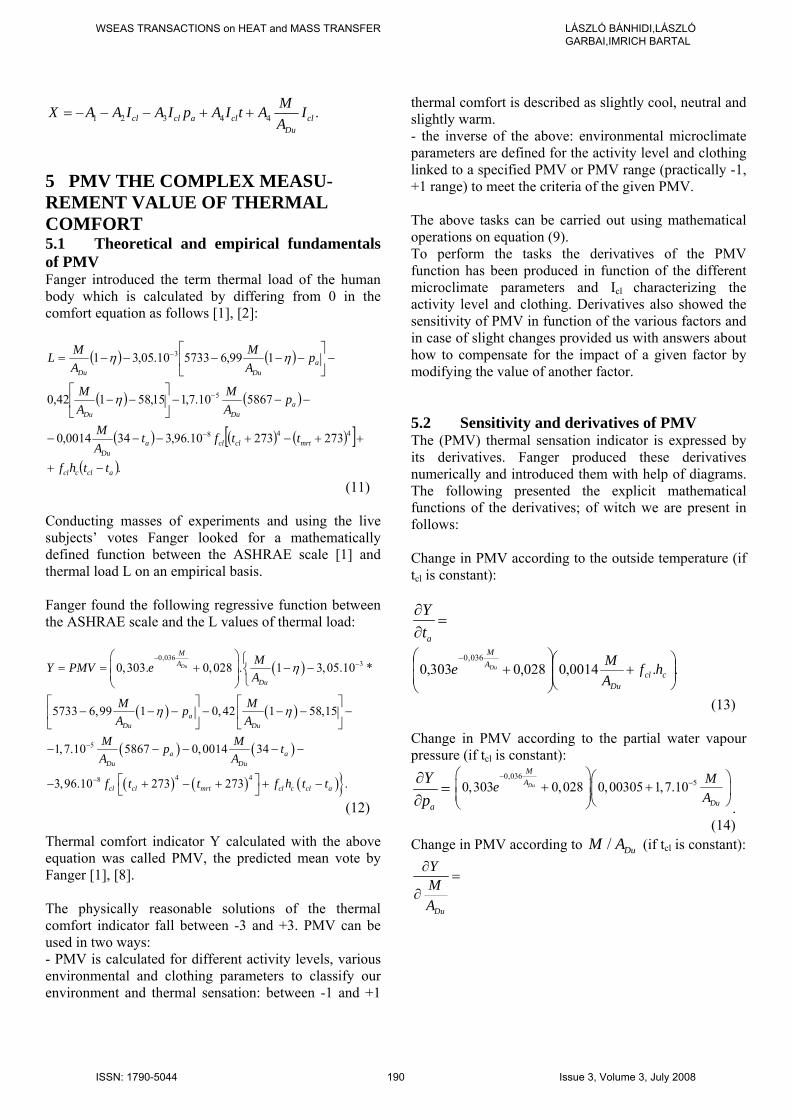
1 2 3 4 4 .cl cl a cl clDu

MX A A I A I p A I t A IA

= − − − + +

5 PMV THE COMPLEX MEASU- REMENT VALUE OF THERMAL COMFORT 5.1 Theoretical and empirical fundamentals of PMV Fanger introduced the term thermal load of the human body which is calculated by differing from 0 in the comfort equation as follows [1], [2]:

( ) ( )

( ) ( )

( ) ( ) ( )[ ]( ).

27327310.96,3340014,0

586710.7,115,58142,0

199,6573310.05,31

448

5

3

aclccl

mrtclclaDu

aDuDu

aDuDu

tthf

ttftAM

pAM

AM

pAM

AML

−+

++−+−−−

−−−⎥⎦

⎤⎢⎣

⎡−−

−⎥⎦

⎤⎢⎣

⎡−−−−−=

−

−

−

η

ηη

(11) Conducting masses of experiments and using the live subjects’ votes Fanger looked for a mathematically defined function between the ASHRAE scale [1] and thermal load L on an empirical basis. Fanger found the following regressive function between the ASHRAE scale and the L values of thermal load:

( )

( ) ( )

( ) ( )

( ) ( ) ( )}

0,0363

5

4 48

0,303. 0,028 . 1 3,05.10 *

5733 6,99 1 0, 42 1 58,15

1,7.10 5867 0,0014 34

3,96.10 273 273 .

Du

MA

Du

aDu Du

a aDu Du

cl cl mrt cl c cl a

MY PMV eA

M MpA A

M Mp tA A

f t t f h t t

η

η η

−−

−

−

⎛ ⎞ ⎧= = + − −⎜ ⎟ ⎨⎜ ⎟ ⎩⎝ ⎠

⎡ ⎤ ⎡ ⎤− − − − − − −⎢ ⎥ ⎢ ⎥

⎣ ⎦ ⎣ ⎦

− − − − −

⎡ ⎤− + − + + −⎣ ⎦

(12) Thermal comfort indicator Y calculated with the above equation was called PMV, the predicted mean vote by Fanger [1], [8]. The physically reasonable solutions of the thermal comfort indicator fall between -3 and +3. PMV can be used in two ways: - PMV is calculated for different activity levels, various environmental and clothing parameters to classify our environment and thermal sensation: between -1 and +1

thermal comfort is described as slightly cool, neutral and slightly warm. - the inverse of the above: environmental microclimate parameters are defined for the activity level and clothing linked to a specified PMV or PMV range (practically -1, +1 range) to meet the criteria of the given PMV. The above tasks can be carried out using mathematical operations on equation (9). To perform the tasks the derivatives of the PMV function has been produced in function of the different microclimate parameters and Icl characterizing the activity level and clothing. Derivatives also showed the sensitivity of PMV in function of the various factors and in case of slight changes provided us with answers about how to compensate for the impact of a given factor by modifying the value of another factor. 5.2 Sensitivity and derivatives of PMV The (PMV) thermal sensation indicator is expressed by its derivatives. Fanger produced these derivatives numerically and introduced them with help of diagrams. The following presented the explicit mathematical functions of the derivatives; of witch we are present in follows: Change in PMV according to the outside temperature (if tcl is constant):

a

Yt∂

=∂

..0014,0028,0303,0036,0

⎟⎟⎠

⎞⎜⎜⎝

⎛+

⎟⎟⎠

⎞⎜⎜⎝

⎛+

−

cclDu

AM

hfAMe Du

(13) Change in PMV according to the partial water vapour pressure (if tcl is constant):

a

Yp∂

=∂

0,03650,303 0,028 0,00305 1,7.10Du

MA

Du

MeA

−−

⎛ ⎞⎛ ⎞+ +⎜ ⎟⎜ ⎟⎜ ⎟⎝ ⎠⎝ ⎠ .

(14) Change in PMV according to / DuM A (if tcl is constant):

Du

YMA

∂=

∂



( )(

( ) ( ) )

( ) ( )

( ) ( ) ( )( )( )

( ) ( ) .115,58142,0

199,6573300305,0

273273109,3

340014,05867107,1

010908,0139865,0340014,0

5867107,11028,0303,0

448

5

036,0

5036,0

⎟⎟⎠

⎞−+⎟⎟

⎠

⎞⎜⎜⎝

⎛−−−

−⎟⎟⎠

⎞⎜⎜⎝

⎛−−−−

−+−+⋅−−−

⎜⎜⎝

⎛−−−−−⋅−

⋅−−−−−−

−−⋅−⋅⎟⎟

⎠

⎞

⎜⎜

⎝

⎛+

−

−

−

−

ηη

η

ηη

DuDu

Dua

mrtclclaclccl

aDu

aDu

AM

a

aAM

AM

AM

AMp

ttftthf

tAMp

AM

et

pe

Du

Du

(15) Change in PMV according to the mean radiant temperature (if tcl is constant):

mrt

Yt∂

=∂

( ) .273028,0303,010584,1 3036,0

7mrtcl

AM

tfe Du +⎟⎟

⎠

⎞

⎜⎜

⎝

⎛+⋅

−−

(16) Change in PMV according to hc (if tcl is constant):

c

Yh∂

=∂ ( )

0,0360,303 0,028 . .Du

MA

cl cl ae f t t−⎛ ⎞

− + −⎜ ⎟⎜ ⎟⎝ ⎠

(17) Change in PMV according to air velocity (if tcl is constant):

=∂∂

vY ( )

0,0366,05 0,303 0,028

.

Du

MA

cl c a

a

e f t t

v

−⎛ ⎞+ −⎜ ⎟⎜ ⎟

⎝ ⎠−

(18) Change in PMV according to hc (if tcl is not constant):

c

Yh∂

=∂

( ) ( )( )

( )

( )( )

0,036

37 2

37

37

0,303 0,028 *

1,584 10 273

1,584 10 273 1

.1,584 10 273 1

Du

MA

cl cl cl cl acl cl a

cl cl cl cl cl c

cl cl clcl c

cl cl cl cl cl c

e

f t I t tf t t

I f t I f h

I f t taf h

I f t I f h

−

−

−

−

⎛ ⎞+⎜ ⎟⎜ ⎟

⎝ ⎠⎛ ⎞⋅ ⋅ + −⎜ ⎟− + −⎜ ⎟− ⋅ + + +⎝ ⎠

⎛ ⎞−⎜ ⎟−⎜ ⎟− ⋅ + + +⎝ ⎠

(19) Change in PMV according to the ambient temperature (if tcl is not constant):

=∂∂

atY

( )( )

( )( )

0,036

37 2

37

37

0,303 0,028

1,584 10 273

1,584 10 273 1

.1,584 10 273 1

Du

MA

cl cl cl cl ccl c

cl cl cl cl cl c

cl cl clcl c

cl cl cl cl cl c

e

f t I t hf h

I f t I f h

I f t taf h

I f t I f h

−

−

−

−

⎛ ⎞+ ⋅⎜ ⎟⎜ ⎟

⎝ ⎠⎛ ⋅ ⋅ +⎜ − +⎜ − ⋅ + + +⎝

⎞⎛ ⎞−⎟⎜ ⎟−

⎜ ⎟⎟− ⋅ + + +⎝ ⎠⎠

(20) Change in PMV according to the mean radiant temperature (if tcl is not constant):

=∂∂

mrttY

( ) ( )( )

( )

( )( )

0,036

3 314 237

37

37

37

0,303 0,028 *

2,509056 10 273 2731,584 10 273

1,584 10 273 1

1,584 10 273

1,584 10 273 1

Du

mrt

MA

cl cl cl mrtcl

cl cl cl cl cl c

cl cl mrtcl c

cl cl cl cl cl c

e

f t I tf t

I f t I f h

I f tf h

I f t I f h

−

−−

−

−

−

⎛ ⎞+⎜ ⎟⎜ ⎟

⎝ ⎠⎛ ⋅ ⋅ + +⎜ − ⋅ +⎜ − ⋅ + + +⎝

⎛ ⋅ +

− ⋅ + + +.⎞⎞⎟⎜ ⎟

⎜ ⎟⎟⎝ ⎠⎠ (21) Change in PMV according to / DuM A (if tcl is not constant):

=∂

∂

DuAMY

( )

( ) ( )

( ) ( ) ( )( )( ) ( )

0,036

5

4 48

37

7

0,010908 0,603195 1 6,93735

0,00305 1,7 10 5867 0,014 34

3,96 10 273 273

1,584 10 273 0,028 0,028

1,584 10

Du

MA

Du

a a aDu Du

cl cl mrt cl c cl a

cl cl

cl cl cl

MeA

M Mp p tA A

f t t f h t t

f t

I f t

η

η

−

−

−

−

−

⎛ ⎞ ⎛− ⋅ − + +⎜ ⎟ ⎜⎜ ⎟ ⎝⎝ ⎠

+ − ⋅ − − − −

− ⋅ + − + − − −

⋅ + −−− ⋅ ( )

( )( )

3

8

37

273 1

3,96 10 0,028 ,028.

1,584 10 273 1

cl cl c

cl c

cl cl cl cl cl c

I f h

f h

I f t I f h

η−

−

++ + +

⎞⋅ −⎟+⎟− ⋅ + + + ⎠

(22) 6 DYNAMIC HEAT BALANCE OF HUMAN BODY Many people examined the dynamic heat balance in the past years some of them: B. W. Olesen, Muhsin Kilic, Omer Kaynakli, Mihaela Baritz, Luciana Cristea, Diana Cotoros and Ion Balcu.



Mihaela Baritz, Luciana Cristea, Diana Cotoros and Ion Balcu are presented the differential equation describe the dynamic heat balance of human body, can by calculated as fallows [12]:

( )2

2 m bl bl bl artbl cT T Tk q w c T T

r r trω ρ ρ

⎛ ⎞∂ ∂ ∂+ + + − =⎜ ⎟∂ ∂∂⎝ ⎠

(23) TSENS and DISC values can be calculated by the following equations [10]:

( )( ) ( )

( )⎪⎩

⎪⎨

⎧

−+

−−

−

=

hbbe

cbhbcbbe

cbb

TTTTTT

TTTSENS

,

,,,

,

685,07,4/7,4

4685,0

ηη

bhb

hbbcb

cbb

TTTTT

TT

<

≤≤

<

,

,,

,

(24)

( )( )

⎪⎪⎩

⎪⎪⎨

⎧

−−

−

−

=

difereqrswee

reqrswerswe

cbb

QQQ

QQTT

DISC

,,,max,

,,,

,

7,44685,0

.,

,

bcb

cbb

TTTT≤

<

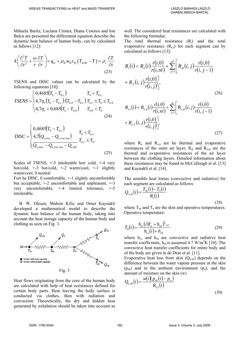
(25) Scales of TSENS, +-5 intolerable hot/ cold, +-4 very hot/cold, +-3 hot/cold, +-2 warm/cool, +-1 slightly warm/cool, 0 neutral Fort he DISC, 0 comfortable, +-1 slightly uncomfortable but acceptable, +-2 uncomfortable and unpleasant, +-3 very uncomfortable, +-4 limited tolerance, +-5 intolerable. B. W. Olesen, Muhsin Kilic and Omer Kaynakli developed a mathematical model to describe the dynamic heat balance of the human body, taking into account the heat storage capacity of the human body and clothing as seen on Fig. 3.

Fig. 3

Heat flows originating from the core of the human body are calculated with help of heat resistances defined for certain body parts. Heat leaving the body surface is conducted via clothes, then with radiation and convection. Theoretically, the dry and hidden heat generated by exhalation should be taken into account as

well. The considered heat resistances are calculated with the following formulas: The total thermal resistance (Rt) and the total evaporative resistance (Re,t) for each segment can by calculated as follows [13]:

( ) ( ) ( )( ) ( ) ( )

( )

( ) ( )( ) ,

,0,,

1,0,,

,0,

1

⎥⎦

⎤+

⎢⎣

⎡−

+= ∑=

jirirjiR

jirirjiR

nliririRiR

f

nl

jalat

(26)

( ) ( ) ( )( ) ( ) ( )

( )

( ) ( )( ) ,

,0,,

1,0,,

,0,

,

1,,,

⎥⎦

⎤+

⎢⎣

⎡−

+= ∑=

jirirjiR

jirirjiR

nliririRiR

fe

nl

jaleaete

(27) where Ra and Re,a are he thermal and evaporative resistances of the outer air layer, Ral and Re,al are the thermal and evaporative resistances of the air layer between the clothing layers. Detailed information about these resistances may be found in McCullough et al. [13] and Kaynakli et al. [14]. The sensible heat losses (convective and radiative) for each segment are calculated as follows:

( ) ( ) ( )( )iR

iTiTiQt

sksks

0,

−=

(28) where Tsk and To are the skin and operative temperatures. Operative temperature:

( ) ( )( ) rdcv

rdrdacv

hihThTihiT

++

=0 (29)

where hcv and hrd are convective and radiative heat transfer coefficients, hrd is assumed 4.7 W/m2K [10]. The convective heat transfer coefficients for entire body and of the body are given in de Dear et al. [11]. Evaporative heat loss from skin (Qe,sk) depends on the difference between the water vapour pressure at the skin (psk) and in the ambient environment (pa), and the amount of moisture on the skin (w)

( ) ( ) ( )( )( )iR

pipiwiQte

askske

,,

−=

(30)



Total skin wettedness (w) includes wettedness due to regulatory sweating (wrsw) and to diffusion through the skin (wdif). wrsw and wdif are given by:

max,e

fgrswrsw Q

hmw = (31)

( )rswdif ww −= 106,0 (32) where the Qe,max is the maximum evaporative potential, mrsw is the rate of sweat production, hfg the heat of vaporization of water. The blood flow between the core and skin per unit of skin area can be expressed mathematically as:

( )

36005,01

2003,6

1

⎥⎦

⎤⎢⎣

⎡++

= sk

cr

b

CSIGWSIG

m (33)

where WSIG and CSIG are warm and cold signal from the body thermoregulatory control mechanism, respectively. The heat exchange between the core and skin can be written as:

( )( )skcrblblpskcr TTmcKQ −+= ,, (34) where K is average thermal conductance, cp,bl is specific heat of blood. The rate of sweat production per unit of skin area is estimated by:

.7,10

exp107,4 5 ⎟⎠

⎞⎜⎝

⎛×= − skbrsw

WSIGWSIGm (35)

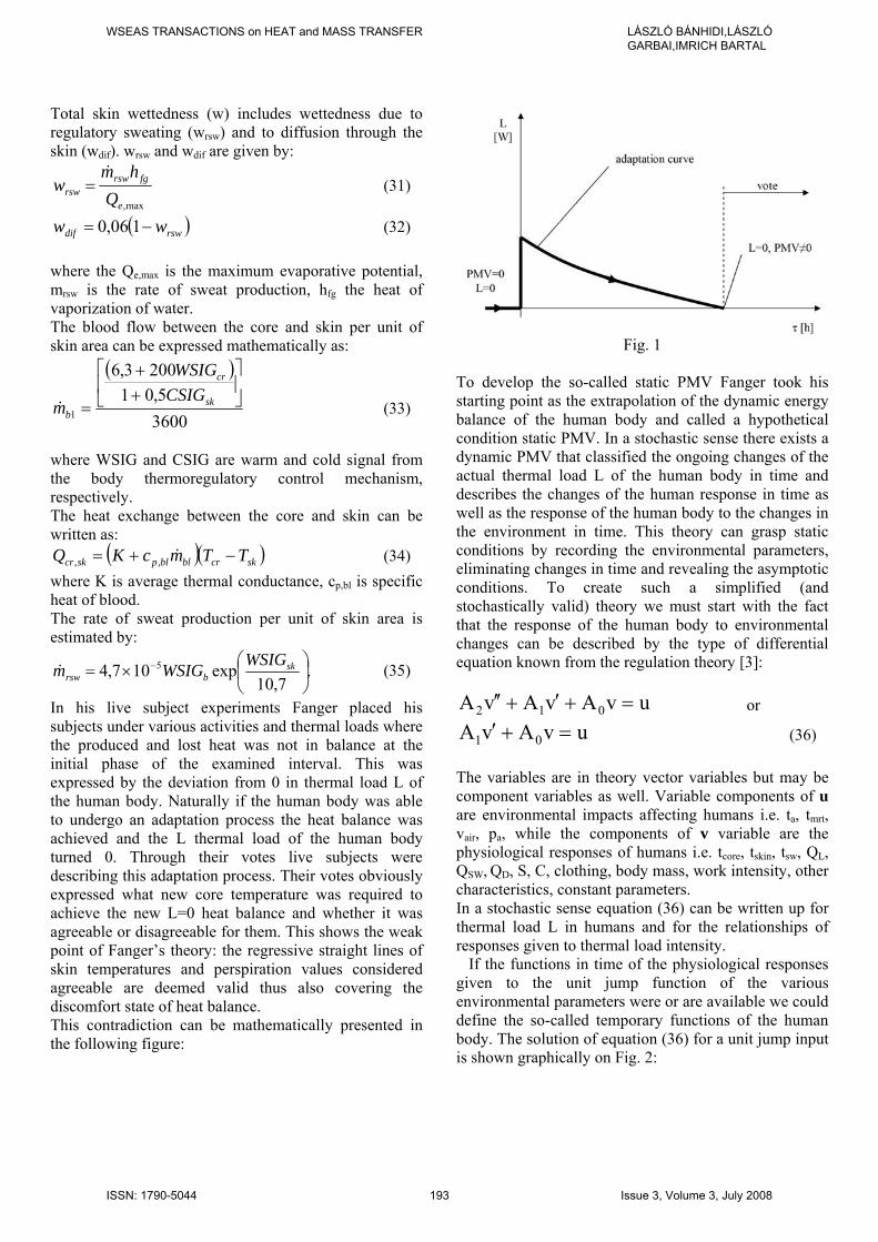
In his live subject experiments Fanger placed his subjects under various activities and thermal loads where the produced and lost heat was not in balance at the initial phase of the examined interval. This was expressed by the deviation from 0 in thermal load L of the human body. Naturally if the human body was able to undergo an adaptation process the heat balance was achieved and the L thermal load of the human body turned 0. Through their votes live subjects were describing this adaptation process. Their votes obviously expressed what new core temperature was required to achieve the new L=0 heat balance and whether it was agreeable or disagreeable for them. This shows the weak point of Fanger’s theory: the regressive straight lines of skin temperatures and perspiration values considered agreeable are deemed valid thus also covering the discomfort state of heat balance. This contradiction can be mathematically presented in the following figure:

Fig. 1

To develop the so-called static PMV Fanger took his starting point as the extrapolation of the dynamic energy balance of the human body and called a hypothetical condition static PMV. In a stochastic sense there exists a dynamic PMV that classified the ongoing changes of the actual thermal load L of the human body in time and describes the changes of the human response in time as well as the response of the human body to the changes in the environment in time. This theory can grasp static conditions by recording the environmental parameters, eliminating changes in time and revealing the asymptotic conditions. To create such a simplified (and stochastically valid) theory we must start with the fact that the response of the human body to environmental changes can be described by the type of differential equation known from the regulation theory [3]:

uvAvAvA 012 =+′+′′ or

uvAvA 01 =+′ (36) The variables are in theory vector variables but may be component variables as well. Variable components of u are environmental impacts affecting humans i.e. ta, tmrt, vair, pa, while the components of v variable are the physiological responses of humans i.e. tcore, tskin, tsw, QL, QSW, QD, S, C, clothing, body mass, work intensity, other characteristics, constant parameters. In a stochastic sense equation (36) can be written up for thermal load L in humans and for the relationships of responses given to thermal load intensity. If the functions in time of the physiological responses given to the unit jump function of the various environmental parameters were or are available we could define the so-called temporary functions of the human body. The solution of equation (36) for a unit jump input is shown graphically on Fig. 2:



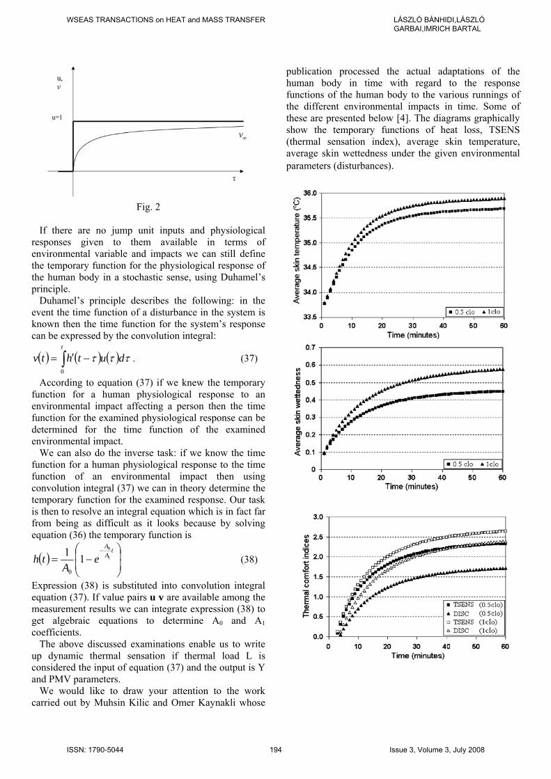
Fig. 2

If there are no jump unit inputs and physiological responses given to them available in terms of environmental variable and impacts we can still define the temporary function for the physiological response of the human body in a stochastic sense, using Duhamel’s principle. Duhamel’s principle describes the following: in the event the time function of a disturbance in the system is known then the time function for the system’s response can be expressed by the convolution integral:

( ) ( ) ( )∫ −′=t

duthtv0

τττ . (37)

According to equation (37) if we knew the temporary function for a human physiological response to an environmental impact affecting a person then the time function for the examined physiological response can be determined for the time function of the examined environmental impact. We can also do the inverse task: if we know the time function for a human physiological response to the time function of an environmental impact then using convolution integral (37) we can in theory determine the temporary function for the examined response. Our task is then to resolve an integral equation which is in fact far from being as difficult as it looks because by solving equation (36) the temporary function is

( ) ⎟⎟⎠

⎞⎜⎜⎝

⎛−=

− tAA

eA

th 1

0

11

0

(38)

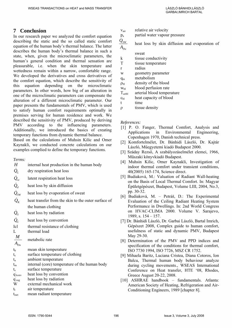
Expression (38) is substituted into convolution integral equation (37). If value pairs u v are available among the measurement results we can integrate expression (38) to get algebraic equations to determine A0 and A1 coefficients. The above discussed examinations enable us to write up dynamic thermal sensation if thermal load L is considered the input of equation (37) and the output is Y and PMV parameters. We would like to draw your attention to the work carried out by Muhsin Kilic and Omer Kaynakli whose

publication processed the actual adaptations of the human body in time with regard to the response functions of the human body to the various runnings of the different environmental impacts in time. Some of these are presented below [4]. The diagrams graphically show the temporary functions of heat loss, TSENS (thermal sensation index), average skin temperature, average skin wettedness under the given environmental parameters (disturbances).



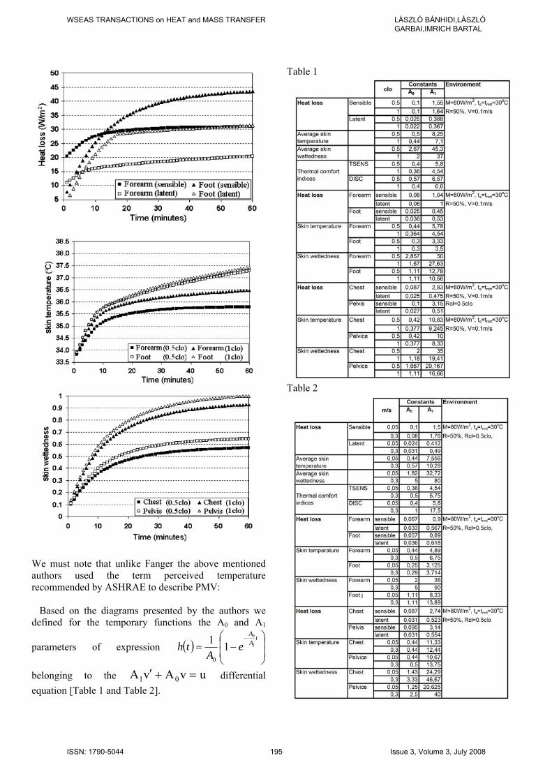
We must note that unlike Fanger the above mentioned authors used the term perceived temperature recommended by ASHRAE to describe PMV: Based on the diagrams presented by the authors we defined for the temporary functions the A0 and A1

parameters of expression ( ) ⎟⎟⎠

⎞⎜⎜⎝

⎛−=

− tAA

eA

th 1

0

11

0

belonging to the uvAvA 01 =+′ differential equation [Table 1 and Table 2].

Table 1

Table 2



7 Conclusion In our research paper we analyzed the comfort equation describing the static and the so called static comfort equation of the human body’s thermal balance. The latter describes the human body’s thermal balance in such a state, when, given the microclimatic parameters, the human’s general condition and thermal sensation are pleasurable, i.e. when the skin temperature and wettedness remain within a narrow, comfortable range. We developed the derivatives and cross derivatives of the comfort equation, which describe the sensitivity of this equation depending on the microclimatic parameters. In other words, how big of an alteration in one of the microclimatic parameters can compensate the alteration of a different microclimatic parameter. Our paper presents the fundamentals of PMV, which is used to satisfy human comfort requirements optimally in premises serving for human residence and work. We described the sensitivity of PMV, produced by deriving PMV according to the influencing parameters. Additionally, we introduced the basics of creating temporary functions from dynamic thermal balance. Based on the calculations of Muhsin Kilic and Omer Kaynakli, we conducted concrete calculations on our examples complied to define the temporary functions. Terms: H internal heat production in the human body

LQ dry respiration heat loss

reQ latent respiration heat loss

dQ heat loss by skin diffusion

SWQ heat loss by evaporation of sweat

KQ heat transfer from the skin to the outer surface of the human clothing

SQ heat loss by radiation

CQ heat loss by convention Icl thermal resistance of clothing L thermal load

Du

MA

metabolic rate

tb mean skin temperature tc surface temperature of clothing ta ambient temperature tm internal (core) temperature of the human body ts surface temperature q·

konv heat loss by convention q·

sug heat loss by radiation W external mechanical work tl air temperature tmrt mean radiant temperature

vair relative air velocity pa partial water vapour pressure

SW

Du

QA

heat loss by skin diffusion and evaporation of

sweat k tissue conductivity T tissue temperature r radius w geometry parameter qm metabolism ρbl density of the blood wbl blood perfusion rate Tartbl arterial blood temperature cbl heat capacity of blood t time ρ tissue density References: [1] P. O. Fanger, Thermal Comfort, Analysis and

Applications in Environmental Engineering, Copenhagen 1970, Danish technical press.

[2] Komfortelmélet, Dr. Bánhidi László, Dr. Kajtár László, Műegyetemi kiadó Budapest 2000.

[3] Száday Rezső, A szabályozáselmélet elemei, 1966, Műszaki könyvkiadó Budapest.

[4] Muhsin Kilic, Omer Kaynakli, Investigation of indoor thermal comfort under transient conditions, 40(2005) 165-174, Science direct.

[5] Budiaková, M.: Valuation of Radiant Wall-heating on the Basis of Local Thermal Comfort. In: Magyar Épületgépészet, Budapest, Volume LIII, 2004, No.3, pp. 30-32.

[6] Budiaková, M. – Petráš, D.: The Experimental Evaluation of the Ceiling Radiant Heating System Performance in Dwellings. In: 2nd World Congress on HVAC-CLIMA 2000. Volume V. Sarajevo, 1989, s. 154 – 157.

[7] Dr. Bánhidi László, Dr. Garbai László, Bartal Imrich, Gépészet 2008, Complex guide to human comfort, usefulness of static and dynamic PMV, Budapest May 29-30.

[8] Determination of the PMV and PPD indices and specification of the conditions for thermal comfort, ISO 7730 1994, ISO 7726, MSZ CR 1752.

[9] Mihaela Baritz, Luciana Cristea, Diana Cotoros, Ion Balcu, Thermal human body behaviour analyze during cycling movements., WSEAS International Conference on Heat transfer, HTE ‘08, Rhodes, Greece August 20-22, 2008.

[10] ASHRAE handbook – fundamentals. Atlanta: American Society of Heating, Refrigeration and Air-Conditioning Engineers, 1989 [chapter 8].



[11] De Dear RJ, Arens E, Hui Z, Ogura M. Convective and radiative heat transfer coefficients for individual human body segments. International Journal of Biometeorology 1887;40:141-56.

[12] D. Fiala, K.J. Lomas, and M. Stocher, A computer model of human thermoregulation for a wide range of envirnmental conditions: the passive system, Journal of Applied Physiology 87:1957-1972, 1999.

[13] McCullough EA, Jones BW, Tamura T. A data base for determining the evaporative resistance of clothing. ASHRAE Transactions 1989;95(2):316-28.

[14] Kaynakli O., Unver U., Kilic M., Evaluating hermal environments for sitting and standing posture International Communicaions in Heat and Mass Transer 2003;30(8):1179-88.



Research on static and dynamic heat balance of the … on static and dynamic heat balance of the ......

Documents

Transcript of Research on static and dynamic heat balance of the … on static and dynamic heat balance of the ......