Research on Control-Oriented Modeling for Turbocharged SI and DI ...

Research ArticleResearch on Control-Oriented Modeling for TurbochargedSI and DI Gasoline Engines

Feitie Zhang,1 Shoudao Huang,2 Xuelong Li,3 and Fengjin Guan3

1College of Mechanical and Vehicle Engineering, Hunan University, Changsha 410082, China2College of Electrical and Information Engineering, Hunan University, Changsha 410082, China3Lifan Passenger Vehicle Company Limited, Chongqing 401122, China

Correspondence should be addressed to Shoudao Huang; [email protected]

Received 9 January 2015; Accepted 26 February 2015

Academic Editor: Ming Huo

Copyright © 2015 Feitie Zhang et al. This is an open access article distributed under the Creative Commons Attribution License,which permits unrestricted use, distribution, and reproduction in any medium, provided the original work is properly cited.

In order to analyze system performance and develop model-based control algorithms for turbocharged spark ignition and directinjection (SIDI) gasoline engines, a control oriented mean value model is developed and validated.Themodel is constructed basedon theoretical analysis for the different components, including the compressor, turbine, air filter, intercooler, throttle, manifold, andcombustion chamber. Compressor mass flow and efficiency are modeled as parameterized functions. A standard nozzle model isused to approximate the mass flow through the turbine, and the turbine efficiency is modeled as a function of blade speed ratio(BSR). The air filter is modeled as a tube for capturing its pressure drop feature. The effectiveness number of transfer units (NTU)modeling method is utilized for the intercooler. The throttle model consists of the standard nozzle model with an effective arearegressed to throttle position. Manifolds are modeled for their dynamically varying pressure state. For the cylinder, the air massflow into cylinders, fuel mass, torque, and exhaust temperature are modeled. Compared to the conventional lookup table approach,transient dynamics error can be improved significantly through using the model from this work.

1. Introduction

With the development of advanced combustion gasolineengines under Chinese intellectual property, advanced com-bustion engines are becoming an important research focus[1–3]. The path for improving the engine performance isto utilize advanced technologies such as turbocharging anddirect injection and use advanced combustion concepts likestratified combustion and homogenous charge compressionignition (HCCI). With the increasing complexity of enginesystems, control of engine is becoming a complex task.Thus, dynamic simulation models and model-based designsare increasingly used for designing and optimizing enginecontrol strategies. The objective of this paper is to develop amean value enginemodel which describes properties of sparkignition and direct injection (SIDI) engines.

The reference [4] constructed turbochargermodelswhichfocused on compressor flow rate by a curve fitting method.A component based modeling methodology [5] was utilizedfor developing the models for the compressor efficiency,

compressor flow, and turbine flow. A simple model for thegas exchange process in diesel engine was developed in [6].Based on thermodynamic analysis of compressor stage, anovel model-based approach was developed to predict thecompressor behavior [7] which overcame the sparse natureof available compressor maps and characterized the flowand efficiency outputs of centrifugal compressors. Modelpredictive control was presented to coordinate throttle andturbocharger wastegate actuation for engine airflow andboost pressure control [8]. The model utilized the massequation along with an isothermal manifold assumption. Inorder to design a controller for regulating speed of dieselengine, the nonlinear model was linearized and representedin a state-space form [9]. Reference [10] presented a control-oriented model for predicting major turbine variables in aturbocharged spark ignition engine. In themodel, the turbinewas simulated as a two-nozzle chamber.

In this paper, a complete mean value model is pre-sented including compressor, turbine, air filter, intercooler,manifold, throttle, and cylinder. The proposed submodels

Hindawi Publishing CorporationJournal of ChemistryVolume 2015, Article ID 765083, 11 pageshttp://dx.doi.org/10.1155/2015/765083

2 Journal of Chemistry

Compressor

Turbine

Air filter

Intercooler

Throttle

Intakemanifold

Engine Exhaustmanifold

W.G

Catalyst

Figure 1: Sketch of the turbocharged SIDI engine.

capture key features of their corresponding component.All submodels are verified through the experimental datacollected from a four-cylinder SIDI engine. Compressor andturbine models are developed as parameterized functions todescribe the performance.The air filter ismodeled as a simplepressure drop. The intercooler is modeled for its effect onintake temperature. The throttle is modeled to capture itsflow rate. The manifolds are modeled with their pressuredynamics. For the cylinders, air mass flow into cylinders, fuelmass, and torque and exhaust temperature are modeled.

2. Engine Overview

The sketch of the turbocharged SIDI engine is displayed inFigure 1. The components to be modeled include compres-sor, turbine, air filter, intercooler, manifolds, throttle, andcylinders. Ambient air filtered through air filter is boosted bycompressor. The boosted air is cooled down by intercoolerand then flows into cylinder through throttle and intakemanifold. A specified amount of fuel is injected into cylinderaccording to themass of air. After combustion, themajority ofexhaust gas exits, passing through the turbine and generatingpower for the compressor. The rest of the exhaust gas flowsout through wastegate depending on the wastegate position.After being treated in the catalyst, exhaust gas returns back tothe environment.

The specifications of the SIDI engine are shown in Table 1.

3. Modeling

3.1. Compressor. In order to supply the cylinder with air ofhigh density, compressor pressurizes the air and directs it tothe intake manifold. Compressor maps are usually describedby corrected compressormass flow, expansion ratio, modeledefficiency lines, and modeled speed lines. A compressormodel should include the features from the map. In thispaper, the compressor model consists of two submodels forcompressor mass flow and compressor efficiency.

Table 1: Engine specifications.

Specification Value UnitDisplacement volume 2 LiterNumber of cylinders 4 —Bore diameter 86 mmStroke length 86 mmCompression ratio 10.75 —Maximum torque 340@3500 rpm N⋅mMaximum power 178@5500 rpm Kw

U2

U1

C2

C1

W2

W1

W1b

Cr2

Cx1

C𝜃2

C𝜃1

W𝜃1

𝜔tc

𝛽c

Figure 2: Velocity triangles of impeller eye and tip.

Based on analysis of specific energy transfer of compres-sor [11], Figure 2 shows the velocity triangles at the impellereye and tip of the compressor with prewhirl:

𝐶

1: absolute velocity of air at impeller eye (inducer),

𝐶

𝑥1: axial component of 𝐶

1,

𝐶

𝜃1: tangential component of 𝐶

1,

𝑈

1: tangential component of blade tip speed,

𝑊

1: air velocity relative to blade (impeller eye),

𝑊

1𝑏: optimal value of𝑊

1,

𝑊

𝜃1: destruction of tangential component of𝑊

1,

𝛽

𝑐: optimal angle,

𝑈

2: impeller tip speed,

𝐶

2: absolute velocity of air leaving impeller tip,

𝐶

𝑟2: radial component of 𝐶

2,

𝐶

𝜃2: tangential component of 𝐶

2,

Journal of Chemistry 3

𝑊

2: air velocity relative to blade (tip),

𝜔

𝑡𝑐: turbo revolution speed.

According to geometrical relationships in Figure 2,

𝑊

𝜃1= 𝑈

1− 𝐶

𝜃1−

𝐶

𝑥1

tan𝛽

𝑐

. (1)

Assuming turbocharger compressors without stationaryprewhirl, the air approaching the impeller does not include atangential component; that is, 𝐶

𝜃1= 0.

Thus, (1) is rewritten as

𝑊

𝜃1= 𝑈

1−

𝐶

𝑥1

tan𝛽

𝑐

= 𝜔

𝑡𝑐𝑟

𝑐1−

𝐶

𝑥1

tan𝛽

𝑐

(2)

𝐶

𝑥1= 𝐶

1=

𝜙

𝑐

𝜌

𝑐𝐴

𝑐

, (3)

where 𝜙

𝑐is inlet mass flow, 𝐴

𝑐is the inlet inducer cross-

sectional area, 𝜌𝑐is air static density, and 𝑟

𝑐1is inlet radius

of impeller.As the air adapts to the blade direction, the kinetic energy

associated with the tangential component 𝑊𝜃1

is destroyed.Thus, the incidence loss is given by

ℎinc =𝑊

2

𝜃1

2

.

(4)

From (2) and (4), (5) is derived:

ℎinc =1

2

(𝜔

𝑡𝑐𝑟

𝑐1−

𝜙

𝑐

𝜌

𝑐𝐴

𝑐tan𝛽

𝑐

)

2

. (5)

According to [11], the loss of useful energy due to frictionis given by

ℎfric = 𝛿

𝑐𝜙

2

𝑐, (6)

where 𝛿𝑐is an empirical constant.

Applying the Euler turbine equation and assuming𝐶

𝜃1𝑟

𝑐1≪ 𝐶

𝜃2𝑟

𝑐2, the change of air angular momentum is

given by

ℎtotal = 𝜔

𝑡𝑐(𝑟

𝑐2𝐶

𝜃2− 𝑟

𝑐1𝐶

𝜃1) = (𝜔

𝑡𝑐𝑟

𝑐2)

2

,(7)

where 𝑟𝑐2is outlet radius of impeller.

The specific energy for isentropic compression is given by

Δℎ

𝑐= ℎtotal − ℎinc − ℎfric. (8)

Substituting (5), (6), and (7) into (8),

Δℎ

𝑐= (𝜔

𝑡𝑐𝑟

𝑐2)

2

−

1

2

(𝜔

𝑡𝑐𝑟

𝑐1−

𝜙

𝑐

𝜌

𝑐𝐴

𝑐tan𝛽

𝑐

)

2

− 𝛿

𝑐𝜙

2

𝑐. (9)

The amount of energy required by the adiabatic compres-sion process is given by

Δℎ

𝑐= 𝐶

𝑝𝑇

𝑐in (𝑝

𝑐out𝑝

𝑐in)

1−1/𝛾𝑐

,(10)

0 0.05 0.1 0.15 0.2 0.251

1.5

2

2.5

3

3.5

49600

76130

102600

122800

139000

152590

172119

MeasuredModel

Mass flow 𝜙c (kg/s)

Pres

sure

ratio

pco

ut/p

cin

Figure 3: Mass flow model for compressor at stationary enginecondition (the unit of compressor speed is rpm).

where 𝑝𝑐out and 𝑝

𝑐in are the pressure out of compressor andinto compressor, respectively, 𝑇

𝑐in is the temperature of airinto compressor,𝐶

𝑝is air heat capacity, and 𝛾

𝑐is specific heat

capacity ratio.Combining (9) with (10), the mass flow 𝜙

𝑐through the

compressor is derived:

Φ

𝑐= 𝑘

𝑛1𝜔

𝑡𝑐− 𝑘

𝑛2√

𝑘

𝑛3𝜔

2

𝑡𝑐+ 𝑘

𝑛4[(

𝑝

𝑐out𝑝

𝑐in)

1−1/𝛾𝑐

− 1],

(11)

where 𝑘

𝑛1= 2𝜌

𝑐𝐴

𝑐𝛾

𝑐tan𝛽

𝑐/(2𝛿

𝑐(𝜌

𝑐𝐴

𝑐tan𝛽

𝑐)

2− 1),

𝑘

𝑛2= 𝜌

𝑐𝐴

𝑐𝛾

𝑐tan𝛽

𝑐/(−2𝛿

𝑐(𝜌

𝑐𝐴

𝑐tan𝛽

𝑐)

2− 1), 𝑘

𝑛3=

2𝑟

2

𝑐2− 2(𝜌

𝑐𝐴

𝑐tan𝛽

𝑐)

2𝛿

𝑐𝑟

2

𝑐1+ 4(𝜌

𝑐𝐴

𝑐tan𝛽

𝑐)

2𝛿

𝑐𝑟

2

𝑐2, and 𝑘

𝑛4=

−2𝐶

𝑝𝑇

𝑐in((𝜌𝑐𝐴𝑐 tan𝛽

𝑐)

2𝛿

𝑐+ 1).

For all parameters of (11), only 𝛽

𝑐needs to be adjusted.

This is different from other models. As shown in Figure 3,measured data of the mass flow agree with model simulationresults accurately over thewhole operating range.The averageerror is 0.12%. Figure 4 shows the results of fine-tunedparameter 𝛽

𝑐.

The efficiency of the compressor is defined as the ratio ofisentropic to the actual total input work:

𝜂

𝑐=

ℎtotal − ℎinc − ℎfricℎtotal

. (12)

Substituting (5), (6), and (7) into (12), the efficiency isrewritten as

𝜂

𝑐=

𝑘

𝑐1

𝜔

2

𝑡𝑐

𝜙

2

𝑐+

𝑘

𝑐2

𝜔

𝑡𝑐

𝜙

𝑐+ 𝑘

𝑐3, (13)

where 𝑘𝑐1= (2𝛿

𝑐𝜌

𝑐𝐴

𝑐tan𝛽

𝑐− 1)/2(𝜌

𝑐𝐴

𝑐tan𝛽

𝑐)

2𝑟

2

𝑐2and 𝑘

𝑐2=

𝑟

𝑐2/𝑟

2

𝑐2𝜌

𝑐𝐴

𝑐tan𝛽

𝑐, 𝑘𝑐3= 1 − (𝑅

2

𝑐2/2𝑟

2

𝑐2).


1 1.5 2 2.5 3 3.525

30

35

40

45

49600

76130

102600122800

139000152590 172119

Ang

le𝛽c

Pressure ratio pcout/pcin

Figure 4: Optimal angle as parameter of compressor mass flowmodel (the unit of compressor speed is rpm).

0 0.05 0.1 0.15 0.2 0.250.4

0.45

0.5

0.55

0.6

0.65

0.7

0.75

0.8

49600

76130102600

122800152590

172119

MeasuredModel

Mass flow 𝜙c (kg/s)

Com

pres

sor e

ffici

ency𝜂c

Figure 5: Efficiency model for compressor at stationary enginecondition.

As shown in Figure 5, with the fine-tuned parameter 𝛽𝑐,

measured data of the efficiency agree with model simulationresults accurately over the whole operating range. Figure 6shows the results of parameter 𝛽

𝑐.

In addition, based on (13), compressor efficiency can alsobe modeled as a polynomial function, as shown in

𝜂

𝑐= 𝑓

(𝑎1,𝑏1,𝑐1,𝑑1)(

𝜙

𝑐

𝜔

𝑡𝑐

)

4

+ 𝑓

(𝑎2,𝑏2,𝑐2,𝑑2)(

𝜙

𝑐

𝜔

𝑡𝑐

)

3

+ 𝑓

(𝑎3,𝑏3,𝑐3,𝑑3)(

𝜙

𝑐

𝜔

𝑡𝑐

)

2

+ 𝑓

(𝑎4,𝑏4,𝑐4,𝑑4)

𝜙

𝑐

𝜔

𝑡𝑐

+ 𝑓

(𝑎5,𝑏5,𝑐5,𝑑5),

(14)

where 𝑓(𝑎,𝑏,𝑐,𝑑)

= 𝑎𝜔

3

𝑡𝑐+ 𝑏𝜔

2

𝑡𝑐+ 𝑐𝜔

𝑡𝑐+ 𝑑.

The values of coefficients 𝑎, 𝑏, 𝑐, and 𝑑 are shown inTable 2.

Figures 7, 8, and 9 show the simulation and measuredresults. The maximum relative error is about 7% which

5

10

15

20

25

30

35

40

49600

76130102600 122800

152590

172119

0 0.05 0.1 0.15 0.2 0.25Mass flow 𝜙c (kg/s)

Ang

le𝛽c

Figure 6: Optimal angle as parameter of compressor efficiencymodel.

2 4 6 8 10 12 140.4

0.5

0.6

0.7

0.8

MeasuredModel

49600

76130

Effici

ency𝜂c

Mass flow ratio 𝜙c/𝜔tc×10−6

Figure 7: Efficiency model in polynomial form at stationary engineconditions (turbo speeds: 76130 rpm and 49600 rpm).

Table 2: Coefficient values of function 𝑓

(𝑎,𝑏,𝑐,𝑑).

𝑎 𝑏 𝑐 𝑑

𝑓

(𝑎1,𝑏1,𝑐1,𝑑1)−1.49 ∗ 10

62.66 ∗ 10

11−1.58 ∗ 10

162.56 ∗ 10

20

𝑓

(𝑎2,𝑏2,𝑐2,𝑑2)50.71 −8.53 ∗ 10

64.56 ∗ 10

11−6.82 ∗ 10

15

𝑓

(𝑎3,𝑏3,𝑐3,𝑑3)−6.75 ∗ 10

−4111.88 −5.64 ∗ 10

67.52 ∗ 10

10

𝑓

(𝑎4,𝑏4,𝑐4,𝑑4)4.15 ∗ 10

−9−7.06 ∗ 10

−436.22 −4.52 ∗ 10

5

𝑓

(𝑎5,𝑏5,𝑐5,𝑑5)−9.62 ∗ 10

−151.67 ∗ 10

−9−8.62 ∗ 10

−51.55

occurs at speeds of 172119 rpm and 102600 rpm. For othercompressor speeds, the relative error is less than 0.4%.

3.2. Turbine. Turbine is driven by the exhaust gas to providepower for compressor. The turbine model consists of sub-models for the turbine mass flow and the turbine efficiency.

Turbine mass flow is modeled as exhaust gas flowingthrough a nozzle [11, 12]. In particular, the pressure ratio atchock prcrit of turbine ismuch higher than that of an adiabaticnozzle. The choke pressure ratio of turbine is measured


0.5

0.6

0.7

0.8

0.9

102600

122800

4 6 8 10 12 14

MeasuredModel

Effici

ency𝜂c

×10−6Mass flow ratio 𝜙c/𝜔tc

Figure 8: Efficiency model in polynomial form at stationary engineconditions (turbo speeds, 122800 rpm and 102600 rpm).

0.6 0.8 1 1.2 1.4

152590

172119

0.5

0.6

0.7

0.8

0.9

MeasuredModel

Effici

ency𝜂c

×10−5Mass flow ratio 𝜙c/𝜔tc

Figure 9: Efficiency model in polynomial form at stationary engineconditions (turbo speeds: 172119 rpm and 152590 rpm).

through experiments. At the condition in which 𝑝

𝑡out/𝑝𝑡in <

prcrit, choke occurs, and the calculation formula of turbinemass flow is shown in (15). When 𝑝

𝑡out/𝑝𝑡in > prcrit, thecalculation formula is shown in (16). In addition, turbinemass flowhas a significant speed dependence, which is shownin Figure 10. Consider

𝜙

𝑡𝑏=

𝑝ic

√𝑅𝑇

𝑡in𝐴

𝑡√

2𝛾

𝛾 − 1

[(prcrit)2/(𝛾−1)

− (prcrit)(𝛾+1)/(𝛾−1)

]

(15)

𝜙

𝑡𝑏=

𝑝

𝑡in

√𝑅𝑇

𝑡in𝐴

𝑡√

2𝛾

𝛾 − 1

[(

𝑝

𝑡out𝑝

𝑡in)

2/𝛾

− (

𝑝

𝑡out𝑝

𝑡in)

(𝛾+1)/𝛾

],

(16)

where 𝑝

𝑡in is the turbine entry pressure, 𝑝tout is the turbineexit pressure, 𝑇

𝑡in is the entry temperature of air, 𝛾 = 1.4

is the specific heat capacity ratio, and 𝐴

𝑡is the effective

Table 3: Coefficient values of function 𝐴

𝑡.

Coefficient Value𝑎

𝑡𝑚13.32 ∗ 10

−13

𝑏

𝑡𝑚1−1.07 ∗ 10

−7

𝑐

𝑡𝑚10.0101

𝑎

𝑡𝑚2−2.69 ∗ 10

−13

𝑏

𝑡𝑚29.93 ∗ 10

−8

𝑐

𝑡𝑚2−0.0044

0.8

1

1.2

1.4

1.6

1.8

2

2.2

53419

80236

106965

129914148915 164444

Measured valueModel simulation

1 1.5 2 2.5 3 3.5

Mas

s flow

𝜙tb

(kg/

s)

Pressure ratio ptin/ptout

Figure 10: Turbine mass flow model.

cross-sectional area of turbine which varies with tangentialcomponent of velocity. 𝐴

𝑡is given by

𝐴

𝑡= (𝑎

𝑡𝑚1𝑛

2

𝑡𝑐+ 𝑏

𝑡𝑚1𝑛

𝑡𝑐+ 𝑐

𝑡𝑚1)

𝑝

𝑡in𝑝

𝑡out

+ (𝑎

𝑡𝑚2𝑛

2

𝑡𝑐+ 𝑏

𝑡𝑚2𝑛

𝑡𝑐+ 𝑐

𝑡𝑚2) ,

(17)

where 𝑛𝑡𝑐is the turbine revolution speed (in units of revolu-

tions per minute) and 𝑎

𝑡𝑚1, 𝑏𝑡𝑚1

, 𝑐𝑡𝑚1

, 𝑎𝑡𝑚2

, 𝑏𝑡𝑚2

, and 𝑐

𝑡𝑚2are

coefficients, whose values are shown in Table 3.Measured and model simulation values of turbine mass

flow for different speed are shown in Figure 10. The averageerror is 0.16%.

Blade speed ratio (BSR) [11] is defined as the ratio of speedat the mean blade height (𝑈

𝑡) to the velocity. The velocity

is calculated assuming isentropic expansion from the inletconditions to the pressure at the exit from the turbine (totalto static). The function is given by

BSR =

𝑈

𝑡

√2𝑐

𝑝𝑇

𝑡in [1 − (𝑝

𝑡out/𝑝𝑡in)(𝛾−1)/𝛾

]

.

(18)


Table 4: Coefficient values of function 𝜂

𝑡𝑏.

Coefficient Value𝑎

𝑡𝑒1−1.74 ∗ 10

−14

𝑏

𝑡𝑒14.16 ∗ 10

−9

𝑐

𝑡𝑒1−2.64 ∗ 10

−4

𝑑

𝑡𝑒1−1.9538

𝑎

𝑡𝑒22.99 ∗ 10

−14

𝑏

𝑡𝑒2−7.33 ∗ 10

−9

𝑐

𝑡𝑒24.97 ∗ 10

−4

𝑑

𝑡𝑒20.2828

𝑎

𝑡𝑒3−1.32 ∗ 10

−14

𝑏

𝑡𝑒33.33 ∗ 10

−9

𝑐

𝑡𝑒3−2.43 ∗ 10

−4

𝑑

𝑡𝑒32.1765

0.65 0.7 0.75 0.8 0.85 0.90.35

0.4

0.45

0.5

0.55

0.6

0.65

0.7

53419

80236

106965

129914

148915

164444

Turb

ine e

ffici

ency𝜂t

Blade speed ratio BSR

MeasuredModel

Figure 11: Turbine efficiency model.

Turbine efficiency is modeled as a polynomial function:

𝜂

𝑡𝑏= (𝑎

𝑡𝑒1𝑛

3

𝑡𝑐+ 𝑏

𝑡𝑒1𝑛

2

𝑡𝑐+ 𝑐

𝑡𝑒1𝑛

𝑡𝑐+ 𝑑

𝑡𝑒1)BSR2

+ (𝑎

𝑡𝑒2𝑛

3

𝑡𝑐+ 𝑏

𝑡𝑒2𝑛

2

𝑡𝑐+ 𝑐

𝑡𝑒2𝑛

𝑡𝑐+ 𝑑

𝑡𝑒2)BSR

+ (𝑎

𝑡𝑒3𝑛

3

𝑡𝑐+ 𝑏

𝑡𝑒3𝑛

2

𝑡𝑐+ 𝑐

𝑡𝑒3𝑛

𝑡𝑐+ 𝑑

𝑡𝑒3) ,

(19)

where 𝑎𝑖, 𝑏𝑖, 𝑐𝑖, and 𝑑

𝑖(𝑖 = 𝑡𝑒1, 𝑡𝑒2, 𝑡𝑒3) are coefficients, whose

values are shown in Table 4.The measured and simulation results are shown in

Figure 11. The average error is 1.2%.

3.3. Air Filter. The most important feature of the air filter isthe pressure drop that it causes. Air filter is modeled as asimple tube. According to pressure drop calculation for a tube

[13], air filter model can be described by (20). This model forpressure drop is also utilized by [5]:

Δ𝑃

𝑎𝑓= 𝐶

𝑎𝑓

𝑇

𝑎𝑓𝜙

2

𝑎𝑓

𝑃

𝑎𝑓

,(20)

where Δ𝑃

𝑎𝑓is pressure drop, 𝐶

𝑎𝑓is a coefficient which

depends on Reynolds number 𝑅

𝑒, length and diameter of

air filter, and gas constant 𝑅, and 𝑇

𝑎𝑓, 𝑃𝑎𝑓, and 𝜙

𝑎𝑓are

upstream temperature, pressure, and mass flow of incomingair, respectively.

3.4. Intercooler. In order to cool down the compressed intakeair, increase its density, and decrease knock probability, anintercooler is used in the air path of the engine.

Cengel [13] described a method called the effectivenessnumber of transfer units (NTU) method for intercooler heatexchanger analysis. The method is based on a dimensionlessparameter called the heat transfer effectiveness 𝜀, defined as

𝜀 =

𝑇ic,in − 𝑇ic,out

𝑇ic,in − 𝑇cool, (21)

where 𝑇ic,in is the temperature of hot air that enters intointercooler, 𝑇ic,out is the temperature of cooled air thatoutflows intercooler, and 𝑇cool is the temperature of ambientair that blows towards intercooler. According to (21), thetemperature of cooled air 𝑇ic,out that flows out of intercooleris given by

𝑇ic,out = 𝑇ic,in − 𝜀 (𝑇ic,in − 𝑇cool) . (22)

A detailed derivation for calculating the heat transfereffectiveness 𝜀 is presented in [13]. The final equations areshown below:

𝜀 = 1 − exp{NTU0.22

𝑐

[exp (−𝑐 ⋅NTU0.78) − 1]} ,

NTU =

𝑈 ⋅ 𝐴

𝑠

𝐶

𝑝𝜙ic

,

𝑐 =

𝜙ic𝜙cool

,

(23)

where 𝑈 is the overall heat transfer coefficient, 𝐴𝑠is the

intercooler surface area,𝐶𝑝is air heat capacity, 𝜙ic is the mass

of compressed air from compressor, and 𝜙cool is the mass ofambient air.

The advantage of NTU is that the model includes heattransfer physics. However, it is not accurate enough and thecalculation of 𝜀 is complex. Based onmeasured data, Eriksson[14] developed a regression model for the calculation of 𝜀

𝜀 = 𝑎

0+ 𝑎

1(

𝑇ic,in + 𝑇cool

2

) + 𝑎

2𝜙ic + 𝑎

3

𝜙ic𝜙cool

. (24)

It is assumed that there is no pressure loss for intercooler,which gives the following equation:

𝑃ic,out = 𝑃ic,in. (25)


Table 5: Coefficient values of the effective opening area.

Coefficient 𝑎th2 𝑎th1 𝑎th0

Value −0.1514 0.7816 0.1635

3.5. Throttle. The throttle controls the amount of air flowinginto cylinders in SI engine at part load. The butterfly typethrottle is regarded as a nozzle with compressible gas flow.Heywood [15] described the model for the nozzle and [14, 16]used this method to develop the throttle model. Formulae arepresented below.

When the gas velocity flowing through the throat ofthrottle is equal to or larger than the velocity of sound, that is,𝑝imf/𝑝ic < (2/(𝛾 + 1))

𝛾/(𝛾−1), the maximummass flow occurs.The formula of calculating mass flow 𝜙th is shown in

𝜙th = 𝐶

𝑑𝐴 th

𝑝ic

√𝑅𝑇ic,out

⋅

√

2𝛾

𝛾 − 1

[(

2

𝛾 + 1

)

2/(𝛾−1)

− (

2

𝛾 + 1

)

(𝛾+1)/(𝛾−1)

].

(26)

When the gas velocity is less than the velocity of sound,the formula of calculating mass flow is shown in

𝜙th = 𝐶

𝑑𝐴 th

𝑝ic

√𝑅𝑇ic,out

√

2𝛾

𝛾 − 1

[(

𝑝imf𝑝ic

)

2/𝛾

− (

𝑝imf𝑝ic

)

(𝛾+1)/𝛾

],

(27)

where 𝐴 th is the throttle plate opening area, 𝐶𝑑is the dis-

charge coefficient, 𝑝imf is the air pressure in intake manifold,and 𝛾 = 1.4 is the specific heat capacity ratio. The effectiveopening area 𝐶

𝑑𝐴 th is a function of throttle opening angle 𝛼.

The function is shown below:

𝐶

𝑑𝐴 th = 𝐴

1(1 − cos (𝑎th2𝛼

2+ 𝑎th1𝛼 + 𝑎th0)) + 𝐴

0, (28)

where 𝐴

1is the throttle bore area, 𝐴

0is leakage area, and

𝑎th2, 𝑎th1, and 𝑎th0 are fit coefficients based on measured data,whose values are shown in Table 5.

Model simulation results versus measured values of effec-tive area are shown in Figure 12 and results of mass flowthrough throttle are shown in Figure 13. The models capturethe main characters of effective area and mass flow throughthrottle.

3.6.Manifold. For the intake and exhaustmanifolds, pressurein manifold depends on the change rate of the total air mass,which is equal to the sum of the air mass flows into and outof themanifold.Manifoldmodels can be created according to

0 20 40 60 80 1000

5

10

15

20

25

30

35

40

MeasuredModel values

Effec

tive a

reaCdA

th(m

m2)

Throttle position 𝛼 (%)

Figure 12: Effective area of throttle.

0 20 40 60 80 1000

0.01

0.02

0.03

0.04

0.05

0.06

0.07

0.08

0.09

0.1

MeasuredModel

Throttle position 𝛼 (%)

Mas

s flow

𝜙th

(kg/

s)

Figure 13: Air mass flow through throttle.

isothermal model [15, 17]. The intake and exhaust manifoldsare modeled as follows:

𝑑𝑝imf𝑑𝑡

=

𝑅

𝑎𝑇imf

𝑉imf(𝜙th − 𝜙

𝑒in)

𝑑𝑝emf𝑑𝑡

=

𝑅𝑇emf𝑉emf

(𝜙

𝑒out − 𝜙

𝑡𝑏) ,

(29)

where 𝑝imf and 𝑝emf are the pressure of intake and exhaustmanifolds, respectively, 𝑇imf is the temperature of air flowinginto intake manifold, which is assumed to be equal to thetemperature of cooled air that exits intercooler, 𝑇emf is thetemperature of exhaust manifold, 𝑉imf and 𝑉emf are volumes


2 4 6 8 10 12 14 16

26%

32%

35%

39%43%

25%32%

35% 38%

42%

1

4500 rpm3000 rpm

×104Intake manifold pressure pimf/pa

0.4

0.5

0.6

0.7

0.8

0.9

Volu

met

ric effi

cien

cy𝜂

vol

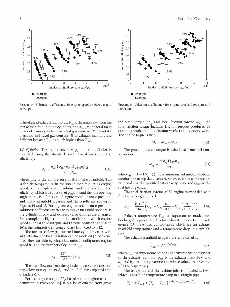
Figure 14: Volumetric efficiency for engine speeds 4500 rpm and3000 rpm.

of intake and exhaustmanifolds,𝜙𝑒in is themass flow from the

intake manifold into the cylinders, and 𝜙

𝑒out is the total massflow out from cylinder. The ideal gas constant 𝑅

𝑎of intake

manifold and ideal gas constant 𝑅 of exhaust manifold aredifferent because 𝑇emf is much higher than 𝑇imf.

3.7. Cylinder. The total mass flow 𝜙

𝑒𝑖into the cylinder is

modeled using the standard model based on volumetricefficiency:

𝜙

𝑒𝑖=

𝜂vol (𝑝imf, 𝑛𝑒, 𝛼) 𝑝imf𝑛𝑒𝑉𝑑

120𝑅

𝑎𝑇imf

, (30)

where 𝑝imf is the air pressure in the intake manifold. 𝑇imfis the air temperature in the intake manifold, 𝑛

𝑒is engine

speed, 𝑉𝑑is displacement volume, and 𝜂vol is volumetric

efficiency which is a function of 𝑝imf, 𝑛𝑒, and throttle openingangle 𝛼. 𝜂vol is a function of engine speed, throttle position,and intake manifold pressure and the results are shown inFigures 14 and 15. For a given engine and throttle position,volumetric efficiency varies with intake manifold pressure asthe cylinder intake and exhaust valve timings are changed.For example, in Figure 14, at the condition in which enginespeed is equal to 4500 rpm and throttle position is equal to26%, the volumetric efficiency varies from 0.63 to 0.42.

The fuel mass flow 𝜙

𝑒𝑓injected into cylinder varies with

air fuel ratio.The fuel mass flow can be modeled [7] with fuelmass flow variable 𝜇

𝛿which has units of milligrams, engine

speed 𝑛

𝑒, and the number of cylinder 𝑛cyl:

𝜙

𝑒𝑓=

10

−6

120

𝜇

𝛿𝑛

𝑒𝑛cyl. (31)

Themass flow out from the cylinder is the sum of the totalmass flow into cylinders 𝜙

𝑒𝑖and the fuel mass injected into

cylinders 𝜙𝑒𝑓.

For the engine torque 𝑀

𝑒, based on the engine friction

definition in reference [15], it can be calculated from gross

0.2

0.3

0.4

0.5

0.6

0.7

0.8

0.9

1

19%

30%34%

37%

45%

15%

30%

50%

55%

2000 rpm1200 rpm

2 4 6 8 10 12 14×104Intake manifold pressure pimf/pa

Volu

met

ric effi

cien

cy𝜂

vol

Figure 15: Volumetric efficiency for engine speeds 2000 rpm and1200 rpm.

indicated torque 𝑀

𝑖𝑔and total friction torque 𝑀

𝑡𝑓. The

total friction torque includes friction torques produced bypumping work, rubbing friction work, and accessory work.The engine toque is then

𝑀

𝑒= 𝑀

𝑖𝑔−𝑀

𝑡𝑓. (32)

The gross indicated torque is calculated from fuel con-sumption:

𝑀

𝑖𝑔=

30𝜙

𝑒𝑓𝑄HV𝜂𝑖𝑔

𝜋𝑛

𝑒

, (33)

where 𝜂𝑖𝑔= 1−(1/𝑟

𝛾−1

𝑐) (this assumes instantaneous adiabatic

combustion at top dead center), where 𝑟𝑐is the compression

ratio and 𝛾 is the specific heat capacity ratio, and 𝑄HV is thefuel heating value.

The total friction torque of SI engine is modeled as afunction of engine speed:

𝑀

𝑡𝑓=

𝑉

𝑑10

5

4𝜋

(𝐶

𝑓1+ 𝐶

𝑓2

𝑛

𝑒

1000

+ 𝐶

𝑓3(

𝑛

𝑒

1000

)

2

) .(34)

Exhaust temperature 𝑇exh is important to model tur-bocharged engines. Models for exhaust temperature in ref-erence [17] have two components, which are an exhaustmanifold temperature and a temperature drop in a straightpipe.

The exhaust manifold temperature is modeled as

𝑇cyl = 𝑒

𝑎cy+(𝑏cy/𝜙exh), (35)

where𝑇cyl is temperature of the fluid delivered by the cylinderto the exhaust manifold, 𝜙exh is the exhaust mass flow, and𝑎cy and 𝑏cy are tuning parameters, whose values are 7.239 and−0.005, respectively.

The temperature at the turbine inlet is modeled as (36),which is based on temperature drop in a straight pipe:

𝑇exh = 𝑇amb + (𝑇cyl − 𝑇amb) 𝑒−ℎ𝑐V𝜋𝑑pipe𝑙pipe/𝜙exh𝐶𝑝

, (36)


0 0.02 0.04 0.06 0.08 0.1 0.12400

500

600

700

800

900

1000

1100

1200

1300

ModelMeasured

Exhaust mass flow 𝜙exh (kg/s)

Exha

ust t

empe

ratu

reT

cyl(

K)

Figure 16: Model of the temperature at the turbine inlet.

where 𝑇amb is the pipe wall temperature which is equal toambient temperature, ℎ

𝑐V is the total transfer coefficient,𝑑pipe and 𝑙pipe are the diameter and length of exhaust pipe,respectively, and 𝐶

𝑝is the heat capacity. The model validated

results are shown in Figure 16. 𝑇cyl is predicted utilizing (35)and the parameters of 𝑇cyl are tuned.

4. Experiment and Simulation

All engine models above are parameterized to experimentaldata that are collected on a 2.0 L four-cylinder turbochargedSIDI engine at steady state conditions. Sensors like in-cylinder pressure sensors, k-type thermocouples, and airflow meter are equipped on the test bench. The models arevalidated at engine speeds from 1000RPM up to 4500 RPM.

The whole simulation models are implemented inSimulink according to the physical engine system, as shownin Figure 17. The parameters and coefficients of the modelsare listed in Section 3. The completed model includes inter-cooler, throttle, intake manifold, cylinder, air filter, compres-sor, turbo, turbine, and exhaust manifold.

The engine was operated at around 2200 r/min withgasoline 97#. Figures 18 and 19 show the other engines’working conditions. The throttle position was stepped from33.7% open to 45.5% open, after holding for 35 seconds,and then fell back to 38.4% open. The varying tendency ofinjection duration is almost the same.

In Figures 20–23, the simulated results are comparedto the experimental measurements. The model is able tocapture the transient dynamics and estimate the outputs withdesirable accuracy. In Figure 20, the modeled intake massflow results are a little ahead of experimental measurementsat the rising phase. After that, the model retains its goodtracking performance. The transient error is a result of theresponse time of the air mass flow transducer. In Figure 21,the model tracks the transient dynamics well at the rising

Turbo inertia

Turbine

ThrottleIntercooler

Intake manifold

Exhaust manifold

Ne

Cylinder

CompressorAir filter

Throttle

Engine speed

Pt ∗ 𝜂m

𝜔t

𝜔t

𝜔t

pem

Tem

uvgt

Wt

Tamb Tamb

Tamb

Pamb

Pamb

Pamb

Xim

Weo

Tcy

Wt

Pem

Tem

Pwrc

Pwrc

Paf

Taf Taf

Wc

Wc

Wc

Wc

Tc

Pc

TcPc

Tic

Wic

Pic

Tic

Tcy

WicWim

Wth

Wth

Wei

Weo

Pth Pth

Tth

Tim

Pim

Xim

Wim

Tim

Pim

Tth𝛼th

Pt ∗ 𝜂tmXOe

XOe

paf

pic

pamb

Figure 17: Complete control-oriented model.

0 20 40 60 80 100 120 14030

35

40

45

50

Time (s)

Thro

ttle p

ositi

on𝛼

(%)

Figure 18: Throttle position of engine operation conditions.

3.4

3.6

3.8

4

0 20 40 60 80 100 120 140Time (s)

Inje

ctio

n tim

etin

t(m

s)

Figure 19: Injection duration of engine operation conditions.


100

110

120

130

140

MeasuredModel

0 20 40 60 80 100 120 140Time (s)

Inta

ke m

ass fl

ow𝜙i

(kg/

h)

Figure 20: Measured and modeled results of intake air mass flow.

6.5

7

7.5

8

8.5

9

MeasuredModel

0 20 40 60 80 100 120 140Time (s)

Fuel

mas

s flow

𝜙f

(kg/

h)

Figure 21: Measured and modeled results of fuel mass flow.

0 50 100 1501.05

1.1

1.15

1.2

1.25

1.3

Time (s)

MeasuredModel

Boos

t pre

ssur

epb

(bar

)

Figure 22: Measured and modeled results of boost pressure.

phase, but, in stable phase, the estimation error is 0.11, about1.3%.The boost pressure and intake manifold pressure resultsshown in Figures 22 and 23 have the same characteristics withfuel mass flow.

0 50 100 150Time (s)

MeasuredModel

0.8

0.9

1

1.1

1.2

1.3

Inta

ke m

anifo

ld p

ress

urep

imf

(bar

)

Figure 23: Measured and modeled results of intake manifoldpressure.

5. Conclusions

A complete mean value model based on component sub-models has been developed and validated. The intendedapplications of the models are developments of model-basedcontrol strategies and system analysis. Several submodelswere described and novel models for compressor flow andcompressor efficiency were developed. The accuracy of thenew compressor model has an average error of 0.12%,which is a significant improvement over conventional map-ping approaches. The experimental results confirm that thedeveloped model is capable of tracking transient dynamics.Compared to the conventional lookup table approach, ourvalidation results show that transient dynamics error can beimproved significantly through using the model from thiswork.

Conflict of Interests

The authors declare that there is no conflict of interestsregarding the publication of this paper.

Acknowledgments

The authors would like to acknowledge Dr. Patrick Gorzelicof the University of Michigan (Ann Arbor) for the dis-cussions and suggestions about the models. This project issupported by National Natural Science Foundation of China(no. 51475151), China Scholarship Council Foundation (no.2012-3022), and Hunan University Young Teachers SponsorProject.

References

[1] G. A. Lavoie, J. Martz,M.Wooldridge, andD. Assanis, “Amulti-mode combustion diagram for spark assisted compression


ignition,” Combustion and Flame, vol. 157, no. 6, pp. 1106–1110,2010.

[2] P. Gorzelic, P. Shingne, J. Martz, and G. A. Stefanopoulou, “Alow-order HCCI model extended to capture SI-HCCI modetransition data with two-stage cam switching,” in Proceedingsof the ASME Dynamic Systems and Control Conference, SanAntonio, Tex, USA, October 2014.

[3] E. Hellstrom, J. Larimore, S. Jade, A. G. Stefanopoulou, and L.Jiang, “Reducing cyclic variability while regulating combustionphasing in a four-cylinder HCCI engine,” IEEE Transactions onControl Systems Technology, vol. 22, no. 3, pp. 1190–1197, 2014.

[4] P. Moraal and I. Kolmanovsky, “Turbocharger modeling forautomotive control applications,” in Proceedings of the SAEWorld Congress & Exhibition, Detroit, Mich, USA, March 1999.

[5] L. Eriksson, “Modeling and control of turbocharged SI and DIengines,” Oil & Gas Science and Technology, vol. 62, no. 4, pp.523–538, 2007.

[6] L. Kocher, E. Koeberlein, K. Stricker, D. G. van Alstine, B.Biller, and G. M. Shaver, “Control-oriented modeling of dieselengine gas exchange,” in Proceedings of the American ControlConference (ACC ’11), pp. 1555–1560, San Francisco, Calif, USA,June-July 2011.

[7] M. Taburri, F. Chiara, M. Canova, and Y.-Y. Wang, “A model-basedmethodology to predict the compressor behaviour for thesimulation of turbocharged engines,” Proceedings of the Insti-tution of Mechanical Engineers, Part D: Journal of AutomobileEngineering, vol. 226, no. 4, pp. 560–574, 2012.

[8] M. Santillo and A. Karnik, “Model Predictive Controller designfor throttle and wastegate control of a turbocharged engine,” inProceedings of the American Control Conference (ACC ’13), pp.2183–2188, IEEE, Washington, DC, USA, June 2013.

[9] D. Malkhede and B. Seth, “State feedback speed controller forturbocharged diesel engine and its robustness,”World Academyof Science, Engineering and Technology, vol. 75, pp. 119–125, 2013.

[10] R. Salehi, M. Shahbakhti, A. Alasty, and G. R. Vossoughi,“Control oriented modeling of a radial turbine for a tur-bocharged gasoline engine,” in Proceedings of the AmericanControl Conference (ACC ’13), pp. 5207–5212, Washington, DC,USA, June 2013.

[11] N. Watson and M. S. Janota, Turbocharging the Internal Com-bustion Engine, Macmillan, Basingstoke, UK, 1982.

[12] P. Moraal and I. Kolmanovsky, “Turbocharger modeling forautomotive control applications,” in Proceedings of the SAEInternational Congress & Exposition, Paper no. 1999-01-0908,pp. 1–14, Detroit, Mich, USA, March 1999.

[13] Y. A. Cengel,Heat Transfer: A Practical Approach,McGraw-Hill,New York, NY, USA, 2002.

[14] L. Eriksson, L. Nielsen, J. Brugard, J. Bergstrom, F. Pettersson,and P. Andersson, “Modeling of a turbocharged SI engine,”Annual Reviews in Control, vol. 26, no. 1, pp. 129–137, 2002.

[15] J. B. Heywood, Internal Combustion Engine Fundamentals,McGraw-Hill, New York, NY, USA, 1988.

[16] M. Nyberg and L. Nielsen, “Model based diagnosis for theair intake system of the SI-engine,” in Proceedings of the SAEInternational Congress & Exposition, Paper no. 970209, Detroit,Mich, USA, February 1997.

[17] L. Eriksson, “Mean value models for exhaust system tempera-ture,” in Proceedings of the SAE World Congress & Exhibition,Paper no. 2002-01-0374, Detroit, Mich, USA, March 2002.

Submit your manuscripts athttp://www.hindawi.com

Hindawi Publishing Corporationhttp://www.hindawi.com Volume 2014

Inorganic ChemistryInternational Journal of

Hindawi Publishing Corporation http://www.hindawi.com Volume 2014

International Journal ofPhotoenergy


Carbohydrate Chemistry

International Journal of


Journal of

Chemistry


Advances in

Physical Chemistry

Hindawi Publishing Corporationhttp://www.hindawi.com

Analytical Methods in Chemistry

Journal of

Volume 2014

Bioinorganic Chemistry and ApplicationsHindawi Publishing Corporationhttp://www.hindawi.com Volume 2014

SpectroscopyInternational Journal of


The Scientific World JournalHindawi Publishing Corporation http://www.hindawi.com Volume 2014

Medicinal ChemistryInternational Journal of


Chromatography Research International


Applied ChemistryJournal of



Theoretical ChemistryJournal of


Journal of

Spectroscopy

Analytical ChemistryInternational Journal of


Journal of


Quantum Chemistry


Organic Chemistry International

ElectrochemistryInternational Journal of

Hindawi Publishing Corporation http://www.hindawi.com Volume 2014


CatalystsJournal of

Research on Control-Oriented Modeling for Turbocharged SI and DI ...

Documents

Transcript of Research on Control-Oriented Modeling for Turbocharged SI and DI ...