Can risk explain the profitability of technical trading incurrency markets?

FEDERAL RESERVE BANK OF ST. LOUISResearch Division

P.O. Box 442St. Louis, MO 63166

RESEARCH DIVISONWorking Paper Series

Yuliya Ivanova,Christopher J. Neely

andPaul A. Weller

Working Paper 2014-033E

11/01/2016

The views expressed are those of the individual authors and do not necessarily reflect official positions of the FederalReserve Bank of St. Louis, the Federal Reserve System, or the Board of Governors.

Federal Reserve Bank of St. Louis Working Papers are preliminary materials circulated to stimulate discussion andcritical comment. References in publications to Federal Reserve Bank of St. Louis Working Papers (other than anacknowledgment that the writer has had access to unpublished material) should be cleared with the author or authors.

 

 

 

Can risk explain the profitability of technical trading in currency markets?* 

 

 

 

 

 Yuliya Ivanova 

 

Quantitative Associate, 

Promontory Financial 

Group  

Christopher J. Neely 

 

Assistant Vice President, 

Federal Reserve Bank of St. 

Louis  

Paul Weller 

 

John F. Murray Professor 

of Finance Emeritus,  

The University of Iowa 

 

 

 

 

May 6, 2018 

 

 

 

 

 

JEL Codes:  F31, G11, G12, G14 

 

Keywords: Exchange rate; Technical analysis; Technical trading; Efficient 

markets hypothesis; Risk; Stochastic Discount Factor; Adaptive markets 

hypothesis; Carry trade. 

 

 

* Chris Neely is the corresponding author. Federal Reserve Bank of St. Louis, Box 442, St. Louis, MO 63166. 

e‐mail: neely@stls.frb.org; phone: +1‐314‐444‐8568; fax: +1‐314‐444‐8731. We thank seminar participants at 

the Federal Reserve Bank of St. Louis, Macquarie University, and the Midwest Finance Association Meetings 

for helpful comments. The usual disclaimer applies. The views expressed in this paper are those of the 

authors and do not reflect those of the Federal Reserve Bank of St. Louis, the Federal Reserve System or the 

Promontory Financial Group. 

 

 

 

 Abstract

Academic studies show that technical trading rules would have earned substantial excess 

returns over  long periods  in  foreign exchange markets. However,  the approach  to risk 

adjustment has typically been rather cursory. We examine the ability of a wide range of 

models: CAPM,  quadratic CAPM, downside  risk CAPM, C‐CAPM, Carhart’s  4‐factor 

model, an extended C‐CAPM with durable consumption, Lustig‐Verdelhan (LV) factors, 

volatility, skewness and  liquidity  to explain  these  technical  trading  returns. No model 

plausibly accounts for technical profitability in the foreign exchange market.  

 

 

   

1

  Introduction  

 

It is a stylized fact that excess returns for currency‐related trading strategies, such 

as technical trading rules and the carry trade, are weakly correlated with traditional risk 

factors,  such  as  the  CAPMʹs  equity market  factor.  This  is  interpreted  to  imply  that 

significantly positive excess returns constitute evidence of market inefficiency. But, as has 

been emphasized by Fama (1970), any such test of market efficiency is inevitably a joint 

test  of  efficiency  and  of  the  particular  asset  pricing  model  chosen.  An  apparent 

inefficiency may  simply  be  the  result  of  having  selected  a misspecified model.  This 

consideration has spurred the search for other plausible risk factors that are able to explain 

the observed anomalous returns. 

This search has focused almost exclusively on excess returns  to  the carry  trade, 

and there are a number of recent studies that propose a variety of risk factors for carry 

trade portfolios. These risk factors include consumption growth (Lustig and Verdelhan, 

2007), a forward premium slope factor (Lustig, Roussanov, and Verdelhan, 2011), global 

exchange  rate  volatility  (Menkhoff,  Sarno,  Schmeling,  and  Schrimpf,  2012a),  and 

skewness (Rafferty, 2012). 

These  recently  proposed  currency  risk  factors  succeed  to  varying  degrees  in 

explaining  the  returns  to  a  cross‐section  of  carry  trade  portfolios.  Nevertheless,  the 

economic case for these factors would be more compelling if they could also explain excess 

returns  for other  investment  strategies, beyond  the  carry  trade  (Burnside,  2012). Such 

explanatory ability would allay data‐mining concerns and better establish the economic 

relevance  of  the  newly  proposed  currency  risk  factors.  If  new  risk  factors  cannot 

2

adequately account for the returns to technical strategies, then this implies that the excess 

returns provide evidence of market inefficiency.  

Technical analysis constitutes a long‐standing puzzle in foreign exchange returns, 

one that has received less attention than the carry trade despite a well‐documented history 

of success. A series of studies in the 1970s and 1980s demonstrated that technical analysis 

produced abnormal returns in foreign exchange markets (Dooley and Shafer (1976, 1984), 

Logue and Sweeney (1977), and Cornell and Dietrich (1978)).  Although academics were 

initially very skeptical of these findings, the positive results of Sweeney (1986) and Levich 

and Thomas (1993) helped convince the profession of the robustness of this puzzle. Allen 

and Taylor (1990) and Taylor and Allen (1992) confirmed this shift in outlook by surveying 

practitioners to establish that foreign exchange traders commonly used technical analysis. 

Later research looked at the usefulness of commonly used technical patterns (Osler and 

Chang (1995)) and considered reasons for time variation in profitability (Neely, Weller, 

and  Ulrich  (2009)). Menkhoff  and  Taylor  (2007)  provide  an  excellent  survey  of  the 

literature. Recently, Hsu, Taylor, and Wang (2016) conduct a large scale investigation of 

technical  analysis,  concluding  that  technical methods  have  significant  economic  and 

statistical predictive power for both developed and emerging currencies.  

These studies have established that technical analysis would have been profitable 

for long periods for a wide variety of currencies, but no study has definitively explained 

this profitability as the return to one or more risk factors. However, the risk adjustment 

procedures have focused almost exclusively on applications of the CAPM. The risk factors 

that have explained carry‐trade returns — and other anomalies — are natural candidates 

3

to explain  the returns  to  technical analysis. A study of  the extent  to which  factors  that 

explain the carry trade also explain the returns to technical analysis will shed light on both 

the source of technical returns and the plausibility of the factors.  If the carry trade factors 

explain the returns to technical analysis, then it is very likely that they are truly sources of 

undiversifiable  risk. On  the  other  hand,  if  the  carry‐trade  factors  fail  to  explain  the 

technical returns, it suggests that the factors merit continued scrutiny and that risk is less 

likely to be the source of the technical returns.  

In this spirit, the present paper investigates the ability of a wide variety of currency 

risk  factors,  some of which have been  shown  recently  to have  substantial explanatory 

power for carry trade returns, to explain excess returns for a group of ex ante technical 

portfolios developed in Neely and Weller (2013). These portfolios are based on a variety 

of popular  technical  indicators  that  the academic  literature has  studied and provide a 

realistic picture of  returns  for  trend‐following practitioners. We adjust  returns  for  risk 

with  the  following models: CAPM, quadratic CAPM, downside risk CAPM, C‐CAPM, 

Carhart’s 4‐factor model, an extended C‐CAPM with durable consumption and market 

return, Lustig‐Verdelhan (LV) factors, global FX volatility, global FX skewness, skewness 

in unemployment  and FX  liquidity. We  find  that none  of  the proposed  currency  risk 

factors  can explain  technical portfolio  returns. The  risk  factors  identified  in  the  recent 

literature  thus do not appear  to be  relevant  for an  important class of portfolios  in  the 

currency  space. We highlight  the dimensions  along which  the new  risk  factors  fail  to 

account for the behavior of technical portfolios. The inadequacies of extant currency risk 

factors highlight the challenges in explaining technical portfolio returns. 

4

  The rest of the paper is organized as follows. We first describe the construction of 

currency portfolios. We then describe the different currency risk factors that we consider 

and the econometric methodology. Our empirical results follow. 

Trading Rules and Data 

The goal of our paper is to examine whether recent advances in risk‐adjustment 

can explain the seemingly very strong performance of traditional technical trading rules 

in  foreign  exchange markets.   To do  so, we must  construct  such  returns  in  a manner 

consistent with the literature that has established their profitability.  We would like our 

trading rules to represent those that the academic literature has investigated but also to 

be chosen dynamically, to exploit changing patterns in adaptive markets. In order to do 

so, we follow Neely and Weller (2013) who dynamically constructed portfolio strategies 

from an underlying pool of  frequently studied rules— 7  filter rules, 3 moving average 

rules, 3 momentum rules, and 3 channel rules— on 19 dollar and 21 cross exchange rates.2 

These  rule  sets are among  the most  commonly  studied  in  the academic  literature and 

therefore  are  appropriate  to  study  the  puzzle.  Although  there  are many  reasonable 

variations  on  rule  selection,  the  robustness  of  academic  results  on  technical  trading 

profitability leads us to believe that reasonable perturbations are unlikely to substantially 

change inference for risk adjustment. The rules in the present paper differ in one notable 

respect  from  those  in Neely and Weller  (2013):  to  isolate  the determinants of  technical 

2 Dooley and Shafer (1984) and Sweeney (1986) look at filter rules; Levich and Thomas (1993) look at filter and 

moving average  rules;  Jegadeesh and Titman  (1993) consider momentum  rules  in equities, citing Bernard 

(1984) on the topic; and Taylor (1994) tests channel rules, for example.   

5

trading rules, the present paper does not include carry trade returns among the rules.   

All of the bilateral rules borrow in one currency and lend in the other to produce 

excess  returns. We will  first  describe  the  types  of  trading  rules  before  detailing  the 

dynamic rebalancing procedure for currency trading strategies.  

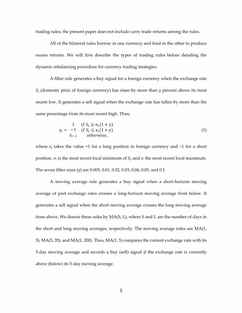
A filter rule generates a buy signal for a foreign currency when the exchange rate 

 (domestic price of foreign currency) has risen by more than y percent above its most 

recent low. It generates a sell signal when the exchange rate has fallen by more than the 

same percentage from its most recent high. Thus,  

11

1 1

,                 (1) 

where   takes  the value +1  for a  long position  in  foreign  currency and –1  for a  short 

position. nt is the most recent local minimum of  and xt the most recent local maximum. 

The seven filter sizes (y) are 0.005, 0.01, 0.02, 0.03, 0.04, 0.05, and 0.1.  

A moving  average  rule  generates  a  buy  signal when  a  short‐horizon moving 

average of past  exchange  rates  crosses a  long‐horizon moving average  from below.  It 

generates a sell signal when the short moving average crosses the long moving average 

from above. We denote these rules by MA(S, L), where S and L are the number of days in 

the short and long moving averages, respectively. The moving average rules are MA(1, 

5), MA(5, 20), and MA(1, 200). Thus, MA(1, 5) compares the current exchange rate with its 

5‐day moving average and  records a buy  (sell) signal  if  the exchange  rate  is currently 

above (below) its 5‐day moving average.  

6

Our momentum rules take a long (short) position in an exchange rate when the n‐

day cumulative return is positive (negative). We consider windows of 5, 20 and 60 days 

for the momentum rules.3  

A channel rule takes a  long (short) position  if the exchange rate exceeds (is  less 

than)  the maximum  (minimum)  over  the  previous  n  days  plus  (minus)  the  band  of 

inaction (x). Thus, 

11

, , … 1 , , … 1

,                          (2) 

We set n to be 5, 10, and 20, and x to be 0.001 for all channel rules. 

We  apply  these  16  bilateral  rules —7  filter  rules,  3 moving  average  rules,  3 

momentum rules, and 3 channel rules— to daily data on 19 dollar and 21 cross exchange 

rates,  listed  in Table 1. The series for the DEM was spliced with that for the EUR after 

January  1,  1999. For  simplicity we  refer  to  this  series  throughout  as  the EUR. Not  all 

exchange rates are tradable throughout the sample. Table 1 details the dates on which we 

permit trading in each exchange rate.  

In any study of trading performance—especially when using exotic currencies—it 

is  important  to pay  close  attention  to  transaction  costs. Rules  and  strategies  that may 

3 Menkhoff,  Sarno,  Schmeling,  and  Schrimpf  (2012b)  empirically  compare  several moving  average  rules, 

which  they  consider  to be benchmark  technical  rules, with  cross‐sectional, momentum  rules on monthly 

currency data and argue that the two types of rules behave quite differently. We obtained the monthly returns 

constructed by Menkhoff et al. (2012b) from the Journal of Financial Economics website and investigated the 

relation between those rules and the monthly returns to our portfolios. The Menkhoff et al. (2012b) Mom(1,1) 

rule has the highest correlations with our portfolio returns, having a correlation of 0.23 with p1 returns (see 

below for definition). Most correlations between the cross‐section momentum and our technical rules were 

lower, some as low as 0. The median correlation was 0.13. Therefore, we concur with Menkhoff et al.’s (2012b) 

conclusion that monthly cross‐sectional rules are only weakly related to traditional technical rules. 

7

appear to be profitable when such costs are ignored turn out not to be once the appropriate 

adjustments have been made. We  follow  the methods  in Neely and Weller  (2013) and 

calculate transactions costs using historical estimates for such costs in the distant past and 

fractions  of  Bloomberg  spreads  for  dates  after which    such    spreads were  available. 

Appendix A of Neely and Weller (2013) details these calculations. 

Dynamic Trading Strategies 

We would  like  to  construct dynamic  strategies  to mimic  the actions of  foreign 

exchange  traders who backtest potential  rules on historical data  to determine  trading 

strategies.  Accurately modeling  potential  trading  returns  provides  the most  realistic 

environment for assessing whether risk adjustment explains such returns. We therefore 

employ  the previously described  trading rules  to construct dynamic  trading strategies. 

Each trading strategy uses rules and exchange rate combinations that vary over time. 

We construct dynamic trading strategies as follows:   

1. We apply the 16 bilateral rules to all tradable exchange rates at each point 

in the sample, calculating the historical return statistics for each exchange rate‐rule pair at 

each point.  There is a maximum of (16*40=) 640 exchange rate‐rules on any given day, but 

missing data for some exchange rates often leave fewer than half that number of currency‐

rule pairs. 

2. Starting  500 days  into  the  sample, we  evaluate  the  Sharpe  ratios  of  all 

exchange rate‐rule pairs with at least 250 days of data since the beginning of the respective 

samples. We then sort the rate‐rule pairs by their ex post Sharpe ratios, ranking the rate‐

8

rule  pairs  by  Sharpe  ratio  from  1  to  640.   We  then measure  the  performance  of  the 

strategies over the next 20 days. 

3. Every 20 business days, we evaluate, sort and rank all available rate‐rule 

pairs using the complete sample of data available to that point. Thus, the returns on the 

top‐ranked strategy pair will be generated by a given trading rule applied to a particular 

exchange rate for a minimum of 20 days, at which point it may (or may not) be replaced 

by another rule applied to the same or a different currency.4 

Although we  select  the  rate‐rule  pairs  for  the  dynamic  strategies  based  upon 

historical performance, as described above, we evaluate the strategies’ performances after 

they are selected.  That is, all return performance statistics in this paper are for strategies 

that were chosen ex ante and are thus implementable in real time.   

Currency portfolios 

As  is  customary  in  the  related  asset‐pricing  literature,  we  examine  the  risk‐

adjustment of technical trading rules in the following way: Using strategies 1 to 300 as test 

assets, we form 12 equally weighted portfolios of 25 strategies per portfolio. Thus portfolio 

p1  at  time  t  consists  of  the  25  currency‐rule pairs with  Sharpe  ratios  ranked  1  to  25. 

Portfolio p2 consists of the 25 currency‐rule pairs with Sharpe ratios ranked 26 to 50, and 

so on. The makeup of  the portfolios of currency‐rule pairs may change  from period  to 

period with ex post Sharpe ratio rankings. 

4 We emphasize that our strategies do not use 20‐day holding periods for positions. The holding periods for 

the trading rules are always 1‐day. Each strategy, however, can switch rule/exchange rate combinations every 

20‐days. Within each 20‐day period, the rule can instruct the strategy to switch back and forth between long 

and short positions in the particular exchange rate.  

9

Figure  1  shows  the  spread  in  excess  return,  standard deviation,  Sharpe  ratios, 

skewness and kurtosis over the 12 portfolios. The top panel shows that all 12 portfolios 

have positive excess returns, generally declining as one goes from p1 (4.35% per annum) 

to p12 (0.69% per annum).  The second panel shows that the high ranked portfolios also 

tend to have more volatile returns, though the relation is not as steep as for returns. The 

third panel confirms this: ex post Sharpe ratios are higher for the portfolios with higher 

ex ante rankings, ranging from 0.82 for p1 to 0.16 for p12. 

Theoretical framework 

To provide a general framework within which to measure risk exposure we need 

to characterize equilibrium in the foreign exchange market. We assume the existence of a 

representative,  US‐based  investor  and  introduce  a  stochastic  discount  factor  (SDF), 

that prices payoffs in dollars.5 It represents a marginal rate of substitution between 

present and future consumption in different states of the world. The first order conditions 

for utility maximization subject to an intertemporal budget constraint imply that any asset 

return   must satisfy  

|  = 1                                 (3) 

where   denotes the information available to the investor at time t. Varying assumptions 

about the content of   produce the different categories of market efficiency advanced by 

Fama (1970). Since we are modeling the risk exposure of technical trading rules we will 

be exclusively concerned with weak‐form efficiency, in which the information set   contains 

5 Although we motivate the SDF framework with a representative  investor, much weaker assumptions are 

sufficient. In particular, absence of arbitrage implies the existence of a SDF framework, as in equation (3).  

10

only past prices.   

Equation (3) implies that the risk‐free asset return   is given by     

   =   .                (4) 

Using (3), (4) and the definition of covariance, it follows that  

|  =   ‐ ,

.             (5) 

That is, the excess return to any asset, and by extension any trading strategy, will 

be proportional to the covariance of the asset return with the SDF. 

The  implication  for  technical  trading  strategies  that  take  positions  in  foreign 

currencies  based  on  past  prices  is  then  straightforward.  Positive  excess  returns  to  a 

strategy  are  consistent  with  market  efficiency  only  if  those  excess  returns  covary 

negatively with the SDF. This then raises the question of how to model the SDF and how 

to test whether equation (5) or some variant explains returns.  

There are potentially several ways in which one could test the extent to which the 

SDF framework can explain excess returns to the trading rules.  The most direct would be 

to model the SDF,  , in (3) with a specific utility function and calibrated parameters 

and test whether the errors from (3) are mean zero. Alternatively, one could estimate the 

parameters of   with some nonlinear optimization method, such as  the generalized 

method of moments (GMM), and test the overidentifying restrictions. Finally, one could 

linearize the SDF,  , with a Taylor series expansion, estimate a linear time series or a 

return‐beta model and evaluate whether the risk factors explain the expected returns. The 

next subsections describe those testing procedures.  

11

Testing a Calibrated SDF 

Our  initial approach  to risk adjustment will be  to  follow Lustig and Verdelhan 

(2007)  in  using  an  extended  version  of  the  C‐CAPM  that  employs  Yogo’s  (2006) 

representative agent framework with Epstein‐Zin preferences over durable consumption 

 and nondurable consumption,  . Utility is given by 

1 , ⁄ ⁄ ⁄⁄

              (6) 

where   is the time discount factor,   is a measure of risk aversion,   is the elasticity of 

intertemporal substitution in consumption, and  1 1 1⁄⁄ . 

The one‐period utility function is given by 

, 1 ⁄ ⁄ ⁄⁄                           (7) 

where   is  the weight  on  durable  consumption  and   is  the  elasticity  of  substitution 

between durable and nondurable  consumption. Yogo  (2006)  shows  that  the  stochastic 

discount factor takes the form 

⁄ ⁄

⁄

⁄⁄

,⁄

,                           (8) 

where   1⁄ ⁄⁄

and  ,  is the market portfolio return. 

This model, the Epstein‐Zin durable consumption CAPM (EZ‐DCAPM), nests two 

other models of interest: the durable consumption CAPM (DCAPM) and the CCAPM. The 

DCAPM  holds  under  the  restriction 1⁄ .  The CCAPM  holds  if,  in  addition,  one 

imposes  . The stochastic discount factor in (8) satisfies the familiar Euler equation in 

(3).  

12

To  initially  assess  the performance of  these models, we  carry out a  calibration 

exercise  similar  to  that  in  Lustig  and Verdelhan  (2007). We  choose  parameter  values 

identified  in Yogo  (2006):  0.023, 0.802, 0.700. Then we use  sample data on 

durable and non‐durable consumption and the return on the market portfolio to generate 

pricing  errors,  , where R  is  the  excess  return  to portfolio pi,  and  i 

1,… ,12 . 6  The  coefficient  of  relative  risk  aversion   is  chosen  to minimize  the  sum  of 

squared pricing  errors  in  the EZ‐DCAPM. Appendix B details  the  construction of  the 

variables used in this paper.  

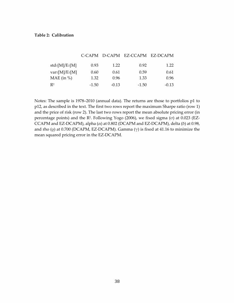
Table 2 presents these results. All models clearly perform very poorly; the   is 

negative  in every case.7 The maximum Sharpe ratios and price of risk are substantially 

different from those reported in Table 4 of Lustig and Verdelhan (2007). Since their test 

assets are currency portfolios sorted according  to  interest differential we would expect 

these numbers to be similar. The portfolios with the highest returns have negative betas; 

p1 has a beta of ‐1.97. This implies that the portfolio return covaries positively with M. 

Since M is high in bad times when marginal utility is high and consumption is low, these 

portfolios  act  as  consumption hedges  and would be  expected  to  earn negative  excess 

returns according to the theory. 

6 Recall that portfolios p1 to p12 each consist of 25 currency‐rule pairs, ranked every 20 days by ex ante Sharpe 

ratio. p1 contains strategies 1 to 25; p2 contains strategies 26 to 50 and so on.  7 The R2 can be negative because we are assessing the predictive value of a calibrated, ex ante model, not the 

predictive value of a model estimated to maximize the R2. 

13

Linear Factor Models 

Researchers often linearize the SDF with a first order Taylor approximation and 

then assess the model’s fit of the data with that linear system.  Although it is not clear how 

well the linear model approximates the SDF, this procedure makes estimation somewhat 

easier and is consistent with the literature.  

Therefore, we consider the class of linear SDFs that take the form 

                  (9) 

where   is a scalar,  is a  1 vector of parameters and   is a  1 vector of demeaned 

factors that explain asset price returns. Then the constant   in (9) is not identified, and we 

can  normalize  it  to  unity.8  The  SDF must  also  price  portfolios  of  excess  trading  rule 

returns,  , in which case equation (3) implies that    

  | 0                (10) 

The unconditional version of (10) is  

1 0               (11) 

from which it follows that  

Σ ∙ Σ          (12) 

where Σ  is the factor covariance matrix,  Σ  is a  1 vector of coefficients in 

a regression of   on   and  Σ  is a  1 vector of factor risk premia.  

The model (12) is a return‐beta representation. It implies that an asset’s expected 

return is proportional to its covariance with the risk factors.  The betas are defined as the 

8 For any pair, {a, b}, such that  0, any {ca, cb} where c is a real constant would also satisfy the 

equation because   0. Therefore, only the ratio b/a matters and one can normalize a to 1 or to 

any other constant.  

14

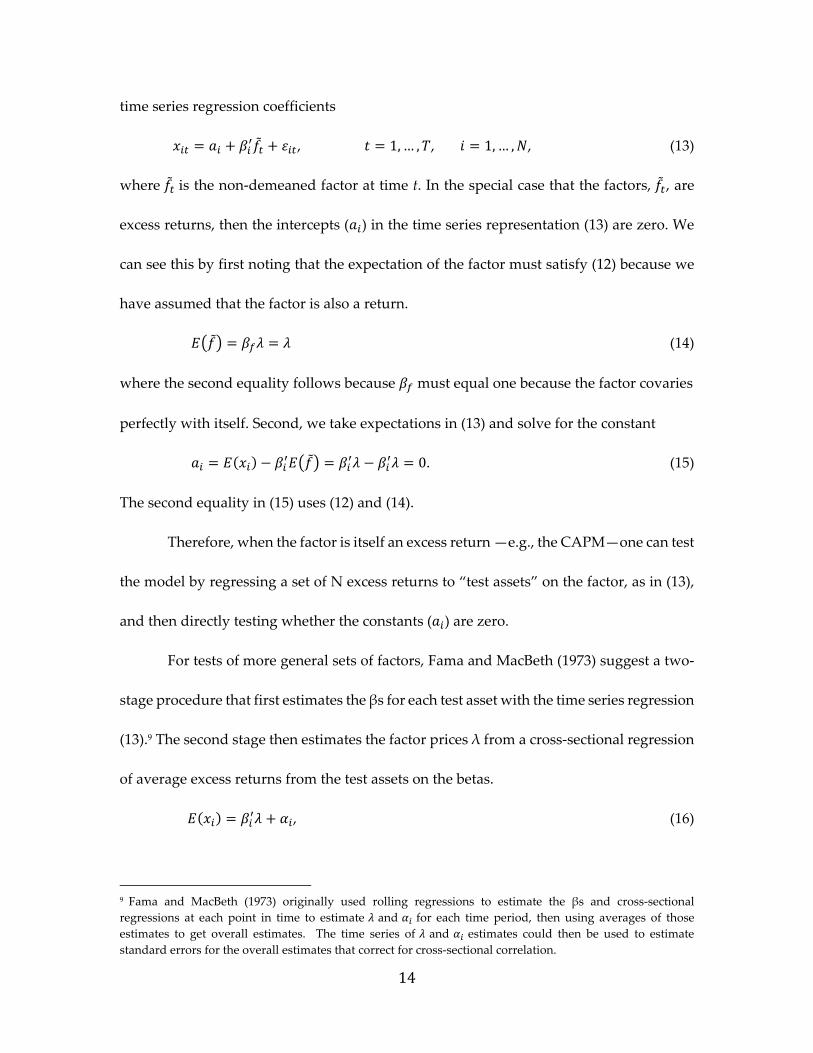
time series regression coefficients  

,    1,… , ,  1,… , ,           (13) 

where   is the non‐demeaned factor at time t. In the special case that the factors,  , are 

excess returns, then the intercepts ( ) in the time series representation (13) are zero. We 

can see this by first noting that the expectation of the factor must satisfy (12) because we 

have assumed that the factor is also a return.  

                (14) 

where the second equality follows because   must equal one because the factor covaries 

perfectly with itself. Second, we take expectations in (13) and solve for the constant  

0.           (15) 

The second equality in (15) uses (12) and (14). 

Therefore, when the factor is itself an excess return —e.g., the CAPM—one can test 

the model by regressing a set of N excess returns to “test assets” on the factor, as in (13), 

and then directly testing whether the constants ( ) are zero.  

For tests of more general sets of factors, Fama and MacBeth (1973) suggest a two‐

stage procedure that first estimates the βs for each test asset with the time series regression 

(13).9 The second stage then estimates the factor prices λ from a cross‐sectional regression 

of average excess returns from the test assets on the betas.  

,                 (16) 

9  Fama  and  MacBeth  (1973)  originally  used  rolling  regressions  to  estimate  the  βs  and  cross‐sectional 

regressions  at  each point  in  time  to  estimate   and   for  each  time period,  then using  averages of  those 

estimates  to  get  overall  estimates.   The  time  series  of   and   estimates  could  then  be used  to  estimate 

standard errors for the overall estimates that correct for cross‐sectional correlation.  

15

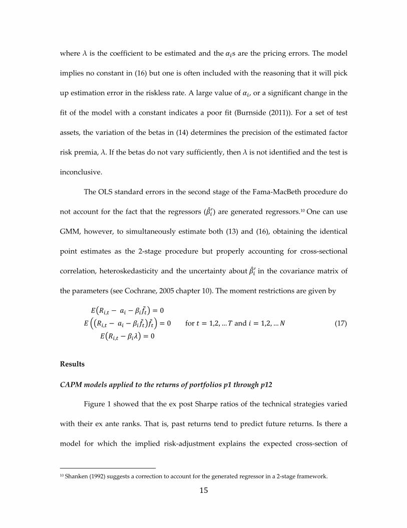
where λ  is the coefficient to be estimated and the  s are the pricing errors. The model 

implies no constant in (16) but one is often included with the reasoning that it will pick 

up estimation error in the riskless rate. A large value of  , or a significant change in the 

fit of  the model with a constant  indicates a poor  fit  (Burnside  (2011)). For a set of  test 

assets, the variation of the betas in (14) determines the precision of the estimated factor 

risk premia, λ. If the betas do not vary sufficiently, then λ is not identified and the test is 

inconclusive.  

The OLS standard errors in the second stage of the Fama‐MacBeth procedure do 

not account  for  the  fact  that  the regressors  ( ) are generated regressors.10 One can use 

GMM, however,  to simultaneously estimate both  (13) and  (16), obtaining  the  identical 

point  estimates  as  the  2‐stage  procedure  but  properly  accounting  for  cross‐sectional 

correlation, heteroskedasticity and  the uncertainty about   in  the covariance matrix of 

the parameters (see Cochrane, 2005 chapter 10). The moment restrictions are given by 

, 0

, 0

, 0

     for  1,2, …  and  1,2, …                            (17) 

Results 

CAPM models applied to the returns of portfolios p1 through p12  

Figure 1 showed that the ex post Sharpe ratios of the technical strategies varied 

with  their ex ante ranks. That  is, past returns  tend  to predict  future returns.  Is  there a 

model  for  which  the  implied  risk‐adjustment  explains  the  expected  cross‐section  of 

10 Shanken (1992) suggests a correction to account for the generated regressor in a 2‐stage framework.  

16

returns? 

As a benchmark we first look at whether the CAPM can explain the excess returns 

to the 12 portfolios, p1‐p12, which consist of strategies 1‐25, 26‐50, … 276‐300, respectively. 

The model has a single factor, the market excess return, and so we consider the following 

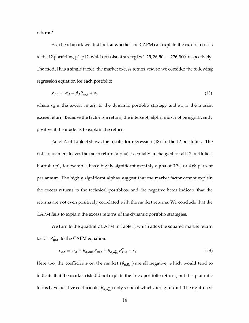
regression equation for each portfolio:  

, ,                                (18)  

where   is  the  excess  return  to  the dynamic portfolio  strategy  and   is  the market 

excess return. Because the factor is a return, the intercept, alpha, must not be significantly 

positive if the model is to explain the return.  

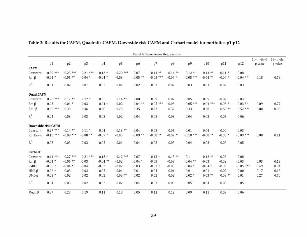
Panel A of Table 3 shows the results for regression (18) for the 12 portfolios.  The 

risk‐adjustment leaves the mean return (alpha) essentially unchanged for all 12 portfolios. 

Portfolio p1, for example, has a highly significant monthly alpha of 0.39, or 4.68 percent 

per annum. The highly significant alphas suggest that the market factor cannot explain 

the  excess  returns  to  the  technical portfolios,  and  the negative betas  indicate  that  the 

returns are not even positively correlated with the market returns. We conclude that the 

CAPM fails to explain the excess returns of the dynamic portfolio strategies. 

We turn to the quadratic CAPM in Table 3, which adds the squared market return 

factor  ,   to the CAPM equation. 

, , , , ,           (19) 

Here  too,  the  coefficients on  the market  ( ,  are all negative, which would  tend  to 

indicate that the market risk did not explain the forex portfolio returns, but the quadratic 

terms have positive coefficients ( ,  only some of which are significant. The right‐most 

17

columns show  that  these coefficients  jointly differ  from zero and  from each other. The 

positive  ,  values suggest that market volatility influences dynamic technical portfolio 

returns.  Menkhoff,  Sarno,  Schmeling  and  Schrimpf  (2012a)  document  a  similar 

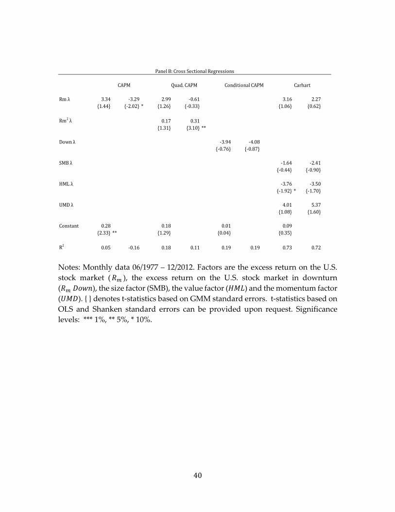
phenomenon for carry trade returns. When the constant is included in the cross‐sectional 

regression, the R2 rises from 0.11 to 0.18 but the constant is not statistically significant (see 

Panel B, Table 3).  The price of risk for the quadratic market return is 0.31 and statistically 

significant. This  is not consistent with the theoretical expectation of a negative price of 

risk, however, which leads us to conclude that the quadratic CAPM cannot explain the 

excess returns of the dynamic portfolio strategies. 

Another variant on the CAPM analyzed in a recent paper by Lettau, Maggiori and 

Weber (2014) has had considerable success in explaining returns to the carry trade. They 

construct a factor which is designed to capture the possibility that investors are concerned 

specifically about downside risk in the stock market. They follow the approach of Ang, 

Chen and Xing (2006) in allowing the price of risk and the beta of currency portfolios to 

vary  conditional  on  the  return  on  the  market.  They  call  the  underlying  model  the 

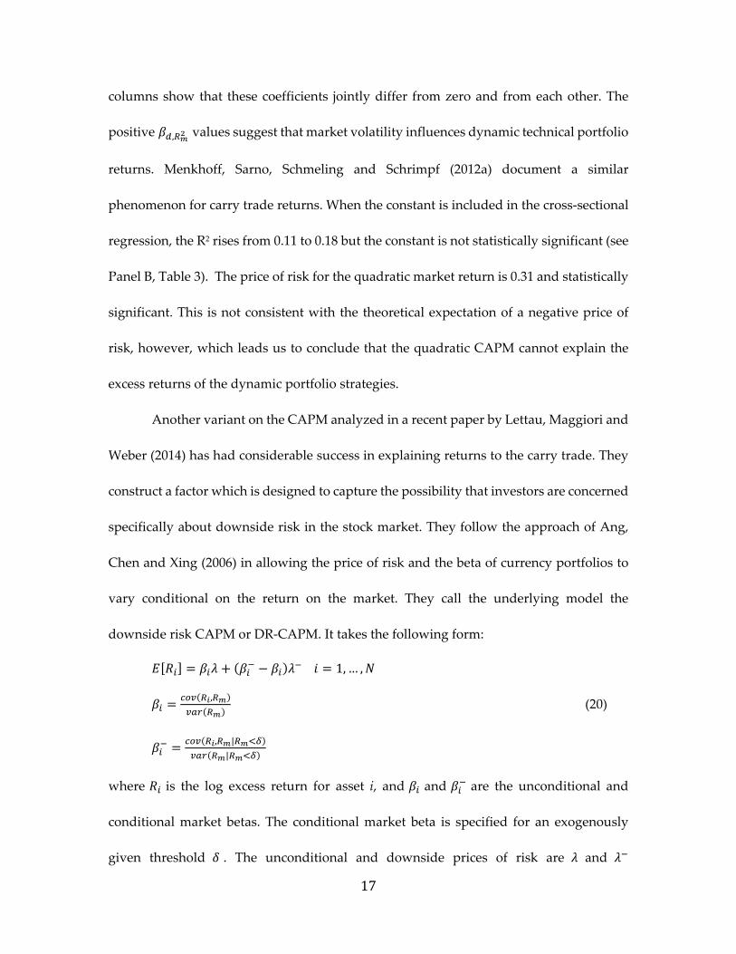
downside risk CAPM or DR‐CAPM. It takes the following form: 

1, … ,    

,                  (20) 

, |

|   

where   is  the  log  excess  return  for  asset  i,  and   and   are  the unconditional  and 

conditional market betas. The  conditional market beta  is  specified  for an exogenously 

given  threshold  .  The  unconditional  and  downside  prices  of  risk  are   and   

18

respectively. We follow Lettau, Maggiori and Weber (2014) in defining a down state to be 

one where  the  contemporaneous market  return  is more  than  one  standard  deviation 

below its sample average. The unconditional price of risk is also set to the average market 

return following Lettau, Maggiori and Weber (2014). 

Panel  A  of  Table  3  shows  that  although  the  conditional  betas  are  generally 

significant, they are incorrectly signed. This is not particularly surprising, given that the 

CAPM also produced such behavior. Panel B of Table 3 indicates that the model produces 

a negative price of risk, and that it is not significant. These results demonstrate that the 

DR‐CAPM is incapable of explaining the returns to the dynamic currency portfolios. 

We next examine Carhart’s (1997) four‐factor extension of the three‐factor Fama 

and French (1993) model, where the risk factors are the excess return on the U.S. stock 

market  ( ),  the  size  factor  ( ),  the value  factor  ( ) and  the momentum  factor 

( ).11  

, , , , , , , , ,   (21) 

Panel A of Table 3 shows that the alphas for the top portfolios are positive and 

highly significant and the coefficients on the regressors are generally negative ( ,   

and  )  or  insignificant  ( ). The  rightmost  columns  of  Panel A  show  that  one 

cannot reject the nulls of no variation in any of the four beta vectors. This indicates that 

one cannot conclusively identify the price of risk for these factors. Perhaps because of this 

11 Fama and French  (1993)  showed  that 3‐factors, market  return,  firm size and book‐to‐market  ratios very 

effectively explained the returns of certain test assets. The factors used in equation (20) are returns to zero‐

investment portfolios that are simultaneously long/short in stocks that are in the highest/lowest quantiles of 

the sorted distribution. For example, the small‐minus‐big (SMB) portfolio takes a long position in small firms 

and a short position in large firms.  

19

lack of identification, the prices of factor risk estimated by cross‐sectional regression for 

both  and  are negative, which  is  inconsistent with estimates derived  from  the 

sample mean. As noted above, when the factors are tradable excess returns, factor means 

are equal to prices of risk. The monthly factor means in our sample are 0.58% ( ), 0.24% 

( ), 0.29% ( ) and 0.68% ( ). There is no evidence that the four‐factor model 

explains the excess returns to the dynamic portfolio strategies. 

Consumption‐based models applied to the returns of portfolios p1 through p12  

We now turn to examining whether consumption‐based models of asset pricing 

can explain the returns to the 12 portfolios of dynamic strategies. The C‐CAPM relates 

asset returns to the real consumption growth of a risk‐averse representative agent, as in 

equation (8).  

We first consider three variations of the linear approximation of the factor model 

in (8), the C‐CAPM, D‐CAPM and EZ‐DCAPM (Yogo (2006)).   

, ∆ , , ∆ , , , , ,      (22) 

where ∆  and ∆  are  log nondurable and durable  consumption growth,  respectively, 

and  ,  is the log return on the market portfolio. The linear approximation for the most 

general of these nested models, the EZ‐DCAPM, uses nondurables plus services, durables 

and  the market excess return as factors. This factor model has a beta representation as 

given in equations (13) and (16) above. This representation allows us to estimate the factor 

prices, λ, and portfolio betas,  . 

, , ∆ , ∆ , , ,          (23) 

, , , ,             (24) 

20

where  Σ ,  Σ Σ , Σ  is the factor covariance matrix andΣ  is the covariance 

matrix between the test returns and the factors.12 The D‐CAPM and C‐CAPM restrict  ,  

and  the  pair,  { , ,  , }  to  equal  zero,  respectively. We  can  infer  the  utility  function 

parameter values from the estimates of the coefficients on the factors in the linear model, 

as in Lustig and Verdelhan (2007) (see equation (4) in that paper). 

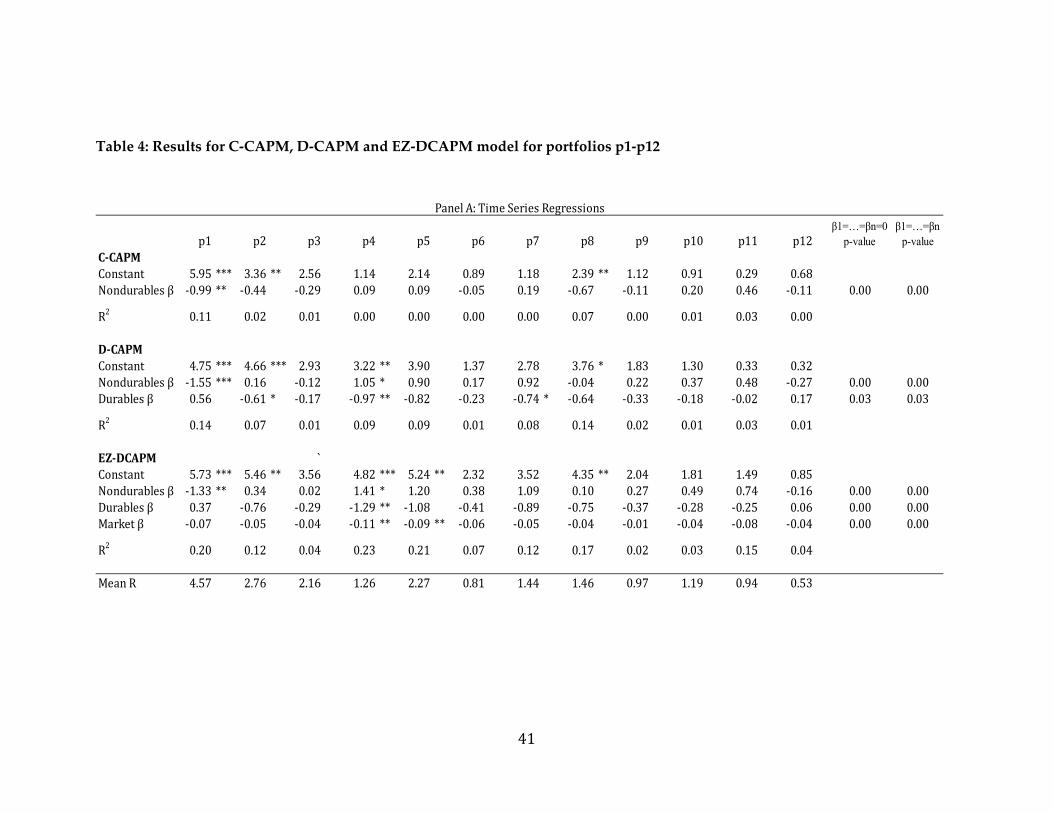
Table 4, Panel A presents the results of the times series regressions. All models, C‐

CAPM, D‐CAPM and EZ‐DCAPM perform poorly. For the C‐CAPM, the beta for portfolio 

p1 is significant at the 5 percent level but has the wrong (negative) sign; none of the other 

betas are significant at  the 5 percent  level. Most of  the betas  for  the D‐CAPM and EZ‐

DCAPM are also  insignificant.   The right‐most columns of Panel A show  that  the beta 

vectors all vary significantly from zero and from each other, permitting identification of 

the prices of risk.  

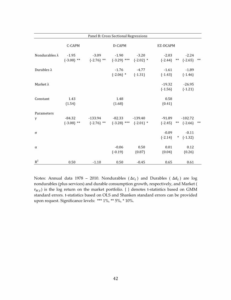
Panel  B  shows  the  results  of  the  cross‐sectional  regressions  for  each  model 

estimated with and without a  constant.    Including  constants  changes  the  fit of  the C‐

CAPM and D‐CAPM models: The constants are not significant at the one‐sided 10 percent 

level and change the R2s from negative to positive levels.  The negative R2s for the models 

that  exclude  the  constants  are  damning:  They  indicate  that  a  simple  constant would 

explain the expected returns better than the model.  

The EZ‐DCAPM model appears to fit better. The constant is not significant and the 

R2 is sizable, at 0.61 and does not change much with the addition of the constant. The price 

12 Equation (21) defines  . 

21

of risk for non‐durable consumption in the EZ‐DCAPM model is statistically significant 

but negative, –2.24 percent.   This negative price of risk  is  implausible, since  the  theory 

predicts that  it should be positive  in the case where the coefficient of risk aversion 

1,and the elasticity of substitution in consumption is less than one  1  . The estimate 

of     in Yogo (2006) for the EZ‐DCAPM is 0.210.  

The coefficient of risk aversion is estimated to be significantly negative in all cases. 

The reason for this can be seen clearly in the case of the C‐CAPM. From equation (5) above 

we know that  

,              (25) 

The Fundamental Theorem of Asset Pricing  implies  that   must be positive 

and so  it  follows  that  if an asset has a positive expected excess return  its returns must 

covary negatively with  the SDF. The SDF  (M),  in  turn,  is marginal utility, which will 

covary negatively with consumption. In the case of the C‐CAPM where the single factor 

is  consumption growth,  this means  that  the model predicts  that  returns  to  the higher 

ranking  dynamic  portfolio  strategies  (those  with  positive  excess  returns)  should  be 

positively correlated with consumption growth. In fact, we find the reverse: the dynamic 

portfolio strategies tend to perform well in states when consumption growth is low, and 

thus provide a hedge against consumption  risk. To be consistent with  the model such 

strategies should earn negative excess returns. 

Figure 2 displays the actual mean excess return to each portfolio ( ) versus the 

predicted  return  ( ′  for  the  cross‐sectional  regressions  that  include  constants. 

Intriguingly, there does appear to be a positive relationship between the predicted and 

22

actual return for all three models, CCAPM, DCAPM and EZ‐DCAPM.  Recall, however, 

that  the  prices  of  risk  are  implausibly  signed,  the  estimates  of  the  coefficient  of  risk 

aversion are negative and the cross‐section regression should exclude the constant. We 

conclude that none of these models can provide a satisfactory explanation for the observed 

returns to the test assets. 

Foreign‐exchange‐based models applied to the returns of portfolios p1 through p12  

Consumption‐based models have generally failed to explain risk adjusted returns 

to many assets, so the results in Table 4 come as no surprise (see Campbell and Cochrane 

(2000)  and  Campbell  (2003)).  This  failure  of  consumption‐based  models  has  led 

researchers  to  look  for  other  risk  factors  that  might  proxy  for  future  investment 

opportunities. In the context of stock returns, it has become commonplace to work with 

factors that are the returns to various stock portfolios (see Fama and French (1993) and 

Carhart  (1997)). We showed  that  these  factors  failed  to explain  the returns  to  technical 

trading rules in foreign exchange markets (Table 3).  

Lustig, Roussanov and Verdelhan (2011) have recently applied this general idea to 

carry  trade  portfolios.  They  form  currency  portfolios  on  the  basis  of  interest  rates. 

Portfolio 1 contains  those currencies with  the  lowest  interest rates; portfolio 6 contains 

those currencies with the highest interest rates. The portfolios are rebalanced at the end 

of each month. From these portfolios Lustig, Roussanov and Verdelhan (2011) construct 

two risk factors. The first factor, which  they denote RX,  is  the average currency excess 

return to going short in the dollar and long in the basket of six foreign currency portfolios. 

The  second  factor, HMLFX,  is  the  return  to  a  strategy  that  borrows  low  interest  rate 

23

currencies (portfolio 1) and invests in high interest rate currencies (portfolio 6), in other 

words a carry trade.13 

Can these factors explain the cross‐sectional variation in expected returns across 

the 12 technical portfolios that were sorted on past Sharpe ratio? We examine this question 

with GMM estimation of beta‐return models using the RX and HMLFX   risk factors that 

enable us to estimate the factor risk premia (  and  ) and the parameters of the 

model. Because  the  factors are  returns  to  tradable portfolios we can  test  the model by 

comparing the estimates of the risk premia with the factor means. We reject the model if 

they differ significantly.   

, , , , , ,          (26) 

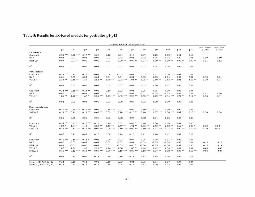
The “LV factors” subsection of panel A of Table 5 shows that the betas on the RX 

factor are small and always insignificant. However, for eight of the dynamic portfolios the 

betas on the HMLFX factor are significantly negative at the ten percent level, or higher, and 

all of  the point estimates are negative  (row 3, Table 5). The negative signs of  the betas 

suggest that the returns to the technical trading rules tend to be high when the carry trade 

returns are  low. The HMLFX   betas  for portfolios p1, p3, p4, and p5 are not significant, 

however, and the alphas for the top five portfolios are often significant and always higher 

than  the  unadjusted  mean  returns.  The  fact  that  the  constants  are  higher  than  the 

unadjusted  mean  returns  indicates  that  accounting  for  HMLFX  and RX  risk  actually 

deepens  the puzzle of  the profitability of  technical  trading rules. These results make  it 

13 RX and HMLFX are very similar to the first two principal components of the returns to the 6 portfolios.  

24

seem unlikely that any risk factor that explained the carry trade could also explain the 

technical returns.  

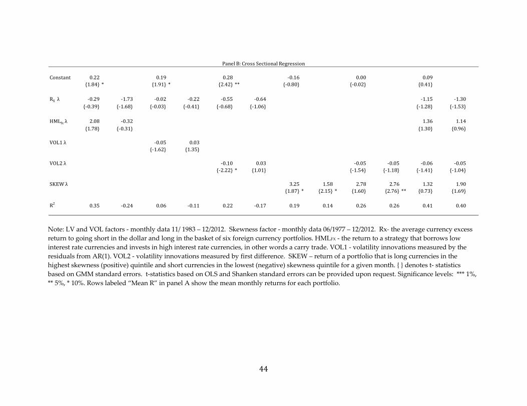
In the second stage of the HMLFX–RX regression, the price of risk for the HMLFX   

factor is 2.08, with a t statistic of 1.78, which is not significant at the 5 percent level for a 

one‐sided test.14 The R2 for this regression with the constant is 0.35 (Table 5, Panel B). But 

the constant in the regression is 0.22, with a t statistic of 1.84, and this is significant at the 

5%  level  for  a  one‐sided  test.  Excluding  the  constant makes  the  R2  negative  (‐0.24), 

implying that the HMLFX   factor does not explain the cross‐section of dynamic portfolio 

returns.  

Volatility is another factor that can potentially explain the returns to investment 

strategies.  Indeed, Menkhoff,  Sarno,  Schmeling  and  Schrimpf  (2012a)  find  that  global 

foreign exchange volatility  is an  important factor  in explaining carry trade returns.   To 

investigate this factor’s explanatory power for our technical returns, we estimate a global 

volatility  factor  in  a manner  very  similar  to  that  of Menkhoff,  Sarno,  Schmeling  and 

Schrimpf (2012a). We first calculate the monthly return variance for each of the available 

exchange rates at each month in our sample and then calculate a global foreign exchange 

volatility factor from the first principal component of the monthly variances. VOL1 is the 

series of innovations of an AR(1) process fit to this principal component while VOL2 is 

the first difference  in this principal component. We then estimate a beta representation 

using these volatility factors and a dollar exposure factor that Menkhoff, Sarno, Schmeling 

14  The  t  statistics  in  the  regression with  a  constant  have  9  degrees  of  freedom  (12  observations  less  3 

coefficients). The  two‐sided 10, 5 and 1 percent critical values  for  this distribution are 1.83, 2.26 and 3.25, 

respectively.  

25

and Schrimpf (2012a) note is very similar to the Lustig, Roussanov and Verdelhan (2011) 

RX factor. Menkhoff, Sarno, Schmeling and Schrimpf (2012a) denote this as the DOL factor 

in their work.  

, , , 1          (27) 

, , , 2           (28) 

Table 5 displays the results from the GMM estimation of the beta system.  Panel A 

of  Table  5  shows  that  the  betas  on  RX  are  not  jointly  statistically  significant  nor 

significantly different from each other (see rows labeled “VOL factors”).  Thus the price 

of RX risk  is not  identified.   In contrast, betas on  the volatility factors are positive and 

highly significant but do not appear to capture any of the cross‐sectional spread in returns. 

That is, there is no obvious pattern to the betas from the low to high ranking portfolios.  

Instead, higher volatility seems to predict higher returns to all technical portfolios, both 

good and bad.  

Panel B of Table 5 shows no evidence for a negative price of volatility risk, as the 

theory  would  predict,  when  one  omits  a  constant  in  the  cross‐sectional  equation.  

Specifically, the prices of risk on VOL1 and VOL2 are positive but insignificant with no 

constant,  and  the  R2s  of  the  second  stage  regressions  are  negative  if  no  constant  is 

permitted (see columns 3 to 6, Panel B).  In addition, the constant terms are significant. In 

other words,  the  volatility  factor  picks  up  time  series  variation  in  returns which  is 

common  to all portfolios, but  the model does not explain  the cross‐sectional spread  in 

returns, or the level of returns for portfolios p1 and p2.  

26

Researchers have also explored skewness as a risk factor for carry trade returns 

(Rafferty (2012)) and the cross‐section of equity returns (Amaya, Christoffersen, Jacobs, 

and Vasquez  (2011)).   To  investigate whether  exposure  to  skewness  can  generate  the 

returns  to  the  technical  trading  rules, we  form  a  skewness  factor,  SKEW,  a  tradable 

portfolio  that  is  long  currencies  in  the  highest  (positive)  skewness  quintile  and  short 

currencies in the lowest (negative) quintile in a given month. We then estimate the model’s 

beta representation and present those results in Table 5.  

, ,              (29) 

The skewness  factor subsection of panel A of Table 5 shows  that  the skewness 

betas are all positive and highly significant. One cannot, however, reject the hypothesis 

that they are all equal to each other, precluding strong identification of the prices of risk.  

Also, the constants in the time series regressions are generally highly significant and very 

close in magnitude to the excess returns to the test assets. Thus, the skewness factor is able 

to account for at most ten percent of the returns to these assets.  

Macro‐based model applied to the returns of portfolios p1 through p12 

Berg and Mark (2015) use results from Backus et al. (2002) to relate expected excess 

carry  trade  returns  to  the  variance  and  skewness  of  SDFs. Holding  currencies  from 

countries whose  log  SDFs  exhibit more  variance  or  positive  skewness  is  “risky”  and 

investors in those currencies receive an excess return. Berg and Mark (2015) test a number 

of  quarterly macro  variables  that  could  be  closely  related  to  the  SDF  as  explanatory 

variables  for  carry  trade portfolio  returns. They  find  that  the  skewness of a  country’s 

unemployment gap is a robust risk factor priced into currency excess returns.   

27

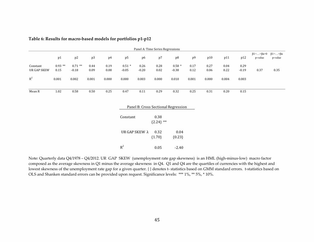
To  determine  whether  this  unemployment  gap  skewness  factor  could  be 

responsible  for  the  returns  to  technical  trading, we  follow  Berg  and Mark  (2015)  in 

constructing such a factor from quarterly macro data, and then we use it as a risk factor 

in a beta representation. Because the macro data are available at a quarterly frequency — 

rather than monthly, as in the previous exercises — we estimate the unemployment gap 

skewness risk factor separately and report the results in Table 6. The functional form of 

the regression is as follows:  

, ,                                                        (30) 

Panel A  of  Table  6  shows  that  none  of  the  betas  on  the  unemployment  gap 

skewness are significantly different from zero. Neither are they jointly different from zero 

or from each other, leaving the risk premium only weakly identified.  Panel B shows that 

the R2  is  small  in  the model with a  constant and negative  in  the model excluding  the 

constant. In summary, there is no evidence that the unemployment skewness gap explains 

the returns to technical trading.  

Liquidity‐based model applied to the returns of portfolios p1 through p12 

Finally, we consider the possibility that a factor for global FX liquidity may explain 

technical  trading  returns. Although  researchers have  actively  investigated  liquidity  in 

bond and equity markets, there has been much less such research in FX markets. Using 

three years of intraday data, Mancini, Ranaldo, and Wrampelmeyer (2013)  showed that 

liquidity  risk  explains  carry  trade  returns;  specifically,  low  interest  currencies  (with 

negative  carry  returns) offer  insurance  against  liquidity  risk. Karnaukh, Ranaldo,  and 

Söderlind (2015) extended this work by establishing that one can accurately measure FX 

28

liquidity with daily data. The authors explore the accuracy of the  liquidity measure by 

examining correlations between several  low  frequency measures and a high  frequency 

measure based on transaction prices.  

Thus,  researchers have not previously  investigated  liquidity as a  risk source of 

technical trading returns. A measure of liquidity, which covers a sufficiently long sample 

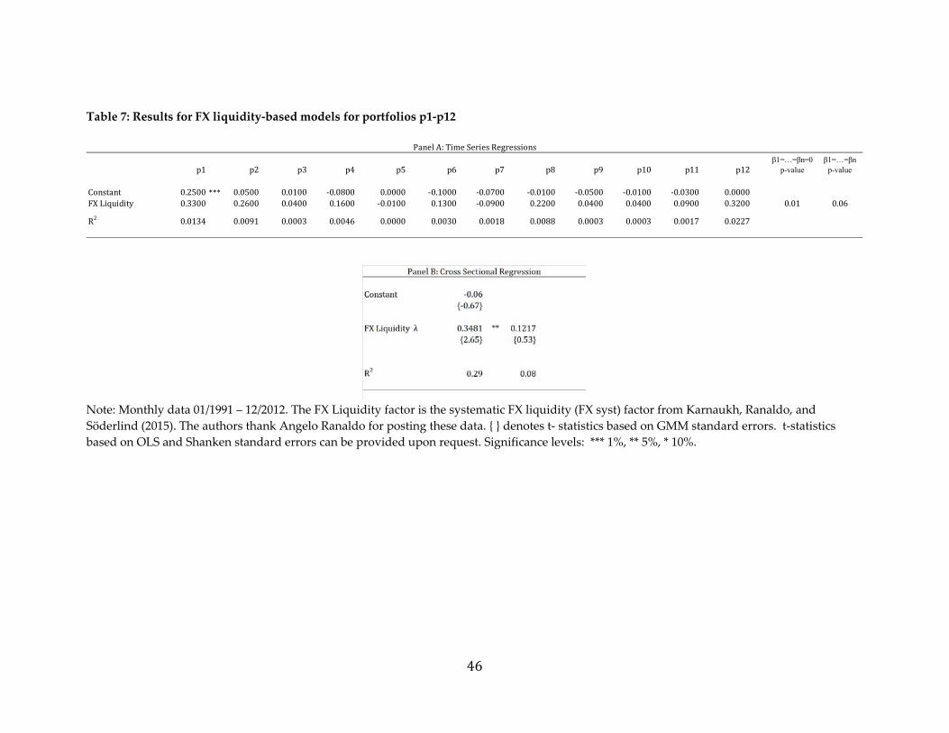
period to make this hypothesis testable, has only recently become available. We use the 

FX  liquidity measure  constructed  by  Karnaukh,  Ranaldo  and  Söderlind  (2015), who 

construct an accurate measure of liquidity with low frequency (daily) data. Their sample 

coincides with our  sample  from  January 1991  to December 2012. We use  the monthly 

liquidity measure  and,  as with previous  factors,  test  the  liquidity  factor  in  the Fama‐

MacBeth two‐stage model.  

, ,                                                             (31) 

Table 7 shows the results of this estimation. None of the coefficients on FX liquidity 

are significant. The price of  liquidity risk  is significant  in  the cross‐sectional regression 

with a constant, but as discussed previously (Burnside (2011)) a substantial difference in 

the price of risk estimate in the regression with and without a constant is an indication of 

poor fit. Therefore, we conclude that FX liquidity has no explanatory power for technical 

trading returns. 

Discussion and Conclusion  

Researchers have long documented the profitability of technical analysis in foreign 

exchange  rates.  Studies  that  found  positive  results  include  Poole  (1967), Dooley  and 

29

Shafer  (1984),  Sweeney  (1986), Levich  and Thomas  (1993), Neely, Weller  and Dittmar 

(1997), Gençay (1999), Lee, Gleason and Mathur (2001) and Martin (2001).  

Despite such a substantial record of documented gains, the reasons for this success 

remain mysterious.  The  findings  of Neely  (2002)  appear  to  rule  out  the  central  bank 

intervention explanation suggested by LeBaron  (1999). To  investigate  the possibility of 

data snooping, data mining and publication bias, Neely, Weller and Ulrich (2009) analyze 

the performance of rules  in  true out‐of‐sample  tests  that occur  long after an  important 

study. They conclude that data snooping, data mining and publication bias are unlikely 

explanations.   

It  remains possible, however,  that  exposure  to  some  sort of  risk generates  the 

technical  trading  rule profitability. Recently,  several  authors have  considered modern 

techniques for risk adjustment of the carry trade or momentum rules in foreign exchange 

markets. If these risk‐based explanations for the carry trade could also explain the returns 

to technical trading in foreign exchange markets, it would appear very likely that these 

factors represent genuine sources of risk. With that  in mind, the goal of this paper has 

been to apply an exhaustive range of risk adjustment techniques to evaluate the evidence 

that exposure to risk plausibly explains the profitability of technical analysis in the foreign 

exchange market. 

We examine many types of risk adjustment models, including the CAPM, a four 

factor model, several consumption‐based models, factors that explain equity returns and 

factors motivated by the carry trade puzzle, including a dollar factor, a carry trade factor, 

foreign exchange volatility,foreign exchange skewnessandtheskewnessofunemployment

30

gaps,andliquidityrisk. We find that no model of risk adjustment can plausibly explain the 

very robust findings of profitability of technical analysis in the foreign exchange market. 

 

 

   

31

References  

 

Allen, Helen, and Mark P. Taylor. (1990). Charts, noise and fundamentals in the London 

foreign exchange market. Economic Journal, 100(400), 49–59. 

Ang, Andrew, Joseph Chen, and Yuhang Xing. (2006). Downside risk. Review of Financial 

Studies, 19(4), 1191 – 1239. 

Amaya, Diego, Peter Christoffersen, Kris Jacobs, and Aurelio Vasquez. (2011). Do realized 

skewness  and  kurtosis  predict  the  cross‐section  of  equity  returns?.  (No.  2011‐44). 

School of Economics and Management, University of Aarhus. 

Backus, David K., Silverio Foresi, and Chris I. Telmer. (2002). Affine term structure models 

and the forward premium anomaly. Journal of Finance, 56(1), 279 – 304. 

Berg, Kimberly A., and Nelson C. Mark.  (2018). Global macro  risks  in currency excess 

returns. Journal of Empirical Finance, 45, 300 – 415.  

Bernard, Arnold. (1984). How to Use the Value Line Investment Survey: A Subscriberʹs 

Guide (Value Line, New York). 

Burnside,  Craig.  (2011).  The  cross  section  of  foreign  currency  risk  premia  and 

consumption growth risk: Comment. American Economic Review, 101(7), 3456 – 3476.  

Burnside, Craig.  (2012). Carry  trades and risk,  in Handbook of Exchange Rates  (eds.  J. 

James, I. Marsh, and L. Sarno), Vol. 2. John Wiley & Sons, Inc. Hoboken, NJ. 

Campbell, John Y. (2003). Consumption‐based asset pricing. Handbook of the Economics 

of Finance, 1(b), 803‐887. 

32

Campbell,  John Y., and  John H. Cochrane.  (2000). Explaining  the poor performance of 

consumption‐based asset pricing models. The Journal of Finance, 55(6), 2863 – 2878. 

Carhart, Mark M.  (1997). On  persistence  in mutual  fund  performance.  The  Journal  of 

Finance, 52(1), 57 – 82.  

Cochrane, John H. (2005). Asset Pricing: (Revised Edition). Princeton University Press. 

Cornell, W. Bradford, and  J. Kimball Dietrich.  (1978). The efficiency of  the market  for 

foreign exchange under floating exchange rates. Review of Economics and Statistics, 6(1), 

111 – 120. 

Dooley, Michael P.,  and  Jeffrey R.  Shafer.  (1976). Analysis  of  short‐run  exchange  rate 

behavior: March 1973 to September 1975. Federal Reserve Board, International Finance 

Discussion Paper, No. 123.  

Dooley, Michael P.,  and  Jeffrey R.  Shafer.  (1984). Analysis  of  short‐run  exchange  rate 

behavior: March  1973  to November  1981,  in David Bigman  and Teizo Taya,  eds.: 

Floating Exchange Rates  and  the State  of World Trade Payments,  (Ballinger Publishing 

Company, Cambridge, MA).  

Fama, Eugene F., and Kenneth R. French. (1993). Common risk factors in the returns on 

stocks and bonds. Journal of Financial Economics, 33(1), 3–56. 

Fama, Eugene F., and James D. MacBeth. (1973). Risk, return and equilibrium: Empirical 

tests. Journal of Political Economy, 81(3), 607–636. 

Fama, Eugene F. (1970). Efficient capital markets: A review of theory and empirical work. 

The Journal of Finance, 25(2), 383 – 417. 

33

Gençay,  Ramazan.  (1999).  Linear,  non‐linear  and  essential  foreign  exchange  rate 

prediction with simple technical trading rules. Journal of International Economics, 47(1), 

91–107.  

Hsu, Po‐Hsuan, Mark P. Taylor,  and Zigan Wang.  (2016). Technical  trading:  Is  it  still 

beating the foreign exchange market?. Journal of International Economics, 102, 188 – 208.  

Jegadeesh, Narasimhan,  and Sheridan Titman.  (1993). Returns  to buying winners  and 

selling losers: Implications for stock market efficiency. The Journal of Finance, 48(1), 65 

– 91. 

Karnaukh,  Nina,  Angelo  Ranaldo,  and  Paul  Söderlind.  (2015).  Understanding  FX 

liquidity. The Review of Financial Studies, 28(11), 3073 – 3108. 

LeBaron,  Blake.  (1999).  Technical  trading  rule  profitability  and  foreign  exchange 

intervention. Journal of International Economics, 49(1), 125–143. 

Lee, Chun I., Kimberly C. Gleason, and Ike Mathur. (2001). Trading rule profits in Latin 

American currency spot rates. International Review of Financial Analysis, 10(2), 135–156.  

Lettau, Martin, Matteo Maggiori, and Michael Weber. (2014). Conditional risk premia in 

currency markets and other asset classes. Journal of Financial Economics, 114(2), 197 – 

225. 

Levich, Richard M., and Lee R. Thomas III. (1993). The significance of technical trading‐

rule  profits  in  the  foreign  exchange  market:  A  bootstrap  approach.  Journal  of 

International Money and Finance, 12(5), 451–474. 

Logue, D. E., and R. J. Sweeney. (1977). ‘White noise’ in imperfect markets: The case of the 

franc/dollar exchange rate. Journal of Finance, 32(3), 761 – 768.  

34

Lustig, Hanno, Nikolai Roussanov, and Adrien Verdelhan. (2011). Common risk factors 

in currency markets.  Review of Financial Studies, 24(11), 3731‐3777. 

Lustig, Hanno, and Adrien Verdelhan. (2007). The cross section of foreign currency risk 

premia and consumption growth risk. American Economic Review, 97(1): 89–117. 

Lustig, Hanno, and Adrien Verdelhan. (2011). The cross section of foreign currency risk 

premia and consumption growth risk: Reply. American Economic Review, 101(7), 3477 

– 3500. 

Mancini,  Loriano,  Angelo  Ranaldo,  and  Jan Wrampelmeyer.  (2013).  Liquidity  in  the 

foreign exchange market: Measurement, commonality, and risk premiums. The Journal 

of Finance, 68(5), 1805 – 1841. 

Martin, Anna D. (2001). Technical trading rules in the spot foreign exchange markets of 

developing countries. Journal of Multinational Financial Management, 11(1), 59 – 68.  

Menkhoff, Lukas, Lucio Sarno, Maik Schmeling, and Andreas Schrimpf.  (2012a). Carry 

trades and global foreign exchange volatility. Journal of Finance, 67(2), 681 – 718. 

Menkhoff,  Lukas,  Lucio  Sarno,  Maik  Schmeling,  and  Andreas  Schrimpf.  (2012b). 

Currency momentum strategies. Journal of Financial Economics, 106(3), 660 – 684. 

Menkhoff, Lukas, and Mark P. Taylor. (2007). The obstinate passion of foreign exchange 

professionals: Technical analysis. Journal of Economic Literature, 45(4), 936 – 972. 

Neely, Christopher J., Paul A. Weller, and Rob Dittmar. (1997). Is Technical analysis in the 

foreign  exchange market  profitable? A  genetic  programming  approach.  Journal  of 

Financial and Quantitative Analysis, 32(4), 405 – 426.  

35

Neely, Christopher J. (2002). The temporal pattern of trading rule returns and exchange 

rate intervention: Intervention does not generate technical trading rule profits. Journal 

of International Economics, 58(1), 211–232. 

Neely, Christopher J., and Paul A. Weller. (2013). Lessons from the evolution of foreign 

exchange trading strategies. Journal of Banking & Finance, 37(10), 3783 – 3798. 

Neely, Christopher J., Paul A. Weller, and Joshua M. Ulrich. (2009). The adaptive markets 

hypothesis:  Evidence  from  the  foreign  exchange  market.  Journal  of  Financial  and 

Quantitative Analysis, 44(2), 467–488. 

Osler, Carol L.,  and  P.H. Kevin Chang.  (1995). Head  and  shoulders: Not  just  a  flaky 

pattern. Federal Reserve Bank of New York Staff Report No. 4. 

Poole, William. (1967). Speculative prices as random walks: An analysis of ten time series 

of flexible exchange rates. Southern Economic Journal, 33(4), 468–478. 

Rafferty, Barry. (2012). Currency Returns, Skewness and Crash Risk. Skewness and Crash 

Risk (March 15, 2012). 

Shanken, Jay. (1992). On the estimation of beta‐pricing models. Review of Financial Studies, 

5(1), 1–33. 

Sweeney, Richard J. (1986). Beating the foreign exchange market. Journal of Finance, 41(1), 

163–182. 

Taylor, Mark P.,  and Helen Allen.  (1992). The use of  technical  analysis  in  the  foreign 

exchange market. Journal of International Money and Finance, 11(3), 304–314. 

36

Taylor, Stephen J. (1994). Trading futures using a channel rule: A study of the predictive 

power of technical analysis with currency examples. Journal of Futures Markets, 14(2), 

215 – 235.  

Yogo, Motohiro.  (2006). A Consumption‐based  explanation  of  expected  stock  returns. 

Journal of Finance, 61(2), 539–580. 

 

 

 

37

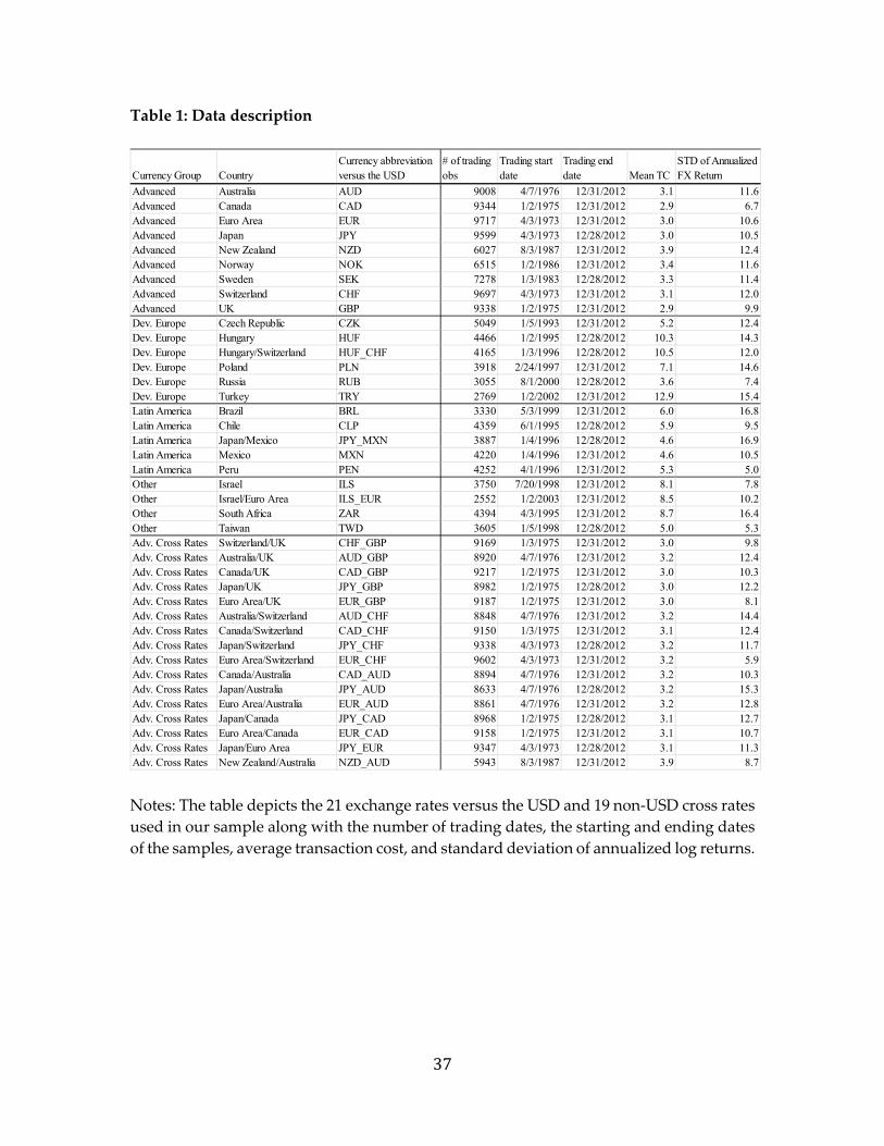
Table 1: Data description  

 

  Notes: The table depicts the 21 exchange rates versus the USD and 19 non‐USD cross rates 

used in our sample along with the number of trading dates, the starting and ending dates 

of the samples, average transaction cost, and standard deviation of annualized log returns. 

Currency Group CountryCurrency abbreviation versus the USD

# of trading obs

Trading start date

Trading end date Mean TC

STD of Annualized FX Return

Advanced Australia AUD 9008 4/7/1976 12/31/2012 3.1 11.6Advanced Canada CAD 9344 1/2/1975 12/31/2012 2.9 6.7Advanced Euro Area EUR 9717 4/3/1973 12/31/2012 3.0 10.6Advanced Japan JPY 9599 4/3/1973 12/28/2012 3.0 10.5Advanced New Zealand NZD 6027 8/3/1987 12/31/2012 3.9 12.4Advanced Norway NOK 6515 1/2/1986 12/31/2012 3.4 11.6Advanced Sweden SEK 7278 1/3/1983 12/28/2012 3.3 11.4Advanced Switzerland CHF 9697 4/3/1973 12/31/2012 3.1 12.0Advanced UK GBP 9338 1/2/1975 12/31/2012 2.9 9.9Dev. Europe Czech Republic CZK 5049 1/5/1993 12/31/2012 5.2 12.4Dev. Europe Hungary HUF 4466 1/2/1995 12/28/2012 10.3 14.3Dev. Europe Hungary/Switzerland HUF_CHF 4165 1/3/1996 12/28/2012 10.5 12.0Dev. Europe Poland PLN 3918 2/24/1997 12/31/2012 7.1 14.6Dev. Europe Russia RUB 3055 8/1/2000 12/28/2012 3.6 7.4Dev. Europe Turkey TRY 2769 1/2/2002 12/31/2012 12.9 15.4Latin America Brazil BRL 3330 5/3/1999 12/31/2012 6.0 16.8Latin America Chile CLP 4359 6/1/1995 12/28/2012 5.9 9.5Latin America Japan/Mexico JPY_MXN 3887 1/4/1996 12/28/2012 4.6 16.9Latin America Mexico MXN 4220 1/4/1996 12/31/2012 4.6 10.5Latin America Peru PEN 4252 4/1/1996 12/31/2012 5.3 5.0Other Israel ILS 3750 7/20/1998 12/31/2012 8.1 7.8Other Israel/Euro Area ILS_EUR 2552 1/2/2003 12/31/2012 8.5 10.2Other South Africa ZAR 4394 4/3/1995 12/31/2012 8.7 16.4Other Taiwan TWD 3605 1/5/1998 12/28/2012 5.0 5.3Adv. Cross Rates Switzerland/UK CHF_GBP 9169 1/3/1975 12/31/2012 3.0 9.8Adv. Cross Rates Australia/UK AUD_GBP 8920 4/7/1976 12/31/2012 3.2 12.4Adv. Cross Rates Canada/UK CAD_GBP 9217 1/2/1975 12/31/2012 3.0 10.3Adv. Cross Rates Japan/UK JPY_GBP 8982 1/2/1975 12/28/2012 3.0 12.2Adv. Cross Rates Euro Area/UK EUR_GBP 9187 1/2/1975 12/31/2012 3.0 8.1Adv. Cross Rates Australia/Switzerland AUD_CHF 8848 4/7/1976 12/31/2012 3.2 14.4Adv. Cross Rates Canada/Switzerland CAD_CHF 9150 1/3/1975 12/31/2012 3.1 12.4Adv. Cross Rates Japan/Switzerland JPY_CHF 9338 4/3/1973 12/28/2012 3.2 11.7Adv. Cross Rates Euro Area/Switzerland EUR_CHF 9602 4/3/1973 12/31/2012 3.2 5.9Adv. Cross Rates Canada/Australia CAD_AUD 8894 4/7/1976 12/31/2012 3.2 10.3Adv. Cross Rates Japan/Australia JPY_AUD 8633 4/7/1976 12/28/2012 3.2 15.3Adv. Cross Rates Euro Area/Australia EUR_AUD 8861 4/7/1976 12/31/2012 3.2 12.8Adv. Cross Rates Japan/Canada JPY_CAD 8968 1/2/1975 12/28/2012 3.1 12.7Adv. Cross Rates Euro Area/Canada EUR_CAD 9158 1/2/1975 12/31/2012 3.1 10.7Adv. Cross Rates Japan/Euro Area JPY_EUR 9347 4/3/1973 12/28/2012 3.1 11.3Adv. Cross Rates New Zealand/Australia NZD_AUD 5943 8/3/1987 12/31/2012 3.9 8.7

38

Table 2:  Calibration  

 

   

 C‐CAPM D‐CAPM EZ‐CCAPM EZ‐DCAPM 

     

stdT[M]/ET[M]  0.93 1.22 0.92 1.22       

varT[M]/ET[M]  0.60 0.61 0.59 0.61       

MAE (in %)  1.32 0.96 1.33 0.96       

R2  ‐1.50 ‐0.13 ‐1.50 ‐0.13        

 Notes: The sample  is 1978–2010 (annual data). The returns are those to portfolios p1 to 

p12, as described in the text. The first two rows report the maximum Sharpe ratio (row 1) 

and the price of risk (row 2). The last two rows report the mean absolute pricing error (in 

percentage points) and the R2. Following Yogo (2006), we fixed sigma (σ) at 0.023 (EZ‐

CCAPM and EZ‐DCAPM), alpha (α) at 0.802 (DCAPM and EZ‐DCAPM), delta (δ) at 0.98, 

and rho (ρ) at 0.700 (DCAPM, EZ‐DCAPM). Gamma (γ) is fixed at 41.16 to minimize the 

mean squared pricing error in the EZ‐DCAPM.  

 

 

39

Table 3: Results for CAPM, Quadratic CAPM, Downside risk CAPM and Carhart model for portfolios p1‐p12  

 

p1 p2 p3 p4 p5 p6 p7 p8 p9 p10 p11 p12CAPMConstant 0.39 *** 0.25 *** 0.21 *** 0.13 * 0.20 *** 0.07 0.14 ** 0.14 ** 0.12 * 0.13 ** 0.11 * 0.08Rmβ ‐0.04 * ‐0.05 ** ‐0.04 * ‐0.04 * ‐0.03 ‐0.05 ** ‐0.05 *** ‐0.04 * ‐0.05 *** ‐0.04 ** ‐0.04 * ‐0.04 **

R2 0.01 0.02 0.01 0.02 0.01 0.02 0.03 0.02 0.03 0.03 0.02 0.03

Quad.CAPMConstant 0.26 *** 0.17 ** 0.12 * 0.05 0.14 ** 0.00 0.09 0.07 0.05 0.09 ‐0.02 ‐0.03Rmβ ‐0.03 ‐0.04 * ‐0.03 ‐0.04 * ‐0.02 ‐0.04 ** ‐0.05 *** ‐0.03 ‐0.05 *** ‐0.04 *** ‐0.03 * ‐0.03 **Rm2β 0.65 *** 0.39 0.46 0.38 0.25 0.35 0.23 0.32 0.33 0.20 0.60 ** 0.52 ***

R2 0.04 0.03 0.03 0.03 0.02 0.04 0.03 0.03 0.04 0.03 0.05 0.06

DownsideriskCAPMConstant 0.27 *** 0.14 ** 0.11 * 0.04 0.13 ** ‐0.04 0.03 0.05 ‐0.01 0.04 0.00 ‐0.03RmDown ‐0.10 *** ‐0.09 *** ‐0.08 ** ‐0.07 * ‐0.05 ‐0.09 ** ‐0.08 ** ‐0.07 ** ‐0.10 *** ‐0.08 ** ‐0.08 * ‐0.09 ***

R2 0.03 0.03 0.03 0.02 0.01 0.04 0.03 0.03 0.04 0.03 0.03 0.05

CarhartConstant 0.41 *** 0.27 *** 0.21 *** 0.13 * 0.17 *** 0.07 0.13 * 0.13 ** 0.11 0.12 ** 0.08 0.08Rmβ ‐0.04 * ‐0.05 ** ‐0.03 ‐0.04 ** ‐0.02 ‐0.04 * ‐0.03 ‐0.03 ‐0.04 ** ‐0.03 ‐0.02 ‐0.03SMBβ ‐0.05 * ‐0.04 * ‐0.04 ‐0.02 ‐0.02 ‐0.03 ‐0.03 * ‐0.03 ‐0.04 * ‐0.04 * ‐0.03 ‐0.05 ***HMLβ ‐0.06 * ‐0.03 ‐0.02 ‐0.02 0.01 ‐0.01 0.01 0.01 0.01 0.01 0.02 0.00UMDβ 0.03 * 0.02 0.02 0.02 0.03 ** 0.02 0.02 0.02 0.02 * 0.03 ** 0.03 ** 0.01

R2 0.04 0.03 0.02 0.02 0.02 0.04 0.03 0.03 0.05 0.04 0.03 0.05

MeanR 0.37 0.23 0.19 0.11 0.18 0.05 0.11 0.12 0.09 0.11 0.09 0.06

0.17 0.150.27 0.70

0.00 0.00

0.03 0.130.49 0.94

0.09 0.77

0.00 0.11

PanelA:TimeSeriesRegressionsβ1=…=βn=0

p-valueβ1=…=βn

p-value

0.18 0.78

 

40

 

 

Rmλ 3.34 ‐3.29 2.99 ‐0.61 3.16 2.27{1.44} {‐2.02} * {1.26} {‐0.33} {1.06} {0.62}

Rm2λ 0.17 0.31{1.31} {3.10} **

Downλ ‐3.94 ‐4.08{‐0.76} {‐0.87}

SMBλ ‐1.64 ‐2.41{‐0.44} {‐0.90}

HMLλ ‐3.76 ‐3.50{‐1.92} * {‐1.70}

UMDλ 4.01 5.37{1.08} {1.60}

Constant 0.28 0.18 0.01 0.09{2.33} ** {1.29} {0.04} {0.35}

R2 0.05 ‐0.16 0.18 0.11 0.19 0.19 0.73 0.72

PanelB:CrossSectionalRegressions

CAPM Quad.CAPM CarhartConditionalCAPM

  

Notes: Monthly data 06/1977 – 12/2012. Factors are the excess return on the U.S. 

stock market  ( ),  the  excess  return  on  the  U.S.  stock market  in  downturn 

( ), the size factor (SMB), the value factor ( ) and the momentum factor 

( ). { } denotes t‐statistics based on GMM standard errors.  t‐statistics based on 

OLS  and  Shanken  standard  errors  can be provided upon  request.  Significance 

levels:  *** 1%, ** 5%, * 10%.  

41

Table 4: Results for C‐CAPM, D‐CAPM and EZ‐DCAPM model for portfolios p1‐p12 

 

 

p1 p2 p3 p4 p5 p6 p7 p8 p9 p10 p11 p12C‐CAPMConstant 5.95 *** 3.36 ** 2.56 1.14 2.14 0.89 1.18 2.39 ** 1.12 0.91 0.29 0.68Nondurablesβ ‐0.99 ** ‐0.44 ‐0.29 0.09 0.09 ‐0.05 0.19 ‐0.67 ‐0.11 0.20 0.46 ‐0.11

R2 0.11 0.02 0.01 0.00 0.00 0.00 0.00 0.07 0.00 0.01 0.03 0.00

D‐CAPMConstant 4.75 *** 4.66 *** 2.93 3.22 ** 3.90 1.37 2.78 3.76 * 1.83 1.30 0.33 0.32Nondurablesβ ‐1.55 *** 0.16 ‐0.12 1.05 * 0.90 0.17 0.92 ‐0.04 0.22 0.37 0.48 ‐0.27Durablesβ 0.56 ‐0.61 * ‐0.17 ‐0.97 ** ‐0.82 ‐0.23 ‐0.74 * ‐0.64 ‐0.33 ‐0.18 ‐0.02 0.17

R2 0.14 0.07 0.01 0.09 0.09 0.01 0.08 0.14 0.02 0.01 0.03 0.01

EZ‐DCAPM `Constant 5.73 *** 5.46 ** 3.56 4.82 *** 5.24 ** 2.32 3.52 4.35 ** 2.04 1.81 1.49 0.85Nondurablesβ ‐1.33 ** 0.34 0.02 1.41 * 1.20 0.38 1.09 0.10 0.27 0.49 0.74 ‐0.16Durablesβ 0.37 ‐0.76 ‐0.29 ‐1.29 ** ‐1.08 ‐0.41 ‐0.89 ‐0.75 ‐0.37 ‐0.28 ‐0.25 0.06Marketβ ‐0.07 ‐0.05 ‐0.04 ‐0.11 ** ‐0.09 ** ‐0.06 ‐0.05 ‐0.04 ‐0.01 ‐0.04 ‐0.08 ‐0.04

R2 0.20 0.12 0.04 0.23 0.21 0.07 0.12 0.17 0.02 0.03 0.15 0.04

MeanR 4.57 2.76 2.16 1.26 2.27 0.81 1.44 1.46 0.97 1.19 0.94 0.53

0.00 0.00

0.00 0.00

0.00 0.00

0.03 0.03

0.00 0.00

β1=…=βn=0 p-value

β1=…=βn p-value

0.00 0.00

PanelA:TimeSeriesRegressions

  

42

 

Nondurablesλ ‐1.95 ‐3.09 ‐1.90 ‐3.20 ‐2.03 ‐2.24{‐3.08} ** {‐2.76} ** {‐3.29} *** {‐2.02} * {‐2.44} ** {‐2.65} **

Durablesλ ‐1.76 ‐4.77 ‐1.61 ‐1.89{‐2.06} * {‐1.31} {‐1.43} {‐1.46}

Marketλ ‐19.32 ‐26.95{‐1.56} {‐1.21}

Constant 1.43 1.48 0.58{1.54} {1.68} {0.41}

Parametersγ ‐84.32 ‐133.94 ‐82.33 ‐139.40 ‐91.89 ‐102.72

{‐3.08} ** {‐2.76} ** {‐3.28} *** {‐2.01} * {‐2.45} ** {‐2.66} **

σ ‐0.09 ‐0.11{‐2.14} * {‐1.32}

α ‐0.06 0.50 0.01 0.12{‐0.19} {0.87} {0.04} {0.26}

R2 0.50 ‐1.10 0.50 ‐0.45 0.65 0.61

PanelB:CrossSectionalRegressions

C‐CAPM D‐CAPM EZ‐DCAPM

 Notes:  Annual  data  1978  –  2010.  Nondurables  ( ∆ )  and  Durables  (  ∆ )  are  log 

nondurables (plus services) and durable consumption growth, respectively, and Market ( 

, )  is  the  log  return  on  the market portfolio.  {  } denotes  t‐statistics  based  on GMM 

standard errors. t‐statistics based on OLS and Shanken standard errors can be provided 

upon request. Significance levels:  *** 1%, ** 5%, * 10%. 

43

Table 5: Results for FX‐based models for portfolios p1‐p12  

 

p1 p2 p3 p4 p5 p6 p7 p8 p9 p10 p11 p12LVfactorsConstant 0.35 *** 0.20 *** 0.17 ** 0.06 0.12 0.04 0.10 0.09 0.12 0.15 * 0.11 0.10Rxβ ‐0.02 ‐0.03 ‐0.04 ‐0.02 ‐0.02 ‐0.02 0.01 ‐0.02 ‐0.06 ‐0.04 ‐0.02 0.01HMLfxβ ‐0.03 ‐0.07 * ‐0.05 ‐0.05 ‐0.03 ‐0.08 ** ‐0.09 ** ‐0.07 * ‐0.09 ** ‐0.10 ** ‐0.09 ** ‐0.09 **

R2 0.00 0.02 0.01 0.01 0.01 0.03 0.04 0.02 0.05 0.06 0.04 0.04

VOLfactorsConstant 0.29 *** 0.12 ** 0.11 * ‐0.01 0.08 ‐0.05 0.01 0.03 0.02 0.04 0.02 0.01Rxβ ‐0.01 ‐0.03 ‐0.03 ‐0.01 ‐0.01 ‐0.01 0.01 ‐0.02 ‐0.05 ‐0.04 ‐0.02 0.01VOL1β 2.33 ** 2.15 ** 1.71 2.51 ** 1.70 ** 2.93 *** 1.94 ** 1.75 * 2.60 ** 2.63 ** 2.01 2.63 **

R2 0.03 0.03 0.02 0.05 0.03 0.07 0.03 0.03 0.06 0.07 0.04 0.06

Constant 0.32 *** 0.15 ** 0.13 ** 0.02 0.10 ‐0.02 0.04 0.05 0.05 0.08 0.05 0.04Rxβ ‐0.01 ‐0.03 ‐0.03 ‐0.01 ‐0.01 ‐0.01 0.02 ‐0.02 ‐0.05 ‐0.03 ‐0.02 0.01VOL2β 1.86 ** 1.92 ** 1.67 * 2.39 *** 1.73 *** 2.83 *** 2.22 *** 1.62 ** 2.72 *** 2.64 *** 1.77 ** 2.17 **

R2 0.02 0.03 0.03 0.05 0.03 0.08 0.05 0.03 0.08 0.09 0.03 0.05

SkewnessfactorConstant 0.35 *** 0.20 *** 0.17 *** 0.09 0.16 *** 0.02 0.09 0.10 * 0.07 0.10 * 0.07 0.03SKEWβ 0.10 *** 0.11 *** 0.10 *** 0.09 *** 0.09 *** 0.10 *** 0.10 *** 0.10 *** 0.07 *** 0.08 *** 0.07 *** 0.10 ***

R2 0.05 0.08 0.06 0.06 0.06 0.08 0.07 0.08 0.04 0.05 0.05 0.09

Constant 0.35 *** 0.21 *** 0.17 *** 0.10 0.16 *** 0.02 0.09 * 0.10 * 0.08 0.10 ** 0.07 0.03VOL2β 1.89 * 1.84 * 1.40 2.25 ** 1.43 ** 2.57 ** 1.91 ** 1.63 ** 2.50 ** 2.53 ** 1.62 * 1.88 * 0.00SKEWβ 0.10 *** 0.11 *** 0.10 *** 0.09 *** 0.08 *** 0.10 *** 0.09 *** 0.10 *** 0.07 *** 0.07 ** 0.07 *** 0.10 *** 0.34

R2 0.07 0.11 0.08 0.10 0.08 0.14 0.10 0.11 0.10 0.12 0.07 0.13

Constant 0.31 *** 0.15 ** 0.12 * 0.02 0.08 ‐0.02 0.07 0.06 0.08 0.11 * 0.08 0.06Rxβ ‐0.02 ‐0.03 ‐0.03 ‐0.01 ‐0.02 ‐0.02 0.01 ‐0.03 ‐0.05 ‐0.04 ‐0.03 0.01 0.21 0.18HMLfxβ 0.00 ‐0.03 ‐0.02 ‐0.01 0.01 ‐0.03 ‐0.06 * ‐0.04 ‐0.05 ‐0.06 * ‐0.07 * ‐0.05 0.10 0.11VOL2β 1.87 * 1.74 1.47 2.23 ** 1.76 *** 2.58 ** 1.85 ** 1.44 * 2.42 ** 2.34 ** 1.42 1.81 0.01 0.03SKEWβ 0.11 *** 0.12 *** 0.10 *** 0.09 *** 0.09 *** 0.10 *** 0.09 *** 0.10 *** 0.07 ** 0.08 ** 0.07 ** 0.10 *** 0.00 0.07

R2 0.08 0.13 0.09 0.11 0.10 0.16 0.14 0.13 0.14 0.16 0.09 0.16

MeanR(11/83‐12/12) 0.32 0.15 0.12 0.02 0.10 ‐0.03 0.04 0.05 0.04 0.07 0.04 0.04MeanR(06/77‐12/12) 0.38 0.23 0.19 0.12 0.18 0.05 0.12 0.13 0.09 0.12 0.09 0.06

0.000.00

0.11 0.12

0.30 0.240.00 0.01

0.32 0.260.00 0.01

0.00 0.34

PanelA:TimeSeriesRegressionsβ1=…=βn=0

p-valueβ1=…=βn

p-value

0.19 0.19

 

44

Constant 0.22 0.19 0.28 ‐0.16 0.00 0.09{1.84} * {1.91} * {2.42} ** {‐0.80} {‐0.02} {0.41}

RXλ ‐0.29 ‐1.73 ‐0.02 ‐0.22 ‐0.55 ‐0.64 ‐1.15 ‐1.30{‐0.39} {‐1.68} {‐0.03} {‐0.41} {‐0.68} {‐1.06} {‐1.28} {‐1.53}

HMLfxλ 2.08 ‐0.32 1.36 1.14{1.78} {‐0.31} {1.30} {0.96}

VOL1λ ‐0.05 0.03{‐1.62} {1.35}

VOL2λ ‐0.10 0.03 ‐0.05 ‐0.05 ‐0.06 ‐0.05{‐2.22} * {1.01} {‐1.54} {‐1.18} {‐1.41} {‐1.04}

SKEWλ 3.25 1.58 2.78 2.76 1.32 1.90{1.87} * {2.15} * {1.60} {2.76} ** {0.73} {1.69}

R2 0.35 ‐0.24 0.06 ‐0.11 0.22 ‐0.17 0.19 0.14 0.26 0.26 0.41 0.40

PanelB:CrossSectionalRegression

  

Note: LV and VOL factors ‐ monthly data 11/ 1983 – 12/2012.  Skewness factor ‐ monthly data 06/1977 – 12/2012.  Rx‐ the average currency excess 

return to going short in the dollar and long in the basket of six foreign currency portfolios. HMLFX ‐ the return to a strategy that borrows low 

interest rate currencies and invests in high interest rate currencies, in other words a carry trade. VOL1 ‐ volatility innovations measured by the 

residuals from AR(1). VOL2 ‐ volatility innovations measured by first difference.  SKEW – return of a portfolio that is long currencies in the 

highest skewness (positive) quintile and short currencies in the lowest (negative) skewness quintile for a given month. { } denotes t‐ statistics 

based on GMM standard errors.  t‐statistics based on OLS and Shanken standard errors can be provided upon request. Significance levels:  *** 1%, 

** 5%, * 10%. Rows labeled “Mean R” in panel A show the mean monthly returns for each portfolio.  

 

 

 

 

45

Table 6: Results for macro‐based models for portfolios p1‐p12  

p1 p2 p3 p4 p5 p6 p7 p8 p9 p10 p11 p12

Constant 0.93 ** 0.71 ** 0.44 0.19 0.51 * 0.26 0.28 0.58 * 0.17 0.27 0.04 0.29URGAPSKEW 0.15 ‐0.18 0.09 0.08 ‐0.05 ‐0.20 0.02 ‐0.38 0.12 0.06 0.22 ‐0.19

R2 0.001 0.002 0.001 0.000 0.000 0.003 0.000 0.010 0.001 0.000 0.004 0.003

MeanR 1.02 0.58 0.50 0.25 0.47 0.11 0.29 0.32 0.25 0.31 0.20 0.15

PanelA:TimeSeriesRegressionsβ1=…=βn=0

p-valueβ1=…=βn

p-value

0.37 0.35

  

 

Constant 0.38{2.24} **

URGAPSKEWλ 0.32 0.04{1.70} {0.23}

R2 0.05 ‐2.40

PanelB:CrossSectionalRegression

  

Note: Quarterly data Q4/1978 – Q4/2012. UR  GAP  SKEW  (unemployment rate gap skewness)  is an HML (high‐minus‐low)  macro factor 

composed as the average skewness in Q1 minus the average skewness  in Q4.  Q1 and Q4 are the quartiles of currencies with the highest and 

lowest skewness of the unemployment rate gap for a given quarter. { } denotes t‐ statistics based on GMM standard errors.  t‐statistics based on 

OLS and Shanken standard errors can be provided upon request. Significance levels:  *** 1%, ** 5%, * 10%.  

 

 

46

Table 7: Results for FX liquidity‐based models for portfolios p1‐p12 

 

 Note: Monthly data 01/1991 – 12/2012. The FX Liquidity factor is the systematic FX liquidity (FX syst) factor from Karnaukh, Ranaldo, and 

Söderlind (2015). The authors thank Angelo Ranaldo for posting these data. { } denotes t‐ statistics based on GMM standard errors.  t‐statistics 

based on OLS and Shanken standard errors can be provided upon request. Significance levels:  *** 1%, ** 5%, * 10%.  

 

p1 p2 p3 p4 p5 p6 p7 p8 p9 p10 p11 p12

Constant 0.2500 *** 0.0500 0.0100 ‐0.0800 0.0000 ‐0.1000 ‐0.0700 ‐0.0100 ‐0.0500 ‐0.0100 ‐0.0300 0.0000FXLiquidity 0.3300 0.2600 0.0400 0.1600 ‐0.0100 0.1300 ‐0.0900 0.2200 0.0400 0.0400 0.0900 0.3200

R2 0.0134 0.0091 0.0003 0.0046 0.0000 0.0030 0.0018 0.0088 0.0003 0.0003 0.0017 0.0227

PanelA:TimeSeriesRegressionsβ1=…=βn=0

p-valueβ1=…=βn

p-value

0.01 0.06

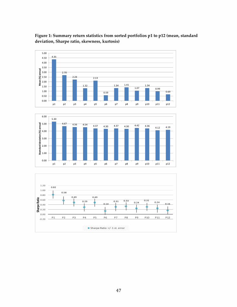
47

Figure 1: Summary return statistics from sorted portfolios p1 to p12 (mean, standard 

deviation, Sharpe ratio, skewness, kurtosis) 

 

  

  

    

4.35

2.70

2.24

1.32

2.13

0.59

1.34 1.411.07

1.340.99

0.69

0.00

0.50

1.00

1.50

2.00

2.50

3.00

3.50

4.00

4.50

5.00

p1 p2 p3 p4 p5 p6 p7 p8 p9 p10 p11 p12

Mean

 (%) annual

5.30

4.67 4.56 4.54 4.37 4.30 4.37 4.30 4.42 4.364.12 4.19

0.00

1.00

2.00

3.00

4.00

5.00

6.00

p1 p2 p3 p4 p5 p6 p7 p8 p9 p10 p11 p12

Stam

dard deviation (%

) annual

0.82 

0.58 

0.49 

0.29 

0.49 

0.14 0.31  0.33 

0.24 0.31 

0.24 0.16 

‐0.20

0.00

0.20

0.40

0.60

0.80

1.00

1.20

P1 P2 P3 P4 P5 P6 P7 P8 P9 P10 P11 P12

Sharpe

 Ratio

Sharpe Ratio +/‐ 1 st. error

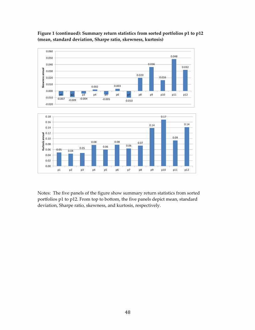
48

Figure 1 (continued): Summary return statistics from sorted portfolios p1 to p12 

(mean, standard deviation, Sharpe ratio, skewness, kurtosis) 

 

Notes:  The five panels of the figure show summary return statistics from sorted 

portfolios p1 to p12. From top to bottom, the five panels depict mean, standard 

deviation, Sharpe ratio, skewness, and kurtosis, respectively. 

‐0.007 ‐0.009 ‐0.004

0.002

‐0.005

0.003

‐0.010

0.020

0.036

0.016

0.048

0.032

‐0.020

‐0.010

0.000

0.010

0.020

0.030

0.040

0.050

0.060

p1 p2 p3 p4 p5 p6 p7 p8 p9 p10 p11 p12

Skewness annual

0.05 0.040.05

0.08

0.06

0.080.06

0.07

0.14

0.17

0.09

0.14

0.00

0.02

0.04

0.06

0.08

0.10

0.12

0.14

0.16

0.18

p1 p2 p3 p4 p5 p6 p7 p8 p9 p10 p11 p12

Kurtosis annual

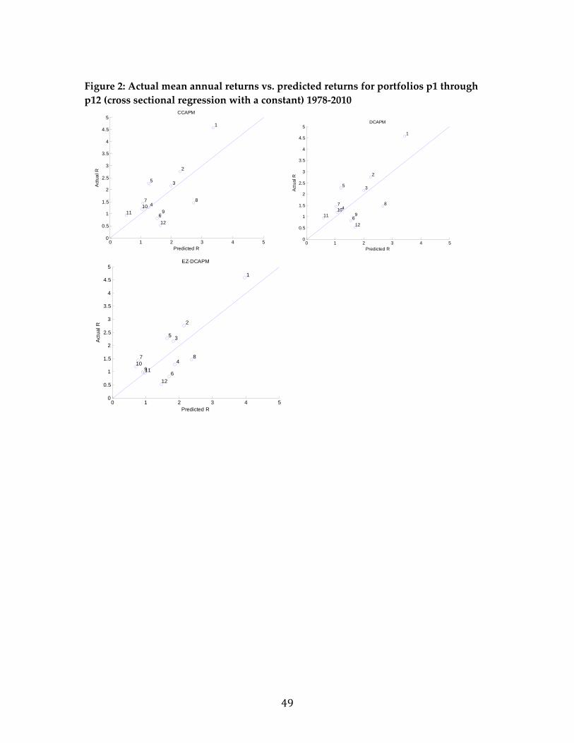
49

Figure 2: Actual mean annual returns vs. predicted returns for portfolios p1 through 

p12 (cross sectional regression with a constant) 1978‐2010 

 

  

0 1 2 3 4 50

0.5

1

1.5

2

2.5

3

3.5

4

4.5

5

1

2

3

4

5

6

7 8

910

11

12

Predicted R

Act

ual R

CCAPM

0 1 2 3 4 50

0.5

1

1.5

2

2.5

3

3.5

4

4.5

5

1

2

3

4

5

6

7 8

910

11

12

Predicted R

Act

ual R

DCAPM

0 1 2 3 4 50

0.5

1

1.5

2

2.5

3

3.5

4

4.5

5

1

2

3

4

5

6

7 8

910

11

12

Predicted R

Act

ua

l R

EZ-DCAPM

Not‐for‐publication appendix 

50

Appendix A – Computation of Transactions Costs 

 

Any study of trading performance must to pay close attention to transaction 

costs, especially when using exotic currencies. The magnitude and the frequency 

of trades influences the impact of transaction costs. Spreads in emerging markets 

are  typically much  larger  than  those  in  developed  countries  and  so  are more 

important  for  emerging  market  currencies.  Burnside  et  al.  (2007)  estimated 

emerging market bid‐ask spreads  to be  two‐to‐four  times bigger  than  those  for 

developed market currencies over the period 1997 to 2006.  

Neely and Weller (2013) used Bloomberg data on one‐month forward bid‐ask 

spreads as the basis for estimating transaction costs that vary both over currencies 

and over  time. Correspondence with several  foreign exchange  traders and with 

the head of the foreign exchange department of a commercial bank led Neely and 

Weller to believe that the quoted Bloomberg spreads substantially overestimated 

the spreads actually available to traders. After comparing spreads from Bloomberg 

with those on traders’ screens and then discussing the size of spreads with traders, 

the  authors  concluded  that  quoted  spreads  were  roughly  three  times  actual 

spreads.  Therefore, Neely  and Weller  calculated  transaction  costs  as  follows: 

Before December 1995, the start of spread data from Bloomberg, the cost of a one‐

way trade for advanced countries (UK, Germany, Switzerland, Australia, Canada, 

Sweden, Norway, New Zealand and Japan) was set at 5 basis points in the 1970s, 

Not‐for‐publication appendix 

51

4 basis points in the 1980s and 3 basis points in the 1990s. The authors set the cost 

at  one  third  of  the  average  of  the  first  500  bid‐ask  observations  for  all  other 

countries.15  Once  Bloomberg  data  become  available,  the  authors  estimated  the 

spread  as  one  third  of  the  quoted  one‐month  forward  spread.  Deliverable 

forwards are available for all countries but Russia, Brazil, Peru, Chile and Taiwan, 

for  which  only  non‐deliverable  forward  data  are  available.  For  cross‐rate 

transaction costs, Neely and Weller use the maximum of the two transaction costs 

against the dollar. All currencies have a minimum of one basis point transaction 

cost at all times. Figure A1 shows the estimated transaction costs for each currency 

over time. The greater magnitude and volatility of these emerging market costs is 

readily apparent. 

The rules/strategies switch between long and short positions in the domestic 

and foreign currencies. The continuously compounded (log) excess return is ztrt+1, 

where zt is an indicator variable taking the value +1 for a long position and –1 for 

a short position, and rt+1 is defined as 

)1ln()1ln(lnln *11 ttttt iiSSr .          (A1) 

15 The costs during the 1970s and 1980s are consistent with triangular arbitrage estimates originally done by 

Frenkel and Levich (1975, 1977) and McCormick (1979), and used by Sweeney (1986) and Levich and Thomas 

(1993). 

Not‐for‐publication appendix 

52

The cumulative excess return from a single round‐trip trade (go long at date t, go 

short at date t + k), with one‐way proportional transaction cost, c , is 

, ∑ ln 1 ln 1 .        (A2) 

A trading strategy may incur transaction costs even when individual trading rules 

do not, and conversely. This will happen if a strategy requires a switch between 

two rules holding different positions but the rules themselves signal no change of 

position. In this case, the strategy incurs a transaction cost but the individual rules 

do not. If, on the other hand, a strategy dictates a switch from a rule requiring—

let us say, a long position at time t to a different rule requiring a long position in 

the same currency at time  1—then no transaction cost is incurred, even though 

one or both individual rules may have signaled a change of position from time t 

to  1. 

   

Not‐for‐publication appendix 

53

References for Appendix A 

Burnside, Craig, Eichenbaum, Martin, and Sergio Rebelo, S. (2007). The returns to 

currency  speculation  in  emerging markets. American  Economic Review, 97(2), 

333‐338. 

Corwin, Shane A., and Paul H. Schultz. (2012). Asimple way to estimate bid‐ask 

spreads from daily high and low prices. Journal of Finance, 67(2), 719–59. 

Frenkel,  Jacob  A.,  and  Richard M.  Levich.  (1975).  Covered  interest  arbitrage: 

Unexploited profits?. Journal of Political Economy, 83(2), 325 – 338.  

Frenkel,  Jacob A., and Richard M. Levich.  (1977). Transaction costs and  interest 

arbitrage: Tranquil versus turbulent periods. Journal of Political Economy, 85(6), 

1209 – 1226. 

Levich, Richard M., and Lee R. Thomas III.  (1993). The significance of  technical 

trading‐rule profits  in  the  foreign  exchange market: A  bootstrap  approach. 

Journal of International Money and Finance, 12(5), 451 – 474. 

McCormick, Frank. (1979). Covered interest arbitrage: Unexploited profits: 

Comment. Journal of Political Economy, 87(2), 411 – 417. 

Neely, Christopher J., and Paul A. Weller. (2013). Lessons from the evolution of foreign 

exchange trading strategies. Journal of Banking & Finance, 37(10), 3783 – 3798. 

Sweeney, Richard J. (1986). Beating the foreign exchange market. Journal of Finance, 

41(1), 163–182. 

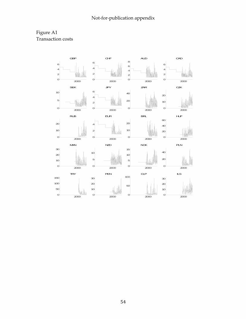
Not‐for‐publication appendix 

54

Figure A1 

Transaction costs  

 

20000

2

4

6

GBP

20000

2

4

6

CHF

20000

2

4

6

8

AUD

20000

2

4

6

CAD

20000

5

10

SEK

20000

2

4

6

JPY

20000

20

40

ZAR

20000

10

20

CZK

20000

10

20

RUB

20000

2

4

EUR

20000

10

20

BRL

20000

20

40

60

HUF

20000

10

20

30

MXN

20000

5

10

NZD

20000

5

10

15

NOK

20000

20

40

PLN

20000

50

100

150

TRY

20000

10

20

30

PEN

20000

50

100CLP

20000

10

20

30

ILS

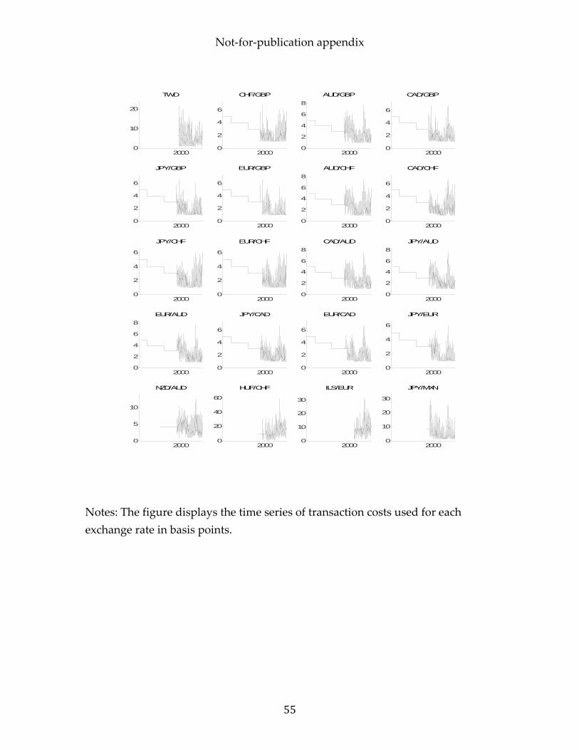
Not‐for‐publication appendix 

55

 

Notes: The figure displays the time series of transaction costs used for each 

exchange rate in basis points.   

 

   

20000

10

20

TWD

20000

2

4

6

CHF/GBP

20000

2

4

6

8

AUD/GBP

20000

2

4

6

CAD/GBP

20000

2

4

6

JPY/GBP

20000

2

4

6

EUR/GBP

20000

2

4

6

8

AUD/CHF

20000

2

4

6

CAD/CHF

20000

2

4

6

JPY/CHF

20000

2

4

6

EUR/CHF

20000

2

4

6

8

CAD/AUD

20000

2

4

6

8

JPY/AUD

20000

2

4

6

8

EUR/AUD

20000

2

4

6

JPY/CAD

20000

2

4

6

EUR/CAD

20000

2

4

6

JPY/EUR

20000

5

10

NZD/AUD

20000

20

40

60

HUF/CHF

20000

10

20

30

ILS/EUR

20000

10

20

30

JPY/MXN

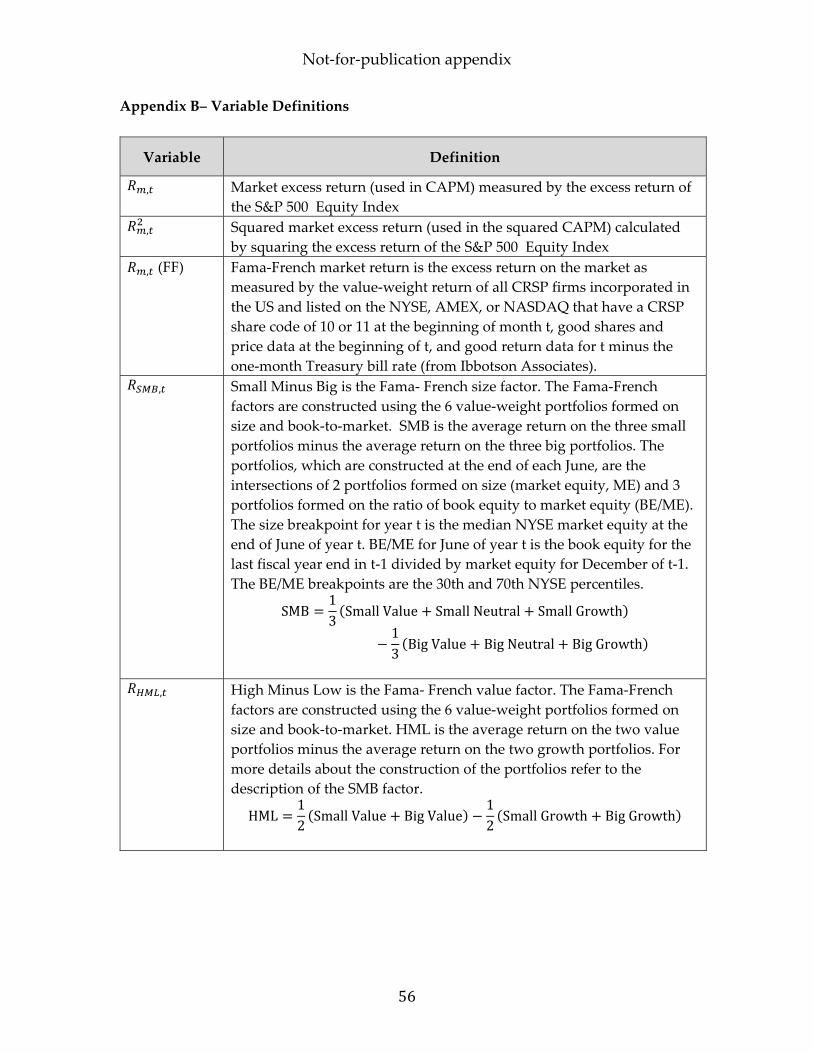
Not‐for‐publication appendix 

56

Appendix B– Variable Definitions 

 

Variable  Definition 

,   Market excess return (used in CAPM) measured by the excess return of 

the S&P 500  Equity Index 

,   Squared market excess return (used in the squared CAPM) calculated 

by squaring the excess return of the S&P 500  Equity Index  

,  (FF)  Fama‐French market return is the excess return on the market as 

measured by the value‐weight return of all CRSP firms incorporated in 

the US and listed on the NYSE, AMEX, or NASDAQ that have a CRSP 

share code of 10 or 11 at the beginning of month t, good shares and 

price data at the beginning of t, and good return data for t minus the 

one‐month Treasury bill rate (from Ibbotson Associates). 

,   Small Minus Big is the Fama‐ French size factor. The Fama‐French 

factors are constructed using the 6 value‐weight portfolios formed on 

size and book‐to‐market.  SMB is the average return on the three small 

portfolios minus the average return on the three big portfolios. The 

portfolios, which are constructed at the end of each June, are the 

intersections of 2 portfolios formed on size (market equity, ME) and 3 

portfolios formed on the ratio of book equity to market equity (BE/ME). 

The size breakpoint for year t is the median NYSE market equity at the 

end of June of year t. BE/ME for June of year t is the book equity for the 

last fiscal year end in t‐1 divided by market equity for December of t‐1. 

The BE/ME breakpoints are the 30th and 70th NYSE percentiles.  

SMB13SmallValue SmallNeutral SmallGrowth

13Big Value Big Neutral BigGrowth  

 

,   High Minus Low is the Fama‐ French value factor. The Fama‐French 

factors are constructed using the 6 value‐weight portfolios formed on 

size and book‐to‐market. HML is the average return on the two value 

portfolios minus the average return on the two growth portfolios. For 

more details about the construction of the portfolios refer to the 

description of the SMB factor.  

HML12Small Value Big Value

12Small Growth BigGrowth  

 

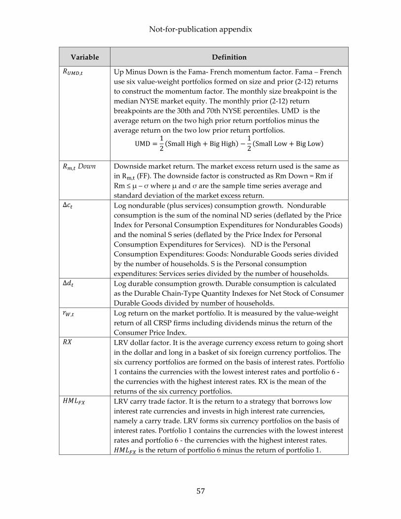
Not‐for‐publication appendix 

57

Variable  Definition 

,   Up Minus Down is the Fama‐ French momentum factor. Fama – French 

use six value‐weight portfolios formed on size and prior (2‐12) returns 

to construct the momentum factor. The monthly size breakpoint is the 

median NYSE market equity. The monthly prior (2‐12) return 

breakpoints are the 30th and 70th NYSE percentiles. UMD  is the 

average return on the two high prior return portfolios minus the 

average return on the two low prior return portfolios.  

UMD12Small High Big High

12Small Low BigLow  

 

,  Down   Downside market return. The market excess return used is the same as 

in R ,  (FF). The downside factor is constructed as Rm Down = Rm if 

Rm ≤ μ – σ where μ and σ are the sample time series average and 

standard deviation of the market excess return.  

∆   Log nondurable (plus services) consumption growth.  Nondurable 

consumption is the sum of the nominal ND series (deflated by the Price 

Index for Personal Consumption Expenditures for Nondurables Goods) 

and the nominal S series (deflated by the Price Index for Personal 

Consumption Expenditures for Services).   ND is the Personal 

Consumption Expenditures: Goods: Nondurable Goods series divided 

by the number of households. S is the Personal consumption 

expenditures: Services series divided by the number of households.  

∆   Log durable consumption growth. Durable consumption is calculated 

as the Durable Chain‐Type Quantity Indexes for Net Stock of Consumer 

Durable Goods divided by number of households.  

,   Log return on the market portfolio. It is measured by the value‐weight 

return of all CRSP firms including dividends minus the return of the 

Consumer Price Index.  

  LRV dollar factor. It is the average currency excess return to going short 

in the dollar and long in a basket of six foreign currency portfolios. The 

six currency portfolios are formed on the basis of interest rates. Portfolio 

1 contains the currencies with the lowest interest rates and portfolio 6 ‐ 

the currencies with the highest interest rates. RX is the mean of the 

returns of the six currency portfolios.  

  LRV carry trade factor. It is the return to a strategy that borrows low 

interest rate currencies and invests in high interest rate currencies, 

namely a carry trade. LRV forms six currency portfolios on the basis of 

interest rates. Portfolio 1 contains the currencies with the lowest interest 

rates and portfolio 6 ‐ the currencies with the highest interest rates. 

 is the return of portfolio 6 minus the return of portfolio 1.  

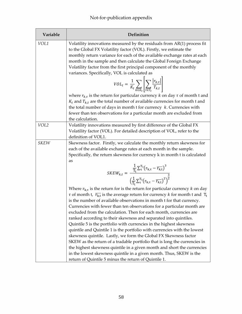
Not‐for‐publication appendix 

58

Variable  Definition 

VOL1  Volatility innovations measured by the residuals from AR(1) process fit 

to the Global FX Volatility factor (VOL). Firstly, we estimate the 

monthly return variance for each of the available exchange rates at each 

month in the sample and then calculate the Global Foreign Exchange 

Volatility factor from the first principal component of the monthly 

variances. Specifically, VOL is calculated as  

1 ,

,∈∈

 

where  ,  is the return for particular currency   on day   of month t and 

 and  ,  are the total number of available currencies for month t and 

the total number of days in month t for currency   . Currencies with 

fewer than ten observations for a particular month are excluded from 

the calculation.  

VOL2  Volatility innovations measured by first difference of the Global FX 

Volatility factor (VOL). For detailed description of VOL, refer to the 

definition of VOL1.  

SKEW 

 

Skewness factor.  Firstly, we calculate the monthly return skewness for 

each of the available exchange rates at each month in the sample.  

Specifically, the return skewness for currency k in month t is calculated 

as 

,

1T ∑ r , r ,

1T ∑ r , r ,

 

Where r ,  is the return for is the return for particular currency   on day 

 of month t,  r ,  is the average return for currency   for month t and  T  is the number of available observations in month t for that currency. 

Currencies with fewer than ten observations for a particular month are 

excluded from the calculation. Then for each month, currencies are 

ranked according to their skewness and separated into quintiles.  

Quintile 5 is the portfolio with currencies in the highest skewness 

quintile and Quintile 1 is the portfolio with currencies with the lowest 

skewness quintile.  Lastly, we form the Global FX Skewness factor 

SKEW as the return of a tradable portfolio that is long the currencies in 

the highest skewness quintile in a given month and short the currencies 

in the lowest skewness quintile in a given month. Thus, SKEW is the 

return of Quintile 5 minus the return of Quintile 1.  

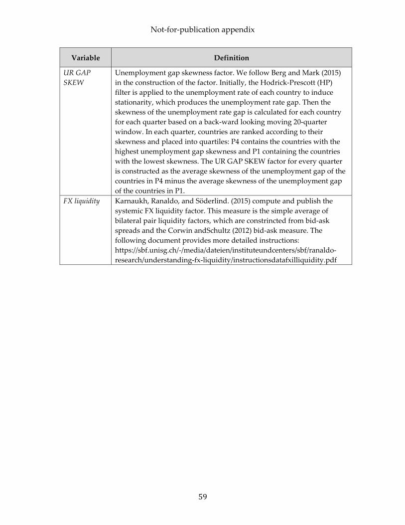
Not‐for‐publication appendix 

59

Variable  Definition 

UR GAP 

SKEW 

 

Unemployment gap skewness factor. We follow Berg and Mark (2015) 

in the construction of the factor. Initially, the Hodrick‐Prescott (HP) 

filter is applied to the unemployment rate of each country to induce 

stationarity, which produces the unemployment rate gap. Then the 

skewness of the unemployment rate gap is calculated for each country 

for each quarter based on a back‐ward looking moving 20‐quarter 

window. In each quarter, countries are ranked according to their 

skewness and placed into quartiles: P4 contains the countries with the 

highest unemployment gap skewness and P1 containing the countries 

with the lowest skewness. The UR GAP SKEW factor for every quarter 

is constructed as the average skewness of the unemployment gap of the 

countries in P4 minus the average skewness of the unemployment gap 

of the countries in P1.  

FX liquidity  

 

Karnaukh, Ranaldo, and Söderlind. (2015) compute and publish the 

systemic FX liquidity factor. This measure is the simple average of 

bilateral pair liquidity factors, which are constrincted from bid‐ask 

spreads and the Corwin andSchultz (2012) bid‐ask measure. The 

following document provides more detailed instructions:  

https://sbf.unisg.ch/‐/media/dateien/instituteundcenters/sbf/ranaldo‐

research/understanding‐fx‐liquidity/instructionsdatafxilliquidity.pdf