Optimal Monetary Policy for the Masses

FEDERAL RESERVE BANK OF ST. LOUISResearch Division

P.O. Box 442St. Louis, MO 63166

RESEARCH DIVISIONWorking Paper Series

James Bullardand

Riccardo DiCecio

Working Paper 2019-009C https://doi.org/10.20955/wp.2019.009

April 2019

The views expressed are those of the individual authors and do not necessarily reflect official positions of the Federal Reserve Bank of St. Louis, theFederal Reserve System, or the Board of Governors.

Federal Reserve Bank of St. Louis Working Papers are preliminary materials circulated to stimulate discussion and critical comment. References inpublications to Federal Reserve Bank of St. Louis Working Papers (other than an acknowledgment that the writer has had access to unpublishedmaterial) should be cleared with the author or authors.

Optimal Monetary Policyfor the Masses∗

James Bullard† Riccardo DiCecio‡

This draft: April 2, 2019

Abstract

We study nominal GDP targeting as optimal monetary policy in a simpleand stylized model with a credit market friction. The macroeconomy we studyhas considerable income inequality, which gives rise to a large private sectorcredit market. There is an important credit market friction because householdsparticipating in the credit market use non-state contingent nominal contracts(NSCNC). We extend previous results in this model by allowing for substan-tial intra-cohort heterogeneity. The heterogeneity is substantial enough thatwe can approach measured Gini coefficients for income, financial wealth, andconsumption in the U.S. data. We show that nominal GDP targeting contin-ues to characterize optimal monetary policy in this setting. Optimal monetarypolicy repairs the distortion caused by the credit market friction and so leavesheterogeneous households supplying their desired amount of labor, a type of“divine coincidence” result. We also further characterize monetary policy interms of nominal interest rate adjustment.Keywords: Optimal monetary policy, life cycle economies, heterogeneous

households, credit market participation, nominal GDP targeting, non-state con-tingent nominal contracting, inequality, Gini coefficients.JEL codes: E4, E5.

∗This paper has benefitted from seminar participant comments during 2018 at the Norges Bank,the Federal Reserve Bank of St. Louis, the Federal Reserve Bank of Dallas, the Texas Monetary Con-ference, the Barcelona Graduate School of Economics Summer Forum–Monetary Policy and Cen-tral Banking, the Expectations and Dynamic Macroeconomic Models conference, the Swiss NationalBank Research Conference and the Fall Midwest Macroeconomics Meetings. We thank Larry Chris-tiano, Davide Debortoli, Harris Dellas, Jordi Galí, Andy Glover, Narayana Kocherlakota, ChristophWinter and Michael Woodford for comments and suggestions. Any views expressed are those of theauthors and do not necessarily reflect the views of others on the Federal Open Market Committee.

†Federal Reserve Bank of St. Louis.‡Federal Reserve Bank of St. Louis. Corresponding author. email: dicecio@stls.frb.org.

1 Income inequality and monetary policy

1.1 Overview

Can monetary policy be conducted in a way that benefits all households in a worldwith substantial heterogeneity? Does monetary policy have an important impact onthe distribution of consumption, income, and financial wealth among heterogeneoushouseholds? The spirit of many modern models of monetary policy is that suchquestions can be pushed into the background via an assumption of a representativehousehold, at least if one is primarily interested in studying only the aggregate impli-cations of monetary policy. However, recent heterogeneous agent models of monetarypolicy surveyed by Galì (2018, p. 102) seem to “... argue that the representativehousehold assumption is less innocuous [than] it may appear.”In this paper we build a simple and stylized model with substantial heterogeneity

in order to help provide some perspective on these questions. We follow recent workby Sheedy (2014), Koenig (2013), Azariadis, Bullard, Singh, and Suda (2018), andBullard and Singh (2019). These papers all provide analyses of economies wherethe household credit market plays a key role and where that market is subject toa friction: non-state contingent nominal contracting (NSCNC). Optimal monetarypolicy is characterized as a version of nominal GDP targeting. The role of monetarypolicy is to provide a type of insurance to private sector credit markets.

1.2 What we do

In this paper, we scale up the natural household heterogeneity ordinarily present inthis model to begin to approach the Gini coefficients in the U.S. data correspondingto the actual degree of income, financial wealth, and consumption inequality. We dothis in a way that maintains the simple and stylized structure of the model so thatthe equilibrium can still be calculated with “pencil and paper” methods, even in thepresence of an aggregate shock and a rich net asset-holding distribution.More specifically, we use a version of the 241-period general equilibrium life-cycle

framework of Bullard and Singh (2019) extended to include heterogeneous life-cycleproductivity. Agents have homothetic preferences defined over consumption andleisure choices and are randomly assigned any one of a continuum of possible pro-ductivity profiles as they enter the economy. This creates substantial intra-cohortheterogeneity in addition to the inter-cohort heterogeneity emphasized in previouspapers. We keep this increased heterogeneity manageable, indexing it to a single pa-rameter, allowing for the complete characterization of optimal monetary policy evenin this case.

1

1.3 Main finding

Our main finding is that nominal GDP targeting continues to characterize the optimalmonetary policy in the economy with the “massive” heterogeneity as we have intro-duced it. The key aspect of policy continues to be countercyclical price level move-ments. The optimal monetary policy repairs the distortion caused by the NSCNCfriction: Despite the substantial heterogeneity, all households benefit from smoothlyoperating credit markets. In the equilibrium we study, households with the samelife-cycle productivity will consume the same amount at each date, a version of thehallmark result in this literature that credit markets under optimal policy are char-acterized by “equity share” contracting.1 Equity share contracting is known to beoptimal when preferences are homothetic.An important aspect of the model equilibrium that makes results particularly

transparent is that the real rate of interest in the economy under optimal monetarypolicy will always be exactly equal to the (stochastic) rate of growth of aggregateoutput. This can be interpreted as the Wicksellian natural rate of interest, and thusan important outcome from the model is that the optimal policy is in this respectvery similar to the optimal policy that would arise in a representative agent NewKeynesian setting.2

With respect to labor supply, the model predicts that under the optimal monetarypolicy, labor supply choices would depend on the stage of the life cycle and thehousehold-specific productivity profile alone and not on the aggregate shock. Thisis a version of the result in Bullard and Singh (2019), suitably adapted to the caseof heterogeneous household productivity profiles. It is a “divine coincidence” resultin that the one friction in the model is completely mitigated through appropriatemonetary policy, and households are therefore able to make their optimal labor supplychoices. Hours worked by various households would be heterogeneous by age butinsensitive to the aggregate shock in this equilibrium.

1.4 Recent related literature

Our paper is most closely related to a relatively recent literature on monetary policywith a NSCNC friction. Koenig (2013), for example, shows that a version of nominalGDP targeting would provide an optimal approach to monetary policy in a two-periodmodel with two households, household credit and a NSCNC friction. Sheedy (2014)provides an extensive discussion of the NSCNC friction and nominal GDP targeting asa mitigant to that friction. Sheedy (2014) also provides a model that includes both aNSCNC friction as well as a sticky price friction. His calibrated economy suggests thatthe NSCNC friction is about nine times more important than the sticky price friction.

1See especially Sheedy (2014) for a discussion.2Koenig (2012) explores the connections between nominal GDP targeting and conventional

Taylor-rule approaches to monetary policy.

2

Bullard (2014) and Werning (2014) provide remarks on Sheedy (2014) and emphasizeideas about how the results may or may not apply to economies with additionalheterogeneity. Azariadis, Bullard, Singh, and Suda (2018) extend the Koenig andSheedy findings to an explicit life-cycle structure3 and focus on issues related to theeffective lower bound on nominal interest rates. They assume inelastic labor supply.Bullard and Singh (2019) study a closely related economy with elastic labor supplyand find that hours worked would be heterogeneous by cohort but independent of theaggregate shock under nominal GDP targeting. The current paper adds substantialintra-cohort heterogeneity to a version of the Bullard and Singh (2019) framework.The literature on monetary policy and heterogeneous households has been expand-

ing in recent years. Galì (2018) summarizes many of the papers that have maintainedNew Keynesian features but added heterogeneous agents in the Aiyagari-Bewley tra-dition. The resulting equilibrium dynamics have been studied by Auclert (2019), Ka-plan, Moll, and Violante (2018), and Bhandari, Evans, Golosov, and Sargent (2018).A broad theme in these papers is that it appears to be problematic to conduct aneasily identifiable monetary policy (such as a Taylor-type monetary policy rule) inthese settings and claim that it is optimal or close to optimal.4 In contrast, in thepresent paper we maintain a high degree of heterogeneity in the sense of equilibriumGini coefficients but limit the form of idiosyncratic risk that households face. Inthis setting we can argue that an easily identifiable monetary policy (nominal GDPtargeting) does have a claim to optimality thanks to the equity share contracting itfacilitates.Our paper represents a departure from some of the heterogeneous agent New

Keynesian literature in two dimensions. First, these papers often have a sticky pricefriction instead of the NSCNC friction studied in this paper. Second, a hallmark ofpapers in much of the heterogeneous agent monetary policy literature is that agentsface uninsurable idiosyncratic labor income risk in every period. We instead includeuninsurable intra-cohort heterogeneity via randomly assigned heterogeneous life-cycleproductivity profiles as agents enter the model. We view these profiles as a stand-in foran exogenous, unmodeled human capital accumulation process, including schooling,parenting, and possibly other types of training that agents may be exposed to priorto entering our analysis.Debortoli and Galì (2018) and Galì (2018) comment on two-agent New Keynesian

models as a parsimonious representation of more complicated forms of heterogeneous

3See also Braun and Oda (2015), Eggertson, Mehrotra, and Robbins (2018), Galì (2014), Sheedy(2018), and Sterk and Tenreyro (2018) for recent studies of monetary policy in life-cycle settings.As Galì (2018) stresses, in these models the real interest rate may be importantly influenced bymonetary policy in ways that are difficult to replicate in representative agent settings.

4Werning (2014) studies cases where incomplete-markets settings do have a clear correspon-dence with representative agent settings. McKay, Nakamura, and Steinsson (2016) study relativelystandard “forward guidance” classes of monetary policy and find attenuated effects relative to therepresentative agent alternative.

3

agent economies with monetary policy.5 The current paper may be viewed as some-what intermediate between models in the Aiyagari-Bewley tradition and two-agentheterogeneous agent models: less complicated than the former, but richer than thelatter.Huggett, Ventura, and Yaron (2011) study the relative effects of the level of human

capital households bring into the life-cycle model at the time they begin to makeeconomic decisions (age 23 in their paper), along with their initial wealth, versustheir ability to learn and the idiosyncratic labor income risk they experience duringtheir lifetimes. The authors argue that most of the action is in the initial conditionsas opposed to the shocks.6 This finding helps motivate our decision to randomlyassign life-cycle productivity profiles to households as they enter the model, ratherthan keeping track of a stochastic household productivity sequence as in Aiyagari(1994) and subsequent research. There is uninsurable labor income risk, but all ofthis risk is borne at the outset of the life cycle for each cohort. This decision affordsus considerable tractability, allowing calculation of “paper and pencil” solutions tothe model even in the face of an aggregate shock.In the present paper there is a single asset that is traded in nominal terms.7

While the model is quite abstract and there is no explicit housing sector, it is perhapsnatural to think of this single asset as a “mortgage-backed security,” because the assetis privately issued by relatively young households to move consumption earlier in thelife cycle than would otherwise be possible; this consumption could be interpretedbroadly as housing services. Households nearer the midpoint of the life cycle wish toown these securities as a way of saving for retirement.There is a large literature on the macroeconomic implications of mortgage markets

following the global financial crisis of 2007-2009. One of the many issues in thisliterature is whether fixed- or variable-rate mortgages change the nature of monetarypolicy transmission. For example, Garriga, Kydland, and Šustek (2017) study howthe monetary transmission mechanism is altered depending on nominal contractingfeatures in mortgage markets and find quantitatively significant impacts dependingon the nature of the shock. Sheedy (2014) emphasizes that fixed- versus variable-rate mortgages would be a quantitatively important consideration in a model with aNSCNC friction. The present paper restricts attention to one-period debt contracting(each period a new contract is signed, which is effective until the following period),and so may be viewed in the spirit of variable-rate mortgages. The issue of fixedrates over longer spans of time would be an additional friction that may be an areaof fruitful study in more quantitatively oriented exercises than the one in this paper.

5See also Ko (2015) for an alternative way to think about how the income and wealth distributionmay impinge on standard New Keynesian dynamics.

6Huggett, Ventura, and Yaron (2011, p. 2924) state, “We find that initial conditions (i.e., in-dividual differences existing at age 23) are more important than are shocks received over the restof the working lifetime as a source of variation in realized lifetime earnings, lifetime wealth, andlifetime utility.”

7For a version with money demand included, see Azariadis, Bullard, Singh, and Suda (2018).

4

This paper is about optimal monetary policy, one that has probably not beenfollowed by actual policymakers during the postwar era. We interpret Doepke andSchneider (2006) as documenting the costly nominal redistribution that may haveoccurred in the U.S. economy as a result. They suggest that so many assets are heldand traded in nominal terms that the welfare consequences of a shock to inflation canbe quantitatively large.We abstract from issues related to the effective lower bound on nominal interest

rates in this version of the model and refer interested readers to Azariadis, Bullard,Singh, and Suda (2018).

2 Environment

2.1 Background on symmetry

We impose an important set of symmetry assumptions on the model. These assump-tions help to control the heterogeneity and keep the model simple and stylized. Thecore result of the symmetry assumptions is that we are able to guess and verify thatthe general equilibrium real rate of interest will be equal to the real rate of growth ofthe economy, even with an aggregate shock and many heterogeneous households.8

Why is symmetry important? In the overlapping generations framework, muchdepends on the relative productivity of the older cohorts versus younger cohortsand by extension on the relative demand for assets versus the relative supply ofthose assets. By keeping these forces in balance, we can understand the baselineequilibrium of the model as a first-best allocation of resources, and thus we will beable to illustrate how monetary policy might overcome the NSCNC friction in orderto attain that allocation. It is of course also interesting to understand how departuresfrom the symmetry assumptions will affect the general equilibrium, presumably usingquantitative methods, and we leave this to future research as it is beyond the scopeof the current paper.Accordingly, we assume the following:

(1) cohorts are of equal size and total population is constant;

(2) the discount factor for all households is unity;

(3) all households have log preferences as defined below;

(4) households’ life-cycle productivity profiles are hump-shaped and symmetric asdefined below.

One of our goals is to keep the analysis simple and stylized in order to be able tounderstand the equilibrium clearly. Accordingly, we have no capital in this version of

8We use the terms “household” and “agent” interchangably in this paper.

5

the model. All loans are repaid according to contractual obligations, and so there isno default in this version. Prices are flexible. Also, we have no borrowing constraintsin this version of the model. Of these, we think capital could be added withoutmaterially affecting the key results. However, default, sticky prices, and borrowingconstraints would change the nature of the equilibrium and thus the characterizationof optimal monetary policy, unless other policy tools were also included to addressthese additional frictions.We now describe the model environment.

2.2 Cohorts

Time is discrete. At each date, a cohort enters the model consisting of a continuumof households indexed i ∈ (0, 1) . Each household in this cohort will make economicdecisions for (T + 1) = 241 consecutive periods and then exit the model in such a waythat the total population remains constant. We interpret this value of T to representa quarterly model in which economic decisions are being made every 90 days. Allinterest rates and growth rates are therefore interpretable in quarterly terms.9 To fixideas, we think of each cohort as one million individuals or more, which is the typeof scale that would be appropriate for a large economy similar to the size of the U.S.or the euro area. We approximate this sort of scale with a continuum of householdsin each cohort, and while we solve all individual household problems, we sometimescharacterize behavior at the cohort level as opposed to the individual level.The model has both real and nominal quantities. We express nearly all variables

in real terms, notably real consumption c and the real wage w. The exception is netasset holding a, which is expressed in nominal terms.Each household i ∈ (0, 1) entering the economy at date t has preferences

Ut,i =

T∑

s=0

η ln ct,i (t+ s) + (1− η) ln `t,i (t+ s) , (1)

where η ∈ (0, 1) controls the relative desirability of real consumption in the consumption-leisure bundle. We use subscripts to denote the date of entry into the model andparentheses to denote real time, so that ct,i (t+ s) represents the date t + s con-sumption of a household i who entered the economy at date t and `t,i (t+ s) ∈ (0, 1)represents the date t + s leisure choice of a household i that entered the economyat date t. Preferences for the households entering the economy at date t − 1 can bedefined analogously in a time-consistent manner as

Ut−1,i =

T−1∑

s=0

η ln ct−1,i (t+ s) + (1− η) ln `t−1,i (t+ s) (2)

9We stress that results are invariant for any integer value of T ≥ 2 and that the choice of Tsimply reflects the time frame for economic decision making. Results also hold in continuous time,i.e., for T →∞.

6

0 60 120 180 240

Quarters

0

1

2

3

4

Figure 1: Baseline endowment profile.

and similarly for all households entering the economy at earlier dates.

2.3 Life-cycle productivity endowments

Each household i ∈ (0, 1) entering the economy at each date t is endowed with a knownsequence of productivity (efficiency) units, “the life-cycle productivity endowment,”denoted by ei = {es,i}

T

s=0 . This notation means that each household i ∈ (0, 1) enteringthe economy has productivity endowment e0,i in the first period of activity, e1,i in thesecond, and so on up to eT,i. Households can sell the productivity units they areendowed with each period on a labor market at an economy-wide competitive realwage per effective efficiency unit and thus earn labor income at each date. We assumethe entire endowment sequence is strictly positive for all households i.As a critical aspect of the symmetry of the model economy, we assume that this

productivity endowment sequence is hump-shaped and symmetric for each householdi. This means that the sequence is monotonically increasing up to the middle-periodendowment, e120,i; that the sequence is hump-shaped in the sense that the middle-period endowment, e120,i, is larger than all other endowments received by household i;that the sequence is monotonically increasing before and decreasing after the middle-period endowment; and that the sequence is symmetric defined as e0,i = eT,i, e1,i =eT−1,i, e2,i = eT−2,i, ....

7

We begin with the following baseline profile:

es = f (s) = 2 + exp

[

−

(s− 120

60

)4]

. (3)

This is a stylized endowment profile that emphasizes that productivity near the be-ginning and end of the life cycle is relatively low, while productivity in the middle ofthe life cycle is relatively high. In short, households will have “peak earning years” forlabor income. It will also turn out that households will choose to work more hoursduring the middle of the life cycle, and so peak labor income will be considerablyhigher than what is suggested by the productivity profile alone. While productivityis low at the beginning and end of the life cycle, we have chosen this profile such thathouseholds will not be tempted to supply zero labor in those circumstances (they maychoose to work very few hours, but they will not choose zero hours). This means thatwe can restrict attention to interior solutions for the equilibria we study, even for anarbitrarily large degree of intra-cohort heterogeneity as defined in the next paragraph.The baseline endowment profile is displayed in Figure 1.10

We now introduce heterogeneity in the life-cycle productivity endowments. Letξ ≥ 1 be a within-cohort dispersion parameter. Each household i ∈ (0, 1) enteringthe economy at date t draws a scaling factor x ∼ U

[ξ−1, ξ

]that yields an endowment

profile es,i = x · es. Thus some households will have a relative abundance of life-cycle productivity, while other households will have a relative dearth of life-cycleproductivity, but all households will face the same pattern of life-cycle productivity.If ξ = 1, there is no dispersion and all households are endowed with the baselineprofile. Because households will never be tempted to supply zero labor no matterwhat scale they are on, we can choose ξ to be arbitrarily large without disturbingthe equilibrium properties we describe below. However, we will show that each of theGini coefficients of the model tends toward a limiting value as ξ increases. We willalso consider an alternative model in which we draw x from a lognormal distributioninstead of a uniform distribution and report results for that case below.We motivate this productivity profile assignment as a stand-in for the end result

of an unmodeled human capital development process–schooling combined with par-enting and perhaps other training–that endowed the incoming agent with the givenlife-cycle productivity, as mentioned in the literature review section above.The set or “mass” of heterogeneous endowment profiles is portrayed by the shaded

area in Figure 2.

10We do not make any claims about this particular profile except that it is simple and convenientfor the issues we discuss in this paper. A wide variety of profiles would satisfy the symmetry criteriaand we could also consider heterogeneity among these various types of profiles. A productivity levelin the middle of the life cycle that is 50 percent higher than that at the beginning or a the end oflife cycle is of the same order of magnitude as much of the quantitative life-cycle literature.

8

Figure 2: Endowment distribution by cohort (shaded area) and a representative en-

dowment profile (line): es,i ∼ es · U(ξ−1, ξ

), es = 2 + exp

[(− s−120

60

)4], ξ = 6.5.

2.4 Assets and the credit market friction

There is a single asset in the model economy, which is privately issued debt. Thisdebt is a credible promise to pay a stated nominal amount in full plus agreed nominalinterest, and is issued by relatively young households who wish to pull consumptionforward in the life cycle. The lenders are households in their peak earning years nearthe middle of the life cycle who wish to accumulate assets for retirement. Giventhis structure, we think it is natural to motivate this abstract asset as representingmortgage-backed securities. The consumption that relatively young households wishto pull forward in the life cycle can be thought of as housing services. Thus, whilethe model is simple and abstract, we think it can be thought of as representing themechanics of a quite large and important private sector credit market. The mortgagedebt outstanding in the U.S. in 2017 was near $15 trillion, which is a ratio to annualGDP of about 0.80.Households borrow in nominal terms and promise to pay off in nominal terms in

a manner that does not depend on the state of the economy:

Definition 1 Non-state contingent nominal contracting: All loan contracts are for

one period, are not state contingent, and are expressed in nominal terms.

Implicitly, there is a second asset in the model, which is currency supplied by the

9

monetary authority. However, in this version of the model we abstract from moneydemand issues altogether and simply assume that the monetary policymaker controlsthe price level P (t) directly. In the last section of the paper, we interpret the directprice level control in terms of direct control over short-term nominal interest rates. Inthis sense, we are making assumptions very similar to the “cashless limit” assumptionin the New Keynesian literature, in which the monetary authority’s control over ashort-term nominal interest rate is simply asserted.11

There is no publicly-issued debt in this version of the model, nor is there any fiscalpolicy of any kind–all government expenditures and taxes are set to zero.We assume that households that are entering the economy at date t hold no net

nominal assets, which we refer to simply as “net assets.” Households that entered intothe economy in previous periods will generally have a non-zero net asset position atdate t, which we denote by at−s,i (t) for s = 1, ..., T and i ∈ (0, 1), which indicates thenet asset holdings carried into the current period from date t− 1 by each member ofeach cohort that entered the economy at the various dates t− s. There will thereforebe a net asset distribution in the economy that we will have to track as part of theequilibrium. However, because all net asset positions will be linear in the real wage,it will be easy to track this distribution.

2.5 Technology

The technology is a simple extension of the endowment economy idea that “one unitof labor produces one unit of the good,” but with appropriate adjustments for life-cycle productivity endowments es,i and labor supply 1−`t−s,i (t) .We denote the levelof aggregate total factor productivity as Q (t) , which we also call, equivalently, thelevel of technology or the level of labor productivity. The gross growth rate of Qfollows a stochastic process. We say

Q (t) = λ (t− 1, t)Q (t− 1) , (4)

where λ (t− 1, t) is the growth rate of productivity between date t − 1 and date t.The stochastic process driving the growth rate of productivity is AR (1) with meanλ:

λ (t, t+ 1) = (1− ρ) λ+ ρλ (t− 1, t) + σε (t+ 1) , (5)

where λ > 1 is the mean growth rate, ρ ∈ (0, 1) denotes the degree of serial correlation,σ > 0 is a scale factor, and ε (t) is a truncated normal random variable with meanzero and bounds ±b, with b > 0, chosen such that the zero lower bound is notencountered12 and the level of technology Q (or other variables like the price level P )

11See, for instance, Woodford (2003) for a discussion of the cashless limit.12The zero lower bound or effective lower bound would be encountered with a sufficiently negative

shock combined with enough serial correlation to cause the expected rate of nominal GDP growthto be negative. See Azariadis, Bullard, Singh, and Suda (2018) for a discussion of this issue.

10

will never be negative.13

Aggregate output is given by

Y (t) = Q (t)L (t) . (6)

If we denote by [1− `t−s,i (t)] ∈ (0, 1) the fraction of time spent working by householdi of cohort t− s , the labor input at date t is given by

L (t) =

∫ 1

0

{e0,i [1− `t,i (t)] + e1,i [1− `t−1,i (t)] + · · ·+ eT,i [1− `t−T,i (t)]} di. (7)

The marginal product of labor is the real wage per effective efficiency unit, given by

w (t) = Q (t) , (8)

and we conclude thatw (t) = λ (t− 1, t)w (t− 1) . (9)

The aggregate real output growth rate is then

Y (t)

Y (t− 1)=

Q (t)L (t)

Q (t− 1)L (t− 1)= λ (t− 1, t)

L (t)

L (t− 1). (10)

A baseline result in this model is that under the optimal monetary policy the equi-librium leisure choices ` are independent of the aggregate shock and hence of thereal wage, so that L (t) is constant in this formula. In particular, various cohortswill make the same leisure choice at the same stage of the life cycle, represented by`t (t) = `t−1 (t− 1), `t−1 (t) = `t−2 (t− 1) , and so on. We therefore conclude that

Y (t) = λ (t− 1, t)Y (t− 1) (11)

in the equilibrium under optimal monetary policy. Along the nonstochastic balancedgrowth path, the gross output growth rate would be λ, the mean rate of productivitygrowth. We will show below that the real interest rate equals the real output growthrate period by period in the stochastic equilibria we study.

2.6 Timing protocol

A timing protocol determines the role of information in the credit sector. We assumethat nature moves first and chooses a continuum of draws defining the heterogeneousproductivity profiles for the entering cohort and a value for ε (t), which implies avalue for the productivity growth rate λ (t− 1, t) and hence a value for today’s realwage w (t). The monetary policymaker moves next and chooses a value for the pricelevel P (t), as described below. Households then take w (t) and P (t) as known andmake decisions to consume and save via non-state contingent nominal contracts forthe following period. These contracts carry a gross nominal interest rate denoted byRn (t, t+ 1). We now turn to defining these contracted values.

13This is just one of many possible stochastic processes that could be used.

11

2.7 Nominal interest rate contracts

All households meet in a competitive market for nominal loans. Households contractby fixing the nominal interest rate on consumption loans one period in advance. Fromthe cohort t household Euler equation, the non-state contingent gross nominal interestrate in effect from period t to period t+ 1, denoted Rn (t, t+ 1), is given by14

Rn (t, t+ 1)−1 = Et

[ct,i (t)

ct,i (t+ 1)

P (t)

P (t+ 1)

]. (12)

We call this the contracted gross nominal interest rate, or simply the “contract rate.”The Et operator indicates that households must use information available as of theend of period t and before the realization of ε (t+ 1). This expression is the same forall households i ∈ (0, 1) in the equilibria we study. In particular, the equity sharefeature of the equilibrium means that all cohorts have the same expectation of theirpersonal consumption growth rates, so that (12) suffices to determine the contractrate. Another way to say this is that there are heterogeneous households in thiseconomy, and in particular some were born at, for instance, date t− 1. These cohortt− 1 households would want to contract at the nominal rate given by

Rn (t, t+ 1)−1 = Et

[ct−1,i (t)

ct−1,i (t+ 1)

P (t)

P (t+ 1)

]. (13)

This would similarly be true for all other households entering the economy at earlierdates up to date t− T (and across all i). However, in the equilibria we study, it willturn out that

ct,i (t)

ct,i (t+ 1)=

ct−1,i (t)

ct−1,i (t+ 1)= · · · =

ct−T,i (t)

ct−T,i (t+ 1), (14)

∀i, so that these expectations will all be the same and hence (12) suffices to determinethe contract rate.Given these considerations, individual expected consumption growth rates are

equal to the expected aggregate nominal consumption growth rate and hence to theexpected rate of nominal GDP growth in the equilibrium we study. This will play animportant role in understanding how monetary policy works in this economy.

2.8 The monetary authority

From the discussion of assets in the subsection above, we have the assumption that themonetary authority controls P (t) directly. We assume that the monetary policymakerhas been asked by an enabling body exogenous to this model to achieve a grossinflation rate of π∗ on average. We now assume that the monetary policymaker uses

14See Chari and Kehoe (1999) for more details.

12

the ability to set the price level at each date t to establish a fully credible policy rule∀t given by

P (t+ 1) =Rn (t, t+ 1)

λr (t, t+ 1)P (t) . (15)

The term Rn (t, t+ 1) is the contract nominal interest rate effective between date tand date t+1, which is the expected rate of nominal GDP growth as described above.The term λr (t, t+ 1) is the realized rate of productivity growth between date t anddate t+1, that is, the realization of the growth rate for λ observed by the policymakerat date t+1. This rule delivers the exogenously given inflation rate of π∗ on average.Because the realized value of productivity growth appears in the denominator, thisrule calls for countercyclical price level movements. This is a hallmark of nominalGDP targeting as discussed in Koenig (2013) and Sheedy (2014).

2.9 Household budget constraints

Households have a simple sequence of budget constraints given the structure of themodel and the fact that net assets are expressed in nominal terms. These budgetconstraints can be aggregated into a consolidated lifetime budget, which is standard.For the cohort entering the economy at date t, household i faces

ct (t) +

T∑

s=1

(P (t+ s)

P (t)

ct,i (t+ s)

Rn (t, t+ s)

)≤

e0w (t) [1− `t,i (t+ s)] +

T∑

s=1

(P (t+ s)

P (t)

es,iw (t+ s) (1− `t,i (t+ s))

Rn (t, t+ s)

), (16)

where

Rn (t, t+ s)=s∏

j=1

Rn (t+ j − 1, t+ j) . (17)

Households entering the economy at earlier dates have a similar constraint over theirremaining lifetime but also have a net asset position that they carry into date t,denoted by at−1,i (t), at−2,i (t) ,. . . , at−T,i (t).Now let us consider just one term in this budget constraint (16), the one applicable

to date t+ 1 given by

· · ·P (t+ 1)

P (t)

ct,i (t+ 1)

Rn (t, t+ 1)· · · ≤ · · ·

P (t+ 1)

P (t)

e1 [1− `t,i (t+ 1)]w (t+ 1)

Rn (t, t+ 1)· · · . (18)

The uncertainty in this expression is coming from the future real wage w (t+ 1),which is stochastic. We can substitute the policy rule (15) directly into this ex-pression. Noting that w (t+ 1) = λ (t, t+ 1)w (t) and that ` choices will depend oncontemporaneous consumption choices alone, the stochastic element, λ (t, t+ 1), will

13

cancel on the right-hand side and thus future income will become deterministic fromthe perspective of the household. This cancellation occurs for all other terms on theright-hand side of this expression, as well as for all other similar expressions for allother agents in the economy. The policymaker is providing a form of insurance tohouseholds.More detail on the model solution is provided below and in the Appendix.

2.10 The model’s simple solution

The details of the model solution are given in the Appendix, but we provide a heuristicdiscussion here.We are interested in focusing on a stationary equilibrium in which time extends

from the infinite past to the infinite future and where the monetary policy rule isfollowed credibly for all time. To obtain the solution, we begin with the problem ofa single household i entering the economy at an arbitrary date t. This household hasthe preferences given above and faces a lifetime budget constraint expressed in nomi-nal net asset terms. We can substitute the policymaker rule into this lifetime budgetconstraint to eliminate the uncertainty faced by the household and then solve thehousehold’s problem. The solution features date t consumption and leisure choicesthat depend solely on information available at date t and not on any future expecta-tions. The consumption choices, as well as the net asset holding of this household,will depend linearly on the real wage, while the leisure choices will not. These samefeatures apply to the choice problems of all other members of this cohort with differ-ent productivity profiles, as well as to all members of all cohorts entering the economyat earlier dates. The general equilibrium condition is that the net asset holding inthe economy sums to zero. We guess and verify that a gross real interest rate equalto the real output growth rate satisfies this condition at each date t.

Theorem 2 Assume symmetry as defined above. Assume the monetary authority

credibly uses the price level rule given above, ∀t. Then the general equilibrium gross

real interest rate, R (t− 1, t), is equal to the gross rate of productivity growth, andhence the real growth rate of the economy, λ (t− 1, t), ∀t.

Corollary 3 For any two households i and j in the model at each date t that sharethe same life-cycle productivity profile, consumption is equalized.

Proof. See the Appendix.

3 Characterizing equilibrium

3.1 Overview

In this section we characterize the equilibrium using simple graphics in combinationwith some of the first-order necessary conditions (FONCs) from the model solution.

14

The model as we have presented it is too simple and stylized to provide a satis-factory match to U.S. data. In addition, we would not expect the U.S. postwar erato conform to the predictions of this model, since it is unlikely that nominal GDPtargeting provides a satisfactory description of U.S. monetary policy during this era.Nevertheless, we do wish to illustrate that the model has some potential to repre-sent a substantial degree of household heterogeneity in a manageable format, andtherefore that nominal GDP targeting continues to be a promising description of anoptimal approach to monetary policy even when many types of households coexist inthe economy.With this goal in mind, we present a baseline equilibrium in which Gini coefficients

for income, financial wealth, and consumption are relatively close to those found in theU.S. data. We then characterize the equilibrium by looking at the schematic, cross-sectional distributions at an arbitrary date t for: (1) labor and leisure choices, (2)income according to various definitions, (3) consumption, and (4) net asset holding.These graphs illustrate key aspects of the equilibrium and show how the model canbegin to confront actual household heterogeneity in the data.The graphs we present below are static cross-sectional distributions, but the key

variables in the economy other than labor supply are linear in the real wage w (t) ,so that these distributions simply shift proportionately each period as the economygrows according to the stochastic process for λ.We mainly describe the case where the scaling factor x is drawn from a uniform

distribution. We briefly discuss how results are robust to the case where the scalingfactor x is drawn from a lognormal distribution.

3.2 The labor supply distribution

We begin with the cross-sectional distribution of labor supply. The household i FONCfor leisure can be written as

`t,i (t+ s) = (1− η)eies,i

= (1− η)e

es, ∀i, (19)

where e =∑T

s=0 es and ei =∑T

s=0 es,i. Given that all household types receive anendowment profile that is a scaled version of the baseline profile, equation (3), theyall choose the same leisure and hours worked profile over the life cycle. As illustratedin Figure 3, households work more when they are more productive, in the middleof the life cycle, and households enjoy more leisure early and late in their work life,when they are less productive.According to Bullard and Feigenbaum (2007), in the data, the fraction of time

worked is 19 percent. In our model, the average time worked over the life cycle is

1−

∑T

s=0 `t,i (t+ s)

T + 1= 1− (1− η)

∑T

s=0ees

T + 1. (20)

15

0 60 120 180 240

Quarters

0

0.2

0.4

0.6

0.8

1

Figure 3: Leisure decisions by age (green), labor supply by age (blue) and fraction ofwork time in U.S. data (red), 19%.

Given the baseline income profile in (3), setting

η =

[

1− (1− 0.19)/

(∑T

s=0ees

T + 1

)]

= 0.21 (21)

results in 1 −∑Ts=0 `t(t+s)

T+1= 19%. We have included this as a horizontal red line in

Figure 3.For hours worked, all households, rich and poor, behave in the same manner at

each point in the life cycle, as the dispersion parameter ξ does not enter the FONC,equation (19). However, for other quantities, ξ will matter.

3.3 Income distributions

The period budget constraint of an household in cohort t with life-cycle productivityprofile i can be written as

ct,i (t+ s) ≤ es,i [1− `t,i (t+ s)]w (t+ s)

+Rn (t+ s− 1, t+ s)at,i (t+ s− 1)

P (t+ s)−at,i (t+ s)

P (t+ s),

16

for s = 0, . . . , T , where at,i (t− 1) = at,i (T ) = 0. Equivalently, substituting for Rn

from (15) and rearranging:

ct,i (t+ s) +

[at,i (t+ s)

P (t+ s)−at,i (t+ s− 1)

P (t+ s− 1)

]

≤ es,i [1− `t,i (t+ s)]w (t+ s) + [λ (t+ s, t+ s− 1)− 1]at,i (t+ s− 1)

P (t+ s− 1).

Expenditures on consumption and on acquisition of new assets have to be less thanthe sum of labor and capital income.Along the non-stochastic balanced growth path with λ = 1, there is no capital

income. We have ruled out this case in the specification of the stochastic process forλ. With λ > 1, three notions of income can be considered:

(1) labor income,es,i [1− `t,i (t+ s)]w (t+ s) ; (22)

(2) labor income plus non-negative capital income,15

es,i [1− `t,i (t+ s)]w (t+ s)+

+max{[λ (t+ s, t+ s− 1)− 1]

at,i(t+s−1)

P (t+s−1), 0};

(23)

(3) the non-negative component of total income,16

max

{es,i [1− `t,i (t+ s)]w (t+ s)+

+ [λ (t+ s, t+ s− 1)− 1]at,i(t+s−1)

P (t+s−1)

, 0

}

. (24)

Given leisure choices, labor income is linear in the real wage. The other conceptsof income will also be linear in the real wage (because net asset holding is also linearin the real wage). This means that household i real income will grow at the growthrate of the aggregate economy, which is given by the stochastic process for λ.Figure 4 portrays labor income profiles for ξ = 6.5 and the value of η discussed

above. We discuss the other concepts of income below when we calculate Gini coeffi-cients.Since households work more during their peak earning years, and since different

households have different levels of life-cycle productivity, the labor income distribu-tion has a smaller range for younger and older households but is more dispersed forhouseholds closer to the midpoint of the life cycle.

15The idea is that typically positive capital income, e.g., from investing in stocks, is counted as apart of income. Negative capital income, e.g., interest payments on a mortgage or a student loan,are typically not considered a part of income.16Households can have negative total income for some periods of their lives. In those periods,

consumption is financed by going further into debt.

17

Figure 4: Distribution of labor income by cohort (shaded area) and a typical laborincome profile by age (line).

3.4 The consumption distribution

The consumption FONC for households of type i is

ct,i (t) = ηw (t) ei. (25)

Individual household consumption over the life cycle grows at the same rate as theeconomy as a whole, thanks to the linearity in w (t) . But individual household con-sumption also depends linearly on the average productivity endowment ei over the lifecycle (and by extension on the dispersion factor ξ). Households that share the sameproductivity endowment profile consume the same amount at each date t, regardlessof where they are in their life cycle. This is the “equity share contracting” feature ofthe equilibrium.Given these considerations, the distribution of consumption across all households

is uniform, as portrayed in Figure 5.

3.5 The net asset-holding distribution

Net asset holding is also linear in the real wage w (t) and depends on the averageendowment over the life cycle ei. Households borrow to finance consumption earlyin the life cycle, with peak indebtedness occurring during the first half of the lifecycle. Households then begin to move out of indebtedness through their peak earning

18

Figure 5: Distribution of labor income (blue shaded area) and of consumption (redshaded area) by cohort; A typical labor income profile by age (blue line) and thecorresponding consumption profile (red line).

19

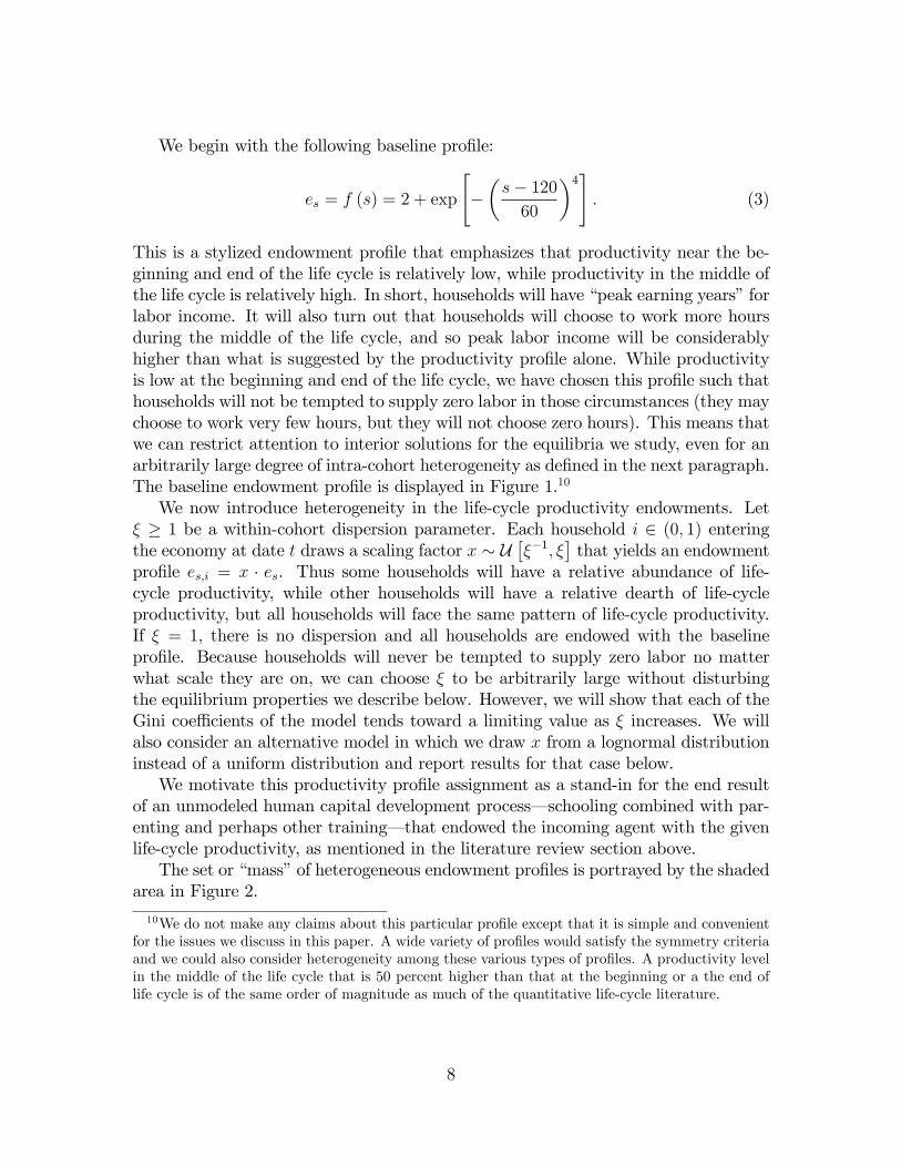
Figure 6: Distribution of net asset holding by cohort (shaded area) and a typical netasset profile by age (line).

years, reaching a period of peak net asset holdings during the second half of thelife cycle. Households that have different life-cycle productivity endowments followidentical life-cycle net asset accumulation and decumulation patterns, but scaled upor down according to their value of x. Financial wealth must sum to zero as theclosed economy equilibrium condition.Figure 6 shows the net asset-holding profiles by age.As the economy evolves, borrowing and lending both increase in proportion to

increases in w (t). That is, each cohort’s net asset holding shifts up or down accordingto the value of that period’s real wage w (t).

3.6 Remarks on a lognormal scaling factor

We have presented a characterization of the model equilibrium based on drawing thescaling factor x each period from a uniform distribution. Drawing the scaling factorx from a lognormal distribution may be more aesthetically appealing, as it allowsfor arbitrarily rich and arbitrarily poor households and concentrates more householdsat a particular part of the life-cycle productivity profile distribution, which mightbe thought of as the “ordinary” life-cycle productivity profile. Our specificationcan accommodate this extension because agents will always choose interior solutionsindependently of the scale of the life-cycle productivity profile. However, we have

20

found that the Gini coefficients implied by this type of scaling are very similar to thecase where the scaling factor x is drawn from a uniform distribution. Accordingly,we do not discuss this case further in this version of the paper.

4 Gini coefficients

We now turn to a discussion of Gini coefficients based on the distributions displayedabove where the scaling factor x is drawn from a uniform distribution. While thismodel is too simple to completely characterize the U.S. data, we hope to generatesome confidence that a model in this class could begin to confront the observed levelof heterogeneity in wealth, income, and consumption. In the U.S. data, it is widelybelieved that the consumption Gini is less than the income Gini, which is, in turn,less than the financial wealth Gini. The model naturally produces this ordering.We begin with targets in the U.S. data. For the consumption Gini, we follow

Heathcote, Perri, and Violante (2010) and set GC,U.S. = 32%. The income Gini isthe most widely measured. We take the value reported by the Congressional BudgetOffice (2016), for income pre-taxes and transfers, of GY,U.S. = 51%. Finally, we usethe financial wealth Gini for the U.S. reported by Davies, Sandström, Shorrocks, andWolff (2011), GW,U.S. = 80%.We approximate all of the probability density functions (PDFs) from the model

with Chebyshev polynomials17 and compute the corresponding Gini coefficients asfollows:

Gx =1

µx

∫ +∞

0

Fx (y) [1− Fx (y)] dy,

where µx denotes the mean of the variable of interest, x, and Fx denotes the cumu-lative distribution function of x. Figure 7 portrays the PDFs for our model.The Gini coefficients for our model are as follows:

• endowment distribution: GE = 33.5%,

• consumption distribution: GC = 31.8%,

• income distributions: GY1 = 56.2%, GY2 = 51.6%, GY3 = 59.6%,

• wealth distribution: GW = 72.7%.

These figures suggest that it is not difficult to obtain Gini coefficients for thismodel that are close to those observed in the U.S. data. Not surprisingly, the moredispersion there is in endowment profiles, ξ, the higher are the Gini coefficients (seeFigure 8).The Gini coefficients of the distribution of endowments and wealth are invariant to

η, because η does not affect endowments or net asset accumulation decisions. Similarly

17See Driscoll, Hale, and Trefethen (2014).

21

0 100

0.05

0.1Endowment

0 50

0.5

1Labor income

0 20

0.5

Consumption

0 1000

0.01

0.02Wealth

Figure 7: PDFs of endowment, labor income, consumption, and wealth. The wealthsubplot omits a mass point (121/241) at 0.

2 4 6 8 100

0.5

1

Figure 8: Gini coefficients of wealth (red), max (a/P, 0); labor income (blue),we (1− l); and consumption (green) as functions of endowment dispersion, ξ.

22

2 4 6 8 100.2

0.4

0.6

0.8

1

0.25

0.3

0.35

0.35

0.4

0.4 0.450.45 0.50.5 0.550.55

Figure 9: Gini coefficient of the distribution of labor income for different values of ξand η.

the Gini coefficient for the consumption distribution is independent of η because ηscales consumption choices in the same way for all households (see equation (25))without affecting the distribution. As illustrated in Figure 9, the Gini coefficient ofthe distribution of labor income is decreasing in η.

5 Characterizing monetary policy

In this section we turn to the issue of characterizing the nature of optimal monetarypolicy in this model. We have said that the monetary policymaker credibly followsthe price level rule (15) for all t. This rule is expressed in a compact form that canbe substituted directly into the households’ problems to deliver the complete marketssolution of the model. The rule turns non-state contingent nominal contracts intostate contingent contracts denominated in real terms. Thus the rule provides a formof insurance to credit market participants in the model, and the model equilibrium ischaracterized by complete markets with equity share contracting.18

Nevertheless, monetary policy is more commonly discussed in terms of a short-term nominal interest rate over which the monetary authority is assumed to havecomplete control. We now turn to an interpretation of the model along these lines.The nominal contracts in the model are set by market participants with an under-

standing of the price level rule, and the price level rule is adhered to by the monetary

18The price level rule (15) is not the unique rule that can restore complete markets. Azariadis,Bullard, Singh, and Suda (2018) present an alternative rule that delivers the complete marketsallocation.

23

authority with an understanding that nominal contracting is occurring. To expressmonetary policy in the common language of short-term nominal interest rates wecan find the fixed point of this process and then illustrate the general equilibriumresponses to macroeconomic shocks.To begin, the contract nominal interest rate (12) can be understood as the ex-

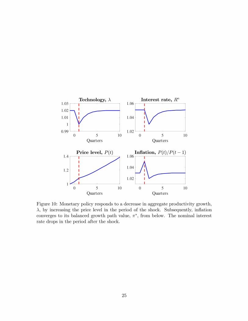
pected rate of nominal GDP growth. The Wicksellian natural real rate of interest inthis economy can be understood as the real rate of growth of the economy (λ) . Itis this growth rate that is the stochastic element of the equilibrium. The monetarypolicy (15) is to set the price level in a countercyclical manner such that the nominalinterest rate contract, which is also the expected rate of nominal GDP growth, isalways ratified ex post. This makes the real interest rate equal to the Wickselliannatural rate of interest. This aspect of policy is the same as in New Keynesian models.It follows from this discussion that in the special case of serially uncorrelated

shocks (ρ = 0), the expected rate of real GDP growth will never change, and hence,because of the monetary policy, the expected rate of nominal GDP growth will neverchange either. Thus the policy in this particular circumstance could be characterizedas a nominal interest rate peg or, equivalently, perfect nominal GDP targeting. Ineach period, as real shocks occur, the price level is adjusted in such a way thatthe previous period’s expectation of nominal GDP, and hence the contract nominalinterest rate, turns out to be exactly correct. The economy never deviates from thenominal GDP path desired by policymakers.In the more general case of serially correlated shocks (ρ > 0), this extreme result is

modified. If the growth rate of the economy falls or rises persistently, the expectationof future nominal GDP growth will fall or rise persistently. This means that thecontract nominal interest rate will also fall or rise persistently. The price level rule (15)still calls for countercyclical price level movements that ratify the previous period’sexpectations. However, these expectations are now themselves moving persistentlyhigher or lower depending on the shocks to the real growth rate λ.We can still think ofthe policy as a form of nominal GDP targeting, but one that returns the economy tothe desired nominal GDP path more slowly because of the persistence of real shocks.These considerations suggest the following observations for interpreting the sug-

gested price level rule policy in nominal interest rate terms. In general, the policy-maker controlling a short-term nominal interest rate wants to follow the natural rateof real growth in the economy as part of the optimal policy. In particular. a recessionis associated with lower nominal and real interest rates as part of the optimal policy.The policy also always ratifies the nominal interest rate contract, so that nominalinterest rates do not react in the period of the shock but only one period later. Inthe period of the shock, inflation moves higher as part of the counter-cyclical pricelevel movement associated with the optimal policy. These features are illustrated inFigure 10.Koenig (2012) discusses the relationship between nominal GDP targeting and

more familiar Taylor-type policy rule approaches to monetary policy. He argues that

24

0 5 10

Quarters

0.99

1

1.01

1.02

1.03

0 5 10

Quarters

1.02

1.04

1.06

0 5 10

Quarters

1

1.2

1.4

0 5 10

Quarters

1.02

1.04

1.06

Figure 10: Monetary policy responds to a decrease in aggregate productivity growth,λ, by increasing the price level in the period of the shock. Subsequently, inflationconverges to its balanced growth path value, π∗, from below. The nominal interestrate drops in the period after the shock.

25

the two approaches are “close cousins,” but from a perspective in which sticky pricesprovide the key nominal friction. We hope to address this issue in the NSCNC contextin future versions of this model.

6 Conclusion

In this paper we study an economy with “massive” heterogeneity and optimal mone-tary policy. NSCNC is the key friction in the economy. The policymaker can providea type of insurance against aggregate shocks for all households in the model, whetherthey are rich or poor and whether they hold net assets or are net borrowers. This ap-proach may provide an interesting baseline equilibrium for thinking about monetarypolicy in heterogeneous agent economies. The model is too simple to try to use it toaggressively confront the U.S. data on heterogeneous households, but we neverthelesscharacterize an illustrative benchmark equilibrium in which the Gini coefficients inthe model begin to approach those in the U.S. data on dimensions of inequality withrespect to income, consumption, and financial wealth.

References

Aiyagari, S. R. (1994): “Uninsured Idiosyncratic Risk and Aggregate Saving,”Quarterly Journal of Economics, 109(3), 659—684.

Auclert, A. (2019): “Monetary Policy and the Redistribution Channel,” AmericanEconomic Review, forthcoming.

Azariadis, C., J. Bullard, A. Singh, and J. Suda (2018): “Incomplete CreditMarkets and Monetary Policy,” University of Sydney, unpublished manuscript.

Bhandari, A., D. Evans, M. Golosov, and T. Sargent (2018): “Inequality,Business Cycles and Monetary-Fiscal Policy,” NBER Working Paper No. 24710.

Braun, R. A., and T. Oda (2015): “Real Balance Effects When the NominalInterest Rate is Zero,” Federal Reserve Bank of Atlanta, unpublished manuscript.

Bullard, J. (2014): “Comment on Debt and Incomplete Financial Markets: A Casefor Nominal GDP Targeting,” Brookings Papers on Economic Activity, Spring, 362—368.

Bullard, J., and J. Feigenbaum (2007): “A Leisurely Reading of the Life-CycleConsumption Data,” Journal of Monetary Economics, 54(8), 2305—2320.

Bullard, J., and A. Singh (2019): “Nominal GDP Targeting With HeterogeneousLabor Supply,” Journal of Money, Credit and Banking, forthcoming.

26

Chari, V. V., and P. J. Kehoe (1999): “Optimal fiscal and monetary policy,” inHandbook of Macroeconomics, ed. by J. B. Taylor, and M. Woodford, vol. 1, PartC, chap. 26, pp. 1671—1745. North Holland, Amsterdam.

Congressional Budget Office (2016): “The Distribution of Household In-come and Federal Taxes, 2013,” https://www.cbo.gov/sites/default/files/114th-congress-2015-2016/reports/51361-householdincomefedtaxes.pdf.

Davies, J. B., S. Sandström, A. Shorrocks, and E. N. Wolff (2011): “TheLevel and Distribution of Global Household Wealth,” Economic Journal, 121(551),223—254.

Debortoli, D., and J. Galì (2018): “Monetary Policy with Heterogeneous Agents:Insights from TANK Models,” CREI, unpublished manuscript.

Doepke, M., andM. Schneider (2006): “Inflation and the Redistribution of Nom-inal Wealth,” Journal of Political Economy, 114(6), 1069—1097.

Driscoll, T. A., N. Hale, and L. N. Trefethen (eds.) (2014): Chebfun Guide.Pafnuty Publications, Oxford.

Eggertson, G. B., N. R. Mehrotra, and J. A. Robbins (2018): “A Modelof Secular Stagnation: Theory and Quantitative Evaluation,” American EconomicJournal: Macroeconomics, forthcoming.

Feng, Z., and M. Hoelle (2017): “Indeterminacy in Stochastic Overlapping Gen-erations Models: Real Effects in the Long Run,” Economic Theory, 63(2), 559—585.

Galì, J. (2014): “Monetary Policy and Rational Asset Price Bubbles,” AmericanEconomic Review, 104(3), 721—752.

(2018): “The State of New Keynesian Economics: A Partial Assessment,”Journal of Economic Perspectives, 32(3), 87—112.

Garriga, C., F. E. Kydland, and R. Šustek (2017): “Mortgages and MonetaryPolicy,” Review of Financial Studies, 30(10), 3337—3375.

Heathcote, J., F. Perri, and G. L. Violante (2010): “Unequal We Stand:An Empirical Analysis of Economic Inequality in the United States, 1967—2006,”Review of Economic Dynamics, 13(1), 15—51.

Huggett, M., G. Ventura, and A. Yaron (2011): “Sources of Lifetime Inequal-ity,” American Economic Review, 101(7), 2923—2954.

Kaplan, G., B. Moll, and G. L. Violante (2018): “Monetary Policy Accordingto HANK,” American Economic Review, 108(3), 697—743.

27

Ko, D.-W. (2015): “Inequality and Optimal Monetary Policy,” Rutgers University,unpublished manuscript.

Koenig, E. F. (2012): “All in the Family: The Close Connection Between Nominal-GDP Targeting and the Taylor Rule,” Staff Paper No. 17, Federal Reserve Bankof Dallas.

(2013): “Like a Good Neighbor: Monetary Policy, Financial Stability, andthe Distribution of Risk,” International Journal of Central Banking, 9(2), 57—82.

McKay, A., E. Nakamura, and J. Steinsson (2016): “The Power of ForwardGuidance Revesited,” American Economic Review, 106(10), 3133—3158.

Sheedy, K. D. (2014): “Debt and Incomplete Financial Markets: A Case for Nom-inal GDP Targeting,” Brookings Papers on Economic Activity, Spring, 301—361.

(2018): “Taking Away the Punch Bowl: Monetary Policy and FinancialInstability,” London School of Economics, unpublished manuscript.

Sterk, V., and S. Tenreyro (2018): “The Transmission of Monetary PolicyThrough Redistributions and Durable Purchases,” Journal of Monetary Economics,99, 124—137.

Werning, I. (2014): “Comment on Debt and Incomplete Financial Markets: A Casefor Nominal GDP Targeting,” Brookings Papers on Economic Activity, Spring, 368—372.

28

A Appendix

The model features heterogeneous households and an aggregate shock, so that theevolution of the asset-holding distribution in the economy is part of the descriptionof the equilibrium. This would normally require numerical computation. However,symmetry, log preferences, and other simplifying assumptions allow solution by “pen-cil and paper” methods. In this Appendix we outline this solution in some detail. Akey feature of the solution is that the asset-holding distribution will be linear in thecurrent real wage w (t), and so will simply shift up and down with changes in w (t).Another key feature of the solution will be that the stochastic real rate of return onasset holdings will be equal to the stochastic real output growth rate period by pe-riod. We do not claim uniqueness of this equilibrium, but we regard the equilibriumwe isolate as a natural focal point for this analysis.19

We guess and verify a solution given a particular price rule for P employed by themonetary authority.(1) We first propose the state contingent policy rule for the price level P and

assume that this rule is perfectly credible for all time t ∈ (−∞,+∞) .(2) We then state the problem of household i entering the model at an arbitrary

date t under the NSCNC friction. We substitute the proposed policy rule directlyinto this problem.(3) We solve this problem and show that date t choices for ct,i (t) and `t,i (t) for this

household depend only on date t information and not on expectations of the futurestochastic evolution of wages, reflecting the insurance provided by the policymaker.(4) We argue that suitable adaptations of this same result also apply for all house-

holds that entered the economy at dates earlier than date t with various life-cycleproductivity profiles i and with non-zero net asset holdings brought into date t.(5) We then show that the general equilibrium market clearing condition, which

is that net asset holding sums to zero across the economy, is met given the derivedhousehold behavior. Thus we have identified an equilibrium of the stochastic economyin which the stochastic gross real interest rate R (t, t+ 1) is equal to the stochasticgross rate of growth of real output in the economy, λ (t, t+ 1) , for all t.Given our assumption, all household choices will be interior, meaning in particular

that leisure choices will obey 0 < `t,i (t+ s) < 1 for all s, i. We verify this aspect ofthe solution later.Step 1. A household i entering the economy at date t faces uncertainty about

income over its life cycle because it does not know what the real wage level is goingto be in the future. The proposed state contingent policy rule provides insurance

19See Feng and Hoelle (2017) for a recent discussion and analysis. Typical quantitative-theoreticapplications in the area of stochastic overlapping generations would be unable to address the issuesbrought out by the Feng and Hoelle analysis.

29

against this uncertainty and is given by

P (t+ 1) =Rn (t, t+ 1)

λr (t, t+ 1)P (t) (26)

for all t, with P (0) > 0.Step 2. We first consider households i entering the economy at date t. The

problem of these agents is

max{ct,i(t+s),`t,i(t+s)}Ts=0

Et[

T∑

s=0

[η ln ct,i (t+ s) + (1− η) ln `t,i (t+ s)] (27)

subject to the lifetime budget constraint (which is an aggregation of the sequence ofperiod budget constraints the agent faces) given by

ct,i (t) +

T∑

s=1

(P (t+ s)

P (t)

ct,i (t+ s)

Rn (t, t+ s)

)≤

e0w (t) [1− `t,i (t)] +

T∑

s=1

(P (t+ s)

P (t)

es,iw (t+ s) (1− `t,i (t+ s))

Rn (t, t+ s)

), (28)

where

Rn (t, t+ s)=s∏

j=1

Rn (t+ j − 1, t+ j) . (29)

Substitution of the policy rule into the budget constraint for these households yieldsa new version of the lifetime budget constraint,

ct,i (t) +T∑

s=1

(ct,i (t+ s)

∗ (t, t+ s)

)≤ w(t)

T∑

s=0

es (1− `t,i (t+ s)) , (30)

where

Λ (t, t+ s) =s∏

j=1

λr (t+ j − 1, t+ j) . (31)

We note that by the timing protocol of this model, w (t) is known by the household atthe time this problem is solved. If the model had no NSCNC friction–so that assetholdings were expressed in real instead of nominal terms–and we simply replacedall gross real interest rates with gross output growth rates, we would obtain thesame lifetime budget constraint expression. Therefore, if the derived behavior fromthis problem meets the general equilibrium condition below, we can claim that theequilibrium is that the gross real interest rate R (t, t+ 1) = λ (t, t+ 1) ∀t.

30

Step 3. The household i then solves this problem, where µi is the multiplieron the life-time budget constraint. The sequence of FONCs for s = 0, 1, ..., T withrespect to consumption is given by

η

ct,i (t)= µi, (32)

η

ct,i (t+ s)=

µiΛ (t, t+ s)

. (33)

These conditions imply that the household i state contingent consumption plan fordates t+s, s = 1, ..., T, depends on the realizations of future shocks to the productivitygrowth rate, λ:

ct,i (t+ s) = Λ (t, t+ s) ct,i (t) . (34)

The sequence of FONCs for s = 0, 1, ..., T with respect to ` is

1− η

`t,i (t+ s)= µiw (t) es,i. (35)

We combine each of these with the corresponding FONC for consumption to give thefollowing choices for leisure for s = 0, 1, ..., T :

`t,i (t+ s) =1− η

η

ct,i (t)

w (t) es,i. (36)

We can then substitute back for leisure into the budget constraint

(T + 1)ct,i (t) ≤ w(t)

T∑

s=0

es,i

(1−

1− η

η

ct,i (t)

w (t) es,i

), (37)

orct,i (t) = ηw (t) ei, (38)

where es,i ≡∑T

s=0 es,i/ (T + 1) denotes the average endowment over the life cyclefor agents with productivity profile i. We conclude that the choice for first-periodconsumption, ct,i (t), depends on the desirability of consumption versus leisure, η; theproductivity profile assigned to this agent ei; and today’s wage w (t) alone (and noton any future expected wages).The amount of leisure chosen at date t and the amount chosen in the future

depends on the household’s position in the life cycle. These amounts are given by

`t,i (t+ s) = (1− η)eies,i

= (1− η)e

es∀i, (39)

where e =∑T

s=0 es/ (T + 1) is the average baseline endowment. If η = 1, the house-hold will choose no leisure. If η → 0 and e0,i = eT,i are small enough, then `t,i (t)

31

and `t,i (t+ T ) could be larger than 1, meaning the households would supply no la-bor on those dates. This would violate our interior solution assumption. We assumee0,i = eT,i � 0 and η sufficiently large to maintain interior leisure choices.This household will carry some nominal asset position at,i (t) into the next period.

The date t real value of this position is given by

at,i (t)

P (t)= e0,i [1− `t,i (t)]w (t)− ct,i (t) (40)

= e0,i

(1− (1− η)

eie0,i

)w (t)− ηw (t) ei (41)

= w (t) (e0,i − ei) . (42)

This asset position is linear in the real wage w (t).Step 4. There are also households i that entered the economy at dates t− 1, t−

2, · · · , t−T that would solve a similar problem. These households bring nominal assetholdings at−1,i (t− 1) , at−2,i (t− 1) , · · · , at−T,i (t− 1) , respectively, into the currentperiod and have a shorter remaining horizon in their life cycle. Here we show thesolution to a household problem for household i that entered the economy at datet − 1. In particular, we show that the net asset-holding choice at date t, at−1,i (t) ,continues to be linear in the current real wage w (t). We then infer solutions for allof the other household problems for households i that entered the economy at datest− 2, · · · , t− T .Household i that entered the economy at date t− 1 solves this problem at date t :

max{ct−1,i(t+s),`t−1,i(t+s)}

T−1s=0

Et

T−1∑

s=0

[η ln ct−1,i (t+ s) + (1− η) ln `t−1,i (t+ s)] (43)

subject to the lifetime budget constraint

ct−1,i (t) +T−1∑

s=1

(P (t+ s)

P (t)

ct−1,i (t+ s)

Rn (t, t+ s)

)≤ e1w (t) [1− `t−1,i (t)]

+

T−1∑

s=1

(P (t+ s)

P (t)

es+1,iw (t+ s) (1− `t−1,i (t+ s))

Rn (t, t+ s)

)+Rn (t− 1, t) at−1,i (t− 1)

P (t).

(44)

In this “remaining lifetime” budget constraint, we can see from Step 2 above whatthe (nominal) value of at−1,i (t− 1) must have been from last period, namely

at−1,i (t− 1) = P (t− 1)w (t− 1) (e0,i − ei) . (45)

We can therefore find the value of Rn (t− 1, t) at−1,i (t− 1) to be

Rn (t− 1, t) at−1,i (t− 1) = Rn (t− 1, t)P (t− 1)w (t− 1) (e0,i − ei) . (46)

32

We can use the policy rule P (t) = Rn(t−1,t)λr(t−1,t)

P (t− 1) and the law of motion for w (t)to obtain

Rn (t− 1, t) at−1,i (t− 1) = Rn (t− 1, t)P (t)λr (t− 1, t)

Rn (t− 1, t)

w (t)

λr (t− 1, t)(e0,i − ei)

= P (t)w (t) (e0,i − ei) . (47)

Therefore, the entire real-valued term is given by

Rn (t− 1, t) at−1,i (t− 1)

P (t)= w (t) (e0,i − ei) . (48)

This term is linear in w (t), and since it enters the budget constraint in a lump-sumfashion, it does not affect the FONCs.We now substitute the policy rule into the rest of the budget constraint to obtain

a new version of the remaining lifetime budget constraint:

ct−1,i (t) +

T−1∑

s=1

(ct,i (t+ s)

Λ (t, t+ s)

)≤ w(t)

T−1∑

s=0

es+1 (1− `t−1,i (t+ s)) . (49)

The FONCs for s = 1, ..., T − 1 with respect to consumption can be expressed as

η

ct−1,i (t)= µi, (50)

η

ct−1,i (t+ s)=

µiΛ (t, t+ s)

, (51)

which impliesct−1,i (t+ s) = Λ (t, t+ s) ct−1,i (t) . (52)

The FONCs for s = 0, ..., T − 1 with respect to ` are

1− η

`t−1,i (t+ s)= µiw (t) es+1,i. (53)

We combine each of these with the corresponding FONC for consumption to give thefollowing choices for leisure for s = 0, ..., T − 1,

`t−1,i (t+ s) =1− η

η

ct−1,i (t)

w (t) es+1,i. (54)

We can now substitute back into the remaining life budget constraint. This can bewritten as

Tct−1,i (t) = w(t)

[T∑

s=1

es,i

(1−

1− η

η

ct−1,i (t)

w (t) es,i

)+

T

T + 1e0,i −

1

T + 1

T∑

s=1

es,i

]

, (55)

33

orct−1,i (t) = ηw (t) ei, (56)

which is linear in w (t).Equations (38) and (56) show that agents born at different dates but sharing the

same productivity profile i will consume the same amount at date t. Similar logicapplies for agents born at earlier dates t− 2, ..., t− T. This demonstrates the “equityshare contracting” feature of the equilibrium.Household i would then also have a desired real net asset position:

at−1,i (t)

P (t)= e1,iw (t) (1− `t−1,i (t))− ct−1,i (t) +

Rn (t− 1, t) at−1,i (t− 1)

P (t)

= (e0,i + e1,i − 2ei)w (t) . (57)

For all other households i at date t who entered the economy at date t−2, t−3, ..t−T,consumption and net assets at date t will also be linear in w(t).Step 5. The general equilibrium condition is that net assets sum to zero,

0 =T−1∑

s=0

at−s (t)

P (t), (58)

or equivalently that

0 =

T−1∑

s=0

at−s (t) . (59)

Suppose T = 2. We have seen above that

at,i (t)

P (t)= w (t) (e0,i − ei) (60)

and thatat−1,i (t)

P (t)= (e0,i + e1,i − 2ei)w (t) . (61)

The general equilibrium condition can therefore be written as

w (t) (e0,i − ei) + (e0,i + e1,i − 2ei)w (t) = 0 (62)

w (t) [(e0,i − ei) + (e0,i + e1,i − 2ei)] = 0 (63)

w (t) [e0,i + e1,i + e0,i − 3ei] = 0 (64)

w (t) [e0,i + e1,i + e0,i − (e0,i + e1,i + e2,i)] = 0. (65)

This last line will equal zero if e0,i = e2,i ∀i, which is the symmetry condition con-cerning life-cycle productivity profiles we have imposed on the model. Similar logicapplies for T > 2.

34

The policy rule we imposed in Step 1 modified the agents’ problems in Steps2, 3, and 4. As noted above, these modified problems were exactly the same onesthat would have been generated had there been no nominal friction in the modeland we had instead written the model entirely in real terms and guessed that modelequilibrium would be characterized by the equality of the real interest rate and thereal output growth rate at each date. The implied behavior of the households showsin Step 4 that this guess turns out to be correct. We conclude that the stochasticequilibrium is characterized by R (t− 1, t) = λ (t− 1, t) ∀t.

35