Research Division Federal Reserve Bank of St. Louis Working Paper Series

Schools and Stimulus

Bill Dupor and

M. Saif Mehkari

Working Paper 2015-004A

http://research.stlouisfed.org/wp/2015/2015-004.pdf

March 2015

FEDERAL RESERVE BANK OF ST. LOUIS Research Division

P.O. Box 442 St. Louis, MO 63166

______________________________________________________________________________________

The views expressed are those of the individual authors and do not necessarily reflect official positions of the Federal Reserve Bank of St. Louis, the Federal Reserve System, or the Board of Governors.

Federal Reserve Bank of St. Louis Working Papers are preliminary materials circulated to stimulate discussion and critical comment. References in publications to Federal Reserve Bank of St. Louis Working Papers (other than an acknowledgment that the writer has had access to unpublished material) should be cleared with the author or authors.

Schools and Stimulus∗

Bill Dupor†and M. Saif Mehkari‡

March 10, 2015

Abstract

This paper analyzes the impact of the education funding component of the 2009 AmericanRecovery and Reinvestment Act (the Recovery Act) on public school districts. We use cross-sectional differences in district-level Recovery Act funding to investigate the program’s impacton staffing, expenditures and debt accumulation. To achieve identification, we use exogenousvariation across districts in the allocations of Recovery Act funds for special needs students.We estimate that $1 million of grants to a district had the following effects: expendituresincreased by $570 thousand, district employment saw little or no change, and an additional$370 thousand in debt was accumulated. Moreover, 70% of the increase in expenditures camein the form of capital outlays. Next, we build a dynamic, decision theoretic model of a schooldistrict’s budgeting problem, which we calibrate to district level expenditure and staffing data.The model can qualitatively match the employment and capital expenditure responses from ourregressions. We also use the model to conduct policy experiments.

Keywords: fiscal policy, K-12 education, the American Recovery and Reinvestment Act of 2009.

JEL Codes: D21, D24, E52, E62.

∗The authors thank Peter McCrory for helpful research assistance. A repository containing government documents, data

sources, a bibliography, and other relevant information pertaining to the Recovery Act is available at billdupor.weebly.com.

The analysis set forth does not reflect the views of the Federal Reserve Bank of Saint Louis or the Federal Reserve System.

First draft: October 2014.†Federal Reserve Bank of St. Louis, william.d.dupor@stls.frb.org, billdupor@gmail.com.‡University of Richmond, smehkari@richmond.edu.

1

1 Introduction

The 2009 Recovery Act was signed into law with a primary goal of creating and saving millions

of jobs during and following the most recent recession. A large share of the appropriations from

the act was made as grants. Public school districts constituted one of the largest groups of these

recipients, receiving $64.7 billion in Department of Education Recovery Act funds.1,2

The act’s education component has been touted as one of the success stories by the law’s

supporters. Shortly after its passage, Vice President Joe Biden stated that funds from the act would

“help to keep outstanding teachers in America’s schools.”3 According to the Executive Office of the

President of the United States (2009), “the rapid distribution of SFSF [State Fiscal Stabilization

Funds] funding helped fill the gaps and avert layoffs of essential personnel in school districts and

universities across the nation.” The act’s official website, Recovery.gov, tracked the number of jobs

which were payrolled by the act’s funds using surveys of recipient organizations. The Council of

Economic Advisers (various quarterly reports) used the jobs counts data from these surveys as

evidence of the act’s success.4 According to these reports, Department of Education Recovery Act

dollars alone directly created and saved over 750 thousand jobs during the first two school years

following its passage.5

This paper analyzes the act’s impact on schools using cross-sectional differences in district-level

Recovery Act grants and expenditures, staffing and debt accumulation. We compare the behavior

of districts receiving relatively little grant money to those of districts receiving plenty of grant

money. From this comparison, we infer what all districts would have done had the act’s grants not

been available.

To address the potential endogenity of spending, we employ two instruments. Our first instru-

ment is the ratio of the number of special needs students relative to overall students in each district.

Our second instrument is the Recovery Act dollars received by a district through the act’s Special

Education Fund (SEF). The SEF was one category of the Recovery Act education component, con-

stituting one-fifth of the education grants. Its allocation across districts was determined primarily

by the requirement that districts finance their special needs programs. Although each instrument

is highly correlated with overall Recovery Act education spending, each is plausibly uncorrelated

with the short-run business cycle and tax revenue situations faced by school districts.

1This includes the Office of Special Education and Rehabilitative Services Special Education Fund ($12.2 billion)and the following Office of Elementary and Secondary Education programs: Education Stabilization funds ($42.0billion), Compensatory Education for the Disadvantaged ($12.4 billion), School Improvement Program ($0.7 billion).

2The federal government’s objectives for the each of the programs were explicit, and usually involved, in part, anattempt to stimulate economic activity. For example, “Among other things, the Education Stabilization funds maybe used for activities such as: paying the salaries of administrators, teachers, and support staff; purchasing textbooks,computers, and other equipment,” according to a U.S. Dept. of Education (2009a) implementation guidance.

3See Biden (2011).4See also Congressional Budget Office (various quarterly reports).5See Table A.1 for a quarterly breakdown of the payroll count data extracted from Recovery.gov. Here, a job is

measured as lasting one year and as a “full-time equivalent” of one respective position.

2

We have four main findings. First, the grants had either zero or else a small education jobs

impact. Each $1 million of aid to a district resulted in roughly 1.5 additional jobs at that district.

The point estimate implies that, in the first two school years following passage, the act increased

education employment by 95,000 persons nationwide. Moreover, this estimate is not statistically

different from zero.

We find no evidence that the grants increased the number of classroom teachers. Intuitively,

district administrators may have shown a strong preference for maintaining teacher-student ratios

and, to a lesser extent, staff-student ratios. As such, school officials may have found other margins

besides firing or hiring along which to cover shortfalls or spend surpluses.

Second, each $1 million of grants to a district increased its expenditures by $570 thousand.

Because districts already had substantial funds from local and state sources, the additional Recovery

Act funds were effectively fungible. Thus upon receipt of Recovery Act funds, state and local

funding sources may have reduced their own contributions to district funding which offset the act’s

grants.

Third, districts receiving grants tended to accumulate more debt. Fourth, roughly 70% of the

spending increase occurred as capital expenditures, i.e. construction and purchases of land, existing

structures and equipment. Why might districts have used these funds for capital improvement?

Since this aid was temporary, school districts may have smoothed the benefits of the aid over time

by making long-lived physical investments. In Section 4, we build and calibrate a model of dynamic

decision making by a forward-looking school district. We show that the small employment effect

and relatively large investment effect falls out of a fully specified and realistic dynamic programming

problem.

We also use our theoretical model as a laboratory to understand the effect of different types

of policy. Our main finding is that forcing school districts to use all the stimulus money on labor

has no additional effect on the employment outcome. School districts that are forced to only use

stimulus money on employment reduce the spending they do on labor from state and local funding

sources and substitute this shortfall with stimulus money, leaving the net employment outcome

unchanged. We show that an alternative policy where school districts are required to spend most

of their revenue (both from stimulus plus state and local sources) has a more significant effect on

employment.

With respect to existing work, there is almost no economic research on the act’s education

component. Two exceptions are, Dinerstein, et.al. (2013), who study the impact of the Act on

universities, and Chakrabart and Setren (2011), who examine the impact of the recession and the

early part of the Recovery Act on school districts in the state of New York. More generally, other

studies using microeconomic evidence that study the overall Recovery Act’s impact have focused

mainly on economy-wide labor market outcomes. These include Chodorow-Reich et al. (2012),

Conley and Dupor (2013), Dupor and McCrory (2015), Feyrer and Sacerdote (2012) and Wilson

3

(2012).

Another line of research studies how federal grants to schools influence school spending. Gor-

don (2004) studies the impact of additional federal grants to school districts serving economically

disadvantaged children, through the No Child Left Behind Act of 2001. She finds that, although

the additional federal grants initially caused a dollar-for-dollar increase in school spending, over

time school districts offset those increases with reductions in their own contributions to education

funding.

Lundqvist, Dahlberg and Mork (2014) study the impact of intergovernmental grants to local

governments in Sweden and find that the grants do not stimulate local public employment. Evans

and Owens (2007) study the extent to which federal grants to fund new police hires increased the

size of local police forces versus simply supplanted local funding. They found that for every four

officers payrolled by a grant, in an accounting sense, a police force actually only increased by a

little over two officers.

2 Empirical Analysis

2.1 The Data

The Sample

Our unit of observation is a public school district.6 During the 2010SY, there were 16,117 such

districts in the U.S. We restrict attention to districts with more than 500 student during that year.

After additionally excluding districts missing requisite data, we are left with 6,786 districts.7

Outcome Variables (∆Job-Years, ∆Expenditures and Debt accum)

Our first outcome variable measures school district employment. It is the change in employment

from a base of 2007SY over the first two school years in which the act was fully in effect, i.e. 2009SY

and 2010SY.8 Employed persons include teachers, aides, guidance counselors, librarians, district

administrators and other support staff. The data are self-reported by school districts in the annual

Common Core of Data Local Education Agency Universe Survey.

Let Yj,k denote employment by district j during school year k. Then,

∆Job-yearsj =1

Popj

2010∑k=2009

(Yj,k − Yj,2007)

6Our usage of the term school district is synonymous with the term “local education agency” (LEA), used in theeducation policy area. In the education policy jargon, our sample is made up of school districts and a small numberof regional educational service agencies.

7For example, we were forced to exclude data from all districts in Iowa, Montana, New Hampshire, Pennsylvaniaand Vermont because the Recovery Act spending information was reported in a manner that did not allow us tomatch them to school district spending and employment variables. We also excluded Hawaii because the entire stateis a single school district.

8We exclude the 2008SY because it includes only a few months in which the Recovery Act was in effect.

4

where Popj is the district j enrollment in the 2007SY.

From the annual Local Education Agency Finance Survey, we have data on total expenditures

Sj,t and debt. From these variables, we calculate our next two outcome variables. We measure

expenditure as the per student cummulative spending in the 2009SY and 2010SY relative to a

pre-act baseline.

∆Expenditurej =1

Popj

2010∑k=2009

(Sj,k − Sj,2007)

Debt accumulation is the change in the per student debt of a district over two school years

following the act’s passage.

Debt accumj =1

Popj(End of 2010SY Debtj − End of 2008SY Debtj)

Treatment Variable (V )

First, let Vj be the Recovery Act dollars outlaid to school district j, from enactment through

2011Q2.9 Outlaid dollars are defined as dollars paid by the federal government to a recipient

organization. These amounts are constructed using quarterly reports filed by recipients to the

web site FederalReporting.gov.10 Finally, we scale by the district enrollment and report values in

millions of dollars:

Vj =Vj

(1e+ 6)× Popj.

Nearly all of the education dollars authorized by the act were outlaid by the end of 2011Q2.

Instrument Variables (V SN and V SEF )

Since the allocation of the Act’s school funding was perhaps in part endogenous, we employ

instrumental variables. We have two instruments. Our first instrument is the per student value of

special education funding outlaid as part of the Recovery Act, defined as V SEFj , through 2011Q2.

The main channel by which the federal government supports special education is through the

Individuals with Disabilities Education Act (IDEA), a comprehensive statute originally passed in

1990 to ensure all students with disabilities are entitled to a free appropriate education. Most of

the Recovery Act special education money was tied to the IDEA program. While there are several

subprograms within IDEA, the lion’s share of monies comes through Part B of IDEA. The Recovery

Act funding formula follows the IDEA Part B formula.11

Recovery Act IDEA Part B grants were add-ons to regular annual IDEA Part B grants to

states. The national federal fiscal year (FFY) 2009 regular grant amount was $11.5 billion. The

9We use outlays through 2011Q2 because this aligns our Recovery Act data sample with the end of the 2010 schoolyear.

10After processing and data verification by the Recovery Accountability and Transparency Board, these data wereposted on the web site Recovery.gov. A user’s guide for these data is contained in Recovery Accountability andTransparency Board (2009).

11See U.S. Dept. of Education (2009b) and New America Foundation (2014).

5

first $3.1 billion (both from regular funding and the Recovery Act add-on) was divided up amongst

states so that they were guaranteed to receive their FFY1999 awards. Once this requirement was

met, the remaining part of the national award was allocated among the states according to the

following rule: “85% are allocated to States on the basis of their relative populations of children

aged 3 through 21 who are the same age as children with disabilities for whom the State ensures the

availability of a free appropriate public education (FAPE) and 15% on the relative populations of

children of those ages who are living in poverty.”12 The Recovery Act add-on totaled $11.3 billion.

Since, at the margin, the FY1999 requirements had already been met by the regular awards, every

Recovery Act dollar was in effect assigned across according to the 85/15 percent rule.

Next and importantly, we address how funds were assigned from state education agencies to

local education agencies (LEA). These initial allocations too were made at the federal level. Each

LEA was first allocated a minimum of its FFY1999 award.13 Beyond these minimums, which were

already met by the regular annual award amounts, a slightly different 85/15 rule was used. Within

each state, 85% of the dollars were allocated according to the share of school age children in the

LEA and 15% was allocated according the LEA’s childhood poverty rate. After this, states were

allowed to do reallocations as explained below. Before we explain how reallocations worked, we ask

whether the observed spending data at the within state level are explained by the simple formulary

rule.

Let Pj,s and Pj,s be the enrollment of students and students in poverty, respectively, in district

j and state s. Let IDEAj,s denote the total Recovery Act special needs funding in district j in

state s. Based on the above formula, the distribution of Recovery Act IDEA dollars would be

IDEAj,s =

(0.85× Pj,s∑Ns

i=1 Pi,s+ 0.15× Pj,s∑Ns

i=1 Pi,s

)IDEAs

Letting Ps and Ps denote the sum within state s of the two district level enrollment variables, we

can rewrite the above equation as:

IDEAj,sPj,s

=

[0.85× 1

Ps+ 0.15× 1

Ps

(Pj,sPj,s

)]IDEAs

Thus, within each state, the district level per pupil IDEA amount would be perfectly predicted by

the ratio of the low-income enrollment to the overall enrollment in the district if the simple formula

were used. Next we run state-level regressions to check this conjecture for the 46 state for which we

have fully reported IDEA amounts. The set of R2 from these regression are generally very low: 25

12See Enclosure B of U.S. Dept. of Education (2009b), which contains a description of how Recovery Act fundswere allocated across states.

13Federal code also describes how minimum awards are determined for LEAs created after 1999.

6

are less than 0.01. Only six of the R2 are greater than 0.1 and only one is greater than 0.3.14 This

tells us that other factors besides the poverty rate in each district are influencing the allocation of

IDEA funds.

This brings us to the rules for redistribution of dollars within state across LEAs, given by Code

of Federal Regulation 300.707(c)(1). It states:

If an SEA determines that an LEA is adequately providing FAPE to all children

with disabilities residing in the area served by that agency with State and local funds,

the SEA may reallocate any portion of the funds under this part ... to other LEAs in

the State that [are] not adequately providing special education and related services to

all children with disabilities residing in the area served by those LEAs.

Based on the legislation and given the low set of R2 above, we conclude that the primary reason

that IDEA money was allocated differently from the formulary rule is that some states were able

to meet their funding requirements of special needs students in some districts without drawing on

Recovery Act IDEA funds. Those funds were then reallocated to districts with additional funding

requirements for special needs students. Differences in funding requirements across districts were

likely due to factors, such as the number of special needs students, the types of disabilities and

their associated costs and the districts’ own funding contributions for providing the services to these

special needs students. Our exogenity assumption is that this set of factors driving redistributions

of IDEA funds is orthogonal to the error term in second stage equation.

Our second instrument is the ratio of the number of special needs students within a district

relative to the overall student enrollment in that district in 2007.15 Denote this variable as V SNj .

While the fraction of special needs students in a school district is likely to impact the Recovery Act

funding that a district receives, it is plausibly uncorrelated with the business cycle conditions and

tax revenue stress that the district faced.

Conditioning Variables (X)

We include the following conditioning variables, which we partition into three types:

• Pre-recession education variables: the 2007SY values of the teacher-student ratio, staff-

student ratio, expenditure per pupil; the change in debt per pupil over the 2007SY;

• Non-financial variables: the ratio of African American plus Hispanic enrollment to overall

enrollment, the natural log of enrollment, 7 region dummy variables, a constant;

• School district financials: the poverty rate, the fraction of revenue from local sources, the

cumulative change in revenue from non-federal sources

14As an additional measure, we include the poverty rate as an additional control in our estimation.15This data also comes from the Common Core of Data Universe Survey. As the data documentation explains,

special needs students are defined as “all students having a written Individualized Education Program (IEP) underthe Individuals with Disabilities Act (IDEA), Part B.”

7

Table 1: Summary statistics

Mean SD 10th perc. 90th perc.Change in total revenue (pp) 838.85 3186.31 -1778.23 3635.67Change in expenditure (pp) 689.81 5140.74 -3492.91 4976.10Recovery Act education spending (pp) 1013.20 766.98 446.04 1569.25Recovery Act IDEA spending (pp) 178.48 480.00 0.00 288.82Change in the wage bill (pp) 642.68 1397.71 -926.05 2256.92Change in the number of job-years (pp) -0.00 0.03 -0.03 0.02Debt accumulation (pp) 59.69 7443.66 -2381.30 2984.66Log of enrollment 7.83 1.09 6.55 9.32SY2007 values of:

Number of teachers (pp) 0.06 0.01 0.05 0.08Number of staff (pp) 0.12 0.03 0.08 0.16End of school year debt (pp)† 10.88 2.99 8.23 14.40One-year debt change (pp) 3653.55 30046.28 -3000.00 9662.00

Minority Rate 0.24 0.27 0.02 0.69Poverty Rate 0.03 0.02 0.01 0.05Self sufficiency ratio 0.41 0.20 0.19 0.71Total Recovery Act education spending = $36 billionTotal Recovery Act IDEA spending = $7 billionNumber of observations = 6,786

Notes: The unit of observation is a U.S. school district. The above sample excludes districts with enrollments less

than 500 in the 2010SY. † denotes variable has been divided through by 1000. IDEA, Individuals with Disabilities

Education Act; SD, standard deviation; pp, per pupil.

Details regarding a few of these variables are in order. The poverty rate is the number of young

persons living in poverty relative to the overall population of persons living within each school

district’s borders. The change in revenue from non-federal sources variable is given by

1

Popj

2010∑k=2008

(Rnonfedj,k −Rnonfedj,2007

)

where Rnonfedj,k is the district j revenue from nonfederal sources in school year k. The primary

nonfederal sources are from within the district and the state government.

Summary statistics for the variables in our analysis appear in Table 1.

2.2 The econometric model

We use two-stage least squares in estimation. The statistical model for the ∆Job-years equation is

Vj = θ1VSEFj + θ2V

SNj + ψXj + vj (2.1)

∆Job-yearsj = βJY Vj + γXj + εj

8

where Vj are the fitted values from the first-stage regression. The parameter of interest is

βJY . The statistical model for the other two outcome variables simply replaces ∆Job-yearsj with

∆Expenditurej or Debt Accumj . Our estimates are weighted by district enrollment and we report

robust standard errors.

3 Results

3.1 Benchmark results

The employment effect

Table 2 contains our benchmark estimates. We report the job-years response to grants in

column (i). The coefficient on education spending equals 1.47 (SE=1.32): Every $1 million in

grants increased district employment by 1.47 relative to a no Recovery Act baseline. Note that

our construction of the outcome variable is such that one job should be interpreted as lasting one

year. This estimate is not statistically different from zero, but estimated sufficiently precisely to

conclude that the jobs effect was small at best. At the upper end of the 95% confidence interval,

the employment effect was 4.05 persons per million dollars spent. We view this as quantitatively

small bearing in mind that the average education industry wage was roughly $50,000 during this

period.16 The estimates for other outcome variables, presented below, elucidate two reasons why

there was a small, if any, education jobs effect. First, a large portion of the grants did not translate

into greater district-level expenditures. Second, district level expenditures that did arise from the

grants were mainly used for capital expenditures.

Next, using the job-years response estimate, we calculate the implied total number of education

job-years resulting from the act’s education component. Taken at the upper end of its 95% confi-

dence interval, our estimate is that the effect was 260,000 jobs.17 As explained in the introduction,

this is substantially lower than the corresponding number based on payroll count data reported at

Recovery.gov.18

The bottom rows of Table 2 report key statistics from the first-stage regressions. The first-

stage results indicate that we have two strong instruments. The partial F -statistic is 78.93, with

a pointwise t-statistics of 4.29 for the special education student ratio instrument and 10.33 for the

Special Education Funds instrument.

Our jobs effect finding begs the question: Why were so few, if any, education jobs created

as a result of the act? One possibility is that district administrators viewed their staff, and in

particular teachers, as so important to their mission that districts receiving relatively little aid

16The mean annual wage for U.S. workers in the “Education, Training and Library” occupation was $49,530 in2009.

17We calculate this number by multiplying the 95% upper bound of the job-years coefficient confidence intervalby the cumulative total Recovery Act education spending through the 2010SY. This calculation assumes that thetreatment effect is the same for districts within our sample as those excluded from the sample.

18See Table A.1 for a tabulation of the Council of Economic Advisers payroll count data.

9

Table 2: Estimates of the impact on staff employment, expenditures and debt accumulation of $1million of Recovery Act education grants, benchmark results

∆ Job-years ∆ Expenditure Debt accum.(i) (ii) (iii)

Recovery Act education grant 1.47 570.10*** 340.63*($1 mil) (1.32) (196.60) (185.12)Ln(population) 0.04 148.93** -38.88

(0.55) (64.57) (97.72)Minority ratio -0.02*** 1.47*** 0.77**

(0.00) (0.36) (0.39)Poverty rate -0.03 -15.22*** 7.49

(0.04) (5.61) (10.62)Nonfederal spending change 1.62*** 632.00*** 78.36*

(0.23) (45.11) (44.11)Self-supporting school -0.01*** -1.21** -0.72district (0.00) (0.60) (0.68)Teachers per pupil, lag -0.05 67.66*** 27.08**

(0.15) (9.41) (12.92)Staff per pupil, lag -0.36*** 5.49 -12.39**

(0.04) (3.67) (5.13)Total expenditure per pupil, 0.00*** -0.00*** 0.00lag (0.00) (0.00) (0.00)Debt change, lag -0.00*** -0.00 0.00

(0.00) (0.00) (0.00)Region dummies Yes Yes YesNo. of Observations 6786 6786 6786First stage resultsSpecial Ed. ratio (t-stat) 4.29 4.29 4.29IDEA Recovery Act aid (t-stat) 10.33 10.33 10.33Partial F-stat 78.93 78.93 78.93

Notes: Each estimation also includes additional conditioning variables described in the text. The regressions are

enrollment weighted. Standard errors in parentheses. *** denotes 1% , ** 5% and * 10% significance. The expenditure

and debt accumulation variables are in units of thousands of dollars.

10

found ways to close budget gaps without firing many staff. Also, districts that received relatively

generous Recovery Act grants may have been less willing to hire new staff for risk that, once the

short-lived grants were spent, the new staff would need to be let go. Adjusting the capital outlays

was an alternative way to spend grant dollars. We provide empirical evidence of and theoretical

justification for a capital outlay response later in the paper.

If neither large grant nor small grant districts significantly adjusted their staff levels in re-

sponse to the shock, then we should expect our IV estimates to reflect a small jobs effect. An

absence of significant changes in staffing levels is consistent with narrative descriptions of districts’

responses to the most recent recession. Cavanaugh (2011) explains that school officials initially

responded to budget stress caused by the recession “at the periphery,” e.g., cutting travel, delaying

equipment upgrades as well as scaling back extracurricular activities, art and music programs. As

further evidence, based on surveys of school administrators, AASA (2012) lists many ways that

school administrators filled budget gaps during the period without firing employees. These include

furloughing personnel, eliminating or delaying instructional improvement initiatives, deferring text-

book purchases and reducing high cost course offering. While each of these may have marginally

reduced the quality of education services provided by the schools, the changes did not directly

impact the total number of district employees.

Note that if there was job creation outside of district employment, perhaps because of a “Keyne-

sian multiplier” effect, this is not reflected in our estimates because we examine only school district

employment.

The expenditure effect

Column (ii) of Table 2 reports estimates for the ∆Expenditure specification. The point estimate

on Recovery Act education spending equals 570 (SE=197) thousand. This implies that $1 million

of education grants resulted in an increase in expenditures of approximately $570 thousand over

the first two full school years following the act’s passage. Thus, only about one-half of aid to a

district actually translated into more expenditures in that district. One explanation for this result

may be that there was substantial “crowding-out” of local and state governments’ contribution to

public education when school districts received Recovery Act dollars.

This findings relates to previous research on whether federal grants crowd out state and local

spending. In a simple political economy model, Bradford and Oates (1971) shows conditions under

which crowding out occurs. Leduc and Wilson (2013) present evidence that crowding out was not

a problem for the highway component of the Recovery Act.

The debt accumulation effect

Column (iii) of Table 2 presents the results with debt accumulation per pupil over the two

years following the act’s passage as the outcome variable. The point estimate on the Recovery

Act spending variable is 340 (SE = 185) thousand. Based on the point estimate, districts which

11

received relatively more aid tended to increase their debt positions. The estimate is statistically

different from zero, but only at a 10% level.

3.2 Additional results

Table 3 gives the responses of the outcome variables for several variations on the benchmark spec-

ification. Panels A and B provide the weighted and unweighted specifications, respectively. The

first row contains the benchmark estimates. The “Ordinary least squares” row is identical to the

benchmark specification except we estimate via OLS rather than instrumental variables. The next

two rows estimate the model for each instrument separately. The final two rows sequentially drop

the region dummies and then drop all lagged variables.

Column (i) of Table 3 presents the job years estimates for all of the alternative specifications.

The majority of estimates are close to the benchmark one. There are three things worth noting.

First, not weighting by enrollment has very little effect on the estimate. Second, the OLS estimate

is very similar to our benchmark IV case. This suggests that the endogeniety problem is not severe

in this case.

Third, instrumenting with only the special education ratio generates a substantial increase in

the jobs as well as the expenditure effect relative to the benchmark specification. The job years

estimate increases to 8.04 (SE = 7.36). Note that we are unable to reject a zero jobs effect for this

specification. This specification results in the strongest jobs and expenditure effects of all of the

alternative estimated models. Interestingly, the large jobs and expenditure effects are diminished

substantially in the corresponding unweighted estimates (see panel B).

Column (ii) of Table 3 presents the total expenditure estimates. Recall that the coefficient is

interpreted as the thousands of dollars by which expenditures increase for a $1 million Recovery Act

education grant to the district. Thus, if the value is less than 1,000, then there is some “crowding

out” of the grants because part of the aid is not passing through to expenditures. The majority of

estimates are close to the benchmark one and exhibit substantial crowding out.

Column (iii) of Table 3 presents the debt accumulation estimates. The benchmark estimate

shows a statistically significant positive effect. All of the alternative specifications have a positive

point estimate, with roughly one-half being statistically different from zero. The only outliers are

the “special education instrument only” cases, both weighted and unweighted. The point estimates

for these specifications jump to $4.0 million and $8.5 million respectively. We view these values as

implausibly large.

Column (iv) of the table contains the partial F -statistic for each specification. None of the

values indicate a weak instrument problem, although the statistic is dramatically lower for the

“special education instrument only” specifications.

Next, we consider what type of education jobs were impacted. Did the grants create and

save teachers jobs or those of other employees? Table 4 presents the estimates for the benchmark

12

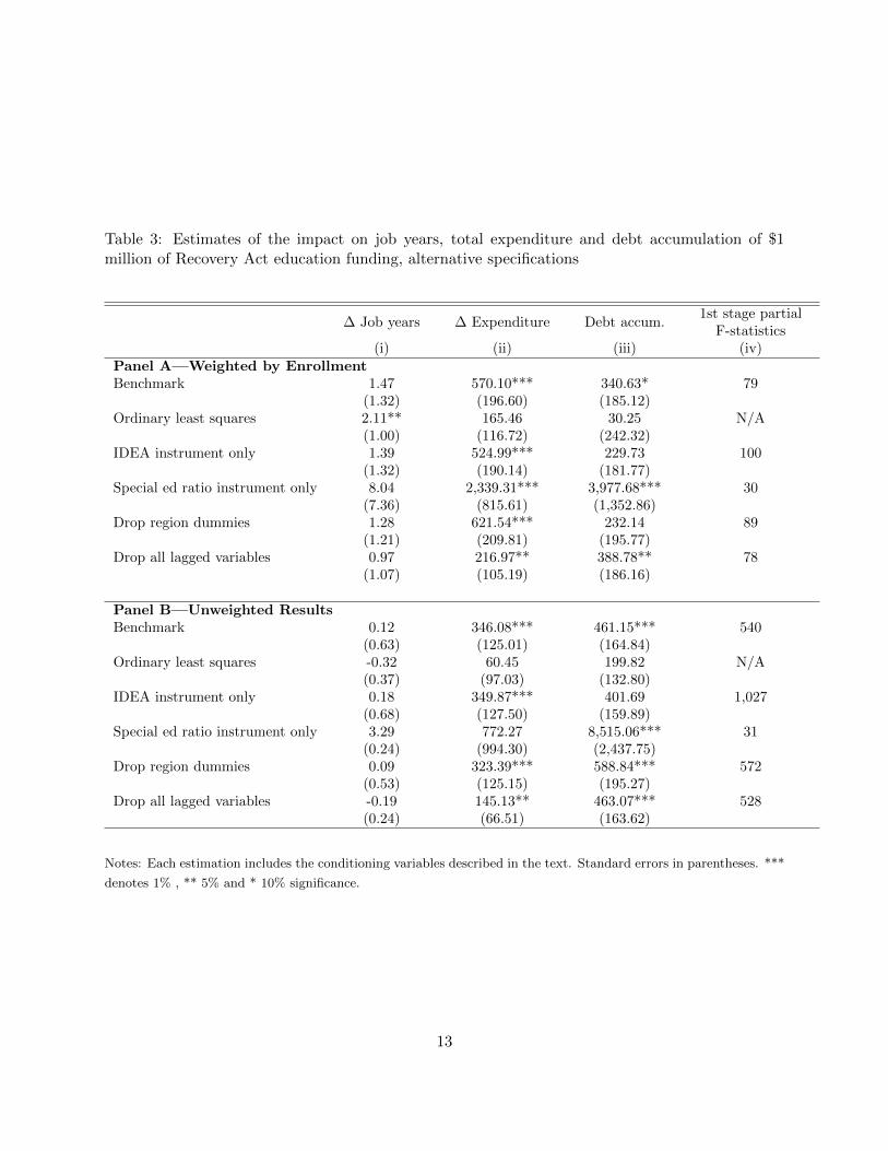
Table 3: Estimates of the impact on job years, total expenditure and debt accumulation of $1million of Recovery Act education funding, alternative specifications

∆ Job years

(i)

∆ Expenditure

(ii)

Debt accum.

(iii)

1st stage partialF-statistics

(iv)Panel A—Weighted by EnrollmentBenchmark 1.47 570.10*** 340.63* 79

(1.32) (196.60) (185.12)Ordinary least squares 2.11** 165.46 30.25 N/A

(1.00) (116.72) (242.32)IDEA instrument only 1.39 524.99*** 229.73 100

(1.32) (190.14) (181.77)Special ed ratio instrument only 8.04 2,339.31*** 3,977.68*** 30

(7.36) (815.61) (1,352.86)Drop region dummies 1.28 621.54*** 232.14 89

(1.21) (209.81) (195.77)Drop all lagged variables 0.97 216.97** 388.78** 78

(1.07) (105.19) (186.16)

Panel B—Unweighted ResultsBenchmark 0.12 346.08*** 461.15*** 540

(0.63) (125.01) (164.84)Ordinary least squares -0.32 60.45 199.82 N/A

(0.37) (97.03) (132.80)IDEA instrument only 0.18 349.87*** 401.69 1,027

(0.68) (127.50) (159.89)Special ed ratio instrument only 3.29 772.27 8,515.06*** 31

(0.24) (994.30) (2,437.75)Drop region dummies 0.09 323.39*** 588.84*** 572

(0.53) (125.15) (195.27)Drop all lagged variables -0.19 145.13** 463.07*** 528

(0.24) (66.51) (163.62)

Notes: Each estimation includes the conditioning variables described in the text. Standard errors in parentheses. ***

denotes 1% , ** 5% and * 10% significance.

13

Table 4: Estimates of the impact on staff employment of $1 million of Recovery Act educationgrants, by job type

∆ Teacher-JY ∆ Non Teacher-JY(i) (ii)

Recovery Act education -0.03 1.50spending per pupil (0.51) (0.99)Full Controls Yes YesNo. of Observations 6786 6786Partial F-stat 78.93 78.93

Notes: Each estimation includes the benchmark conditioning variables described in the text. The regressions are

enrollment weighted. Standard errors in parentheses. *** denotes 1% , ** 5% and * 10% significance.

Table 5: Estimates of the impact on expenditure of $1 million of Recovery Act education funding,by major expenditure categories

∆ Expenditure ∆ Capital ∆ Salaries ∆ Benefits(i) (ii) (iii) (iv)

Recovery Act education 570.10*** 390.82*** 8.92 79.38*spending per pupil (196.60) (149.34) (41.23) (48.00)Full Controls Yes Yes Yes YesNo. of Observations 6786 6786 6786 6786Partial F-stat 78.93 78.93 78.93 78.93

Notes: Each estimation includes the conditioning variables described in the text. The regressions are enrollment

weighted. Standard errors in parentheses. *** denotes 1% , ** 5% and * 10% significance. Expenditures and debt

accumulation variables are in units of thousands of dollars.

specification, except we estimate the equation separately for the change in the number of teaching

and non-teaching employees.

Column (i) of Table 4 shows that there was no statistically significant effect on the number of

teacher jobs created/saved. The point estimate equals -0.03 (SE = 0.51). District administrators

may have sought, as a top priority, to maintain class sizes at their pre-recession levels. This

constancy may have been achieved by neither hiring nor firing teachers on net.

The employment effect came through non-teacher jobs. As seen in column (ii), each $1 million

resulted in 1.50 (SE = 0.99) additional job-years of non-teacher employment, although this too is

not statistically different from zero.

Next, Table 5 examines the categories of spending that account for most of the effect on total

expenditures. In columns (ii) through (iv), we estimate the benchmark model except we in turn

replace the change in total expenditures with the change in a component of total expenditures.

Column (ii) shows that there is a substantial effect on capital outlays of Recovery Act aid.

14

Roughly 70% of all expenditures came in the form of capital outlays.19 Why might districts have

used so much of their grant money for investments? First, suppose a district seeks to maximize its

provision of education services as well as keep those provided services relatively smooth over time,

in a similar manner as the permanent income model of consumption smoothing. Second, suppose

education services are a function of labor, i.e. the number of staff, and capital. In this case, a

district that receives a one-time grant may seek to spread the benefits of this grant over many

periods by using a part of its grant to increase its capital stock.

Likewise, a district that received a relatively small amount of aid may have found that the best

way to close budget gaps was to temporarily cut back on investment in capital rather than layoff

staff. Because the capital stock depreciates slowly, a temporary interruption in investment would

likely have only a small effect on the quality of education services that the school could provide.

Recall that earlier in the paper, we document that Recovery Act aid tended to increase debt

accumulation. This effect may be related to the positive effect of aid on capital expenditure seen in

Table 5. Suppose that, upon receipt of Recovery Act funds, a district decided to spend part of its

funds on capital, such as construction. The district may have chosen to boost the dollars available

for construction by leveraging up the grant aid via borrowing. Under this scenario, had the district

attempted to finance the entire capital project with only debt, it may have been unable to secure

the funds or else be offered a reasonable financing rate. Thus, it is possible that grants may have

led to borrowing rather than saving by some districts.

Note that the construction spending itself is likely to have a positive jobs effect because of

building contractors the district might hire. These numbers are not reflected in our employment

estimate because we restrict attention to school district employees.20

Column (iii) of Table 5 reports the impact of aid on salaries, which was small and not statistically

different from zero.21 Since the employment effect was so small, it is not surprising that we do not

recover a substantial wage effect. Column (iv) of Table 5 implies that $1 million in aid increased

benefits paid by the school district by $79 million.

4 A model of school district hiring and capital decisions

In this section, we study the dynamic optimization problem of a school district facing stochastic

revenue shocks.

In the previous section, we found that the ratio of stimulus spending for paying education

workers relative to capital investment was 0.25. This may be puzzling since, as we explain below,

19Capital outlays include construction and purchases of equipment, land and existing structures.20Dupor and McCrory (2015) conduct a cross-regional analysis of the Recovery Act in a more broader context

than only education. That paper examines employment from all sectors and the act’s entire spending component, incontrast to that solely from education. They find a larger jobs effect than that estimated in the current paper.

21The salary and benefits variables are constructed in the equivalent manner as the variable for total expenditureswas constructed.

15

the long run average of this ratio equals 8. Second, there was a small effect on non-teacher staffing

and no effect on the number of teachers employed. Our model simulations will roughly match both

of these findings.

Moreover, our model allows us to estimate the medium and long-run effects of these grants and

provides a laboratory to study the effects of alternative hypothetical stimulus programs aimed at

schools.

4.1 The stylized facts

We begin by documenting two stylized facts about education spending by analyzing a 17 year panel

of district-level data ending with the 2011SY.22 The facts provide guidance for building and then

calibrating our economic model.

Our panel covers a long time span and some of our series contain time trends. As such, we

detrend every variable xt by its aggregate (over districts) gross growth rate between period t and

Q, the final period in our sample. The cumulative growth rate is:

cgx,t =

∑i∈I xi,t∑i∈I xi,Q

where I is the set of all districts. The detrended district level variable is then xt is thus

xi,t =xi,tcgx,t

Unless otherwise noted, each variable is scaled by its district enrollment.

Stylized Fact 1: The teacher to student ratio is less volatile than the non-teacher to student ratio.

For each district i, we compute the time series variance of the log deviation of the employment

levels of teachers, T , and non-teaching workers, N .23

vx,i = variance across t of log

[xi,t

1Q

∑t xi,t

]for x ∈ (T,N).

Columns (i) and (ii) of Table 6 contain the across-district median value (along with the 10th,

25th, 75th, and 90th percentile values) of vT,i and vN,i. Observe that the non-teacher/student ratio

is more variable than the teacher/student ratio. The difference in variability ranges from 3 times

as high for the 10th percentile, 4 times as high for the median, and over 5 times as high for the

22We use the merged Universe and Finance surveys of the Common Core School District data set. The 1994SYis the first year for which the entire data set is available. As in the paper’s previous section, we drop districts thatreport less than 500 students.

23Non-teacher staff includes instructional aides, guidance counselors, library/media staff, administrative supportstaff, etc.

16

90th percentile.

As further robustness, columns (iii)-(iv) contain the statistics for a smaller subsample that

includes data from the most recent 6 years. Whereas the shorter time horizon results in a reduced

value of the magnitude of the variance, as in the full sample in this subsample, the teacher/student

ratio remains less variable than the non-teacher/student ratio.

Table 6: Volatility of the Teacher/Student & Non-Teacher/Student Ratio

Time-Series Variance of Log Deviations fromthe Aggregate Trend of the Per Student Ratio

(i) (ii) (iii) (iv)Teacher Non-Teacher Teacher Non-Teacher

10th Perc 0.0012 0.0036 0.0004 0.000825th Perc 0.0018 0.0062 0.0007 0.0017Median 0.0033 0.0122 0.0016 0.003875th Perc 0.0062 0.0245 0.0039 0.009390th Perc 0.0104 0.0555 0.0092 0.0232

Years 1994-2011 2006-2011Number of districts 1901 4291

Stylized Fact 2: Capital spending is more volatile than that of labor.

Next, we consider the behavior of two categories of spending: capital expenditure and labor

expenditure. Capital expenditure is the sum of spending on construction, land and existing struc-

tures, and equipment with an expected life of 5 or more years. Labor expenditures includes salaries

and benefits of district employees.24 We convert each variable into real terms using the GDP

deflator with a base year of 2011.

Table 7 reports the across-district median value (along with the 10th, 25th, 75th, and 90th

percentile values) of the time-series volatility of expenditures on total real salary plus benefits

and real capital outlays, where each volatility is calculated as the time-series variance of the log

deviations of the variable from its aggregate trend using (4.1). Note that investment is significantly

more variable than labor expenditures. At the median level of variability, expenditure on capital

is 250 times more variable than expenditures on labor.

Next, we break the capital category into spending of two types: construction, land, and existing

structures (CLS) and equipment. Table 8 reports the volatility of these variables. Even though

equipment itself is volatile, most of the volatility in capital is driven by CLS. This fact coupled with

the facts that CLS makes up roughly 80% of all capital investment and that labor expenditure is

24We exclude services and non-durable good expenditures in our descriptions here. In regression results notprovided in the paper (but available on request), we establish that there was a negligible effect of grants on thesetypes of spending. We also exclude debt service payments, payments to other districts and expenditures on non-elementary/secondary programs because they make up only 10% of the average district’s spending and our outsideof our model.

17

Table 7: Volatility of Pay/Student and Capital/Student ratios

Time-Series Variance of Log Deviations from theAggregate Trend of the Per Student Ratio

(i) (ii)Salary + Benefits All Capital Outlays

10th Perc 0.0013 0.333925th Perc 0.0021 0.5860Median 0.0036 0.958075th Perc 0.0064 1.472090th Perc 0.01113 2.0509

Dates 1994-2010Number of districts 6092

Table 8: Volatility of the (Salary + Benefits)/Student and the Investment/Student ratios

Time-Series Variance of Log Deviations from theAggregate Trend of the Per Student Ratio

(i) (ii) (iii)Constr./Land/Struc. Equipment All Capital Outlays

10th Perc 0.5657 0.1141 0.333925th Perc 1.0089 0.1861 0.5860Median 1.7008 0.3255 0.958075th Perc 2.6626 0.5898 1.472090th Perc 3.9451 1.1045 2.0509

Dates 1994-2010Number of districts 6092

not very volatile pushes us towards a theory in which districts tend to use large revenue gains and

make-up for revenue shortfalls by largely either investing in, or delaying expenditure on, long lived

capital goods.

4.2 The economic model

Consider a school district that uses an exogenous stream of revenue, R, to hire workers and buy

capital to provide education services to its students. Its revenue process is given by the following

AR(1) process:

R′ = ρR+ (1− ρ)R+ εR with εR ∼ N (0, σR) (4.1)

where ρ ∈ (0, 1) and R is fixed. Revenue, as well as other variables in the model, are per pupil.

18

A district’s one-period welfare function is

W (T,N,K) = αU (T ; ξT ) + γU (N ; ξN ) + ηU (K; ξK) (4.2)

where T, N, and K are the number of teachers, number of non-teachers, and quantity of capital,

respectively. Moreover, let U (X; ξ) = X1−ξ/ (1− ξ).The district’s dynamic optimization problem is given by the following recursive functional equa-

tion:

V (K;R) = maxT,N,I

{W (T,N,K) + βE

[V (K ′;R′)|R

]}subject to

R = wTT + wNN + I (4.3)

K ′ = (1− δ)K + I (4.4)

and non-negativity constraints on T,N and K. Also, I represents investment in the capital good

and values with a prime subscript give the next period realization of that variable. For example,

K ′ gives the next period realization of capital, K.

Next, (4.3) is the district budget constraint, with wT and wN representing the teacher wage

and non-teacher wage, respectively. Also, (4.4) is the capital law of motion and δ is the capital

depreciation rate.

Every period the school district receives revenue which it optimally allocates to the hiring of

teacher and non-teachers, and capital acquisition. Whereas the amount of teachers and non-teachers

hired effect only the current period’s welfare, the durable nature of capital results in it having a

multi-period effect. As we discuss in the next section, the dynamics that result from allowing the

district to choose a durable input are important for understanding why the 2009 Recovery Act had

a small effect on hiring, but a large effect on capital outlays.

4.3 Calibration and simulations

The parameter values for the model are given in Table 9. The model period is equal to 1 year. We

begin our calibration by setting the discount factor β = 0.96 to match a 4% annual real interest

rate.

Next, in the data, the capital stock is comprised of two different basic types: equipment with

more than a 5 year lifespan and CLS. CLS account for roughly 75% of the capital outlays and de-

preciate at a 1.88% annual rate, while equipment accounts for 25% of capital outlays and depreciate

at a 15% annual rate.25 As such, we set the δ = 0.0516 (= 0.75× 0.0133 + 0.25× 0.16).

25See BEA Depreciation Estimates at http://www.bea.gov/national/FA2004/Tablecandtext.pdf

19

Across districts, the median wage bill per student is $8128, for which 48% go towards teacher

pay and 52% go towards non-teaching staff pay. Teacher compensation per pupil is thus $3901 and

non-teaching staff compensation equals $4227. The median teacher-student ratio is 1/15.5 and the

median number of non-teachers staff per student is 1/16. As a result we set teacher and non-teacher

wage wT = $60472 (= 15.5× 3901) and wN = $67625 (= 16× 4227).

The persistence of the AR(1) revenue process is directly estimated from the data. The median

auto-correlation of expenditures is 0.47. The average revenue is set at R = $8128 + $988 = $9116.

Six parameters remain: The welfare elasticities (ξT , ξN and ξK), the relative shares of teachers,

α, and non-teachers, γ, and the standard deviation of the revenue process, σR.

First, we set ξK = 1 and then jointly calibrate the remaining five parameters to match the

following five targets: The average teacher/student ratio is 0.064; the average non-teacher/student

ratio is 0.062; the non-teacher/student ratio is 4 times as volatile as the teacher/student ratio; the

average salary volatility equals 0.0036; and the average investment volatility 0.95.

Table 9: Parameter Values

Parameter Value Description Explanation

β 0.96 Discount factor Standard value for annual discount factor

δ 0.0516 Depreciation RateCalculated using the BEA data on the depreciation ofbuildings and equipment.

wT $60472 Wage rate for teachers Set equal to average teacher wage in the data.wN $67625 Wage rate for non-teachers Set equal to average non-teacher wage in the data.

R $9116 Average revenue per student Sum of average revenue on labor + capital.

ρ 0.47 Persistence of revenue processSet equal to the auto-correlation of district-levelexpenditure in the data.

ξK 1.0 Welfare elasticity of capital Normalized to 1

ξT 1.52 Welfare elasticity of teachers Jointly calibrated to match: (1) Avg. teacher/studentξN 0.76 Welfare elasticity of non-Teacher = 0.064, (2) Average non-teacher/student = 0.062 (3)α 0.086 Welfare share for teachers teacher/student 4x more volatile than non-teacherγ 0.751 Welfare share for non-teaching staff /student (4) Volatility of total salary = 0.0036,σR 1150 Std. Dev. of shock to revenue (5) Avg. volatility of investment = 0.95

4.4 The effect of a Recovery Act size shock

To simulate the effects of the Recovery Act, we alter equation (4.3) to be:

R+A = wTT + wNN + I (4.5)

where A gives the net magnitude of the Recovery Act shock to revenue after accounting for any loss

in revenue at the district level. From our benchmark regression analysis in Table 2, we estimate

the size of this shock to be $570 per student. As a result, we set A = $570 in the period of the

shock and A = $0 otherwise. For a transparent comparison with our regression results, all of our

20

results below are for a $1 million shock. In the data, the gross magnitude of the Recovery Act

shock before accounting for any loss in revenue at the district level was approximately $1000 per

student. As a result, to find the $1 million response we multiply the per student values by 1000.

Figure 1 plots the effect of the spending shock. The left-side panels give the per period impulse

responses and the right-side panels give the cumulative responses. As seen in the figure, over the

first two years the additional revenue creates 1.4 non-teaching staff jobs, 0.7 teaching jobs, and

increased investment by $435,000 for each million dollars spent. Note that other than the size

of the shock the model was calibrated independently of the regression results. Consequently, the

consistency between our regression results and the dynamic model give further evidence for a small

effect of the Recovery Act on employment.

The large effect on investment is driven by a motive to smooth the value of education inputs over

time. For the purpose of intuition, suppose a school district had two mutually exclusive uses of new

funds: (1) increasing the number of staff for one year, or (2) engaging in additional investment for

one year. The latter option leads to more capital in the short and intermediate run which increases

education services. Also, since the capital is now higher, the district can cut back marginally on

investment in periods after the shock and use the funds saved to increase its staffing levels. The

latter option leads to an increased and smoother path of inputs over time, as well as higher welfare.

To illustrate this effect, Figure 1 plots plot the responses of the district in an calibration where

δ = 1.0, i.e. capital depreciates fully after one period. As seen in the figure, once the district loses

access to interperiod savings, the employment effect rises.

Note that our environment does not permit the district to smooth the benefit of the revenue

shock over time using savings or similarly deficit reduction. If we extended the model to permit

these options, districts would use these financial instruments as well as capital accumulation in an

optimal policy. Note, however, that our regression results instead find that deficits increased upon

receipt of Recovery Act grants. As explained earlier, the deficit results may be a result of districts

pairing new capital spending with increased leverage through higher debt levels.

Next, one of our stylized facts was that the volatility of the number of teachers is significantly

lower than that of non-teachers. We conjecture that this occurs because there may be little flexibility

in hiring or laying off teachers. Consider a school that teaches five subjects - math, English, Spanish,

social studies, and science - to 80 students and currently hires one teacher for each subject. This

school may be unable to lay off a teacher because doing so would lead to one fewer subject being

taught. If it wanted to add one teacher, the additional teacher could not teach a bit of all five

subjects. Thus, the marginal benefit of hiring one extra, say math, teacher is very low. On the other

hand, hiring non-teaching staff across the district likely would not face a classroom indivisibilty

constraints. The relatively low volatility of teacher employment can be achieved in the model with

a high value of ξT relative to ξN . Thus ξT > ξN proxies for a relatively low flexibility in changing

21

02

46

810

−20246x

105

Investment/StudentIn

vest

men

t

Bas

elin

eF

ull

Dep

reci

atio

nξ T

= ξ

N =

1 a

nd

α =

γ =

0.4

202

46

810

0246x

105

Investment/Student

Inve

stm

ent

− C

um

ula

tive

Eff

ect

02

46

810

−10123

Teachers/Student

Tea

cher

s

02

46

810

01234 Teachers/Student

Tea

cher

s −

Cu

mu

lati

ve E

ffec

t

02

46

810

−20246

Non−Teachers/Student

Yea

rs

No

n−T

each

ing

Sta

ff

02

46

810

0246 Non−Teachers/StudentY

ears

No

n−T

each

ing

Sta

ff −

Cu

mu

lati

ve E

ffec

t

Fig

ure

1:Im

pu

lse

Res

pon

ses

toa

Rec

over

yA

ctsi

zesh

ock

22

the teaching staff level. Figure 1 plots impulse responses if ξT = ξN .26 When the elasticities for

teachers and non-teachers are identical the response between them is are more closely aligned.

Our model also permits us to estimate the shock’s long-run effects. As discussed above, the

initial effect of the shock is driven largely by an education-services smoothing motive which results

in accumulating capital initially. This, in turn, frees up future resources for hiring teachers and

non-teachers. As seen in Figure 1, the cummulative ten year effect is approximately two teachers

and four non-teachers per million dollars spent. Note that these effect are larger than the two year

effect. The long run effect still dwarfs the CEA’s estimate that over 750,000 education jobs were

created/saved by the act. At 2.25 jobs per $1 million in 2 years and 6 jobs per million in 10 years,

the $64.7 billion spent by the Department of Education creates 146,000 jobs in the first two years

and 388,000 jobs in the first ten years following the act’s passage.

Policy Analysis

Our model provides a laboratory to study the effects of alternative ways to implement a stimulus

program. First, a simple, and it turns out simplistic, policy would require all districts to use stimulus

money on employment only, i.e.

A ≤ wTT + wNN (4.6)

Figure 2 plots the response to this policy. The policy has no effect, relative to the “no constraint”

case presented above. This is because a district’s existing revenue and the stimulus money are

fungible. In response to a stimulus shock, a district can cut back on using its existing revenue

to pay labor and instead use the stimulus money to hire workers. The district would meet the

requirement of using stimulus money to hire workers and maintain the no constraint outcome.

Consider an alternative policy where, instead, the federal government requires that in the period

of the shock:

φ(R+A) ≤ wTT + wNN (4.7)

where φ gives the percentage of the all revenue that must be used to pay workers. We simulate

the model under this policy, setting φ = 0.875, which we find achieves the maximum employment

effect (while keeping investment constant). Figure 3 gives the results of this exercise. This has a

significantly larger response of 9 new jobs (3 teaching + 6 non-teaching) in the year of the shock.

Our model also allows us to consider much richer policy alternatives where the percentage of

revenue depends on the amount of revenue and capital at the district level. For figure 4 we first

calculate the pre-stimulus response of the district and then require that the district use all its

stimulus revenue plus all revenue it would have used toward hiring labor had it not gotten the

stimulus revenue. The figure then plots what percentage of the total post-stimulus revenue this

26The value of α and γ are jointly determined with ξT and ξN .

23

02

46

810

−20246x

105

Investment/StudentIn

vest

men

t

Bas

elin

eP

olic

y: U

se a

ll A

RR

A M

on

ey o

n L

abo

r

02

46

810

0246x

105

Investment/Student

Inve

stm

ent

− C

um

ula

tive

Eff

ect

02

46

810

0

0.1

0.2

0.3

0.4

Teachers/Student

Tea

cher

s

02

46

810

0123 Teachers/Student

Tea

cher

s −

Cu

mu

lati

ve E

ffec

t

02

46

810

0

0.2

0.4

0.6

0.8

Non−Teachers/Student

Yea

rs

No

n−T

each

ing

Sta

ff

02

46

810

01234 Non−Teachers/StudentY

ears

No

n−T

each

ing

Sta

ff −

Cu

mu

lati

ve E

ffec

t

Fig

ure

2:Im

pu

lse

Res

pon

ses

toa

Rec

over

yA

ctsi

zesh

ock

24

02

46

810

−20246x

105

Investment/StudentIn

vest

men

t

Bas

elin

eP

olic

y: U

se 8

7.5%

of

Rev

enu

e o

n L

abo

r

02

46

810

−20246x

105

Investment/Student

Inve

stm

ent

− C

um

ula

tive

Eff

ect

02

46

810

0123 Teachers/Student

Tea

cher

s

02

46

810

0123 Teachers/Student

Tea

cher

s −

Cu

mu

lati

ve E

ffec

t

02

46

810

0246 Non−Teachers/Student

Yea

rs

No

n−T

each

ing

Sta

ff

02

46

810

02468 Non−Teachers/StudentY

ears

No

n−T

each

ing

Sta

ff −

Cu

mu

lati

ve E

ffec

t

Fig

ure

3:Im

pu

lse

Res

pon

ses

toa

Rec

over

yA

ctsi

zesh

ock

25

amount would have been.

As seen in the figure, as an optimal policy, the government should impose a larger percentage

of revenue used on labor for districts with lower revenues and high levels of capital. Districts with

lower levels of revenue in particular are motivated to use the additional stimulus revenue they

receive from the government on capital.

5 Conclusion

This paper explores the impact of countercyclical government spending on the education sector.

Empirically, we find that the Recovery Act’s education component had a small impact on non-

teacher employment, no effect on teacher staff levels, and a substantially less than one-for-one

response of district level expenditures. To the extent that government grants increased district

expenditures, the increases largely took the form of capital outlays. The grants also stimulated

district debt accumulation.

These findings should not be entirely surprising given the decentralized nature of the act’s

implementation plan. The allocation process was multi-tiered, with local and state governments

having latitude regarding how Recovery Act dollars were spent. First, state governments maintained

substantial control over how they spent their own revenue. This created an environment where

stimulus dollars might be used to replace state contributions.27

After passing through the state-level, the Recovery Act dollars were spent by individual districts

largely at their own discretion. Given that the stimulus dollars were temporary, districts had

incentive to smooth out the spike in additional education services that they could provide by

investing in equipment and structures. This objective is one potential explanation for the small

education jobs effect that we estimate in this paper.

27As Inman (2010) writes, “States are important ‘agents’ for federal macro-policy, but agents with their own needsand objectives.”

26

Fig

ure

4:O

pti

mal

Pol

icy

27

References

American Association of School Administrators (2012), “Weathering the Storm: How the Economic

Recession Continues to Impact School Districts,” March.

Biden, J. (2011), “Roadmap to Recovery,” extracted from www.whitehouse.gov.

Bradford, D. and W. Oates (1971), “The Analysis of Revenue Sharing in a New Approach to

Collective Fiscal Decisions,” Quarterly Journal of Economics 85, pp. 416-439.

Cavanaugh, S. (2011), “Education Regroups in Recession’s Aftermath,” Education Week.

Chakrabarti, R. and E. Setren (2011), “The Impact of the Great Recession on School District

Finances: Evidence from New York,” Federal Reserve Bank of New York Working Paper.

Chodorow-Reich, G., L. Feiveson, Z. Liscow and W. Woolston (2012), “Does State Fiscal Relief

During Recessions Increase Employment? Evidence from the American Recovery and Reinvest-

ment Act,” American Economic Journal: Economic Policy.

Congressional Budget Office (various quarterly reports), “Estimated Impact of the American Re-

covery and Reinvestment Act on Employment and Economic Output.”

Conley, T. and B. Dupor (2013), “The American Recovery and Reinvestment Act: Solely a Gov-

ernment Jobs Program?” Journal of Monetary Economics, 60, 535-549.

Council of Economic Advisers (various quarterly reports), “The Economic Impact of the American

Recovery and Reinvestment Act of 2009.”

Dinerstein, M., C. Hoxby, J. Meyer and P. Villanueva (2013), “Did the Fiscal Stimulus Work for

Universities.”

Dupor, B. (2014), “The 2009 Recovery Act: Directly Created and Saved Jobs Were Primarily in

Government,” Federal Reserve Bank of St. Louis Review, Second Quarter, 96(2), 123-145.

Dupor, B. and P. McCrory (2015), “A Cup Runneth Over: Fiscal Policy Spillovers from the 2009

Recovery Act,” Federal Reserve Bank of St. Louis.

Education, U.S. Dept. of (2009a), “Guidance on the State Fiscal Stabilization Fund Program,”

April.

Education, U.S. Dept. of (2009b), “Guidance: Funds for Part B of the Individuals with Disabilities

Act Made Available under the American Recovery and Reinvestment Act of 2009,” July 1,

revised.

28

Education, U.S. Dept. of Education (2009c), “Memorandum: The American Recovery and Rein-

vestment Act of 2009 Individuals with Disabilities Education Act Part B Grants to States and

Preschool Grants,” Office of Special Education and Rehabilitative Services, April 1, (including

Enclosures A, B and C).

Evans, W. and E. Owens (2007), “COPS and Crime,” Journal of Public Economics 91, pp. 181-201.

Executive Office of the President of the United States (2009), “Educational Impact of the Amer-

ican Recovery and Reinvestment Act,” Domestic Policy Council in Cooperation with the U.S.

Department of Education, October.

Feyrer, J. and B. Sacerdote (2012), “Did the Stimulus Stimulate? Effects of the American Recovery

and Reinvestment Act,” Dartmoth College.

Gordon, N. (2004), “Do Federal Grants Boost School Spending? Evidence from Title I,” Journal

of Public Economics 88, pp. 1771-1792.

Gramlich, E. (1979), “Stimulating the Macroeconomy through State and Local Governments,”

American Economic Review 68(2), 180-185.

Inman, Robert (2010), “States in Fiscal Distress,” NBER Working Paper 16086.

Leduc, S. and D. Wilson (2013), “Are State Governments Roadblocks to Federal Stimulus? Evi-

dence from Highway Grants in the 2009 Recovery Act,” Federal Reserve Bank of San Fransisco.

Lundqvist, H., M. Dahlberg and E. Mork (2014), “Stimulating Local Government Employment:

Do General Grants Work?,” American Economic Journal: Economic Policy, pp. 167-192.

New America Foundation (2014), “Individuals with Disabilities Education Act-Funding Distribu-

tion,” Federal Education Budget Project, April.

Recovery Accountability and Transparency Board (2009), “Recovery.gov: Download Center Users

Guide,” Recovery.gov.

Wilson, D. (2012), “Fiscal Spending Jobs Multipliers: Evidence from the 2009 American Recovery

and Reinvestment Act,” American Economic Journal: Economic Policy.

29

Appendix

Table A.1: Number of jobs directly created and saved through grants, contracts and loans admin-istered by the U.S. Department of Education, first two school years following enactment

Quarter Education jobs

2009Q3 397,982.432009Q4 423,616.332010Q1 470,197.342010Q2 454,281.082010Q3 344,308.142010Q4 309,187.212011Q1 319,494.262011Q2 307,901.15

Total 756,741.99(Annualized)

Notes: Jobs are measured in units of full-time equivalents. Source is Recovery.gov.

30