The International Journal of Parallel, Emergent and Distributed SystemsVol. 00, No. 00, Month 2011, 1–22

RESEARCH ARTICLE

Simple Memory Machine Models for GPUs

Koji Nakanoa∗

aDepartment of Information Engineering, Hiroshima University

Kagamiyama 1-4-1, Higashi Hiroshima, 739-8527 Japan(Received 00 Month 200x; in final form 00 Month 200x)

The main contribution of this paper is to introduce two parallel memory machines, the DiscreteMemory Machine (DMM) and the Unified Memory Machine (UMM). Unlike well studiedtheoretical parallel computational models such as PRAMs, these parallel memory machinesare practical and capture the essential feature of GPU memory accesses. As a first step ofthe development of algorithmic techniques on the DMM and the UMM, we first evaluatethe computing time for the contiguous access and the stride access to the memory on thesemodels. We then go on to present parallel algorithms to transpose a 2-dimensional array onthese models and evaluate their performance. Finally, we show that, for any permutationgiven in off-line, data in an array can be moved efficiently along the given permutation bothon the DMM and on the UMM. Since the computing time of our permutation algorithms onthe DMM and the UMM is equal to the sum of the lower bounds obtained from the memorybandwidth limitation and the latency limitation, they are optimal from the theoretical pointof view. We believe that the DMM and the UMM can be good theoretical platforms to developalgorithmic techniques for GPUs.

Keywords: Memory banks, Parallel computing models, Parallel algorithms, Matrixtranspose, Array permutation, GPU, CUDA

1. Introduction

1.1 Background

The research of parallel algorithms has a long history of more than 40 years. Se-quential algorithms have been developed mostly on the Random Access Machine(RAM) [1]. In contrast, since there are a variety of connection methods and pat-terns between processors and memories, many parallel computing models have beenpresented and many parallel algorithmic techniques have been shown on them. Themost well-studied parallel computing model is the Parallel Random Access Machine(PRAM) [2–4], which consists of processors and a shared memory. Each processoron the PRAM can access any address of the shared memory in a time unit. ThePRAM is a good parallel computing model in the sense that parallelism of eachproblem can be revealed by the performance of parallel algorithms on the PRAM.However, since the PRAM requires a shared memory that can be accessed by allprocessors at the same time, it is imaginary and impractical.

The GPU (Graphical Processing Unit), is a specialized circuit designed to accel-erate computation for building and manipulating images [5–8]. Latest GPUs aredesigned for general purpose computing and can perform computation in applica-tions traditionally handled by the CPU. Hence, GPUs have recently attracted theattention of many application developers [5, 9, 10]. NVIDIA provides a parallel

∗Corresponding author. Email: nakano@cs.hiroshima-u.ac.jp

ISSN: 1744-5760 print/ISSN 1744-5779 onlinec© 2011 Taylor & FrancisDOI: 10.1080/17445760.YYYY.CATSidhttp://www.informaworld.com

2 Koji Nakano

computing architecture called CUDA (Compute Unified Device Architecture) [11],the computing engine for NVIDIA GPUs. CUDA gives developers access to the vir-tual instruction set and memory of the parallel computational elements in NVIDIAGPUs. In many cases, GPUs are more efficient than multicore processors [12], sincethey have hundreds of processor cores and very high memory bandwidth.

CUDA uses two types of memories in the NVIDIA GPUs: the shared memory andthe global memory [11]. The shared memory is an extremely fast on-chip memorywith lower capacity, say, 16-64 Kbytes. The global memory is implemented as anoff-chip DRAM, and has large capacity, say, 1.5-6 Gbytes, but its access latency isvery long. The efficient usage of the shared memory and the global memory is a keyfor CUDA developers to accelerate applications using GPUs. In particular, we needto consider the bank conflict of the shared memory access and the coalescing of theglobal memory access [6, 12, 13]. The address space of the shared memory is mappedinto several physical memory banks. If two or more threads access the same memorybanks at the same time, the access requests are processed sequentially. Hence, tomaximize the memory access performance, threads of CUDA should access distinctmemory banks to avoid the bank conflicts of the memory accesses. To maximizethe bandwidth between the GPU and the DRAM chips, the consecutive addressesof the global memory must be accessed at the same time. Thus, CUDA threadsshould perform coalesced access when they access the global memory.

There are several previously published works that aim to present theoreticalpractical parallel computing models capturing the essence of parallel computers.Many researchers have been devoted to developing efficient parallel algorithms tofind algorithmic techniques on such parallel computing models. For example, pro-cessors connected by interconnection networks such as hypercubes, meshes, trees,among others [14], bulk synchronous models [15], LogP models [16], reconfigurablemodels [17], among others. As far as we know, no sophisticated and simple parallelcomputing model for GPUs has been presented. Since GPUs are attractive paral-lel computing devices for many developers, it is challenging work to introduce atheoretical parallel computing model for GPUs.

1.2 Our Contribution: Introduction to the Discrete Memory Machine and

the Unified Memory Machine

The first contribution of this paper is to introduce simple parallel memory machinemodels that capture the essential features of the bank conflict of the shared mem-ory access and the coalescing of the global memory access. More specifically, wepresent two models, the Discrete Memory Machine (DMM) and the Unified Mem-ory Machine (UMM), which reflect the essential features of the shared memoryand the global memory of NVIDIA GPUs.

The outline of the architectures off the DMM and the UMM are illustrated inFigure 1. In both architectures, a sea of threads (Ts) are connected to the memorybanks (MBs) through the memory management unit (MMU). Each thread is aRandom Access Machine (RAM) [1], which can execute fundamental operationsin a time unit. We do not discuss the architecture of the sea of threads in thispaper, but we can imagine that it consists of a set of multi-core processors whichcan execute many threads in parallel. Threads are executed in SIMD [18] fashion,and the processors run on the same program and work on the different data. Inprinciple, each thread is assigned a local memory (or local registers) that canaccess O(1) words of data. However, sometimes, we assume that each thread hasmore than O(1) local registers, if many registers are very useful to accelerate thecomputation. If this is the case, we assume that each thread has r local registers

Simple Memory Machine Models for GPUs 3

to store words of data. In either cases, we assume that each thread can access alocal register in 1 time unit.

DMM UMM

MMU

MB MB MB MB

MMU

MB MB MB MB

T T T T T T

T T T T T T

T T T T T T

T T T T T T

T T T T T T

T T T T T T

T T T T T T

T T T T T T

a sea of threads a sea of threads

data lineaddress line

T: Thread, MMU:Memory Management Unit, MB: Memory Bank

Figure 1. The architectures of the DMM and the UMM

MBs constitute a single address space of the memory. A single address space ofthe memory is mapped to the MBs in an interleaved way such that the word ofdata of address i is stored in the (i mod w)-th bank, where w is the number ofMBs. The main difference of the two architectures is the connection of the addressline between the MMU and the MBs, which can transfer an address value. In theDMM, the address lines connect the MBs and the MMU separately, while a singleaddress line from the MMU is connected to the MBs in the UMM. Hence, in theUMM, the same address value is broadcast to every MB, and the same address ofthe MBs can be accessed in each time unit. On the other hand, different addressesof the MBs can be accessed in the DMM. Since the memory access of the UMM ismore restricted than that of the DMM, the UMM is less powerful than the DMM.

The performance of algorithms on the PRAM is usually evaluated using twoparameters: the size n of the input and the number p of processors. For example,it is well known that the sum of n numbers can be computed in O(n

p + log p) time

on the PRAM [2]. We will use four parameters, the size n of the input, the numberp of threads, the width w and the latency l of the memory when we evaluatethe performance of algorithms on the DMM and on the UMM. The width w is thenumber of memory banks and the latency l is the number of time units to completethe memory access. Hence, the performance of algorithms on the DMM and theUMM is evaluated as a function of n (the size of a problem), p (the number ofthreads), w (the width of a memory), and l (the latency of a memory). Further, r(the number of local registers used by each thread) may be additionally used.

In NVIDIA GPUs, the width w of the shared memory and the global memoryis 16 or 32. Also, the latency l of the global memory is several hundreds clockcycles. In CUDA, a grid can have at most 65535 blocks with at most 1024 threadseach [11]. Thus, the number p of threads can be 65 million.

1.3 Position and Role of Memory Machine Models, the DMM and the

UMM

The DMM and the UMM are theoretical models of parallel computation, thatcapture the essential feature of the shared memory and the global memory of GPUs.The architecture of the GPUs are more complicated. It is a hybrid of the DMM

4 Koji Nakano

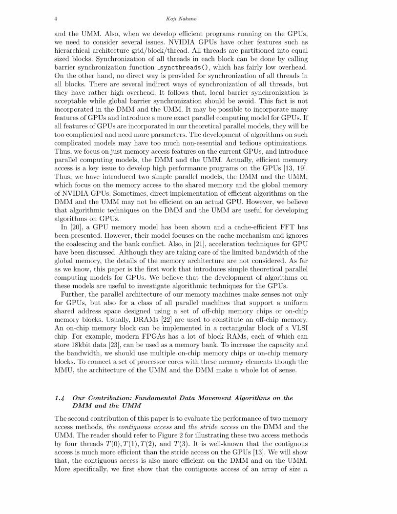
and the UMM. Also, when we develop efficient programs running on the GPUs,we need to consider several issues. NVIDIA GPUs have other features such ashierarchical architecture grid/block/thread. All threads are partitioned into equalsized blocks. Synchronization of all threads in each block can be done by callingbarrier synchronization function syncthreads(), which has fairly low overhead.On the other hand, no direct way is provided for synchronization of all threads inall blocks. There are several indirect ways of synchronization of all threads, butthey have rather high overhead. It follows that, local barrier synchronization isacceptable while global barrier synchronization should be avoid. This fact is notincorporated in the DMM and the UMM. It may be possible to incorporate manyfeatures of GPUs and introduce a more exact parallel computing model for GPUs. Ifall features of GPUs are incorporated in our theoretical parallel models, they will betoo complicated and need more parameters. The development of algorithms on suchcomplicated models may have too much non-essential and tedious optimizations.Thus, we focus on just memory access features on the current GPUs, and introduceparallel computing models, the DMM and the UMM. Actually, efficient memoryaccess is a key issue to develop high performance programs on the GPUs [13, 19].Thus, we have introduced two simple parallel models, the DMM and the UMM,which focus on the memory access to the shared memory and the global memoryof NVIDIA GPUs. Sometimes, direct implementation of efficient algorithms on theDMM and the UMM may not be efficient on an actual GPU. However, we believethat algorithmic techniques on the DMM and the UMM are useful for developingalgorithms on GPUs.

In [20], a GPU memory model has been shown and a cache-efficient FFT hasbeen presented. However, their model focuses on the cache mechanism and ignoresthe coalescing and the bank conflict. Also, in [21], acceleration techniques for GPUhave been discussed. Although they are taking care of the limited bandwidth of theglobal memory, the details of the memory architecture are not considered. As faras we know, this paper is the first work that introduces simple theoretical parallelcomputing models for GPUs. We believe that the development of algorithms onthese models are useful to investigate algorithmic techniques for the GPUs.

Further, the parallel architecture of our memory machines make senses not onlyfor GPUs, but also for a class of all parallel machines that support a uniformshared address space designed using a set of off-chip memory chips or on-chipmemory blocks. Usually, DRAMs [22] are used to constitute an off-chip memory.An on-chip memory block can be implemented in a rectangular block of a VLSIchip. For example, modern FPGAs has a lot of block RAMs, each of which canstore 18kbit data [23], can be used as a memory bank. To increase the capacity andthe bandwidth, we should use multiple on-chip memory chips or on-chip memoryblocks. To connect a set of processor cores with these memory elements though theMMU, the architecture of the UMM and the DMM make a whole lot of sense.

1.4 Our Contribution: Fundamental Data Movement Algorithms on the

DMM and the UMM

The second contribution of this paper is to evaluate the performance of two memoryaccess methods, the contiguous access and the stride access on the DMM and theUMM. The reader should refer to Figure 2 for illustrating these two access methodsby four threads T (0), T (1), T (2), and T (3). It is well-known that the contiguousaccess is much more efficient than the stride access on the GPUs [13]. We will showthat, the contiguous access is also more efficient on the DMM and on the UMM.More specifically, we first show that the contiguous access of an array of size n

Simple Memory Machine Models for GPUs 5

T (0)

T (1)

T (2)

T (3)

contiguous access stride access

0 1 2 3 4

5 6 7 8 9

10 11 12 13 14

15 16 17 18 19

0 1 2 3

4 5 6 7

8 9 10 11

12 13 14 15

16 17 18 19

T (0)T (1)T (2)T (3)

Figure 2. The contiguous access and the stride access for p = 4 and n = 16.

can be done in O( nw + nl

p ) time units on the DMM and the UMM. We also show

two lower bounds, Ω( nw ) time units by the bandwidth limitation and Ω(nl

p ) timeunits by the latency limitation to access all of data in an array of size n. Thus, thecontiguous access on the DMM and the UMM is optimal. Further, we will showthat the stride access on the DMM can be done in O( n

w · GCD(np , w) + nl

p ) time

units on the DMM, where GCD(np , w) is the greatest common divisor of n

p and

w. Hence, the stride access on the DMM is optimal if np and w are co-prime. The

stride access on the UMM can be done in O(min(n, nw · n

p + nlp )) time units. Hence,

the stride access on the UMM needs an overhead of a factor of np .

From these memory access results, we have one important observation as follows.The factor n

w in the computing time comes from the bandwidth limitation of thememory. It takes at least n

w time units to access whole data in an array of size n from

the memory bandwidth w. Also, the factor nlp comes from the latency limitation.

From the memory access latency l, each thread cannot send a new access request inl time units. It follows that, each thread can access the memory once in l time unitsand any consecutive l time units can have at most p access requests by p threads.Hence, nl

p time units are necessary to access all of the elements in an array of size

n. Further, to hide the latency overhead factor nlp from the bandwidth limitation

factor nw , the number p of the threads must be no less than wl. We can confirm

this fact from a different aspect. We can think that the memory access requests arestored in a pipeline buffer of size l for each memory bank. Since we have w memorybanks, we have wl pipeline registers to store memory access requests at all. Since atmost one memory request per thread are stored in the wl pipeline registers, wl ≤ pmust be satisfied to fill the pipeline registers full of memory access requests.

1.5 Our Contribution: Transpose and Permutation on the DMM and the

UMM

The third contribution is to show optimal off-line permutation algorithms on theDMM and the UMM.

As a preliminary step, we show transposing algorithms for a 2-dimensional arrayof size

√n × √n. In [19], several techniques are presented for transposing a 2-

dimensional array stored in the shared memory and the global memory on GPUs.We have adapted these techniques on the DMM and the UMM. The resultingtransposing algorithms run in O( n

w + nlp ) time units and in O(( n

w + nlp )

√

wr ) time

units on the DMM and the UMM, respectively.

6 Koji Nakano

We next show a permutation algorithm on the DMM. We use a graph theo-retic result of bipartite graph edge-coloring to schedule data routing. The resultingalgorithm runs in O( n

w + nlp ) time units on the DMM.

Finally, we show a permutation algorithm on the UMM. This algorithm repeat-edly performs transposing and row-wise permutation. The resulting algorithm runsin O(( n

w + nlp )

√

wr ) time units on the UMM, respectively.

This paper is organized as follows. We first define the DMM and the UMM inSection 2. In Section 3, we evaluate the performance of the DMM and the UMM forthe contiguous access and the stride access to the memory. Section 4 discusses lowerbounds obtained by the bandwidth limitation and the latency limitation. Section 5presents algorithms that perform the transpose of 2-dimensional array on the DMMand the UMM. In Section 6, we show that any permutation on an array can bedone efficiently on the DMM. Finally, Section 7 presents a permutation algorithmon the UMM.

2. Parallel Memory Machines: DMM and UMM

We first introduce the Discrete Memory Machine (DMM) of width w and latencyl. Let m[i] (i ≥ 0) denote a memory cell of address i in the memory. Let B[j] =m[j],m[j + w],m[j + 2w],m[j + 3w], . . . (0 ≤ j ≤ w− 1) denote the j-th bank ofthe memory. Clearly, a memory cell m[i] is in the (i mod w)-th memory bank. Weassume that memory cells in different banks can be accessed in a time unit, butno two memory cells in the same bank can be accessed in a time unit. Also, weassume that l time units are necessary to complete an access request and continuousrequests are processed in a pipeline fashion through the MMU. Thus, it takes k+l−1time units to complete k continuous access requests to a particular bank.

0 1 2 3

4 5 6 7

8 9 10 11

12 13 14 15

0 1 2 3

4 5 6 7

8 9 10 11

12 13 14 15

memory banks of DMM

A[0]

A[1]

A[2]

A[3]

B[0] B[1] B[2] B[3]

address groups of UMM

Figure 3. Banks and address groups for w = 4

Let T (0), T (1), . . . , T (p−1) denote p threads on the memory machine. We assumethat p threads are partitioned into p

w groups of w threads called warps. Morespecifically, p threads are partitioned into p

w warps W (0),W (1), . . ., W ( pw − 1)

such that W (i) = T (i · w),T (i · w + 1), . . . ,T ((i + 1) · w − 1) (0 ≤ i ≤ pw − 1).

Warps are activated for memory access in turn, and w threads in a warp try toaccess the memory at the same time. In other words, W (0),W (1), . . . ,W (w − 1)are activated in a round-robin manner if at least one thread in a warp requestsmemory access. If no thread in a warp needs memory access, such warp is notactivated for memory access and is skipped. When W (i) is activated, w threads inW (i) send memory access requests, one request per thread, to the memory bank.We also assume that a thread cannot send a new memory access request until the

Simple Memory Machine Models for GPUs 7

previous memory access request is completed. Hence, if a thread send a memoryaccess request, it must wait l time units to send a new memory access request.

For the reader’s benefit, let us evaluate the time for memory access using Fig-ure 4 on the DMM for p = 8, w = 4, and l = 3. In the figure, p = 8 threadsare partitioned into p

w = 2 warps W (0) = T (0), T (1), T (2), T (3) and W (1) =T (4),T (5),T (6),T (7). As illustrated in the figure, 4 threads in W (0) try to ac-cess m[0],m[1],m[10], and m[6], and those in W (1) try to access m[8],m[9],m[14],and m[15]. The time for the memory access are evaluated under the assumptionthat memory access are processed by imaginary l pipeline stages with w registerseach as illustrated in the figure. Each pipeline register in the first stage receivesmemory access requests from threads in an activated warp. Each i-th (0 ≤ i ≤ w−1)pipeline register receives the request to memory bank M(i). In each time unit, amemory request in a pipeline register is moved to the next one. We assume thatthe memory access completes when the request reaches a last pipeline register.

Note that, the architecture of pipeline registers illustrated in Figure 4 are imag-inary, and it is used only for evaluating the computing time. The actual archi-tecture should involves a multistage interconnection network [24, 25] or sortingnetwork [26, 27], to route memory access requests.

Let us evaluate the time for memory access on the DMM. First, access requestsfor m[0],m[1],m[6] are sent to the first stage. Since m[6] and m[10] are in the samebank B[2], their memory requests cannot be sent to the first stage at the sametime. Next, the m[10] is sent to the first stage. After that, memory access requestsfor m[8],m[9],m[14],m[15] are sent at the same time, because they are in differentmemory banks. Finally, after l − 1 = 2 time units, these memory requests areprocessed. Hence, the DMM takes 5 time units to complete the memory access.

We next define the Unified Memory Machine (UMM for short) of width w asfollows. Let A[j] = m[j · w],m[j · w + 1], . . . ,m[(j + 1) · w − 1] denote the j-th address group. We assume that memory cells in the same address group areprocessed at the same time. However, if they are in the different groups, one timeunit is necessary for each of the groups. Also, similarly to the DMM, p threads arepartitioned into warps and each warp access to the memory in turn.

Again, let us evaluate the time for memory access using Figure 4 on the UMM forp = 8, w = 4, and l = 3. The memory access requests by W (0) are in three addressgroups. Thus, three time units are necessary to send them to the first stage. Next,two time units are necessary to send memory access requests by W (1), becausethey are in two address groups. After that, it takes l− 1 = 2 time units to processthe memory access requests. Hence, totally 3 + 2 + 2 = 7 time units are necessaryto complete all memory accesses.

3. Sequential memory access operations

We begin with simple operations to see the potentiality of the DMM and the UMM.Let p and w be the number of threads and the width of the memory machines. Weassume that an array m of size n is arranged in the memory. Let m[i] (0 ≤ i ≤ n−1)denote the i-th word of the memory. We assume that w ≤ p and n is divisible by p.We consider two access operations to the memory such that each of the p threadsaccesses the n

p memory cells out of the n memory cells. Suppose that array m isarranged in a 2-dimensional array mc of size n

p × p (i.e. np rows and p columns)

such that mc[i][j] = m[i · p + j] for all i and j (0 ≤ i ≤ np − 1 and 0 ≤ j ≤ p − 1).

Similarly, let ms be a 2-dimensional array of size p× np (i.e. p rows and n

p columns)such that ms[i][j] = m[i · n

p + j] for all i and j (0 ≤ i ≤ p− 1 and 0 ≤ j ≤ np − 1).

8 Koji Nakano

0 1

0 1 6

10

0 1 6

10

8 9 14 15

10

8 9 14 15

8 9 14 15

0 1 6

8 9

14 15

6

0 1

6

0 1

10

6

10

8 9

10

8 9

14 15

14 15

UMM DMM

2 3

4 5 7

11

12 13

T (4) T (5) T (6) T (7)

0 1

6

108 9

14 15

T (0) T (1) T (2) T (3)

Figure 4. An example of memory access

The contiguous access and the stride access can be written as follows:

[Contiguous Access]for t← 0 to n

p − 1

for i← 0 to p− 1 do in parallelT (i) accesses to mc[t][i] (= m[t · p + i])

[Stride Access]for t← 0 to n

p − 1

for i← 0 to p− 1 do in parallelT (i) accesses to ms[i][t] (= m[i · n

p + t])

The readers should refer to Figure 2 for illustrating the contiguous and strideaccesses for n = 20, p = 4, and n

p = 5. At time t = 0, p threads access contiguous

locations m[0],m[1],m[2], and m[3] in the contiguous access, while they accessdistant locations m[0],m[5],m[10], and m[15] in the stride access.

Simple Memory Machine Models for GPUs 9

Let us evaluate the time necessary to complete the contiguous access and thestride access. In the contiguous access, w threads in each warp access memory cellsin different memory banks. Hence, the memory access by a warp takes l time units.Also, the memory access requests by a warp is sent in every 1 time unit. Since wehave p

w warps, the access to p memory cells by p threads can be completed in pw+l−1

time units. Since this access operation is repeated np times, the contiguous access

takes ( pw + l− 1) · np = O( n

w + nlp ) time units on the DMM. In the contiguous access

on the UMM, each warp access to the memory cells in the same address group.Thus, the memory access by a warp takes l time unit and the whole contiguousaccess is completed in O( n

w + nlp ) time units.

The performance analysis of the stride access on the DMM is a bit complicated.Let us start with a simple case: n

p = w. In this case, the p threads access p memory

cells m[t],m[w + t],m[2w + t], . . . ,m[(p − 1)w + t] for each t (0 ≤ t ≤ w − 1).Unfortunately, these memory cells are in the same memory bank B[t]. Hence, thememory access by a warp takes w + l− 1 time units and the memory access to thep memory cells takes w · p

w + l − 1 = p + l − 1 time units. Thus, the stride access

when np = w takes at least (p + l − 1) · n

p = O(n + nlp ) time units.

Next, let us consider general case. The w threads in the first warp accessm[t],m[np + t],m[2n

p + t], . . . ,m[(w − 1)np + t] for each t (0 ≤ t ≤ w − 1).

These w memory cells are allocated in the banks B[t mod w], B[(np + t) mod

w], B[(2np + t) mod w], . . . , B[((w − 1)n

p + t) mod w]. Let L = LCM(np , w) and

G = GCD(np , w) be the Least Common Multiple and the Greatest Common Di-

visor of np and w, respectively. From the basic number theory, it should be clear

that t mod w = ( Ln

p

· np + t) mod w, and the values of t mod w, (n

p + t) mod w, . . .,

(( Ln

p

− 1) · np + t) mod w are distinct. Thus, the w memory cells are in the L

n

p

= wG

banks B[t mod w], B[(np +t) mod w], B[(2n

p +t) mod w], . . . , B[((wG−1)n

p +t) mod w]equally, and each bank has G memory cells of the w memory cells. Hence, the wthreads in a warp take G + l − 1 time units for each t, and the p threads takeG · p

w + l− 1 time units for each t. Therefore, the DMM takes (G · pw + l− 1) · n

p =

O(nGw + nl

p ) time units to complete the stride access. If np = w then G = w and the

time for the stride access is O(n + nlp ). If n

p and w are co-prime, G = 1 and the

stride access takes O( nw + nl

p ) time units.Finally, we will evaluate the computing time of the stride access on the UMM.

If np ≥ w (i.e. n ≥ pw), then the w memory cells are accessed by w threads in a

warp are in the different address group. Thus, w threads access w memory cells inw + l− 1 time units, and the stride access takes (w · p

w + l− 1) · np = O(n+ nlp ) time

units. When np < w (i.e. n < pw), the w memory cells accessed by w threads in a

warp are in at most ⌈ (w−1) n

p+1

w ⌉ ≤ np address groups. Hence, the stride access by p

threads for each t takes at most np ·

pw + l− 1 = n

w + l− 1 time units, and thus, the

whole stride access takes ( nw + l − 1) · n

p = O( n2

pw + nlp ) time units. Consequently,

the stride access can be completed in O(min(n, n2

pw ) + nlp )) time units for all values

of np . Thus, we have,

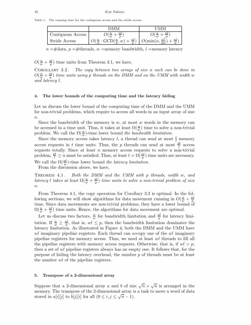
Theorem 3.1 . The contiguous access and the stride access on the DMM andthe UMM can be completed in time units shown in Table 1.

Suppose that we have two arrays a and b of size n each. The copy operation froma and b can be done by the contiguous read and the contiguous write in an obviousway. Since both the DMM and the UMM can perform the contiguous access in

10 Koji Nakano

Table 1. The running time for the contiguous access and the stride access

DMM UMM

Contiguous Access O( nw + nl

p ) O( nw + nl

p )

Stride Access O( nw ·GCD(n

p , w) + nlp ) O(min(n, n2

pw ) + nlp )

n =#data, p =#threads, w =memory bandwidth, l =memory latency

O( nw + nl

p ) time units from Theorem 3.1, we have,

Corollary 3.2 . The copy between two arrays of size n each can be done inO( n

w + nlp ) time units using p threads on the DMM and on the UMM with width w

and latency l.

4. The lower bounds of the computing time and the latency hiding

Let us discuss the lower bound of the computing time of the DMM and the UMMfor non-trivial problems, which require to access all words in an input array of sizen.

Since the bandwidth of the memory is w, at most w words in the memory canbe accessed in a time unit. Thus, it takes at least Ω( n

w ) time to solve a non-trivialproblem. We call the Ω( n

w )-time lower bound the bandwidth limitation.

Since the memory access takes latency l, a thread can send at most tl memory

access requests in t time units. Thus, the p threads can send at most ptl access

requests totally. Since at least n memory access requests to solve a non-trivialproblem, pt

l ≥ n must be satisfied. Thus, at least t = Ω(nlp ) time units are necessary.

We call the Ω(nlp )-time lower bound the latency limitation.

From the discussion above, we have,

Theorem 4.1 . Both the DMM and the UMM with p threads, width w, andlatency l takes at least Ω( n

w + nlp ) time units to solve a non-trivial problem of size

n.

From Theorem 4.1, the copy operation for Corollary 3.2 is optimal. In the fol-lowing sections, we will show algorithms for data movement running in O( n

w + nlp

time. Since data movements are non-trivial problems, they have a lower bound ofΩ( n

w + nlp ) time units. Hence, the algorithms for data movement are optimal.

Let us discuss two factors, nw for bandwidth limitation and nl

p for latency limi-

tation. If nw ≥ nl

p , that is, wl ≤ p, then the bandwidth limitation dominates thelatency limitation. As illustrated in Figure 4, both the DMM and the UMM havewl imaginary pipeline registers. Each thread can occupy one of the wl imaginarypipeline registers for memory access. Thus, we need at least wl threads to fill allthe pipeline registers with memory access requests. Otherwise, that is, if wl > p,then a set of wl pipeline registers always has an empty one. It follows that, for thepurpose of hiding the latency overhead, the number p of threads must be at leastthe number wl of the pipeline registers.

5. Transpose of a 2-dimensional array

Suppose that a 2-dimensional array a and b of size√

n × √n is arranged in thememory. The transpose of the 2-dimensional array is a task to move a word of datastored in a[i][j] to b[j][i] for all (0 ≤ i, j ≤ √n− 1).

Simple Memory Machine Models for GPUs 11

Let us start with a straightforward transpose algorithm using the contiguousaccess and the stride access. The following algorithm transposes a 2-dimensionalarray a of size

√n×√n.

[Straightforward transposing algorithm]for t← 0 to n

p − 1

for i← 0 to p− 1 do in parallelj ← (t · p + i)/

√n

k ← (t · p + i) mod√

nT (i) performs b[j][k]← a[k][j]

On the PRAM, simultaneous reading and simultaneous writing by processorscan be done in O(1) time. Hence, this straightforward transposing algorithm runsin O(n

p ) time on the PRAM. Also, it takes at least Ω(np ) time to access n words

by p processors on the PRAM. Thus, this straightforward transposing algorithm istime optimal for the PRAM.

Since the straightforward algorithm involves the stride access, it is not difficultto see that the DMM and the UMM take O( n

w ·GCD(√

n,w) + nlp ) time units and

O(min(n, n2

pw ) + nlp ) time units for transposing a 2-dimensional array, respectively.

On the DMM, GCD(√

n,w) = w if√

n is divisible by w. If this is the case, thetranspose takes O(n) time units the DMM. We will show that, regardless of thevalue of n, the transpose can be done in O( n

w + nlp ) time units both on the DMM

and on the UMM.We first show an efficient transposing algorithm on the DMM. The technique used

in this algorithm is essentially the same as the diagonal block reordering presentedin [19]. The key idea is to access the array in diagonal fashion. The details of thealgorithm are spelled out as follows:

[Transpose by the diagonal access on the DMM]for t← 0 to n

p − 1

for i← 0 to p− 1 do in parallelj ← (t · p + i)/

√n

k ← (t · p + i) mod√

nT (i) performs b[(j + k) mod

√n][k]← a[k][(j + k) mod

√n]

The readers should refer to Figure 5 for illustrating the indexes of threads readingfrom memory cells in a and writing in memory cells of b for n = p = 16 andw = 4. From the figure, we can confirm that threads T (j · 4 + 0),T (j · 4 + 1),T (j ·4 + 2),T (j · 4 + 3) read from memory cells in diagonal location of a and write tomemory cells in diagonal location of b for every j (0 ≤ j ≤ 3). Thus, reading andwriting to memory banks by w threads in a warp are different. Hence, p threadscan copy p memory cells in p

w + l− 1 time units and thus the total computing time

is ( pw + l − 1) · n

p = O( nw + nl

p ) time units. Therefore, we have,

Lemma 5.1 . The transpose of a 2-dimensional array of size√

n×√n can be donein O( n

w + nlp ) time units using p threads on the DMM with memory width w and

latency l.

Next, we will show that the transpose of a 2-dimensional array can be also donein O( n

w + nlp ) on the UMM if every thread has w local registers. As a preliminary

step, we will show that the UMM can transpose a 2-dimensional array of size w×win wl time units using w threads with each thread having a local storage of sizew. We assume that each thread has w local registers. Let ri[0], ri[1], . . . ri[w − 1]denote w local registers of T (i).

12 Koji Nakano

ba

T (0)

T (1)

T (2)

T (3)

T (4)

T (5)

T (6)

T (7)

T (8)

T (9)

T (10)

T (11)

T (12)

T (13)

T (14)

T (15)

T (0)

T (1)

T (2)

T (3)

T (4)

T (5)

T (6)

T (7)

T (8)

T (9)

T (10)

T (11)

T (12)

T (13)

T (14)

T (15)

Figure 5. Transposing on the DMM

(0,0) (0,1) (0,2) (0,3)

(1,0) (1,1) (1,2) (1,3)

(2,0) (2,1) (2,2) (2,3)

(3,0) (3,1) (3,2) (3,3)

(0,0) (0,1) (0,2) (0,3)

(1,0)(1,1) (1,2) (1,3)

(2,0) (2,1)(2,2) (2,3)

(3,0) (3,1) (3,2)(3,3)

(0,0)

(0,1)

(0,2)

(0,3)

(1,0)

(1,1)

(1,2)

(1,3)

(2,0)

(2,1)

(2,2)

(2,3)

(3,0)

(3,1)

(3,2)

(3,3)

a r0 r1 r2 r3 b

Figure 6. Transposing of a 2-dimensional array of size w × w on the UMM

[Transpose by the rotating technique on the UMM]for t← 0 to w − 1

for i← 0 to w − 1 do in parallelT (i) performs ri[t]← a[t][(t + i) mod w]

for t← 0 to w − 1for i← 0 to w − 1 do in parallel

T (i) performs b[t][(t− i) mod w]← ri[(t− i) mod w]

Let (i, j) denote the value stored in a[i][j] initially. The readers should refer toFigure 6 for illustrating how these values are transposed.

Let us confirm that the algorithm above correctly transpose the 2-dimensionalarray a. In other words, we will show that, when the algorithm terminates, b[i][j]stores (j, i). It should be clear that, the value stored in ri[t] is (t, (t + i) mod w).Since ((t − i) mod w, t) is stored in ri[(t − i) mod w], it is also stored in b[t][(t −i) mod w] when the algorithm terminates. Thus, every b[i][j] (0 ≤ i, j ≤ w − 1)stores (j, i). This completes the proof of the correctness of our transpose algorithmon the UMM.

Let us evaluate the computing time. In the reading operation ri[t] ← a[t][(t +i) mod w], w memory cells a[t][(t + 0 mod w)], a[t][(t + 1 mod w)], . . . , a[t][(t + w−1 mod w)] are in the different memory banks. Also, in the writing operation b[t][(t−i) mod w] ← ri[(t − i) mod w], w memory cells b[t][(t − 0 mod w)], b[t][(t − 1 modw)], . . . , b[t][(t − (w − 1) mod w)] are in the different memory banks. Thus, eachreading and writing operation can be done in O(l) time units and this algorithmruns in O(wl) time units.

The transpose of a larger 2-dimensional array of size√

n × √n can be done byrepeating the transpose of a 2-dimensional array of size w×w. The algorithm has

two steps. More specifically, the 2-dimensional array is partitioned into√

nw ×

√n

wsubarrays of size w × w. Let A[i][j] (0 ≤ i, j ≤ n

w − 1) denote the subarray of sizew × w. First, each subarray A[i][j] is transposed independently using w threads

Simple Memory Machine Models for GPUs 13

√n

√n

w

w

local transpose global transpose

Figure 7. Transposing on the UMM

(local transpose). After that, the corresponding words of A[i][j] and A[j][i] areswapped for all i and j in an obvious way (global transpose). Figure 7 illustratesthe transposing algorithm on the UMM.

Let us evaluate the computing time to complete the transpose of a√

n × √n2-dimensional array. Suppose that we have p (≤ n

w ) threads and partition the pthreads into p

w groups with w threads each. We assign nw2 /

pw = n

pw subarrays to

each warp of w threads. Each of the pw warps transposes each of the p

w subarraysin parallel. It takes O(w · ( p

w + l)) = O(p + wl) time units. The transposing ofpw subarrays is repeated n

pw times, the total computing time for transposing all

subarrays is npw ·O(p + wl) = O( n

w + nlp ) time units. It should have no difficulty to

confirm that the global transpose can be also done in O( nw + nl

p ) time units. Thuswe have,

Lemma 5.2 . The transpose of a 2-dimensional array of size√

n × √n can bedone in O( n

w + nlp ) time using p (w ≤ p ≤ n

w ) threads on the UMM with each threadhaving w local registers.

Finally, we will show the case that each thread of the UMM has r (< w) localregisters. We first show how we transpose a 2-dimensional array a of size

√rw×√rw

using w threads. We first partition w threads into√

rw groups of√

wr threads each.

Each group has totally√

wr · r =

√rw local registers and works as a single thread

with√

rw local registers. Each group i (0 ≤ i ≤√

wr ) with

√rw local registers can

read and store√

rw data a[0][(i+0) mod√

rw], a[1][(i+1) mod√

rw], . . . , a[√

rw−1][(i +

√rw− 1) mod

√rw] in the local registers. After that, they are written into

b[(i+0) mod√

rw][0], a[(i+1) mod√

rw][1], . . . , a[(i+√

rw−1) mod√

rw][√

rw−1].All groups read and write the arrays in turn, the transpose of a 2-dimensional arraya of size

√rw ×√rw can be done in O(l

√rw) time units.

Similarly to Lemma 5.2, we perform the transpose of a 2-dimensional array a ofsize√

n×√n. For this purpose, we partition a into√

nrw ×

√

nrw subarrays of size√

rw ×√rw. Let us evaluate the computing time. The p threads can transpose pw

subarrays in parallel in O(√

rw ·( pw + l)) = O(p

√

rw + l√

rw) time. Since we have nrw

subarrays, this transpose operation is repeated nrw/ p

w = nrp times. Thus, the local

transpose can be done in O(p√

rw+l√

rw)· nrp = O( n√rw

+nlp ·

√

wr ) = O(( n

w+nlp )·

√

wr )

time units. The global transpose is just a copy of data, it can be done in O( nw + nl

p )time units. Hence, we have,

Lemma 5.3 . The transpose of a 2-dimensional array of size√

n × √n can bedone in O(( n

w + nlp ) ·

√

wr ) time using p (w ≤ p ≤ n

r ) threads on the UMM with

each thread having r (r ≤ w) local registers.

14 Koji Nakano

Lemma 5.3 implies that the transpose by the UMM with r local registers has aoverhead of factor

√

wr .

6. Permutation of an array on the DMM

In Section 5, we have presented algorithms to transpose a 2-dimensional array onthe DMM and the UMM. The main purpose of this section is to show algorithmsthat perform any permutation of an array. Since a transpose is one of the permuta-tions, the results of this section is a generalization of those presented in Section 5.

Let a and b be one dimensional arrays of size n each, and P be a permutationof (0, 1, . . . , n − 1). The goal of permutation of an array is to copy a word of datastored in a[i] to b[P (i)] for every i (0 ≤ i ≤ n − 1). We assume that, permutationP is given in offline. We will show that, for given any permutation P , permutationof an array can be done efficiently on the DMM and the UMM.

Let us start with evaluating the performance of the straightforward permuta-tion algorithm. Suppose we need to do permutation of an array a of size n andpermutation P is given.

[Straightforward permutation algorithm]for t← 0 to n

p − 1 do

for j ← 0 to p− 1 do in paralleli← t · p + jT (j) performs b[P (i)]← a[i]

Clearly each t takes O(1) time unit on the PRAM. Hence, the straightforwardalgorithm runs in O(n

p ) time units on the PRAM.This straightforward permutation algorithm also works correctly on the DMM

and the UMM. However, it may take a lot of time to complete the permutation. Inthe worst case, this straightforward algorithm takes O(n) time units on the DMMand the UMM if all writing operation to b[P (i)] are in the same bank on the DMMor in the different address groups on the UMM. We will show that any permutationof an array of size n can be done in O( n

w + nlp ) time units on the DMM and the

UMM.If we can schedule reading/writing operations for permutation such that w

threads in a warp read from distinct banks and write in distinct banks on theDMM, the permutation can be done efficiently. For such scheduling, we use thefollowing important graph theoretic result [28, 29]:

Theorem 6.1 Konig. A regular bipartite graph with degree ρ is ρ-edge-colorable.

Figure 8 illustrates an example of a regular bipartite graph with degree 4 paintedby 4 colors. Each edge is painted by one of the 4 colors such that no node isconnected to edges with the same color. In other words, no two edges with thesame color share a node. The readers should refer to [28, 29] for the proof ofTheorem 6.1.

We show a permutation algorithm on the DMM. Suppose that a permutationP of (0, 1, . . . , n − 1) is given. We draw a bipartite graph G = (U, V,E) of P asfollows:

• U = B[0], B[1], B[2], . . . , B[w − 1] is a set of nodes each of which correspondsto a bank of a.

• V = B[0], B[1], B[2], . . . , B[w − 1] is a set of nodes each of which correspondsto a bank of b.

• For each pair source a[i] and destination b[P (i)], E has a corresponding edge

Simple Memory Machine Models for GPUs 15

Figure 8. A regular bipartite graph with degree 4

connecting B[i mod w](∈ U) and B[P (i) mod w](∈ V ).

Clearly, an edge (B[u], B[v]) (0 ≤ u, v ≤ w−1) corresponds to a word of data to becopied from bank B[u] of a to B[v] of b. Also, G = (U, V,E) is a regular bipartitegraph with degree n

w . Hence, G is nw -colorable from Theorem 6.1. Suppose that

all of the n edges in E are painted by nw colors 0, 1, . . ., n

w − 1. We determinevalue si,j (0 ≤ i ≤ n

w − 1, 0 ≤ j ≤ w − 1, 0 ≤ si,j ≤ n − 1) such that an edge(B[si,j mod w], B[P (si,j) mod w]) with color i corresponds to a pair of source a[si,j]and destination b[P (si,j)]. It should have no difficulty to confirm that, for each i,

• w banks B[si,0 mod w], B[si,1 mod w], . . . , B[si,w−1 mod w] are distinct, and

• w banks values B[P (si,0) mod w], B[P (si,1) mod w], . . . , B[P (si,w−1) mod w] aredistinct.

Thus, we have an important lemma as follows:

Lemma 6.2 . Let si,j denote a source defined above. For each i, we have, (1)a[si,0], a[si,1], . . ., a[si,w−1] are in different banks, and (2) b[P (si,0)], b[P (si,1)], . . .,b[P (si,w−1)] are in different banks.

We can perform the bank conflict-free permutation using si,j. The details arespelled out as follows.

[Permutation algorithm on the DMM]for t← 0 to n

p − 1 do

for j ← 0 to p− 1 do in paralleli← t · p + jk ← si/w,i mod w

T (j) performs b[P (k)]← a[k]

Since b[P (k)] ← a[k] are performed for all k (0 ≤ k ≤ n − 1), this algorithmperforms data movement along permutation P correctly. We will show that thispermutation algorithm terminates in O( n

w + nlp ) time units. For t = 0, warp W (q)

(0 ≤ q ≤ pw − 1) with w threads T (wq),T (wq + 1), . . . ,T (w(q + 1) − 1) performs

b[P (sq,0)] ← a[sq,0], b[P (sq,1)] ← a[sq,1], . . ., b[P (sq,w−1)] ← a[sq,w−1] in parallel.From Lemma 6.2, these w threads read from different banks in a and write todifferent banks in b. Thus, p threads complete operations for t = 0 in O( p

w + l)time units. Similarly, we can prove that the operation for every t can be done inO( p

w + l) time units. Thus the total running time is np ·O( p

w + l) = O( nw + nl

p ) timeunits. Thus, we have,

16 Koji Nakano

Theorem 6.3 . Any permutation on an array of size n can be done in O( nw + nl

p )time units using p threads on the DMM with width w and latency l.

7. Permutation of an array on the UMM

The main purpose of this section is to show a permutation algorithm on the UMM.Our permutation algorithm uses the transpose algorithm on the UMM presentedin Section 5.

We start with a small array. Suppose that we have an array a of size w andpermutation P on it. Since all elements in a are in the same address group, theycan be read/written in a time unit. Thus, any permutation of an array a of size wcan be done in O(l) time units.

Next, we show a permutation algorithm for an array a of size w2. We can considerthat a permutation is defined on a 2-dimensional array a. In other words, the goalof permutation is to move a word of data stored in a[i][j] to a[P (i ·w + j)/w][P (i ·w + j) mod w] for every i and j (0 ≤ i, j ≤ w − 1). We first show an algorithm forthe row-wise permutation which is a permutation satisfying P (i ·w + j)/w = i forall i and j. Figure 9 shows an example of row-wise permutation. In this figure, weassume that each a[i][j] is initially storing (P (i · w + j)/w,P (i · w + j) mod w]) =(i, P (i·w+j) mod w]). After the permutation, it is copied to a[i][P (i·w+j) mod w]and thus, each a[i][j] stores (i, j).

(3,0) (3,1)

(2,0)(2,1)

(0,1) (0,0)(0,3)

(1,3)

(0,2)

(1,2) (1,1)

(3,2)

(1,0)

(3,3)

(2,3) (2,2)

(3,0) (3,1)

(2,0) (2,1)

(0,1)(0,0) (0,3)

(1,3)

(0,2)

(1,2)(1,1)

(3,2)

(1,0)

(3,3)

(2,3)(2,2)

row-wisepermutation

Figure 9. Row-wise permutation

We use p threads (w ≤ p ≤ w2) partitioned into pw warps W (0),W (1), . . . ,W ( p

w−1) with w threads each. The details of the row-wise permutation algorithm are asfollows.

[Row-wise permutation algorithm]

for t← 0 to w2

p − 1

for i← 0 to pw do in parallel

W (i) performs permutation of the (t · pw + i)-th row.

Clearly, each row of an array a of size w2 corresponds to an address group. Foreach t and i, W (i) can perform a permutation of a row in O(l) time units. Hence,for each t, W (0),W (1), . . . ,W ( p

w − 1) can perform the row-wise permutation of pw

rows in O( pw + l) time units. Thus, the row-wise permutation algorithm terminates

in w2

p · (pw + l) = O(w + w2l

p ) time units. Hence we have,

Lemma 7.1 . Any row-wise permutation of a two-dimensional array of size w×wcan be done in O(w + w2l

p ) time units using p threads (w ≤ p ≤ w2) on the UMMwith width w and latency l.

We next show an algorithm for the column-wise permutation , which is a permu-tation satisfying P (i ·w + j) mod w = j for all i and j. This can be done by three

Simple Memory Machine Models for GPUs 17

steps as follows:

[Column-wise permutation on the UMM]Step 1: Transpose the two-dimensional arrayStep 2: Row-wise permute the two-dimensional arrayStep 3: Transpose the two-dimensional array

Figure 10 illustrates the data movement of the three steps. Again, in this figure, weassume that each a[i][j] is initially storing (P (i·w+j)/w,P (i·w+j) mod w) = (P (i·w+j) mod w, j). After the transpose in Step 1, a[j][i] stores (P (i ·w+j) mod w, j).The row-wise permutation is performed such that a[j][i] stores (i, j). Finally, bytransposing in Step 3, a[i][j] stores (i, j).

Since column-wise permutation can be done by transposing and row-wise per-mutation, from Lemma 5.2 and Lemma 7.1, we have,

Lemma 7.2 . Any column-wise permutation of a two-dimensional array of sizew × w can be done in O(wl) time units using w threads on the UMM with eachthread having w local registers.

(3,0)

(3,1)(2,0)

(2,1)

(0,1)

(0,0)

(0,3)

(1,3)(0,2)

(1,2)

(1,1) (3,2)(1,0) (3,3)

(2,3)

(2,2)

(3,0)

(3,1)

(2,0)

(2,1) (0,1)

(0,0)

(0,3)(1,3)

(0,2) (1,2)

(1,1)

(3,2)

(1,0)

(3,3) (2,3)

(2,2)

(3,0)

(3,1)

(2,0)

(2,1)(0,1)

(0,0)

(0,3) (1,3)

(0,2) (1,2)

(1,1)

(3,2)

(1,0)

(3,3)(2,3)

(2,2)

transpose

row-wisepermutation

(3,0) (3,1)

(2,0) (2,1)

(0,1)(0,0) (0,3)

(1,3)

(0,2)

(1,2)(1,1)

(3,2)

(1,0)

(3,3)

(2,3)(2,2)

transpose

Figure 10. Column-wise permutation

We next show any permutation of a 2-dimensional array of size w×w can be donein O(wl) time units using w threads on the UMM by the row-wise permutationand the column-wise permutation. For a given permutation P on a 2-dimensionalarray a, we draw a bipartite graph G = (U, V,E) as follows:

• U = A[0], A[1], A[2], . . . , A[w − 1] is a set of nodes each of which correspondsto an address group of source.

• V = A[0], A[1], A[2], . . . , A[w − 1] is a set of nodes each of which correspondsto an address group of destination.

• For each pair source a[i][j] and destination a[P (i ·w + j)/w][P (i ·w + j) mod w],E has a corresponding edge connecting A[i](∈ U) and A[P (i · w + j)/w](∈ V ).

For example if a word of data in a[1][3] is copied to a[2][4] by permutation P , anedge is drawn from node A[1] in U and node A[2] in V . Clearly, G is a regularbipartite graph with degree w. From Theorem 6.1, this bipartite graph can bepainted using w colors such that w edges painted by the same color never share a

18 Koji Nakano

node.Suppose that, for a given permutation P on a 2-dimensional array a of size w×w,

we have painted edges in w colors 0, 1, . . ., w − 1. Since each edge corresponds toa data stored in a, we can think that data is painted by the same color as thecorresponding edge. Permutation can be done by three steps as follows:

[Permutation on the UMM]Step 1: Row-wise permute the 2-dimensional array.Step 2: Column-wise permute the 2-dimensional array.Step 3: Row-wise permute the 2-dimensional array.

Let us see how permutation of each step is determined by edge coloring. As before,we assume that a[i][j] is storing (P (i ·w + j)/w,P (i ·w + j) mod w) and show thatafter the permutation algorithm is executed a[i][j] stores (i, j). The readers shouldrefer to Figure 11 for illustrating the data movement of the permutation algorithmfor w = 4. From the figure we can confirm the following lemma:

Lemma 7.3 . Suppose that data stored in a 2-dimensional array of w × w arepainted by w colors using edge coloring of the corresponding bipartite graph above.We have: (1) data in the same row are painted by different colors, and (2) datapainted by the same color has different row destination.

Since nodes in U are connected to w edges painted by different colors, we have(1) above. Also, since w edges painted by the same color connected to differentnodes in V , we have (2) above.

(3,0) (3,1) (2,0) (2,1)

(0,1) (0,0) (0,3) (1,3)

(0,2) (1,2) (1,1) (3,2)

(1,0) (3,3) (2,3) (2,2)

(3,0) (3,1)(2,0) (2,1)

(0,1) (0,0) (0,3)(1,3)

(0,2)(1,2) (1,1) (3,2)

(1,0)(3,3) (2,3) (2,2)

(3,0) (3,1)

(2,0) (2,1)

(0,1) (0,0) (0,3)

(1,3)

(0,2)

(1,2) (1,1)

(3,2)

(1,0)

(3,3)

(2,3) (2,2)

(3,0) (3,1)

(2,0) (2,1)

(0,1)(0,0) (0,3)

(1,3)

(0,2)

(1,2)(1,1)

(3,2)

(1,0)

(3,3)

(2,3)(2,2)

row-wisepermutation

column-wisepermutation

row-wisepermutation

Figure 11. Illustrating a data movement of the permutation algorithm on the UMM

In Step 1, row-wise permutation is performed such that data with color i (0 ≤i ≤ w− 1) are stored in the i-th column. From Lemma 7.3 (1), w data in each roware painted by w colors, Step 1 is possible. Step 2 uses column-wise permutationto move data to the final row destination. From Lemma 7.3 (2), w data in eachcolumn has different w row destination, Step 2 is possible. Finally, in Step 3, row-wise permutation is performed to move data to the final column destination.

Since the permutation algorithm on the UMM performs the row-wise permu-tation and the column-wise permutation, from Lemma 7.1 and Lemma 7.2, wehave,

Simple Memory Machine Models for GPUs 19

Lemma 7.4 . Any permutation of an array of size w2 can be done in O(wl) timeunits using w threads on the UMM with each thread having local memory of wwords.

We go on to show a permutation algorithm on a larger array a. Suppose we needto perform permutation of array a of size w4. We can consider that an array ais a 2-dimensional array of size w2 × w2. We use the permutation algorithm forLemma 7.4 to perform the row-wise permutation of the 2-dimensional array of sizew2 × w2. Similarly to the permutation algorithm for Lemma 7.4, we generate abipartite graph with G = (U, V,E) such that

• U = 0, 1, 2, . . . , w2 − 1 is a set of nodes each of which corresponds to a row ofsource.

• V = 0, 1, 2, . . . , w2 − 1 is a set of nodes each of which corresponds to a row ofdestination.

• For each pair source a[i][j] and destination a[P (i·w+j)/w2][P (i·w+j) mod w2],E has a corresponding edge connecting i(∈ U) and P (i · w + j)/w(∈ V ).

Similarly to the permutation algorithm for Lemma 7.4, any permutation of a2-dimensional array of size w2 ×w2 can be done in three steps, row-wise permuta-tion, column-wise permutation, and then row-wise permutation. The key idea is touse the permutation algorithm for Lemma 7.4 to perform the row-wise permuta-tion and the column-wise permutation. We will discuss the details of the row-wisepermutation and the column-wise permutation of a 2-dimensional array of sizew2 ×w2

We show that the row-wise permutation of a 2-dimensional array of size w2×w2

can be done in O(w3 + w4lp ) time units using p threads on the UMM. The p threads

are partitioned into pw warps. First, each of the p

w warps assigned a row of the firstpw rows performs the row-wise permutation of the first p

w row in parallel. This canbe done by the permutation algorithm for Lemma 7.4, which runs O(wl) time units.Note that, each of the w threads of a warp requests at most O(w) memory accessin the permutation algorithm for Lemma 7.4. The first memory access requests bythe p threads in p

w warps are completed pw + l time units. Since the memory access

requests by p threads are repeated O(w) times, the row-wise permutation of thefirst p

w rows is completed in O(( pw + l) ·w) = O(p+wl) time units. Since we have w2

rows, this operation is repeated w2/ pw = w3

p times. Thus, the row-wise permutation

can be done in O((p + wl) · w3

p ) = O(w3 + w4lp ) time units on the UMM.

Similarly to the row-wise permutation of a 2-dimensional array of size w × wshown in Figure 10, the column-wise permutation of a 2-dimensional array of sizew2 × w2 can be done by transpose, row-wise permutation, and transpose. Thetranspose of a 2-dimensional array of size w2 × w2 can be done in O(w3 + w4l

p )time units on the UMM from Lemma 5.2. Also, the row-wise permutation can bedone in O(w3 + w4l

p ) time units. Thus, the column-wise permutation can be done

in O(w3 + w4lp ) time units.

We are now in a position to show our permutation algorithm for a 2-dimensionalarray of size w2 × w2. Similarly to permutation of a 2-dimensional array of sizew ×w, permutation of a 2-dimensional array of size w2 ×w2 can be done in threesteps, row-wise permutation, column-wise permutation and row-wise permutation.Since each step can be done in O(w3 + w4l

p ) time on the UMM, any permutation

of a 2-dimensional array of size w2 ×w2 can be done in O(w3 + w4lp ) time units on

the UMM.We can use the same technique for a permutation of an array of size w4 × w4.

The readers should have no difficulty to confirm that any permutation can be done

20 REFERENCES

in O(w7 + w8lp ) time units on the UMM using p threads.

Repeating the same technique, we can obtain a permutation algorithm for anarray of size n = wc × wc. Permutation of a 2-dimensional array of size wc × wc

can be done by executing the row-wise permutation recursively three times and thetranspose for an array of size wc/2 × wc/2 twice. If the size n of an array satisfiesn ≤ wO(1), that is, c = O(1), then the depth of the recursion is constant. If this is

the case, the computing time is O(w2c−1 + m2clp ) = O( n

w + nlp ). Thus, we have,

Lemma 7.5 . Any permutation of an array of size n can be done in O( nw + nl

p ) time

units (w ≤ p ≤ nw ) on the UMM with each thread having w local registers provided

that n ≤ wO(1).

Finally, if each register has only r (≤ w) local registers, we can use the transposealgorithm for Lemma 5.3. If this is the case, we have,

Theorem 7.6 . Any permutation of an array of size n can be done in O(( nw +

nlp ) ·

√

wr ) time units (w ≤ p ≤ n

r ) on the UMM with each thread having r (r ≤ w)

local registers provided that n ≤ wO(1).

8. Conclusion

In this paper, we have introduced two parallel memory machines, the DiscreteMemory Machine (DMM) and the Unified Memory Machine (UMM). We firstevaluated the computing time of the contiguous access and the stride access of thememory on the DMM and the UMM. We then presented an algorithm to transposea 2-dimensional array on the DMM and the UMM. Finally, we have shown thatany permutation of an array of size n can be done in O( n

w + nlp ) time units on the

DMM and the UMM with width w and latency l. Since the computing time justinvolves the bandwidth limitation n

w and the latency limitation nlp , the permutation

algorithms are optimal.Although the DMM and the UMM are simple, they capture the characteristic

of the shared memory and the global memory of NVIDIA GPUs, Thus, these twoparallel computing models are promising for developing algorithmic techniques forNVIDIA GPUs. As a future work, we plan to implement various parallel algorithmsdeveloped for the PRAM so far on the DMM and on the UMM. Also, NVIDIAGPUs have small shared memory and large global memory. Thus, it is also inter-esting to consider a hybrid memory machine such that threads are connected to asmall memory of DMM and a large memory of UMM.

References

[1] A.V. Aho, J.D. Ullman, and J.E. Hopcroft, Data Structures and Algorithms,Addison Wesley, 1983.

[2] A. Gibbons and W. Rytter, Efficient Parallel Algorithms, Cambridge Univer-sity Press, 1988.

[3] A. Grama, G. Karypis, V. Kumar, and A. Gupta, Introduction to ParallelComputing, Addison Wesley, 2003.

[4] M.J. Quinn, Parallel Computing: Theory and Practice, McGraw-Hill, 1994.[5] W.W. Hwu, GPU Computing Gems Emerald Edition, Morgan Kaufmann,

2011.[6] D. Man, K. Uda, Y. Ito, and K. Nakano, A GPU Implementation of Computing

REFERENCES 21

Euclidean Distance Map with Efficient Memory Access, in Proc. of Interna-tional Conference on Networking and Computing, Dec., 2011, pp. 68–76.

[7] A. Uchida, Y. Ito, and K. Nakano, Fast and Accurate Template Matchingusing Pixel Rearrangement on the GPU, in Proc. of International Conferenceon Networking and Computing, Dec., 2011, pp. 153–159.

[8] Y. Ito, K. Ogawa, and K. Nakano, Fast Ellipse Detection Algorithm usingHough Transform on the GPU, in Proc. of International Conference on Net-working and Computing, Dec., 2011, pp. 313–319.

[9] K. Nishida, Y. Ito, and K. Nakano, Accelerating the Dynamic Programming forthe Matrix Chain Product on the GPU, in Proc. of International Conferenceon Networking and Computing, Dec., 2011, pp. 320–326.

[10] K. Nishida, Y. Ito, and K. Nakano, Accelerating the Dynamic Programmingfor the Optial Poygon Triangulation on the GPU, in Proc. of InternationalConference on Algorithms and Architectures for Parallel Processing (ICA3PP,LNCS 7439), Sept., 2012, pp. 1–15.

[11] NVIDIA Corporation, NVIDIA CUDA C programming guide version 4.0(2011).

[12] D. Man, K. Uda, H. Ueyama, Y. Ito, and K. Nakano, Implementations of aparallel algorithm for computing euclidean distance map in multicore proces-sors and GPUs, International Journal of Networking and Computing 1 (2011),pp. 260–276.

[13] NVIDIA Corporation, NVIDIA CUDA C best practice guide version 3.1(2010).

[14] F.T. Leighton, Introduction to Parallel Algorithms and Architectures: Arrays,Trees, Hypercubes, Morgan Kaufmann, 1991.

[15] R.H. Bisseling, Parallel Scientific Computation: A Structured Approach usingBSP and MPI, Oxford University Press, 2004.

[16] D. Culler, R. Karp, D. Patterson, A. Sahay, K.E. Schauser, E. Santos, R.Subramonian, and T. Eickenvon , LogP: towards a realistic model of paral-lel computation, in Proceedings of the fourth ACM SIGPLAN symposium onPrinciples and practice of parallel programming, 1993, pp. 1–12.

[17] R. Vaidyanathan and J.L. Trahan, Dynamic Reconfiguration: Architecturesand Algorithms, Kluwer Academic/Plenum Publishers, 2004.

[18] M.J. Flynn, Some computer organizations and their effectiveness, IEEE Trans-actions on Computers C-21 (1972), pp. 948–960.

[19] G. Ruetsch and P. Micikevicius, Optimizing matrix transpose in CUDA (2009).[20] N.K. Govindaraju, S. Larsen, J. Gray, and D. Manocha, A memory model

for scientific algorithms on graphics processors, in Proc. of the ACM/IEEEConference on Supercomputing, 2006, pp. 6–6.

[21] S. Ryoo, C.I. Rodrigues, S.S. Baghsorkhi, S.S. Stone, D.B. Kirk, and W.W. Hwumei , Optimization principles and application performance evaluationof a multithreaded GPU using CUDA, in Proc. of the 13th ACM SIGPLANSymposium on Principles and practice of parallel programming, 2008, pp. 73–82.

[22] D.T. Wang, Modern dram memory systems:performance analysis and a highperformance, power-constrained dram scheduling algorithm, Ph.D. thesis, Uni-versity of Maryland, USA, 2005.

[23] Xilinx Inc., Virtex-5 FPGA users guide (2009).[24] D.H. Lawrie, Access and alignment of data in an array processor, IEEE Trans.

on Computers C-24 (1975), pp. 1145– 1155.[25] A. Gottlieb, R. Grishman, C.P. Kruskal, K.P. McAuliffe, L. Rudolph, and M.

Snir, The nyu ultracomputer – designing an MIMD shared memory parallel

22 REFERENCES

computer, IEEE Trans. on Computers C-32 (1983), pp. 175 – 189.[26] S.G. Akl, Parallel Sorting Algorithms, Academic Press, 1985.[27] K.E. Batcher, Sorting networks and their applications, in Proc. AFIPS Spring

Joint Comput. Conf., Vol. 32, 1968, pp. 307–314.[28] K. Nakano, Optimal sorting algorithms on bus-connected processor arrays, IE-

ICE Trans. Fundamentals E76-A (1993), pp. 2008–2015.[29] R.J. Wilson, Introduction to Graph Theory, 3rd edition, Longman, 1985.