Research ArticleNumerical and Experimental Investigation on ParameterIdentification of Time-Varying Dynamical System Using HilbertTransform and Empirical Mode Decomposition

Jun Chen1 and Guanyu Zhao2

1 Department of Building Engineering State Key Laboratory for Disaster Reduction in Civil EngineeringTongji University Shanghai 200092 China

2Department of Civil Engineering KU Leuven 3000 Leuven Belgium

Correspondence should be addressed to Jun Chen cejchentongjieducn

Received 21 November 2013 Accepted 3 February 2014 Published 7 April 2014

Academic Editor Hua-Peng Chen

Copyright copy 2014 J Chen and G ZhaoThis is an open access article distributed under the Creative Commons Attribution Licensewhich permits unrestricted use distribution and reproduction in any medium provided the original work is properly cited

This paper proposes an approach to identifying time-varying structural modal parameters using the Hilbert transform andempiricalmode decompositionDefinition of instantaneous frequency and instantaneous damping ratio based onHilbert transformfor single-degree-of-freedom (SDOF) system is first introducedThe following is the definition of Hilbert damping spectrum fromwhich the time-varying damping ratio of multi-degree-of-freedom (MDOF) system can be calculated Identification proceduresfor both instantaneous frequency and damping ratios based on their definition are then introduced Applicability of the proposedidentification algorithm has been validated through several numerical examples The instantaneous frequency and damping ratiosof SDOF system under free vibration and under sinusoidal and white noise excitation have been identifiedThe proposedmethod isalso applied toMDOF system with slow and sudden changing structural parametersThe results demonstrate that when the systemmodal parameters are slowly changing the instantaneous frequency could be easily andwell identifiedwith satisfied accuracy for allcases However the instantaneous damping ratio could be extracted only when the system is lightly damped The damping resultsare better for free vibration situation than for the forced vibration cases It is also shown that the suggested method can easily trackthe abrupt change of system modal parameter under free vibration The proposed method is then applied to a 12-story short-lagshear wall structure model tested on a shaking table The instantaneous dynamic properties of the structure were identified andwere then introduced as known parameters into a finite element model Comparisons with the numerical results using constantstructural parameters demonstrate that the calculated structural responses using the identified time-varying parameters are muchcloser to the experimental results

1 Introduction

Quite some structures exhibit intrinsically time-varyingbehavior when subjected to strong excitations as earthquakeor wind or when they are damaged However most existingstructural identification techniques rest on the assumptionthat the structures are linear or time invariant They arenot readily applicable to examine the possible time-varyingbehavior during online monitoring of some civil structuresIt is therefore necessary to develop identification techniquesthat can quantify the time-varying structural behavior for thepurpose of damage detection health monitoring reliabilityand safety evaluation of structures

A mount of research has been carried out regarding theonline estimation (tracking) technique of systems with time-varying parameters Smyth et al [1] had obtained onlineestimation of the parameters of multi-degree-of-freedom(MDOF) nonlinear hysteretic systems based on the measure-ment of restoring forces Zhang et al [2] identified dynamicproperties of linear single-degree-of-freedom (SDOF) systemwith gradual changing stiffness based on empirical modedecomposition (EMD) plus Hilbert transform (HT) methodand pointed out that the steady part and transient part ofstructural dynamic responses could be separated throughHilbert spectrum analysis when the system is under sinewaveexcitation Pines and Salvino [3] proposed Hilbert damping

Hindawi Publishing CorporationMathematical Problems in EngineeringVolume 2014 Article ID 568637 15 pageshttpdxdoiorg1011552014568637

2 Mathematical Problems in Engineering

spectrum based on intrinsic mode functions decomposed bythe EMDmethodThe damping loss factor was first proposedas a joint distribution function of time and frequencyafterwards Hilbert marginal spectrum was developed andapplied to identify the damage of a 3-story shearing buildingin a shaking table test Shi and Law [4] addressed the iden-tification of linear time-varying multi-degrees-of-freedomsystems by HT+EMDThey used several numerical examplesto demonstrate the effectiveness and accuracy of the proposedmethod Basu et al [5] developed online identification oflinear time-varying stiffness of structural systems based onwavelet analysis L-P wavelet was adopted in their studyto identify MDOF system with slowly varying stiffness andsudden changing stiffness Pai et al [6] compared EMDplus Hilbert transform method with sliding window in time-frequency analysis of nonlinear signal They pointed outthat EMD plus Hilbert transform method as a self-adaptivemethod needs no basis function and has high frequencyresolution dealing with nonstationary and nonlinear signalHowever they also pointed out that Gibbs phenomenoncould lead to inaccuracy at the ends Wang and Genda [7]suggested a recursive Hilbert transformmethod for the time-varying property identification of shear-type buildings underbase excitation With known floor masses the stiffness anddamping coefficients of each floor were identified one by onefrom the top to bottom It is worth noting that the Hilberttransform plus EMD method has also been widely used inparameter identification of linear structures [8 9]The authoralso has applied the HT+EMD approach for linear identifica-tion problems as parameters identification of structures withclosed space modal properties [10] structural damage detec-tion [11] and parameter identification of an existing long-span bridge [12] We further demonstrated in Chen et al [13]that EMD is a very powerful tool in processing nonstationarysignal which is frequently encountered in time-varying iden-tification problem Though successful in numerical exam-ples experimental verifications of the abovementioned tech-niques especially for time-varying system are still rare

Inspired by the previous researches regarding the time-varying structural parameter identification problem thispaper presents an approach for identifying time-varyingstructural parameters using HT+EMD Definitions of instan-taneous frequency and damping ratios based on Hilberttransform in SDOF with time-varying parameters are firstintroduced For SDOF the time-varying parameters can beeasily obtained by its definition ForMDOF system the struc-tural responses will be first processed by EMD to obtain themodal response based on which the time-varying parameterscan be identified using the same procedure for SDOF systemExtensive numerical examples and experimental measure-ments of a large-scale 12-story building model which wastested on a shaking table have been employed to demonstratethe applicability and effectiveness of the proposed method

2 Definitions of InstantaneousParameters by Hilbert Transform

Traditionally frequency is defined as the number of occur-rences of a repeating event per unit time In the classical

Fourier transform analysis the repeating event is regarded assine or cosine wave that has constant amplitude According tothis definition any sine or cosine wave whose duration is lessthan one period cannot lead to ameaningful frequency valueHowever as we know lots of random processes in nature arenonstationary such as earthquake wave or wind speed it isdifficult for us to capture the local modulation properties ofnonstationary signals

In order to depict local properties of nonstationarysignals Leon Cohen proposed the instantaneous frequencysystematically and defined it as the first derivative of phaseangle For an arbitrary time series 119906(119905) we can always haveits Hilbert transform 120592(119905) as

120592 (119905) =

1

120587

119875119881 int

infin

minusinfin

119906 (119905)

119905 minus 120591

119889120591 (1)

where 119875119881 indicates the Cauchy principal value integralAccording to this definition 119906(119905) and 120592(119905) are actually thecomplex conjugate pair so we can have an analytic signal119909(119905) as

119909 (119905) = 119906 (119905) = 119895120592 (119905) = 119886 (119905) 119890119895120579(119905)

(2)

in which

119886 (119905) = radic119906(119905)2

+ 120592(119905)2

= |119909 (119905)| (3a)

120579 (119905) = arctan [ V (119905)119906 (119905)

] (3b)

Equation (1) defines the Hilbert transform as the convolutionintegral of 119906(119905) with 1119905 and it therefore emphasizes thelocal properties of 119906(119905) In (2) the polar coordinate expressionfurther clarifies the local nature of this representation it is thebest local fit of amplitude and phase varying trigonometricfunction to 119906(119905)

With the above Hilbert transform in (1) the instanta-neous frequency 119891

119894is defined as

119891119894=

1

2120587

119889120579

119889119905

(4)

Equation (4) can be further deduced as follows

119891119894=

1

2120587

[

1205921015840

(119905) 119906 (119905) minus 1199061015840

(119905) 120592 (119905)

1199062(119905) + 120592

2(119905)

] =

1

2120587

Im[

1199091015840

(119905)

119909 (119905)

]

=

1

2120587

[

1199091015840

(119905) 119909lowast

(119905)

|119909 (119905)|2

]

(5)

In order to clarify themeaning of (4) physically Cohen intro-duced the term ldquomonocomponent functionrdquo as a limitationon the original signal 119906(119905) which means that only when 119906(119905)is a narrow band signal could the instantaneous frequencyreflect the local vibration property

Based on the Hilbert transform and definition of instan-taneous frequency instantaneous damping ratio of SDOFsystem could also be deduced from the equation of motion

Mathematical Problems in Engineering 3

Consider the equation of motion of a SDOF system withtime-varying parameters as follows

119898(119905) (119905) + 119888 (119905) (119905) + 119896 (119905) 119906 (119905) = 0 (6)

After normalization by themass property (6) could be rewrit-ten as

(119905) + 2120585 (119905) 1205960(119905) (119905) + 120596

2

0(119905) 119906 (119905) = 0 (7)

where 1205960(119905) and 120585(119905) indicate the time-dependent frequency

and damping ratio through Hilbert transform we know thatthe analytical signal of 119906(119905) could be formed as

119911 (119905) = 119906 (119905) + 119895 (119905) = 119860 (119905) 119890119895120595(119905)

(8)

where119860(119905) and120595(119905) are regarded as the instantaneous ampli-tude and instantaneous phase angle respectivelyThefirst andsecond derivatives of analytical signal 119911(119905) could be easily gotas follows

(119905) = 119911 (119905) [

(119905)

119860 (119905)

= 119894120596 (119905)]

(119905) = 119911 (119905) [

(119905)

119860 (119905)

minus 1205962

(119905) + 2119894

(119905) 120596 (119905)

119860 (119905)

+ 119895 (119905)]

(9)

Apply HT to (7) leading to

(119905) + 2120585 (119905) 1205960(119905) (119905) + 120596

2

0(119905) 119911 (119905) = 0 (10)

Introducing (9) into (10) we get

119911 [

119860

minus 1205962

+ 1205962

0+ 2120585120596

119860

+ 119894 (2120596

119860

+ + 21205851205960120596)] = 0

(11)

Let the real part and imaginary part in (11) be equal to zerorespectively we can finally determine the time-dependentdamping ratio 120585(119905) as follows

120585 (119905) =

minus2 (119860) minus (120596)

2radic1205962minus (119860) + 2 (

11986021198602) + (119860120596)

(12)

where 119860 and 120596 are instantaneous amplitude and frequencyrespectively Therefore the instantaneous damping ratio ofSDOF systemunder zero excitation could be defined as a jointfunction of amplitude and frequency

3 Identification Methodology

With definitions of the instantaneous frequency and dampingratio for SDOF system in the previous section identifi-cation algorithms are proposed based on empirical modedecomposition method in this part The empirical modedecomposition (EMD)method was proposed by Huang et alin 1998 [14] EMD can decompose any measured signal intointrinsic mode function (IMF) that admits a well-behavedHilbert transform EMD is a self-adaptive data processing

00 05 10 15 20

Am

plitu

de

minus3minus2minus10123

Time (s)

Figure 1 Nonlinear signal 119909(119905) consists of two frequency compo-nents

method and has higher frequency resolution compared withtraditional signal processing tools in dealingwith nonstation-ary signals

Firstly in order to obtain the ldquomonocomponent functionrdquoas required byHT it is necessary to apply EMD to the originalsignal 119906(119905) to decompose it into summation of several IMFcomponents plus the final residue That is

119906 (119905) =

119873

sum

119894=1

119888119895(119905) + 119903

119873(119905) (13)

where 119888119895(119905) is intrinsicmode function which is a narrow band

signal and 119903119873(119905) is residual Therefore the multicomponent

signal 119906(119905) is represented by several monocomponent signalsIMFs Each IMF corresponds to one mode in this waydynamic responses of MDOF system could be decoupledinto several intrinsic mode responses like 119888

119895(119905) Details of the

implementation of EMDcan be found inHuang et al [14] andChen and Xu [10 12]

Having 119888119895(119905) obtained HT can be used to calculate the

instantaneous phase angle as defined in (3a)-(3b) Thenaccording to (4) three difference algorithms are introducedhere to estimate 119891

119894 and the first is forward difference

119891119894(119899) =

1

2120587

[120579 (119899 + 1) minus 120579 (119899)] (14)

The second is backward difference

119891119894(119899) =

1

2120587

[120579 (119899) minus 120579 (119899 minus 1)] (15)

The third is central difference

119891119894(119899) =

1

4120587

[120579 (119899 + 1) minus 120579 (119899 minus 1)] (16)

These three algorithms almost have the same accuracy andthey are all sensitive to noiseTherefore necessary smoothingor fitting techniques could be taken on

119891119894(119899) to eliminate

numerical errors It should be noted that the identificationresults are also sensitive to calculating parameters adopted inEMD algorithm In general a stricter decomposing standardshould be takenwhen the input signal is highly contaminated

Take a nonlinear signal 119909(119905) as example Figure 1 showsthe time history of 119909(119905)

119909 (119905) = radic2 sdot sin [2120587 sdot (4119905 + 31199052)] + radic2 sin [2120587 sdot (119905 + 21199052)] (17)

4 Mathematical Problems in Engineering

Table 1 Identification error of frequency and damping ratio at different time instant (SDOF Example 1)

Time instant (sec) Natural frequency (Hz) Damping ratio ()Theory Identify Error () Theory Identify Error ()

2 4044 4009 0 91 6186 6413 3694 3761 3742 049 4472 4435 0866 5623 5645 037 3488 3369 3428 4486 4480 013 5954 5823 21810 3572 3597 069 5249 5214 07212 5627 5606 037 3382 3408 07816 3444 3443 035 6054 5901 25820 5294 2795 470 5320 5510 348

00 05 10 15 20Time (s)

000

004

minus002000002

minus003000003

minus003000003

minus006000006

minus11

minus11

C7

C6

C5

C4

C3

C2

C1

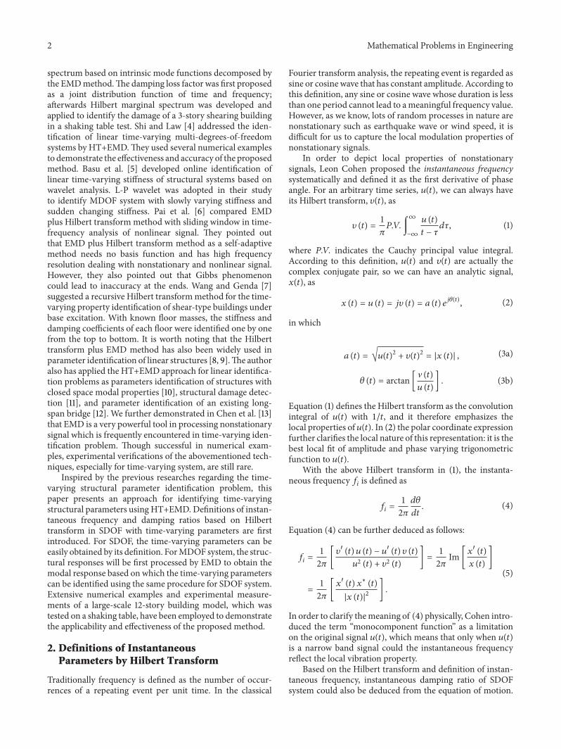
Figure 2 EMD decomposition result of signal in Figure 1

Equation (17) indicates that 119909(119905) has two modal componentsand the theoretical value of instantaneous frequency of eachcomponent is given in the following

1198911(119905) = 4 + 6119905

1198912(119905) = 1 + 4119905

(18)

After empirical mode decomposition we got seven IMFs asdepicted in Figure 2 The amplitude of the first two IMFs issignificantly larger than the last five IMFs which are actuallydue to the numerical calculation error of EMD By applyingHilbert transform to the first two IMFs we can get the instan-taneous phase angle fromwhich the instantaneous frequencycan be estimated by the forward difference algorithm given(14) Figure 3 shows the identified results compared withtheoretical ones It could be observed that identified resultsfit well with the theoretical ones

Identification of instantaneous damping ratios for SDOFsystem has been derived in (12) however it could be usedonly in free vibration cases when the system is forcedvibration EMD in conjunction with random decrementtechnique should be used first to extract the free responsesIn order to extend this method to MDOF systems Pinesand Salvino 2006 [3] proposed Hilbert damping spectrum

00 05 10 15 200

4

8

12

16

20

IdentifiedTheoretical

Time (s)

Freq

uenc

y (H

z)

Figure 3 Instantaneous frequencies 1198911(119905) and 119891

2(119905) of signal in

Figure 1

to evaluate damping he defined damping lose factor 120578(119905) =2120585(119905) and demonstrated that 120578 is a function of both frequencyand time as follows

1205782

(120596 119905) = (minus

2 (120596 119905)

119860 (120596 119905)

)

2

(1205962

+ (

(120596 119905)

119860 (120596 119905)

)

2

)

minus1

(19)

According to (19) each IMF has a time-dependent dampingloss factor 120578(119905) and as already mentioned each IMF corre-sponds to each single mode In this sense the instantaneousdamping ratios can be estimated from (19) as a marginaldistribution of time or frequency from (19) The time-dependent damping ratio for instance will be

120585 (119905) =

1

2

[119873int

119873

0

1205782

(120596 119905) 119889120596]

12

(20)

In summary the procedure of time-varying parameter iden-tification of MDOF system consists of the following threesteps First decompose the measured response of the systemby EMD into summation monocomponent signal Then foreach monocomponent signal the instantaneous frequency

Mathematical Problems in Engineering 5

0 5 10 15 20

Disp

(m

m)

Time (s)

Velo

(m

ms

)

minus10minus50510

minus15

00

15minus04

minus02

00

02

04

Acc

(mm

s2)

Figure 4 Dynamic responses of SDOF system with time-varyingparameters (Example 1)

can be estimated by (14) (15) or (16) The instantaneousdamping ratio can be estimated by (20)

4 Numerical Simulations

In order to illustrate the proposed algorithm for identificationof SDOF and MDOF systems with time-varying parametersseveral numerical examples are discussed in this sectionincluding SDOF system with slow varying and fast varyingparameters andMDOF systemwith slow varying and suddenchange parameters

41 SDOF Free Vibration SDOF system with time-varyingmass stiffness and damping is considered as follows

119898(119905) + 119888 (119905) + 119896 (119905) 119909 = 0 (21)

in which the time-varying parameters are

119898(119905) = (2 + 05119890minus01119905

) times 103 kg

119896 (119905) = (2 + cos (119905)) times 106N sdot sm

119888 (119905) = (1 + 025 sin (119905)) times 103Nm

(22)

The initial velocity and displacement of the system are10mms and 10mm respectively and time interval is set as0001 sec The free response time histories of displacementvelocity and acceleration as shown in Figure 4 were calcu-lated by fourth-order Runge-Kutta method

Take the acceleration response as the measured signal119906(119905) the instantaneous phase angle 120579(119905) and amplitude 119860(119905)can be obtained by Hilbert transform The instantaneousfrequency and damping ratios can then be identified by (14)and (12) Second-order five-point smoothing was applied tothe identified instantaneous damping ratios to reduce thenumerical noise due to difference calculation Figures 5(a)and 5(b) compare respectively the identified instantaneousfrequency and damping ratio with theoretical value

It is found that the identified instantaneous frequencyagrees very well with the theoretical value excluding theresults at endpoints The difference at endpoints is called end

0 5 10 15 202

3

4

5

6

7

8

2

3

4

5

6

7

8

Freq

uenc

y (H

z)

Time (s)

TheoreticalIdentified

(a) Instantaneous frequency

0 5 10 15 20000

001

002

003

004

005

006

007

008

Dam

ping

ratio

Time (s)

TheoreticalIdentified

(b) Instantaneous damping ratio

Figure 5 Comparison of identified time-varying parameter withtheoretical value (SDOF Example 1)

effect that is caused by Hilbert transform itself since thesignal is always cut limited while the convolution integral intheory is from minusinfin to +infin Therefore inaccuracy will occurat endpoints according to numerical difference methodsFigure 5(b) shows that the identified damping ratios arefluctuating around the theoretical value Table 1 further givesthe relative error of identified and theoretical parameters atdifferent time instants Note that the average identificationerror of frequency and damping ratio is less than 05 and3 respectively

42 SDOF Excited Vibration The equation of motion of aSDOF system under external excitation can be expressed asfollows

(119905) + 2120585 (119905) 120596 (119905) (119905) + 1205962

(119905) 119906 (119905) = minus

119886 (119905)

119898 (119905)

(23)

6 Mathematical Problems in Engineering

0 5 10 15 20

Disp

(m

m)

Time (s)

Velo

(m

s)

minus10minus50510

minus02

00

02

minus60minus30

03060

Acc

(ms2)

Figure 6 Dynamic responses of SDOF system (Example 2)

5 10 15 20

Resid

ual

Time (s)

IMF2

IMF1

minus14minus10minus6minus22

minus4minus2024

minus10minus50510

Figure 7 IMF components of acceleration response in Figure 6

where 119886(119905) is system input and 120585(119905) and 120596(119905) are time-dependent damping ratios and frequency respectively Forthe first case we assume the external input as 119886(119905) =

2119890minus004119905 sin(20120587119905+011205871199052) and the initial velocity anddisplace-

ment are zero The time-varying parameters were set as 001times that in Example 1 and the time step was 0001 sec Thedynamics responses of the system are shown in Figure 7

Figure 8 gives the Hilbert energy spectrum of the accel-eration response It can be easily observed from Figure 8 thatthere are two time scales in the response one is in the fre-quency range from 10 to 12Hz and the other is from 3 to 6HzThe second one is in accordance with the natural frequencyof the SDOF system Therefore we take the second IMF asthe free vibration response of SDOF system and followingthe above steps in the first example instantaneous frequencyand damping ratios could be easily identified The results arecompared with theoretical values as in Figures 9(a) and 9(b)

Table 2 shows relative errors at several calculation timeinstants It is found in Table 2 that identified results for fre-quency are relatively stable in the middle part of the responsewith relative error around 1 Significant errors occur atthe end due to the end effect the same as Example 1 Fordamping ratios it should be mentioned that the results arefitted by second-order 5 points smoothing method although

20

18

16

14

12

10

8

6

4

2

3 6 9 12 15 18Time (s)

Freq

uenc

y (H

z)

Figure 8 Hilbert energy spectrum for signal in Figure 7

0 5 10 15 200

2

4

6

8

10

TheoreticalIdentified

Freq

uenc

y (H

z)

Time (s)

(a) Instantaneous frequency

TheoreticalIdentified

0 5 10 15 2000000

00002

00004

00006

00008

00010

00012

00014

00016

00018

Time (s)

Dam

ping

ratio

120585

(b) Instantaneous damping ratio

Figure 9 Comparison of identified time-varying parameter withtheoretical value (SDOF Example 2)

Mathematical Problems in Engineering 7

Table 2 Identification error of frequency and damping ratio at different time instant (SDOF Example 2)

Time instant (sec) Natural frequency (Hz) Damping ratio ()Theory Identify Error () Theory Identify Error ()

2 4044 4057 031 00618 00601 2814 3761 379 074 00447 00358 1986 5623 5477 268 00348 00471 3528 4486 4547 137 00595 00562 55710 3572 3573 0024 00524 00482 80812 5627 5584 077 00338 004 18316 3444 3484 111 00605 0059 25120 5294 20 735 00532 005 599

Table 3 Identification error of frequency and damping ratio at different time instant (MDOF Example 1)

Time instant (sec) Freq (1st) Freq (2nd) Damp (1st) Damp (2nd)Theory Identify Theory Identify Theory Identify Theory Identify

2 6057 6016 14642 14592 0149 0149 0012 00124 4516 4578 12046 11988 0088 0083 0010 00116 5616 5606 17177 17171 0109 0109 0012 00148 6478 6502 15769 15934 0150 0150 0013 001310 4776 4743 11974 11974 0100 0102 0011 001112 5336 5332 17032 17054 0106 0106 0012 001116 5003 4928 12161 12109 0117 0117 0010 001020 6980 2977 17603 2000 0145 0137 0015 0016

C1

C2

K1

K2

K1

K2

Figure 10 2-DOF shear building model

the identified results are not ideal with average relative error5 the trend of time-varying damping ratios could be clearlytracked by this method White noise excitation was alsoconsidered in this example The identification accuracies forfrequency and damping were similar

43 MDOF System with Slowly Varying Parameter To illus-trate the application of the identifying methodology forMDOF systems an example of a 2DOF system has beenconsidered The system considered is a shear-building model(as shown in Figure 10) with 2 mass lumped at the two nodes1198981= 1198982= 2 + 05119890

minus005119905 kg the floor stiffness for the firstand second floor is 119896

1= (2 + sin(119905)) times 10

6Nm 1198962=

4 times (2 + cos(119905)) times 106Nm respectively The damping ratiosare assumed as time dependent with 119888

1= 01 times (1 +

05 sin 119905) times 103Nsdotsm 1198882= 005 times (1 + 05 cos 119905) times 103Nsdotsm

With initial condition 119883(0) = 10 0 10 0 (unit

0 5 10 15 20Time (s)

Velo

(m

ms

)D

isp (

mm

)

minus10

minus5

0

5

10

minus10minus05000510

minus15minus10minus5051015

Acc

(mm

s2)

Figure 11 Dynamic responses of the first floor

mm) dynamic responses of system can be calculated byfourth-order Runge-Kutta method Δ119905 = 0001 s and theresults of the first floor are shown in Figure 11 Apply EMDto the acceleration response of the first floor leading tothree IMF components as shown in Figure 12 The firstIMF corresponds to the modal response of the secondvibration mode and the second IMF corresponds to thefirst vibration mode Following the identification proceduresof SDOF system taking the two IMFs decomposed as freeresponses of SDOF system the instantaneous frequency anddamping ratios could be easily identified Figures 13(a) 13(b)

8 Mathematical Problems in Engineering

0 5 10 15 20

Resid

ual

Time (s)

IMF2

IMF1

minus10

minus5

0

5

10

minus6

minus3

0

3

6

times10minus3

20

minus2minus4minus6minus8

Figure 12 IMF components of acceleration response in Figure 11

TheoreticalIdentified

0 5 10 15 202

4

6

8

10

12

14

16

18

20

22

Freq

uenc

y (H

z)

Time (s)

(a) Instantaneous frequency

TheoreticalIdentified

0 5 10 15 200006

0008

0010

0012

0014

0016

Time (s)

Dam

ping

ratio

120585

(b) Instantaneous damping ratio of the first mode

TheoreticalIdentified

0 5 10 15 20006

008

010

012

014

016

Time (s)

Dam

ping

ratio

120585

(c) Instantaneous damping ratio of the second mode

Figure 13 Comparison of identified time-varying parameter with theoretical value (MDOF Example 1)

Mathematical Problems in Engineering 9Ve

lo (

ms

)D

isp (

mm

)

0 5 10 15

048

000005010

Time (s)

minus10minus50510

minus010

minus005

Acc

(ms2)

minus4minus8

Figure 14 Dynamic response of the first floor (MDOF Example 2)

0 5 10 150008

0010

Resid

ual

Time (s)

minus01

00

01

minus6minus3036

minus8minus4048

C3

C2

C1

Figure 15 IMF components of acceleration response in Figure 14

Table 4 Identified natural frequency damping ratio of the 12-storybuilding model

Case Naturalfrequency

Dampingratio

Frequencyreduction

Initial state 5127 00352 0Case 1 4883 00405 minus476Case 2 2930 00628 minus4285Case 3 2441 01106 minus5239

and 13(c) compare respectively the identified time-varyingfrequencies damping ration of the first and second vibrationmode with the theoretical values Table 3 further shows therelative identification error at several time instants Note thatthe frequency results fit very well with the theoretical valueswhile the damping ratio results are less ideal especially at thecurve peak or valleyThe variation trend of the instantaneousdamping can be tracked by the identification results

44MDOF Systemwith Sudden-Change Parameter To checkthe effectiveness of the method for structures with sudden-change parameter the same 2DOF system above is adopted

5 10 150

5

10

15

20

Freq

uenc

y (H

z)

Time (s)

TheoreticalIdentified

Figure 16 Comparison of identified frequency with real values(MDOF Example 2)

Figure 17 Panoramic view of the building model

Table 5 Root mean square value of measured and calculatedresponses

Wallnumber Real value Constant damping Time-dependent

dampingQ7 0779 04961 (3632) 07077 (915)Q8 06992 03781 (4592) 05391 (229)Q10 07153 04677 (3461) 06555 (836)

but assume that an abrupt change of the first floorrsquos stiffnesshappens which is

119896 =

2 times 106Nm 0 s le 119905 le 10 s

1 times 106Nm 10 s le 119905 le 15 s

(24)

10 Mathematical Problems in Engineering

Q1

Q2

Q3

Q4

Q6

Q7

Q8

Q10

Q11 Q12Q13 Q14

Q15

Q16

Q17

Q18

Q19 Q20

Q21 Q22

Q23Q24Q25Q26

3 18

3 18

3000

JJ

1550

DD

1260

A A600600 1800

(a) Wall numbering in the structural model

3 18

3 18

30003 18

3000

J

D

A

J

D

A600610 1800

3 18

600610 1800

(b) Locations of accelerometers and displacement transducer in the experiment

Figure 18 Experimental setup

with the initial conditions 119883(0) = 10 0 10 0 (unitmm) then responses of the structure are obtained by fourth-order Runge-Kutta method time interval Δ119905 = 0001 sFigure 14 shows the first floorrsquos displacement velocity andacceleration response from which three IMF componentsand one residual can be obtained by EMD (Figure 15)Figure 16 compares the identified instantaneous frequencywith the theoretical values Note that the change of frequencycan be well identified before and after the sudden change ofstiffness

5 Experimental Investigation

51 Description of the Experiment A 12-story short-lagshear wall reinforced concrete building model was testedon shanking table (see Figure 17) The structural modelwas 351m high 281m wide and 3m long as indicated inFigure 18(a) Schematic plan of standard floor of the modelwith wall numbering and measurement sensor arrangementis illustrated in Figures 18(a) and 18(b)The sensors adopted inthis test were piezoelectric accelerometers and displacement

Mathematical Problems in Engineering 11

2 4 6 8 10 12 14

Q7

Acce

lera

tion

(g)

Time (s)

minus04

minus02

00

02

04

(a)

2 4 6 8 10 12 14

Q7

Time (s)

minus4

minus2

0

2

4

Disp

lace

men

t (m

m)

(b)

Acce

lera

tion

(g)

2 4 6 8 10 12 14

00

02

minus02

Q8

Time (s)

(c)

2 4 6 8 10 12 14

Q8

Time (s)

minus4

minus2

0

2

4

Disp

lace

men

t (m

m)

(d)

2 4 6 8 10 12 14

Acce

lera

tion

(g)

00

02

minus02

Q10

Time (s)

(e)

2 4 6 8 10 12 14

Q10

Time (s)

minus4

minus2

0

2

4

Disp

lace

men

t (m

m)

(f)

Figure 19 Measured acceleration and displacement responses of wall Q7 Q8 and Q10

gauge Earthquake wave adopted in this test was El Centroearthquakewave Acceleration anddisplacement responses ofshear wall No Q7 Q8 Q10 (refer to number in Figure 18(a))on the top floor under El Centro wave are shown in Figure 19It should be noted that the displacementsmeasured in the testwere relative displacements with respect to the shake table

52 Parameter Identification White noise sweep frequencytests were carried out in the test after each loading caseUsing the acceleration records of wall Q7 the constant naturalfrequency and damping ratio can be identified by methodpreviously suggested by the author of [12] The identificationresults are given in Table 4 in which the amplitude of input

12 Mathematical Problems in Engineering

2 4 6 8 10

003004005006

2 4 6 8 1005

10152025

2 4 6 8 10

Dam

ping

Freq

(H

z)D

isp (

mm

)

(A)Time (s)

(B)Time (s)

(C)Time (s)

024

minus4minus2

(a) Wall Q7

2 4 6 8 10

003004005

Dam

ping

Time (s)(C)

2 4 6 8 1005

10152025

2 4 6 8 10

Freq

(H

z)D

isp (

mm

)

(A)Time (s)

(B)Time (s)

024

minus4minus2

(b) Wall Q8

Figure 20 The response records and identified results for Q7 and Q8 (subplot ((A) (B) and (C)) denotes the displacement time-varyingfrequency and damping ratio)

2 4 6 8 10

Acc

(mm

)

minus06minus03000306

(a)

2 4 6 8 1002468

Freq

(H

z)

(b)

2 4 6 8 10002004006008010012

Dam

ping

(c)

Figure 21 The displacement record of Q7 (a) and identified instantaneous frequency (b) and damping ratio (c)

earthquake increased from Case 1 to Case 3 (low moder-ate and high earthquake intensity) Note that the naturalfrequency has a sharp decrease from 5127Hz of the intactstructure to 2441Hz after Case 3 indicating occurrence andaccumulation of damage from test Case 1 to Case 3 It isinteresting that from Case 1 to Case 3 the damping ratioincreases from 35 to 1106 implying that the structure hasincreased energy dissipating capacity when damaged

For test Case 1 the instantaneous frequencies and damp-ing ratios are identified by the proposed method usingdisplacement responses at the top of walls Q7 and Q8 andthe identified results are given in Figure 20 It is seen thatat most part of the time duration except near the twoends of the record the identified instantaneous frequencyvaries slightly around 5Hz Test Case 2 the instantaneousfrequency and damping ratio are identified using response

of wall Q7 and the results are shown in Figure 21 It isseen that the instantaneous frequency drops quickly from6Hz to 2Hz at the beginning and then varies around 2Hzfor the rest period As for the damping ratio it goes downfrom 8 at the very beginning and varies in a range from2 to 6 and then in a range from 4 to 6 Figure 22compares the marginal damping-frequency spectrum (byintegrating (19) over time) of response of Q7 at Case 1(low level earthquake intensity) with that at Case 2 (highlevel earthquake intensity) It is observed that for low levelearthquake excitation the damping ratio changes not muchfrom 2Hz to 5Hz For high level earthquake excitationthe damping ratio is higher in lower frequency region as1Hz to 3Hz than other regions indicating that the inputenergy is mainly dissipated in vibration modes with lowerfrequency The conclusion agrees well with the experimental

Mathematical Problems in Engineering 13

2 3 4 5000

004

008

012

016

Frequency (Hz)

High levelLow level

Dam

ping

ratio

120585(

)

Figure 22 Comparison of Hilbert marginal spectrum of high andlow level earthquake excitation

observations that when the structure model was damagedmore energy will be dissipated during opening and closingof existing cracks and development of new cracks

Time-varying frequency and damping ratio of a struc-tural model under various earthquake excitations are identi-fied with the method proposed in order to testify the identi-fied results 3D finite element simulation of the shaking tabletest is performed First a 3D FE model is established withdifferent inputs of earthquake waves the displacements 119863 atdifferent shearing walls on top floor are calculated then withthe identified real time frequency and damping ratios underdifferent earthquake cases the original FEmodel is modifiedand the displacements are recalculated as 1198631015840 then 119863 and 1198631015840are compared respectively with real experimental values itis easily found that 1198631015840 is closer in amplitude to experimentalresults particularly in free vibration piece after main shock

53 FE Simulation To further compare the effect of con-stant parameters with the time-varying parameters on struc-tural response prediction a three-dimensional finite ele-ment model of the building was established as shown inFigure 23 Beam 188 element Shell63 element and Shell43element were employed to simulate beam floor and shearingwall respectively Concrete material properties were deter-mined from control specimens cast during the constructionprocedure of themodel Floor densitywas adjusted to accountfor the additional mass added to the building model in thetest Model analysis on the FEmodel was performedThe cal-culated natural frequencies of the first three vibration modesare 5075Hz 6204Hz and 6785Hz in the 119883 translationaldirection torsional direction and 119884 translational directionrespectively The relative error of the first frequency betweenFE model (5075Hz) and real model (5127Hz) is only 12which means the massstiffness ratio of the FE model is veryclose to the real one

Taking the actual record of earthquake wave in test Case1 as input to the FE model the structural responses can

XY

Z

Figure 23 3D finite element model of the test structure

be calculated for two situations first a constant dampingratio 5 is adopted and second the identified time-varyingparameters (Figure 20(a)) are used Since Rayleigh dampingmodel is used in ANSYS for the first situation the two damp-ing coefficients alpha and beta are determined as follows

120572 =

212059611205962

1205961+ 1205962

120585 =

2 times 507 times 678

507 + 678

times 2120587 times 005 = 182

120573 =

2

1205961+ 1205962

120585 =

2

(507 + 678) times 2120587

times 005 = 00013

(25)

For the second situation the identified instantaneous param-eters are introduced into the above two equations to calculatethe instantaneous damping coefficient

Figures 24 and 25 compare for the constant dampingsituation and time-varying damping respectively the cal-culated displacements of walls Q7 Q8 and Q10 with themeasured responses It is found that when constant dampingis adopted the response amplitude calculated by FE modelis much smaller than the measured value which indicatesthat the constant damping ratio of 5 is overestimated Thesignificant difference occurs in duration of 2ndash4 second wherethe calculated amplitude is only about half of the measuredones When time-varying damping is considered on theother hand the calculated responses are much closer to themeasured responses especially for the duration 6ndash10 secondswhen the structural responses could be broadly treated asfree vibration response The root-mean-square value (RMS)of the calculated responses and the measured responsesare computed and given in Table 5 The relative predictionerror for time-varying damping situation is much smallercompared to that of the constant damping situation Forresponse of wall Q7 andQ10 the relative error is nomore than10This comparison shows that time-dependent parametersby the proposed method are reasonable

14 Mathematical Problems in Engineering

2 4 6 8 10

0

2

4

ANSYSReal value

Time (s)

Disp

lace

men

t (m

m)

minus4

minus2

(a) Displacement at top of wall Q7

2 4 6 8 10

0

2

4

ANSYSReal value

Time (s)

Disp

lace

men

t (m

m)

minus2

(b) Displacement at top of wall Q8

2 4 6 8 10

ANSYSReal value

Time (s)

Disp

lace

men

t (m

m)

minus4

minus3

minus2

minus1

0

1

2

3

4

(c) Displacement at top of wall Q10

Figure 24 Displacement responses for constant damping situation

2 4 6 8 10

5

Time (s)

Disp

lace

men

t (m

m)

minus4minus3minus2minus101234

(a) Displacement at top of wall Q7

2 4 6 8 10Time (s)

Disp

lace

men

t (m

m)

minus3

minus2

minus1

0

1

2

3

4

(b) Displacement at top of wall Q8

2 4 6 8 10

Disp

lace

men

t (m

m)

Time (s)

Time-dependent dampingReal value

minus4

minus3

minus2

minus1

0

1

2

3

4

(c) Displacement at top of wall Q10

Figure 25 Displacement responses for constant damping situation

Mathematical Problems in Engineering 15

6 Conclusions

This paper suggests an approach to identifying instantaneousparameters of structures with time-dependent propertiesThe instantaneous frequency is identified by its defini-tion according to Hilbert transform For single-degree-of-freedom system the instantaneous damping ratio is iden-tified by equation derived from equation of motion withconsideration of time-varying frequency For multi-degree-of-freedom system the instantaneous damping ratio can beobtained asmarginal spectrumofHilbert damping spectrumThe empirical mode decomposition method is necessary todecompose themeasured structural response intomonocom-ponent signal thus making the calculation of instantaneousfrequency and damping spectrum reasonable The effective-ness and applicability of the proposed identification approachhave been validated by extensive numerical examples andexperimental example The results demonstrate that thesuggested method can be applied to identify instantaneousmodal features of SDOF or MDOF systems with slowlyvarying parameters

Conflict of Interests

The authors declare that there is no conflict of interestsregarding the publication of this paper

Acknowledgment

Financial support to this paper from the Project of NationalKey Technology RampD Program in the 12th Five Year Plan ofChina (2012BAJ03B02) to Jun Chen is appreciated

References

[1] A W Smyth S F Masri A G Chassiakos and T K CaugheyldquoOn-line parametric identification of MDOF nonlinear hys-teretic systemsrdquo Journal of Engineering Mechanics vol 125 no2 pp 133ndash142 1999

[2] Y Zhang J Liang and Y Hu ldquoDynamic property identificationof SDOF with gradual changing stiffness using HHTrdquo Progressin Natural Science vol 15 no 5 pp 597ndash603 2005

[3] D Pines and L Salvino ldquoStructural health monitoring usingempirical mode decomposition and the Hilbert phaserdquo Journalof Sound and Vibration vol 294 no 1-2 pp 97ndash124 2006

[4] Z Y Shi and S S Law ldquoIdentification of linear time-varyingdynamical systems using hilbert transform and empirical modedecomposition methodrdquo Journal of Applied Mechanics vol 74no 2 pp 223ndash230 2007

[5] B Basu S Nagarajaiah and A Chakraborty ldquoOnline identifi-cation of linear time-varying stiffness of structural systems bywavelet analysisrdquo Structural Health Monitoring vol 7 no 1 pp21ndash36 2008

[6] F P Pai L Huang J Hu andD R Langewisch ldquoTime-frequen-cy method for nonlinear system identification and damagedetectionrdquo Structural Health Monitoring vol 7 no 2 pp 103ndash127 2008

[7] Z Wang and C Genda ldquoRecursive Hilbert-Huang transformmethod for time-varying property identification of linear shear-type buildings under base excitationsrdquo Journal of EngineeringMechanics vol 138 no 6 pp 631ndash639 2012

[8] J N Yang Y Lei S Pan and N Huang ldquoSystem identificationof linear structures based on Hilbert-Huang spectral analysispart 1 normal modesrdquo Earthquake Engineering and StructuralDynamics vol 32 no 9 pp 1443ndash1467 2003

[9] J N Yang Y Lei S Pan and N Huang ldquoSystem identificationof linear structures based on Hilbert-Huang spectral analysispart 2 complex modesrdquo Earthquake Engineering and StructuralDynamics vol 32 no 10 pp 1533ndash1554 2003

[10] J Chen and Y L Xu ldquoIdentification of modal damping ratiosof structures with closely spaced modal frequenciesrdquo StructuralEngineering and Mechanics vol 14 no 4 pp 417ndash434 2002

[11] Y L Xu and J Chen ldquoCharacterizing nonstationary wind speedusing empirical mode decompositionrdquo Journal of StructuralEngineering vol 130 no 6 pp 912ndash920 2004

[12] J Chen Y L Xu and R C Zhang ldquoModal parameter identi-fication of Tsing Ma suspension bridge under Typhoon VictorEMD-HT methodrdquo Journal of Wind Engineering and IndustrialAerodynamics vol 92 no 10 pp 805ndash827 2004

[13] J Chen M C H Hui and Y L Xu ldquoA comparative studyof stationary and non-stationary wind models using fieldmeasurementsrdquo Boundary-LayerMeteorology vol 122 no 1 pp105ndash121 2007

[14] N E Huang Z Shen S R Long et al ldquoThe empirical modedecomposition and the Hubert spectrum for nonlinear andnon-stationary time series analysisrdquo Proceedings of the RoyalSociety A vol 454 no 1971 pp 903ndash995 1998

Submit your manuscripts athttpwwwhindawicom

Hindawi Publishing Corporationhttpwwwhindawicom Volume 2014

MathematicsJournal of

Hindawi Publishing Corporationhttpwwwhindawicom Volume 2014

Mathematical Problems in Engineering

Hindawi Publishing Corporationhttpwwwhindawicom

Differential EquationsInternational Journal of

Volume 2014

Applied MathematicsJournal of

Hindawi Publishing Corporationhttpwwwhindawicom Volume 2014

Probability and StatisticsHindawi Publishing Corporationhttpwwwhindawicom Volume 2014

Journal of

Hindawi Publishing Corporationhttpwwwhindawicom Volume 2014

Mathematical PhysicsAdvances in

Complex AnalysisJournal of

Hindawi Publishing Corporationhttpwwwhindawicom Volume 2014

OptimizationJournal of

Hindawi Publishing Corporationhttpwwwhindawicom Volume 2014

CombinatoricsHindawi Publishing Corporationhttpwwwhindawicom Volume 2014

International Journal of

Hindawi Publishing Corporationhttpwwwhindawicom Volume 2014

Operations ResearchAdvances in

Journal of

Hindawi Publishing Corporationhttpwwwhindawicom Volume 2014

Function Spaces

Abstract and Applied AnalysisHindawi Publishing Corporationhttpwwwhindawicom Volume 2014

International Journal of Mathematics and Mathematical Sciences

Hindawi Publishing Corporationhttpwwwhindawicom Volume 2014

The Scientific World JournalHindawi Publishing Corporation httpwwwhindawicom Volume 2014

Hindawi Publishing Corporationhttpwwwhindawicom Volume 2014

Algebra

Discrete Dynamics in Nature and Society

Hindawi Publishing Corporationhttpwwwhindawicom Volume 2014

Hindawi Publishing Corporationhttpwwwhindawicom Volume 2014

Decision SciencesAdvances in

Discrete MathematicsJournal of

Hindawi Publishing Corporationhttpwwwhindawicom

Volume 2014 Hindawi Publishing Corporationhttpwwwhindawicom Volume 2014

Stochastic AnalysisInternational Journal of

2 Mathematical Problems in Engineering

spectrum based on intrinsic mode functions decomposed bythe EMDmethodThe damping loss factor was first proposedas a joint distribution function of time and frequencyafterwards Hilbert marginal spectrum was developed andapplied to identify the damage of a 3-story shearing buildingin a shaking table test Shi and Law [4] addressed the iden-tification of linear time-varying multi-degrees-of-freedomsystems by HT+EMDThey used several numerical examplesto demonstrate the effectiveness and accuracy of the proposedmethod Basu et al [5] developed online identification oflinear time-varying stiffness of structural systems based onwavelet analysis L-P wavelet was adopted in their studyto identify MDOF system with slowly varying stiffness andsudden changing stiffness Pai et al [6] compared EMDplus Hilbert transform method with sliding window in time-frequency analysis of nonlinear signal They pointed outthat EMD plus Hilbert transform method as a self-adaptivemethod needs no basis function and has high frequencyresolution dealing with nonstationary and nonlinear signalHowever they also pointed out that Gibbs phenomenoncould lead to inaccuracy at the ends Wang and Genda [7]suggested a recursive Hilbert transformmethod for the time-varying property identification of shear-type buildings underbase excitation With known floor masses the stiffness anddamping coefficients of each floor were identified one by onefrom the top to bottom It is worth noting that the Hilberttransform plus EMD method has also been widely used inparameter identification of linear structures [8 9]The authoralso has applied the HT+EMD approach for linear identifica-tion problems as parameters identification of structures withclosed space modal properties [10] structural damage detec-tion [11] and parameter identification of an existing long-span bridge [12] We further demonstrated in Chen et al [13]that EMD is a very powerful tool in processing nonstationarysignal which is frequently encountered in time-varying iden-tification problem Though successful in numerical exam-ples experimental verifications of the abovementioned tech-niques especially for time-varying system are still rare

Inspired by the previous researches regarding the time-varying structural parameter identification problem thispaper presents an approach for identifying time-varyingstructural parameters using HT+EMD Definitions of instan-taneous frequency and damping ratios based on Hilberttransform in SDOF with time-varying parameters are firstintroduced For SDOF the time-varying parameters can beeasily obtained by its definition ForMDOF system the struc-tural responses will be first processed by EMD to obtain themodal response based on which the time-varying parameterscan be identified using the same procedure for SDOF systemExtensive numerical examples and experimental measure-ments of a large-scale 12-story building model which wastested on a shaking table have been employed to demonstratethe applicability and effectiveness of the proposed method

2 Definitions of InstantaneousParameters by Hilbert Transform

Traditionally frequency is defined as the number of occur-rences of a repeating event per unit time In the classical

Fourier transform analysis the repeating event is regarded assine or cosine wave that has constant amplitude According tothis definition any sine or cosine wave whose duration is lessthan one period cannot lead to ameaningful frequency valueHowever as we know lots of random processes in nature arenonstationary such as earthquake wave or wind speed it isdifficult for us to capture the local modulation properties ofnonstationary signals

In order to depict local properties of nonstationarysignals Leon Cohen proposed the instantaneous frequencysystematically and defined it as the first derivative of phaseangle For an arbitrary time series 119906(119905) we can always haveits Hilbert transform 120592(119905) as

120592 (119905) =

1

120587

119875119881 int

infin

minusinfin

119906 (119905)

119905 minus 120591

119889120591 (1)

where 119875119881 indicates the Cauchy principal value integralAccording to this definition 119906(119905) and 120592(119905) are actually thecomplex conjugate pair so we can have an analytic signal119909(119905) as

119909 (119905) = 119906 (119905) = 119895120592 (119905) = 119886 (119905) 119890119895120579(119905)

(2)

in which

119886 (119905) = radic119906(119905)2

+ 120592(119905)2

= |119909 (119905)| (3a)

120579 (119905) = arctan [ V (119905)119906 (119905)

] (3b)

Equation (1) defines the Hilbert transform as the convolutionintegral of 119906(119905) with 1119905 and it therefore emphasizes thelocal properties of 119906(119905) In (2) the polar coordinate expressionfurther clarifies the local nature of this representation it is thebest local fit of amplitude and phase varying trigonometricfunction to 119906(119905)

With the above Hilbert transform in (1) the instanta-neous frequency 119891

119894is defined as

119891119894=

1

2120587

119889120579

119889119905

(4)

Equation (4) can be further deduced as follows

119891119894=

1

2120587

[

1205921015840

(119905) 119906 (119905) minus 1199061015840

(119905) 120592 (119905)

1199062(119905) + 120592

2(119905)

] =

1

2120587

Im[

1199091015840

(119905)

119909 (119905)

]

=

1

2120587

[

1199091015840

(119905) 119909lowast

(119905)

|119909 (119905)|2

]

(5)

In order to clarify themeaning of (4) physically Cohen intro-duced the term ldquomonocomponent functionrdquo as a limitationon the original signal 119906(119905) which means that only when 119906(119905)is a narrow band signal could the instantaneous frequencyreflect the local vibration property

Based on the Hilbert transform and definition of instan-taneous frequency instantaneous damping ratio of SDOFsystem could also be deduced from the equation of motion

Mathematical Problems in Engineering 3

Consider the equation of motion of a SDOF system withtime-varying parameters as follows

119898(119905) (119905) + 119888 (119905) (119905) + 119896 (119905) 119906 (119905) = 0 (6)

After normalization by themass property (6) could be rewrit-ten as

(119905) + 2120585 (119905) 1205960(119905) (119905) + 120596

2

0(119905) 119906 (119905) = 0 (7)

where 1205960(119905) and 120585(119905) indicate the time-dependent frequency

and damping ratio through Hilbert transform we know thatthe analytical signal of 119906(119905) could be formed as

119911 (119905) = 119906 (119905) + 119895 (119905) = 119860 (119905) 119890119895120595(119905)

(8)

where119860(119905) and120595(119905) are regarded as the instantaneous ampli-tude and instantaneous phase angle respectivelyThefirst andsecond derivatives of analytical signal 119911(119905) could be easily gotas follows

(119905) = 119911 (119905) [

(119905)

119860 (119905)

= 119894120596 (119905)]

(119905) = 119911 (119905) [

(119905)

119860 (119905)

minus 1205962

(119905) + 2119894

(119905) 120596 (119905)

119860 (119905)

+ 119895 (119905)]

(9)

Apply HT to (7) leading to

(119905) + 2120585 (119905) 1205960(119905) (119905) + 120596

2

0(119905) 119911 (119905) = 0 (10)

Introducing (9) into (10) we get

119911 [

119860

minus 1205962

+ 1205962

0+ 2120585120596

119860

+ 119894 (2120596

119860

+ + 21205851205960120596)] = 0

(11)

Let the real part and imaginary part in (11) be equal to zerorespectively we can finally determine the time-dependentdamping ratio 120585(119905) as follows

120585 (119905) =

minus2 (119860) minus (120596)

2radic1205962minus (119860) + 2 (

11986021198602) + (119860120596)

(12)

where 119860 and 120596 are instantaneous amplitude and frequencyrespectively Therefore the instantaneous damping ratio ofSDOF systemunder zero excitation could be defined as a jointfunction of amplitude and frequency

3 Identification Methodology

With definitions of the instantaneous frequency and dampingratio for SDOF system in the previous section identifi-cation algorithms are proposed based on empirical modedecomposition method in this part The empirical modedecomposition (EMD)method was proposed by Huang et alin 1998 [14] EMD can decompose any measured signal intointrinsic mode function (IMF) that admits a well-behavedHilbert transform EMD is a self-adaptive data processing

00 05 10 15 20

Am

plitu

de

minus3minus2minus10123

Time (s)

Figure 1 Nonlinear signal 119909(119905) consists of two frequency compo-nents

method and has higher frequency resolution compared withtraditional signal processing tools in dealingwith nonstation-ary signals

Firstly in order to obtain the ldquomonocomponent functionrdquoas required byHT it is necessary to apply EMD to the originalsignal 119906(119905) to decompose it into summation of several IMFcomponents plus the final residue That is

119906 (119905) =

119873

sum

119894=1

119888119895(119905) + 119903

119873(119905) (13)

where 119888119895(119905) is intrinsicmode function which is a narrow band

signal and 119903119873(119905) is residual Therefore the multicomponent

signal 119906(119905) is represented by several monocomponent signalsIMFs Each IMF corresponds to one mode in this waydynamic responses of MDOF system could be decoupledinto several intrinsic mode responses like 119888

119895(119905) Details of the

implementation of EMDcan be found inHuang et al [14] andChen and Xu [10 12]

Having 119888119895(119905) obtained HT can be used to calculate the

instantaneous phase angle as defined in (3a)-(3b) Thenaccording to (4) three difference algorithms are introducedhere to estimate 119891

119894 and the first is forward difference

119891119894(119899) =

1

2120587

[120579 (119899 + 1) minus 120579 (119899)] (14)

The second is backward difference

119891119894(119899) =

1

2120587

[120579 (119899) minus 120579 (119899 minus 1)] (15)

The third is central difference

119891119894(119899) =

1

4120587

[120579 (119899 + 1) minus 120579 (119899 minus 1)] (16)

These three algorithms almost have the same accuracy andthey are all sensitive to noiseTherefore necessary smoothingor fitting techniques could be taken on

119891119894(119899) to eliminate

numerical errors It should be noted that the identificationresults are also sensitive to calculating parameters adopted inEMD algorithm In general a stricter decomposing standardshould be takenwhen the input signal is highly contaminated

Take a nonlinear signal 119909(119905) as example Figure 1 showsthe time history of 119909(119905)

119909 (119905) = radic2 sdot sin [2120587 sdot (4119905 + 31199052)] + radic2 sin [2120587 sdot (119905 + 21199052)] (17)

4 Mathematical Problems in Engineering

Table 1 Identification error of frequency and damping ratio at different time instant (SDOF Example 1)

Time instant (sec) Natural frequency (Hz) Damping ratio ()Theory Identify Error () Theory Identify Error ()

2 4044 4009 0 91 6186 6413 3694 3761 3742 049 4472 4435 0866 5623 5645 037 3488 3369 3428 4486 4480 013 5954 5823 21810 3572 3597 069 5249 5214 07212 5627 5606 037 3382 3408 07816 3444 3443 035 6054 5901 25820 5294 2795 470 5320 5510 348

00 05 10 15 20Time (s)

000

004

minus002000002

minus003000003

minus003000003

minus006000006

minus11

minus11

C7

C6

C5

C4

C3

C2

C1

Figure 2 EMD decomposition result of signal in Figure 1

Equation (17) indicates that 119909(119905) has two modal componentsand the theoretical value of instantaneous frequency of eachcomponent is given in the following

1198911(119905) = 4 + 6119905

1198912(119905) = 1 + 4119905

(18)

After empirical mode decomposition we got seven IMFs asdepicted in Figure 2 The amplitude of the first two IMFs issignificantly larger than the last five IMFs which are actuallydue to the numerical calculation error of EMD By applyingHilbert transform to the first two IMFs we can get the instan-taneous phase angle fromwhich the instantaneous frequencycan be estimated by the forward difference algorithm given(14) Figure 3 shows the identified results compared withtheoretical ones It could be observed that identified resultsfit well with the theoretical ones

Identification of instantaneous damping ratios for SDOFsystem has been derived in (12) however it could be usedonly in free vibration cases when the system is forcedvibration EMD in conjunction with random decrementtechnique should be used first to extract the free responsesIn order to extend this method to MDOF systems Pinesand Salvino 2006 [3] proposed Hilbert damping spectrum

00 05 10 15 200

4

8

12

16

20

IdentifiedTheoretical

Time (s)

Freq

uenc

y (H

z)

Figure 3 Instantaneous frequencies 1198911(119905) and 119891

2(119905) of signal in

Figure 1

to evaluate damping he defined damping lose factor 120578(119905) =2120585(119905) and demonstrated that 120578 is a function of both frequencyand time as follows

1205782

(120596 119905) = (minus

2 (120596 119905)

119860 (120596 119905)

)

2

(1205962

+ (

(120596 119905)

119860 (120596 119905)

)

2

)

minus1

(19)

According to (19) each IMF has a time-dependent dampingloss factor 120578(119905) and as already mentioned each IMF corre-sponds to each single mode In this sense the instantaneousdamping ratios can be estimated from (19) as a marginaldistribution of time or frequency from (19) The time-dependent damping ratio for instance will be

120585 (119905) =

1

2

[119873int

119873

0

1205782

(120596 119905) 119889120596]

12

(20)

In summary the procedure of time-varying parameter iden-tification of MDOF system consists of the following threesteps First decompose the measured response of the systemby EMD into summation monocomponent signal Then foreach monocomponent signal the instantaneous frequency

Mathematical Problems in Engineering 5

0 5 10 15 20

Disp

(m

m)

Time (s)

Velo

(m

ms

)

minus10minus50510

minus15

00

15minus04

minus02

00

02

04

Acc

(mm

s2)

Figure 4 Dynamic responses of SDOF system with time-varyingparameters (Example 1)

can be estimated by (14) (15) or (16) The instantaneousdamping ratio can be estimated by (20)

4 Numerical Simulations

In order to illustrate the proposed algorithm for identificationof SDOF and MDOF systems with time-varying parametersseveral numerical examples are discussed in this sectionincluding SDOF system with slow varying and fast varyingparameters andMDOF systemwith slow varying and suddenchange parameters

41 SDOF Free Vibration SDOF system with time-varyingmass stiffness and damping is considered as follows

119898(119905) + 119888 (119905) + 119896 (119905) 119909 = 0 (21)

in which the time-varying parameters are

119898(119905) = (2 + 05119890minus01119905

) times 103 kg

119896 (119905) = (2 + cos (119905)) times 106N sdot sm

119888 (119905) = (1 + 025 sin (119905)) times 103Nm

(22)

The initial velocity and displacement of the system are10mms and 10mm respectively and time interval is set as0001 sec The free response time histories of displacementvelocity and acceleration as shown in Figure 4 were calcu-lated by fourth-order Runge-Kutta method

Take the acceleration response as the measured signal119906(119905) the instantaneous phase angle 120579(119905) and amplitude 119860(119905)can be obtained by Hilbert transform The instantaneousfrequency and damping ratios can then be identified by (14)and (12) Second-order five-point smoothing was applied tothe identified instantaneous damping ratios to reduce thenumerical noise due to difference calculation Figures 5(a)and 5(b) compare respectively the identified instantaneousfrequency and damping ratio with theoretical value

It is found that the identified instantaneous frequencyagrees very well with the theoretical value excluding theresults at endpoints The difference at endpoints is called end

0 5 10 15 202

3

4

5

6

7

8

2

3

4

5

6

7

8

Freq

uenc

y (H

z)

Time (s)

TheoreticalIdentified

(a) Instantaneous frequency

0 5 10 15 20000

001

002

003

004

005

006

007

008

Dam

ping

ratio

Time (s)

TheoreticalIdentified

(b) Instantaneous damping ratio

Figure 5 Comparison of identified time-varying parameter withtheoretical value (SDOF Example 1)

effect that is caused by Hilbert transform itself since thesignal is always cut limited while the convolution integral intheory is from minusinfin to +infin Therefore inaccuracy will occurat endpoints according to numerical difference methodsFigure 5(b) shows that the identified damping ratios arefluctuating around the theoretical value Table 1 further givesthe relative error of identified and theoretical parameters atdifferent time instants Note that the average identificationerror of frequency and damping ratio is less than 05 and3 respectively

42 SDOF Excited Vibration The equation of motion of aSDOF system under external excitation can be expressed asfollows

(119905) + 2120585 (119905) 120596 (119905) (119905) + 1205962

(119905) 119906 (119905) = minus

119886 (119905)

119898 (119905)

(23)

6 Mathematical Problems in Engineering

0 5 10 15 20

Disp

(m

m)

Time (s)

Velo

(m

s)

minus10minus50510

minus02

00

02

minus60minus30

03060

Acc

(ms2)

Figure 6 Dynamic responses of SDOF system (Example 2)

5 10 15 20

Resid

ual

Time (s)

IMF2

IMF1

minus14minus10minus6minus22

minus4minus2024

minus10minus50510

Figure 7 IMF components of acceleration response in Figure 6

where 119886(119905) is system input and 120585(119905) and 120596(119905) are time-dependent damping ratios and frequency respectively Forthe first case we assume the external input as 119886(119905) =

2119890minus004119905 sin(20120587119905+011205871199052) and the initial velocity anddisplace-

ment are zero The time-varying parameters were set as 001times that in Example 1 and the time step was 0001 sec Thedynamics responses of the system are shown in Figure 7

Figure 8 gives the Hilbert energy spectrum of the accel-eration response It can be easily observed from Figure 8 thatthere are two time scales in the response one is in the fre-quency range from 10 to 12Hz and the other is from 3 to 6HzThe second one is in accordance with the natural frequencyof the SDOF system Therefore we take the second IMF asthe free vibration response of SDOF system and followingthe above steps in the first example instantaneous frequencyand damping ratios could be easily identified The results arecompared with theoretical values as in Figures 9(a) and 9(b)

Table 2 shows relative errors at several calculation timeinstants It is found in Table 2 that identified results for fre-quency are relatively stable in the middle part of the responsewith relative error around 1 Significant errors occur atthe end due to the end effect the same as Example 1 Fordamping ratios it should be mentioned that the results arefitted by second-order 5 points smoothing method although

20

18

16

14

12

10

8

6

4

2

3 6 9 12 15 18Time (s)

Freq

uenc

y (H

z)

Figure 8 Hilbert energy spectrum for signal in Figure 7

0 5 10 15 200

2

4

6

8

10

TheoreticalIdentified

Freq

uenc

y (H

z)

Time (s)

(a) Instantaneous frequency

TheoreticalIdentified

0 5 10 15 2000000

00002

00004

00006

00008

00010

00012

00014

00016

00018

Time (s)

Dam

ping

ratio

120585

(b) Instantaneous damping ratio

Figure 9 Comparison of identified time-varying parameter withtheoretical value (SDOF Example 2)

Mathematical Problems in Engineering 7

Table 2 Identification error of frequency and damping ratio at different time instant (SDOF Example 2)

Time instant (sec) Natural frequency (Hz) Damping ratio ()Theory Identify Error () Theory Identify Error ()

2 4044 4057 031 00618 00601 2814 3761 379 074 00447 00358 1986 5623 5477 268 00348 00471 3528 4486 4547 137 00595 00562 55710 3572 3573 0024 00524 00482 80812 5627 5584 077 00338 004 18316 3444 3484 111 00605 0059 25120 5294 20 735 00532 005 599

Table 3 Identification error of frequency and damping ratio at different time instant (MDOF Example 1)

Time instant (sec) Freq (1st) Freq (2nd) Damp (1st) Damp (2nd)Theory Identify Theory Identify Theory Identify Theory Identify

2 6057 6016 14642 14592 0149 0149 0012 00124 4516 4578 12046 11988 0088 0083 0010 00116 5616 5606 17177 17171 0109 0109 0012 00148 6478 6502 15769 15934 0150 0150 0013 001310 4776 4743 11974 11974 0100 0102 0011 001112 5336 5332 17032 17054 0106 0106 0012 001116 5003 4928 12161 12109 0117 0117 0010 001020 6980 2977 17603 2000 0145 0137 0015 0016

C1

C2

K1

K2

K1

K2

Figure 10 2-DOF shear building model

the identified results are not ideal with average relative error5 the trend of time-varying damping ratios could be clearlytracked by this method White noise excitation was alsoconsidered in this example The identification accuracies forfrequency and damping were similar

43 MDOF System with Slowly Varying Parameter To illus-trate the application of the identifying methodology forMDOF systems an example of a 2DOF system has beenconsidered The system considered is a shear-building model(as shown in Figure 10) with 2 mass lumped at the two nodes1198981= 1198982= 2 + 05119890

minus005119905 kg the floor stiffness for the firstand second floor is 119896

1= (2 + sin(119905)) times 10

6Nm 1198962=

4 times (2 + cos(119905)) times 106Nm respectively The damping ratiosare assumed as time dependent with 119888

1= 01 times (1 +

05 sin 119905) times 103Nsdotsm 1198882= 005 times (1 + 05 cos 119905) times 103Nsdotsm

With initial condition 119883(0) = 10 0 10 0 (unit

0 5 10 15 20Time (s)

Velo

(m

ms

)D

isp (

mm

)

minus10

minus5

0

5

10

minus10minus05000510

minus15minus10minus5051015

Acc

(mm

s2)

Figure 11 Dynamic responses of the first floor

mm) dynamic responses of system can be calculated byfourth-order Runge-Kutta method Δ119905 = 0001 s and theresults of the first floor are shown in Figure 11 Apply EMDto the acceleration response of the first floor leading tothree IMF components as shown in Figure 12 The firstIMF corresponds to the modal response of the secondvibration mode and the second IMF corresponds to thefirst vibration mode Following the identification proceduresof SDOF system taking the two IMFs decomposed as freeresponses of SDOF system the instantaneous frequency anddamping ratios could be easily identified Figures 13(a) 13(b)

8 Mathematical Problems in Engineering

0 5 10 15 20

Resid

ual

Time (s)

IMF2

IMF1

minus10

minus5

0

5

10

minus6

minus3

0

3

6

times10minus3

20

minus2minus4minus6minus8

Figure 12 IMF components of acceleration response in Figure 11

TheoreticalIdentified

0 5 10 15 202

4

6

8

10

12

14

16

18

20

22

Freq

uenc

y (H

z)

Time (s)

(a) Instantaneous frequency

TheoreticalIdentified

0 5 10 15 200006

0008

0010

0012

0014

0016

Time (s)

Dam

ping

ratio

120585

(b) Instantaneous damping ratio of the first mode

TheoreticalIdentified

0 5 10 15 20006

008

010

012

014

016

Time (s)

Dam

ping

ratio

120585

(c) Instantaneous damping ratio of the second mode

Figure 13 Comparison of identified time-varying parameter with theoretical value (MDOF Example 1)

Mathematical Problems in Engineering 9Ve

lo (

ms

)D

isp (

mm

)

0 5 10 15

048

000005010

Time (s)

minus10minus50510

minus010

minus005

Acc

(ms2)

minus4minus8

Figure 14 Dynamic response of the first floor (MDOF Example 2)

0 5 10 150008

0010

Resid

ual

Time (s)

minus01

00

01

minus6minus3036

minus8minus4048

C3

C2

C1

Figure 15 IMF components of acceleration response in Figure 14

Table 4 Identified natural frequency damping ratio of the 12-storybuilding model

Case Naturalfrequency

Dampingratio

Frequencyreduction

Initial state 5127 00352 0Case 1 4883 00405 minus476Case 2 2930 00628 minus4285Case 3 2441 01106 minus5239

and 13(c) compare respectively the identified time-varyingfrequencies damping ration of the first and second vibrationmode with the theoretical values Table 3 further shows therelative identification error at several time instants Note thatthe frequency results fit very well with the theoretical valueswhile the damping ratio results are less ideal especially at thecurve peak or valleyThe variation trend of the instantaneousdamping can be tracked by the identification results

44MDOF Systemwith Sudden-Change Parameter To checkthe effectiveness of the method for structures with sudden-change parameter the same 2DOF system above is adopted

5 10 150

5

10

15

20

Freq

uenc

y (H

z)

Time (s)

TheoreticalIdentified

Figure 16 Comparison of identified frequency with real values(MDOF Example 2)

Figure 17 Panoramic view of the building model

Table 5 Root mean square value of measured and calculatedresponses

Wallnumber Real value Constant damping Time-dependent

dampingQ7 0779 04961 (3632) 07077 (915)Q8 06992 03781 (4592) 05391 (229)Q10 07153 04677 (3461) 06555 (836)

but assume that an abrupt change of the first floorrsquos stiffnesshappens which is

119896 =

2 times 106Nm 0 s le 119905 le 10 s

1 times 106Nm 10 s le 119905 le 15 s

(24)

10 Mathematical Problems in Engineering

Q1

Q2

Q3

Q4

Q6

Q7

Q8

Q10

Q11 Q12Q13 Q14

Q15

Q16

Q17

Q18

Q19 Q20

Q21 Q22

Q23Q24Q25Q26

3 18

3 18

3000

JJ

1550

DD

1260

A A600600 1800

(a) Wall numbering in the structural model

3 18

3 18

30003 18

3000

J

D

A

J

D

A600610 1800

3 18

600610 1800

(b) Locations of accelerometers and displacement transducer in the experiment

Figure 18 Experimental setup

with the initial conditions 119883(0) = 10 0 10 0 (unitmm) then responses of the structure are obtained by fourth-order Runge-Kutta method time interval Δ119905 = 0001 sFigure 14 shows the first floorrsquos displacement velocity andacceleration response from which three IMF componentsand one residual can be obtained by EMD (Figure 15)Figure 16 compares the identified instantaneous frequencywith the theoretical values Note that the change of frequencycan be well identified before and after the sudden change ofstiffness

5 Experimental Investigation

51 Description of the Experiment A 12-story short-lagshear wall reinforced concrete building model was testedon shanking table (see Figure 17) The structural modelwas 351m high 281m wide and 3m long as indicated inFigure 18(a) Schematic plan of standard floor of the modelwith wall numbering and measurement sensor arrangementis illustrated in Figures 18(a) and 18(b)The sensors adopted inthis test were piezoelectric accelerometers and displacement

Mathematical Problems in Engineering 11

2 4 6 8 10 12 14

Q7

Acce

lera

tion

(g)

Time (s)

minus04

minus02

00

02

04

(a)

2 4 6 8 10 12 14

Q7

Time (s)

minus4

minus2

0

2

4

Disp

lace

men

t (m

m)

(b)

Acce

lera

tion

(g)

2 4 6 8 10 12 14

00

02

minus02

Q8

Time (s)

(c)

2 4 6 8 10 12 14

Q8

Time (s)

minus4

minus2

0

2

4

Disp

lace

men

t (m

m)

(d)

2 4 6 8 10 12 14

Acce

lera

tion

(g)

00

02

minus02

Q10

Time (s)

(e)

2 4 6 8 10 12 14

Q10

Time (s)

minus4

minus2

0

2

4

Disp

lace

men

t (m

m)

(f)

Figure 19 Measured acceleration and displacement responses of wall Q7 Q8 and Q10

gauge Earthquake wave adopted in this test was El Centroearthquakewave Acceleration anddisplacement responses ofshear wall No Q7 Q8 Q10 (refer to number in Figure 18(a))on the top floor under El Centro wave are shown in Figure 19It should be noted that the displacementsmeasured in the testwere relative displacements with respect to the shake table

52 Parameter Identification White noise sweep frequencytests were carried out in the test after each loading caseUsing the acceleration records of wall Q7 the constant naturalfrequency and damping ratio can be identified by methodpreviously suggested by the author of [12] The identificationresults are given in Table 4 in which the amplitude of input

12 Mathematical Problems in Engineering

2 4 6 8 10

003004005006

2 4 6 8 1005

10152025

2 4 6 8 10

Dam

ping

Freq

(H

z)D

isp (

mm

)

(A)Time (s)

(B)Time (s)

(C)Time (s)

024

minus4minus2

(a) Wall Q7

2 4 6 8 10

003004005

Dam

ping

Time (s)(C)

2 4 6 8 1005

10152025

2 4 6 8 10

Freq

(H

z)D

isp (

mm

)

(A)Time (s)

(B)Time (s)

024

minus4minus2

(b) Wall Q8

Figure 20 The response records and identified results for Q7 and Q8 (subplot ((A) (B) and (C)) denotes the displacement time-varyingfrequency and damping ratio)

2 4 6 8 10

Acc

(mm

)

minus06minus03000306

(a)

2 4 6 8 1002468

Freq

(H

z)

(b)

2 4 6 8 10002004006008010012

Dam

ping

(c)

Figure 21 The displacement record of Q7 (a) and identified instantaneous frequency (b) and damping ratio (c)

earthquake increased from Case 1 to Case 3 (low moder-ate and high earthquake intensity) Note that the naturalfrequency has a sharp decrease from 5127Hz of the intactstructure to 2441Hz after Case 3 indicating occurrence andaccumulation of damage from test Case 1 to Case 3 It isinteresting that from Case 1 to Case 3 the damping ratioincreases from 35 to 1106 implying that the structure hasincreased energy dissipating capacity when damaged

For test Case 1 the instantaneous frequencies and damp-ing ratios are identified by the proposed method usingdisplacement responses at the top of walls Q7 and Q8 andthe identified results are given in Figure 20 It is seen thatat most part of the time duration except near the twoends of the record the identified instantaneous frequencyvaries slightly around 5Hz Test Case 2 the instantaneousfrequency and damping ratio are identified using response

of wall Q7 and the results are shown in Figure 21 It isseen that the instantaneous frequency drops quickly from6Hz to 2Hz at the beginning and then varies around 2Hzfor the rest period As for the damping ratio it goes downfrom 8 at the very beginning and varies in a range from2 to 6 and then in a range from 4 to 6 Figure 22compares the marginal damping-frequency spectrum (byintegrating (19) over time) of response of Q7 at Case 1(low level earthquake intensity) with that at Case 2 (highlevel earthquake intensity) It is observed that for low levelearthquake excitation the damping ratio changes not muchfrom 2Hz to 5Hz For high level earthquake excitationthe damping ratio is higher in lower frequency region as1Hz to 3Hz than other regions indicating that the inputenergy is mainly dissipated in vibration modes with lowerfrequency The conclusion agrees well with the experimental

Mathematical Problems in Engineering 13

2 3 4 5000

004

008

012

016

Frequency (Hz)

High levelLow level

Dam

ping

ratio

120585(

)

Figure 22 Comparison of Hilbert marginal spectrum of high andlow level earthquake excitation

observations that when the structure model was damagedmore energy will be dissipated during opening and closingof existing cracks and development of new cracks

Time-varying frequency and damping ratio of a struc-tural model under various earthquake excitations are identi-fied with the method proposed in order to testify the identi-fied results 3D finite element simulation of the shaking tabletest is performed First a 3D FE model is established withdifferent inputs of earthquake waves the displacements 119863 atdifferent shearing walls on top floor are calculated then withthe identified real time frequency and damping ratios underdifferent earthquake cases the original FEmodel is modifiedand the displacements are recalculated as 1198631015840 then 119863 and 1198631015840are compared respectively with real experimental values itis easily found that 1198631015840 is closer in amplitude to experimentalresults particularly in free vibration piece after main shock

53 FE Simulation To further compare the effect of con-stant parameters with the time-varying parameters on struc-tural response prediction a three-dimensional finite ele-ment model of the building was established as shown inFigure 23 Beam 188 element Shell63 element and Shell43element were employed to simulate beam floor and shearingwall respectively Concrete material properties were deter-mined from control specimens cast during the constructionprocedure of themodel Floor densitywas adjusted to accountfor the additional mass added to the building model in thetest Model analysis on the FEmodel was performedThe cal-culated natural frequencies of the first three vibration modesare 5075Hz 6204Hz and 6785Hz in the 119883 translationaldirection torsional direction and 119884 translational directionrespectively The relative error of the first frequency betweenFE model (5075Hz) and real model (5127Hz) is only 12which means the massstiffness ratio of the FE model is veryclose to the real one

Taking the actual record of earthquake wave in test Case1 as input to the FE model the structural responses can

XY

Z

Figure 23 3D finite element model of the test structure

be calculated for two situations first a constant dampingratio 5 is adopted and second the identified time-varyingparameters (Figure 20(a)) are used Since Rayleigh dampingmodel is used in ANSYS for the first situation the two damp-ing coefficients alpha and beta are determined as follows

120572 =

212059611205962

1205961+ 1205962

120585 =

2 times 507 times 678

507 + 678

times 2120587 times 005 = 182

120573 =

2

1205961+ 1205962

120585 =

2

(507 + 678) times 2120587

times 005 = 00013

(25)

For the second situation the identified instantaneous param-eters are introduced into the above two equations to calculatethe instantaneous damping coefficient

Figures 24 and 25 compare for the constant dampingsituation and time-varying damping respectively the cal-culated displacements of walls Q7 Q8 and Q10 with themeasured responses It is found that when constant dampingis adopted the response amplitude calculated by FE modelis much smaller than the measured value which indicatesthat the constant damping ratio of 5 is overestimated Thesignificant difference occurs in duration of 2ndash4 second wherethe calculated amplitude is only about half of the measuredones When time-varying damping is considered on theother hand the calculated responses are much closer to themeasured responses especially for the duration 6ndash10 secondswhen the structural responses could be broadly treated asfree vibration response The root-mean-square value (RMS)of the calculated responses and the measured responsesare computed and given in Table 5 The relative predictionerror for time-varying damping situation is much smallercompared to that of the constant damping situation Forresponse of wall Q7 andQ10 the relative error is nomore than10This comparison shows that time-dependent parametersby the proposed method are reasonable

14 Mathematical Problems in Engineering

2 4 6 8 10

0

2

4

ANSYSReal value

Time (s)

Disp

lace

men

t (m

m)

minus4

minus2

(a) Displacement at top of wall Q7

2 4 6 8 10

0

2

4

ANSYSReal value

Time (s)

Disp

lace

men

t (m

m)

minus2

(b) Displacement at top of wall Q8

2 4 6 8 10

ANSYSReal value

Time (s)

Disp

lace

men

t (m

m)

minus4

minus3

minus2

minus1

0

1

2

3

4

(c) Displacement at top of wall Q10

Figure 24 Displacement responses for constant damping situation

2 4 6 8 10

5

Time (s)

Disp

lace

men

t (m

m)

minus4minus3minus2minus101234

(a) Displacement at top of wall Q7

2 4 6 8 10Time (s)

Disp

lace

men

t (m

m)

minus3

minus2

minus1

0

1

2

3

4

(b) Displacement at top of wall Q8

2 4 6 8 10

Disp

lace

men

t (m

m)

Time (s)

Time-dependent dampingReal value

minus4

minus3

minus2

minus1

0

1

2

3

4

(c) Displacement at top of wall Q10

Figure 25 Displacement responses for constant damping situation

Mathematical Problems in Engineering 15

6 Conclusions

This paper suggests an approach to identifying instantaneousparameters of structures with time-dependent propertiesThe instantaneous frequency is identified by its defini-tion according to Hilbert transform For single-degree-of-freedom system the instantaneous damping ratio is iden-tified by equation derived from equation of motion withconsideration of time-varying frequency For multi-degree-of-freedom system the instantaneous damping ratio can beobtained asmarginal spectrumofHilbert damping spectrumThe empirical mode decomposition method is necessary todecompose themeasured structural response intomonocom-ponent signal thus making the calculation of instantaneousfrequency and damping spectrum reasonable The effective-ness and applicability of the proposed identification approachhave been validated by extensive numerical examples andexperimental example The results demonstrate that thesuggested method can be applied to identify instantaneousmodal features of SDOF or MDOF systems with slowlyvarying parameters

Conflict of Interests

The authors declare that there is no conflict of interestsregarding the publication of this paper

Acknowledgment

Financial support to this paper from the Project of NationalKey Technology RampD Program in the 12th Five Year Plan ofChina (2012BAJ03B02) to Jun Chen is appreciated

References

[1] A W Smyth S F Masri A G Chassiakos and T K CaugheyldquoOn-line parametric identification of MDOF nonlinear hys-teretic systemsrdquo Journal of Engineering Mechanics vol 125 no2 pp 133ndash142 1999

[2] Y Zhang J Liang and Y Hu ldquoDynamic property identificationof SDOF with gradual changing stiffness using HHTrdquo Progressin Natural Science vol 15 no 5 pp 597ndash603 2005

[3] D Pines and L Salvino ldquoStructural health monitoring usingempirical mode decomposition and the Hilbert phaserdquo Journalof Sound and Vibration vol 294 no 1-2 pp 97ndash124 2006

[4] Z Y Shi and S S Law ldquoIdentification of linear time-varyingdynamical systems using hilbert transform and empirical modedecomposition methodrdquo Journal of Applied Mechanics vol 74no 2 pp 223ndash230 2007

[5] B Basu S Nagarajaiah and A Chakraborty ldquoOnline identifi-cation of linear time-varying stiffness of structural systems bywavelet analysisrdquo Structural Health Monitoring vol 7 no 1 pp21ndash36 2008

[6] F P Pai L Huang J Hu andD R Langewisch ldquoTime-frequen-cy method for nonlinear system identification and damagedetectionrdquo Structural Health Monitoring vol 7 no 2 pp 103ndash127 2008

[7] Z Wang and C Genda ldquoRecursive Hilbert-Huang transformmethod for time-varying property identification of linear shear-type buildings under base excitationsrdquo Journal of EngineeringMechanics vol 138 no 6 pp 631ndash639 2012

[8] J N Yang Y Lei S Pan and N Huang ldquoSystem identificationof linear structures based on Hilbert-Huang spectral analysispart 1 normal modesrdquo Earthquake Engineering and StructuralDynamics vol 32 no 9 pp 1443ndash1467 2003

[9] J N Yang Y Lei S Pan and N Huang ldquoSystem identificationof linear structures based on Hilbert-Huang spectral analysispart 2 complex modesrdquo Earthquake Engineering and StructuralDynamics vol 32 no 10 pp 1533ndash1554 2003

[10] J Chen and Y L Xu ldquoIdentification of modal damping ratiosof structures with closely spaced modal frequenciesrdquo StructuralEngineering and Mechanics vol 14 no 4 pp 417ndash434 2002

[11] Y L Xu and J Chen ldquoCharacterizing nonstationary wind speedusing empirical mode decompositionrdquo Journal of StructuralEngineering vol 130 no 6 pp 912ndash920 2004

[12] J Chen Y L Xu and R C Zhang ldquoModal parameter identi-fication of Tsing Ma suspension bridge under Typhoon VictorEMD-HT methodrdquo Journal of Wind Engineering and IndustrialAerodynamics vol 92 no 10 pp 805ndash827 2004

[13] J Chen M C H Hui and Y L Xu ldquoA comparative studyof stationary and non-stationary wind models using fieldmeasurementsrdquo Boundary-LayerMeteorology vol 122 no 1 pp105ndash121 2007

[14] N E Huang Z Shen S R Long et al ldquoThe empirical modedecomposition and the Hubert spectrum for nonlinear andnon-stationary time series analysisrdquo Proceedings of the RoyalSociety A vol 454 no 1971 pp 903ndash995 1998

Submit your manuscripts athttpwwwhindawicom

Hindawi Publishing Corporationhttpwwwhindawicom Volume 2014

MathematicsJournal of

Hindawi Publishing Corporationhttpwwwhindawicom Volume 2014

Mathematical Problems in Engineering

Hindawi Publishing Corporationhttpwwwhindawicom

Differential EquationsInternational Journal of

Volume 2014

Applied MathematicsJournal of

Hindawi Publishing Corporationhttpwwwhindawicom Volume 2014

Probability and StatisticsHindawi Publishing Corporationhttpwwwhindawicom Volume 2014

Journal of

Hindawi Publishing Corporationhttpwwwhindawicom Volume 2014

Mathematical PhysicsAdvances in

Complex AnalysisJournal of

Hindawi Publishing Corporationhttpwwwhindawicom Volume 2014

OptimizationJournal of

Hindawi Publishing Corporationhttpwwwhindawicom Volume 2014

CombinatoricsHindawi Publishing Corporationhttpwwwhindawicom Volume 2014

International Journal of

Hindawi Publishing Corporationhttpwwwhindawicom Volume 2014

Operations ResearchAdvances in

Journal of

Hindawi Publishing Corporationhttpwwwhindawicom Volume 2014

Function Spaces

Abstract and Applied AnalysisHindawi Publishing Corporationhttpwwwhindawicom Volume 2014

International Journal of Mathematics and Mathematical Sciences

Hindawi Publishing Corporationhttpwwwhindawicom Volume 2014

The Scientific World JournalHindawi Publishing Corporation httpwwwhindawicom Volume 2014

Hindawi Publishing Corporationhttpwwwhindawicom Volume 2014

Algebra

Discrete Dynamics in Nature and Society

Hindawi Publishing Corporationhttpwwwhindawicom Volume 2014

Hindawi Publishing Corporationhttpwwwhindawicom Volume 2014

Decision SciencesAdvances in

Discrete MathematicsJournal of

Hindawi Publishing Corporationhttpwwwhindawicom

Volume 2014 Hindawi Publishing Corporationhttpwwwhindawicom Volume 2014

Stochastic AnalysisInternational Journal of

Mathematical Problems in Engineering 3

Consider the equation of motion of a SDOF system withtime-varying parameters as follows

119898(119905) (119905) + 119888 (119905) (119905) + 119896 (119905) 119906 (119905) = 0 (6)

After normalization by themass property (6) could be rewrit-ten as

(119905) + 2120585 (119905) 1205960(119905) (119905) + 120596

2

0(119905) 119906 (119905) = 0 (7)

where 1205960(119905) and 120585(119905) indicate the time-dependent frequency

and damping ratio through Hilbert transform we know thatthe analytical signal of 119906(119905) could be formed as

119911 (119905) = 119906 (119905) + 119895 (119905) = 119860 (119905) 119890119895120595(119905)

(8)

where119860(119905) and120595(119905) are regarded as the instantaneous ampli-tude and instantaneous phase angle respectivelyThefirst andsecond derivatives of analytical signal 119911(119905) could be easily gotas follows

(119905) = 119911 (119905) [

(119905)

119860 (119905)

= 119894120596 (119905)]

(119905) = 119911 (119905) [

(119905)

119860 (119905)

minus 1205962

(119905) + 2119894

(119905) 120596 (119905)

119860 (119905)

+ 119895 (119905)]

(9)

Apply HT to (7) leading to

(119905) + 2120585 (119905) 1205960(119905) (119905) + 120596

2

0(119905) 119911 (119905) = 0 (10)

Introducing (9) into (10) we get

119911 [

119860

minus 1205962

+ 1205962

0+ 2120585120596

119860

+ 119894 (2120596

119860

+ + 21205851205960120596)] = 0

(11)

Let the real part and imaginary part in (11) be equal to zerorespectively we can finally determine the time-dependentdamping ratio 120585(119905) as follows

120585 (119905) =

minus2 (119860) minus (120596)

2radic1205962minus (119860) + 2 (

11986021198602) + (119860120596)

(12)

where 119860 and 120596 are instantaneous amplitude and frequencyrespectively Therefore the instantaneous damping ratio ofSDOF systemunder zero excitation could be defined as a jointfunction of amplitude and frequency

3 Identification Methodology

With definitions of the instantaneous frequency and dampingratio for SDOF system in the previous section identifi-cation algorithms are proposed based on empirical modedecomposition method in this part The empirical modedecomposition (EMD)method was proposed by Huang et alin 1998 [14] EMD can decompose any measured signal intointrinsic mode function (IMF) that admits a well-behavedHilbert transform EMD is a self-adaptive data processing

00 05 10 15 20

Am

plitu

de

minus3minus2minus10123

Time (s)

Figure 1 Nonlinear signal 119909(119905) consists of two frequency compo-nents

method and has higher frequency resolution compared withtraditional signal processing tools in dealingwith nonstation-ary signals

Firstly in order to obtain the ldquomonocomponent functionrdquoas required byHT it is necessary to apply EMD to the originalsignal 119906(119905) to decompose it into summation of several IMFcomponents plus the final residue That is

119906 (119905) =

119873

sum

119894=1

119888119895(119905) + 119903

119873(119905) (13)

where 119888119895(119905) is intrinsicmode function which is a narrow band

signal and 119903119873(119905) is residual Therefore the multicomponent

signal 119906(119905) is represented by several monocomponent signalsIMFs Each IMF corresponds to one mode in this waydynamic responses of MDOF system could be decoupledinto several intrinsic mode responses like 119888

119895(119905) Details of the

implementation of EMDcan be found inHuang et al [14] andChen and Xu [10 12]

Having 119888119895(119905) obtained HT can be used to calculate the

instantaneous phase angle as defined in (3a)-(3b) Thenaccording to (4) three difference algorithms are introducedhere to estimate 119891

119894 and the first is forward difference

119891119894(119899) =

1

2120587

[120579 (119899 + 1) minus 120579 (119899)] (14)

The second is backward difference

119891119894(119899) =

1

2120587

[120579 (119899) minus 120579 (119899 minus 1)] (15)

The third is central difference

119891119894(119899) =

1

4120587

[120579 (119899 + 1) minus 120579 (119899 minus 1)] (16)

These three algorithms almost have the same accuracy andthey are all sensitive to noiseTherefore necessary smoothingor fitting techniques could be taken on

119891119894(119899) to eliminate

numerical errors It should be noted that the identificationresults are also sensitive to calculating parameters adopted inEMD algorithm In general a stricter decomposing standardshould be takenwhen the input signal is highly contaminated

Take a nonlinear signal 119909(119905) as example Figure 1 showsthe time history of 119909(119905)

119909 (119905) = radic2 sdot sin [2120587 sdot (4119905 + 31199052)] + radic2 sin [2120587 sdot (119905 + 21199052)] (17)

4 Mathematical Problems in Engineering

Table 1 Identification error of frequency and damping ratio at different time instant (SDOF Example 1)

Time instant (sec) Natural frequency (Hz) Damping ratio ()Theory Identify Error () Theory Identify Error ()

2 4044 4009 0 91 6186 6413 3694 3761 3742 049 4472 4435 0866 5623 5645 037 3488 3369 3428 4486 4480 013 5954 5823 21810 3572 3597 069 5249 5214 07212 5627 5606 037 3382 3408 07816 3444 3443 035 6054 5901 25820 5294 2795 470 5320 5510 348

00 05 10 15 20Time (s)

000

004

minus002000002

minus003000003

minus003000003

minus006000006

minus11

minus11

C7

C6

C5

C4

C3

C2

C1

Figure 2 EMD decomposition result of signal in Figure 1

Equation (17) indicates that 119909(119905) has two modal componentsand the theoretical value of instantaneous frequency of eachcomponent is given in the following

1198911(119905) = 4 + 6119905

1198912(119905) = 1 + 4119905

(18)

After empirical mode decomposition we got seven IMFs asdepicted in Figure 2 The amplitude of the first two IMFs issignificantly larger than the last five IMFs which are actuallydue to the numerical calculation error of EMD By applyingHilbert transform to the first two IMFs we can get the instan-taneous phase angle fromwhich the instantaneous frequencycan be estimated by the forward difference algorithm given(14) Figure 3 shows the identified results compared withtheoretical ones It could be observed that identified resultsfit well with the theoretical ones

Identification of instantaneous damping ratios for SDOFsystem has been derived in (12) however it could be usedonly in free vibration cases when the system is forcedvibration EMD in conjunction with random decrementtechnique should be used first to extract the free responsesIn order to extend this method to MDOF systems Pinesand Salvino 2006 [3] proposed Hilbert damping spectrum

00 05 10 15 200

4

8

12

16

20

IdentifiedTheoretical

Time (s)

Freq

uenc

y (H

z)

Figure 3 Instantaneous frequencies 1198911(119905) and 119891

2(119905) of signal in

Figure 1

to evaluate damping he defined damping lose factor 120578(119905) =2120585(119905) and demonstrated that 120578 is a function of both frequencyand time as follows

1205782

(120596 119905) = (minus

2 (120596 119905)

119860 (120596 119905)

)

2

(1205962

+ (

(120596 119905)

119860 (120596 119905)

)

2

)

minus1

(19)

According to (19) each IMF has a time-dependent dampingloss factor 120578(119905) and as already mentioned each IMF corre-sponds to each single mode In this sense the instantaneousdamping ratios can be estimated from (19) as a marginaldistribution of time or frequency from (19) The time-dependent damping ratio for instance will be

120585 (119905) =

1

2

[119873int

119873

0

1205782

(120596 119905) 119889120596]

12

(20)

In summary the procedure of time-varying parameter iden-tification of MDOF system consists of the following threesteps First decompose the measured response of the systemby EMD into summation monocomponent signal Then foreach monocomponent signal the instantaneous frequency

Mathematical Problems in Engineering 5

0 5 10 15 20

Disp

(m

m)

Time (s)

Velo

(m

ms

)

minus10minus50510

minus15

00

15minus04

minus02

00

02

04

Acc

(mm

s2)

Figure 4 Dynamic responses of SDOF system with time-varyingparameters (Example 1)

can be estimated by (14) (15) or (16) The instantaneousdamping ratio can be estimated by (20)

4 Numerical Simulations

In order to illustrate the proposed algorithm for identificationof SDOF and MDOF systems with time-varying parametersseveral numerical examples are discussed in this sectionincluding SDOF system with slow varying and fast varyingparameters andMDOF systemwith slow varying and suddenchange parameters

41 SDOF Free Vibration SDOF system with time-varyingmass stiffness and damping is considered as follows

119898(119905) + 119888 (119905) + 119896 (119905) 119909 = 0 (21)

in which the time-varying parameters are

119898(119905) = (2 + 05119890minus01119905

) times 103 kg

119896 (119905) = (2 + cos (119905)) times 106N sdot sm

119888 (119905) = (1 + 025 sin (119905)) times 103Nm

(22)

The initial velocity and displacement of the system are10mms and 10mm respectively and time interval is set as0001 sec The free response time histories of displacementvelocity and acceleration as shown in Figure 4 were calcu-lated by fourth-order Runge-Kutta method

Take the acceleration response as the measured signal119906(119905) the instantaneous phase angle 120579(119905) and amplitude 119860(119905)can be obtained by Hilbert transform The instantaneousfrequency and damping ratios can then be identified by (14)and (12) Second-order five-point smoothing was applied tothe identified instantaneous damping ratios to reduce thenumerical noise due to difference calculation Figures 5(a)and 5(b) compare respectively the identified instantaneousfrequency and damping ratio with theoretical value

It is found that the identified instantaneous frequencyagrees very well with the theoretical value excluding theresults at endpoints The difference at endpoints is called end

0 5 10 15 202

3

4

5

6

7

8

2

3

4

5

6

7

8

Freq

uenc

y (H

z)

Time (s)

TheoreticalIdentified

(a) Instantaneous frequency

0 5 10 15 20000

001

002

003

004

005

006

007

008

Dam

ping

ratio

Time (s)

TheoreticalIdentified

(b) Instantaneous damping ratio

Figure 5 Comparison of identified time-varying parameter withtheoretical value (SDOF Example 1)

effect that is caused by Hilbert transform itself since thesignal is always cut limited while the convolution integral intheory is from minusinfin to +infin Therefore inaccuracy will occurat endpoints according to numerical difference methodsFigure 5(b) shows that the identified damping ratios arefluctuating around the theoretical value Table 1 further givesthe relative error of identified and theoretical parameters atdifferent time instants Note that the average identificationerror of frequency and damping ratio is less than 05 and3 respectively

42 SDOF Excited Vibration The equation of motion of aSDOF system under external excitation can be expressed asfollows

(119905) + 2120585 (119905) 120596 (119905) (119905) + 1205962

(119905) 119906 (119905) = minus

119886 (119905)

119898 (119905)

(23)

6 Mathematical Problems in Engineering

0 5 10 15 20

Disp

(m

m)

Time (s)

Velo

(m

s)

minus10minus50510

minus02

00

02

minus60minus30

03060

Acc

(ms2)

Figure 6 Dynamic responses of SDOF system (Example 2)

5 10 15 20

Resid

ual

Time (s)

IMF2

IMF1

minus14minus10minus6minus22

minus4minus2024

minus10minus50510

Figure 7 IMF components of acceleration response in Figure 6

where 119886(119905) is system input and 120585(119905) and 120596(119905) are time-dependent damping ratios and frequency respectively Forthe first case we assume the external input as 119886(119905) =

2119890minus004119905 sin(20120587119905+011205871199052) and the initial velocity anddisplace-

ment are zero The time-varying parameters were set as 001times that in Example 1 and the time step was 0001 sec Thedynamics responses of the system are shown in Figure 7

Figure 8 gives the Hilbert energy spectrum of the accel-eration response It can be easily observed from Figure 8 thatthere are two time scales in the response one is in the fre-quency range from 10 to 12Hz and the other is from 3 to 6HzThe second one is in accordance with the natural frequencyof the SDOF system Therefore we take the second IMF asthe free vibration response of SDOF system and followingthe above steps in the first example instantaneous frequencyand damping ratios could be easily identified The results arecompared with theoretical values as in Figures 9(a) and 9(b)

Table 2 shows relative errors at several calculation timeinstants It is found in Table 2 that identified results for fre-quency are relatively stable in the middle part of the responsewith relative error around 1 Significant errors occur atthe end due to the end effect the same as Example 1 Fordamping ratios it should be mentioned that the results arefitted by second-order 5 points smoothing method although

20

18

16

14

12

10

8

6

4

2

3 6 9 12 15 18Time (s)

Freq

uenc

y (H

z)

Figure 8 Hilbert energy spectrum for signal in Figure 7

0 5 10 15 200

2

4

6

8

10

TheoreticalIdentified

Freq

uenc

y (H

z)

Time (s)

(a) Instantaneous frequency

TheoreticalIdentified

0 5 10 15 2000000

00002

00004

00006

00008

00010

00012

00014

00016

00018

Time (s)

Dam

ping

ratio

120585

(b) Instantaneous damping ratio

Figure 9 Comparison of identified time-varying parameter withtheoretical value (SDOF Example 2)

Mathematical Problems in Engineering 7

Table 2 Identification error of frequency and damping ratio at different time instant (SDOF Example 2)

Time instant (sec) Natural frequency (Hz) Damping ratio ()Theory Identify Error () Theory Identify Error ()

2 4044 4057 031 00618 00601 2814 3761 379 074 00447 00358 1986 5623 5477 268 00348 00471 3528 4486 4547 137 00595 00562 55710 3572 3573 0024 00524 00482 80812 5627 5584 077 00338 004 18316 3444 3484 111 00605 0059 25120 5294 20 735 00532 005 599

Table 3 Identification error of frequency and damping ratio at different time instant (MDOF Example 1)

Time instant (sec) Freq (1st) Freq (2nd) Damp (1st) Damp (2nd)Theory Identify Theory Identify Theory Identify Theory Identify

2 6057 6016 14642 14592 0149 0149 0012 00124 4516 4578 12046 11988 0088 0083 0010 00116 5616 5606 17177 17171 0109 0109 0012 00148 6478 6502 15769 15934 0150 0150 0013 001310 4776 4743 11974 11974 0100 0102 0011 001112 5336 5332 17032 17054 0106 0106 0012 001116 5003 4928 12161 12109 0117 0117 0010 001020 6980 2977 17603 2000 0145 0137 0015 0016

C1

C2

K1

K2

K1

K2

Figure 10 2-DOF shear building model

the identified results are not ideal with average relative error5 the trend of time-varying damping ratios could be clearlytracked by this method White noise excitation was alsoconsidered in this example The identification accuracies forfrequency and damping were similar

43 MDOF System with Slowly Varying Parameter To illus-trate the application of the identifying methodology forMDOF systems an example of a 2DOF system has beenconsidered The system considered is a shear-building model(as shown in Figure 10) with 2 mass lumped at the two nodes1198981= 1198982= 2 + 05119890

minus005119905 kg the floor stiffness for the firstand second floor is 119896

1= (2 + sin(119905)) times 10

6Nm 1198962=

4 times (2 + cos(119905)) times 106Nm respectively The damping ratiosare assumed as time dependent with 119888

1= 01 times (1 +

05 sin 119905) times 103Nsdotsm 1198882= 005 times (1 + 05 cos 119905) times 103Nsdotsm

With initial condition 119883(0) = 10 0 10 0 (unit

0 5 10 15 20Time (s)

Velo

(m

ms

)D

isp (

mm

)

minus10

minus5

0

5

10

minus10minus05000510

minus15minus10minus5051015

Acc

(mm

s2)

Figure 11 Dynamic responses of the first floor

mm) dynamic responses of system can be calculated byfourth-order Runge-Kutta method Δ119905 = 0001 s and theresults of the first floor are shown in Figure 11 Apply EMDto the acceleration response of the first floor leading tothree IMF components as shown in Figure 12 The firstIMF corresponds to the modal response of the secondvibration mode and the second IMF corresponds to thefirst vibration mode Following the identification proceduresof SDOF system taking the two IMFs decomposed as freeresponses of SDOF system the instantaneous frequency anddamping ratios could be easily identified Figures 13(a) 13(b)

8 Mathematical Problems in Engineering

0 5 10 15 20

Resid

ual

Time (s)

IMF2

IMF1

minus10

minus5

0

5

10

minus6

minus3

0

3

6

times10minus3

20

minus2minus4minus6minus8

Figure 12 IMF components of acceleration response in Figure 11

TheoreticalIdentified

0 5 10 15 202

4

6

8

10

12

14

16

18

20

22

Freq

uenc

y (H

z)

Time (s)

(a) Instantaneous frequency

TheoreticalIdentified

0 5 10 15 200006

0008

0010

0012

0014

0016

Time (s)

Dam

ping

ratio

120585

(b) Instantaneous damping ratio of the first mode

TheoreticalIdentified

0 5 10 15 20006

008

010

012

014

016

Time (s)

Dam

ping

ratio

120585

(c) Instantaneous damping ratio of the second mode

Figure 13 Comparison of identified time-varying parameter with theoretical value (MDOF Example 1)

Mathematical Problems in Engineering 9Ve

lo (

ms

)D

isp (

mm

)

0 5 10 15

048

000005010

Time (s)

minus10minus50510

minus010

minus005

Acc

(ms2)

minus4minus8

Figure 14 Dynamic response of the first floor (MDOF Example 2)

0 5 10 150008

0010

Resid

ual

Time (s)

minus01

00

01

minus6minus3036

minus8minus4048

C3

C2

C1

Figure 15 IMF components of acceleration response in Figure 14

Table 4 Identified natural frequency damping ratio of the 12-storybuilding model

Case Naturalfrequency

Dampingratio

Frequencyreduction

Initial state 5127 00352 0Case 1 4883 00405 minus476Case 2 2930 00628 minus4285Case 3 2441 01106 minus5239

and 13(c) compare respectively the identified time-varyingfrequencies damping ration of the first and second vibrationmode with the theoretical values Table 3 further shows therelative identification error at several time instants Note thatthe frequency results fit very well with the theoretical valueswhile the damping ratio results are less ideal especially at thecurve peak or valleyThe variation trend of the instantaneousdamping can be tracked by the identification results

44MDOF Systemwith Sudden-Change Parameter To checkthe effectiveness of the method for structures with sudden-change parameter the same 2DOF system above is adopted

5 10 150

5

10

15

20

Freq

uenc

y (H

z)

Time (s)

TheoreticalIdentified

Figure 16 Comparison of identified frequency with real values(MDOF Example 2)

Figure 17 Panoramic view of the building model

Table 5 Root mean square value of measured and calculatedresponses

Wallnumber Real value Constant damping Time-dependent

dampingQ7 0779 04961 (3632) 07077 (915)Q8 06992 03781 (4592) 05391 (229)Q10 07153 04677 (3461) 06555 (836)

but assume that an abrupt change of the first floorrsquos stiffnesshappens which is

119896 =

2 times 106Nm 0 s le 119905 le 10 s

1 times 106Nm 10 s le 119905 le 15 s

(24)

10 Mathematical Problems in Engineering

Q1

Q2

Q3

Q4

Q6

Q7

Q8

Q10

Q11 Q12Q13 Q14

Q15

Q16

Q17

Q18

Q19 Q20

Q21 Q22

Q23Q24Q25Q26

3 18

3 18

3000

JJ

1550

DD

1260

A A600600 1800

(a) Wall numbering in the structural model

3 18

3 18

30003 18

3000

J

D

A

J

D

A600610 1800

3 18

600610 1800

(b) Locations of accelerometers and displacement transducer in the experiment

Figure 18 Experimental setup

with the initial conditions 119883(0) = 10 0 10 0 (unitmm) then responses of the structure are obtained by fourth-order Runge-Kutta method time interval Δ119905 = 0001 sFigure 14 shows the first floorrsquos displacement velocity andacceleration response from which three IMF componentsand one residual can be obtained by EMD (Figure 15)Figure 16 compares the identified instantaneous frequencywith the theoretical values Note that the change of frequencycan be well identified before and after the sudden change ofstiffness

5 Experimental Investigation

51 Description of the Experiment A 12-story short-lagshear wall reinforced concrete building model was testedon shanking table (see Figure 17) The structural modelwas 351m high 281m wide and 3m long as indicated inFigure 18(a) Schematic plan of standard floor of the modelwith wall numbering and measurement sensor arrangementis illustrated in Figures 18(a) and 18(b)The sensors adopted inthis test were piezoelectric accelerometers and displacement

Mathematical Problems in Engineering 11

2 4 6 8 10 12 14

Q7

Acce

lera

tion

(g)

Time (s)

minus04

minus02

00

02

04

(a)

2 4 6 8 10 12 14

Q7

Time (s)

minus4

minus2

0

2

4

Disp

lace

men

t (m

m)

(b)

Acce

lera

tion

(g)

2 4 6 8 10 12 14

00

02

minus02

Q8

Time (s)

(c)

2 4 6 8 10 12 14

Q8

Time (s)

minus4

minus2

0

2

4

Disp

lace

men

t (m

m)

(d)

2 4 6 8 10 12 14

Acce

lera

tion

(g)

00

02

minus02

Q10

Time (s)

(e)

2 4 6 8 10 12 14

Q10

Time (s)

minus4

minus2

0

2

4

Disp

lace

men

t (m

m)

(f)

Figure 19 Measured acceleration and displacement responses of wall Q7 Q8 and Q10

gauge Earthquake wave adopted in this test was El Centroearthquakewave Acceleration anddisplacement responses ofshear wall No Q7 Q8 Q10 (refer to number in Figure 18(a))on the top floor under El Centro wave are shown in Figure 19It should be noted that the displacementsmeasured in the testwere relative displacements with respect to the shake table

52 Parameter Identification White noise sweep frequencytests were carried out in the test after each loading caseUsing the acceleration records of wall Q7 the constant naturalfrequency and damping ratio can be identified by methodpreviously suggested by the author of [12] The identificationresults are given in Table 4 in which the amplitude of input

12 Mathematical Problems in Engineering

2 4 6 8 10

003004005006

2 4 6 8 1005

10152025

2 4 6 8 10

Dam

ping

Freq

(H

z)D

isp (

mm

)

(A)Time (s)

(B)Time (s)

(C)Time (s)

024

minus4minus2

(a) Wall Q7

2 4 6 8 10

003004005

Dam

ping

Time (s)(C)

2 4 6 8 1005

10152025

2 4 6 8 10

Freq

(H

z)D

isp (

mm

)

(A)Time (s)

(B)Time (s)

024

minus4minus2

(b) Wall Q8

Figure 20 The response records and identified results for Q7 and Q8 (subplot ((A) (B) and (C)) denotes the displacement time-varyingfrequency and damping ratio)

2 4 6 8 10

Acc

(mm

)

minus06minus03000306

(a)

2 4 6 8 1002468

Freq

(H

z)

(b)

2 4 6 8 10002004006008010012

Dam

ping

(c)

Figure 21 The displacement record of Q7 (a) and identified instantaneous frequency (b) and damping ratio (c)

earthquake increased from Case 1 to Case 3 (low moder-ate and high earthquake intensity) Note that the naturalfrequency has a sharp decrease from 5127Hz of the intactstructure to 2441Hz after Case 3 indicating occurrence andaccumulation of damage from test Case 1 to Case 3 It isinteresting that from Case 1 to Case 3 the damping ratioincreases from 35 to 1106 implying that the structure hasincreased energy dissipating capacity when damaged

For test Case 1 the instantaneous frequencies and damp-ing ratios are identified by the proposed method usingdisplacement responses at the top of walls Q7 and Q8 andthe identified results are given in Figure 20 It is seen thatat most part of the time duration except near the twoends of the record the identified instantaneous frequencyvaries slightly around 5Hz Test Case 2 the instantaneousfrequency and damping ratio are identified using response

of wall Q7 and the results are shown in Figure 21 It isseen that the instantaneous frequency drops quickly from6Hz to 2Hz at the beginning and then varies around 2Hzfor the rest period As for the damping ratio it goes downfrom 8 at the very beginning and varies in a range from2 to 6 and then in a range from 4 to 6 Figure 22compares the marginal damping-frequency spectrum (byintegrating (19) over time) of response of Q7 at Case 1(low level earthquake intensity) with that at Case 2 (highlevel earthquake intensity) It is observed that for low levelearthquake excitation the damping ratio changes not muchfrom 2Hz to 5Hz For high level earthquake excitationthe damping ratio is higher in lower frequency region as1Hz to 3Hz than other regions indicating that the inputenergy is mainly dissipated in vibration modes with lowerfrequency The conclusion agrees well with the experimental

Mathematical Problems in Engineering 13

2 3 4 5000

004

008

012

016

Frequency (Hz)

High levelLow level

Dam

ping

ratio

120585(

)

Figure 22 Comparison of Hilbert marginal spectrum of high andlow level earthquake excitation

observations that when the structure model was damagedmore energy will be dissipated during opening and closingof existing cracks and development of new cracks

Time-varying frequency and damping ratio of a struc-tural model under various earthquake excitations are identi-fied with the method proposed in order to testify the identi-fied results 3D finite element simulation of the shaking tabletest is performed First a 3D FE model is established withdifferent inputs of earthquake waves the displacements 119863 atdifferent shearing walls on top floor are calculated then withthe identified real time frequency and damping ratios underdifferent earthquake cases the original FEmodel is modifiedand the displacements are recalculated as 1198631015840 then 119863 and 1198631015840are compared respectively with real experimental values itis easily found that 1198631015840 is closer in amplitude to experimentalresults particularly in free vibration piece after main shock

53 FE Simulation To further compare the effect of con-stant parameters with the time-varying parameters on struc-tural response prediction a three-dimensional finite ele-ment model of the building was established as shown inFigure 23 Beam 188 element Shell63 element and Shell43element were employed to simulate beam floor and shearingwall respectively Concrete material properties were deter-mined from control specimens cast during the constructionprocedure of themodel Floor densitywas adjusted to accountfor the additional mass added to the building model in thetest Model analysis on the FEmodel was performedThe cal-culated natural frequencies of the first three vibration modesare 5075Hz 6204Hz and 6785Hz in the 119883 translationaldirection torsional direction and 119884 translational directionrespectively The relative error of the first frequency betweenFE model (5075Hz) and real model (5127Hz) is only 12which means the massstiffness ratio of the FE model is veryclose to the real one

Taking the actual record of earthquake wave in test Case1 as input to the FE model the structural responses can

XY

Z

Figure 23 3D finite element model of the test structure

be calculated for two situations first a constant dampingratio 5 is adopted and second the identified time-varyingparameters (Figure 20(a)) are used Since Rayleigh dampingmodel is used in ANSYS for the first situation the two damp-ing coefficients alpha and beta are determined as follows

120572 =

212059611205962

1205961+ 1205962

120585 =

2 times 507 times 678

507 + 678

times 2120587 times 005 = 182

120573 =

2

1205961+ 1205962

120585 =

2

(507 + 678) times 2120587

times 005 = 00013

(25)

For the second situation the identified instantaneous param-eters are introduced into the above two equations to calculatethe instantaneous damping coefficient

Figures 24 and 25 compare for the constant dampingsituation and time-varying damping respectively the cal-culated displacements of walls Q7 Q8 and Q10 with themeasured responses It is found that when constant dampingis adopted the response amplitude calculated by FE modelis much smaller than the measured value which indicatesthat the constant damping ratio of 5 is overestimated Thesignificant difference occurs in duration of 2ndash4 second wherethe calculated amplitude is only about half of the measuredones When time-varying damping is considered on theother hand the calculated responses are much closer to themeasured responses especially for the duration 6ndash10 secondswhen the structural responses could be broadly treated asfree vibration response The root-mean-square value (RMS)of the calculated responses and the measured responsesare computed and given in Table 5 The relative predictionerror for time-varying damping situation is much smallercompared to that of the constant damping situation Forresponse of wall Q7 andQ10 the relative error is nomore than10This comparison shows that time-dependent parametersby the proposed method are reasonable

14 Mathematical Problems in Engineering

2 4 6 8 10

0

2

4

ANSYSReal value

Time (s)

Disp

lace

men

t (m

m)

minus4

minus2

(a) Displacement at top of wall Q7

2 4 6 8 10

0

2

4

ANSYSReal value

Time (s)

Disp

lace

men

t (m

m)

minus2

(b) Displacement at top of wall Q8

2 4 6 8 10

ANSYSReal value

Time (s)

Disp

lace

men

t (m

m)

minus4

minus3

minus2

minus1

0

1

2

3

4

(c) Displacement at top of wall Q10

Figure 24 Displacement responses for constant damping situation

2 4 6 8 10

5

Time (s)

Disp

lace

men

t (m

m)

minus4minus3minus2minus101234

(a) Displacement at top of wall Q7

2 4 6 8 10Time (s)

Disp

lace

men

t (m

m)

minus3

minus2

minus1

0

1

2

3

4

(b) Displacement at top of wall Q8

2 4 6 8 10

Disp

lace

men

t (m

m)

Time (s)

Time-dependent dampingReal value

minus4

minus3

minus2

minus1

0

1

2

3

4

(c) Displacement at top of wall Q10

Figure 25 Displacement responses for constant damping situation

Mathematical Problems in Engineering 15

6 Conclusions

This paper suggests an approach to identifying instantaneousparameters of structures with time-dependent propertiesThe instantaneous frequency is identified by its defini-tion according to Hilbert transform For single-degree-of-freedom system the instantaneous damping ratio is iden-tified by equation derived from equation of motion withconsideration of time-varying frequency For multi-degree-of-freedom system the instantaneous damping ratio can beobtained asmarginal spectrumofHilbert damping spectrumThe empirical mode decomposition method is necessary todecompose themeasured structural response intomonocom-ponent signal thus making the calculation of instantaneousfrequency and damping spectrum reasonable The effective-ness and applicability of the proposed identification approachhave been validated by extensive numerical examples andexperimental example The results demonstrate that thesuggested method can be applied to identify instantaneousmodal features of SDOF or MDOF systems with slowlyvarying parameters

Conflict of Interests

The authors declare that there is no conflict of interestsregarding the publication of this paper

Acknowledgment

Financial support to this paper from the Project of NationalKey Technology RampD Program in the 12th Five Year Plan ofChina (2012BAJ03B02) to Jun Chen is appreciated

References

[1] A W Smyth S F Masri A G Chassiakos and T K CaugheyldquoOn-line parametric identification of MDOF nonlinear hys-teretic systemsrdquo Journal of Engineering Mechanics vol 125 no2 pp 133ndash142 1999

[2] Y Zhang J Liang and Y Hu ldquoDynamic property identificationof SDOF with gradual changing stiffness using HHTrdquo Progressin Natural Science vol 15 no 5 pp 597ndash603 2005

[3] D Pines and L Salvino ldquoStructural health monitoring usingempirical mode decomposition and the Hilbert phaserdquo Journalof Sound and Vibration vol 294 no 1-2 pp 97ndash124 2006

[4] Z Y Shi and S S Law ldquoIdentification of linear time-varyingdynamical systems using hilbert transform and empirical modedecomposition methodrdquo Journal of Applied Mechanics vol 74no 2 pp 223ndash230 2007

[5] B Basu S Nagarajaiah and A Chakraborty ldquoOnline identifi-cation of linear time-varying stiffness of structural systems bywavelet analysisrdquo Structural Health Monitoring vol 7 no 1 pp21ndash36 2008

[6] F P Pai L Huang J Hu andD R Langewisch ldquoTime-frequen-cy method for nonlinear system identification and damagedetectionrdquo Structural Health Monitoring vol 7 no 2 pp 103ndash127 2008

[7] Z Wang and C Genda ldquoRecursive Hilbert-Huang transformmethod for time-varying property identification of linear shear-type buildings under base excitationsrdquo Journal of EngineeringMechanics vol 138 no 6 pp 631ndash639 2012

[8] J N Yang Y Lei S Pan and N Huang ldquoSystem identificationof linear structures based on Hilbert-Huang spectral analysispart 1 normal modesrdquo Earthquake Engineering and StructuralDynamics vol 32 no 9 pp 1443ndash1467 2003

[9] J N Yang Y Lei S Pan and N Huang ldquoSystem identificationof linear structures based on Hilbert-Huang spectral analysispart 2 complex modesrdquo Earthquake Engineering and StructuralDynamics vol 32 no 10 pp 1533ndash1554 2003

[10] J Chen and Y L Xu ldquoIdentification of modal damping ratiosof structures with closely spaced modal frequenciesrdquo StructuralEngineering and Mechanics vol 14 no 4 pp 417ndash434 2002

[11] Y L Xu and J Chen ldquoCharacterizing nonstationary wind speedusing empirical mode decompositionrdquo Journal of StructuralEngineering vol 130 no 6 pp 912ndash920 2004

[12] J Chen Y L Xu and R C Zhang ldquoModal parameter identi-fication of Tsing Ma suspension bridge under Typhoon VictorEMD-HT methodrdquo Journal of Wind Engineering and IndustrialAerodynamics vol 92 no 10 pp 805ndash827 2004

[13] J Chen M C H Hui and Y L Xu ldquoA comparative studyof stationary and non-stationary wind models using fieldmeasurementsrdquo Boundary-LayerMeteorology vol 122 no 1 pp105ndash121 2007

[14] N E Huang Z Shen S R Long et al ldquoThe empirical modedecomposition and the Hubert spectrum for nonlinear andnon-stationary time series analysisrdquo Proceedings of the RoyalSociety A vol 454 no 1971 pp 903ndash995 1998

Submit your manuscripts athttpwwwhindawicom

Hindawi Publishing Corporationhttpwwwhindawicom Volume 2014

MathematicsJournal of

Hindawi Publishing Corporationhttpwwwhindawicom Volume 2014

Mathematical Problems in Engineering

Hindawi Publishing Corporationhttpwwwhindawicom

Differential EquationsInternational Journal of

Volume 2014

Applied MathematicsJournal of

Hindawi Publishing Corporationhttpwwwhindawicom Volume 2014

Probability and StatisticsHindawi Publishing Corporationhttpwwwhindawicom Volume 2014

Journal of

Hindawi Publishing Corporationhttpwwwhindawicom Volume 2014

Mathematical PhysicsAdvances in

Complex AnalysisJournal of

Hindawi Publishing Corporationhttpwwwhindawicom Volume 2014

OptimizationJournal of

Hindawi Publishing Corporationhttpwwwhindawicom Volume 2014

CombinatoricsHindawi Publishing Corporationhttpwwwhindawicom Volume 2014

International Journal of

Hindawi Publishing Corporationhttpwwwhindawicom Volume 2014

Operations ResearchAdvances in

Journal of

Hindawi Publishing Corporationhttpwwwhindawicom Volume 2014

Function Spaces

Abstract and Applied AnalysisHindawi Publishing Corporationhttpwwwhindawicom Volume 2014

International Journal of Mathematics and Mathematical Sciences

Hindawi Publishing Corporationhttpwwwhindawicom Volume 2014

The Scientific World JournalHindawi Publishing Corporation httpwwwhindawicom Volume 2014

Hindawi Publishing Corporationhttpwwwhindawicom Volume 2014

Algebra

Discrete Dynamics in Nature and Society

Hindawi Publishing Corporationhttpwwwhindawicom Volume 2014

Hindawi Publishing Corporationhttpwwwhindawicom Volume 2014

Decision SciencesAdvances in

Discrete MathematicsJournal of

Hindawi Publishing Corporationhttpwwwhindawicom

Volume 2014 Hindawi Publishing Corporationhttpwwwhindawicom Volume 2014

Stochastic AnalysisInternational Journal of

4 Mathematical Problems in Engineering

Table 1 Identification error of frequency and damping ratio at different time instant (SDOF Example 1)

Time instant (sec) Natural frequency (Hz) Damping ratio ()Theory Identify Error () Theory Identify Error ()

2 4044 4009 0 91 6186 6413 3694 3761 3742 049 4472 4435 0866 5623 5645 037 3488 3369 3428 4486 4480 013 5954 5823 21810 3572 3597 069 5249 5214 07212 5627 5606 037 3382 3408 07816 3444 3443 035 6054 5901 25820 5294 2795 470 5320 5510 348

00 05 10 15 20Time (s)

000

004

minus002000002

minus003000003

minus003000003

minus006000006

minus11

minus11

C7

C6

C5

C4

C3

C2

C1

Figure 2 EMD decomposition result of signal in Figure 1

Equation (17) indicates that 119909(119905) has two modal componentsand the theoretical value of instantaneous frequency of eachcomponent is given in the following

1198911(119905) = 4 + 6119905

1198912(119905) = 1 + 4119905

(18)

After empirical mode decomposition we got seven IMFs asdepicted in Figure 2 The amplitude of the first two IMFs issignificantly larger than the last five IMFs which are actuallydue to the numerical calculation error of EMD By applyingHilbert transform to the first two IMFs we can get the instan-taneous phase angle fromwhich the instantaneous frequencycan be estimated by the forward difference algorithm given(14) Figure 3 shows the identified results compared withtheoretical ones It could be observed that identified resultsfit well with the theoretical ones

Identification of instantaneous damping ratios for SDOFsystem has been derived in (12) however it could be usedonly in free vibration cases when the system is forcedvibration EMD in conjunction with random decrementtechnique should be used first to extract the free responsesIn order to extend this method to MDOF systems Pinesand Salvino 2006 [3] proposed Hilbert damping spectrum

00 05 10 15 200

4

8

12

16

20

IdentifiedTheoretical

Time (s)

Freq

uenc

y (H

z)

Figure 3 Instantaneous frequencies 1198911(119905) and 119891

2(119905) of signal in

Figure 1

to evaluate damping he defined damping lose factor 120578(119905) =2120585(119905) and demonstrated that 120578 is a function of both frequencyand time as follows

1205782

(120596 119905) = (minus

2 (120596 119905)

119860 (120596 119905)

)

2

(1205962

+ (

(120596 119905)

119860 (120596 119905)

)

2

)

minus1

(19)

According to (19) each IMF has a time-dependent dampingloss factor 120578(119905) and as already mentioned each IMF corre-sponds to each single mode In this sense the instantaneousdamping ratios can be estimated from (19) as a marginaldistribution of time or frequency from (19) The time-dependent damping ratio for instance will be

120585 (119905) =

1

2

[119873int

119873

0

1205782

(120596 119905) 119889120596]

12

(20)

In summary the procedure of time-varying parameter iden-tification of MDOF system consists of the following threesteps First decompose the measured response of the systemby EMD into summation monocomponent signal Then foreach monocomponent signal the instantaneous frequency

Mathematical Problems in Engineering 5

0 5 10 15 20

Disp

(m

m)

Time (s)

Velo

(m

ms

)

minus10minus50510

minus15

00

15minus04

minus02

00

02

04

Acc

(mm

s2)

Figure 4 Dynamic responses of SDOF system with time-varyingparameters (Example 1)

can be estimated by (14) (15) or (16) The instantaneousdamping ratio can be estimated by (20)

4 Numerical Simulations

In order to illustrate the proposed algorithm for identificationof SDOF and MDOF systems with time-varying parametersseveral numerical examples are discussed in this sectionincluding SDOF system with slow varying and fast varyingparameters andMDOF systemwith slow varying and suddenchange parameters

41 SDOF Free Vibration SDOF system with time-varyingmass stiffness and damping is considered as follows

119898(119905) + 119888 (119905) + 119896 (119905) 119909 = 0 (21)

in which the time-varying parameters are

119898(119905) = (2 + 05119890minus01119905

) times 103 kg

119896 (119905) = (2 + cos (119905)) times 106N sdot sm

119888 (119905) = (1 + 025 sin (119905)) times 103Nm

(22)

The initial velocity and displacement of the system are10mms and 10mm respectively and time interval is set as0001 sec The free response time histories of displacementvelocity and acceleration as shown in Figure 4 were calcu-lated by fourth-order Runge-Kutta method

Take the acceleration response as the measured signal119906(119905) the instantaneous phase angle 120579(119905) and amplitude 119860(119905)can be obtained by Hilbert transform The instantaneousfrequency and damping ratios can then be identified by (14)and (12) Second-order five-point smoothing was applied tothe identified instantaneous damping ratios to reduce thenumerical noise due to difference calculation Figures 5(a)and 5(b) compare respectively the identified instantaneousfrequency and damping ratio with theoretical value

It is found that the identified instantaneous frequencyagrees very well with the theoretical value excluding theresults at endpoints The difference at endpoints is called end

0 5 10 15 202

3

4

5

6

7

8

2

3

4

5

6

7

8

Freq

uenc

y (H

z)

Time (s)

TheoreticalIdentified

(a) Instantaneous frequency

0 5 10 15 20000

001

002

003

004

005

006

007

008

Dam

ping

ratio

Time (s)

TheoreticalIdentified

(b) Instantaneous damping ratio

Figure 5 Comparison of identified time-varying parameter withtheoretical value (SDOF Example 1)

effect that is caused by Hilbert transform itself since thesignal is always cut limited while the convolution integral intheory is from minusinfin to +infin Therefore inaccuracy will occurat endpoints according to numerical difference methodsFigure 5(b) shows that the identified damping ratios arefluctuating around the theoretical value Table 1 further givesthe relative error of identified and theoretical parameters atdifferent time instants Note that the average identificationerror of frequency and damping ratio is less than 05 and3 respectively

42 SDOF Excited Vibration The equation of motion of aSDOF system under external excitation can be expressed asfollows

(119905) + 2120585 (119905) 120596 (119905) (119905) + 1205962

(119905) 119906 (119905) = minus

119886 (119905)

119898 (119905)

(23)

6 Mathematical Problems in Engineering

0 5 10 15 20

Disp

(m

m)

Time (s)

Velo

(m

s)

minus10minus50510

minus02

00

02

minus60minus30

03060

Acc

(ms2)

Figure 6 Dynamic responses of SDOF system (Example 2)

5 10 15 20

Resid

ual

Time (s)

IMF2

IMF1

minus14minus10minus6minus22

minus4minus2024

minus10minus50510

Figure 7 IMF components of acceleration response in Figure 6

where 119886(119905) is system input and 120585(119905) and 120596(119905) are time-dependent damping ratios and frequency respectively Forthe first case we assume the external input as 119886(119905) =

2119890minus004119905 sin(20120587119905+011205871199052) and the initial velocity anddisplace-

ment are zero The time-varying parameters were set as 001times that in Example 1 and the time step was 0001 sec Thedynamics responses of the system are shown in Figure 7

Figure 8 gives the Hilbert energy spectrum of the accel-eration response It can be easily observed from Figure 8 thatthere are two time scales in the response one is in the fre-quency range from 10 to 12Hz and the other is from 3 to 6HzThe second one is in accordance with the natural frequencyof the SDOF system Therefore we take the second IMF asthe free vibration response of SDOF system and followingthe above steps in the first example instantaneous frequencyand damping ratios could be easily identified The results arecompared with theoretical values as in Figures 9(a) and 9(b)

Table 2 shows relative errors at several calculation timeinstants It is found in Table 2 that identified results for fre-quency are relatively stable in the middle part of the responsewith relative error around 1 Significant errors occur atthe end due to the end effect the same as Example 1 Fordamping ratios it should be mentioned that the results arefitted by second-order 5 points smoothing method although

20

18

16

14

12

10

8

6

4

2

3 6 9 12 15 18Time (s)

Freq

uenc

y (H

z)

Figure 8 Hilbert energy spectrum for signal in Figure 7

0 5 10 15 200

2

4

6

8

10

TheoreticalIdentified

Freq

uenc

y (H

z)

Time (s)

(a) Instantaneous frequency

TheoreticalIdentified

0 5 10 15 2000000

00002

00004

00006

00008

00010

00012

00014

00016

00018

Time (s)

Dam

ping

ratio

120585

(b) Instantaneous damping ratio

Figure 9 Comparison of identified time-varying parameter withtheoretical value (SDOF Example 2)

Mathematical Problems in Engineering 7

Table 2 Identification error of frequency and damping ratio at different time instant (SDOF Example 2)

Time instant (sec) Natural frequency (Hz) Damping ratio ()Theory Identify Error () Theory Identify Error ()

2 4044 4057 031 00618 00601 2814 3761 379 074 00447 00358 1986 5623 5477 268 00348 00471 3528 4486 4547 137 00595 00562 55710 3572 3573 0024 00524 00482 80812 5627 5584 077 00338 004 18316 3444 3484 111 00605 0059 25120 5294 20 735 00532 005 599

Table 3 Identification error of frequency and damping ratio at different time instant (MDOF Example 1)

Time instant (sec) Freq (1st) Freq (2nd) Damp (1st) Damp (2nd)Theory Identify Theory Identify Theory Identify Theory Identify

2 6057 6016 14642 14592 0149 0149 0012 00124 4516 4578 12046 11988 0088 0083 0010 00116 5616 5606 17177 17171 0109 0109 0012 00148 6478 6502 15769 15934 0150 0150 0013 001310 4776 4743 11974 11974 0100 0102 0011 001112 5336 5332 17032 17054 0106 0106 0012 001116 5003 4928 12161 12109 0117 0117 0010 001020 6980 2977 17603 2000 0145 0137 0015 0016

C1

C2

K1

K2

K1

K2

Figure 10 2-DOF shear building model

the identified results are not ideal with average relative error5 the trend of time-varying damping ratios could be clearlytracked by this method White noise excitation was alsoconsidered in this example The identification accuracies forfrequency and damping were similar

43 MDOF System with Slowly Varying Parameter To illus-trate the application of the identifying methodology forMDOF systems an example of a 2DOF system has beenconsidered The system considered is a shear-building model(as shown in Figure 10) with 2 mass lumped at the two nodes1198981= 1198982= 2 + 05119890

minus005119905 kg the floor stiffness for the firstand second floor is 119896

1= (2 + sin(119905)) times 10

6Nm 1198962=

4 times (2 + cos(119905)) times 106Nm respectively The damping ratiosare assumed as time dependent with 119888

1= 01 times (1 +

05 sin 119905) times 103Nsdotsm 1198882= 005 times (1 + 05 cos 119905) times 103Nsdotsm

With initial condition 119883(0) = 10 0 10 0 (unit

0 5 10 15 20Time (s)

Velo

(m

ms

)D

isp (

mm

)

minus10

minus5

0

5

10

minus10minus05000510

minus15minus10minus5051015

Acc

(mm

s2)

Figure 11 Dynamic responses of the first floor

mm) dynamic responses of system can be calculated byfourth-order Runge-Kutta method Δ119905 = 0001 s and theresults of the first floor are shown in Figure 11 Apply EMDto the acceleration response of the first floor leading tothree IMF components as shown in Figure 12 The firstIMF corresponds to the modal response of the secondvibration mode and the second IMF corresponds to thefirst vibration mode Following the identification proceduresof SDOF system taking the two IMFs decomposed as freeresponses of SDOF system the instantaneous frequency anddamping ratios could be easily identified Figures 13(a) 13(b)

8 Mathematical Problems in Engineering

0 5 10 15 20

Resid

ual

Time (s)

IMF2

IMF1

minus10

minus5

0

5

10

minus6

minus3

0

3

6

times10minus3

20

minus2minus4minus6minus8

Figure 12 IMF components of acceleration response in Figure 11

TheoreticalIdentified

0 5 10 15 202

4

6

8

10

12

14

16

18

20

22

Freq

uenc

y (H

z)

Time (s)

(a) Instantaneous frequency

TheoreticalIdentified

0 5 10 15 200006

0008

0010

0012

0014

0016

Time (s)

Dam

ping

ratio

120585

(b) Instantaneous damping ratio of the first mode

TheoreticalIdentified

0 5 10 15 20006

008

010

012

014

016

Time (s)

Dam

ping

ratio

120585

(c) Instantaneous damping ratio of the second mode

Figure 13 Comparison of identified time-varying parameter with theoretical value (MDOF Example 1)

Mathematical Problems in Engineering 9Ve

lo (

ms

)D

isp (

mm

)

0 5 10 15

048

000005010

Time (s)

minus10minus50510

minus010

minus005

Acc

(ms2)

minus4minus8

Figure 14 Dynamic response of the first floor (MDOF Example 2)

0 5 10 150008

0010

Resid

ual

Time (s)

minus01

00

01

minus6minus3036

minus8minus4048

C3

C2

C1

Figure 15 IMF components of acceleration response in Figure 14

Table 4 Identified natural frequency damping ratio of the 12-storybuilding model

Case Naturalfrequency

Dampingratio

Frequencyreduction

Initial state 5127 00352 0Case 1 4883 00405 minus476Case 2 2930 00628 minus4285Case 3 2441 01106 minus5239

and 13(c) compare respectively the identified time-varyingfrequencies damping ration of the first and second vibrationmode with the theoretical values Table 3 further shows therelative identification error at several time instants Note thatthe frequency results fit very well with the theoretical valueswhile the damping ratio results are less ideal especially at thecurve peak or valleyThe variation trend of the instantaneousdamping can be tracked by the identification results

44MDOF Systemwith Sudden-Change Parameter To checkthe effectiveness of the method for structures with sudden-change parameter the same 2DOF system above is adopted

5 10 150

5

10

15

20

Freq

uenc

y (H

z)

Time (s)

TheoreticalIdentified

Figure 16 Comparison of identified frequency with real values(MDOF Example 2)

Figure 17 Panoramic view of the building model

Table 5 Root mean square value of measured and calculatedresponses

Wallnumber Real value Constant damping Time-dependent

dampingQ7 0779 04961 (3632) 07077 (915)Q8 06992 03781 (4592) 05391 (229)Q10 07153 04677 (3461) 06555 (836)

but assume that an abrupt change of the first floorrsquos stiffnesshappens which is

119896 =

2 times 106Nm 0 s le 119905 le 10 s

1 times 106Nm 10 s le 119905 le 15 s

(24)

10 Mathematical Problems in Engineering

Q1

Q2

Q3

Q4

Q6

Q7

Q8

Q10

Q11 Q12Q13 Q14

Q15

Q16

Q17

Q18

Q19 Q20

Q21 Q22

Q23Q24Q25Q26

3 18

3 18

3000

JJ

1550

DD

1260

A A600600 1800

(a) Wall numbering in the structural model

3 18

3 18

30003 18

3000

J

D

A

J

D

A600610 1800

3 18

600610 1800

(b) Locations of accelerometers and displacement transducer in the experiment

Figure 18 Experimental setup

with the initial conditions 119883(0) = 10 0 10 0 (unitmm) then responses of the structure are obtained by fourth-order Runge-Kutta method time interval Δ119905 = 0001 sFigure 14 shows the first floorrsquos displacement velocity andacceleration response from which three IMF componentsand one residual can be obtained by EMD (Figure 15)Figure 16 compares the identified instantaneous frequencywith the theoretical values Note that the change of frequencycan be well identified before and after the sudden change ofstiffness

5 Experimental Investigation

51 Description of the Experiment A 12-story short-lagshear wall reinforced concrete building model was testedon shanking table (see Figure 17) The structural modelwas 351m high 281m wide and 3m long as indicated inFigure 18(a) Schematic plan of standard floor of the modelwith wall numbering and measurement sensor arrangementis illustrated in Figures 18(a) and 18(b)The sensors adopted inthis test were piezoelectric accelerometers and displacement

Mathematical Problems in Engineering 11

2 4 6 8 10 12 14

Q7

Acce

lera

tion

(g)

Time (s)

minus04

minus02

00

02

04

(a)

2 4 6 8 10 12 14

Q7

Time (s)

minus4

minus2

0

2

4

Disp

lace

men

t (m

m)

(b)

Acce

lera

tion

(g)

2 4 6 8 10 12 14

00

02

minus02

Q8

Time (s)

(c)

2 4 6 8 10 12 14

Q8

Time (s)

minus4

minus2

0

2

4

Disp

lace

men

t (m

m)

(d)

2 4 6 8 10 12 14

Acce

lera

tion

(g)

00

02

minus02

Q10

Time (s)

(e)

2 4 6 8 10 12 14

Q10

Time (s)

minus4

minus2

0

2

4

Disp

lace

men

t (m

m)

(f)

Figure 19 Measured acceleration and displacement responses of wall Q7 Q8 and Q10

gauge Earthquake wave adopted in this test was El Centroearthquakewave Acceleration anddisplacement responses ofshear wall No Q7 Q8 Q10 (refer to number in Figure 18(a))on the top floor under El Centro wave are shown in Figure 19It should be noted that the displacementsmeasured in the testwere relative displacements with respect to the shake table

52 Parameter Identification White noise sweep frequencytests were carried out in the test after each loading caseUsing the acceleration records of wall Q7 the constant naturalfrequency and damping ratio can be identified by methodpreviously suggested by the author of [12] The identificationresults are given in Table 4 in which the amplitude of input

12 Mathematical Problems in Engineering

2 4 6 8 10

003004005006

2 4 6 8 1005

10152025

2 4 6 8 10

Dam

ping

Freq

(H

z)D

isp (

mm

)

(A)Time (s)

(B)Time (s)

(C)Time (s)

024

minus4minus2

(a) Wall Q7

2 4 6 8 10

003004005

Dam

ping

Time (s)(C)

2 4 6 8 1005

10152025

2 4 6 8 10

Freq

(H

z)D

isp (

mm

)

(A)Time (s)

(B)Time (s)

024

minus4minus2

(b) Wall Q8

Figure 20 The response records and identified results for Q7 and Q8 (subplot ((A) (B) and (C)) denotes the displacement time-varyingfrequency and damping ratio)

2 4 6 8 10

Acc

(mm

)

minus06minus03000306

(a)

2 4 6 8 1002468

Freq

(H

z)

(b)

2 4 6 8 10002004006008010012

Dam

ping

(c)

Figure 21 The displacement record of Q7 (a) and identified instantaneous frequency (b) and damping ratio (c)

earthquake increased from Case 1 to Case 3 (low moder-ate and high earthquake intensity) Note that the naturalfrequency has a sharp decrease from 5127Hz of the intactstructure to 2441Hz after Case 3 indicating occurrence andaccumulation of damage from test Case 1 to Case 3 It isinteresting that from Case 1 to Case 3 the damping ratioincreases from 35 to 1106 implying that the structure hasincreased energy dissipating capacity when damaged

For test Case 1 the instantaneous frequencies and damp-ing ratios are identified by the proposed method usingdisplacement responses at the top of walls Q7 and Q8 andthe identified results are given in Figure 20 It is seen thatat most part of the time duration except near the twoends of the record the identified instantaneous frequencyvaries slightly around 5Hz Test Case 2 the instantaneousfrequency and damping ratio are identified using response

of wall Q7 and the results are shown in Figure 21 It isseen that the instantaneous frequency drops quickly from6Hz to 2Hz at the beginning and then varies around 2Hzfor the rest period As for the damping ratio it goes downfrom 8 at the very beginning and varies in a range from2 to 6 and then in a range from 4 to 6 Figure 22compares the marginal damping-frequency spectrum (byintegrating (19) over time) of response of Q7 at Case 1(low level earthquake intensity) with that at Case 2 (highlevel earthquake intensity) It is observed that for low levelearthquake excitation the damping ratio changes not muchfrom 2Hz to 5Hz For high level earthquake excitationthe damping ratio is higher in lower frequency region as1Hz to 3Hz than other regions indicating that the inputenergy is mainly dissipated in vibration modes with lowerfrequency The conclusion agrees well with the experimental

Mathematical Problems in Engineering 13

2 3 4 5000

004

008

012

016

Frequency (Hz)

High levelLow level

Dam

ping

ratio

120585(

)

Figure 22 Comparison of Hilbert marginal spectrum of high andlow level earthquake excitation

observations that when the structure model was damagedmore energy will be dissipated during opening and closingof existing cracks and development of new cracks

Time-varying frequency and damping ratio of a struc-tural model under various earthquake excitations are identi-fied with the method proposed in order to testify the identi-fied results 3D finite element simulation of the shaking tabletest is performed First a 3D FE model is established withdifferent inputs of earthquake waves the displacements 119863 atdifferent shearing walls on top floor are calculated then withthe identified real time frequency and damping ratios underdifferent earthquake cases the original FEmodel is modifiedand the displacements are recalculated as 1198631015840 then 119863 and 1198631015840are compared respectively with real experimental values itis easily found that 1198631015840 is closer in amplitude to experimentalresults particularly in free vibration piece after main shock

53 FE Simulation To further compare the effect of con-stant parameters with the time-varying parameters on struc-tural response prediction a three-dimensional finite ele-ment model of the building was established as shown inFigure 23 Beam 188 element Shell63 element and Shell43element were employed to simulate beam floor and shearingwall respectively Concrete material properties were deter-mined from control specimens cast during the constructionprocedure of themodel Floor densitywas adjusted to accountfor the additional mass added to the building model in thetest Model analysis on the FEmodel was performedThe cal-culated natural frequencies of the first three vibration modesare 5075Hz 6204Hz and 6785Hz in the 119883 translationaldirection torsional direction and 119884 translational directionrespectively The relative error of the first frequency betweenFE model (5075Hz) and real model (5127Hz) is only 12which means the massstiffness ratio of the FE model is veryclose to the real one

Taking the actual record of earthquake wave in test Case1 as input to the FE model the structural responses can

XY

Z

Figure 23 3D finite element model of the test structure

be calculated for two situations first a constant dampingratio 5 is adopted and second the identified time-varyingparameters (Figure 20(a)) are used Since Rayleigh dampingmodel is used in ANSYS for the first situation the two damp-ing coefficients alpha and beta are determined as follows

120572 =

212059611205962

1205961+ 1205962

120585 =

2 times 507 times 678

507 + 678

times 2120587 times 005 = 182

120573 =

2

1205961+ 1205962

120585 =

2

(507 + 678) times 2120587

times 005 = 00013

(25)

For the second situation the identified instantaneous param-eters are introduced into the above two equations to calculatethe instantaneous damping coefficient

Figures 24 and 25 compare for the constant dampingsituation and time-varying damping respectively the cal-culated displacements of walls Q7 Q8 and Q10 with themeasured responses It is found that when constant dampingis adopted the response amplitude calculated by FE modelis much smaller than the measured value which indicatesthat the constant damping ratio of 5 is overestimated Thesignificant difference occurs in duration of 2ndash4 second wherethe calculated amplitude is only about half of the measuredones When time-varying damping is considered on theother hand the calculated responses are much closer to themeasured responses especially for the duration 6ndash10 secondswhen the structural responses could be broadly treated asfree vibration response The root-mean-square value (RMS)of the calculated responses and the measured responsesare computed and given in Table 5 The relative predictionerror for time-varying damping situation is much smallercompared to that of the constant damping situation Forresponse of wall Q7 andQ10 the relative error is nomore than10This comparison shows that time-dependent parametersby the proposed method are reasonable

14 Mathematical Problems in Engineering

2 4 6 8 10

0

2

4

ANSYSReal value

Time (s)

Disp

lace

men

t (m

m)

minus4

minus2

(a) Displacement at top of wall Q7

2 4 6 8 10

0

2

4

ANSYSReal value

Time (s)

Disp

lace

men

t (m

m)

minus2

(b) Displacement at top of wall Q8

2 4 6 8 10

ANSYSReal value

Time (s)

Disp

lace

men

t (m

m)

minus4

minus3

minus2

minus1

0

1

2

3

4

(c) Displacement at top of wall Q10

Figure 24 Displacement responses for constant damping situation

2 4 6 8 10

5

Time (s)

Disp

lace

men

t (m

m)

minus4minus3minus2minus101234

(a) Displacement at top of wall Q7

2 4 6 8 10Time (s)

Disp

lace

men

t (m

m)

minus3

minus2

minus1

0

1

2

3

4

(b) Displacement at top of wall Q8

2 4 6 8 10

Disp

lace

men

t (m

m)

Time (s)

Time-dependent dampingReal value

minus4

minus3

minus2

minus1

0

1

2

3

4

(c) Displacement at top of wall Q10

Figure 25 Displacement responses for constant damping situation

Mathematical Problems in Engineering 15

6 Conclusions

This paper suggests an approach to identifying instantaneousparameters of structures with time-dependent propertiesThe instantaneous frequency is identified by its defini-tion according to Hilbert transform For single-degree-of-freedom system the instantaneous damping ratio is iden-tified by equation derived from equation of motion withconsideration of time-varying frequency For multi-degree-of-freedom system the instantaneous damping ratio can beobtained asmarginal spectrumofHilbert damping spectrumThe empirical mode decomposition method is necessary todecompose themeasured structural response intomonocom-ponent signal thus making the calculation of instantaneousfrequency and damping spectrum reasonable The effective-ness and applicability of the proposed identification approachhave been validated by extensive numerical examples andexperimental example The results demonstrate that thesuggested method can be applied to identify instantaneousmodal features of SDOF or MDOF systems with slowlyvarying parameters

Conflict of Interests

The authors declare that there is no conflict of interestsregarding the publication of this paper

Acknowledgment

Financial support to this paper from the Project of NationalKey Technology RampD Program in the 12th Five Year Plan ofChina (2012BAJ03B02) to Jun Chen is appreciated

References

[1] A W Smyth S F Masri A G Chassiakos and T K CaugheyldquoOn-line parametric identification of MDOF nonlinear hys-teretic systemsrdquo Journal of Engineering Mechanics vol 125 no2 pp 133ndash142 1999

[2] Y Zhang J Liang and Y Hu ldquoDynamic property identificationof SDOF with gradual changing stiffness using HHTrdquo Progressin Natural Science vol 15 no 5 pp 597ndash603 2005

[3] D Pines and L Salvino ldquoStructural health monitoring usingempirical mode decomposition and the Hilbert phaserdquo Journalof Sound and Vibration vol 294 no 1-2 pp 97ndash124 2006

[4] Z Y Shi and S S Law ldquoIdentification of linear time-varyingdynamical systems using hilbert transform and empirical modedecomposition methodrdquo Journal of Applied Mechanics vol 74no 2 pp 223ndash230 2007

[5] B Basu S Nagarajaiah and A Chakraborty ldquoOnline identifi-cation of linear time-varying stiffness of structural systems bywavelet analysisrdquo Structural Health Monitoring vol 7 no 1 pp21ndash36 2008

[6] F P Pai L Huang J Hu andD R Langewisch ldquoTime-frequen-cy method for nonlinear system identification and damagedetectionrdquo Structural Health Monitoring vol 7 no 2 pp 103ndash127 2008

[7] Z Wang and C Genda ldquoRecursive Hilbert-Huang transformmethod for time-varying property identification of linear shear-type buildings under base excitationsrdquo Journal of EngineeringMechanics vol 138 no 6 pp 631ndash639 2012

[8] J N Yang Y Lei S Pan and N Huang ldquoSystem identificationof linear structures based on Hilbert-Huang spectral analysispart 1 normal modesrdquo Earthquake Engineering and StructuralDynamics vol 32 no 9 pp 1443ndash1467 2003

[9] J N Yang Y Lei S Pan and N Huang ldquoSystem identificationof linear structures based on Hilbert-Huang spectral analysispart 2 complex modesrdquo Earthquake Engineering and StructuralDynamics vol 32 no 10 pp 1533ndash1554 2003

[10] J Chen and Y L Xu ldquoIdentification of modal damping ratiosof structures with closely spaced modal frequenciesrdquo StructuralEngineering and Mechanics vol 14 no 4 pp 417ndash434 2002

[11] Y L Xu and J Chen ldquoCharacterizing nonstationary wind speedusing empirical mode decompositionrdquo Journal of StructuralEngineering vol 130 no 6 pp 912ndash920 2004

[12] J Chen Y L Xu and R C Zhang ldquoModal parameter identi-fication of Tsing Ma suspension bridge under Typhoon VictorEMD-HT methodrdquo Journal of Wind Engineering and IndustrialAerodynamics vol 92 no 10 pp 805ndash827 2004

[13] J Chen M C H Hui and Y L Xu ldquoA comparative studyof stationary and non-stationary wind models using fieldmeasurementsrdquo Boundary-LayerMeteorology vol 122 no 1 pp105ndash121 2007

[14] N E Huang Z Shen S R Long et al ldquoThe empirical modedecomposition and the Hubert spectrum for nonlinear andnon-stationary time series analysisrdquo Proceedings of the RoyalSociety A vol 454 no 1971 pp 903ndash995 1998

Submit your manuscripts athttpwwwhindawicom

Hindawi Publishing Corporationhttpwwwhindawicom Volume 2014

MathematicsJournal of

Hindawi Publishing Corporationhttpwwwhindawicom Volume 2014

Mathematical Problems in Engineering

Hindawi Publishing Corporationhttpwwwhindawicom

Differential EquationsInternational Journal of

Volume 2014

Applied MathematicsJournal of

Hindawi Publishing Corporationhttpwwwhindawicom Volume 2014

Probability and StatisticsHindawi Publishing Corporationhttpwwwhindawicom Volume 2014

Journal of

Hindawi Publishing Corporationhttpwwwhindawicom Volume 2014

Mathematical PhysicsAdvances in

Complex AnalysisJournal of

Hindawi Publishing Corporationhttpwwwhindawicom Volume 2014

OptimizationJournal of

Hindawi Publishing Corporationhttpwwwhindawicom Volume 2014

CombinatoricsHindawi Publishing Corporationhttpwwwhindawicom Volume 2014

International Journal of

Hindawi Publishing Corporationhttpwwwhindawicom Volume 2014

Operations ResearchAdvances in

Journal of

Hindawi Publishing Corporationhttpwwwhindawicom Volume 2014

Function Spaces

Abstract and Applied AnalysisHindawi Publishing Corporationhttpwwwhindawicom Volume 2014

International Journal of Mathematics and Mathematical Sciences

Hindawi Publishing Corporationhttpwwwhindawicom Volume 2014

The Scientific World JournalHindawi Publishing Corporation httpwwwhindawicom Volume 2014

Hindawi Publishing Corporationhttpwwwhindawicom Volume 2014

Algebra

Discrete Dynamics in Nature and Society

Hindawi Publishing Corporationhttpwwwhindawicom Volume 2014

Hindawi Publishing Corporationhttpwwwhindawicom Volume 2014

Decision SciencesAdvances in

Discrete MathematicsJournal of

Hindawi Publishing Corporationhttpwwwhindawicom

Volume 2014 Hindawi Publishing Corporationhttpwwwhindawicom Volume 2014

Stochastic AnalysisInternational Journal of

Mathematical Problems in Engineering 5

0 5 10 15 20

Disp

(m

m)

Time (s)

Velo

(m

ms

)

minus10minus50510

minus15

00

15minus04

minus02

00

02

04

Acc

(mm

s2)

Figure 4 Dynamic responses of SDOF system with time-varyingparameters (Example 1)

can be estimated by (14) (15) or (16) The instantaneousdamping ratio can be estimated by (20)

4 Numerical Simulations

In order to illustrate the proposed algorithm for identificationof SDOF and MDOF systems with time-varying parametersseveral numerical examples are discussed in this sectionincluding SDOF system with slow varying and fast varyingparameters andMDOF systemwith slow varying and suddenchange parameters

41 SDOF Free Vibration SDOF system with time-varyingmass stiffness and damping is considered as follows

119898(119905) + 119888 (119905) + 119896 (119905) 119909 = 0 (21)

in which the time-varying parameters are

119898(119905) = (2 + 05119890minus01119905

) times 103 kg

119896 (119905) = (2 + cos (119905)) times 106N sdot sm

119888 (119905) = (1 + 025 sin (119905)) times 103Nm

(22)

The initial velocity and displacement of the system are10mms and 10mm respectively and time interval is set as0001 sec The free response time histories of displacementvelocity and acceleration as shown in Figure 4 were calcu-lated by fourth-order Runge-Kutta method

Take the acceleration response as the measured signal119906(119905) the instantaneous phase angle 120579(119905) and amplitude 119860(119905)can be obtained by Hilbert transform The instantaneousfrequency and damping ratios can then be identified by (14)and (12) Second-order five-point smoothing was applied tothe identified instantaneous damping ratios to reduce thenumerical noise due to difference calculation Figures 5(a)and 5(b) compare respectively the identified instantaneousfrequency and damping ratio with theoretical value

It is found that the identified instantaneous frequencyagrees very well with the theoretical value excluding theresults at endpoints The difference at endpoints is called end

0 5 10 15 202

3

4

5

6

7

8

2

3

4

5

6

7

8

Freq

uenc

y (H

z)

Time (s)

TheoreticalIdentified

(a) Instantaneous frequency

0 5 10 15 20000

001

002

003

004

005

006

007

008

Dam

ping

ratio

Time (s)

TheoreticalIdentified

(b) Instantaneous damping ratio

Figure 5 Comparison of identified time-varying parameter withtheoretical value (SDOF Example 1)

effect that is caused by Hilbert transform itself since thesignal is always cut limited while the convolution integral intheory is from minusinfin to +infin Therefore inaccuracy will occurat endpoints according to numerical difference methodsFigure 5(b) shows that the identified damping ratios arefluctuating around the theoretical value Table 1 further givesthe relative error of identified and theoretical parameters atdifferent time instants Note that the average identificationerror of frequency and damping ratio is less than 05 and3 respectively

42 SDOF Excited Vibration The equation of motion of aSDOF system under external excitation can be expressed asfollows

(119905) + 2120585 (119905) 120596 (119905) (119905) + 1205962

(119905) 119906 (119905) = minus

119886 (119905)

119898 (119905)

(23)

6 Mathematical Problems in Engineering

0 5 10 15 20

Disp

(m

m)

Time (s)

Velo

(m

s)

minus10minus50510

minus02

00

02

minus60minus30

03060

Acc

(ms2)

Figure 6 Dynamic responses of SDOF system (Example 2)

5 10 15 20

Resid

ual

Time (s)

IMF2

IMF1

minus14minus10minus6minus22

minus4minus2024

minus10minus50510

Figure 7 IMF components of acceleration response in Figure 6

where 119886(119905) is system input and 120585(119905) and 120596(119905) are time-dependent damping ratios and frequency respectively Forthe first case we assume the external input as 119886(119905) =

2119890minus004119905 sin(20120587119905+011205871199052) and the initial velocity anddisplace-

ment are zero The time-varying parameters were set as 001times that in Example 1 and the time step was 0001 sec Thedynamics responses of the system are shown in Figure 7

Figure 8 gives the Hilbert energy spectrum of the accel-eration response It can be easily observed from Figure 8 thatthere are two time scales in the response one is in the fre-quency range from 10 to 12Hz and the other is from 3 to 6HzThe second one is in accordance with the natural frequencyof the SDOF system Therefore we take the second IMF asthe free vibration response of SDOF system and followingthe above steps in the first example instantaneous frequencyand damping ratios could be easily identified The results arecompared with theoretical values as in Figures 9(a) and 9(b)

Table 2 shows relative errors at several calculation timeinstants It is found in Table 2 that identified results for fre-quency are relatively stable in the middle part of the responsewith relative error around 1 Significant errors occur atthe end due to the end effect the same as Example 1 Fordamping ratios it should be mentioned that the results arefitted by second-order 5 points smoothing method although

20

18

16

14

12

10

8

6

4

2

3 6 9 12 15 18Time (s)

Freq

uenc

y (H

z)

Figure 8 Hilbert energy spectrum for signal in Figure 7

0 5 10 15 200

2

4

6

8

10

TheoreticalIdentified

Freq

uenc

y (H

z)

Time (s)

(a) Instantaneous frequency

TheoreticalIdentified

0 5 10 15 2000000

00002

00004

00006

00008

00010

00012

00014

00016

00018

Time (s)

Dam

ping

ratio

120585

(b) Instantaneous damping ratio

Figure 9 Comparison of identified time-varying parameter withtheoretical value (SDOF Example 2)

Mathematical Problems in Engineering 7

Table 2 Identification error of frequency and damping ratio at different time instant (SDOF Example 2)

Time instant (sec) Natural frequency (Hz) Damping ratio ()Theory Identify Error () Theory Identify Error ()

2 4044 4057 031 00618 00601 2814 3761 379 074 00447 00358 1986 5623 5477 268 00348 00471 3528 4486 4547 137 00595 00562 55710 3572 3573 0024 00524 00482 80812 5627 5584 077 00338 004 18316 3444 3484 111 00605 0059 25120 5294 20 735 00532 005 599

Table 3 Identification error of frequency and damping ratio at different time instant (MDOF Example 1)

Time instant (sec) Freq (1st) Freq (2nd) Damp (1st) Damp (2nd)Theory Identify Theory Identify Theory Identify Theory Identify

2 6057 6016 14642 14592 0149 0149 0012 00124 4516 4578 12046 11988 0088 0083 0010 00116 5616 5606 17177 17171 0109 0109 0012 00148 6478 6502 15769 15934 0150 0150 0013 001310 4776 4743 11974 11974 0100 0102 0011 001112 5336 5332 17032 17054 0106 0106 0012 001116 5003 4928 12161 12109 0117 0117 0010 001020 6980 2977 17603 2000 0145 0137 0015 0016

C1

C2

K1

K2

K1

K2

Figure 10 2-DOF shear building model

the identified results are not ideal with average relative error5 the trend of time-varying damping ratios could be clearlytracked by this method White noise excitation was alsoconsidered in this example The identification accuracies forfrequency and damping were similar

43 MDOF System with Slowly Varying Parameter To illus-trate the application of the identifying methodology forMDOF systems an example of a 2DOF system has beenconsidered The system considered is a shear-building model(as shown in Figure 10) with 2 mass lumped at the two nodes1198981= 1198982= 2 + 05119890

minus005119905 kg the floor stiffness for the firstand second floor is 119896

1= (2 + sin(119905)) times 10

6Nm 1198962=

4 times (2 + cos(119905)) times 106Nm respectively The damping ratiosare assumed as time dependent with 119888

1= 01 times (1 +

05 sin 119905) times 103Nsdotsm 1198882= 005 times (1 + 05 cos 119905) times 103Nsdotsm

With initial condition 119883(0) = 10 0 10 0 (unit

0 5 10 15 20Time (s)

Velo

(m

ms

)D

isp (

mm

)

minus10

minus5

0

5

10

minus10minus05000510

minus15minus10minus5051015

Acc

(mm

s2)

Figure 11 Dynamic responses of the first floor

mm) dynamic responses of system can be calculated byfourth-order Runge-Kutta method Δ119905 = 0001 s and theresults of the first floor are shown in Figure 11 Apply EMDto the acceleration response of the first floor leading tothree IMF components as shown in Figure 12 The firstIMF corresponds to the modal response of the secondvibration mode and the second IMF corresponds to thefirst vibration mode Following the identification proceduresof SDOF system taking the two IMFs decomposed as freeresponses of SDOF system the instantaneous frequency anddamping ratios could be easily identified Figures 13(a) 13(b)

8 Mathematical Problems in Engineering

0 5 10 15 20

Resid

ual

Time (s)

IMF2

IMF1

minus10

minus5

0

5

10

minus6

minus3

0

3

6

times10minus3

20

minus2minus4minus6minus8

Figure 12 IMF components of acceleration response in Figure 11

TheoreticalIdentified

0 5 10 15 202

4

6

8

10

12

14

16

18

20

22

Freq

uenc

y (H

z)

Time (s)

(a) Instantaneous frequency

TheoreticalIdentified

0 5 10 15 200006

0008

0010

0012

0014

0016

Time (s)

Dam

ping

ratio

120585

(b) Instantaneous damping ratio of the first mode

TheoreticalIdentified

0 5 10 15 20006

008

010

012

014

016

Time (s)

Dam

ping

ratio

120585

(c) Instantaneous damping ratio of the second mode

Figure 13 Comparison of identified time-varying parameter with theoretical value (MDOF Example 1)

Mathematical Problems in Engineering 9Ve

lo (

ms

)D

isp (

mm

)

0 5 10 15

048

000005010

Time (s)

minus10minus50510

minus010

minus005

Acc

(ms2)

minus4minus8

Figure 14 Dynamic response of the first floor (MDOF Example 2)

0 5 10 150008

0010

Resid

ual

Time (s)

minus01

00

01

minus6minus3036

minus8minus4048

C3

C2

C1

Figure 15 IMF components of acceleration response in Figure 14

Table 4 Identified natural frequency damping ratio of the 12-storybuilding model

Case Naturalfrequency

Dampingratio

Frequencyreduction

Initial state 5127 00352 0Case 1 4883 00405 minus476Case 2 2930 00628 minus4285Case 3 2441 01106 minus5239

and 13(c) compare respectively the identified time-varyingfrequencies damping ration of the first and second vibrationmode with the theoretical values Table 3 further shows therelative identification error at several time instants Note thatthe frequency results fit very well with the theoretical valueswhile the damping ratio results are less ideal especially at thecurve peak or valleyThe variation trend of the instantaneousdamping can be tracked by the identification results

44MDOF Systemwith Sudden-Change Parameter To checkthe effectiveness of the method for structures with sudden-change parameter the same 2DOF system above is adopted

5 10 150

5

10

15

20

Freq

uenc

y (H

z)

Time (s)

TheoreticalIdentified

Figure 16 Comparison of identified frequency with real values(MDOF Example 2)

Figure 17 Panoramic view of the building model

Table 5 Root mean square value of measured and calculatedresponses

Wallnumber Real value Constant damping Time-dependent

dampingQ7 0779 04961 (3632) 07077 (915)Q8 06992 03781 (4592) 05391 (229)Q10 07153 04677 (3461) 06555 (836)

but assume that an abrupt change of the first floorrsquos stiffnesshappens which is

119896 =

2 times 106Nm 0 s le 119905 le 10 s

1 times 106Nm 10 s le 119905 le 15 s

(24)

10 Mathematical Problems in Engineering

Q1

Q2

Q3

Q4

Q6

Q7

Q8

Q10

Q11 Q12Q13 Q14

Q15

Q16

Q17

Q18

Q19 Q20

Q21 Q22

Q23Q24Q25Q26

3 18

3 18

3000

JJ

1550

DD

1260

A A600600 1800

(a) Wall numbering in the structural model

3 18

3 18

30003 18

3000

J

D

A

J

D

A600610 1800

3 18

600610 1800

(b) Locations of accelerometers and displacement transducer in the experiment

Figure 18 Experimental setup

with the initial conditions 119883(0) = 10 0 10 0 (unitmm) then responses of the structure are obtained by fourth-order Runge-Kutta method time interval Δ119905 = 0001 sFigure 14 shows the first floorrsquos displacement velocity andacceleration response from which three IMF componentsand one residual can be obtained by EMD (Figure 15)Figure 16 compares the identified instantaneous frequencywith the theoretical values Note that the change of frequencycan be well identified before and after the sudden change ofstiffness

5 Experimental Investigation

51 Description of the Experiment A 12-story short-lagshear wall reinforced concrete building model was testedon shanking table (see Figure 17) The structural modelwas 351m high 281m wide and 3m long as indicated inFigure 18(a) Schematic plan of standard floor of the modelwith wall numbering and measurement sensor arrangementis illustrated in Figures 18(a) and 18(b)The sensors adopted inthis test were piezoelectric accelerometers and displacement

Mathematical Problems in Engineering 11

2 4 6 8 10 12 14

Q7

Acce

lera

tion

(g)

Time (s)

minus04

minus02

00

02

04

(a)

2 4 6 8 10 12 14

Q7

Time (s)

minus4

minus2

0

2

4

Disp

lace

men

t (m

m)

(b)

Acce

lera

tion

(g)

2 4 6 8 10 12 14

00

02

minus02

Q8

Time (s)

(c)

2 4 6 8 10 12 14

Q8

Time (s)

minus4

minus2

0

2

4

Disp

lace

men

t (m

m)

(d)

2 4 6 8 10 12 14

Acce

lera

tion

(g)

00

02

minus02

Q10

Time (s)

(e)

2 4 6 8 10 12 14

Q10

Time (s)

minus4

minus2

0

2

4

Disp

lace

men

t (m

m)

(f)

Figure 19 Measured acceleration and displacement responses of wall Q7 Q8 and Q10

gauge Earthquake wave adopted in this test was El Centroearthquakewave Acceleration anddisplacement responses ofshear wall No Q7 Q8 Q10 (refer to number in Figure 18(a))on the top floor under El Centro wave are shown in Figure 19It should be noted that the displacementsmeasured in the testwere relative displacements with respect to the shake table

52 Parameter Identification White noise sweep frequencytests were carried out in the test after each loading caseUsing the acceleration records of wall Q7 the constant naturalfrequency and damping ratio can be identified by methodpreviously suggested by the author of [12] The identificationresults are given in Table 4 in which the amplitude of input

12 Mathematical Problems in Engineering

2 4 6 8 10

003004005006

2 4 6 8 1005

10152025

2 4 6 8 10

Dam

ping

Freq

(H

z)D

isp (

mm

)

(A)Time (s)

(B)Time (s)

(C)Time (s)

024

minus4minus2

(a) Wall Q7

2 4 6 8 10

003004005

Dam

ping

Time (s)(C)

2 4 6 8 1005

10152025

2 4 6 8 10

Freq

(H

z)D

isp (

mm

)

(A)Time (s)

(B)Time (s)

024

minus4minus2

(b) Wall Q8

Figure 20 The response records and identified results for Q7 and Q8 (subplot ((A) (B) and (C)) denotes the displacement time-varyingfrequency and damping ratio)

2 4 6 8 10

Acc

(mm

)

minus06minus03000306

(a)

2 4 6 8 1002468

Freq

(H

z)

(b)

2 4 6 8 10002004006008010012

Dam

ping

(c)

Figure 21 The displacement record of Q7 (a) and identified instantaneous frequency (b) and damping ratio (c)

earthquake increased from Case 1 to Case 3 (low moder-ate and high earthquake intensity) Note that the naturalfrequency has a sharp decrease from 5127Hz of the intactstructure to 2441Hz after Case 3 indicating occurrence andaccumulation of damage from test Case 1 to Case 3 It isinteresting that from Case 1 to Case 3 the damping ratioincreases from 35 to 1106 implying that the structure hasincreased energy dissipating capacity when damaged

For test Case 1 the instantaneous frequencies and damp-ing ratios are identified by the proposed method usingdisplacement responses at the top of walls Q7 and Q8 andthe identified results are given in Figure 20 It is seen thatat most part of the time duration except near the twoends of the record the identified instantaneous frequencyvaries slightly around 5Hz Test Case 2 the instantaneousfrequency and damping ratio are identified using response

of wall Q7 and the results are shown in Figure 21 It isseen that the instantaneous frequency drops quickly from6Hz to 2Hz at the beginning and then varies around 2Hzfor the rest period As for the damping ratio it goes downfrom 8 at the very beginning and varies in a range from2 to 6 and then in a range from 4 to 6 Figure 22compares the marginal damping-frequency spectrum (byintegrating (19) over time) of response of Q7 at Case 1(low level earthquake intensity) with that at Case 2 (highlevel earthquake intensity) It is observed that for low levelearthquake excitation the damping ratio changes not muchfrom 2Hz to 5Hz For high level earthquake excitationthe damping ratio is higher in lower frequency region as1Hz to 3Hz than other regions indicating that the inputenergy is mainly dissipated in vibration modes with lowerfrequency The conclusion agrees well with the experimental

Mathematical Problems in Engineering 13

2 3 4 5000

004

008

012

016

Frequency (Hz)

High levelLow level

Dam

ping

ratio

120585(

)

Figure 22 Comparison of Hilbert marginal spectrum of high andlow level earthquake excitation

observations that when the structure model was damagedmore energy will be dissipated during opening and closingof existing cracks and development of new cracks

Time-varying frequency and damping ratio of a struc-tural model under various earthquake excitations are identi-fied with the method proposed in order to testify the identi-fied results 3D finite element simulation of the shaking tabletest is performed First a 3D FE model is established withdifferent inputs of earthquake waves the displacements 119863 atdifferent shearing walls on top floor are calculated then withthe identified real time frequency and damping ratios underdifferent earthquake cases the original FEmodel is modifiedand the displacements are recalculated as 1198631015840 then 119863 and 1198631015840are compared respectively with real experimental values itis easily found that 1198631015840 is closer in amplitude to experimentalresults particularly in free vibration piece after main shock

53 FE Simulation To further compare the effect of con-stant parameters with the time-varying parameters on struc-tural response prediction a three-dimensional finite ele-ment model of the building was established as shown inFigure 23 Beam 188 element Shell63 element and Shell43element were employed to simulate beam floor and shearingwall respectively Concrete material properties were deter-mined from control specimens cast during the constructionprocedure of themodel Floor densitywas adjusted to accountfor the additional mass added to the building model in thetest Model analysis on the FEmodel was performedThe cal-culated natural frequencies of the first three vibration modesare 5075Hz 6204Hz and 6785Hz in the 119883 translationaldirection torsional direction and 119884 translational directionrespectively The relative error of the first frequency betweenFE model (5075Hz) and real model (5127Hz) is only 12which means the massstiffness ratio of the FE model is veryclose to the real one

Taking the actual record of earthquake wave in test Case1 as input to the FE model the structural responses can

XY

Z

Figure 23 3D finite element model of the test structure

be calculated for two situations first a constant dampingratio 5 is adopted and second the identified time-varyingparameters (Figure 20(a)) are used Since Rayleigh dampingmodel is used in ANSYS for the first situation the two damp-ing coefficients alpha and beta are determined as follows

120572 =

212059611205962

1205961+ 1205962

120585 =

2 times 507 times 678

507 + 678

times 2120587 times 005 = 182

120573 =

2

1205961+ 1205962

120585 =

2

(507 + 678) times 2120587

times 005 = 00013

(25)

For the second situation the identified instantaneous param-eters are introduced into the above two equations to calculatethe instantaneous damping coefficient

Figures 24 and 25 compare for the constant dampingsituation and time-varying damping respectively the cal-culated displacements of walls Q7 Q8 and Q10 with themeasured responses It is found that when constant dampingis adopted the response amplitude calculated by FE modelis much smaller than the measured value which indicatesthat the constant damping ratio of 5 is overestimated Thesignificant difference occurs in duration of 2ndash4 second wherethe calculated amplitude is only about half of the measuredones When time-varying damping is considered on theother hand the calculated responses are much closer to themeasured responses especially for the duration 6ndash10 secondswhen the structural responses could be broadly treated asfree vibration response The root-mean-square value (RMS)of the calculated responses and the measured responsesare computed and given in Table 5 The relative predictionerror for time-varying damping situation is much smallercompared to that of the constant damping situation Forresponse of wall Q7 andQ10 the relative error is nomore than10This comparison shows that time-dependent parametersby the proposed method are reasonable

14 Mathematical Problems in Engineering

2 4 6 8 10

0

2

4

ANSYSReal value

Time (s)

Disp

lace

men

t (m

m)

minus4

minus2

(a) Displacement at top of wall Q7

2 4 6 8 10

0

2

4

ANSYSReal value

Time (s)

Disp

lace

men

t (m

m)

minus2

(b) Displacement at top of wall Q8

2 4 6 8 10

ANSYSReal value

Time (s)

Disp

lace

men

t (m

m)

minus4

minus3

minus2

minus1

0

1

2

3

4

(c) Displacement at top of wall Q10

Figure 24 Displacement responses for constant damping situation

2 4 6 8 10

5

Time (s)

Disp

lace

men

t (m

m)

minus4minus3minus2minus101234

(a) Displacement at top of wall Q7

2 4 6 8 10Time (s)

Disp

lace

men

t (m

m)

minus3

minus2

minus1

0

1

2

3

4

(b) Displacement at top of wall Q8

2 4 6 8 10

Disp

lace

men

t (m

m)

Time (s)

Time-dependent dampingReal value

minus4

minus3

minus2

minus1

0

1

2

3

4

(c) Displacement at top of wall Q10

Figure 25 Displacement responses for constant damping situation

Mathematical Problems in Engineering 15

6 Conclusions

This paper suggests an approach to identifying instantaneousparameters of structures with time-dependent propertiesThe instantaneous frequency is identified by its defini-tion according to Hilbert transform For single-degree-of-freedom system the instantaneous damping ratio is iden-tified by equation derived from equation of motion withconsideration of time-varying frequency For multi-degree-of-freedom system the instantaneous damping ratio can beobtained asmarginal spectrumofHilbert damping spectrumThe empirical mode decomposition method is necessary todecompose themeasured structural response intomonocom-ponent signal thus making the calculation of instantaneousfrequency and damping spectrum reasonable The effective-ness and applicability of the proposed identification approachhave been validated by extensive numerical examples andexperimental example The results demonstrate that thesuggested method can be applied to identify instantaneousmodal features of SDOF or MDOF systems with slowlyvarying parameters

Conflict of Interests

The authors declare that there is no conflict of interestsregarding the publication of this paper

Acknowledgment

Financial support to this paper from the Project of NationalKey Technology RampD Program in the 12th Five Year Plan ofChina (2012BAJ03B02) to Jun Chen is appreciated

References

[1] A W Smyth S F Masri A G Chassiakos and T K CaugheyldquoOn-line parametric identification of MDOF nonlinear hys-teretic systemsrdquo Journal of Engineering Mechanics vol 125 no2 pp 133ndash142 1999

[2] Y Zhang J Liang and Y Hu ldquoDynamic property identificationof SDOF with gradual changing stiffness using HHTrdquo Progressin Natural Science vol 15 no 5 pp 597ndash603 2005

[3] D Pines and L Salvino ldquoStructural health monitoring usingempirical mode decomposition and the Hilbert phaserdquo Journalof Sound and Vibration vol 294 no 1-2 pp 97ndash124 2006

[4] Z Y Shi and S S Law ldquoIdentification of linear time-varyingdynamical systems using hilbert transform and empirical modedecomposition methodrdquo Journal of Applied Mechanics vol 74no 2 pp 223ndash230 2007

[5] B Basu S Nagarajaiah and A Chakraborty ldquoOnline identifi-cation of linear time-varying stiffness of structural systems bywavelet analysisrdquo Structural Health Monitoring vol 7 no 1 pp21ndash36 2008

[6] F P Pai L Huang J Hu andD R Langewisch ldquoTime-frequen-cy method for nonlinear system identification and damagedetectionrdquo Structural Health Monitoring vol 7 no 2 pp 103ndash127 2008

[7] Z Wang and C Genda ldquoRecursive Hilbert-Huang transformmethod for time-varying property identification of linear shear-type buildings under base excitationsrdquo Journal of EngineeringMechanics vol 138 no 6 pp 631ndash639 2012

[8] J N Yang Y Lei S Pan and N Huang ldquoSystem identificationof linear structures based on Hilbert-Huang spectral analysispart 1 normal modesrdquo Earthquake Engineering and StructuralDynamics vol 32 no 9 pp 1443ndash1467 2003

[9] J N Yang Y Lei S Pan and N Huang ldquoSystem identificationof linear structures based on Hilbert-Huang spectral analysispart 2 complex modesrdquo Earthquake Engineering and StructuralDynamics vol 32 no 10 pp 1533ndash1554 2003

[10] J Chen and Y L Xu ldquoIdentification of modal damping ratiosof structures with closely spaced modal frequenciesrdquo StructuralEngineering and Mechanics vol 14 no 4 pp 417ndash434 2002

[11] Y L Xu and J Chen ldquoCharacterizing nonstationary wind speedusing empirical mode decompositionrdquo Journal of StructuralEngineering vol 130 no 6 pp 912ndash920 2004

[12] J Chen Y L Xu and R C Zhang ldquoModal parameter identi-fication of Tsing Ma suspension bridge under Typhoon VictorEMD-HT methodrdquo Journal of Wind Engineering and IndustrialAerodynamics vol 92 no 10 pp 805ndash827 2004

[13] J Chen M C H Hui and Y L Xu ldquoA comparative studyof stationary and non-stationary wind models using fieldmeasurementsrdquo Boundary-LayerMeteorology vol 122 no 1 pp105ndash121 2007

[14] N E Huang Z Shen S R Long et al ldquoThe empirical modedecomposition and the Hubert spectrum for nonlinear andnon-stationary time series analysisrdquo Proceedings of the RoyalSociety A vol 454 no 1971 pp 903ndash995 1998

Submit your manuscripts athttpwwwhindawicom

Hindawi Publishing Corporationhttpwwwhindawicom Volume 2014

MathematicsJournal of

Hindawi Publishing Corporationhttpwwwhindawicom Volume 2014

Mathematical Problems in Engineering

Hindawi Publishing Corporationhttpwwwhindawicom

Differential EquationsInternational Journal of

Volume 2014

Applied MathematicsJournal of

Hindawi Publishing Corporationhttpwwwhindawicom Volume 2014

Probability and StatisticsHindawi Publishing Corporationhttpwwwhindawicom Volume 2014

Journal of

Hindawi Publishing Corporationhttpwwwhindawicom Volume 2014

Mathematical PhysicsAdvances in

Complex AnalysisJournal of

Hindawi Publishing Corporationhttpwwwhindawicom Volume 2014

OptimizationJournal of

Hindawi Publishing Corporationhttpwwwhindawicom Volume 2014

CombinatoricsHindawi Publishing Corporationhttpwwwhindawicom Volume 2014

International Journal of

Hindawi Publishing Corporationhttpwwwhindawicom Volume 2014

Operations ResearchAdvances in

Journal of

Hindawi Publishing Corporationhttpwwwhindawicom Volume 2014

Function Spaces

Abstract and Applied AnalysisHindawi Publishing Corporationhttpwwwhindawicom Volume 2014

International Journal of Mathematics and Mathematical Sciences

Hindawi Publishing Corporationhttpwwwhindawicom Volume 2014

The Scientific World JournalHindawi Publishing Corporation httpwwwhindawicom Volume 2014

Hindawi Publishing Corporationhttpwwwhindawicom Volume 2014

Algebra

Discrete Dynamics in Nature and Society

Hindawi Publishing Corporationhttpwwwhindawicom Volume 2014

Hindawi Publishing Corporationhttpwwwhindawicom Volume 2014

Decision SciencesAdvances in

Discrete MathematicsJournal of

Hindawi Publishing Corporationhttpwwwhindawicom

Volume 2014 Hindawi Publishing Corporationhttpwwwhindawicom Volume 2014

Stochastic AnalysisInternational Journal of

6 Mathematical Problems in Engineering

0 5 10 15 20

Disp

(m

m)

Time (s)

Velo

(m

s)

minus10minus50510

minus02

00

02

minus60minus30

03060

Acc

(ms2)

Figure 6 Dynamic responses of SDOF system (Example 2)

5 10 15 20

Resid

ual

Time (s)

IMF2

IMF1

minus14minus10minus6minus22

minus4minus2024

minus10minus50510

Figure 7 IMF components of acceleration response in Figure 6

where 119886(119905) is system input and 120585(119905) and 120596(119905) are time-dependent damping ratios and frequency respectively Forthe first case we assume the external input as 119886(119905) =

2119890minus004119905 sin(20120587119905+011205871199052) and the initial velocity anddisplace-

ment are zero The time-varying parameters were set as 001times that in Example 1 and the time step was 0001 sec Thedynamics responses of the system are shown in Figure 7

Figure 8 gives the Hilbert energy spectrum of the accel-eration response It can be easily observed from Figure 8 thatthere are two time scales in the response one is in the fre-quency range from 10 to 12Hz and the other is from 3 to 6HzThe second one is in accordance with the natural frequencyof the SDOF system Therefore we take the second IMF asthe free vibration response of SDOF system and followingthe above steps in the first example instantaneous frequencyand damping ratios could be easily identified The results arecompared with theoretical values as in Figures 9(a) and 9(b)

Table 2 shows relative errors at several calculation timeinstants It is found in Table 2 that identified results for fre-quency are relatively stable in the middle part of the responsewith relative error around 1 Significant errors occur atthe end due to the end effect the same as Example 1 Fordamping ratios it should be mentioned that the results arefitted by second-order 5 points smoothing method although

20

18

16

14

12

10

8

6

4

2

3 6 9 12 15 18Time (s)

Freq

uenc

y (H

z)

Figure 8 Hilbert energy spectrum for signal in Figure 7

0 5 10 15 200

2

4

6

8

10

TheoreticalIdentified

Freq

uenc

y (H

z)

Time (s)

(a) Instantaneous frequency

TheoreticalIdentified

0 5 10 15 2000000

00002

00004

00006

00008

00010

00012

00014

00016

00018

Time (s)

Dam

ping

ratio

120585

(b) Instantaneous damping ratio

Figure 9 Comparison of identified time-varying parameter withtheoretical value (SDOF Example 2)

Mathematical Problems in Engineering 7

Table 2 Identification error of frequency and damping ratio at different time instant (SDOF Example 2)

Time instant (sec) Natural frequency (Hz) Damping ratio ()Theory Identify Error () Theory Identify Error ()

2 4044 4057 031 00618 00601 2814 3761 379 074 00447 00358 1986 5623 5477 268 00348 00471 3528 4486 4547 137 00595 00562 55710 3572 3573 0024 00524 00482 80812 5627 5584 077 00338 004 18316 3444 3484 111 00605 0059 25120 5294 20 735 00532 005 599

Table 3 Identification error of frequency and damping ratio at different time instant (MDOF Example 1)

Time instant (sec) Freq (1st) Freq (2nd) Damp (1st) Damp (2nd)Theory Identify Theory Identify Theory Identify Theory Identify

2 6057 6016 14642 14592 0149 0149 0012 00124 4516 4578 12046 11988 0088 0083 0010 00116 5616 5606 17177 17171 0109 0109 0012 00148 6478 6502 15769 15934 0150 0150 0013 001310 4776 4743 11974 11974 0100 0102 0011 001112 5336 5332 17032 17054 0106 0106 0012 001116 5003 4928 12161 12109 0117 0117 0010 001020 6980 2977 17603 2000 0145 0137 0015 0016

C1

C2

K1

K2

K1

K2

Figure 10 2-DOF shear building model

the identified results are not ideal with average relative error5 the trend of time-varying damping ratios could be clearlytracked by this method White noise excitation was alsoconsidered in this example The identification accuracies forfrequency and damping were similar

43 MDOF System with Slowly Varying Parameter To illus-trate the application of the identifying methodology forMDOF systems an example of a 2DOF system has beenconsidered The system considered is a shear-building model(as shown in Figure 10) with 2 mass lumped at the two nodes1198981= 1198982= 2 + 05119890

minus005119905 kg the floor stiffness for the firstand second floor is 119896

1= (2 + sin(119905)) times 10

6Nm 1198962=

4 times (2 + cos(119905)) times 106Nm respectively The damping ratiosare assumed as time dependent with 119888

1= 01 times (1 +

05 sin 119905) times 103Nsdotsm 1198882= 005 times (1 + 05 cos 119905) times 103Nsdotsm

With initial condition 119883(0) = 10 0 10 0 (unit

0 5 10 15 20Time (s)

Velo

(m

ms

)D

isp (

mm

)

minus10

minus5

0

5

10

minus10minus05000510

minus15minus10minus5051015

Acc

(mm

s2)

Figure 11 Dynamic responses of the first floor

mm) dynamic responses of system can be calculated byfourth-order Runge-Kutta method Δ119905 = 0001 s and theresults of the first floor are shown in Figure 11 Apply EMDto the acceleration response of the first floor leading tothree IMF components as shown in Figure 12 The firstIMF corresponds to the modal response of the secondvibration mode and the second IMF corresponds to thefirst vibration mode Following the identification proceduresof SDOF system taking the two IMFs decomposed as freeresponses of SDOF system the instantaneous frequency anddamping ratios could be easily identified Figures 13(a) 13(b)

8 Mathematical Problems in Engineering

0 5 10 15 20

Resid

ual

Time (s)

IMF2

IMF1

minus10

minus5

0

5

10

minus6

minus3

0

3

6

times10minus3

20

minus2minus4minus6minus8

Figure 12 IMF components of acceleration response in Figure 11

TheoreticalIdentified

0 5 10 15 202

4

6

8

10

12

14

16

18

20

22

Freq

uenc

y (H

z)

Time (s)

(a) Instantaneous frequency

TheoreticalIdentified

0 5 10 15 200006

0008

0010

0012

0014

0016

Time (s)

Dam

ping

ratio

120585

(b) Instantaneous damping ratio of the first mode

TheoreticalIdentified

0 5 10 15 20006

008

010

012

014

016

Time (s)

Dam

ping

ratio

120585

(c) Instantaneous damping ratio of the second mode

Figure 13 Comparison of identified time-varying parameter with theoretical value (MDOF Example 1)

Mathematical Problems in Engineering 9Ve

lo (

ms

)D

isp (

mm

)

0 5 10 15

048

000005010

Time (s)

minus10minus50510

minus010

minus005

Acc

(ms2)

minus4minus8

Figure 14 Dynamic response of the first floor (MDOF Example 2)

0 5 10 150008

0010

Resid

ual

Time (s)

minus01

00

01

minus6minus3036

minus8minus4048

C3

C2

C1

Figure 15 IMF components of acceleration response in Figure 14

Table 4 Identified natural frequency damping ratio of the 12-storybuilding model

Case Naturalfrequency

Dampingratio

Frequencyreduction

Initial state 5127 00352 0Case 1 4883 00405 minus476Case 2 2930 00628 minus4285Case 3 2441 01106 minus5239

and 13(c) compare respectively the identified time-varyingfrequencies damping ration of the first and second vibrationmode with the theoretical values Table 3 further shows therelative identification error at several time instants Note thatthe frequency results fit very well with the theoretical valueswhile the damping ratio results are less ideal especially at thecurve peak or valleyThe variation trend of the instantaneousdamping can be tracked by the identification results

44MDOF Systemwith Sudden-Change Parameter To checkthe effectiveness of the method for structures with sudden-change parameter the same 2DOF system above is adopted

5 10 150

5

10

15

20

Freq

uenc

y (H

z)

Time (s)

TheoreticalIdentified

Figure 16 Comparison of identified frequency with real values(MDOF Example 2)

Figure 17 Panoramic view of the building model

Table 5 Root mean square value of measured and calculatedresponses

Wallnumber Real value Constant damping Time-dependent

dampingQ7 0779 04961 (3632) 07077 (915)Q8 06992 03781 (4592) 05391 (229)Q10 07153 04677 (3461) 06555 (836)

but assume that an abrupt change of the first floorrsquos stiffnesshappens which is

119896 =

2 times 106Nm 0 s le 119905 le 10 s

1 times 106Nm 10 s le 119905 le 15 s

(24)

10 Mathematical Problems in Engineering

Q1

Q2

Q3

Q4

Q6

Q7

Q8

Q10

Q11 Q12Q13 Q14

Q15

Q16

Q17

Q18

Q19 Q20

Q21 Q22

Q23Q24Q25Q26

3 18

3 18

3000

JJ

1550

DD

1260

A A600600 1800

(a) Wall numbering in the structural model

3 18

3 18

30003 18

3000

J

D

A

J

D

A600610 1800

3 18

600610 1800

(b) Locations of accelerometers and displacement transducer in the experiment

Figure 18 Experimental setup

with the initial conditions 119883(0) = 10 0 10 0 (unitmm) then responses of the structure are obtained by fourth-order Runge-Kutta method time interval Δ119905 = 0001 sFigure 14 shows the first floorrsquos displacement velocity andacceleration response from which three IMF componentsand one residual can be obtained by EMD (Figure 15)Figure 16 compares the identified instantaneous frequencywith the theoretical values Note that the change of frequencycan be well identified before and after the sudden change ofstiffness

5 Experimental Investigation

51 Description of the Experiment A 12-story short-lagshear wall reinforced concrete building model was testedon shanking table (see Figure 17) The structural modelwas 351m high 281m wide and 3m long as indicated inFigure 18(a) Schematic plan of standard floor of the modelwith wall numbering and measurement sensor arrangementis illustrated in Figures 18(a) and 18(b)The sensors adopted inthis test were piezoelectric accelerometers and displacement

Mathematical Problems in Engineering 11

2 4 6 8 10 12 14

Q7

Acce

lera

tion

(g)

Time (s)

minus04

minus02

00

02

04

(a)

2 4 6 8 10 12 14

Q7

Time (s)

minus4

minus2

0

2

4

Disp

lace

men

t (m

m)

(b)

Acce

lera

tion

(g)

2 4 6 8 10 12 14

00

02

minus02

Q8

Time (s)

(c)

2 4 6 8 10 12 14

Q8

Time (s)

minus4

minus2

0

2

4

Disp

lace

men

t (m

m)

(d)

2 4 6 8 10 12 14

Acce

lera

tion

(g)

00

02

minus02

Q10

Time (s)

(e)

2 4 6 8 10 12 14

Q10

Time (s)

minus4

minus2

0

2

4

Disp

lace

men

t (m

m)

(f)

Figure 19 Measured acceleration and displacement responses of wall Q7 Q8 and Q10

gauge Earthquake wave adopted in this test was El Centroearthquakewave Acceleration anddisplacement responses ofshear wall No Q7 Q8 Q10 (refer to number in Figure 18(a))on the top floor under El Centro wave are shown in Figure 19It should be noted that the displacementsmeasured in the testwere relative displacements with respect to the shake table

52 Parameter Identification White noise sweep frequencytests were carried out in the test after each loading caseUsing the acceleration records of wall Q7 the constant naturalfrequency and damping ratio can be identified by methodpreviously suggested by the author of [12] The identificationresults are given in Table 4 in which the amplitude of input

12 Mathematical Problems in Engineering

2 4 6 8 10

003004005006

2 4 6 8 1005

10152025

2 4 6 8 10

Dam

ping

Freq

(H

z)D

isp (

mm

)

(A)Time (s)

(B)Time (s)

(C)Time (s)

024

minus4minus2

(a) Wall Q7

2 4 6 8 10

003004005

Dam

ping

Time (s)(C)

2 4 6 8 1005

10152025

2 4 6 8 10

Freq

(H

z)D

isp (

mm

)

(A)Time (s)

(B)Time (s)

024

minus4minus2

(b) Wall Q8

Figure 20 The response records and identified results for Q7 and Q8 (subplot ((A) (B) and (C)) denotes the displacement time-varyingfrequency and damping ratio)

2 4 6 8 10

Acc

(mm

)

minus06minus03000306

(a)

2 4 6 8 1002468

Freq

(H

z)

(b)

2 4 6 8 10002004006008010012

Dam

ping

(c)

Figure 21 The displacement record of Q7 (a) and identified instantaneous frequency (b) and damping ratio (c)

earthquake increased from Case 1 to Case 3 (low moder-ate and high earthquake intensity) Note that the naturalfrequency has a sharp decrease from 5127Hz of the intactstructure to 2441Hz after Case 3 indicating occurrence andaccumulation of damage from test Case 1 to Case 3 It isinteresting that from Case 1 to Case 3 the damping ratioincreases from 35 to 1106 implying that the structure hasincreased energy dissipating capacity when damaged

For test Case 1 the instantaneous frequencies and damp-ing ratios are identified by the proposed method usingdisplacement responses at the top of walls Q7 and Q8 andthe identified results are given in Figure 20 It is seen thatat most part of the time duration except near the twoends of the record the identified instantaneous frequencyvaries slightly around 5Hz Test Case 2 the instantaneousfrequency and damping ratio are identified using response

of wall Q7 and the results are shown in Figure 21 It isseen that the instantaneous frequency drops quickly from6Hz to 2Hz at the beginning and then varies around 2Hzfor the rest period As for the damping ratio it goes downfrom 8 at the very beginning and varies in a range from2 to 6 and then in a range from 4 to 6 Figure 22compares the marginal damping-frequency spectrum (byintegrating (19) over time) of response of Q7 at Case 1(low level earthquake intensity) with that at Case 2 (highlevel earthquake intensity) It is observed that for low levelearthquake excitation the damping ratio changes not muchfrom 2Hz to 5Hz For high level earthquake excitationthe damping ratio is higher in lower frequency region as1Hz to 3Hz than other regions indicating that the inputenergy is mainly dissipated in vibration modes with lowerfrequency The conclusion agrees well with the experimental

Mathematical Problems in Engineering 13

2 3 4 5000

004

008

012

016

Frequency (Hz)

High levelLow level

Dam

ping

ratio

120585(

)

Figure 22 Comparison of Hilbert marginal spectrum of high andlow level earthquake excitation

observations that when the structure model was damagedmore energy will be dissipated during opening and closingof existing cracks and development of new cracks

Time-varying frequency and damping ratio of a struc-tural model under various earthquake excitations are identi-fied with the method proposed in order to testify the identi-fied results 3D finite element simulation of the shaking tabletest is performed First a 3D FE model is established withdifferent inputs of earthquake waves the displacements 119863 atdifferent shearing walls on top floor are calculated then withthe identified real time frequency and damping ratios underdifferent earthquake cases the original FEmodel is modifiedand the displacements are recalculated as 1198631015840 then 119863 and 1198631015840are compared respectively with real experimental values itis easily found that 1198631015840 is closer in amplitude to experimentalresults particularly in free vibration piece after main shock

53 FE Simulation To further compare the effect of con-stant parameters with the time-varying parameters on struc-tural response prediction a three-dimensional finite ele-ment model of the building was established as shown inFigure 23 Beam 188 element Shell63 element and Shell43element were employed to simulate beam floor and shearingwall respectively Concrete material properties were deter-mined from control specimens cast during the constructionprocedure of themodel Floor densitywas adjusted to accountfor the additional mass added to the building model in thetest Model analysis on the FEmodel was performedThe cal-culated natural frequencies of the first three vibration modesare 5075Hz 6204Hz and 6785Hz in the 119883 translationaldirection torsional direction and 119884 translational directionrespectively The relative error of the first frequency betweenFE model (5075Hz) and real model (5127Hz) is only 12which means the massstiffness ratio of the FE model is veryclose to the real one

Taking the actual record of earthquake wave in test Case1 as input to the FE model the structural responses can

XY

Z

Figure 23 3D finite element model of the test structure

be calculated for two situations first a constant dampingratio 5 is adopted and second the identified time-varyingparameters (Figure 20(a)) are used Since Rayleigh dampingmodel is used in ANSYS for the first situation the two damp-ing coefficients alpha and beta are determined as follows

120572 =

212059611205962

1205961+ 1205962

120585 =

2 times 507 times 678

507 + 678

times 2120587 times 005 = 182

120573 =

2

1205961+ 1205962

120585 =

2

(507 + 678) times 2120587

times 005 = 00013

(25)

For the second situation the identified instantaneous param-eters are introduced into the above two equations to calculatethe instantaneous damping coefficient

Figures 24 and 25 compare for the constant dampingsituation and time-varying damping respectively the cal-culated displacements of walls Q7 Q8 and Q10 with themeasured responses It is found that when constant dampingis adopted the response amplitude calculated by FE modelis much smaller than the measured value which indicatesthat the constant damping ratio of 5 is overestimated Thesignificant difference occurs in duration of 2ndash4 second wherethe calculated amplitude is only about half of the measuredones When time-varying damping is considered on theother hand the calculated responses are much closer to themeasured responses especially for the duration 6ndash10 secondswhen the structural responses could be broadly treated asfree vibration response The root-mean-square value (RMS)of the calculated responses and the measured responsesare computed and given in Table 5 The relative predictionerror for time-varying damping situation is much smallercompared to that of the constant damping situation Forresponse of wall Q7 andQ10 the relative error is nomore than10This comparison shows that time-dependent parametersby the proposed method are reasonable

14 Mathematical Problems in Engineering

2 4 6 8 10

0

2

4

ANSYSReal value

Time (s)

Disp

lace

men

t (m

m)

minus4

minus2

(a) Displacement at top of wall Q7

2 4 6 8 10

0

2

4

ANSYSReal value

Time (s)

Disp

lace

men

t (m

m)

minus2

(b) Displacement at top of wall Q8

2 4 6 8 10

ANSYSReal value

Time (s)

Disp

lace

men

t (m

m)

minus4

minus3

minus2

minus1

0

1

2

3

4

(c) Displacement at top of wall Q10

Figure 24 Displacement responses for constant damping situation

2 4 6 8 10

5

Time (s)

Disp

lace

men

t (m

m)

minus4minus3minus2minus101234

(a) Displacement at top of wall Q7

2 4 6 8 10Time (s)

Disp

lace

men

t (m

m)

minus3

minus2

minus1

0

1

2

3

4

(b) Displacement at top of wall Q8

2 4 6 8 10

Disp

lace

men

t (m

m)

Time (s)

Time-dependent dampingReal value

minus4

minus3

minus2

minus1

0

1

2

3

4

(c) Displacement at top of wall Q10

Figure 25 Displacement responses for constant damping situation

Mathematical Problems in Engineering 15

6 Conclusions

This paper suggests an approach to identifying instantaneousparameters of structures with time-dependent propertiesThe instantaneous frequency is identified by its defini-tion according to Hilbert transform For single-degree-of-freedom system the instantaneous damping ratio is iden-tified by equation derived from equation of motion withconsideration of time-varying frequency For multi-degree-of-freedom system the instantaneous damping ratio can beobtained asmarginal spectrumofHilbert damping spectrumThe empirical mode decomposition method is necessary todecompose themeasured structural response intomonocom-ponent signal thus making the calculation of instantaneousfrequency and damping spectrum reasonable The effective-ness and applicability of the proposed identification approachhave been validated by extensive numerical examples andexperimental example The results demonstrate that thesuggested method can be applied to identify instantaneousmodal features of SDOF or MDOF systems with slowlyvarying parameters

Conflict of Interests

The authors declare that there is no conflict of interestsregarding the publication of this paper

Acknowledgment

Financial support to this paper from the Project of NationalKey Technology RampD Program in the 12th Five Year Plan ofChina (2012BAJ03B02) to Jun Chen is appreciated

References

[1] A W Smyth S F Masri A G Chassiakos and T K CaugheyldquoOn-line parametric identification of MDOF nonlinear hys-teretic systemsrdquo Journal of Engineering Mechanics vol 125 no2 pp 133ndash142 1999

[2] Y Zhang J Liang and Y Hu ldquoDynamic property identificationof SDOF with gradual changing stiffness using HHTrdquo Progressin Natural Science vol 15 no 5 pp 597ndash603 2005

[3] D Pines and L Salvino ldquoStructural health monitoring usingempirical mode decomposition and the Hilbert phaserdquo Journalof Sound and Vibration vol 294 no 1-2 pp 97ndash124 2006

[4] Z Y Shi and S S Law ldquoIdentification of linear time-varyingdynamical systems using hilbert transform and empirical modedecomposition methodrdquo Journal of Applied Mechanics vol 74no 2 pp 223ndash230 2007

[5] B Basu S Nagarajaiah and A Chakraborty ldquoOnline identifi-cation of linear time-varying stiffness of structural systems bywavelet analysisrdquo Structural Health Monitoring vol 7 no 1 pp21ndash36 2008

[6] F P Pai L Huang J Hu andD R Langewisch ldquoTime-frequen-cy method for nonlinear system identification and damagedetectionrdquo Structural Health Monitoring vol 7 no 2 pp 103ndash127 2008

[7] Z Wang and C Genda ldquoRecursive Hilbert-Huang transformmethod for time-varying property identification of linear shear-type buildings under base excitationsrdquo Journal of EngineeringMechanics vol 138 no 6 pp 631ndash639 2012

[8] J N Yang Y Lei S Pan and N Huang ldquoSystem identificationof linear structures based on Hilbert-Huang spectral analysispart 1 normal modesrdquo Earthquake Engineering and StructuralDynamics vol 32 no 9 pp 1443ndash1467 2003

[9] J N Yang Y Lei S Pan and N Huang ldquoSystem identificationof linear structures based on Hilbert-Huang spectral analysispart 2 complex modesrdquo Earthquake Engineering and StructuralDynamics vol 32 no 10 pp 1533ndash1554 2003

[10] J Chen and Y L Xu ldquoIdentification of modal damping ratiosof structures with closely spaced modal frequenciesrdquo StructuralEngineering and Mechanics vol 14 no 4 pp 417ndash434 2002

[11] Y L Xu and J Chen ldquoCharacterizing nonstationary wind speedusing empirical mode decompositionrdquo Journal of StructuralEngineering vol 130 no 6 pp 912ndash920 2004

[12] J Chen Y L Xu and R C Zhang ldquoModal parameter identi-fication of Tsing Ma suspension bridge under Typhoon VictorEMD-HT methodrdquo Journal of Wind Engineering and IndustrialAerodynamics vol 92 no 10 pp 805ndash827 2004

[13] J Chen M C H Hui and Y L Xu ldquoA comparative studyof stationary and non-stationary wind models using fieldmeasurementsrdquo Boundary-LayerMeteorology vol 122 no 1 pp105ndash121 2007

[14] N E Huang Z Shen S R Long et al ldquoThe empirical modedecomposition and the Hubert spectrum for nonlinear andnon-stationary time series analysisrdquo Proceedings of the RoyalSociety A vol 454 no 1971 pp 903ndash995 1998

Submit your manuscripts athttpwwwhindawicom

Hindawi Publishing Corporationhttpwwwhindawicom Volume 2014

MathematicsJournal of

Hindawi Publishing Corporationhttpwwwhindawicom Volume 2014

Mathematical Problems in Engineering

Hindawi Publishing Corporationhttpwwwhindawicom

Differential EquationsInternational Journal of

Volume 2014

Applied MathematicsJournal of

Hindawi Publishing Corporationhttpwwwhindawicom Volume 2014

Probability and StatisticsHindawi Publishing Corporationhttpwwwhindawicom Volume 2014

Journal of

Hindawi Publishing Corporationhttpwwwhindawicom Volume 2014

Mathematical PhysicsAdvances in

Complex AnalysisJournal of

Hindawi Publishing Corporationhttpwwwhindawicom Volume 2014

OptimizationJournal of

Hindawi Publishing Corporationhttpwwwhindawicom Volume 2014

CombinatoricsHindawi Publishing Corporationhttpwwwhindawicom Volume 2014

International Journal of

Hindawi Publishing Corporationhttpwwwhindawicom Volume 2014

Operations ResearchAdvances in

Journal of

Hindawi Publishing Corporationhttpwwwhindawicom Volume 2014

Function Spaces

Abstract and Applied AnalysisHindawi Publishing Corporationhttpwwwhindawicom Volume 2014

International Journal of Mathematics and Mathematical Sciences

Hindawi Publishing Corporationhttpwwwhindawicom Volume 2014

The Scientific World JournalHindawi Publishing Corporation httpwwwhindawicom Volume 2014

Hindawi Publishing Corporationhttpwwwhindawicom Volume 2014

Algebra

Discrete Dynamics in Nature and Society

Hindawi Publishing Corporationhttpwwwhindawicom Volume 2014

Hindawi Publishing Corporationhttpwwwhindawicom Volume 2014

Decision SciencesAdvances in

Discrete MathematicsJournal of

Hindawi Publishing Corporationhttpwwwhindawicom

Volume 2014 Hindawi Publishing Corporationhttpwwwhindawicom Volume 2014

Stochastic AnalysisInternational Journal of

Mathematical Problems in Engineering 7

Table 2 Identification error of frequency and damping ratio at different time instant (SDOF Example 2)

Time instant (sec) Natural frequency (Hz) Damping ratio ()Theory Identify Error () Theory Identify Error ()

2 4044 4057 031 00618 00601 2814 3761 379 074 00447 00358 1986 5623 5477 268 00348 00471 3528 4486 4547 137 00595 00562 55710 3572 3573 0024 00524 00482 80812 5627 5584 077 00338 004 18316 3444 3484 111 00605 0059 25120 5294 20 735 00532 005 599

Table 3 Identification error of frequency and damping ratio at different time instant (MDOF Example 1)

Time instant (sec) Freq (1st) Freq (2nd) Damp (1st) Damp (2nd)Theory Identify Theory Identify Theory Identify Theory Identify

2 6057 6016 14642 14592 0149 0149 0012 00124 4516 4578 12046 11988 0088 0083 0010 00116 5616 5606 17177 17171 0109 0109 0012 00148 6478 6502 15769 15934 0150 0150 0013 001310 4776 4743 11974 11974 0100 0102 0011 001112 5336 5332 17032 17054 0106 0106 0012 001116 5003 4928 12161 12109 0117 0117 0010 001020 6980 2977 17603 2000 0145 0137 0015 0016

C1

C2

K1

K2

K1

K2

Figure 10 2-DOF shear building model

the identified results are not ideal with average relative error5 the trend of time-varying damping ratios could be clearlytracked by this method White noise excitation was alsoconsidered in this example The identification accuracies forfrequency and damping were similar

43 MDOF System with Slowly Varying Parameter To illus-trate the application of the identifying methodology forMDOF systems an example of a 2DOF system has beenconsidered The system considered is a shear-building model(as shown in Figure 10) with 2 mass lumped at the two nodes1198981= 1198982= 2 + 05119890

minus005119905 kg the floor stiffness for the firstand second floor is 119896

1= (2 + sin(119905)) times 10

6Nm 1198962=

4 times (2 + cos(119905)) times 106Nm respectively The damping ratiosare assumed as time dependent with 119888

1= 01 times (1 +

05 sin 119905) times 103Nsdotsm 1198882= 005 times (1 + 05 cos 119905) times 103Nsdotsm

With initial condition 119883(0) = 10 0 10 0 (unit

0 5 10 15 20Time (s)

Velo

(m

ms

)D

isp (

mm

)

minus10

minus5

0

5

10

minus10minus05000510

minus15minus10minus5051015

Acc

(mm

s2)

Figure 11 Dynamic responses of the first floor

mm) dynamic responses of system can be calculated byfourth-order Runge-Kutta method Δ119905 = 0001 s and theresults of the first floor are shown in Figure 11 Apply EMDto the acceleration response of the first floor leading tothree IMF components as shown in Figure 12 The firstIMF corresponds to the modal response of the secondvibration mode and the second IMF corresponds to thefirst vibration mode Following the identification proceduresof SDOF system taking the two IMFs decomposed as freeresponses of SDOF system the instantaneous frequency anddamping ratios could be easily identified Figures 13(a) 13(b)

8 Mathematical Problems in Engineering

0 5 10 15 20

Resid

ual

Time (s)

IMF2

IMF1

minus10

minus5

0

5

10

minus6

minus3

0

3

6

times10minus3

20

minus2minus4minus6minus8

Figure 12 IMF components of acceleration response in Figure 11

TheoreticalIdentified

0 5 10 15 202

4

6

8

10

12

14

16

18

20

22

Freq

uenc

y (H

z)

Time (s)

(a) Instantaneous frequency

TheoreticalIdentified

0 5 10 15 200006

0008

0010

0012

0014

0016

Time (s)

Dam

ping

ratio

120585

(b) Instantaneous damping ratio of the first mode

TheoreticalIdentified

0 5 10 15 20006

008

010

012

014

016

Time (s)

Dam

ping

ratio

120585

(c) Instantaneous damping ratio of the second mode

Figure 13 Comparison of identified time-varying parameter with theoretical value (MDOF Example 1)

Mathematical Problems in Engineering 9Ve

lo (

ms

)D

isp (

mm

)

0 5 10 15

048

000005010

Time (s)

minus10minus50510

minus010

minus005

Acc

(ms2)

minus4minus8

Figure 14 Dynamic response of the first floor (MDOF Example 2)

0 5 10 150008

0010

Resid

ual

Time (s)

minus01

00

01

minus6minus3036

minus8minus4048

C3

C2

C1

Figure 15 IMF components of acceleration response in Figure 14

Table 4 Identified natural frequency damping ratio of the 12-storybuilding model

Case Naturalfrequency

Dampingratio

Frequencyreduction

Initial state 5127 00352 0Case 1 4883 00405 minus476Case 2 2930 00628 minus4285Case 3 2441 01106 minus5239

and 13(c) compare respectively the identified time-varyingfrequencies damping ration of the first and second vibrationmode with the theoretical values Table 3 further shows therelative identification error at several time instants Note thatthe frequency results fit very well with the theoretical valueswhile the damping ratio results are less ideal especially at thecurve peak or valleyThe variation trend of the instantaneousdamping can be tracked by the identification results

44MDOF Systemwith Sudden-Change Parameter To checkthe effectiveness of the method for structures with sudden-change parameter the same 2DOF system above is adopted

5 10 150

5

10

15

20

Freq

uenc

y (H

z)

Time (s)

TheoreticalIdentified

Figure 16 Comparison of identified frequency with real values(MDOF Example 2)

Figure 17 Panoramic view of the building model

Table 5 Root mean square value of measured and calculatedresponses

Wallnumber Real value Constant damping Time-dependent

dampingQ7 0779 04961 (3632) 07077 (915)Q8 06992 03781 (4592) 05391 (229)Q10 07153 04677 (3461) 06555 (836)

but assume that an abrupt change of the first floorrsquos stiffnesshappens which is

119896 =

2 times 106Nm 0 s le 119905 le 10 s

1 times 106Nm 10 s le 119905 le 15 s

(24)

10 Mathematical Problems in Engineering

Q1

Q2

Q3

Q4

Q6

Q7

Q8

Q10

Q11 Q12Q13 Q14

Q15

Q16

Q17

Q18

Q19 Q20

Q21 Q22

Q23Q24Q25Q26

3 18

3 18

3000

JJ

1550

DD

1260

A A600600 1800

(a) Wall numbering in the structural model

3 18

3 18

30003 18

3000

J

D

A

J

D

A600610 1800

3 18

600610 1800

(b) Locations of accelerometers and displacement transducer in the experiment

Figure 18 Experimental setup

with the initial conditions 119883(0) = 10 0 10 0 (unitmm) then responses of the structure are obtained by fourth-order Runge-Kutta method time interval Δ119905 = 0001 sFigure 14 shows the first floorrsquos displacement velocity andacceleration response from which three IMF componentsand one residual can be obtained by EMD (Figure 15)Figure 16 compares the identified instantaneous frequencywith the theoretical values Note that the change of frequencycan be well identified before and after the sudden change ofstiffness

5 Experimental Investigation

51 Description of the Experiment A 12-story short-lagshear wall reinforced concrete building model was testedon shanking table (see Figure 17) The structural modelwas 351m high 281m wide and 3m long as indicated inFigure 18(a) Schematic plan of standard floor of the modelwith wall numbering and measurement sensor arrangementis illustrated in Figures 18(a) and 18(b)The sensors adopted inthis test were piezoelectric accelerometers and displacement

Mathematical Problems in Engineering 11

2 4 6 8 10 12 14

Q7

Acce

lera

tion

(g)

Time (s)

minus04

minus02

00

02

04

(a)

2 4 6 8 10 12 14

Q7

Time (s)

minus4

minus2

0

2

4

Disp

lace

men

t (m

m)

(b)

Acce

lera

tion

(g)

2 4 6 8 10 12 14

00

02

minus02

Q8

Time (s)

(c)

2 4 6 8 10 12 14

Q8

Time (s)

minus4

minus2

0

2

4

Disp

lace

men

t (m

m)

(d)

2 4 6 8 10 12 14

Acce

lera

tion

(g)

00

02

minus02

Q10

Time (s)

(e)

2 4 6 8 10 12 14

Q10

Time (s)

minus4

minus2

0

2

4

Disp

lace

men

t (m

m)

(f)

Figure 19 Measured acceleration and displacement responses of wall Q7 Q8 and Q10

gauge Earthquake wave adopted in this test was El Centroearthquakewave Acceleration anddisplacement responses ofshear wall No Q7 Q8 Q10 (refer to number in Figure 18(a))on the top floor under El Centro wave are shown in Figure 19It should be noted that the displacementsmeasured in the testwere relative displacements with respect to the shake table

52 Parameter Identification White noise sweep frequencytests were carried out in the test after each loading caseUsing the acceleration records of wall Q7 the constant naturalfrequency and damping ratio can be identified by methodpreviously suggested by the author of [12] The identificationresults are given in Table 4 in which the amplitude of input

12 Mathematical Problems in Engineering

2 4 6 8 10

003004005006

2 4 6 8 1005

10152025

2 4 6 8 10

Dam

ping

Freq

(H

z)D

isp (

mm

)

(A)Time (s)

(B)Time (s)

(C)Time (s)

024

minus4minus2

(a) Wall Q7

2 4 6 8 10

003004005

Dam

ping

Time (s)(C)

2 4 6 8 1005

10152025

2 4 6 8 10

Freq

(H

z)D

isp (

mm

)

(A)Time (s)

(B)Time (s)

024

minus4minus2

(b) Wall Q8

Figure 20 The response records and identified results for Q7 and Q8 (subplot ((A) (B) and (C)) denotes the displacement time-varyingfrequency and damping ratio)

2 4 6 8 10

Acc

(mm

)

minus06minus03000306

(a)

2 4 6 8 1002468

Freq

(H

z)

(b)

2 4 6 8 10002004006008010012

Dam

ping

(c)

Figure 21 The displacement record of Q7 (a) and identified instantaneous frequency (b) and damping ratio (c)

earthquake increased from Case 1 to Case 3 (low moder-ate and high earthquake intensity) Note that the naturalfrequency has a sharp decrease from 5127Hz of the intactstructure to 2441Hz after Case 3 indicating occurrence andaccumulation of damage from test Case 1 to Case 3 It isinteresting that from Case 1 to Case 3 the damping ratioincreases from 35 to 1106 implying that the structure hasincreased energy dissipating capacity when damaged

For test Case 1 the instantaneous frequencies and damp-ing ratios are identified by the proposed method usingdisplacement responses at the top of walls Q7 and Q8 andthe identified results are given in Figure 20 It is seen thatat most part of the time duration except near the twoends of the record the identified instantaneous frequencyvaries slightly around 5Hz Test Case 2 the instantaneousfrequency and damping ratio are identified using response

of wall Q7 and the results are shown in Figure 21 It isseen that the instantaneous frequency drops quickly from6Hz to 2Hz at the beginning and then varies around 2Hzfor the rest period As for the damping ratio it goes downfrom 8 at the very beginning and varies in a range from2 to 6 and then in a range from 4 to 6 Figure 22compares the marginal damping-frequency spectrum (byintegrating (19) over time) of response of Q7 at Case 1(low level earthquake intensity) with that at Case 2 (highlevel earthquake intensity) It is observed that for low levelearthquake excitation the damping ratio changes not muchfrom 2Hz to 5Hz For high level earthquake excitationthe damping ratio is higher in lower frequency region as1Hz to 3Hz than other regions indicating that the inputenergy is mainly dissipated in vibration modes with lowerfrequency The conclusion agrees well with the experimental

Mathematical Problems in Engineering 13

2 3 4 5000

004

008

012

016

Frequency (Hz)

High levelLow level

Dam

ping

ratio

120585(

)

Figure 22 Comparison of Hilbert marginal spectrum of high andlow level earthquake excitation

observations that when the structure model was damagedmore energy will be dissipated during opening and closingof existing cracks and development of new cracks

Time-varying frequency and damping ratio of a struc-tural model under various earthquake excitations are identi-fied with the method proposed in order to testify the identi-fied results 3D finite element simulation of the shaking tabletest is performed First a 3D FE model is established withdifferent inputs of earthquake waves the displacements 119863 atdifferent shearing walls on top floor are calculated then withthe identified real time frequency and damping ratios underdifferent earthquake cases the original FEmodel is modifiedand the displacements are recalculated as 1198631015840 then 119863 and 1198631015840are compared respectively with real experimental values itis easily found that 1198631015840 is closer in amplitude to experimentalresults particularly in free vibration piece after main shock

53 FE Simulation To further compare the effect of con-stant parameters with the time-varying parameters on struc-tural response prediction a three-dimensional finite ele-ment model of the building was established as shown inFigure 23 Beam 188 element Shell63 element and Shell43element were employed to simulate beam floor and shearingwall respectively Concrete material properties were deter-mined from control specimens cast during the constructionprocedure of themodel Floor densitywas adjusted to accountfor the additional mass added to the building model in thetest Model analysis on the FEmodel was performedThe cal-culated natural frequencies of the first three vibration modesare 5075Hz 6204Hz and 6785Hz in the 119883 translationaldirection torsional direction and 119884 translational directionrespectively The relative error of the first frequency betweenFE model (5075Hz) and real model (5127Hz) is only 12which means the massstiffness ratio of the FE model is veryclose to the real one

Taking the actual record of earthquake wave in test Case1 as input to the FE model the structural responses can

XY

Z

Figure 23 3D finite element model of the test structure

be calculated for two situations first a constant dampingratio 5 is adopted and second the identified time-varyingparameters (Figure 20(a)) are used Since Rayleigh dampingmodel is used in ANSYS for the first situation the two damp-ing coefficients alpha and beta are determined as follows

120572 =

212059611205962

1205961+ 1205962

120585 =

2 times 507 times 678

507 + 678

times 2120587 times 005 = 182

120573 =

2

1205961+ 1205962

120585 =

2

(507 + 678) times 2120587

times 005 = 00013

(25)

For the second situation the identified instantaneous param-eters are introduced into the above two equations to calculatethe instantaneous damping coefficient

Figures 24 and 25 compare for the constant dampingsituation and time-varying damping respectively the cal-culated displacements of walls Q7 Q8 and Q10 with themeasured responses It is found that when constant dampingis adopted the response amplitude calculated by FE modelis much smaller than the measured value which indicatesthat the constant damping ratio of 5 is overestimated Thesignificant difference occurs in duration of 2ndash4 second wherethe calculated amplitude is only about half of the measuredones When time-varying damping is considered on theother hand the calculated responses are much closer to themeasured responses especially for the duration 6ndash10 secondswhen the structural responses could be broadly treated asfree vibration response The root-mean-square value (RMS)of the calculated responses and the measured responsesare computed and given in Table 5 The relative predictionerror for time-varying damping situation is much smallercompared to that of the constant damping situation Forresponse of wall Q7 andQ10 the relative error is nomore than10This comparison shows that time-dependent parametersby the proposed method are reasonable

14 Mathematical Problems in Engineering

2 4 6 8 10

0

2

4

ANSYSReal value

Time (s)

Disp

lace

men

t (m

m)

minus4

minus2

(a) Displacement at top of wall Q7

2 4 6 8 10

0

2

4

ANSYSReal value

Time (s)

Disp

lace

men

t (m

m)

minus2

(b) Displacement at top of wall Q8

2 4 6 8 10

ANSYSReal value

Time (s)

Disp

lace

men

t (m

m)

minus4

minus3

minus2

minus1

0

1

2

3

4

(c) Displacement at top of wall Q10

Figure 24 Displacement responses for constant damping situation

2 4 6 8 10

5

Time (s)

Disp

lace

men

t (m

m)

minus4minus3minus2minus101234

(a) Displacement at top of wall Q7

2 4 6 8 10Time (s)

Disp

lace

men

t (m

m)

minus3

minus2

minus1

0

1

2

3

4

(b) Displacement at top of wall Q8

2 4 6 8 10

Disp

lace

men

t (m

m)

Time (s)

Time-dependent dampingReal value

minus4

minus3

minus2

minus1

0

1

2

3

4

(c) Displacement at top of wall Q10

Figure 25 Displacement responses for constant damping situation

Mathematical Problems in Engineering 15

6 Conclusions

This paper suggests an approach to identifying instantaneousparameters of structures with time-dependent propertiesThe instantaneous frequency is identified by its defini-tion according to Hilbert transform For single-degree-of-freedom system the instantaneous damping ratio is iden-tified by equation derived from equation of motion withconsideration of time-varying frequency For multi-degree-of-freedom system the instantaneous damping ratio can beobtained asmarginal spectrumofHilbert damping spectrumThe empirical mode decomposition method is necessary todecompose themeasured structural response intomonocom-ponent signal thus making the calculation of instantaneousfrequency and damping spectrum reasonable The effective-ness and applicability of the proposed identification approachhave been validated by extensive numerical examples andexperimental example The results demonstrate that thesuggested method can be applied to identify instantaneousmodal features of SDOF or MDOF systems with slowlyvarying parameters

Conflict of Interests

The authors declare that there is no conflict of interestsregarding the publication of this paper

Acknowledgment

Financial support to this paper from the Project of NationalKey Technology RampD Program in the 12th Five Year Plan ofChina (2012BAJ03B02) to Jun Chen is appreciated

References

[1] A W Smyth S F Masri A G Chassiakos and T K CaugheyldquoOn-line parametric identification of MDOF nonlinear hys-teretic systemsrdquo Journal of Engineering Mechanics vol 125 no2 pp 133ndash142 1999

[2] Y Zhang J Liang and Y Hu ldquoDynamic property identificationof SDOF with gradual changing stiffness using HHTrdquo Progressin Natural Science vol 15 no 5 pp 597ndash603 2005

[3] D Pines and L Salvino ldquoStructural health monitoring usingempirical mode decomposition and the Hilbert phaserdquo Journalof Sound and Vibration vol 294 no 1-2 pp 97ndash124 2006

[4] Z Y Shi and S S Law ldquoIdentification of linear time-varyingdynamical systems using hilbert transform and empirical modedecomposition methodrdquo Journal of Applied Mechanics vol 74no 2 pp 223ndash230 2007

[5] B Basu S Nagarajaiah and A Chakraborty ldquoOnline identifi-cation of linear time-varying stiffness of structural systems bywavelet analysisrdquo Structural Health Monitoring vol 7 no 1 pp21ndash36 2008

[6] F P Pai L Huang J Hu andD R Langewisch ldquoTime-frequen-cy method for nonlinear system identification and damagedetectionrdquo Structural Health Monitoring vol 7 no 2 pp 103ndash127 2008

[7] Z Wang and C Genda ldquoRecursive Hilbert-Huang transformmethod for time-varying property identification of linear shear-type buildings under base excitationsrdquo Journal of EngineeringMechanics vol 138 no 6 pp 631ndash639 2012

[8] J N Yang Y Lei S Pan and N Huang ldquoSystem identificationof linear structures based on Hilbert-Huang spectral analysispart 1 normal modesrdquo Earthquake Engineering and StructuralDynamics vol 32 no 9 pp 1443ndash1467 2003

[9] J N Yang Y Lei S Pan and N Huang ldquoSystem identificationof linear structures based on Hilbert-Huang spectral analysispart 2 complex modesrdquo Earthquake Engineering and StructuralDynamics vol 32 no 10 pp 1533ndash1554 2003

[10] J Chen and Y L Xu ldquoIdentification of modal damping ratiosof structures with closely spaced modal frequenciesrdquo StructuralEngineering and Mechanics vol 14 no 4 pp 417ndash434 2002

[11] Y L Xu and J Chen ldquoCharacterizing nonstationary wind speedusing empirical mode decompositionrdquo Journal of StructuralEngineering vol 130 no 6 pp 912ndash920 2004

[12] J Chen Y L Xu and R C Zhang ldquoModal parameter identi-fication of Tsing Ma suspension bridge under Typhoon VictorEMD-HT methodrdquo Journal of Wind Engineering and IndustrialAerodynamics vol 92 no 10 pp 805ndash827 2004

[13] J Chen M C H Hui and Y L Xu ldquoA comparative studyof stationary and non-stationary wind models using fieldmeasurementsrdquo Boundary-LayerMeteorology vol 122 no 1 pp105ndash121 2007

[14] N E Huang Z Shen S R Long et al ldquoThe empirical modedecomposition and the Hubert spectrum for nonlinear andnon-stationary time series analysisrdquo Proceedings of the RoyalSociety A vol 454 no 1971 pp 903ndash995 1998

Submit your manuscripts athttpwwwhindawicom

Hindawi Publishing Corporationhttpwwwhindawicom Volume 2014

MathematicsJournal of

Hindawi Publishing Corporationhttpwwwhindawicom Volume 2014

Mathematical Problems in Engineering

Hindawi Publishing Corporationhttpwwwhindawicom

Differential EquationsInternational Journal of

Volume 2014

Applied MathematicsJournal of

Hindawi Publishing Corporationhttpwwwhindawicom Volume 2014

Probability and StatisticsHindawi Publishing Corporationhttpwwwhindawicom Volume 2014

Journal of

Hindawi Publishing Corporationhttpwwwhindawicom Volume 2014

Mathematical PhysicsAdvances in

Complex AnalysisJournal of

Hindawi Publishing Corporationhttpwwwhindawicom Volume 2014

OptimizationJournal of

Hindawi Publishing Corporationhttpwwwhindawicom Volume 2014

CombinatoricsHindawi Publishing Corporationhttpwwwhindawicom Volume 2014

International Journal of

Hindawi Publishing Corporationhttpwwwhindawicom Volume 2014

Operations ResearchAdvances in

Journal of

Hindawi Publishing Corporationhttpwwwhindawicom Volume 2014

Function Spaces

Abstract and Applied AnalysisHindawi Publishing Corporationhttpwwwhindawicom Volume 2014

International Journal of Mathematics and Mathematical Sciences

Hindawi Publishing Corporationhttpwwwhindawicom Volume 2014

The Scientific World JournalHindawi Publishing Corporation httpwwwhindawicom Volume 2014

Hindawi Publishing Corporationhttpwwwhindawicom Volume 2014

Algebra

Discrete Dynamics in Nature and Society

Hindawi Publishing Corporationhttpwwwhindawicom Volume 2014

Hindawi Publishing Corporationhttpwwwhindawicom Volume 2014

Decision SciencesAdvances in

Discrete MathematicsJournal of

Hindawi Publishing Corporationhttpwwwhindawicom

Volume 2014 Hindawi Publishing Corporationhttpwwwhindawicom Volume 2014

Stochastic AnalysisInternational Journal of

8 Mathematical Problems in Engineering

0 5 10 15 20

Resid

ual

Time (s)

IMF2

IMF1

minus10

minus5

0

5

10

minus6

minus3

0

3

6

times10minus3

20

minus2minus4minus6minus8

Figure 12 IMF components of acceleration response in Figure 11

TheoreticalIdentified

0 5 10 15 202

4

6

8

10

12

14

16

18

20

22

Freq

uenc

y (H

z)

Time (s)

(a) Instantaneous frequency

TheoreticalIdentified

0 5 10 15 200006

0008

0010

0012

0014

0016

Time (s)

Dam

ping

ratio

120585

(b) Instantaneous damping ratio of the first mode

TheoreticalIdentified

0 5 10 15 20006

008

010

012

014

016

Time (s)

Dam

ping

ratio

120585

(c) Instantaneous damping ratio of the second mode

Figure 13 Comparison of identified time-varying parameter with theoretical value (MDOF Example 1)

Mathematical Problems in Engineering 9Ve

lo (

ms

)D

isp (

mm

)

0 5 10 15

048

000005010

Time (s)

minus10minus50510

minus010

minus005

Acc

(ms2)

minus4minus8

Figure 14 Dynamic response of the first floor (MDOF Example 2)

0 5 10 150008

0010

Resid

ual

Time (s)

minus01

00

01

minus6minus3036

minus8minus4048

C3

C2

C1

Figure 15 IMF components of acceleration response in Figure 14

Table 4 Identified natural frequency damping ratio of the 12-storybuilding model

Case Naturalfrequency

Dampingratio

Frequencyreduction

Initial state 5127 00352 0Case 1 4883 00405 minus476Case 2 2930 00628 minus4285Case 3 2441 01106 minus5239

and 13(c) compare respectively the identified time-varyingfrequencies damping ration of the first and second vibrationmode with the theoretical values Table 3 further shows therelative identification error at several time instants Note thatthe frequency results fit very well with the theoretical valueswhile the damping ratio results are less ideal especially at thecurve peak or valleyThe variation trend of the instantaneousdamping can be tracked by the identification results

44MDOF Systemwith Sudden-Change Parameter To checkthe effectiveness of the method for structures with sudden-change parameter the same 2DOF system above is adopted

5 10 150

5

10

15

20

Freq

uenc

y (H

z)

Time (s)

TheoreticalIdentified

Figure 16 Comparison of identified frequency with real values(MDOF Example 2)

Figure 17 Panoramic view of the building model

Table 5 Root mean square value of measured and calculatedresponses

Wallnumber Real value Constant damping Time-dependent

dampingQ7 0779 04961 (3632) 07077 (915)Q8 06992 03781 (4592) 05391 (229)Q10 07153 04677 (3461) 06555 (836)

but assume that an abrupt change of the first floorrsquos stiffnesshappens which is

119896 =

2 times 106Nm 0 s le 119905 le 10 s

1 times 106Nm 10 s le 119905 le 15 s

(24)

10 Mathematical Problems in Engineering

Q1

Q2

Q3

Q4

Q6

Q7

Q8

Q10

Q11 Q12Q13 Q14

Q15

Q16

Q17

Q18

Q19 Q20

Q21 Q22

Q23Q24Q25Q26

3 18

3 18

3000

JJ

1550

DD

1260

A A600600 1800

(a) Wall numbering in the structural model

3 18

3 18

30003 18

3000

J

D

A

J

D

A600610 1800

3 18

600610 1800

(b) Locations of accelerometers and displacement transducer in the experiment

Figure 18 Experimental setup

with the initial conditions 119883(0) = 10 0 10 0 (unitmm) then responses of the structure are obtained by fourth-order Runge-Kutta method time interval Δ119905 = 0001 sFigure 14 shows the first floorrsquos displacement velocity andacceleration response from which three IMF componentsand one residual can be obtained by EMD (Figure 15)Figure 16 compares the identified instantaneous frequencywith the theoretical values Note that the change of frequencycan be well identified before and after the sudden change ofstiffness

5 Experimental Investigation

51 Description of the Experiment A 12-story short-lagshear wall reinforced concrete building model was testedon shanking table (see Figure 17) The structural modelwas 351m high 281m wide and 3m long as indicated inFigure 18(a) Schematic plan of standard floor of the modelwith wall numbering and measurement sensor arrangementis illustrated in Figures 18(a) and 18(b)The sensors adopted inthis test were piezoelectric accelerometers and displacement

Mathematical Problems in Engineering 11

2 4 6 8 10 12 14

Q7

Acce

lera

tion

(g)

Time (s)

minus04

minus02

00

02

04

(a)

2 4 6 8 10 12 14

Q7

Time (s)

minus4

minus2

0

2

4

Disp

lace

men

t (m

m)

(b)

Acce

lera

tion

(g)

2 4 6 8 10 12 14

00

02

minus02

Q8

Time (s)

(c)

2 4 6 8 10 12 14

Q8

Time (s)

minus4

minus2

0

2

4

Disp

lace

men

t (m

m)

(d)

2 4 6 8 10 12 14

Acce

lera

tion

(g)

00

02

minus02

Q10

Time (s)

(e)

2 4 6 8 10 12 14

Q10

Time (s)

minus4

minus2

0

2

4

Disp

lace

men

t (m

m)

(f)

Figure 19 Measured acceleration and displacement responses of wall Q7 Q8 and Q10

gauge Earthquake wave adopted in this test was El Centroearthquakewave Acceleration anddisplacement responses ofshear wall No Q7 Q8 Q10 (refer to number in Figure 18(a))on the top floor under El Centro wave are shown in Figure 19It should be noted that the displacementsmeasured in the testwere relative displacements with respect to the shake table

52 Parameter Identification White noise sweep frequencytests were carried out in the test after each loading caseUsing the acceleration records of wall Q7 the constant naturalfrequency and damping ratio can be identified by methodpreviously suggested by the author of [12] The identificationresults are given in Table 4 in which the amplitude of input

12 Mathematical Problems in Engineering

2 4 6 8 10

003004005006

2 4 6 8 1005

10152025

2 4 6 8 10

Dam

ping

Freq

(H

z)D

isp (

mm

)

(A)Time (s)

(B)Time (s)

(C)Time (s)

024

minus4minus2

(a) Wall Q7

2 4 6 8 10

003004005

Dam

ping

Time (s)(C)

2 4 6 8 1005

10152025

2 4 6 8 10

Freq

(H

z)D

isp (

mm

)

(A)Time (s)

(B)Time (s)

024

minus4minus2

(b) Wall Q8

Figure 20 The response records and identified results for Q7 and Q8 (subplot ((A) (B) and (C)) denotes the displacement time-varyingfrequency and damping ratio)

2 4 6 8 10

Acc

(mm

)

minus06minus03000306

(a)

2 4 6 8 1002468

Freq

(H

z)

(b)

2 4 6 8 10002004006008010012

Dam

ping

(c)

Figure 21 The displacement record of Q7 (a) and identified instantaneous frequency (b) and damping ratio (c)

earthquake increased from Case 1 to Case 3 (low moder-ate and high earthquake intensity) Note that the naturalfrequency has a sharp decrease from 5127Hz of the intactstructure to 2441Hz after Case 3 indicating occurrence andaccumulation of damage from test Case 1 to Case 3 It isinteresting that from Case 1 to Case 3 the damping ratioincreases from 35 to 1106 implying that the structure hasincreased energy dissipating capacity when damaged

For test Case 1 the instantaneous frequencies and damp-ing ratios are identified by the proposed method usingdisplacement responses at the top of walls Q7 and Q8 andthe identified results are given in Figure 20 It is seen thatat most part of the time duration except near the twoends of the record the identified instantaneous frequencyvaries slightly around 5Hz Test Case 2 the instantaneousfrequency and damping ratio are identified using response

of wall Q7 and the results are shown in Figure 21 It isseen that the instantaneous frequency drops quickly from6Hz to 2Hz at the beginning and then varies around 2Hzfor the rest period As for the damping ratio it goes downfrom 8 at the very beginning and varies in a range from2 to 6 and then in a range from 4 to 6 Figure 22compares the marginal damping-frequency spectrum (byintegrating (19) over time) of response of Q7 at Case 1(low level earthquake intensity) with that at Case 2 (highlevel earthquake intensity) It is observed that for low levelearthquake excitation the damping ratio changes not muchfrom 2Hz to 5Hz For high level earthquake excitationthe damping ratio is higher in lower frequency region as1Hz to 3Hz than other regions indicating that the inputenergy is mainly dissipated in vibration modes with lowerfrequency The conclusion agrees well with the experimental

Mathematical Problems in Engineering 13

2 3 4 5000

004

008

012

016

Frequency (Hz)

High levelLow level

Dam

ping

ratio

120585(

)

Figure 22 Comparison of Hilbert marginal spectrum of high andlow level earthquake excitation

observations that when the structure model was damagedmore energy will be dissipated during opening and closingof existing cracks and development of new cracks

Time-varying frequency and damping ratio of a struc-tural model under various earthquake excitations are identi-fied with the method proposed in order to testify the identi-fied results 3D finite element simulation of the shaking tabletest is performed First a 3D FE model is established withdifferent inputs of earthquake waves the displacements 119863 atdifferent shearing walls on top floor are calculated then withthe identified real time frequency and damping ratios underdifferent earthquake cases the original FEmodel is modifiedand the displacements are recalculated as 1198631015840 then 119863 and 1198631015840are compared respectively with real experimental values itis easily found that 1198631015840 is closer in amplitude to experimentalresults particularly in free vibration piece after main shock

53 FE Simulation To further compare the effect of con-stant parameters with the time-varying parameters on struc-tural response prediction a three-dimensional finite ele-ment model of the building was established as shown inFigure 23 Beam 188 element Shell63 element and Shell43element were employed to simulate beam floor and shearingwall respectively Concrete material properties were deter-mined from control specimens cast during the constructionprocedure of themodel Floor densitywas adjusted to accountfor the additional mass added to the building model in thetest Model analysis on the FEmodel was performedThe cal-culated natural frequencies of the first three vibration modesare 5075Hz 6204Hz and 6785Hz in the 119883 translationaldirection torsional direction and 119884 translational directionrespectively The relative error of the first frequency betweenFE model (5075Hz) and real model (5127Hz) is only 12which means the massstiffness ratio of the FE model is veryclose to the real one

Taking the actual record of earthquake wave in test Case1 as input to the FE model the structural responses can

XY

Z

Figure 23 3D finite element model of the test structure

be calculated for two situations first a constant dampingratio 5 is adopted and second the identified time-varyingparameters (Figure 20(a)) are used Since Rayleigh dampingmodel is used in ANSYS for the first situation the two damp-ing coefficients alpha and beta are determined as follows

120572 =

212059611205962

1205961+ 1205962

120585 =

2 times 507 times 678

507 + 678

times 2120587 times 005 = 182

120573 =

2

1205961+ 1205962

120585 =

2

(507 + 678) times 2120587

times 005 = 00013

(25)

For the second situation the identified instantaneous param-eters are introduced into the above two equations to calculatethe instantaneous damping coefficient

Figures 24 and 25 compare for the constant dampingsituation and time-varying damping respectively the cal-culated displacements of walls Q7 Q8 and Q10 with themeasured responses It is found that when constant dampingis adopted the response amplitude calculated by FE modelis much smaller than the measured value which indicatesthat the constant damping ratio of 5 is overestimated Thesignificant difference occurs in duration of 2ndash4 second wherethe calculated amplitude is only about half of the measuredones When time-varying damping is considered on theother hand the calculated responses are much closer to themeasured responses especially for the duration 6ndash10 secondswhen the structural responses could be broadly treated asfree vibration response The root-mean-square value (RMS)of the calculated responses and the measured responsesare computed and given in Table 5 The relative predictionerror for time-varying damping situation is much smallercompared to that of the constant damping situation Forresponse of wall Q7 andQ10 the relative error is nomore than10This comparison shows that time-dependent parametersby the proposed method are reasonable

14 Mathematical Problems in Engineering

2 4 6 8 10

0

2

4

ANSYSReal value

Time (s)

Disp

lace

men

t (m

m)

minus4

minus2

(a) Displacement at top of wall Q7

2 4 6 8 10

0

2

4

ANSYSReal value

Time (s)

Disp

lace

men

t (m

m)

minus2

(b) Displacement at top of wall Q8

2 4 6 8 10

ANSYSReal value

Time (s)

Disp

lace

men

t (m

m)

minus4

minus3

minus2

minus1

0

1

2

3

4

(c) Displacement at top of wall Q10

Figure 24 Displacement responses for constant damping situation

2 4 6 8 10

5

Time (s)

Disp

lace

men

t (m

m)

minus4minus3minus2minus101234

(a) Displacement at top of wall Q7

2 4 6 8 10Time (s)

Disp

lace

men

t (m

m)

minus3

minus2

minus1

0

1

2

3

4

(b) Displacement at top of wall Q8

2 4 6 8 10

Disp

lace

men

t (m

m)

Time (s)

Time-dependent dampingReal value

minus4

minus3

minus2

minus1

0

1

2

3

4

(c) Displacement at top of wall Q10

Figure 25 Displacement responses for constant damping situation

Mathematical Problems in Engineering 15

6 Conclusions

This paper suggests an approach to identifying instantaneousparameters of structures with time-dependent propertiesThe instantaneous frequency is identified by its defini-tion according to Hilbert transform For single-degree-of-freedom system the instantaneous damping ratio is iden-tified by equation derived from equation of motion withconsideration of time-varying frequency For multi-degree-of-freedom system the instantaneous damping ratio can beobtained asmarginal spectrumofHilbert damping spectrumThe empirical mode decomposition method is necessary todecompose themeasured structural response intomonocom-ponent signal thus making the calculation of instantaneousfrequency and damping spectrum reasonable The effective-ness and applicability of the proposed identification approachhave been validated by extensive numerical examples andexperimental example The results demonstrate that thesuggested method can be applied to identify instantaneousmodal features of SDOF or MDOF systems with slowlyvarying parameters

Conflict of Interests

The authors declare that there is no conflict of interestsregarding the publication of this paper

Acknowledgment

Financial support to this paper from the Project of NationalKey Technology RampD Program in the 12th Five Year Plan ofChina (2012BAJ03B02) to Jun Chen is appreciated

References

[1] A W Smyth S F Masri A G Chassiakos and T K CaugheyldquoOn-line parametric identification of MDOF nonlinear hys-teretic systemsrdquo Journal of Engineering Mechanics vol 125 no2 pp 133ndash142 1999

[2] Y Zhang J Liang and Y Hu ldquoDynamic property identificationof SDOF with gradual changing stiffness using HHTrdquo Progressin Natural Science vol 15 no 5 pp 597ndash603 2005

[3] D Pines and L Salvino ldquoStructural health monitoring usingempirical mode decomposition and the Hilbert phaserdquo Journalof Sound and Vibration vol 294 no 1-2 pp 97ndash124 2006

[4] Z Y Shi and S S Law ldquoIdentification of linear time-varyingdynamical systems using hilbert transform and empirical modedecomposition methodrdquo Journal of Applied Mechanics vol 74no 2 pp 223ndash230 2007

[5] B Basu S Nagarajaiah and A Chakraborty ldquoOnline identifi-cation of linear time-varying stiffness of structural systems bywavelet analysisrdquo Structural Health Monitoring vol 7 no 1 pp21ndash36 2008

[6] F P Pai L Huang J Hu andD R Langewisch ldquoTime-frequen-cy method for nonlinear system identification and damagedetectionrdquo Structural Health Monitoring vol 7 no 2 pp 103ndash127 2008

[7] Z Wang and C Genda ldquoRecursive Hilbert-Huang transformmethod for time-varying property identification of linear shear-type buildings under base excitationsrdquo Journal of EngineeringMechanics vol 138 no 6 pp 631ndash639 2012

[8] J N Yang Y Lei S Pan and N Huang ldquoSystem identificationof linear structures based on Hilbert-Huang spectral analysispart 1 normal modesrdquo Earthquake Engineering and StructuralDynamics vol 32 no 9 pp 1443ndash1467 2003

[9] J N Yang Y Lei S Pan and N Huang ldquoSystem identificationof linear structures based on Hilbert-Huang spectral analysispart 2 complex modesrdquo Earthquake Engineering and StructuralDynamics vol 32 no 10 pp 1533ndash1554 2003

[10] J Chen and Y L Xu ldquoIdentification of modal damping ratiosof structures with closely spaced modal frequenciesrdquo StructuralEngineering and Mechanics vol 14 no 4 pp 417ndash434 2002

[11] Y L Xu and J Chen ldquoCharacterizing nonstationary wind speedusing empirical mode decompositionrdquo Journal of StructuralEngineering vol 130 no 6 pp 912ndash920 2004

[12] J Chen Y L Xu and R C Zhang ldquoModal parameter identi-fication of Tsing Ma suspension bridge under Typhoon VictorEMD-HT methodrdquo Journal of Wind Engineering and IndustrialAerodynamics vol 92 no 10 pp 805ndash827 2004

[13] J Chen M C H Hui and Y L Xu ldquoA comparative studyof stationary and non-stationary wind models using fieldmeasurementsrdquo Boundary-LayerMeteorology vol 122 no 1 pp105ndash121 2007

[14] N E Huang Z Shen S R Long et al ldquoThe empirical modedecomposition and the Hubert spectrum for nonlinear andnon-stationary time series analysisrdquo Proceedings of the RoyalSociety A vol 454 no 1971 pp 903ndash995 1998

Submit your manuscripts athttpwwwhindawicom

Hindawi Publishing Corporationhttpwwwhindawicom Volume 2014

MathematicsJournal of

Hindawi Publishing Corporationhttpwwwhindawicom Volume 2014

Mathematical Problems in Engineering

Hindawi Publishing Corporationhttpwwwhindawicom

Differential EquationsInternational Journal of

Volume 2014

Applied MathematicsJournal of

Hindawi Publishing Corporationhttpwwwhindawicom Volume 2014

Probability and StatisticsHindawi Publishing Corporationhttpwwwhindawicom Volume 2014

Journal of

Hindawi Publishing Corporationhttpwwwhindawicom Volume 2014

Mathematical PhysicsAdvances in

Complex AnalysisJournal of

Hindawi Publishing Corporationhttpwwwhindawicom Volume 2014

OptimizationJournal of

Hindawi Publishing Corporationhttpwwwhindawicom Volume 2014

CombinatoricsHindawi Publishing Corporationhttpwwwhindawicom Volume 2014

International Journal of

Hindawi Publishing Corporationhttpwwwhindawicom Volume 2014

Operations ResearchAdvances in

Journal of

Hindawi Publishing Corporationhttpwwwhindawicom Volume 2014

Function Spaces

Abstract and Applied AnalysisHindawi Publishing Corporationhttpwwwhindawicom Volume 2014

International Journal of Mathematics and Mathematical Sciences

Hindawi Publishing Corporationhttpwwwhindawicom Volume 2014

The Scientific World JournalHindawi Publishing Corporation httpwwwhindawicom Volume 2014

Hindawi Publishing Corporationhttpwwwhindawicom Volume 2014

Algebra

Discrete Dynamics in Nature and Society

Hindawi Publishing Corporationhttpwwwhindawicom Volume 2014

Hindawi Publishing Corporationhttpwwwhindawicom Volume 2014

Decision SciencesAdvances in

Discrete MathematicsJournal of

Hindawi Publishing Corporationhttpwwwhindawicom

Volume 2014 Hindawi Publishing Corporationhttpwwwhindawicom Volume 2014

Stochastic AnalysisInternational Journal of

Mathematical Problems in Engineering 9Ve

lo (

ms

)D

isp (

mm

)

0 5 10 15

048

000005010

Time (s)

minus10minus50510

minus010

minus005

Acc

(ms2)

minus4minus8

Figure 14 Dynamic response of the first floor (MDOF Example 2)

0 5 10 150008

0010

Resid

ual

Time (s)

minus01

00

01

minus6minus3036

minus8minus4048

C3

C2

C1

Figure 15 IMF components of acceleration response in Figure 14

Table 4 Identified natural frequency damping ratio of the 12-storybuilding model

Case Naturalfrequency

Dampingratio

Frequencyreduction

Initial state 5127 00352 0Case 1 4883 00405 minus476Case 2 2930 00628 minus4285Case 3 2441 01106 minus5239

and 13(c) compare respectively the identified time-varyingfrequencies damping ration of the first and second vibrationmode with the theoretical values Table 3 further shows therelative identification error at several time instants Note thatthe frequency results fit very well with the theoretical valueswhile the damping ratio results are less ideal especially at thecurve peak or valleyThe variation trend of the instantaneousdamping can be tracked by the identification results

44MDOF Systemwith Sudden-Change Parameter To checkthe effectiveness of the method for structures with sudden-change parameter the same 2DOF system above is adopted

5 10 150

5

10

15

20

Freq

uenc

y (H

z)

Time (s)

TheoreticalIdentified

Figure 16 Comparison of identified frequency with real values(MDOF Example 2)

Figure 17 Panoramic view of the building model

Table 5 Root mean square value of measured and calculatedresponses

Wallnumber Real value Constant damping Time-dependent

dampingQ7 0779 04961 (3632) 07077 (915)Q8 06992 03781 (4592) 05391 (229)Q10 07153 04677 (3461) 06555 (836)

but assume that an abrupt change of the first floorrsquos stiffnesshappens which is

119896 =

2 times 106Nm 0 s le 119905 le 10 s

1 times 106Nm 10 s le 119905 le 15 s

(24)

10 Mathematical Problems in Engineering

Q1

Q2

Q3

Q4

Q6

Q7

Q8

Q10

Q11 Q12Q13 Q14

Q15

Q16

Q17

Q18

Q19 Q20

Q21 Q22

Q23Q24Q25Q26

3 18

3 18

3000

JJ

1550

DD

1260

A A600600 1800

(a) Wall numbering in the structural model

3 18

3 18

30003 18

3000

J

D

A

J

D

A600610 1800

3 18

600610 1800

(b) Locations of accelerometers and displacement transducer in the experiment

Figure 18 Experimental setup

with the initial conditions 119883(0) = 10 0 10 0 (unitmm) then responses of the structure are obtained by fourth-order Runge-Kutta method time interval Δ119905 = 0001 sFigure 14 shows the first floorrsquos displacement velocity andacceleration response from which three IMF componentsand one residual can be obtained by EMD (Figure 15)Figure 16 compares the identified instantaneous frequencywith the theoretical values Note that the change of frequencycan be well identified before and after the sudden change ofstiffness

5 Experimental Investigation

51 Description of the Experiment A 12-story short-lagshear wall reinforced concrete building model was testedon shanking table (see Figure 17) The structural modelwas 351m high 281m wide and 3m long as indicated inFigure 18(a) Schematic plan of standard floor of the modelwith wall numbering and measurement sensor arrangementis illustrated in Figures 18(a) and 18(b)The sensors adopted inthis test were piezoelectric accelerometers and displacement

Mathematical Problems in Engineering 11

2 4 6 8 10 12 14

Q7

Acce

lera

tion

(g)

Time (s)

minus04

minus02

00

02

04

(a)

2 4 6 8 10 12 14

Q7

Time (s)

minus4

minus2

0

2

4

Disp

lace

men

t (m

m)

(b)

Acce

lera

tion

(g)

2 4 6 8 10 12 14

00

02

minus02

Q8

Time (s)

(c)

2 4 6 8 10 12 14

Q8

Time (s)

minus4

minus2

0

2

4

Disp

lace

men

t (m

m)

(d)

2 4 6 8 10 12 14

Acce

lera

tion

(g)

00

02

minus02

Q10

Time (s)

(e)

2 4 6 8 10 12 14

Q10

Time (s)

minus4

minus2

0

2

4

Disp

lace

men

t (m

m)

(f)

Figure 19 Measured acceleration and displacement responses of wall Q7 Q8 and Q10

gauge Earthquake wave adopted in this test was El Centroearthquakewave Acceleration anddisplacement responses ofshear wall No Q7 Q8 Q10 (refer to number in Figure 18(a))on the top floor under El Centro wave are shown in Figure 19It should be noted that the displacementsmeasured in the testwere relative displacements with respect to the shake table

52 Parameter Identification White noise sweep frequencytests were carried out in the test after each loading caseUsing the acceleration records of wall Q7 the constant naturalfrequency and damping ratio can be identified by methodpreviously suggested by the author of [12] The identificationresults are given in Table 4 in which the amplitude of input

12 Mathematical Problems in Engineering

2 4 6 8 10

003004005006

2 4 6 8 1005

10152025

2 4 6 8 10

Dam

ping

Freq

(H

z)D

isp (

mm

)

(A)Time (s)

(B)Time (s)

(C)Time (s)

024

minus4minus2

(a) Wall Q7

2 4 6 8 10

003004005

Dam

ping

Time (s)(C)

2 4 6 8 1005

10152025

2 4 6 8 10

Freq

(H

z)D

isp (

mm

)

(A)Time (s)

(B)Time (s)

024

minus4minus2

(b) Wall Q8

Figure 20 The response records and identified results for Q7 and Q8 (subplot ((A) (B) and (C)) denotes the displacement time-varyingfrequency and damping ratio)

2 4 6 8 10

Acc

(mm

)

minus06minus03000306

(a)

2 4 6 8 1002468

Freq

(H

z)

(b)

2 4 6 8 10002004006008010012

Dam

ping

(c)

Figure 21 The displacement record of Q7 (a) and identified instantaneous frequency (b) and damping ratio (c)

earthquake increased from Case 1 to Case 3 (low moder-ate and high earthquake intensity) Note that the naturalfrequency has a sharp decrease from 5127Hz of the intactstructure to 2441Hz after Case 3 indicating occurrence andaccumulation of damage from test Case 1 to Case 3 It isinteresting that from Case 1 to Case 3 the damping ratioincreases from 35 to 1106 implying that the structure hasincreased energy dissipating capacity when damaged

For test Case 1 the instantaneous frequencies and damp-ing ratios are identified by the proposed method usingdisplacement responses at the top of walls Q7 and Q8 andthe identified results are given in Figure 20 It is seen thatat most part of the time duration except near the twoends of the record the identified instantaneous frequencyvaries slightly around 5Hz Test Case 2 the instantaneousfrequency and damping ratio are identified using response

of wall Q7 and the results are shown in Figure 21 It isseen that the instantaneous frequency drops quickly from6Hz to 2Hz at the beginning and then varies around 2Hzfor the rest period As for the damping ratio it goes downfrom 8 at the very beginning and varies in a range from2 to 6 and then in a range from 4 to 6 Figure 22compares the marginal damping-frequency spectrum (byintegrating (19) over time) of response of Q7 at Case 1(low level earthquake intensity) with that at Case 2 (highlevel earthquake intensity) It is observed that for low levelearthquake excitation the damping ratio changes not muchfrom 2Hz to 5Hz For high level earthquake excitationthe damping ratio is higher in lower frequency region as1Hz to 3Hz than other regions indicating that the inputenergy is mainly dissipated in vibration modes with lowerfrequency The conclusion agrees well with the experimental

Mathematical Problems in Engineering 13

2 3 4 5000

004

008

012

016

Frequency (Hz)

High levelLow level

Dam

ping

ratio

120585(

)

Figure 22 Comparison of Hilbert marginal spectrum of high andlow level earthquake excitation

observations that when the structure model was damagedmore energy will be dissipated during opening and closingof existing cracks and development of new cracks

Time-varying frequency and damping ratio of a struc-tural model under various earthquake excitations are identi-fied with the method proposed in order to testify the identi-fied results 3D finite element simulation of the shaking tabletest is performed First a 3D FE model is established withdifferent inputs of earthquake waves the displacements 119863 atdifferent shearing walls on top floor are calculated then withthe identified real time frequency and damping ratios underdifferent earthquake cases the original FEmodel is modifiedand the displacements are recalculated as 1198631015840 then 119863 and 1198631015840are compared respectively with real experimental values itis easily found that 1198631015840 is closer in amplitude to experimentalresults particularly in free vibration piece after main shock

53 FE Simulation To further compare the effect of con-stant parameters with the time-varying parameters on struc-tural response prediction a three-dimensional finite ele-ment model of the building was established as shown inFigure 23 Beam 188 element Shell63 element and Shell43element were employed to simulate beam floor and shearingwall respectively Concrete material properties were deter-mined from control specimens cast during the constructionprocedure of themodel Floor densitywas adjusted to accountfor the additional mass added to the building model in thetest Model analysis on the FEmodel was performedThe cal-culated natural frequencies of the first three vibration modesare 5075Hz 6204Hz and 6785Hz in the 119883 translationaldirection torsional direction and 119884 translational directionrespectively The relative error of the first frequency betweenFE model (5075Hz) and real model (5127Hz) is only 12which means the massstiffness ratio of the FE model is veryclose to the real one

Taking the actual record of earthquake wave in test Case1 as input to the FE model the structural responses can

XY

Z

Figure 23 3D finite element model of the test structure

be calculated for two situations first a constant dampingratio 5 is adopted and second the identified time-varyingparameters (Figure 20(a)) are used Since Rayleigh dampingmodel is used in ANSYS for the first situation the two damp-ing coefficients alpha and beta are determined as follows

120572 =

212059611205962

1205961+ 1205962

120585 =

2 times 507 times 678

507 + 678

times 2120587 times 005 = 182

120573 =

2

1205961+ 1205962

120585 =

2

(507 + 678) times 2120587

times 005 = 00013

(25)

For the second situation the identified instantaneous param-eters are introduced into the above two equations to calculatethe instantaneous damping coefficient

Figures 24 and 25 compare for the constant dampingsituation and time-varying damping respectively the cal-culated displacements of walls Q7 Q8 and Q10 with themeasured responses It is found that when constant dampingis adopted the response amplitude calculated by FE modelis much smaller than the measured value which indicatesthat the constant damping ratio of 5 is overestimated Thesignificant difference occurs in duration of 2ndash4 second wherethe calculated amplitude is only about half of the measuredones When time-varying damping is considered on theother hand the calculated responses are much closer to themeasured responses especially for the duration 6ndash10 secondswhen the structural responses could be broadly treated asfree vibration response The root-mean-square value (RMS)of the calculated responses and the measured responsesare computed and given in Table 5 The relative predictionerror for time-varying damping situation is much smallercompared to that of the constant damping situation Forresponse of wall Q7 andQ10 the relative error is nomore than10This comparison shows that time-dependent parametersby the proposed method are reasonable

14 Mathematical Problems in Engineering

2 4 6 8 10

0

2

4

ANSYSReal value

Time (s)

Disp

lace

men

t (m

m)

minus4

minus2

(a) Displacement at top of wall Q7

2 4 6 8 10

0

2

4

ANSYSReal value

Time (s)

Disp

lace

men

t (m

m)

minus2

(b) Displacement at top of wall Q8

2 4 6 8 10

ANSYSReal value

Time (s)

Disp

lace

men

t (m

m)

minus4

minus3

minus2

minus1

0

1

2

3

4

(c) Displacement at top of wall Q10

Figure 24 Displacement responses for constant damping situation

2 4 6 8 10

5

Time (s)

Disp

lace

men

t (m

m)

minus4minus3minus2minus101234

(a) Displacement at top of wall Q7

2 4 6 8 10Time (s)

Disp

lace

men

t (m

m)

minus3

minus2

minus1

0

1

2

3

4

(b) Displacement at top of wall Q8

2 4 6 8 10

Disp

lace

men

t (m

m)

Time (s)

Time-dependent dampingReal value

minus4

minus3

minus2

minus1

0

1

2

3

4

(c) Displacement at top of wall Q10

Figure 25 Displacement responses for constant damping situation

Mathematical Problems in Engineering 15

6 Conclusions

This paper suggests an approach to identifying instantaneousparameters of structures with time-dependent propertiesThe instantaneous frequency is identified by its defini-tion according to Hilbert transform For single-degree-of-freedom system the instantaneous damping ratio is iden-tified by equation derived from equation of motion withconsideration of time-varying frequency For multi-degree-of-freedom system the instantaneous damping ratio can beobtained asmarginal spectrumofHilbert damping spectrumThe empirical mode decomposition method is necessary todecompose themeasured structural response intomonocom-ponent signal thus making the calculation of instantaneousfrequency and damping spectrum reasonable The effective-ness and applicability of the proposed identification approachhave been validated by extensive numerical examples andexperimental example The results demonstrate that thesuggested method can be applied to identify instantaneousmodal features of SDOF or MDOF systems with slowlyvarying parameters

Conflict of Interests

The authors declare that there is no conflict of interestsregarding the publication of this paper

Acknowledgment

Financial support to this paper from the Project of NationalKey Technology RampD Program in the 12th Five Year Plan ofChina (2012BAJ03B02) to Jun Chen is appreciated

References

[1] A W Smyth S F Masri A G Chassiakos and T K CaugheyldquoOn-line parametric identification of MDOF nonlinear hys-teretic systemsrdquo Journal of Engineering Mechanics vol 125 no2 pp 133ndash142 1999

[2] Y Zhang J Liang and Y Hu ldquoDynamic property identificationof SDOF with gradual changing stiffness using HHTrdquo Progressin Natural Science vol 15 no 5 pp 597ndash603 2005

[3] D Pines and L Salvino ldquoStructural health monitoring usingempirical mode decomposition and the Hilbert phaserdquo Journalof Sound and Vibration vol 294 no 1-2 pp 97ndash124 2006

[4] Z Y Shi and S S Law ldquoIdentification of linear time-varyingdynamical systems using hilbert transform and empirical modedecomposition methodrdquo Journal of Applied Mechanics vol 74no 2 pp 223ndash230 2007

[5] B Basu S Nagarajaiah and A Chakraborty ldquoOnline identifi-cation of linear time-varying stiffness of structural systems bywavelet analysisrdquo Structural Health Monitoring vol 7 no 1 pp21ndash36 2008

[6] F P Pai L Huang J Hu andD R Langewisch ldquoTime-frequen-cy method for nonlinear system identification and damagedetectionrdquo Structural Health Monitoring vol 7 no 2 pp 103ndash127 2008

[7] Z Wang and C Genda ldquoRecursive Hilbert-Huang transformmethod for time-varying property identification of linear shear-type buildings under base excitationsrdquo Journal of EngineeringMechanics vol 138 no 6 pp 631ndash639 2012

[8] J N Yang Y Lei S Pan and N Huang ldquoSystem identificationof linear structures based on Hilbert-Huang spectral analysispart 1 normal modesrdquo Earthquake Engineering and StructuralDynamics vol 32 no 9 pp 1443ndash1467 2003

[9] J N Yang Y Lei S Pan and N Huang ldquoSystem identificationof linear structures based on Hilbert-Huang spectral analysispart 2 complex modesrdquo Earthquake Engineering and StructuralDynamics vol 32 no 10 pp 1533ndash1554 2003

[10] J Chen and Y L Xu ldquoIdentification of modal damping ratiosof structures with closely spaced modal frequenciesrdquo StructuralEngineering and Mechanics vol 14 no 4 pp 417ndash434 2002

[11] Y L Xu and J Chen ldquoCharacterizing nonstationary wind speedusing empirical mode decompositionrdquo Journal of StructuralEngineering vol 130 no 6 pp 912ndash920 2004

[12] J Chen Y L Xu and R C Zhang ldquoModal parameter identi-fication of Tsing Ma suspension bridge under Typhoon VictorEMD-HT methodrdquo Journal of Wind Engineering and IndustrialAerodynamics vol 92 no 10 pp 805ndash827 2004

[13] J Chen M C H Hui and Y L Xu ldquoA comparative studyof stationary and non-stationary wind models using fieldmeasurementsrdquo Boundary-LayerMeteorology vol 122 no 1 pp105ndash121 2007

[14] N E Huang Z Shen S R Long et al ldquoThe empirical modedecomposition and the Hubert spectrum for nonlinear andnon-stationary time series analysisrdquo Proceedings of the RoyalSociety A vol 454 no 1971 pp 903ndash995 1998

Submit your manuscripts athttpwwwhindawicom

Hindawi Publishing Corporationhttpwwwhindawicom Volume 2014

MathematicsJournal of

Hindawi Publishing Corporationhttpwwwhindawicom Volume 2014

Mathematical Problems in Engineering

Hindawi Publishing Corporationhttpwwwhindawicom

Differential EquationsInternational Journal of

Volume 2014

Applied MathematicsJournal of

Hindawi Publishing Corporationhttpwwwhindawicom Volume 2014

Probability and StatisticsHindawi Publishing Corporationhttpwwwhindawicom Volume 2014

Journal of

Hindawi Publishing Corporationhttpwwwhindawicom Volume 2014

Mathematical PhysicsAdvances in

Complex AnalysisJournal of

Hindawi Publishing Corporationhttpwwwhindawicom Volume 2014

OptimizationJournal of

Hindawi Publishing Corporationhttpwwwhindawicom Volume 2014

CombinatoricsHindawi Publishing Corporationhttpwwwhindawicom Volume 2014

International Journal of

Hindawi Publishing Corporationhttpwwwhindawicom Volume 2014

Operations ResearchAdvances in

Journal of

Hindawi Publishing Corporationhttpwwwhindawicom Volume 2014

Function Spaces

Abstract and Applied AnalysisHindawi Publishing Corporationhttpwwwhindawicom Volume 2014

International Journal of Mathematics and Mathematical Sciences

Hindawi Publishing Corporationhttpwwwhindawicom Volume 2014

The Scientific World JournalHindawi Publishing Corporation httpwwwhindawicom Volume 2014

Hindawi Publishing Corporationhttpwwwhindawicom Volume 2014

Algebra

Discrete Dynamics in Nature and Society

Hindawi Publishing Corporationhttpwwwhindawicom Volume 2014

Hindawi Publishing Corporationhttpwwwhindawicom Volume 2014

Decision SciencesAdvances in

Discrete MathematicsJournal of

Hindawi Publishing Corporationhttpwwwhindawicom

Volume 2014 Hindawi Publishing Corporationhttpwwwhindawicom Volume 2014

Stochastic AnalysisInternational Journal of

10 Mathematical Problems in Engineering

Q1

Q2

Q3

Q4

Q6

Q7

Q8

Q10

Q11 Q12Q13 Q14

Q15

Q16

Q17

Q18

Q19 Q20

Q21 Q22

Q23Q24Q25Q26

3 18

3 18

3000

JJ

1550

DD

1260

A A600600 1800

(a) Wall numbering in the structural model

3 18

3 18

30003 18

3000

J

D

A

J

D

A600610 1800

3 18

600610 1800

(b) Locations of accelerometers and displacement transducer in the experiment

Figure 18 Experimental setup

with the initial conditions 119883(0) = 10 0 10 0 (unitmm) then responses of the structure are obtained by fourth-order Runge-Kutta method time interval Δ119905 = 0001 sFigure 14 shows the first floorrsquos displacement velocity andacceleration response from which three IMF componentsand one residual can be obtained by EMD (Figure 15)Figure 16 compares the identified instantaneous frequencywith the theoretical values Note that the change of frequencycan be well identified before and after the sudden change ofstiffness

5 Experimental Investigation

51 Description of the Experiment A 12-story short-lagshear wall reinforced concrete building model was testedon shanking table (see Figure 17) The structural modelwas 351m high 281m wide and 3m long as indicated inFigure 18(a) Schematic plan of standard floor of the modelwith wall numbering and measurement sensor arrangementis illustrated in Figures 18(a) and 18(b)The sensors adopted inthis test were piezoelectric accelerometers and displacement

Mathematical Problems in Engineering 11

2 4 6 8 10 12 14

Q7

Acce

lera

tion

(g)

Time (s)

minus04

minus02

00

02

04

(a)

2 4 6 8 10 12 14

Q7

Time (s)

minus4

minus2

0

2

4

Disp

lace

men

t (m

m)

(b)

Acce

lera

tion

(g)

2 4 6 8 10 12 14

00

02

minus02

Q8

Time (s)

(c)

2 4 6 8 10 12 14

Q8

Time (s)

minus4

minus2

0

2

4

Disp

lace

men

t (m

m)

(d)

2 4 6 8 10 12 14

Acce

lera

tion

(g)

00

02

minus02

Q10

Time (s)

(e)

2 4 6 8 10 12 14

Q10

Time (s)

minus4

minus2

0

2

4

Disp

lace

men

t (m

m)

(f)

Figure 19 Measured acceleration and displacement responses of wall Q7 Q8 and Q10

gauge Earthquake wave adopted in this test was El Centroearthquakewave Acceleration anddisplacement responses ofshear wall No Q7 Q8 Q10 (refer to number in Figure 18(a))on the top floor under El Centro wave are shown in Figure 19It should be noted that the displacementsmeasured in the testwere relative displacements with respect to the shake table

52 Parameter Identification White noise sweep frequencytests were carried out in the test after each loading caseUsing the acceleration records of wall Q7 the constant naturalfrequency and damping ratio can be identified by methodpreviously suggested by the author of [12] The identificationresults are given in Table 4 in which the amplitude of input

12 Mathematical Problems in Engineering

2 4 6 8 10

003004005006

2 4 6 8 1005

10152025

2 4 6 8 10

Dam

ping

Freq

(H

z)D

isp (

mm

)

(A)Time (s)

(B)Time (s)

(C)Time (s)

024

minus4minus2

(a) Wall Q7

2 4 6 8 10

003004005

Dam

ping

Time (s)(C)

2 4 6 8 1005

10152025

2 4 6 8 10

Freq

(H

z)D

isp (

mm

)

(A)Time (s)

(B)Time (s)

024

minus4minus2

(b) Wall Q8

Figure 20 The response records and identified results for Q7 and Q8 (subplot ((A) (B) and (C)) denotes the displacement time-varyingfrequency and damping ratio)

2 4 6 8 10

Acc

(mm

)

minus06minus03000306

(a)

2 4 6 8 1002468

Freq

(H

z)

(b)

2 4 6 8 10002004006008010012

Dam

ping

(c)

Figure 21 The displacement record of Q7 (a) and identified instantaneous frequency (b) and damping ratio (c)

earthquake increased from Case 1 to Case 3 (low moder-ate and high earthquake intensity) Note that the naturalfrequency has a sharp decrease from 5127Hz of the intactstructure to 2441Hz after Case 3 indicating occurrence andaccumulation of damage from test Case 1 to Case 3 It isinteresting that from Case 1 to Case 3 the damping ratioincreases from 35 to 1106 implying that the structure hasincreased energy dissipating capacity when damaged

For test Case 1 the instantaneous frequencies and damp-ing ratios are identified by the proposed method usingdisplacement responses at the top of walls Q7 and Q8 andthe identified results are given in Figure 20 It is seen thatat most part of the time duration except near the twoends of the record the identified instantaneous frequencyvaries slightly around 5Hz Test Case 2 the instantaneousfrequency and damping ratio are identified using response

of wall Q7 and the results are shown in Figure 21 It isseen that the instantaneous frequency drops quickly from6Hz to 2Hz at the beginning and then varies around 2Hzfor the rest period As for the damping ratio it goes downfrom 8 at the very beginning and varies in a range from2 to 6 and then in a range from 4 to 6 Figure 22compares the marginal damping-frequency spectrum (byintegrating (19) over time) of response of Q7 at Case 1(low level earthquake intensity) with that at Case 2 (highlevel earthquake intensity) It is observed that for low levelearthquake excitation the damping ratio changes not muchfrom 2Hz to 5Hz For high level earthquake excitationthe damping ratio is higher in lower frequency region as1Hz to 3Hz than other regions indicating that the inputenergy is mainly dissipated in vibration modes with lowerfrequency The conclusion agrees well with the experimental

Mathematical Problems in Engineering 13

2 3 4 5000

004

008

012

016

Frequency (Hz)

High levelLow level

Dam

ping

ratio

120585(

)

Figure 22 Comparison of Hilbert marginal spectrum of high andlow level earthquake excitation

observations that when the structure model was damagedmore energy will be dissipated during opening and closingof existing cracks and development of new cracks

Time-varying frequency and damping ratio of a struc-tural model under various earthquake excitations are identi-fied with the method proposed in order to testify the identi-fied results 3D finite element simulation of the shaking tabletest is performed First a 3D FE model is established withdifferent inputs of earthquake waves the displacements 119863 atdifferent shearing walls on top floor are calculated then withthe identified real time frequency and damping ratios underdifferent earthquake cases the original FEmodel is modifiedand the displacements are recalculated as 1198631015840 then 119863 and 1198631015840are compared respectively with real experimental values itis easily found that 1198631015840 is closer in amplitude to experimentalresults particularly in free vibration piece after main shock

53 FE Simulation To further compare the effect of con-stant parameters with the time-varying parameters on struc-tural response prediction a three-dimensional finite ele-ment model of the building was established as shown inFigure 23 Beam 188 element Shell63 element and Shell43element were employed to simulate beam floor and shearingwall respectively Concrete material properties were deter-mined from control specimens cast during the constructionprocedure of themodel Floor densitywas adjusted to accountfor the additional mass added to the building model in thetest Model analysis on the FEmodel was performedThe cal-culated natural frequencies of the first three vibration modesare 5075Hz 6204Hz and 6785Hz in the 119883 translationaldirection torsional direction and 119884 translational directionrespectively The relative error of the first frequency betweenFE model (5075Hz) and real model (5127Hz) is only 12which means the massstiffness ratio of the FE model is veryclose to the real one

Taking the actual record of earthquake wave in test Case1 as input to the FE model the structural responses can

XY

Z

Figure 23 3D finite element model of the test structure

be calculated for two situations first a constant dampingratio 5 is adopted and second the identified time-varyingparameters (Figure 20(a)) are used Since Rayleigh dampingmodel is used in ANSYS for the first situation the two damp-ing coefficients alpha and beta are determined as follows

120572 =

212059611205962

1205961+ 1205962

120585 =

2 times 507 times 678

507 + 678

times 2120587 times 005 = 182

120573 =

2

1205961+ 1205962

120585 =

2

(507 + 678) times 2120587

times 005 = 00013

(25)

For the second situation the identified instantaneous param-eters are introduced into the above two equations to calculatethe instantaneous damping coefficient

Figures 24 and 25 compare for the constant dampingsituation and time-varying damping respectively the cal-culated displacements of walls Q7 Q8 and Q10 with themeasured responses It is found that when constant dampingis adopted the response amplitude calculated by FE modelis much smaller than the measured value which indicatesthat the constant damping ratio of 5 is overestimated Thesignificant difference occurs in duration of 2ndash4 second wherethe calculated amplitude is only about half of the measuredones When time-varying damping is considered on theother hand the calculated responses are much closer to themeasured responses especially for the duration 6ndash10 secondswhen the structural responses could be broadly treated asfree vibration response The root-mean-square value (RMS)of the calculated responses and the measured responsesare computed and given in Table 5 The relative predictionerror for time-varying damping situation is much smallercompared to that of the constant damping situation Forresponse of wall Q7 andQ10 the relative error is nomore than10This comparison shows that time-dependent parametersby the proposed method are reasonable

14 Mathematical Problems in Engineering

2 4 6 8 10

0

2

4

ANSYSReal value

Time (s)

Disp

lace

men

t (m

m)

minus4

minus2

(a) Displacement at top of wall Q7

2 4 6 8 10

0

2

4

ANSYSReal value

Time (s)

Disp

lace

men

t (m

m)

minus2

(b) Displacement at top of wall Q8

2 4 6 8 10

ANSYSReal value

Time (s)

Disp

lace

men

t (m

m)

minus4

minus3

minus2

minus1

0

1

2

3

4

(c) Displacement at top of wall Q10

Figure 24 Displacement responses for constant damping situation

2 4 6 8 10

5

Time (s)

Disp

lace

men

t (m

m)

minus4minus3minus2minus101234

(a) Displacement at top of wall Q7

2 4 6 8 10Time (s)

Disp

lace

men

t (m

m)

minus3

minus2

minus1

0

1

2

3

4

(b) Displacement at top of wall Q8

2 4 6 8 10

Disp

lace

men

t (m

m)

Time (s)

Time-dependent dampingReal value

minus4

minus3

minus2

minus1

0

1

2

3

4

(c) Displacement at top of wall Q10

Figure 25 Displacement responses for constant damping situation

Mathematical Problems in Engineering 15

6 Conclusions

This paper suggests an approach to identifying instantaneousparameters of structures with time-dependent propertiesThe instantaneous frequency is identified by its defini-tion according to Hilbert transform For single-degree-of-freedom system the instantaneous damping ratio is iden-tified by equation derived from equation of motion withconsideration of time-varying frequency For multi-degree-of-freedom system the instantaneous damping ratio can beobtained asmarginal spectrumofHilbert damping spectrumThe empirical mode decomposition method is necessary todecompose themeasured structural response intomonocom-ponent signal thus making the calculation of instantaneousfrequency and damping spectrum reasonable The effective-ness and applicability of the proposed identification approachhave been validated by extensive numerical examples andexperimental example The results demonstrate that thesuggested method can be applied to identify instantaneousmodal features of SDOF or MDOF systems with slowlyvarying parameters

Conflict of Interests

The authors declare that there is no conflict of interestsregarding the publication of this paper

Acknowledgment

Financial support to this paper from the Project of NationalKey Technology RampD Program in the 12th Five Year Plan ofChina (2012BAJ03B02) to Jun Chen is appreciated

References

[1] A W Smyth S F Masri A G Chassiakos and T K CaugheyldquoOn-line parametric identification of MDOF nonlinear hys-teretic systemsrdquo Journal of Engineering Mechanics vol 125 no2 pp 133ndash142 1999

[2] Y Zhang J Liang and Y Hu ldquoDynamic property identificationof SDOF with gradual changing stiffness using HHTrdquo Progressin Natural Science vol 15 no 5 pp 597ndash603 2005

[3] D Pines and L Salvino ldquoStructural health monitoring usingempirical mode decomposition and the Hilbert phaserdquo Journalof Sound and Vibration vol 294 no 1-2 pp 97ndash124 2006

[4] Z Y Shi and S S Law ldquoIdentification of linear time-varyingdynamical systems using hilbert transform and empirical modedecomposition methodrdquo Journal of Applied Mechanics vol 74no 2 pp 223ndash230 2007

[5] B Basu S Nagarajaiah and A Chakraborty ldquoOnline identifi-cation of linear time-varying stiffness of structural systems bywavelet analysisrdquo Structural Health Monitoring vol 7 no 1 pp21ndash36 2008

[6] F P Pai L Huang J Hu andD R Langewisch ldquoTime-frequen-cy method for nonlinear system identification and damagedetectionrdquo Structural Health Monitoring vol 7 no 2 pp 103ndash127 2008

[7] Z Wang and C Genda ldquoRecursive Hilbert-Huang transformmethod for time-varying property identification of linear shear-type buildings under base excitationsrdquo Journal of EngineeringMechanics vol 138 no 6 pp 631ndash639 2012

[8] J N Yang Y Lei S Pan and N Huang ldquoSystem identificationof linear structures based on Hilbert-Huang spectral analysispart 1 normal modesrdquo Earthquake Engineering and StructuralDynamics vol 32 no 9 pp 1443ndash1467 2003

[9] J N Yang Y Lei S Pan and N Huang ldquoSystem identificationof linear structures based on Hilbert-Huang spectral analysispart 2 complex modesrdquo Earthquake Engineering and StructuralDynamics vol 32 no 10 pp 1533ndash1554 2003

[10] J Chen and Y L Xu ldquoIdentification of modal damping ratiosof structures with closely spaced modal frequenciesrdquo StructuralEngineering and Mechanics vol 14 no 4 pp 417ndash434 2002

[11] Y L Xu and J Chen ldquoCharacterizing nonstationary wind speedusing empirical mode decompositionrdquo Journal of StructuralEngineering vol 130 no 6 pp 912ndash920 2004

[12] J Chen Y L Xu and R C Zhang ldquoModal parameter identi-fication of Tsing Ma suspension bridge under Typhoon VictorEMD-HT methodrdquo Journal of Wind Engineering and IndustrialAerodynamics vol 92 no 10 pp 805ndash827 2004

[13] J Chen M C H Hui and Y L Xu ldquoA comparative studyof stationary and non-stationary wind models using fieldmeasurementsrdquo Boundary-LayerMeteorology vol 122 no 1 pp105ndash121 2007

[14] N E Huang Z Shen S R Long et al ldquoThe empirical modedecomposition and the Hubert spectrum for nonlinear andnon-stationary time series analysisrdquo Proceedings of the RoyalSociety A vol 454 no 1971 pp 903ndash995 1998

Submit your manuscripts athttpwwwhindawicom

Hindawi Publishing Corporationhttpwwwhindawicom Volume 2014

MathematicsJournal of

Hindawi Publishing Corporationhttpwwwhindawicom Volume 2014

Mathematical Problems in Engineering

Hindawi Publishing Corporationhttpwwwhindawicom

Differential EquationsInternational Journal of

Volume 2014

Applied MathematicsJournal of

Hindawi Publishing Corporationhttpwwwhindawicom Volume 2014

Probability and StatisticsHindawi Publishing Corporationhttpwwwhindawicom Volume 2014

Journal of

Hindawi Publishing Corporationhttpwwwhindawicom Volume 2014

Mathematical PhysicsAdvances in

Complex AnalysisJournal of

Hindawi Publishing Corporationhttpwwwhindawicom Volume 2014

OptimizationJournal of

Hindawi Publishing Corporationhttpwwwhindawicom Volume 2014

CombinatoricsHindawi Publishing Corporationhttpwwwhindawicom Volume 2014

International Journal of

Hindawi Publishing Corporationhttpwwwhindawicom Volume 2014

Operations ResearchAdvances in

Journal of

Hindawi Publishing Corporationhttpwwwhindawicom Volume 2014

Function Spaces

Abstract and Applied AnalysisHindawi Publishing Corporationhttpwwwhindawicom Volume 2014

International Journal of Mathematics and Mathematical Sciences

Hindawi Publishing Corporationhttpwwwhindawicom Volume 2014

The Scientific World JournalHindawi Publishing Corporation httpwwwhindawicom Volume 2014

Hindawi Publishing Corporationhttpwwwhindawicom Volume 2014

Algebra

Discrete Dynamics in Nature and Society

Hindawi Publishing Corporationhttpwwwhindawicom Volume 2014

Hindawi Publishing Corporationhttpwwwhindawicom Volume 2014

Decision SciencesAdvances in

Discrete MathematicsJournal of

Hindawi Publishing Corporationhttpwwwhindawicom

Volume 2014 Hindawi Publishing Corporationhttpwwwhindawicom Volume 2014

Stochastic AnalysisInternational Journal of

Mathematical Problems in Engineering 11

2 4 6 8 10 12 14

Q7

Acce

lera

tion

(g)

Time (s)

minus04

minus02

00

02

04

(a)

2 4 6 8 10 12 14

Q7

Time (s)

minus4

minus2

0

2

4

Disp

lace

men

t (m

m)

(b)

Acce

lera

tion

(g)

2 4 6 8 10 12 14

00

02

minus02

Q8

Time (s)

(c)

2 4 6 8 10 12 14

Q8

Time (s)

minus4

minus2

0

2

4

Disp

lace

men

t (m

m)

(d)

2 4 6 8 10 12 14

Acce

lera

tion

(g)

00

02

minus02

Q10

Time (s)

(e)

2 4 6 8 10 12 14

Q10

Time (s)

minus4

minus2

0

2

4

Disp

lace

men

t (m

m)

(f)

Figure 19 Measured acceleration and displacement responses of wall Q7 Q8 and Q10

gauge Earthquake wave adopted in this test was El Centroearthquakewave Acceleration anddisplacement responses ofshear wall No Q7 Q8 Q10 (refer to number in Figure 18(a))on the top floor under El Centro wave are shown in Figure 19It should be noted that the displacementsmeasured in the testwere relative displacements with respect to the shake table

52 Parameter Identification White noise sweep frequencytests were carried out in the test after each loading caseUsing the acceleration records of wall Q7 the constant naturalfrequency and damping ratio can be identified by methodpreviously suggested by the author of [12] The identificationresults are given in Table 4 in which the amplitude of input

12 Mathematical Problems in Engineering

2 4 6 8 10

003004005006

2 4 6 8 1005

10152025

2 4 6 8 10

Dam

ping

Freq

(H

z)D

isp (

mm

)

(A)Time (s)

(B)Time (s)

(C)Time (s)

024

minus4minus2

(a) Wall Q7

2 4 6 8 10

003004005

Dam

ping

Time (s)(C)

2 4 6 8 1005

10152025

2 4 6 8 10

Freq

(H

z)D

isp (

mm

)

(A)Time (s)

(B)Time (s)

024

minus4minus2

(b) Wall Q8

Figure 20 The response records and identified results for Q7 and Q8 (subplot ((A) (B) and (C)) denotes the displacement time-varyingfrequency and damping ratio)

2 4 6 8 10

Acc

(mm

)

minus06minus03000306

(a)

2 4 6 8 1002468

Freq

(H

z)

(b)

2 4 6 8 10002004006008010012

Dam

ping

(c)

Figure 21 The displacement record of Q7 (a) and identified instantaneous frequency (b) and damping ratio (c)

earthquake increased from Case 1 to Case 3 (low moder-ate and high earthquake intensity) Note that the naturalfrequency has a sharp decrease from 5127Hz of the intactstructure to 2441Hz after Case 3 indicating occurrence andaccumulation of damage from test Case 1 to Case 3 It isinteresting that from Case 1 to Case 3 the damping ratioincreases from 35 to 1106 implying that the structure hasincreased energy dissipating capacity when damaged

For test Case 1 the instantaneous frequencies and damp-ing ratios are identified by the proposed method usingdisplacement responses at the top of walls Q7 and Q8 andthe identified results are given in Figure 20 It is seen thatat most part of the time duration except near the twoends of the record the identified instantaneous frequencyvaries slightly around 5Hz Test Case 2 the instantaneousfrequency and damping ratio are identified using response

of wall Q7 and the results are shown in Figure 21 It isseen that the instantaneous frequency drops quickly from6Hz to 2Hz at the beginning and then varies around 2Hzfor the rest period As for the damping ratio it goes downfrom 8 at the very beginning and varies in a range from2 to 6 and then in a range from 4 to 6 Figure 22compares the marginal damping-frequency spectrum (byintegrating (19) over time) of response of Q7 at Case 1(low level earthquake intensity) with that at Case 2 (highlevel earthquake intensity) It is observed that for low levelearthquake excitation the damping ratio changes not muchfrom 2Hz to 5Hz For high level earthquake excitationthe damping ratio is higher in lower frequency region as1Hz to 3Hz than other regions indicating that the inputenergy is mainly dissipated in vibration modes with lowerfrequency The conclusion agrees well with the experimental

Mathematical Problems in Engineering 13

2 3 4 5000

004

008

012

016

Frequency (Hz)

High levelLow level

Dam

ping

ratio

120585(

)

Figure 22 Comparison of Hilbert marginal spectrum of high andlow level earthquake excitation

observations that when the structure model was damagedmore energy will be dissipated during opening and closingof existing cracks and development of new cracks

Time-varying frequency and damping ratio of a struc-tural model under various earthquake excitations are identi-fied with the method proposed in order to testify the identi-fied results 3D finite element simulation of the shaking tabletest is performed First a 3D FE model is established withdifferent inputs of earthquake waves the displacements 119863 atdifferent shearing walls on top floor are calculated then withthe identified real time frequency and damping ratios underdifferent earthquake cases the original FEmodel is modifiedand the displacements are recalculated as 1198631015840 then 119863 and 1198631015840are compared respectively with real experimental values itis easily found that 1198631015840 is closer in amplitude to experimentalresults particularly in free vibration piece after main shock

53 FE Simulation To further compare the effect of con-stant parameters with the time-varying parameters on struc-tural response prediction a three-dimensional finite ele-ment model of the building was established as shown inFigure 23 Beam 188 element Shell63 element and Shell43element were employed to simulate beam floor and shearingwall respectively Concrete material properties were deter-mined from control specimens cast during the constructionprocedure of themodel Floor densitywas adjusted to accountfor the additional mass added to the building model in thetest Model analysis on the FEmodel was performedThe cal-culated natural frequencies of the first three vibration modesare 5075Hz 6204Hz and 6785Hz in the 119883 translationaldirection torsional direction and 119884 translational directionrespectively The relative error of the first frequency betweenFE model (5075Hz) and real model (5127Hz) is only 12which means the massstiffness ratio of the FE model is veryclose to the real one

Taking the actual record of earthquake wave in test Case1 as input to the FE model the structural responses can

XY

Z

Figure 23 3D finite element model of the test structure

be calculated for two situations first a constant dampingratio 5 is adopted and second the identified time-varyingparameters (Figure 20(a)) are used Since Rayleigh dampingmodel is used in ANSYS for the first situation the two damp-ing coefficients alpha and beta are determined as follows

120572 =

212059611205962

1205961+ 1205962

120585 =

2 times 507 times 678

507 + 678

times 2120587 times 005 = 182

120573 =

2

1205961+ 1205962

120585 =

2

(507 + 678) times 2120587

times 005 = 00013

(25)

For the second situation the identified instantaneous param-eters are introduced into the above two equations to calculatethe instantaneous damping coefficient

Figures 24 and 25 compare for the constant dampingsituation and time-varying damping respectively the cal-culated displacements of walls Q7 Q8 and Q10 with themeasured responses It is found that when constant dampingis adopted the response amplitude calculated by FE modelis much smaller than the measured value which indicatesthat the constant damping ratio of 5 is overestimated Thesignificant difference occurs in duration of 2ndash4 second wherethe calculated amplitude is only about half of the measuredones When time-varying damping is considered on theother hand the calculated responses are much closer to themeasured responses especially for the duration 6ndash10 secondswhen the structural responses could be broadly treated asfree vibration response The root-mean-square value (RMS)of the calculated responses and the measured responsesare computed and given in Table 5 The relative predictionerror for time-varying damping situation is much smallercompared to that of the constant damping situation Forresponse of wall Q7 andQ10 the relative error is nomore than10This comparison shows that time-dependent parametersby the proposed method are reasonable

14 Mathematical Problems in Engineering

2 4 6 8 10

0

2

4

ANSYSReal value

Time (s)

Disp

lace

men

t (m

m)

minus4

minus2

(a) Displacement at top of wall Q7

2 4 6 8 10

0

2

4

ANSYSReal value

Time (s)

Disp

lace

men

t (m

m)

minus2

(b) Displacement at top of wall Q8

2 4 6 8 10

ANSYSReal value

Time (s)

Disp

lace

men

t (m

m)

minus4

minus3

minus2

minus1

0

1

2

3

4

(c) Displacement at top of wall Q10

Figure 24 Displacement responses for constant damping situation

2 4 6 8 10

5

Time (s)

Disp

lace

men

t (m

m)

minus4minus3minus2minus101234

(a) Displacement at top of wall Q7

2 4 6 8 10Time (s)

Disp

lace

men

t (m

m)

minus3

minus2

minus1

0

1

2

3

4

(b) Displacement at top of wall Q8

2 4 6 8 10

Disp

lace

men

t (m

m)

Time (s)

Time-dependent dampingReal value

minus4

minus3

minus2

minus1

0

1

2

3

4

(c) Displacement at top of wall Q10

Figure 25 Displacement responses for constant damping situation

Mathematical Problems in Engineering 15

6 Conclusions

This paper suggests an approach to identifying instantaneousparameters of structures with time-dependent propertiesThe instantaneous frequency is identified by its defini-tion according to Hilbert transform For single-degree-of-freedom system the instantaneous damping ratio is iden-tified by equation derived from equation of motion withconsideration of time-varying frequency For multi-degree-of-freedom system the instantaneous damping ratio can beobtained asmarginal spectrumofHilbert damping spectrumThe empirical mode decomposition method is necessary todecompose themeasured structural response intomonocom-ponent signal thus making the calculation of instantaneousfrequency and damping spectrum reasonable The effective-ness and applicability of the proposed identification approachhave been validated by extensive numerical examples andexperimental example The results demonstrate that thesuggested method can be applied to identify instantaneousmodal features of SDOF or MDOF systems with slowlyvarying parameters

Conflict of Interests

The authors declare that there is no conflict of interestsregarding the publication of this paper

Acknowledgment

Financial support to this paper from the Project of NationalKey Technology RampD Program in the 12th Five Year Plan ofChina (2012BAJ03B02) to Jun Chen is appreciated

References

[1] A W Smyth S F Masri A G Chassiakos and T K CaugheyldquoOn-line parametric identification of MDOF nonlinear hys-teretic systemsrdquo Journal of Engineering Mechanics vol 125 no2 pp 133ndash142 1999

[2] Y Zhang J Liang and Y Hu ldquoDynamic property identificationof SDOF with gradual changing stiffness using HHTrdquo Progressin Natural Science vol 15 no 5 pp 597ndash603 2005

[3] D Pines and L Salvino ldquoStructural health monitoring usingempirical mode decomposition and the Hilbert phaserdquo Journalof Sound and Vibration vol 294 no 1-2 pp 97ndash124 2006

[4] Z Y Shi and S S Law ldquoIdentification of linear time-varyingdynamical systems using hilbert transform and empirical modedecomposition methodrdquo Journal of Applied Mechanics vol 74no 2 pp 223ndash230 2007

[5] B Basu S Nagarajaiah and A Chakraborty ldquoOnline identifi-cation of linear time-varying stiffness of structural systems bywavelet analysisrdquo Structural Health Monitoring vol 7 no 1 pp21ndash36 2008

[6] F P Pai L Huang J Hu andD R Langewisch ldquoTime-frequen-cy method for nonlinear system identification and damagedetectionrdquo Structural Health Monitoring vol 7 no 2 pp 103ndash127 2008

[7] Z Wang and C Genda ldquoRecursive Hilbert-Huang transformmethod for time-varying property identification of linear shear-type buildings under base excitationsrdquo Journal of EngineeringMechanics vol 138 no 6 pp 631ndash639 2012

[8] J N Yang Y Lei S Pan and N Huang ldquoSystem identificationof linear structures based on Hilbert-Huang spectral analysispart 1 normal modesrdquo Earthquake Engineering and StructuralDynamics vol 32 no 9 pp 1443ndash1467 2003

[9] J N Yang Y Lei S Pan and N Huang ldquoSystem identificationof linear structures based on Hilbert-Huang spectral analysispart 2 complex modesrdquo Earthquake Engineering and StructuralDynamics vol 32 no 10 pp 1533ndash1554 2003

[10] J Chen and Y L Xu ldquoIdentification of modal damping ratiosof structures with closely spaced modal frequenciesrdquo StructuralEngineering and Mechanics vol 14 no 4 pp 417ndash434 2002

[11] Y L Xu and J Chen ldquoCharacterizing nonstationary wind speedusing empirical mode decompositionrdquo Journal of StructuralEngineering vol 130 no 6 pp 912ndash920 2004

[12] J Chen Y L Xu and R C Zhang ldquoModal parameter identi-fication of Tsing Ma suspension bridge under Typhoon VictorEMD-HT methodrdquo Journal of Wind Engineering and IndustrialAerodynamics vol 92 no 10 pp 805ndash827 2004

[13] J Chen M C H Hui and Y L Xu ldquoA comparative studyof stationary and non-stationary wind models using fieldmeasurementsrdquo Boundary-LayerMeteorology vol 122 no 1 pp105ndash121 2007

[14] N E Huang Z Shen S R Long et al ldquoThe empirical modedecomposition and the Hubert spectrum for nonlinear andnon-stationary time series analysisrdquo Proceedings of the RoyalSociety A vol 454 no 1971 pp 903ndash995 1998

Submit your manuscripts athttpwwwhindawicom

Hindawi Publishing Corporationhttpwwwhindawicom Volume 2014

MathematicsJournal of

Hindawi Publishing Corporationhttpwwwhindawicom Volume 2014

Mathematical Problems in Engineering

Hindawi Publishing Corporationhttpwwwhindawicom

Differential EquationsInternational Journal of

Volume 2014

Applied MathematicsJournal of

Hindawi Publishing Corporationhttpwwwhindawicom Volume 2014

Probability and StatisticsHindawi Publishing Corporationhttpwwwhindawicom Volume 2014

Journal of

Hindawi Publishing Corporationhttpwwwhindawicom Volume 2014

Mathematical PhysicsAdvances in

Complex AnalysisJournal of

Hindawi Publishing Corporationhttpwwwhindawicom Volume 2014

OptimizationJournal of

Hindawi Publishing Corporationhttpwwwhindawicom Volume 2014

CombinatoricsHindawi Publishing Corporationhttpwwwhindawicom Volume 2014

International Journal of

Hindawi Publishing Corporationhttpwwwhindawicom Volume 2014

Operations ResearchAdvances in

Journal of

Hindawi Publishing Corporationhttpwwwhindawicom Volume 2014

Function Spaces

Abstract and Applied AnalysisHindawi Publishing Corporationhttpwwwhindawicom Volume 2014

International Journal of Mathematics and Mathematical Sciences

Hindawi Publishing Corporationhttpwwwhindawicom Volume 2014

The Scientific World JournalHindawi Publishing Corporation httpwwwhindawicom Volume 2014

Hindawi Publishing Corporationhttpwwwhindawicom Volume 2014

Algebra

Discrete Dynamics in Nature and Society

Hindawi Publishing Corporationhttpwwwhindawicom Volume 2014

Hindawi Publishing Corporationhttpwwwhindawicom Volume 2014

Decision SciencesAdvances in

Discrete MathematicsJournal of

Hindawi Publishing Corporationhttpwwwhindawicom

Volume 2014 Hindawi Publishing Corporationhttpwwwhindawicom Volume 2014

Stochastic AnalysisInternational Journal of

12 Mathematical Problems in Engineering

2 4 6 8 10

003004005006

2 4 6 8 1005

10152025

2 4 6 8 10

Dam

ping

Freq

(H

z)D

isp (

mm

)

(A)Time (s)

(B)Time (s)

(C)Time (s)

024

minus4minus2

(a) Wall Q7

2 4 6 8 10

003004005

Dam

ping

Time (s)(C)

2 4 6 8 1005

10152025

2 4 6 8 10

Freq

(H

z)D

isp (

mm

)

(A)Time (s)

(B)Time (s)

024

minus4minus2

(b) Wall Q8

Figure 20 The response records and identified results for Q7 and Q8 (subplot ((A) (B) and (C)) denotes the displacement time-varyingfrequency and damping ratio)

2 4 6 8 10

Acc

(mm

)

minus06minus03000306

(a)

2 4 6 8 1002468

Freq

(H

z)

(b)

2 4 6 8 10002004006008010012

Dam

ping

(c)

Figure 21 The displacement record of Q7 (a) and identified instantaneous frequency (b) and damping ratio (c)

earthquake increased from Case 1 to Case 3 (low moder-ate and high earthquake intensity) Note that the naturalfrequency has a sharp decrease from 5127Hz of the intactstructure to 2441Hz after Case 3 indicating occurrence andaccumulation of damage from test Case 1 to Case 3 It isinteresting that from Case 1 to Case 3 the damping ratioincreases from 35 to 1106 implying that the structure hasincreased energy dissipating capacity when damaged

For test Case 1 the instantaneous frequencies and damp-ing ratios are identified by the proposed method usingdisplacement responses at the top of walls Q7 and Q8 andthe identified results are given in Figure 20 It is seen thatat most part of the time duration except near the twoends of the record the identified instantaneous frequencyvaries slightly around 5Hz Test Case 2 the instantaneousfrequency and damping ratio are identified using response

of wall Q7 and the results are shown in Figure 21 It isseen that the instantaneous frequency drops quickly from6Hz to 2Hz at the beginning and then varies around 2Hzfor the rest period As for the damping ratio it goes downfrom 8 at the very beginning and varies in a range from2 to 6 and then in a range from 4 to 6 Figure 22compares the marginal damping-frequency spectrum (byintegrating (19) over time) of response of Q7 at Case 1(low level earthquake intensity) with that at Case 2 (highlevel earthquake intensity) It is observed that for low levelearthquake excitation the damping ratio changes not muchfrom 2Hz to 5Hz For high level earthquake excitationthe damping ratio is higher in lower frequency region as1Hz to 3Hz than other regions indicating that the inputenergy is mainly dissipated in vibration modes with lowerfrequency The conclusion agrees well with the experimental

Mathematical Problems in Engineering 13

2 3 4 5000

004

008

012

016

Frequency (Hz)

High levelLow level

Dam

ping

ratio

120585(

)

Figure 22 Comparison of Hilbert marginal spectrum of high andlow level earthquake excitation

observations that when the structure model was damagedmore energy will be dissipated during opening and closingof existing cracks and development of new cracks

Time-varying frequency and damping ratio of a struc-tural model under various earthquake excitations are identi-fied with the method proposed in order to testify the identi-fied results 3D finite element simulation of the shaking tabletest is performed First a 3D FE model is established withdifferent inputs of earthquake waves the displacements 119863 atdifferent shearing walls on top floor are calculated then withthe identified real time frequency and damping ratios underdifferent earthquake cases the original FEmodel is modifiedand the displacements are recalculated as 1198631015840 then 119863 and 1198631015840are compared respectively with real experimental values itis easily found that 1198631015840 is closer in amplitude to experimentalresults particularly in free vibration piece after main shock

53 FE Simulation To further compare the effect of con-stant parameters with the time-varying parameters on struc-tural response prediction a three-dimensional finite ele-ment model of the building was established as shown inFigure 23 Beam 188 element Shell63 element and Shell43element were employed to simulate beam floor and shearingwall respectively Concrete material properties were deter-mined from control specimens cast during the constructionprocedure of themodel Floor densitywas adjusted to accountfor the additional mass added to the building model in thetest Model analysis on the FEmodel was performedThe cal-culated natural frequencies of the first three vibration modesare 5075Hz 6204Hz and 6785Hz in the 119883 translationaldirection torsional direction and 119884 translational directionrespectively The relative error of the first frequency betweenFE model (5075Hz) and real model (5127Hz) is only 12which means the massstiffness ratio of the FE model is veryclose to the real one

Taking the actual record of earthquake wave in test Case1 as input to the FE model the structural responses can

XY

Z

Figure 23 3D finite element model of the test structure

be calculated for two situations first a constant dampingratio 5 is adopted and second the identified time-varyingparameters (Figure 20(a)) are used Since Rayleigh dampingmodel is used in ANSYS for the first situation the two damp-ing coefficients alpha and beta are determined as follows

120572 =

212059611205962

1205961+ 1205962

120585 =

2 times 507 times 678

507 + 678

times 2120587 times 005 = 182

120573 =

2

1205961+ 1205962

120585 =

2

(507 + 678) times 2120587

times 005 = 00013

(25)

For the second situation the identified instantaneous param-eters are introduced into the above two equations to calculatethe instantaneous damping coefficient

Figures 24 and 25 compare for the constant dampingsituation and time-varying damping respectively the cal-culated displacements of walls Q7 Q8 and Q10 with themeasured responses It is found that when constant dampingis adopted the response amplitude calculated by FE modelis much smaller than the measured value which indicatesthat the constant damping ratio of 5 is overestimated Thesignificant difference occurs in duration of 2ndash4 second wherethe calculated amplitude is only about half of the measuredones When time-varying damping is considered on theother hand the calculated responses are much closer to themeasured responses especially for the duration 6ndash10 secondswhen the structural responses could be broadly treated asfree vibration response The root-mean-square value (RMS)of the calculated responses and the measured responsesare computed and given in Table 5 The relative predictionerror for time-varying damping situation is much smallercompared to that of the constant damping situation Forresponse of wall Q7 andQ10 the relative error is nomore than10This comparison shows that time-dependent parametersby the proposed method are reasonable

14 Mathematical Problems in Engineering

2 4 6 8 10

0

2

4

ANSYSReal value

Time (s)

Disp

lace

men

t (m

m)

minus4

minus2

(a) Displacement at top of wall Q7

2 4 6 8 10

0

2

4

ANSYSReal value

Time (s)

Disp

lace

men

t (m

m)

minus2

(b) Displacement at top of wall Q8

2 4 6 8 10

ANSYSReal value

Time (s)

Disp

lace

men

t (m

m)

minus4

minus3

minus2

minus1

0

1

2

3

4

(c) Displacement at top of wall Q10

Figure 24 Displacement responses for constant damping situation

2 4 6 8 10

5

Time (s)

Disp

lace

men

t (m

m)

minus4minus3minus2minus101234

(a) Displacement at top of wall Q7

2 4 6 8 10Time (s)

Disp

lace

men

t (m

m)

minus3

minus2

minus1

0

1

2

3

4

(b) Displacement at top of wall Q8

2 4 6 8 10

Disp

lace

men

t (m

m)

Time (s)

Time-dependent dampingReal value

minus4

minus3

minus2

minus1

0

1

2

3

4

(c) Displacement at top of wall Q10

Figure 25 Displacement responses for constant damping situation

Mathematical Problems in Engineering 15

6 Conclusions

This paper suggests an approach to identifying instantaneousparameters of structures with time-dependent propertiesThe instantaneous frequency is identified by its defini-tion according to Hilbert transform For single-degree-of-freedom system the instantaneous damping ratio is iden-tified by equation derived from equation of motion withconsideration of time-varying frequency For multi-degree-of-freedom system the instantaneous damping ratio can beobtained asmarginal spectrumofHilbert damping spectrumThe empirical mode decomposition method is necessary todecompose themeasured structural response intomonocom-ponent signal thus making the calculation of instantaneousfrequency and damping spectrum reasonable The effective-ness and applicability of the proposed identification approachhave been validated by extensive numerical examples andexperimental example The results demonstrate that thesuggested method can be applied to identify instantaneousmodal features of SDOF or MDOF systems with slowlyvarying parameters

Conflict of Interests

The authors declare that there is no conflict of interestsregarding the publication of this paper

Acknowledgment

Financial support to this paper from the Project of NationalKey Technology RampD Program in the 12th Five Year Plan ofChina (2012BAJ03B02) to Jun Chen is appreciated

References

[1] A W Smyth S F Masri A G Chassiakos and T K CaugheyldquoOn-line parametric identification of MDOF nonlinear hys-teretic systemsrdquo Journal of Engineering Mechanics vol 125 no2 pp 133ndash142 1999

[2] Y Zhang J Liang and Y Hu ldquoDynamic property identificationof SDOF with gradual changing stiffness using HHTrdquo Progressin Natural Science vol 15 no 5 pp 597ndash603 2005

[3] D Pines and L Salvino ldquoStructural health monitoring usingempirical mode decomposition and the Hilbert phaserdquo Journalof Sound and Vibration vol 294 no 1-2 pp 97ndash124 2006

[4] Z Y Shi and S S Law ldquoIdentification of linear time-varyingdynamical systems using hilbert transform and empirical modedecomposition methodrdquo Journal of Applied Mechanics vol 74no 2 pp 223ndash230 2007

[5] B Basu S Nagarajaiah and A Chakraborty ldquoOnline identifi-cation of linear time-varying stiffness of structural systems bywavelet analysisrdquo Structural Health Monitoring vol 7 no 1 pp21ndash36 2008

[6] F P Pai L Huang J Hu andD R Langewisch ldquoTime-frequen-cy method for nonlinear system identification and damagedetectionrdquo Structural Health Monitoring vol 7 no 2 pp 103ndash127 2008

[7] Z Wang and C Genda ldquoRecursive Hilbert-Huang transformmethod for time-varying property identification of linear shear-type buildings under base excitationsrdquo Journal of EngineeringMechanics vol 138 no 6 pp 631ndash639 2012

[8] J N Yang Y Lei S Pan and N Huang ldquoSystem identificationof linear structures based on Hilbert-Huang spectral analysispart 1 normal modesrdquo Earthquake Engineering and StructuralDynamics vol 32 no 9 pp 1443ndash1467 2003

[9] J N Yang Y Lei S Pan and N Huang ldquoSystem identificationof linear structures based on Hilbert-Huang spectral analysispart 2 complex modesrdquo Earthquake Engineering and StructuralDynamics vol 32 no 10 pp 1533ndash1554 2003

[10] J Chen and Y L Xu ldquoIdentification of modal damping ratiosof structures with closely spaced modal frequenciesrdquo StructuralEngineering and Mechanics vol 14 no 4 pp 417ndash434 2002

[11] Y L Xu and J Chen ldquoCharacterizing nonstationary wind speedusing empirical mode decompositionrdquo Journal of StructuralEngineering vol 130 no 6 pp 912ndash920 2004

[12] J Chen Y L Xu and R C Zhang ldquoModal parameter identi-fication of Tsing Ma suspension bridge under Typhoon VictorEMD-HT methodrdquo Journal of Wind Engineering and IndustrialAerodynamics vol 92 no 10 pp 805ndash827 2004

[13] J Chen M C H Hui and Y L Xu ldquoA comparative studyof stationary and non-stationary wind models using fieldmeasurementsrdquo Boundary-LayerMeteorology vol 122 no 1 pp105ndash121 2007

[14] N E Huang Z Shen S R Long et al ldquoThe empirical modedecomposition and the Hubert spectrum for nonlinear andnon-stationary time series analysisrdquo Proceedings of the RoyalSociety A vol 454 no 1971 pp 903ndash995 1998

Submit your manuscripts athttpwwwhindawicom

Hindawi Publishing Corporationhttpwwwhindawicom Volume 2014

MathematicsJournal of

Hindawi Publishing Corporationhttpwwwhindawicom Volume 2014

Mathematical Problems in Engineering

Hindawi Publishing Corporationhttpwwwhindawicom

Differential EquationsInternational Journal of

Volume 2014

Applied MathematicsJournal of

Hindawi Publishing Corporationhttpwwwhindawicom Volume 2014

Probability and StatisticsHindawi Publishing Corporationhttpwwwhindawicom Volume 2014

Journal of

Hindawi Publishing Corporationhttpwwwhindawicom Volume 2014

Mathematical PhysicsAdvances in

Complex AnalysisJournal of

Hindawi Publishing Corporationhttpwwwhindawicom Volume 2014

OptimizationJournal of

Hindawi Publishing Corporationhttpwwwhindawicom Volume 2014

CombinatoricsHindawi Publishing Corporationhttpwwwhindawicom Volume 2014

International Journal of

Hindawi Publishing Corporationhttpwwwhindawicom Volume 2014

Operations ResearchAdvances in

Journal of

Hindawi Publishing Corporationhttpwwwhindawicom Volume 2014

Function Spaces

Abstract and Applied AnalysisHindawi Publishing Corporationhttpwwwhindawicom Volume 2014

International Journal of Mathematics and Mathematical Sciences

Hindawi Publishing Corporationhttpwwwhindawicom Volume 2014

The Scientific World JournalHindawi Publishing Corporation httpwwwhindawicom Volume 2014

Hindawi Publishing Corporationhttpwwwhindawicom Volume 2014

Algebra

Discrete Dynamics in Nature and Society

Hindawi Publishing Corporationhttpwwwhindawicom Volume 2014

Hindawi Publishing Corporationhttpwwwhindawicom Volume 2014

Decision SciencesAdvances in

Discrete MathematicsJournal of

Hindawi Publishing Corporationhttpwwwhindawicom

Volume 2014 Hindawi Publishing Corporationhttpwwwhindawicom Volume 2014

Stochastic AnalysisInternational Journal of

Mathematical Problems in Engineering 13

2 3 4 5000

004

008

012

016

Frequency (Hz)

High levelLow level

Dam

ping

ratio

120585(

)

Figure 22 Comparison of Hilbert marginal spectrum of high andlow level earthquake excitation

observations that when the structure model was damagedmore energy will be dissipated during opening and closingof existing cracks and development of new cracks

Time-varying frequency and damping ratio of a struc-tural model under various earthquake excitations are identi-fied with the method proposed in order to testify the identi-fied results 3D finite element simulation of the shaking tabletest is performed First a 3D FE model is established withdifferent inputs of earthquake waves the displacements 119863 atdifferent shearing walls on top floor are calculated then withthe identified real time frequency and damping ratios underdifferent earthquake cases the original FEmodel is modifiedand the displacements are recalculated as 1198631015840 then 119863 and 1198631015840are compared respectively with real experimental values itis easily found that 1198631015840 is closer in amplitude to experimentalresults particularly in free vibration piece after main shock

53 FE Simulation To further compare the effect of con-stant parameters with the time-varying parameters on struc-tural response prediction a three-dimensional finite ele-ment model of the building was established as shown inFigure 23 Beam 188 element Shell63 element and Shell43element were employed to simulate beam floor and shearingwall respectively Concrete material properties were deter-mined from control specimens cast during the constructionprocedure of themodel Floor densitywas adjusted to accountfor the additional mass added to the building model in thetest Model analysis on the FEmodel was performedThe cal-culated natural frequencies of the first three vibration modesare 5075Hz 6204Hz and 6785Hz in the 119883 translationaldirection torsional direction and 119884 translational directionrespectively The relative error of the first frequency betweenFE model (5075Hz) and real model (5127Hz) is only 12which means the massstiffness ratio of the FE model is veryclose to the real one

Taking the actual record of earthquake wave in test Case1 as input to the FE model the structural responses can

XY

Z

Figure 23 3D finite element model of the test structure

be calculated for two situations first a constant dampingratio 5 is adopted and second the identified time-varyingparameters (Figure 20(a)) are used Since Rayleigh dampingmodel is used in ANSYS for the first situation the two damp-ing coefficients alpha and beta are determined as follows

120572 =

212059611205962

1205961+ 1205962

120585 =

2 times 507 times 678

507 + 678

times 2120587 times 005 = 182

120573 =

2

1205961+ 1205962

120585 =

2

(507 + 678) times 2120587

times 005 = 00013

(25)

For the second situation the identified instantaneous param-eters are introduced into the above two equations to calculatethe instantaneous damping coefficient

Figures 24 and 25 compare for the constant dampingsituation and time-varying damping respectively the cal-culated displacements of walls Q7 Q8 and Q10 with themeasured responses It is found that when constant dampingis adopted the response amplitude calculated by FE modelis much smaller than the measured value which indicatesthat the constant damping ratio of 5 is overestimated Thesignificant difference occurs in duration of 2ndash4 second wherethe calculated amplitude is only about half of the measuredones When time-varying damping is considered on theother hand the calculated responses are much closer to themeasured responses especially for the duration 6ndash10 secondswhen the structural responses could be broadly treated asfree vibration response The root-mean-square value (RMS)of the calculated responses and the measured responsesare computed and given in Table 5 The relative predictionerror for time-varying damping situation is much smallercompared to that of the constant damping situation Forresponse of wall Q7 andQ10 the relative error is nomore than10This comparison shows that time-dependent parametersby the proposed method are reasonable

14 Mathematical Problems in Engineering

2 4 6 8 10

0

2

4

ANSYSReal value

Time (s)

Disp

lace

men

t (m

m)

minus4

minus2

(a) Displacement at top of wall Q7

2 4 6 8 10

0

2

4

ANSYSReal value

Time (s)

Disp

lace

men

t (m

m)

minus2

(b) Displacement at top of wall Q8

2 4 6 8 10

ANSYSReal value

Time (s)

Disp

lace

men

t (m

m)

minus4

minus3

minus2

minus1

0

1

2

3

4

(c) Displacement at top of wall Q10

Figure 24 Displacement responses for constant damping situation

2 4 6 8 10

5

Time (s)

Disp

lace

men

t (m

m)

minus4minus3minus2minus101234

(a) Displacement at top of wall Q7

2 4 6 8 10Time (s)

Disp

lace

men

t (m

m)

minus3

minus2

minus1

0

1

2

3

4

(b) Displacement at top of wall Q8

2 4 6 8 10

Disp

lace

men

t (m

m)

Time (s)

Time-dependent dampingReal value

minus4

minus3

minus2

minus1

0

1

2

3

4

(c) Displacement at top of wall Q10

Figure 25 Displacement responses for constant damping situation

Mathematical Problems in Engineering 15

6 Conclusions

This paper suggests an approach to identifying instantaneousparameters of structures with time-dependent propertiesThe instantaneous frequency is identified by its defini-tion according to Hilbert transform For single-degree-of-freedom system the instantaneous damping ratio is iden-tified by equation derived from equation of motion withconsideration of time-varying frequency For multi-degree-of-freedom system the instantaneous damping ratio can beobtained asmarginal spectrumofHilbert damping spectrumThe empirical mode decomposition method is necessary todecompose themeasured structural response intomonocom-ponent signal thus making the calculation of instantaneousfrequency and damping spectrum reasonable The effective-ness and applicability of the proposed identification approachhave been validated by extensive numerical examples andexperimental example The results demonstrate that thesuggested method can be applied to identify instantaneousmodal features of SDOF or MDOF systems with slowlyvarying parameters

Conflict of Interests

The authors declare that there is no conflict of interestsregarding the publication of this paper

Acknowledgment

Financial support to this paper from the Project of NationalKey Technology RampD Program in the 12th Five Year Plan ofChina (2012BAJ03B02) to Jun Chen is appreciated

References

[1] A W Smyth S F Masri A G Chassiakos and T K CaugheyldquoOn-line parametric identification of MDOF nonlinear hys-teretic systemsrdquo Journal of Engineering Mechanics vol 125 no2 pp 133ndash142 1999

[2] Y Zhang J Liang and Y Hu ldquoDynamic property identificationof SDOF with gradual changing stiffness using HHTrdquo Progressin Natural Science vol 15 no 5 pp 597ndash603 2005

[3] D Pines and L Salvino ldquoStructural health monitoring usingempirical mode decomposition and the Hilbert phaserdquo Journalof Sound and Vibration vol 294 no 1-2 pp 97ndash124 2006

[4] Z Y Shi and S S Law ldquoIdentification of linear time-varyingdynamical systems using hilbert transform and empirical modedecomposition methodrdquo Journal of Applied Mechanics vol 74no 2 pp 223ndash230 2007

[5] B Basu S Nagarajaiah and A Chakraborty ldquoOnline identifi-cation of linear time-varying stiffness of structural systems bywavelet analysisrdquo Structural Health Monitoring vol 7 no 1 pp21ndash36 2008

[6] F P Pai L Huang J Hu andD R Langewisch ldquoTime-frequen-cy method for nonlinear system identification and damagedetectionrdquo Structural Health Monitoring vol 7 no 2 pp 103ndash127 2008

[7] Z Wang and C Genda ldquoRecursive Hilbert-Huang transformmethod for time-varying property identification of linear shear-type buildings under base excitationsrdquo Journal of EngineeringMechanics vol 138 no 6 pp 631ndash639 2012

[8] J N Yang Y Lei S Pan and N Huang ldquoSystem identificationof linear structures based on Hilbert-Huang spectral analysispart 1 normal modesrdquo Earthquake Engineering and StructuralDynamics vol 32 no 9 pp 1443ndash1467 2003

[9] J N Yang Y Lei S Pan and N Huang ldquoSystem identificationof linear structures based on Hilbert-Huang spectral analysispart 2 complex modesrdquo Earthquake Engineering and StructuralDynamics vol 32 no 10 pp 1533ndash1554 2003

[10] J Chen and Y L Xu ldquoIdentification of modal damping ratiosof structures with closely spaced modal frequenciesrdquo StructuralEngineering and Mechanics vol 14 no 4 pp 417ndash434 2002

[11] Y L Xu and J Chen ldquoCharacterizing nonstationary wind speedusing empirical mode decompositionrdquo Journal of StructuralEngineering vol 130 no 6 pp 912ndash920 2004

[12] J Chen Y L Xu and R C Zhang ldquoModal parameter identi-fication of Tsing Ma suspension bridge under Typhoon VictorEMD-HT methodrdquo Journal of Wind Engineering and IndustrialAerodynamics vol 92 no 10 pp 805ndash827 2004

[13] J Chen M C H Hui and Y L Xu ldquoA comparative studyof stationary and non-stationary wind models using fieldmeasurementsrdquo Boundary-LayerMeteorology vol 122 no 1 pp105ndash121 2007

[14] N E Huang Z Shen S R Long et al ldquoThe empirical modedecomposition and the Hubert spectrum for nonlinear andnon-stationary time series analysisrdquo Proceedings of the RoyalSociety A vol 454 no 1971 pp 903ndash995 1998

Submit your manuscripts athttpwwwhindawicom

Hindawi Publishing Corporationhttpwwwhindawicom Volume 2014

MathematicsJournal of

Hindawi Publishing Corporationhttpwwwhindawicom Volume 2014

Mathematical Problems in Engineering

Hindawi Publishing Corporationhttpwwwhindawicom

Differential EquationsInternational Journal of

Volume 2014

Applied MathematicsJournal of

Hindawi Publishing Corporationhttpwwwhindawicom Volume 2014

Probability and StatisticsHindawi Publishing Corporationhttpwwwhindawicom Volume 2014

Journal of

Hindawi Publishing Corporationhttpwwwhindawicom Volume 2014

Mathematical PhysicsAdvances in

Complex AnalysisJournal of

Hindawi Publishing Corporationhttpwwwhindawicom Volume 2014

OptimizationJournal of

Hindawi Publishing Corporationhttpwwwhindawicom Volume 2014

CombinatoricsHindawi Publishing Corporationhttpwwwhindawicom Volume 2014

International Journal of

Hindawi Publishing Corporationhttpwwwhindawicom Volume 2014

Operations ResearchAdvances in

Journal of

Hindawi Publishing Corporationhttpwwwhindawicom Volume 2014

Function Spaces

Abstract and Applied AnalysisHindawi Publishing Corporationhttpwwwhindawicom Volume 2014

International Journal of Mathematics and Mathematical Sciences

Hindawi Publishing Corporationhttpwwwhindawicom Volume 2014

The Scientific World JournalHindawi Publishing Corporation httpwwwhindawicom Volume 2014

Hindawi Publishing Corporationhttpwwwhindawicom Volume 2014

Algebra

Discrete Dynamics in Nature and Society

Hindawi Publishing Corporationhttpwwwhindawicom Volume 2014

Hindawi Publishing Corporationhttpwwwhindawicom Volume 2014

Decision SciencesAdvances in

Discrete MathematicsJournal of

Hindawi Publishing Corporationhttpwwwhindawicom

Volume 2014 Hindawi Publishing Corporationhttpwwwhindawicom Volume 2014

Stochastic AnalysisInternational Journal of

14 Mathematical Problems in Engineering

2 4 6 8 10

0

2

4

ANSYSReal value

Time (s)

Disp

lace

men

t (m

m)

minus4

minus2

(a) Displacement at top of wall Q7

2 4 6 8 10

0

2

4

ANSYSReal value

Time (s)

Disp

lace

men

t (m

m)

minus2

(b) Displacement at top of wall Q8

2 4 6 8 10

ANSYSReal value

Time (s)

Disp

lace

men

t (m

m)

minus4

minus3

minus2

minus1

0

1

2

3

4

(c) Displacement at top of wall Q10

Figure 24 Displacement responses for constant damping situation

2 4 6 8 10

5

Time (s)

Disp

lace

men

t (m

m)

minus4minus3minus2minus101234

(a) Displacement at top of wall Q7

2 4 6 8 10Time (s)

Disp

lace

men

t (m

m)

minus3

minus2

minus1

0

1

2

3

4

(b) Displacement at top of wall Q8

2 4 6 8 10

Disp

lace

men

t (m

m)

Time (s)

Time-dependent dampingReal value

minus4

minus3

minus2

minus1

0

1

2

3

4

(c) Displacement at top of wall Q10

Figure 25 Displacement responses for constant damping situation

Mathematical Problems in Engineering 15

6 Conclusions

This paper suggests an approach to identifying instantaneousparameters of structures with time-dependent propertiesThe instantaneous frequency is identified by its defini-tion according to Hilbert transform For single-degree-of-freedom system the instantaneous damping ratio is iden-tified by equation derived from equation of motion withconsideration of time-varying frequency For multi-degree-of-freedom system the instantaneous damping ratio can beobtained asmarginal spectrumofHilbert damping spectrumThe empirical mode decomposition method is necessary todecompose themeasured structural response intomonocom-ponent signal thus making the calculation of instantaneousfrequency and damping spectrum reasonable The effective-ness and applicability of the proposed identification approachhave been validated by extensive numerical examples andexperimental example The results demonstrate that thesuggested method can be applied to identify instantaneousmodal features of SDOF or MDOF systems with slowlyvarying parameters

Conflict of Interests

The authors declare that there is no conflict of interestsregarding the publication of this paper

Acknowledgment

Financial support to this paper from the Project of NationalKey Technology RampD Program in the 12th Five Year Plan ofChina (2012BAJ03B02) to Jun Chen is appreciated

References

[1] A W Smyth S F Masri A G Chassiakos and T K CaugheyldquoOn-line parametric identification of MDOF nonlinear hys-teretic systemsrdquo Journal of Engineering Mechanics vol 125 no2 pp 133ndash142 1999

[2] Y Zhang J Liang and Y Hu ldquoDynamic property identificationof SDOF with gradual changing stiffness using HHTrdquo Progressin Natural Science vol 15 no 5 pp 597ndash603 2005

[3] D Pines and L Salvino ldquoStructural health monitoring usingempirical mode decomposition and the Hilbert phaserdquo Journalof Sound and Vibration vol 294 no 1-2 pp 97ndash124 2006

[4] Z Y Shi and S S Law ldquoIdentification of linear time-varyingdynamical systems using hilbert transform and empirical modedecomposition methodrdquo Journal of Applied Mechanics vol 74no 2 pp 223ndash230 2007

[5] B Basu S Nagarajaiah and A Chakraborty ldquoOnline identifi-cation of linear time-varying stiffness of structural systems bywavelet analysisrdquo Structural Health Monitoring vol 7 no 1 pp21ndash36 2008

[6] F P Pai L Huang J Hu andD R Langewisch ldquoTime-frequen-cy method for nonlinear system identification and damagedetectionrdquo Structural Health Monitoring vol 7 no 2 pp 103ndash127 2008

[7] Z Wang and C Genda ldquoRecursive Hilbert-Huang transformmethod for time-varying property identification of linear shear-type buildings under base excitationsrdquo Journal of EngineeringMechanics vol 138 no 6 pp 631ndash639 2012

[8] J N Yang Y Lei S Pan and N Huang ldquoSystem identificationof linear structures based on Hilbert-Huang spectral analysispart 1 normal modesrdquo Earthquake Engineering and StructuralDynamics vol 32 no 9 pp 1443ndash1467 2003

[9] J N Yang Y Lei S Pan and N Huang ldquoSystem identificationof linear structures based on Hilbert-Huang spectral analysispart 2 complex modesrdquo Earthquake Engineering and StructuralDynamics vol 32 no 10 pp 1533ndash1554 2003

[10] J Chen and Y L Xu ldquoIdentification of modal damping ratiosof structures with closely spaced modal frequenciesrdquo StructuralEngineering and Mechanics vol 14 no 4 pp 417ndash434 2002

[11] Y L Xu and J Chen ldquoCharacterizing nonstationary wind speedusing empirical mode decompositionrdquo Journal of StructuralEngineering vol 130 no 6 pp 912ndash920 2004

[12] J Chen Y L Xu and R C Zhang ldquoModal parameter identi-fication of Tsing Ma suspension bridge under Typhoon VictorEMD-HT methodrdquo Journal of Wind Engineering and IndustrialAerodynamics vol 92 no 10 pp 805ndash827 2004

[13] J Chen M C H Hui and Y L Xu ldquoA comparative studyof stationary and non-stationary wind models using fieldmeasurementsrdquo Boundary-LayerMeteorology vol 122 no 1 pp105ndash121 2007

[14] N E Huang Z Shen S R Long et al ldquoThe empirical modedecomposition and the Hubert spectrum for nonlinear andnon-stationary time series analysisrdquo Proceedings of the RoyalSociety A vol 454 no 1971 pp 903ndash995 1998

Submit your manuscripts athttpwwwhindawicom

Hindawi Publishing Corporationhttpwwwhindawicom Volume 2014

MathematicsJournal of

Hindawi Publishing Corporationhttpwwwhindawicom Volume 2014

Mathematical Problems in Engineering

Hindawi Publishing Corporationhttpwwwhindawicom

Differential EquationsInternational Journal of

Volume 2014

Applied MathematicsJournal of

Hindawi Publishing Corporationhttpwwwhindawicom Volume 2014

Probability and StatisticsHindawi Publishing Corporationhttpwwwhindawicom Volume 2014

Journal of

Hindawi Publishing Corporationhttpwwwhindawicom Volume 2014

Mathematical PhysicsAdvances in

Complex AnalysisJournal of

Hindawi Publishing Corporationhttpwwwhindawicom Volume 2014

OptimizationJournal of

Hindawi Publishing Corporationhttpwwwhindawicom Volume 2014

CombinatoricsHindawi Publishing Corporationhttpwwwhindawicom Volume 2014

International Journal of

Hindawi Publishing Corporationhttpwwwhindawicom Volume 2014

Operations ResearchAdvances in

Journal of

Hindawi Publishing Corporationhttpwwwhindawicom Volume 2014

Function Spaces

Abstract and Applied AnalysisHindawi Publishing Corporationhttpwwwhindawicom Volume 2014

International Journal of Mathematics and Mathematical Sciences

Hindawi Publishing Corporationhttpwwwhindawicom Volume 2014

The Scientific World JournalHindawi Publishing Corporation httpwwwhindawicom Volume 2014

Hindawi Publishing Corporationhttpwwwhindawicom Volume 2014

Algebra

Discrete Dynamics in Nature and Society

Hindawi Publishing Corporationhttpwwwhindawicom Volume 2014

Hindawi Publishing Corporationhttpwwwhindawicom Volume 2014

Decision SciencesAdvances in

Discrete MathematicsJournal of

Hindawi Publishing Corporationhttpwwwhindawicom

Volume 2014 Hindawi Publishing Corporationhttpwwwhindawicom Volume 2014

Stochastic AnalysisInternational Journal of

Mathematical Problems in Engineering 15

6 Conclusions

This paper suggests an approach to identifying instantaneousparameters of structures with time-dependent propertiesThe instantaneous frequency is identified by its defini-tion according to Hilbert transform For single-degree-of-freedom system the instantaneous damping ratio is iden-tified by equation derived from equation of motion withconsideration of time-varying frequency For multi-degree-of-freedom system the instantaneous damping ratio can beobtained asmarginal spectrumofHilbert damping spectrumThe empirical mode decomposition method is necessary todecompose themeasured structural response intomonocom-ponent signal thus making the calculation of instantaneousfrequency and damping spectrum reasonable The effective-ness and applicability of the proposed identification approachhave been validated by extensive numerical examples andexperimental example The results demonstrate that thesuggested method can be applied to identify instantaneousmodal features of SDOF or MDOF systems with slowlyvarying parameters

Conflict of Interests

The authors declare that there is no conflict of interestsregarding the publication of this paper

Acknowledgment

Financial support to this paper from the Project of NationalKey Technology RampD Program in the 12th Five Year Plan ofChina (2012BAJ03B02) to Jun Chen is appreciated

References

[1] A W Smyth S F Masri A G Chassiakos and T K CaugheyldquoOn-line parametric identification of MDOF nonlinear hys-teretic systemsrdquo Journal of Engineering Mechanics vol 125 no2 pp 133ndash142 1999

[2] Y Zhang J Liang and Y Hu ldquoDynamic property identificationof SDOF with gradual changing stiffness using HHTrdquo Progressin Natural Science vol 15 no 5 pp 597ndash603 2005

[3] D Pines and L Salvino ldquoStructural health monitoring usingempirical mode decomposition and the Hilbert phaserdquo Journalof Sound and Vibration vol 294 no 1-2 pp 97ndash124 2006

[4] Z Y Shi and S S Law ldquoIdentification of linear time-varyingdynamical systems using hilbert transform and empirical modedecomposition methodrdquo Journal of Applied Mechanics vol 74no 2 pp 223ndash230 2007

[5] B Basu S Nagarajaiah and A Chakraborty ldquoOnline identifi-cation of linear time-varying stiffness of structural systems bywavelet analysisrdquo Structural Health Monitoring vol 7 no 1 pp21ndash36 2008

[6] F P Pai L Huang J Hu andD R Langewisch ldquoTime-frequen-cy method for nonlinear system identification and damagedetectionrdquo Structural Health Monitoring vol 7 no 2 pp 103ndash127 2008

[7] Z Wang and C Genda ldquoRecursive Hilbert-Huang transformmethod for time-varying property identification of linear shear-type buildings under base excitationsrdquo Journal of EngineeringMechanics vol 138 no 6 pp 631ndash639 2012

[8] J N Yang Y Lei S Pan and N Huang ldquoSystem identificationof linear structures based on Hilbert-Huang spectral analysispart 1 normal modesrdquo Earthquake Engineering and StructuralDynamics vol 32 no 9 pp 1443ndash1467 2003

[9] J N Yang Y Lei S Pan and N Huang ldquoSystem identificationof linear structures based on Hilbert-Huang spectral analysispart 2 complex modesrdquo Earthquake Engineering and StructuralDynamics vol 32 no 10 pp 1533ndash1554 2003

[10] J Chen and Y L Xu ldquoIdentification of modal damping ratiosof structures with closely spaced modal frequenciesrdquo StructuralEngineering and Mechanics vol 14 no 4 pp 417ndash434 2002

[11] Y L Xu and J Chen ldquoCharacterizing nonstationary wind speedusing empirical mode decompositionrdquo Journal of StructuralEngineering vol 130 no 6 pp 912ndash920 2004

[12] J Chen Y L Xu and R C Zhang ldquoModal parameter identi-fication of Tsing Ma suspension bridge under Typhoon VictorEMD-HT methodrdquo Journal of Wind Engineering and IndustrialAerodynamics vol 92 no 10 pp 805ndash827 2004

[13] J Chen M C H Hui and Y L Xu ldquoA comparative studyof stationary and non-stationary wind models using fieldmeasurementsrdquo Boundary-LayerMeteorology vol 122 no 1 pp105ndash121 2007

[14] N E Huang Z Shen S R Long et al ldquoThe empirical modedecomposition and the Hubert spectrum for nonlinear andnon-stationary time series analysisrdquo Proceedings of the RoyalSociety A vol 454 no 1971 pp 903ndash995 1998

Submit your manuscripts athttpwwwhindawicom

Hindawi Publishing Corporationhttpwwwhindawicom Volume 2014

MathematicsJournal of

Hindawi Publishing Corporationhttpwwwhindawicom Volume 2014

Mathematical Problems in Engineering

Hindawi Publishing Corporationhttpwwwhindawicom

Differential EquationsInternational Journal of

Volume 2014

Applied MathematicsJournal of

Hindawi Publishing Corporationhttpwwwhindawicom Volume 2014

Probability and StatisticsHindawi Publishing Corporationhttpwwwhindawicom Volume 2014

Journal of

Hindawi Publishing Corporationhttpwwwhindawicom Volume 2014

Mathematical PhysicsAdvances in

Complex AnalysisJournal of

Hindawi Publishing Corporationhttpwwwhindawicom Volume 2014

OptimizationJournal of

Hindawi Publishing Corporationhttpwwwhindawicom Volume 2014

CombinatoricsHindawi Publishing Corporationhttpwwwhindawicom Volume 2014

International Journal of

Hindawi Publishing Corporationhttpwwwhindawicom Volume 2014

Operations ResearchAdvances in

Journal of

Hindawi Publishing Corporationhttpwwwhindawicom Volume 2014

Function Spaces

Abstract and Applied AnalysisHindawi Publishing Corporationhttpwwwhindawicom Volume 2014

International Journal of Mathematics and Mathematical Sciences

Hindawi Publishing Corporationhttpwwwhindawicom Volume 2014

The Scientific World JournalHindawi Publishing Corporation httpwwwhindawicom Volume 2014

Hindawi Publishing Corporationhttpwwwhindawicom Volume 2014

Algebra

Discrete Dynamics in Nature and Society

Hindawi Publishing Corporationhttpwwwhindawicom Volume 2014

Hindawi Publishing Corporationhttpwwwhindawicom Volume 2014

Decision SciencesAdvances in

Discrete MathematicsJournal of

Hindawi Publishing Corporationhttpwwwhindawicom

Volume 2014 Hindawi Publishing Corporationhttpwwwhindawicom Volume 2014

Stochastic AnalysisInternational Journal of

Submit your manuscripts athttpwwwhindawicom

Hindawi Publishing Corporationhttpwwwhindawicom Volume 2014

MathematicsJournal of

Hindawi Publishing Corporationhttpwwwhindawicom Volume 2014

Mathematical Problems in Engineering

Hindawi Publishing Corporationhttpwwwhindawicom

Differential EquationsInternational Journal of

Volume 2014

Applied MathematicsJournal of

Hindawi Publishing Corporationhttpwwwhindawicom Volume 2014

Probability and StatisticsHindawi Publishing Corporationhttpwwwhindawicom Volume 2014

Journal of

Hindawi Publishing Corporationhttpwwwhindawicom Volume 2014

Mathematical PhysicsAdvances in

Complex AnalysisJournal of

Hindawi Publishing Corporationhttpwwwhindawicom Volume 2014

OptimizationJournal of

Hindawi Publishing Corporationhttpwwwhindawicom Volume 2014

CombinatoricsHindawi Publishing Corporationhttpwwwhindawicom Volume 2014

International Journal of

Hindawi Publishing Corporationhttpwwwhindawicom Volume 2014

Operations ResearchAdvances in

Journal of

Hindawi Publishing Corporationhttpwwwhindawicom Volume 2014

Function Spaces

Abstract and Applied AnalysisHindawi Publishing Corporationhttpwwwhindawicom Volume 2014

International Journal of Mathematics and Mathematical Sciences

Hindawi Publishing Corporationhttpwwwhindawicom Volume 2014

The Scientific World JournalHindawi Publishing Corporation httpwwwhindawicom Volume 2014

Hindawi Publishing Corporationhttpwwwhindawicom Volume 2014

Algebra

Discrete Dynamics in Nature and Society

Hindawi Publishing Corporationhttpwwwhindawicom Volume 2014

Hindawi Publishing Corporationhttpwwwhindawicom Volume 2014

Decision SciencesAdvances in

Discrete MathematicsJournal of

Hindawi Publishing Corporationhttpwwwhindawicom

Volume 2014 Hindawi Publishing Corporationhttpwwwhindawicom Volume 2014

Stochastic AnalysisInternational Journal of
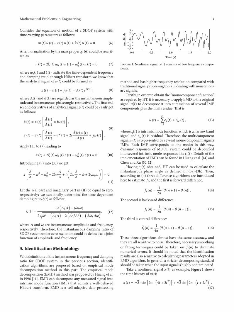
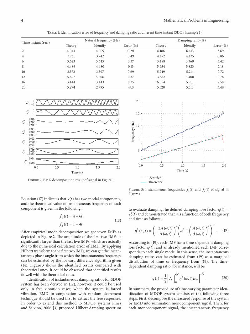
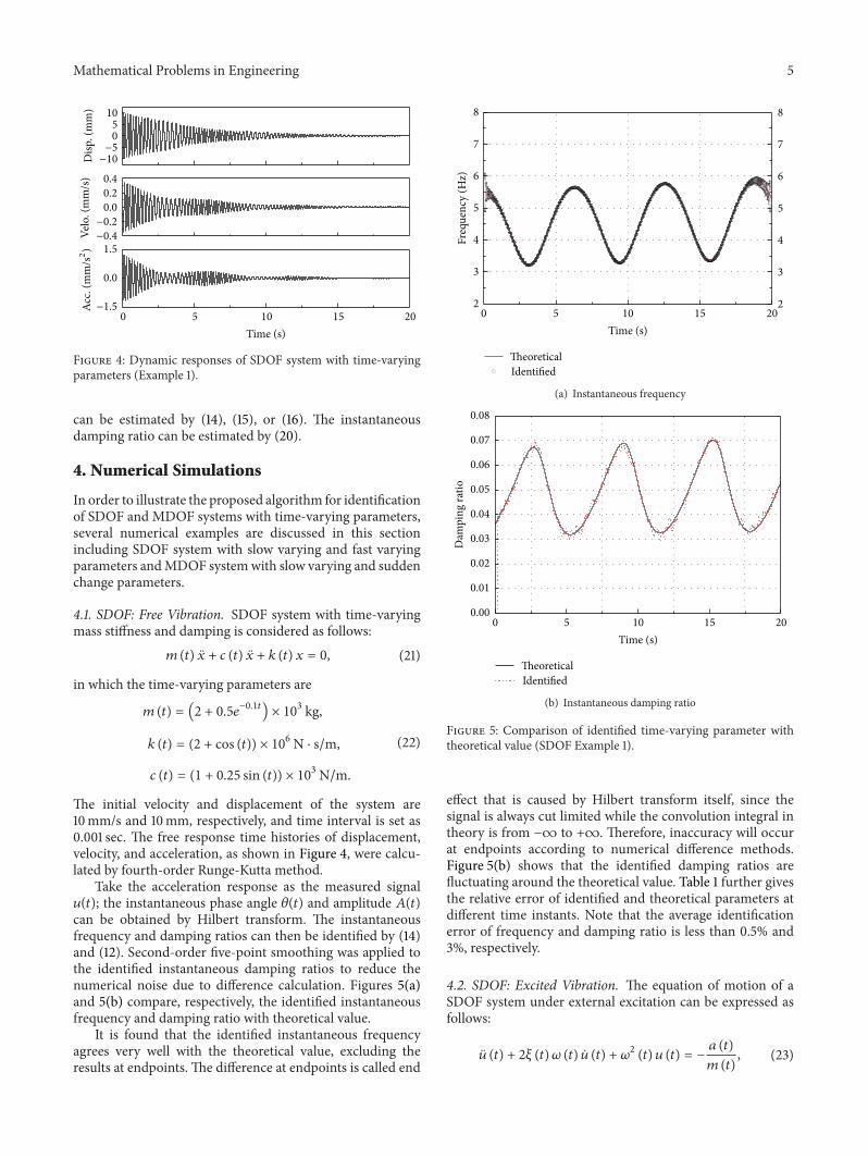
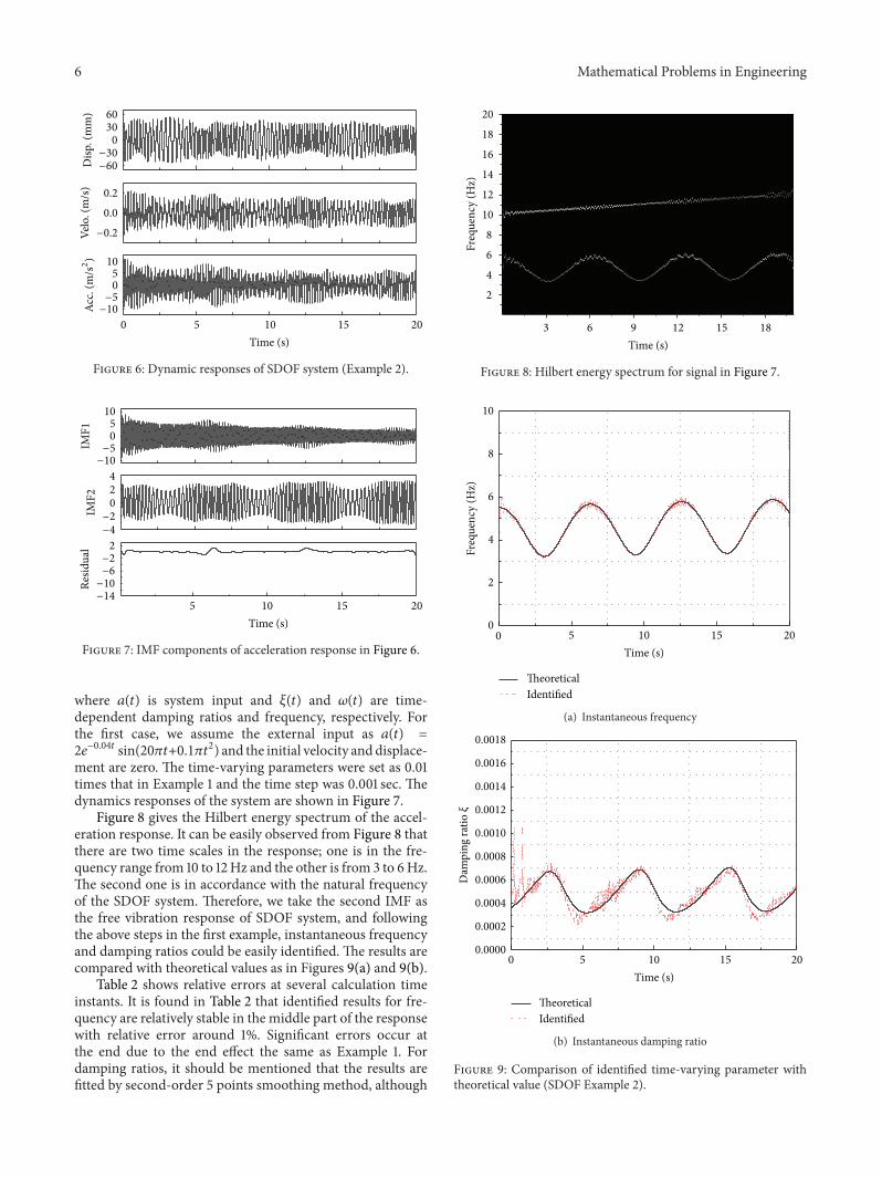
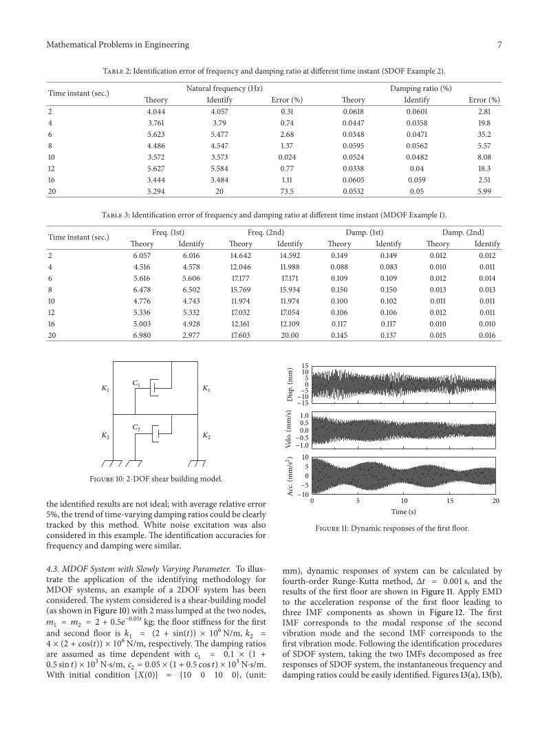
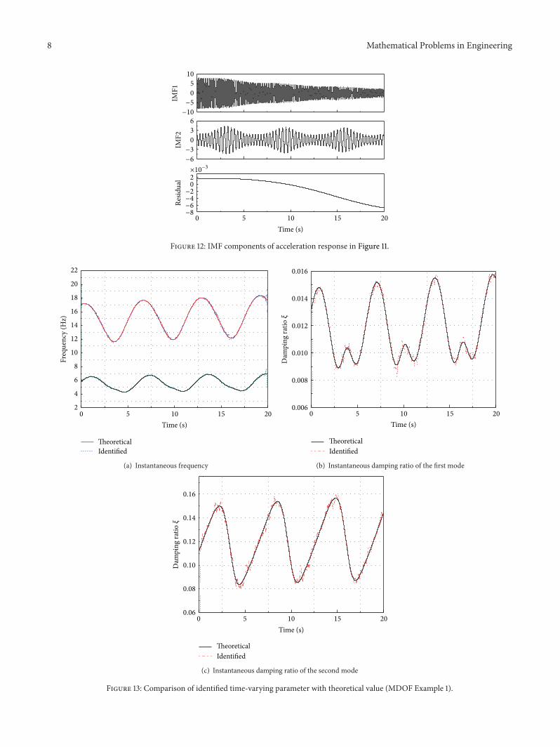
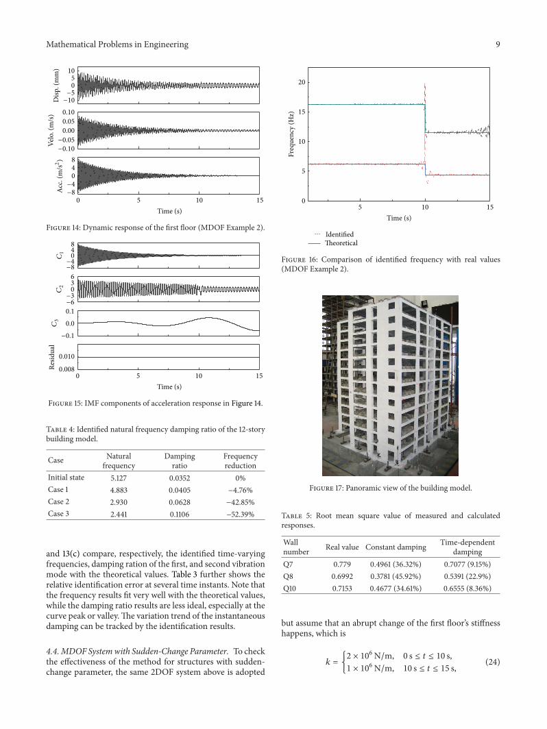
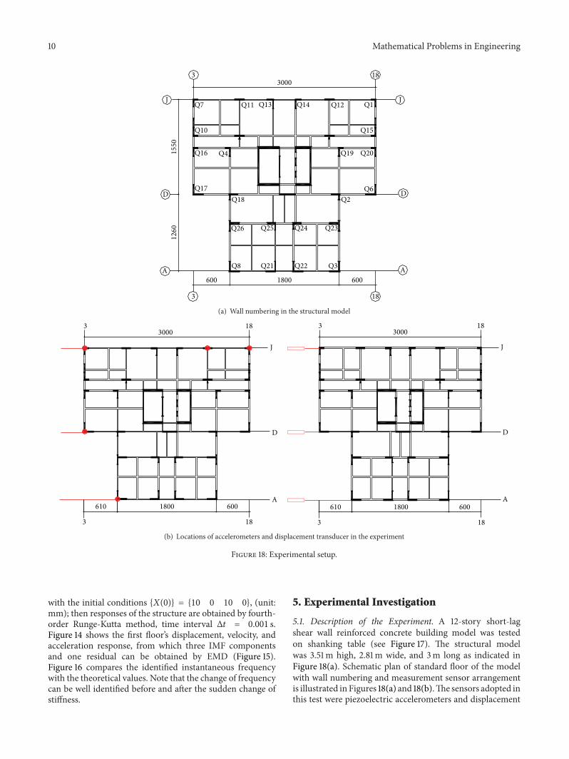
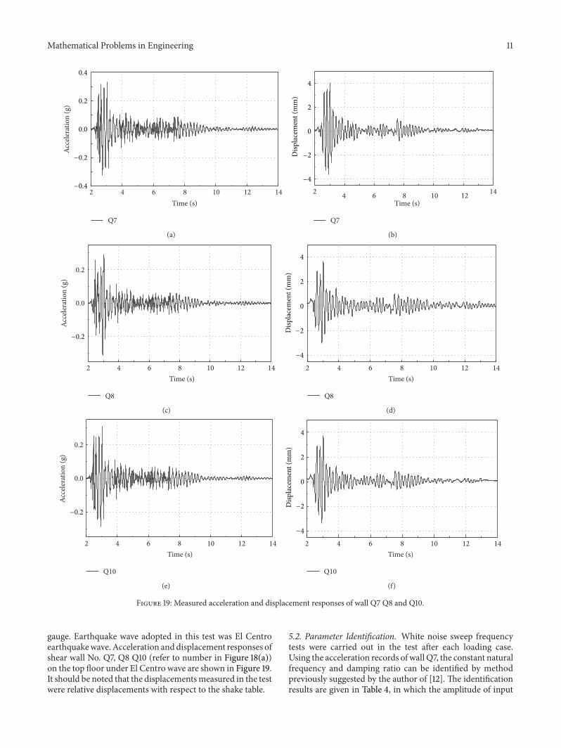
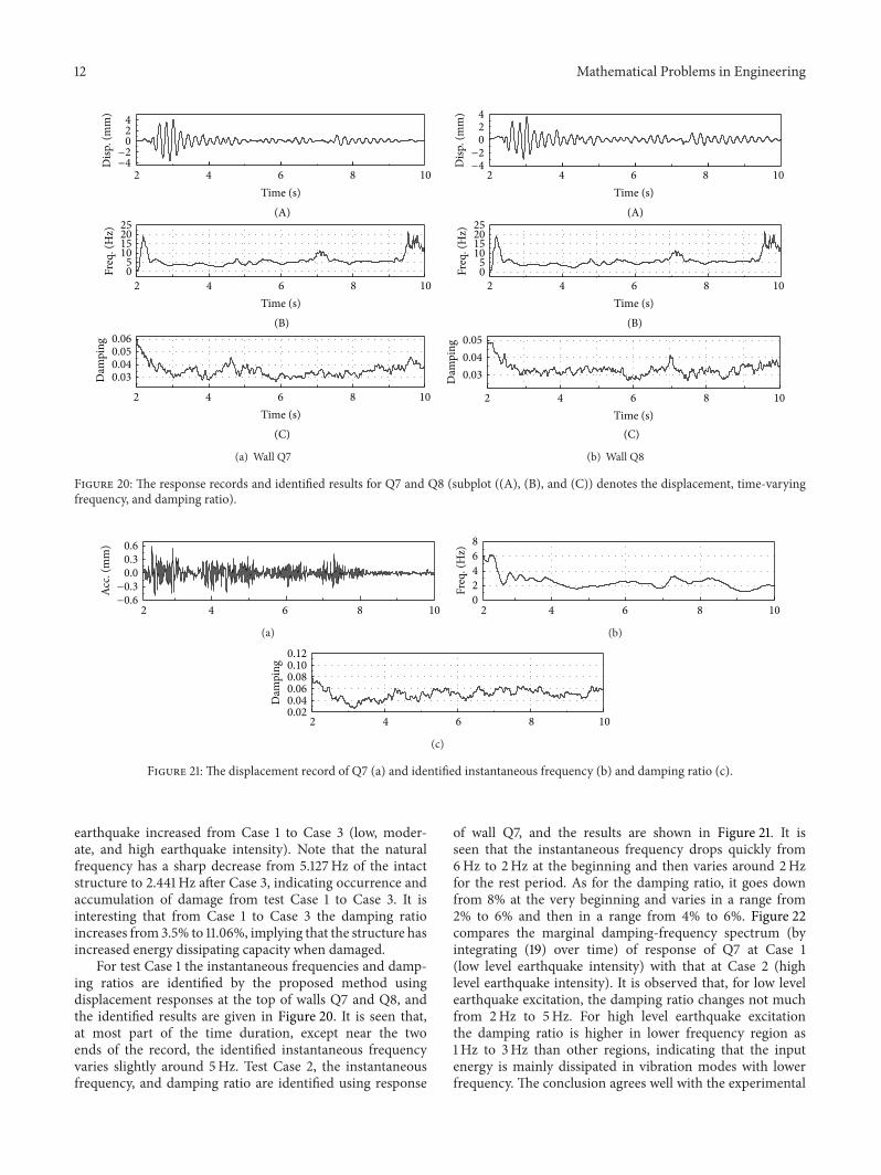
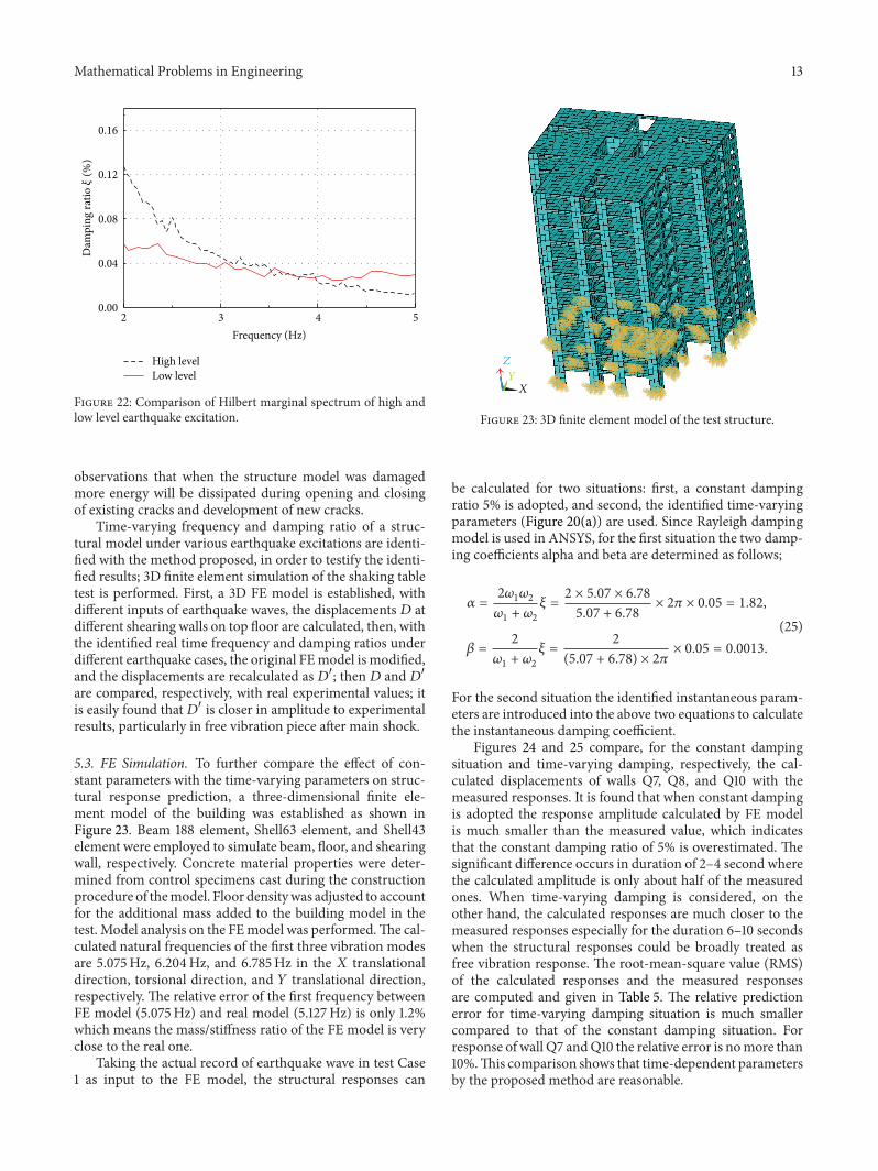
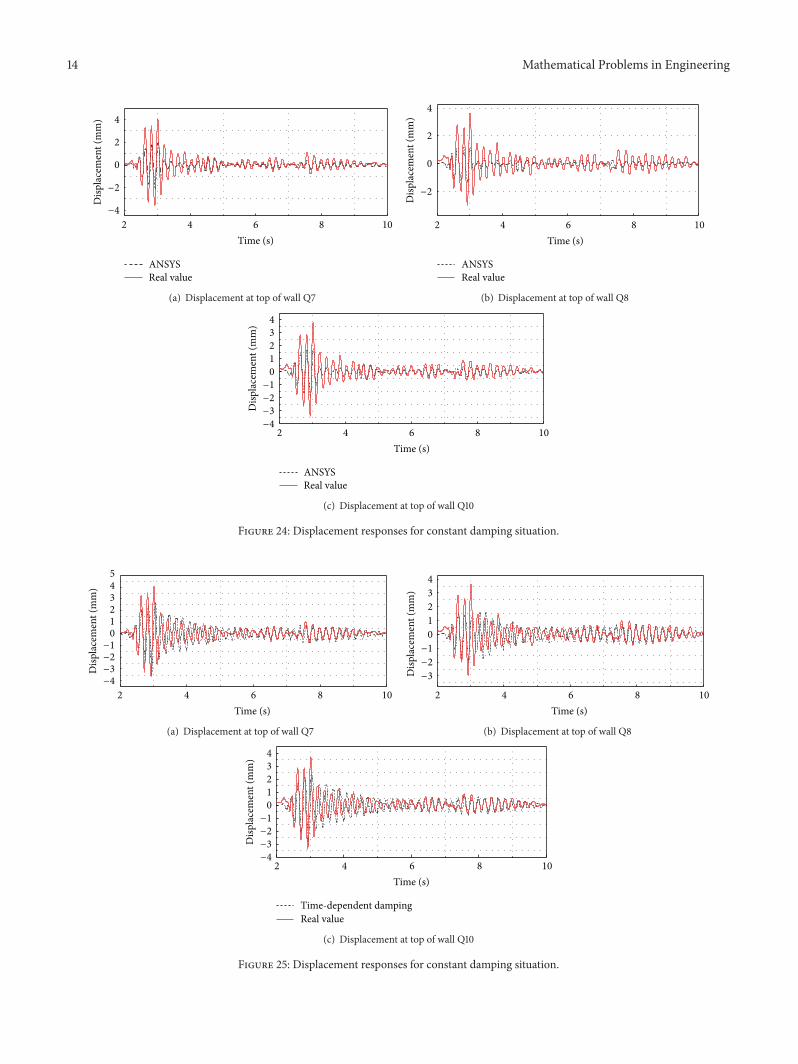
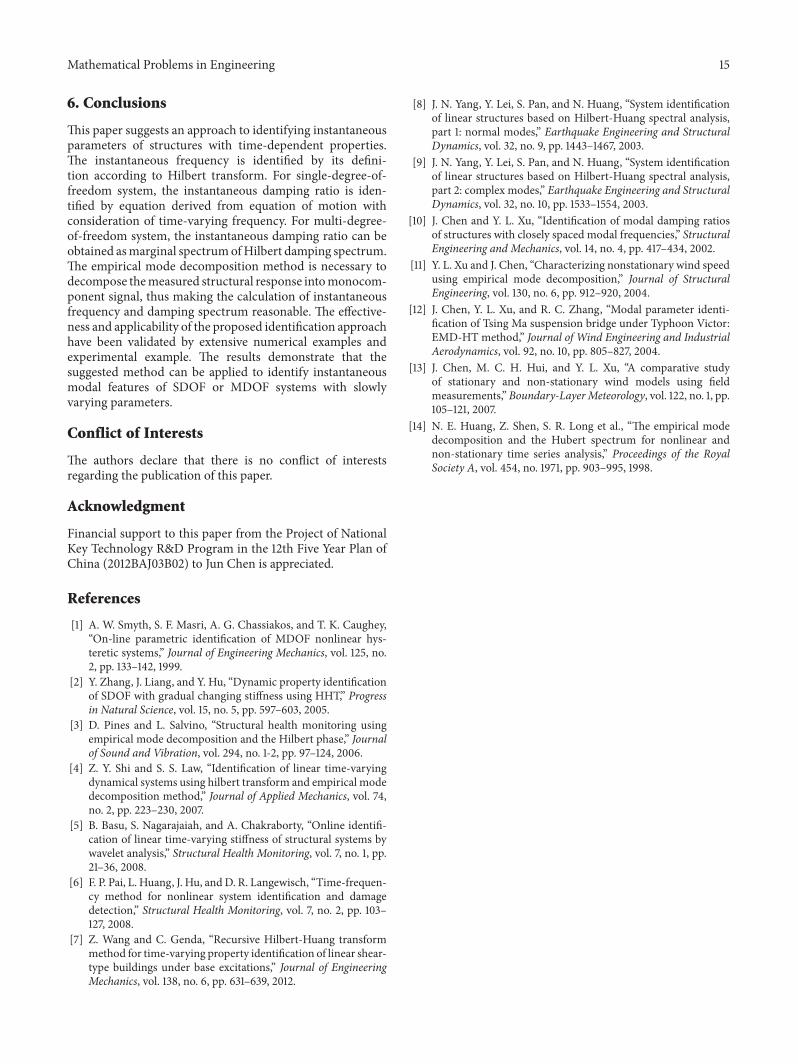