Webinar: Know Where, Why, What: Big Data’s Role In Predictive And Location Analytics
Research ArticleLPTA Location Predictive and Time Adaptive Data GatheringScheme with Mobile Sink for Wireless Sensor Networks
Chuan Zhu1 Yao Wang1 Guangjie Han1 Joel J P C Rodrigues23 and Jaime Lloret4
1 College of Internet of Things Engineering Hohai University Changzhou 213022 China2 Instituto de Telecomunicacoes University of Beira Interior 6201-001 Covilha Portugal3 University of ITMO Saint Petersburg 197101 Russia4 Integrated Management Coastal Research Institute Universidad Politecnica de Valencia 46022 Valencia Spain
Correspondence should be addressed to Guangjie Han hanguangjiegmailcom
Received 24 April 2014 Accepted 24 July 2014 Published 3 September 2014
Academic Editor Zhongmei Zhou
Copyright copy 2014 Chuan Zhu et al This is an open access article distributed under the Creative Commons Attribution Licensewhich permits unrestricted use distribution and reproduction in any medium provided the original work is properly cited
This paper exploits sinkmobility to prolong the lifetime of sensor networks while maintaining the data transmission delay relativelylow A location predictive and time adaptive data gathering scheme is proposed In this paper we introduce a sink locationprediction principle based on loose time synchronization and deduce the time-location formulas of the mobile sink Accordingto local clocks and the time-location formulas of the mobile sink nodes in the network are able to calculate the current location ofthe mobile sink accurately and route data packets timely toward the mobile sink by multihop relay Considering that data packetsgenerating from different areas may be different greatly an adaptive dwelling time adjustment method is also proposed to balanceenergy consumption among nodes in the network Simulation results show that our data gathering scheme enables data routingwith less data transmission time delay and balance energy consumption among nodes
1 Introduction
With the enormous development in the field of embeddedcomputing and wireless communication technology wirelesssensor networks (WSNs) nowadays are more applicable andpracticable than theWSNs in the past were A wireless sensornetwork is composed of hundreds or thousands of distributedsensors that monitor their interesting surroundings andreport sensed data to a static base station or sink throughmultihop relay Typical applications of WSN include targettracking environment monitoring military surveillancehealth monitoring natural disasters forecasting and so forth[1ndash3] Sensors with limited energy are usually left unattendedafter the initial deployment And the environments of thedeployment area are often harsh and involve obstacles whichmakes sensors battery replacement infeasible Hence it isexpected to minimize and balance energy consumption ofsensors to prolong the network lifetime It has been provedthat in a static network the sensors deployed near the sinkexhaust their energy faster than those far apart due to theirheavy overhead of relaying messages and this is the so
called ldquohot-spotrdquo problem [4] In addition node failure ormalfunction may cause energy holes in the deployed areaand the network connectivity and coverage around the sinkmay not be guaranteed [5] Therefore unbalanced energyconsumption causes network performance to be degradedand network lifetime shortened
Recently various new strategies that use mobilityattributes of elements in WSNs have been investigated toreduce and balance energy consumption of sensors [6 7] Inthis paper we consider utilizing a mobile sink to proactivelycollect data generating from sensor network and thisstrategy is also favored by many researchers [8ndash10] Whenthe sink moves in the network the role of the ldquohot-spotrdquorotates among sensors [11] resulting in balanced energyconsumption among nodes The effectiveness of usingmobile sinks to gather data has been demonstrated both bytheoretical analysis and experimental study [12ndash15]
Generally when a mobile sink is adopted to collect dataall over the network it should consider the following tworequirements
Hindawi Publishing Corporatione Scientific World JournalVolume 2014 Article ID 476253 13 pageshttpdxdoiorg1011552014476253
2 The Scientific World Journal
(i) Low Data Delivery Latency Cheap sensors deployedin the monitored environment are often equippedwith limited resources that is energy memory spaceand so forth And the speed of a mobile sink isrelatively slow compared with the speed of wirelesswave These features may cause a long data trans-mission delay which will lead to sensor nodes outof memory and packets lost Therefore reducingdata delivery latency is necessary especially in time-sensitive applications
(ii) Less Control Message Overhead When a sink movesit must broadcast its current location to the sensornodes in the network repeatedly The broadcastingamong sensors consumes a large amount of energyresulting in rapid energy depletion Due to the lim-itation and the preciousness of the energy resourceit is particularly important to reduce the energyconsumption of the control overhead among sensornodes
In this paper we propose location predictive and timeadaptive (LPTA) data gathering scheme with mobile sinkfor wireless sensor networks which extends the lifetime ofthe network with less sinkrsquos location updating overhead andreduces the data transmission latency The data gatheringprocess is composed of multiple data gathering periodsEach data gathering period consists of three phases loosetime synchronization phase date collection phase and datagathering period ending declaration phase The followingprimary features make our LPTA scheme differentiated fromother existing data gathering algorithms [8 9 16]
(i) LPTA Needs No Location Updating Information for theMobile Sink Many existing data gathering algorithms forexample ALURP [8 9] need to broadcast the mobile sinklocation information during data gathering process Ourproposed scheme is based on a loose time synchronizationmechanism among sensor nodes and the mobile sinkThere-fore each node in the network is able to calculate the positionof the mobile sink based on their local clock It significantlyreduces the control messages overhead and makes the datareporting at any time possible for every sensor node
(ii) LPTA Is an Adaptive Algorithm in Terms of Sinkrsquos DwellingTime In many scenarios the deployed environments are notideal and often involve obstacles The deployment of sensornodes in such environments is nonuniform Additionally thefrequentness and number of the events of interest may bedifferent for different part of the deployment area duringdifferent periods In LPTA according to the quantity ofthe data generated from different area of the network themobile sinkrsquos dwelling time at different sojourn points canbe adjusted adaptively resulting in more efficient energyconsumption of nodes
The contributions of this paper can be summarized asfollows
(1) LPTA Utilizes Location Prediction to Reduce Data Trans-mission Delay and Location Broadcasting OverheadThe loose
time synchronization at the beginning of each data gatheringperiod and themobile sinkrsquos fixedmoving track with constantspeed make the calculation of mobile sink location possible
(2) LPTA Avoids Getting Sensor Nodes out of Memory Whenthere is data to report or relay to themobile sink sensor nodescan calculate the location ofmobile sink and send out the dataimmediatelyTherefore sensor nodes need not cache the datafor a long time and wait for the sink moving to neighboringscope
(3) LPTA Takes Obstacles into Accoun and Can Adjust theSink Dwelling Time at Sojourn Points during Data GatheringThe criteria for the time adaptation is based on the quantityof history data generated in each area When gathering datathe mobile sink will dwell longer time in the area with moredata to send than thosewith less resulting in the average relayhops decreased and the energy efficient for data transmission
As the implication of of LPTA abbreviation our LPTAmainly focuses on two strategies
(1) mobile sink location prediction
(2) dwelling time adjustment of mobile sink
During the process of data reporting from nodes to themobile sink shortest data routing protocol or other existingrouting protocols can be adopted as long as data can berelayed to the mobile sink based on location information Tosimplify our scheme and focus on the two strategies of LTPAwe use shortest path routing protocol as the data routingprotocol
The rest of this paper is organized as follows We presentrelated work in Section 2 The network model and problemstatement of our scheme are given in Section 3 Then themoving strategy of the mobile sink is presented in Section 4and the data reporting process of nodes towards the mobilesink is described in Section 5 And in Section 6 the perfor-mance of our protocol is analyzed and compared with that ofthe adaptive sink mobility scheme (Adaptive) [16] in terms ofdata transmission latency and energy consumption throughsimulations Finally the conclusion is given in Section 7
2 Related Work
Here we briefly summarize some of the related works ondata gathering mechanisms in WSNs According to themain purpose of these works the existing protocols can beclassified into three categories extension of network lifetimereduction of sinkrsquos location updating overhead and reductionof time delay of data reporting
21 Extension of Network Lifetime To alleviate the influenceof ldquohot-spotrdquo a number of research works on prolonging thelifetime of WSNs by using mobile sinks have been proposedWang et al [17] explored sinkmobility to prolong the lifetimeof sensor networks They gave a linear programming formu-lation for the joint problems of determining the movementschedule of the sink and the sojourn time at different points in
The Scientific World Journal 3
the networkTheir proposed routing scheme canwork only ina grid network topology Luo and Hubaux [15] proved that ina circle topology to achieve the maximum network lifetimea mobile sink should rotate on the periphery of the networkA joint mobility and routing strategy with a combination ofperiphery moving and round routing was proposed Thenby assuming Manhattan routing Lee et al [10] obtained thesimilar conclusion They also proposed a heuristic algorithmfor sink mobility to achieve near-optimal network lifetimeLiu et al [18] proposed a density adjustment algorithmin order to increase the network lifetime and coverage byappropriately adjusting node density A biased adaptive sinkmobility scheme (Adaptive) was proposed in [16] In order toachieve accelerated coverage of the network and fairness ofservice time of each region the sink moves probabilisticallyfavoring less visited areas and adaptively staying longer innetwork regions that tend to produce more data Adaptivebalances the energy consumption among nodes and prolongsthe network lifetimeHowever because themobile sink has totraverse all vertexes in the graph it may cause a rigorous timedelay problem in large scale networks
22 Reduction of Sinkrsquos Location Updating Overhead Sinkrsquoslocation updating may cause great energy overhead of nodesTherefore some schemes have been suggested to reducelocation updating control messages Ye et al [19] presenteda Two-Tier Data Dissemination (TTDD) protocol in whicheach data source proactively constructs a grid structureenabling mobile sinks to continuously receive data on themove by flooding queries within a local cell only The sinkconfines the destination area as it moves in order to broadcastits location information within the destination area onlyrather than to the entire network so as to reduce energyconsumption of location updating message Similarly in [8]Wang et al proposed Adaptive Local Update-based RoutingProtocol (ALURP) which uses local flooding method toeffectively update the location information of a mobile sinkHowever there is substantial overhead for sinkrsquos locationupdating especially when the sink moves at high speed Shinand Kim [9] proposed a milestone-based predictive routingprotocol that improves energy efficiency and prolongs thelifetime of networks By introducing milestone node theestimated sinkrsquos future location information is spread towardsthe nodes located in the vicinity of the recent trail of thesink by multihop relay by milestone node The neighborsof these relay nodes can update their own ldquorouting infor-mationrdquo by overhearing as a result all local nodes canacquire the latest location information of the mobile sinkThis protocol improves energy consumption and data packetdelivery ratios However it still needs substantial overheadwhen sinks change their moving direction frequently Shi etal [20] proposed an efficient data-driven routing protocolwith mobile sinks (DDRP) In order to reduce the protocoloverhead for route discovery and maintenance caused bysink mobility while keeping high packet delivery DDRPintegrates data-driven routing and randomwalk routing in itsimplementation Exploiting the broadcast feature of wirelessmedium nodes overhear the data packets transmitted by
their neighbors to learn fresh route information towards thesink When no route to the mobile sink is known randomwalk routing is adopted for data packet forwarding DDRPcan achieve lower protocol overhead and longer networklifetime Fodor and Vidacs [21] reduced communicationoverheads by proposing a restricted flooding method Routesare updated only when topology changes In [22] theauthors utilize a logical coordinate system to infer distancesand establish data reporting routing by greedily selectingthe shortest path to the destination reference It effectivelyreduces energy consumption However when changing itslocation the mobile sink still needs to reestablish logicalcoordinate system
23 Reduction of TimeDelay ofDataReporting Theintroduc-tion of mobile sink may cause serious time delay problemtherefore many researchers seek solutions to this kind ofproblems under time-sensitive application scenarios Liang etal [14] studied the network lifetime maximization problemfor time-sensitive data gathering using a mobile sink withseveral constraints such as the total travel distance andmaximum distance between the sinkrsquos two sojourning loca-tions They presented a mixed integer linear programmingsolution to this multiple-constrained problem and proposeda heuristic solution Xing et al [6] proposed a rendezvous-based approach in which a subset of nodes serve as the ren-dezvous points (RPs) that buffer data originated from sourcesand transfer to MEs when they arrive Taking data deliverydeadline into account RP-CP and RP-UG were proposed tofacilitate reliable data transfers from RPs to MEs under thecondition of significant unexpected delays in ME movementand network communication Aioffi et al [23] proposed theMinimumWiener index Spanning Tree (MWST) as a routingtopology for multiple base stations A branch and boundalgorithm for small-scale WSNs and a simulated annealingalgorithm for large-scale WSNs are designed alternativelyThe energy efficiency and packet delay attributes perfor-mance better than that of traditional minimum spanningtree
In this paper a location predictive and time adaptivedata gathering scheme with mobile sink is proposed forwireless sensor networks The trajectory of mobile sink canbe a predefined circle rectangle or other geometric shapesdepending on the deployed area and the moving velocity ofthe sink is a constant These two conditions make the mobilesink location predictable which reduces the energy overheadfor broadcasting location update messages of the mobilesink while maintaining low data transmission delay Whenreporting or forwarding data to the mobile sink sensorscalculate the location of the mobile sink based on a loosetime synchronization mechanism among sensor nodes andthe mobile sink Different from [9] in LPTA the mobile sinkneeds no location updating message to inform sensor nodesof its latest location which saves a lot of control overheadThe sink collects data from sensors only when it is dwellingat sojourn points The sink dwelling time at sojourn points isdynamically adjustable but unlike depending on local nodesdensity in [16] time adjustment method in our scheme is
4 The Scientific World Journal
based on the number of historical data generated in each areawhich is more applicable to real environments
3 Network Model and Problem Statement
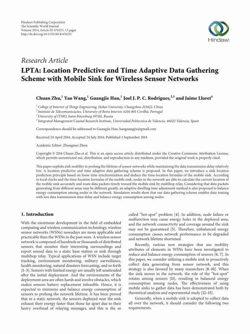
The network model is shown in Figure 1 119873 sensor nodesare deployed randomly in the network and one mobile sinkgathers data from the whole network All sensor nodesare quasi-stationary and location-aware (ie equipped withGPS-capable antennae) The mobile sink is not constrainedby energy and can move at constant velocity The wholenetwork area is a119882times119871 rectangle and the mobile sink movesalong a predefined trajectory A predefined fixed trajectory isthe base of location prediction and many researchers haveinvestigated the performance of different trajectory for datagathering protocols [10 15 24] We use a rectangle of 119908 times 119897
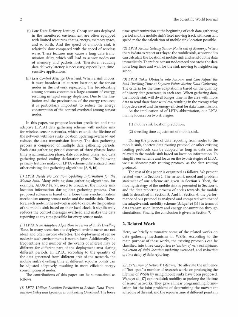
and a circle with radius 119877 as the examples of trajectories inour network as shown in Figures 1 and 2 respectively Theprediction of the location of mobile sink based on these twotrajectories is simple and effective
As described in Section 1 the frequentness and thenumber of the events of interest may be different in differentpart of the deployment area And the network is deployed intotwo-dimensional Cartesian coordinate system To simplifythe related formulas and expressions focus on the corealgorithm of LPTArsquos dwelling time adjustment and make iteasily understood we divide the network into four quadrantsand its center is denoted as origin point 119874 The mobile sinkturns off its radio transceiver while moving between twosojourn points and collects data from sensors only when itis dwelling at sojourn points The number of sojourn points119899 is a multiple of four and they are evenly distributed onthe trajectory Because the dwelling time of the mobile sinkis adjusted based on the data generation portion of differentregion rather than different sojourn point the number ofsojourn points has no effect on the overhead of controlmessage and is only used for mobile gathering data in apredictive discrete manner An anticlockwise rule is usedto determine which quadrant a sojourn point belongs tofor example point 119860 belongs to quadrant I as shown inFigure 1 In Section 6 the simulation results under differentsinkrsquosmoving trajectory show that when sinkmoves along therectangle trajectory there is a better performance Thereforethe location formulas of the mobile sink in our paper will begiven based on a rectangle trajectory and other conditionssuch as circle trajectory can be acquired in a similar way
Sensor nodes are able to communicate with the mobilesink by multihop relay The nodes that can communicatedirectly with the sink within their communication radius 119903are one-hop neighbors of the mobile sink For the sake ofconvenience the main symbols used in this paper are listedin Notations Section
There are two core problems to be solved in this paperThefirst one is the moving strategy of the mobile sink It includesthe behavior of the mobile sink when the sink moves alongthe predefined trajectory and the dwelling time adjustingmethod in each quadrant As illustrated in Figure 1 theremaybe obstacles in the monitoring area for example pools or
A
BC
E
G HF
O
D
Sensor
Packets transmitted from sensor to sink
Mobile sinkSojourn point Obstacle
II I
IVIII
D998400
Figure 1 Network model of rectangle trajectory
O A
B
C
D
E
G
HF
D998400
II I
IVIII
Sensor
Packets transmitted from sensor to sink
Mobile sinkSojourn point Obstacle
Figure 2 Network model of circle trajectory
swamps we assume nodes deployed in these area are disabledto monitor the surroundings which will cause the differenceof data amount generating from each quadrant Thereforeit is necessary to adjust the dwelling time of mobile sinkto reside longer in the quadrant which generates more datapackets The mobile sink can be a quadcopter or an aircraftwhich is not influenced by these obstacles when movingalong the trajectory The second one is the data routingmethod for sensor nodes reporting data towards the mobilesink Multihop relay communication method among nodesis adopted as shown in Figure 1 Source node uploads data
The Scientific World Journal 5
packets towards the mobile sink by multihop relay Both ofthem will be stated in detail in the following section
4 Sink Moving Strategy
In this section we describe the data gathering process ofmobile sink and introduce the dwelling time adaptive criteriaThe data gathering process is periodically carried out by themobile sink During the periodical data gathering processthe mobile sink circles along the trajectory stops at a sojournpoint to collect sensed data and then moves to the nextsojourn point To simplify our data gathering scheme wedivide the whole data gathering process into several timeintervals each of which is corresponding to a data gatheringperiod (DGP) The mobile sink circles along the trajectoryover and over in one data gathering period and we furtherdivide one data gathering period into multiple data gatheringcircles (DGPs) The detailed definition of data gatheringperiod and data gathering circle are as follows
(i) Data Gathering Period (DGP) A DGP is defined asthe process from the beginning of the sink enteringthe network to its leaving the network During oneDGP the mobile sink carries out the data gatheringalgorithm which includes loose time synchronizationphase time adaptive data collection phase and DGPending declaration phase One DGP is composed ofmultiple DGCs
(ii) Data Gathering Circle (DGC) A DGC refers to theprocess of the sink moving along the trajectoryand backing to the initial point For example thesink starts from sojourn point 119860 moves along thetrajectory passes through sojourn points from119861 to119867and comes back to point119860 again as shown in Figure 1This process is a DGC
The number of DGCs contained in one DGP depends onthe application requirements and is limited by the availableenergy carried by the mobile sink The higher the valuethe better it is Because at the beginning and the endingof one DGP the mobile sink needs to broadcast a HELLOmessage and aBYEmessage respectively whichwill consumethe energy of nodes Considering realistic situation it is set10 in our simulation Additionally as the relevant formulasof sinkrsquos location is related to sinkrsquos moving trajectory weonly give the formulas hereinafter according to the rectanglemoving trajectory similarmethods can be used to acquire theexpression of other shapes
41 Loose Time Synchronization The mobile sink as wellas every node in the network owns its own clock At thebeginning of one DGP the mobile sink broadcasts a timesynchronization message HELLO to achieve loose timesynchronization among the mobile sink and all nodes inthe network Based on this synchronization every node inthe network can calculate the location of the mobile sinkaccording to its local time information when uploading datapackets to the mobile sink
The loose time synchronization phase is the first phaseduring oneDGPWhen entering into the network themobilesink broadcasts aHELLOmessage to the whole networkTheHELLOmessage consists of the starting location information119878(119909 119910) current time 119905
0 the moving velocity 119881 of the mobile
sink the number of sojourn points 119899 on the trajectory thedwelling time at each sojourn point in quadrant 119894 (119894 isin
1 2 3 4) during the first DGC 119879119904(119894 1) and the width and
length of rectangle trajectory119908 and 119897 Every node changes itsclock to 119905
0when it receives the HELLO message for the first
time and then retransmits this message to its neighbors Notethat the parameters 119879
119904(119894 1) in the HELLO message are equal
to each other that is 119879119904(1 1) = 119879
119904(2 1) = 119879
119904(3 1) = 119879
119904(4 1) =
119879119904After the network achieved loose time synchronization
the mobile sink starts to collect data packets from thenetwork The time for loose time synchronization can beignored since it is quite small compared with the time for oneDGP
42 Time Adaptive Data Collection During the time adap-tive data collection phase the dwelling time is adjusteddynamically In some application scenarios there may existobstacles in the network area hence the data generated fromeach quadrant can be different greatly According to thevariation degree of 119875data(119894 119896 minus 1) and 119875data(119894 119896) the dwellingtime 119879
119904(119894 119896 + 1) in the (119896 + 1)th DGC at sojourn points is
adjusted dynamically In this way the energy consumption ofentire network can be further balanced
As the data packets in each quadrant are generated in arandom manner and transmitted by multihop relay to themobile sink the routing path for these packets generatedin quadrant 119894 will be longer than those in quadrant 119895 (119894 =
119895) where the mobile sink locates therefore the former willconsume much more energy than the latter To reduce theenergy consumption caused by long distance data packetsrouting after finishing each DGC the mobile sink statisticsthe number of packets received from each quadrant and thencalculates the proportion of these packets to the entire net-work data packets 119875data1 119875data2 119875data3 and 119875data4 accordinglyDepending on these proportions the dwelling time of themobile sink at sojourn points in each quadrant is adjusteddynamically which makes the energy consumption in thenetwork more balanced and the network lifetime extended
The principle of adjusting the dwelling time 119879119904(119894 119896 + 1) in
the (119896 + 1)th DGC is described in detail as followsIn order to distinguish the quadrant in which a data
packet is generated source nodes append a 2-bit quadrantinformation to the head of the data packet before sending itto its next hop The quadrant information can be calculatedbased on the sensor node location loc(119909
119894 119910119894) relative to the
origin point 119874rsquos location information Note that only thesource nodes need to add their own quadrant information tothe head of the data packets
During one DGP the mobile sink calculates the (119896 +
1)th DGCrsquos dwelling time in each quadrant according to theproportions 119875data1 119875data2 119875data3 and 119875data4 in the (119896 minus 1)thDGC and the proportions in the 119896th DGC When the value
6 The Scientific World Journal
119875change(119896 119896 minus 1) is greater than the threshold value 119879ℎ the
dwelling time in corresponding quadrant will be adjustedas 119879119904(119894 119896 + 1) = 4119875data119894119879119904 The value of 119875change(119896 119896 minus 1) is
calculated according to the following formula
119875change (119896 119896 minus 1)
= radic
4
sum
119894=1
(119875data (119894 119896) minus 119875data (119894 119896 minus 1))2
(1)
119875change (119896 119896 minus 1) represents the variation degree of datageneration proportion in different quadrant between twoadjacent DGC When this value is greater than the threshold119879ℎ it means that the quantity of data packets generated in
each quadrant has changed significantly and the dwellingtime needs to be adjusted Under this circumstance themobile sink will broadcast a UPDATE message to all nodesin the network which includes the adjusted dwelling time ineach quadrant 119879
119904(119894 119896 + 1) Otherwise there is no necessity
to modify the dwelling time and the mobile sink maintainsthe dwelling time in each quadrant the same as the previousDGC
43 DGP Ending Declaration DPG ending declaration phaseis the last phase in oneDGP At the beginning of the last DGCof one DGP the mobile sink broadcasts a BYE message toall nodes in the network The broadcasting of BYE messagemeans that the current DGP is coming to an end and themobile sink will stop gathering data and leave the networkThe BYE message consists of the time 119879bl which is the timeinterval between current time and the mobile sink finishingcurrent DGP Instead of routing the data to the mobile sinkwhen receiving BYE messages nodes will buffer the datasensed from surroundings after time 119879bl
119879bl = 119899119879119904 +2 (119908 + 119897)
119881minus 2119879syn (2)
119879syn is the time needed for the network to achieve loose timesynchronization and as to 119879syn there is
119879syn ≪ 119899119879119904+2 (119908 + 119897)
119881 (3)
Therefore 119879syn has little effect on 119879bl and can be ignored inpractical applications
5 Data Reporting Process
In the network source nodes transmit data packets to themobile sink by multiple hops The principle of selecting nexthop is to make the path between a source node and themobile sink approximately shortest When nodes have datato report or relay they need to calculate the mobile sinkscurrent location based on their own clocks which have beenloosely synchronized to the mobile sink and then chooseone of its neighbors as the next hop Using other existingrouting protocols for data routing is also feasible Our schemefocuses on sinkrsquos location prediction and its dwelling time
A
lwlw2 w2d(t)
AHFDB
Figure 3 Mapping model of rectangle trajectory
adjustment If there exists the concave obstacle which mayresult in data reporting failed obstacle avoidance routingprotocols can be adopted to relay the data packets to themobile sink
The time step119879step is the time interval formoving betweentwo adjacent sojourn points It is calculated by the followingformula
119879step =2 (119908 + 119897)
119899119881 (4)
During the loose time synchronization phase the mobilesink broadcasts a HELLO message to achieve loose timesynchronization among all the nodes in the network Theparameter 119879
119904(119894 1) in the HELLO message is equal to each
other that is 119879119904(1 1) = 119879
119904(2 1) = 119879
119904(3 1) = 119879
119904(4 1) = 119879
119904 119879119904
is a constant value and keeps unchanging during a DGPTo determine the location of the mobile sink at time 119905
in this paper we have the moving trajectory of the mobilesink map to a line model In the model the starting locationof a DGP is chosen as the reference location for examplepoint119860 in Figure 3 Corresponding to the rectangle trajectoryillustrated in Figure 1 the line model is shown in Figure 3 inwhich the 119889(119905) is the distance from the reference location 119860to the current location of mobile sink in the present DGC
The moving time of the mobile sink in current DGC isdenoted as 119879
119901 which is calculated by the following formula
119879119901= [
119905 minus 1199050
119899 (119879step + 119879119904)] (5)
Based on loose time synchronization the location of themobile sink can be calculated by the following formulas
(1) If
0 le 119879119901lt119899119879119904 (1 119896)
4+119908 + 119897
2119881 (6)
then
Loc (119905) =
(minus119897
2 119889 (119905)) 119889 (119905) lt
119908
2
(minus119897
2+ (119889 (119905) minus
119908
2)
119908
2) others
(7)
119889(119905) can be calculated as below
1198791=
(119879119901minus lfloor119879119901 (119879step + 119879119904 (1 119896))rfloor (119879step + 119879119904 (1 119896)))
(119879119904 (1 119896))
(8)
and if lfloor1198791rfloor = 0 then
119889 (119905) = 119881lfloor
119879119901
119879step + 119879119904 (1 119896)rfloor119879step (9)
The Scientific World Journal 7
else
119889 (119905) = 119881(119879119901minus lceil
119879119901
119879step + 119879119904 (1 119896)rceil119879119904(1 119896)) (10)
(2) If
119899119879119904(1 119896)
4+119908 + 119897
2119881
le 119879119901lt119899 (119879119904 (1 119896) + 119879119904 (2 119896))
4+2 (119908 + 119897)
2119881
(11)
then
Loc (119905) =
(minus119897
2+ (119889 (119905) minus
119908
2)
119908
2) 119889 (119905) lt
119908
2+ 119897
(119897
2119908
2minus (119889 (119905) minus 119897 minus
119908
2)) others
(12)
119889(119905) can be calculated as below
1198792= (119879119901minus119899119879119904(1 119896)
4minus119908 + 119897
2119881
minus lfloor
119879119901minus 119899119879119904 (1 119896) 4 minus (119908 + 119897) 2119881
119879step + 119879119904 (2 119896)rfloor
times (119879step + 119879119904 (2 119896)))
times (119879119904(2 119896))
minus1
(13)
and if lfloor1198792rfloor = 0 then
119889 (119905) = 119881(119908 + 119897
2119881+ lfloor
119879119901minus 119899119879119904(1 119896) 4 minus (119908 + 119897) 2119881
119879step + 119879119904 (2 119896)rfloor
times 119879step)
(14)
else
119889 (119905) = 119881(119879119901minus119899119879119904(1 119896)
4
minus lceil
119879119901minus 119899119879119904 (1 119896) 4 minus (119908 + 119897) 2119881
119879step + 119879119904 (2 119896)rceil119879119904 (2 119896))
(15)
(3) If
119899 (119879119904 (1 119896) + 119879119904 (2 119896))
4+2 (119908 + 119897)
2119881le 119879119901
lt119899 (119879119904(1 119896) + 119879
119904(2 119896) + 119879
119904(3 119896))
4+3 (119908 + 119897)
2119881
(16)
then
Loc (119905) =
(119897
2 minus119889 (119905) + 119897 + 119908) 119889 (119905) lt
3119908
2+ 119897
(119897
2minus (119889 (119905) minus 119897 minus
3119908
2) minus
119908
2) others
(17)
119889(119905) can be calculated as below
1198793= (119879119901minus119899 (119879119904 (1 119896) + 119879119904 (2 119896))
4minus2 (119908 + 119897)
2119881
minus lfloor
119879119901minus 119899 (119879
119904 (1 119896) + 119879119904 (2 119896)) 4 minus 2 (119908 + 119897) 2119881
119879step + 119879119904 (3 119896)rfloor
times (119879step + 119879119904 (3 119896)) )
times (119879119904(3 119896))
minus1
(18)
and if lfloor1198793rfloor = 0 then
119889 (119905)
= 119881(2 (119908 + 119897)
2119881
+ lfloor
119879119901minus 119899 (119879
119904(1 119896) + 119879
119904(2 119896)) 4 minus 2 (119908 + 119897) 2119881
119879step + 119879119904 (3 119896)rfloor
times 119879step)
(19)
else
119889 (119905)
= 119881(119879119901minus119899 (119879119904(1 119896) + 119879
119904(2 119896))
4
minus lceil
119879119901minus 119899 (119879
119904(1 119896) + 119879
119904(2 119896)) 4 minus 2 (119908 + 119897) 2119881
119879step + 119879119904 (3 119896)rceil
times 119879119904(3 119896) )
(20)
(4) If
119899 (119879119904(1 119896) + 119879
119904(2 119896) + 119879
119904(3 119896))
4+3 (119908 + 119897)
2119881
le 119879119901lt119899 (119879119904(1 119896) + 119879
119904(2 119896) + 119879
119904(3 119896) + 119879
119904(4 119896))
4
+4 (119908 + 119897)
2119881
(21)
8 The Scientific World Journal
then
Loc (119905) =
(119897
2minus (119889 (119905) minus 119897 minus
3119908
2) minus
119908
2)
119889 (119905) lt3119908
2+ 2119897
(minus119897
2 minus119908
2+ 119889 (119905) minus 2119897 minus
3119908
2)
others
(22)
119889(119905) can be calculated as below
1198794= (119879119901minus119899 (119879119904(1 119896) + 119879
119904(2 119896) + 119879
119904(3 119896))
4minus3 (119908 + 119897)
2119881
minus lfloor(119879119901minus119899 (119879119904(1 119896) + 119879
119904(2 119896) + 119879
119904(3 119896))
4
minus3 (119908 + 119897)
2119881) times (119879step + 119879119904 (4 119896))
minus1
rfloor
times (119879step + 119879119904 (4 119896)) )
times (119879119904 (4 119896))
minus1
(23)
and if lfloor1198794rfloor = 0 then
119889 (119905) = 119881(3 (119908 + 119897)
2119881
+ lfloor(119879119901minus119899 (119879119904 (1 119896) + 119879119904 (2 119896) + 119879119904 (3 119896))
4
minus3 (119908 + 119897)
2119881) times (119879step + 119879119904 (4 119896))
minus1
rfloor
times 119879step)
(24)
else
119889 (119905) = 119881(119879119901 minus119899 (119879119904 (1 119896) + 119879119904 (2 119896) + 119879119904 (3 119896))
4
minus lceil(119879119901minus119899 (119879119904 (1 119896) + 119879119904 (2 119896) + 119879119904 (3 119896))
4
minus3 (119908 + 119897)
2119881) times (119879step + 119879119904 (4 119896))
minus1
rceil
times 119879119904(4 119896) )
(25)
We define lfloor119909rfloor as the largest integer no more than 119909 lceil119909rceilas the smallest integer no less than 119909 and [11990911199092] as the
reminder of 1199091 divided by 1199092 To keep the formula as simpleas possible we require the starting point of data gatheringto be on the intersection of 119909 axis or 119910 axis Without loss ofgenerality we choose the location 119860 as shown in Figure 1 asthe starting point and deduce a series of formulas above
As described in Section 3 the moving trajectory can bea rectangle or circle When the sinkrsquos moving trajectory is acircle the time-location formulas can be acquired in a similarwayThe difference is that themoving trajectory of themobilesink is mapped into a polar coordinate system because ofcalculation convenience Figure 4 is a model of polar systemassuming the mobile sink starts its data gathering processfrom point 119860 at time 119905
0and reaches point 119861 at time 119905 the
arc length of_119860119861 is 119877120579 (0 le 120579 lt 2120587) When the sink moves
at speed 119881 in the network there is 119881(119905 minus 1199050) = 119877120579 The
corresponding polar coordinate of point 119861 is (119877 120579)Similar to rectangle trajectory based on loose time syn-
chronization the location of the mobile sink can be acquiredaccurately when the trajectory is a circle For example whenthe mobile sink locates at the first quadrant then 119879
119901meets
0 le 119879119901lt (1198994)119879
119904(1 119896) + 21205871198774119881 and the polar angle of the
sink is calculated by the following formulasIf
119879119901minus lceil119879119901 (119879step + 119879119904 (1 119896))rceil (119879step + 119879119904 (1 119896))
119879119904(1 119896)
rceil = 0 (26)
then
120579 =2120587
119899lceil
119879119901
119879step + 119879119904 (1 119896)rceil (27)
else
120579 =119881
119877(119879119901minus lceil
119879119901
119879step + 119879119904 (1 119896)rceil119879119904(1 119896)) (28)
When the sink locates at other quadrants the correspondinglocation information can be obtained in a similar manner
According to the calculated location information sourcenodes upload their sensed data to the mobile sink by multi-hop communication When events occur in the monitoringarea the sensors outside the communication range of themobile sink route data packets to their next hop directly It isunnecessary to judge the current state of themobile sink thatis moving between sojourn points or gathering data packetsat a sojourn pointOnly the neighbor nodes of themobile sinkneed to judge the state of the mobile sink If the mobile sinkis moving between sojourn points the neighbor nodes haveto wait for a period of time 119879
119908119897until the former arrives at its
next sojourn point Otherwise they transmit the data packetto themobile sink directly For instance as shown in Figure 1we assume the current location of the mobile sink is point119863if the events occur in quadrant III then data packets can berouted along the shortest routing path to point 119863 When thedata packets reach the neighbor node of the mobile sink itwill judge the state of mobile sink according to its local timeclock If the time of the nodemeets 119905
0+119896(119879step+119879119904(119894 119896)) lt 119905 lt
1199050+119896(119879step+119879119904(119894 119896))+119879119904(119894 119896) whichmeans themobile sink is
The Scientific World Journal 9
AO
120579
B(R 120579)
Figure 4 The model of polar system
still gathering data at the sojourn point119863 then this one-hopneighbor node of the sink transmits the data packets directlyto the mobile sink otherwise for example the sink is nowlocated at 1198631015840 it needs to wait time 119879
119908119897and then transmit the
data packet to the mobile sink The time 119879119908119897
is calculated bythe following formula
119879119908119897= 1199050+ (119896 + 1) (119879step + 119879119904 (119894 119896)) minus 119905 (29)
During routing data packets to the mobile sink hop-by-hop acknowledgement mechanism is applied to ensure thedata transmission rate that is if the receiver Node2 gets thedata packets from sender Node1 it will reply with an ACKmessage toNode1 IfNode1 does not receive theACK messagefrom its next hop nodeNode2within time119879Node1 considersthat the packet transmission is failed and will cache the datapackets and wait for a random time and then retransmit thepackets to its next hop again We assume that 119879 is equal tothe propagation time of a packet between two farthest nodesof the network
6 Performance Evaluation
In this section we evaluate the performance of our schemethrough extensive simulations In addition to the proposedscheme we implemented the Adaptive [16] for comparisonThe reason is that Adaptive is also a discrete data gatheringprotocol Besides the mobile sink in Adaptive dwells atsojourn points on the predefined trajectory for data collec-tion and the dwelling time is dynamically adjusted Twoperformance metrics energy consumption and data deliverylatency are investigated Energy consumption is the averageenergy that is consumed by nodes during one DGP And datadelivery latency is the time interval from a message creationto the mobile sink receiving it
61 Simulation Environment We implement our proposedscheme in MatLab In our simulation the deployment areahas a 500m times 500m square sensing field and sensor nodesare randomly deployed in the network that is area length 119871equals its width 119882 The communication range of the nodesand the mobile sink is set to 60m The mobile sink movesalong the predefined trajectory for 10 circles in every DGP
and in every DGC 5 of sensor nodes act as source nodeswhich send messages toward the mobile sink continuallywhen the sink is dwelling at sojourn points
Different simulation environments with varying sinkmoving trajectory number of nodes 119873 and mobile sinkspeed 119881 are studied We set the trajectory as circle andrectangle the length of side or radius of trajectory is setas 1198714 1198712 31198714 and 119871 And we varied 119873 from 800 to1200 119881 from 4ms to 20ms Several groups of simulationexperiments are carried out The threshold of adjustingdwelling time119879
ℎis set as 0 025 05 075 and 1119879
ℎ= 0means
the dwelling time of themobile sink needs to be changed if theproportion of packets amount quantity generated from everyquadrant is not exactly the same as previous DGC while119879ℎ= 1 means the dwelling time keeps unchanging during
one DGP
62 Simulation Results with Varying Sink Moving TrajectoryNow we discuss the influence of sink moving trajectory onnetwork performance We compare two scenarios of thetrajectory they are rectangle and circle and the mobile sinkmoves along the predefined trajectory for one DGP Thesimulation results are shown in Figures 5 6 7 and 8
Comparing Figures 5 and 7 with Figures 6 and 8respectively it is noticed that the energy consumption ofnodes is lower when the moving trajectory is rectangle thanthat of circle when the deployment area is rectangle Thesharp of sinkrsquos moving trajectory has influence on energyconsumption of nodes even if the path is predefined In thefollowing simulation the moving trajectory of the mobilesink is rectangular which is similar to network deploymentarea
As shown in Figures 7 and 8 the energy consumptionis the lowest while mobile sink moves along the track with1198714 and 31198714 length of side or radius It is different fromthe theory proposed in [15] that peripheral movement isthe best strategy because the ideal load-balanced routing ishard to satisfy Under the condition of a certain trajectorythere is an outstanding performance when 119879
ℎis less than
1 this is because the dynamic adjustment of dwelling timeis beneficial to the performance of network Besides when119879ℎ= 075 as shown in Figure 5 the energy consumption
of control message is very low This is because there is anappropriate tradeoff between the control overhead and thebalanced energy consumption among different quadrantswhen 119879
ℎ= 075 In contrast the dwelling time adjustment
frequency is too high when 119879ℎ= 0 resulting in much energy
overhead When 119879ℎ= 1 the energy consumption of control
message equals 0 which means there is no dwelling timeadjustment and the energy consumption among nodes is notwell balanced
63 Simulation Results with Varying Number of Sensor NodesNowwe discuss the performance of our scheme by setting thenumber of sensor nodes 119873 varying from 800 to 1000 whenthe moving trajectory is rectangle The simulation results areshown in Figures 9 and 10
10 The Scientific World Journal
0000225
0000200
0000175
0000150
0000125
0000100
0000075
0000050
0000025
0000000
18 28 38 48Sinkrsquos moving trajectory (L)
Ener
gy co
nsum
ptio
n of
cont
rol m
essa
ge (J
)
0-circle025-circle05-circle
075-circle1-circle
Figure 5 Energy consumption of control message with circletrajectory
0000225
0000200
0000175
0000150
0000125
0000100
0000075
0000050
0000025
0000000Ener
gy co
nsum
ptio
n of
cont
rol m
essa
ge (J
)
18 28 38 48Sinkrsquos moving trajectory (L)
0-rec025-rec05 rec
075 rec1-rec
Figure 6 Energy consumption of control message with rectangletrajectory
As illustrated in Figure 10 the energy consumption ofnodes decreases first with increased number of nodes andthen increases when 119873 is more than 1000 It is becausewith the increase of 119873 the number of selectable next hopneighbors increases as a result the hop distance and therouting path between the mobile sink and source nodesare improved which results in less energy consumption forrelaying the same quantity of data packets When 119873 is morethan 1000 the increase of the number of source nodes causesmore packets generating in the network which results inmore energy consumption of nodes when 119873 increases Theperformance is outstanding compared to the others when 119879
ℎ
is 075 and the reason is the same as explained in Section 62
0062500600
00575
00550
00525
00500
00475
00450
00425
00400
00375
Ener
gy co
nsum
ptio
n of
nod
es (J
)
18 28 38 48Sinkrsquos moving trajectory (L)
0-circle025-circle05-circle
075-circle1-circle
Figure 7 Energy consumption of nodes with circle trajectory
00625
00600
00575
00550
00525
00500
00475
00450
00425
00400
00375Ener
gy co
nsum
ptio
n of
nod
es (J
)
18 28 38 48Sinkrsquos moving trajectory (L)
0-rec025-rec05 rec
075 rec1-rec
Figure 8 Energy consumption of nodes with rectangle trajectory
64 Simulation Results with Varying Sink Speed Now weevaluate the network performance when sinkrsquos moving speed119881 varies from 4ms to 20ms The results are shown inFigures 11 and 12
It is noticed that as the mobile sink speed goes upthe energy consumption decreases This is because with theincrease of sink speed the time the mobile sink spendingfor moving between two adjacent sojourn points decreasesand the mobile sink can receive the data packets timely fromsensor nodes This results in less energy consumed
65 Simulation Results of Data TransmissionDelay and EnergyConsumption We simulated our proposed scheme as well asthe adaptive algorithm and constant algorithm described inthe adaptive sink mobility scheme proposed by Kinalis et al[16] to evaluate the performance of data delivery latency andenergy consumption by varying sinkrsquos moving speed
The Scientific World Journal 11
0000200
0000175
0000150
0000125
0000100
0000075
0000050
0000025
0000000Ener
gy co
nsum
ptio
n of
cont
rol m
essa
ge (J
)
800 900 1000 1100 1200
Number of nodes
0-rec025-rec05 rec
075 rec1-rec
Figure 9 Energy consumption of control message under varyingnumber of nodes
800 900 1000 1100 1200
Number of nodes
0-rec025-rec05 rec
075 rec1-rec
0050
0048
0046
0044
0042
0040
Ener
gy co
nsum
ptio
n of
nod
es (J
)
Figure 10 Energy consumption of nodes under varying number ofnodes
The results are shown in Figure 13 Our LPTA schemeoutperforms the Adaptive scheme in the attribute of latencyThe reason is that in LPTA the latency is mainly causedby the mobile sink turning off its communication modelwhen moving between two adjacent sojourn points But inadaptive and constant algorithms the sink has to traverseall vertexes which results in large time delay Besides theincrease of speed is beneficial for our LPTA It is because thetime needed decreases for moving the same distance withhigher moving speed Hence the data transmission delaysignificantly reduced with the increase of sink speed
Figure 14 shows the performance of energy consumptionwith the change in velocity When the sink moving speedis relatively small adaptive algorithm performance is almostthe same as our LPTA However with the increasing ofsinkrsquos moving speed the energy consumption of adaptive
000020
000015
000010
000005
000000
Ener
gy co
nsum
ptio
n of
cont
rol m
essa
ge (J
)
42 6 8 10 12 14 16 18 20 22
Sinkrsquos speed (ms)
0-rec025-rec05 rec
075 rec1-rec
Figure 11 Energy consumption of control message under varyingsink speed
0080
0075
0070
0065
0060
0055
0050
0045
0040
0035
0030
0025
Ener
gy co
nsum
ptio
n of
nod
es (J
)
42 6 8 10 12 14 16 18 20 22
Sinkrsquos speed (ms)
0-rec025-rec05 rec
075 rec1-rec
Figure 12 Energy consumption of nodes under varying sink speed
4 6 8 10 12 14 16 18 20
Sinkrsquos speed (ms)
AdaptiveConstantLPTA
850800750700650600550500450400350300250200150100500
Dat
a del
iver
y lat
ency
(s)
Figure 13 Data transmission latency under varying sink speed
12 The Scientific World Journal
09
08
07
06
05
04
03
02
2 4 6 8 10 12 14 16 18 20 22
Sinkrsquos speed (ms)
AdaptiveConstantLPTA
Ener
gy co
nsum
ptio
n of
nod
es (J
)
Figure 14 Energy consumption under varying sink speed
and constant algorithms are much more than LPTA It isbecause with the increasing of sinkrsquos speed the time themobile sink is spending for moving between two adjacentsojourn points decreases As a result the mobile sink canreceive the data packets timely from sensor nodes and thehops and routing path are shortened Therefore the energyconsumption decreases accordingly
7 Conclusion
In this paper we propose a location predictive and time adap-tive data gathering scheme with one mobile sink Based onthe loose time synchronization nodes can calculate the latestlocation information of the mobile sink Therefore sourcenodes are able to route data packets timely to the mobilesink by multihop relay As a result the energy overheadfor updating sinkrsquos location is largely reduced Along withthe location predictive algorithm this study also describesa dwelling time adjustment method for the mobile sink toefficiently balance the energy consumption among nodesSimulation results show that the proposed data collectionscheme provides improved performance on time latencyand energy consumption compared to adaptive algorithmHowever as described in Section I the environments of thedeployment area are often harsh and involve obstacles Whensome sojourn points happen to be on huge obstacles it mayhave bad effect on data packets uploading to the mobilesink Under this condition when the mobile sink dwellson these sojourn points data packets have to be uploadedfor many times and even be lost which will degrade theenergy consumption performance and packet delivery ratioFor future research we plan to enhance the LPTA scheme byconsidering huge obstacles avoidance to further improve theperformance of data gathering algorithm
Notations
119879119904(119894 119896) The dwelling time of mobile sink at each
sojourn point in quadrant 119894 during the 119896thDGC in current DGP
119879syn The time needed for the network toachieve time synchronization
119875data(119894 119896) The proportion of the collected data fromquadrant 119894 to the whole network duringthe 119896th circle
119879119901 The time since the beginning of present
DGC119879bl The time before the mobile sink leaving
the network in present DGP119903 The communication radius of nodes and
the mobile sink119877 The radius of the circle moving trajectory119908119897 The widthlength of the rectangle moving
trajectory119899 The number of sojourn points119873 The number of sensor nodes119881 The speed of the mobile sink
Conflict of Interests
The authors declare that there is no conflict of interestsregarding the publication of this paper
Acknowledgment
The work is supported by the Science and TechnologyPillar Program of Changzhou (Social Development) noCE20135052 Joel J P C Rodriguesrsquos work has been sup-ported by the Fundamental Research Funds for the CentralUniversities (Program no HEUCF140803) by Instituto deTelecomunicacoes Next Generation Networks and Applica-tions Group (NetGNA) Covilha Delegation by Governmentof Russian Federation Grant 074-U01 and byNational Fund-ing from the FCTmdashFundacao para a Ciencia e a Tecnologiathrough the Pest-OEEEILA00082013 Project
References
[1] G Han H Xu J Jiang L Shu T Hara and S Nishio ldquoPathplanning using a mobile anchor node based on trilateration inwireless sensor networksrdquoWireless Communications andMobileComputing vol 13 no 14 pp 1324ndash1336 2011
[2] C Zhu C Zheng L Shu and G Han ldquoA survey on coverageand connectivity issues in wireless sensor networksrdquo Journal ofNetwork and Computer Applications vol 35 no 2 pp 619ndash6322012
[3] G Han H Xu T Q Duong J Jiang and T Hara ldquoLocalizationalgorithms of wireless sensor networks a Surveyrdquo Telecommu-nication Systems vol 52 no 4 pp 2419ndash2436 2013
[4] GWang J Cao HWang andM Guo ldquoPolynomial regressionfor data gathering in environmental monitoring applicationsrdquoin Proceedings of the IEEE Global Telecommunications Confer-ence (GLOBECOM rsquo07) pp 1307ndash1311 IEEE Washington DCUSA November 2007
The Scientific World Journal 13
[5] C Chen J Ma and K Yu ldquoDesigning energy efficient wirelesssensor networks with mobile sinksrdquo in Proceedings of the ACMSensysrsquo06 Workshop WSWrsquo06 pp 1ndash9 Boulder Colo USA2006
[6] G Xing T Wang Z Xie and W Jia ldquoRendezvous planning inwireless sensor networks with mobile elementsrdquo IEEE Transac-tions on Mobile Computing vol 7 no 12 pp 1430ndash1443 2008
[7] S Basagni A Carosi E Melachrinoudis C Petrioli and Z MWang ldquoControlled sink mobility for prolonging wireless sensornetworks lifetimerdquoWireless Networks vol 14 no 6 pp 831ndash8582008
[8] G Wang T Wang W Jia M Guo and J Li ldquoAdaptive locationupdates for mobile sinks in wireless sensor networksrdquo Journalof Supercomputing vol 47 no 2 pp 127ndash145 2009
[9] K Shin and S Kim ldquoPredictive routing for mobile sinks inwireless sensor networks a milestone-based approachrdquo Journalof Supercomputing vol 62 no 3 pp 1519ndash1536 2012
[10] K Lee Y Kim H Kim and S Han ldquoA myopic mobile sinkmigration strategy for maximizing lifetime of wireless sensornetworksrdquoWireless Networks vol 20 no 2 pp 303ndash318 2013
[11] X Li A Nayak and I Stojmenovic ldquoSink mobility in wirelesssensor networksrdquo in Wireless Sensor and Actuator NetworksAlgorithms and Protocols for Scalable Coordination and DataCommunication pp 153ndash184 Wiley 2010
[12] J Sheu P K Sahoo C Su and W Hu ldquoEfficient path planningand data gathering protocols for the wireless sensor networkrdquoComputer Communications vol 33 no 3 pp 398ndash408 2010
[13] Y Yang M I Fonoage and M Cardei ldquoImproving networklifetime with mobile wireless sensor networksrdquo Computer Com-munications vol 33 no 4 pp 409ndash419 2010
[14] W Liang J Luo and X Xu ldquoNetwork lifetimemaximization fortime-sensitive data gathering in wireless sensor networks witha mobile sinkrdquo Communications and Mobile Computing vol 13no 14 pp 1263ndash1280 2011
[15] J Luo and J Hubaux ldquoJoint mobility and routing for lifetimeelongation in wireless sensor networksrdquo in Proceedings ofthe 4th Annual Joint Conference of the IEEE Computer andCommunications Societies (INFOCOM rsquo05) vol 3 pp 1735ndash1746 IEEE March 2005
[16] A Kinalis S Nikoletseas D Patroumpa and J Rolim ldquoBiasedsink mobility with adaptive stop times for low latency datacollection in sensor networksrdquo Information Fusion vol 15 pp56ndash63 2012
[17] Z M Wang S Basagni E Melachrinoudis and C PetriolildquoExploiting sink mobility for maximizing sensor networkslifetimerdquo in Proceedings of the 38th Annual Hawaii InternationalConference on System Sciences (HICSS rsquo05) p 287a 2005
[18] C H Liu K F Ssu and W T Wang ldquoA moving algorithmfor non-uniform deployment inmobile sensor networksrdquo Inter-national Journal of Autonomous and Adaptive CommunicationsSystems vol 4 no 3 pp 271ndash290 2011
[19] F Ye H Luo J Cheng S Lu and L Zhang ldquoA two-tier datadissemination model for large-scale wireless sensor networksrdquoin Proceedings of the 8th Annual International Conference onMobile Computing and Networking pp 148ndash159 Atlanta GaUSA September 2002
[20] L Shi B Zhang H T Mouftah and J Ma ldquoDDRP an efficientdata-driven routing protocol for wireless sensor networks withmobile sinksrdquo International Journal of Communication Systemsvol 26 no 10 pp 1341ndash1355 2012
[21] K Fodor and A Vidacs ldquoEfficient routing to mobile sinks inwireless sensor networksrdquo inProceedings of the 3rd InternationalConference on Wireless Internet (WICON 07) pp 1ndash7 2007
[22] X Liu H Zhao X Yang and X Li ldquoSinkTrail a proactivedata reporting protocol for wireless sensor networksrdquo IEEETransactions on Computers vol 62 no 1 pp 151ndash162 2013
[23] WMAioffi C A Valle G RMateus andA S da Cunha ldquoBal-ancing message delivery latency and network lifetime throughan integratedmodel for clustering and routing inwireless sensornetworksrdquo Computer Networks vol 55 no 13 pp 2803ndash28202011
[24] D P Liu K Zhang and J Ding ldquoEnergy-efficient transmissionscheme for mobile data gathering in wireless sensor networksrdquoChina Communications vol 10 no 3 pp 114ndash123 2013
Submit your manuscripts athttpwwwhindawicom
Computer Games Technology
International Journal of
Hindawi Publishing Corporationhttpwwwhindawicom Volume 2014
Hindawi Publishing Corporationhttpwwwhindawicom Volume 2014
Distributed Sensor Networks
International Journal of
Advances in
FuzzySystems
Hindawi Publishing Corporationhttpwwwhindawicom
Volume 2014
International Journal of
ReconfigurableComputing
Hindawi Publishing Corporation httpwwwhindawicom Volume 2014
Hindawi Publishing Corporationhttpwwwhindawicom Volume 2014
Applied Computational Intelligence and Soft Computing
thinspAdvancesthinspinthinsp
Artificial Intelligence
HindawithinspPublishingthinspCorporationhttpwwwhindawicom Volumethinsp2014
Advances inSoftware EngineeringHindawi Publishing Corporationhttpwwwhindawicom Volume 2014
Hindawi Publishing Corporationhttpwwwhindawicom Volume 2014
Electrical and Computer Engineering
Journal of
Journal of
Computer Networks and Communications
Hindawi Publishing Corporationhttpwwwhindawicom Volume 2014
Hindawi Publishing Corporation
httpwwwhindawicom Volume 2014
Advances in
Multimedia
International Journal of
Biomedical Imaging
Hindawi Publishing Corporationhttpwwwhindawicom Volume 2014
ArtificialNeural Systems
Advances in
Hindawi Publishing Corporationhttpwwwhindawicom Volume 2014
RoboticsJournal of
Hindawi Publishing Corporationhttpwwwhindawicom Volume 2014
Hindawi Publishing Corporationhttpwwwhindawicom Volume 2014
Computational Intelligence and Neuroscience
Industrial EngineeringJournal of
Hindawi Publishing Corporationhttpwwwhindawicom Volume 2014
Modelling amp Simulation in EngineeringHindawi Publishing Corporation httpwwwhindawicom Volume 2014
The Scientific World JournalHindawi Publishing Corporation httpwwwhindawicom Volume 2014
Hindawi Publishing Corporationhttpwwwhindawicom Volume 2014
Human-ComputerInteraction
Advances in
Computer EngineeringAdvances in
Hindawi Publishing Corporationhttpwwwhindawicom Volume 2014
2 The Scientific World Journal
(i) Low Data Delivery Latency Cheap sensors deployedin the monitored environment are often equippedwith limited resources that is energy memory spaceand so forth And the speed of a mobile sink isrelatively slow compared with the speed of wirelesswave These features may cause a long data trans-mission delay which will lead to sensor nodes outof memory and packets lost Therefore reducingdata delivery latency is necessary especially in time-sensitive applications
(ii) Less Control Message Overhead When a sink movesit must broadcast its current location to the sensornodes in the network repeatedly The broadcastingamong sensors consumes a large amount of energyresulting in rapid energy depletion Due to the lim-itation and the preciousness of the energy resourceit is particularly important to reduce the energyconsumption of the control overhead among sensornodes
In this paper we propose location predictive and timeadaptive (LPTA) data gathering scheme with mobile sinkfor wireless sensor networks which extends the lifetime ofthe network with less sinkrsquos location updating overhead andreduces the data transmission latency The data gatheringprocess is composed of multiple data gathering periodsEach data gathering period consists of three phases loosetime synchronization phase date collection phase and datagathering period ending declaration phase The followingprimary features make our LPTA scheme differentiated fromother existing data gathering algorithms [8 9 16]
(i) LPTA Needs No Location Updating Information for theMobile Sink Many existing data gathering algorithms forexample ALURP [8 9] need to broadcast the mobile sinklocation information during data gathering process Ourproposed scheme is based on a loose time synchronizationmechanism among sensor nodes and the mobile sinkThere-fore each node in the network is able to calculate the positionof the mobile sink based on their local clock It significantlyreduces the control messages overhead and makes the datareporting at any time possible for every sensor node
(ii) LPTA Is an Adaptive Algorithm in Terms of Sinkrsquos DwellingTime In many scenarios the deployed environments are notideal and often involve obstacles The deployment of sensornodes in such environments is nonuniform Additionally thefrequentness and number of the events of interest may bedifferent for different part of the deployment area duringdifferent periods In LPTA according to the quantity ofthe data generated from different area of the network themobile sinkrsquos dwelling time at different sojourn points canbe adjusted adaptively resulting in more efficient energyconsumption of nodes
The contributions of this paper can be summarized asfollows
(1) LPTA Utilizes Location Prediction to Reduce Data Trans-mission Delay and Location Broadcasting OverheadThe loose
time synchronization at the beginning of each data gatheringperiod and themobile sinkrsquos fixedmoving track with constantspeed make the calculation of mobile sink location possible
(2) LPTA Avoids Getting Sensor Nodes out of Memory Whenthere is data to report or relay to themobile sink sensor nodescan calculate the location ofmobile sink and send out the dataimmediatelyTherefore sensor nodes need not cache the datafor a long time and wait for the sink moving to neighboringscope
(3) LPTA Takes Obstacles into Accoun and Can Adjust theSink Dwelling Time at Sojourn Points during Data GatheringThe criteria for the time adaptation is based on the quantityof history data generated in each area When gathering datathe mobile sink will dwell longer time in the area with moredata to send than thosewith less resulting in the average relayhops decreased and the energy efficient for data transmission
As the implication of of LPTA abbreviation our LPTAmainly focuses on two strategies
(1) mobile sink location prediction
(2) dwelling time adjustment of mobile sink
During the process of data reporting from nodes to themobile sink shortest data routing protocol or other existingrouting protocols can be adopted as long as data can berelayed to the mobile sink based on location information Tosimplify our scheme and focus on the two strategies of LTPAwe use shortest path routing protocol as the data routingprotocol
The rest of this paper is organized as follows We presentrelated work in Section 2 The network model and problemstatement of our scheme are given in Section 3 Then themoving strategy of the mobile sink is presented in Section 4and the data reporting process of nodes towards the mobilesink is described in Section 5 And in Section 6 the perfor-mance of our protocol is analyzed and compared with that ofthe adaptive sink mobility scheme (Adaptive) [16] in terms ofdata transmission latency and energy consumption throughsimulations Finally the conclusion is given in Section 7
2 Related Work
Here we briefly summarize some of the related works ondata gathering mechanisms in WSNs According to themain purpose of these works the existing protocols can beclassified into three categories extension of network lifetimereduction of sinkrsquos location updating overhead and reductionof time delay of data reporting
21 Extension of Network Lifetime To alleviate the influenceof ldquohot-spotrdquo a number of research works on prolonging thelifetime of WSNs by using mobile sinks have been proposedWang et al [17] explored sinkmobility to prolong the lifetimeof sensor networks They gave a linear programming formu-lation for the joint problems of determining the movementschedule of the sink and the sojourn time at different points in
The Scientific World Journal 3
the networkTheir proposed routing scheme canwork only ina grid network topology Luo and Hubaux [15] proved that ina circle topology to achieve the maximum network lifetimea mobile sink should rotate on the periphery of the networkA joint mobility and routing strategy with a combination ofperiphery moving and round routing was proposed Thenby assuming Manhattan routing Lee et al [10] obtained thesimilar conclusion They also proposed a heuristic algorithmfor sink mobility to achieve near-optimal network lifetimeLiu et al [18] proposed a density adjustment algorithmin order to increase the network lifetime and coverage byappropriately adjusting node density A biased adaptive sinkmobility scheme (Adaptive) was proposed in [16] In order toachieve accelerated coverage of the network and fairness ofservice time of each region the sink moves probabilisticallyfavoring less visited areas and adaptively staying longer innetwork regions that tend to produce more data Adaptivebalances the energy consumption among nodes and prolongsthe network lifetimeHowever because themobile sink has totraverse all vertexes in the graph it may cause a rigorous timedelay problem in large scale networks
22 Reduction of Sinkrsquos Location Updating Overhead Sinkrsquoslocation updating may cause great energy overhead of nodesTherefore some schemes have been suggested to reducelocation updating control messages Ye et al [19] presenteda Two-Tier Data Dissemination (TTDD) protocol in whicheach data source proactively constructs a grid structureenabling mobile sinks to continuously receive data on themove by flooding queries within a local cell only The sinkconfines the destination area as it moves in order to broadcastits location information within the destination area onlyrather than to the entire network so as to reduce energyconsumption of location updating message Similarly in [8]Wang et al proposed Adaptive Local Update-based RoutingProtocol (ALURP) which uses local flooding method toeffectively update the location information of a mobile sinkHowever there is substantial overhead for sinkrsquos locationupdating especially when the sink moves at high speed Shinand Kim [9] proposed a milestone-based predictive routingprotocol that improves energy efficiency and prolongs thelifetime of networks By introducing milestone node theestimated sinkrsquos future location information is spread towardsthe nodes located in the vicinity of the recent trail of thesink by multihop relay by milestone node The neighborsof these relay nodes can update their own ldquorouting infor-mationrdquo by overhearing as a result all local nodes canacquire the latest location information of the mobile sinkThis protocol improves energy consumption and data packetdelivery ratios However it still needs substantial overheadwhen sinks change their moving direction frequently Shi etal [20] proposed an efficient data-driven routing protocolwith mobile sinks (DDRP) In order to reduce the protocoloverhead for route discovery and maintenance caused bysink mobility while keeping high packet delivery DDRPintegrates data-driven routing and randomwalk routing in itsimplementation Exploiting the broadcast feature of wirelessmedium nodes overhear the data packets transmitted by
their neighbors to learn fresh route information towards thesink When no route to the mobile sink is known randomwalk routing is adopted for data packet forwarding DDRPcan achieve lower protocol overhead and longer networklifetime Fodor and Vidacs [21] reduced communicationoverheads by proposing a restricted flooding method Routesare updated only when topology changes In [22] theauthors utilize a logical coordinate system to infer distancesand establish data reporting routing by greedily selectingthe shortest path to the destination reference It effectivelyreduces energy consumption However when changing itslocation the mobile sink still needs to reestablish logicalcoordinate system
23 Reduction of TimeDelay ofDataReporting Theintroduc-tion of mobile sink may cause serious time delay problemtherefore many researchers seek solutions to this kind ofproblems under time-sensitive application scenarios Liang etal [14] studied the network lifetime maximization problemfor time-sensitive data gathering using a mobile sink withseveral constraints such as the total travel distance andmaximum distance between the sinkrsquos two sojourning loca-tions They presented a mixed integer linear programmingsolution to this multiple-constrained problem and proposeda heuristic solution Xing et al [6] proposed a rendezvous-based approach in which a subset of nodes serve as the ren-dezvous points (RPs) that buffer data originated from sourcesand transfer to MEs when they arrive Taking data deliverydeadline into account RP-CP and RP-UG were proposed tofacilitate reliable data transfers from RPs to MEs under thecondition of significant unexpected delays in ME movementand network communication Aioffi et al [23] proposed theMinimumWiener index Spanning Tree (MWST) as a routingtopology for multiple base stations A branch and boundalgorithm for small-scale WSNs and a simulated annealingalgorithm for large-scale WSNs are designed alternativelyThe energy efficiency and packet delay attributes perfor-mance better than that of traditional minimum spanningtree
In this paper a location predictive and time adaptivedata gathering scheme with mobile sink is proposed forwireless sensor networks The trajectory of mobile sink canbe a predefined circle rectangle or other geometric shapesdepending on the deployed area and the moving velocity ofthe sink is a constant These two conditions make the mobilesink location predictable which reduces the energy overheadfor broadcasting location update messages of the mobilesink while maintaining low data transmission delay Whenreporting or forwarding data to the mobile sink sensorscalculate the location of the mobile sink based on a loosetime synchronization mechanism among sensor nodes andthe mobile sink Different from [9] in LPTA the mobile sinkneeds no location updating message to inform sensor nodesof its latest location which saves a lot of control overheadThe sink collects data from sensors only when it is dwellingat sojourn points The sink dwelling time at sojourn points isdynamically adjustable but unlike depending on local nodesdensity in [16] time adjustment method in our scheme is
4 The Scientific World Journal
based on the number of historical data generated in each areawhich is more applicable to real environments
3 Network Model and Problem Statement
The network model is shown in Figure 1 119873 sensor nodesare deployed randomly in the network and one mobile sinkgathers data from the whole network All sensor nodesare quasi-stationary and location-aware (ie equipped withGPS-capable antennae) The mobile sink is not constrainedby energy and can move at constant velocity The wholenetwork area is a119882times119871 rectangle and the mobile sink movesalong a predefined trajectory A predefined fixed trajectory isthe base of location prediction and many researchers haveinvestigated the performance of different trajectory for datagathering protocols [10 15 24] We use a rectangle of 119908 times 119897
and a circle with radius 119877 as the examples of trajectories inour network as shown in Figures 1 and 2 respectively Theprediction of the location of mobile sink based on these twotrajectories is simple and effective
As described in Section 1 the frequentness and thenumber of the events of interest may be different in differentpart of the deployment area And the network is deployed intotwo-dimensional Cartesian coordinate system To simplifythe related formulas and expressions focus on the corealgorithm of LPTArsquos dwelling time adjustment and make iteasily understood we divide the network into four quadrantsand its center is denoted as origin point 119874 The mobile sinkturns off its radio transceiver while moving between twosojourn points and collects data from sensors only when itis dwelling at sojourn points The number of sojourn points119899 is a multiple of four and they are evenly distributed onthe trajectory Because the dwelling time of the mobile sinkis adjusted based on the data generation portion of differentregion rather than different sojourn point the number ofsojourn points has no effect on the overhead of controlmessage and is only used for mobile gathering data in apredictive discrete manner An anticlockwise rule is usedto determine which quadrant a sojourn point belongs tofor example point 119860 belongs to quadrant I as shown inFigure 1 In Section 6 the simulation results under differentsinkrsquosmoving trajectory show that when sinkmoves along therectangle trajectory there is a better performance Thereforethe location formulas of the mobile sink in our paper will begiven based on a rectangle trajectory and other conditionssuch as circle trajectory can be acquired in a similar way
Sensor nodes are able to communicate with the mobilesink by multihop relay The nodes that can communicatedirectly with the sink within their communication radius 119903are one-hop neighbors of the mobile sink For the sake ofconvenience the main symbols used in this paper are listedin Notations Section
There are two core problems to be solved in this paperThefirst one is the moving strategy of the mobile sink It includesthe behavior of the mobile sink when the sink moves alongthe predefined trajectory and the dwelling time adjustingmethod in each quadrant As illustrated in Figure 1 theremaybe obstacles in the monitoring area for example pools or
A
BC
E
G HF
O
D
Sensor
Packets transmitted from sensor to sink
Mobile sinkSojourn point Obstacle
II I
IVIII
D998400
Figure 1 Network model of rectangle trajectory
O A
B
C
D
E
G
HF
D998400
II I
IVIII
Sensor
Packets transmitted from sensor to sink
Mobile sinkSojourn point Obstacle
Figure 2 Network model of circle trajectory
swamps we assume nodes deployed in these area are disabledto monitor the surroundings which will cause the differenceof data amount generating from each quadrant Thereforeit is necessary to adjust the dwelling time of mobile sinkto reside longer in the quadrant which generates more datapackets The mobile sink can be a quadcopter or an aircraftwhich is not influenced by these obstacles when movingalong the trajectory The second one is the data routingmethod for sensor nodes reporting data towards the mobilesink Multihop relay communication method among nodesis adopted as shown in Figure 1 Source node uploads data
The Scientific World Journal 5
packets towards the mobile sink by multihop relay Both ofthem will be stated in detail in the following section
4 Sink Moving Strategy
In this section we describe the data gathering process ofmobile sink and introduce the dwelling time adaptive criteriaThe data gathering process is periodically carried out by themobile sink During the periodical data gathering processthe mobile sink circles along the trajectory stops at a sojournpoint to collect sensed data and then moves to the nextsojourn point To simplify our data gathering scheme wedivide the whole data gathering process into several timeintervals each of which is corresponding to a data gatheringperiod (DGP) The mobile sink circles along the trajectoryover and over in one data gathering period and we furtherdivide one data gathering period into multiple data gatheringcircles (DGPs) The detailed definition of data gatheringperiod and data gathering circle are as follows
(i) Data Gathering Period (DGP) A DGP is defined asthe process from the beginning of the sink enteringthe network to its leaving the network During oneDGP the mobile sink carries out the data gatheringalgorithm which includes loose time synchronizationphase time adaptive data collection phase and DGPending declaration phase One DGP is composed ofmultiple DGCs
(ii) Data Gathering Circle (DGC) A DGC refers to theprocess of the sink moving along the trajectoryand backing to the initial point For example thesink starts from sojourn point 119860 moves along thetrajectory passes through sojourn points from119861 to119867and comes back to point119860 again as shown in Figure 1This process is a DGC
The number of DGCs contained in one DGP depends onthe application requirements and is limited by the availableenergy carried by the mobile sink The higher the valuethe better it is Because at the beginning and the endingof one DGP the mobile sink needs to broadcast a HELLOmessage and aBYEmessage respectively whichwill consumethe energy of nodes Considering realistic situation it is set10 in our simulation Additionally as the relevant formulasof sinkrsquos location is related to sinkrsquos moving trajectory weonly give the formulas hereinafter according to the rectanglemoving trajectory similarmethods can be used to acquire theexpression of other shapes
41 Loose Time Synchronization The mobile sink as wellas every node in the network owns its own clock At thebeginning of one DGP the mobile sink broadcasts a timesynchronization message HELLO to achieve loose timesynchronization among the mobile sink and all nodes inthe network Based on this synchronization every node inthe network can calculate the location of the mobile sinkaccording to its local time information when uploading datapackets to the mobile sink
The loose time synchronization phase is the first phaseduring oneDGPWhen entering into the network themobilesink broadcasts aHELLOmessage to the whole networkTheHELLOmessage consists of the starting location information119878(119909 119910) current time 119905
0 the moving velocity 119881 of the mobile
sink the number of sojourn points 119899 on the trajectory thedwelling time at each sojourn point in quadrant 119894 (119894 isin
1 2 3 4) during the first DGC 119879119904(119894 1) and the width and
length of rectangle trajectory119908 and 119897 Every node changes itsclock to 119905
0when it receives the HELLO message for the first
time and then retransmits this message to its neighbors Notethat the parameters 119879
119904(119894 1) in the HELLO message are equal
to each other that is 119879119904(1 1) = 119879
119904(2 1) = 119879
119904(3 1) = 119879
119904(4 1) =
119879119904After the network achieved loose time synchronization
the mobile sink starts to collect data packets from thenetwork The time for loose time synchronization can beignored since it is quite small compared with the time for oneDGP
42 Time Adaptive Data Collection During the time adap-tive data collection phase the dwelling time is adjusteddynamically In some application scenarios there may existobstacles in the network area hence the data generated fromeach quadrant can be different greatly According to thevariation degree of 119875data(119894 119896 minus 1) and 119875data(119894 119896) the dwellingtime 119879
119904(119894 119896 + 1) in the (119896 + 1)th DGC at sojourn points is
adjusted dynamically In this way the energy consumption ofentire network can be further balanced
As the data packets in each quadrant are generated in arandom manner and transmitted by multihop relay to themobile sink the routing path for these packets generatedin quadrant 119894 will be longer than those in quadrant 119895 (119894 =
119895) where the mobile sink locates therefore the former willconsume much more energy than the latter To reduce theenergy consumption caused by long distance data packetsrouting after finishing each DGC the mobile sink statisticsthe number of packets received from each quadrant and thencalculates the proportion of these packets to the entire net-work data packets 119875data1 119875data2 119875data3 and 119875data4 accordinglyDepending on these proportions the dwelling time of themobile sink at sojourn points in each quadrant is adjusteddynamically which makes the energy consumption in thenetwork more balanced and the network lifetime extended
The principle of adjusting the dwelling time 119879119904(119894 119896 + 1) in
the (119896 + 1)th DGC is described in detail as followsIn order to distinguish the quadrant in which a data
packet is generated source nodes append a 2-bit quadrantinformation to the head of the data packet before sending itto its next hop The quadrant information can be calculatedbased on the sensor node location loc(119909
119894 119910119894) relative to the
origin point 119874rsquos location information Note that only thesource nodes need to add their own quadrant information tothe head of the data packets
During one DGP the mobile sink calculates the (119896 +
1)th DGCrsquos dwelling time in each quadrant according to theproportions 119875data1 119875data2 119875data3 and 119875data4 in the (119896 minus 1)thDGC and the proportions in the 119896th DGC When the value
6 The Scientific World Journal
119875change(119896 119896 minus 1) is greater than the threshold value 119879ℎ the
dwelling time in corresponding quadrant will be adjustedas 119879119904(119894 119896 + 1) = 4119875data119894119879119904 The value of 119875change(119896 119896 minus 1) is
calculated according to the following formula
119875change (119896 119896 minus 1)
= radic
4
sum
119894=1
(119875data (119894 119896) minus 119875data (119894 119896 minus 1))2
(1)
119875change (119896 119896 minus 1) represents the variation degree of datageneration proportion in different quadrant between twoadjacent DGC When this value is greater than the threshold119879ℎ it means that the quantity of data packets generated in
each quadrant has changed significantly and the dwellingtime needs to be adjusted Under this circumstance themobile sink will broadcast a UPDATE message to all nodesin the network which includes the adjusted dwelling time ineach quadrant 119879
119904(119894 119896 + 1) Otherwise there is no necessity
to modify the dwelling time and the mobile sink maintainsthe dwelling time in each quadrant the same as the previousDGC
43 DGP Ending Declaration DPG ending declaration phaseis the last phase in oneDGP At the beginning of the last DGCof one DGP the mobile sink broadcasts a BYE message toall nodes in the network The broadcasting of BYE messagemeans that the current DGP is coming to an end and themobile sink will stop gathering data and leave the networkThe BYE message consists of the time 119879bl which is the timeinterval between current time and the mobile sink finishingcurrent DGP Instead of routing the data to the mobile sinkwhen receiving BYE messages nodes will buffer the datasensed from surroundings after time 119879bl
119879bl = 119899119879119904 +2 (119908 + 119897)
119881minus 2119879syn (2)
119879syn is the time needed for the network to achieve loose timesynchronization and as to 119879syn there is
119879syn ≪ 119899119879119904+2 (119908 + 119897)
119881 (3)
Therefore 119879syn has little effect on 119879bl and can be ignored inpractical applications
5 Data Reporting Process
In the network source nodes transmit data packets to themobile sink by multiple hops The principle of selecting nexthop is to make the path between a source node and themobile sink approximately shortest When nodes have datato report or relay they need to calculate the mobile sinkscurrent location based on their own clocks which have beenloosely synchronized to the mobile sink and then chooseone of its neighbors as the next hop Using other existingrouting protocols for data routing is also feasible Our schemefocuses on sinkrsquos location prediction and its dwelling time
A
lwlw2 w2d(t)
AHFDB
Figure 3 Mapping model of rectangle trajectory
adjustment If there exists the concave obstacle which mayresult in data reporting failed obstacle avoidance routingprotocols can be adopted to relay the data packets to themobile sink
The time step119879step is the time interval formoving betweentwo adjacent sojourn points It is calculated by the followingformula
119879step =2 (119908 + 119897)
119899119881 (4)
During the loose time synchronization phase the mobilesink broadcasts a HELLO message to achieve loose timesynchronization among all the nodes in the network Theparameter 119879
119904(119894 1) in the HELLO message is equal to each
other that is 119879119904(1 1) = 119879
119904(2 1) = 119879
119904(3 1) = 119879
119904(4 1) = 119879
119904 119879119904
is a constant value and keeps unchanging during a DGPTo determine the location of the mobile sink at time 119905
in this paper we have the moving trajectory of the mobilesink map to a line model In the model the starting locationof a DGP is chosen as the reference location for examplepoint119860 in Figure 3 Corresponding to the rectangle trajectoryillustrated in Figure 1 the line model is shown in Figure 3 inwhich the 119889(119905) is the distance from the reference location 119860to the current location of mobile sink in the present DGC
The moving time of the mobile sink in current DGC isdenoted as 119879
119901 which is calculated by the following formula
119879119901= [
119905 minus 1199050
119899 (119879step + 119879119904)] (5)
Based on loose time synchronization the location of themobile sink can be calculated by the following formulas
(1) If
0 le 119879119901lt119899119879119904 (1 119896)
4+119908 + 119897
2119881 (6)
then
Loc (119905) =
(minus119897
2 119889 (119905)) 119889 (119905) lt
119908
2
(minus119897
2+ (119889 (119905) minus
119908
2)
119908
2) others
(7)
119889(119905) can be calculated as below
1198791=
(119879119901minus lfloor119879119901 (119879step + 119879119904 (1 119896))rfloor (119879step + 119879119904 (1 119896)))
(119879119904 (1 119896))
(8)
and if lfloor1198791rfloor = 0 then
119889 (119905) = 119881lfloor
119879119901
119879step + 119879119904 (1 119896)rfloor119879step (9)
The Scientific World Journal 7
else
119889 (119905) = 119881(119879119901minus lceil
119879119901
119879step + 119879119904 (1 119896)rceil119879119904(1 119896)) (10)
(2) If
119899119879119904(1 119896)
4+119908 + 119897
2119881
le 119879119901lt119899 (119879119904 (1 119896) + 119879119904 (2 119896))
4+2 (119908 + 119897)
2119881
(11)
then
Loc (119905) =
(minus119897
2+ (119889 (119905) minus
119908
2)
119908
2) 119889 (119905) lt
119908
2+ 119897
(119897
2119908
2minus (119889 (119905) minus 119897 minus
119908
2)) others
(12)
119889(119905) can be calculated as below
1198792= (119879119901minus119899119879119904(1 119896)
4minus119908 + 119897
2119881
minus lfloor
119879119901minus 119899119879119904 (1 119896) 4 minus (119908 + 119897) 2119881
119879step + 119879119904 (2 119896)rfloor
times (119879step + 119879119904 (2 119896)))
times (119879119904(2 119896))
minus1
(13)
and if lfloor1198792rfloor = 0 then
119889 (119905) = 119881(119908 + 119897
2119881+ lfloor
119879119901minus 119899119879119904(1 119896) 4 minus (119908 + 119897) 2119881
119879step + 119879119904 (2 119896)rfloor
times 119879step)
(14)
else
119889 (119905) = 119881(119879119901minus119899119879119904(1 119896)
4
minus lceil
119879119901minus 119899119879119904 (1 119896) 4 minus (119908 + 119897) 2119881
119879step + 119879119904 (2 119896)rceil119879119904 (2 119896))
(15)
(3) If
119899 (119879119904 (1 119896) + 119879119904 (2 119896))
4+2 (119908 + 119897)
2119881le 119879119901
lt119899 (119879119904(1 119896) + 119879
119904(2 119896) + 119879
119904(3 119896))
4+3 (119908 + 119897)
2119881
(16)
then
Loc (119905) =
(119897
2 minus119889 (119905) + 119897 + 119908) 119889 (119905) lt
3119908
2+ 119897
(119897
2minus (119889 (119905) minus 119897 minus
3119908
2) minus
119908
2) others
(17)
119889(119905) can be calculated as below
1198793= (119879119901minus119899 (119879119904 (1 119896) + 119879119904 (2 119896))
4minus2 (119908 + 119897)
2119881
minus lfloor
119879119901minus 119899 (119879
119904 (1 119896) + 119879119904 (2 119896)) 4 minus 2 (119908 + 119897) 2119881
119879step + 119879119904 (3 119896)rfloor
times (119879step + 119879119904 (3 119896)) )
times (119879119904(3 119896))
minus1
(18)
and if lfloor1198793rfloor = 0 then
119889 (119905)
= 119881(2 (119908 + 119897)
2119881
+ lfloor
119879119901minus 119899 (119879
119904(1 119896) + 119879
119904(2 119896)) 4 minus 2 (119908 + 119897) 2119881
119879step + 119879119904 (3 119896)rfloor
times 119879step)
(19)
else
119889 (119905)
= 119881(119879119901minus119899 (119879119904(1 119896) + 119879
119904(2 119896))
4
minus lceil
119879119901minus 119899 (119879
119904(1 119896) + 119879
119904(2 119896)) 4 minus 2 (119908 + 119897) 2119881
119879step + 119879119904 (3 119896)rceil
times 119879119904(3 119896) )
(20)
(4) If
119899 (119879119904(1 119896) + 119879
119904(2 119896) + 119879
119904(3 119896))
4+3 (119908 + 119897)
2119881
le 119879119901lt119899 (119879119904(1 119896) + 119879
119904(2 119896) + 119879
119904(3 119896) + 119879
119904(4 119896))
4
+4 (119908 + 119897)
2119881
(21)
8 The Scientific World Journal
then
Loc (119905) =
(119897
2minus (119889 (119905) minus 119897 minus
3119908
2) minus
119908
2)
119889 (119905) lt3119908
2+ 2119897
(minus119897
2 minus119908
2+ 119889 (119905) minus 2119897 minus
3119908
2)
others
(22)
119889(119905) can be calculated as below
1198794= (119879119901minus119899 (119879119904(1 119896) + 119879
119904(2 119896) + 119879
119904(3 119896))
4minus3 (119908 + 119897)
2119881
minus lfloor(119879119901minus119899 (119879119904(1 119896) + 119879
119904(2 119896) + 119879
119904(3 119896))
4
minus3 (119908 + 119897)
2119881) times (119879step + 119879119904 (4 119896))
minus1
rfloor
times (119879step + 119879119904 (4 119896)) )
times (119879119904 (4 119896))
minus1
(23)
and if lfloor1198794rfloor = 0 then
119889 (119905) = 119881(3 (119908 + 119897)
2119881
+ lfloor(119879119901minus119899 (119879119904 (1 119896) + 119879119904 (2 119896) + 119879119904 (3 119896))
4
minus3 (119908 + 119897)
2119881) times (119879step + 119879119904 (4 119896))
minus1
rfloor
times 119879step)
(24)
else
119889 (119905) = 119881(119879119901 minus119899 (119879119904 (1 119896) + 119879119904 (2 119896) + 119879119904 (3 119896))
4
minus lceil(119879119901minus119899 (119879119904 (1 119896) + 119879119904 (2 119896) + 119879119904 (3 119896))
4
minus3 (119908 + 119897)
2119881) times (119879step + 119879119904 (4 119896))
minus1
rceil
times 119879119904(4 119896) )
(25)
We define lfloor119909rfloor as the largest integer no more than 119909 lceil119909rceilas the smallest integer no less than 119909 and [11990911199092] as the
reminder of 1199091 divided by 1199092 To keep the formula as simpleas possible we require the starting point of data gatheringto be on the intersection of 119909 axis or 119910 axis Without loss ofgenerality we choose the location 119860 as shown in Figure 1 asthe starting point and deduce a series of formulas above
As described in Section 3 the moving trajectory can bea rectangle or circle When the sinkrsquos moving trajectory is acircle the time-location formulas can be acquired in a similarwayThe difference is that themoving trajectory of themobilesink is mapped into a polar coordinate system because ofcalculation convenience Figure 4 is a model of polar systemassuming the mobile sink starts its data gathering processfrom point 119860 at time 119905
0and reaches point 119861 at time 119905 the
arc length of_119860119861 is 119877120579 (0 le 120579 lt 2120587) When the sink moves
at speed 119881 in the network there is 119881(119905 minus 1199050) = 119877120579 The
corresponding polar coordinate of point 119861 is (119877 120579)Similar to rectangle trajectory based on loose time syn-
chronization the location of the mobile sink can be acquiredaccurately when the trajectory is a circle For example whenthe mobile sink locates at the first quadrant then 119879
119901meets
0 le 119879119901lt (1198994)119879
119904(1 119896) + 21205871198774119881 and the polar angle of the
sink is calculated by the following formulasIf
119879119901minus lceil119879119901 (119879step + 119879119904 (1 119896))rceil (119879step + 119879119904 (1 119896))
119879119904(1 119896)
rceil = 0 (26)
then
120579 =2120587
119899lceil
119879119901
119879step + 119879119904 (1 119896)rceil (27)
else
120579 =119881
119877(119879119901minus lceil
119879119901
119879step + 119879119904 (1 119896)rceil119879119904(1 119896)) (28)
When the sink locates at other quadrants the correspondinglocation information can be obtained in a similar manner
According to the calculated location information sourcenodes upload their sensed data to the mobile sink by multi-hop communication When events occur in the monitoringarea the sensors outside the communication range of themobile sink route data packets to their next hop directly It isunnecessary to judge the current state of themobile sink thatis moving between sojourn points or gathering data packetsat a sojourn pointOnly the neighbor nodes of themobile sinkneed to judge the state of the mobile sink If the mobile sinkis moving between sojourn points the neighbor nodes haveto wait for a period of time 119879
119908119897until the former arrives at its
next sojourn point Otherwise they transmit the data packetto themobile sink directly For instance as shown in Figure 1we assume the current location of the mobile sink is point119863if the events occur in quadrant III then data packets can berouted along the shortest routing path to point 119863 When thedata packets reach the neighbor node of the mobile sink itwill judge the state of mobile sink according to its local timeclock If the time of the nodemeets 119905
0+119896(119879step+119879119904(119894 119896)) lt 119905 lt
1199050+119896(119879step+119879119904(119894 119896))+119879119904(119894 119896) whichmeans themobile sink is
The Scientific World Journal 9
AO
120579
B(R 120579)
Figure 4 The model of polar system
still gathering data at the sojourn point119863 then this one-hopneighbor node of the sink transmits the data packets directlyto the mobile sink otherwise for example the sink is nowlocated at 1198631015840 it needs to wait time 119879
119908119897and then transmit the
data packet to the mobile sink The time 119879119908119897
is calculated bythe following formula
119879119908119897= 1199050+ (119896 + 1) (119879step + 119879119904 (119894 119896)) minus 119905 (29)
During routing data packets to the mobile sink hop-by-hop acknowledgement mechanism is applied to ensure thedata transmission rate that is if the receiver Node2 gets thedata packets from sender Node1 it will reply with an ACKmessage toNode1 IfNode1 does not receive theACK messagefrom its next hop nodeNode2within time119879Node1 considersthat the packet transmission is failed and will cache the datapackets and wait for a random time and then retransmit thepackets to its next hop again We assume that 119879 is equal tothe propagation time of a packet between two farthest nodesof the network
6 Performance Evaluation
In this section we evaluate the performance of our schemethrough extensive simulations In addition to the proposedscheme we implemented the Adaptive [16] for comparisonThe reason is that Adaptive is also a discrete data gatheringprotocol Besides the mobile sink in Adaptive dwells atsojourn points on the predefined trajectory for data collec-tion and the dwelling time is dynamically adjusted Twoperformance metrics energy consumption and data deliverylatency are investigated Energy consumption is the averageenergy that is consumed by nodes during one DGP And datadelivery latency is the time interval from a message creationto the mobile sink receiving it
61 Simulation Environment We implement our proposedscheme in MatLab In our simulation the deployment areahas a 500m times 500m square sensing field and sensor nodesare randomly deployed in the network that is area length 119871equals its width 119882 The communication range of the nodesand the mobile sink is set to 60m The mobile sink movesalong the predefined trajectory for 10 circles in every DGP
and in every DGC 5 of sensor nodes act as source nodeswhich send messages toward the mobile sink continuallywhen the sink is dwelling at sojourn points
Different simulation environments with varying sinkmoving trajectory number of nodes 119873 and mobile sinkspeed 119881 are studied We set the trajectory as circle andrectangle the length of side or radius of trajectory is setas 1198714 1198712 31198714 and 119871 And we varied 119873 from 800 to1200 119881 from 4ms to 20ms Several groups of simulationexperiments are carried out The threshold of adjustingdwelling time119879
ℎis set as 0 025 05 075 and 1119879
ℎ= 0means
the dwelling time of themobile sink needs to be changed if theproportion of packets amount quantity generated from everyquadrant is not exactly the same as previous DGC while119879ℎ= 1 means the dwelling time keeps unchanging during
one DGP
62 Simulation Results with Varying Sink Moving TrajectoryNow we discuss the influence of sink moving trajectory onnetwork performance We compare two scenarios of thetrajectory they are rectangle and circle and the mobile sinkmoves along the predefined trajectory for one DGP Thesimulation results are shown in Figures 5 6 7 and 8
Comparing Figures 5 and 7 with Figures 6 and 8respectively it is noticed that the energy consumption ofnodes is lower when the moving trajectory is rectangle thanthat of circle when the deployment area is rectangle Thesharp of sinkrsquos moving trajectory has influence on energyconsumption of nodes even if the path is predefined In thefollowing simulation the moving trajectory of the mobilesink is rectangular which is similar to network deploymentarea
As shown in Figures 7 and 8 the energy consumptionis the lowest while mobile sink moves along the track with1198714 and 31198714 length of side or radius It is different fromthe theory proposed in [15] that peripheral movement isthe best strategy because the ideal load-balanced routing ishard to satisfy Under the condition of a certain trajectorythere is an outstanding performance when 119879
ℎis less than
1 this is because the dynamic adjustment of dwelling timeis beneficial to the performance of network Besides when119879ℎ= 075 as shown in Figure 5 the energy consumption
of control message is very low This is because there is anappropriate tradeoff between the control overhead and thebalanced energy consumption among different quadrantswhen 119879
ℎ= 075 In contrast the dwelling time adjustment
frequency is too high when 119879ℎ= 0 resulting in much energy
overhead When 119879ℎ= 1 the energy consumption of control
message equals 0 which means there is no dwelling timeadjustment and the energy consumption among nodes is notwell balanced
63 Simulation Results with Varying Number of Sensor NodesNowwe discuss the performance of our scheme by setting thenumber of sensor nodes 119873 varying from 800 to 1000 whenthe moving trajectory is rectangle The simulation results areshown in Figures 9 and 10
10 The Scientific World Journal
0000225
0000200
0000175
0000150
0000125
0000100
0000075
0000050
0000025
0000000
18 28 38 48Sinkrsquos moving trajectory (L)
Ener
gy co
nsum
ptio
n of
cont
rol m
essa
ge (J
)
0-circle025-circle05-circle
075-circle1-circle
Figure 5 Energy consumption of control message with circletrajectory
0000225
0000200
0000175
0000150
0000125
0000100
0000075
0000050
0000025
0000000Ener
gy co
nsum
ptio
n of
cont
rol m
essa
ge (J
)
18 28 38 48Sinkrsquos moving trajectory (L)
0-rec025-rec05 rec
075 rec1-rec
Figure 6 Energy consumption of control message with rectangletrajectory
As illustrated in Figure 10 the energy consumption ofnodes decreases first with increased number of nodes andthen increases when 119873 is more than 1000 It is becausewith the increase of 119873 the number of selectable next hopneighbors increases as a result the hop distance and therouting path between the mobile sink and source nodesare improved which results in less energy consumption forrelaying the same quantity of data packets When 119873 is morethan 1000 the increase of the number of source nodes causesmore packets generating in the network which results inmore energy consumption of nodes when 119873 increases Theperformance is outstanding compared to the others when 119879
ℎ
is 075 and the reason is the same as explained in Section 62
0062500600
00575
00550
00525
00500
00475
00450
00425
00400
00375
Ener
gy co
nsum
ptio
n of
nod
es (J
)
18 28 38 48Sinkrsquos moving trajectory (L)
0-circle025-circle05-circle
075-circle1-circle
Figure 7 Energy consumption of nodes with circle trajectory
00625
00600
00575
00550
00525
00500
00475
00450
00425
00400
00375Ener
gy co
nsum
ptio
n of
nod
es (J
)
18 28 38 48Sinkrsquos moving trajectory (L)
0-rec025-rec05 rec
075 rec1-rec
Figure 8 Energy consumption of nodes with rectangle trajectory
64 Simulation Results with Varying Sink Speed Now weevaluate the network performance when sinkrsquos moving speed119881 varies from 4ms to 20ms The results are shown inFigures 11 and 12
It is noticed that as the mobile sink speed goes upthe energy consumption decreases This is because with theincrease of sink speed the time the mobile sink spendingfor moving between two adjacent sojourn points decreasesand the mobile sink can receive the data packets timely fromsensor nodes This results in less energy consumed
65 Simulation Results of Data TransmissionDelay and EnergyConsumption We simulated our proposed scheme as well asthe adaptive algorithm and constant algorithm described inthe adaptive sink mobility scheme proposed by Kinalis et al[16] to evaluate the performance of data delivery latency andenergy consumption by varying sinkrsquos moving speed
The Scientific World Journal 11
0000200
0000175
0000150
0000125
0000100
0000075
0000050
0000025
0000000Ener
gy co
nsum
ptio
n of
cont
rol m
essa
ge (J
)
800 900 1000 1100 1200
Number of nodes
0-rec025-rec05 rec
075 rec1-rec
Figure 9 Energy consumption of control message under varyingnumber of nodes
800 900 1000 1100 1200
Number of nodes
0-rec025-rec05 rec
075 rec1-rec
0050
0048
0046
0044
0042
0040
Ener
gy co
nsum
ptio
n of
nod
es (J
)
Figure 10 Energy consumption of nodes under varying number ofnodes
The results are shown in Figure 13 Our LPTA schemeoutperforms the Adaptive scheme in the attribute of latencyThe reason is that in LPTA the latency is mainly causedby the mobile sink turning off its communication modelwhen moving between two adjacent sojourn points But inadaptive and constant algorithms the sink has to traverseall vertexes which results in large time delay Besides theincrease of speed is beneficial for our LPTA It is because thetime needed decreases for moving the same distance withhigher moving speed Hence the data transmission delaysignificantly reduced with the increase of sink speed
Figure 14 shows the performance of energy consumptionwith the change in velocity When the sink moving speedis relatively small adaptive algorithm performance is almostthe same as our LPTA However with the increasing ofsinkrsquos moving speed the energy consumption of adaptive
000020
000015
000010
000005
000000
Ener
gy co
nsum
ptio
n of
cont
rol m
essa
ge (J
)
42 6 8 10 12 14 16 18 20 22
Sinkrsquos speed (ms)
0-rec025-rec05 rec
075 rec1-rec
Figure 11 Energy consumption of control message under varyingsink speed
0080
0075
0070
0065
0060
0055
0050
0045
0040
0035
0030
0025
Ener
gy co
nsum
ptio
n of
nod
es (J
)
42 6 8 10 12 14 16 18 20 22
Sinkrsquos speed (ms)
0-rec025-rec05 rec
075 rec1-rec
Figure 12 Energy consumption of nodes under varying sink speed
4 6 8 10 12 14 16 18 20
Sinkrsquos speed (ms)
AdaptiveConstantLPTA
850800750700650600550500450400350300250200150100500
Dat
a del
iver
y lat
ency
(s)
Figure 13 Data transmission latency under varying sink speed
12 The Scientific World Journal
09
08
07
06
05
04
03
02
2 4 6 8 10 12 14 16 18 20 22
Sinkrsquos speed (ms)
AdaptiveConstantLPTA
Ener
gy co
nsum
ptio
n of
nod
es (J
)
Figure 14 Energy consumption under varying sink speed
and constant algorithms are much more than LPTA It isbecause with the increasing of sinkrsquos speed the time themobile sink is spending for moving between two adjacentsojourn points decreases As a result the mobile sink canreceive the data packets timely from sensor nodes and thehops and routing path are shortened Therefore the energyconsumption decreases accordingly
7 Conclusion
In this paper we propose a location predictive and time adap-tive data gathering scheme with one mobile sink Based onthe loose time synchronization nodes can calculate the latestlocation information of the mobile sink Therefore sourcenodes are able to route data packets timely to the mobilesink by multihop relay As a result the energy overheadfor updating sinkrsquos location is largely reduced Along withthe location predictive algorithm this study also describesa dwelling time adjustment method for the mobile sink toefficiently balance the energy consumption among nodesSimulation results show that the proposed data collectionscheme provides improved performance on time latencyand energy consumption compared to adaptive algorithmHowever as described in Section I the environments of thedeployment area are often harsh and involve obstacles Whensome sojourn points happen to be on huge obstacles it mayhave bad effect on data packets uploading to the mobilesink Under this condition when the mobile sink dwellson these sojourn points data packets have to be uploadedfor many times and even be lost which will degrade theenergy consumption performance and packet delivery ratioFor future research we plan to enhance the LPTA scheme byconsidering huge obstacles avoidance to further improve theperformance of data gathering algorithm
Notations
119879119904(119894 119896) The dwelling time of mobile sink at each
sojourn point in quadrant 119894 during the 119896thDGC in current DGP
119879syn The time needed for the network toachieve time synchronization
119875data(119894 119896) The proportion of the collected data fromquadrant 119894 to the whole network duringthe 119896th circle
119879119901 The time since the beginning of present
DGC119879bl The time before the mobile sink leaving
the network in present DGP119903 The communication radius of nodes and
the mobile sink119877 The radius of the circle moving trajectory119908119897 The widthlength of the rectangle moving
trajectory119899 The number of sojourn points119873 The number of sensor nodes119881 The speed of the mobile sink
Conflict of Interests
The authors declare that there is no conflict of interestsregarding the publication of this paper
Acknowledgment
The work is supported by the Science and TechnologyPillar Program of Changzhou (Social Development) noCE20135052 Joel J P C Rodriguesrsquos work has been sup-ported by the Fundamental Research Funds for the CentralUniversities (Program no HEUCF140803) by Instituto deTelecomunicacoes Next Generation Networks and Applica-tions Group (NetGNA) Covilha Delegation by Governmentof Russian Federation Grant 074-U01 and byNational Fund-ing from the FCTmdashFundacao para a Ciencia e a Tecnologiathrough the Pest-OEEEILA00082013 Project
References
[1] G Han H Xu J Jiang L Shu T Hara and S Nishio ldquoPathplanning using a mobile anchor node based on trilateration inwireless sensor networksrdquoWireless Communications andMobileComputing vol 13 no 14 pp 1324ndash1336 2011
[2] C Zhu C Zheng L Shu and G Han ldquoA survey on coverageand connectivity issues in wireless sensor networksrdquo Journal ofNetwork and Computer Applications vol 35 no 2 pp 619ndash6322012
[3] G Han H Xu T Q Duong J Jiang and T Hara ldquoLocalizationalgorithms of wireless sensor networks a Surveyrdquo Telecommu-nication Systems vol 52 no 4 pp 2419ndash2436 2013
[4] GWang J Cao HWang andM Guo ldquoPolynomial regressionfor data gathering in environmental monitoring applicationsrdquoin Proceedings of the IEEE Global Telecommunications Confer-ence (GLOBECOM rsquo07) pp 1307ndash1311 IEEE Washington DCUSA November 2007
The Scientific World Journal 13
[5] C Chen J Ma and K Yu ldquoDesigning energy efficient wirelesssensor networks with mobile sinksrdquo in Proceedings of the ACMSensysrsquo06 Workshop WSWrsquo06 pp 1ndash9 Boulder Colo USA2006
[6] G Xing T Wang Z Xie and W Jia ldquoRendezvous planning inwireless sensor networks with mobile elementsrdquo IEEE Transac-tions on Mobile Computing vol 7 no 12 pp 1430ndash1443 2008
[7] S Basagni A Carosi E Melachrinoudis C Petrioli and Z MWang ldquoControlled sink mobility for prolonging wireless sensornetworks lifetimerdquoWireless Networks vol 14 no 6 pp 831ndash8582008
[8] G Wang T Wang W Jia M Guo and J Li ldquoAdaptive locationupdates for mobile sinks in wireless sensor networksrdquo Journalof Supercomputing vol 47 no 2 pp 127ndash145 2009
[9] K Shin and S Kim ldquoPredictive routing for mobile sinks inwireless sensor networks a milestone-based approachrdquo Journalof Supercomputing vol 62 no 3 pp 1519ndash1536 2012
[10] K Lee Y Kim H Kim and S Han ldquoA myopic mobile sinkmigration strategy for maximizing lifetime of wireless sensornetworksrdquoWireless Networks vol 20 no 2 pp 303ndash318 2013
[11] X Li A Nayak and I Stojmenovic ldquoSink mobility in wirelesssensor networksrdquo in Wireless Sensor and Actuator NetworksAlgorithms and Protocols for Scalable Coordination and DataCommunication pp 153ndash184 Wiley 2010
[12] J Sheu P K Sahoo C Su and W Hu ldquoEfficient path planningand data gathering protocols for the wireless sensor networkrdquoComputer Communications vol 33 no 3 pp 398ndash408 2010
[13] Y Yang M I Fonoage and M Cardei ldquoImproving networklifetime with mobile wireless sensor networksrdquo Computer Com-munications vol 33 no 4 pp 409ndash419 2010
[14] W Liang J Luo and X Xu ldquoNetwork lifetimemaximization fortime-sensitive data gathering in wireless sensor networks witha mobile sinkrdquo Communications and Mobile Computing vol 13no 14 pp 1263ndash1280 2011
[15] J Luo and J Hubaux ldquoJoint mobility and routing for lifetimeelongation in wireless sensor networksrdquo in Proceedings ofthe 4th Annual Joint Conference of the IEEE Computer andCommunications Societies (INFOCOM rsquo05) vol 3 pp 1735ndash1746 IEEE March 2005
[16] A Kinalis S Nikoletseas D Patroumpa and J Rolim ldquoBiasedsink mobility with adaptive stop times for low latency datacollection in sensor networksrdquo Information Fusion vol 15 pp56ndash63 2012
[17] Z M Wang S Basagni E Melachrinoudis and C PetriolildquoExploiting sink mobility for maximizing sensor networkslifetimerdquo in Proceedings of the 38th Annual Hawaii InternationalConference on System Sciences (HICSS rsquo05) p 287a 2005
[18] C H Liu K F Ssu and W T Wang ldquoA moving algorithmfor non-uniform deployment inmobile sensor networksrdquo Inter-national Journal of Autonomous and Adaptive CommunicationsSystems vol 4 no 3 pp 271ndash290 2011
[19] F Ye H Luo J Cheng S Lu and L Zhang ldquoA two-tier datadissemination model for large-scale wireless sensor networksrdquoin Proceedings of the 8th Annual International Conference onMobile Computing and Networking pp 148ndash159 Atlanta GaUSA September 2002
[20] L Shi B Zhang H T Mouftah and J Ma ldquoDDRP an efficientdata-driven routing protocol for wireless sensor networks withmobile sinksrdquo International Journal of Communication Systemsvol 26 no 10 pp 1341ndash1355 2012
[21] K Fodor and A Vidacs ldquoEfficient routing to mobile sinks inwireless sensor networksrdquo inProceedings of the 3rd InternationalConference on Wireless Internet (WICON 07) pp 1ndash7 2007
[22] X Liu H Zhao X Yang and X Li ldquoSinkTrail a proactivedata reporting protocol for wireless sensor networksrdquo IEEETransactions on Computers vol 62 no 1 pp 151ndash162 2013
[23] WMAioffi C A Valle G RMateus andA S da Cunha ldquoBal-ancing message delivery latency and network lifetime throughan integratedmodel for clustering and routing inwireless sensornetworksrdquo Computer Networks vol 55 no 13 pp 2803ndash28202011
[24] D P Liu K Zhang and J Ding ldquoEnergy-efficient transmissionscheme for mobile data gathering in wireless sensor networksrdquoChina Communications vol 10 no 3 pp 114ndash123 2013
Submit your manuscripts athttpwwwhindawicom
Computer Games Technology
International Journal of
Hindawi Publishing Corporationhttpwwwhindawicom Volume 2014
Hindawi Publishing Corporationhttpwwwhindawicom Volume 2014
Distributed Sensor Networks
International Journal of
Advances in
FuzzySystems
Hindawi Publishing Corporationhttpwwwhindawicom
Volume 2014
International Journal of
ReconfigurableComputing
Hindawi Publishing Corporation httpwwwhindawicom Volume 2014
Hindawi Publishing Corporationhttpwwwhindawicom Volume 2014
Applied Computational Intelligence and Soft Computing
thinspAdvancesthinspinthinsp
Artificial Intelligence
HindawithinspPublishingthinspCorporationhttpwwwhindawicom Volumethinsp2014
Advances inSoftware EngineeringHindawi Publishing Corporationhttpwwwhindawicom Volume 2014
Hindawi Publishing Corporationhttpwwwhindawicom Volume 2014
Electrical and Computer Engineering
Journal of
Journal of
Computer Networks and Communications
Hindawi Publishing Corporationhttpwwwhindawicom Volume 2014
Hindawi Publishing Corporation
httpwwwhindawicom Volume 2014
Advances in
Multimedia
International Journal of
Biomedical Imaging
Hindawi Publishing Corporationhttpwwwhindawicom Volume 2014
ArtificialNeural Systems
Advances in
Hindawi Publishing Corporationhttpwwwhindawicom Volume 2014
RoboticsJournal of
Hindawi Publishing Corporationhttpwwwhindawicom Volume 2014
Hindawi Publishing Corporationhttpwwwhindawicom Volume 2014
Computational Intelligence and Neuroscience
Industrial EngineeringJournal of
Hindawi Publishing Corporationhttpwwwhindawicom Volume 2014
Modelling amp Simulation in EngineeringHindawi Publishing Corporation httpwwwhindawicom Volume 2014
The Scientific World JournalHindawi Publishing Corporation httpwwwhindawicom Volume 2014
Hindawi Publishing Corporationhttpwwwhindawicom Volume 2014
Human-ComputerInteraction
Advances in
Computer EngineeringAdvances in
Hindawi Publishing Corporationhttpwwwhindawicom Volume 2014
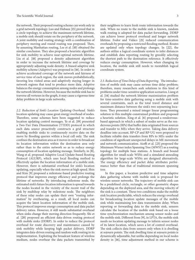
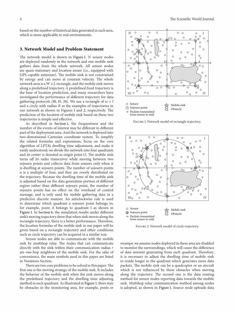
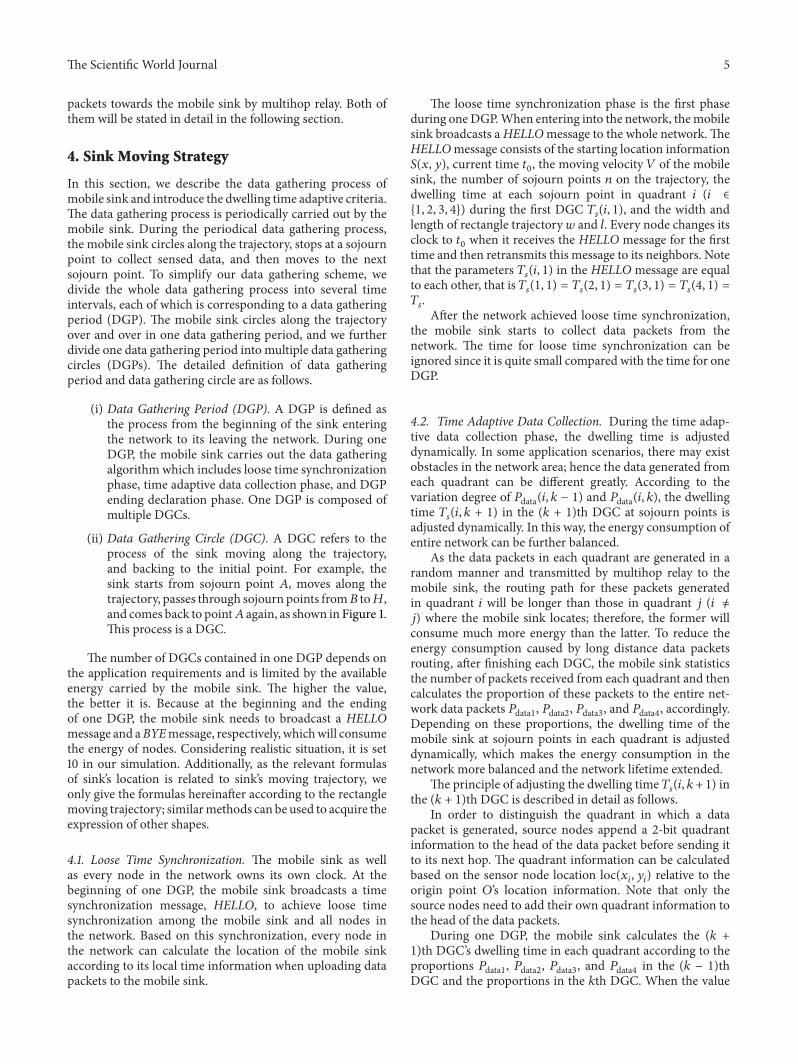
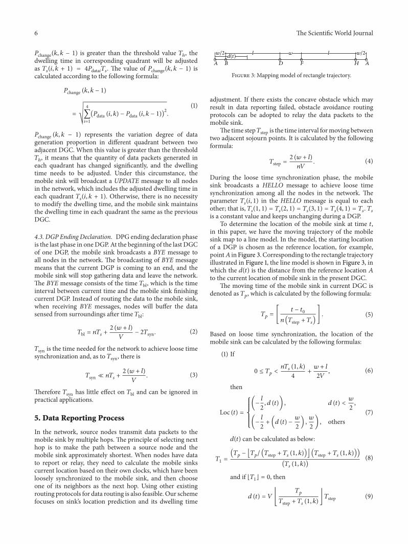
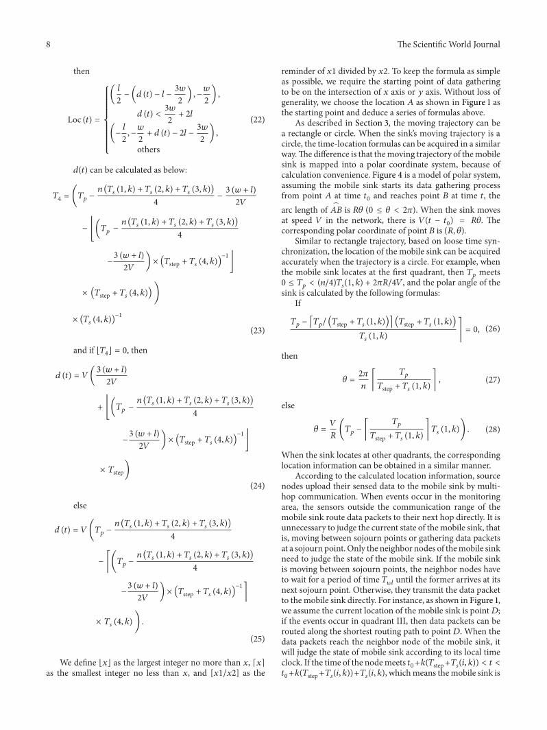
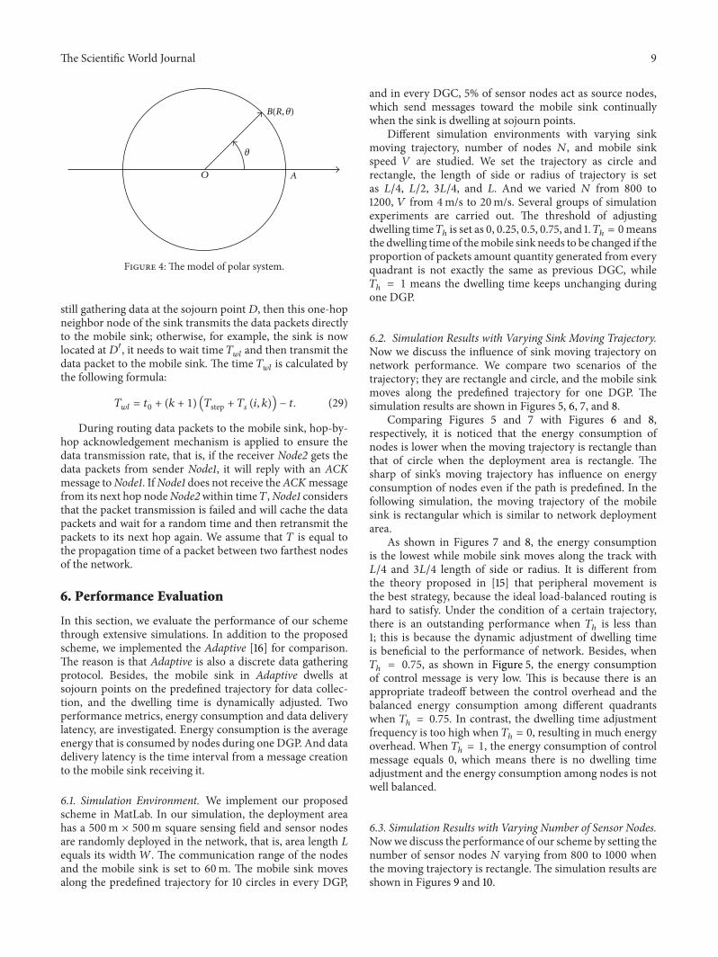
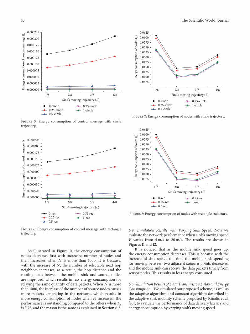
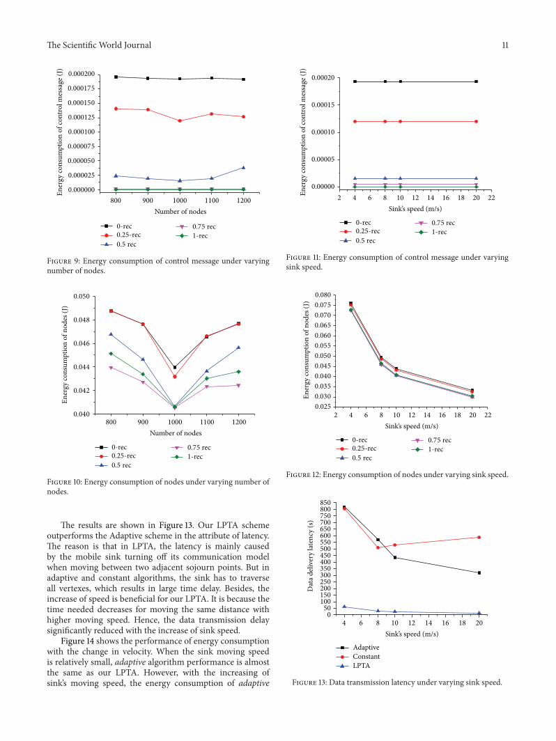
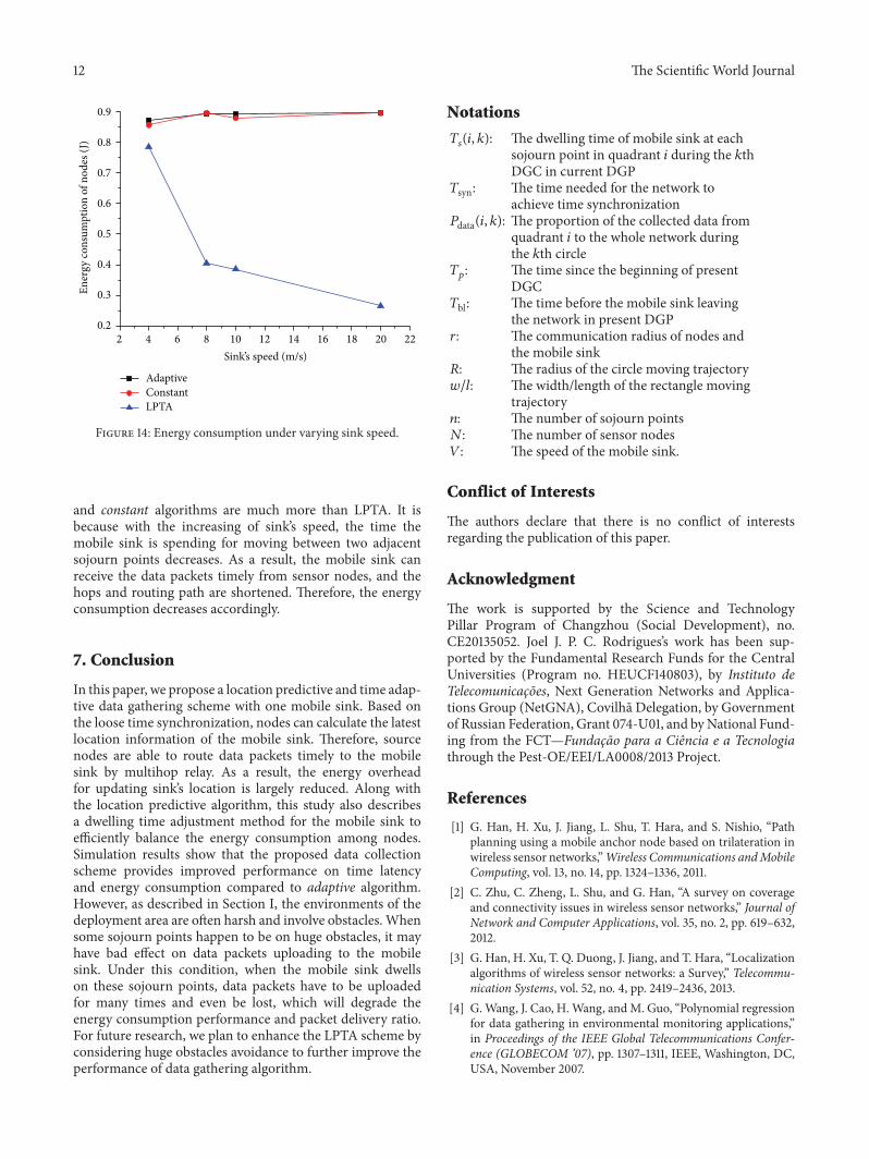


![NEWSLETTER The Valuers, Appraisers and Estate Agents … Sept 2018.pdf · 2018-10-03 · [2] Section 16(1) of the LPTA. [3] Section 2 of the LPTA. [4] Circular No 6 of Year 2017 on](https://static.fdocuments.us/doc/165x107/5e2a523f86813f268c5a564b/newsletter-the-valuers-appraisers-and-estate-agents-sept-2018pdf-2018-10-03.jpg)