Research Article Influence of the Constitutive Flow Law in...

Hindawi Publishing CorporationJournal of EngineeringVolume 2013, Article ID 231847, 8 pageshttp://dx.doi.org/10.1155/2013/231847

Research ArticleInfluence of the Constitutive Flow Law in FEM Simulation ofthe Radial Forging Process

Olivier Pantalé and Babacar Gueye

Universite de Toulouse, INP/ENIT, Laboratoire Genie de Production, 47 Avenue d’Azereix, 65016 Tarbes, France

Correspondence should be addressed to Olivier Pantale; [email protected]

Received 5 December 2012; Revised 23 April 2013; Accepted 23 April 2013

Academic Editor: Fabio Galbusera

Copyright © 2013 O. Pantale and B. Gueye. This is an open access article distributed under the Creative Commons AttributionLicense, which permits unrestricted use, distribution, and reproduction in any medium, provided the original work is properlycited.

Radial forging is a widely used forming process for manufacturing hollow products in transport industry. As the deformation of theworkpiece, during the process, is a consequence of a large number of high-speed strokes, the Johnson-Cook constitutive law (takinginto account the strain rate) seems to be well adapted for representing the material behavior even if the process is performed undercold conditions. But numerous contributions concerning radial forging analysis, in the literature, are based on a simple elastic-plastic formulation. As far as we know, this assumption has yet not been validated for the radial forging process. Because of theimportance of the flow law in the effectiveness of the model, our purpose in this paper is to analyze the influence of the use of anelastic-viscoplastic formulation instead of an elastic-plastic one for modeling the cold radial forging process. In this paper we haveselected two different laws for the simulations: the Johnson-Cook and the Ludwik ones, and we have compared the results in termsof forging force, product’s thickness, strains, stresses, and CPU time. For the presented study we use an AISI 4140 steel, and wedenote a fairly good agreement between the results obtained using both laws.

1. Introduction

Metal forming is a widely used tool in the industry to manu-facture a large range of parts in different sectors. Researchersand engineers have always resorted to some techniques inorder to improve their understanding of the process on theone hand, and on the other hand to properly control theprocess parameters and their influence on the producedworkpieces. The radial forging process is used to reduce thediameter of tubes and bars. The final shape of the workpieceis obtained thanks to a large number of strokes achieved byfour anvils radially arranged around the workpiece as shownin Figure 1. The preform is maintained in the proper positionand is pushed into the dies using a mandrel which grips itsecurely.Thepreform is subjected to a combination of an axialtranslation and a circumferential rotation.

For those studies, analyticalmethods have been originallydeveloped.Hosford andCaddell [1] in their contribution havedetailed many of such methods. One of these methods isthe work balance method is used to estimate the amount

of force required to achieve a metal forming operation. Inthe proposed approach, the global work is divided into threeparts: (a) an ideal work that would be required for onlythe shape change, (b) a friction work, and (c) an unwantedredundant work. The force required is estimated from thecomputation of the global energy involved in the formingoperation. Other approaches have also been used such as theone proposed by Ghaei et al. [2], based on the slab analysismethod, to compute the deformation versus the geometry ofthe die in a radial forging process. Choi et al. [3] employedthe upper-bound method to forecast the forging force. Theirresults were compared to experimental data, and a goodagreement was denoted for the proposed analytical model.Pitt-Francis et al. [4] have proposed a three-dimensionalformulation, also based on the upper bound method, toanalyze the forging process. In their contribution,Donald andChen [5] have developed an upper bound approach to analyzethe stability in soils and rocks. Even if those methods are veryuseful and simple to use, they are limited as soon as we needto get more detailed results concerning the material state. For

2 Journal of Engineering

Die sinusoidal motion

(I) Undeformed zone

I

(II) Conical zone

II

(III) Cylindrical extremity

III

Axial feedingDie land

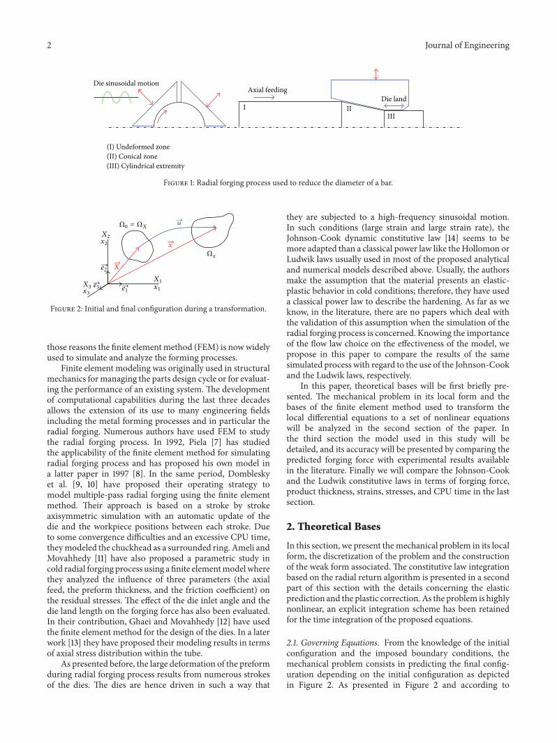
Figure 1: Radial forging process used to reduce the diameter of a bar.

𝑋2

𝑥2

𝑒2

𝑒3 𝑒1𝑥1

𝑋3

𝑋1

𝑥3

𝑥

𝑢

𝑋

Ω0 = Ω𝑋

Ω𝑥

→

→

→

→

→→

Figure 2: Initial and final configuration during a transformation.

those reasons the finite element method (FEM) is nowwidelyused to simulate and analyze the forming processes.

Finite element modeling was originally used in structuralmechanics for managing the parts design cycle or for evaluat-ing the performance of an existing system. The developmentof computational capabilities during the last three decadesallows the extension of its use to many engineering fieldsincluding the metal forming processes and in particular theradial forging. Numerous authors have used FEM to studythe radial forging process. In 1992, Piela [7] has studiedthe applicability of the finite element method for simulatingradial forging process and has proposed his own model ina latter paper in 1997 [8]. In the same period, Dombleskyet al. [9, 10] have proposed their operating strategy tomodel multiple-pass radial forging using the finite elementmethod. Their approach is based on a stroke by strokeaxisymmetric simulation with an automatic update of thedie and the workpiece positions between each stroke. Dueto some convergence difficulties and an excessive CPU time,theymodeled the chuckhead as a surrounded ring. Ameli andMovahhedy [11] have also proposed a parametric study incold radial forging process using a finite elementmodelwherethey analyzed the influence of three parameters (the axialfeed, the preform thickness, and the friction coefficient) onthe residual stresses. The effect of the die inlet angle and thedie land length on the forging force has also been evaluated.In their contribution, Ghaei and Movahhedy [12] have usedthe finite element method for the design of the dies. In a laterwork [13] they have proposed their modeling results in termsof axial stress distribution within the tube.

As presented before, the large deformation of the preformduring radial forging process results from numerous strokesof the dies. The dies are hence driven in such a way that

they are subjected to a high-frequency sinusoidal motion.In such conditions (large strain and large strain rate), theJohnson-Cook dynamic constitutive law [14] seems to bemore adapted than a classical power law like theHollomon orLudwik laws usually used in most of the proposed analyticaland numerical models described above. Usually, the authorsmake the assumption that the material presents an elastic-plastic behavior in cold conditions; therefore, they have useda classical power law to describe the hardening. As far as weknow, in the literature, there are no papers which deal withthe validation of this assumption when the simulation of theradial forging process is concerned. Knowing the importanceof the flow law choice on the effectiveness of the model, wepropose in this paper to compare the results of the samesimulated process with regard to the use of the Johnson-Cookand the Ludwik laws, respectively.

In this paper, theoretical bases will be first briefly pre-sented. The mechanical problem in its local form and thebases of the finite element method used to transform thelocal differential equations to a set of nonlinear equationswill be analyzed in the second section of the paper. Inthe third section the model used in this study will bedetailed, and its accuracy will be presented by comparing thepredicted forging force with experimental results availablein the literature. Finally we will compare the Johnson-Cookand the Ludwik constitutive laws in terms of forging force,product thickness, strains, stresses, and CPU time in the lastsection.

2. Theoretical Bases

In this section, we present themechanical problem in its localform, the discretization of the problem and the constructionof the weak form associated. The constitutive law integrationbased on the radial return algorithm is presented in a secondpart of this section with the details concerning the elasticprediction and the plastic correction. As the problem is highlynonlinear, an explicit integration scheme has been retainedfor the time integration of the proposed equations.

2.1. Governing Equations. From the knowledge of the initialconfiguration and the imposed boundary conditions, themechanical problem consists in predicting the final config-uration depending on the initial configuration as depictedin Figure 2. As presented in Figure 2 and according to

Journal of Engineering 3

Slave surface

Axial feeding

A: control point

Die motionA

Figure 3: Axisymmetric finite element model.

0

100

200

300

400

500

0 2 4 6 8 10 12 14 16 18Time (s)

Forc

e (kN

)

LudwikJohnson-Cook

(a)

1.6

D

D

C

C

B

B

A

A1.7

1.8

LudwikJohnson-Cook

0 10 20 30 40 50 60

Thic

knes

s (m

m)

Distance from point A (mm)

(b)

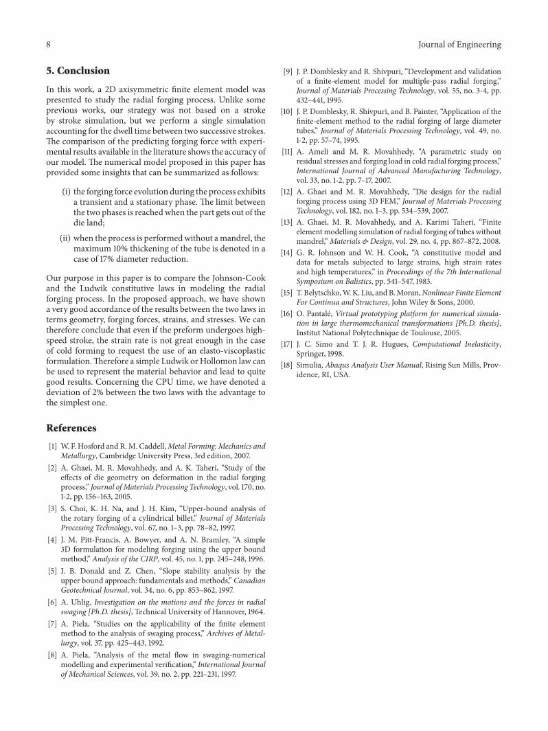
Figure 4: Numerically predicted forging force and geometry.

the continuum mechanics approach [15], we consider anarbitrary domainΩ with boundary Γ leading to the mechan-ical problem presented in (1) that must be solved at eachincrement. Consider,

∇ ⋅ 𝜎 + 𝜌�� = 𝜌 𝛾 in Ω

�� = ��𝑑 on Γ

𝑢

𝜎 ⋅ 𝑛 = 𝑡𝑑 on Γ

𝑑,

(1)

where ∇ is the divergence operator, 𝜎 is Cauchy stress tensor,𝜌�� is the body forces vector, 𝜌 is the mass density of thematerial, 𝛾 is the acceleration vector, �� is the displacementvector, 𝑛 is the surface normal vector, ⋅ is the contractionof inner indices operator,: is the double contractor of innerindices operator, and Γ𝑢 and Γ𝑑 are a partition of the domain’sboundary Γ, where displacements ��𝑑 and external loads 𝑡

𝑑 areimposed, respectively. In this state, the mechanical problemcannot be solved because of a lack of equations comparedto the unknown variables.Therefore the additional equationsgiven below are added to the previous system:

(i) the geometrical compatibility equation which is writ-ten in a general way as folows:

𝜀 =1

2[∇�� + (∇��)

𝑇

+ ∇�� ⋅ (∇��)𝑇

] , (2)

(ii) the constitutive equation used to represent the mate-rial behavior as a relation between different variables𝑓(𝜎, 𝜀, 𝜀, 𝑇) = 0, where 𝜀 is the strain tensor 𝜀 is thestrain rate tensor, and 𝑇 is the temperature.

2.2. Finite Element Discretization. The finite element methodis neither more or less than a mathematical way to resolvedifferential equations. It is an approximate method based onthe discretization of the problem’s equations and the domainin which a solution is looked for. In radial forming, themechanical problem is given by (1). Before resolution, thisequation is turned into a weak form by multiplying (1) withan admissible virtual displacement 𝛿�� and integrating in thehole domainΩ. So we obtain the following form on the wholedomain:

∫Ω

𝛿��𝜌��𝑑Ω + ∫Γ𝑑𝛿�� 𝑡𝑑𝑑Γ − ∫

Ω

𝛿𝜀 : 𝜎𝑑Ω

= ∫Ω

𝛿��𝜌��𝑑Ω.

(3)


𝑋

𝑌 𝑍

Peeq(Avg: 75%)

+2.898 − 01

+2.657𝑒

𝑒

𝑒

𝑒

− 01

+2.415𝑒 − 01

+2.174𝑒 − 01

+1.932 − 01

+1.691𝑒 − 01

+1.449𝑒 − 01

+1.208 − 01

+9.660 − 02

+7.245𝑒

𝑒

− 02

+4.830 − 02

+2.415𝑒

𝑒

𝑒

− 02

+0.000 + 00

Ludwik constitutive law

(a)

𝑋

𝑌 𝑍

Peeq(Avg: 75%)

+2.892𝑒 − 01

+2.651𝑒 − 01

+2.410𝑒 − 01

+2.169𝑒 − 01

+1.928𝑒 − 01

+1.687𝑒 − 01

+1.446𝑒 − 01

+1.205𝑒 − 01

+9.639𝑒 − 02

+7.229𝑒 − 02

+4.819𝑒 − 02

+2.410𝑒 − 02

+0.000𝑒 + 00

Johnson-Cook constitutive law

(b)

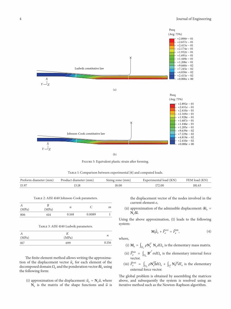
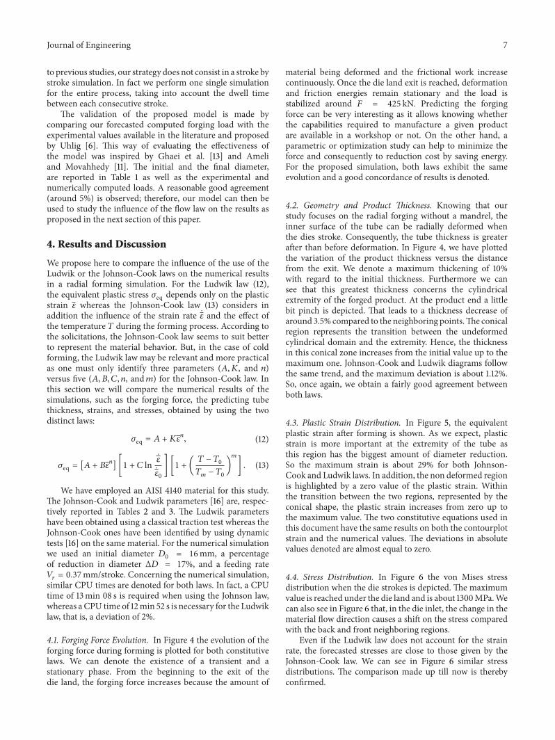
Figure 5: Equivalent plastic strain after forming.

Table 1: Comparison between experimental [6] and computed loads.

Preform diameter (mm) Product diameter (mm) Sizing zone (mm) Experimental load (KN) FEM load (KN)15.97 13.18 18.00 172.00 181.63

Table 2: AISI 4140 Johnson-Cook parameters.

𝐴

(MPa)𝐵

(MPa) 𝑛 𝐶 𝑚

806 614 0.168 0.0089 1

Table 3: AISI 4140 Ludwik parameters.

𝐴

(MPa)𝐾

(MPa) 𝑛

817 699 0.156

The finite element method allows writing the approxima-tion of the displacement vector ��𝑒 for each element of thedecomposed domainΩ𝑒 and the ponderation vector 𝛿��𝑒 usingthe following form:

(i) approximation of the displacement: ��𝑒 = N𝑒��, whereN𝑒 is the matrix of the shape functions and �� is

the displacement vector of the nodes involved in thecurrent element 𝑒,

(ii) approximation of the admissible displacement: 𝛿��𝑒 =N𝑒𝛿��.

Using the above approximation, (1) leads to the followingsystem:

M𝑒 ��𝑒 + ��ext𝑒

= ��int𝑒, (4)

where,

(i) M𝑒 = ∫Ω𝑒 𝜌N𝑇

𝑒N𝑒𝑑Ω𝑒 is the elementary mass matrix.

(ii) ��int𝑒

= ∫Ω𝑒

B𝑒𝑇

𝜎𝑑Ω𝑒 is the elementary internal forcevector.

(iii) ��ext𝑒

= ∫Ω𝑒𝜌N𝑇𝑒��𝑑Ω𝑒 + ∫

Γ𝑑𝑒

N𝑒 𝑡𝑑𝑑Γ𝑒 is the elementaryexternal force vector.

The global problem is obtained by assembling the matricesabove, and subsequently the system is resolved using aniterative method such as the Newton-Raphson algorithm.


𝑋

𝑌 𝑍

S, Mises(Avg: 75%)

+1.380 + 09

+1.266𝑒 + 09

+1.151𝑒 + 09

+1.036𝑒 + 09

+9.212 + 08

+8.064𝑒 + 08

+6.916𝑒 + 08

+5.768 + 08

+4.620 + 08

+3.472 + 08

+2.324𝑒

𝑒

𝑒

𝑒

𝑒

𝑒

𝑒

+ 08

+1.176𝑒 + 08

+2.812 + 06

Ludwik constitutive law

(a)

𝑋

𝑌 𝑍

S, Mises(Avg: 75%)

Johnson-Cook constitutive law

+1.295𝑒 + 09

+1.187𝑒

𝑒

𝑒

𝑒

𝑒

+ 09

+1.080 + 09

+9.720 + 08

+8.642 + 08

+7.565𝑒

𝑒

+ 08

+6.488 + 08

+5.411𝑒 + 08

+4.334𝑒 + 08

+3.257𝑒 + 08

+2.180 + 08

+1.103𝑒 + 08

+2.537𝑒 + 06

(b)

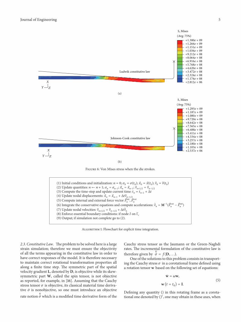
Figure 6: Von Mises stress when the die strokes.

(1) Initial conditions and initialization: 𝑛 = 0; 𝜎0= 𝜎(𝑡0); ��0= ��(𝑡0); V0= V(𝑡0)

(2) Update quantities: 𝑛 ← 𝑛 + 1; 𝜎𝑛 = 𝜎𝑛−1; ��𝑛 = ��𝑛−1; V𝑛+1/2 = V𝑛−1/2(3) Compute the time-step and update current time: 𝑡𝑛 = 𝑡𝑛−1 + Δ𝑡(4) Update nodal displacements: ��𝑛 = ��𝑛−1 + Δ𝑡V𝑛−1/2(5) Compute internal and external force vector ��int

𝑛, ��ext𝑛

(6) Integrate the conservative equations and compute accelerations: V𝑛 = M−1(��ext𝑛

− ��int𝑛)

(7) Update nodal velocities: V𝑛+1/2 = V𝑛−1/2 + Δ𝑡V𝑛

(8) Enforce essential boundary conditions: if node 𝐼 on ΓV(9) Output; if simulation not complete go to (2).

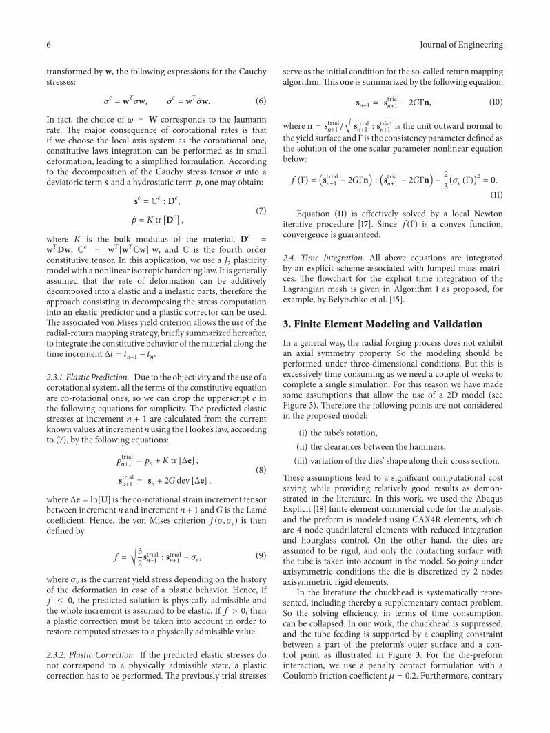
Algorithm 1: Flowchart for explicit time integration.

2.3. Constitutive Law. Theproblem to be solved here is a largestrain simulation; therefore we must ensure the objectivityof all the terms appearing in the constitutive law in order tohave correct responses of the model. It is therefore necessaryto maintain correct rotational transformation properties allalong a finite time step. The symmetric part of the spatialvelocity gradient L, denoted byD, is objective while its skew-symmetric part W, called the spin tensor, is not objectiveas reported, for example, in [16]. Assuming that the Cauchystress tensor 𝜎 is objective, its classical material time deriva-tive �� is nonobjective, so one must introduce an objectiverate notion

∇

𝜎 which is a modified time derivative form of the

Cauchy stress tensor as the Jaumann or the Green-Naghdirates. The incremental formulation of the constitutive law istherefore given by ∇𝜎 = 𝑓(D, . . .).

One of the solutions to this problem consists in transport-ing the Cauchy stress 𝜎 in a corotational frame defined usinga rotation tensor w based on the following set of equations:

w = 𝜔w,

w (𝑡 = 𝑡0) = I.(5)

Defining any quantity () in this rotating frame as a corota-tional one denoted by ()𝑐, one may obtain in these axes, when


transformed by w, the following expressions for the Cauchystresses:

𝜎𝑐= w𝑇𝜎w, ��

𝑐= w𝑇��w. (6)

In fact, the choice of 𝜔 = W corresponds to the Jaumannrate. The major consequence of corotational rates is thatif we choose the local axis system as the corotational one,constitutive laws integration can be performed as in smalldeformation, leading to a simplified formulation. Accordingto the decomposition of the Cauchy stress tensor 𝜎 into adeviatoric term s and a hydrostatic term 𝑝, one may obtain:

s𝑐 = C𝑐: D𝑐,

�� = 𝐾 tr [D𝑐] ,(7)

where 𝐾 is the bulk modulus of the material, D𝑐 =

w𝑇Dw, C𝑐 = w𝑇[w𝑇Cw] w, and C is the fourth orderconstitutive tensor. In this application, we use a 𝐽2 plasticitymodel with a nonlinear isotropic hardening law. It is generallyassumed that the rate of deformation can be additivelydecomposed into a elastic and a inelastic parts; therefore theapproach consisting in decomposing the stress computationinto an elastic predictor and a plastic corrector can be used.The associated von Mises yield criterion allows the use of theradial-returnmapping strategy, briefly summarized hereafter,to integrate the constitutive behavior of thematerial along thetime increment Δ𝑡 = 𝑡𝑛+1 − 𝑡𝑛.

2.3.1. Elastic Prediction. Due to the objectivity and the use of acorotational system, all the terms of the constitutive equationare co-rotational ones, so we can drop the upperscript 𝑐 inthe following equations for simplicity. The predicted elasticstresses at increment 𝑛 + 1 are calculated from the currentknown values at increment 𝑛 using theHooke’s law, accordingto (7), by the following equations:

𝑝trial𝑛+1

= 𝑝𝑛 + 𝐾 tr [Δe] ,

strial𝑛+1

= s𝑛 + 2𝐺 dev [Δe] ,(8)

whereΔe = ln[U] is the co-rotational strain increment tensorbetween increment 𝑛 and increment 𝑛 + 1 and 𝐺 is the Lamecoefficient. Hence, the von Mises criterion 𝑓(𝜎, 𝜎V) is thendefined by

𝑓 = √3

2strial𝑛+1

: strial𝑛+1

− 𝜎V,(9)

where 𝜎V is the current yield stress depending on the historyof the deformation in case of a plastic behavior. Hence, if𝑓 ≤ 0, the predicted solution is physically admissible andthe whole increment is assumed to be elastic. If 𝑓 > 0, thena plastic correction must be taken into account in order torestore computed stresses to a physically admissible value.

2.3.2. Plastic Correction. If the predicted elastic stresses donot correspond to a physically admissible state, a plasticcorrection has to be performed. The previously trial stresses

serve as the initial condition for the so-called returnmappingalgorithm.This one is summarized by the following equation:

s𝑛+1 = strial𝑛+1

− 2𝐺Γn, (10)

where n = strial𝑛+1

/√ strial𝑛+1

: strial𝑛+1

is the unit outward normal tothe yield surface and Γ is the consistency parameter defined asthe solution of the one scalar parameter nonlinear equationbelow:

𝑓 (Γ) = (strial𝑛+1

− 2𝐺Γn) : (strial𝑛+1

− 2𝐺Γn) − 2

3(𝜎V (Γ))

2= 0.

(11)

Equation (11) is effectively solved by a local Newtoniterative procedure [17]. Since 𝑓(Γ) is a convex function,convergence is guaranteed.

2.4. Time Integration. All above equations are integratedby an explicit scheme associated with lumped mass matri-ces. The flowchart for the explicit time integration of theLagrangian mesh is given in Algorithm 1 as proposed, forexample, by Belytschko et al. [15].

3. Finite Element Modeling and Validation

In a general way, the radial forging process does not exhibitan axial symmetry property. So the modeling should beperformed under three-dimensional conditions. But this isexcessively time consuming as we need a couple of weeks tocomplete a single simulation. For this reason we have madesome assumptions that allow the use of a 2D model (seeFigure 3). Therefore the following points are not consideredin the proposed model:

(i) the tube’s rotation,(ii) the clearances between the hammers,(iii) variation of the dies’ shape along their cross section.

These assumptions lead to a significant computational costsaving while providing relatively good results as demon-strated in the literature. In this work, we used the AbaqusExplicit [18] finite element commercial code for the analysis,and the preform is modeled using CAX4R elements, whichare 4 node quadrilateral elements with reduced integrationand hourglass control. On the other hand, the dies areassumed to be rigid, and only the contacting surface withthe tube is taken into account in the model. So going underaxisymmetric conditions the die is discretized by 2 nodesaxisymmetric rigid elements.

In the literature the chuckhead is systematically repre-sented, including thereby a supplementary contact problem.So the solving efficiency, in terms of time consumption,can be collapsed. In our work, the chuckhead is suppressed,and the tube feeding is supported by a coupling constraintbetween a part of the preform’s outer surface and a con-trol point as illustrated in Figure 3. For the die-preforminteraction, we use a penalty contact formulation with aCoulomb friction coefficient 𝜇 = 0.2. Furthermore, contrary


to previous studies, our strategy does not consist in a stroke bystroke simulation. In fact we perform one single simulationfor the entire process, taking into account the dwell timebetween each consecutive stroke.

The validation of the proposed model is made bycomparing our forecasted computed forging load with theexperimental values available in the literature and proposedby Uhlig [6]. This way of evaluating the effectiveness ofthe model was inspired by Ghaei et al. [13] and Ameliand Movahhedy [11]. The initial and the final diameter,are reported in Table 1 as well as the experimental andnumerically computed loads. A reasonable good agreement(around 5%) is observed; therefore, our model can then beused to study the influence of the flow law on the results asproposed in the next section of this paper.

4. Results and Discussion

We propose here to compare the influence of the use of theLudwik or the Johnson-Cook laws on the numerical resultsin a radial forming simulation. For the Ludwik law (12),the equivalent plastic stress 𝜎eq depends only on the plasticstrain 𝜀 whereas the Johnson-Cook law (13) considers inaddition the influence of the strain rate 𝜀 and the effect ofthe temperature 𝑇 during the forming process. According tothe solicitations, the Johnson-Cook law seems to suit betterto represent the material behavior. But, in the case of coldforming, the Ludwik law may be relevant and more practicalas one must only identify three parameters (𝐴,𝐾, and 𝑛)versus five (𝐴, 𝐵, 𝐶, 𝑛, and𝑚) for the Johnson-Cook law. Inthis section we will compare the numerical results of thesimulations, such as the forging force, the predicting tubethickness, strains, and stresses, obtained by using the twodistinct laws:

𝜎eq = 𝐴 + 𝐾𝜀𝑛, (12)

𝜎eq = [𝐴 + 𝐵𝜀𝑛] [1 + 𝐶 ln

𝜀

𝜀0

] [1 + (𝑇 − 𝑇0

𝑇𝑚 − 𝑇0

)

𝑚

] . (13)

We have employed an AISI 4140 material for this study.The Johnson-Cook and Ludwik parameters [16] are, respec-tively reported in Tables 2 and 3. The Ludwik parametershave been obtained using a classical traction test whereas theJohnson-Cook ones have been identified by using dynamictests [16] on the same material. For the numerical simulationwe used an initial diameter 𝐷0 = 16mm, a percentageof reduction in diameter Δ𝐷 = 17%, and a feeding rate𝑉𝑟 = 0.37mm/stroke. Concerning the numerical simulation,similar CPU times are denoted for both laws. In fact, a CPUtime of 13min 08 s is required when using the Johnson law,whereas a CPU time of 12min 52 s is necessary for the Ludwiklaw, that is, a deviation of 2%.

4.1. Forging Force Evolution. In Figure 4 the evolution of theforging force during forming is plotted for both constitutivelaws. We can denote the existence of a transient and astationary phase. From the beginning to the exit of thedie land, the forging force increases because the amount of

material being deformed and the frictional work increasecontinuously. Once the die land exit is reached, deformationand friction energies remain stationary and the load isstabilized around 𝐹 = 425 kN. Predicting the forgingforce can be very interesting as it allows knowing whetherthe capabilities required to manufacture a given productare available in a workshop or not. On the other hand, aparametric or optimization study can help to minimize theforce and consequently to reduction cost by saving energy.For the proposed simulation, both laws exhibit the sameevolution and a good concordance of results is denoted.

4.2. Geometry and Product Thickness. Knowing that ourstudy focuses on the radial forging without a mandrel, theinner surface of the tube can be radially deformed whenthe dies stroke. Consequently, the tube thickness is greaterafter than before deformation. In Figure 4, we have plottedthe variation of the product thickness versus the distancefrom the exit. We denote a maximum thickening of 10%with regard to the initial thickness. Furthermore we cansee that this greatest thickness concerns the cylindricalextremity of the forged product. At the product end a littlebit pinch is depicted. That leads to a thickness decrease ofaround 3.5% compared to the neighboring points.The conicalregion represents the transition between the undeformedcylindrical domain and the extremity. Hence, the thicknessin this conical zone increases from the initial value up to themaximum one. Johnson-Cook and Ludwik diagrams followthe same trend, and the maximum deviation is about 1.12%.So, once again, we obtain a fairly good agreement betweenboth laws.

4.3. Plastic Strain Distribution. In Figure 5, the equivalentplastic strain after forming is shown. As we expect, plasticstrain is more important at the extremity of the tube asthis region has the biggest amount of diameter reduction.So the maximum strain is about 29% for both Johnson-Cook and Ludwik laws. In addition, the non deformed regionis highlighted by a zero value of the plastic strain. Withinthe transition between the two regions, represented by theconical shape, the plastic strain increases from zero up tothe maximum value. The two constitutive equations used inthis document have the same results on both the contourplotstrain and the numerical values. The deviations in absolutevalues denoted are almost equal to zero.

4.4. Stress Distribution. In Figure 6 the von Mises stressdistribution when the die strokes is depicted. The maximumvalue is reached under the die land and is about 1300MPa.Wecan also see in Figure 6 that, in the die inlet, the change in thematerial flow direction causes a shift on the stress comparedwith the back and front neighboring regions.

Even if the Ludwik law does not account for the strainrate, the forecasted stresses are close to those given by theJohnson-Cook law. We can see in Figure 6 similar stressdistributions. The comparison made up till now is therebyconfirmed.


5. Conclusion

In this work, a 2D axisymmetric finite element model waspresented to study the radial forging process. Unlike someprevious works, our strategy was not based on a strokeby stroke simulation, but we perform a single simulationaccounting for the dwell time between two successive strokes.The comparison of the predicting forging force with experi-mental results available in the literature shows the accuracy ofour model. The numerical model proposed in this paper hasprovided some insights that can be summarized as follows:

(i) the forging force evolution during the process exhibitsa transient and a stationary phase. The limit betweenthe two phases is reachedwhen the part gets out of thedie land;

(ii) when the process is performedwithout amandrel, themaximum 10% thickening of the tube is denoted in acase of 17% diameter reduction.

Our purpose in this paper is to compare the Johnson-Cookand the Ludwik constitutive laws in modeling the radialforging process. In the proposed approach, we have showna very good accordance of the results between the two laws interms geometry, forging forces, strains, and stresses. We cantherefore conclude that even if the preform undergoes high-speed stroke, the strain rate is not great enough in the caseof cold forming to request the use of an elasto-viscoplasticformulation.Therefore a simple Ludwik orHollomon law canbe used to represent the material behavior and lead to quitegood results. Concerning the CPU time, we have denoted adeviation of 2% between the two laws with the advantage tothe simplest one.

References

[1] W. F. Hosford and R.M. Caddell,Metal Forming: Mechanics andMetallurgy, Cambridge University Press, 3rd edition, 2007.

[2] A. Ghaei, M. R. Movahhedy, and A. K. Taheri, “Study of theeffects of die geometry on deformation in the radial forgingprocess,” Journal ofMaterials Processing Technology, vol. 170, no.1-2, pp. 156–163, 2005.

[3] S. Choi, K. H. Na, and J. H. Kim, “Upper-bound analysis ofthe rotary forging of a cylindrical billet,” Journal of MaterialsProcessing Technology, vol. 67, no. 1–3, pp. 78–82, 1997.

[4] J. M. Pitt-Francis, A. Bowyer, and A. N. Bramley, “A simple3D formulation for modeling forging using the upper boundmethod,” Analysis of the CIRP, vol. 45, no. 1, pp. 245–248, 1996.

[5] I. B. Donald and Z. Chen, “Slope stability analysis by theupper bound approach: fundamentals and methods,” CanadianGeotechnical Journal, vol. 34, no. 6, pp. 853–862, 1997.

[6] A. Uhlig, Investigation on the motions and the forces in radialswaging [Ph.D. thesis], Technical University of Hannover, 1964.

[7] A. Piela, “Studies on the applicability of the finite elementmethod to the analysis of swaging process,” Archives of Metal-lurgy, vol. 37, pp. 425–443, 1992.

[8] A. Piela, “Analysis of the metal flow in swaging-numericalmodelling and experimental verification,” International Journalof Mechanical Sciences, vol. 39, no. 2, pp. 221–231, 1997.

[9] J. P. Domblesky and R. Shivpuri, “Development and validationof a finite-element model for multiple-pass radial forging,”Journal of Materials Processing Technology, vol. 55, no. 3-4, pp.432–441, 1995.

[10] J. P. Domblesky, R. Shivpuri, and B. Painter, “Application of thefinite-element method to the radial forging of large diametertubes,” Journal of Materials Processing Technology, vol. 49, no.1-2, pp. 57–74, 1995.

[11] A. Ameli and M. R. Movahhedy, “A parametric study onresidual stresses and forging load in cold radial forging process,”International Journal of Advanced Manufacturing Technology,vol. 33, no. 1-2, pp. 7–17, 2007.

[12] A. Ghaei and M. R. Movahhedy, “Die design for the radialforging process using 3D FEM,” Journal of Materials ProcessingTechnology, vol. 182, no. 1–3, pp. 534–539, 2007.

[13] A. Ghaei, M. R. Movahhedy, and A. Karimi Taheri, “Finiteelementmodelling simulation of radial forging of tubes withoutmandrel,”Materials & Design, vol. 29, no. 4, pp. 867–872, 2008.

[14] G. R. Johnson and W. H. Cook, “A constitutive model anddata for metals subjected to large strains, high strain ratesand high temperatures,” in Proceedings of the 7th InternationalSymposium on Balistics, pp. 541–547, 1983.

[15] T. Belytschko,W.K. Liu, andB.Moran,Nonlinear Finite ElementFor Continua and Structures, John Wiley & Sons, 2000.

[16] O. Pantale, Virtual prototyping platform for numerical simula-tion in large thermomechanical transformations [Ph.D. thesis],Institut National Polytechnique de Toulouse, 2005.

[17] J. C. Simo and T. J. R. Hugues, Computational Inelasticity,Springer, 1998.

[18] Simulia, Abaqus Analysis User Manual, Rising Sun Mills, Prov-idence, RI, USA.

International Journal of

AerospaceEngineeringHindawi Publishing Corporationhttp://www.hindawi.com Volume 2014

RoboticsJournal of

Hindawi Publishing Corporationhttp://www.hindawi.com Volume 2014


Active and Passive Electronic Components

Control Scienceand Engineering

Journal of



RotatingMachinery


Hindawi Publishing Corporation http://www.hindawi.com

Journal ofEngineeringVolume 2014

Submit your manuscripts athttp://www.hindawi.com

VLSI Design



Shock and Vibration


Civil EngineeringAdvances in

Acoustics and VibrationAdvances in



Electrical and Computer Engineering

Journal of

Advances inOptoElectronics

Hindawi Publishing Corporation http://www.hindawi.com

Volume 2014

The Scientific World JournalHindawi Publishing Corporation http://www.hindawi.com Volume 2014

SensorsJournal of


Modelling & Simulation in EngineeringHindawi Publishing Corporation http://www.hindawi.com Volume 2014


Chemical EngineeringInternational Journal of Antennas and

Propagation




Navigation and Observation



DistributedSensor Networks


Research Article Influence of the Constitutive Flow Law in...

Documents

Transcript of Research Article Influence of the Constitutive Flow Law in...