Research Article Hopf Bifurcation Characteristics of...
21
Research Article Hopf Bifurcation Characteristics of Dual-Front Axle Self-Excited Shimmy System for Heavy Truck considering Dry Friction Daogao Wei, 1 Ke Xu, 1 Yibin Jiang, 1 Changhe Chen, 1 Wenjing Zhao, 1 and Fugeng Zhou 2 1 School of Mechanical and Automotive Engineering, Hefei University of Technology, Hefei 230009, China 2 China Anhui Jianghuai Automobile Co., Ltd., Hefei 230022, China Correspondence should be addressed to Daogao Wei; [email protected] Received 19 April 2015; Accepted 13 August 2015 Academic Editor: Marcello Vanali Copyright © 2015 Daogao Wei et al. is is an open access article distributed under the Creative Commons Attribution License, which permits unrestricted use, distribution, and reproduction in any medium, provided the original work is properly cited. Multiaxle steering is widely used in commercial vehicles. However, the mechanism of the self-excited shimmy produced by the multiaxle steering system is not clear until now. is study takes a dual-front axle heavy truck as sample vehicle and considers the influences of mid-shiſt transmission and dry friction to develop a 9 DOF dynamics model based on Lagrange’s equation. Based on the Hopf bifurcation theorem and center manifold theory, the study shows that dual-front axle shimmy is a self-excited vibration produced from Hopf bifurcation. e numerical method is adopted to determine how the size of dry friction torque influences the Hopf bifurcation characteristics of the system and to analyze the speed range of limit cycles and numerical characteristics of the shimmy system. e consistency of results of the qualitative and numerical methods shows that qualitative methods can predict the bifurcation characteristics of shimmy systems. e influences of the main system parameters on the shimmy system are also discussed. Improving the steering transition rod stiffness and dry friction torque and selecting a smaller pneumatic trail and caster angle can reduce the self-excited shimmy, reduce tire wear, and improve the driving stability of vehicles. 1. Introduction In recent years, with the rapid development of the trans- portation industry, high-speed and multiaxle heavy trucks with dual-front axles have become widely used for their load capacity, high performance-price ratio, adaptability, and high horsepower. e dual-front axle steering system is a relatively advanced steering system given its low cost, simple handling, steering safety and stability under heavy load, and the less harm it causes on the road surface during driving. However, the shimmy problem in its dual-front axle steering system leads to abnormal tire wear (especially the tire on the second axle), off-tracking, and shaking of the steering wheel [1–3]. Research on the shimmy of single-axle vehicles can be traced back to 80 years ago and can be classified into forced shimmy and self-excited shimmy, which is a Hopf bifurcation phenomenon. Extensive research has been conducted on this field and can be used to solve the shimmy problems in engineering [4–7]. Given the growth in the demand for multiaxle heavy trucks, current research on the dual-axle steering system shimmy has demonstrated its significance. Considering its sophisticated mechanism, the shimmy of a dual-axle steering system differs from that of a single- axle steering system. erefore, many scholars have studied the problem extensively. Watanabe et al. [1] studied the effect of the number and position of driving wheels on the steering performance of dual-axle steering vehicles. Gu et al. [8] demonstrated the content and method in the design of heavy trucks with a multiaxle steering system, analyzed the main problems in this research field in China, and proposed a design method for a steering system based on integrated and optimized matching platform for a chassis system. Hou et al. [9] established the kinematics model and a mathematical optimization model for the multiaxle steering system of 10 × 8 heavy-duty vehicle and designed a new weight function considering the probability of steering angle. e parameters of multiaxle steering system were optimized. e result showed that the result with weight function had better effect than other conditions. Wang et al. [10] applied a robust design theory with design parameters and noise factors following a normal distribution in a dual-front axle steering system. He combined reliability optimization Hindawi Publishing Corporation Shock and Vibration Volume 2015, Article ID 839801, 20 pages http://dx.doi.org/10.1155/2015/839801
Transcript of Research Article Hopf Bifurcation Characteristics of...

Research ArticleHopf Bifurcation Characteristics of Dual-Front Axle Self-ExcitedShimmy System for Heavy Truck considering Dry Friction
Daogao Wei1 Ke Xu1 Yibin Jiang1 Changhe Chen1 Wenjing Zhao1 and Fugeng Zhou2
1School of Mechanical and Automotive Engineering Hefei University of Technology Hefei 230009 China2China Anhui Jianghuai Automobile Co Ltd Hefei 230022 China
Correspondence should be addressed to Daogao Wei weidaogaohfuteducn
Received 19 April 2015 Accepted 13 August 2015
Academic Editor Marcello Vanali
Copyright copy 2015 Daogao Wei et al This is an open access article distributed under the Creative Commons Attribution Licensewhich permits unrestricted use distribution and reproduction in any medium provided the original work is properly cited
Multiaxle steering is widely used in commercial vehicles However the mechanism of the self-excited shimmy produced by themultiaxle steering system is not clear until now This study takes a dual-front axle heavy truck as sample vehicle and considers theinfluences of mid-shift transmission and dry friction to develop a 9 DOF dynamics model based on Lagrangersquos equation Based onthe Hopf bifurcation theorem and center manifold theory the study shows that dual-front axle shimmy is a self-excited vibrationproduced from Hopf bifurcationThe numerical method is adopted to determine how the size of dry friction torque influences theHopf bifurcation characteristics of the system and to analyze the speed range of limit cycles and numerical characteristics of theshimmy system The consistency of results of the qualitative and numerical methods shows that qualitative methods can predictthe bifurcation characteristics of shimmy systems The influences of the main system parameters on the shimmy system are alsodiscussed Improving the steering transition rod stiffness and dry friction torque and selecting a smaller pneumatic trail and casterangle can reduce the self-excited shimmy reduce tire wear and improve the driving stability of vehicles
1 Introduction
In recent years with the rapid development of the trans-portation industry high-speed and multiaxle heavy truckswith dual-front axles have become widely used for their loadcapacity high performance-price ratio adaptability and highhorsepowerThe dual-front axle steering system is a relativelyadvanced steering system given its low cost simple handlingsteering safety and stability under heavy load and the lessharm it causes on the road surface during driving Howeverthe shimmy problem in its dual-front axle steering systemleads to abnormal tire wear (especially the tire on the secondaxle) off-tracking and shaking of the steering wheel [1ndash3]
Research on the shimmy of single-axle vehicles can betraced back to 80 years ago and can be classified into forcedshimmy and self-excited shimmy which is a Hopf bifurcationphenomenon Extensive research has been conducted onthis field and can be used to solve the shimmy problemsin engineering [4ndash7] Given the growth in the demand formultiaxle heavy trucks current research on the dual-axlesteering system shimmy has demonstrated its significance
Considering its sophisticated mechanism the shimmy ofa dual-axle steering system differs from that of a single-axle steering system Therefore many scholars have studiedthe problem extensively Watanabe et al [1] studied theeffect of the number and position of driving wheels on thesteering performance of dual-axle steering vehicles Gu et al[8] demonstrated the content and method in the designof heavy trucks with a multiaxle steering system analyzedthe main problems in this research field in China andproposed a design method for a steering system based onintegrated and optimized matching platform for a chassissystem Hou et al [9] established the kinematics model and amathematical optimization model for the multiaxle steeringsystem of 10 times 8 heavy-duty vehicle and designed a newweight function considering the probability of steering angleThe parameters of multiaxle steering system were optimizedThe result showed that the result with weight functionhad better effect than other conditions Wang et al [10]applied a robust design theory with design parameters andnoise factors following a normal distribution in a dual-frontaxle steering system He combined reliability optimization
Hindawi Publishing CorporationShock and VibrationVolume 2015 Article ID 839801 20 pageshttpdxdoiorg1011552015839801
2 Shock and Vibration
with robust design and built a mathematical model forthe robust reliability optimization of dual-front axles withclearances Xu et al [11] developed a steering wheel shimmymodel for a four-axis steering crane without considering thenonlinear factors and their impact on the four-axis steeringcrane shimmy Nisonger and Wormley [12] compared thetransverse dynamic characteristics of single- and dual-frontaxle steering systems using a nonlinear model with threedegrees of freedom Wu and Lin [13] found that the double-front axle can improve a carrsquos yaw stability Williams [14]extended the dual-axle model for vehicles to a multiaxlemodel and analyzed its steering ability and handling stabilityBy analyzing a linear dual-front axle yaw dynamics modelDemic [15] analyzed the influence of structural parameterson the front wheel shimmy of a heavy vehicle and foundthat the vibration of suspension can cause front wheelshimmy Cole and Cebon [16] developed a vibration modelfor the pneumatic suspension of a heavy truck to reducethe vibration in and damage to the road surface caused bytrucks through suspension parameter optimization Chen[17] concluded that two reasonsmdashinternal and externalmdashaccount for abnormal tire wear proposed improvementmeasures based on his practical experience and pointed outdirections for future research Liao [18] and Li et al [19]explored the application of multirigid body theory in thedynamic simulation of a dual-front axle steering system andproposed the condition underwhich tires bear heavy load in adual-front axle vehicle They also built a spatial model for thedual-front axle based onADAMSand conducted a simulationanalysis Using TruckSim a dynamics analysis software forvehicles Li [20] studied how to determine and describe theseven characteristic parameters of a heavy truck steeringsystem namely axle and suspension transmission tire bodybrake system and aerodynamics and laid down a solidfoundation for the study ofmultiaxle steering technology andthe improvement of its handling stability
Most of the aforementioned studies focus on the con-structional parameter analysis and simulation of dual-frontaxle steering system however there is little research onsteering system shimmy especially there is little research onthe mechanism of Hopf bifurcation produce self-shimmyBut it is not yet clear about Hopf bifurcation characteristicof dual-front axle self-shimmy for heavy truck Thereforethe research in this area is very important In this studywe took a JAC heavy truck as an example and establishednine degrees of freedom equations for the dual-front axlesteering systembased onLagrangersquos equationWedeterminedthe existence and the value of Hopf bifurcation with the useof the Hurwitz criterion [21] and Hopf bifurcation theoremTo obtain the manifold for the system in two-dimensionalspace we reduced the dimension of the differential equationsof state using center manifold theory and found the Hopfparadigm in the polar coordinates with the use of normativetheory so that the Hopf bifurcation characteristics of theshimmy system of the dual-front axles can be fully analyzedBased on the above analysis we then propose a methodof controlling such shimmy As such this study establishesthe theoretical foundation for research on the mechanismof the dual-front axle self-excited shimmy and provides
V
1205791
1205792
1205793
1205794
Figure 1 Schematic of dual-front axle steering system
Steeringgear
Firsttransition
rod1205751
r1
g1r2
1205752 g2
r3
1205753 g3
Anteriorlongitudinal
rod
Intermediaterocker
Secondtransition
rod
Firstrocker
Posteriorlongitudinal rod
Secondrocker
sim
Figure 2 Schematic of intermediate steering transmission mecha-nism
a reference on the design improvement of steering systemsThe contribution of this study is the finding that the self-excited shimmy phenomenon of the dual-front axle of aheavy truck is generated by Hopf bifurcation
2 Dynamics Model for a Dual-Front AxleShimmy System
21 Mechanical Model The schematic of the structure ofthe widely used dual-front axle steering system is shown inFigure 1 the diagram of the steering intermediate transmis-sion is shown in Figure 2 To facilitate the development ofthe mathematical model of the dual-front axle self-excitedshimmy system the mechanics model of the dual-front axleself-excited shimmy system is developed based on Figure 2with the dual-front axle steering system of a JAC heavy truckas prototype the schematics of which are shown in Figure 3Figure 3 illustrates the double-front axle steering principlethe steering force exerted by the driver is passed throughthe steering operating mechanism which is composed of thesteering shaft transmission shaft and steering joints towardsthe steering gear (2)The torque is then transmitted to the firstrocker (3) after its torque increases and its speed decreasesThe first rocker (3) then drives the steering knuckle arm (5)
of the first steering bridge through the anterior longitudinalrod (4) to turn the left wheel to rotate around the kingpinwhich is installed in the first steering bridge At the sametime the right wheel driven by the torque which passes
Shock and Vibration 3
1
2
34
5
67
1314 8
15
910
11
12
kc
kz1cz1
kt1ct1 kh1
ch1
1205931
cz2kz2
kh2
ch2
kt2
ct2
1205932
(1) Steering wheel(2) Steering gear(3) First rocker(4) Anterior longitudinal rod(5) Steering knuckle arm(6) First transition rod(7) Intermediate rocker(8) Tie rod
(9) Second transition rod(10) Second rocker(11) Steering power cylinder(12) Posterior longitudinal rod(13) Tire(14) Left trapezoid arm(15) Right trapezoid arm
Figure 3 Dual-front axle shimmy system mechanics model
through the left trapezoid arm (14) to the tie rod (8) to theright trapezoid arm (15) rotates The second bridge steeringis consistent with the first bridge steering and the steeringforce is passed through the first transition rod (6) to theintermediate rocker (7) to the second transition rod (9) to thesecond rocker (10) to the posterior longitudinal rod (12) andto the second bridge
In the mechanical model the elasticity of the rod isconsidered it is equivalent to a spring-damper unit In linewith the law of the right-hand coordinate system the centerof the mass of the vehicle is deemed as the coordinate originthe vehicle forward direction is for 119909-axis the vehicle leftdirection is for 119910-axis and perpendicular to the ground updirection is for 119911-axis Figure 3 shows that the system hasnearly 20 rotating hinges To facilitate the dynamic analysisand mathematical modeling and to highlight the effect ofmultisport hinges dry friction and other parameters ofthe self-excited shimmy system as shown in Figure 3 thefollowing assumptions are made to establish a dynamicsmodel for the dual-front axle steering shimmy system (1)The steering wheel is immobile (2) The impact of the forceof air is ignored (3) The various parts associated with thevibration and their couplings are simplified according to themoments of inertia springs and dampers (4) The anglebetween the steering trapezoid plane and 119883119884 plane and theangle between the steering linkage and the 119883119885 plane areignored (5)Thedirection and speed of the vehicle is constant(6) Longitudinal and lateral slips do not occur in the vehicle(7)The dry friction in the kinematic pairs is equivalent to thekingpin of the first or second bridge
22 The Equation for the Motion of the Shimmy SystemAccording to the dynamics model in Figure 3 we established
the equations for the motion of the dual-front axle steeringshimmy system of heavy vehicles The shimmy system hasnine degrees of freedom 120579
1is the swing angle at which the
left wheel of the first bridge rotates around the kingpin 1205792is
the swing angle at which the right wheel of the first bridgerotates around the kingpin 120593
1is the lateral swing angle of the
first bridge 1205793is the swing angle at which the left wheel of
the second bridge rotates around the kingpin 1205794is the swing
angle at which the right wheel of the second bridge rotatesaround the kingpin 120593
2is the lateral swing angle of the second
bridge 1205751is the swing angle of the first rocking arm 120575
2is the
swing angle of the intermediate steering arm 1205753is the swing
angle of the second rocking armIn this study the mathematical model of the shimmy
system of the sample vehicle is established using Lagrangersquosequations which can be expressed as
119889
119889119905
(
120597119879
120597119896
) minus
120597119879
120597119902119896
+
120597119880
120597119902119896
+
120597119863
120597119896
= 119876119896
(119896 = 1 2 3 9)
(1)
where 119902119896represents nine degrees of freedom of the system
119879 represents the systemrsquos kinetic energy 119880 represents thesystemrsquos potential energy119863 represents the systemrsquos dissipatedenergy and 119876
119896represents the nine generalized forces to
which the system is subjectedAccording to Figure 3 kinetic energy potential energy
dissipated energy and the nine generalized forces of the dual-front axle steering shimmy system are obtained as follows
4 Shock and Vibration
The kinetic energy of the shimmy system is
119879 =
1
2
1198681(1205791
2
+1205792
2
) +
1
2
11986911
2+
1
2
1198682(1205793
2
+1205794
2
) +
1
2
11986922
2
+
1
2
1198681198881
1205751
2
+
1
2
1198681198882
1205752
2
+
1
2
1198681198883
1205753
2
(2)
where 119868119894(119894 = 1 2) is the moment of inertia of the wheel
around the kingpin in 119894th bridge 119868119888119894(119894 = 1 3) is the moment
of inertia of 119894th rocker 1198681198882
is the moment of inertia of theintermediate rocker and 119869
119894(119894 = 1 2) is the moment of inertia
of 119894th bridge around its side off-axisThe potential energy of the shimmy system is
119880 =
1
2
119896ℎ1(1205791minus 1205792)2
+
1
2
1198961198991205931
2+
1
2
119896ℎ2(1205793minus 1205794)2
+
1
2
1198961198991205932
2+
1
2
1198961199051205751
2+
1
2
1198961199051(11989211205751minus 11990321205752)2
+
1
2
1198961199052(11989221205752minus 11989231205753)2
+
1
2
1198961199111(11990311205751+ 11988611205792)2
+
1
2
1198961199112(11990331205753+ 11988621205794)2
(3)
where 119896ℎ119894(119894 = 1 2) is the stiffness of the tie rod converted
into the stiffness around the kingpin 119896119899is the equivalent
angle stiffness of the suspension converted into the side swingcenter 119896
119905is the inverse stiffness of the first rocking arm
to the steering wheel 119896119905119894(119894 = 1 2) is the stiffness of 119894th
transition rod 119896119911119894(119894 = 1 2) is the stiffness of the front and rear
longitudinal rods 1199031is the effective length of the first arm 119903
2is
the effective length of themiddle arm 1199033is the effective length
of the second arm11989211198922 and119892
3are the distances between the
pivot point of the rocker and the transition lever and the fixedend of the rocker arm and 119886
119894(119894 = 1 2) is the distance between
the hinge point of 119894th bridge knuckle arm and vertical rod andkingpin
The dissipated energy of the shimmy system is
119863 =
1
2
1198881198971(1205791+
1205792) +
1
2
119888ℎ1(1205791minus
1205792)
2
+
1
2
1198881198991
2
+
1
2
119888ℎ2(1205793minus
1205794)
2
+
1
2
1198881198972(1205793+
1205794) +
1
2
1198881198992
2
+
1
2
1198881199051205751
2
+
1
2
1198881199051(11989211205751minus 11990321205752)
2
+
1
2
1198881199052(11989221205752minus 11989231205753)
2
+
1
2
1198881199111(11990311205751+ 11988611205792)
2
+
1
2
1198881199112(11990331205753+ 11988621205794)
2
+11987222
1205794+11987221
1205793+11987212
1205792
+11987211
1205791
(4)
where 119888119897119894(119894 = 1 2) is the equivalent damping of 119894th wheel
around the kingpin 119888ℎ119894(119894 = 1 2) is the damping of the tie
rod converted into the damping around the kingpin 119888119899is the
equivalent damping of the suspension converted into the sideswing center 119888
119905is the inverse damping of the first rocking
arm to the steering wheel 119888119905119894(119894 = 1 2) is the damping of
119894th transition rod 119888119911119894(119894 = 1 2) is the damping of the front
and rear longitudinal rods 11987211
is the equivalent frictiontorque of the first bridge at the right wheel kingpin119872
12is the
equivalent friction torque of the first bridge at the left wheelkingpin 119872
21is the equivalent friction torque of the second
bridge at the right wheel kingpin and 11987222
is the equivalentfriction torque of the second bridge at the left wheel kingpin
The nine generalized forces of the shimmy system are asfollows for details about the procedure for calculation of thegeneralized forces see appendix
1198761= minus1198941198961
V119877
1+ 1198651(119877120574 + 119890)
minus (120574120588ℎ1119877 +
119896119888
2
11986111198971(minus119891 + 120574))120593
1
1198762= minus1198941198961
V119877
1+ 1198652(119877120574 + 119890)
minus (120574120588ℎ1119877 +
119896119888
2
11986111198971(minus119891 + 120574))120593
1
1198763= minus2120588119877ℎ
11205931+ 1198941198961
V119877
(1205791+
1205792) minus (119865
1+ 1198652) 119877
1198764= minus1198941198962
V119877
2+ 1198653(119877120574 + 119890)
minus (120574120588ℎ2119877 +
119896119888
2
11986121198972(minus119891 + 120574))120593
2
1198765= minus1198941198962
V119877
2+ 1198654(119877120574 + 119890)
minus (120574120588ℎ2119877 +
119896119888
2
11986121198972(minus119891 + 120574))120593
2
1198766= minus2120588119877ℎ
21205932+ 1198941198962
V119877
(1205793+
1205794) minus (119865
3+ 1198654) 119877
1198767= 0
1198768= 0
1198769= 0
(5)
where 119894119896119894(119894 = 1 2) is the moment of inertia of the wheel
around its own axis of rotation in 119894th bridge V is the vehiclespeed 119877 is the rolling radius of the tire 119865
1is the first bridge
right wheel subjected to lateral force 1198652is the first bridge left
wheel subjected to lateral force 1198653is the second bridge right
wheel subjected to lateral force 1198654is the second bridge left
wheel subjected to lateral force 120574 is the kingpin caster angle ofthe wheel 119890 is the pneumatic trail 120588 is the tire lateral stiffnessℎ119894is the height of 119894th suspension roll center (119894 = 1 2) 119896
119888
is the tire vertical stiffness 119861119894(119894 = 1 2) is the tread in 119894th
bridge 119897119894(119894 = 1 2) is the distance between the point of the
kingpin extension linewith the ground intersection and planeof symmetry of thewheel119891 is the friction coefficient betweenthe tire and the ground and 120590 is the tire relaxation length
According to (2) to (5) the kinetic equations for thesystem are derived from Lagrangersquos equations as given by (1)
Shock and Vibration 5
Equations for the motion of the right wheel of the firstbridge around the kingpin are as follows
11986811205791+ 1198881198971
1205791+ 119896ℎ1(1205791minus 1205792) + 119888ℎ1(1205791minus
1205792) +
1198941198961V
119877
1
+ (120588119877ℎ1120574 +
1
2
11989611988811989711198611(120574 minus 119891)) 120593
1minus 1198651(119877120574 + 119890)
+11987211= 0
(6)
Equations for the motion of the left wheel of the first bridgearound the kingpin are as follows
11986811205792+ 1198881198971
1205792+ 119896ℎ1(1205792minus 1205791) + 119888ℎ1(1205792minus
1205791)
+ 11989611991111198861(11990311205751+ 11988611205792) + 11988811991111198861(11990311205751+ 11988611205792)
+
1198941198961V
119877
1+ (120588119877ℎ
1120574 +
1
2
11989611988811989711198611(120574 minus 119891)) 120593
1
minus 1198652(119877120574 + 119890) +119872
12= 0
(7)
Lateral swing equations for the motion of the first bridge areas follows
11986911+ 11988811989911+ (
1
2
1198961198881198611
2+ 119896119899+ 2120588119877ℎ
1)1205931
minus
1198941198961V
119877
(1205791+
1205792) + (119865
1+ 1198652) ℎ1= 0
(8)
Equations for the motion of the right wheel of the secondbridge around the kingpin are as follows
11986821205793+ 1198881198972
1205793+ 119896ℎ2(1205793minus 1205794) + 119888ℎ2(1205793minus
1205794) +
1198941198962V
119877
2
+ (120588119877ℎ2120574 +
1
2
11989611988811989721198612(120574 minus 119891)) 120593
2minus 1198653(119877120574 + 119890)
+11987221= 0
(9)
Equations for themotion of the leftwheel of the secondbridgearound the kingpin are as follows
11986821205794+ 1198881198972
1205792+ 119896ℎ2(1205794minus 1205793) + 119888ℎ2(1205794minus
1205793)
+ 11989611991121198862(11990331205753+ 11988621205794) + 11988811991121198862(11990331205753+ 11988621205794)
+
1198941198962V
119877
2+ (120588119877ℎ
2120574 +
1
2
11989611988811989721198612(120574 minus 119891)) 120593
2
minus 1198654(119877120574 + 119890) +119872
22= 0
(10)
Lateral swing equations for the motion of the second bridgeare as follows
11986922+ 11988811989922+ (
1
2
1198961198881198612
2+ 119896119899+ 2120588119877ℎ
2)1205932
minus
1198941198962V
119877
(1205793+
1205794) + (119865
3+ 1198654) ℎ2= 0
(11)
Magic formulaCubic formula
minus6 minus4 minus2minus8 2 4 60 8
Side-slip angle 120572 (∘)
minus4000
minus3000
minus2000
minus1000
0
1000
2000
3000
4000
Tire
forc
eF(N
)
Figure 4 Curve of relationship between 119865119894and 120572
119894
Swing equations for the motion of the first rocking arm are asfollows
1198681198881
1205751+ 1198881199051205751+ 1198961199051205751+ 11988811990511198921(11989211205751minus 11990321205752)
+ 11989611990511198921(11989211205751minus 11990321205752) + 11988811991111199031(11990311205751+ 11988611205792)
+ 11989611991111199031(11990311205751+ 11988611205792) = 0
(12)
Swing equations for the motion of the intermediate steeringarm are as follows
1198681198882
1205752+ 11988811990511199032(11990321205752minus 11989211205751) + 11989611990511199032(11990321205752minus 11989211205751)
+ 11988811990521198922(11989221205752minus 11989231205753) + 11989611990521198922(11989221205752minus 11989231205753)
= 0
(13)
Swing equations for themotion of the second rocking arm areas follows
1198681198883
1205753+ 11988811990521198923(11989231205753minus 11989221205752) + 11989611990521198923(11989231205753minus 11989221205752)
+ 11988811991121199033(11990331205753+ 11988621205794) + 11989611991121199033(11990331205753+ 11988621205794) = 0
(14)
23 Tire Model Selection Several nonlinear tire models arecommonly used in the simulation of vehicle dynamics suchas Pacejkarsquos magic formula cubemodel Guo Konghuirsquos semi-empirical tire theoretical model and Gimrsquos tire models [22ndash25] Equations (15) and (16) are the mathematical expressionsof the cube and magic formula models respectively Thecornering force curves of these two tire models are shownin Figure 4 which shows that two cornering force curveshave the same trend and that the cube model is similar tothe magic formula Moreover the cube model is simple itdoes not require a considerable amount of experimental datacan precisely reveal the performance characteristic trends of
6 Shock and Vibration
Table 1 Parameters of tire model
1198621119891
1198623119891
1198861
1198862
1198863
1198864
1198865
1198866
1198867
1198868
32740 481770 minus221 1011 1078 182 0208 0 minus0354 0707
the tire force and does not contain trigonometric functionsthereby facilitating qualitative analysis As such we choosethe cube model as the tire model in this study The cubemodel is the third-order truncation of themagic formula [23]The coefficients (119861
119894 119863119894 and 119864
119894) of magic formula take into
account the impact of the vertical load119865119885119894 So the cubemodel
cube considers the vertical force 119865119885119894
119865119894= minus (119862
1119891120572119894minus 1198623119891120572119894
3) (119894 = 1 2 3 4) (15)
119865119894= 119863119894sin (119862
119894
times arctan (119861119894119886119894minus 119864119894(119861119894119886119894minus arctan (119861
119894119886119894))))
(16)
In this model
119861119894=
1198863sdot sin (119886
4sdot (arctan (119886
5sdot 119865119885119894)))
119862119894sdot 119863119894
119862119894= 13
119863119894= 1198861sdot 119865119885119894
2+ 1198862sdot 119865119885119894
119864119894= 1198866sdot 119865119885119894
2+ 1198867sdot 119865119885119894+ 1198868
(119894 = 1 2 3 4)
(17)
where 1198621119891
and 1198623119891
are the fitting coefficients of the tire120572119894(119894 = 1 2 3 4 denote the first bridge right wheel the first
bridge left wheel the second bridge right wheel and thesecond bridge left wheel resp) is the side-slip angle of thetire 119861
119894 119862119894 119863119894 and 119864
119894denote the stiffness shape crest and
curvature factors respectively 1198861 1198862 1198863 1198864 1198865 1198866 1198867 and 119886
8
are obtained by test fitting 119865119885119894
is the vertical forces on thetires For details see appendix about 119865
119885119894 1198621119891 and 119862
3119891 The
required values [26 27] are shown in Table 1The relationship curve between the tire force 119865
119894and the
side-slip angle 120572119894is shown in Figure 4
The following are the tire rolling nonholonomic con-straint equations [28] namely the relationship between slipangle and the shimmy angle
119894+
V120590
120572119894+
V120590
120579119894minus
119890119894
120590
120579119894 119894 = 1 2 3 4 (18)
24 Dry Friction Model Selection In this study the dryfrictions in the suspension and steeringmechanism ball kine-matic pairs and steering gear kinematic pairs are consideredSuspension and steering systems are complex self-excitedshimmy systems thus we made the kinematic pairs dryfriction of the suspension and the steering system exceptfor the dry friction in the kingpin equivalent to that ofthe kingpin because the dry friction in the kingpin is themain component of sports vice dry friction We studied onlythe effect of the value of dry friction torque on the Hopf
bifurcation of the shimmy system and therefore we changeonly the dry friction torque 119872 when making numericalcalculations
We selected the Coulomb model as the ideal frictionmodel in this study It has a constant value and is alwaysin the opposite direction of the relative motion This kindof friction always impedes movement and is always in theopposite direction of the movement speed Its mathematicalexpression is
119872119894119895= 119872 sgn (
120579119894119895) (119894 119895 = 1 2)
|119872| =
120583119904119873119903 (
120579119894119895= 0)
120583119873119903 (120579119894119895
= 0)
(119894 119895 = 1 2)
(19)
where 120583 is the coefficient of sliding friction 120583119904is the
coefficient of static friction 119873 denotes a positive pressureand 119903 is the main pin radius
The parameter values of the sample vehicle are shown inTable 2
3 Hopf Bifurcation Qualitative Analysis ofthe Shimmy System
31 Existence Analysis of Hopf Bifurcation The existenceanalysis and stability assessment of Hopf bifurcation in anonlinear system are the most fundamental and importantassessments in studying the dynamics of a nonlinear systemHurwitz criterion is applied to investigate the existence ofHopf bifurcation in the dual-front axle shimmy system Thecenter manifold approach is applied to reduce and simplifythe nonlinear system and obtain a two-dimensional systemThe Hopf bifurcation paradigm is then applied to investigatethe stability of the bifurcation of limit cycles
Make 1199091= 1205791 1199092=
1205791 1199093= 1205792 1199094=
1205792 1199095= 1205931 1199096= 1
1199097= 1205793 1199098=
1205793 1199099= 1205794 11990910
=1205794 11990911
= 1205932 11990912
= 2
11990913
= 1205751 11990914
=1205751 11990915
= 1205752 11990916
=1205752 11990917
= 1205753 11990918
=1205753
11990919
= 1205721 11990920
= 1205722 11990921
= 1205723 and 119909
22= 1205724 Assume 119883 =
(1199091 1199092 1199093 1199094 1199095 1199096 1199097 1199098 1199099 11990910 11990911 11990912 11990913 11990914 11990915 11990916
11990917 11990918 11990919 11990920 11990921 11990922) according to the theory of
nonlinear dynamics the equilibrium point1198830is obtained by
solving the system static equations Equations (6) to (14) canbe expressed as the following static equations
= 119860119883 + 119865 (119883) 119883 isin 11987722 (20)
where 119860 is the Jacobian matrix in the equilibrium pointvicinity of the system and 119865(119883) contains quadratic and cubicnonlinear terms
According to Hurwitz criterion the equilibrium point ofthe system is stable when V = V
1or when V = V
2 whereas
the equilibrium point of the system is unstable when V1le
V le V2and when the critical speeds are V
1= 156 kmh and
V2= 408 kmh The eigenvalues of the Jacobian matrix 119860 are
shown in Table 3According to Table 3 the Jacobian matrix119860 of the system
has a pair of purely imaginary eigenvalues when V = V1and
V = V2 and the other eigenvalues have negative real parts
Shock and Vibration 7
Table 2 Sample car parameter values
Parameter Value1198681 1198682kgsdotm2sdotradminus1 168
1198691 1198692kgsdotm2sdotradminus1 2108
1198681198881kgsdotm2sdotradminus1 038
1198681198882kgsdotm2sdotradminus1 022
1198681198883kgsdotm2sdotradminus1 028
1198941198961 1198941198962kgsdotm2sdotradminus1 142
119896ℎ1 119896ℎ2Nsdotradminus1 37790
119888ℎ1 119888ℎ2Nsdotmsdotssdotradminus1 25
1198881198971 1198881198972Nsdotmsdotssdotradminus1 42
119896119899Nsdotradminus1 31360
119888119899Nsdotmsdotssdotradminus1 1027
1205741 1205742∘ 25
1198971 1198972m 007
1199031m 034
1199033m 047
1198922m 026
1198861m 021
1198961199111 1198961199112Nsdotradminus1 36000
1198881199111 1198881199112Nsdotmsdotssdotradminus1 30
1198961199051 1198961199052Nsdotmminus1 37200
1198881199051 1198881199052Nsdots 15
119896119888Nsdotradminus1 1060000
119891 0015119896119905Nsdotradminus1 31000
119888119905Nsdotmsdotssdotradminus1 10
120588Nsdotradminus1 765000119877m 0511198901 1198902m 007
ℎ1 ℎ2m 045
1198611 1198612m 206
1199032m 042
1198921m 017
1198923m 022
1198862m 021
Using theHopf bifurcation theorem as basis we can concludethat the critical speeds V
1= 156 kmh and V
2= 408 kmh are
the bifurcation points of the systems and a two-dimensionalcenter manifold exists When V
1le V le V
2 positive real part
eigenvalues exist and the original shimmy system has self-excited vibrations and produces limit cycles When V lt V
1
or V gt V2 all the eigenvalues of 119860 have negative real parts
and the original shimmy system is stable asymptotically andeventually becomes balanced
32 Stability Analysis of Limit Cycles The center manifoldapproach is applied to determine the stability of the originalsystem in low-dimensional systems and to reduce the originalsystem Assuming 120583
119896= VminusV
119896(119896 = 1 2) 120583
119896is an increment in
the speed bifurcation parameter at the bifurcation point andhas a minimum value Using the nonsingular transformation119883 = 119875119884 where 119884 has the same dimensions as 119883 119875
Table 3 Eigenvalues of Jacobian matrix 119860 corresponding to thecritical speed
V1corresponding eigenvalues V
2corresponding eigenvalues
1205821
0 + 1211119894 1205821
0 + 1456119894
1205822
0 minus 1211119894 1205822
0 minus 1456119894
1205823
minus16544 + 78083119894 1205823
minus16544 + 78083119894
1205824
minus16544 minus 78083119894 1205824
minus16544 minus 78083119894
1205825
minus7140 + 54908119894 1205825
minus7140 + 54908119894
1205826
minus7140 minus 54908119894 1205826
minus7140 minus 54908119894
1205827
minus437 + 6315119894 1205827
minus425 + 6316119894
1205828
minus437 minus 6315119894 1205828
minus425 minus 6316119894
1205829
minus434 + 6178119894 1205829
minus422 + 6179119894
12058210
minus434 minus 6178119894 12058210
minus422 minus 6179119894
12058211
minus218 + 2688119894 12058211
minus162 + 2773119894
12058212
minus218 minus 2688119894 12058212
minus162 minus 2773119894
12058213
minus224 + 2681119894 12058213
minus179 + 2746119894
12058214
minus224 minus 2681119894 12058214
minus179 minus 2746119894
12058215
minus122 + 1621119894 12058215
minus098 + 1765119894
12058216
minus122 minus 1621119894 12058216
minus098 minus 1765119894
12058217
minus24378 + 91155119894 12058217
minus24378 + 91155119894
12058218
minus24378 minus 91155119894 12058218
minus24378 minus 91155119894
12058219
minus892 12058219
minus1514
12058220
minus664 12058220
minus1358
12058221
minus355 12058221
minus909
12058222
minus354 12058222
minus910
is composed of the real and imaginary parts of all theeigenvectors andΛ = 119875
minus1119860119875 is 22times22 diagonal matrix (20)
is converted into
= Λ119884 + 119875minus1119892 (119884 120583
119896) (21)
Using center manifold theory to reduce dimension thecenter manifold 119882
119888 of the expansion system represented by(21) is tangent to the plane of (119910
1 1199102 120583119896) at the singular point
(1198830 V0) assuming the center manifold
119910119894= ℎ119894(1199101 1199102 120583119896)
= ℎ11989411199101
2+ ℎ11989421205831198961199101+ ℎ11989431205831198961199102+ ℎ11989441199102
2
119894 = 3 4 21 22
(22)
119894=
120597ℎ119894(1199101 1199102 120583119896)
1205971199101
1+
120597ℎ119894(1199101 1199102 120583119896)
1205971199102
2
+
120597ℎ119894(1199101 1199102 120583119896)
120597120583119896
120583119896
(23)
Equation (22) is substituted into (21) and is then com-bined with (23) after which the coefficients of the same itemon both sides of the equation are compared using the softwareMaple In solving the linear equations the coefficients ofℎ119894(1199101 1199102 V) (119894 = 3 4 21 22) can be obtained and brought
into the previous two equations of (21) After simplifying
8 Shock and Vibration
the equation reduction equations can be obtained when V1=
156 kmh or V2= 408 kmh at the center manifold
When V = V1= 156 kmh the reduction equation is
1= 121 times 10119910
2+ 0762119910
21205831minus 0396119910
11205831minus 0169
times 10minus311991021205831
2minus 0156 times 10
minus41199102
3minus 0118
times 10minus311991011205831
2minus 0556 times 10
minus311991011199102
2minus 066
times 10minus21199101
21199102minus 0261 times 10
minus11199101
3+ 0426
times 10minus41199101
211991021205831+ 0464 times 10
minus41199101
31205831
2= minus121 times 10119910
1minus 0148119910
11205831+ 0853119910
21205831+ 0998
times 10minus411991011205831
2+ 0113 times 10
minus11199101
3+ 0429
times 10minus411991021205831
2+ 0286 times 10
minus21199101
21199102+ 0242
times 10minus311991011199102
2minus 0201 times 10
minus41199101
31205831minus 0187
times 10minus41199101
211991021205831
(24)
When V = V2= 408 kmh the reduction equation is
1= 146 times 10119910
2minus 0414 times 10
minus21199101+ 0522119910
21205832
minus 055011991011205832minus 0784 times 10
minus21199102
3+ 0118
times 10minus411991011205832
2minus 0487 times 10
minus11199102
21199101
minus 010111991021199101
2minus 0697 times 10
minus11199101
3minus 0259
times 10minus411991021199101
21205832minus 0231 times 10
minus41199101
31205832
2= minus146 times 10119910
1minus 0414 times 10
minus21199102+ 0275
times 10minus111991011205832+ 0261119910
21205832+ 0381
times 10minus411991011205832
2+ 0391 times 10
minus11199101
3minus 0531
times 10minus411991021205832
2+ 0565 times 10
minus111991021199101
2+ 0273
times 10minus11199102
21199101+ 0439 times 10
minus21199102
3+ 0103
times 10minus41199101
31205832+ 0116 times 10
minus411991021199101
21205832
(25)
According to the literature [29] the Hopf bifurcationparadigm under the polar coordinates of (24) to (25) can beobtained using Maple procedures
119903 = dur + 1198861199033+ hot
120579 = 120596 + 119887119903
2+ hot
(26)
where hot represents infinitesimals of higher orderAccording to (24)sim(28) we can obtain the following
F
120583sN120583N
r
minus120583Nminus120583sN
Figure 5 Shimmy system friction with the change of velocity curve
For V = V1= 156 kmh
119903 = (minus0751 times 10minus41205831+ 0229) 120583
1119903 + (minus0193
times 10minus6
1205831
2+ 0236 times 10
minus41205831minus 0106 times 10
minus1) 1199033
+ hot
(27)
For V = V2= 408 kmh
119903 = (minus0413 times 10minus4
1205832minus 0145) 120583
2119903 + (minus0495
times 10minus6
1205832
2minus 0133 times 10
minus4
1205832minus 0476 times 10
minus1
) 1199033
+ hot
(28)
According to (27) and (28) we can obtain the bifurcationdiagram at equilibrium point119883
0of each critical velocity The
diagram is shown in Figure 6According to Figure 6 Hopf bifurcations are supercritical
at the critical speeds V1and V
2 When V lt V
1= 156 kmh
(ie 1205831lt 0) shimmy does not occur in the system that is
the system is stable and equilibrium point1198830is a stable focus
When V1lt V lt V
2(ie 120583
1gt 0 and 120583
2lt 0) shimmy occurs in
the system equilibrium point 1198830is an unstable focus and a
stable limit cycle appears The phenomenon of the mutationof a stable focus into a stable limit cycle is called the limit cyclehard to produce or stable hard lossWhen V gt V
2= 408 kmh
(ie 1205832gt 0) the equilibrium point turns into a stable focus
again the limit cycle disappears the shimmy phenomenondisappears and the system tends to be stableThus dual-frontaxle shimmy is a typical self-excited vibration
4 Calculation and Analysis of the HopfBifurcation in the Shimmy System
41 Numerical Calculation and Analysis Using the motionequations of the sample vehicle shimmy system and theRunge-Kutta method for the numerical calculation ofshimmy systems the bifurcation diagrams in Figure 7 showthat the left wheel swing angles of the first and second bridgesvary with speed
Shock and Vibration 9
minus0015 minus001 minus0005 0 0005 001 0015 002minus002
Bifurcation parameter 1205831
minus08
minus06
minus04
minus02
0
02
04
06
08H
opf b
ifurc
atio
n br
anch
r
(a) Bifurcation diagram at V1
minus04
minus03
minus02
minus01
0
01
02
03
04
minus0015 minus001 minus0005 0 0005 001 0015 002minus002
Bifurcation parameter 1205832
Hop
f bifu
rcat
ion
bran
chr
(b) Bifurcation diagram at V2
Figure 6 Bifurcation diagram of1198830at two critical speeds
20 40 60 80 100 120 1400Velocity V (kmh)
0
05
1
15
2
25
3
35
4
Firs
t brid
ge le
ft w
heel
swin
g an
gle1205792
(∘)
(a) First bridge left wheel
20 40 60 80 100 120 1400Velocity V (kmh)
0
2
4
6
8
10
12Se
cond
brid
ge le
ft w
heel
swin
g an
gle1205794
(∘)
(b) Second bridge left wheel
20 40 60 80 100 120 1400Velocity V (kmh)
0
002
004
006
008
01
012
014
016
018
02
Firs
t brid
ge si
de sw
ing
angl
e1205931
(∘)
(c) The first bridge side pendulum
20 40 60 80 100 120 1400Velocity V (kmh)
0
01
02
03
04
Seco
nd b
ridge
side
swin
g an
gle1205932
(∘)
05
06
(d) The second bridge side pendulum
Figure 7 First and second bridge Hopf bifurcation with change of speed
According to Figure 7 when V lt 156 kmh and V gt
408 kmh the vibration of a dual-front axle system graduallystabilizes whereas when 156 kmh lt V lt 408 kmh periodicoscillations occur in the dual-front axle steering systemresulting in the limit cycle These results are consistent with
the qualitative calculation results in Section 31 which in turnshow that the theoretical qualitative methods are consistentwith the numerical methods
To better analyze the state changes in a dual-front axlesystem within the shimmy speed range we provide a swing
10 Shock and Vibration
First bridgeSecond bridge
minus10minus15 minus5 10 1550
Left wheel swing angles 1205792 1205794 (∘)
minus150
minus100
minus50
0
50
100
150
Ang
ular
vel
ociti
es120579998400 2120579
998400 4(∘
s)
(a) V = 20 kmh
First bridgeSecond bridge
minus10minus15 minus5 10 1550
Left wheel swing angles 1205792 1205794 (∘)
minus150
minus100
minus50
0
50
100
150
Ang
ular
vel
ociti
es120579998400 2120579
998400 4(∘
s)
(b) V = 25 kmh
First bridgeSecond bridge
minus150
minus100
minus50
0
50
100
150
minus5 0 5 10minus10
Left wheel swing angles 1205792 1205794 (∘)
Ang
ular
vel
ociti
es120579998400 2120579
998400 4(∘
s)
(c) V = 30 kmh
Figure 8 Phase diagram of the two front wheels at different speed
angle phase diagram of the left wheel of the first and secondbridges of heavy-duty vehicles under different speeds asshown in Figure 8
The conclusions on the shimmy characteristics and lawspertaining to the left wheel of the first and second bridgesunder different speeds as shown in Figures 8(a)ndash8(c) aredrawn The results are summarized in Table 4
(1) From Figures 8(a) to 8(c) in the bifurcation speedrange the shimmy of the steering wheel is the limitcycle vibration with a larger amplitude When thespeed increases the self-excited oscillation ampli-tude of the swing angle increases initially and thendecreases and the amplitude of the swing angle accel-eration has the same trend The maximum amplitude
Table 4 Shimmy characteristic at different speed
Vkmsdothminus1 20 25 301205792∘ 373 381 328
1205794∘ 1055 1092 947
Δ120579∘ 682 711 6191205792radsdotsminus1 083 086 0761205794radsdotsminus1 231 246 221
Δ120579radsdotsminus1 148 159 144
of the swing angle of the left wheel of the first bridge is381∘ and the maximum amplitude of the swing angleacceleration is 086 radsThemaximum amplitude ofthe swing angle of the left wheel of the second bridge
Shock and Vibration 11
First bridgeSecond bridge
minus5
0
5A
ngul
ar v
eloc
ities
120593998400 1120593
998400 2(∘
s)
0 05minus05
Side swing angles 1205931 1205932 (∘)
(a) V = 20 kmh
First bridgeSecond bridge
minus6
minus4
minus2
0
2
4
6
0 05minus05
Ang
ular
vel
ociti
es120593998400 1120593
998400 2(∘
s)
Side swing angles 1205931 1205932 (∘)
(b) V = 25 kmh
First bridgeSecond bridge
minus6
minus4
minus2
0
2
4
6
0 05minus05
Ang
ular
vel
ociti
es120593998400 1120593
998400 2(∘
s)
Side swing angles 1205931 1205932 (∘)
(c) V = 30 kmh
Figure 9 Phase diagram of the two bridges side pendulum at different speed
is 1092∘ and the maximum amplitude of the swingangle acceleration is 246 rads This phenomenonleads the vehicle to huntingmovement andmakes thedriver feel the tension and fatigue
(2) According to Figures 8(a)ndash8(c) and Table 4 the vari-ations in the left wheel swing angle differences andangular acceleration differences of the first and thesecond bridges are consistent with the variationsin the swing angles and angular accelerations Themaximum difference between the left wheel swingangles of the two bridges is 711∘ whereas the min-imum difference is 619∘ The maximum differenceof the angular acceleration is 159 rads whereas theminimum difference is 144 rads These results showthat the intensities of the tire shimmy of the first and
second bridges are in a state of serious imbalanceTheintensity of the tire shimmy at the second bridge issignificantly greater than that at the first bridge duringa shimmy These results coincide with the actual useof heavy-duty trucks in which the tire of the secondbridge experiences more severe wear than the tire ofthe first bridge
(3) According to Figures 8(a)ndash8(c) and Table 4 speed isan important bifurcation parameter in a dual-frontaxle shimmy systemThus driving speed should avoidthe bifurcation range as much as possible
Figure 9 shows the side pendulum phase diagrams ofthe first and second bridges of heavy-duty vehicles underdifferent speeds
12 Shock and Vibration
Original systemReduced system
minus015 minus005minus01minus02 005 01501 020
First bridge right wheel swing angle 1205791 (∘)
minus25
minus2
minus15
minus1
minus05
0
05
1
15
2
25A
ngul
ar v
eloc
ity120579998400 1
(∘s
)
(a) First bridge right wheel
Original systemReduced system
minus015 minus01 minus005 0 005 01 015 02minus02
First bridge left wheel swing angle 1205792 (∘)
minus25
minus2
minus15
minus1
minus05
0
05
1
15
2
25
Ang
ular
vel
ocity
120579998400 2
(∘s
)
(b) First bridge left wheel
Original systemReduced system
0 05minus05
Second bridge right wheel swing angle 1205793 (∘)
minus6
minus4
minus2
0
2
4
6
8
Ang
ular
vel
ocity
120579998400 3
(∘s
)
(c) Second bridge right wheel
Original systemReduced system
0 05minus05
Second bridge left wheel swing angle 1205794 (∘)
minus6
minus4
minus2
0
2
4
6
Ang
ular
vel
ocity
120579998400 4
(∘s
)
(d) Second bridge left wheel
Original systemReduced system
minus0005 0 0005 001minus001
First bridge side swing angle 1205931 (∘)
minus01
minus008
minus006
minus004
minus002
0
002
004
006
008
01
Ang
ular
vel
ocity
120593998400 1
(∘s
)
(e) The first bridge side pendulum
Original systemReduced system
minus025
minus02
minus015
minus01
minus005
0
005
01
015
02
025
Ang
ular
vel
ocity
120593998400 2
(∘s
)
minus001 0 001 002minus002
Second bridge side swing angle 1205932 (∘)
(f) The second bridge side pendulum
Figure 10 Continued
Shock and Vibration 13
Original systemReduced system
minus15
minus1
minus05
0
05
1
15A
ngul
ar v
eloc
ity120575998400 1
(∘s
)
minus005 0 005 01minus01
First rocker swing angle 1205751 (∘)
(g) First rocker swing angle
Original systemReduced system
minus1
minus08
minus06
minus04
minus02
0
02
04
06
08
1
Ang
ular
vel
ocity
120575998400 2
(∘s
)
minus005 0 005 01minus01
Intermediate rocker swing angle 1205752 (∘)
(h) Intermediate rocker swing angle
Original systemReduced system
minus25
minus2
minus15
minus1
minus05
0
05
1
15
2
25
Ang
ular
vel
ocity
120575998400 3
(∘s
)
minus015 minus01 minus005 0 005 01 015 02minus02
Second rocker swing angle 1205753 (∘)
(i) Second rocker swing angle
Figure 10 For V = 156 kmh comparison of limit cycle of original systems and limit cycle of dimensionality reduction system
Figure 9 shows that the side pendulum phase diagram ofthe first bridge is elliptically regular indicating that the firstbridge side pendulum angle is at its maximum when theside pendulum angular velocity is at its minimum the sidependulum angle is at its minimum and the side pendulumangular velocity is at its maximum The pendulum phasediagram curve of the second bridge side is inwardly recessedalong 119910-axis direction indicating that the second bridge sidependulum angle is at its maximum when the side pendulumangular velocity is at its minimum and the side pendulumangle is at its minimum but the side pendulum angularvelocity is not at its maximum Taking Figure 9(b) as anexample when the angular velocity is less than 0 the slope ofthe first bridge phase diagram trajectory only changes oncefrom negative to positive By contrast the slope of the secondbridge phase diagram trajectory changes twice from negativeto positive and then becomes positive Figure 9 shows that
the value of the second bridge side pendulum is not onlygreater than that of the first bridge but also more complexthan that of the first bridge
42 Dimensionality Reduction System Limit Cycle Comparedwith the Original Systems When V = V
1= 156 kmh 120583
1=
0001V1 we generate the original system limit cycle phase
diagram with the use of the four- and five-order Runge-Kuttamethod and the dimensionality reduction system limit cyclephase diagram with the use of center manifold theory Thesediagrams are shown in Figure 10
When V = V2= 408 kmh 120583
2= 0001V
2 we generate
the original system limit cycle phase diagram with the useof the four- and five-order Runge-Kutta method and thedimensionality reduction system limit cycle phase diagramwith the use of center manifold theory These diagrams areshown in Figure 11
14 Shock and Vibration
Original systemReduced system
minus1
minus08
minus06
minus04
minus02
0
02
04
06
08
1A
ngul
ar v
eloc
ity120579998400 1
(∘s
)
002 004 0060minus004 minus002minus006
First bridge right wheel swing angle 1205791 (∘)
(a) First bridge right wheel
Original systemReduced system
0020 004 006minus004 minus002minus006
First bridge left wheel swing angle 1205792 (∘)
minus08
minus06
minus04
minus02
0
02
04
06
08
Ang
ular
vel
ocity
120579998400 2
(∘s
)
(b) First bridge left wheel
minus015 minus01 minus005 0 005 01 015 02minus02
Second bridge right wheel swing angle 1205793 (∘)
minus25
minus2
minus15
minus1
minus05
0
05
1
15
2
25
Ang
ular
vel
ocity
120579998400 3
(∘s
)
Original systemReduced system
(c) Second bridge right wheel
Original systemReduced system
minus015 minus01 minus005 0 005 01 015minus02
Second bridge left wheel swing angle 1205794 (∘)
minus25
minus2
minus15
minus1
minus05
0
05
1
15
2
25
Ang
ular
vel
ocity
120579998400 4
(∘s
)
(d) Second bridge left wheel
Original systemReduced system
0 2minus2minus4 4
First bridge side swing angle 1205931 (∘)
minus006
minus004
minus002
0
002
004
006
Ang
ular
vel
ocity
120593998400 1
(∘s
)
times10minus3
(e) The first bridge side pendulum
Original systemReduced system
minus02
minus015
minus01
minus005
0
005
01
015
Ang
ular
vel
ocity
120593998400 2
(∘s
)
minus001 minus0005 0 0005 001 0015minus0015
Second bridge side swing angle 1205932 (∘)
(f) The second bridge side pendulum
Figure 11 Continued
Shock and Vibration 15
Original systemReduced system
minus05
minus04
minus03
minus02
minus01
0
01
02
03
04
05A
ngul
ar v
eloc
ity120575998400 1
(∘s
)
0010 002 003minus002 minus001minus003
First rocker swing angle 1205751 (∘)
(g) First rocker swing angle
0 001 002 003
0
01
02
03
04
Original systemReduced system
minus01
minus02
minus03
minus04minus003 minus002 minus001
Intermediate rocker swing angle 1205752 (∘)
Ang
ular
vel
ocity
120575998400 2
(∘s
)
(h) Intermediate rocker swing angle
minus1
minus08
minus06
minus04
minus02
0
02
04
06
08
1
minus005 0 005 01minus01
Second rocker swing angle 1205753 (∘)
Ang
ular
vel
ocity
120575998400 3
(∘s
)
Original systemReduced system
(i) Second rocker swing angle
Figure 11 For V = 408 kmh comparison of limit cycle of original systems and limit cycle of dimensionality reduction system
As shown in Figures 10 and 11 the dimension reductionsystem retains the bifurcation characteristics of the originalsystem at the bifurcation point Thus we can utilize the limitcycle phase diagram of the bifurcation characteristics of thedimensionality reduction system near the bifurcation point
43 Effect of Dry Friction Torque on Hopf Bifurcation Char-acteristics We formulate the shimmy system differentialequations considering the impact of kingpin clearance dryfriction Using the four- and five-order Runge-Kutta methodwe generate the bifurcation diagrams of the shimmy charac-teristics of the first and second bridge wheels in the dual-front axle system showing that the shimmy characteristicsvary with velocity (see Figure 5) These diagrams are shownin Figure 12
Figures 12(a) to 12(d) show that with an increase in dryfriction torque the shimmy system speed bifurcation range
bifurcation curve amplitude and the peak corresponding tothe limit cycle all decrease
Although increasing the dry friction can reduce theshimmy speed range and the system shimmy amplitudeit also reduces the steering performance and increases thewear between parts Therefore in designing suspensionand steering systems both steering agility and self-excitedshimmy characteristics of the vehicle should be consideredaside from dry friction torque
44 Effect of System Parameters on Shimmy A heavy truckusually works under the conditions of overload and poorroads Under these conditions the dual-front axle steeringsystem is subjected to tens of thousands119873 force and its levercomponents are usually up to a few meters If the stiffnessof the lever is designed unreasonably the lever of a dual-front axle steering system inevitably becomes significantly
16 Shock and Vibration
60 80 10040 120 140200Velocity V (kmh)
0
05
1
15
2
25
3
35
4Fi
rst b
ridge
left
whe
el sw
ing
angl
e1205792
(∘)
M = 10M = 5M = 0
(a) First bridge left wheelM = 10M = 5M = 0
20 40 60 80 100 120 1400Velocity V (kmh)
0
2
4
6
8
10
12
Seco
nd b
ridge
left
whe
el sw
ing
angl
e1205794
(∘)
(b) Second bridge left wheel
M = 10M = 5M = 0
20 40 60 80 100 120 1400Velocity V (kmh)
0
002
004
006
008
01
012
014
016
018
02
Firs
t brid
ge si
de sw
ing
angl
e1205931
(∘)
(c) The first bridge side pendulumM = 10M = 5M = 0
20 40 60 80 100 120 1400Velocity V (kmh)
0
01
02
03
04
05
06
Seco
nd b
ridge
side
swin
g an
gle1205932
(∘)
(d) The second bridge side pendulum
Figure 12 Influence of dry friction on the first and second bridge Hopf bifurcation characteristics
deformed in the process of turning and the deformationresults in the shimmy and wear of tires This phenomenonshould not be ignored The pneumatic trail 119890 and kingpincaster angle 120574 are also important factors that affect shimmyFigure 13 illustrates the influence factor of the first transitionrod rigidity 119896
1199051 second transition rod rigidity 119896
1199052 pneumatic
trail 119890 and kingpin caster angle 120574 of the first and secondbridge wheel shimmy characteristics when V = 30 kmh
Figure 13(a) shows that when the first transition rodstiffness increases from 20000Nm to 100000Nm the firstbridge left wheel swing angle increases from 235∘ to 347∘Δ1205792= 112∘ the second bridge left wheel swing angle decreases
from 1122∘ to 889∘ Δ1205794
= minus233∘ the first bridge side
pendulum angle increases from 015∘ to 019∘ Δ1205792= 004∘
the second bridge side pendulum angle decreases from 054∘
to 042∘ and Δ1205794= minus012 Figure 13(b) shows that when the
second transition rod stiffness increases from 20000Nm to100000Nm the first bridge left wheel swing angle increasesfrom 361∘ to 158∘ Δ120579
2= 203 the second bridge left wheel
swing angle decreases from 1236∘ to 672∘ Δ1205794= minus564∘ the
first bridge side pendulum angle increases from 011∘ to 018∘Δ1205792= 007∘ the second bridge side pendulum angle decreases
from063∘ to 032∘ andΔ1205794=minus031∘Thus with an increase in
transition rod stiffness 1198961199051and transition rod stiffness 119896
1199052 the
first bridge left wheel swing angle and side pendulum angleincrease the second bridge left wheel swing angle and sidependulum angle decrease and the second bridge left wheelswing angle and side pendulum angle significantly differ fromthose of the first bridge left wheel in amplitude In additionthe effects of the second transition rod stiffness on the left
Shock and Vibration 17
Firs
t brid
ge le
ft w
heel
swin
g an
gle1205792
(∘)
angl
eSe
cond
brid
ge le
ft w
heel
swin
g1205794
(∘)
times104
times104 times104
times104
(1) First bridge left wheel (2) Second bridge left wheel
(3) The first bridge side pendulum (4) The second bridge side pendulum
22242628
332343638
3 4 5 6 7 8 9 102First transition rod stiffness Kt1 (Nm)
015
016
017
018
019
02
Firs
t brid
ge si
de sw
ing
angl
e1205931
(∘)
3 4 5 6 7 8 9 102First transition rod stiffness Kt1 (Nm)
04042044046048
05052054056058
06
angl
eSe
cond
brid
ge si
de sw
ing
1205932
(∘)
3 4 5 6 7 8 9 102First transition rod stiffness Kt1 (Nm)
85
9
95
10
105
11
115
3 95 6 7 842 10First transition rod stiffness Kt1 (Nm)
(a) Effect of the first transition rod stiffness 1198961199051 on shimmy characteristics
Firs
t brid
ge le
ft w
heel
swin
g an
gle1205792
(∘)
angl
eSe
cond
brid
ge le
ft w
heel
swin
g1205794
(∘)
times104
times104 times104
times104
(1) First bridge left wheel (2) Second bridge left wheel
(3) The first bridge side pendulum (4) The second bridge side pendulum
3 4 5 6 7 8 9 102
Second transition rod stiffness Kt2 (Nm)
Second transition rod stiffness Kt2 (Nm)
Second transition rod stiffness Kt2 (Nm)
Second transition rod stiffness Kt2 (Nm)4 6 8 102 3 4 5 6 7 8 9 102
3 95 6 7 842 1015
2
25
3
35
4
6
7
8
9
10
11
12
13
01011012013014015016017018019
02
Firs
t brid
ge si
de sw
ing
angl
e1205931
(∘)
03504
04505
05506
06507
angl
eSe
cond
brid
ge si
de sw
ing
1205932
(∘)
(b) Effect of the second transition rod stiffness 1198961199052 on shimmy characteristics
Figure 13 Continued
18 Shock and Vibration
Firs
t brid
ge le
ft w
heel
swin
g an
gle1205792
(∘)
swin
g an
gle
Seco
nd b
ridge
left
whe
el1205794
(∘)
(1) First bridge left wheel (2) Second bridge left wheel
(3) The first bridge side pendulum (4) The second bridge side pendulum
0
5
10
15
20
25
0
5
10
15
20
25
005 01 015 02 0250Pneumatic trail e (m)
005 01 015 02 0250Pneumatic trail e (m)
Firs
t brid
ge si
de sw
ing
angl
e1205931
(∘) 14
12
1
08
06
04
02
0005 01 015 02 0250
Pneumatic trail e (m)005 01 015 02 0250
Pneumatic trail e (m)
angl
eSe
cond
brid
ge si
de sw
ing
1205932
(∘)
2
15
1
05
0
minus05
minus1
(c) Effect of the pneumatic trail 119890 on shimmy characteristics
Firs
t brid
ge le
ft w
heel
swin
gan
gle1205792
(∘)
angl
eSe
cond
brid
ge le
ft w
heel
swin
g1205794
(∘)
(1) First bridge left wheel (2) Second bridge left wheel
(3) The first bridge side pendulum (4) The second bridge side pendulum
angl
eSe
cond
brid
ge si
de sw
ing
1205932
(∘)
005
115
225
335
445
1 2 3 4 50Caster angle 120574 (∘)
1 2 3 4 50Caster angle 120574 (∘)
1 2 3 4 50Caster angle 120574 (∘)
1 2 3 4 50Caster angle 120574 (∘)
0
5
10
15
025
Firs
t brid
ge si
de sw
ing
angl
e1205931
(∘)
02
015
01
005
0 0005
01015
02025
03035
04045
05
(d) Effect of caster angle on shimmy characteristics
Figure 13 Influence of system parameters
Shock and Vibration 19
wheel swing angle and side pendulum angle magnitude ofboth bridges are significantly greater than those of the firsttransition rod stiffness
Figure 13(c) shows that when the pneumatic trail 119890
increases from the minimum to 015 the dual-front axleshimmy changes from steady into single-cycle limit cycleoscillation and ultimately to chaos and the vibration ampli-tude becomes increasingly larger Figure 13(d) shows thatwhen the caster angle 120574 is less than 17 by the initialexcitation the system eventually stabilizes however when 120574
increases to more than 17 the system state changes to thelimit cycle oscillation As 120574 increases the limit cycle increases
Thus to ensure that the tire wear in the two bridgesis small and uniform the stiffness of the first transitionand second transition rods should be enhanced Howeverconsidering the production process and production costsdesigning a system with large transition rod stiffness isimpossibleWe can reduce or even eliminate however systemshimmy by choosing a smaller pneumatic trail and kingpincaster angle
5 Conclusions
(1) Based on the current widely used dual-front axlesteering system in heavy trucks we established amechanics model for its dual bridge shimmy systemmechanics and equations for its differential motion
(2) Using Hopf bifurcation theorem and center manifoldtheory we were able to determine the existence andstability of the shimmy system limit cycle Usingnumerical method analysis stable limit cycle char-acteristics at the critical speed point and bifurcationrange were also determined In conclusion the sam-ple vehicle dual-front axle shimmy is a self-excitedvibration generated by Hopf bifurcation
(3) In the dual-front axle shimmy system of heavy trucksthe shimmy intensities of the wheels of the first andsecond bridges are in a state of serious imbalance theshimmy intensity at the second bridge is significantlygreater than that at the first bridge These findingscoincide with the fact that the tire wear of the secondbridge is always more severe than that of the firstbridge in practiceTherefore themechanicsmodel forthe dual-axle shimmy system has high credibility andcan simulate the sample vehicle during actual driving
(4) The results of the methods of qualitative theoryand those of the numerical methods have goodconsistency The bifurcation characteristics of theshimmy system can be predicted using the methodsof qualitative theory and can provide a theoreticalreference for improving the design of a double-frontaxle vehicle
(5) Speed is a bifurcation parameter of the vibrationsystem and dual-front axle steering transition rodstiffness is a sensitive parameter that affects sys-tem shimmy Improving transition rod stiffness andselecting a smaller pneumatic trail and kingpin caster
angle can reduce self-excited shimmy reduce tirewear and improve the driving stability and ridecomfort of a dual-front axle vehicle
Conflict of Interests
The authors declare that there is no conflict of interestsregarding the publication of this paper
Acknowledgment
This project is supported by the National Natural ScienceFoundation of China (Grant no 51375130)
References
[1] K Watanabe J Yamakawa M Tanaka and T Sasaki ldquoTurningcharacteristics of multi-axle vehiclesrdquo Journal of Terramechan-ics vol 44 no 1 pp 81ndash87 2007
[2] C Mu J Yu Y Yang and K Wu ldquoDesign for dual-front axlesteering angle of the heavy truckrdquo in Proceedings of the Inter-national Conference on Educational and Network Technology(ICENT rsquo10) pp 185ndash187 June 2010
[3] J Stuart S Cassara B Chan and N Augustyniak ldquoRecentexperimental and simulation efforts to mitigate wobble andshimmy in commercial line haul vehiclesrdquo SAE InternationalJournal of Commercial Vehicles vol 7 no 2 pp 366ndash380 2014
[4] H B Pacejka Analysis of the Shimmy Phenomenon TechnischeHogeschool Delft 1966
[5] G Dihua H Zeming S Jian et al ldquoStudy on the vibration ofvehiclersquos steering wheelsrdquo Automotive Engineering vol 2 pp29ndash40 1984 (Chinese)
[6] S Li and Y Lin ldquoStudy on the bifurcation character of steeringwheel self-excited shimmy of motor vehiclerdquo Vehicle SystemDynamics vol 44 supplement 1 pp 115ndash128 2006
[7] G Jiang Study of the Effect of Dry Friction on Multiple LimitCycles in Shimmy Hefei University of Technology Hefei China2012 (Chinese)
[8] Y Gu Z Fang G Zhang and Y Qi ldquoDesign of Heavymdashdutytruck multi-axle steering systemrdquo Automobile Technology vol1 pp 1ndash5 2009 (Chinese)
[9] Y Hou Y Hu D Hu C Li and Y Hou ldquoSynthesis of multi-axlesteering system of heavy duty vehicle based on probability ofsteering anglerdquo SAE Technical Paper 2000-01-3434 2000
[10] L Wang X Liang and P Ji ldquoReliability-based robust opti-mization on double-front-axle steering mechanism of truckswith clearancesrdquoAutomobile Engineering vol 1 pp 90ndash93 2014(Chinese)
[11] Z Xu Y He H Yin et al ldquoStudy of steering wheel shimmyof LT1080 truck cranerdquo Engineering Machinery vol 3 pp 7ndash111994 (Chinese)
[12] R L Nisonger and D N Wormley ldquoDynamic performance ofautomated guideway transit vehicles with dual-axle steeringrdquoIEEE Transactions on Vehicular Technology vol 28 no 1 pp88ndash94 1979
[13] DHWu and J H Lin ldquoAnalysis of dynamic lateral response fora multi-axle-steering tractor and trailerrdquoHeavy Vehicle Systemsvol 10 no 4 pp 281ndash294 2003
[14] D E Williams ldquoGeneralised multi-axle vehicle handlingrdquoVehicle System Dynamics vol 50 no 1 pp 149ndash166 2012
20 Shock and Vibration
[15] M Demic ldquoAnalysis of influence of design parameters onsteered wheels shimmy of heavy vehiclesrdquo Vehicle SystemDynamics vol 26 no 5 pp 343ndash379 1996
[16] D J Cole and D Cebon ldquoTruck suspension design to minimizeroad damagerdquo Proceedings of the Institution of MechanicalEngineers Part D vol 210 no 2 pp 95ndash107 1996
[17] Y Chen ldquoDouble axle steering auto tire abnormal wear oflsquointernal researchrsquo and lsquoexternal researchrsquordquo Equipment Manufac-turing Technology vol 11 pp 113ndash116 2011 (Chinese)
[18] D Liao Optimized Design and Simulation Study for Dual-Front Axle Steering System of Heavy Trucks Hunan UniversityChangsha China 2012 (Chinese)
[19] L Li C Zhang ZWang M Liu and J Shi ldquoMotion simulationand optimization design of double-front axle steering systembased on ADAMSrdquo in Proceedings of the IEEE TransportationElectrification Conference and Expo (ITEC rsquo14) pp 1ndash5 IEEEBeijing China September 2014
[20] H Li Steering and Handling Stability Simulation of Multi-Axle Wuhan University of Technology Wuhan China 2013(Chinese)
[21] J Q Shen and Z J Jing ldquoA new detectingmethod for conditionsof existence of Hopf bifurcationrdquoActaMathematicae ApplicataeSinica vol 11 no 1 pp 79ndash93 1995
[22] H Pacejka ldquoA new tyre model with an application in vehicledynamics studiesrdquo SAE Paper 89007 SAE International 1989
[23] HHu and ZWu ldquoStability andHopf bifurcation of four-wheel-steering vehicles involving driverrsquos delayrdquo Nonlinear Dynamicsvol 22 no 4 pp 361ndash374 2000
[24] K Guo D Lu S-K Chen W C Lin and X-P Lu ldquoTheUniTiremodel a nonlinear and non-steady-state tyremodel forvehicle dynamics simulationrdquo Vehicle System Dynamics vol 43supplement 1 pp 341ndash358 2005
[25] G Gim and P E Nikravesh ldquoAn analytical model of pneumatictyres for vehicle dynamic simulations Part 1 pure slipsrdquoInternational Journal of Vehicle Design vol 11 no 6 pp 589ndash618 1990
[26] DWei PWang Z Pan S Hu andH Xiao ldquoStudy of the effectsupon vehicle stability exerted by tie rod end clearance underslalom maneuverrdquo SAE International Journal of Passenger Carvol 7 no 1 pp 395ndash404 2014
[27] P Tao A Study on Control of Nonlinear Stability for Tractor-Semitrailer Jilin University Jilin China 2012 (Chinese)
[28] R S Sharp ldquoA comparison of tyre representation in a simplewheel shimmy problemrdquo Vehicle System Dynamics vol 9 no 1pp 45ndash47 1980
[29] A Y T Leung Z Qichang and C Yushu ldquoNormal formanalysis of hopf bifurcation exemplified by Duffingrsquos equationrdquoShock and Vibration vol 1 no 3 pp 233ndash240 1994
International Journal of
AerospaceEngineeringHindawi Publishing Corporationhttpwwwhindawicom Volume 2014
RoboticsJournal of
Hindawi Publishing Corporationhttpwwwhindawicom Volume 2014
Hindawi Publishing Corporationhttpwwwhindawicom Volume 2014
Active and Passive Electronic Components
Control Scienceand Engineering
Journal of
Hindawi Publishing Corporationhttpwwwhindawicom Volume 2014
International Journal of
RotatingMachinery
Hindawi Publishing Corporationhttpwwwhindawicom Volume 2014
Hindawi Publishing Corporation httpwwwhindawicom
Journal ofEngineeringVolume 2014
Submit your manuscripts athttpwwwhindawicom
VLSI Design
Hindawi Publishing Corporationhttpwwwhindawicom Volume 2014
Hindawi Publishing Corporationhttpwwwhindawicom Volume 2014
Shock and Vibration
Hindawi Publishing Corporationhttpwwwhindawicom Volume 2014
Civil EngineeringAdvances in
Acoustics and VibrationAdvances in
Hindawi Publishing Corporationhttpwwwhindawicom Volume 2014
Hindawi Publishing Corporationhttpwwwhindawicom Volume 2014
Electrical and Computer Engineering
Journal of
Advances inOptoElectronics
Hindawi Publishing Corporation httpwwwhindawicom
Volume 2014
The Scientific World JournalHindawi Publishing Corporation httpwwwhindawicom Volume 2014
SensorsJournal of
Hindawi Publishing Corporationhttpwwwhindawicom Volume 2014
Modelling amp Simulation in EngineeringHindawi Publishing Corporation httpwwwhindawicom Volume 2014
Hindawi Publishing Corporationhttpwwwhindawicom Volume 2014
Chemical EngineeringInternational Journal of Antennas and
Propagation
International Journal of
Hindawi Publishing Corporationhttpwwwhindawicom Volume 2014
Hindawi Publishing Corporationhttpwwwhindawicom Volume 2014
Navigation and Observation
International Journal of
Hindawi Publishing Corporationhttpwwwhindawicom Volume 2014
DistributedSensor Networks
International Journal of
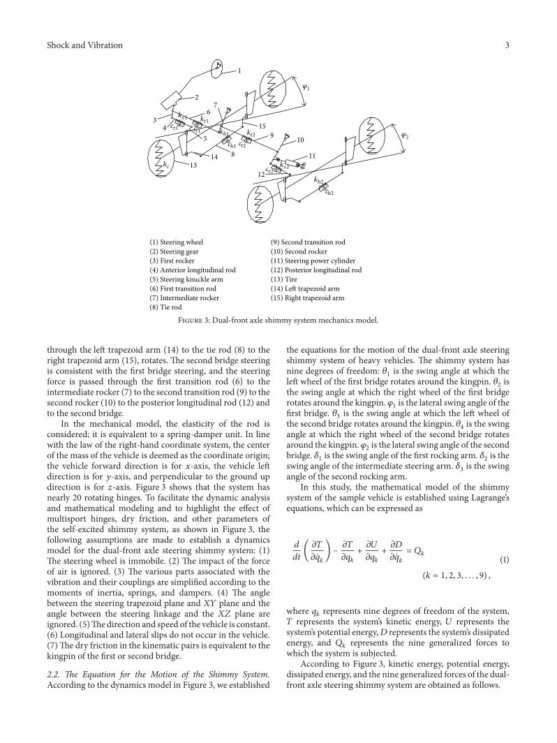
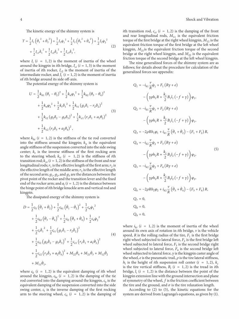
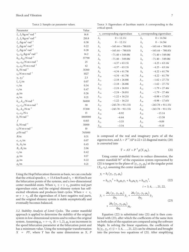
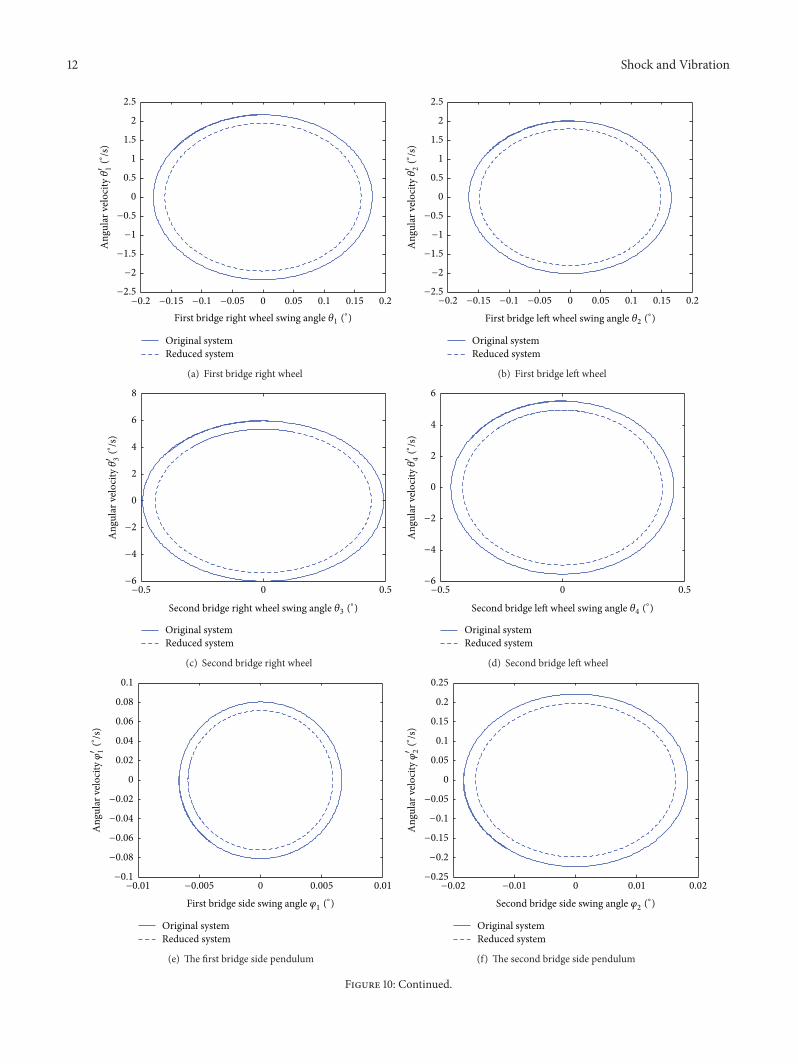
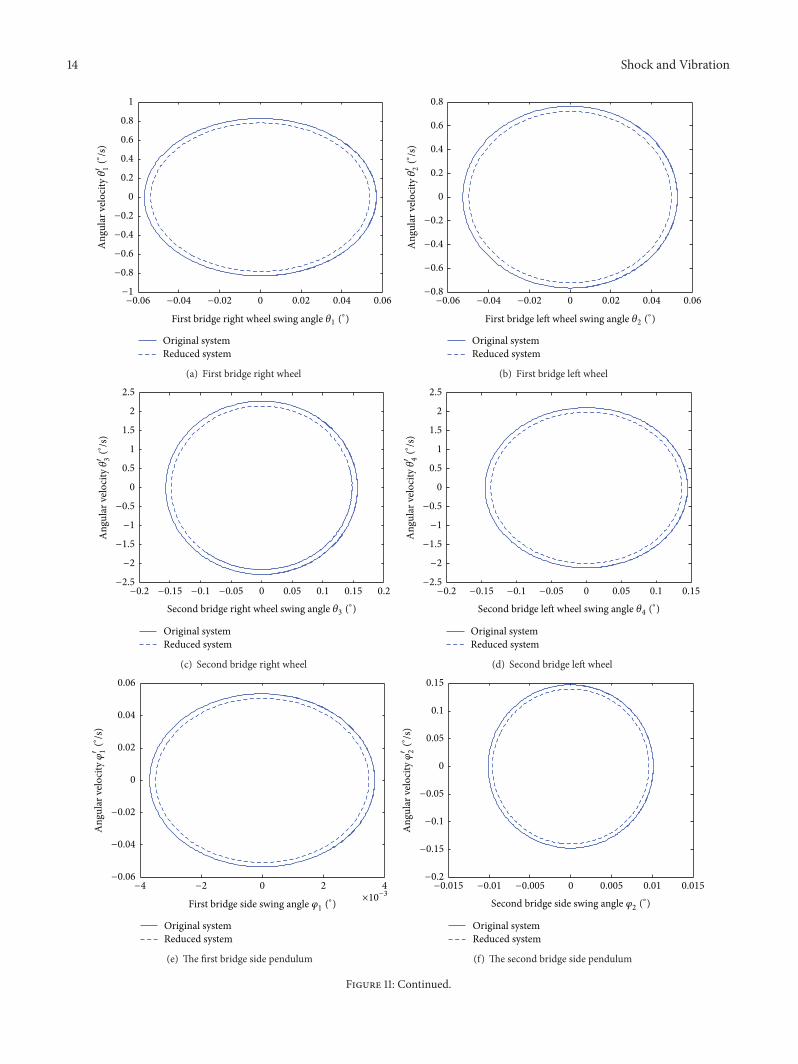

International Journal of
AerospaceEngineeringHindawi Publishing Corporationhttpwwwhindawicom Volume 2014
RoboticsJournal of
Hindawi Publishing Corporationhttpwwwhindawicom Volume 2014
Hindawi Publishing Corporationhttpwwwhindawicom Volume 2014
Active and Passive Electronic Components
Control Scienceand Engineering
Journal of
Hindawi Publishing Corporationhttpwwwhindawicom Volume 2014
International Journal of
RotatingMachinery
Hindawi Publishing Corporationhttpwwwhindawicom Volume 2014
Hindawi Publishing Corporation httpwwwhindawicom
Journal ofEngineeringVolume 2014
Submit your manuscripts athttpwwwhindawicom
VLSI Design
Hindawi Publishing Corporationhttpwwwhindawicom Volume 2014
Hindawi Publishing Corporationhttpwwwhindawicom Volume 2014
Shock and Vibration
Hindawi Publishing Corporationhttpwwwhindawicom Volume 2014
Civil EngineeringAdvances in
Acoustics and VibrationAdvances in
Hindawi Publishing Corporationhttpwwwhindawicom Volume 2014
Hindawi Publishing Corporationhttpwwwhindawicom Volume 2014
Electrical and Computer Engineering
Journal of
Advances inOptoElectronics
Hindawi Publishing Corporation httpwwwhindawicom
Volume 2014
The Scientific World JournalHindawi Publishing Corporation httpwwwhindawicom Volume 2014
SensorsJournal of
Hindawi Publishing Corporationhttpwwwhindawicom Volume 2014
Modelling amp Simulation in EngineeringHindawi Publishing Corporation httpwwwhindawicom Volume 2014
Hindawi Publishing Corporationhttpwwwhindawicom Volume 2014
Chemical EngineeringInternational Journal of Antennas and
Propagation
International Journal of
Hindawi Publishing Corporationhttpwwwhindawicom Volume 2014
Hindawi Publishing Corporationhttpwwwhindawicom Volume 2014
Navigation and Observation
International Journal of
Hindawi Publishing Corporationhttpwwwhindawicom Volume 2014
DistributedSensor Networks
International Journal of