Research Article Flexible Stock Allocation and Trim Loss ...

Research ArticleFlexible Stock Allocation and Trim Loss Control forCutting Problem in the Industrial-Use Paper Production

Fu-Kwun Wang and Feng-Tai Liu

Department of Industrial Management, National Taiwan University of Science and Technology, Taipei 106, Taiwan

Correspondence should be addressed to Fu-KwunWang; [email protected]

Received 29 November 2013; Accepted 25 May 2014; Published 17 June 2014

Academic Editor: Hsiao-Fan Wang

Copyright © 2014 F.-K. Wang and F.-T. Liu. This is an open access article distributed under the Creative Commons AttributionLicense, which permits unrestricted use, distribution, and reproduction in any medium, provided the original work is properlycited.

We consider a one-dimensional cutting stock problem (CSP) in which the stock widths are not used to fulfill the order but keptfor use in the future for the industrial-use paper production. We present a new model based on the flexible stock allocation andtrim loss control to determine the production quantity. We evaluate our approach using a real data and show that we are able tosolve industrial-size problems, while also addressing common cutting considerations such as aggregation of orders, multiple stockwidths, and cutting different patterns on the same machine. In addition, we compare our model with others, including trim lossminimization problem (TLMP) and cutting stock problem (CSP).The results show that the proposed model outperforms the othertwo models regarding total flexibility and trim loss ratio.

1. Introduction

A one-dimensional cutting stock problem (CSP) is one ofthe famous combinatorial optimization problems, which hasmany applications in industries, such as paper, wood, textiles,steel, space, ship construction, and logistic transportation[1–6]. Most studies focus on minimizing the trim loss thatis the amount of residual pieces of processed stock lengths.A standard one-dimensional cutting stock problem (S1D-CSP) as a kind of the above problems is known as an NP-complete one [7]. Numerous studies have examined how tofulfill orders and optimize production planning. Gilmore andGomory [8] presented a delayed pattern generation techniquefor solving a one-dimensional cutting problem using linearprogramming. Other methods, including pattern-orientedapproach, item-oriented approach,mixed approach and exactapproach, can be found in [9–27].

In the industrial-use paper industry, the productionquantity is usually greater than the customers’ order. Usingthe traditional CSP, the trim loss can be significant. Thus,we need to consider usable leftovers to prevent the trimloss generated after optimization. This issue becomes a one-dimensional CSP with usable leftovers. Yanasse [28] reportedthat the literature on usable leftovers is scarce and the

problem still lacks clear and appropriate definitions. Kos andDuhovnik [29] proposed usable leftover material used in thenext cutting plan to reduce trim loss. Related studies canbe found in [6, 29–35]. Cherri et al. [31] presented severalmodifications in some well-known heuristics to solve a one-dimensional CSP with usable leftovers. Poldi and Arenales[32] presented a study with the classical one-dimensionalinteger CSP, which consists of cutting a set of available stocklengths in order to produce smaller ordered items. Cui andYang [33] considered a one-dimensional CSP with usefulleftover in the cutting plan. Cherri et al. [35] proposed apriority-in-use heuristic approach to solve a one-dimensionalCSP with usable leftovers. However, these models cannotbe directly used for solving the CSP in the industrial-useproduction that each reel can only be produced a certainnumber of rolls depending on its cutting machine. Wang andLiu [36] presented a new decision model for reducing trimloss and inventory in the paper industry.

In this study, we present a new model based on theflexible stock allocation and trim loss control to determinethe production quantity. Our proposed model is a flexibilitymaximization problem (FAP). Under a certain conditionof trim loss control, FAP can be confined to cutting stockproblem (CSP) or trim loss minimization problem (TLMP).

Hindawi Publishing CorporationMathematical Problems in EngineeringVolume 2014, Article ID 521386, 9 pageshttp://dx.doi.org/10.1155/2014/521386

2 Mathematical Problems in Engineering

The remainder of this paper is organized as follows. InSection 2, the definition of problem in the paper industryis presented. A new model is developed in Section 3. InSection 4, some examples illustrate the application of theproposed model. Finally, conclusions are drawn in Section 5.

2. Problem Definition

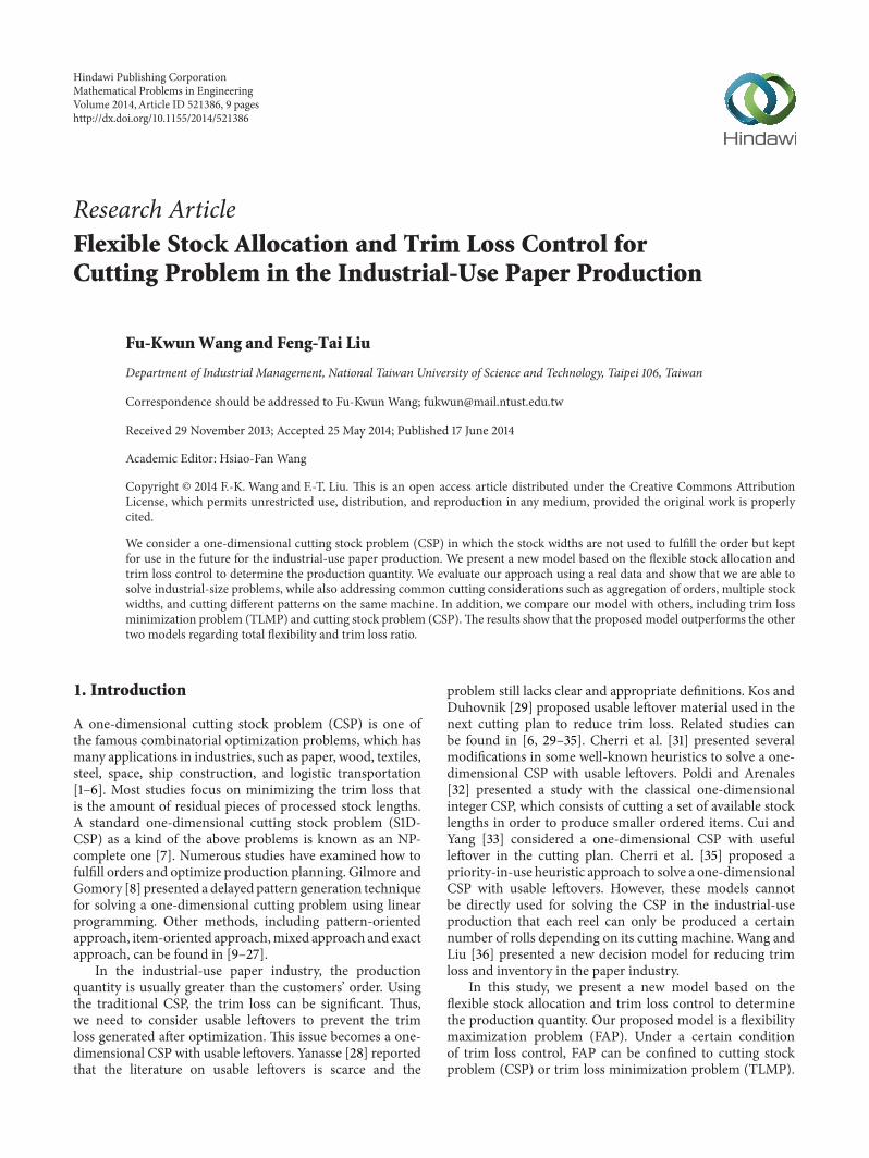
The production of industrial-use paper starts from rawmaterial to reels and then from reels to the productionof rolls as finished goods. The entire operation mode iscyclical production, which is the only method for achievingproduction efficiency. Therefore, the leftover material is notused in a follow-up production. For the production planning(see Figure 1), the customer’s paper requirements are obtainedand the marketing demand is predicted. Then, during thecombined production-marketing meeting, the number ofproduction days and the production quantity of paper typesare determined. The production quantity indicates the 𝑁

number of reels, and each reel can produce the NR number ofrolls that depends on the paper type. It should be noted thatthe unit of the paper width is millimeter (mm).

To formulate the models of CSP, TLMP and FAP, see thenotations section are used.

The main research question is how to improve the stockallocation and trim loss of a CSP with useful leftovers in thepaper industry.This problem can be studied for either one- ormultidimensional CSPs. In this study, one-dimensional CSPwith useful leftovers was used. We first provide two examplesto illustrate the differences between CSP, TLMP, and manualadjustment (MA). In practice, MA is used in the industrial-use paper industry in which the CSP and TLMP solutions arecandidates as manually selecting as MA solution. The CSPand TLMP are usually solved through column generation[8, 9]. To obtain the solutions ofCSP andTLMP, the computerprogram was written in Lingo 11 Software [37].

The formulation of CSP is defined as follows:

(CSP) Minimize𝑡

∑

𝑟=1

𝑥𝑟, (1)

s.t.

𝐿 ≥

𝑚

∑

𝑖=1

𝑎𝑖𝑟ow𝑖, (width of reel constraint)

(2)

𝑡

∑

𝑟=1

𝑎𝑖𝑟𝑥𝑟≥ 𝑑𝑖, (demand constraint) (3)

UB ≥ 𝐿 −

𝑚

∑

𝑖=1

𝑎𝑖𝑟ow𝑖, (trim loss constraint) , (4)

where 𝑎𝑖𝑟and 𝑥

𝑟are decision variables and integer variables.

Minimizing the total number of patterns is the objective func-tion (1) of the model. Constraint (2) guarantees the cuttingstocks regarding the reel width. Constraint (3) guarantees thecutting stocks regarding the demand. In the industrial-usepaper production, there exists the maximum trim loss for

each cutting, and then constraint (4) guarantees the waste ofeach roll during the cutting process.

In order to reduce the trim loss, a modified model calledTLMP is given as follows:

(TLMP) Minimize𝑡

∑

𝑟=1

(𝐿 −

𝑚

∑

𝑖=1

𝑎𝑖𝑟ow𝑖)𝑥𝑟, (5)

s.t.

𝐿 ≥

𝑚

∑

𝑖=1

𝑎𝑖𝑟ow𝑖, (width of reel constraint)

(6)

𝑡

∑

𝑟=1

𝑎𝑖𝑟𝑥𝑟≥ 𝑑𝑖, (demand constraint) (7)

SRQ =∑𝑡

𝑟=1𝑥𝑟

NR(reel set constraint) (8)

UB ≥ 𝐿 −

𝑚

∑

𝑖=1

𝑎𝑖𝑟𝑑𝑖, (trim loss constraint) ,

(9)

where 𝑎𝑖𝑟and 𝑥


Minimizing the total trim loss is the objective function(5) of the model. Constraint (6) guarantees the cuttingstocks regarding the reel width. Constraint (7) guaranteesthe cutting stocks regarding the demand. In industry paperproduction, the maximum trim loss for each cutting and thelimit production volume are considered; then constraint (8)guarantees the number of rolls for each reel, and constraint(9) guarantees the waste of each roll during the cuttingprocess.

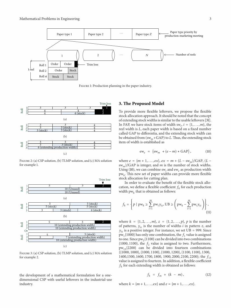
For example 1, we assume that the reel width is 10 units,NR is 3, UB is 3, the demand of order widths {3, 4} is {3, 3},and the stock widths are {3, 4, 5}. In Figure 2, we provideCSP, TLMP, and MA solutions. The trim loss using CSP is 5units. And the trim loss using TLMP is zero. We found thatthe stock width using CSP is obtained as {4} and the stockwidths using TLMP are {3} ∗ 3. In order to obtain flexiblestock widths, using MA based on CSP and TMLP solutions,the extending stock width is determined as {6}, and the stockwidth is obtained as {3}. Thus, MA can provide more flexiblestock width {6}.

For example 2, we assume that the reel width is 10 units,NR is 3, UB is 3, the demand of order widths {3, 5} is {1, 1},and the stock widths are {3, 4, 5}. In Figure 3, we provide CSP,TLMP, and MA solutions. The trim loss using CSP is 2 units.And the trim loss usingTLMP is zero.We found that the stockwidth using CSP is zero, the unused rolls are 2 and 3, and thestock widths using TLMP are {3} ∗ 1, {4} ∗ 1, and {5} ∗ 3.Using MA based on CSP and TMLP solutions, the extendingstock widths are determined as {10, 10} or {7, 10}, the stockwidth is obtained as zero or {5}, and the trim loss is obtainedas 2 units or zero. Thus, MA can provide more flexible stockwidths {10, 10} or {7, 10}.

Based on the above discussions, we conclude that theMA approach can provide more flexible stock widths in aone-dimensional CSP with useful leftovers. This motivates

Mathematical Problems in Engineering 3

Paper type priority by production-marketing meetingPaper type 1 Paper type 2 Paper type Z

1 2 N Number of reels

Order Order

Order Stock

Stock

Trim loss

Stock

Roll 1

Roll 2

Roll st

1 reel

· · ·

· · ·

Figure 1: Production planning in the paper industry.

1Trim loss

43

2

Roll 1

23 3

44 24 (stock)3

(a)

Roll 1

23 3 43 4

43 3 (stock) 3 (stock)3 (stock)

(b)

Roll 1

23 3 43 3 (stock) 4

6 (extending production width) 43

(c)

Figure 2: (a) CSP solution, (b) TLMP solution, and (c)MA solutionfor example 1.

Trim loss

5

Roll 1

2

2

10 (Unused)10 (Unused)

3

3

(a)

Roll 1

2

3 3 (stock) 4 (stock)5 (stock)5 (stock)

3

5

5 (stock)

(b)

Roll

Roll 5 (stock)

51

2

2

10 (extending production width)3

3 10 (extending production width)Or

1

2 3 7 (extending production width)3

5

10 (extending production width)

(c)

Figure 3: (a) CSP solution, (b) TLMP solution, and (c)MA solutionfor example 2.

the development of a mathematical formulation for a one-dimensional CSP with useful leftovers in the industrial-useindustry.

3. The Proposed Model

To provide more flexible leftovers, we propose the flexiblestock allocation approach. It should be noted that the conceptof extending stockwidths is similar to the usable leftovers [31].In FAP, we have stock items of width sw

𝑖, 𝑖 = {1, . . . , 𝑚}, the

reel width is 𝐿, each paper width is based on a fixed numbercalled GAP to differentia, and the extending stock width canbe obtained from (sw

𝑚+GAP) to 𝐿.Thus, the extending stock

item of width is established as

ew𝑒= {sw

𝑚+ (𝑒 − 𝑚) ∗ GAP} , (10)

where 𝑒 = {𝑚 + 1, . . . , 𝑒𝑥}, 𝑒𝑥 = 𝑚 + (𝐿 − sw𝑚)/GAP, (𝐿 −

sw𝑚)/GAP is integer, and 𝑚 is the number of stock widths.

Using (10), we can combine sw𝑖and ew

𝑒as production width

pw𝑘. This new set of paper widths can provide more flexible

stock allocation for cutting plan.In order to evaluate the benefit of the flexible stock allo-

cation, we define a flexible coefficient 𝑓𝑘for each production

width pw𝑘that is obtained as follows:

𝑓𝑘= {𝑝 | pw

𝑘≥

𝑚

∑

𝑖=1

pw𝑖𝑦𝑖𝑧,UB ≥ (pw

𝑘−

𝑚

∑

𝑖=1

pw𝑖𝑦𝑖𝑧)} ,

(11)

where 𝑘 = {1, 2, . . . , 𝑚}, 𝑧 = {1, 2, . . . , 𝑝}, p is the numberof patterns, 𝑦

𝑖𝑧is the number of widths 𝑖 in pattern 𝑧, and

𝑦𝑖𝑧is a positive integer. For instance, we set UB = 999. Since

pw1{1000} has only one combination, the𝑓

1value is assigned

to one. Since pw2{1100} can be divided into two combinations

{1000, 1100}, the 𝑓2value is assigned to two. Furthermore,

pw13{2200} can be divided into fourteen combinations

{{1000, 1000}, {1000, 1100}, {1000, 1200}, {1100, 1100}, 1300,1400,1500, 1600, 1700, 1800, 1900, 2000, 2100, 2200}; the 𝑓

13

value is assigned to fourteen. In addition, a flexible coefficient𝑓𝑘for each extending width is obtained as follows:

𝑓𝑘= 𝑓𝑚+ (𝑘 − 𝑚) , (12)

where 𝑘 = {𝑚 + 1, . . . , 𝑒𝑥} and 𝑒 = {𝑚 + 1, . . . , 𝑒𝑥}.


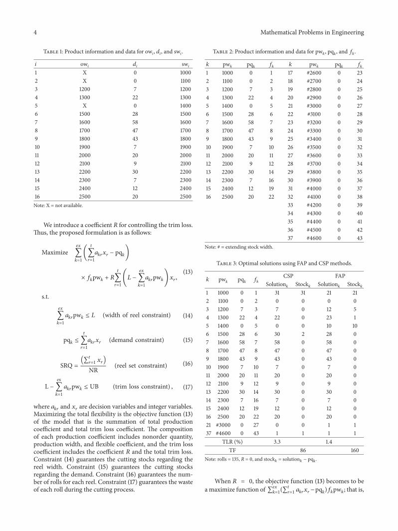
Table 1: Product information and data for ow𝑖, 𝑑𝑖, and sw

𝑖.

𝑖 ow𝑖

𝑑𝑖

sw𝑖

1 X 0 10002 X 0 11003 1200 7 12004 1300 22 13005 X 0 14006 1500 28 15007 1600 58 16008 1700 47 17009 1800 43 180010 1900 7 190011 2000 20 200012 2100 9 210013 2200 30 220014 2300 7 230015 2400 12 240016 2500 20 2500Note: X = not available.

We introduce a coefficient 𝑅 for controlling the trim loss.Thus, the proposed formulation is as follows:

Maximize𝑒𝑥

∑

𝑘=1

(

𝑡

∑

𝑟=1

𝑎𝑘𝑟𝑥𝑟− pq𝑘)

× 𝑓𝑘pw𝑘+ 𝑅

𝑡

∑

𝑟=1

(𝐿 −

𝑒𝑥

∑

𝑘=1

𝑎𝑘𝑟pw𝑘)𝑥𝑟,

s.t.

(13)

𝑒𝑥

∑

𝑘=1

𝑎𝑘𝑟pw𝑘≤ 𝐿 (width of reel constraint) (14)

pq𝑘≤

𝑡

∑

𝑟=1

𝑎𝑘𝑟𝑥𝑟

(demand constraint) (15)

SRQ =

(∑𝑡

𝑟=1𝑥𝑟)

NR(reel set constraint) (16)

L −ex∑

𝑘=1

𝑎𝑘𝑟pw𝑘≤ UB (trim loss constraint) , (17)

where 𝑎𝑘𝑟and 𝑥


Maximizing the total flexibility is the objective function (13)of the model that is the summation of total productioncoefficient and total trim loss coefficient. The compositionof each production coefficient includes nonorder quantity,production width, and flexible coefficient, and the trim losscoefficient includes the coefficient 𝑅 and the total trim loss.Constraint (14) guarantees the cutting stocks regarding thereel width. Constraint (15) guarantees the cutting stocksregarding the demand. Constraint (16) guarantees the num-ber of rolls for each reel. Constraint (17) guarantees the wasteof each roll during the cutting process.

Table 2: Product information and data for pw𝑘, pq𝑘, and 𝑓

𝑘.

𝑘 pw𝑘

pq𝑘

𝑓𝑘

𝑘 pw𝑘

pq𝑘

𝑓𝑘

1 1000 0 1 17 #2600 0 232 1100 0 2 18 #2700 0 243 1200 7 3 19 #2800 0 254 1300 22 4 20 #2900 0 265 1400 0 5 21 #3000 0 276 1500 28 6 22 #3100 0 287 1600 58 7 23 #3200 0 298 1700 47 8 24 #3300 0 309 1800 43 9 25 #3400 0 3110 1900 7 10 26 #3500 0 3211 2000 20 11 27 #3600 0 3312 2100 9 12 28 #3700 0 3413 2200 30 14 29 #3800 0 3514 2300 7 16 30 #3900 0 3615 2400 12 19 31 #4000 0 3716 2500 20 22 32 #4100 0 38

33 #4200 0 3934 #4300 0 4035 #4400 0 4136 #4500 0 4237 #4600 0 43

Note: # = extending stock width.

Table 3: Optimal solutions using FAP and CSP methods.

𝑘 pw𝑘

pq𝑘

𝑓𝑘

CSP FAPSolution

𝑘Stock

𝑘Solution

𝑘Stock

𝑘

1 1000 0 1 31 31 21 212 1100 0 2 0 0 0 03 1200 7 3 7 0 12 54 1300 22 4 22 0 23 15 1400 0 5 0 0 10 106 1500 28 6 30 2 28 07 1600 58 7 58 0 58 08 1700 47 8 47 0 47 09 1800 43 9 43 0 43 010 1900 7 10 7 0 7 011 2000 20 11 20 0 20 012 2100 9 12 9 0 9 013 2200 30 14 30 0 30 014 2300 7 16 7 0 7 015 2400 12 19 12 0 12 016 2500 20 22 20 0 20 021 #3000 0 27 0 0 1 137 #4600 0 43 1 1 1 1

TLR (%) 3.3 1.4TF 86 160

Note: rolls = 135, R = 0, and stock𝑘= solution

𝑘− pq𝑘.

When 𝑅 = 0, the objective function (13) becomes to bea maximize function of ∑𝑒𝑥

𝑘=1(∑𝑡

𝑟=1𝑎𝑘𝑟𝑥𝑟−pq𝑘)𝑓𝑘pw𝑘; that is,


Table 4: Optimal solutions using FAP and TLMP method.

𝑘 pw𝑘

pq𝑘

𝑓𝑘

TLMP FAPSolution

𝑘Stock

𝑘Solution

𝑘Stock

𝑘

1 1000 0 1 39 39 37 372 1100 0 2 2 2 1 13 1200 7 3 9 2 8 14 1300 22 4 22 0 23 15 1400 0 5 9 9 6 66 1500 28 6 28 0 28 07 1600 58 7 58 0 58 08 1700 47 8 47 0 47 09 1800 43 9 43 0 43 010 1900 7 10 7 0 7 011 2000 20 11 20 0 20 012 2100 9 12 9 0 9 013 2200 30 14 30 0 30 014 2300 7 16 7 0 7 015 2400 12 19 12 0 15 316 2500 20 22 20 0 20 0

TLR (%) 0.42 0.42TF 94 133

Note: rolls = 135, R = −1000, and stock𝑘= solution

𝑘− pq𝑘.

it does not consider trim loss. If the production capacity failsto satisfy (15) during the problem-solving process, a full rollis generated. Subsequently, because the flexibility of 𝑓

𝑒pw𝑒𝑥

is greater than any of the leniency and flexibility coefficientcombinations, the full roll is substituted by pw

𝑒𝑥. In addition,

the optimal CSP solution also generates a full roll and the fullroll is substituted by pw

𝑒𝑥; thus, the FAP results approximate

the CSP target function; that is, Minimize∑𝑡𝑟=1

𝑥𝑟. Therefore,

the difference between FAP(𝑅 = 0) and the 𝑎𝑘𝑟of CSP can

be compared.When R = −∞, ∑𝑒𝑥

𝑘=1(∑𝑡

𝑟=1𝑎𝑘𝑟𝑥𝑟− pq𝑘)𝑓𝑘pw𝑘can be

neglected and the objective function (13) approaches Maxi-mize 𝑅∑𝑡

𝑟=1(𝐿−∑

𝑒𝑥

𝑘=1𝑎𝑘𝑟pw𝑘)𝑥𝑟. In addition, 𝑅 approximates

the TLMP target function; that is, Minimize ∑𝑡

𝑟=1(𝐿 −

∑𝑒𝑥

𝑘=1𝑎𝑘𝑟pw𝑘)𝑥𝑟. Therefore, the difference between FAP(𝑅 =

−∞) and the 𝑎𝑘𝑟of TLMP can be compared.

In summary, when 𝑅 = 0, flexible stock becomes theoptimal condition and trim loss is maximized. Conversely,when 𝑅 = −∞, flexible stock becomes the least favorablecondition and trim loss is minimized. Therefore, the controlof variable 𝑅 is a flexible stock and trim loss strategy thatdecision makers adopt during the production process.

4. Illustrative Examples

We consider a real case from an industrial-use paper produc-tion and five simulated datasets to illustrate the application ofour proposedmethod.We set the current scheduling quantityas SRQ reels, and each reel can produce NR number of rolls.The cutting machine width limit is 𝐿, and the maximum trim

loss is UB. These parameters are defined as NR = 3, 𝐿 =

4600mm, SRQ = 45 reels = 135 rolls, and UB = 999mm.To obtain the solutions of CSP, TLMP, and FAP, the

computer program is divided into the engine and the userinterface. The engine interface was written in Lingo 11Software [37].The user interface in Visual Basic 5 enables thenavigation of data flow from various input sources, such as acommon company database and a random number dataset.

4.1. A Real Case from an Industrial-Use Paper Production.According to the FAP model in Section 3, the details are asfollows.

Step 1. Define ow𝑖,𝑑𝑖, and sw

𝑖, for 𝑖 = 1, 2, . . . , 16 (see Table 1).

Step 2. Using (10) to obtain the extending widths, sinceGAP = 100 and 𝑚 = 16, we can obtain that 𝑒 =

{17, 18, . . . , 37} and ew𝑒= {2600, 2700, . . . , 4600}.

Step 3. Aggregate 𝑑𝑖to pq𝑘, sw𝑖to pw

𝑘, and ew

𝑒to pw

𝑘, for

𝑖 = 1, 2, . . . , 16 and 𝑘 = 1, 2, . . . , 37.

Step 4. Use (11)-(12) to compute the flexible coefficient 𝑓𝑘for

pw𝑘(see Table 2).

Using FAP to perform optimization, 𝑅 must be set to 0,thereby allowing FAP results to approximate those of CSP. Inthis case, we obtained the production capacities of FAP andCSP, stock, trim loss ratio (TLR), and total flexible coefficient(TF), where TLR = [∑

𝑡

𝑟=1(𝐿 − ∑

𝑒𝑥

𝑘=1𝑎𝑘𝑟pw𝑘)𝑥𝑟]/(𝐿∑

𝑡

𝑟=1𝑥𝑟) ×

100% and TF = ∑𝑒𝑥𝑘=1

pw𝑘𝑓𝑘.

The primary reason for comparing CSP was to determinewhether FAP effectively reduced TLR and whether theflexible stock of FAP is superior to that of CSP (see Table 3).The TLRs for CSP and FAP were 3.3 and 1.4, respectively;the flexible stocks for CSP, FAP, and extending stock were{{1000, 31}, {1500, 2}, {#4600, 1}},{{1000, 21}, {1200, 5},{1300,1}, {1400, 10}, {#3000, 1}, {#4600, 1}}, and {{#3000, 1}, {#4600,1}}, respectively. Thus, the results suggest that FAPoutperforms CSP in reducing TLR and that the flexiblestock and TF of FAP are superior to that of CSP.

To compare FAP to TLMP, the flexible variable 𝑅 of FAPwas set to−1000, which denotesminimal TLR. In this case, weobtained the production capacities of FAP and TLMP, stock,TLR, and TF(see Table 4).

The primary reason for comparing TLMP was todetermine whether the TLR of FAP is similar to that of TLMPor not andwhether the flexible stock of FAP is superior to thatof TLMP or not (see Table 4). The TLRs for TLMP and FAPwere 0.42 and 0.42, respectively; the flexible stocks for TLMPand FAP were {{1000, 39}, {1100, 2}, {1200, 2}, {1400, 9}}, and{{1000, 37},{1100, 1}, {1200, 1}, {1300, 1}, {1400, 6}, {2400, 3}},respectively. Notably, the flexible stock of FAP {2400, 3} wasconsiderably more lenient. Therefore, based on the results,the TLR of FAP was identical to that of TLMP, and theflexible stock and TF of FAP were superior to those of TLMP.

Moreover, we employed sensitivity analysis to observethe influence that 𝑅 has on TLR and TF. When 𝑅 =

1, 0, −1, . . . , −∞, and 𝑅 is an integer, the results as shown inTable 5 are obtained.


Table 5: The sensitivity analysis of coefficient R for stock𝑘using FAP.

𝑘 pw𝑘

𝑓𝑘

𝑅

1 0 −1 ∼ −2 −3 ∼ −8 −9 ∼ −86 −87 ∼ −533 −534 ∼ −∞

1 1000 1 11 21 22 28 36 37 372 1100 2 0 0 1 1 1 1 13 1200 3 5 5 4 1 1 1 14 1300 4 1 1 1 1 1 1 15 1400 5 10 10 10 10 6 6 66 1500 6 0 0 0 0 0 0 07 1600 7 0 0 0 0 0 0 08 1700 8 0 0 0 0 0 0 09 1800 9 0 0 0 0 0 0 010 1900 10 0 0 0 0 0 0 011 2000 11 0 0 0 0 0 0 012 2100 12 0 0 0 0 0 0 013 2200 14 0 0 0 0 0 0 014 2300 16 0 0 0 0 0 0 015 2400 19 0 0 0 0 0 1 316 2500 22 0 0 0 0 0 0 021 #3000 27 1 1 1 1 1 0 037 #4600 43 1 1 1 1 1 1 0

TLR (%) 4.2 1.4 1.3 0.9 0.52 0.45 0.42TF 150 160 160 157 145 138 133

Note: the number of rolls = 135.

Table 6: The range and midpoint of R.

Range of R 0 −1 ∼ −2 −3 ∼ −8 −9 ∼ −86 −87 ∼ −533 −534 ∼ −∞

Midpoint 0 −1 −5 −47 −310 −1000

Table 7: Information of pq𝑘for simulated examples.

𝑘 pw𝑘

𝑓𝑘

Case1 2 3 4 5

1 1000 1 46 2 6 37 92 1100 2 3 15 2 47 413 1200 3 33 11 31 5 334 1300 4 22 21 22 42 275 1400 5 39 12 20 36 16 1500 6 46 25 6 31 27 1600 7 22 26 21 38 128 1700 8 34 21 34 6 419 1800 9 30 25 31 32 2910 1900 10 38 14 44 26 4811 2000 11 1 20 12 48 2212 2100 12 23 42 37 42 1613 2200 14 12 20 48 11 4814 2300 16 6 31 33 2 1915 2400 19 27 12 41 28 3016 2500 22 14 38 41 13 27

According to Table 5, when 𝑅 = 1, TLR increased and{1000, 21} changed to {1000, 11}. This was primarily because

Table 8: The results of TF and TLR for CSP, TLMP, and FAP.

Method Measure Case1 2 3 4 5

CSP TF 94 98 10 43 0TLR (%) 0 1.1 1.6 0.5 1.8

TLMP TF 49 19 6 10 9TLR (%) 0 0.15 1.2 0.13 1.2

FAP(R = 0)

TF 109 115 25 65 26TLR (%) 0 1 1.6 0.16 1.4

FAP(R = −1000)

TF 109 19 6 20 9TLR (%) 0 0.15 1.2 0.13 1.2

Rolls 144 141 183 162 162

trim loss was equivalent to the flexible coefficient of {1000},causing the stock capacity of {1000} to decrease. Thus, when0 ≤ 𝑅 < 1 is defined, we can directly use 𝑅 = 0 for solutionidentification.

When R < 0, we observed that the TF gradually reducedfrom 160 to 133 and the TLR reduced from 1.4 to 0.42.These results suggest that, when 𝑅 has a value less than 0,the TF decreases and the TLR declines. Regarding flexiblestock, we found that, when 𝑅 ranged between −1 and −2,


Table 9: Stock information for CSP, TLMP, and FAP.

Case Method Solution

1

CSP {1100, 1}{1500, 1}{#4600, 2}TLMP {1000, 3}{1100, 2}{2200, 3}

FAP (R = 0) {#2600, 1}{#4600, 2}FAP (R = −1000) {#2600, 1}{#4600, 2}

2

CSP {1000, 1}{2000, 1}{#4600, 2}TLMP {1000, 17}{1100, 1}

FAP (R = 0) {#3200, 1}{#4600, 2}FAP (R = −1000) {1000, 17}{1100, 1}

3

CSP {1300, 1}{1500, 1}

TLMP {1000, 6}

FAP (R = 0) {#2800, 1}FAP (R = −1000) {1000, 6}

4

CSP {#4600, 1}TLMP {1000, 6}{1300, 1}

FAP (R = 0) {2500, 1}{#4600, 1}FAP (R = −1000) {1000, 4}{1100, 1}{2200, 1}

5

CSP NATLMP {1000, 3}{1500, 1}

FAP (R = 0) {#2900, 1}FAP (R = −1000) {1000, 3}{1500, 1}

Note: {paper width, stock quantity}.

the production capacity of {1000} was 22; subsequently, as𝑅 decreased to between −3 and −8 and −534 and −∞, theproduction capacity of {1000} increased to 28 and to 37,respectively. These results suggest that, as 𝑅 decreases, theallocation of stock gradually coagulates at a lower leniency,negating the effects of extended stock. The decrease in TFfrom 160 to 133 implies that the degree of permitted flexibilityfor adjusting stock had already diminished. Therefore, wesuggest that𝑅 bemaintained within a range between −∞ and0.

Because the trim loss value at each interval of 𝑅 is a fixedvalue, we selected the medians of each interval and tabulatedthem into Table 6, which enabled us to select the desiredresults. Consequently, the number of medians can be definedby decision makers based on actual conditions.

4.2. Simulated Examples. To verify the superiority of theflexible stock and trim loss produced by using FAP overthose produced using CSP and TLMP, we selected 5 Casesfor comparison, and randomly obtained the pq

𝑘(where 𝑘 =

1, 2, . . . , 16), which was achieved by using the RANDBE-TWEEN function in Microsoft Office Excel 2007. The rangeof this function was set between 0, 1, 2, . . . , 50 (see Table 7).The optimization calculations were then performed for FAP,CSP, and TLMP.

We compared FAP(𝑅 = 0), FAP(𝑅 = −1000), CSP, andTLMP, and the results were tabulated in Table 8. Becauseusing FAP necessitates the consideration of the flexiblecoefficients, FAP(𝑅 = 0) should effectively reduce TLR whenan excessively large CSP’s TLR value is produced. Cases 2, 4,and 5 verified that FAP reduced CSP’s TLR. FAP(𝑅 = −1000)

and TLMP were then examined to determine whether FAP’sTLR presented similarities with TLMP’s TLR. Consequently,the TLR values observed in all the 5 Cases were consistent.

Subsequently, we endeavored to determine whether FAPcould effectively increase the flexibility of stock adjustment(see Table 9). The FAP(𝑅 = 0) for Cases 1 and 3 indicatedthat the stock leniency demonstrated a merging action. Inaddition, the extended stock was used in all of the casesamples. Furthermore, uncut rolls {#4600} were presented inCases 1, 2, 4, and 5. Because 𝑅 = 0 is the lowest productioncapacity model, this model is equivalent to CSP.The FAP(𝑅 =

−1000) for Cases 2, 3, and 5 was similar. However, FAP(𝑅 =

−1000) presented increased stock adjustment flexibility andextended stock usage in Cases 1 and 4. Thus, FAP(𝑅 = 0) caneffectively reduce CSP’s TLR and increase stock adjustmentflexibility when TLR is at a minimum level. The TLR inFAP(𝑅 = −1000) was equivalent to that of TLMP, whichincreased stock adjustment flexibility.

A sensitivity analysis was employed to determine theperformance of FAP in the 5 Cases and the influence of 𝑅on TLR and TF. Consequently, 𝑅 was set at 1, 0, −1, . . . , −∞,

where 𝑅 was an integer. The results are tabulated in Table 10.The medians tabulated in Table 6 were used for data

reconstruction and the results are presented in Table 11.Subsequently, we collected the 𝑅 values at each interval forCases 1, 3, 4, and 5. For Case 2, we were unable to collectthe 𝑅 values at intervals of −55–−79, −80–−124, and −125–−156. Decision makers can determine whether they wish toincorporate the medians at these intervals or not; however,this method of incorporating medians can be used to controlthe majority of TLR changes.

5. Conclusion

The results of the case study analysis indicate that FAP(𝑅 = 0)was similar to CSP in that both methods could be used todetermine theminimal production capacity and themaximal,flexible adjusted stock. Because of the unique productioncharacteristics of industrial-use paper, using the CSPmethodmay produce full rolls and, thus, cannot obtain optimizedtrim loss problems. Similar to the CSP method, FAP(𝑅 =

−1000) generates stock that cannot be flexibly adjusted,despite possessing minimal trim loss. Furthermore, CSP andTLMP failed to control the changes of TLR; therefore, FAPcan utilize 𝑅 to control and maintain TLR in a range betweenCSP and TLMP’TLR. This approach eliminates the trimloss problem exhibited in CSP and the adjustability problemexhibited in TLMP and allows decision makers to effectivelycontrol stock and trim loss according to actual situations.

Future research may consider solving extending stockin stock allocation. In addition, the cost effects during theproduction process should be addressed.

Notations

𝑖: The index number (𝑖 = 1, 2, . . . , 𝑚) and𝑚is the number of stock/order widths

sw𝑖: A stock width with 𝑖 = 1, 2, . . . , 𝑚

ow𝑖: An order width with 𝑖 = 1, 2, . . . , 𝑚


Table 10: The sensitivity analysis of coefficient R for all cases using FAP.

Case Measure R0 ∼ ∞

1 TLR (%) 0TF 109

0 ∼ −36 −37 ∼ −54 −55 ∼ −79 −80 ∼ −124 −125 ∼ −156 −157 ∼ ∞

2 TLR (%) 1 0.94 0.76 0.29 0.22 0.15TF 115 112 91 46 39 19

0 ∼ −19 −20 ∼ −∞

3 TLR (%) 1.6 1.2TF 25 6

0 ∼ −999 −1000 ∼ −∞

4 TLR (%) 0.16 0.13TF 65 20

0 ∼ −11 −12 ∼ −70 −71 ∼ −∞

5 TLR (%) 1.4 1.3 1.2TF 26 25 9

Table 11: The results of fixed values of R for all cases using FAP.

Case Measure R0 −1 −5 −47 −310 −1000

1 TLR (%) 0 0 0 0 0 0TF 109 109 109 109 109 109

2 TLR (%) 1 1 1 0.94 0.15 0.15TF 115 115 115 112 19 19

3 TLR (%) 1.6 1.6 1.6 1.2 1.2 1.2TF 25 25 25 6 6 6

4 TLR (%) 0.16 0.16 0.16 0.16 0.16 0.13TF 65 65 65 65 65 20

5 TLR (%) 1.4 1.4 1.4 1.3 1.2 1.2TF 26 26 26 25 9 9

𝑑𝑖: Demand for ow

𝑖with 𝑖 = 1, 2, . . . , 𝑚

𝐿: Reel widthNR: The number of rolls for a reelGAP: The difference between two paper widthsew𝑒: An extending production width, where 𝑒 is

the index number(𝑒 = 𝑚 + 1,𝑚 + 2, . . . , 𝑒𝑥) and𝑒𝑥 = 𝑚 + (𝐿 − sw

𝑚)/GAP

pw𝑘: A production width, where 𝑘 is the indexnumber (𝑘 = 1, 2, . . . , 𝑒𝑥)

pq𝑘: Quantity for the production width,𝑘 = 1, 2, . . . , 𝑒𝑥

𝑓𝑘: Flexible coefficient for the production

width pw𝑘, with 𝑘 = 1, 2, . . . , 𝑒𝑥

𝑅: Flexible coefficient for trim lossSRQ: Production scheduling of reel quantityUB: Upper bound for trim loss

𝑎𝑘𝑟: The number of widths 𝑘 in pattern 𝑟

𝑥𝑟: The number of patterns 𝑟, where 𝑟 is theindex number (𝑟 = 1, 2, . . . , 𝑡) and 𝑡 is thenumber of patterns.

Conflict of Interests

The authors declare that they have no conflict of interests.

References

[1] H. Stadtler, “A one-dimensional cutting stock problem in thealuminium industry and its solution,” European Journal ofOperational Research, vol. 44, no. 2, pp. 209–223, 1990.

[2] M. Gradısar, J. Jesenko, and G. Resinovic, “Optimization ofroll cutting in clothing industry,” Computers and OperationsResearch, vol. 24, no. 10, pp. 945–953, 1997.

[3] L. O. Morgan, A. R. Morton, and R. L. Daniels, “Simultaneouslydetermining the mix of space launch vehicles and the assign-ment of satellites to rockets,” European Journal of OperationalResearch, vol. 172, no. 3, pp. 747–760, 2006.

[4] G. Wascher, H. Haußner, and H. Schumann, “An improvedtypology of cutting and packing problems,” European Journalof Operational Research, vol. 183, no. 3, pp. 1109–1130, 2007.

[5] A. Dikili, A. Takinaci, and N. Pek, “A new heuristic approachto one-dimensional stock-cutting problems with multiple stocklengths in ship production,”Ocean Engineering, vol. 35, no. 7, pp.637–645, 2008.

[6] A. Abuabara and R. Morabito, “Cutting optimization of struc-tural tubes to build agricultural light aircrafts,” Annals ofOperations Research, vol. 169, no. 1, pp. 149–165, 2009.

[7] M. Gradisar, G. Resinovic, and M. Kljajic, “Evaluation of algo-rithms for one-dimensional cutting,” Computers & OperationsResearch, vol. 29, no. 9, pp. 1207–1220, 2002.

[8] P. C. Gilmore and R. E. Gomory, “A linear programmingapproach to the cutting-stock problem,” Operations Research,vol. 9, no. 6, pp. 849–859, 1961.


[9] P. C. Gilmore and R. E. Gomory, “A linear programmingapproach to the cutting stock problem, part II,” OperationsResearch, vol. 11, no. 3, pp. 863–888, 1963.

[10] W. Gochet and M. Vandebroek, “A dynamic programmingbased heuristic for industrial buying of cardboard,” EuropeanJournal of Operational Research, vol. 38, no. 1, pp. 104–112, 1989.

[11] C. H. Dagli, “Knowledge-based systems for cutting stockproblems,” European Journal of Operational Research, vol. 44,no. 2, pp. 160–166, 1990.

[12] H. Foerster and G. Wascher, “Simulated annealing for orderspread minimization in sequencing cutting patterns,” EuropeanJournal of Operational Research, vol. 110, no. 2, pp. 272–281, 1998.

[13] P. H. Vance, “Branch-and-price algorithms for the one-dimensional cutting stock problem,” Computational Optimiza-tion and Applications, vol. 9, no. 3, pp. 211–228, 1998.

[14] M. Gradisar, M. Kljajic, G. Resinovic, and J. Jesenko, “Asequential heuristic procedure for one-dimensional cutting,”European Journal of Operational Research, vol. 114, no. 3, pp.557–568, 1999.

[15] M. Sakawa, I. Nishizaki, and M. Hitaka, “Interactive fuzzy pro-gramming for multi-level 0-1 programming problems throughgenetic algorithms,” European Journal of Operational Research,vol. 114, no. 3, pp. 580–588, 1999.

[16] S. M. A. Suliman, “Pattern generating procedure for the cuttingstock problem,” International Journal of Production Economics,vol. 74, no. 1–3, pp. 293–301, 2001.

[17] H. B. Amor, J. Desrosiers, and J. M. Valerio de Carvalho,“Dual-optimal inequalities for stabilized column generation,”Operations Research, vol. 54, no. 3, pp. 454–463, 2006.

[18] P. Trkman and M. Gradisar, “One-dimensional cutting stockoptimization in consecutive time periods,” European Journal ofOperational Research, vol. 179, no. 2, pp. 291–301, 2007.

[19] W.-C. Weng and T.-C. Sung, “Optimization of a line-cuttingprocedure for ship hull construction by an effective tabu search,”International Journal of Production Research, vol. 46, no. 21, pp.5935–5949, 2008.

[20] C. Alves and J. M. Valerio de Carvalho, “Accelerating columngeneration for variable sized bin-packing problems,” EuropeanJournal of Operational Research, vol. 183, no. 3, pp. 1333–1352,2007.

[21] S. L. Nonas and A. Thorstenson, “Solving a combined cutting-stock and lot-sizing problem with a column generating proce-dure,” Computers and Operations Research, vol. 35, no. 10, pp.3371–3392, 2008.

[22] H. Reinersten and T. W. M. Vossen, “The one-dimensionalcutting stock problem with due dates,” European Journal ofOperational Research, vol. 201, no. 3, pp. 701–711, 2010.

[23] K. Matsumoto, S. Umetani, and H. Nagamochi, “On the one-dimensional stock cutting problem in the paper tube industry,”Journal of Scheduling, vol. 14, no. 3, pp. 281–290, 2011.

[24] J. Erjavec, M. Gradisar, and P. Trkman, “Assessment of stocksize to minimize cutting stock production costs,” InternationalJournal of Production Economics, vol. 135, no. 1, pp. 170–176,2012.

[25] M. H.M. A. Jahromi, R. Tavakkoli-Moghaddam, A.Makui, andA. Shamsi, “Solving an one-dimensional cutting stock problemby simulated annealing and tabu search,” Journal of IndustrialEngineering International, vol. 8, no. 1, pp. 24–31, 2012.

[26] A. Mobasher and A. Ekici, “Solution approaches for the cut-ting stock problem with setup cost,” Computers & OperationsResearch, vol. 40, no. 1, pp. 225–235, 2013.

[27] G. C. Wang, C. P. Li, J. Lv, X. X. Zhao, and H. Y. Cuo, “Anefficient algorithm design for the one-dimensional cutting-stock problem,” Advanced Materials Research, vol. 602–604, pp.1753–1756, 2013.

[28] H. H. Yanasse, “A review of three decades of research on somecombinatorial optimization problems,” Pesquisa Operacional,vol. 33, no. 1, pp. 11–36, 2013.

[29] L. Kos and J. Duhovnik, “Cutting optimization with variable-sized stock and inventory status data,” International Journal ofProduction Research, vol. 40, no. 10, pp. 2289–2301, 2002.

[30] S.Dimitriadis andE.Kehris, “Cutting stock optimization in cus-tom door and window manufacturing industry,” InternationalJournal of Decision Sciences, Risk and Management, vol. 1, no. 1,pp. 66–80, 2009.

[31] A. C. Cherri, M. N. Arenales, and H. H. Yanasse, “The one-dimensional cutting stock problem with usable leftover—aheuristic approach,” European Journal of Operational Research,vol. 196, no. 3, pp. 897–908, 2009.

[32] K. C. Poldi and M. N. Arenales, “Heuristics for the one-dimensional cutting stock problem with limited multiple stocklengths,” Computers and Operations Research, vol. 36, no. 6, pp.2074–2081, 2009.

[33] Y. Cui and Y. Yang, “A heuristic for the one-dimensionalcutting stock problem with usable leftover,” European Journalof Operational Research, vol. 204, no. 2, pp. 245–250, 2010.

[34] S. A. Araujo, A. A. Constantino, and K. C. Poldi, “An evolution-ary algorithm for the one-dimensional cutting stock problem,”International Transactions in Operational Research, vol. 18, no.1, pp. 115–127, 2011.

[35] A. C. Cherri, M. N. Arenales, and H. H. Yanasse, “The usableleftover one-dimensional cutting stock problem—a priority-in-use heuristic,” International Transactions in OperationalResearch, vol. 20, no. 2, pp. 189–199, 2013.

[36] F. K. Wang and F. T. Liu, “A new decision model for reducingtrim loss and inventory in the paper industry,” Journal of AppliedMathematics, vol. 2014, Article ID 987054, 10 pages, 2014.

[37] Lingo Software, Version 11, Lindo Systems, Inc, Chicago, Ill,USA, 2009.

Submit your manuscripts athttp://www.hindawi.com

Hindawi Publishing Corporationhttp://www.hindawi.com Volume 2014

MathematicsJournal of


Mathematical Problems in Engineering

Hindawi Publishing Corporationhttp://www.hindawi.com

Differential EquationsInternational Journal of

Volume 2014

Applied MathematicsJournal of


Probability and StatisticsHindawi Publishing Corporationhttp://www.hindawi.com Volume 2014

Journal of


Mathematical PhysicsAdvances in

Complex AnalysisJournal of


OptimizationJournal of


CombinatoricsHindawi Publishing Corporationhttp://www.hindawi.com Volume 2014

International Journal of


Operations ResearchAdvances in

Journal of


Function Spaces

Abstract and Applied AnalysisHindawi Publishing Corporationhttp://www.hindawi.com Volume 2014

International Journal of Mathematics and Mathematical Sciences


The Scientific World JournalHindawi Publishing Corporation http://www.hindawi.com Volume 2014


Algebra

Discrete Dynamics in Nature and Society



Decision SciencesAdvances in

Discrete MathematicsJournal of

Hindawi Publishing Corporationhttp://www.hindawi.com

Volume 2014 Hindawi Publishing Corporationhttp://www.hindawi.com Volume 2014

Stochastic AnalysisInternational Journal of

Research Article Flexible Stock Allocation and Trim Loss ...

Documents

Transcript of Research Article Flexible Stock Allocation and Trim Loss ...