Research Article Fashion Brand Purity and Firm...

Hindawi Publishing CorporationMathematical Problems in EngineeringVolume 2013 Article ID 363095 18 pageshttpdxdoiorg1011552013363095

Research ArticleFashion Brand Purity and Firm Performance

Jin-hui Zheng1 Zixia Cao2 Xin Dai3 and Chun-Hung Chiu3

1 Institute of Textiles and Clothing The Hong Kong Polytechnic University Hung Hom Kowloon Hong Kong2Department of Management Marketing and General Business West Texas AampM University Canyon TX 79016 USA3 Sun Yat-Sen Business School Sun Yat-Sen University No 135 Xingang West Road Guangzhou 510275 China

Correspondence should be addressed to Xin Dai daixinmailsysueducn

Received 7 December 2012 Accepted 12 February 2013

Academic Editor Tsan-Ming Choi

Copyright copy 2013 Jin-hui Zheng et al This is an open access article distributed under the Creative Commons Attribution Licensewhich permits unrestricted use distribution and reproduction in any medium provided the original work is properly cited

A large number of prior empirical research and case studies used qualitative methodology to discuss the fashion brand dilutionresulting from consumer base extension from the target group(s) to the nontarget groups and its impacts From a differentperspective this paper establishes a dynamic brand dilution and performance model demonstrating how dynamic changes of salesvolumes involving the two consumer groups affect the degree of brand dilution and the performance of the brand We incorporatethe factor ldquobrand purityrdquo to the model as a quantitative measure of brand dilution level that affects firm annual revenue and profitchange comprehensively in iteration Our model suggests that fashion brands especially luxury brands can be easily diluted underthe pressure of firm growth and the brands suffer the significant negative impact on their revenues and profit While increasingsales volume can aggravate the negative consequences brand purity can be increased through limiting the consumer base to thetarget group only

1 Introduction

The challenge faced by many fashion brands is that whetherto stay within the existing target market to avoid branddilution or to extend the brand to a larger market with therisks of diluting the brand [1] Increasing consumer baseseems to facilitate firm growth but prior research found thatconsumers tend to value the product (or the brand) less whena larger group of consumers owns it [2] Because consumersrsquodecision to buy a ldquoconspicuousrdquo branded product dependson not only the productrsquos functionality but also the brandrsquossocial benefits such as its prestige [2ndash6] the fashion brandneeds to maintain its exclusivity A brand is no longer worthits vertiginous price if it is owned by too many consumers [7]

We have witnessed the failures of excessivemarket expan-sions where some fashion brands were diluted Lacoste awell-established French high-end apparel brand was popularamong many young people in the poorly developed outersuburban area of African The expanded market segmentof Lacoste conflicted with its brand positioning [7] Thecompanyrsquos advertising manager Didier Calon viewed thephenomenon during an interview in 2005 ldquoIt obviously had

negative effects on the brand image Certain of our consumerswere upset that we could pursue this target when in factwe have no control over it Our sales decreased for threeor four years rdquo [8] The classic high-end British brandBurberry became popular with the British football casualcult during the 1970s leading it to be associated with chavshooligans and members of football companies by the 1990sEven Burberry admitted that ldquoBurberry is now synonymouswith chavs and thugsrdquo at that time [9] To revitalize thebrand Burberry spent a huge amount of resources on theadvertising campaign [10] Pierre Cardin is another exampleof the fashion brand that overextended the market at thecost of degrading its brand value and losing shares in itsprimary target market Pierre Cardinrsquos licensing operationsproliferated so much that the name had been lent to morethan 800 products by the 1980s including toilet-seat coversIn the end despite his talents as a couturier his name becametoo common for many high-fashion consumers [11] A recentrelevant observation is that when Louis Vuitton hired his newCEO who was formerly executive vice president of Frenchfood giantrsquos division in the end of 2012 lots of connoisseursworried that the management change provides a hint of

2 Mathematical Problems in Engineering

its plan of entering the mass market that could dilute LVbrand These phenomena are known as ldquobrand dilutionrdquoreferring to the weakening of a brand due to its overuseBrand dilution frequently happens as a result of unsuccessfulbrand extension [12ndash14]

Price cutting might increase sales volume but might alsodamage brand equity [11] Brand extension which extends theoriginal brand to the newmarkets could exert dilution effectson the parent brand when the attributes of extended brandsare inconsistent with the original brand positioning [1 15ndash17]Many related studies in fashion industry explained why somefactors are critical for brand extension success [18ndash20] Thispaper focuses on expanding the customer base to nontargetconsumers by cutting priceThis brand dilution factor resultsfrom social influences such as conspicuous consumption [23 11 20]

Han et al [21] demonstrate with field experiments andmarket data that a market segmentrsquos preference for con-spicuously (or inconspicuously) branded luxury product issignificantly related with consumersrsquo desire to be associatedor dissociated with the members of that segment Priorstudies have identified two competing social needs amongconsumers a need for uniqueness and a countervailing needfor conformity [22 23] Research in the area of referencegroup suggests the differences between consumer groupsFor example consumers from the elite group would liketo distinguish themselves from the masses in consumptionbut the masses seek to emulate the choices of the elites [2425] Therefore we build the model based on two groups ofconsumers namely the leader-group (LG) consumers andthe follower-group (FG) consumers LG consumers seek forthe uniqueness and devalue a brand owned by too many FGwhereas FG consumers would like to follow LG and makethe purchasing decisions when prices are acceptable [7 26]Assuming that the fashion firm can change sales volume byadjusting product prices we expect that the demand from FGwill be increased when price is lowered A higher demand ofLG induces a higher demand of FG while a higher demandof FG leads to a lower demand of LG

The impact of brand dilution on firm performance iswidely observed and discussed [12 27 28] especially infashion industry [29] Some empirical studies measured theindexes of brand dilution and its moderating effect [13 14 3031] Here we use the concept of brand purity to denote thedegree of brand dilution that is defined in the mathematicmodel

While many cases suggest the essential tradeoff thatfashion brands need to make between increasing marketshare and degrading brand value there is little research thathas analyzed the dynamic mechanism of brand dilutionTherefore we establish a dynamic brand dilution model andinvestigate analytically and numerically the situations wherebrand dilution occurs the effects of brand dilution on brandfirm performance and the strategies to cope with branddilution The findings provide managerial implications forfashion firms regarding how to achieve the balance betweenmarket extension and brand dilution to optimize the firmperformance

119875

119902lowast

IIIIII

119876119902

119875

119902

Figure 1 Demand curve and sales revenue

For the numerical analysis we use the System Dynamics(SD) that is a widely used methodology and mathematicalmodeling technique that clearly visualizes the model Byusing SD model the dynamic brand dilution model is vividand is easier to understand In addition SD model is suitableto conduct stimulation for a particular case and to produceiteration results It also acts as a delicate what-if tool formanagers to conveniently modify specific variables of themodel based on their needs and observe stimulation resultsunder different conditions

This paper contributes to the literature by (1) firstintroducing the idea of the brand purity and proposing aquantitative measure of brand dilution level (2) establishingthe dynamic brand dilution model and (3) demonstratinganalytically and numerically how dynamic changes of salesvolumes affect the brand purity and the firm performance

We develop an economic model for the mechanism ofbrand dilution in Section 2 and analyze the process of howbrand dilution and firm performance develops in Section 3The related system dynamics model and the numerical anal-ysis appear in Section 4 Simulations on luxury fashion brandbackground further validate the process of brand dilution inSection 5 Conclusions are summarized in Section 6

2 Model

21 Price-Sales Volume Relation To simplify the configu-ration we use demand curves to describe the relationshipbetween the selling price and the quantity (sales volume)of a fashion brand in Figure 1 Given the existing productportfolio of the fashion brand let 119901 be the highest price ofthe branded products within the product portfolio and 119902

the corresponding sales volume of these products Within acertain period price will be arbitrarily modified to adapt tothe market thus gradually falling below the starting price 119901Let 119901 = 119901(119902) where 119901 gt 0 119902 gt 0 119889119901119889119902 lt 0 11988921199011198891199022 ge 0 bethe price function The price function indicates that the finalsale volume is 119902 if the final retail price is set at 119901(119902) The firmcan reduce price to boost sales

The revenue of the fashion brand is calculated by accu-mulating the product of the price and the quantity on thedemand curve for example if the final price is 119901(119902) thenthe revenue of all the goods with 100 brand purity (thedefinition of brand purity and its effects on revenue arediscussed later in this section) is given by the sum of areasI II and III in Figure 1

Mathematical Problems in Engineering 3

Price can effectively distinguish LG and FG consumers ofthe fashion brand [32] For simplicity we assume 119901lowast is thecutoff price for distinguishing these two types of consumersthat is LG consumers only purchase the product of the brandwhen 119901 gt 119901

lowast and FG consumers only purchase the productof the brandwhen119901 le 119901lowast where119901lowast = 119901(119902lowast)The cutoff price119901

lowast between LG and FG is rational simplification to reality inwhichLGandFGcould have their own affordable price spansand the two price spans can be overlapped or isolated Notethat 119902lowast is called the ldquocritical pointrdquo of the sales volume thatdifferentiates LG consumers and FG consumers

Although brands can set price to control the sales volumeit is still difficult for them to prevent brand dilution becausethey might not actually discern what is the exact 119902lowast and areeasy tomake actual sales volume bigger than the unknown 119902lowast(the lowest price is set lower than 119901lowast) where FG consumersare involved and brand dilution occurs

22 Brand Purity The brand purity represents the mix ofconsumer amongst consumer groups Let 119902

119871be the sales

volume of LG consumers and 119902

119865the sales volume of FG

consumers The total sales volume is given by 119902 = 119902

119871+ 119902

119865

Let 119904 be the brand purity We consider that the brand is purewith 119904 = 1 when only LG consumers purchase the productsof the brand and the brand is diluted with 119904 lt 1 whenFG consumers also purchase the products of the brand tooThe smaller the 119904 is the more the FG consumers purchasethe products and the more the brand is diluted Noting thatthe measure of the brand purity 119904 can be defined in manyways 119904 = 119902

119871(119902

119871+ 119902

119865) is a simple example of the measure

However it does not reflect the dynamic feature of the brandpurity so we do not adopt this measure A dynamic brandpuritymeasure is introduced in Section 23 later in this paperThe brand purity affects the purchasing intension of the LGconsumers (but does not affect the purchasing intension ofthe FG consumers) For simplicity we consider that for 0 le119904 le 1 only 119904 portion of the demand of LG consumers will betransformed into the sales volume of the brand products

For any given 0 le 119904 le 1 and the final price 119901(119902) therevenue of the brand for one selling season is given by

119877 = 119901 (119902) 119902119904 + int

119902

119902

119901 (119902) 119904119889119902 for 119902 le 119902lowast (1a)

119877 = 119901 (119902) 119902119904 + int

119902lowast

119902

119901 (119902) 119904119889119902 + int

119902

119902lowast

119901 (119902) 119889119902 for 119902 gt 119902lowast

(1b)

where 119901(119902)119902 is area I in Figure 1 int119902119902119901(119902)119889119902 is the front part of

area II (for 119902 le 119902lowast) int119902lowast

119902119901(119902) is area II in Figure 1 (for 119902 gt 119902lowast)

and int119902119902lowast119901(119902)119889119902 is III in Figure 1 (for 119902 gt 119902

lowast) Moreover theprofit of the brand for one selling season is given by

119874 = (119901 (119902) minus 119888) 119902119904 + int

119902

119902

(119901 (119902) minus 119888) 119904119889119902 minus 119862 for 119902 le 119902lowast

(2a)

119874 = (119901 (119902) minus 119888) 119902119904 + int

119902lowast

119902

(119901 (119902) minus 119888) 119904119889119902 minus 119862

+ int

119902

119902lowast

(119901 (119902) minus 119888) 119889119902 minus 119862 for 119902 gt 119902lowast(2b)

where 119888 is the variable cost and119862 is the fixed cost of the brand

23 Dynamic Model In this paper we consider a multipleselling season situation (for simplicity we consider 1 yearfor 1 selling season) In each year the brand will pushnew products to the market Denote by 119904

119894 119877119894 and 119874

119894(we

use subscript to represent the year for all other notations)respectively the brand purity the revenue and the profit ofthe brand in the 119894th year which are included where 119894 is anonnegative integer We consider the dynamics model of thebrand purity as follows

119904

119894= 120572119904

119894minus1+ (1 minus 120572)

119902

119871119894

119902

119894

119904

0= 1 (3)

where 0 lt 120572 lt 1 119902119871119894

is the sales volume of LG consumersin 119894th year and 119902

119894is the total sales volume of both LG

and FG consumers By noting the dynamic brand purity (3)follows the format of exponential weighted moving average(EWMA) that is 119904

119894is the weighted sum on the last brand

purity status 119904119894minus1

and the current mix of the sales volume ofthe two groups of consumers 119902

119871119894119902

119894We set 119904

0= 1 and assume

that there is no brand dilution at the beginning Starting fromthe 1st year the brand dilution begins when FG consumersstart to purchase this brand Let 119902

119865119894be the sales volume of

FG consumers in the 119894th year By following (3) the degree ofbrand purity is accumulated from year 0 up to year 119894 minus 1

By following (1b) the revenue of the brand in year 119894 is

119877

119894= 119901 (119902) 119902119904

119894minus1+ int

119902lowast

119902

119901 (119902) 119904

119894minus1119889119902

+ int

119902119894+(1minus119904

119894minus1)119902lowast

119902lowast

119901 (119902) 119889119902 for 119901119894lt 119901 (119902

lowast)

(4)

In (4) the base of LG consumers of year 119894 shrinks by anamount proportional to the brand purity 119904

119894minus1 As 119902119871119894= 119904

119894minus1119902

lowast

and 119902119865119894= 119902

119894minus119904

119894minus1119902

lowast when 119901 lt 119901lowast the final price will declineto 119901(119902

119894+(1minus119904

119894minus1)119902

lowast) = 119901(119902

lowast+119902

119865119894) to obtain 119902

119865119894sales volume

from FG Moreover the annual profit of the brand is given by

119874

119894= (119901 (119902) minus 119888) 119902119904

119894minus1+ int

119902lowast

119902

(119901 (119902) minus 119888) 119904

119894minus1119889119902

+ int

119902119894+(1minus119904


119902lowast

(119901 (119902) minus 119888) 119889119902 minus 119862 for 119901119894lt 119901 (119902

lowast)

(5)

When the fashion brand wants to achieve more annualrevenue and profit through lowering the price to enlargethe sales volume brand dilution which will undermine thefirm performance (revenue and profit) occurs once the salesvolume exceeds the critical point 119902lowast and FG consumers areattracted to the brand


3 Analysis

The increase of sales volume of the fashion brand is oftenconsidered as an indicator of brand growth Under thepressure from the stakeholders the brand is highly motivatedto continue increasing its sales volume overtime Although toincrease the sales volume the brand has to decrease marginalprice it still has plenty of space to cut prices as the priceof fashion product is usually significantly higher than theproduct cost The growth mechanisms of brands with a purebrand (119904 = 1) and with diluted brand (119904 lt 1) are different aswe discuss below

31 The Brand Is Pure When the brand is pure increasingsales volume is a good strategy for a firm to enjoy continuedincreasing revenue and profit

Proposition 1 Suppose that 119904119894minus1

= 1 119904119894lt 1 only if sales

volume 119902119894gt 119902

lowast (or 119901119894le 119901(119902

lowast)) (All proofs are presented in

Appendix A)

Discussion of Proposition 1 As shown in Proposition 1 dilu-tion does not occur when only LG consumers purchase theproducts or dilution occurs until FG consumers start topurchase the brand


= 1 if 119904119894= 1 119877

119894and 119874

119894are

both increasing functions of 119902

Discussion of Proposition 2 As the maximum 119902 that keepsthe brand pure is 119902

lowast (by Proposition 1) according toProposition 2 the revenue and the profit of the brand aremaximized at 119902 = 119902

lowast when the brand is pure and cuttingprice to increase sales (less than 119902lowast) volume leads to positiveconsequences (higher revenue and profit) over years

32 The Brand Is Diluted Once the firm gets used to theexperience of benefiting from increasing sales volume thefirm may have the tendency to oversell the products to FGconsumers and suffer the negative impacts of brand dilutionTo focus on brand dilution effects our analysis starts from thecritical point of brand dilution Moreover for simplicity weassume that the fashion brand firmwill increase sales volumeat an annual rate of 120579

119894gt 0 Hence the sales volume in year 119894

is given by

119902

119894= 119902

lowast

119894

prod

119895=1

(1 + 120579

119895) 119902

0= 119902

lowast (6)

Following the changes in sales volume the brandpurity is alsoaltered

119904

119894= 120572119904

119894minus1+ (1 minus 120572)

119902

119871119894

119902

119894

= 120572119904

119894minus1+ (1 minus 120572)

119902

lowast119904

119894minus1

119902

lowastprod

119894

119895=1(1 + 120579

119895)

= (120572 +

1 minus 120572

prod

119894

119895=1(1 + 120579

119895)

) 119904

119894minus1

(7)

or

119904

119894=

119894

prod

119896=1

(120572 +

1 minus 120572

prod

119896

119895=1(1 + 120579

119895)

) (8)

According to (8) 119904119894will decrease at an accelerating rate of

(120572+ (1minus120572)(1 + 120579)

119894) namely the brand purity will be eroded

severely as the sales volume continues to rise The brand willgradually lose its superiority to LG consumerswho contributethe majority of its revenue inevitably resulting in a shrinkingof LG consumer base

Proposition 3 If 1199040= 1 and 119904

119894is given by (8) with 120579

119894gt 0

119894 = 1 2 then 119904119894+2119904

119894+1lt 119904

119894+1119904

119894lt 1

Discussion of Proposition 3 Once the increasing sale volumeexceeds the critical point 119902lowast and the brand purity declinesthe process of brand dilution will accelerate as sales volumekeeps increasing So things will deteriorate swiftly whenbrand dilution happens Is there anything we can do for itFor example to keep the annual sales volume unchanged afterbrand dilution occurs let119867 gt 1 be an integer

Proposition 4 Suppose that 120579119896gt 0 for 119896 = 1 119867 minus 1 and

120579

119896= 0 for 119896 ge 119867 If 119904

119894is given by (8) then 119904

119894+2119904

119894+1= 119904

119894+1119904

119894lt

1 for 119894 gt 119867

Discussion of Proposition 4 Once the brand purity starts todecline stopping increasing the sales volume cannot preventthe deterioration and the brand purity will still decrease at aconstant rate This case is a little bit better than decreasing atan accelerating rate but is still bad because it cannot stop thebrand to ruin So how about cutting the sales volume after thebrand is diluted

Proposition 5 119904119894ge 119904

119894minus1 119894 isin 119873 if and only if 119902

119894le 119902

lowast

Discussion of Proposition 5 Once the brand purity declinesthe firm can enhance brand purity by reducing sales lessthan 119902

lowast Noting that sales volume is less than 119902

lowast does notimply all the sales volume is made up of LG consumersespecially fashion brand which had ever diluted To enhancebrand image sales volume of current year should be confinedwithin the range In other words only cutting sales volumea little cannot promise improving the brand purity when italready exceeds the critical point 119902lowast Therefore brand puritywill continue to decline unless sales volume decreases tobelow 119902

lowast However in practice recovering a diluted brand isalways difficult because firms are often reluctant to adopt suchradical method Moreover Proposition 5 once again showsthe importance of the critical point 119902lowast No matter how manyexceeding sales volume accumulated by years to return to thecritical point is the key for keeping brand purity

To make the model more comprehensive the constrainton the annual sales volume is relaxed as 120579

119894gt minus1 So the

annual sales volume can be increased (120579119894gt 0) or be decreased

(minus1 lt 120579

119894lt 0) Note that for this case 119902

119894= 119902

lowastprod

119894

119895=1(1 + 120579

119895) lt

119902

lowast119904

119894minus1could occur As 119902lowast119904

119894minus1is the maximum sales volume of

LG in year 119894 if 119902119894lt 119902

lowast119904

119894minus1 then 119902

119871119894= 119902

119894 that is only LG


consumers purchase the brand in year 119894 Together with thefact that demand of LG consumers is always be fulfilled firstwe have 119902

119871119894= min119902lowast119904

119894minus1 119902

119894 Moreover 119902

119894le 119902

lowast119904

119894minus1means

that not all the demand of LG consumers of year 119894 will befulfilled In other words the brand controls the annual salesvolume to meet part of LGrsquos demand only The brand puritybecomes

119904

119894=

120572119904

119894minus1+ (1 minus 120572)

119902

119871119894

119902

119894

for 119902119894gt 119902

119871119894

120572119904

119894minus1+ (1 minus 120572) for 119902

119894= 119902

119871119894

(9)

If 119902119894gt 119902

119871119894 for all 119894 isin 119873 (119873 denotes natural number)

that is 119902lowastprod119894119895=1(1 + 120579

119895) gt 119902

lowast119904

119894minus1 the equation can be deduced

as same as (8) even through 120579

119894can be less than 0 If 119902

119894=

119902

119871119894 the 119894th increment of the sales volume in year 119894 is 120579

119894lt

(119904

119894minus1prod

119894minus1

119895=1(1 + 120579

119895)) minus 1 which means the firm will cut the

sales volume dramatically that very few brands would adoptit

Next we explore the impacts of the annual sales volumeon the revenue and profits


120579

119896= 0 for 119896 ge 119867 If 119904

1lt 1 then 119877

119894lt 119877

119894minus1 119874119894lt 119874

119894minus1119874

119894minus

119874

119894minus1lt 0 for all 119894 gt 119867

Discussion of Proposition 6 Once the brand is diluted evenif the sales volume remains unchanged thereafter the annualrevenue and profit will continue to decline

Then what if the sales volume continues to increaseafter the brand is diluted What is the speed of decline ofthe annual revenue and profit And what are the factorsthat account the fluctuation Proposition 3 indicates that theprocess of dilution will accelerate once sales volume exceedsthe critical point and keeps increasing every yearThe revenueand profit could decline because newly added FG consumerswill make part of LG consumers leave Thus the profit dropsHowever it is possible that the negative effects of reducedrevenue and profits caused by shrinking LG consumer basecan be compensated by the benefit of an enlarged consumersize due to the expansion to FG consumers It is the neteffect of these variations that determines the impact of brandpurity Meanwhile the direction and magnitude of changesof revenue and profit are uncertain due to the influence offactors such as specific shape of demand (or sales) curvegrowth rate and other variables

To answer these questions as a further step we conductnumerical stimulations which enable us to have a clearerpicture of the interactions of different factors and how theyaffect the revenue and profit Specifically we use the SD thatis a widely used methodology and mathematical modelingtechnique that clearly visualizes the model Moreover byusing SD model the demonstration of propositions raisedabove will be vivid and easier to understand (the results areavailable from the authors upon request)

s

aqL

O

k b cc C

R

qi

qlowast

q998400

Figure 2 Causal loop diagram of the model

Table 1 Correspondence between mathematics model and SDmodel

Variables in mathematics model Variables in SD model119902

119894qi

119902

lowast qlowast119902

119871119894qL

120572 a119902 q1015840119862 C119888 cc119904

119894s

119877

119894R

119874

119894O

4 System Dynamics Model(Numerical Analysis)

The mathematical model in Sections 2 and 3 can also beenpresented by an SD model SD method is an effective toolfor numerical analysis and simulationThe modeling processmainly consisted of two parts causal loop diagram(s) andmathematical expressions accordingly The model can helpidentify the essential factors that positively or negatively affectfirm performance by increasing sales volume

41 Causal Loop Diagram Equation (4) helps build thecausal loop diagram accordingly The variable 119902

119894is the sales

volume of year 119894 which is set as a cumulative quantity(stocks) Its dynamic change (flow) is proportional to its sizedenoted by 120579

119895in (6) Variable 119904

119894 the brand purity in (3) is

affected by the sales volume of the 119894th year 119902119894 the sales volume

of 119894th year from LG 119902

119871119894 and the cumulative weight of brand

purity 120572 Similarly the annual revenue (119877) and the annualprofit 119874 could be linked together as in Figure 2 according to(4) and (5) respectivelyWe use Vensim PLEV511 as SD toolwhich helps present the causal loop diagram as Figure 2

In Vensim the names of the variables do not includethe superscripts subscripts and Greek letters Therefore thenames of variables in the mathematics model are differentfrom the names in the SDmodel while bothmodels represent


the same thing Table 1 shows the corresponding variablenames between the two models

In the SD model the 119896 and 119887 are parameters for thedemand curve function 119901 = 119901(119902) In the linear function 119896 isslope and 119887 is intercept on ordinate (showed in Section 43)

42 Mathematical Expression in SD An SD model forsimulation should use a concrete function with numericalparametersWe present an SDmodel example by formulatingit with the linear demand curve 119901(119902) = 119887 minus 119896119902 with 119887 = 1400

and 119896 = 002 For example the derived firmrsquos annual revenue119877

119894from (4) is

119877

119894= (119887 minus 119896119902) 119902119904

119894minus1+ (2119887 minus 119896 (119902

lowast+ 119902)) (119902

lowastminus 119902) 119904

119894minus1

+ (2119887 minus 119896 (119902

119894+ (1 minus 119904

119894minus1) 119902

lowast+ 119902

lowast))

times ((119902

119894+ (1 minus 119904

119894minus1) 119902

lowast+ 119902

lowast))

(10)

The corresponding formula in Vensim PLE the SD toolisR = (b minus k lowast q1015840) lowast q1015840 lowast DELAY1 (s 1)

+ (

1

2

) lowast (2 lowast b minus k lowast (q lowast + q1015840))

lowast (q lowast minus q1015840) lowast DELAY1 (s 1) + (12

)

lowast (2 lowast bminusk lowast (qi+(1minus DELAY1 (s 1)) lowast q lowast +q lowast ))

lowast (qi + (1 minus DELAY1 (s 1)) lowast q lowast minus q lowast ) (11)

Because the ldquolowastrdquo in variable qlowast could be recognized asproduct sign variable qlowast is represented as ldquoqlowastrdquo in the toolTo be consistent with this style all formulas in Section 2 arefilled into the causal link (in Figure 2)Thewholemathematicformulae in SD model are shown in Appendices B and CModels engaged with other demand curves as below areproduced likewise by set of corresponding demand curveparameters respectively

43 Results To investigate how annual revenue and profitwill change when the sales volume expands beyond the LGconsumer base and leads to brand dilution in the followingpart we simulate 3 different types of general demand curve(1) straight line (2) fold line (3) convex curve

Several assumptions are set a fashion brand increases 10of sale volume per year at the 10th year the sales volumereaches the critical point 119902lowast which means during the 0ndash10th years the sales volume covered only the LG consumersand the brand purity is kept to be 1 from the 11th year themarginal increased sales volume comes from FG consumersbrand begins diluting and some LG consumers abandon thebrand In Sections 2 and 3 we discuss propositions from yearof initial brand dilution so 119894 = 0 in Sections 2 and 3 is equalto 119894 = 10 in this section Similarly 119894 = 1 above is equal to119894 = 11 here and so on We insert 10 years period of preludein order to show and contrast what happens before and afterbrand dilution

Table 2 Straight line with various slopes

Line 119887 119896 (119901

lowast 119902

lowast)

1 5000 020 (1000 20000)2 4000 015 (1000 20000)3 3000 010 (1000 20000)4 2600 008 (1000 20000)5 2000 005 (1000 20000)6 1400 002 (1000 20000)7 1200 001 (1000 20000)

431 Straight Line Choose different slopes and intercepts in119901(119902) = 119887 minus 119896119902 as below In order to compare convenientlyassume the critical point (119901lowast 119902lowast) betweenLGandFG is (100020000) and all straight lines pass through this point

Figure 3 shows the result of the simulation test when 120572 =08 As the slope gets gentler (119896 gradually decreases) the turn-down year of annual revenue and profit happens later andlater (from line 1 to line 7) In Figure 3 annual profits of lines1 and 2 turn down at 12th those of lines 3 and 4 do at 13ththose of lines 5 6 and 7 do at 14th 18th and 24th Annualrevenues of those lines have similar features In other wordswith sales growth of 10 annually when the brand dilutionstarts (after the 10th year) the slope of lines mainly decideshow fast the bad effect on fashion firm performance (drop ofannual revenue and profit) appears because of brand dilutionWhat is more is brand dilution is often tricky and does notshow its true faces immediately Firms frequently did not findthe problem until it had become heavy As lines 5 6 and 7brand dilution happened at the 11th year but would show itstrue faces after growing several years

If all the other parameters remain the same and changethe accumulated weighted average index into 120572 = 05

(Figure 4) which means that the brand dilutionrsquos impactin the current year plays a more important role than theaccumulation by past years the dilution process will go fasterIn general the decrease of annual revenue and profit startsearlier and other characteristics are in line with Figure 3Thus the influence of120572 is not as strong as the slopeThereforethe following simulations will use 120572 = 08 as examples todemonstrate the situations

432 Fold Line Generally the scale of LG is always some-what smaller than that of the FG So the demand curve ofthe LG is more slanting than that of FG To better reflect thedemand elasticity of the two groups fold lines are adoptedin Figure 5(a) As above the former part of the fold linesrepresents sales to LG and the latter represents the sales toFG As the straight lines (1000 2000) points remain as thecritical point which is set as the fold point of each fold line

Figure 5(b) numerates fold lines with 8 combinationsTable 3 lists these combinations and the number of linecorresponding to Table 2

In Figure 6 the simulation test reveals that from the 10thyear since the brand dilution started as the sales volumekeeps increasing whether the annual revenue and profit fallor notmostly depends on the slope of the fold line pair If both


1

1

1

1

1

2

2

2

2

2

3

33

3

3

4

44

4

4

5

55

5

5

6

66

6 6

7

77

77 7

7

60

45

30

15

00

2 4 6 8 10 12 14 16 18 20 22 24 26 28 30

O

Time (year)

(M)

O N30 01 08 300 1000 02O N30 01 08 300 1000 015O N30 01 08 300 1000 01O N30 01 08 300 1000 008O N30 01 08 300 1000 005O N30 01 08 300 1000 002O N30 01 08 300 1000 001

(a)

7

1

1

1

1

1

2

2

2

2

2

3

33

3

3

4

44

4

4

5

55 5

5

6

66

66

7

77

77 7

R80

60

40

20

00 2 4 6 8 10 12 14 16 18 20 22 24 26 28 30

Time (year)

(M)

R N30 01 08 300 1000 02R N30 01 08 300 1000 015R N30 01 08 300 1000 01R N30 01 08 300 1000 008R N30 01 08 300 1000 005R N30 01 08 300 1000 002R N30 01 08 300 1000 001

(b)

Figure 3 Annual revenue and profit under various straight lines (120572 = 08)

1

1

1

1

1

2

2

2

2

3

3

33

4

44

4

5

55

5

6

66

66

7

77

7 7

60

45

30

15

00

2 4 6 8 10 12 14 16 18 20 22 24 26 28 30

O

Time (year)

7

(M)

O N30 01 05 300 1000 02O N30 01 05 300 1000 015O N30 01 05 300 1000 01O N30 01 05 300 1000 008O N30 01 05 300 1000 005O N30 01 05 300 1000 002O N30 01 05 300 1000 001

(a)

0

1

1

1

1

1

2

2

2

2

3

33

3

4

44

4

5

55

5

6

66

6 6

7

77

77

7 7

R80

60

40

20

0 2 4 6 8 10 12 14 16 18 20 22 24 26 28 30Time (year)

R N30 01 05 300 1000 02R N30 01 05 300 1000 015R N30 01 05 300 1000 01R N30 01 05 300 1000 008R N30 01 05 300 1000 005R N30 01 05 300 1000 002R N30 01 05 300 1000 001

(M)

(b)


parts slant a lot (eg the combination of fold line 1 in Table 3)significant decrease will appear earlier on the contrary (egthe combination of fold line 8 in Table 3) decreasewill appearlater or even not appearThis is consistent with the simulationresults of the straight lines From fold lines 1ndash4 in the firstgroup and fold lines 5-6 in the second group (Figure 6) wecan see that when the former part of the fold line remains thesame if the latter part is less slanting performance decreasewill appear more delayed Comparing fold lines 1 and 5 (or 2and 4 3 amp 7 4 and 8) we can conclude that while the slope ofthe latter part remains constant the less slanting the former

part is the latter the performance decrease will occur It couldbe dangerous for fashion brand firms if brand dilution doesnot signal immediately because firms could not be aware ofthe constant losing of LG with the increasing sales volumeand actions to remedy the harmful brand dilution will delayOn the other side if the slope of the latter part of fold line isgently (much more elastic) which means that demand fromFG ismuch greater than LG it is feasible that the fashion firmwill not interferewith the brand dilution even if the brandwasdegraded However to compare these two strategies requiresanother paper to discuss


119902lowast

119875

119902

(a)

119902lowast

119875

119902

(b)

Figure 5 (a) 119901(119902) of fold line (b) 119901(119902) of fold lines pairing

8

3

12

2

22

2

2

3

33

3

3

4

4

4

44

5

5

5

5

6

6

6

6

7

77

7

7

8

88 8

8

0 2 4 6 8 10 12 14 16 18 20 22 24 26 28 30Time (year)

60

30

0

minus30

minus60

O

11

1

1

576

(M)

O N30 01 08 300 1000 02 008O N30 01 08 300 1000 02 005O N30 01 08 300 1000 02 002O N30 01 08 300 1000 02 001O N30 01 08 300 1000 01 008O N30 01 08 300 1000 01 005O N30 01 08 300 1000 01 002O N30 01 08 300 1000 01 001

(a)

8

1

1

11

1

2

2

2

3

3

3

4

4

4 4 44

5

55

5

6

66

6

7

77

77

8

88 8

8

0 2 4 6 8 10 12 14 16 18 20 22 24 26 28 30Time (year)

80

55

30

5

minus20

R

2

2

23

3

3

6 5

R N30 01 08 300 1000 02 008R N30 01 08 300 1000 02 005R N30 01 08 300 1000 02 002R N30 01 08 300 1000 02 001R N30 01 08 300 1000 01 008R N30 01 08 300 1000 01 005R N30 01 08 300 1000 01 002R N30 01 08 300 1000 01 001

(M)

(b)

Figure 6 Annual revenue and profit under various fold line pairs

Proposition 7 Once brand purity declines whether the an-nual revenue and profit will rise or drop is mainly decided bythe elasticity of demand curve of both LG and FG the lesselastic (bigger of slope) the LG demand curve is the higherthe probability for the annual revenue and profit to drop isthe more elastic (smaller of slope) the FG demand curve is thehigher the probability for the annual revenue and profit to riseis

Discussion of Proposition 7 The demonstration in straightline above has showed the property as well as the fold linesituation here The bigger the slope of the front part of foldline is (demand curve of LG) the greater the loss in revenueand profit generated from those high-end consumers is Asthe nadirs of the former part of fold lines are same thegreater the slope is the bigger the area in the part II inFigure 1 is Bigger area with multiple same proportion lossof consumer produces a bigger drop of revenue and profit

On the other side the smaller the slope of the hind part is(demand curve of FG) the greater the increment in revenueand profit generated from those FG consumers is

In the following some typical convex curve examples willshow if Proposition 7 works

433 Convex Curve Here we use common convex curvefunction119901(119902) = 119896119902119887 Table 4 presents 5 different curveswithvarious 119896 and 119887

For easier comparison the parametric setting of thesecurves allows them to pass through or be extremely closeto the critical point (119901lowast 119902lowast) The graph is presented inFigure 7

The results of the curve got from the simulating test areconsistent with those of the fold lines Because the slope nearthe critical point in lines 1 and 2 is greater the decreaseof annual revenue and profit occurs earlier (Figure 8) since


Table 3 Fold lines pairing composition in Figure 5(b)

Fold Line Line 119887 119896 (119901

lowast 119902

lowast) Line 119887 119896

1 1 5000 020 (1000 20000) 4 2600 0082 1 5000 020 (1000 20000) 5 2000 0053 1 5000 020 (1000 20000) 6 1400 0024 1 5000 020 (1000 20000) 7 1200 0015 3 3000 010 (1000 20000) 4 2600 0086 3 3000 010 (1000 20000) 5 2000 0057 3 3000 010 (1000 20000) 6 1400 0028 3 3000 010 (1000 20000) 7 1200 001

Table 4 Convex curve 119901(119902) with various parameters

Curve 119887 119896 (119901

lowast 119902

lowast)

1 32 2828430000 (1000 20000)2 43 542884000 (1000 20000)3 1 20000000 (1000 20000)4 23 736806 (1000 20000)5 12 141421 (1000 20000)

4000

3000

2000

1000

00 5000 10000 15000 20000 25000 30000 35000 40000

119901 = 2828430000119902(32)

119901 = 542884000119902(43)

119901 = 20000000119902

119901 = 736806119902(23)

119901 = 141421119902(12)

Figure 7 Convex curves with various parameters

the slope near the critical point in lines 4 amp 5 is gentlerobvious decrease does not occur at observed period

From the above numerical analysis we can see that afterbrand purity decline happens when sales increase the changeof sales revenue and profit will be determined by the mutualeffect of the following two parts (A) the loss of revenuesand profit resulting from the sales decrease due to the lossof the LG consumers which is negative (B) the increase ofrevenues and profit resulting from the sales increase due tothe marginal increasing FG consumers which is positiveObviously this relationship will most strongly affect the slopeof the demand curve before and after the 119902lowast The steeper thepart before 119902lowast is the bigger A will be the flatter the partafter 119902lowast is the bigger B will be Proposition 7 works in convexcurve situations (We have test simulation under 20yearincrement on sales volume and get similar results as 10

increment We would like to provide the simulation result toanyone interested)

Along with the propositions in Sections 2 and 3 and thesimulation in Section 4 thismodel well describes the impactsthat brand purity has exerted on annual revenue and profit offashion firms This model severs as a good reference whenanalyzing the influence of brand purity on firm performanceunder different circumstances

5 Application Simulation forDifferent Strategies of Sales

In order to better demonstrate the application of the modelthis section discusses in the context of fashion luxury brandshowbrand purity and the firmperformance differwhen usingdifferent strategies of sales Fashion luxury brand is chosenas the context because the luxury brand compared to otherfactors has greater influence on the price of the product Forthe simulation we choose a set of parameters that reflectthe luxury brand context well Due to the difference in thepurchasing power of the LG and the FG the slopes of demandcurve for LG and FG are different in general The differencesare exhibited by the convex curve An intuitive observationsuggests investigating a model in the form of the SD modelTake line 3 displayed in Table 4 as the original demandcurve 119901(119902) = 119896119902 In order to be closer to the real scenarioparameters are set as follows 119896 = 20000000 119902 = 1000119902

lowast= 20000 119888 = 300 and 119862 = 20000000 In reality luxury

brands such as LV the annual sales volumes of each categoryare generally 2millions 100 times of 119902lowast = 20000 119896119902lowast = 1000dollar (pecuniary unit is dollar if not state) and 119896119902 = 20000

are respectively theminimumand themaximumprices of anLV product in principle Fashion firms often adopt the pricestrategy of high-priced new arrival and off-season discountsor provide different types of products among the 1000ndash20000price range The variable cost 119888 = 300 is one of the mainfactors of unit cost that are related to the quantity changeThe variable cost includes marketing costs additional laborcosts and costs of variable inputs 119862 = 20000000 is annualfixed cost which generally represents the corporate costTo observe the trend of firm profits factor 119862 served as aconstant is almost negligible

We conduct the following simulations to illustrate twocommonproblems of fashion brands (1) Firms are vulnerableto suffering band dilution when they are blinded by their


3

400

295

190

85

minus200 2 4 6 8 10 12 14 16 18 20 22 24 26 28 30

Time (year)

O

2

2 2 2 2 22

22

2

3

3 3 3 3 3 3 3 3

4

4 4 4 4 4 4 4

1

1 1 1 11

11

11

5

5 5 5 5 5 5 5 5

(M)

O N30 01 08 300 1000 minus1199093sim2O N30 01 08 300 1000 minus1199094sim3O N30 01 08 300 1000 minus119909O N30 01 08 300 1000 minus1199092sim3O N30 01 08 300 1000 minus1199091sim2

4

(a)

4 3

400

00 2

2

2 2 2 2 22

2 2 2

3

3 3 3 3 3 3 3 3

4

4 4 4 4 4 4 4

1

1 1 1 11

11

11

5

5 5 5 5 5 5 5 5

4 6 8 10 12 14 16 18 20 22 24 26 28 30

300

200

100

Time (year)

R

(M)

R N30 01 08 300 1000 minus1199093sim2R N30 01 08 300 1000 minus1199094sim3R N30 01 08 300 1000 minus119909R N30 01 08 300 1000 minus1199092sim3R N30 01 08 300 1000 minus1199091sim2

(b)

Figure 8 Simulation results of the 5 curves in Table 4

2 2

O80

55

30

5

minus200 2 4 6 8 10 12 14 16 18 20 22 24 26 28 30

Time (year)

1

1 1 1 1 1 1 1 1 11 1 1 1 1 1

2

222

22

2

22

22

22

(M)

O NOAd N30 01 300 1000 NoSO NOAd N full30 01 08 300 1000

(a) Annual profit

2 2

R200

150

100

50

0

1

1 1 1 1 1 1 1 1 1 1 1 1 1 1

1

2

2 2 2 2 2 2 2 2 2 2 2 2

02 4 6 8 10 12 14 16 18 20 22 24 26 28 30

Time (year)

R NOAd N full30 01 08 300 1000R NOAd N30 01 300 1000 NoS

(M)

(b) Annual revenue

Figure 9 Contrast of two cases without (line 1) and with brand purity decline (line 2)

strong motivation of growing business (2) Different salesstrategies can change brand purity and affect firm perfor-mance

51 Two Cases of Brand Dilution Maximizing profitability isthe objective ofmany businesses and increasing sales volumeis the common tactics often used by not only fashion firms butalsomany other firms to enhance profits However firmsmaybe stuck in the following two brand dilution problems if theydo not manage the increase of sales volume cautiously

511 Case 1 Consumer Group Has Not Yet Been SegmentedIf the target fashion brand consumers can be but are notdivided into potential LG and FG the firm could encounterunexpected performance deterioration due to indulging inenlarging sales volume to enhance profit The example willshow the difference between expectation (line 1 in Figure 9)and unexpected result (line 2 in Figure 9)

Example 8 Set the corresponding parameters as the basic setand 120572 = 08 120579 = 10 Contrast the two situations with andwithout brand purity decline

The firm may expect the sales volume to increase in thisway the demand increases as themarginal price decreases Aslong as the declined product price is greater than the productvariable cost the firm is able to earn profit Therefore withcontinuing growth of sales volume annual profit will increaseuntil the 23rd year However with the unknown influence ofbrand dilution LG consumers keep abandoning this brandwhich causes profit decreases 2 years later after sales volumeexceeds the critical point at 10th yearThat is beyond the firmrsquosexpectation

512 Case 2 The Boundary of FG and LG Is Unknown Themodel simulation shows that expanding market share in LGthrough continuously raising sales volume benefits firmsrsquo


60

55

50

45

400 2 4 6 8 10 12 14 16 18 20 22 24 26 28 30

Time (year)

O

2

2

2 2 2 2 2 2 2 2 2 2 2 2

2

3

3 3 3 3 3 3 3 3 3 3 3 3 3 3

1

1

1

1

1

11 1 1 1 1 1 1 111

(M)

O NOAd N full30 01 08 300 1000 10keepO NOAd N full30 01 08 300 1000 5keepO NOAd N full30 01 08 300 1000 1keep

(a) Annual profit

qi NOAd N full30 01 08 300 1000 10keepqi NOAd N full30 01 08 300 1000 5keepqi NOAd N full30 01 08 300 1000 1keep

40000

30000

20000

10000

qi

002 4 6 8 10 12 14 16 18 20 22 24 26 28 30

Time (year)

2

2 2 2 2 2 2 2 2 2 2222

2

3

3 3 3 3 3 3 3 3333333

1

11

11

1 1 1 1 1 1 1 1 1 1 1

(b) Annual sales volume

Figure 10 Contrast of profits resulting from different sales volumes in the LG target group

4

3

33 32

80

55

30

5

minus20

O

0 2 4 6 8 10 12 14 16 18 20 22 24 26 28 30

Time (year)

2

22

2

2 22

22

22

3

3

33

3 3

4

44

4

44

44

44

1

1 111

1 1 1 1 1 11

33

(M)

O NOAd N full30 01 08 300 1000 10keepO NOAd N full30 01 08 300 1000 16keepO NOAd N full30 01 08 300 1000 24keepO NOAd N full30 01 08 300 1000

(a) Annual profit

4 4

44

qi NOAd N full30 01 08 300 1000 10keepqi NOAd N full30 01 08 300 1000 16keepqi NOAd N full30 01 08 300 1000 24keepqi NOAd N full30 01 08 300 1000

200000

150000

100000

50000

qi

002 4 6 8 10 12 14 16 18 20 22 24 26 28 30

Time (year)

2

2 2 2 2 2 2 2 22 22

3

3 3 3 33 3

3 3 3

3

1

1 1

4

44

4

4

4 41 1 1 1 1 1 1 11


Figure 11 Contrast of profits when sales volumes stop growing at different years under brand dilution

profit and revenue In Figure 10 line 1 holds the critical pointof LG consumer base If the sales volume does not exceed itthe closer it is to this point the higher profit the firm willgain If the firm stops increasing sales volume earlier (as inFigure 10 line 3 shows) a big amount of potential profit is leftunearned Actually Proposition 2 has predicted the result

Moreover the firm will try to approach to the idealboundary by reducing the price and bringing up the salesvolume However as it is difficult to estimate the criticalpoint close to line 1 during this process the sales volumemight exceed the boundary and produce brand dilution andconsequently influence the LG consumer base revenue andprofit

Line 1 in Figure 11 shows the ideal situation Once thebrand is diluted stopping sales volume growth at different

years (lines 2-3) is little better than keeping sales volumegrowing (line 4) but still cannot prevent annual profit fromcontinuous declining In short even if firms are aware ofbrand dilution they could be in trouble when the criticalpoint is hard to identify

Obviously the effects of brand purity are significant inthe development journey of fashion firms Once the brandis diluted the firmrsquos profits are continuously harmed whichunderscores the necessity of identifying the critical point ofbrand dilution

52 Model Simulation of Sales Changing Trend

521 Strategy 1 Increase Sales Volume Each Year As the firmhas inertia to increase sales volume for example by a certain


O80

55

30

5

minus200 2 4 6 8 10 12 14 16 18 20 22 24 26 28 30

Time (year)

1

1 1 1 1 1 1 11

11

11

1

11

(M)

O NOAd N full30 01 08 300 1000

(a) Profit

R100

85

70

55

400 2 4 6 8 10 12 14 16 18 20 22 24 26 28 30

Time (year)

1

11

11

11 1

1

1

11

11 1 1

(M)

R NOAd N full30 01 08 300 1000

(b) Revenue

1

1 1 1 1 1 1 1 1 11

11

11

qi200000

150000

100000

50000

00

2 4 6 8 10 12 14 16 18 20 22 24 26 28 30Time (year)

qi NOAd N full30 01 08 300 1000

(c) Sales volume

1

1 1 1 1 1 11

1

11

11

1 1 1

s1

075

05

025

00

2 4 6 8 10 12 14 16 18 20 22 24 26 28 30Time (year)

s NOAd N full30 01 08 300 1000

(d) Brand purity

Figure 12 Simulation results under 10 of sales increasing rate

proportion (0 lt 120579 lt 1) if the discussed initial sales volumeis 119902lowast sales volume of year 119894 will be 119902

119894= 119902

lowast(1 + 120579)

119894 Whatperformance will the firm operate

Example 9 Set the same parameters as Example 8 Afternearly 10 years of growth sales volume from LG is close tosaturate the target market (critical point) If the firm stillrequests a 10 rising rate then the majority of the newconsumers will be FG We conduct a simulation of 30-yeardevelopment that consisted of profit revenue sales volumeand brand purity

According to the results displayed in Figure 12 with therising sales volume the profit (119874) of the first 10 years is onthe raise and the brand purity keeps still But as the salesto the LG tend to be saturated FG join the consumer baseand brings brand purity down quickly (Proposition 3 has alsopromised these properties) resulting in the continuous lossof high quality consumers of LG Annual profit and the firmrevenue decrease

Market observations suggest that when firm grows withincreasing sales volume and expandingmarket share the firmperformance is continuously strengthened But after reachinga certain point the situation begins to deteriorate and

revenue and profit go down as sales volume increases Manyfashion luxury brand firms have somewhat gone throughsimilar stories as we mentioned at the beginning

522 Strategy 2 Stop Increasing Sales When Profit Con-tinuously Declines The increase of sales volume does notnecessarily suggest profit increase It is not hard for luxurybrand firms to control sales volume when the brand is stillperceived by consumers as luxury In the following part wediscuss the situation where sales volume is kept fixed whenthe firm finds profit decreasing

Example 10 The setting is the same as the setting inExample 8 Assume that the firm found profit declines withsales increase in the 12th year and then it began keeping thesales volume fixed since the 16th year

Line 1 in Figure 13 is the same as that in Figure 12 And line2 is the simulation result of the new strategy According to thesimulation result although the purpose of the new strategyis to mitigate the brand dilution caused by the increase ofFG the brand dilution (Figure 13(d)) does not slow downsubstantially Proposition 4 has also predicted the resultsTheprofit (Figure 13(a)) and the revenue (Figure 13(b)) continue


O80

55

30

5

minus200 2 4 6 8 10 12 14 16 18 20 22 24 26 28 30

Time (year)

21

2 2 2 2 2 2 2

2222

222

1111

1 1 1 1

11

11

11

1

1

(M)

O NOAd N full30 01 08 300 1000O NOAd N full30 01 08 300 1000 16keep

(a) Contrast of profit

R

0

Time (year)

2

2 2 2 2 22

2222

22

22

1

1 1 1 1 1 1 1 11

11 1 1 1 1

100

75

50

25

0 2 4 6 8 10 12 14 16 18 20 22 24 26 28 30

R NOAd N full30 01 08 300 1000R NOAd N full30 01 08 300 1000 16keep

(M)

(b) Contrast of revenue

qi200000

150000

100000

50000

002 4 6 8 10 12 14 16 18 20 22 24 26 28 30

Time (year)

2

2 2 2 22 2 22222

221 1 1

1

1 1 1 1 1 1 11

11

1

qi NOAd N full30 01 08 300 1000 16keepqi NOAd N full30 01 08 300 1000

(c) Contrast of sales volume

s1

075

05

025

0

Time (year)

21

2 2 2 2 22

2

22

22

22 2 2

1 1 1 1 1 11

1

1

1

11

1 11

0 2 4 6 8 10 12 14 16 18 20 22 24 26 28 30

s NOAd N full30 01 08 300 1000s NOAd N full30 01 08 300 1000 16keep

(d) Contrast of brand purity

Figure 13 Contrast of trend when stopping or continuing sales increase

to decline at the same time and the revenue performanceis even worse than the profit Keeping the sales volume thesame (Figure 13(c)) is obviously not a good strategy eitherbecause once brand is diluted some LG consumers willleave continuously and only low-value FG consumers willcome While it is not viable to mitigate the brand dilution bystopping the sales volume growth we test whether increasingthe sales and lowering the product cost are helpful as anotherstrategy

523 Strategy 3 Lower the Cost When ProfitContinuously Declines

Example 11 The setting is still the same with the setting asExample 8 Assume that the firm finds profit declines withsales increase in the 12th year and begins to cut down the costin the 16th year The variable cost is 10 lower each year andthe comparative cost is reduced to 60 (line 1) 30 (line 2) and15 (line 3) respectivelyWe iterate the operation for fifty years

According to the simulation result (Figure 14(a)) fromthe 16th year to the 30th year cutting cost cannot prevent

profit from rapid decline After this there is a rising trend ofthe profit during the 30th-to-50th-year period due to the costcutting of line 2 and line 3 but the brand purity is almost zero(Figure 14(b)) As variable cost goes down from 300 to 60 oreven 15 the perceived quality of commodities and serviceswould be greatly discounted which can no longer (may alsoseem unnecessary to) meet the LGrsquos needs The brand wouldbe no longer for the LG group and degraded into a brand forthe FG group since then

524 Strategy 4 Reduce the Sales Volume Gradually WhenProfit Continuously Declines Tofind a good reduction policywe reduce the sales volume to different extents when profitcontinuously declines

Example 12 The setting is still the same as the setting inExample 8 The firm starts to reduce the sales volume in the16th year after being aware of profit decline Contrasting theresults between that sales volume will stay less than and veryclose to the critical point 119902lowast (keep shrinking at 10 per year5 years in total line 1 in Figure 15) and that sales volume will


80

60

40

20

O

005 10 15 20 25 30 35 40 45 50

Time (year)

1

1

1 11

1

1 1 1 1 1 11

1

1

1

2

22

2 2

2

22 2 2

2 2 2 2

2

3

33

3 3

33

3 3 3

33 3

33

(M)

O NOAd N full50 01 08 300 1000 15d60O NOAd N full50 01 08 300 1000 15d30O NOAd N full50 01 08 300 1000 15d15

(a) Annual profit

s NOAd N full50 01 08 300 1000 15d60s NOAd N full50 01 08 300 1000 15d30s NOAd N full50 01 08 300 1000 15d15

1

075

05

025

s

005 10 15 20 25 30 35 40 45 50

Time (year)

1

1 11

1

1

11

1 1 1 1 11

1 1

2

2 2 22

2

2

2

22

2 2 22 22

3

3 3 33

3

3

33

3 3 3 3 3 3

(b) Brand dilution state

Figure 14 Contrast of profit when cut the cost and expand the sales volume

be much less than 119902lowast (keep shrinking at 10 per year 7 yearsin total line 2 in Figure 15)

According to the simulation results the two policies havetheir own pros and cons A higher degree of shrinkage leadsto faster recovery of brand dilution and greater short-termprofit However in the long run keeping the sales volumeunchanged within and close to the critical point can increaseprofit to a higher level This conclusion is supported byProposition 5 In view of the possible change of the criticalpoint in long term as well as the severe consequences of branddilution conservative policy as line 2would be better becauseit exerts effect more quickly and helps managers to establishconfidence

In conclusion the last one among the strategies above willbe practical and effective Once brand dilution appears it willharm the brand and undermine its performance significantlyThe firm should immediately take action to improve thebrand purity by limiting the sales to the target consumerseven though inevitably it will suffer profit decline For fashionbrands avoiding brand dilution should be a long-term strat-egy When the brand is diluted unintentionally increasingprice to block more FG consumers outside will help

6 Conclusion

The brand dilution is widely discussed in the marketing andmanagement literature and plays an important role in fashionbrand management We built a dynamic model for brandpurity and performance based on two consumer groups (LGand FG) and fashion firmsrsquo actionsThemodel illustrates howbrand dilution impacts fashion firm performance (revenueand profit) and draws the images that several famous fashionbrands had experienced when brand diluting and degradingFocusing on one of different processes of brand dilution asdiscussed in this paper we introduce the brand purity con-cept and defined it with mathematical formula It contributesto the literature of empirical studies on brand dilution Sevenpropositions and related simulation results reflect and explainthe real practices in fashion brand firms operations

The simulations conducted in the context of fashionluxury brand industry provide interesting implications forresearchers and practitioners (1) brand dilution frequentlyemerges when firms are hard to discern the border betweentarget and nontarget consumer groups and are impelled tokeep increasing sales volumes (2) Brand dilution leading tobrand purity decline will harm a firmrsquos revenue and profitand the damage affects not only the brand but also the firmthat owns the brand unless actions are taken to prevent thebrand from diluting (3) Reducing the cost of the productcan only help salvage the performance to some degree butcannot completely prevent brand diluting (4) Avoiding sellbrand products to nontarget consumers helps increasingbrand purity Conservative policy that keeps only targetconsumers is suggested when the border between the twogroups is vague

Although the model provides useful implications forunderstanding the mechanism of brand purity and itsimpacts our model has its limitation due to the staticassumption of the critical point Future research can furtheranalyze the dynamical changing boundaries to refine themodel for a longer time window Moreover advertising aneffective tool for improving brand image can be introducedinto the model to generate more implications

Appendices

A Proof of Propositions

Proof of Proposition 1 When 119902

119894le 119902

lowast only LG consumerspurchase the product but FG consumers do not that is 119902

119871119894gt

0 and 119902119865119894= 0 Therefore we have brand purity 119904

119894= 1

Proof of Proposition 2 119904119894= 1 implies 119902

119894le 119902

lowast From (1a) and(2a) the equation below can be derived for 119902

119894le 119902

lowast

119877

119894= 119901 (119902) 119902119904

119894minus1+ int

119902119894

119902

119901 (119902) 119904

119894minus1119889119902

119874

119894= (119901 (119902) minus 119888) 119902119904

119894minus1+ int

119902119894

119902

(119901 (119902) minus 119888) 119904

119894minus1119889119902

(A1)


O80

65

50

35

200 8

1

1

1

1

1

1 1 1 1 1 1

1 1111

2

22

2

2

2

2

2 2 2 22222

16 24 32 40 48 56 64 72Time (year)

(M)

O NOAd N72 01 08 300 1000 16shrink5O NOAd N72 01 08 300 1000 16shrink7


R100

85

70

55

400 8 16 24 32 40 48 56 64 72

Time (year)

1

1

1

1

1

1 1 1 11

1 1

1 111

2

2

22

2

2

22 2 2 2 2 2 2 2

(M)

R NOAd N72 01 08 300 1000 16shrink5R NOAd N72 01 08 300 1000 16shrink7

(b) Contrast of annual revenue

1

1

1

1

1

1 1 1 1 1 1 1 1 11111

2

2

2

22

2 2 2 2222222

qi40000

30000

20000

10000

00

8 16 24 32 40 48 56 64 72Time (year)

qi NOAd N72 01 08 300 1000 16shrink5qi NOAd N72 01 08 300 1000 16shrink7

(c) Contrast of annual sales volume

1

1 1 1

1

11

11

11

11

11

2

2 2

2

2 2

2

22 2 2 2 2222s

1

09

08

07

060 8 16 24 32 40 48 56 64 72

Time (year)

s NOAd N72 01 08 300 1000 16shrink5s NOAd N72 01 08 300 1000 16shrink7

(d) Contrast of brand dilution state

Figure 15 Contrast of profit by different extent of contraction

When 0 lt 119902119894lt 119902 exist119902

1198941 1199021198942 and 0 lt 119902

1198941lt 119902

1198942lt 119902 that is

119877 (119902

1198941) minus 119877 (119902

1198942)

= 119901 (119902) 119902

1198941minus 119901 (119902) 119902

1198942

= 119901 (119902) (119902

1198941minus 119902

1198942) lt 0 as 119901 (119902) gt 0

119874 (119902

1198941) minus 119874 (119902

1198942)

= (119901 (119902) minus 119888) 119902

1198941minus (119901 (119902) minus 119888) 119902

1198942

= (119901 (119902) minus 119888) (119902

1198941minus 119902

1198942) lt 0 as 119901 (119902) gt 119901 (119902lowast) gt 119888

(A2)

When 119902 lt 119902119894lt 119902

lowast exist1199021198941 1199021198942 and 119902 lt 119902

1198941lt 119902

1198942lt 119902

lowast that is

119877 (119902

1198941) minus 119877 (119902

1198942)

= 119901 (119902) 119902 + int

1199021198941

119902

119901 (119902) 119889119902

minus (119901 (119902) 119902 + int

1199021198942

119902

119901 (119902) 119889119902)

= int

1199021198941

119902

119901 (119902) 119889119902 minus (int

1199021198941

119902

119901 (119902) 119889119902 + int

1199021198942

1199021198941

119901 (119902) 119889119902)

= minusint

1199021198942

1199021198941

119901 (119902) 119889119902 lt 0 as 119901 (119902) gt 0

119874 (119902

1198941) minus 119874 (119902

1198942)

= (119901 (119902) minus 119888) 119902 + int

1199021198941

119902

(119901 (119902) minus 119888) 119889119902

minus ((119901 (119902) minus 119888) 119902 + int

1199021198942

119902

(119901 (119902) minus 119888) 119889119902)

= int

1199021198941

119902

(119901 (119902) minus 119888) 119889119902

minus (int

1199021198941

119902

(119901 (119902) minus 119888) 119889119902 + int

1199021198942

1199021198941

(119901 (119902) minus 119888) 119889119902)

= minusint

1199021198942

1199021198941

(119901 (119902) minus 119888) 119889119902 lt 0

(A3)

as 119901(119902) gt 0 and 119901(119902) ge 119901(119902lowast) gt 119888


Proof of Proposition 3 From (8) 119904119894= prod

119894

119896=1(120572 + (1 minus 120572)

(prod

119896

119895=1(1 + 120579

119895))) when 119902

0= 119902

lowast and 1199040= 1 then

119904

1= 120572 +

1 minus 120572

1 + 120579

1

lt 120572 +

1 minus 120572

1

= 1 as 1205791gt 0

119904

119894+2

119904

119894+1

= (120572 +

1 minus 120572

prod

119894+2

119895=1(1 + 120579

119895)

)

119904

119894+1

119904

119894

= (120572 +

1 minus 120572

prod

119894+1

119895=1(1 + 120579

119895)

)

(A4)

If sales volume continues to rise (120579119895gt 0 119895 isin 119873) then

119894+2

prod

119895=1

(1 + 120579

119895) gt

119894+1

prod

119895=1

(1 + 120579

119895) gt 1 (A5)

that is

(120572 +

1 minus 120572

prod

119894+2

119895=1(1 + 120579

119895)

) lt (120572 +

1 minus 120572

prod

119894+1

119895=1(1 + 120579

119895)

)

lt (120572 +

1 minus 120572

1

) = 1

119904

119894

119904

119894minus1

lt

119904

119894minus1

119904

119894minus2

lt 1

(A6)

Proof of Proposition 4 Similar to Proof of Proposition 3

119904

119894+2

119904

119894+1

= (120572 +

1 minus 120572

prod

119894+2

119896=1(1 + 120579

119896)

)

= (120572 +

1 minus 120572

prod

119867minus1

119896=1(1 + 120579

119896)prod

119894+2

119896=119867(1 + 120579

119896)

)

as 120579119896= 0 when 119896 ge 119867 120579

119896gt 0

(A7)

When 119896 isin [1119867 minus 1] then

119904

119894+2

119904

119894+1

= (120572 +

1 minus 120572

prod

119867minus1

119896=1(1 + 120579

119896)

) lt 1 (A8)

Similarly

119904

119894+1

119904

119894

= (120572 +

1 minus 120572

prod

119867minus1

119896=1(1 + 120579

119896)

) lt 1

119904

119894+2

119904

119894+1

=

119904

119894+1

119904

119894

lt 1

(A9)

Proof of Proposition 5 If 119902119894lt 119902

lowast119904

119894minus1 then 119902

119871119894= 119902

119894 By (3)

119904

119894gt 119904

119894minus1 If 119902lowast119904

119894minus1le 119902

119894 then 119902

119871119894= 119902

lowast119904

119894minus1 By (3) 119904

119894= 120572119904

119894minus1+

(1minus120572)(119902

119871119894119902

119894) = 120572119904

119894minus1+(1minus120572)(119902

lowast119904

119894minus1119902

119894) and 119904

119894gt 120572119904

119894minus1+(1minus

120572)(119902

lowast119904

119894minus1119902

lowast) = 119904

119894minus1 If 119904119894ge 119904

119894minus1 120572119904119894minus1

+ (1 minus 120572)(119902

lowast119904

119894minus1119902

119894) ge

119904

119894minus1 then 119902

119894lt 119902

lowast

Proof of Proposition 6 From (3)

119877

119894minus 119877

119894minus1

= 119901 (119902) 119902 (119904

119894minus1minus 119904

119894minus2)

+ int

119902lowast

119902

119901 (119902) 119889119902 (119904


119894minus2)

+ int

119902119894+(1minus119904


119902119894minus1+(1minus119904119894minus2)119902lowast

119901 (119902) 119889119902

119877

119894minus 119877

119894minus1

= (119901 (119902) 119902 + int

119902lowast

119902

119901 (119902) 119889119902)

times (119904


119894minus2) + int

119902119894+(1minus119904



119901 (119902) 119889119902

lt (119901 (119902) 119902 + int

119902lowast

119902

119901 (119902) 119889119902) (119904


119894minus2)

minus 119901 (119902

119894+ (1 minus 119904

119894minus2) 119902

lowast) 119902

lowast(119904


119894minus2)

119877

119894minus 119877

119894minus1

lt (119901 (119902) 119902 + int

119902lowast

119902

119901 (119902) 119889119902 minus 119901 (119902

119894+ (1 minus 119904

119894minus1) 119902

lowast) 119902

lowast)

times (119904


119894minus2)

lt (119901 (119902

lowast) 119902

lowastminus 119901 (119902

119894+ (1 minus 119904

119894minus2) 119902

lowast) 119902

lowast)

times (119904


119894minus2)

(A10)

Apparently the mathematical expression is below zerosince

(119901 (119902

lowast) 119902


119894+ (1 minus 119904

119894minus2) 119902

lowast) 119902

lowast) gt 0 (A11)

where 119889119901119889119902 lt 0 119902lowast lt 119902

119894+ (1 minus 119904

119894minus2)119902

lowast You know 119904

0= 1

119904

1lt 1 then 119902

1gt 119902

lowast 1199022ge 119902

1 so 119902lowast lt 119902

119894when 119894 ge 2 and

119904

119894minus2le 1And from Proposition 4 119904


119894minus2lt 0 So 119877

119894minus 119877

119894minus1lt 0

Similarly

119874

119894minus 119874

119894minus1= (119901 (119902) minus 119888) 119902 (119904


119894minus2)

+ int

119902lowast

119902

(119901 (119902) minus 119888) 119889119902 (119904


119894minus2)

+ int

119902119894+(1minus119904



(119901 (119902) minus 119888) 119889119902

= 119901 (119902) 119902 (119904


119894minus2)

+ int

119902lowast

119902

119901 (119902) 119889119902 (119904


119894minus2)

+ int

119902119894+(1minus119904



119901 (119902) 119889119902

= 119877

119894minus 119877

119894minus1lt 0

(A12)


B Example of Mathematic Expression inSD Model with Linear Sale Curve

Consider the following

(01) a = 08(02) b = 1400(03) C = 100000

(04) cc = 300(05) FINAL TIME = 30

Units Year(06) INITIAL TIME = 0

Units Year(07) k = 002(08) O = (bminusklowastq1015840minuscc)lowastq1015840lowastDELAY1(s 1)+(12)lowast (2lowast

bminusklowast(qlowast+q1015840)minus2lowastcc)lowast (qlowastminusq1015840)lowastDELAY1(s 1)+(12)lowast(2lowastbminusklowast(qi+(1minusDELAY1(s 1))lowastqlowast+qlowast)minus2lowast cc)lowast (qi+(1minusDELAY1(s 1))lowast qlowast minus qlowast )minusC

(09) q1015840 = 1000(10) q lowast = 20000(11) qi = INTEG (qi lowast 01 771087)(12) qL = q lowast lowast DELAY1(s 1)(13) R = (b minus k lowast q1015840) lowast q1015840 lowast DELAY1(s 1) + (12) lowast (2 lowast

b minus k lowast (q lowast + q1015840)) lowast (q lowast minus q1015840) lowast DELAY1(s 1) +(12) lowast (2 lowast bminus klowast (qi+ (1 minusDELAY1(s 1)) lowast qlowast +q lowast )) lowast (qi + (1 minus DELAY1(s 1)) lowast q lowast minus q lowast )

(14) s = ACTIVE INITIAL (alowastDELAY1I(s 1 1)+ (1minusa)lowastIF THEN ELSE (qi gt qL qLqi 1) 1)

C Example of Mathematic Expressionin SD Model with Convex Sale Curvein Section 3


(01) a = 08(02) C = 20000000

(03) cc = 300(06) k = 20000000(07) O = (k minus cc) lowast q1015840 lowast DELAY1(s 1) + LN(qlowast) lowast k lowast

DELAY1(s 1)minuscclowast qlowast lowastDELAY1(s 1) minus(LN(q1015840)lowastklowastDELAY1(s 1) minus cclowastq1015840 lowastDELAY1(s 1)) +LN(qi+(1 minus DELAY1(s 1)) lowast q lowast ) lowast k minus cc lowast (qi + (1 minus

DELAY1(s 1))lowastqlowast)minus (LN(qlowast)lowastkminuscclowastqlowast)minusC(08) q1015840 = 1000(09) q lowast = 20000(10) qi = INTEG(qi lowast 01 771087)(11) qL = q lowast lowast DELAY1(s 1)(12) R = kq1015840 lowast q1015840 lowast DELAY1(s 1) + LN(q lowast ) lowast k lowast

DELAY1(s 1) minusLN(q1015840) lowastklowastDELAY1(s 1) +LN(qi+(1 minus DELAY1(s 1)) lowast q lowast ) lowast k minus LN(q lowast ) lowast k


(15) TIME STEP = 1Units Year [0 ]

Acknowledgments

The authors sincerely thank the anonymous reviewers fortheir constructive comments on this paper and thank XuefeiZhao Hang Guan Lu Hua Jinling Yang Qi Li WenjingYang and Wanshan Li for their help in preparing this paperThis paper is partially supported by Tongshan Fund and ldquo985projectrdquo of Sun Yat-sen University

References

[1] D A Aaker and K L Keller ldquoConsumer evaluations of brandextensionsrdquoThe Journal of Marketing vol 54 pp 27ndash41 1990

[2] W Amaldoss and S Jain ldquoPricing of conspicuous goods acompetitive analysis of social effectsrdquo Journal of MarketingResearch vol 42 no 1 pp 30ndash42 2005

[3] W Amaldoss and S Jain ldquoConspicuous consumption andsophisticated thinkingrdquoManagement Science vol 51 no 10 pp1449ndash1466 2005

[4] R W Belk ldquoPossessions and the extended selfrdquo Journal ofConsumer Research vol 15 pp 139ndash168 1988

[5] E L Grubb and H L Grathwohl ldquoConsumer self-conceptsymbolism and market behavior a theoretical approachrdquo TheJournal of Marketing vol 31 pp 22ndash27 1967

[6] H Leibenstein ldquoBandwagon snob and Veblen effects in thetheory of consumersrsquo demandrdquo The Quarterly Journal of Eco-nomics vol 64 pp 183ndash207 1950

[7] J H Zheng C H Chiu and T M Choi ldquoOptimal advertisingand pricing strategies for luxury fashion brands with socialinfluencesrdquo IEEE Transactions on Systems Man and CyberneticsPart A vol 42 pp 827ndash837 2012

[8] M Chevalier and G Mazzalovo Luxury Brand Management AWorld of Privilege Wiley 2012

[9] K Jerath S Netessine and S K Veeraraghavan ldquoRevenuemanagement with strategic customers last-minute selling andopaque sellingrdquo Management Science vol 56 no 3 pp 430ndash448 2010

[10] C M Moore and G Birtwistle ldquoThe Burberry business modelcreating an international luxury fashion brandrdquo InternationalJournal of Retail amp Distribution Management vol 32 pp 412ndash422 2004

[11] P M Kort J P Caulkins R F Hartl and G Feichtinger ldquoBrandimage and brand dilution in the fashion industryrdquo Automaticavol 42 no 8 pp 1363ndash1370 2006

[12] B Loken andD R John ldquoDiluting brand beliefs when do brandextensions have a negative impactrdquo The Journal of Marketingpp 71ndash84 1993

[13] E Martınez and L De Chernatony ldquoThe effect of brandextension strategies upon brand imagerdquo Journal of ConsumerMarketing vol 21 no 1 pp 39ndash50 2004

[14] C Pullig C J Simmons and R G Netemeyer ldquoBrand dilutionwhen do new brands hurt existing brandsrdquo Journal of Market-ing vol 70 no 2 pp 52ndash66 2006


[15] S M Broniarczyk and J W Alba ldquoThe importance of the brandin brand extensionrdquo Journal of Marketing Research vol 31 pp214ndash228 1994

[16] S Spiggle H TNguyen andMCaravella ldquoMore than fit brandextension authenticityrdquo Journal of Marketing Research vol 49pp 967ndash983 2012

[17] K Srivastava and N K Sharma ldquoConsumer attitude towardsbrand-extension incongruity the moderating role of need forcognition and need for changerdquo Journal of Marketing Manage-ment vol 28 pp 652ndash675 2012

[18] T M Choi N Liu S C Liu J Mak and Y T To ldquoFast fashionbrand extensions an empirical study of consumer preferencesrdquoJournal of Brand Management vol 17 no 7 pp 472ndash487 2010

[19] T M Choi S C Liu C S Tang and Y Yu ldquoA cross-cluster andcross-region analysis of fashion brand extensionsrdquo Journal of theTextile Institute vol 102 pp 890ndash904 2011

[20] S Kim and H Chung ldquoThe impacts of perceived fit brandfamiliarity and status consciousness on fashion brand extensionevaluationrdquo International Journal of Fashion Design Technologyand Education 2012

[21] Y J Han J C Nunes and X Dreze ldquoSignaling status with lux-ury goods the role of brand prominencerdquo Journal of Marketingvol 74 no 4 pp 15ndash30 2010

[22] M B Brewer ldquoThe social self on being the same and different atthe same timerdquo Personality and Social Psychology Bulletin vol17 pp 475ndash482 1991

[23] K T Tian W O Bearden and G L Hunter ldquoConsumersrsquo needfor uniqueness scale development and validationrdquo Journal ofConsumer Research vol 28 no 1 pp 50ndash66 2001

[24] M Husic and M Cicic ldquoLuxury consumption factorsrdquo Journalof Fashion Marketing and Management vol 13 no 2 pp 231ndash245 2009

[25] A Shipman ldquoLauding the leisure class symbolic content andconspicuous consumptionrdquo Review of Social Economy vol 62no 3 pp 277ndash289 2004

[26] J H Zheng B Shen P S Chow and C H Chiu ldquoThe impactof the strategic advertising on luxury fashion brands with socialinfluencesrdquoMathematical Problems in Engineering 2013

[27] N AMorgan and L L Rego ldquoBrand portfolio strategy and firmperformancerdquo Journal of Marketing vol 73 no 1 pp 59ndash742009

[28] R J Slotegraaf and K Pauwels ldquoThe impact of brand equityand innovation on the long-term effectiveness of promotionsrdquoJournal of Marketing Research vol 45 no 3 pp 293ndash306 2008

[29] S Joslashrgensen and A D Liddo ldquoDesign imitation in the fashionindustryrdquo Advances in Dynamic Game Theory vol 9 pp 569ndash586 2007

[30] K C Lau and I Phau ldquoExtending symbolic brands using theirpersonality examining antecedents and implications towardsbrand image fit and brand dilutionrdquo Psychology and Marketingvol 24 no 5 pp 421ndash444 2007

[31] J M Magid A D Cox and D S Cox ldquoQuantifying brandimage empirical evidence of trademark dilutionrdquo AmericanBusiness Law Journal vol 43 no 1 pp 1ndash42 2006

[32] R N Bolton ldquoThe relationship between market characteristicsand promotional price elasticitiesrdquoMarketing Science vol 8 pp153ndash169 1989

Submit your manuscripts athttpwwwhindawicom

Hindawi Publishing Corporationhttpwwwhindawicom Volume 2014

MathematicsJournal of


Mathematical Problems in Engineering

Hindawi Publishing Corporationhttpwwwhindawicom

Differential EquationsInternational Journal of

Volume 2014

Applied MathematicsJournal of


Probability and StatisticsHindawi Publishing Corporationhttpwwwhindawicom Volume 2014

Journal of


Mathematical PhysicsAdvances in

Complex AnalysisJournal of


OptimizationJournal of


CombinatoricsHindawi Publishing Corporationhttpwwwhindawicom Volume 2014

International Journal of


Operations ResearchAdvances in

Journal of


Function Spaces

Abstract and Applied AnalysisHindawi Publishing Corporationhttpwwwhindawicom Volume 2014

International Journal of Mathematics and Mathematical Sciences


The Scientific World JournalHindawi Publishing Corporation httpwwwhindawicom Volume 2014


Algebra

Discrete Dynamics in Nature and Society



Decision SciencesAdvances in

Discrete MathematicsJournal of


Volume 2014 Hindawi Publishing Corporationhttpwwwhindawicom Volume 2014

Stochastic AnalysisInternational Journal of


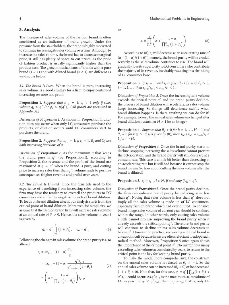
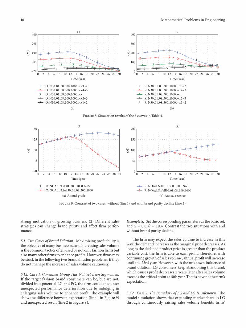
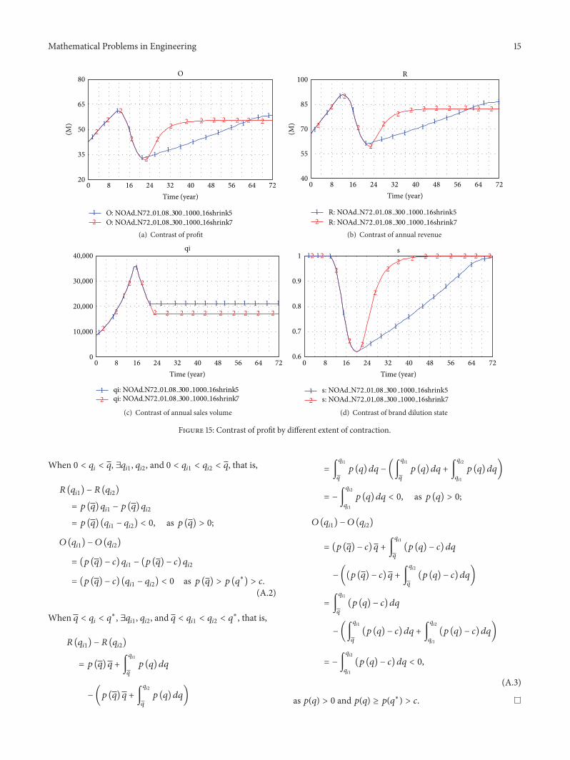its plan of entering the mass market that could dilute LVbrand These phenomena are known as ldquobrand dilutionrdquoreferring to the weakening of a brand due to its overuseBrand dilution frequently happens as a result of unsuccessfulbrand extension [12ndash14]

Price cutting might increase sales volume but might alsodamage brand equity [11] Brand extension which extends theoriginal brand to the newmarkets could exert dilution effectson the parent brand when the attributes of extended brandsare inconsistent with the original brand positioning [1 15ndash17]Many related studies in fashion industry explained why somefactors are critical for brand extension success [18ndash20] Thispaper focuses on expanding the customer base to nontargetconsumers by cutting priceThis brand dilution factor resultsfrom social influences such as conspicuous consumption [23 11 20]

Han et al [21] demonstrate with field experiments andmarket data that a market segmentrsquos preference for con-spicuously (or inconspicuously) branded luxury product issignificantly related with consumersrsquo desire to be associatedor dissociated with the members of that segment Priorstudies have identified two competing social needs amongconsumers a need for uniqueness and a countervailing needfor conformity [22 23] Research in the area of referencegroup suggests the differences between consumer groupsFor example consumers from the elite group would liketo distinguish themselves from the masses in consumptionbut the masses seek to emulate the choices of the elites [2425] Therefore we build the model based on two groups ofconsumers namely the leader-group (LG) consumers andthe follower-group (FG) consumers LG consumers seek forthe uniqueness and devalue a brand owned by too many FGwhereas FG consumers would like to follow LG and makethe purchasing decisions when prices are acceptable [7 26]Assuming that the fashion firm can change sales volume byadjusting product prices we expect that the demand from FGwill be increased when price is lowered A higher demand ofLG induces a higher demand of FG while a higher demandof FG leads to a lower demand of LG

The impact of brand dilution on firm performance iswidely observed and discussed [12 27 28] especially infashion industry [29] Some empirical studies measured theindexes of brand dilution and its moderating effect [13 14 3031] Here we use the concept of brand purity to denote thedegree of brand dilution that is defined in the mathematicmodel

While many cases suggest the essential tradeoff thatfashion brands need to make between increasing marketshare and degrading brand value there is little research thathas analyzed the dynamic mechanism of brand dilutionTherefore we establish a dynamic brand dilution model andinvestigate analytically and numerically the situations wherebrand dilution occurs the effects of brand dilution on brandfirm performance and the strategies to cope with branddilution The findings provide managerial implications forfashion firms regarding how to achieve the balance betweenmarket extension and brand dilution to optimize the firmperformance

119875

119902lowast

IIIIII

119876119902

119875

119902

Figure 1 Demand curve and sales revenue

For the numerical analysis we use the System Dynamics(SD) that is a widely used methodology and mathematicalmodeling technique that clearly visualizes the model Byusing SD model the dynamic brand dilution model is vividand is easier to understand In addition SD model is suitableto conduct stimulation for a particular case and to produceiteration results It also acts as a delicate what-if tool formanagers to conveniently modify specific variables of themodel based on their needs and observe stimulation resultsunder different conditions

This paper contributes to the literature by (1) firstintroducing the idea of the brand purity and proposing aquantitative measure of brand dilution level (2) establishingthe dynamic brand dilution model and (3) demonstratinganalytically and numerically how dynamic changes of salesvolumes affect the brand purity and the firm performance

We develop an economic model for the mechanism ofbrand dilution in Section 2 and analyze the process of howbrand dilution and firm performance develops in Section 3The related system dynamics model and the numerical anal-ysis appear in Section 4 Simulations on luxury fashion brandbackground further validate the process of brand dilution inSection 5 Conclusions are summarized in Section 6

2 Model

21 Price-Sales Volume Relation To simplify the configu-ration we use demand curves to describe the relationshipbetween the selling price and the quantity (sales volume)of a fashion brand in Figure 1 Given the existing productportfolio of the fashion brand let 119901 be the highest price ofthe branded products within the product portfolio and 119902

the corresponding sales volume of these products Within acertain period price will be arbitrarily modified to adapt tothe market thus gradually falling below the starting price 119901Let 119901 = 119901(119902) where 119901 gt 0 119902 gt 0 119889119901119889119902 lt 0 11988921199011198891199022 ge 0 bethe price function The price function indicates that the finalsale volume is 119902 if the final retail price is set at 119901(119902) The firmcan reduce price to boost sales

The revenue of the fashion brand is calculated by accu-mulating the product of the price and the quantity on thedemand curve for example if the final price is 119901(119902) thenthe revenue of all the goods with 100 brand purity (thedefinition of brand purity and its effects on revenue arediscussed later in this section) is given by the sum of areasI II and III in Figure 1







119871be the sales




119871+ 119902

119865


119871(119902

119871+ 119902




119877 = 119901 (119902) 119902119904 + int

119902

119902

119901 (119902) 119904119889119902 for 119902 le 119902lowast (1a)

119877 = 119901 (119902) 119902119904 + int

119902lowast

119902

119901 (119902) 119904119889119902 + int

119902

119902lowast

119901 (119902) 119889119902 for 119902 gt 119902lowast

(1b)






119874 = (119901 (119902) minus 119888) 119902119904 + int

119902

119902


(2a)

119874 = (119901 (119902) minus 119888) 119902119904 + int

119902lowast

119902

(119901 (119902) minus 119888) 119904119889119902 minus 119862

+ int

119902

119902lowast




119894 119877119894 and 119874

119894(we


119904

119894= 120572119904

119894minus1+ (1 minus 120572)

119902

119871119894

119902

119894

119904

0= 1 (3)

where 0 lt 120572 lt 1 119902119871119894







119871119894119902

119894We set 119904

0= 1 and assume





119877

119894= 119901 (119902) 119902119904

119894minus1+ int

119902lowast

119902

119901 (119902) 119904

119894minus1119889119902

+ int

119902119894+(1minus119904


119902lowast

119901 (119902) 119889119902 for 119901119894lt 119901 (119902

lowast)

(4)


119894minus1 As 119902119871119894= 119904

119894minus1119902

lowast

and 119902119865119894= 119902

119894minus119904

119894minus1119902


119894+(1minus119904

119894minus1)119902

lowast) = 119901(119902

lowast+119902

119865119894) to obtain 119902



119874

119894= (119901 (119902) minus 119888) 119902119904

119894minus1+ int

119902lowast

119902

(119901 (119902) minus 119888) 119904

119894minus1119889119902

+ int

119902119894+(1minus119904


119902lowast


lowast)

(5)



3 Analysis




= 1 119904119894lt 1 only if sales

volume 119902119894gt 119902

lowast (or 119901119894le 119901(119902


Appendix A)



= 1 if 119904119894= 1 119877

119894and 119874

119894are







is given by

119902

119894= 119902

lowast

119894

prod

119895=1

(1 + 120579

119895) 119902

0= 119902

lowast (6)


119904

119894= 120572119904

119894minus1+ (1 minus 120572)

119902

119871119894

119902

119894

= 120572119904

119894minus1+ (1 minus 120572)

119902

lowast119904

119894minus1

119902

lowastprod

119894

119895=1(1 + 120579

119895)

= (120572 +

1 minus 120572

prod

119894

119895=1(1 + 120579

119895)

) 119904

119894minus1

(7)

or

119904

119894=

119894

prod

119896=1

(120572 +

1 minus 120572

prod

119896

119895=1(1 + 120579

119895)

) (8)


(120572+ (1minus120572)(1 + 120579)




119894is given by (8) with 120579

119894gt 0

119894 = 1 2 then 119904119894+2119904

119894+1lt 119904

119894+1119904

119894lt 1



120579

119896= 0 for 119896 ge 119867 If 119904

119894is given by (8) then 119904

119894+2119904

119894+1= 119904

119894+1119904

119894lt

1 for 119894 gt 119867


Proposition 5 119904119894ge 119904


119894le 119902

lowast








(minus1 lt 120579


119894= 119902

lowastprod

119894

119895=1(1 + 120579

119895) lt

119902

lowast119904



LG in year 119894 if 119902119894lt 119902

lowast119904

119894minus1 then 119902

119871119894= 119902




119871119894= min119902lowast119904

119894minus1 119902

119894 Moreover 119902

119894le 119902

lowast119904

119894minus1means


119904

119894=

120572119904

119894minus1+ (1 minus 120572)

119902

119871119894

119902

119894

for 119902119894gt 119902

119871119894

120572119904

119894minus1+ (1 minus 120572) for 119902

119894= 119902

119871119894

(9)

If 119902119894gt 119902



119895) gt 119902

lowast119904




119894=

119902


119894lt

(119904

119894minus1prod

119894minus1

119895=1(1 + 120579





120579

119896= 0 for 119896 ge 119867 If 119904

1lt 1 then 119877

119894lt 119877

119894minus1 119874119894lt 119874

119894minus1119874

119894minus

119874





s

aqL

O

k b cc C

R

qi

qlowast

q998400




119894qi

119902


119871119894qL

120572 a119902 q1015840119862 C119888 cc119904

119894s

119877

119894R

119874

119894O




119894is the sales


119895in (6) Variable 119904












119894from (4) is

119877

119894= (119887 minus 119896119902) 119902119904

119894minus1+ (2119887 minus 119896 (119902

lowast+ 119902)) (119902


119894minus1

+ (2119887 minus 119896 (119902

119894+ (1 minus 119904

119894minus1) 119902

lowast+ 119902

lowast))

times ((119902

119894+ (1 minus 119904

119894minus1) 119902

lowast+ 119902

lowast))

(10)


+ (

1

2



)







Line 119887 119896 (119901

lowast 119902

lowast)

1 5000 020 (1000 20000)2 4000 015 (1000 20000)3 3000 010 (1000 20000)4 2600 008 (1000 20000)5 2000 005 (1000 20000)6 1400 002 (1000 20000)7 1200 001 (1000 20000)









1

1

1

1

1

2

2

2

2

2

3

33

3

3

4

44

4

4

5

55

5

5

6

66

6 6

7

77

77 7

7

60

45

30

15

00

2 4 6 8 10 12 14 16 18 20 22 24 26 28 30

O

Time (year)

(M)

O N30 01 08 300 1000 02O N30 01 08 300 1000 015O N30 01 08 300 1000 01O N30 01 08 300 1000 008O N30 01 08 300 1000 005O N30 01 08 300 1000 002O N30 01 08 300 1000 001

(a)

7

1

1

1

1

1

2

2

2

2

2

3

33

3

3

4

44

4

4

5

55 5

5

6

66

66

7

77

77 7

R80

60

40

20

00 2 4 6 8 10 12 14 16 18 20 22 24 26 28 30

Time (year)

(M)

R N30 01 08 300 1000 02R N30 01 08 300 1000 015R N30 01 08 300 1000 01R N30 01 08 300 1000 008R N30 01 08 300 1000 005R N30 01 08 300 1000 002R N30 01 08 300 1000 001

(b)


1

1

1

1

1

2

2

2

2

3

3

33

4

44

4

5

55

5

6

66

66

7

77

7 7

60

45

30

15

00

2 4 6 8 10 12 14 16 18 20 22 24 26 28 30

O

Time (year)

7

(M)

O N30 01 05 300 1000 02O N30 01 05 300 1000 015O N30 01 05 300 1000 01O N30 01 05 300 1000 008O N30 01 05 300 1000 005O N30 01 05 300 1000 002O N30 01 05 300 1000 001

(a)

0

1

1

1

1

1

2

2

2

2

3

33

3

4

44

4

5

55

5

6

66

6 6

7

77

77

7 7

R80

60

40

20

0 2 4 6 8 10 12 14 16 18 20 22 24 26 28 30Time (year)

R N30 01 05 300 1000 02R N30 01 05 300 1000 015R N30 01 05 300 1000 01R N30 01 05 300 1000 008R N30 01 05 300 1000 005R N30 01 05 300 1000 002R N30 01 05 300 1000 001

(M)

(b)





119902lowast

119875

119902

(a)

119902lowast

119875

119902

(b)


8

3

12

2

22

2

2

3

33

3

3

4

4

4

44

5

5

5

5

6

6

6

6

7

77

7

7

8

88 8

8

0 2 4 6 8 10 12 14 16 18 20 22 24 26 28 30Time (year)

60

30

0

minus30

minus60

O

11

1

1

576

(M)


(a)

8

1

1

11

1

2

2

2

3

3

3

4

4

4 4 44

5

55

5

6

66

6

7

77

77

8

88 8

8

0 2 4 6 8 10 12 14 16 18 20 22 24 26 28 30Time (year)

80

55

30

5

minus20

R

2

2

23

3

3

6 5


(M)

(b)











Fold Line Line 119887 119896 (119901

lowast 119902

lowast) Line 119887 119896

1 1 5000 020 (1000 20000) 4 2600 0082 1 5000 020 (1000 20000) 5 2000 0053 1 5000 020 (1000 20000) 6 1400 0024 1 5000 020 (1000 20000) 7 1200 0015 3 3000 010 (1000 20000) 4 2600 0086 3 3000 010 (1000 20000) 5 2000 0057 3 3000 010 (1000 20000) 6 1400 0028 3 3000 010 (1000 20000) 7 1200 001


Curve 119887 119896 (119901

lowast 119902

lowast)

1 32 2828430000 (1000 20000)2 43 542884000 (1000 20000)3 1 20000000 (1000 20000)4 23 736806 (1000 20000)5 12 141421 (1000 20000)

4000

3000

2000

1000

00 5000 10000 15000 20000 25000 30000 35000 40000

119901 = 2828430000119902(32)

119901 = 542884000119902(43)

119901 = 20000000119902

119901 = 736806119902(23)

119901 = 141421119902(12)













3

400

295

190

85

minus200 2 4 6 8 10 12 14 16 18 20 22 24 26 28 30

Time (year)

O

2

2 2 2 2 22

22

2

3

3 3 3 3 3 3 3 3

4

4 4 4 4 4 4 4

1

1 1 1 11

11

11

5

5 5 5 5 5 5 5 5

(M)


4

(a)

4 3

400

00 2

2

2 2 2 2 22

2 2 2

3

3 3 3 3 3 3 3 3

4

4 4 4 4 4 4 4

1

1 1 1 11

11

11

5

5 5 5 5 5 5 5 5

4 6 8 10 12 14 16 18 20 22 24 26 28 30

300

200

100

Time (year)

R

(M)


(b)


2 2

O80

55

30

5

minus200 2 4 6 8 10 12 14 16 18 20 22 24 26 28 30

Time (year)

1

1 1 1 1 1 1 1 1 11 1 1 1 1 1

2

222

22

2

22

22

22

(M)


(a) Annual profit

2 2

R200

150

100

50

0

1

1 1 1 1 1 1 1 1 1 1 1 1 1 1

1

2

2 2 2 2 2 2 2 2 2 2 2 2

02 4 6 8 10 12 14 16 18 20 22 24 26 28 30

Time (year)


(M)

(b) Annual revenue









60

55

50

45

400 2 4 6 8 10 12 14 16 18 20 22 24 26 28 30

Time (year)

O

2

2

2 2 2 2 2 2 2 2 2 2 2 2

2

3

3 3 3 3 3 3 3 3 3 3 3 3 3 3

1

1

1

1

1

11 1 1 1 1 1 1 111

(M)


(a) Annual profit


40000

30000

20000

10000

qi

002 4 6 8 10 12 14 16 18 20 22 24 26 28 30

Time (year)

2

2 2 2 2 2 2 2 2 2 2222

2

3

3 3 3 3 3 3 3 3333333

1

11

11

1 1 1 1 1 1 1 1 1 1 1



4

3

33 32

80

55

30

5

minus20

O

0 2 4 6 8 10 12 14 16 18 20 22 24 26 28 30

Time (year)

2

22

2

2 22

22

22

3

3

33

3 3

4

44

4

44

44

44

1

1 111

1 1 1 1 1 11

33

(M)


(a) Annual profit

4 4

44


200000

150000

100000

50000

qi

002 4 6 8 10 12 14 16 18 20 22 24 26 28 30

Time (year)

2

2 2 2 2 2 2 2 22 22

3

3 3 3 33 3

3 3 3

3

1

1 1

4

44

4

4

4 41 1 1 1 1 1 1 11











O80

55

30

5

minus200 2 4 6 8 10 12 14 16 18 20 22 24 26 28 30

Time (year)

1

1 1 1 1 1 1 11

11

11

1

11

(M)

O NOAd N full30 01 08 300 1000

(a) Profit

R100

85

70

55

400 2 4 6 8 10 12 14 16 18 20 22 24 26 28 30

Time (year)

1

11

11

11 1

1

1

11

11 1 1

(M)

R NOAd N full30 01 08 300 1000

(b) Revenue

1

1 1 1 1 1 1 1 1 11

11

11

qi200000

150000

100000

50000

00

2 4 6 8 10 12 14 16 18 20 22 24 26 28 30Time (year)

qi NOAd N full30 01 08 300 1000

(c) Sales volume

1

1 1 1 1 1 11

1

11

11

1 1 1

s1

075

05

025

00

2 4 6 8 10 12 14 16 18 20 22 24 26 28 30Time (year)

s NOAd N full30 01 08 300 1000

(d) Brand purity



119894= 119902

lowast(1 + 120579)










O80

55

30

5

minus200 2 4 6 8 10 12 14 16 18 20 22 24 26 28 30

Time (year)

21

2 2 2 2 2 2 2

2222

222

1111

1 1 1 1

11

11

11

1

1

(M)



R

0

Time (year)

2

2 2 2 2 22

2222

22

22

1

1 1 1 1 1 1 1 11

11 1 1 1 1

100

75

50

25

0 2 4 6 8 10 12 14 16 18 20 22 24 26 28 30


(M)


qi200000

150000

100000

50000

002 4 6 8 10 12 14 16 18 20 22 24 26 28 30

Time (year)

2

2 2 2 22 2 22222

221 1 1

1

1 1 1 1 1 1 11

11

1



s1

075

05

025

0

Time (year)

21

2 2 2 2 22

2

22

22

22 2 2

1 1 1 1 1 11

1

1

1

11

1 11

0 2 4 6 8 10 12 14 16 18 20 22 24 26 28 30












80

60

40

20

O

005 10 15 20 25 30 35 40 45 50

Time (year)

1

1

1 11

1

1 1 1 1 1 11

1

1

1

2

22

2 2

2

22 2 2

2 2 2 2

2

3

33

3 3

33

3 3 3

33 3

33

(M)


(a) Annual profit


1

075

05

025

s

005 10 15 20 25 30 35 40 45 50

Time (year)

1

1 11

1

1

11

1 1 1 1 11

1 1

2

2 2 22

2

2

2

22

2 2 22 22

3

3 3 33

3

3

33

3 3 3 3 3 3






6 Conclusion




Appendices



119894le 119902


119871119894gt


119894= 1


119894le 119902


119894le 119902

lowast

119877

119894= 119901 (119902) 119902119904

119894minus1+ int

119902119894

119902

119901 (119902) 119904

119894minus1119889119902

119874

119894= (119901 (119902) minus 119888) 119902119904

119894minus1+ int

119902119894

119902

(119901 (119902) minus 119888) 119904

119894minus1119889119902

(A1)


O80

65

50

35

200 8

1

1

1

1

1

1 1 1 1 1 1

1 1111

2

22

2

2

2

2

2 2 2 22222

16 24 32 40 48 56 64 72Time (year)

(M)



R100

85

70

55

400 8 16 24 32 40 48 56 64 72

Time (year)

1

1

1

1

1

1 1 1 11

1 1

1 111

2

2

22

2

2

22 2 2 2 2 2 2 2

(M)



1

1

1

1

1

1 1 1 1 1 1 1 1 11111

2

2

2

22

2 2 2 2222222

qi40000

30000

20000

10000

00

8 16 24 32 40 48 56 64 72Time (year)



1

1 1 1

1

11

11

11

11

11

2

2 2

2

2 2

2

22 2 2 2 2222s

1

09

08

07

060 8 16 24 32 40 48 56 64 72

Time (year)




When 0 lt 119902119894lt 119902 exist119902

1198941 1199021198942 and 0 lt 119902

1198941lt 119902

1198942lt 119902 that is

119877 (119902

1198941) minus 119877 (119902

1198942)

= 119901 (119902) 119902

1198941minus 119901 (119902) 119902

1198942

= 119901 (119902) (119902

1198941minus 119902

1198942) lt 0 as 119901 (119902) gt 0

119874 (119902

1198941) minus 119874 (119902

1198942)

= (119901 (119902) minus 119888) 119902

1198941minus (119901 (119902) minus 119888) 119902

1198942

= (119901 (119902) minus 119888) (119902

1198941minus 119902

1198942) lt 0 as 119901 (119902) gt 119901 (119902lowast) gt 119888

(A2)

When 119902 lt 119902119894lt 119902


1198941lt 119902

1198942lt 119902

lowast that is

119877 (119902

1198941) minus 119877 (119902

1198942)

= 119901 (119902) 119902 + int

1199021198941

119902

119901 (119902) 119889119902

minus (119901 (119902) 119902 + int

1199021198942

119902

119901 (119902) 119889119902)

= int

1199021198941

119902

119901 (119902) 119889119902 minus (int

1199021198941

119902

119901 (119902) 119889119902 + int

1199021198942

1199021198941

119901 (119902) 119889119902)

= minusint

1199021198942

1199021198941

119901 (119902) 119889119902 lt 0 as 119901 (119902) gt 0

119874 (119902

1198941) minus 119874 (119902

1198942)

= (119901 (119902) minus 119888) 119902 + int

1199021198941

119902

(119901 (119902) minus 119888) 119889119902

minus ((119901 (119902) minus 119888) 119902 + int

1199021198942

119902

(119901 (119902) minus 119888) 119889119902)

= int

1199021198941

119902

(119901 (119902) minus 119888) 119889119902

minus (int

1199021198941

119902

(119901 (119902) minus 119888) 119889119902 + int

1199021198942

1199021198941

(119901 (119902) minus 119888) 119889119902)

= minusint

1199021198942

1199021198941

(119901 (119902) minus 119888) 119889119902 lt 0

(A3)




119894

119896=1(120572 + (1 minus 120572)

(prod

119896

119895=1(1 + 120579

119895))) when 119902

0= 119902


119904

1= 120572 +

1 minus 120572

1 + 120579

1

lt 120572 +

1 minus 120572

1

= 1 as 1205791gt 0

119904

119894+2

119904

119894+1

= (120572 +

1 minus 120572

prod

119894+2

119895=1(1 + 120579

119895)

)

119904

119894+1

119904

119894

= (120572 +

1 minus 120572

prod

119894+1

119895=1(1 + 120579

119895)

)

(A4)


119894+2

prod

119895=1

(1 + 120579

119895) gt

119894+1

prod

119895=1

(1 + 120579

119895) gt 1 (A5)

that is

(120572 +

1 minus 120572

prod

119894+2

119895=1(1 + 120579

119895)

) lt (120572 +

1 minus 120572

prod

119894+1

119895=1(1 + 120579

119895)

)

lt (120572 +

1 minus 120572

1

) = 1

119904

119894

119904

119894minus1

lt

119904

119894minus1

119904

119894minus2

lt 1

(A6)


119904

119894+2

119904

119894+1

= (120572 +

1 minus 120572

prod

119894+2

119896=1(1 + 120579

119896)

)

= (120572 +

1 minus 120572

prod

119867minus1

119896=1(1 + 120579

119896)prod

119894+2

119896=119867(1 + 120579

119896)

)

as 120579119896= 0 when 119896 ge 119867 120579

119896gt 0

(A7)


119904

119894+2

119904

119894+1

= (120572 +

1 minus 120572

prod

119867minus1

119896=1(1 + 120579

119896)

) lt 1 (A8)

Similarly

119904

119894+1

119904

119894

= (120572 +

1 minus 120572

prod

119867minus1

119896=1(1 + 120579

119896)

) lt 1

119904

119894+2

119904

119894+1

=

119904

119894+1

119904

119894

lt 1

(A9)


lowast119904

119894minus1 then 119902

119871119894= 119902

119894 By (3)

119904

119894gt 119904

119894minus1 If 119902lowast119904

119894minus1le 119902

119894 then 119902

119871119894= 119902

lowast119904

119894minus1 By (3) 119904

119894= 120572119904

119894minus1+

(1minus120572)(119902

119871119894119902

119894) = 120572119904

119894minus1+(1minus120572)(119902

lowast119904

119894minus1119902

119894) and 119904

119894gt 120572119904


120572)(119902

lowast119904

119894minus1119902

lowast) = 119904

119894minus1 If 119904119894ge 119904

119894minus1 120572119904119894minus1

+ (1 minus 120572)(119902

lowast119904

119894minus1119902

119894) ge

119904

119894minus1 then 119902

119894lt 119902

lowast


119877

119894minus 119877

119894minus1

= 119901 (119902) 119902 (119904


119894minus2)

+ int

119902lowast

119902

119901 (119902) 119889119902 (119904


119894minus2)

+ int

119902119894+(1minus119904



119901 (119902) 119889119902

119877

119894minus 119877

119894minus1

= (119901 (119902) 119902 + int

119902lowast

119902

119901 (119902) 119889119902)

times (119904


119894minus2) + int

119902119894+(1minus119904



119901 (119902) 119889119902

lt (119901 (119902) 119902 + int

119902lowast

119902

119901 (119902) 119889119902) (119904


119894minus2)

minus 119901 (119902

119894+ (1 minus 119904

119894minus2) 119902

lowast) 119902

lowast(119904


119894minus2)

119877

119894minus 119877

119894minus1

lt (119901 (119902) 119902 + int

119902lowast

119902

119901 (119902) 119889119902 minus 119901 (119902

119894+ (1 minus 119904

119894minus1) 119902

lowast) 119902

lowast)

times (119904


119894minus2)

lt (119901 (119902

lowast) 119902


119894+ (1 minus 119904

119894minus2) 119902

lowast) 119902

lowast)

times (119904


119894minus2)

(A10)


(119901 (119902

lowast) 119902


119894+ (1 minus 119904

119894minus2) 119902

lowast) 119902

lowast) gt 0 (A11)


119894+ (1 minus 119904

119894minus2)119902


0= 1

119904

1lt 1 then 119902

1gt 119902

lowast 1199022ge 119902

1 so 119902lowast lt 119902

119894when 119894 ge 2 and

119904



119894minus2lt 0 So 119877

119894minus 119877

119894minus1lt 0

Similarly

119874

119894minus 119874

119894minus1= (119901 (119902) minus 119888) 119902 (119904


119894minus2)

+ int

119902lowast

119902

(119901 (119902) minus 119888) 119889119902 (119904


119894minus2)

+ int

119902119894+(1minus119904



(119901 (119902) minus 119888) 119889119902

= 119901 (119902) 119902 (119904


119894minus2)

+ int

119902lowast

119902

119901 (119902) 119889119902 (119904


119894minus2)

+ int

119902119894+(1minus119904



119901 (119902) 119889119902

= 119877

119894minus 119877

119894minus1lt 0

(A12)




(01) a = 08(02) b = 1400(03) C = 100000

(04) cc = 300(05) FINAL TIME = 30









(01) a = 08(02) C = 20000000







Acknowledgments


References









































Volume 2014




Journal of











Journal of


Function Spaces






Algebra















119871be the sales




119871+ 119902

119865


119871(119902

119871+ 119902




119877 = 119901 (119902) 119902119904 + int

119902

119902

119901 (119902) 119904119889119902 for 119902 le 119902lowast (1a)

119877 = 119901 (119902) 119902119904 + int

119902lowast

119902

119901 (119902) 119904119889119902 + int

119902

119902lowast

119901 (119902) 119889119902 for 119902 gt 119902lowast

(1b)






119874 = (119901 (119902) minus 119888) 119902119904 + int

119902

119902


(2a)

119874 = (119901 (119902) minus 119888) 119902119904 + int

119902lowast

119902

(119901 (119902) minus 119888) 119904119889119902 minus 119862

+ int

119902

119902lowast




119894 119877119894 and 119874

119894(we


119904

119894= 120572119904

119894minus1+ (1 minus 120572)

119902

119871119894

119902

119894

119904

0= 1 (3)

where 0 lt 120572 lt 1 119902119871119894







119871119894119902

119894We set 119904

0= 1 and assume





119877

119894= 119901 (119902) 119902119904

119894minus1+ int

119902lowast

119902

119901 (119902) 119904

119894minus1119889119902

+ int

119902119894+(1minus119904


119902lowast

119901 (119902) 119889119902 for 119901119894lt 119901 (119902

lowast)

(4)


119894minus1 As 119902119871119894= 119904

119894minus1119902

lowast

and 119902119865119894= 119902

119894minus119904

119894minus1119902


119894+(1minus119904

119894minus1)119902

lowast) = 119901(119902

lowast+119902

119865119894) to obtain 119902



119874

119894= (119901 (119902) minus 119888) 119902119904

119894minus1+ int

119902lowast

119902

(119901 (119902) minus 119888) 119904

119894minus1119889119902

+ int

119902119894+(1minus119904


119902lowast


lowast)

(5)



3 Analysis




= 1 119904119894lt 1 only if sales

volume 119902119894gt 119902

lowast (or 119901119894le 119901(119902


Appendix A)



= 1 if 119904119894= 1 119877

119894and 119874

119894are







is given by

119902

119894= 119902

lowast

119894

prod

119895=1

(1 + 120579

119895) 119902

0= 119902

lowast (6)


119904

119894= 120572119904

119894minus1+ (1 minus 120572)

119902

119871119894

119902

119894

= 120572119904

119894minus1+ (1 minus 120572)

119902

lowast119904

119894minus1

119902

lowastprod

119894

119895=1(1 + 120579

119895)

= (120572 +

1 minus 120572

prod

119894

119895=1(1 + 120579

119895)

) 119904

119894minus1

(7)

or

119904

119894=

119894

prod

119896=1

(120572 +

1 minus 120572

prod

119896

119895=1(1 + 120579

119895)

) (8)


(120572+ (1minus120572)(1 + 120579)




119894is given by (8) with 120579

119894gt 0

119894 = 1 2 then 119904119894+2119904

119894+1lt 119904

119894+1119904

119894lt 1



120579

119896= 0 for 119896 ge 119867 If 119904

119894is given by (8) then 119904

119894+2119904

119894+1= 119904

119894+1119904

119894lt

1 for 119894 gt 119867


Proposition 5 119904119894ge 119904


119894le 119902

lowast








(minus1 lt 120579


119894= 119902

lowastprod

119894

119895=1(1 + 120579

119895) lt

119902

lowast119904



LG in year 119894 if 119902119894lt 119902

lowast119904

119894minus1 then 119902

119871119894= 119902




119871119894= min119902lowast119904

119894minus1 119902

119894 Moreover 119902

119894le 119902

lowast119904

119894minus1means


119904

119894=

120572119904

119894minus1+ (1 minus 120572)

119902

119871119894

119902

119894

for 119902119894gt 119902

119871119894

120572119904

119894minus1+ (1 minus 120572) for 119902

119894= 119902

119871119894

(9)

If 119902119894gt 119902



119895) gt 119902

lowast119904




119894=

119902


119894lt

(119904

119894minus1prod

119894minus1

119895=1(1 + 120579





120579

119896= 0 for 119896 ge 119867 If 119904

1lt 1 then 119877

119894lt 119877

119894minus1 119874119894lt 119874

119894minus1119874

119894minus

119874





s

aqL

O

k b cc C

R

qi

qlowast

q998400




119894qi

119902


119871119894qL

120572 a119902 q1015840119862 C119888 cc119904

119894s

119877

119894R

119874

119894O




119894is the sales


119895in (6) Variable 119904












119894from (4) is

119877

119894= (119887 minus 119896119902) 119902119904

119894minus1+ (2119887 minus 119896 (119902

lowast+ 119902)) (119902


119894minus1

+ (2119887 minus 119896 (119902

119894+ (1 minus 119904

119894minus1) 119902

lowast+ 119902

lowast))

times ((119902

119894+ (1 minus 119904

119894minus1) 119902

lowast+ 119902

lowast))

(10)


+ (

1

2



)







Line 119887 119896 (119901

lowast 119902

lowast)

1 5000 020 (1000 20000)2 4000 015 (1000 20000)3 3000 010 (1000 20000)4 2600 008 (1000 20000)5 2000 005 (1000 20000)6 1400 002 (1000 20000)7 1200 001 (1000 20000)









1

1

1

1

1

2

2

2

2

2

3

33

3

3

4

44

4

4

5

55

5

5

6

66

6 6

7

77

77 7

7

60

45

30

15

00

2 4 6 8 10 12 14 16 18 20 22 24 26 28 30

O

Time (year)

(M)

O N30 01 08 300 1000 02O N30 01 08 300 1000 015O N30 01 08 300 1000 01O N30 01 08 300 1000 008O N30 01 08 300 1000 005O N30 01 08 300 1000 002O N30 01 08 300 1000 001

(a)

7

1

1

1

1

1

2

2

2

2

2

3

33

3

3

4

44

4

4

5

55 5

5

6

66

66

7

77

77 7

R80

60

40

20

00 2 4 6 8 10 12 14 16 18 20 22 24 26 28 30

Time (year)

(M)

R N30 01 08 300 1000 02R N30 01 08 300 1000 015R N30 01 08 300 1000 01R N30 01 08 300 1000 008R N30 01 08 300 1000 005R N30 01 08 300 1000 002R N30 01 08 300 1000 001

(b)


1

1

1

1

1

2

2

2

2

3

3

33

4

44

4

5

55

5

6

66

66

7

77

7 7

60

45

30

15

00

2 4 6 8 10 12 14 16 18 20 22 24 26 28 30

O

Time (year)

7

(M)

O N30 01 05 300 1000 02O N30 01 05 300 1000 015O N30 01 05 300 1000 01O N30 01 05 300 1000 008O N30 01 05 300 1000 005O N30 01 05 300 1000 002O N30 01 05 300 1000 001

(a)

0

1

1

1

1

1

2

2

2

2

3

33

3

4

44

4

5

55

5

6

66

6 6

7

77

77

7 7

R80

60

40

20

0 2 4 6 8 10 12 14 16 18 20 22 24 26 28 30Time (year)

R N30 01 05 300 1000 02R N30 01 05 300 1000 015R N30 01 05 300 1000 01R N30 01 05 300 1000 008R N30 01 05 300 1000 005R N30 01 05 300 1000 002R N30 01 05 300 1000 001

(M)

(b)





119902lowast

119875

119902

(a)

119902lowast

119875

119902

(b)


8

3

12

2

22

2

2

3

33

3

3

4

4

4

44

5

5

5

5

6

6

6

6

7

77

7

7

8

88 8

8

0 2 4 6 8 10 12 14 16 18 20 22 24 26 28 30Time (year)

60

30

0

minus30

minus60

O

11

1

1

576

(M)


(a)

8

1

1

11

1

2

2

2

3

3

3

4

4

4 4 44

5

55

5

6

66

6

7

77

77

8

88 8

8

0 2 4 6 8 10 12 14 16 18 20 22 24 26 28 30Time (year)

80

55

30

5

minus20

R

2

2

23

3

3

6 5


(M)

(b)











Fold Line Line 119887 119896 (119901

lowast 119902

lowast) Line 119887 119896

1 1 5000 020 (1000 20000) 4 2600 0082 1 5000 020 (1000 20000) 5 2000 0053 1 5000 020 (1000 20000) 6 1400 0024 1 5000 020 (1000 20000) 7 1200 0015 3 3000 010 (1000 20000) 4 2600 0086 3 3000 010 (1000 20000) 5 2000 0057 3 3000 010 (1000 20000) 6 1400 0028 3 3000 010 (1000 20000) 7 1200 001


Curve 119887 119896 (119901

lowast 119902

lowast)

1 32 2828430000 (1000 20000)2 43 542884000 (1000 20000)3 1 20000000 (1000 20000)4 23 736806 (1000 20000)5 12 141421 (1000 20000)

4000

3000

2000

1000

00 5000 10000 15000 20000 25000 30000 35000 40000

119901 = 2828430000119902(32)

119901 = 542884000119902(43)

119901 = 20000000119902

119901 = 736806119902(23)

119901 = 141421119902(12)













3

400

295

190

85

minus200 2 4 6 8 10 12 14 16 18 20 22 24 26 28 30

Time (year)

O

2

2 2 2 2 22

22

2

3

3 3 3 3 3 3 3 3

4

4 4 4 4 4 4 4

1

1 1 1 11

11

11

5

5 5 5 5 5 5 5 5

(M)


4

(a)

4 3

400

00 2

2

2 2 2 2 22

2 2 2

3

3 3 3 3 3 3 3 3

4

4 4 4 4 4 4 4

1

1 1 1 11

11

11

5

5 5 5 5 5 5 5 5

4 6 8 10 12 14 16 18 20 22 24 26 28 30

300

200

100

Time (year)

R

(M)


(b)


2 2

O80

55

30

5

minus200 2 4 6 8 10 12 14 16 18 20 22 24 26 28 30

Time (year)

1

1 1 1 1 1 1 1 1 11 1 1 1 1 1

2

222

22

2

22

22

22

(M)


(a) Annual profit

2 2

R200

150

100

50

0

1

1 1 1 1 1 1 1 1 1 1 1 1 1 1

1

2

2 2 2 2 2 2 2 2 2 2 2 2

02 4 6 8 10 12 14 16 18 20 22 24 26 28 30

Time (year)


(M)

(b) Annual revenue









60

55

50

45

400 2 4 6 8 10 12 14 16 18 20 22 24 26 28 30

Time (year)

O

2

2

2 2 2 2 2 2 2 2 2 2 2 2

2

3

3 3 3 3 3 3 3 3 3 3 3 3 3 3

1

1

1

1

1

11 1 1 1 1 1 1 111

(M)


(a) Annual profit


40000

30000

20000

10000

qi

002 4 6 8 10 12 14 16 18 20 22 24 26 28 30

Time (year)

2

2 2 2 2 2 2 2 2 2 2222

2

3

3 3 3 3 3 3 3 3333333

1

11

11

1 1 1 1 1 1 1 1 1 1 1



4

3

33 32

80

55

30

5

minus20

O

0 2 4 6 8 10 12 14 16 18 20 22 24 26 28 30

Time (year)

2

22

2

2 22

22

22

3

3

33

3 3

4

44

4

44

44

44

1

1 111

1 1 1 1 1 11

33

(M)


(a) Annual profit

4 4

44


200000

150000

100000

50000

qi

002 4 6 8 10 12 14 16 18 20 22 24 26 28 30

Time (year)

2

2 2 2 2 2 2 2 22 22

3

3 3 3 33 3

3 3 3

3

1

1 1

4

44

4

4

4 41 1 1 1 1 1 1 11











O80

55

30

5

minus200 2 4 6 8 10 12 14 16 18 20 22 24 26 28 30

Time (year)

1

1 1 1 1 1 1 11

11

11

1

11

(M)

O NOAd N full30 01 08 300 1000

(a) Profit

R100

85

70

55

400 2 4 6 8 10 12 14 16 18 20 22 24 26 28 30

Time (year)

1

11

11

11 1

1

1

11

11 1 1

(M)

R NOAd N full30 01 08 300 1000

(b) Revenue

1

1 1 1 1 1 1 1 1 11

11

11

qi200000

150000

100000

50000

00

2 4 6 8 10 12 14 16 18 20 22 24 26 28 30Time (year)

qi NOAd N full30 01 08 300 1000

(c) Sales volume

1

1 1 1 1 1 11

1

11

11

1 1 1

s1

075

05

025

00

2 4 6 8 10 12 14 16 18 20 22 24 26 28 30Time (year)

s NOAd N full30 01 08 300 1000

(d) Brand purity



119894= 119902

lowast(1 + 120579)










O80

55

30

5

minus200 2 4 6 8 10 12 14 16 18 20 22 24 26 28 30

Time (year)

21

2 2 2 2 2 2 2

2222

222

1111

1 1 1 1

11

11

11

1

1

(M)



R

0

Time (year)

2

2 2 2 2 22

2222

22

22

1

1 1 1 1 1 1 1 11

11 1 1 1 1

100

75

50

25

0 2 4 6 8 10 12 14 16 18 20 22 24 26 28 30


(M)


qi200000

150000

100000

50000

002 4 6 8 10 12 14 16 18 20 22 24 26 28 30

Time (year)

2

2 2 2 22 2 22222

221 1 1

1

1 1 1 1 1 1 11

11

1



s1

075

05

025

0

Time (year)

21

2 2 2 2 22

2

22

22

22 2 2

1 1 1 1 1 11

1

1

1

11

1 11

0 2 4 6 8 10 12 14 16 18 20 22 24 26 28 30












80

60

40

20

O

005 10 15 20 25 30 35 40 45 50

Time (year)

1

1

1 11

1

1 1 1 1 1 11

1

1

1

2

22

2 2

2

22 2 2

2 2 2 2

2

3

33

3 3

33

3 3 3

33 3

33

(M)


(a) Annual profit


1

075

05

025

s

005 10 15 20 25 30 35 40 45 50

Time (year)

1

1 11

1

1

11

1 1 1 1 11

1 1

2

2 2 22

2

2

2

22

2 2 22 22

3

3 3 33

3

3

33

3 3 3 3 3 3






6 Conclusion




Appendices



119894le 119902


119871119894gt


119894= 1


119894le 119902


119894le 119902

lowast

119877

119894= 119901 (119902) 119902119904

119894minus1+ int

119902119894

119902

119901 (119902) 119904

119894minus1119889119902

119874

119894= (119901 (119902) minus 119888) 119902119904

119894minus1+ int

119902119894

119902

(119901 (119902) minus 119888) 119904

119894minus1119889119902

(A1)


O80

65

50

35

200 8

1

1

1

1

1

1 1 1 1 1 1

1 1111

2

22

2

2

2

2

2 2 2 22222

16 24 32 40 48 56 64 72Time (year)

(M)



R100

85

70

55

400 8 16 24 32 40 48 56 64 72

Time (year)

1

1

1

1

1

1 1 1 11

1 1

1 111

2

2

22

2

2

22 2 2 2 2 2 2 2

(M)



1

1

1

1

1

1 1 1 1 1 1 1 1 11111

2

2

2

22

2 2 2 2222222

qi40000

30000

20000

10000

00

8 16 24 32 40 48 56 64 72Time (year)



1

1 1 1

1

11

11

11

11

11

2

2 2

2

2 2

2

22 2 2 2 2222s

1

09

08

07

060 8 16 24 32 40 48 56 64 72

Time (year)




When 0 lt 119902119894lt 119902 exist119902

1198941 1199021198942 and 0 lt 119902

1198941lt 119902

1198942lt 119902 that is

119877 (119902

1198941) minus 119877 (119902

1198942)

= 119901 (119902) 119902

1198941minus 119901 (119902) 119902

1198942

= 119901 (119902) (119902

1198941minus 119902

1198942) lt 0 as 119901 (119902) gt 0

119874 (119902

1198941) minus 119874 (119902

1198942)

= (119901 (119902) minus 119888) 119902

1198941minus (119901 (119902) minus 119888) 119902

1198942

= (119901 (119902) minus 119888) (119902

1198941minus 119902

1198942) lt 0 as 119901 (119902) gt 119901 (119902lowast) gt 119888

(A2)

When 119902 lt 119902119894lt 119902


1198941lt 119902

1198942lt 119902

lowast that is

119877 (119902

1198941) minus 119877 (119902

1198942)

= 119901 (119902) 119902 + int

1199021198941

119902

119901 (119902) 119889119902

minus (119901 (119902) 119902 + int

1199021198942

119902

119901 (119902) 119889119902)

= int

1199021198941

119902

119901 (119902) 119889119902 minus (int

1199021198941

119902

119901 (119902) 119889119902 + int

1199021198942

1199021198941

119901 (119902) 119889119902)

= minusint

1199021198942

1199021198941

119901 (119902) 119889119902 lt 0 as 119901 (119902) gt 0

119874 (119902

1198941) minus 119874 (119902

1198942)

= (119901 (119902) minus 119888) 119902 + int

1199021198941

119902

(119901 (119902) minus 119888) 119889119902

minus ((119901 (119902) minus 119888) 119902 + int

1199021198942

119902

(119901 (119902) minus 119888) 119889119902)

= int

1199021198941

119902

(119901 (119902) minus 119888) 119889119902

minus (int

1199021198941

119902

(119901 (119902) minus 119888) 119889119902 + int

1199021198942

1199021198941

(119901 (119902) minus 119888) 119889119902)

= minusint

1199021198942

1199021198941

(119901 (119902) minus 119888) 119889119902 lt 0

(A3)




119894

119896=1(120572 + (1 minus 120572)

(prod

119896

119895=1(1 + 120579

119895))) when 119902

0= 119902


119904

1= 120572 +

1 minus 120572

1 + 120579

1

lt 120572 +

1 minus 120572

1

= 1 as 1205791gt 0

119904

119894+2

119904

119894+1

= (120572 +

1 minus 120572

prod

119894+2

119895=1(1 + 120579

119895)

)

119904

119894+1

119904

119894

= (120572 +

1 minus 120572

prod

119894+1

119895=1(1 + 120579

119895)

)

(A4)


119894+2

prod

119895=1

(1 + 120579

119895) gt

119894+1

prod

119895=1

(1 + 120579

119895) gt 1 (A5)

that is

(120572 +

1 minus 120572

prod

119894+2

119895=1(1 + 120579

119895)

) lt (120572 +

1 minus 120572

prod

119894+1

119895=1(1 + 120579

119895)

)

lt (120572 +

1 minus 120572

1

) = 1

119904

119894

119904

119894minus1

lt

119904

119894minus1

119904

119894minus2

lt 1

(A6)


119904

119894+2

119904

119894+1

= (120572 +

1 minus 120572

prod

119894+2

119896=1(1 + 120579

119896)

)

= (120572 +

1 minus 120572

prod

119867minus1

119896=1(1 + 120579

119896)prod

119894+2

119896=119867(1 + 120579

119896)

)

as 120579119896= 0 when 119896 ge 119867 120579

119896gt 0

(A7)


119904

119894+2

119904

119894+1

= (120572 +

1 minus 120572

prod

119867minus1

119896=1(1 + 120579

119896)

) lt 1 (A8)

Similarly

119904

119894+1

119904

119894

= (120572 +

1 minus 120572

prod

119867minus1

119896=1(1 + 120579

119896)

) lt 1

119904

119894+2

119904

119894+1

=

119904

119894+1

119904

119894

lt 1

(A9)


lowast119904

119894minus1 then 119902

119871119894= 119902

119894 By (3)

119904

119894gt 119904

119894minus1 If 119902lowast119904

119894minus1le 119902

119894 then 119902

119871119894= 119902

lowast119904

119894minus1 By (3) 119904

119894= 120572119904

119894minus1+

(1minus120572)(119902

119871119894119902

119894) = 120572119904

119894minus1+(1minus120572)(119902

lowast119904

119894minus1119902

119894) and 119904

119894gt 120572119904


120572)(119902

lowast119904

119894minus1119902

lowast) = 119904

119894minus1 If 119904119894ge 119904

119894minus1 120572119904119894minus1

+ (1 minus 120572)(119902

lowast119904

119894minus1119902

119894) ge

119904

119894minus1 then 119902

119894lt 119902

lowast


119877

119894minus 119877

119894minus1

= 119901 (119902) 119902 (119904


119894minus2)

+ int

119902lowast

119902

119901 (119902) 119889119902 (119904


119894minus2)

+ int

119902119894+(1minus119904



119901 (119902) 119889119902

119877

119894minus 119877

119894minus1

= (119901 (119902) 119902 + int

119902lowast

119902

119901 (119902) 119889119902)

times (119904


119894minus2) + int

119902119894+(1minus119904



119901 (119902) 119889119902

lt (119901 (119902) 119902 + int

119902lowast

119902

119901 (119902) 119889119902) (119904


119894minus2)

minus 119901 (119902

119894+ (1 minus 119904

119894minus2) 119902

lowast) 119902

lowast(119904


119894minus2)

119877

119894minus 119877

119894minus1

lt (119901 (119902) 119902 + int

119902lowast

119902

119901 (119902) 119889119902 minus 119901 (119902

119894+ (1 minus 119904

119894minus1) 119902

lowast) 119902

lowast)

times (119904


119894minus2)

lt (119901 (119902

lowast) 119902


119894+ (1 minus 119904

119894minus2) 119902

lowast) 119902

lowast)

times (119904


119894minus2)

(A10)


(119901 (119902

lowast) 119902


119894+ (1 minus 119904

119894minus2) 119902

lowast) 119902

lowast) gt 0 (A11)


119894+ (1 minus 119904

119894minus2)119902


0= 1

119904

1lt 1 then 119902

1gt 119902

lowast 1199022ge 119902

1 so 119902lowast lt 119902

119894when 119894 ge 2 and

119904



119894minus2lt 0 So 119877

119894minus 119877

119894minus1lt 0

Similarly

119874

119894minus 119874

119894minus1= (119901 (119902) minus 119888) 119902 (119904


119894minus2)

+ int

119902lowast

119902

(119901 (119902) minus 119888) 119889119902 (119904


119894minus2)

+ int

119902119894+(1minus119904



(119901 (119902) minus 119888) 119889119902

= 119901 (119902) 119902 (119904


119894minus2)

+ int

119902lowast

119902

119901 (119902) 119889119902 (119904


119894minus2)

+ int

119902119894+(1minus119904



119901 (119902) 119889119902

= 119877

119894minus 119877

119894minus1lt 0

(A12)




(01) a = 08(02) b = 1400(03) C = 100000

(04) cc = 300(05) FINAL TIME = 30









(01) a = 08(02) C = 20000000







Acknowledgments


References









































Volume 2014




Journal of











Journal of


Function Spaces






Algebra










3 Analysis




= 1 119904119894lt 1 only if sales

volume 119902119894gt 119902

lowast (or 119901119894le 119901(119902


Appendix A)



= 1 if 119904119894= 1 119877

119894and 119874

119894are







is given by

119902

119894= 119902

lowast

119894

prod

119895=1

(1 + 120579

119895) 119902

0= 119902

lowast (6)


119904

119894= 120572119904

119894minus1+ (1 minus 120572)

119902

119871119894

119902

119894

= 120572119904

119894minus1+ (1 minus 120572)

119902

lowast119904

119894minus1

119902

lowastprod

119894

119895=1(1 + 120579

119895)

= (120572 +

1 minus 120572

prod

119894

119895=1(1 + 120579

119895)

) 119904

119894minus1

(7)

or

119904

119894=

119894

prod

119896=1

(120572 +

1 minus 120572

prod

119896

119895=1(1 + 120579

119895)

) (8)


(120572+ (1minus120572)(1 + 120579)




119894is given by (8) with 120579

119894gt 0

119894 = 1 2 then 119904119894+2119904

119894+1lt 119904

119894+1119904

119894lt 1



120579

119896= 0 for 119896 ge 119867 If 119904

119894is given by (8) then 119904

119894+2119904

119894+1= 119904

119894+1119904

119894lt

1 for 119894 gt 119867


Proposition 5 119904119894ge 119904


119894le 119902

lowast








(minus1 lt 120579


119894= 119902

lowastprod

119894

119895=1(1 + 120579

119895) lt

119902

lowast119904



LG in year 119894 if 119902119894lt 119902

lowast119904

119894minus1 then 119902

119871119894= 119902




119871119894= min119902lowast119904

119894minus1 119902

119894 Moreover 119902

119894le 119902

lowast119904

119894minus1means


119904

119894=

120572119904

119894minus1+ (1 minus 120572)

119902

119871119894

119902

119894

for 119902119894gt 119902

119871119894

120572119904

119894minus1+ (1 minus 120572) for 119902

119894= 119902

119871119894

(9)

If 119902119894gt 119902



119895) gt 119902

lowast119904




119894=

119902


119894lt

(119904

119894minus1prod

119894minus1

119895=1(1 + 120579





120579

119896= 0 for 119896 ge 119867 If 119904

1lt 1 then 119877

119894lt 119877

119894minus1 119874119894lt 119874

119894minus1119874

119894minus

119874





s

aqL

O

k b cc C

R

qi

qlowast

q998400




119894qi

119902


119871119894qL

120572 a119902 q1015840119862 C119888 cc119904

119894s

119877

119894R

119874

119894O




119894is the sales


119895in (6) Variable 119904












119894from (4) is

119877

119894= (119887 minus 119896119902) 119902119904

119894minus1+ (2119887 minus 119896 (119902

lowast+ 119902)) (119902


119894minus1

+ (2119887 minus 119896 (119902

119894+ (1 minus 119904

119894minus1) 119902

lowast+ 119902

lowast))

times ((119902

119894+ (1 minus 119904

119894minus1) 119902

lowast+ 119902

lowast))

(10)


+ (

1

2



)







Line 119887 119896 (119901

lowast 119902

lowast)

1 5000 020 (1000 20000)2 4000 015 (1000 20000)3 3000 010 (1000 20000)4 2600 008 (1000 20000)5 2000 005 (1000 20000)6 1400 002 (1000 20000)7 1200 001 (1000 20000)









1

1

1

1

1

2

2

2

2

2

3

33

3

3

4

44

4

4

5

55

5

5

6

66

6 6

7

77

77 7

7

60

45

30

15

00

2 4 6 8 10 12 14 16 18 20 22 24 26 28 30

O

Time (year)

(M)

O N30 01 08 300 1000 02O N30 01 08 300 1000 015O N30 01 08 300 1000 01O N30 01 08 300 1000 008O N30 01 08 300 1000 005O N30 01 08 300 1000 002O N30 01 08 300 1000 001

(a)

7

1

1

1

1

1

2

2

2

2

2

3

33

3

3

4

44

4

4

5

55 5

5

6

66

66

7

77

77 7

R80

60

40

20

00 2 4 6 8 10 12 14 16 18 20 22 24 26 28 30

Time (year)

(M)

R N30 01 08 300 1000 02R N30 01 08 300 1000 015R N30 01 08 300 1000 01R N30 01 08 300 1000 008R N30 01 08 300 1000 005R N30 01 08 300 1000 002R N30 01 08 300 1000 001

(b)


1

1

1

1

1

2

2

2

2

3

3

33

4

44

4

5

55

5

6

66

66

7

77

7 7

60

45

30

15

00

2 4 6 8 10 12 14 16 18 20 22 24 26 28 30

O

Time (year)

7

(M)

O N30 01 05 300 1000 02O N30 01 05 300 1000 015O N30 01 05 300 1000 01O N30 01 05 300 1000 008O N30 01 05 300 1000 005O N30 01 05 300 1000 002O N30 01 05 300 1000 001

(a)

0

1

1

1

1

1

2

2

2

2

3

33

3

4

44

4

5

55

5

6

66

6 6

7

77

77

7 7

R80

60

40

20

0 2 4 6 8 10 12 14 16 18 20 22 24 26 28 30Time (year)

R N30 01 05 300 1000 02R N30 01 05 300 1000 015R N30 01 05 300 1000 01R N30 01 05 300 1000 008R N30 01 05 300 1000 005R N30 01 05 300 1000 002R N30 01 05 300 1000 001

(M)

(b)





119902lowast

119875

119902

(a)

119902lowast

119875

119902

(b)


8

3

12

2

22

2

2

3

33

3

3

4

4

4

44

5

5

5

5

6

6

6

6

7

77

7

7

8

88 8

8

0 2 4 6 8 10 12 14 16 18 20 22 24 26 28 30Time (year)

60

30

0

minus30

minus60

O

11

1

1

576

(M)


(a)

8

1

1

11

1

2

2

2

3

3

3

4

4

4 4 44

5

55

5

6

66

6

7

77

77

8

88 8

8

0 2 4 6 8 10 12 14 16 18 20 22 24 26 28 30Time (year)

80

55

30

5

minus20

R

2

2

23

3

3

6 5


(M)

(b)











Fold Line Line 119887 119896 (119901

lowast 119902

lowast) Line 119887 119896

1 1 5000 020 (1000 20000) 4 2600 0082 1 5000 020 (1000 20000) 5 2000 0053 1 5000 020 (1000 20000) 6 1400 0024 1 5000 020 (1000 20000) 7 1200 0015 3 3000 010 (1000 20000) 4 2600 0086 3 3000 010 (1000 20000) 5 2000 0057 3 3000 010 (1000 20000) 6 1400 0028 3 3000 010 (1000 20000) 7 1200 001


Curve 119887 119896 (119901

lowast 119902

lowast)

1 32 2828430000 (1000 20000)2 43 542884000 (1000 20000)3 1 20000000 (1000 20000)4 23 736806 (1000 20000)5 12 141421 (1000 20000)

4000

3000

2000

1000

00 5000 10000 15000 20000 25000 30000 35000 40000

119901 = 2828430000119902(32)

119901 = 542884000119902(43)

119901 = 20000000119902

119901 = 736806119902(23)

119901 = 141421119902(12)













3

400

295

190

85

minus200 2 4 6 8 10 12 14 16 18 20 22 24 26 28 30

Time (year)

O

2

2 2 2 2 22

22

2

3

3 3 3 3 3 3 3 3

4

4 4 4 4 4 4 4

1

1 1 1 11

11

11

5

5 5 5 5 5 5 5 5

(M)


4

(a)

4 3

400

00 2

2

2 2 2 2 22

2 2 2

3

3 3 3 3 3 3 3 3

4

4 4 4 4 4 4 4

1

1 1 1 11

11

11

5

5 5 5 5 5 5 5 5

4 6 8 10 12 14 16 18 20 22 24 26 28 30

300

200

100

Time (year)

R

(M)


(b)


2 2

O80

55

30

5

minus200 2 4 6 8 10 12 14 16 18 20 22 24 26 28 30

Time (year)

1

1 1 1 1 1 1 1 1 11 1 1 1 1 1

2

222

22

2

22

22

22

(M)


(a) Annual profit

2 2

R200

150

100

50

0

1

1 1 1 1 1 1 1 1 1 1 1 1 1 1

1

2

2 2 2 2 2 2 2 2 2 2 2 2

02 4 6 8 10 12 14 16 18 20 22 24 26 28 30

Time (year)


(M)

(b) Annual revenue









60

55

50

45

400 2 4 6 8 10 12 14 16 18 20 22 24 26 28 30

Time (year)

O

2

2

2 2 2 2 2 2 2 2 2 2 2 2

2

3

3 3 3 3 3 3 3 3 3 3 3 3 3 3

1

1

1

1

1

11 1 1 1 1 1 1 111

(M)


(a) Annual profit


40000

30000

20000

10000

qi

002 4 6 8 10 12 14 16 18 20 22 24 26 28 30

Time (year)

2

2 2 2 2 2 2 2 2 2 2222

2

3

3 3 3 3 3 3 3 3333333

1

11

11

1 1 1 1 1 1 1 1 1 1 1



4

3

33 32

80

55

30

5

minus20

O

0 2 4 6 8 10 12 14 16 18 20 22 24 26 28 30

Time (year)

2

22

2

2 22

22

22

3

3

33

3 3

4

44

4

44

44

44

1

1 111

1 1 1 1 1 11

33

(M)


(a) Annual profit

4 4

44


200000

150000

100000

50000

qi

002 4 6 8 10 12 14 16 18 20 22 24 26 28 30

Time (year)

2

2 2 2 2 2 2 2 22 22

3

3 3 3 33 3

3 3 3

3

1

1 1

4

44

4

4

4 41 1 1 1 1 1 1 11











O80

55

30

5

minus200 2 4 6 8 10 12 14 16 18 20 22 24 26 28 30

Time (year)

1

1 1 1 1 1 1 11

11

11

1

11

(M)

O NOAd N full30 01 08 300 1000

(a) Profit

R100

85

70

55

400 2 4 6 8 10 12 14 16 18 20 22 24 26 28 30

Time (year)

1

11

11

11 1

1

1

11

11 1 1

(M)

R NOAd N full30 01 08 300 1000

(b) Revenue

1

1 1 1 1 1 1 1 1 11

11

11

qi200000

150000

100000

50000

00

2 4 6 8 10 12 14 16 18 20 22 24 26 28 30Time (year)

qi NOAd N full30 01 08 300 1000

(c) Sales volume

1

1 1 1 1 1 11

1

11

11

1 1 1

s1

075

05

025

00

2 4 6 8 10 12 14 16 18 20 22 24 26 28 30Time (year)

s NOAd N full30 01 08 300 1000

(d) Brand purity



119894= 119902

lowast(1 + 120579)










O80

55

30

5

minus200 2 4 6 8 10 12 14 16 18 20 22 24 26 28 30

Time (year)

21

2 2 2 2 2 2 2

2222

222

1111

1 1 1 1

11

11

11

1

1

(M)



R

0

Time (year)

2

2 2 2 2 22

2222

22

22

1

1 1 1 1 1 1 1 11

11 1 1 1 1

100

75

50

25

0 2 4 6 8 10 12 14 16 18 20 22 24 26 28 30


(M)


qi200000

150000

100000

50000

002 4 6 8 10 12 14 16 18 20 22 24 26 28 30

Time (year)

2

2 2 2 22 2 22222

221 1 1

1

1 1 1 1 1 1 11

11

1



s1

075

05

025

0

Time (year)

21

2 2 2 2 22

2

22

22

22 2 2

1 1 1 1 1 11

1

1

1

11

1 11

0 2 4 6 8 10 12 14 16 18 20 22 24 26 28 30












80

60

40

20

O

005 10 15 20 25 30 35 40 45 50

Time (year)

1

1

1 11

1

1 1 1 1 1 11

1

1

1

2

22

2 2

2

22 2 2

2 2 2 2

2

3

33

3 3

33

3 3 3

33 3

33

(M)


(a) Annual profit


1

075

05

025

s

005 10 15 20 25 30 35 40 45 50

Time (year)

1

1 11

1

1

11

1 1 1 1 11

1 1

2

2 2 22

2

2

2

22

2 2 22 22

3

3 3 33

3

3

33

3 3 3 3 3 3






6 Conclusion




Appendices



119894le 119902


119871119894gt


119894= 1


119894le 119902


119894le 119902

lowast

119877

119894= 119901 (119902) 119902119904

119894minus1+ int

119902119894

119902

119901 (119902) 119904

119894minus1119889119902

119874

119894= (119901 (119902) minus 119888) 119902119904

119894minus1+ int

119902119894

119902

(119901 (119902) minus 119888) 119904

119894minus1119889119902

(A1)


O80

65

50

35

200 8

1

1

1

1

1

1 1 1 1 1 1

1 1111

2

22

2

2

2

2

2 2 2 22222

16 24 32 40 48 56 64 72Time (year)

(M)



R100

85

70

55

400 8 16 24 32 40 48 56 64 72

Time (year)

1

1

1

1

1

1 1 1 11

1 1

1 111

2

2

22

2

2

22 2 2 2 2 2 2 2

(M)



1

1

1

1

1

1 1 1 1 1 1 1 1 11111

2

2

2

22

2 2 2 2222222

qi40000

30000

20000

10000

00

8 16 24 32 40 48 56 64 72Time (year)



1

1 1 1

1

11

11

11

11

11

2

2 2

2

2 2

2

22 2 2 2 2222s

1

09

08

07

060 8 16 24 32 40 48 56 64 72

Time (year)




When 0 lt 119902119894lt 119902 exist119902

1198941 1199021198942 and 0 lt 119902

1198941lt 119902

1198942lt 119902 that is

119877 (119902

1198941) minus 119877 (119902

1198942)

= 119901 (119902) 119902

1198941minus 119901 (119902) 119902

1198942

= 119901 (119902) (119902

1198941minus 119902

1198942) lt 0 as 119901 (119902) gt 0

119874 (119902

1198941) minus 119874 (119902

1198942)

= (119901 (119902) minus 119888) 119902

1198941minus (119901 (119902) minus 119888) 119902

1198942

= (119901 (119902) minus 119888) (119902

1198941minus 119902

1198942) lt 0 as 119901 (119902) gt 119901 (119902lowast) gt 119888

(A2)

When 119902 lt 119902119894lt 119902


1198941lt 119902

1198942lt 119902

lowast that is

119877 (119902

1198941) minus 119877 (119902

1198942)

= 119901 (119902) 119902 + int

1199021198941

119902

119901 (119902) 119889119902

minus (119901 (119902) 119902 + int

1199021198942

119902

119901 (119902) 119889119902)

= int

1199021198941

119902

119901 (119902) 119889119902 minus (int

1199021198941

119902

119901 (119902) 119889119902 + int

1199021198942

1199021198941

119901 (119902) 119889119902)

= minusint

1199021198942

1199021198941

119901 (119902) 119889119902 lt 0 as 119901 (119902) gt 0

119874 (119902

1198941) minus 119874 (119902

1198942)

= (119901 (119902) minus 119888) 119902 + int

1199021198941

119902

(119901 (119902) minus 119888) 119889119902

minus ((119901 (119902) minus 119888) 119902 + int

1199021198942

119902

(119901 (119902) minus 119888) 119889119902)

= int

1199021198941

119902

(119901 (119902) minus 119888) 119889119902

minus (int

1199021198941

119902

(119901 (119902) minus 119888) 119889119902 + int

1199021198942

1199021198941

(119901 (119902) minus 119888) 119889119902)

= minusint

1199021198942

1199021198941

(119901 (119902) minus 119888) 119889119902 lt 0

(A3)




119894

119896=1(120572 + (1 minus 120572)

(prod

119896

119895=1(1 + 120579

119895))) when 119902

0= 119902


119904

1= 120572 +

1 minus 120572

1 + 120579

1

lt 120572 +

1 minus 120572

1

= 1 as 1205791gt 0

119904

119894+2

119904

119894+1

= (120572 +

1 minus 120572

prod

119894+2

119895=1(1 + 120579

119895)

)

119904

119894+1

119904

119894

= (120572 +

1 minus 120572

prod

119894+1

119895=1(1 + 120579

119895)

)

(A4)


119894+2

prod

119895=1

(1 + 120579

119895) gt

119894+1

prod

119895=1

(1 + 120579

119895) gt 1 (A5)

that is

(120572 +

1 minus 120572

prod

119894+2

119895=1(1 + 120579

119895)

) lt (120572 +

1 minus 120572

prod

119894+1

119895=1(1 + 120579

119895)

)

lt (120572 +

1 minus 120572

1

) = 1

119904

119894

119904

119894minus1

lt

119904

119894minus1

119904

119894minus2

lt 1

(A6)


119904

119894+2

119904

119894+1

= (120572 +

1 minus 120572

prod

119894+2

119896=1(1 + 120579

119896)

)

= (120572 +

1 minus 120572

prod

119867minus1

119896=1(1 + 120579

119896)prod

119894+2

119896=119867(1 + 120579

119896)

)

as 120579119896= 0 when 119896 ge 119867 120579

119896gt 0

(A7)


119904

119894+2

119904

119894+1

= (120572 +

1 minus 120572

prod

119867minus1

119896=1(1 + 120579

119896)

) lt 1 (A8)

Similarly

119904

119894+1

119904

119894

= (120572 +

1 minus 120572

prod

119867minus1

119896=1(1 + 120579

119896)

) lt 1

119904

119894+2

119904

119894+1

=

119904

119894+1

119904

119894

lt 1

(A9)


lowast119904

119894minus1 then 119902

119871119894= 119902

119894 By (3)

119904

119894gt 119904

119894minus1 If 119902lowast119904

119894minus1le 119902

119894 then 119902

119871119894= 119902

lowast119904

119894minus1 By (3) 119904

119894= 120572119904

119894minus1+

(1minus120572)(119902

119871119894119902

119894) = 120572119904

119894minus1+(1minus120572)(119902

lowast119904

119894minus1119902

119894) and 119904

119894gt 120572119904


120572)(119902

lowast119904

119894minus1119902

lowast) = 119904

119894minus1 If 119904119894ge 119904

119894minus1 120572119904119894minus1

+ (1 minus 120572)(119902

lowast119904

119894minus1119902

119894) ge

119904

119894minus1 then 119902

119894lt 119902

lowast


119877

119894minus 119877

119894minus1

= 119901 (119902) 119902 (119904


119894minus2)

+ int

119902lowast

119902

119901 (119902) 119889119902 (119904


119894minus2)

+ int

119902119894+(1minus119904



119901 (119902) 119889119902

119877

119894minus 119877

119894minus1

= (119901 (119902) 119902 + int

119902lowast

119902

119901 (119902) 119889119902)

times (119904


119894minus2) + int

119902119894+(1minus119904



119901 (119902) 119889119902

lt (119901 (119902) 119902 + int

119902lowast

119902

119901 (119902) 119889119902) (119904


119894minus2)

minus 119901 (119902

119894+ (1 minus 119904

119894minus2) 119902

lowast) 119902

lowast(119904


119894minus2)

119877

119894minus 119877

119894minus1

lt (119901 (119902) 119902 + int

119902lowast

119902

119901 (119902) 119889119902 minus 119901 (119902

119894+ (1 minus 119904

119894minus1) 119902

lowast) 119902

lowast)

times (119904


119894minus2)

lt (119901 (119902

lowast) 119902


119894+ (1 minus 119904

119894minus2) 119902

lowast) 119902

lowast)

times (119904


119894minus2)

(A10)


(119901 (119902

lowast) 119902


119894+ (1 minus 119904

119894minus2) 119902

lowast) 119902

lowast) gt 0 (A11)


119894+ (1 minus 119904

119894minus2)119902


0= 1

119904

1lt 1 then 119902

1gt 119902

lowast 1199022ge 119902

1 so 119902lowast lt 119902

119894when 119894 ge 2 and

119904



119894minus2lt 0 So 119877

119894minus 119877

119894minus1lt 0

Similarly

119874

119894minus 119874

119894minus1= (119901 (119902) minus 119888) 119902 (119904


119894minus2)

+ int

119902lowast

119902

(119901 (119902) minus 119888) 119889119902 (119904


119894minus2)

+ int

119902119894+(1minus119904



(119901 (119902) minus 119888) 119889119902

= 119901 (119902) 119902 (119904


119894minus2)

+ int

119902lowast

119902

119901 (119902) 119889119902 (119904


119894minus2)

+ int

119902119894+(1minus119904



119901 (119902) 119889119902

= 119877

119894minus 119877

119894minus1lt 0

(A12)




(01) a = 08(02) b = 1400(03) C = 100000

(04) cc = 300(05) FINAL TIME = 30









(01) a = 08(02) C = 20000000







Acknowledgments


References









































Volume 2014




Journal of











Journal of


Function Spaces






Algebra











119871119894= min119902lowast119904

119894minus1 119902

119894 Moreover 119902

119894le 119902

lowast119904

119894minus1means


119904

119894=

120572119904

119894minus1+ (1 minus 120572)

119902

119871119894

119902

119894

for 119902119894gt 119902

119871119894

120572119904

119894minus1+ (1 minus 120572) for 119902

119894= 119902

119871119894

(9)

If 119902119894gt 119902



119895) gt 119902

lowast119904




119894=

119902


119894lt

(119904

119894minus1prod

119894minus1

119895=1(1 + 120579





120579

119896= 0 for 119896 ge 119867 If 119904

1lt 1 then 119877

119894lt 119877

119894minus1 119874119894lt 119874

119894minus1119874

119894minus

119874





s

aqL

O

k b cc C

R

qi

qlowast

q998400




119894qi

119902


119871119894qL

120572 a119902 q1015840119862 C119888 cc119904

119894s

119877

119894R

119874

119894O




119894is the sales


119895in (6) Variable 119904












119894from (4) is

119877

119894= (119887 minus 119896119902) 119902119904

119894minus1+ (2119887 minus 119896 (119902

lowast+ 119902)) (119902


119894minus1

+ (2119887 minus 119896 (119902

119894+ (1 minus 119904

119894minus1) 119902

lowast+ 119902

lowast))

times ((119902

119894+ (1 minus 119904

119894minus1) 119902

lowast+ 119902

lowast))

(10)


+ (

1

2



)







Line 119887 119896 (119901

lowast 119902

lowast)

1 5000 020 (1000 20000)2 4000 015 (1000 20000)3 3000 010 (1000 20000)4 2600 008 (1000 20000)5 2000 005 (1000 20000)6 1400 002 (1000 20000)7 1200 001 (1000 20000)









1

1

1

1

1

2

2

2

2

2

3

33

3

3

4

44

4

4

5

55

5

5

6

66

6 6

7

77

77 7

7

60

45

30

15

00

2 4 6 8 10 12 14 16 18 20 22 24 26 28 30

O

Time (year)

(M)

O N30 01 08 300 1000 02O N30 01 08 300 1000 015O N30 01 08 300 1000 01O N30 01 08 300 1000 008O N30 01 08 300 1000 005O N30 01 08 300 1000 002O N30 01 08 300 1000 001

(a)

7

1

1

1

1

1

2

2

2

2

2

3

33

3

3

4

44

4

4

5

55 5

5

6

66

66

7

77

77 7

R80

60

40

20

00 2 4 6 8 10 12 14 16 18 20 22 24 26 28 30

Time (year)

(M)

R N30 01 08 300 1000 02R N30 01 08 300 1000 015R N30 01 08 300 1000 01R N30 01 08 300 1000 008R N30 01 08 300 1000 005R N30 01 08 300 1000 002R N30 01 08 300 1000 001

(b)


1

1

1

1

1

2

2

2

2

3

3

33

4

44

4

5

55

5

6

66

66

7

77

7 7

60

45

30

15

00

2 4 6 8 10 12 14 16 18 20 22 24 26 28 30

O

Time (year)

7

(M)

O N30 01 05 300 1000 02O N30 01 05 300 1000 015O N30 01 05 300 1000 01O N30 01 05 300 1000 008O N30 01 05 300 1000 005O N30 01 05 300 1000 002O N30 01 05 300 1000 001

(a)

0

1

1

1

1

1

2

2

2

2

3

33

3

4

44

4

5

55

5

6

66

6 6

7

77

77

7 7

R80

60

40

20

0 2 4 6 8 10 12 14 16 18 20 22 24 26 28 30Time (year)

R N30 01 05 300 1000 02R N30 01 05 300 1000 015R N30 01 05 300 1000 01R N30 01 05 300 1000 008R N30 01 05 300 1000 005R N30 01 05 300 1000 002R N30 01 05 300 1000 001

(M)

(b)





119902lowast

119875

119902

(a)

119902lowast

119875

119902

(b)


8

3

12

2

22

2

2

3

33

3

3

4

4

4

44

5

5

5

5

6

6

6

6

7

77

7

7

8

88 8

8

0 2 4 6 8 10 12 14 16 18 20 22 24 26 28 30Time (year)

60

30

0

minus30

minus60

O

11

1

1

576

(M)


(a)

8

1

1

11

1

2

2

2

3

3

3

4

4

4 4 44

5

55

5

6

66

6

7

77

77

8

88 8

8

0 2 4 6 8 10 12 14 16 18 20 22 24 26 28 30Time (year)

80

55

30

5

minus20

R

2

2

23

3

3

6 5


(M)

(b)











Fold Line Line 119887 119896 (119901

lowast 119902

lowast) Line 119887 119896

1 1 5000 020 (1000 20000) 4 2600 0082 1 5000 020 (1000 20000) 5 2000 0053 1 5000 020 (1000 20000) 6 1400 0024 1 5000 020 (1000 20000) 7 1200 0015 3 3000 010 (1000 20000) 4 2600 0086 3 3000 010 (1000 20000) 5 2000 0057 3 3000 010 (1000 20000) 6 1400 0028 3 3000 010 (1000 20000) 7 1200 001


Curve 119887 119896 (119901

lowast 119902

lowast)

1 32 2828430000 (1000 20000)2 43 542884000 (1000 20000)3 1 20000000 (1000 20000)4 23 736806 (1000 20000)5 12 141421 (1000 20000)

4000

3000

2000

1000

00 5000 10000 15000 20000 25000 30000 35000 40000

119901 = 2828430000119902(32)

119901 = 542884000119902(43)

119901 = 20000000119902

119901 = 736806119902(23)

119901 = 141421119902(12)













3

400

295

190

85

minus200 2 4 6 8 10 12 14 16 18 20 22 24 26 28 30

Time (year)

O

2

2 2 2 2 22

22

2

3

3 3 3 3 3 3 3 3

4

4 4 4 4 4 4 4

1

1 1 1 11

11

11

5

5 5 5 5 5 5 5 5

(M)


4

(a)

4 3

400

00 2

2

2 2 2 2 22

2 2 2

3

3 3 3 3 3 3 3 3

4

4 4 4 4 4 4 4

1

1 1 1 11

11

11

5

5 5 5 5 5 5 5 5

4 6 8 10 12 14 16 18 20 22 24 26 28 30

300

200

100

Time (year)

R

(M)


(b)


2 2

O80

55

30

5

minus200 2 4 6 8 10 12 14 16 18 20 22 24 26 28 30

Time (year)

1

1 1 1 1 1 1 1 1 11 1 1 1 1 1

2

222

22

2

22

22

22

(M)


(a) Annual profit

2 2

R200

150

100

50

0

1

1 1 1 1 1 1 1 1 1 1 1 1 1 1

1

2

2 2 2 2 2 2 2 2 2 2 2 2

02 4 6 8 10 12 14 16 18 20 22 24 26 28 30

Time (year)


(M)

(b) Annual revenue









60

55

50

45

400 2 4 6 8 10 12 14 16 18 20 22 24 26 28 30

Time (year)

O

2

2

2 2 2 2 2 2 2 2 2 2 2 2

2

3

3 3 3 3 3 3 3 3 3 3 3 3 3 3

1

1

1

1

1

11 1 1 1 1 1 1 111

(M)


(a) Annual profit


40000

30000

20000

10000

qi

002 4 6 8 10 12 14 16 18 20 22 24 26 28 30

Time (year)

2

2 2 2 2 2 2 2 2 2 2222

2

3

3 3 3 3 3 3 3 3333333

1

11

11

1 1 1 1 1 1 1 1 1 1 1



4

3

33 32

80

55

30

5

minus20

O

0 2 4 6 8 10 12 14 16 18 20 22 24 26 28 30

Time (year)

2

22

2

2 22

22

22

3

3

33

3 3

4

44

4

44

44

44

1

1 111

1 1 1 1 1 11

33

(M)


(a) Annual profit

4 4

44


200000

150000

100000

50000

qi

002 4 6 8 10 12 14 16 18 20 22 24 26 28 30

Time (year)

2

2 2 2 2 2 2 2 22 22

3

3 3 3 33 3

3 3 3

3

1

1 1

4

44

4

4

4 41 1 1 1 1 1 1 11











O80

55

30

5

minus200 2 4 6 8 10 12 14 16 18 20 22 24 26 28 30

Time (year)

1

1 1 1 1 1 1 11

11

11

1

11

(M)

O NOAd N full30 01 08 300 1000

(a) Profit

R100

85

70

55

400 2 4 6 8 10 12 14 16 18 20 22 24 26 28 30

Time (year)

1

11

11

11 1

1

1

11

11 1 1

(M)

R NOAd N full30 01 08 300 1000

(b) Revenue

1

1 1 1 1 1 1 1 1 11

11

11

qi200000

150000

100000

50000

00

2 4 6 8 10 12 14 16 18 20 22 24 26 28 30Time (year)

qi NOAd N full30 01 08 300 1000

(c) Sales volume

1

1 1 1 1 1 11

1

11

11

1 1 1

s1

075

05

025

00

2 4 6 8 10 12 14 16 18 20 22 24 26 28 30Time (year)

s NOAd N full30 01 08 300 1000

(d) Brand purity



119894= 119902

lowast(1 + 120579)










O80

55

30

5

minus200 2 4 6 8 10 12 14 16 18 20 22 24 26 28 30

Time (year)

21

2 2 2 2 2 2 2

2222

222

1111

1 1 1 1

11

11

11

1

1

(M)



R

0

Time (year)

2

2 2 2 2 22

2222

22

22

1

1 1 1 1 1 1 1 11

11 1 1 1 1

100

75

50

25

0 2 4 6 8 10 12 14 16 18 20 22 24 26 28 30


(M)


qi200000

150000

100000

50000

002 4 6 8 10 12 14 16 18 20 22 24 26 28 30

Time (year)

2

2 2 2 22 2 22222

221 1 1

1

1 1 1 1 1 1 11

11

1



s1

075

05

025

0

Time (year)

21

2 2 2 2 22

2

22

22

22 2 2

1 1 1 1 1 11

1

1

1

11

1 11

0 2 4 6 8 10 12 14 16 18 20 22 24 26 28 30












80

60

40

20

O

005 10 15 20 25 30 35 40 45 50

Time (year)

1

1

1 11

1

1 1 1 1 1 11

1

1

1

2

22

2 2

2

22 2 2

2 2 2 2

2

3

33

3 3

33

3 3 3

33 3

33

(M)


(a) Annual profit


1

075

05

025

s

005 10 15 20 25 30 35 40 45 50

Time (year)

1

1 11

1

1

11

1 1 1 1 11

1 1

2

2 2 22

2

2

2

22

2 2 22 22

3

3 3 33

3

3

33

3 3 3 3 3 3






6 Conclusion




Appendices



119894le 119902


119871119894gt


119894= 1


119894le 119902


119894le 119902

lowast

119877

119894= 119901 (119902) 119902119904

119894minus1+ int

119902119894

119902

119901 (119902) 119904

119894minus1119889119902

119874

119894= (119901 (119902) minus 119888) 119902119904

119894minus1+ int

119902119894

119902

(119901 (119902) minus 119888) 119904

119894minus1119889119902

(A1)


O80

65

50

35

200 8

1

1

1

1

1

1 1 1 1 1 1

1 1111

2

22

2

2

2

2

2 2 2 22222

16 24 32 40 48 56 64 72Time (year)

(M)



R100

85

70

55

400 8 16 24 32 40 48 56 64 72

Time (year)

1

1

1

1

1

1 1 1 11

1 1

1 111

2

2

22

2

2

22 2 2 2 2 2 2 2

(M)



1

1

1

1

1

1 1 1 1 1 1 1 1 11111

2

2

2

22

2 2 2 2222222

qi40000

30000

20000

10000

00

8 16 24 32 40 48 56 64 72Time (year)



1

1 1 1

1

11

11

11

11

11

2

2 2

2

2 2

2

22 2 2 2 2222s

1

09

08

07

060 8 16 24 32 40 48 56 64 72

Time (year)




When 0 lt 119902119894lt 119902 exist119902

1198941 1199021198942 and 0 lt 119902

1198941lt 119902

1198942lt 119902 that is

119877 (119902

1198941) minus 119877 (119902

1198942)

= 119901 (119902) 119902

1198941minus 119901 (119902) 119902

1198942

= 119901 (119902) (119902

1198941minus 119902

1198942) lt 0 as 119901 (119902) gt 0

119874 (119902

1198941) minus 119874 (119902

1198942)

= (119901 (119902) minus 119888) 119902

1198941minus (119901 (119902) minus 119888) 119902

1198942

= (119901 (119902) minus 119888) (119902

1198941minus 119902

1198942) lt 0 as 119901 (119902) gt 119901 (119902lowast) gt 119888

(A2)

When 119902 lt 119902119894lt 119902


1198941lt 119902

1198942lt 119902

lowast that is

119877 (119902

1198941) minus 119877 (119902

1198942)

= 119901 (119902) 119902 + int

1199021198941

119902

119901 (119902) 119889119902

minus (119901 (119902) 119902 + int

1199021198942

119902

119901 (119902) 119889119902)

= int

1199021198941

119902

119901 (119902) 119889119902 minus (int

1199021198941

119902

119901 (119902) 119889119902 + int

1199021198942

1199021198941

119901 (119902) 119889119902)

= minusint

1199021198942

1199021198941

119901 (119902) 119889119902 lt 0 as 119901 (119902) gt 0

119874 (119902

1198941) minus 119874 (119902

1198942)

= (119901 (119902) minus 119888) 119902 + int

1199021198941

119902

(119901 (119902) minus 119888) 119889119902

minus ((119901 (119902) minus 119888) 119902 + int

1199021198942

119902

(119901 (119902) minus 119888) 119889119902)

= int

1199021198941

119902

(119901 (119902) minus 119888) 119889119902

minus (int

1199021198941

119902

(119901 (119902) minus 119888) 119889119902 + int

1199021198942

1199021198941

(119901 (119902) minus 119888) 119889119902)

= minusint

1199021198942

1199021198941

(119901 (119902) minus 119888) 119889119902 lt 0

(A3)




119894

119896=1(120572 + (1 minus 120572)

(prod

119896

119895=1(1 + 120579

119895))) when 119902

0= 119902


119904

1= 120572 +

1 minus 120572

1 + 120579

1

lt 120572 +

1 minus 120572

1

= 1 as 1205791gt 0

119904

119894+2

119904

119894+1

= (120572 +

1 minus 120572

prod

119894+2

119895=1(1 + 120579

119895)

)

119904

119894+1

119904

119894

= (120572 +

1 minus 120572

prod

119894+1

119895=1(1 + 120579

119895)

)

(A4)


119894+2

prod

119895=1

(1 + 120579

119895) gt

119894+1

prod

119895=1

(1 + 120579

119895) gt 1 (A5)

that is

(120572 +

1 minus 120572

prod

119894+2

119895=1(1 + 120579

119895)

) lt (120572 +

1 minus 120572

prod

119894+1

119895=1(1 + 120579

119895)

)

lt (120572 +

1 minus 120572

1

) = 1

119904

119894

119904

119894minus1

lt

119904

119894minus1

119904

119894minus2

lt 1

(A6)


119904

119894+2

119904

119894+1

= (120572 +

1 minus 120572

prod

119894+2

119896=1(1 + 120579

119896)

)

= (120572 +

1 minus 120572

prod

119867minus1

119896=1(1 + 120579

119896)prod

119894+2

119896=119867(1 + 120579

119896)

)

as 120579119896= 0 when 119896 ge 119867 120579

119896gt 0

(A7)


119904

119894+2

119904

119894+1

= (120572 +

1 minus 120572

prod

119867minus1

119896=1(1 + 120579

119896)

) lt 1 (A8)

Similarly

119904

119894+1

119904

119894

= (120572 +

1 minus 120572

prod

119867minus1

119896=1(1 + 120579

119896)

) lt 1

119904

119894+2

119904

119894+1

=

119904

119894+1

119904

119894

lt 1

(A9)


lowast119904

119894minus1 then 119902

119871119894= 119902

119894 By (3)

119904

119894gt 119904

119894minus1 If 119902lowast119904

119894minus1le 119902

119894 then 119902

119871119894= 119902

lowast119904

119894minus1 By (3) 119904

119894= 120572119904

119894minus1+

(1minus120572)(119902

119871119894119902

119894) = 120572119904

119894minus1+(1minus120572)(119902

lowast119904

119894minus1119902

119894) and 119904

119894gt 120572119904


120572)(119902

lowast119904

119894minus1119902

lowast) = 119904

119894minus1 If 119904119894ge 119904

119894minus1 120572119904119894minus1

+ (1 minus 120572)(119902

lowast119904

119894minus1119902

119894) ge

119904

119894minus1 then 119902

119894lt 119902

lowast


119877

119894minus 119877

119894minus1

= 119901 (119902) 119902 (119904


119894minus2)

+ int

119902lowast

119902

119901 (119902) 119889119902 (119904


119894minus2)

+ int

119902119894+(1minus119904



119901 (119902) 119889119902

119877

119894minus 119877

119894minus1

= (119901 (119902) 119902 + int

119902lowast

119902

119901 (119902) 119889119902)

times (119904


119894minus2) + int

119902119894+(1minus119904



119901 (119902) 119889119902

lt (119901 (119902) 119902 + int

119902lowast

119902

119901 (119902) 119889119902) (119904


119894minus2)

minus 119901 (119902

119894+ (1 minus 119904

119894minus2) 119902

lowast) 119902

lowast(119904


119894minus2)

119877

119894minus 119877

119894minus1

lt (119901 (119902) 119902 + int

119902lowast

119902

119901 (119902) 119889119902 minus 119901 (119902

119894+ (1 minus 119904

119894minus1) 119902

lowast) 119902

lowast)

times (119904


119894minus2)

lt (119901 (119902

lowast) 119902


119894+ (1 minus 119904

119894minus2) 119902

lowast) 119902

lowast)

times (119904


119894minus2)

(A10)


(119901 (119902

lowast) 119902


119894+ (1 minus 119904

119894minus2) 119902

lowast) 119902

lowast) gt 0 (A11)


119894+ (1 minus 119904

119894minus2)119902


0= 1

119904

1lt 1 then 119902

1gt 119902

lowast 1199022ge 119902

1 so 119902lowast lt 119902

119894when 119894 ge 2 and

119904



119894minus2lt 0 So 119877

119894minus 119877

119894minus1lt 0

Similarly

119874

119894minus 119874

119894minus1= (119901 (119902) minus 119888) 119902 (119904


119894minus2)

+ int

119902lowast

119902

(119901 (119902) minus 119888) 119889119902 (119904


119894minus2)

+ int

119902119894+(1minus119904



(119901 (119902) minus 119888) 119889119902

= 119901 (119902) 119902 (119904


119894minus2)

+ int

119902lowast

119902

119901 (119902) 119889119902 (119904


119894minus2)

+ int

119902119894+(1minus119904



119901 (119902) 119889119902

= 119877

119894minus 119877

119894minus1lt 0

(A12)




(01) a = 08(02) b = 1400(03) C = 100000

(04) cc = 300(05) FINAL TIME = 30









(01) a = 08(02) C = 20000000







Acknowledgments


References









































Volume 2014




Journal of











Journal of


Function Spaces






Algebra














119894from (4) is

119877

119894= (119887 minus 119896119902) 119902119904

119894minus1+ (2119887 minus 119896 (119902

lowast+ 119902)) (119902


119894minus1

+ (2119887 minus 119896 (119902

119894+ (1 minus 119904

119894minus1) 119902

lowast+ 119902

lowast))

times ((119902

119894+ (1 minus 119904

119894minus1) 119902

lowast+ 119902

lowast))

(10)


+ (

1

2



)







Line 119887 119896 (119901

lowast 119902

lowast)

1 5000 020 (1000 20000)2 4000 015 (1000 20000)3 3000 010 (1000 20000)4 2600 008 (1000 20000)5 2000 005 (1000 20000)6 1400 002 (1000 20000)7 1200 001 (1000 20000)









1

1

1

1

1

2

2

2

2

2

3

33

3

3

4

44

4

4

5

55

5

5

6

66

6 6

7

77

77 7

7

60

45

30

15

00

2 4 6 8 10 12 14 16 18 20 22 24 26 28 30

O

Time (year)

(M)

O N30 01 08 300 1000 02O N30 01 08 300 1000 015O N30 01 08 300 1000 01O N30 01 08 300 1000 008O N30 01 08 300 1000 005O N30 01 08 300 1000 002O N30 01 08 300 1000 001

(a)

7

1

1

1

1

1

2

2

2

2

2

3

33

3

3

4

44

4

4

5

55 5

5

6

66

66

7

77

77 7

R80

60

40

20

00 2 4 6 8 10 12 14 16 18 20 22 24 26 28 30

Time (year)

(M)

R N30 01 08 300 1000 02R N30 01 08 300 1000 015R N30 01 08 300 1000 01R N30 01 08 300 1000 008R N30 01 08 300 1000 005R N30 01 08 300 1000 002R N30 01 08 300 1000 001

(b)


1

1

1

1

1

2

2

2

2

3

3

33

4

44

4

5

55

5

6

66

66

7

77

7 7

60

45

30

15

00

2 4 6 8 10 12 14 16 18 20 22 24 26 28 30

O

Time (year)

7

(M)

O N30 01 05 300 1000 02O N30 01 05 300 1000 015O N30 01 05 300 1000 01O N30 01 05 300 1000 008O N30 01 05 300 1000 005O N30 01 05 300 1000 002O N30 01 05 300 1000 001

(a)

0

1

1

1

1

1

2

2

2

2

3

33

3

4

44

4

5

55

5

6

66

6 6

7

77

77

7 7

R80

60

40

20

0 2 4 6 8 10 12 14 16 18 20 22 24 26 28 30Time (year)

R N30 01 05 300 1000 02R N30 01 05 300 1000 015R N30 01 05 300 1000 01R N30 01 05 300 1000 008R N30 01 05 300 1000 005R N30 01 05 300 1000 002R N30 01 05 300 1000 001

(M)

(b)





119902lowast

119875

119902

(a)

119902lowast

119875

119902

(b)


8

3

12

2

22

2

2

3

33

3

3

4

4

4

44

5

5

5

5

6

6

6

6

7

77

7

7

8

88 8

8

0 2 4 6 8 10 12 14 16 18 20 22 24 26 28 30Time (year)

60

30

0

minus30

minus60

O

11

1

1

576

(M)


(a)

8

1

1

11

1

2

2

2

3

3

3

4

4

4 4 44

5

55

5

6

66

6

7

77

77

8

88 8

8

0 2 4 6 8 10 12 14 16 18 20 22 24 26 28 30Time (year)

80

55

30

5

minus20

R

2

2

23

3

3

6 5


(M)

(b)











Fold Line Line 119887 119896 (119901

lowast 119902

lowast) Line 119887 119896

1 1 5000 020 (1000 20000) 4 2600 0082 1 5000 020 (1000 20000) 5 2000 0053 1 5000 020 (1000 20000) 6 1400 0024 1 5000 020 (1000 20000) 7 1200 0015 3 3000 010 (1000 20000) 4 2600 0086 3 3000 010 (1000 20000) 5 2000 0057 3 3000 010 (1000 20000) 6 1400 0028 3 3000 010 (1000 20000) 7 1200 001


Curve 119887 119896 (119901

lowast 119902

lowast)

1 32 2828430000 (1000 20000)2 43 542884000 (1000 20000)3 1 20000000 (1000 20000)4 23 736806 (1000 20000)5 12 141421 (1000 20000)

4000

3000

2000

1000

00 5000 10000 15000 20000 25000 30000 35000 40000

119901 = 2828430000119902(32)

119901 = 542884000119902(43)

119901 = 20000000119902

119901 = 736806119902(23)

119901 = 141421119902(12)













3

400

295

190

85

minus200 2 4 6 8 10 12 14 16 18 20 22 24 26 28 30

Time (year)

O

2

2 2 2 2 22

22

2

3

3 3 3 3 3 3 3 3

4

4 4 4 4 4 4 4

1

1 1 1 11

11

11

5

5 5 5 5 5 5 5 5

(M)


4

(a)

4 3

400

00 2

2

2 2 2 2 22

2 2 2

3

3 3 3 3 3 3 3 3

4

4 4 4 4 4 4 4

1

1 1 1 11

11

11

5

5 5 5 5 5 5 5 5

4 6 8 10 12 14 16 18 20 22 24 26 28 30

300

200

100

Time (year)

R

(M)


(b)


2 2

O80

55

30

5

minus200 2 4 6 8 10 12 14 16 18 20 22 24 26 28 30

Time (year)

1

1 1 1 1 1 1 1 1 11 1 1 1 1 1

2

222

22

2

22

22

22

(M)


(a) Annual profit

2 2

R200

150

100

50

0

1

1 1 1 1 1 1 1 1 1 1 1 1 1 1

1

2

2 2 2 2 2 2 2 2 2 2 2 2

02 4 6 8 10 12 14 16 18 20 22 24 26 28 30

Time (year)


(M)

(b) Annual revenue









60

55

50

45

400 2 4 6 8 10 12 14 16 18 20 22 24 26 28 30

Time (year)

O

2

2

2 2 2 2 2 2 2 2 2 2 2 2

2

3

3 3 3 3 3 3 3 3 3 3 3 3 3 3

1

1

1

1

1

11 1 1 1 1 1 1 111

(M)


(a) Annual profit


40000

30000

20000

10000

qi

002 4 6 8 10 12 14 16 18 20 22 24 26 28 30

Time (year)

2

2 2 2 2 2 2 2 2 2 2222

2

3

3 3 3 3 3 3 3 3333333

1

11

11

1 1 1 1 1 1 1 1 1 1 1



4

3

33 32

80

55

30

5

minus20

O

0 2 4 6 8 10 12 14 16 18 20 22 24 26 28 30

Time (year)

2

22

2

2 22

22

22

3

3

33

3 3

4

44

4

44

44

44

1

1 111

1 1 1 1 1 11

33

(M)


(a) Annual profit

4 4

44


200000

150000

100000

50000

qi

002 4 6 8 10 12 14 16 18 20 22 24 26 28 30

Time (year)

2

2 2 2 2 2 2 2 22 22

3

3 3 3 33 3

3 3 3

3

1

1 1

4

44

4

4

4 41 1 1 1 1 1 1 11











O80

55

30

5

minus200 2 4 6 8 10 12 14 16 18 20 22 24 26 28 30

Time (year)

1

1 1 1 1 1 1 11

11

11

1

11

(M)

O NOAd N full30 01 08 300 1000

(a) Profit

R100

85

70

55

400 2 4 6 8 10 12 14 16 18 20 22 24 26 28 30

Time (year)

1

11

11

11 1

1

1

11

11 1 1

(M)

R NOAd N full30 01 08 300 1000

(b) Revenue

1

1 1 1 1 1 1 1 1 11

11

11

qi200000

150000

100000

50000

00

2 4 6 8 10 12 14 16 18 20 22 24 26 28 30Time (year)

qi NOAd N full30 01 08 300 1000

(c) Sales volume

1

1 1 1 1 1 11

1

11

11

1 1 1

s1

075

05

025

00

2 4 6 8 10 12 14 16 18 20 22 24 26 28 30Time (year)

s NOAd N full30 01 08 300 1000

(d) Brand purity



119894= 119902

lowast(1 + 120579)










O80

55

30

5

minus200 2 4 6 8 10 12 14 16 18 20 22 24 26 28 30

Time (year)

21

2 2 2 2 2 2 2

2222

222

1111

1 1 1 1

11

11

11

1

1

(M)



R

0

Time (year)

2

2 2 2 2 22

2222

22

22

1

1 1 1 1 1 1 1 11

11 1 1 1 1

100

75

50

25

0 2 4 6 8 10 12 14 16 18 20 22 24 26 28 30


(M)


qi200000

150000

100000

50000

002 4 6 8 10 12 14 16 18 20 22 24 26 28 30

Time (year)

2

2 2 2 22 2 22222

221 1 1

1

1 1 1 1 1 1 11

11

1



s1

075

05

025

0

Time (year)

21

2 2 2 2 22

2

22

22

22 2 2

1 1 1 1 1 11

1

1

1

11

1 11

0 2 4 6 8 10 12 14 16 18 20 22 24 26 28 30












80

60

40

20

O

005 10 15 20 25 30 35 40 45 50

Time (year)

1

1

1 11

1

1 1 1 1 1 11

1

1

1

2

22

2 2

2

22 2 2

2 2 2 2

2

3

33

3 3

33

3 3 3

33 3

33

(M)


(a) Annual profit


1

075

05

025

s

005 10 15 20 25 30 35 40 45 50

Time (year)

1

1 11

1

1

11

1 1 1 1 11

1 1

2

2 2 22

2

2

2

22

2 2 22 22

3

3 3 33

3

3

33

3 3 3 3 3 3






6 Conclusion




Appendices



119894le 119902


119871119894gt


119894= 1


119894le 119902


119894le 119902

lowast

119877

119894= 119901 (119902) 119902119904

119894minus1+ int

119902119894

119902

119901 (119902) 119904

119894minus1119889119902

119874

119894= (119901 (119902) minus 119888) 119902119904

119894minus1+ int

119902119894

119902

(119901 (119902) minus 119888) 119904

119894minus1119889119902

(A1)


O80

65

50

35

200 8

1

1

1

1

1

1 1 1 1 1 1

1 1111

2

22

2

2

2

2

2 2 2 22222

16 24 32 40 48 56 64 72Time (year)

(M)



R100

85

70

55

400 8 16 24 32 40 48 56 64 72

Time (year)

1

1

1

1

1

1 1 1 11

1 1

1 111

2

2

22

2

2

22 2 2 2 2 2 2 2

(M)



1

1

1

1

1

1 1 1 1 1 1 1 1 11111

2

2

2

22

2 2 2 2222222

qi40000

30000

20000

10000

00

8 16 24 32 40 48 56 64 72Time (year)



1

1 1 1

1

11

11

11

11

11

2

2 2

2

2 2

2

22 2 2 2 2222s

1

09

08

07

060 8 16 24 32 40 48 56 64 72

Time (year)




When 0 lt 119902119894lt 119902 exist119902

1198941 1199021198942 and 0 lt 119902

1198941lt 119902

1198942lt 119902 that is

119877 (119902

1198941) minus 119877 (119902

1198942)

= 119901 (119902) 119902

1198941minus 119901 (119902) 119902

1198942

= 119901 (119902) (119902

1198941minus 119902

1198942) lt 0 as 119901 (119902) gt 0

119874 (119902

1198941) minus 119874 (119902

1198942)

= (119901 (119902) minus 119888) 119902

1198941minus (119901 (119902) minus 119888) 119902

1198942

= (119901 (119902) minus 119888) (119902

1198941minus 119902

1198942) lt 0 as 119901 (119902) gt 119901 (119902lowast) gt 119888

(A2)

When 119902 lt 119902119894lt 119902


1198941lt 119902

1198942lt 119902

lowast that is

119877 (119902

1198941) minus 119877 (119902

1198942)

= 119901 (119902) 119902 + int

1199021198941

119902

119901 (119902) 119889119902

minus (119901 (119902) 119902 + int

1199021198942

119902

119901 (119902) 119889119902)

= int

1199021198941

119902

119901 (119902) 119889119902 minus (int

1199021198941

119902

119901 (119902) 119889119902 + int

1199021198942

1199021198941

119901 (119902) 119889119902)

= minusint

1199021198942

1199021198941

119901 (119902) 119889119902 lt 0 as 119901 (119902) gt 0

119874 (119902

1198941) minus 119874 (119902

1198942)

= (119901 (119902) minus 119888) 119902 + int

1199021198941

119902

(119901 (119902) minus 119888) 119889119902

minus ((119901 (119902) minus 119888) 119902 + int

1199021198942

119902

(119901 (119902) minus 119888) 119889119902)

= int

1199021198941

119902

(119901 (119902) minus 119888) 119889119902

minus (int

1199021198941

119902

(119901 (119902) minus 119888) 119889119902 + int

1199021198942

1199021198941

(119901 (119902) minus 119888) 119889119902)

= minusint

1199021198942

1199021198941

(119901 (119902) minus 119888) 119889119902 lt 0

(A3)




119894

119896=1(120572 + (1 minus 120572)

(prod

119896

119895=1(1 + 120579

119895))) when 119902

0= 119902


119904

1= 120572 +

1 minus 120572

1 + 120579

1

lt 120572 +

1 minus 120572

1

= 1 as 1205791gt 0

119904

119894+2

119904

119894+1

= (120572 +

1 minus 120572

prod

119894+2

119895=1(1 + 120579

119895)

)

119904

119894+1

119904

119894

= (120572 +

1 minus 120572

prod

119894+1

119895=1(1 + 120579

119895)

)

(A4)


119894+2

prod

119895=1

(1 + 120579

119895) gt

119894+1

prod

119895=1

(1 + 120579

119895) gt 1 (A5)

that is

(120572 +

1 minus 120572

prod

119894+2

119895=1(1 + 120579

119895)

) lt (120572 +

1 minus 120572

prod

119894+1

119895=1(1 + 120579

119895)

)

lt (120572 +

1 minus 120572

1

) = 1

119904

119894

119904

119894minus1

lt

119904

119894minus1

119904

119894minus2

lt 1

(A6)


119904

119894+2

119904

119894+1

= (120572 +

1 minus 120572

prod

119894+2

119896=1(1 + 120579

119896)

)

= (120572 +

1 minus 120572

prod

119867minus1

119896=1(1 + 120579

119896)prod

119894+2

119896=119867(1 + 120579

119896)

)

as 120579119896= 0 when 119896 ge 119867 120579

119896gt 0

(A7)


119904

119894+2

119904

119894+1

= (120572 +

1 minus 120572

prod

119867minus1

119896=1(1 + 120579

119896)

) lt 1 (A8)

Similarly

119904

119894+1

119904

119894

= (120572 +

1 minus 120572

prod

119867minus1

119896=1(1 + 120579

119896)

) lt 1

119904

119894+2

119904

119894+1

=

119904

119894+1

119904

119894

lt 1

(A9)


lowast119904

119894minus1 then 119902

119871119894= 119902

119894 By (3)

119904

119894gt 119904

119894minus1 If 119902lowast119904

119894minus1le 119902

119894 then 119902

119871119894= 119902

lowast119904

119894minus1 By (3) 119904

119894= 120572119904

119894minus1+

(1minus120572)(119902

119871119894119902

119894) = 120572119904

119894minus1+(1minus120572)(119902

lowast119904

119894minus1119902

119894) and 119904

119894gt 120572119904


120572)(119902

lowast119904

119894minus1119902

lowast) = 119904

119894minus1 If 119904119894ge 119904

119894minus1 120572119904119894minus1

+ (1 minus 120572)(119902

lowast119904

119894minus1119902

119894) ge

119904

119894minus1 then 119902

119894lt 119902

lowast


119877

119894minus 119877

119894minus1

= 119901 (119902) 119902 (119904


119894minus2)

+ int

119902lowast

119902

119901 (119902) 119889119902 (119904


119894minus2)

+ int

119902119894+(1minus119904



119901 (119902) 119889119902

119877

119894minus 119877

119894minus1

= (119901 (119902) 119902 + int

119902lowast

119902

119901 (119902) 119889119902)

times (119904


119894minus2) + int

119902119894+(1minus119904



119901 (119902) 119889119902

lt (119901 (119902) 119902 + int

119902lowast

119902

119901 (119902) 119889119902) (119904


119894minus2)

minus 119901 (119902

119894+ (1 minus 119904

119894minus2) 119902

lowast) 119902

lowast(119904


119894minus2)

119877

119894minus 119877

119894minus1

lt (119901 (119902) 119902 + int

119902lowast

119902

119901 (119902) 119889119902 minus 119901 (119902

119894+ (1 minus 119904

119894minus1) 119902

lowast) 119902

lowast)

times (119904


119894minus2)

lt (119901 (119902

lowast) 119902


119894+ (1 minus 119904

119894minus2) 119902

lowast) 119902

lowast)

times (119904


119894minus2)

(A10)


(119901 (119902

lowast) 119902


119894+ (1 minus 119904

119894minus2) 119902

lowast) 119902

lowast) gt 0 (A11)


119894+ (1 minus 119904

119894minus2)119902


0= 1

119904

1lt 1 then 119902

1gt 119902

lowast 1199022ge 119902

1 so 119902lowast lt 119902

119894when 119894 ge 2 and

119904



119894minus2lt 0 So 119877

119894minus 119877

119894minus1lt 0

Similarly

119874

119894minus 119874

119894minus1= (119901 (119902) minus 119888) 119902 (119904


119894minus2)

+ int

119902lowast

119902

(119901 (119902) minus 119888) 119889119902 (119904


119894minus2)

+ int

119902119894+(1minus119904



(119901 (119902) minus 119888) 119889119902

= 119901 (119902) 119902 (119904


119894minus2)

+ int

119902lowast

119902

119901 (119902) 119889119902 (119904


119894minus2)

+ int

119902119894+(1minus119904



119901 (119902) 119889119902

= 119877

119894minus 119877

119894minus1lt 0

(A12)




(01) a = 08(02) b = 1400(03) C = 100000

(04) cc = 300(05) FINAL TIME = 30









(01) a = 08(02) C = 20000000







Acknowledgments


References









































Volume 2014




Journal of











Journal of


Function Spaces






Algebra










1

1

1

1

1

2

2

2

2

2

3

33

3

3

4

44

4

4

5

55

5

5

6

66

6 6

7

77

77 7

7

60

45

30

15

00

2 4 6 8 10 12 14 16 18 20 22 24 26 28 30

O

Time (year)

(M)

O N30 01 08 300 1000 02O N30 01 08 300 1000 015O N30 01 08 300 1000 01O N30 01 08 300 1000 008O N30 01 08 300 1000 005O N30 01 08 300 1000 002O N30 01 08 300 1000 001

(a)

7

1

1

1

1

1

2

2

2

2

2

3

33

3

3

4

44

4

4

5

55 5

5

6

66

66

7

77

77 7

R80

60

40

20

00 2 4 6 8 10 12 14 16 18 20 22 24 26 28 30

Time (year)

(M)

R N30 01 08 300 1000 02R N30 01 08 300 1000 015R N30 01 08 300 1000 01R N30 01 08 300 1000 008R N30 01 08 300 1000 005R N30 01 08 300 1000 002R N30 01 08 300 1000 001

(b)


1

1

1

1

1

2

2

2

2

3

3

33

4

44

4

5

55

5

6

66

66

7

77

7 7

60

45

30

15

00

2 4 6 8 10 12 14 16 18 20 22 24 26 28 30

O

Time (year)

7

(M)

O N30 01 05 300 1000 02O N30 01 05 300 1000 015O N30 01 05 300 1000 01O N30 01 05 300 1000 008O N30 01 05 300 1000 005O N30 01 05 300 1000 002O N30 01 05 300 1000 001

(a)

0

1

1

1

1

1

2

2

2

2

3

33

3

4

44

4

5

55

5

6

66

6 6

7

77

77

7 7

R80

60

40

20

0 2 4 6 8 10 12 14 16 18 20 22 24 26 28 30Time (year)

R N30 01 05 300 1000 02R N30 01 05 300 1000 015R N30 01 05 300 1000 01R N30 01 05 300 1000 008R N30 01 05 300 1000 005R N30 01 05 300 1000 002R N30 01 05 300 1000 001

(M)

(b)





119902lowast

119875

119902

(a)

119902lowast

119875

119902

(b)


8

3

12

2

22

2

2

3

33

3

3

4

4

4

44

5

5

5

5

6

6

6

6

7

77

7

7

8

88 8

8

0 2 4 6 8 10 12 14 16 18 20 22 24 26 28 30Time (year)

60

30

0

minus30

minus60

O

11

1

1

576

(M)


(a)

8

1

1

11

1

2

2

2

3

3

3

4

4

4 4 44

5

55

5

6

66

6

7

77

77

8

88 8

8

0 2 4 6 8 10 12 14 16 18 20 22 24 26 28 30Time (year)

80

55

30

5

minus20

R

2

2

23

3

3

6 5


(M)

(b)











Fold Line Line 119887 119896 (119901

lowast 119902

lowast) Line 119887 119896

1 1 5000 020 (1000 20000) 4 2600 0082 1 5000 020 (1000 20000) 5 2000 0053 1 5000 020 (1000 20000) 6 1400 0024 1 5000 020 (1000 20000) 7 1200 0015 3 3000 010 (1000 20000) 4 2600 0086 3 3000 010 (1000 20000) 5 2000 0057 3 3000 010 (1000 20000) 6 1400 0028 3 3000 010 (1000 20000) 7 1200 001


Curve 119887 119896 (119901

lowast 119902

lowast)

1 32 2828430000 (1000 20000)2 43 542884000 (1000 20000)3 1 20000000 (1000 20000)4 23 736806 (1000 20000)5 12 141421 (1000 20000)

4000

3000

2000

1000

00 5000 10000 15000 20000 25000 30000 35000 40000

119901 = 2828430000119902(32)

119901 = 542884000119902(43)

119901 = 20000000119902

119901 = 736806119902(23)

119901 = 141421119902(12)













3

400

295

190

85

minus200 2 4 6 8 10 12 14 16 18 20 22 24 26 28 30

Time (year)

O

2

2 2 2 2 22

22

2

3

3 3 3 3 3 3 3 3

4

4 4 4 4 4 4 4

1

1 1 1 11

11

11

5

5 5 5 5 5 5 5 5

(M)


4

(a)

4 3

400

00 2

2

2 2 2 2 22

2 2 2

3

3 3 3 3 3 3 3 3

4

4 4 4 4 4 4 4

1

1 1 1 11

11

11

5

5 5 5 5 5 5 5 5

4 6 8 10 12 14 16 18 20 22 24 26 28 30

300

200

100

Time (year)

R

(M)


(b)


2 2

O80

55

30

5

minus200 2 4 6 8 10 12 14 16 18 20 22 24 26 28 30

Time (year)

1

1 1 1 1 1 1 1 1 11 1 1 1 1 1

2

222

22

2

22

22

22

(M)


(a) Annual profit

2 2

R200

150

100

50

0

1

1 1 1 1 1 1 1 1 1 1 1 1 1 1

1

2

2 2 2 2 2 2 2 2 2 2 2 2

02 4 6 8 10 12 14 16 18 20 22 24 26 28 30

Time (year)


(M)

(b) Annual revenue









60

55

50

45

400 2 4 6 8 10 12 14 16 18 20 22 24 26 28 30

Time (year)

O

2

2

2 2 2 2 2 2 2 2 2 2 2 2

2

3

3 3 3 3 3 3 3 3 3 3 3 3 3 3

1

1

1

1

1

11 1 1 1 1 1 1 111

(M)


(a) Annual profit


40000

30000

20000

10000

qi

002 4 6 8 10 12 14 16 18 20 22 24 26 28 30

Time (year)

2

2 2 2 2 2 2 2 2 2 2222

2

3

3 3 3 3 3 3 3 3333333

1

11

11

1 1 1 1 1 1 1 1 1 1 1



4

3

33 32

80

55

30

5

minus20

O

0 2 4 6 8 10 12 14 16 18 20 22 24 26 28 30

Time (year)

2

22

2

2 22

22

22

3

3

33

3 3

4

44

4

44

44

44

1

1 111

1 1 1 1 1 11

33

(M)


(a) Annual profit

4 4

44


200000

150000

100000

50000

qi

002 4 6 8 10 12 14 16 18 20 22 24 26 28 30

Time (year)

2

2 2 2 2 2 2 2 22 22

3

3 3 3 33 3

3 3 3

3

1

1 1

4

44

4

4

4 41 1 1 1 1 1 1 11











O80

55

30

5

minus200 2 4 6 8 10 12 14 16 18 20 22 24 26 28 30

Time (year)

1

1 1 1 1 1 1 11

11

11

1

11

(M)

O NOAd N full30 01 08 300 1000

(a) Profit

R100

85

70

55

400 2 4 6 8 10 12 14 16 18 20 22 24 26 28 30

Time (year)

1

11

11

11 1

1

1

11

11 1 1

(M)

R NOAd N full30 01 08 300 1000

(b) Revenue

1

1 1 1 1 1 1 1 1 11

11

11

qi200000

150000

100000

50000

00

2 4 6 8 10 12 14 16 18 20 22 24 26 28 30Time (year)

qi NOAd N full30 01 08 300 1000

(c) Sales volume

1

1 1 1 1 1 11

1

11

11

1 1 1

s1

075

05

025

00

2 4 6 8 10 12 14 16 18 20 22 24 26 28 30Time (year)

s NOAd N full30 01 08 300 1000

(d) Brand purity



119894= 119902

lowast(1 + 120579)










O80

55

30

5

minus200 2 4 6 8 10 12 14 16 18 20 22 24 26 28 30

Time (year)

21

2 2 2 2 2 2 2

2222

222

1111

1 1 1 1

11

11

11

1

1

(M)



R

0

Time (year)

2

2 2 2 2 22

2222

22

22

1

1 1 1 1 1 1 1 11

11 1 1 1 1

100

75

50

25

0 2 4 6 8 10 12 14 16 18 20 22 24 26 28 30


(M)


qi200000

150000

100000

50000

002 4 6 8 10 12 14 16 18 20 22 24 26 28 30

Time (year)

2

2 2 2 22 2 22222

221 1 1

1

1 1 1 1 1 1 11

11

1



s1

075

05

025

0

Time (year)

21

2 2 2 2 22

2

22

22

22 2 2

1 1 1 1 1 11

1

1

1

11

1 11

0 2 4 6 8 10 12 14 16 18 20 22 24 26 28 30












80

60

40

20

O

005 10 15 20 25 30 35 40 45 50

Time (year)

1

1

1 11

1

1 1 1 1 1 11

1

1

1

2

22

2 2

2

22 2 2

2 2 2 2

2

3

33

3 3

33

3 3 3

33 3

33

(M)


(a) Annual profit


1

075

05

025

s

005 10 15 20 25 30 35 40 45 50

Time (year)

1

1 11

1

1

11

1 1 1 1 11

1 1

2

2 2 22

2

2

2

22

2 2 22 22

3

3 3 33

3

3

33

3 3 3 3 3 3






6 Conclusion




Appendices



119894le 119902


119871119894gt


119894= 1


119894le 119902


119894le 119902

lowast

119877

119894= 119901 (119902) 119902119904

119894minus1+ int

119902119894

119902

119901 (119902) 119904

119894minus1119889119902

119874

119894= (119901 (119902) minus 119888) 119902119904

119894minus1+ int

119902119894

119902

(119901 (119902) minus 119888) 119904

119894minus1119889119902

(A1)


O80

65

50

35

200 8

1

1

1

1

1

1 1 1 1 1 1

1 1111

2

22

2

2

2

2

2 2 2 22222

16 24 32 40 48 56 64 72Time (year)

(M)



R100

85

70

55

400 8 16 24 32 40 48 56 64 72

Time (year)

1

1

1

1

1

1 1 1 11

1 1

1 111

2

2

22

2

2

22 2 2 2 2 2 2 2

(M)



1

1

1

1

1

1 1 1 1 1 1 1 1 11111

2

2

2

22

2 2 2 2222222

qi40000

30000

20000

10000

00

8 16 24 32 40 48 56 64 72Time (year)



1

1 1 1

1

11

11

11

11

11

2

2 2

2

2 2

2

22 2 2 2 2222s

1

09

08

07

060 8 16 24 32 40 48 56 64 72

Time (year)




When 0 lt 119902119894lt 119902 exist119902

1198941 1199021198942 and 0 lt 119902

1198941lt 119902

1198942lt 119902 that is

119877 (119902

1198941) minus 119877 (119902

1198942)

= 119901 (119902) 119902

1198941minus 119901 (119902) 119902

1198942

= 119901 (119902) (119902

1198941minus 119902

1198942) lt 0 as 119901 (119902) gt 0

119874 (119902

1198941) minus 119874 (119902

1198942)

= (119901 (119902) minus 119888) 119902

1198941minus (119901 (119902) minus 119888) 119902

1198942

= (119901 (119902) minus 119888) (119902

1198941minus 119902

1198942) lt 0 as 119901 (119902) gt 119901 (119902lowast) gt 119888

(A2)

When 119902 lt 119902119894lt 119902


1198941lt 119902

1198942lt 119902

lowast that is

119877 (119902

1198941) minus 119877 (119902

1198942)

= 119901 (119902) 119902 + int

1199021198941

119902

119901 (119902) 119889119902

minus (119901 (119902) 119902 + int

1199021198942

119902

119901 (119902) 119889119902)

= int

1199021198941

119902

119901 (119902) 119889119902 minus (int

1199021198941

119902

119901 (119902) 119889119902 + int

1199021198942

1199021198941

119901 (119902) 119889119902)

= minusint

1199021198942

1199021198941

119901 (119902) 119889119902 lt 0 as 119901 (119902) gt 0

119874 (119902

1198941) minus 119874 (119902

1198942)

= (119901 (119902) minus 119888) 119902 + int

1199021198941

119902

(119901 (119902) minus 119888) 119889119902

minus ((119901 (119902) minus 119888) 119902 + int

1199021198942

119902

(119901 (119902) minus 119888) 119889119902)

= int

1199021198941

119902

(119901 (119902) minus 119888) 119889119902

minus (int

1199021198941

119902

(119901 (119902) minus 119888) 119889119902 + int

1199021198942

1199021198941

(119901 (119902) minus 119888) 119889119902)

= minusint

1199021198942

1199021198941

(119901 (119902) minus 119888) 119889119902 lt 0

(A3)




119894

119896=1(120572 + (1 minus 120572)

(prod

119896

119895=1(1 + 120579

119895))) when 119902

0= 119902


119904

1= 120572 +

1 minus 120572

1 + 120579

1

lt 120572 +

1 minus 120572

1

= 1 as 1205791gt 0

119904

119894+2

119904

119894+1

= (120572 +

1 minus 120572

prod

119894+2

119895=1(1 + 120579

119895)

)

119904

119894+1

119904

119894

= (120572 +

1 minus 120572

prod

119894+1

119895=1(1 + 120579

119895)

)

(A4)


119894+2

prod

119895=1

(1 + 120579

119895) gt

119894+1

prod

119895=1

(1 + 120579

119895) gt 1 (A5)

that is

(120572 +

1 minus 120572

prod

119894+2

119895=1(1 + 120579

119895)

) lt (120572 +

1 minus 120572

prod

119894+1

119895=1(1 + 120579

119895)

)

lt (120572 +

1 minus 120572

1

) = 1

119904

119894

119904

119894minus1

lt

119904

119894minus1

119904

119894minus2

lt 1

(A6)


119904

119894+2

119904

119894+1

= (120572 +

1 minus 120572

prod

119894+2

119896=1(1 + 120579

119896)

)

= (120572 +

1 minus 120572

prod

119867minus1

119896=1(1 + 120579

119896)prod

119894+2

119896=119867(1 + 120579

119896)

)

as 120579119896= 0 when 119896 ge 119867 120579

119896gt 0

(A7)


119904

119894+2

119904

119894+1

= (120572 +

1 minus 120572

prod

119867minus1

119896=1(1 + 120579

119896)

) lt 1 (A8)

Similarly

119904

119894+1

119904

119894

= (120572 +

1 minus 120572

prod

119867minus1

119896=1(1 + 120579

119896)

) lt 1

119904

119894+2

119904

119894+1

=

119904

119894+1

119904

119894

lt 1

(A9)


lowast119904

119894minus1 then 119902

119871119894= 119902

119894 By (3)

119904

119894gt 119904

119894minus1 If 119902lowast119904

119894minus1le 119902

119894 then 119902

119871119894= 119902

lowast119904

119894minus1 By (3) 119904

119894= 120572119904

119894minus1+

(1minus120572)(119902

119871119894119902

119894) = 120572119904

119894minus1+(1minus120572)(119902

lowast119904

119894minus1119902

119894) and 119904

119894gt 120572119904


120572)(119902

lowast119904

119894minus1119902

lowast) = 119904

119894minus1 If 119904119894ge 119904

119894minus1 120572119904119894minus1

+ (1 minus 120572)(119902

lowast119904

119894minus1119902

119894) ge

119904

119894minus1 then 119902

119894lt 119902

lowast


119877

119894minus 119877

119894minus1

= 119901 (119902) 119902 (119904


119894minus2)

+ int

119902lowast

119902

119901 (119902) 119889119902 (119904


119894minus2)

+ int

119902119894+(1minus119904



119901 (119902) 119889119902

119877

119894minus 119877

119894minus1

= (119901 (119902) 119902 + int

119902lowast

119902

119901 (119902) 119889119902)

times (119904


119894minus2) + int

119902119894+(1minus119904



119901 (119902) 119889119902

lt (119901 (119902) 119902 + int

119902lowast

119902

119901 (119902) 119889119902) (119904


119894minus2)

minus 119901 (119902

119894+ (1 minus 119904

119894minus2) 119902

lowast) 119902

lowast(119904


119894minus2)

119877

119894minus 119877

119894minus1

lt (119901 (119902) 119902 + int

119902lowast

119902

119901 (119902) 119889119902 minus 119901 (119902

119894+ (1 minus 119904

119894minus1) 119902

lowast) 119902

lowast)

times (119904


119894minus2)

lt (119901 (119902

lowast) 119902


119894+ (1 minus 119904

119894minus2) 119902

lowast) 119902

lowast)

times (119904


119894minus2)

(A10)


(119901 (119902

lowast) 119902


119894+ (1 minus 119904

119894minus2) 119902

lowast) 119902

lowast) gt 0 (A11)


119894+ (1 minus 119904

119894minus2)119902


0= 1

119904

1lt 1 then 119902

1gt 119902

lowast 1199022ge 119902

1 so 119902lowast lt 119902

119894when 119894 ge 2 and

119904



119894minus2lt 0 So 119877

119894minus 119877

119894minus1lt 0

Similarly

119874

119894minus 119874

119894minus1= (119901 (119902) minus 119888) 119902 (119904


119894minus2)

+ int

119902lowast

119902

(119901 (119902) minus 119888) 119889119902 (119904


119894minus2)

+ int

119902119894+(1minus119904



(119901 (119902) minus 119888) 119889119902

= 119901 (119902) 119902 (119904


119894minus2)

+ int

119902lowast

119902

119901 (119902) 119889119902 (119904


119894minus2)

+ int

119902119894+(1minus119904



119901 (119902) 119889119902

= 119877

119894minus 119877

119894minus1lt 0

(A12)




(01) a = 08(02) b = 1400(03) C = 100000

(04) cc = 300(05) FINAL TIME = 30









(01) a = 08(02) C = 20000000







Acknowledgments


References









































Volume 2014




Journal of











Journal of


Function Spaces






Algebra










119902lowast

119875

119902

(a)

119902lowast

119875

119902

(b)


8

3

12

2

22

2

2

3

33

3

3

4

4

4

44

5

5

5

5

6

6

6

6

7

77

7

7

8

88 8

8

0 2 4 6 8 10 12 14 16 18 20 22 24 26 28 30Time (year)

60

30

0

minus30

minus60

O

11

1

1

576

(M)


(a)

8

1

1

11

1

2

2

2

3

3

3

4

4

4 4 44

5

55

5

6

66

6

7

77

77

8

88 8

8

0 2 4 6 8 10 12 14 16 18 20 22 24 26 28 30Time (year)

80

55

30

5

minus20

R

2

2

23

3

3

6 5


(M)

(b)











Fold Line Line 119887 119896 (119901

lowast 119902

lowast) Line 119887 119896

1 1 5000 020 (1000 20000) 4 2600 0082 1 5000 020 (1000 20000) 5 2000 0053 1 5000 020 (1000 20000) 6 1400 0024 1 5000 020 (1000 20000) 7 1200 0015 3 3000 010 (1000 20000) 4 2600 0086 3 3000 010 (1000 20000) 5 2000 0057 3 3000 010 (1000 20000) 6 1400 0028 3 3000 010 (1000 20000) 7 1200 001


Curve 119887 119896 (119901

lowast 119902

lowast)

1 32 2828430000 (1000 20000)2 43 542884000 (1000 20000)3 1 20000000 (1000 20000)4 23 736806 (1000 20000)5 12 141421 (1000 20000)

4000

3000

2000

1000

00 5000 10000 15000 20000 25000 30000 35000 40000

119901 = 2828430000119902(32)

119901 = 542884000119902(43)

119901 = 20000000119902

119901 = 736806119902(23)

119901 = 141421119902(12)













3

400

295

190

85

minus200 2 4 6 8 10 12 14 16 18 20 22 24 26 28 30

Time (year)

O

2

2 2 2 2 22

22

2

3

3 3 3 3 3 3 3 3

4

4 4 4 4 4 4 4

1

1 1 1 11

11

11

5

5 5 5 5 5 5 5 5

(M)


4

(a)

4 3

400

00 2

2

2 2 2 2 22

2 2 2

3

3 3 3 3 3 3 3 3

4

4 4 4 4 4 4 4

1

1 1 1 11

11

11

5

5 5 5 5 5 5 5 5

4 6 8 10 12 14 16 18 20 22 24 26 28 30

300

200

100

Time (year)

R

(M)


(b)


2 2

O80

55

30

5

minus200 2 4 6 8 10 12 14 16 18 20 22 24 26 28 30

Time (year)

1

1 1 1 1 1 1 1 1 11 1 1 1 1 1

2

222

22

2

22

22

22

(M)


(a) Annual profit

2 2

R200

150

100

50

0

1

1 1 1 1 1 1 1 1 1 1 1 1 1 1

1

2

2 2 2 2 2 2 2 2 2 2 2 2

02 4 6 8 10 12 14 16 18 20 22 24 26 28 30

Time (year)


(M)

(b) Annual revenue









60

55

50

45

400 2 4 6 8 10 12 14 16 18 20 22 24 26 28 30

Time (year)

O

2

2

2 2 2 2 2 2 2 2 2 2 2 2

2

3

3 3 3 3 3 3 3 3 3 3 3 3 3 3

1

1

1

1

1

11 1 1 1 1 1 1 111

(M)


(a) Annual profit


40000

30000

20000

10000

qi

002 4 6 8 10 12 14 16 18 20 22 24 26 28 30

Time (year)

2

2 2 2 2 2 2 2 2 2 2222

2

3

3 3 3 3 3 3 3 3333333

1

11

11

1 1 1 1 1 1 1 1 1 1 1



4

3

33 32

80

55

30

5

minus20

O

0 2 4 6 8 10 12 14 16 18 20 22 24 26 28 30

Time (year)

2

22

2

2 22

22

22

3

3

33

3 3

4

44

4

44

44

44

1

1 111

1 1 1 1 1 11

33

(M)


(a) Annual profit

4 4

44


200000

150000

100000

50000

qi

002 4 6 8 10 12 14 16 18 20 22 24 26 28 30

Time (year)

2

2 2 2 2 2 2 2 22 22

3

3 3 3 33 3

3 3 3

3

1

1 1

4

44

4

4

4 41 1 1 1 1 1 1 11











O80

55

30

5

minus200 2 4 6 8 10 12 14 16 18 20 22 24 26 28 30

Time (year)

1

1 1 1 1 1 1 11

11

11

1

11

(M)

O NOAd N full30 01 08 300 1000

(a) Profit

R100

85

70

55

400 2 4 6 8 10 12 14 16 18 20 22 24 26 28 30

Time (year)

1

11

11

11 1

1

1

11

11 1 1

(M)

R NOAd N full30 01 08 300 1000

(b) Revenue

1

1 1 1 1 1 1 1 1 11

11

11

qi200000

150000

100000

50000

00

2 4 6 8 10 12 14 16 18 20 22 24 26 28 30Time (year)

qi NOAd N full30 01 08 300 1000

(c) Sales volume

1

1 1 1 1 1 11

1

11

11

1 1 1

s1

075

05

025

00

2 4 6 8 10 12 14 16 18 20 22 24 26 28 30Time (year)

s NOAd N full30 01 08 300 1000

(d) Brand purity



119894= 119902

lowast(1 + 120579)










O80

55

30

5

minus200 2 4 6 8 10 12 14 16 18 20 22 24 26 28 30

Time (year)

21

2 2 2 2 2 2 2

2222

222

1111

1 1 1 1

11

11

11

1

1

(M)



R

0

Time (year)

2

2 2 2 2 22

2222

22

22

1

1 1 1 1 1 1 1 11

11 1 1 1 1

100

75

50

25

0 2 4 6 8 10 12 14 16 18 20 22 24 26 28 30


(M)


qi200000

150000

100000

50000

002 4 6 8 10 12 14 16 18 20 22 24 26 28 30

Time (year)

2

2 2 2 22 2 22222

221 1 1

1

1 1 1 1 1 1 11

11

1



s1

075

05

025

0

Time (year)

21

2 2 2 2 22

2

22

22

22 2 2

1 1 1 1 1 11

1

1

1

11

1 11

0 2 4 6 8 10 12 14 16 18 20 22 24 26 28 30












80

60

40

20

O

005 10 15 20 25 30 35 40 45 50

Time (year)

1

1

1 11

1

1 1 1 1 1 11

1

1

1

2

22

2 2

2

22 2 2

2 2 2 2

2

3

33

3 3

33

3 3 3

33 3

33

(M)


(a) Annual profit


1

075

05

025

s

005 10 15 20 25 30 35 40 45 50

Time (year)

1

1 11

1

1

11

1 1 1 1 11

1 1

2

2 2 22

2

2

2

22

2 2 22 22

3

3 3 33

3

3

33

3 3 3 3 3 3






6 Conclusion




Appendices



119894le 119902


119871119894gt


119894= 1


119894le 119902


119894le 119902

lowast

119877

119894= 119901 (119902) 119902119904

119894minus1+ int

119902119894

119902

119901 (119902) 119904

119894minus1119889119902

119874

119894= (119901 (119902) minus 119888) 119902119904

119894minus1+ int

119902119894

119902

(119901 (119902) minus 119888) 119904

119894minus1119889119902

(A1)


O80

65

50

35

200 8

1

1

1

1

1

1 1 1 1 1 1

1 1111

2

22

2

2

2

2

2 2 2 22222

16 24 32 40 48 56 64 72Time (year)

(M)



R100

85

70

55

400 8 16 24 32 40 48 56 64 72

Time (year)

1

1

1

1

1

1 1 1 11

1 1

1 111

2

2

22

2

2

22 2 2 2 2 2 2 2

(M)



1

1

1

1

1

1 1 1 1 1 1 1 1 11111

2

2

2

22

2 2 2 2222222

qi40000

30000

20000

10000

00

8 16 24 32 40 48 56 64 72Time (year)



1

1 1 1

1

11

11

11

11

11

2

2 2

2

2 2

2

22 2 2 2 2222s

1

09

08

07

060 8 16 24 32 40 48 56 64 72

Time (year)




When 0 lt 119902119894lt 119902 exist119902

1198941 1199021198942 and 0 lt 119902

1198941lt 119902

1198942lt 119902 that is

119877 (119902

1198941) minus 119877 (119902

1198942)

= 119901 (119902) 119902

1198941minus 119901 (119902) 119902

1198942

= 119901 (119902) (119902

1198941minus 119902

1198942) lt 0 as 119901 (119902) gt 0

119874 (119902

1198941) minus 119874 (119902

1198942)

= (119901 (119902) minus 119888) 119902

1198941minus (119901 (119902) minus 119888) 119902

1198942

= (119901 (119902) minus 119888) (119902

1198941minus 119902

1198942) lt 0 as 119901 (119902) gt 119901 (119902lowast) gt 119888

(A2)

When 119902 lt 119902119894lt 119902


1198941lt 119902

1198942lt 119902

lowast that is

119877 (119902

1198941) minus 119877 (119902

1198942)

= 119901 (119902) 119902 + int

1199021198941

119902

119901 (119902) 119889119902

minus (119901 (119902) 119902 + int

1199021198942

119902

119901 (119902) 119889119902)

= int

1199021198941

119902

119901 (119902) 119889119902 minus (int

1199021198941

119902

119901 (119902) 119889119902 + int

1199021198942

1199021198941

119901 (119902) 119889119902)

= minusint

1199021198942

1199021198941

119901 (119902) 119889119902 lt 0 as 119901 (119902) gt 0

119874 (119902

1198941) minus 119874 (119902

1198942)

= (119901 (119902) minus 119888) 119902 + int

1199021198941

119902

(119901 (119902) minus 119888) 119889119902

minus ((119901 (119902) minus 119888) 119902 + int

1199021198942

119902

(119901 (119902) minus 119888) 119889119902)

= int

1199021198941

119902

(119901 (119902) minus 119888) 119889119902

minus (int

1199021198941

119902

(119901 (119902) minus 119888) 119889119902 + int

1199021198942

1199021198941

(119901 (119902) minus 119888) 119889119902)

= minusint

1199021198942

1199021198941

(119901 (119902) minus 119888) 119889119902 lt 0

(A3)




119894

119896=1(120572 + (1 minus 120572)

(prod

119896

119895=1(1 + 120579

119895))) when 119902

0= 119902


119904

1= 120572 +

1 minus 120572

1 + 120579

1

lt 120572 +

1 minus 120572

1

= 1 as 1205791gt 0

119904

119894+2

119904

119894+1

= (120572 +

1 minus 120572

prod

119894+2

119895=1(1 + 120579

119895)

)

119904

119894+1

119904

119894

= (120572 +

1 minus 120572

prod

119894+1

119895=1(1 + 120579

119895)

)

(A4)


119894+2

prod

119895=1

(1 + 120579

119895) gt

119894+1

prod

119895=1

(1 + 120579

119895) gt 1 (A5)

that is

(120572 +

1 minus 120572

prod

119894+2

119895=1(1 + 120579

119895)

) lt (120572 +

1 minus 120572

prod

119894+1

119895=1(1 + 120579

119895)

)

lt (120572 +

1 minus 120572

1

) = 1

119904

119894

119904

119894minus1

lt

119904

119894minus1

119904

119894minus2

lt 1

(A6)


119904

119894+2

119904

119894+1

= (120572 +

1 minus 120572

prod

119894+2

119896=1(1 + 120579

119896)

)

= (120572 +

1 minus 120572

prod

119867minus1

119896=1(1 + 120579

119896)prod

119894+2

119896=119867(1 + 120579

119896)

)

as 120579119896= 0 when 119896 ge 119867 120579

119896gt 0

(A7)


119904

119894+2

119904

119894+1

= (120572 +

1 minus 120572

prod

119867minus1

119896=1(1 + 120579

119896)

) lt 1 (A8)

Similarly

119904

119894+1

119904

119894

= (120572 +

1 minus 120572

prod

119867minus1

119896=1(1 + 120579

119896)

) lt 1

119904

119894+2

119904

119894+1

=

119904

119894+1

119904

119894

lt 1

(A9)


lowast119904

119894minus1 then 119902

119871119894= 119902

119894 By (3)

119904

119894gt 119904

119894minus1 If 119902lowast119904

119894minus1le 119902

119894 then 119902

119871119894= 119902

lowast119904

119894minus1 By (3) 119904

119894= 120572119904

119894minus1+

(1minus120572)(119902

119871119894119902

119894) = 120572119904

119894minus1+(1minus120572)(119902

lowast119904

119894minus1119902

119894) and 119904

119894gt 120572119904


120572)(119902

lowast119904

119894minus1119902

lowast) = 119904

119894minus1 If 119904119894ge 119904

119894minus1 120572119904119894minus1

+ (1 minus 120572)(119902

lowast119904

119894minus1119902

119894) ge

119904

119894minus1 then 119902

119894lt 119902

lowast


119877

119894minus 119877

119894minus1

= 119901 (119902) 119902 (119904


119894minus2)

+ int

119902lowast

119902

119901 (119902) 119889119902 (119904


119894minus2)

+ int

119902119894+(1minus119904



119901 (119902) 119889119902

119877

119894minus 119877

119894minus1

= (119901 (119902) 119902 + int

119902lowast

119902

119901 (119902) 119889119902)

times (119904


119894minus2) + int

119902119894+(1minus119904



119901 (119902) 119889119902

lt (119901 (119902) 119902 + int

119902lowast

119902

119901 (119902) 119889119902) (119904


119894minus2)

minus 119901 (119902

119894+ (1 minus 119904

119894minus2) 119902

lowast) 119902

lowast(119904


119894minus2)

119877

119894minus 119877

119894minus1

lt (119901 (119902) 119902 + int

119902lowast

119902

119901 (119902) 119889119902 minus 119901 (119902

119894+ (1 minus 119904

119894minus1) 119902

lowast) 119902

lowast)

times (119904


119894minus2)

lt (119901 (119902

lowast) 119902


119894+ (1 minus 119904

119894minus2) 119902

lowast) 119902

lowast)

times (119904


119894minus2)

(A10)


(119901 (119902

lowast) 119902


119894+ (1 minus 119904

119894minus2) 119902

lowast) 119902

lowast) gt 0 (A11)


119894+ (1 minus 119904

119894minus2)119902


0= 1

119904

1lt 1 then 119902

1gt 119902

lowast 1199022ge 119902

1 so 119902lowast lt 119902

119894when 119894 ge 2 and

119904



119894minus2lt 0 So 119877

119894minus 119877

119894minus1lt 0

Similarly

119874

119894minus 119874

119894minus1= (119901 (119902) minus 119888) 119902 (119904


119894minus2)

+ int

119902lowast

119902

(119901 (119902) minus 119888) 119889119902 (119904


119894minus2)

+ int

119902119894+(1minus119904



(119901 (119902) minus 119888) 119889119902

= 119901 (119902) 119902 (119904


119894minus2)

+ int

119902lowast

119902

119901 (119902) 119889119902 (119904


119894minus2)

+ int

119902119894+(1minus119904



119901 (119902) 119889119902

= 119877

119894minus 119877

119894minus1lt 0

(A12)




(01) a = 08(02) b = 1400(03) C = 100000

(04) cc = 300(05) FINAL TIME = 30









(01) a = 08(02) C = 20000000







Acknowledgments


References









































Volume 2014




Journal of











Journal of


Function Spaces






Algebra











Fold Line Line 119887 119896 (119901

lowast 119902

lowast) Line 119887 119896

1 1 5000 020 (1000 20000) 4 2600 0082 1 5000 020 (1000 20000) 5 2000 0053 1 5000 020 (1000 20000) 6 1400 0024 1 5000 020 (1000 20000) 7 1200 0015 3 3000 010 (1000 20000) 4 2600 0086 3 3000 010 (1000 20000) 5 2000 0057 3 3000 010 (1000 20000) 6 1400 0028 3 3000 010 (1000 20000) 7 1200 001


Curve 119887 119896 (119901

lowast 119902

lowast)

1 32 2828430000 (1000 20000)2 43 542884000 (1000 20000)3 1 20000000 (1000 20000)4 23 736806 (1000 20000)5 12 141421 (1000 20000)

4000

3000

2000

1000

00 5000 10000 15000 20000 25000 30000 35000 40000

119901 = 2828430000119902(32)

119901 = 542884000119902(43)

119901 = 20000000119902

119901 = 736806119902(23)

119901 = 141421119902(12)













3

400

295

190

85

minus200 2 4 6 8 10 12 14 16 18 20 22 24 26 28 30

Time (year)

O

2

2 2 2 2 22

22

2

3

3 3 3 3 3 3 3 3

4

4 4 4 4 4 4 4

1

1 1 1 11

11

11

5

5 5 5 5 5 5 5 5

(M)


4

(a)

4 3

400

00 2

2

2 2 2 2 22

2 2 2

3

3 3 3 3 3 3 3 3

4

4 4 4 4 4 4 4

1

1 1 1 11

11

11

5

5 5 5 5 5 5 5 5

4 6 8 10 12 14 16 18 20 22 24 26 28 30

300

200

100

Time (year)

R

(M)


(b)


2 2

O80

55

30

5

minus200 2 4 6 8 10 12 14 16 18 20 22 24 26 28 30

Time (year)

1

1 1 1 1 1 1 1 1 11 1 1 1 1 1

2

222

22

2

22

22

22

(M)


(a) Annual profit

2 2

R200

150

100

50

0

1

1 1 1 1 1 1 1 1 1 1 1 1 1 1

1

2

2 2 2 2 2 2 2 2 2 2 2 2

02 4 6 8 10 12 14 16 18 20 22 24 26 28 30

Time (year)


(M)

(b) Annual revenue









60

55

50

45

400 2 4 6 8 10 12 14 16 18 20 22 24 26 28 30

Time (year)

O

2

2

2 2 2 2 2 2 2 2 2 2 2 2

2

3

3 3 3 3 3 3 3 3 3 3 3 3 3 3

1

1

1

1

1

11 1 1 1 1 1 1 111

(M)


(a) Annual profit


40000

30000

20000

10000

qi

002 4 6 8 10 12 14 16 18 20 22 24 26 28 30

Time (year)

2

2 2 2 2 2 2 2 2 2 2222

2

3

3 3 3 3 3 3 3 3333333

1

11

11

1 1 1 1 1 1 1 1 1 1 1



4

3

33 32

80

55

30

5

minus20

O

0 2 4 6 8 10 12 14 16 18 20 22 24 26 28 30

Time (year)

2

22

2

2 22

22

22

3

3

33

3 3

4

44

4

44

44

44

1

1 111

1 1 1 1 1 11

33

(M)


(a) Annual profit

4 4

44


200000

150000

100000

50000

qi

002 4 6 8 10 12 14 16 18 20 22 24 26 28 30

Time (year)

2

2 2 2 2 2 2 2 22 22

3

3 3 3 33 3

3 3 3

3

1

1 1

4

44

4

4

4 41 1 1 1 1 1 1 11











O80

55

30

5

minus200 2 4 6 8 10 12 14 16 18 20 22 24 26 28 30

Time (year)

1

1 1 1 1 1 1 11

11

11

1

11

(M)

O NOAd N full30 01 08 300 1000

(a) Profit

R100

85

70

55

400 2 4 6 8 10 12 14 16 18 20 22 24 26 28 30

Time (year)

1

11

11

11 1

1

1

11

11 1 1

(M)

R NOAd N full30 01 08 300 1000

(b) Revenue

1

1 1 1 1 1 1 1 1 11

11

11

qi200000

150000

100000

50000

00

2 4 6 8 10 12 14 16 18 20 22 24 26 28 30Time (year)

qi NOAd N full30 01 08 300 1000

(c) Sales volume

1

1 1 1 1 1 11

1

11

11

1 1 1

s1

075

05

025

00

2 4 6 8 10 12 14 16 18 20 22 24 26 28 30Time (year)

s NOAd N full30 01 08 300 1000

(d) Brand purity



119894= 119902

lowast(1 + 120579)










O80

55

30

5

minus200 2 4 6 8 10 12 14 16 18 20 22 24 26 28 30

Time (year)

21

2 2 2 2 2 2 2

2222

222

1111

1 1 1 1

11

11

11

1

1

(M)



R

0

Time (year)

2

2 2 2 2 22

2222

22

22

1

1 1 1 1 1 1 1 11

11 1 1 1 1

100

75

50

25

0 2 4 6 8 10 12 14 16 18 20 22 24 26 28 30


(M)


qi200000

150000

100000

50000

002 4 6 8 10 12 14 16 18 20 22 24 26 28 30

Time (year)

2

2 2 2 22 2 22222

221 1 1

1

1 1 1 1 1 1 11

11

1



s1

075

05

025

0

Time (year)

21

2 2 2 2 22

2

22

22

22 2 2

1 1 1 1 1 11

1

1

1

11

1 11

0 2 4 6 8 10 12 14 16 18 20 22 24 26 28 30












80

60

40

20

O

005 10 15 20 25 30 35 40 45 50

Time (year)

1

1

1 11

1

1 1 1 1 1 11

1

1

1

2

22

2 2

2

22 2 2

2 2 2 2

2

3

33

3 3

33

3 3 3

33 3

33

(M)


(a) Annual profit


1

075

05

025

s

005 10 15 20 25 30 35 40 45 50

Time (year)

1

1 11

1

1

11

1 1 1 1 11

1 1

2

2 2 22

2

2

2

22

2 2 22 22

3

3 3 33

3

3

33

3 3 3 3 3 3






6 Conclusion




Appendices



119894le 119902


119871119894gt


119894= 1


119894le 119902


119894le 119902

lowast

119877

119894= 119901 (119902) 119902119904

119894minus1+ int

119902119894

119902

119901 (119902) 119904

119894minus1119889119902

119874

119894= (119901 (119902) minus 119888) 119902119904

119894minus1+ int

119902119894

119902

(119901 (119902) minus 119888) 119904

119894minus1119889119902

(A1)


O80

65

50

35

200 8

1

1

1

1

1

1 1 1 1 1 1

1 1111

2

22

2

2

2

2

2 2 2 22222

16 24 32 40 48 56 64 72Time (year)

(M)



R100

85

70

55

400 8 16 24 32 40 48 56 64 72

Time (year)

1

1

1

1

1

1 1 1 11

1 1

1 111

2

2

22

2

2

22 2 2 2 2 2 2 2

(M)



1

1

1

1

1

1 1 1 1 1 1 1 1 11111

2

2

2

22

2 2 2 2222222

qi40000

30000

20000

10000

00

8 16 24 32 40 48 56 64 72Time (year)



1

1 1 1

1

11

11

11

11

11

2

2 2

2

2 2

2

22 2 2 2 2222s

1

09

08

07

060 8 16 24 32 40 48 56 64 72

Time (year)




When 0 lt 119902119894lt 119902 exist119902

1198941 1199021198942 and 0 lt 119902

1198941lt 119902

1198942lt 119902 that is

119877 (119902

1198941) minus 119877 (119902

1198942)

= 119901 (119902) 119902

1198941minus 119901 (119902) 119902

1198942

= 119901 (119902) (119902

1198941minus 119902

1198942) lt 0 as 119901 (119902) gt 0

119874 (119902

1198941) minus 119874 (119902

1198942)

= (119901 (119902) minus 119888) 119902

1198941minus (119901 (119902) minus 119888) 119902

1198942

= (119901 (119902) minus 119888) (119902

1198941minus 119902

1198942) lt 0 as 119901 (119902) gt 119901 (119902lowast) gt 119888

(A2)

When 119902 lt 119902119894lt 119902


1198941lt 119902

1198942lt 119902

lowast that is

119877 (119902

1198941) minus 119877 (119902

1198942)

= 119901 (119902) 119902 + int

1199021198941

119902

119901 (119902) 119889119902

minus (119901 (119902) 119902 + int

1199021198942

119902

119901 (119902) 119889119902)

= int

1199021198941

119902

119901 (119902) 119889119902 minus (int

1199021198941

119902

119901 (119902) 119889119902 + int

1199021198942

1199021198941

119901 (119902) 119889119902)

= minusint

1199021198942

1199021198941

119901 (119902) 119889119902 lt 0 as 119901 (119902) gt 0

119874 (119902

1198941) minus 119874 (119902

1198942)

= (119901 (119902) minus 119888) 119902 + int

1199021198941

119902

(119901 (119902) minus 119888) 119889119902

minus ((119901 (119902) minus 119888) 119902 + int

1199021198942

119902

(119901 (119902) minus 119888) 119889119902)

= int

1199021198941

119902

(119901 (119902) minus 119888) 119889119902

minus (int

1199021198941

119902

(119901 (119902) minus 119888) 119889119902 + int

1199021198942

1199021198941

(119901 (119902) minus 119888) 119889119902)

= minusint

1199021198942

1199021198941

(119901 (119902) minus 119888) 119889119902 lt 0

(A3)




119894

119896=1(120572 + (1 minus 120572)

(prod

119896

119895=1(1 + 120579

119895))) when 119902

0= 119902


119904

1= 120572 +

1 minus 120572

1 + 120579

1

lt 120572 +

1 minus 120572

1

= 1 as 1205791gt 0

119904

119894+2

119904

119894+1

= (120572 +

1 minus 120572

prod

119894+2

119895=1(1 + 120579

119895)

)

119904

119894+1

119904

119894

= (120572 +

1 minus 120572

prod

119894+1

119895=1(1 + 120579

119895)

)

(A4)


119894+2

prod

119895=1

(1 + 120579

119895) gt

119894+1

prod

119895=1

(1 + 120579

119895) gt 1 (A5)

that is

(120572 +

1 minus 120572

prod

119894+2

119895=1(1 + 120579

119895)

) lt (120572 +

1 minus 120572

prod

119894+1

119895=1(1 + 120579

119895)

)

lt (120572 +

1 minus 120572

1

) = 1

119904

119894

119904

119894minus1

lt

119904

119894minus1

119904

119894minus2

lt 1

(A6)


119904

119894+2

119904

119894+1

= (120572 +

1 minus 120572

prod

119894+2

119896=1(1 + 120579

119896)

)

= (120572 +

1 minus 120572

prod

119867minus1

119896=1(1 + 120579

119896)prod

119894+2

119896=119867(1 + 120579

119896)

)

as 120579119896= 0 when 119896 ge 119867 120579

119896gt 0

(A7)


119904

119894+2

119904

119894+1

= (120572 +

1 minus 120572

prod

119867minus1

119896=1(1 + 120579

119896)

) lt 1 (A8)

Similarly

119904

119894+1

119904

119894

= (120572 +

1 minus 120572

prod

119867minus1

119896=1(1 + 120579

119896)

) lt 1

119904

119894+2

119904

119894+1

=

119904

119894+1

119904

119894

lt 1

(A9)


lowast119904

119894minus1 then 119902

119871119894= 119902

119894 By (3)

119904

119894gt 119904

119894minus1 If 119902lowast119904

119894minus1le 119902

119894 then 119902

119871119894= 119902

lowast119904

119894minus1 By (3) 119904

119894= 120572119904

119894minus1+

(1minus120572)(119902

119871119894119902

119894) = 120572119904

119894minus1+(1minus120572)(119902

lowast119904

119894minus1119902

119894) and 119904

119894gt 120572119904


120572)(119902

lowast119904

119894minus1119902

lowast) = 119904

119894minus1 If 119904119894ge 119904

119894minus1 120572119904119894minus1

+ (1 minus 120572)(119902

lowast119904

119894minus1119902

119894) ge

119904

119894minus1 then 119902

119894lt 119902

lowast


119877

119894minus 119877

119894minus1

= 119901 (119902) 119902 (119904


119894minus2)

+ int

119902lowast

119902

119901 (119902) 119889119902 (119904


119894minus2)

+ int

119902119894+(1minus119904



119901 (119902) 119889119902

119877

119894minus 119877

119894minus1

= (119901 (119902) 119902 + int

119902lowast

119902

119901 (119902) 119889119902)

times (119904


119894minus2) + int

119902119894+(1minus119904



119901 (119902) 119889119902

lt (119901 (119902) 119902 + int

119902lowast

119902

119901 (119902) 119889119902) (119904


119894minus2)

minus 119901 (119902

119894+ (1 minus 119904

119894minus2) 119902

lowast) 119902

lowast(119904


119894minus2)

119877

119894minus 119877

119894minus1

lt (119901 (119902) 119902 + int

119902lowast

119902

119901 (119902) 119889119902 minus 119901 (119902

119894+ (1 minus 119904

119894minus1) 119902

lowast) 119902

lowast)

times (119904


119894minus2)

lt (119901 (119902

lowast) 119902


119894+ (1 minus 119904

119894minus2) 119902

lowast) 119902

lowast)

times (119904


119894minus2)

(A10)


(119901 (119902

lowast) 119902


119894+ (1 minus 119904

119894minus2) 119902

lowast) 119902

lowast) gt 0 (A11)


119894+ (1 minus 119904

119894minus2)119902


0= 1

119904

1lt 1 then 119902

1gt 119902

lowast 1199022ge 119902

1 so 119902lowast lt 119902

119894when 119894 ge 2 and

119904



119894minus2lt 0 So 119877

119894minus 119877

119894minus1lt 0

Similarly

119874

119894minus 119874

119894minus1= (119901 (119902) minus 119888) 119902 (119904


119894minus2)

+ int

119902lowast

119902

(119901 (119902) minus 119888) 119889119902 (119904


119894minus2)

+ int

119902119894+(1minus119904



(119901 (119902) minus 119888) 119889119902

= 119901 (119902) 119902 (119904


119894minus2)

+ int

119902lowast

119902

119901 (119902) 119889119902 (119904


119894minus2)

+ int

119902119894+(1minus119904



119901 (119902) 119889119902

= 119877

119894minus 119877

119894minus1lt 0

(A12)




(01) a = 08(02) b = 1400(03) C = 100000

(04) cc = 300(05) FINAL TIME = 30









(01) a = 08(02) C = 20000000







Acknowledgments


References









































Volume 2014




Journal of











Journal of


Function Spaces






Algebra










3

400

295

190

85

minus200 2 4 6 8 10 12 14 16 18 20 22 24 26 28 30

Time (year)

O

2

2 2 2 2 22

22

2

3

3 3 3 3 3 3 3 3

4

4 4 4 4 4 4 4

1

1 1 1 11

11

11

5

5 5 5 5 5 5 5 5

(M)


4

(a)

4 3

400

00 2

2

2 2 2 2 22

2 2 2

3

3 3 3 3 3 3 3 3

4

4 4 4 4 4 4 4

1

1 1 1 11

11

11

5

5 5 5 5 5 5 5 5

4 6 8 10 12 14 16 18 20 22 24 26 28 30

300

200

100

Time (year)

R

(M)


(b)


2 2

O80

55

30

5

minus200 2 4 6 8 10 12 14 16 18 20 22 24 26 28 30

Time (year)

1

1 1 1 1 1 1 1 1 11 1 1 1 1 1

2

222

22

2

22

22

22

(M)


(a) Annual profit

2 2

R200

150

100

50

0

1

1 1 1 1 1 1 1 1 1 1 1 1 1 1

1

2

2 2 2 2 2 2 2 2 2 2 2 2

02 4 6 8 10 12 14 16 18 20 22 24 26 28 30

Time (year)


(M)

(b) Annual revenue









60

55

50

45

400 2 4 6 8 10 12 14 16 18 20 22 24 26 28 30

Time (year)

O

2

2

2 2 2 2 2 2 2 2 2 2 2 2

2

3

3 3 3 3 3 3 3 3 3 3 3 3 3 3

1

1

1

1

1

11 1 1 1 1 1 1 111

(M)


(a) Annual profit


40000

30000

20000

10000

qi

002 4 6 8 10 12 14 16 18 20 22 24 26 28 30

Time (year)

2

2 2 2 2 2 2 2 2 2 2222

2

3

3 3 3 3 3 3 3 3333333

1

11

11

1 1 1 1 1 1 1 1 1 1 1



4

3

33 32

80

55

30

5

minus20

O

0 2 4 6 8 10 12 14 16 18 20 22 24 26 28 30

Time (year)

2

22

2

2 22

22

22

3

3

33

3 3

4

44

4

44

44

44

1

1 111

1 1 1 1 1 11

33

(M)


(a) Annual profit

4 4

44


200000

150000

100000

50000

qi

002 4 6 8 10 12 14 16 18 20 22 24 26 28 30

Time (year)

2

2 2 2 2 2 2 2 22 22

3

3 3 3 33 3

3 3 3

3

1

1 1

4

44

4

4

4 41 1 1 1 1 1 1 11











O80

55

30

5

minus200 2 4 6 8 10 12 14 16 18 20 22 24 26 28 30

Time (year)

1

1 1 1 1 1 1 11

11

11

1

11

(M)

O NOAd N full30 01 08 300 1000

(a) Profit

R100

85

70

55

400 2 4 6 8 10 12 14 16 18 20 22 24 26 28 30

Time (year)

1

11

11

11 1

1

1

11

11 1 1

(M)

R NOAd N full30 01 08 300 1000

(b) Revenue

1

1 1 1 1 1 1 1 1 11

11

11

qi200000

150000

100000

50000

00

2 4 6 8 10 12 14 16 18 20 22 24 26 28 30Time (year)

qi NOAd N full30 01 08 300 1000

(c) Sales volume

1

1 1 1 1 1 11

1

11

11

1 1 1

s1

075

05

025

00

2 4 6 8 10 12 14 16 18 20 22 24 26 28 30Time (year)

s NOAd N full30 01 08 300 1000

(d) Brand purity



119894= 119902

lowast(1 + 120579)










O80

55

30

5

minus200 2 4 6 8 10 12 14 16 18 20 22 24 26 28 30

Time (year)

21

2 2 2 2 2 2 2

2222

222

1111

1 1 1 1

11

11

11

1

1

(M)



R

0

Time (year)

2

2 2 2 2 22

2222

22

22

1

1 1 1 1 1 1 1 11

11 1 1 1 1

100

75

50

25

0 2 4 6 8 10 12 14 16 18 20 22 24 26 28 30


(M)


qi200000

150000

100000

50000

002 4 6 8 10 12 14 16 18 20 22 24 26 28 30

Time (year)

2

2 2 2 22 2 22222

221 1 1

1

1 1 1 1 1 1 11

11

1



s1

075

05

025

0

Time (year)

21

2 2 2 2 22

2

22

22

22 2 2

1 1 1 1 1 11

1

1

1

11

1 11

0 2 4 6 8 10 12 14 16 18 20 22 24 26 28 30












80

60

40

20

O

005 10 15 20 25 30 35 40 45 50

Time (year)

1

1

1 11

1

1 1 1 1 1 11

1

1

1

2

22

2 2

2

22 2 2

2 2 2 2

2

3

33

3 3

33

3 3 3

33 3

33

(M)


(a) Annual profit


1

075

05

025

s

005 10 15 20 25 30 35 40 45 50

Time (year)

1

1 11

1

1

11

1 1 1 1 11

1 1

2

2 2 22

2

2

2

22

2 2 22 22

3

3 3 33

3

3

33

3 3 3 3 3 3






6 Conclusion




Appendices



119894le 119902


119871119894gt


119894= 1


119894le 119902


119894le 119902

lowast

119877

119894= 119901 (119902) 119902119904

119894minus1+ int

119902119894

119902

119901 (119902) 119904

119894minus1119889119902

119874

119894= (119901 (119902) minus 119888) 119902119904

119894minus1+ int

119902119894

119902

(119901 (119902) minus 119888) 119904

119894minus1119889119902

(A1)


O80

65

50

35

200 8

1

1

1

1

1

1 1 1 1 1 1

1 1111

2

22

2

2

2

2

2 2 2 22222

16 24 32 40 48 56 64 72Time (year)

(M)



R100

85

70

55

400 8 16 24 32 40 48 56 64 72

Time (year)

1

1

1

1

1

1 1 1 11

1 1

1 111

2

2

22

2

2

22 2 2 2 2 2 2 2

(M)



1

1

1

1

1

1 1 1 1 1 1 1 1 11111

2

2

2

22

2 2 2 2222222

qi40000

30000

20000

10000

00

8 16 24 32 40 48 56 64 72Time (year)



1

1 1 1

1

11

11

11

11

11

2

2 2

2

2 2

2

22 2 2 2 2222s

1

09

08

07

060 8 16 24 32 40 48 56 64 72

Time (year)




When 0 lt 119902119894lt 119902 exist119902

1198941 1199021198942 and 0 lt 119902

1198941lt 119902

1198942lt 119902 that is

119877 (119902

1198941) minus 119877 (119902

1198942)

= 119901 (119902) 119902

1198941minus 119901 (119902) 119902

1198942

= 119901 (119902) (119902

1198941minus 119902

1198942) lt 0 as 119901 (119902) gt 0

119874 (119902

1198941) minus 119874 (119902

1198942)

= (119901 (119902) minus 119888) 119902

1198941minus (119901 (119902) minus 119888) 119902

1198942

= (119901 (119902) minus 119888) (119902

1198941minus 119902

1198942) lt 0 as 119901 (119902) gt 119901 (119902lowast) gt 119888

(A2)

When 119902 lt 119902119894lt 119902


1198941lt 119902

1198942lt 119902

lowast that is

119877 (119902

1198941) minus 119877 (119902

1198942)

= 119901 (119902) 119902 + int

1199021198941

119902

119901 (119902) 119889119902

minus (119901 (119902) 119902 + int

1199021198942

119902

119901 (119902) 119889119902)

= int

1199021198941

119902

119901 (119902) 119889119902 minus (int

1199021198941

119902

119901 (119902) 119889119902 + int

1199021198942

1199021198941

119901 (119902) 119889119902)

= minusint

1199021198942

1199021198941

119901 (119902) 119889119902 lt 0 as 119901 (119902) gt 0

119874 (119902

1198941) minus 119874 (119902

1198942)

= (119901 (119902) minus 119888) 119902 + int

1199021198941

119902

(119901 (119902) minus 119888) 119889119902

minus ((119901 (119902) minus 119888) 119902 + int

1199021198942

119902

(119901 (119902) minus 119888) 119889119902)

= int

1199021198941

119902

(119901 (119902) minus 119888) 119889119902

minus (int

1199021198941

119902

(119901 (119902) minus 119888) 119889119902 + int

1199021198942

1199021198941

(119901 (119902) minus 119888) 119889119902)

= minusint

1199021198942

1199021198941

(119901 (119902) minus 119888) 119889119902 lt 0

(A3)




119894

119896=1(120572 + (1 minus 120572)

(prod

119896

119895=1(1 + 120579

119895))) when 119902

0= 119902


119904

1= 120572 +

1 minus 120572

1 + 120579

1

lt 120572 +

1 minus 120572

1

= 1 as 1205791gt 0

119904

119894+2

119904

119894+1

= (120572 +

1 minus 120572

prod

119894+2

119895=1(1 + 120579

119895)

)

119904

119894+1

119904

119894

= (120572 +

1 minus 120572

prod

119894+1

119895=1(1 + 120579

119895)

)

(A4)


119894+2

prod

119895=1

(1 + 120579

119895) gt

119894+1

prod

119895=1

(1 + 120579

119895) gt 1 (A5)

that is

(120572 +

1 minus 120572

prod

119894+2

119895=1(1 + 120579

119895)

) lt (120572 +

1 minus 120572

prod

119894+1

119895=1(1 + 120579

119895)

)

lt (120572 +

1 minus 120572

1

) = 1

119904

119894

119904

119894minus1

lt

119904

119894minus1

119904

119894minus2

lt 1

(A6)


119904

119894+2

119904

119894+1

= (120572 +

1 minus 120572

prod

119894+2

119896=1(1 + 120579

119896)

)

= (120572 +

1 minus 120572

prod

119867minus1

119896=1(1 + 120579

119896)prod

119894+2

119896=119867(1 + 120579

119896)

)

as 120579119896= 0 when 119896 ge 119867 120579

119896gt 0

(A7)


119904

119894+2

119904

119894+1

= (120572 +

1 minus 120572

prod

119867minus1

119896=1(1 + 120579

119896)

) lt 1 (A8)

Similarly

119904

119894+1

119904

119894

= (120572 +

1 minus 120572

prod

119867minus1

119896=1(1 + 120579

119896)

) lt 1

119904

119894+2

119904

119894+1

=

119904

119894+1

119904

119894

lt 1

(A9)


lowast119904

119894minus1 then 119902

119871119894= 119902

119894 By (3)

119904

119894gt 119904

119894minus1 If 119902lowast119904

119894minus1le 119902

119894 then 119902

119871119894= 119902

lowast119904

119894minus1 By (3) 119904

119894= 120572119904

119894minus1+

(1minus120572)(119902

119871119894119902

119894) = 120572119904

119894minus1+(1minus120572)(119902

lowast119904

119894minus1119902

119894) and 119904

119894gt 120572119904


120572)(119902

lowast119904

119894minus1119902

lowast) = 119904

119894minus1 If 119904119894ge 119904

119894minus1 120572119904119894minus1

+ (1 minus 120572)(119902

lowast119904

119894minus1119902

119894) ge

119904

119894minus1 then 119902

119894lt 119902

lowast


119877

119894minus 119877

119894minus1

= 119901 (119902) 119902 (119904


119894minus2)

+ int

119902lowast

119902

119901 (119902) 119889119902 (119904


119894minus2)

+ int

119902119894+(1minus119904



119901 (119902) 119889119902

119877

119894minus 119877

119894minus1

= (119901 (119902) 119902 + int

119902lowast

119902

119901 (119902) 119889119902)

times (119904


119894minus2) + int

119902119894+(1minus119904



119901 (119902) 119889119902

lt (119901 (119902) 119902 + int

119902lowast

119902

119901 (119902) 119889119902) (119904


119894minus2)

minus 119901 (119902

119894+ (1 minus 119904

119894minus2) 119902

lowast) 119902

lowast(119904


119894minus2)

119877

119894minus 119877

119894minus1

lt (119901 (119902) 119902 + int

119902lowast

119902

119901 (119902) 119889119902 minus 119901 (119902

119894+ (1 minus 119904

119894minus1) 119902

lowast) 119902

lowast)

times (119904


119894minus2)

lt (119901 (119902

lowast) 119902


119894+ (1 minus 119904

119894minus2) 119902

lowast) 119902

lowast)

times (119904


119894minus2)

(A10)


(119901 (119902

lowast) 119902


119894+ (1 minus 119904

119894minus2) 119902

lowast) 119902

lowast) gt 0 (A11)


119894+ (1 minus 119904

119894minus2)119902


0= 1

119904

1lt 1 then 119902

1gt 119902

lowast 1199022ge 119902

1 so 119902lowast lt 119902

119894when 119894 ge 2 and

119904



119894minus2lt 0 So 119877

119894minus 119877

119894minus1lt 0

Similarly

119874

119894minus 119874

119894minus1= (119901 (119902) minus 119888) 119902 (119904


119894minus2)

+ int

119902lowast

119902

(119901 (119902) minus 119888) 119889119902 (119904


119894minus2)

+ int

119902119894+(1minus119904



(119901 (119902) minus 119888) 119889119902

= 119901 (119902) 119902 (119904


119894minus2)

+ int

119902lowast

119902

119901 (119902) 119889119902 (119904


119894minus2)

+ int

119902119894+(1minus119904



119901 (119902) 119889119902

= 119877

119894minus 119877

119894minus1lt 0

(A12)




(01) a = 08(02) b = 1400(03) C = 100000

(04) cc = 300(05) FINAL TIME = 30









(01) a = 08(02) C = 20000000







Acknowledgments


References









































Volume 2014




Journal of











Journal of


Function Spaces






Algebra










60

55

50

45

400 2 4 6 8 10 12 14 16 18 20 22 24 26 28 30

Time (year)

O

2

2

2 2 2 2 2 2 2 2 2 2 2 2

2

3

3 3 3 3 3 3 3 3 3 3 3 3 3 3

1

1

1

1

1

11 1 1 1 1 1 1 111

(M)


(a) Annual profit


40000

30000

20000

10000

qi

002 4 6 8 10 12 14 16 18 20 22 24 26 28 30

Time (year)

2

2 2 2 2 2 2 2 2 2 2222

2

3

3 3 3 3 3 3 3 3333333

1

11

11

1 1 1 1 1 1 1 1 1 1 1



4

3

33 32

80

55

30

5

minus20

O

0 2 4 6 8 10 12 14 16 18 20 22 24 26 28 30

Time (year)

2

22

2

2 22

22

22

3

3

33

3 3

4

44

4

44

44

44

1

1 111

1 1 1 1 1 11

33

(M)


(a) Annual profit

4 4

44


200000

150000

100000

50000

qi

002 4 6 8 10 12 14 16 18 20 22 24 26 28 30

Time (year)

2

2 2 2 2 2 2 2 22 22

3

3 3 3 33 3

3 3 3

3

1

1 1

4

44

4

4

4 41 1 1 1 1 1 1 11











O80

55

30

5

minus200 2 4 6 8 10 12 14 16 18 20 22 24 26 28 30

Time (year)

1

1 1 1 1 1 1 11

11

11

1

11

(M)

O NOAd N full30 01 08 300 1000

(a) Profit

R100

85

70

55

400 2 4 6 8 10 12 14 16 18 20 22 24 26 28 30

Time (year)

1

11

11

11 1

1

1

11

11 1 1

(M)

R NOAd N full30 01 08 300 1000

(b) Revenue

1

1 1 1 1 1 1 1 1 11

11

11

qi200000

150000

100000

50000

00

2 4 6 8 10 12 14 16 18 20 22 24 26 28 30Time (year)

qi NOAd N full30 01 08 300 1000

(c) Sales volume

1

1 1 1 1 1 11

1

11

11

1 1 1

s1

075

05

025

00

2 4 6 8 10 12 14 16 18 20 22 24 26 28 30Time (year)

s NOAd N full30 01 08 300 1000

(d) Brand purity



119894= 119902

lowast(1 + 120579)










O80

55

30

5

minus200 2 4 6 8 10 12 14 16 18 20 22 24 26 28 30

Time (year)

21

2 2 2 2 2 2 2

2222

222

1111

1 1 1 1

11

11

11

1

1

(M)



R

0

Time (year)

2

2 2 2 2 22

2222

22

22

1

1 1 1 1 1 1 1 11

11 1 1 1 1

100

75

50

25

0 2 4 6 8 10 12 14 16 18 20 22 24 26 28 30


(M)


qi200000

150000

100000

50000

002 4 6 8 10 12 14 16 18 20 22 24 26 28 30

Time (year)

2

2 2 2 22 2 22222

221 1 1

1

1 1 1 1 1 1 11

11

1



s1

075

05

025

0

Time (year)

21

2 2 2 2 22

2

22

22

22 2 2

1 1 1 1 1 11

1

1

1

11

1 11

0 2 4 6 8 10 12 14 16 18 20 22 24 26 28 30












80

60

40

20

O

005 10 15 20 25 30 35 40 45 50

Time (year)

1

1

1 11

1

1 1 1 1 1 11

1

1

1

2

22

2 2

2

22 2 2

2 2 2 2

2

3

33

3 3

33

3 3 3

33 3

33

(M)


(a) Annual profit


1

075

05

025

s

005 10 15 20 25 30 35 40 45 50

Time (year)

1

1 11

1

1

11

1 1 1 1 11

1 1

2

2 2 22

2

2

2

22

2 2 22 22

3

3 3 33

3

3

33

3 3 3 3 3 3






6 Conclusion




Appendices



119894le 119902


119871119894gt


119894= 1


119894le 119902


119894le 119902

lowast

119877

119894= 119901 (119902) 119902119904

119894minus1+ int

119902119894

119902

119901 (119902) 119904

119894minus1119889119902

119874

119894= (119901 (119902) minus 119888) 119902119904

119894minus1+ int

119902119894

119902

(119901 (119902) minus 119888) 119904

119894minus1119889119902

(A1)


O80

65

50

35

200 8

1

1

1

1

1

1 1 1 1 1 1

1 1111

2

22

2

2

2

2

2 2 2 22222

16 24 32 40 48 56 64 72Time (year)

(M)



R100

85

70

55

400 8 16 24 32 40 48 56 64 72

Time (year)

1

1

1

1

1

1 1 1 11

1 1

1 111

2

2

22

2

2

22 2 2 2 2 2 2 2

(M)



1

1

1

1

1

1 1 1 1 1 1 1 1 11111

2

2

2

22

2 2 2 2222222

qi40000

30000

20000

10000

00

8 16 24 32 40 48 56 64 72Time (year)



1

1 1 1

1

11

11

11

11

11

2

2 2

2

2 2

2

22 2 2 2 2222s

1

09

08

07

060 8 16 24 32 40 48 56 64 72

Time (year)




When 0 lt 119902119894lt 119902 exist119902

1198941 1199021198942 and 0 lt 119902

1198941lt 119902

1198942lt 119902 that is

119877 (119902

1198941) minus 119877 (119902

1198942)

= 119901 (119902) 119902

1198941minus 119901 (119902) 119902

1198942

= 119901 (119902) (119902

1198941minus 119902

1198942) lt 0 as 119901 (119902) gt 0

119874 (119902

1198941) minus 119874 (119902

1198942)

= (119901 (119902) minus 119888) 119902

1198941minus (119901 (119902) minus 119888) 119902

1198942

= (119901 (119902) minus 119888) (119902

1198941minus 119902

1198942) lt 0 as 119901 (119902) gt 119901 (119902lowast) gt 119888

(A2)

When 119902 lt 119902119894lt 119902


1198941lt 119902

1198942lt 119902

lowast that is

119877 (119902

1198941) minus 119877 (119902

1198942)

= 119901 (119902) 119902 + int

1199021198941

119902

119901 (119902) 119889119902

minus (119901 (119902) 119902 + int

1199021198942

119902

119901 (119902) 119889119902)

= int

1199021198941

119902

119901 (119902) 119889119902 minus (int

1199021198941

119902

119901 (119902) 119889119902 + int

1199021198942

1199021198941

119901 (119902) 119889119902)

= minusint

1199021198942

1199021198941

119901 (119902) 119889119902 lt 0 as 119901 (119902) gt 0

119874 (119902

1198941) minus 119874 (119902

1198942)

= (119901 (119902) minus 119888) 119902 + int

1199021198941

119902

(119901 (119902) minus 119888) 119889119902

minus ((119901 (119902) minus 119888) 119902 + int

1199021198942

119902

(119901 (119902) minus 119888) 119889119902)

= int

1199021198941

119902

(119901 (119902) minus 119888) 119889119902

minus (int

1199021198941

119902

(119901 (119902) minus 119888) 119889119902 + int

1199021198942

1199021198941

(119901 (119902) minus 119888) 119889119902)

= minusint

1199021198942

1199021198941

(119901 (119902) minus 119888) 119889119902 lt 0

(A3)




119894

119896=1(120572 + (1 minus 120572)

(prod

119896

119895=1(1 + 120579

119895))) when 119902

0= 119902


119904

1= 120572 +

1 minus 120572

1 + 120579

1

lt 120572 +

1 minus 120572

1

= 1 as 1205791gt 0

119904

119894+2

119904

119894+1

= (120572 +

1 minus 120572

prod

119894+2

119895=1(1 + 120579

119895)

)

119904

119894+1

119904

119894

= (120572 +

1 minus 120572

prod

119894+1

119895=1(1 + 120579

119895)

)

(A4)


119894+2

prod

119895=1

(1 + 120579

119895) gt

119894+1

prod

119895=1

(1 + 120579

119895) gt 1 (A5)

that is

(120572 +

1 minus 120572

prod

119894+2

119895=1(1 + 120579

119895)

) lt (120572 +

1 minus 120572

prod

119894+1

119895=1(1 + 120579

119895)

)

lt (120572 +

1 minus 120572

1

) = 1

119904

119894

119904

119894minus1

lt

119904

119894minus1

119904

119894minus2

lt 1

(A6)


119904

119894+2

119904

119894+1

= (120572 +

1 minus 120572

prod

119894+2

119896=1(1 + 120579

119896)

)

= (120572 +

1 minus 120572

prod

119867minus1

119896=1(1 + 120579

119896)prod

119894+2

119896=119867(1 + 120579

119896)

)

as 120579119896= 0 when 119896 ge 119867 120579

119896gt 0

(A7)


119904

119894+2

119904

119894+1

= (120572 +

1 minus 120572

prod

119867minus1

119896=1(1 + 120579

119896)

) lt 1 (A8)

Similarly

119904

119894+1

119904

119894

= (120572 +

1 minus 120572

prod

119867minus1

119896=1(1 + 120579

119896)

) lt 1

119904

119894+2

119904

119894+1

=

119904

119894+1

119904

119894

lt 1

(A9)


lowast119904

119894minus1 then 119902

119871119894= 119902

119894 By (3)

119904

119894gt 119904

119894minus1 If 119902lowast119904

119894minus1le 119902

119894 then 119902

119871119894= 119902

lowast119904

119894minus1 By (3) 119904

119894= 120572119904

119894minus1+

(1minus120572)(119902

119871119894119902

119894) = 120572119904

119894minus1+(1minus120572)(119902

lowast119904

119894minus1119902

119894) and 119904

119894gt 120572119904


120572)(119902

lowast119904

119894minus1119902

lowast) = 119904

119894minus1 If 119904119894ge 119904

119894minus1 120572119904119894minus1

+ (1 minus 120572)(119902

lowast119904

119894minus1119902

119894) ge

119904

119894minus1 then 119902

119894lt 119902

lowast


119877

119894minus 119877

119894minus1

= 119901 (119902) 119902 (119904


119894minus2)

+ int

119902lowast

119902

119901 (119902) 119889119902 (119904


119894minus2)

+ int

119902119894+(1minus119904



119901 (119902) 119889119902

119877

119894minus 119877

119894minus1

= (119901 (119902) 119902 + int

119902lowast

119902

119901 (119902) 119889119902)

times (119904


119894minus2) + int

119902119894+(1minus119904



119901 (119902) 119889119902

lt (119901 (119902) 119902 + int

119902lowast

119902

119901 (119902) 119889119902) (119904


119894minus2)

minus 119901 (119902

119894+ (1 minus 119904

119894minus2) 119902

lowast) 119902

lowast(119904


119894minus2)

119877

119894minus 119877

119894minus1

lt (119901 (119902) 119902 + int

119902lowast

119902

119901 (119902) 119889119902 minus 119901 (119902

119894+ (1 minus 119904

119894minus1) 119902

lowast) 119902

lowast)

times (119904


119894minus2)

lt (119901 (119902

lowast) 119902


119894+ (1 minus 119904

119894minus2) 119902

lowast) 119902

lowast)

times (119904


119894minus2)

(A10)


(119901 (119902

lowast) 119902


119894+ (1 minus 119904

119894minus2) 119902

lowast) 119902

lowast) gt 0 (A11)


119894+ (1 minus 119904

119894minus2)119902


0= 1

119904

1lt 1 then 119902

1gt 119902

lowast 1199022ge 119902

1 so 119902lowast lt 119902

119894when 119894 ge 2 and

119904



119894minus2lt 0 So 119877

119894minus 119877

119894minus1lt 0

Similarly

119874

119894minus 119874

119894minus1= (119901 (119902) minus 119888) 119902 (119904


119894minus2)

+ int

119902lowast

119902

(119901 (119902) minus 119888) 119889119902 (119904


119894minus2)

+ int

119902119894+(1minus119904



(119901 (119902) minus 119888) 119889119902

= 119901 (119902) 119902 (119904


119894minus2)

+ int

119902lowast

119902

119901 (119902) 119889119902 (119904


119894minus2)

+ int

119902119894+(1minus119904



119901 (119902) 119889119902

= 119877

119894minus 119877

119894minus1lt 0

(A12)




(01) a = 08(02) b = 1400(03) C = 100000

(04) cc = 300(05) FINAL TIME = 30









(01) a = 08(02) C = 20000000







Acknowledgments


References









































Volume 2014




Journal of











Journal of


Function Spaces






Algebra










O80

55

30

5

minus200 2 4 6 8 10 12 14 16 18 20 22 24 26 28 30

Time (year)

1

1 1 1 1 1 1 11

11

11

1

11

(M)

O NOAd N full30 01 08 300 1000

(a) Profit

R100

85

70

55

400 2 4 6 8 10 12 14 16 18 20 22 24 26 28 30

Time (year)

1

11

11

11 1

1

1

11

11 1 1

(M)

R NOAd N full30 01 08 300 1000

(b) Revenue

1

1 1 1 1 1 1 1 1 11

11

11

qi200000

150000

100000

50000

00

2 4 6 8 10 12 14 16 18 20 22 24 26 28 30Time (year)

qi NOAd N full30 01 08 300 1000

(c) Sales volume

1

1 1 1 1 1 11

1

11

11

1 1 1

s1

075

05

025

00

2 4 6 8 10 12 14 16 18 20 22 24 26 28 30Time (year)

s NOAd N full30 01 08 300 1000

(d) Brand purity



119894= 119902

lowast(1 + 120579)










O80

55

30

5

minus200 2 4 6 8 10 12 14 16 18 20 22 24 26 28 30

Time (year)

21

2 2 2 2 2 2 2

2222

222

1111

1 1 1 1

11

11

11

1

1

(M)



R

0

Time (year)

2

2 2 2 2 22

2222

22

22

1

1 1 1 1 1 1 1 11

11 1 1 1 1

100

75

50

25

0 2 4 6 8 10 12 14 16 18 20 22 24 26 28 30


(M)


qi200000

150000

100000

50000

002 4 6 8 10 12 14 16 18 20 22 24 26 28 30

Time (year)

2

2 2 2 22 2 22222

221 1 1

1

1 1 1 1 1 1 11

11

1



s1

075

05

025

0

Time (year)

21

2 2 2 2 22

2

22

22

22 2 2

1 1 1 1 1 11

1

1

1

11

1 11

0 2 4 6 8 10 12 14 16 18 20 22 24 26 28 30












80

60

40

20

O

005 10 15 20 25 30 35 40 45 50

Time (year)

1

1

1 11

1

1 1 1 1 1 11

1

1

1

2

22

2 2

2

22 2 2

2 2 2 2

2

3

33

3 3

33

3 3 3

33 3

33

(M)


(a) Annual profit


1

075

05

025

s

005 10 15 20 25 30 35 40 45 50

Time (year)

1

1 11

1

1

11

1 1 1 1 11

1 1

2

2 2 22

2

2

2

22

2 2 22 22

3

3 3 33

3

3

33

3 3 3 3 3 3






6 Conclusion




Appendices



119894le 119902


119871119894gt


119894= 1


119894le 119902


119894le 119902

lowast

119877

119894= 119901 (119902) 119902119904

119894minus1+ int

119902119894

119902

119901 (119902) 119904

119894minus1119889119902

119874

119894= (119901 (119902) minus 119888) 119902119904

119894minus1+ int

119902119894

119902

(119901 (119902) minus 119888) 119904

119894minus1119889119902

(A1)


O80

65

50

35

200 8

1

1

1

1

1

1 1 1 1 1 1

1 1111

2

22

2

2

2

2

2 2 2 22222

16 24 32 40 48 56 64 72Time (year)

(M)



R100

85

70

55

400 8 16 24 32 40 48 56 64 72

Time (year)

1

1

1

1

1

1 1 1 11

1 1

1 111

2

2

22

2

2

22 2 2 2 2 2 2 2

(M)



1

1

1

1

1

1 1 1 1 1 1 1 1 11111

2

2

2

22

2 2 2 2222222

qi40000

30000

20000

10000

00

8 16 24 32 40 48 56 64 72Time (year)



1

1 1 1

1

11

11

11

11

11

2

2 2

2

2 2

2

22 2 2 2 2222s

1

09

08

07

060 8 16 24 32 40 48 56 64 72

Time (year)




When 0 lt 119902119894lt 119902 exist119902

1198941 1199021198942 and 0 lt 119902

1198941lt 119902

1198942lt 119902 that is

119877 (119902

1198941) minus 119877 (119902

1198942)

= 119901 (119902) 119902

1198941minus 119901 (119902) 119902

1198942

= 119901 (119902) (119902

1198941minus 119902

1198942) lt 0 as 119901 (119902) gt 0

119874 (119902

1198941) minus 119874 (119902

1198942)

= (119901 (119902) minus 119888) 119902

1198941minus (119901 (119902) minus 119888) 119902

1198942

= (119901 (119902) minus 119888) (119902

1198941minus 119902

1198942) lt 0 as 119901 (119902) gt 119901 (119902lowast) gt 119888

(A2)

When 119902 lt 119902119894lt 119902


1198941lt 119902

1198942lt 119902

lowast that is

119877 (119902

1198941) minus 119877 (119902

1198942)

= 119901 (119902) 119902 + int

1199021198941

119902

119901 (119902) 119889119902

minus (119901 (119902) 119902 + int

1199021198942

119902

119901 (119902) 119889119902)

= int

1199021198941

119902

119901 (119902) 119889119902 minus (int

1199021198941

119902

119901 (119902) 119889119902 + int

1199021198942

1199021198941

119901 (119902) 119889119902)

= minusint

1199021198942

1199021198941

119901 (119902) 119889119902 lt 0 as 119901 (119902) gt 0

119874 (119902

1198941) minus 119874 (119902

1198942)

= (119901 (119902) minus 119888) 119902 + int

1199021198941

119902

(119901 (119902) minus 119888) 119889119902

minus ((119901 (119902) minus 119888) 119902 + int

1199021198942

119902

(119901 (119902) minus 119888) 119889119902)

= int

1199021198941

119902

(119901 (119902) minus 119888) 119889119902

minus (int

1199021198941

119902

(119901 (119902) minus 119888) 119889119902 + int

1199021198942

1199021198941

(119901 (119902) minus 119888) 119889119902)

= minusint

1199021198942

1199021198941

(119901 (119902) minus 119888) 119889119902 lt 0

(A3)




119894

119896=1(120572 + (1 minus 120572)

(prod

119896

119895=1(1 + 120579

119895))) when 119902

0= 119902


119904

1= 120572 +

1 minus 120572

1 + 120579

1

lt 120572 +

1 minus 120572

1

= 1 as 1205791gt 0

119904

119894+2

119904

119894+1

= (120572 +

1 minus 120572

prod

119894+2

119895=1(1 + 120579

119895)

)

119904

119894+1

119904

119894

= (120572 +

1 minus 120572

prod

119894+1

119895=1(1 + 120579

119895)

)

(A4)


119894+2

prod

119895=1

(1 + 120579

119895) gt

119894+1

prod

119895=1

(1 + 120579

119895) gt 1 (A5)

that is

(120572 +

1 minus 120572

prod

119894+2

119895=1(1 + 120579

119895)

) lt (120572 +

1 minus 120572

prod

119894+1

119895=1(1 + 120579

119895)

)

lt (120572 +

1 minus 120572

1

) = 1

119904

119894

119904

119894minus1

lt

119904

119894minus1

119904

119894minus2

lt 1

(A6)


119904

119894+2

119904

119894+1

= (120572 +

1 minus 120572

prod

119894+2

119896=1(1 + 120579

119896)

)

= (120572 +

1 minus 120572

prod

119867minus1

119896=1(1 + 120579

119896)prod

119894+2

119896=119867(1 + 120579

119896)

)

as 120579119896= 0 when 119896 ge 119867 120579

119896gt 0

(A7)


119904

119894+2

119904

119894+1

= (120572 +

1 minus 120572

prod

119867minus1

119896=1(1 + 120579

119896)

) lt 1 (A8)

Similarly

119904

119894+1

119904

119894

= (120572 +

1 minus 120572

prod

119867minus1

119896=1(1 + 120579

119896)

) lt 1

119904

119894+2

119904

119894+1

=

119904

119894+1

119904

119894

lt 1

(A9)


lowast119904

119894minus1 then 119902

119871119894= 119902

119894 By (3)

119904

119894gt 119904

119894minus1 If 119902lowast119904

119894minus1le 119902

119894 then 119902

119871119894= 119902

lowast119904

119894minus1 By (3) 119904

119894= 120572119904

119894minus1+

(1minus120572)(119902

119871119894119902

119894) = 120572119904

119894minus1+(1minus120572)(119902

lowast119904

119894minus1119902

119894) and 119904

119894gt 120572119904


120572)(119902

lowast119904

119894minus1119902

lowast) = 119904

119894minus1 If 119904119894ge 119904

119894minus1 120572119904119894minus1

+ (1 minus 120572)(119902

lowast119904

119894minus1119902

119894) ge

119904

119894minus1 then 119902

119894lt 119902

lowast


119877

119894minus 119877

119894minus1

= 119901 (119902) 119902 (119904


119894minus2)

+ int

119902lowast

119902

119901 (119902) 119889119902 (119904


119894minus2)

+ int

119902119894+(1minus119904



119901 (119902) 119889119902

119877

119894minus 119877

119894minus1

= (119901 (119902) 119902 + int

119902lowast

119902

119901 (119902) 119889119902)

times (119904


119894minus2) + int

119902119894+(1minus119904



119901 (119902) 119889119902

lt (119901 (119902) 119902 + int

119902lowast

119902

119901 (119902) 119889119902) (119904


119894minus2)

minus 119901 (119902

119894+ (1 minus 119904

119894minus2) 119902

lowast) 119902

lowast(119904


119894minus2)

119877

119894minus 119877

119894minus1

lt (119901 (119902) 119902 + int

119902lowast

119902

119901 (119902) 119889119902 minus 119901 (119902

119894+ (1 minus 119904

119894minus1) 119902

lowast) 119902

lowast)

times (119904


119894minus2)

lt (119901 (119902

lowast) 119902


119894+ (1 minus 119904

119894minus2) 119902

lowast) 119902

lowast)

times (119904


119894minus2)

(A10)


(119901 (119902

lowast) 119902


119894+ (1 minus 119904

119894minus2) 119902

lowast) 119902

lowast) gt 0 (A11)


119894+ (1 minus 119904

119894minus2)119902


0= 1

119904

1lt 1 then 119902

1gt 119902

lowast 1199022ge 119902

1 so 119902lowast lt 119902

119894when 119894 ge 2 and

119904



119894minus2lt 0 So 119877

119894minus 119877

119894minus1lt 0

Similarly

119874

119894minus 119874

119894minus1= (119901 (119902) minus 119888) 119902 (119904


119894minus2)

+ int

119902lowast

119902

(119901 (119902) minus 119888) 119889119902 (119904


119894minus2)

+ int

119902119894+(1minus119904



(119901 (119902) minus 119888) 119889119902

= 119901 (119902) 119902 (119904


119894minus2)

+ int

119902lowast

119902

119901 (119902) 119889119902 (119904


119894minus2)

+ int

119902119894+(1minus119904



119901 (119902) 119889119902

= 119877

119894minus 119877

119894minus1lt 0

(A12)




(01) a = 08(02) b = 1400(03) C = 100000

(04) cc = 300(05) FINAL TIME = 30









(01) a = 08(02) C = 20000000







Acknowledgments


References









































Volume 2014




Journal of











Journal of


Function Spaces






Algebra










O80

55

30

5

minus200 2 4 6 8 10 12 14 16 18 20 22 24 26 28 30

Time (year)

21

2 2 2 2 2 2 2

2222

222

1111

1 1 1 1

11

11

11

1

1

(M)



R

0

Time (year)

2

2 2 2 2 22

2222

22

22

1

1 1 1 1 1 1 1 11

11 1 1 1 1

100

75

50

25

0 2 4 6 8 10 12 14 16 18 20 22 24 26 28 30


(M)


qi200000

150000

100000

50000

002 4 6 8 10 12 14 16 18 20 22 24 26 28 30

Time (year)

2

2 2 2 22 2 22222

221 1 1

1

1 1 1 1 1 1 11

11

1



s1

075

05

025

0

Time (year)

21

2 2 2 2 22

2

22

22

22 2 2

1 1 1 1 1 11

1

1

1

11

1 11

0 2 4 6 8 10 12 14 16 18 20 22 24 26 28 30












80

60

40

20

O

005 10 15 20 25 30 35 40 45 50

Time (year)

1

1

1 11

1

1 1 1 1 1 11

1

1

1

2

22

2 2

2

22 2 2

2 2 2 2

2

3

33

3 3

33

3 3 3

33 3

33

(M)


(a) Annual profit


1

075

05

025

s

005 10 15 20 25 30 35 40 45 50

Time (year)

1

1 11

1

1

11

1 1 1 1 11

1 1

2

2 2 22

2

2

2

22

2 2 22 22

3

3 3 33

3

3

33

3 3 3 3 3 3






6 Conclusion




Appendices



119894le 119902


119871119894gt


119894= 1


119894le 119902


119894le 119902

lowast

119877

119894= 119901 (119902) 119902119904

119894minus1+ int

119902119894

119902

119901 (119902) 119904

119894minus1119889119902

119874

119894= (119901 (119902) minus 119888) 119902119904

119894minus1+ int

119902119894

119902

(119901 (119902) minus 119888) 119904

119894minus1119889119902

(A1)


O80

65

50

35

200 8

1

1

1

1

1

1 1 1 1 1 1

1 1111

2

22

2

2

2

2

2 2 2 22222

16 24 32 40 48 56 64 72Time (year)

(M)



R100

85

70

55

400 8 16 24 32 40 48 56 64 72

Time (year)

1

1

1

1

1

1 1 1 11

1 1

1 111

2

2

22

2

2

22 2 2 2 2 2 2 2

(M)



1

1

1

1

1

1 1 1 1 1 1 1 1 11111

2

2

2

22

2 2 2 2222222

qi40000

30000

20000

10000

00

8 16 24 32 40 48 56 64 72Time (year)



1

1 1 1

1

11

11

11

11

11

2

2 2

2

2 2

2

22 2 2 2 2222s

1

09

08

07

060 8 16 24 32 40 48 56 64 72

Time (year)




When 0 lt 119902119894lt 119902 exist119902

1198941 1199021198942 and 0 lt 119902

1198941lt 119902

1198942lt 119902 that is

119877 (119902

1198941) minus 119877 (119902

1198942)

= 119901 (119902) 119902

1198941minus 119901 (119902) 119902

1198942

= 119901 (119902) (119902

1198941minus 119902

1198942) lt 0 as 119901 (119902) gt 0

119874 (119902

1198941) minus 119874 (119902

1198942)

= (119901 (119902) minus 119888) 119902

1198941minus (119901 (119902) minus 119888) 119902

1198942

= (119901 (119902) minus 119888) (119902

1198941minus 119902

1198942) lt 0 as 119901 (119902) gt 119901 (119902lowast) gt 119888

(A2)

When 119902 lt 119902119894lt 119902


1198941lt 119902

1198942lt 119902

lowast that is

119877 (119902

1198941) minus 119877 (119902

1198942)

= 119901 (119902) 119902 + int

1199021198941

119902

119901 (119902) 119889119902

minus (119901 (119902) 119902 + int

1199021198942

119902

119901 (119902) 119889119902)

= int

1199021198941

119902

119901 (119902) 119889119902 minus (int

1199021198941

119902

119901 (119902) 119889119902 + int

1199021198942

1199021198941

119901 (119902) 119889119902)

= minusint

1199021198942

1199021198941

119901 (119902) 119889119902 lt 0 as 119901 (119902) gt 0

119874 (119902

1198941) minus 119874 (119902

1198942)

= (119901 (119902) minus 119888) 119902 + int

1199021198941

119902

(119901 (119902) minus 119888) 119889119902

minus ((119901 (119902) minus 119888) 119902 + int

1199021198942

119902

(119901 (119902) minus 119888) 119889119902)

= int

1199021198941

119902

(119901 (119902) minus 119888) 119889119902

minus (int

1199021198941

119902

(119901 (119902) minus 119888) 119889119902 + int

1199021198942

1199021198941

(119901 (119902) minus 119888) 119889119902)

= minusint

1199021198942

1199021198941

(119901 (119902) minus 119888) 119889119902 lt 0

(A3)




119894

119896=1(120572 + (1 minus 120572)

(prod

119896

119895=1(1 + 120579

119895))) when 119902

0= 119902


119904

1= 120572 +

1 minus 120572

1 + 120579

1

lt 120572 +

1 minus 120572

1

= 1 as 1205791gt 0

119904

119894+2

119904

119894+1

= (120572 +

1 minus 120572

prod

119894+2

119895=1(1 + 120579

119895)

)

119904

119894+1

119904

119894

= (120572 +

1 minus 120572

prod

119894+1

119895=1(1 + 120579

119895)

)

(A4)


119894+2

prod

119895=1

(1 + 120579

119895) gt

119894+1

prod

119895=1

(1 + 120579

119895) gt 1 (A5)

that is

(120572 +

1 minus 120572

prod

119894+2

119895=1(1 + 120579

119895)

) lt (120572 +

1 minus 120572

prod

119894+1

119895=1(1 + 120579

119895)

)

lt (120572 +

1 minus 120572

1

) = 1

119904

119894

119904

119894minus1

lt

119904

119894minus1

119904

119894minus2

lt 1

(A6)


119904

119894+2

119904

119894+1

= (120572 +

1 minus 120572

prod

119894+2

119896=1(1 + 120579

119896)

)

= (120572 +

1 minus 120572

prod

119867minus1

119896=1(1 + 120579

119896)prod

119894+2

119896=119867(1 + 120579

119896)

)

as 120579119896= 0 when 119896 ge 119867 120579

119896gt 0

(A7)


119904

119894+2

119904

119894+1

= (120572 +

1 minus 120572

prod

119867minus1

119896=1(1 + 120579

119896)

) lt 1 (A8)

Similarly

119904

119894+1

119904

119894

= (120572 +

1 minus 120572

prod

119867minus1

119896=1(1 + 120579

119896)

) lt 1

119904

119894+2

119904

119894+1

=

119904

119894+1

119904

119894

lt 1

(A9)


lowast119904

119894minus1 then 119902

119871119894= 119902

119894 By (3)

119904

119894gt 119904

119894minus1 If 119902lowast119904

119894minus1le 119902

119894 then 119902

119871119894= 119902

lowast119904

119894minus1 By (3) 119904

119894= 120572119904

119894minus1+

(1minus120572)(119902

119871119894119902

119894) = 120572119904

119894minus1+(1minus120572)(119902

lowast119904

119894minus1119902

119894) and 119904

119894gt 120572119904


120572)(119902

lowast119904

119894minus1119902

lowast) = 119904

119894minus1 If 119904119894ge 119904

119894minus1 120572119904119894minus1

+ (1 minus 120572)(119902

lowast119904

119894minus1119902

119894) ge

119904

119894minus1 then 119902

119894lt 119902

lowast


119877

119894minus 119877

119894minus1

= 119901 (119902) 119902 (119904


119894minus2)

+ int

119902lowast

119902

119901 (119902) 119889119902 (119904


119894minus2)

+ int

119902119894+(1minus119904



119901 (119902) 119889119902

119877

119894minus 119877

119894minus1

= (119901 (119902) 119902 + int

119902lowast

119902

119901 (119902) 119889119902)

times (119904


119894minus2) + int

119902119894+(1minus119904



119901 (119902) 119889119902

lt (119901 (119902) 119902 + int

119902lowast

119902

119901 (119902) 119889119902) (119904


119894minus2)

minus 119901 (119902

119894+ (1 minus 119904

119894minus2) 119902

lowast) 119902

lowast(119904


119894minus2)

119877

119894minus 119877

119894minus1

lt (119901 (119902) 119902 + int

119902lowast

119902

119901 (119902) 119889119902 minus 119901 (119902

119894+ (1 minus 119904

119894minus1) 119902

lowast) 119902

lowast)

times (119904


119894minus2)

lt (119901 (119902

lowast) 119902


119894+ (1 minus 119904

119894minus2) 119902

lowast) 119902

lowast)

times (119904


119894minus2)

(A10)


(119901 (119902

lowast) 119902


119894+ (1 minus 119904

119894minus2) 119902

lowast) 119902

lowast) gt 0 (A11)


119894+ (1 minus 119904

119894minus2)119902


0= 1

119904

1lt 1 then 119902

1gt 119902

lowast 1199022ge 119902

1 so 119902lowast lt 119902

119894when 119894 ge 2 and

119904



119894minus2lt 0 So 119877

119894minus 119877

119894minus1lt 0

Similarly

119874

119894minus 119874

119894minus1= (119901 (119902) minus 119888) 119902 (119904


119894minus2)

+ int

119902lowast

119902

(119901 (119902) minus 119888) 119889119902 (119904


119894minus2)

+ int

119902119894+(1minus119904



(119901 (119902) minus 119888) 119889119902

= 119901 (119902) 119902 (119904


119894minus2)

+ int

119902lowast

119902

119901 (119902) 119889119902 (119904


119894minus2)

+ int

119902119894+(1minus119904



119901 (119902) 119889119902

= 119877

119894minus 119877

119894minus1lt 0

(A12)




(01) a = 08(02) b = 1400(03) C = 100000

(04) cc = 300(05) FINAL TIME = 30









(01) a = 08(02) C = 20000000







Acknowledgments


References









































Volume 2014




Journal of











Journal of


Function Spaces






Algebra










80

60

40

20

O

005 10 15 20 25 30 35 40 45 50

Time (year)

1

1

1 11

1

1 1 1 1 1 11

1

1

1

2

22

2 2

2

22 2 2

2 2 2 2

2

3

33

3 3

33

3 3 3

33 3

33

(M)


(a) Annual profit


1

075

05

025

s

005 10 15 20 25 30 35 40 45 50

Time (year)

1

1 11

1

1

11

1 1 1 1 11

1 1

2

2 2 22

2

2

2

22

2 2 22 22

3

3 3 33

3

3

33

3 3 3 3 3 3






6 Conclusion




Appendices



119894le 119902


119871119894gt


119894= 1


119894le 119902


119894le 119902

lowast

119877

119894= 119901 (119902) 119902119904

119894minus1+ int

119902119894

119902

119901 (119902) 119904

119894minus1119889119902

119874

119894= (119901 (119902) minus 119888) 119902119904

119894minus1+ int

119902119894

119902

(119901 (119902) minus 119888) 119904

119894minus1119889119902

(A1)


O80

65

50

35

200 8

1

1

1

1

1

1 1 1 1 1 1

1 1111

2

22

2

2

2

2

2 2 2 22222

16 24 32 40 48 56 64 72Time (year)

(M)



R100

85

70

55

400 8 16 24 32 40 48 56 64 72

Time (year)

1

1

1

1

1

1 1 1 11

1 1

1 111

2

2

22

2

2

22 2 2 2 2 2 2 2

(M)



1

1

1

1

1

1 1 1 1 1 1 1 1 11111

2

2

2

22

2 2 2 2222222

qi40000

30000

20000

10000

00

8 16 24 32 40 48 56 64 72Time (year)



1

1 1 1

1

11

11

11

11

11

2

2 2

2

2 2

2

22 2 2 2 2222s

1

09

08

07

060 8 16 24 32 40 48 56 64 72

Time (year)




When 0 lt 119902119894lt 119902 exist119902

1198941 1199021198942 and 0 lt 119902

1198941lt 119902

1198942lt 119902 that is

119877 (119902

1198941) minus 119877 (119902

1198942)

= 119901 (119902) 119902

1198941minus 119901 (119902) 119902

1198942

= 119901 (119902) (119902

1198941minus 119902

1198942) lt 0 as 119901 (119902) gt 0

119874 (119902

1198941) minus 119874 (119902

1198942)

= (119901 (119902) minus 119888) 119902

1198941minus (119901 (119902) minus 119888) 119902

1198942

= (119901 (119902) minus 119888) (119902

1198941minus 119902

1198942) lt 0 as 119901 (119902) gt 119901 (119902lowast) gt 119888

(A2)

When 119902 lt 119902119894lt 119902


1198941lt 119902

1198942lt 119902

lowast that is

119877 (119902

1198941) minus 119877 (119902

1198942)

= 119901 (119902) 119902 + int

1199021198941

119902

119901 (119902) 119889119902

minus (119901 (119902) 119902 + int

1199021198942

119902

119901 (119902) 119889119902)

= int

1199021198941

119902

119901 (119902) 119889119902 minus (int

1199021198941

119902

119901 (119902) 119889119902 + int

1199021198942

1199021198941

119901 (119902) 119889119902)

= minusint

1199021198942

1199021198941

119901 (119902) 119889119902 lt 0 as 119901 (119902) gt 0

119874 (119902

1198941) minus 119874 (119902

1198942)

= (119901 (119902) minus 119888) 119902 + int

1199021198941

119902

(119901 (119902) minus 119888) 119889119902

minus ((119901 (119902) minus 119888) 119902 + int

1199021198942

119902

(119901 (119902) minus 119888) 119889119902)

= int

1199021198941

119902

(119901 (119902) minus 119888) 119889119902

minus (int

1199021198941

119902

(119901 (119902) minus 119888) 119889119902 + int

1199021198942

1199021198941

(119901 (119902) minus 119888) 119889119902)

= minusint

1199021198942

1199021198941

(119901 (119902) minus 119888) 119889119902 lt 0

(A3)




119894

119896=1(120572 + (1 minus 120572)

(prod

119896

119895=1(1 + 120579

119895))) when 119902

0= 119902


119904

1= 120572 +

1 minus 120572

1 + 120579

1

lt 120572 +

1 minus 120572

1

= 1 as 1205791gt 0

119904

119894+2

119904

119894+1

= (120572 +

1 minus 120572

prod

119894+2

119895=1(1 + 120579

119895)

)

119904

119894+1

119904

119894

= (120572 +

1 minus 120572

prod

119894+1

119895=1(1 + 120579

119895)

)

(A4)


119894+2

prod

119895=1

(1 + 120579

119895) gt

119894+1

prod

119895=1

(1 + 120579

119895) gt 1 (A5)

that is

(120572 +

1 minus 120572

prod

119894+2

119895=1(1 + 120579

119895)

) lt (120572 +

1 minus 120572

prod

119894+1

119895=1(1 + 120579

119895)

)

lt (120572 +

1 minus 120572

1

) = 1

119904

119894

119904

119894minus1

lt

119904

119894minus1

119904

119894minus2

lt 1

(A6)


119904

119894+2

119904

119894+1

= (120572 +

1 minus 120572

prod

119894+2

119896=1(1 + 120579

119896)

)

= (120572 +

1 minus 120572

prod

119867minus1

119896=1(1 + 120579

119896)prod

119894+2

119896=119867(1 + 120579

119896)

)

as 120579119896= 0 when 119896 ge 119867 120579

119896gt 0

(A7)


119904

119894+2

119904

119894+1

= (120572 +

1 minus 120572

prod

119867minus1

119896=1(1 + 120579

119896)

) lt 1 (A8)

Similarly

119904

119894+1

119904

119894

= (120572 +

1 minus 120572

prod

119867minus1

119896=1(1 + 120579

119896)

) lt 1

119904

119894+2

119904

119894+1

=

119904

119894+1

119904

119894

lt 1

(A9)


lowast119904

119894minus1 then 119902

119871119894= 119902

119894 By (3)

119904

119894gt 119904

119894minus1 If 119902lowast119904

119894minus1le 119902

119894 then 119902

119871119894= 119902

lowast119904

119894minus1 By (3) 119904

119894= 120572119904

119894minus1+

(1minus120572)(119902

119871119894119902

119894) = 120572119904

119894minus1+(1minus120572)(119902

lowast119904

119894minus1119902

119894) and 119904

119894gt 120572119904


120572)(119902

lowast119904

119894minus1119902

lowast) = 119904

119894minus1 If 119904119894ge 119904

119894minus1 120572119904119894minus1

+ (1 minus 120572)(119902

lowast119904

119894minus1119902

119894) ge

119904

119894minus1 then 119902

119894lt 119902

lowast


119877

119894minus 119877

119894minus1

= 119901 (119902) 119902 (119904


119894minus2)

+ int

119902lowast

119902

119901 (119902) 119889119902 (119904


119894minus2)

+ int

119902119894+(1minus119904



119901 (119902) 119889119902

119877

119894minus 119877

119894minus1

= (119901 (119902) 119902 + int

119902lowast

119902

119901 (119902) 119889119902)

times (119904


119894minus2) + int

119902119894+(1minus119904



119901 (119902) 119889119902

lt (119901 (119902) 119902 + int

119902lowast

119902

119901 (119902) 119889119902) (119904


119894minus2)

minus 119901 (119902

119894+ (1 minus 119904

119894minus2) 119902

lowast) 119902

lowast(119904


119894minus2)

119877

119894minus 119877

119894minus1

lt (119901 (119902) 119902 + int

119902lowast

119902

119901 (119902) 119889119902 minus 119901 (119902

119894+ (1 minus 119904

119894minus1) 119902

lowast) 119902

lowast)

times (119904


119894minus2)

lt (119901 (119902

lowast) 119902


119894+ (1 minus 119904

119894minus2) 119902

lowast) 119902

lowast)

times (119904


119894minus2)

(A10)


(119901 (119902

lowast) 119902


119894+ (1 minus 119904

119894minus2) 119902

lowast) 119902

lowast) gt 0 (A11)


119894+ (1 minus 119904

119894minus2)119902


0= 1

119904

1lt 1 then 119902

1gt 119902

lowast 1199022ge 119902

1 so 119902lowast lt 119902

119894when 119894 ge 2 and

119904



119894minus2lt 0 So 119877

119894minus 119877

119894minus1lt 0

Similarly

119874

119894minus 119874

119894minus1= (119901 (119902) minus 119888) 119902 (119904


119894minus2)

+ int

119902lowast

119902

(119901 (119902) minus 119888) 119889119902 (119904


119894minus2)

+ int

119902119894+(1minus119904



(119901 (119902) minus 119888) 119889119902

= 119901 (119902) 119902 (119904


119894minus2)

+ int

119902lowast

119902

119901 (119902) 119889119902 (119904


119894minus2)

+ int

119902119894+(1minus119904



119901 (119902) 119889119902

= 119877

119894minus 119877

119894minus1lt 0

(A12)




(01) a = 08(02) b = 1400(03) C = 100000

(04) cc = 300(05) FINAL TIME = 30









(01) a = 08(02) C = 20000000







Acknowledgments


References









































Volume 2014




Journal of











Journal of


Function Spaces






Algebra










O80

65

50

35

200 8

1

1

1

1

1

1 1 1 1 1 1

1 1111

2

22

2

2

2

2

2 2 2 22222

16 24 32 40 48 56 64 72Time (year)

(M)



R100

85

70

55

400 8 16 24 32 40 48 56 64 72

Time (year)

1

1

1

1

1

1 1 1 11

1 1

1 111

2

2

22

2

2

22 2 2 2 2 2 2 2

(M)



1

1

1

1

1

1 1 1 1 1 1 1 1 11111

2

2

2

22

2 2 2 2222222

qi40000

30000

20000

10000

00

8 16 24 32 40 48 56 64 72Time (year)



1

1 1 1

1

11

11

11

11

11

2

2 2

2

2 2

2

22 2 2 2 2222s

1

09

08

07

060 8 16 24 32 40 48 56 64 72

Time (year)




When 0 lt 119902119894lt 119902 exist119902

1198941 1199021198942 and 0 lt 119902

1198941lt 119902

1198942lt 119902 that is

119877 (119902

1198941) minus 119877 (119902

1198942)

= 119901 (119902) 119902

1198941minus 119901 (119902) 119902

1198942

= 119901 (119902) (119902

1198941minus 119902

1198942) lt 0 as 119901 (119902) gt 0

119874 (119902

1198941) minus 119874 (119902

1198942)

= (119901 (119902) minus 119888) 119902

1198941minus (119901 (119902) minus 119888) 119902

1198942

= (119901 (119902) minus 119888) (119902

1198941minus 119902

1198942) lt 0 as 119901 (119902) gt 119901 (119902lowast) gt 119888

(A2)

When 119902 lt 119902119894lt 119902


1198941lt 119902

1198942lt 119902

lowast that is

119877 (119902

1198941) minus 119877 (119902

1198942)

= 119901 (119902) 119902 + int

1199021198941

119902

119901 (119902) 119889119902

minus (119901 (119902) 119902 + int

1199021198942

119902

119901 (119902) 119889119902)

= int

1199021198941

119902

119901 (119902) 119889119902 minus (int

1199021198941

119902

119901 (119902) 119889119902 + int

1199021198942

1199021198941

119901 (119902) 119889119902)

= minusint

1199021198942

1199021198941

119901 (119902) 119889119902 lt 0 as 119901 (119902) gt 0

119874 (119902

1198941) minus 119874 (119902

1198942)

= (119901 (119902) minus 119888) 119902 + int

1199021198941

119902

(119901 (119902) minus 119888) 119889119902

minus ((119901 (119902) minus 119888) 119902 + int

1199021198942

119902

(119901 (119902) minus 119888) 119889119902)

= int

1199021198941

119902

(119901 (119902) minus 119888) 119889119902

minus (int

1199021198941

119902

(119901 (119902) minus 119888) 119889119902 + int

1199021198942

1199021198941

(119901 (119902) minus 119888) 119889119902)

= minusint

1199021198942

1199021198941

(119901 (119902) minus 119888) 119889119902 lt 0

(A3)




119894

119896=1(120572 + (1 minus 120572)

(prod

119896

119895=1(1 + 120579

119895))) when 119902

0= 119902


119904

1= 120572 +

1 minus 120572

1 + 120579

1

lt 120572 +

1 minus 120572

1

= 1 as 1205791gt 0

119904

119894+2

119904

119894+1

= (120572 +

1 minus 120572

prod

119894+2

119895=1(1 + 120579

119895)

)

119904

119894+1

119904

119894

= (120572 +

1 minus 120572

prod

119894+1

119895=1(1 + 120579

119895)

)

(A4)


119894+2

prod

119895=1

(1 + 120579

119895) gt

119894+1

prod

119895=1

(1 + 120579

119895) gt 1 (A5)

that is

(120572 +

1 minus 120572

prod

119894+2

119895=1(1 + 120579

119895)

) lt (120572 +

1 minus 120572

prod

119894+1

119895=1(1 + 120579

119895)

)

lt (120572 +

1 minus 120572

1

) = 1

119904

119894

119904

119894minus1

lt

119904

119894minus1

119904

119894minus2

lt 1

(A6)


119904

119894+2

119904

119894+1

= (120572 +

1 minus 120572

prod

119894+2

119896=1(1 + 120579

119896)

)

= (120572 +

1 minus 120572

prod

119867minus1

119896=1(1 + 120579

119896)prod

119894+2

119896=119867(1 + 120579

119896)

)

as 120579119896= 0 when 119896 ge 119867 120579

119896gt 0

(A7)


119904

119894+2

119904

119894+1

= (120572 +

1 minus 120572

prod

119867minus1

119896=1(1 + 120579

119896)

) lt 1 (A8)

Similarly

119904

119894+1

119904

119894

= (120572 +

1 minus 120572

prod

119867minus1

119896=1(1 + 120579

119896)

) lt 1

119904

119894+2

119904

119894+1

=

119904

119894+1

119904

119894

lt 1

(A9)


lowast119904

119894minus1 then 119902

119871119894= 119902

119894 By (3)

119904

119894gt 119904

119894minus1 If 119902lowast119904

119894minus1le 119902

119894 then 119902

119871119894= 119902

lowast119904

119894minus1 By (3) 119904

119894= 120572119904

119894minus1+

(1minus120572)(119902

119871119894119902

119894) = 120572119904

119894minus1+(1minus120572)(119902

lowast119904

119894minus1119902

119894) and 119904

119894gt 120572119904


120572)(119902

lowast119904

119894minus1119902

lowast) = 119904

119894minus1 If 119904119894ge 119904

119894minus1 120572119904119894minus1

+ (1 minus 120572)(119902

lowast119904

119894minus1119902

119894) ge

119904

119894minus1 then 119902

119894lt 119902

lowast


119877

119894minus 119877

119894minus1

= 119901 (119902) 119902 (119904


119894minus2)

+ int

119902lowast

119902

119901 (119902) 119889119902 (119904


119894minus2)

+ int

119902119894+(1minus119904



119901 (119902) 119889119902

119877

119894minus 119877

119894minus1

= (119901 (119902) 119902 + int

119902lowast

119902

119901 (119902) 119889119902)

times (119904


119894minus2) + int

119902119894+(1minus119904



119901 (119902) 119889119902

lt (119901 (119902) 119902 + int

119902lowast

119902

119901 (119902) 119889119902) (119904


119894minus2)

minus 119901 (119902

119894+ (1 minus 119904

119894minus2) 119902

lowast) 119902

lowast(119904


119894minus2)

119877

119894minus 119877

119894minus1

lt (119901 (119902) 119902 + int

119902lowast

119902

119901 (119902) 119889119902 minus 119901 (119902

119894+ (1 minus 119904

119894minus1) 119902

lowast) 119902

lowast)

times (119904


119894minus2)

lt (119901 (119902

lowast) 119902


119894+ (1 minus 119904

119894minus2) 119902

lowast) 119902

lowast)

times (119904


119894minus2)

(A10)


(119901 (119902

lowast) 119902


119894+ (1 minus 119904

119894minus2) 119902

lowast) 119902

lowast) gt 0 (A11)


119894+ (1 minus 119904

119894minus2)119902


0= 1

119904

1lt 1 then 119902

1gt 119902

lowast 1199022ge 119902

1 so 119902lowast lt 119902

119894when 119894 ge 2 and

119904



119894minus2lt 0 So 119877

119894minus 119877

119894minus1lt 0

Similarly

119874

119894minus 119874

119894minus1= (119901 (119902) minus 119888) 119902 (119904


119894minus2)

+ int

119902lowast

119902

(119901 (119902) minus 119888) 119889119902 (119904


119894minus2)

+ int

119902119894+(1minus119904



(119901 (119902) minus 119888) 119889119902

= 119901 (119902) 119902 (119904


119894minus2)

+ int

119902lowast

119902

119901 (119902) 119889119902 (119904


119894minus2)

+ int

119902119894+(1minus119904



119901 (119902) 119889119902

= 119877

119894minus 119877

119894minus1lt 0

(A12)




(01) a = 08(02) b = 1400(03) C = 100000

(04) cc = 300(05) FINAL TIME = 30









(01) a = 08(02) C = 20000000







Acknowledgments


References









































Volume 2014




Journal of











Journal of


Function Spaces






Algebra











119894

119896=1(120572 + (1 minus 120572)

(prod

119896

119895=1(1 + 120579

119895))) when 119902

0= 119902


119904

1= 120572 +

1 minus 120572

1 + 120579

1

lt 120572 +

1 minus 120572

1

= 1 as 1205791gt 0

119904

119894+2

119904

119894+1

= (120572 +

1 minus 120572

prod

119894+2

119895=1(1 + 120579

119895)

)

119904

119894+1

119904

119894

= (120572 +

1 minus 120572

prod

119894+1

119895=1(1 + 120579

119895)

)

(A4)


119894+2

prod

119895=1

(1 + 120579

119895) gt

119894+1

prod

119895=1

(1 + 120579

119895) gt 1 (A5)

that is

(120572 +

1 minus 120572

prod

119894+2

119895=1(1 + 120579

119895)

) lt (120572 +

1 minus 120572

prod

119894+1

119895=1(1 + 120579

119895)

)

lt (120572 +

1 minus 120572

1

) = 1

119904

119894

119904

119894minus1

lt

119904

119894minus1

119904

119894minus2

lt 1

(A6)


119904

119894+2

119904

119894+1

= (120572 +

1 minus 120572

prod

119894+2

119896=1(1 + 120579

119896)

)

= (120572 +

1 minus 120572

prod

119867minus1

119896=1(1 + 120579

119896)prod

119894+2

119896=119867(1 + 120579

119896)

)

as 120579119896= 0 when 119896 ge 119867 120579

119896gt 0

(A7)


119904

119894+2

119904

119894+1

= (120572 +

1 minus 120572

prod

119867minus1

119896=1(1 + 120579

119896)

) lt 1 (A8)

Similarly

119904

119894+1

119904

119894

= (120572 +

1 minus 120572

prod

119867minus1

119896=1(1 + 120579

119896)

) lt 1

119904

119894+2

119904

119894+1

=

119904

119894+1

119904

119894

lt 1

(A9)


lowast119904

119894minus1 then 119902

119871119894= 119902

119894 By (3)

119904

119894gt 119904

119894minus1 If 119902lowast119904

119894minus1le 119902

119894 then 119902

119871119894= 119902

lowast119904

119894minus1 By (3) 119904

119894= 120572119904

119894minus1+

(1minus120572)(119902

119871119894119902

119894) = 120572119904

119894minus1+(1minus120572)(119902

lowast119904

119894minus1119902

119894) and 119904

119894gt 120572119904


120572)(119902

lowast119904

119894minus1119902

lowast) = 119904

119894minus1 If 119904119894ge 119904

119894minus1 120572119904119894minus1

+ (1 minus 120572)(119902

lowast119904

119894minus1119902

119894) ge

119904

119894minus1 then 119902

119894lt 119902

lowast


119877

119894minus 119877

119894minus1

= 119901 (119902) 119902 (119904


119894minus2)

+ int

119902lowast

119902

119901 (119902) 119889119902 (119904


119894minus2)

+ int

119902119894+(1minus119904



119901 (119902) 119889119902

119877

119894minus 119877

119894minus1

= (119901 (119902) 119902 + int

119902lowast

119902

119901 (119902) 119889119902)

times (119904


119894minus2) + int

119902119894+(1minus119904



119901 (119902) 119889119902

lt (119901 (119902) 119902 + int

119902lowast

119902

119901 (119902) 119889119902) (119904


119894minus2)

minus 119901 (119902

119894+ (1 minus 119904

119894minus2) 119902

lowast) 119902

lowast(119904


119894minus2)

119877

119894minus 119877

119894minus1

lt (119901 (119902) 119902 + int

119902lowast

119902

119901 (119902) 119889119902 minus 119901 (119902

119894+ (1 minus 119904

119894minus1) 119902

lowast) 119902

lowast)

times (119904


119894minus2)

lt (119901 (119902

lowast) 119902


119894+ (1 minus 119904

119894minus2) 119902

lowast) 119902

lowast)

times (119904


119894minus2)

(A10)


(119901 (119902

lowast) 119902


119894+ (1 minus 119904

119894minus2) 119902

lowast) 119902

lowast) gt 0 (A11)


119894+ (1 minus 119904

119894minus2)119902


0= 1

119904

1lt 1 then 119902

1gt 119902

lowast 1199022ge 119902

1 so 119902lowast lt 119902

119894when 119894 ge 2 and

119904



119894minus2lt 0 So 119877

119894minus 119877

119894minus1lt 0

Similarly

119874

119894minus 119874

119894minus1= (119901 (119902) minus 119888) 119902 (119904


119894minus2)

+ int

119902lowast

119902

(119901 (119902) minus 119888) 119889119902 (119904


119894minus2)

+ int

119902119894+(1minus119904



(119901 (119902) minus 119888) 119889119902

= 119901 (119902) 119902 (119904


119894minus2)

+ int

119902lowast

119902

119901 (119902) 119889119902 (119904


119894minus2)

+ int

119902119894+(1minus119904



119901 (119902) 119889119902

= 119877

119894minus 119877

119894minus1lt 0

(A12)




(01) a = 08(02) b = 1400(03) C = 100000

(04) cc = 300(05) FINAL TIME = 30









(01) a = 08(02) C = 20000000







Acknowledgments


References









































Volume 2014




Journal of











Journal of


Function Spaces






Algebra












(01) a = 08(02) b = 1400(03) C = 100000

(04) cc = 300(05) FINAL TIME = 30









(01) a = 08(02) C = 20000000







Acknowledgments


References









































Volume 2014




Journal of











Journal of


Function Spaces






Algebra



































Volume 2014




Journal of











Journal of


Function Spaces






Algebra









Research Article Fashion Brand Purity and Firm...

Documents

Transcript of Research Article Fashion Brand Purity and Firm...