RESEARCH ARTICLE Dynamic Positioning for an Underactuated ...

July 31, 2013 4:24 International Journal of Control tCONguide

International Journal of ControlVol. 00, No. 00, Month 200x, 1–20

RESEARCH ARTICLE

Dynamic Positioning for an Underactuated Marine Vehicle using Hybrid

Control

Dimitra Panagoua∗ and Kostas J. Kyriakopoulosb

aCoordinated Science Laboratory, College of Engineering, Univ. of Illinois at Urbana-Champaign, USA;bControl Systems Lab, School of Mechanical Engineering, National Technical Univ. of Athens, Greece

(Received 00 Month 200x; final version received 00 Month 200x)

The increasing interest in autonomous marine systems and related applications has motivated, among others,the development of systems and algorithms for the dynamic positioning of underactuated marine vehicles (ships,surface vessels, underwater vehicles) under the influence of unknown environmental disturbances. In this paperwe present a state feedback control solution for the navigation and practical stabilization of an underactuatedmarine vehicle under non-vanishing current disturbances, by means of hybrid control. The proposed solutioninvolves a logic-based switching control strategy among simple state feedback controllers, which renders theposition trajectories of the vehicle practically stable to a goal set around a desired position. The control schemeconsists of three control laws; the first one is active out of the goal set and drives the system trajectories into thisset, based on a novel dipolar vector field. The other two control laws are active in the goal set and alternatelyregulate the position and the orientation of the vehicle, so that the switched system is practically stable aroundthe desired position. The overall system is shown to be robust, in the sense that the vehicle enters and remainsinto the goal set even if the external current disturbance is unknown, varying and only its maximum bound(magnitude) is given. The efficacy of the proposed solution is demonstrated through simulation results.

Keywords: underactuated marine vehicles; dynamic positioning; external disturbances; logic-basedswitching, hybrid control

1 Introduction

Guidance, navigation and control of marine vehicles (ships, surface vessels and underwater vehi-cles) has received great interest over the past twenty years, motivated in part by their extensiveuse in oil industry, in scientific explorations (e.g. in oceanographic, archeological and marinebiology research), in search and rescue missions, surveillance and inspection tasks, etc.

The control design for underactuated marine vehicles, in particular, constitutes an interestingand challenging subset of the overall problem, and has been mainly motivated by the needfor minimal vehicle design, fault tolerance and control under thruster failures, as well as bythe navigation problem for specific classes of vehicles, such as torpedo-shaped AutonomousUnderwater Vehicles (AUV). There are various reasons that justify the characterization of theunderactuated control design as challenging, including: (i) the manifestation of second-ordernonholonomic constraints, which dictate the non-existence of continuous, time invariant statefeedback control laws (Brockett 1983), (ii) the highly nonlinear and coupled structure of thesystem dynamics, as well as (iii) the effect of external disturbances due to waves, currents andwind (for surface vessels). It is generally accepted that each of these parameters should becarefully taken into consideration during the control design, so that the resulting closed-loopsystem performs efficiently and reliably in real environmental conditions.

∗Corresponding author. Email: [email protected]

ISSN: 0020-7179 print/ISSN 1366-5820 onlinec© 200x Taylor & FrancisDOI: 10.1080/0020717YYxxxxxxxxhttp://www.informaworld.com


2 Dimitra Panagou and Kostas J. Kyriakopoulos

1.1 Literature Survey

Driven mainly by the vivid research activity on the control of underactuated systems, the sta-bilizing control design for underactuated marine vehicles has been addressed via methods andstrategies that overcome the limitation induced by Brockett’s condition. Pioneer work in thisdirection has appeared in (Wichlund et al. 1995), where a smooth state-feedback law stabilizesan underactuated ship to an equilibrium manifold, instead of an equilibrium point. Smooth,time-varying controllers which yield asymptotic stability to the origin are proposed in (Pet-tersen and Egeland 1999, Pettersen and Fossen 2000, Mazenc et al. 2002, Do et al. 2002, Dongand Guo 2005), whereas discontinuous, time-invariant controllers are proposed in (Reyhanoglu1996, Fantoni et al. 2000, Aguiar and Pascoal 2001, Ghommam et al. 2006, Cheng et al. 2002).More recently, the increasing research interest in hybrid systems and control has resulted inthe formulation of hybrid control solutions, see for instance (Kim et al. 2002, Aguiar and Pas-coal 2002, Greytak and Hover 2008, Ma 2009); in these contributions, a proper switching logicamong suitably defined state feedback control laws yields asymptotic stability for various modelsof underactuated marine vehicles.

Very much related to the context of stabilizing control is the problem of dynamic positioningfor underactuated marine vehicles. For a recent survey on dynamic positioning control systemsthe reader is referred to (Sørensen 2011). Briefly, the term dynamic positioning has been tra-ditionally used to describe the process of automatically maintaining the position and headingof the vehicle by means of its own propellers and thrusters, only.1 Therefore, the high-leveldynamic positioning control problem reduces into finding a feedback control law that (ideally)asymptotically stabilizes both position and orientation to desired constant values.

Nevertheless, the effect of environmental (external) disturbances on the vehicle, which mainlyarises due to waves, currents and the wind, in principle serves as a non-vanishing perturbationat the desired configuration; consequently, only practical stability can be ensured in practice.External disturbances due to waves and wind are dominating in the case of ships and surfacevessels, whereas the motion of a fully submerged underwater vehicle is mostly affected by currentdisturbances. The aforementioned studies do not take into account the influence of environmen-tal disturbances. To the best of our knowledge, pioneer work in this direction is presented in(Sørensen et al. 1996), where the problem of station-keeping and tracking for ships is addressedvia Linear Quadratic Gaussian (LQG) control and a model reference feedforward controller. Thedynamic positioning of a ship is also considered in (Pettersen and Nijmeijer 2001); the proposedtime-varying control law provides semi-global practical asymptotic stability against environ-mental forces of unknown magnitude, but known direction. In (Aguiar and Pascoal 2007) thedynamic positioning of an underactuated AUV in the presence of a constant, unknown currentis considered; an adaptive controller yields convergence to a desired target point, whereas thefinal orientation of the vehicle is aligned with the direction of the current. The same philos-ophy regarding the final orientation is adopted in (Pereira et al. 2008), which addresses thestation-keeping for a surface vessel in the presence of wind disturbances. In (Aguiar et al. 2007)the authors propose a switching feedback control law which stabilizes an underactuated AUVaround a small neighborhood of the origin, yielding input-to-state practical stability in the pres-ence of disturbances and measurement noise. A hybrid control design for dynamic positioningfrom calm to extreme sea conditions is proposed in (Nguyen et al. 2007); this work utilizes asupervisory switching logic for orchestrating the switching among different candidate controllersthat satisfy the structural changes in the hydrodynamics and the performance requirementssubject to varying environmental conditions. Dynamic positioning has been also addressed usingsliding-mode control in (Tannuri et al. 2010) and using fuzzy control in (Chang et al. 2002).

1A dynamic positioning control system typically consists of several submodules, including signal processing from sensors,wave filtering and state estimation, controller logic for different modes of operation, high-level feedback control laws, feed-forward control laws, guidance system and reference trajectories, low-level thrust allocation and model adaptation in variousoperational and environmental conditions (Sørensen 2011).


International Journal of Control 3

Despite these contributions, it is generally accepted that the stabilization of underactuated un-derwater vehicles in the presence of disturbances has only been partially addressed and is stillopen in many respects (Aguiar et al. 2007).

1.2 Problem Overview and Contributions

Allowing the desired orientation of a marine vehicle to be essentially specified by external distur-bances, as done in (Pettersen and Fossen 2000, Pettersen and Nijmeijer 2001, Aguiar and Pascoal2007, Pereira et al. 2008), is a plausible assumption and often beneficial for many practical ap-plications, for instance when a marine vehicle needs to move among predefined waypoints toaccomplish a mission, or reach a specific spatial region. Yet, there may be cases where a marinevehicle should not only remain close to a desired position, but also to attain a desired (rangeof) orientation(s) as well. For instance, it is common practice to employ a relatively small, agileunderwater robotic vehicle for the inspection of an underwater structure (e.g. oil platform, shiphull), a ship wreck, or marine population, via its onboard camera. In such cases, it may bedesirable to keep both the position and the orientation of the vehicle close to nominal values,so that the inspection task (for instance, taking snapshots from a predefined set of configura-tions (positions and orientations) with respect to (w.r.t.) the target) is essentially effective.1

Let us consider for instance a marine (underwater, surface) vehicle, which is used to inspect astationary target through its onboard, non-rotating, camera (Fig. 1). The position and orien-

Figure 1. The considered scenario: The marine vehicle should be driven and remain into a neighborhood of the originqG = 0, despite the effect of the current disturbance Vc, and while the direction βc is not necessarily constant.

tation trajectories of the vehicle are ideally required to be asymptotically stable w.r.t. to theorigin qG = 0, where q ∈ R2×S denotes the pose (position and orientation) vector w.r.t. G.However, the perturbation induced by the current disturbance of velocity Vc and direction βcw.r.t. a global frame G, is non-vanishing at qG and thus the origin is not an equilibrium point.Consequently, it is meaningless to search for control laws that yield the system asymptoticallystable at qG. Instead, one can aim at rendering the system uniformly ultimately bounded withina set that contains the origin, addressing thus the practical stabilization problem.

Motivated by these considerations, this paper proposes a switching control strategy and designwhich yields global, practical stability for an underactuated marine vehicle under the effectof unknown, but bounded, non-vanishing current perturbations. Under the proposed controlscheme, the vehicle converges and remains into a goal set around the origin. The resultingperformance is achieved via state-dependent switching among three state feedback controllers.

1Inspection could plausibly be facilitated by a rotating camera along the vertical axis (pan camera). In that case, thevehicle can be controlled to align with and counteract the current (external) disturbance, and the camera can be controlledto carry out the inspection task according to some predefined criteria; yet this assumption essentially defines a differentcontrol problem with the system having an extra degree-of-freedom (d.o.f.). Here we assume that the onboard camera cannot rotate along the yaw d.o.f., which holds true for many low-cost commercial underwater robotic vehicles.



The first controller is active outside the goal set and drives the system trajectories into this setusing a dipolar vector field (Panagou et al. 2011). The other two controllers are active insidethe goal set, and alternately regulate either the position, or the orientation of the vehicle. Theswitched system is shown to be robust, in the sense that the system trajectories enter and remaininto the goal set even when only a maximum bound ‖v‖max on the current disturbance is given,while the direction of the current βc is not necessarily constant.

Compared to earlier relevant work on dynamic positioning for underactuated marine vehicles,which drop the specification on the desired orientation, the proposed control strategy allowsalso for the regulation of the vehicle’s orientation to zero during the time intervals when thecorresponding controller is active. This feature, along with the robustness property, renders theproposed solution suitable for applications where both the position and the orientation of anautonomous marine vehicle are of importance, e.g. for inspection tasks with a fixed (i.e. non-rotating) onboard camera. Furthermore, our control strategy does not require the disturbancedirection to be either constant, or a priori known, or estimated on-line, as done in (Pettersen andNijmeijer 2001, Aguiar and Pascoal 2007); only the maximum bound on the disturbance magni-tude is required to be known. Compared to other hybrid control solutions (Nguyen et al. 2007)for dynamic positioning, our strategy differs in the sense that it does not involve an orchestrationamong controllers for various environmental conditions, but is rather an orchestration amongdifferent state-dependent controllers which yield the position trajectories ultimately boundedaround the origin, against a bounded class of disturbances. Finally, it should be mentioned thatthe proposed switching control logic has been in part inspired by the notion of “unstable/stableswitched systems” in (Aguiar et al. 2007). However, the overall control design and analysis isnot similar with those in (Aguiar et al. 2007), while the use of the dipolar vector fields rendersthe navigation and control design much more intuitive and straightforward, without the needfor coordinate transformations, as done in (Aguiar et al. 2007).

Preliminary results of this work have appeared in (Panagou and Kyriakopoulos 2011), wherethe proposed control strategy is implemented for a vehicle with unicycle kinematics, subjectto an unknown, but bounded, velocity disturbance. Compared to this paper, here the controldesign is based on the 3-d.o.f. equations for the motion of a marine vehicle, including both thekinematics and the vehicle dynamics; consequently, the control design and stability analysis arenot the same with the ones in (Panagou and Kyriakopoulos 2011). Furthermore, the dipolarvector field used in this paper is of simpler analytic form compared to the one used in (Panagouand Kyriakopoulos 2011). Finally, more simulation results are included, which demonstrate theefficacy of the proposed switching control strategy in the case that the direction of the currentdisturbance is not constant, but subject to zero-mean, uniform deviation w.r.t. an unknowndirection.

The paper is organized as follows: Section 2 gives the problem formulation and Section 3briefly introduces the notion of dipolar vector fields used in the control design. Section 4 presentsthe switching control strategy, while the analytic construction of the control laws, the stabilityanalysis of the switched system and the robustness consideration are given in Section 5. Section 6includes the simulation results. The conclusions and thoughts on future research are summarizedin Section 7.

2 Problem Formulation

We consider the motion on the horizontal plane of a marine vehicle which has two back thrustersfor moving along the surge and yaw d.o.f., but no lateral thruster along the sway d.o.f.. Theconsidered thrust allocation pattern is encountered on many commercial underwater and surfacerobotic vehicles, while it furthermore constitutes a standard configuration for many custom-madeAUVs with reconfigurable thrust allocation. The roll angle φ and the pitch angle θ are assumedto be passively stable around zero, i.e. φ = θ = 0.

We assume that the vehicle moves under the influence of an non-rotational current of velocity



Vc and direction βc w.r.t. a global cartesian coordinate frame G. Following (Fossen 2002), theequations of motion along surge, sway and yaw d.o.f. are given as:

x = ur cosψ − vr sinψ + Vc cosβc (1a)

y = ur sinψ + vr cosψ + Vc sinβc (1b)

ψ = r (1c)

m11ur = m22vrr +Xuur +Xu|u| |ur|ur + τu (1d)

m22vr = −m11urr + Yvvr + Yv|v| |vr| vr (1e)

m33r = (m11 −m22)urvr +Nrr +Nr|r| |r| r + τr, (1f)

where q =[r> ψ

]>= [x y ψ]> is the configuration (pose) vector w.r.t. the global frame G,

r = [x y]> is the position vector and ψ is the orientation (yaw angle) of the vehicle w.r.t. G,

and νr = [ur vr r]> is the vector of relative (linear and angular) velocities w.r.t. the body-fixed

frame B, defined as: νr = ν−νc, where ν = [u v r]> are the linear and angular velocities of the

vehicle w.r.t. B, and νc = [Vc cos(βc − ψ) Vc sin(βc − ψ) 0]> are the current velocities w.r.t. B.Furthermore: m11, m22, m33 are the terms of the inertia matrix including the added mass effectalong the axes of B,1 Xu, Yv, Nr are the linear drag terms, Xu|u|, Yv|v|, Nr|r| are the nonlineardrag terms, and τu, τr are the control inputs along the surge and yaw d.o.f..

Remark 2.1 The model (1) neglects the off-diagonal elements of the inertia and damping matri-ces, in the sense that they are relatively small compared to the dominating diagonal elements.This is considered a valid assumption for fully submerged vehicles which have three planes ofsymmetry and move at low speed in the presence of ocean currents (Fossen 2002), and further-more has been used in earlier related work on dynamic positioning Aguiar et al. (2007), Aguiarand Pascoal (2007). Yet, the output feedback control design for an AUV of more complicatedmodeling, which includes off-diagonal inertia and linear damping elements that couple the swayand yaw d.o.f., has been addressed in Refsnes et al. (2007, 2008). Motivated in part by this,we furthermore illustrate the effectiveness of the proposed control design in the case of port-starboard symmetry only, i.e. for a model with off-diagonal elements in the inertia and dampingmatrices, see Section 6.

Remark 2.2 Note that the (in general destabilizing) yaw Munk moment NMunk is included inthe model (1) through equation (1f), since (m11 − m22)urvr = (m − Xu − (m − Yv))urvr =(Yv − Xu)urvr = NMunk. In any case, one should keep in mind that the added mass inertiaand coriolis matrices have been modeled in various ways in earlier work, depending on theassumptions mentioned above and the control objectives; for more details see Refsnes et al.(2007, 2008).

The system (1) falls into the class of control affine systems with drift vector field f(x)and additive perturbations v(·), written as: x = f(x) +

∑2i=1 gi(x)ui + v(·), where x =[

q> νr>]> = [x y ψ ur vr r]> is the state vector, gi(·) are the control vector fields and

v(·) = [Vc cosβc Vc sinβc 01×4]> is the perturbation vector field. In the sequel, the perturba-

tion vector field is denoted as v(·) = [Vc cosβc Vc sinβc]>.

The dynamics along the sway d.o.f. serves as a second-order nonholonomic constraint; theequation (1e) implies that xe = 0 is an equilibrium point of (1) if vr = 0 and urr = 0. One getsout of the first condition that v = vc. Given that the linear velocity v of the vehicle along thesway d.o.f. should be zero at the equilibrium, it follows that: vc = 0 ⇒ Vc sin(βc − ψe) = 0 ⇒

1To avoid ambiguity, let us note that m11, m22, m33 stand for the standard SNAME notation m −Xu, m − Yv , I − Nr,i.e. correspond to the inertia plus added mass matrix elements along surge, sway and yaw d.o.f. (Fossen 2002).



Vc = 0 or ψe = βc+κπ, κ ∈ Z. Thus, the desired orientation ψe = 0 can be an equilibrium of (1)if Vc = 0, which corresponds to the nominal case, or if βc = 0, i.e. if the current is parallel to thex-axis of the global frame G. In the general case that βc 6= 0, the current serves as a non-vanishingperturbation at the (pose) equilibrium qe = 0, and therefore the closed-loop trajectories of (1)can only be rendered ultimately bounded in a neighborhood of qe. Thus, the control design for(1) reduces into addressing the practical stabilization problem, i.e. to find state feedback controllaws so that the system trajectories q(t) remain bounded around the origin.Problem Statement : Given the system (1), subject to current-induced perturbations v =

[Vc cosβc Vc sinβc]>, Vc > 0, βc ∈ [0, 2π), design a switching signal σ(·) : Rn → I = {1, 2, . . . , χ}

and χ feedback control laws γσ(·), so that the closed-loop system is ε-practically asymptoticallystable around the origin, in the sense that for given ε > 0 and any initial q0 the solution q(t) =q(t, q0,γσ(·)) exists ∀t ≥ 0, and furthermore q(t) ∈ B(0, ε), ∀t ≥ T , where T = T (q0) > 0.

3 Dipolar Vector Fields

The control design employs in part the concept of dipolar vector fields (Panagou et al. 2011).In its simplest form, a dipolar vector field F : R2 → R2 is defined on a 2-dimensional vectorspace, has integral curves that all contain the origin (0, 0) of the global coordinate frame, isnon-vanishing everywhere in R2 except for the origin, and is given as:

F(r) = λ(p>r)r − p(r>r), (2)

where λ ≥ 2, p = [px py]> and r = [x y]> is the vector of (position) coordinates w.r.t. the

frame G, see Fig. 2(a) the vector field for λ = 2, p = [1 0]>.

-1.0 -0.5 0.0 0.5 1.0

-1.0

-0.5

0.0

0.5

1.0

(a) The nominal field Fn

-1.0 -0.5 0.0 0.5 1.0

-1.0

-0.5

0.0

0.5

1.0

(b) The perturbed field Fp

Figure 2. The vector fields Fn(x, y) and Fp(x, y) for λ = 2, pn =[1 0

]>, pp =

[cosβc sinβc

]>. The integral curves

converge to (x, y) = (0, 0) with the direction φn = atan2(0, 1) and φp = atan2(sinβc, cosβc) of the vectors pn and pp,respectively.

The main characteristic of a dipolar vector field (2) is that its integral curves converge to (0, 0)with the direction φp = atan2(py, px) of the dipole moment vector p. Consequently, choosing

the vector p such that φp = atan2(py, px) , ψd reduces the problem of steering the vehicle to

a desired configuration qd = [0 0 ψd]> into forcing the vehicle to align with and flow along

the integral curves of the dipolar vector field F(·). In other words, the 2-dimensional dipolarvector field F(·) can serve as a feedback motion plan (LaValle 2006) for the system, since by



construction the integral curves offer reference paths to (x, y) = (0, 0) which converge there withthe desired orientation ψd , atan2(py, px).

Following this idea, and assuming for now that the current velocity Vc and orientation βc areknown1, one can easily construct a dipolar vector field Fp(·) for the perturbed system (1), with

integral curves converging to the equilibrium qe = [xe ye ψe]> of (1). The vector field Fp(·) is

taken out of the family of dipolar vector fields (2), and is generated by a dipole moment vector

pp = [px py]> such that tanψe = tanβc ,

pypx

.

Consequently, for pp = [cosβc sinβc]> and λ = 2 one gets a dipolar vector field Fp(x, y) =

Fpx x+ Fpy y (Fig. 2(b)), where the analytic expressions of the vector field components Fpx, Fpyalong the unit coordinate vectors are taken out of equation (2) and read:

Fpx = x2 cosβc + 2xy sinβc − y2 cosβc, (3a)

Fpy = y2 sinβc + 2xy cosβc − x2 sinβc. (3b)

4 Switching Control Strategy

Having the vector field Fp(x, y) given by (3) at hand now reduces the control design into findinga state feedback control law γ1(·) which forces the vehicle to follow the integral curves of (3) asreference paths. Let us denote the system (1) under the control law γ1(·) as the (closed-loop)

system q = f1(q,γ1). Clearly, such a control law would cause the position r = [x y]> of thevehicle to converge to the origin (x, y) = (0, 0), whereas the orientation ψ would converge to

the orientation φp of the dipole moment vector pp = [cosβc sinβc]>. Inspired by (Aguiar et al.

2007), we say that the system f1(q,γ1) is stable w.r.t. the position r and unstable w.r.t. theorientation ψ, in the sense that ψ does not converge to the desired value ψd = 0.

In fact, since qG = 0 is not an equilibrium point of (1), it follows that forcing the orientationψ → 0 via a control law γ2(·) will result in a system q = f2(q,γ2) of stable orientation ψ,but unstable position r. In other words, one needs to make a trade-off between regulating theposition r to a desired value rd and regulating the orientation ψ to a desired value ψd. In thissense, one may resort to a switching control strategy between the systems f1(q,γ1), f2(q,γ2), toalternately force either the position r, or the orientation ψ to their desired values, to eventuallyget an ε-practically stable system.

To design a state-dependent switching control strategy, we first assume that the direction ofthe current disturbance is known, i.e. that the unit vector v = [cosβc sinβc]

> of the currentvelocities w.r.t. the global frame G is known.2

We then partition the configuration space C ⊆ R2×[0, 2π) into the operating regions K and

G, such that K = {q =[r> ψ

]> ∈ C ∣∣ ‖r‖ > r0}, for some r0 > 0, and G = C \K (Fig. 3(a)).

The region K is further divided into A = {q ∈ K∣∣ 〈r, v〉 ≥ 0} and B = {q ∈ K

∣∣ 〈r, v〉 <0}, with K = (A ∪ B). The region G is similarly divided into G1 = {q ∈ G | 〈r, v〉 ≥ 0} andG2 = {q ∈ G | 〈r, v〉 < 0}, with G = (G1 ∪G2). The division of the region G is inspired by thefollowing consideration: When q ∈ G1, the disturbance v forces the position trajectories r(t)of the (uncontrolled) system (1) away from the desired value (0, 0), whereas when q ∈ G2, thedisturbance forces the position trajectories r(t) towards the desired value (0, 0).

Given this state space partitioning, the main idea for the control design is now the following:If q ∈ K, then a control law based on the dipolar vector field (3) drives the system trajectoriesinto the set G. Then, while q ∈ G, the system switches to a control law that regulates theorientation ψ → 0. However, since the regulation of the orientation ψ may yield instabilityw.r.t. the position r, it is preferable to control the orientation of the vehicle when the current

1The assumption on known direction βc is later dropped in Section 5.3.2This assumption is later dropped, in the sense that only the maximum bound of Vc is considered to be known.



(a) The operating regions and system description w.r.t. frame G.(b) The state-dependent switch-ing logic.

Figure 3.

disturbance v forces the position of the vehicle towards the origin, i.e. when q ∈ G2. Therefore,if the system trajectories q(t) enter the set G1 after leaving K, an additional control law isneeded to drive q(t) into G2. This consideration eventually results into switching among χ = 3candidate controllers γσ(·), σ ∈ {1, 2, 3}. Briefly:

(1) If q ∈ K, then the control law γ1(·) forces the position trajectories into G, yielding stableposition r and unstable orientation ψ; in fact, the orientation ψ of the vehicle is forced tobe stable to the orientation φ , atan2(Fpy,Fpx) of the vector field Fp(x, y), i.e. ψ → φ.

(2) In the case that r reaches G1 after leaving K, then the control law γ2(·) forces theposition trajectories into the region B through the region G2; thus, both r and ψ arerendered unstable, in the sense that ‖r‖ → r0 and ψ → φp.

(3) In the case that r reaches G2 after leaving K, or reaches B after leaving G2, then thecontrol law γ3(·) regulates the orientation ψ → 0, yielding unstable r and stable ψ.

Consequently, the possible state (position) transitions are: A � G1, G1 � G2, G2 � B. Theabove described control strategy can be implemented by the following hysteresis-based switchinglogic (Fig. 3(b)): If q(0) ∈ K, then σ(q(0)) = 1, else σ(q(0)) = 3. For all t > 0,

• If q(t) ∈ K and σ(q(t−)) = 1, then σ(q(t)) = 1.

• If q(t) ∈ G1 and σ(q(t−)) = 1, then σ(q(t)) = 2.

• If q(t) ∈ G2 and σ(q(t−)) = 1, then σ(q(t)) = 3.

• If q(t) ∈ G and σ(q(t−)) = 2, then σ(q(t)) = 2.

• If q(t) ∈ B and σ(q(t−)) = 2, then σ(q(t)) = 3.

• If q(t) ∈ B and σ(q(t−)) = 3, then σ(q(t)) = 3.

• If q(t) ∈ G and σ(q(t−)) = 3, then σ(q(t)) = 3.

• If q(t) ∈ A and σ(q(t−)) = 3, then σ(q(t)) = 1.

Note that hysteresis into the design of the state-dependent switching signal σ(q(t)) is introducedby taking into account both the current value of q(t) and the previous value of the switchingsignal σ(q(t−)). Thus, the hysteresis-based switching logic: (i) results in a hybrid closed-loopcontrol system with σ being the discrete state, since the value of σ is not determined by thecurrent value of q(t) alone, but is also depended on its previous value, σ = ϕ(q, σ−), and(ii) prevents the appearance of chattering when the state crosses the switching surfaces (Liberzon2003).



5 Control Design

Having the switching strategy at hand, we now need to design the candidate state feedbackcontrollers γσ(·), σ ∈ {1, 2, 3} that regulate either the position, or the orientation of the marinevehicle. Following common practice for this class of systems, the system (1) is divided intotwo subsystems Σ1, Σ2, where Σ1 consists of the kinematic equations (1a)-(1c) and the swaydynamics (1e), while the dynamic equations (1d), (1f) constitute the subsystem Σ2.

The velocities [ur r]> are considered as virtual control inputs for the subsystem Σ1, while the

actual control inputs τ = [τu τr]> are used to control the subsystem Σ2. Thus, the problem

reduces into: first, designing the virtual control inputs γσ(·) for the subsystem Σ1, and second,ensuring that the actual velocity trajectories of subsystem Σ2 are asymptotically stable to thevirtual velocity inputs γσ(·), by suitably defining the control inputs τ .

5.1 Control design at the kinematic level

5.1.1 Design of the control law γ1(·)

The control law γ1(·) forces the system to align with the vector field (3) while converging

to the desired position (0, 0). Let us denote with pp , p = [px py]> the dipole moment vector

which generates the vector field (3). Note also that we would like the direction φp = atan2(py, px)of the integral curves at (0, 0) to lie in the interval

[−π

2 ,π2

], so that the vehicle faces a target of

interest as shown in Fig. 1. Thus, we need a vector p such that p>xG > 0⇒ px > 0. Therefore,

we take p , sgn(cosβc) [cosβc sinβc]>, which implies that if cosβc ≥ 0, then p , v, whereas if

cosβc < 0, then p , −v.

Theorem 5.1 The position trajectories r(t) = [x(t) y(t)]> of the system (1) enter a ball B(0, r0)for any r(0) /∈ B(0, r0), under the control law γ1(·) given as:

ur,d = −k1 sgn(r>[

cosψsinψ

])‖r‖ − sgn(p>r)‖v‖, (4a)

rd = −k2(ψ − φ), (4b)

where k1, k2 > 0, φ = atan2(Fpy,Fpx) is the orientation of the vector field (3) at (x, y), and the

function sgn(·) is defined as sgn(a) =

{1, if a ≥ 0,−1, if a < 0,

The proof is given in Appendix A.

5.1.2 Design of the control laws γ2(·) and γ3(·)

Let us denote with ∂XY the boundary of a set X w.r.t. a neighbor set Y . Theorem 5.1guarantees that, under the control law (4), the configuration (pose) trajectories q(t) of the

system enter the set G = {q =[r> ψ

]> ∈ B(0, r0)× [0, 2π)}. Once the system has entered theset G, let us consider the following two cases:

(1) Assume that q ∈ G1 = {G | 〈r,v〉 ≥ 0}, i.e. that the system trajectories q(t) haveentered the set G1. In this set, the current disturbance v forces the vehicle away fromthe origin (x, y) = (0, 0). Then:

Theorem 5.2 The system trajectories q(t) enter the set B under the control law γ2(·)given as:

ur,d = −k3 sgn(cosβc)‖v‖, (5a)

rd = −k4(ψ − φp), (5b)



with k3 > 1, k4 > 0.

The proof is given in Appendix B.(2) Assume that q ∈ G2 = {G | 〈r,v〉 < 0}, i.e. that the system trajectories q(t) have entered

the set G2. In this set, the current disturbance v forces the vehicle towards the origin(x, y) = (0, 0). Then:

Theorem 5.3 The position trajectories r(t) enter the set A under the control law γ3(·)given as:

ur,d = 0, rd = −k5ψ, k5 > 0. (6)

The proof is given in Appendix C.

5.1.3 Stability of the switched system q = fσ(q,γσ)

For analyzing the stability of the proposed state-dependent switching, we take into accountthat the properties of each subsystem fσ(q,γσ) are of concern only in the regions where thissystem is active. Following (Branicky 1998), let us consider a strictly increasing sequence oftimes

T = {t0, t1, . . . , tn, . . . , },

the interval completion I(T) =⋃n∈N[t2n, t2n+1] of T, and the switching sequence

Σ = {q0; (ι0, t0), (ι1, t1), . . . , (ιn, tn), . . . | ιn ∈ I, n ∈ N},

where t0 is the initial time, q0 is the initial state and N is the set of nonnegative integers.For t ∈ [tk, tk+1), one has σ(t) = ιk, that is the ιk-th subsystem is active. For any j ∈ I, let us

denote with Σ | j = {tj1 , tj1+1, tj2 , tj2+1, . . . , tjν , tjν+1, . . .} the sequence of switching times whenthe j-th subsystem is “switched on” or “switched off”, with E | j = {tj1 , tj2 , . . . , tjν , . . .} beingthe “switched on” times of the j-th subsystem.

Theorem 5.4 (Zhao and Hill 2008, Thm 3.9) Assume that for each j ∈ I, there exists a positivedefinite generalized Lyapunov-like function1 Vj(x) with respect to f j(x, 0) and the associatedtrajectory x(t). Then the origin of the system x = fσ(x,uσ), with uσ ≡ 0, is stable if and onlyif there exist class GK2 functions αj satisfying

Vj(x(tjk+1

))− Vj (x(tj1)) ≤ αj(‖x0‖), k ≥ 1, j = 1, 2, . . . , χ. (7)

This theorem states that stability is ensured as long as Vj(x(tjk+1

))− Vj (x(tj1)), i.e. the

change of Vj between any ”switched on” time tjk+1and the first active time tj1 , is bounded by

a class GK function, regardless of the initial value Vj (q(tj1)) at the first active time.

Lemma 5.5 The position trajectories r(t) of the switched system q = fσ(q,γσ), where σ ∈ I ={1, 2, 3}, under the proposed switching logic, is Lyapunov stable.

Proof The correctness of the proposed lemma can be verified by a direct application of Theorem5.4. Note that the initial condition r(0) may either be in K or in G, and that all the switchingsoccur when the state q crosses the switching surface S : ‖r‖ = r0.

1A continuous function V : Rn → [0,∞) is called a generalized Lyapunov-like function for the vector field f and theassociated trajectory x(t) over a strictly increasing sequence of times T, if there exists a continuous function φ : [0,∞) →[0,∞) with φ(0) = 0, such that V (x(t)) ≤ φ(V (x(t2n))), for all t ∈ (t2n, t2n+1) and all n ∈ N (Zhao and Hill 2008)2A function a : [0,∞) → [0,∞) is called a class GK function if it is increasing and right continuous at the origin witha(0) = 0 (Zhao and Hill 2008)



For each subsystem σ ∈ {1, 2, 3}, consider the generalized Lyapunov-like function Vσ(r) = ‖r‖.Note that Vσ serves as a generalized Lyapunov-like function even when σ = 2 or σ = 3 is theactive subsystem, i.e. when r(t) ∈ G, since its value is bounded in the sense that Vσ(r(t)) ≤φ (Vσ(r(tk))) = φ(r0), where t ∈ [tk, tk+1) and φ(·) = ‖r‖.

At any “switched on” time instant tσn with n > 1, (that is, for any “switched on” time instantafter the first switch has occurred at tσ1), one has that Vσ(r(tσn)) ≤ rσ, where rσ = r0 + δand δ > 0 can be chosen arbitrarily small. Then, for any first active time tσ1, where clearlyVσ(r(tσ1)) ≥ 0, one has Vσ(r(tσn)) − Vσ(r(tσ1)) ≤ rσ, that is, any growth of each Vσ is alwaysbounded. �

In summary, the proposed switching control strategy guarantees that the trajectories r(t) ofthe perturbed system (1) are ε-practically asymptotically stable around the origin, in the sensethat r(t) converges into a ball B(0, ε), where ε = r0 +δ and δ > 0 can be made arbitrarily small,and remains into the ball for t > T , whereas the orientation ψ is regulated to zero during thetime intervals that the subsystem f3(q,γ3) is active.

5.2 Control design at the dynamic level

Finally, the control inputs τu, τr of the subsystem Σ2 should be designed so that the actualvelocities ur(t), r(t) are globally exponentially stable (GES) to the virtual control inputs ur,d(·),rd(·), for each γσ(·).

Theorem 5.6 The actual velocities ur(t), r(t) are GES to the virtual control inputs ur,d(·), rd(·),respectively, under the control laws τu = ξ1(·), τr = ξ2(·) given as:

τu = m11α−m22vrr −Xuur −Xu|u||ur|ur, (8a)

τr = m33β − (m11 −m22)urr −Nrr −Nr|r||r|r, (8b)

where

α = −ku(ur − ur,d(·)) + (∇ur,d(·))q, ku > 0, (9a)

β = −kr(r − rd(·)) + (∇rd(·))q, kr > 0, (9b)

and ∇ur,d =[∂ur,d∂x

∂ur,d∂y

ur,d∂ψ

], ∇rd =

[∂rd∂x

∂rd∂y

rd∂ψ

]the gradient of ur,d(·) and rd(·). The proof

is given in the Appendix D.

5.3 Robustness consideration

The control design and stability analysis has been based on the assumption that the currentv = [Vc cosβc Vc sinβc]

> is known. However, this is quite unrealistic in general, since on-linemeasurements of the current velocity can not be easily acquired. An estimation of the currentvelocity is usually obtained using nonlinear observers, see for example in (Aguiar and Pascoal2007, Refsnes et al. 2007), and then employed into the control design. However, this approachcomplicates the design and analysis of the overall closed-loop system, since both the estimationerror and the state vector are required to be stable at zero. Therefore, guaranteeing the robustnessof the switched system in the case that the current disturbance is unknown is meaningful forthe class of problems considered here. Robustness reduces into guaranteeing that the systemtrajectories enter and remain into a ball B(0, ε) of the origin.

To this end, let us assume that only a maximum bound ‖v‖max on the disturbance is known,

i.e. that ‖v‖ =√

(Vc cosβc)2 + (Vc sinβc)

2 = Vc ≤ ‖v‖max, while the current direction βc =

atan2(sinβc, cosβc) is unknown, and not necessarily constant. In this case the vector p which



generates the vector field Fp(·) can not be a priori determined, nor the proposed switchingcontrol strategy can be straightforward applied, since the term sgn(cosβc) is unknown.

Thus, we consider the nominal vector field Fn out of (2) (see Fig. 2(a)), which is generated

by a dipole moment vector pn = [p 0]>, where p > 0. For p = 1 and λ = 2 the vector fieldcomponents Fnx, Fny of Fn = Fnx x+ Fny y read:

Fnx = x2 − y2, (10a)

Fny = 2xy, (10b)

while ‖F‖ =√

Fnx2 + Fnx

2 (10)= x2 + y2. Consequently, regarding the control law γ1(·), one can

verify that by following the same analysis as in Section 5.1.1, still gets the four cases in terms ofsgn(r>v) and sgn(p>r), which effectively means that the system trajectories enter B(0, r0). Inother words, the position trajectories r(t) of the vehicle robustly converge into B(0, r0) underany current disturbance v such that ‖v‖ ≤ ‖v‖max.

Similarly, the control laws (5), (6) while in G = {q ∈ B(0, r0) × [0, 2π)} can not be directlyapplied, since they depend on both sgn(r>v) and sgn(cosβc). Nevertheless, the same idea onthe switching control strategy can be used, where now the region G is divided into the regionG1 = {q ∈ G | 〈p, r〉 ≤ 0} and the region G2 = {q ∈ G | 〈p, r〉 > 0}, with G = (G1 ∪G2). Then,we have the following cases:

(1) if the vehicle reaches G1 after leaving K, it is controlled so that it reaches B throughG2; this is achieved via the control law γ2(·) given as:

ur = k3‖v‖, (11a)

r = −k4ψ. (11b)

(2) if the vehicle reaches G2 after leaving K, it is controlled so that it reaches A through G1;this is achieved via the control law γ3(·) given as:

ur = −k3‖v‖, (12a)

r = −k4ψ. (12b)

In both cases, a gain k3 > 1 on the linear velocity ur is needed to counteract the destabilizingeffect of the unknown lateral velocity induced by the current. At any case, the control law γ1(·)guarantees that the vehicle always re-enters into the region G.

6 Simulation Results

The efficacy of the switching control strategy is illustrated via simulations. We consider an under-actuated marine vehicle moving on the horizontal plane under the influence of an environmentaldisturbance v = [Vc cosβc Vc sinβc]

>. The dynamic (inertia, added mass, damping) parametersof (1) have been taken out of (Wang and Clark 2006) and are depicted in the table below in SI

units. The goal configuration qG is the origin [0 0 0]>, while the black line centered at (0.5, 0)

m11 = m−Xu 5.5404 Xu -2.3015 Xu|u| -8.2845

m22 = m− Yv 9.6572 Yv -8.0149 Yv|v| -23.689

m33 = I −Nr 0.0574 Nr -0.0048 Nr|r| -0.0089

is a point of interest, e.g. a target that the vehicle has to inspect through an onboard camera,



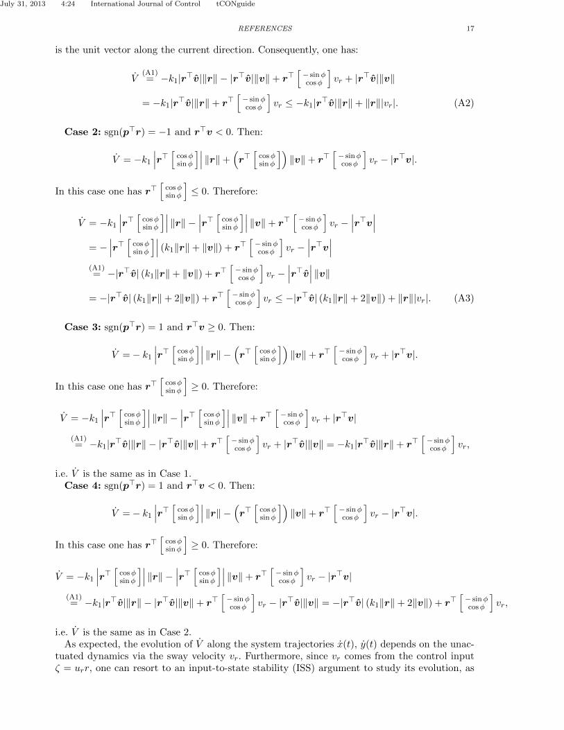
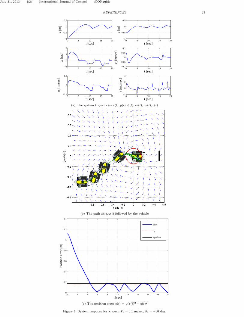
see Fig. 4(b) - 7(b).In the scenarios throughout Fig. 4 - 6, the current disturbance v is assumed to be known,

where Vc = 0.1 m/sec, and βc = −30, 30, 160 deg, respectively. In Fig. 7 the current of velocityVc = 0.1 m/sec and direction βc = 160 deg is assumed to be unknown; the only information whichis available to the switching controller is the bound ‖v‖max = 0.1. In all cases, the trajectoriesx(t), y(t) converge into the B(0, r0), where r0 = 0.15 m, and remain bounded into the ballB(0, ε), where ε = r0 + rε, with rε being a small positive number,1 see Fig. 4(b), 4(c) and Fig.7(b), 7(c). The evolution of the system trajectories x(t) is depicted in Fig. 4(a), 7(a).

It is worth noting that the main difference between the scenarios in Fig. 6, where the currentdirection βc = 160 deg is known, and Fig. 7, where the current direction βc = 160 deg isunknown, lies in the evolution of the orientation trajectories ψ(t). In particular, in the formercase and while in region G, the orientation ψ is alternately regulated between zero (when thecontrol law γ3(·) is active) and the direction φp of the vector p (when the control law γ2(·) isactive). In the latter case, the orientation ψ is regulated to zero when the vehicle is in G, butoscillates with higher frequency. This behavior is due to the fact that the system switches morefrequently between the control laws γ1(·), γ2(·) and γ3(·), since the destabilizing effect of thecurrent-induced motion along the unactuated d.o.f. drives the vehicle faster out of the set G,compared to the first case. Still, the hysteresis-based switching among the controllers (4), (11),(12) prevents the appearance of chattering when crossing the switching surface.2

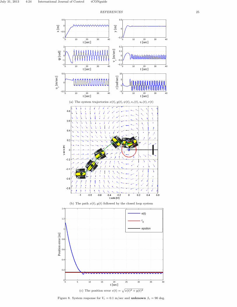
In Fig. 8 the system is subject to unknown current direction βc = 90 deg, i.e. to a currentperturbation that is vertical to the desired final orientation ψd = 0 and along the unactuatedd.o.f. at this point. The system response and the resulting path demonstrate that the positiontrajectories remain bounded around the origin, while the switching among the candidate controllaws is, as expected, much faster compared to the case in Fig. 7.

The proposed switching control strategy applies also in cases that the current direction βc is notconstant. In the scenario depicted in Fig. 9 the current direction is subject to zero-mean, uniformrandom deviation from the (unknown) nominal value βc. Fig. 9(b) illustrates the path followedby the vehicle, while Fig. 9(c) demonstrates that the position trajectories remain bounded inthe ball B(0, ε).

Finally, the efficacy of the proposed control algorithm is demonstrated in the case of a vehiclewith port-starboard symmetry only, i.e. when the system modeling includes off-diagonal elementsin the inertia and linear damping matrices. More specifically, we consider the model of a surfacevehicle (Fossen 2002) which includes the coupling between sway and yaw d.o.f. via the inertia(added mass) term m23 = m32 = −Yr = 0.3943 and the linear damping terms Yr = −4.0075,Nv = −6.6667×10−4. The system response is given in Fig. 10. As expected, the vehicle’s motionand resulting path (Fig. 10(b)) exposes a much more oscillatory behavior, compared to theprevious cases, mostly due to the inertia term m23 which affects the underactuated (sway) d.o.f..Yet, the main objective of the control design is fulfilled, since the position trajectories remainbounded in B(0, ε), as demonstrated in 10(b), while the orientation ψ(t) is regulated to zeroduring some time intervals, as demonstrated in Fig. 10(a).

7 Conclusions

This paper presented a switching control approach for the practical stabilization of an underac-tuated marine vehicle under non-vanishing, current-induced perturbations. The proposed controlscheme is a hysteresis-based switching logic among three state feedback control laws. The first

1The size of the parameter rε depends on the inertia forces and moments in subsystem Σ2. The faster the actual virtualvelocities ur(t), r(t) converge to the virtual desired values ur,d, rd, then the faster the dynamic system (1) behaves as the“virtual” closed-loop kinematic subsystem Σ1, and therefore in this case rε can be made arbitrarily small, rε → 0.2In the case of unknown current disturbances we assume that the (actual) relative linear velocities ur , u− Vc cos(βc −ψ),

vr , v − Vc sin(βc − ψ) are not online available, but rather that only the body-fixed velocities u, v can be measured. Thus,instead of ur, vr in (8) we use the “worst-case relative velocities” |u+ Vc|, |v + Vc|, respectively.


14 REFERENCES

control law employs a dipolar vector field and drives the system trajectories into a set G aroundthe origin. The other two control laws are active in G; switching between them renders the posi-tion of the vehicle practically stable, while the orientation is regulated to zero during some timeintervals. The switched system is robust, in the sense that the system trajectories converge andremain into the set G even if only a bound ‖v‖max on the current velocity is given. The proposedcontrol approach is suitable for applications where both the position and the orientation of anunderactuated vehicle is of importance, for instance in pursuing the dynamic positioning for amarine vehicle while inspecting a target of interest. Simulation results illustrate the efficacy ofthe approach. Future work can be towards the consideration of model parametric uncertainty aswell as of more challenging perturbation models.

References

Aguiar, A.P., and Pascoal, A.M. (2001), “Regulation of a Nonholonomic Autonomous Underwa-ter Vehicle with Parametric Modeling Uncertainty using Lyapunov Functions,” in Proc. ofthe 40th IEEE Conf. on Decision and Control, Dec., Orlando, FL, USA, pp. 4178–4183.

Aguiar, A.P., and Pascoal, A.M. (2002), “Global stabilization of an underactuated autonomousunderwater vehicle via logic-based switching,” in Proc. of the 41st IEEE Conf. on Decisionand Control, Dec., Las Vegas, NE, USA, pp. 3267–3272.

Aguiar, A.P., Hespanha, J.P., and Pascoal, A.M. (2007), “Switched seesaw control for the sta-bilization of underactuated vehicles,” Automatica, 43, 1997–2008.

Aguiar, A.P., and Pascoal, A.M. (2007), “Dynamic positioning and way-point tracking of un-deractuated AUVs in the presence of ocean currents,” International Journal of Control, 80,1092–1108.

Branicky, M.S. (1998), “Multiple Lyapunov Functions and Other Analysis Tools for Switchedand Hybrid Systems,” IEEE Transactions on Automatic Control, 43, 475–482.

Brockett, R.W. (1983), “Asymptotic Stability and Feedback Stabilization,” in Differential Geo-metric Control Theory eds. R. Brockett, R. Millman and H. Sussmann, Boston: Birkhauser,pp. 181–191.

Chang, W.J., Chen, G.J., and Yeh, Y.L. (2002), “Fuzzy Control of Dynamic Positioning Systemsfor Ships,” Journal of Marine Science and Technology, 10, 47–53.

Cheng, J., Yi, J., and Zhao, D. (2002), “Stabilization of an Underactuated Surface Vessel viaDiscontinuous Control,” in Proc. of the 2007 American Control Conf., Jul., NY City, NY,USA, pp. 206–211.

Do, K.D., Jiang, Z.P., Pan, J., and Nijmeijer, H. (2002), “Global output feedback universalcontroller for the stabilization and tracking of underactuated ODIN-an underwater vehicle,”in Proc. of the 41st IEEE Conf. on Decision and Control, Dec., Las Vegas, NE, USA, pp.504–509.

Dong, W., and Guo, Y. (2005), “Global Time-Varying Stabilization of Underactuated SurfaceVessel,” IEEE Trans. on Automatic Control, 50, 859–864.

Fantoni, I., Lozano, R., Mazenc, F., and Pettersen, K.Y. (2000), “Stabilization of a nonlinearunderactuated hovercraft,” Int. Journal of Robust and Nonlinear Control, 10, 645–654.

Fossen, T.I., Marine Control Systems: Guidance, Navigation and Control of Ships, Rigs andUnderwater Vehicles, Marine Cybernetics (2002).

Ghommam, J., Mnif, F., Benali, A., and Derbel, N. (2006), “Asymptotic Backstepping Stabi-lization of an Underactuated Surface Vessel,” IEEE Trans. on Control Systems Technology,14, 1150–1157.

Greytak, M., and Hover, F. (2008), “Underactuated Point Stabilization Using Predictive Mod-els with Application to Marine Vehicles,” in Proc. of the 2008 IEEE/RSJ Int. Conf. onIntelligent Robots and Systems, Sep., Nice, France, pp. 3756–3761.

Khalil, H.K., Nonlinear Systems. Third Edition, Prentice-Hall Inc. (2002).Kim, T., Basar, T., and Ha, I.J. (2002), “Asymptotic Stabilization of an Underactuated Sur-


REFERENCES 15

face Vessel via Logic-Based Control,” in Proc. of the 2002 American Control Conf., May,Anchorage, AL, USA, pp. 4678–4683.

LaValle, S.M., Planning Algorithms, Cambridge University Press (2006).Liberzon, D., Switching in Systems and Control, Birkhauser Boston (2003).Ma, B. (2009), “Global κ-exponential asymptotic stabilization of underactuated surface vessels,”

Systems and Control Letters, 58, 194–201.Mazenc, F., Pettersen, K., and Nijmeijer, H. (2002), “Global Uniform Asymptotic Stabilization

of an Underactuated Surface Vessel,” IEEE Trans. on Automatic Control, 47, 1759–1762.Nguyen, T.D., Sørensen, A.J., and Quek, S.T. (2007), “Design of hybrid controller for dynamic

positioning from calm to extreme sea conditions,” Automatica, 43, 768–785.Panagou, D., and Kyriakopoulos, K.J. (2011), “A switching control approach for the robust

practical stabilization of a unicycle-like marine vehicle under non-vanishing perturbations,”in Proc. of the 2011 IEEE International Conference on Robotics and Automation, May,Shanghai, P.R. China, pp. 1525–1530.

Panagou, D., Tanner, H.G., and Kyriakopoulos, K.J. (2011), “Control of nonholonomic systemsusing reference vector fields,” in Proc. of the 50th IEEE Conference on Decision and Controland European Control Conference, Dec., Orlando, Florida, pp. 2831–2836.

Pereira, A., Das, J., and Sukhatme, G.S. (2008), “An Experimental Study of Station Keeping onan Underactuated ASV,” in Proc. of the 2008 IEEE/RSJ Int. Conf. on Intelligent Robotsand Systems, Sep., Nice, France, pp. 3164–3171.

Pettersen, K.Y., and Egeland, O. (1999), “Time-Varying Exponential Stabilization of the Posi-tion and Attitude of an Underactuated Autonomous Underwater Vehicle,” IEEE Trans. onAutomatic Control, 44, 112–115.

Pettersen, K.Y., and Fossen, T.I. (2000), “Underactuated Dynamic Positioning of a Ship - Ex-perimental Results,” IEEE Trans. on Control Systems Technology, 8, 856–863.

Pettersen, K.Y., and Nijmeijer, H. (2001), “Semi-Global Practical Stabilization and DisturbanceAdaptation for an Underactuated Ship,” Modeling, Identification and Control, 22, 89–101.

Refsnes, J.E., Sorensen, A.J., and Pettersen, K.Y. (2007), “Output feedback control of slenderbody underwater vehicles with current estimation,” International Journal of Control, 80,1136–1150.

Refsnes, J.E., Sorensen, A.J., and Pettersen, K.Y. (2008), “Model-based output feedback controlof slender-body underactuated AUVs: Theory and Experiments,” IEEE Trans. on Controland Systems Technology, 16, 930–946.

Reyhanoglu, M. (1996), “Control and Stabilization of an Underactuated Surface Vessel,” in Proc.of the 35th IEEE Conf. on Decision and Control, Dec., Kobe, Japan, pp. 2371–2376.

Sørensen, A.J., Sagatun, S.I., and Fossen, T.I. (1996), “Design of a Dynamic Positioning SystemUsing Model-Based Control,” Control Engineering Practice, 4, 359–368.

Sørensen, A.J. (2011), “A survey of dynamic positioning control systems,” Annual Reviews inControl, 35, 123–136.

Tannuri, E.A., Agostinho, A.C., Morishita, H.M., and Jr, L.M. (2010), “Dynamic positioningsystems: An experimental analysis of sliding mode control,” Control Engineering Practice,18, 1121–1132.

Wang, W., and Clark, C.M. (2006), “Modeling and Simulation of the VideoRay Pro III Under-water Vehicle,” in Proc. of OCEANS 2006 - Asia Pacific, May, Singapore, pp. 1–7.

Wichlund, K.Y., Sordalen, O.J., and Egeland, O. (1995), “Control of Vehicles with second-orderconstraints: Underwater Vehicles,” in Proc. of the 3rd European Conf. on Control, Sep.,Rome, Italy, pp. 3086–3091.

Zhao, J., and Hill, D.J. (2008), “On stability, L2-gain and H∞ control for switched systems,”Automatica, 44, 1220–1232.


16 REFERENCES

Appendix A: Proof of Theorem 5.1

Proof In order to study the convergence of the position trajectories r(t) into a ball aroundthe origin, we think of the system Σ1 as decomposed into two subsystems with different timescales, where the state z , [ψ vr]

> constitutes the boundary-layer (fast) system, and the states

x , [x y]> constitute the reduced (slow) system. Then, the closed-loop dynamics under thecontrol law (4b) of the overall system Σ1 can be written as a singular perturbation model byconsidering the (small) parameter ε , 1

k2, for k2 sufficiently large, as follows:

x = ur cosψ − vr sinψ + Vc cosβc

y = ur sinψ + vr cosψ + Vc sinβc

εψ = −(ψ − φ)

εvr =m11

m22ur(ψ − φ) + ε

Yvm22

vr + εYv|v|

m22|vr| vr.

The boundary-layer system has one isolated root, given for ε = 0 as ψ = φ. Taking η = ψ − φ,one can easily verify that εdηdt = εψ − εφ = −(ψ − φ) − εφ ⇒ dη

dτ , −η, where εdηdt = dηdτ (Khalil

2002). This implies that ψ converges exponentially and at a very fast time scale to φ.Let us now consider the candidate Lyapunov function V = 1

2(x2 + y2) for the reduced (slow)subsystem, which is positive definite, radially unbounded and of class C1, and take the derivativeof V along the system trajectories, evaluated at the stable equilibrium η = 0 of the boundary-layer subsystem, i.e. for ψ = φ:

V = ∇V[xy

]= [ x y ]

[ur cosφ−vr sinφ+Vc cosβcur sinφ+vr cosφ+Vc sinβc

]= r>

[cosφsinφ

]ur + r>

[− sinφcosφ

]vr + r>

[Vc cosβcVc sinβc

].

Substituting the control law (4a) yields:

V = −k1

(r>[

cosφsinφ

])sgn

(r>[

cosφsinφ

])‖r‖ −

(r>[

cosφsinφ

])sgn(p>r)‖v‖+ r>

[− sinφcosφ

]vr + r>v

= −k1

∣∣∣r> [ cosφsinψ

]∣∣∣ ‖r‖ − (r> [ cosφsinφ

])sgn(p>r)‖v‖+ r>

[− sinφcosφ

]vr + r>v.

Let us check the sign of V by considering the following cases.Case 1: sgn(p>r) = −1 and r>v ≥ 0, see Fig. A1. Then:

V = −k1

∣∣∣r> [ cosφsinφ

]∣∣∣ ‖r‖+(r>[

cosφsinφ

])‖v‖+ r>

[− sinφcosφ

]vr + |r>v|.

In this case, one can easily verify out of Fig. A1 that r>[

cosφsinφ

]≤ 0. Therefore:

V = −k1


]∣∣∣ ‖r‖ − ∣∣∣r> [ cosφsinφ

]∣∣∣ ‖v‖+ r>[− sinφcosφ

]vr + |r>v|.

After some algebra one can verify that:∣∣∣r> [ cosφsinφ

]∣∣∣ =1

‖F‖

∣∣∣r> [ FpxFpy

]∣∣∣ (3)=

1

‖F‖(x2 + y2

)|r>v| = |r>v|, (A1)

where the norm of the vector field is ‖F‖ ,√

F2px + F2

py(3)= x2 + y2, and v = [cosβc sinβc]

>


REFERENCES 17

is the unit vector along the current direction. Consequently, one has:

V(A1)= −k1|r>v|‖r‖ − |r>v|‖v‖+ r>

[− sinφcosφ

]vr + |r>v|‖v‖

= −k1|r>v|‖r‖+ r>[− sinφcosφ

]vr ≤ −k1|r>v|‖r‖+ ‖r‖|vr|. (A2)

Case 2: sgn(p>r) = −1 and r>v < 0. Then:

V = −k1


]∣∣∣ ‖r‖+(r>[

cosφsinφ

])‖v‖+ r>

[− sinφcosφ

]vr − |r>v|.

In this case one has r>[

cosφsinφ

]≤ 0. Therefore:

V = −k1


]∣∣∣ ‖r‖ − ∣∣∣r> [ cosφsinφ


]vr −

∣∣∣r>v∣∣∣= −


]∣∣∣ (k1‖r‖+ ‖v‖) + r>[− sinφcosφ

]vr −

∣∣∣r>v∣∣∣(A1)= −|r>v| (k1‖r‖+ ‖v‖) + r>

[− sinφcosφ

]vr −

∣∣∣r>v∣∣∣ ‖v‖= −|r>v| (k1‖r‖+ 2‖v‖) + r>

[− sinφcosφ

]vr ≤ −|r>v| (k1‖r‖+ 2‖v‖) + ‖r‖|vr|. (A3)

Case 3: sgn(p>r) = 1 and r>v ≥ 0. Then:

V =− k1



])‖v‖+ r>

[− sinφcosφ

]vr + |r>v|.


cosφsinφ

]≥ 0. Therefore:

V = −k1


]∣∣∣ ‖r‖ − ∣∣∣r> [ cosφsinφ


]vr + |r>v|

(A1)= −k1|r>v|‖r‖ − |r>v|‖v‖+ r>

[− sinφcosφ

]vr + |r>v|‖v‖ = −k1|r>v|‖r‖+ r>

[− sinφcosφ

]vr,

i.e. V is the same as in Case 1.Case 4: sgn(p>r) = 1 and r>v < 0. Then:

V =− k1



])‖v‖+ r>

[− sinφcosφ

]vr − |r>v|.


cosφsinφ

]≥ 0. Therefore:

V = −k1


]∣∣∣ ‖r‖ − ∣∣∣r> [ cosφsinφ


]vr − |r>v|

(A1)= −k1|r>v|‖r‖ − |r>v|‖v‖+ r>

[− sinφcosφ

]vr − |r>v|‖v‖ = −|r>v| (k1‖r‖+ 2‖v‖) + r>

[− sinφcosφ

]vr,

i.e. V is the same as in Case 2.As expected, the evolution of V along the system trajectories x(t), y(t) depends on the unac-

tuated dynamics via the sway velocity vr. Furthermore, since vr comes from the control inputζ = urr, one can resort to an input-to-state stability (ISS) argument to study its evolution, as


18 REFERENCES

follows: Consider the candidate ISS-Lyapunov function Vv = 12vr

2 and take its time derivative

Vv = −m11

m22vr(urr)−

(|Yv|m22

vr2 +|Yv|v||m22

|vr| vr2

),

where Yv, Yv|v| < 0 and the function w(vr) = |Yv|m22

vr2 +

|Yv|v||m22|vr| vr2 is positive definite. Take

θ ∈ (0, 1), then:

Vv = −m11

m22vr(urr)− (1− θ)w(vr)− θw(vr)⇒ Vv ≤ −(1− θ)w(vr), ∀vr : −m11

m22vr(urr)− θw(vr) ≤ 0.

If the control input ζ = urr is bounded, |ζ| ≤ ζb, then

Vv ≤ −(1− θ)w(vr), ∀|vr| : |Yv||vr|+ |Yv|v|||vr|2 >m11

θζb.

Then, the subsystem (1e) is ISS w.r.t. ζ (Khalil 2002, Thm 4.19), which essentially expressesthat for any bounded input ζ = urr, the linear velocity vr(t) will be ultimately bounded by aclass K function of supt>0 |ζ(t)|. If furthermore ζ(t) = ur(t)r(t) converges to zero as t → ∞,then vr(t) converges to zero as well (Khalil 2002).

At this point, note that the control input r , −k2η is bounded and converges to zero at avery fast time scale, since the orientation error η = 0 is the exponentially stable equilibriumof the boundary-layer subsystem. This further implies that, for sufficiently large k2, the swayvelocity vr converges to zero very fast, compared to the remaining slow dynamics of x(t), y(t).Consequently, the positive terms in (A2), (A3) vanish much faster than the negative terms,yielding V ≤ 0, where V = 0 if r>v = 0 or if r = 0.

Consequently, for r>v 6= 0, any initial r(0) and any 0 < r0 < ‖r(0)‖, one has that V isnegative in the set {r

∣∣ 12r0

2 ≤ V (‖r‖) ≤ 12‖r(0)‖2}, which verifies that r(t) enters the set

{r∣∣ V (r) ≤ 1

2r02}, or equivalently, r(t) enters the ball B(0, r0). Finally, note that the case

r>v = 0 where V = 0 does not affect the convergence of the system into B(0, r0), since thesystem can not identically stay in this set. �

Appendix B: Proof of Theorem 5.2

Proof Under the control law (5) the system trajectories q(t) first reach the boundary ∂G1G2,

and then reach the boundary ∂G2B .To verify the first argument, i.e. that the system trajectories reach the boundary ∂G1G2

,consider the Lyapunov-like function:

V21 = r>v +1

2(ψ − φp)2 = Vc(x cosβc + y sinβc) +

1

2(ψ − φp)2,

which is positive everywhere in G1, since there one has r>v ≥ 0, and becomes zero on theboundary ∂G1G2

for ψ = φp, and take its time derivative along the system trajectories:

V21 = [ Vc cosβc Vc sinβc ][xy

]+ (ψ − φp)ψ

(1)= v>

[cosψsinψ

]ur + v>

[− sinψcosψ

]vr + ‖v‖2 + (ψ − φp)r

(5)= −k3 sgn(cosβc)‖v‖v>

[cosψsinψ

]+ v>

[− sinψcosψ

]vr + ‖v‖2 − k4(ψ − φp)2.

Let us consider the following cases.


REFERENCES 19

(1) sgn(cosβc) = −1. It is reasonable to assume that, under the control law (4), the vehicle

has reached G1 with v>[

cosψsinψ

]< 0. Then:

V21 = −k3

∣∣∣v> [ cosψsinψ

]∣∣∣ ‖v‖+ ‖v‖2 + v>[− sinψcosψ

]vr − k4(ψ − φp)2 =

= ‖v‖(‖v‖ − k3


]∣∣∣)+ v>[− sinψcosψ

]vr − k4(ψ − φp)2,

where the first term is < 0 for ‖v‖ < k3


]∣∣∣ ⇒ k3 > 1. Furthermore, one has

that ζ = urr → 0, since r → 0 (via ψ → (φp = ψe)), yielding vr → 0. Note also

that V21 = 0 ⇔ {k3 = 1 and vr = 0 and ψ = φp}. Therefore, for k3 > 1 the systemtrajectories starting in G1 enter the region G2.

(2) sgn(cosβc) = 1. Similarly one can take v>[

cosψsinψ

]> 0 and follow the same procedure to

yield that for k3 > 1, the system trajectories starting in G1 enters the region G2.

Finally, to verify the second argument, i.e. that the system trajectories reach the boundary∂G2B , consider the Lyapunov-like function:

V22 = r02 − ‖r‖2 = r0

2 − (x2 + y2),

which is positive for r ∈ G2 and zero on ∂G2B , and take its time derivative along the systemtrajectories:

V22 = −2r>[

cosψsinψ

]ur − 2r>

[− sinψcosψ

]vr − 2r>v

(5)= 2r>

[cosψsinψ

]sgn(cosβc)k3‖v‖ − 2r>

[− sinψcosψ

]vr − 2r>v.

Let us consider the following cases.

(1) sgn(cosβc) = −1, then one has: r>v < 0 and r>[

cosψsinψ

]> 0. Consequently:

V22 = −2k3r>[

cosψsinψ

]‖v‖ − 2r>

[− sinψcosψ

]vr − 2r>v =

− 2k3

∣∣∣r> [ cosψsinψ

]∣∣∣ ‖v‖ − 2r>[− sinψcosψ

]vr + 2

∣∣∣r>v∣∣∣≤ −2k3


]∣∣∣ ‖v‖ − 2r>[− sinψcosψ

]vr + 2‖r‖‖v‖

= 2‖v‖(‖r‖ − k3


]∣∣∣)− 2r>[− sinψcosψ

]vr,

where the first term is < 0 for ‖r‖ < k3


]∣∣∣ ≤ ‖r‖ ⇒ k3 > 1. Thus, for k3 > 1,

the system trajectories q(t) hit the boundary ∂G2B and enters B.

(2) sgn(cosβc) = 1, then one has: r>v < 0 and r>[

cosψsinψ

]< 0. Following the same procedure,

one eventually gets that V22 < 0⇒ k3 > 1.

�


20 REFERENCES

Appendix C: Proof of Theorem 5.3

Proof Let us first prove that the system trajectories enter the set G1, by considering the candi-date Lyapunov-like function V31 = −r>v, which is positive for r ∈ G2 and zero on ∂G2G1

. Thetime derivative along the system trajectories is:

V31(1)= −Vc cosβc(ur cosψ − vr sinψ + Vc cosβc)− Vc sinβc(ur sinψ + vr cosψ + Vc sinβc)

(6)= −‖v‖2 − v>

[− sinψcosψ

]vr,

where vr → 0 since ζ = urr → 0. Consequently, the system trajectories q(t) enter the set G1.Finally, for r ∈ G1 take the candidate Lyapunov-like function V32 = r0

2 − x2 − y2, where

V32 = −‖v‖2 − v>[− sinψcosψ

]vr < 0,

to verify that the system trajectories q(t) enter the set A. �

Appendix D: Proof of Theorem 5.6

Proof Under the feedback linearization transformation (8), the corresponding dynamic equations(1d), (1f) read ur = α, r = β, respectively, where α, β are the new control inputs. Consider thecandidate Lyapunov function

Vτ =1

2(ur − ur,d(·))2 +

1

2(r − rd(·))2 ,

and take its time derivative as Vτ = (ur − ur,d(·))(ur− (∇ur,d(·))q

)+ (r− rd(·))

(r− (∇rd(·))q

).

Then, under the control inputs (9) one gets

Vτ = −ku(ur − urd(·))2 − kr(r − rd(·))2 ≤ −2 min{ku, kr}Vτ ,

which verifies that the actual velocities ur(t), r(t) are GES to the virtual velocities ur,d(·), rd(·),respectively. �


REFERENCES 21

0 5 10 15 20−1

−0.5

0

0.5

t [sec]

x [m

]

0 5 10 15 20−1

−0.5

0

0.5

t [sec]

y [m

]

0 5 10 15 20−1

0

1

2

t [sec]

ψ [

rad]

0 5 10 15 20−0.1

−0.05

0

0.05

0.1

t [sec]

v r [m

/sec

]

0 5 10 15 20−0.5

0

0.5

t [sec]

u r [m

/sec

]

0 5 10 15 20−2

0

2

4

t [sec]

r [r

ad/s

ec]

(a) The system trajectories x(t), y(t), ψ(t), vr(t), ur(t), r(t)

(b) The path x(t), y(t) followed by the vehicle

0 2 4 6 8 10 12 14 16 18 200

0.2

0.4

0.6

0.8

1

1.2

1.4

t [sec]

Posi

tion

erro

r [m

]

e(t)

r0

epsilon

(c) The position error e(t) =√x(t)2 + y(t)2

Figure 4. System response for known Vc = 0.1 m/sec, βc = −30 deg.


22 REFERENCES

0 5 10 15 20−1

−0.5

0

0.5

t [sec]

x [m

]

0 5 10 15 20−0.5

0

0.5

t [sec]

y [m

]

0 5 10 15 20−0.5

0

0.5

1

t [sec]

ψ [

rad]

0 5 10 15 20−0.05

0

0.05

t [sec]

v r [m

/sec

]

0 5 10 15 20−0.5

0

0.5

t [sec]

u r [m

/sec

]

0 5 10 15 20−5

0

5

t [sec]

r [r

ad/s

ec]



0 2 4 6 8 10 12 14 16 18 200

0.2

0.4

0.6

0.8

1

1.2

1.4

t [sec]

Posi

tion

erro

r [m

]

e(t)

r0

epsilon


Figure 5. System response for known Vc = 0.1 m/sec, βc = 30 deg.


REFERENCES 23

0 10 20 30 40−1

−0.5

0

0.5

t [sec]

x [m

]

0 10 20 30 40−0.5

0

0.5

t [sec]

y [m

]

0 10 20 30 40−1

0

1

2

t [sec]

ψ [

rad]

0 10 20 30 40−0.1

−0.05

0

0.05

0.1

t [sec]

v r [m

/sec

]

0 10 20 30 40−0.5

0

0.5

t [sec]

u r [m

/sec

]

0 10 20 30 40−1

0

1

2

t [sec]

r [r

ad/s

ec]



0 5 10 15 20 25 30 35 400

0.2

0.4

0.6

0.8

1

1.2

1.4

t [sec]

Posi

tion

erro

r [m

]

e(t)

r0

epsilon


Figure 6. System response for known Vc = 0.1 m/sec, βc = 160 deg.


24 REFERENCES

0 10 20 30 40−1

−0.5

0

0.5

t [sec]

x [m

]

0 10 20 30 40−0.5

0

0.5

t [sec]

y [m

]

0 10 20 30 40−1

−0.5

0

0.5

1

t [sec]

ψ [

rad]

0 10 20 30 40−0.1

−0.05

0

0.05

0.1

t [sec]

v r [m

/sec

]

0 10 20 30 40−0.5

0

0.5

t [sec]

u r [m

/sec

]

0 10 20 30 40−5

0

5

t [sec]

r [r

ad/s

ec]



0 5 10 15 20 25 30 35 400

0.2

0.4

0.6

0.8

1

1.2

1.4

t [sec]

Posi

tion

erro

r [m

]

e(t)

r0

epsilon


Figure 7. System response for Vc = 0.1 m/sec and unknown βc = 160 deg.


REFERENCES 25

0 10 20 30 40−1

−0.5

0

0.5

t [sec]

x [m

]

0 10 20 30 40−0.5

0

0.5

t [sec]

y [m

]

0 10 20 30 40−2

−1

0

1

2

t [sec]

ψ [

rad]

0 10 20 30 40−0.2

−0.1

0

0.1

0.2

t [sec]

v r [m

/sec

]

0 10 20 30 40−0.5

0

0.5

t [sec]

u r [m

/sec

]

0 10 20 30 40−5

0

5

10

t [sec]

r [r

ad/s

ec]


(b) The path x(t), y(t) followed by the closed loop system

0 5 10 15 20 25 30 35 400

0.2

0.4

0.6

0.8

1

1.2

1.4

t [sec]

Posi

tion

erro

r [m

]

e(t)

r0

epsilon


Figure 8. System response for Vc = 0.1 m/sec and unknown βc = 90 deg.


26 REFERENCES

0 10 20 30 40−1

−0.5

0

0.5

t [sec]

x [m

]

0 10 20 30 40−1

−0.5

0

0.5

t [sec]

y [m

]

0 10 20 30 40−1

−0.5

0

0.5

1

t [sec]

ψ [

rad]

0 10 20 30 40−0.1

−0.05

0

0.05

0.1

t [sec]

v r [m

/sec

]

0 10 20 30 40−0.5

0

0.5

t [sec]

u r [m

/sec

]

0 10 20 30 40−5

0

5

t [sec]

r [r

ad/s

ec]



0 5 10 15 20 25 30 35 400

0.2

0.4

0.6

0.8

1

1.2

1.4

t [sec]

Posi

tion

erro

r [m

]

e(t)

r0

epsilon


Figure 9. System response for unknown v, such that ‖v‖max = 0.1 m/sec, under varying current direction βc.


REFERENCES 27

0 10 20 30 40−1

−0.5

0

0.5

t [sec]

x [m

]

0 10 20 30 40−1

−0.5

0

0.5

t [sec]

y [m

]

0 10 20 30 40−4

−2

0

2

t [sec]ψ

[ra

d]0 10 20 30 40

−0.5

0

0.5

1

t [sec]

v r [m

/sec

]

0 10 20 30 40−0.4

−0.2

0

0.2

0.4

t [sec]

u r [m

/sec

]

0 10 20 30 40−5

0

5

10

t [sec]

r [r

ad/s

ec]


−1 −0.8 −0.6 −0.4 −0.2 0 0.2 0.4 0.6−0.8

−0.6

−0.4

−0.2

0

0.2

0.4

0.6

0.8

x axis [m]

y ax

is [m

]


0 5 10 15 20 25 30 35 400

0.2

0.4

0.6

0.8

1

1.2

1.4

t [sec]

Posi

tion

erro

r [m

]

e(t)

r0

epsilon


Figure 10. System response for Vc = 0.1 m/sec and unknown βc = 90 deg with off-diagonal inertia and dampingelements.


28 REFERENCES

Figure A1. System configuration w.r.t. the dipolar field (3)

RESEARCH ARTICLE Dynamic Positioning for an Underactuated ...

Documents

Transcript of RESEARCH ARTICLE Dynamic Positioning for an Underactuated ...