Research Article Control-Scheduling Codesign...

Research ArticleControl-Scheduling Codesign Exploiting Trade-Off betweenTask Periods and Deadlines

Hyun-Jun Cha,1 Woo-Hyuk Jeong,2 and Jong-Chan Kim1

1Graduate School of Automotive Engineering, Kookmin University, 77 Jeongneung-ro, Seongbuk-gu, Seoul 02707, Republic of Korea2Department of Computer Science, Kookmin University, 77 Jeongneung-ro, Seongbuk-gu, Seoul 02707, Republic of Korea

Correspondence should be addressed to Jong-Chan Kim; [email protected]

Received 1 January 2016; Revised 22 March 2016; Accepted 27 March 2016

Academic Editor: Qixin Wang

Copyright © 2016 Hyun-Jun Cha et al. This is an open access article distributed under the Creative Commons Attribution License,which permits unrestricted use, distribution, and reproduction in any medium, provided the original work is properly cited.

A control task’s performance heavily depends on its sampling frequency and sensing-to-actuation delay. More frequent sampling,that is, shorter period, improves the control performance. Similarly, shorter delay also has a positive effect. Moreover, schedulabilityis also a function of periods and deadlines. By taking into account the control performance and schedulability at the same time,this paper defines a period and deadline selection problem for fixed-priority systems. Our problem is to find the optimal periodsand deadlines for given tasks that maximize the overall system performance. As our solution, this paper presents a novel heuristicalgorithm that finds a high-quality suboptimal solution with very low complexity, whichmakes the algorithm practically applicableto large size task sets.

1. Introduction

In a cyberphysical system (CPS), real-time control systemsmonitor and control physical systems (i.e., target plants) withprecise control performance requirements and tight resourceconstraints. When designing such a system, two differentapproaches can be applied. First, the traditional approachseparates the control design phase and implementation phasesuch that scheduling parameters such as sampling rates aredetermined in the control design phase without consideringthe scheduling issue.The second approach, known as control-scheduling codesign, takes into account both the control per-formance and task scheduling simultaneously for the purposeof enhancing control performance with limited resources [1–4].This paper advocates the second approachwhen designinga CPS.

Performance of a real-time control system in a CPSdepends on not only its functional correctness but alsoits scheduling parameters such as sampling frequency. Withmore frequent sensing and actuation, more accurate con-trol results can be obtained [5]. Certainly, this perfor-mance enhancement is at the cost of increased comput-ing demands. Another important but often ignored timingproperty is the delay between sensing and actuation, that is,

input-output delay. Since a shorter delay means more recentsensing data has been used to produce the actuation value,it can provide higher control performance [5]. Then, oneinteresting observation is that a task’s period, that is, inverseof sampling frequency, can be lengthened without hurtingthe control performance if we can somehow reduce the delay.To maintain a task’s delay within a certain range, the desiredmaximum delay should be used as the relative deadline in theschedulability check. If the schedulability check passes, thetask’s input-output delay is guaranteed less than the relativedeadline. One more timing attribute we have to discuss isjitter, which is the amount of uncertain variation of samplingtime or input-output delay, called sampling jitter and input-output jitter, respectively. Generally, large jitter has negativeeffects on the control performance even though the effectis not that significant as the input-output delay [6]. Evenregarding jitters, a shorter relative deadline also gives tighterupper bounds of the sampling jitter and input-output jittersuch that a better control result can be produced [6]. As aresult, the control performance can be enhanced by eitherway of shorter periods or shorter deadlines, and periodsand deadlines have a trade-off relation in terms of controlperformance.

Hindawi Publishing CorporationMobile Information SystemsVolume 2016, Article ID 3414816, 11 pageshttp://dx.doi.org/10.1155/2016/3414816

2 Mobile Information Systems

Besides control performance, schedulability is also heav-ily affected by periods and deadlines of the tasks. Generallyspeaking, longer periods and longer deadlines both makethe system more schedulable, however, at the cost of areduced control performance. In other words, a better controlperformance can be obtained with a lower chance of beingschedulable. Moreover, similar to the control performancecase, periods and deadlines aremutually tradable tomaintainschedulability.Therefore, it is important to select proper peri-ods and deadlines which satisfy both the control performanceand the schedulability. For this control-scheduling codesignissue, an optimization problem can be formulatedwhich findsthe best feasible periods and deadlines for given tasks thatmaximize the overall system performance.

In the literature, with a similar motivation, period selec-tion problem has been extensively studied [7–10] for bothdynamic and fixed-priority scheduling algorithms. However,period and deadline selection problem, which this paperis dealing with, has gathered relatively little attention andonly the dynamic-priority case has been studied [6, 11].With this motivation, targeting fixed-priority systems, thispaper proposes a novel task set synthesis algorithm thatfinds the proper periods and deadlines which maximize theoverall system performance while guaranteeing the systemschedulability. Since, even with a small number of tasks,finding the optimal solution is intractable due to the hugesolution space to be searched, our algorithm is basicallystructured as a search-based heuristic algorithm. As will beshown in Section 6, our algorithmhas a linear complexity andfinds a high-quality suboptimal solution evenwith a large taskset.

For the quantitative analysis of control performancewith varying periods and deadlines, we also conduct ameasurement study with an automotive control application.The measured control performance of the task is defined as anonlinear and nonconvex function of period and deadline.This function is used as an input to our heuristic algo-rithm.

This paper’s contribution can be summarized as follows:

(i) We identify and demonstrate the trade-off relationbetween period and deadline in terms of control per-formance through actual experimental studies withan automotive control application.

(ii) Exploiting the above trade-off relation, a novel task setsynthesis algorithm is proposed, which heuristicallyfinds near-optimal feasible (period and delay) com-binations maximizing the overall control perform-ance.

The rest of our paper is organized as follows. The nextsection briefly explains related work. Section 3 presents briefbackground knowledge and formally describes our problem.In Section 4, the trade-off relation of control performanceis formally described. Section 5 presents our heuristic algo-rithm for the period and deadline selection problem. Theexperimental results are presented in Section 6. Finally,Section 7 concludes this paper.

2. Related Work

Control-scheduling codesign problem has been extensivelystudied in the literature. Seto et al. [7] first defined the periodselection problem assuming that the control performancecan be expressed as an exponential decay function of thesampling period and the tasks are scheduled using dynamic-priority methods. The problem is extended to fixed-prioritysystems by Seto et al. [8] by finding the finite set of feasibleperiod ranges using a branch and bound-based integerprogramming method. In their work, the cost function isassumed to be a monotonically increasing function of taskperiod. Later, Bini and Di Natale [9] proposed a fasteralgorithm that finds a suboptimal period assignment, whichcan be used for a task set of practical size that was intractableby previous methods due to its high computing demands.Recently, Du et al. [12] proposed an analytical solution usingthe method of Lagrange multipliers and an online algorithmfor the overloaded situation.

The common assumption of the above researches regard-ing the period selection problem is that the control per-formance is only affected by the sampling rate, that is,task period, of the controller. However, the delay betweensensing and actuation also has a significant effect on thecontrol performance. With this motivation, Bini and Cervin[10] incorporated each task’s sensing to actuation delayinto the cost function. In their work, in order to find theoptimal period assignment, cost functions are approximatedas linear functions of period and delay, and the delay is alsoapproximated assuming the fluid model scheduler. Throughthese approximations, they proposed an analytical solu-tion.

Wu et al. [6] further enhanced the algorithm by findingtask periods and deadlines altogether for EDF scheduledsystems. As a result, the problem had become a period anddeadline selection problem. They showed that, by regulatingrelative deadlines of tasks, we can upper-limit the amount ofdelays and jitter each task can experience. In their work, thecost function is assumed to be a nonlinear function whichincreases in both period and deadline of tasks. A two-stepapproach was presented which first fixes periods and triesto minimize deadlines using unused resources. Recently, Tanet al. [11] proposed a new algorithm which simultaneouslyadjusts periods and deadlines assuming EDF scheduling andLGQ controller tasks. They showed that the new algorithmis more robust with different workloads than the previousmethod.

Despite the above researches, however, compared to theperiod selection problem, the period and deadline selec-tion problem has gained less attention even though it hasmore flexibility to enhance control performance with scarceresources. Moreover, only EDF scheduling is consideredin the period and deadline selection problem due to itsease of schedulability analysis, though the fixed-priorityscheduling is more commonly used in the practice. Onthe contrary, this paper is dealing with the period anddeadline selection problem under the fixed-priority schedul-ing.

Mobile Information Systems 3

Vehicle centerpoint

Lane centerline

Lateralerror

Figure 1: Lane keeping assist system. Its system error is defined asthe lateral distance between the vehicle center point and the lanecenter line.

3. Background and Problem Description

3.1. SystemModel. This paper considers a systemwith 𝑛 inde-pendent periodic real-time tasks {𝜏

1, 𝜏2, . . . , 𝜏

𝑛}, which con-

trol 𝑛 different plants, respectively. The tasks are scheduledby the fixed-priority scheduler and the priorities are assignedaccording to the Deadline Monotonic (DM) order. Each 𝜏

𝑖is

characterized by the following scheduling parameters:

(i) 𝐶𝑖: the worst-case execution time (WCET).

(ii) 𝑇𝑖: the sampling period.

(iii) 𝐷𝑖: the relative deadline.

From the above, 𝐶𝑖is a known parameter decided by the

control code, whereas 𝑇𝑖and 𝐷

𝑖are operational parameters

which can be controlled by system designers. Regardingdeadlines, this paper considers only constrained deadlineswhere 𝐷

𝑖is always less than or equal to 𝑇

𝑖. During system

execution, each 𝜏𝑖generates infinite sequence of periodic

jobs 𝜏𝑖,1, 𝜏𝑖,2, . . . with its period 𝑇

𝑖, which controls its corre-

sponding target plant by (i) sensing the state of the plant, (ii)calculating the actuation values, and (iii) actuating the plant.

3.2. Control Performance as a Function of Period andDeadline.When defining the performance of a controller, variousmetrics can be used, such as transient response time andsteady-state accuracy [6, 13]. In some cases, even the energyconsumption can be a control performance metric [7].Among the various control performance metrics, this paperchooses the system error as our optimization target. Systemerror is defined as the difference between the desired state andthe actual state of the plant [6].This can be thought of as howwell the plant is acting following the controller’s intention.

More specifically, let us take the lane keeping assist system(LKAS) as an example. In a modern vehicle, LKAS controlsthe steering angle such that the vehicle is able to follow thecenter of its lane.Then, the system error can be defined as thelateral error between the center of the vehicle and the centerof the lane, which is illustrated in Figure 1. Since this systemerror also varies along with time 𝑡, we further define theworst-case system error as the largest lateral error the vehiclecan experience during its driving.More interested readers arereferred to [14].

Following the notation in [6], each task’s control perfor-mance is defined as a function of its period and deadline,which is denoted by

𝐽𝑖(𝑇𝑖, 𝐷𝑖) . (1)

Generally, 𝐽𝑖(𝑇𝑖, 𝐷𝑖) is defined as a nonlinear cost function

which increases in both𝑇𝑖and𝐷

𝑖; that is, if period or deadline

increases, system error always increases.The intuition behindthis assumption will be discussed in Section 4. We assumethat 𝐽

𝑖(𝑇𝑖, 𝐷𝑖) is not continuous but discrete in both 𝑇

𝑖

and 𝐷𝑖, which are also constrained within [𝑇min

𝑖, 𝑇

max𝑖] and

[𝐷min𝑖, 𝐷

max𝑖], respectively.

Besides each task’s system error, the overall system erroris denoted by

𝐽 (𝑇,𝐷) , (2)

where 𝑇 is the vector of 𝑇𝑖’s and 𝐷 is the vector of 𝐷

𝑖’s. For

the notational simplicity, 𝐽(𝑇,𝐷) is shortened to 𝐽 as in thefollowing:

𝐽 = ∑

1≤𝑖≤𝑛

𝑤𝑖𝐽𝑖(𝑇𝑖, 𝐷𝑖) , (3)

where 𝐽 is defined as a weighted sum of 𝐽𝑖(𝑇𝑖, 𝐷𝑖)’s and𝑤

𝑖is a

user-defined weight constant for the purpose of normalizingeach 𝐽

𝑖(𝑇𝑖, 𝐷𝑖) to a desired range. Now, the system’s overall

system error can be obtained by giving every task’s period anddeadline.

3.3. Problem Description. Assuming the above concepts andnotations, this subsection describes our period and deadlineselection problem, which can be formally defined as follows.

Problem Description. For a given task set {𝜏1, 𝜏2, . . . , 𝜏

𝑛}, each

𝜏𝑖’s 𝐶𝑖and 𝐽𝑖(𝑇𝑖, 𝐷𝑖) are given a priority. Then, our problem

is to find the optimal 𝑇 = (𝑇1, 𝑇2, . . . , 𝑇

𝑛) and 𝐷 =

(𝐷1, 𝐷2, . . . , 𝐷

𝑛) such that the overall system error 𝐽(𝑇,𝐷) is

minimized while guaranteeing every 𝜏𝑖’s schedulability.

Since it is assumed that 𝐽𝑖(𝑇𝑖, 𝐷𝑖) is not continuous, we do

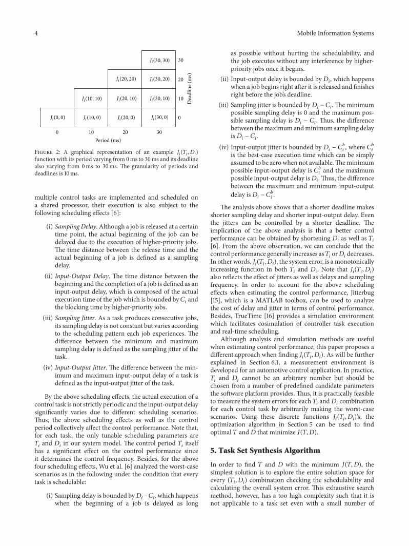
not try to make an analytical solution for our optimizationproblem. Instead, we formulate our problem as a combina-torial optimization problem. Figure 2 shows a graphical rep-resentation of an example 𝐽

𝑖(𝑇𝑖, 𝐷𝑖) with 10 discrete (𝑇

𝑖, 𝐷𝑖)

combinations. Note that since we only consider constraineddeadlines, the left upper triangular matrix is not consideredat all.

4. How Scheduling AffectsControl Performance

This section deals with the rationale behind the definition of𝐽𝑖(𝑇𝑖, 𝐷𝑖), which is introduced in Section 3.2. It is claimed in

many literatures that the control performance of a task can bedefined as a function of the task period anddeadline [6, 10, 11].If the control system is composed of only a single periodictask, it should be strictly periodic and the input-output delayis simply bounded by 𝐶

𝑖. Thus, the control performance

should be defined as a function of 𝑇𝑖and 𝐶

𝑖. However, when


0

0

10

10

20

20

30

30Period (ms)

Dea

dlin

e (m

s)

Ji(30, 30)

Ji(20, 20) Ji(30, 20)

Ji(10, 10) Ji(20, 10) Ji(30, 10)

Ji(0, 0) Ji(10, 0) Ji(20, 0) Ji(30, 0)

Figure 2: A graphical representation of an example 𝐽𝑖(𝑇𝑖, 𝐷𝑖)

function with its period varying from 0ms to 30ms and its deadlinealso varying from 0ms to 30ms. The granularity of periods anddeadlines is 10ms.

multiple control tasks are implemented and scheduled ona shared processor, their execution is also subject to thefollowing scheduling effects [6]:

(i) Sampling Delay. Although a job is released at a certaintime point, the actual beginning of the job can bedelayed due to the execution of higher-priority jobs.The time distance between the release time and theactual beginning of a job is defined as a samplingdelay.

(ii) Input-Output Delay. The time distance between thebeginning and the completion of a job is defined as aninput-output delay, which is composed of the actualexecution time of the job which is bounded by 𝐶

𝑖and

the blocking time by higher-priority jobs.(iii) Sampling Jitter. As a task produces consecutive jobs,

its sampling delay is not constant but varies accordingto the scheduling pattern each job experiences. Thedifference between the minimum and maximumsampling delay is defined as the sampling jitter of thetask.

(iv) Input-Output Jitter. The difference between the min-imum and maximum input-output delay of a task isdefined as the input-output jitter of the task.

By the above scheduling effects, the actual execution of acontrol task is not strictly periodic and the input-output delaysignificantly varies due to different scheduling scenarios.Thus, the above scheduling effects as well as the controlperiod collectively affect the control performance. Note that,for each task, the only tunable scheduling parameters are𝑇𝑖and 𝐷

𝑖in our system model. The control period 𝑇

𝑖itself

has a significant effect on the control performance sinceit determines the control frequency. Besides, for the abovefour scheduling effects, Wu et al. [6] analyzed the worst-casescenarios as in the following under the condition that everytask is schedulable:

(i) Sampling delay is bounded by𝐷𝑖−𝐶𝑖, which happens

when the beginning of a job is delayed as long

as possible without hurting the schedulability, andthe job executes without any interference by higher-priority jobs once it begins.

(ii) Input-output delay is bounded by 𝐷𝑖, which happens

when a job begins right after it is released and finishesright before the job’s deadline.

(iii) Sampling jitter is bounded by𝐷𝑖− 𝐶𝑖. The minimum

possible sampling delay is 0 and the maximum pos-sible sampling delay is 𝐷

𝑖− 𝐶𝑖. Thus, the difference

between themaximum andminimum sampling delayis𝐷𝑖− 𝐶𝑖.

(iv) Input-output jitter is bounded by 𝐷𝑖− 𝐶𝑏

𝑖, where 𝐶𝑏

𝑖

is the best-case execution time which can be simplyassumed to be zero when not available.Theminimumpossible input-output delay is 𝐶𝑏

𝑖and the maximum

possible input-output delay is𝐷𝑖. Thus, the difference

between the maximum and minimum input-outputdelay is𝐷

𝑖− 𝐶𝑏

𝑖.

The analysis above shows that a shorter deadline makesshorter sampling delay and shorter input-output delay. Eventhe jitters can be controlled by a shorter deadline. Theimplication of the above analysis is that a better controlperformance can be obtained by shortening 𝐷

𝑖as well as 𝑇

𝑖

[6]. From the above observation, we can conclude that thecontrol performance generally increases as𝑇

𝑖or𝐷𝑖decreases.

In other words, 𝐽𝑖(𝑇𝑖, 𝐷𝑖), the system error, is a monotonically

increasing function in both 𝑇𝑖and 𝐷

𝑖. Note that 𝐽

𝑖(𝑇𝑖, 𝐷𝑖)

also reflects the effect of jitters as well as delays and samplingfrequency. In order to account for the above schedulingeffects when estimating the control performance, Jitterbug[15], which is a MATLAB toolbox, can be used to analyzethe cost of delay and jitter in terms of control performance.Besides, TrueTime [16] provides a simulation environmentwhich facilitates cosimulation of controller task executionand real-time scheduling.

Although analysis and simulation methods are usefulwhen estimating control performance, this paper proposes adifferent approach when finding 𝐽

𝑖(𝑇𝑖, 𝐷𝑖). As will be further

explained in Section 6.1, a measurement environment isdeveloped for an automotive control application. In practice,𝑇𝑖and 𝐷

𝑖cannot be an arbitrary number but should be

chosen from a number of predefined candidate parametersthe software platform provides. Thus, it is practically feasibleto measure the system errors for each 𝑇

𝑖and𝐷

𝑖combination

for each control task by arbitrarily making the worst-casescenarios. Using these discrete functions 𝐽

𝑖(𝑇𝑖, 𝐷𝑖)’s, the

optimization algorithm in Section 5 can be used to findoptimal 𝑇 and𝐷 that minimize 𝐽(𝑇,𝐷).

5. Task Set Synthesis Algorithm

In order to find 𝑇 and 𝐷 with the minimum 𝐽(𝑇,𝐷), thesimplest solution is to explore the entire solution space forevery (𝑇

𝑖, 𝐷𝑖) combination checking the schedulability and

calculating the overall system error. This exhaustive searchmethod, however, has a too high complexity such that it isnot applicable to a task set even with a small number of


tasks like five or six tasks. The computational feasibility ofthe exhaustive search algorithm will be further discussedin Section 6.2. Instead, this section proposes an alternativeheuristic algorithm that finds a suboptimal result, however,with a very low computational complexity. Even with thislow complexity, our solution can find a very-high-qualitysolution for very large task sets, which will be shown later inSection 6.2.

For the ease of explanation, let us define the followingfunction:

Schedulability (𝑇,𝐷, 𝐶) , (4)

where𝑇 and𝐷 are vectors of chosen periods and deadlines.𝐶is a vector of each task’s𝐶

𝑖’s. It is assumed that𝐶 is a constant

vector. Inside this function, tasks are sorted according tothe DM order where the task with the shortest 𝐷

𝑖gets

index 1 and the task with the longest 𝐷𝑖gets index 𝑛. Then,

following Audsley et al. [17], the exact schedulability checkis performed. For that, the following recursive equationcomputes the worst-case response time 𝑅

𝑖of each 𝜏

𝑖:

𝑅𝑘+1

𝑖= 𝐶𝑖+ ∑

1≤𝑚<𝑖

⌈

𝑅𝑘

𝑖

𝑇𝑚

⌉ ⋅ 𝐶𝑚, (5)

where 𝑅0𝑖= 𝐶𝑖. The recursive equation continues until

𝑅𝑘

𝑖= 𝑅𝑘+1

𝑖and the converged value is taken as the final 𝑅

𝑖.

Then, since we know every 𝑅𝑖, we can simply check each 𝜏

𝑖’s

schedulability by comparing𝑅𝑖with𝐷

𝑖. If every𝑅

𝑖is less than

𝐷𝑖for 1 ≤ 𝑖 ≤ 𝑛, the system is schedulable and every 𝜏

𝑖’s input-

output delay is guaranteed under 𝐷𝑖. From the result of the

schedulability check, Schedulability(𝑇,𝐷, 𝐶) returns either ofthe following values:

(i) 𝑇𝑟𝑢𝑒: if the system is schedulable.(ii) 𝐹𝑎𝑙𝑠𝑒: if the system is not schedulable.

This schedulability check function is used inside the outerloop of our heuristic search algorithm to check the feasibilityof the chosen 𝑇 and𝐷.

In the beginning of our heuristic algorithm, the initialsolution is set to

{𝜏1(0, 0) , 𝜏

2(0, 0) , . . . , 𝜏

𝑛(0, 0)} ; (6)

that is, all the periods and deadlines are equal to zero. Cer-tainly, this initial solution has the lowest possible 𝐽(𝑇,𝐷) butis definitely not schedulable. Then, our heuristic algorithmiteratively selects (i) the task and (ii) the direction tomove thechosen task until Schedulability(𝑇,𝐷, 𝐶) = True. Our rule ofthumb for selecting the proper task is to choose the task withthe lowest 𝐽

𝑖(𝑇𝑖, 𝐷𝑖) for the purpose of preventing a certain

task from moving too quickly to the higher 𝐽𝑖(𝑇𝑖, 𝐷𝑖). For

choosing the moving direction for each iteration, the basicidea is to choose the direction with the lower slope in orderto minimize the resulting 𝐽

𝑖(𝑇𝑖, 𝐷𝑖) after the move.

When applying the above basic idea, however, it cansuffer from the following worst-case scenario. Starting anew iteration, the algorithm chooses 𝜏

𝑖as the task to be

moved. By looking at 𝜏𝑖’s current position in 𝐽(𝑇

𝑖, 𝐷𝑖), the

right direction has the lower slope compared to the upperdirection. Naturally, our algorithm moves 𝜏

𝑖to the right

direction. However, imagine that even though the upperdirection requires higher slope, the task set can be schedula-ble immediately after moving 𝜏

𝑖to the upper direction. If this

case happens repeatedly, 𝜏𝑖will move to the right direction

too many times, but still making the system unschedulable.To prevent such scenarios, we slightly tune the algorithm

by looking at the system schedulability as well as 𝐽(𝑇𝑖, 𝐷𝑖)’s

slope when determining the moving direction. Figure 3shows the four cases our algorithm should consider when thecurrent location of the task is 𝜏

𝑖(10, 0):

(i) Figure 3(a) shows a case where both directions makethe system schedulable. In that case, it is desirable tochoose the direction with the lower slope.

(ii) Figure 3(b) shows another case where both directionsare not schedulable.Then, our choice is also to choosethe direction with the lower slope.

(iii) Figure 3(c) shows a case where the lower slope direc-tion is schedulable, but the higher slope direction isnot schedulable. Then, the choice is to take the lowerslope direction, which makes the system schedulableimmediately.

(iv) Figure 3(d) shows a case where the lower slope is notschedulable, but the higher slope is schedulable. Inthis case, it is not possible to decide the correct direc-tion from the current information available. If we takethe upper direction, the system will be immediatelyschedulable with 𝐽

𝑖(𝑇𝑖, 𝐷𝑖) = 0.07. However, if we

move to the right direction two times, it will alsomakethe system schedulable with even lower 𝐽

𝑖(𝑇𝑖, 𝐷𝑖) =

0.06. One interesting observation is that the cells inthe right-hand side of 𝜏

𝑖(10, 10)make 𝐽

𝑖(𝑇𝑖, 𝐷𝑖) always

larger than 0.07. Thus, if there is a better solutioncompared to 𝜏

𝑖(10, 10), it must be among the cells

in the right-hand side of the current location, thatis, 𝜏(10, 0). Then, our quick fix is that, upon meetingthis condition, every cell in the lower slope directionis quickly visited to compare the resulting 𝐽


with 𝐽𝑖(𝑇𝑖, 𝐷𝑖) when taking the high slope direction

to choose the better direction.

Procedure 1 shows the pseudocode of our heuristiciterative search algorithm. After positioning each 𝜏

𝑖at the

initial solution, the while loop iteratively chooses the nextmoving 𝜏

𝑖and the direction to move considering the four

cases in Figure 3 until the system becomes schedulable.Then,using break, the while loop is terminated and the output isfinally decided.

6. Experiments

6.1. Control Performance Measurement Study. In this subsec-tion, the experimental results for the control performancemeasurement study are presented. First, we explain how themeasurement environment is designed and implemented.Then, the actual measurement data is presented for an


0.02

0.09

0.16

30

20

10

0

0.18

0.19

0.20

0 2010 30

0.00 0.06

0.07(S, H)

0.05(S, L)

Period (ms)

Dea

dlin

e (m

s)

(a) Both directions are schedulable

0.02

0.09

0.16

30

20

10

0

0.18

0.19

0.20

0 2010 30

0.00 0.06

0.07(N, H)

0.05(N, L)

Period (ms)

Dea

dlin

e (m

s)

(b) Both directions are not schedulable

0.02

0.09

0.16

30

20

10

0

0.18

0.19

0.20

0 2010 30

0.00 0.06

0.07(N, H)

0.05(S, L)

Period (ms)

Dea

dlin

e (m

s)

(c) Lower slope is schedulable, but higher slope is not schedulable

0.00 0.02 0.06(S)

0.05(N, L)

0 30

0

10

20

30

2010

0.07(S, H)

Always larger than 0.07

0.19

0.180.09

0.16

0.20

Period (ms)

Dea

dlin

e (m

s)

(d) Lower slope is not schedulable, but higher slope is schedulable

Figure 3: The four cases to be considered by our heuristic algorithm. S and N mean schedulable and not schedulable, respectively. H and Lmean higher slope and lower slope, respectively.

example control application. For the measurement study, asthe target control application, we use LKAS, in which thesystem error is defined as the maximum lateral error thevehicle experiences during the measurement.

Figure 4 shows the measurement environment, whichconsists of a vehicle dynamics simulator and two automotiveelectronic control units (ECUs) connected by a controllerarea network (CAN) bus. Inside the ECUs, control appli-cation codes are deployed upon our specially tuned real-time operating system (RTOS), which is a modified versionof Erika Enterprise [18]. We specifically tuned the RTOSsuch that the worst-case job release and delay pattern alwayshappens to simulate the worst-case scenario the vehicle canexperience. Among the two ECUs, the first one contains theLKAS code and the second one has the cruise control (CC)code. The CC algorithm controls the throttle and brake tomake the vehicle run at a predefined constant speed. In thefollowing, each component is explained in more detail:

(i) Vehicle Simulator. For simulating the real-timedynamics of a vehicle, we use a modified versionof the open source TORCS [19] simulator on a PCwith Ubuntu-14.04. TORCS has a precise vehicledynamics engine and 3D visualization features.

(ii) ECU (LKAS). This ECU contains the LKAS code,which receives sensing data (e.g., vehicle speed, steer-ing angle, yaw, and lateral distance) from the vehicle

simulator and sends out the steering actuation values.Infineon TC1797 MCU [20] is used with 180MHzCPU, 4MB Flash, and 1MB RAM.

(iii) ECU (Cruise Control). This ECU actuates the throttleand brake of the vehicle simulator to keep the vehicleat a constant speed. Since we are only interested in theLKAS performance, we just set this ECU to maintain100 km/h speed throughout the experiment with 1msperiod. Infineon TC1796 MCU [21] with 150MHzCPU, 2MB Flash, and 512 KB RAM is used.

(iv) Operation and Measurement Console. We made acontrol panel using LabVIEW [22], which can controlthe period and deadline of the ECUs by the operatorperson. Also, it can gather the resulting system errorand visualize it using a real-time plotting screen.

(v) CANBus Interfaces. For the real-time communicationbetween the vehicle simulator, ECUs, and the opera-tion and measurement console, a 500 kbps CAN busis used. For PCs, UBS-CAN interfaces [23] are used.For ECUs, its onboard controller is used.

(iv) Human-Vehicle Interface. Driving wheel, throttle, andbrake are installed for manual driving. Logitech G25model [24] is used for the interface.

Using the measurement environment, we actually mea-sure the maximum system error as varying periods and


FindOptimalPhases:Input: {𝜏

1, 𝜏2, . . . , 𝜏

𝑛}, 𝜏𝑖= (𝐶𝑖, 𝐽𝑖(𝑇𝑖, 𝐷𝑖))

Output: 𝑇 and𝐷begin procedure(1) Set each 𝜏

𝑖at (0, 0)

(2) while (1) do(3) Choose 𝜏

𝑖with the lowest 𝐽


(4) Check the schedulability for upper and right directions(5) if Case in Figure 3(a) then(6) Move 𝜏

𝑖to the lower slope direction

(7) end if(8) if Case in Figure 3(b) then(9) Move 𝜏


(10) end if(11) if Case in Figure 3(c) then(12) Move 𝜏


(13) end if(14) if Case in Figure 3(d) then(15) Visit every cell in the lower slope direction and compare 𝐽

𝑖

(16) Move 𝜏𝑖to the lower 𝐽

𝑖direction

(17) end if(18) if the system is schedulable then(19) break(20) end if(21) end whileend procedure

Procedure 1: Procedure for finding optimal 𝑇 and𝐷.

Vehiclesimulator

Vehicle simulator

ECU(LKAS)

ECU(cruise control)

ECU(LKAS)

ECU(cruise control)

Operation andmeasurement console Operation and

measurement console

CAN interfaces

Human-vehicleinterface

Human-vehicleinterface

CAN interfaces

Figure 4: Measurement environment with vehicle dynamics simulator and automotive control ECUs.


Period (ms)20 30 40 50 60 70 80 90 100 110 120

Syste

m er

ror (

m)

0

0.05

0.1

0.15

0.2

0.25

0.3

Figure 5: System error as varying periods with a fixed deadline.

Deadline (ms)

Syste

m er

ror (

m)

0

0.2

0.4

0.6

0.8

1

1.2

1.4

0 10 20 30 40 50 60 70 80 90 100

Figure 6: System error as varying deadlines with a fixed period.

delays. Period ranges within [0ms, 120ms] and deadlineranges from 0ms to its period. The timing granularity is10ms for both period and delay. Figure 5 shows the systemerrors as varying periods with a fixed deadline at 20ms. Asshown in the figure, the system errormonotonically increasesas period increases, which means that larger periods have anegative impact on the control performance. Comparing theshortest period (20ms) and the longest period (120ms), thesystem error is almost doubled. Figure 6 shows a differentconfiguration where the period is fixed at 100ms and thedelay is varying from 0ms to its period, that is, 100ms. Bylooking at the trends, we can conclude that larger deadlineshave also a negative impact. Comparing Figures 5 and 6, themeasured data shows that deadlines have a more significanteffect on the performance than periods. Figure 7 shows thesystem errors as varying periods and deadlines in a 3Dgraph. The two axes on the floor are period and delay,

120

Period (ms)90

6030

0030

60Deadline (ms)

90120

2

0.5

0

1

1.5

Syste

m er

ror (

m)

Figure 7: System error as varying periods and deadlines.

respectively. The vertical axis is the measured system error.From the figure, it is clearly shown that the system erroris monotonically increasing in both period and delay andthe delay has a more significant impact on the controlperformance compared to the period.

6.2. Evaluation of Our Proposed Algorithm. This subsectionevaluates our heuristic algorithm in terms of optimalityand computational feasibility with synthesized task sets.When generating task sets, for each task, the following wereconsidered:

(i) 𝐶𝑖is an integer value which is randomly selected from

the uniform distribution in the interval from 1ms to10ms.

(ii) 𝐽(𝑇𝑖, 𝐷𝑖) is generated as a monotonically increasing

function in 𝑇𝑖and 𝐷

𝑖. The minimum and maximum

of both 𝑇𝑖and 𝐷

𝑖are 0ms and 100ms, respectively,

with a granularity of 10ms. Since we only assumethe cases with 𝐷

𝑖≤ 𝑇𝑖, a total of 66 values should

be generated for each 𝑇𝑖and 𝐷

𝑖pair, which are

randomly chosen real values uniformly distributed inthe interval from 0 to 1.

Figure 8 is an example task set {𝜏1, 𝜏2, 𝜏3} with 𝑛 = 3. For

each of them, 𝐶𝑖is simply set to 10ms. In the figure, note

that the cells with 𝐷𝑖> 𝑇𝑖are not generated since we only

consider constrained deadlines. The figure also depicts howour heuristic algorithm iteratively finds the solution with anexample. The initial solution is set to

{𝜏1(0, 0) , 𝜏

2(0, 0) , 𝜏

3(0, 0)} , (7)

where each tuple is (𝑇𝑖, 𝐷𝑖) pair. Then, for each iteration, the

task with the lowest 𝐽𝑖(𝑇𝑖, 𝐷𝑖) is chosen and the task is moved

to the proper direction as explained in Section 5. Each circlednumber means the movement of the consecutive searchiterations. The move continues until the system becomesschedulable. In this example, after 16moves, the final solutionis found, that is,

{𝜏1(30, 30) , 𝜏

2(30, 20) , 𝜏

3(30, 20)} . (8)


700

0.000 0.039

0.079

0.140

0.092

0.114

0.160

0.330

0.261

0.239

0.189

0.135

0.508

0.412

0.383

0.305

0.221

0.179

0.653

0.624

0.543

0.455

0.344

0.287

0.252

0.811

0.727

0.667

0.609

0.494

0.437

0.360

0.284

0.889

0.856

0.784

0.752

0.690

0.590

0.549

0.405

0.368

0.961

0.941

0.914

0.832

0.789

0.723

0.702

0.562

0.472

0.452

0.580

0.770

0.826

0.871

0.895

0.933

0.967

0.988

1.000

0.203

0.070

0.050

0.643

0.523

10 20 30 40 60 80 90 100010

506070

403020

8090100

50Period (ms)

Dea

dlin

e (m

s)

⑯

⑭⑩

⑦⑥①

(a) 𝜏1

700

1.000

10 20 30 40 60 80 90 100

010

506070

403020

8090100

50

0.980

0.942

0.929

0.879

0.838

0.812

0.742

0.637

0.583

0.525

0.959

0.918

0.892

0.852

0.786

0.707

0.667

0.580

0.475

0.463

0.897

0.833

0.803

0.754

0.656

0.605

0.546

0.412

0.384

0.722

0.719

0.629

0.617

0.505

0.401

0.371

0.272

0.690

0.559

0.492

0.439

0.335

0.285

0.213

0.515

0.427

0.325

0.311

0.236

0.156

0.352

0.255

0.196

0.183

0.122

0.240

0.096

0.137

0.056

0.0730.000 0.034

0.086

0.173

0.110

Period (ms)

Dea

dlin

e (m

s)

⑬⑪⑨

④②

(b) 𝜏2

700

1.000

10 20 30 40 60 80 90 100010

506070

403020

8090100

50

0.000

0.992

0.979

0.947

0.909

0.842

0.773

0.716

0.696

0.592

0.559

0.954

0.929

0.900

0.871

0.825

0.758

0.635

0.614

0.479

0.400

0.887

0.810

0.744

0.671

0.580

0.486

0.422

0.322

0.8570.791

0.728

0.685

0.565

0.536

0.436

0.374

0.257

0.665

0.622

0.523

0.446

0.391

0.315

0.215

0.501

0.463

0.356

0.286

0.245

0.184

0.347

0.288

0.204

0.159

0.116

0.231

0.174

0.150

0.0840.064

0.052

0.036

0.133

0.096

Period (ms)

Dea

dlin

e (m

s)

⑮

⑫

⑤

⑧

③

(c) 𝜏3

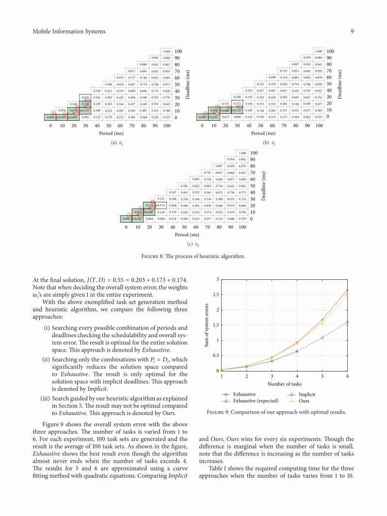
Figure 8: The process of heuristic algorithm.

At the final solution, 𝐽(𝑇,𝐷) = 0.55 = 0.203 + 0.173 + 0.174.Note that when deciding the overall system error, the weights𝑤𝑖’s are simply given 1 in the entire experiment.With the above exemplified task set generation method

and heuristic algorithm, we compare the following threeapproaches:

(i) Searching every possible combination of periods anddeadlines checking the schedulability and overall sys-tem error. The result is optimal for the entire solutionspace. This approach is denoted by Exhaustive.

(ii) Searching only the combinations with 𝑃𝑖= 𝐷𝑖, which

significantly reduces the solution space comparedto Exhaustive. The result is only optimal for thesolution space with implicit deadlines. This approachis denoted by Implicit.

(iii) Search guided by our heuristic algorithm as explainedin Section 5.The result may not be optimal comparedto Exhaustive. This approach is denoted by Ours.

Figure 9 shows the overall system error with the abovethree approaches. The number of tasks is varied from 1 to6. For each experiment, 100 task sets are generated and theresult is the average of 100 task sets. As shown in the figure,Exhaustive shows the best result even though the algorithmalmost never ends when the number of tasks exceeds 4.The results for 5 and 6 are approximated using a curvefitting method with quadratic equations. Comparing Implicit

Number of tasks

0

0.5

1

1.5

2

3

2.5

Sum

of s

yste

m er

rors

Exhaustive ImplicitOurs

1 2 3 4 5 6

Exhaustive (expected)

Figure 9: Comparison of our approach with optimal results.

and Ours, Ours wins for every six experiments. Though thedifference is marginal when the number of tasks is small,note that the difference is increasing as the number of tasksincreases.

Table 1 shows the required computing time for the threeapproaches when the number of tasks varies from 1 to 10.


Table 1: The required computing times for the three approacheswith varying number of tasks.

Number of tasks Exhaustive Implicit Ours1 0.6835ms 0.7885ms 0.69ms2 13.684ms 0.926ms 0.88ms3 1305ms 6ms 0.75ms4 2min 72ms 0.74ms5 (3 hours) 986ms 1.65ms6 (12 days) 1100ms 2.44ms7 (1228 days) (2min) 16.19ms8 (3 years) (26min) 121ms9 (30577 years) (5 hours) 609ms10 (290635 years) (2 days) 1121ms

The numbers in parenthesis are estimated values whereasthe other numbers are actually measured. From the table,Exhaustive requires more than a year when the numberof tasks is only 7. Even for Implicit, when the number oftasks is 10, which is relatively small in practice, the requiredcomputing time exceeds 2 days. Therefore, we can concludethat both Exhaustive and Implicit cannot be used as practicalsize task sets whereas Ours finds solutions even with largertask sets.

In order to prove that our heuristic algorithm producesa high-quality solution compared to other methods, wealso compare Ours with the following two other heuristicalgorithms:

(i) At each iteration, the approach chooses the movingdirection with the higher slope of 𝐽(𝑇

𝑖, 𝐷𝑖). This

approach is denoted by Higher.(ii) At each iteration, the approach chooses the moving

direction with the lower slope of 𝐽(𝑇𝑖, 𝐷𝑖). This

approach is denoted by Lower.

Note that Ours is an extension of Lower, which additionallyconsiders the resulting schedulability as well as the slopewhen deciding the moving direction.

Figure 10 compares the performance of Ours with Higherand Lower. The result is the average of 100 synthesized tasksets for each number of tasks from 1 to 6. As shown in thefigure, Ours shows the best result compared to Higher andLower. By comparingHigher and Lower, Lower shows a betterresult compared toHigher.The result first explains that takingthe lower slope produces a better result than taking the higherslope. Meanwhile, Ours further enhances the performanceby taking the schedulability into consideration as well as theslope at each iteration.

7. Conclusion

By exploiting the trade-off relation of task periods anddeadlines, this paper proposes a novel task set synthesisalgorithm for maximizing the overall system performance.For conducting a measurement study regarding the controlperformance, a simulation environment is developed, whichcan easily gather the performance variations of automotive

Number of tasks

0

0.5

1

1.5

2

2.5

3

Sum

of s

yste

m er

rors

1 2 3 4 5 6

HigherLowerOurs

Figure 10: Comparison of our approach with other heuristicmethods.

control applications while applying various task periods anddeadlines. Starting from the measured data, which confirmsthe trade-off relation, our problem is formally defined asa period and deadline selection problem. The input to ourproblem is each task’s WCET and its measured control per-formance matrix with various periods and deadlines. For thescheduling, DMfixed-priority scheduling is assumed. Since itbecomes quickly intractable to find the optimal solution witheven relatively small number of tasks, this paper proposes aheuristic algorithmwith a linear complexity that finds a high-quality suboptimal solution. Our heuristic algorithm is basedon a gradient descent method with its initial solution at thesmallest period and deadline for each task. Starting from theinitial solution, our algorithm iteratively increases period ordeadline one at a time until the task set is schedulable. Foreach iteration, the task and its moving direction are chosencomparing the control performance reductions.

In our future work, we consider a new system con-figuration where multiple implicit deadline periodic taskscollectively control a single plant. For such systems, a chain oftasks actually controls a plant from sensing to actuation. Bycontrolling each task’s sampling period, we have to indirectlycontrol the sampling frequency and input-output delay theplant actually experiences.

Competing Interests

The authors declare that there are no competing interestsregarding the publication of this paper.

References

[1] K.-E. Arzen, A. Cervin, J. Eker, and L. Sha, “An introductionto control and scheduling co-design,” in Proceedings of the 39thIEEE Confernce on Decision and Control, pp. 4865–4870, IEEE,December 2000.


[2] F. Xia and Y. Sun, “Control-scheduling codesign: a perspectiveon integrated control and computing,”Dynamics of Continuous,Discrete and Impulsive Systems—Series B, vol. 13, supplement 1,pp. 1352–1358, 2006.

[3] A. Cervin and J. Eker, “Control-scheduling codesign of real-time systems: the control server approach,” Journal of EmbeddedComputing, vol. 1, no. 2, pp. 209–224, 2005.

[4] F. Xia and Y.-X. Sun, Control and Scheduling Codesign: FlexibleResource Management in Real-Time Control Systems, SpringerScience & Business Media, 2008.

[5] A. Cervin, D. Henriksson, B. Lincoln, J. Eker, and K.-E. Arzen,“How does control timing affect performance? Analysis andsimulation of timing using jitterbug and truetime,” IEEEControlSystems, vol. 23, no. 3, pp. 16–30, 2003.

[6] Y.Wu, G. Buttazzo, E. Bini, and A. Cervin, “Parameter selectionfor real-time controllers in resource-constrained systems,” IEEETransactions on Industrial Informatics, vol. 6, no. 4, pp. 610–620,2010.

[7] D. Seto, J. P. Lehoczky, L. Sha, and K. G. Shin, “On task schedu-lability in real-time control systems,” in Proceedings of the 199617th IEEE Real-Time Systems Symposium (RTSS ’96), pp. 13–21,December 1996.

[8] D. Seto, J. P. Lehoczky, and L. Sha, “Task period selection andschedulability in real-time systems,” in Proceedings of the 19thIEEE Real-Time Systems Symposium (RTSS ’98), pp. 188–198,December 1998.

[9] E. Bini and M. Di Natale, “Optimal task rate selection in fixedpriority systems,” in Proceedings of the 26th IEEE Real-TimeSystems Symposium (RTSS ’05), 409, 399 pages, December 2005.

[10] E. Bini and A. Cervin, “Delay-aware period assignment incontrol systems,” in Proceedings of the Real-Time Systems Sym-posium (RTSS ’08), pp. 291–300, December 2008.

[11] L. Tan, C. Du, and Y. Dong, “Control-performance-drivenperiod and deadline selection for cyber-physical systems,” inProceedings of the 10th Asian Control Conference (ASCC ’15), pp.1–6, Kota Kinabalu, Malaysia, May 2015.

[12] C.Du, L. Tan, andY.Dong, “Period selection for integrated con-troller tasks in cyber-physical systems,” Chinese Journal ofAeronautics, vol. 28, no. 3, pp. 894–902, 2015.

[13] G. Buttazzo, M. Velasco, and P.Marti, “Quality-of-control man-agement in overloaded real-time systems,” IEEETransactions onComputers, vol. 56, no. 2, pp. 253–266, 2007.

[14] H.-J. Cha, S.-W. Park,W.-H. Jeong, and J.-C. Kim, “Performancetradeoff between control period and delay: lane keeping assistsystem case study,” Journal of the Korea Society of Computer andInformation, vol. 20, no. 11, pp. 39–46, 2015.

[15] B. Lincoln and A. Cervin, “Jitterbug: a tool for analysis ofreal-time control performance,” in Proceedings of the 41st IEEEConference on Decision and Control, vol. 2, pp. 1319–1324, IEEE,Las Vegas, Nev, USA, December 2002.

[16] D. Henriksson, A. Cervin, M. Andersson, and K.-E. Arzen,“Truetime: simulation of networked computer control systems,”in Proceedings of the 2nd IFAC Conference on Analysis andDesign of Hybrid Systems, Alghero, Italy, June 2006.

[17] N. Audsley, A. Burns, M. Richardson, K. Tindell, and A. Wel-lings, “Applying new scheduling theory to static priority pre-emptive scheduling,” Software Engineering Journal, vol. 8, no. 5,pp. 284–292, 1993.

[18] EVIDENCE, “Erika enterprise manual,” http://erika.tuxfamily.org/drupal/.

[19] B. Wymann, “Torcs manual installation and robot tutorial,”http://www.berniw.org/aboutme/publications/torcs.pdf.

[20] Infineon, “Tc1797 user’s manual,” http://www.infineon.com/cms/en/product/.

[21] Tc1796 user’s manual, http://www.infineon.com/cms/en/prod-uct/.

[22] National Instruments, Labview user manual, http://www.ni.com/labview/ko/.

[23] PEAK-System, “Pcan-basic parameters description,” http://www.peak-system.com/PCAN-USB.199.0.html?&L=1.

[24] Logitech, Logitech g25 user manual, http://support.logitech.com/enau/product/g25-racing-wheel.

Submit your manuscripts athttp://www.hindawi.com

Computer Games Technology

International Journal of

Hindawi Publishing Corporationhttp://www.hindawi.com Volume 2014


Distributed Sensor Networks


Advances in

FuzzySystems

Hindawi Publishing Corporationhttp://www.hindawi.com

Volume 2014


ReconfigurableComputing

Hindawi Publishing Corporation http://www.hindawi.com Volume 2014


Applied Computational Intelligence and Soft Computing

Advances in

Artificial Intelligence


Advances inSoftware EngineeringHindawi Publishing Corporationhttp://www.hindawi.com Volume 2014


Electrical and Computer Engineering

Journal of

Journal of

Computer Networks and Communications


Hindawi Publishing Corporation

http://www.hindawi.com Volume 2014

Advances in

Multimedia


Biomedical Imaging


ArtificialNeural Systems

Advances in


RoboticsJournal of



Computational Intelligence and Neuroscience

Industrial EngineeringJournal of


Modelling & Simulation in EngineeringHindawi Publishing Corporation http://www.hindawi.com Volume 2014

The Scientific World JournalHindawi Publishing Corporation http://www.hindawi.com Volume 2014


Human-ComputerInteraction

Advances in

Computer EngineeringAdvances in


Research Article Control-Scheduling Codesign...

Documents

Transcript of Research Article Control-Scheduling Codesign...