Research Article Comparison of Geostatistical Kriging ...
12
Research Article Comparison of Geostatistical Kriging Algorithms for Intertidal Surface Sediment Facies Mapping with Grain Size Data No-Wook Park 1 and Dong-Ho Jang 2 1 Department of Geoinformatic Engineering, Inha University, Incheon 402-751, Republic of Korea 2 Department of Geography, Kongju National University, Kongju 314-701, Republic of Korea Correspondence should be addressed to No-Wook Park; [email protected] Received 13 October 2013; Accepted 8 January 2014; Published 13 February 2014 Academic Editors: Z. Dai and N. Hirao Copyright © 2014 N.-W. Park and D.-H. Jang. is is an open access article distributed under the Creative Commons Attribution License, which permits unrestricted use, distribution, and reproduction in any medium, provided the original work is properly cited. is paper compares the predictive performance of different geostatistical kriging algorithms for intertidal surface sediment facies mapping using grain size data. Indicator kriging, which maps facies types from conditional probabilities of predefined facies types, is first considered. In the second approach, grain size fractions are first predicted using cokriging and the facies types are then mapped. As grain size fractions are compositional data, their characteristics should be considered during spatial prediction. For efficient prediction of compositional data, additive log-ratio transformation is applied before cokriging analysis. e predictive performance of cokriging of the transformed variables is compared with that of cokriging of raw fractions in terms of both prediction errors of fractions and facies mapping accuracy. From a case study of the Baramarae tidal flat, Korea, the mapping method based on cokriging of log-ratio transformation of fractions outperformed the one based on cokriging of untransformed fractions in the prediction of fractions and produced the best facies mapping accuracy. Indicator kriging that could not account for the variation of fractions within each facies type showed the worst mapping accuracy. ese case study results indicate that the proper processing of grain size fractions as compositional data is important for reliable facies mapping. 1. Introduction As transition zones where the land and sea meet, tidal flats are highly productive zones with specific ecosystems. Especially, sediment properties in tidal flats, such as grain size and sediment facies, are related to sediment transport and stability and affect intertidal habitats [1, 2]. ese properties can therefore be useful information sources for effective coastal zone management. e characteristics of intertidal surface sediments are usually described using grain size data. To map sediment grain size distributions, surface sediment samples are first collected via field survey and the information on grain size is then generated through laboratory experiments. From the grain size data, the sediment fractions, as denoted by percentages of sand, silt, and clay, are generally obtained and sedimentary facies are then classified by applying a certain classification scheme, such as Shepard’s rule [3]. Due to the short exposure time of intertidal surfaces and the limitations of sampling cost, however, only limited numbers of field samples are generally available. us, spatial prediction or interpolation is usually applied to generate exhaustive infor- mation over the study area. Many interpolation algorithms ranging from deterministic models (e.g., inverse distance weighting) to geostatistical kriging can be applied to this spa- tial prediction task. Especially, kriging, which can be regarded as a main part of geostatistics, has several advantages over the deterministic models. It can not only account for spatial patterns inherent to sample data such as spatial correlation and anisotropy, but also integrate various types of spatial data such as categorical and/or continuous data [4, 5]. Some kriging algorithms can be applied to intertidal surface sediment facies mapping using grain size data. e first possible approach is indicator kriging that can be applied Hindawi Publishing Corporation e Scientific World Journal Volume 2014, Article ID 145824, 11 pages http://dx.doi.org/10.1155/2014/145824
Transcript of Research Article Comparison of Geostatistical Kriging ...

Research ArticleComparison of Geostatistical Kriging Algorithms forIntertidal Surface Sediment Facies Mapping with GrainSize Data
No-Wook Park1 and Dong-Ho Jang2
1 Department of Geoinformatic Engineering Inha University Incheon 402-751 Republic of Korea2Department of Geography Kongju National University Kongju 314-701 Republic of Korea
Correspondence should be addressed to No-Wook Park nwparkinhaackr
Received 13 October 2013 Accepted 8 January 2014 Published 13 February 2014
Academic Editors Z Dai and N Hirao
Copyright copy 2014 N-W Park and D-H Jang This is an open access article distributed under the Creative Commons AttributionLicense which permits unrestricted use distribution and reproduction in any medium provided the original work is properlycited
This paper compares the predictive performance of different geostatistical kriging algorithms for intertidal surface sediment faciesmapping using grain size data Indicator kriging whichmaps facies types from conditional probabilities of predefined facies types isfirst considered In the second approach grain size fractions are first predicted using cokriging and the facies types are thenmappedAs grain size fractions are compositional data their characteristics should be considered during spatial prediction For efficientprediction of compositional data additive log-ratio transformation is applied before cokriging analysisThe predictive performanceof cokriging of the transformed variables is compared with that of cokriging of raw fractions in terms of both prediction errors offractions and faciesmapping accuracy From a case study of the Baramarae tidal flat Korea themappingmethod based on cokrigingof log-ratio transformation of fractions outperformed the one based on cokriging of untransformed fractions in the prediction offractions and produced the best facies mapping accuracy Indicator kriging that could not account for the variation of fractionswithin each facies type showed the worst mapping accuracy These case study results indicate that the proper processing of grainsize fractions as compositional data is important for reliable facies mapping
1 Introduction
As transition zones where the land and sea meet tidalflats are highly productive zones with specific ecosystemsEspecially sediment properties in tidal flats such as grain sizeand sediment facies are related to sediment transport andstability and affect intertidal habitats [1 2] These propertiescan therefore be useful information sources for effectivecoastal zone management
The characteristics of intertidal surface sediments areusually described using grain size data To map sedimentgrain size distributions surface sediment samples are firstcollected via field survey and the information on grain sizeis then generated through laboratory experiments Fromthe grain size data the sediment fractions as denoted bypercentages of sand silt and clay are generally obtained andsedimentary facies are then classified by applying a certain
classification scheme such as Shepardrsquos rule [3] Due to theshort exposure time of intertidal surfaces and the limitationsof sampling cost however only limited numbers of fieldsamples are generally available Thus spatial prediction orinterpolation is usually applied to generate exhaustive infor-mation over the study area Many interpolation algorithmsranging from deterministic models (eg inverse distanceweighting) to geostatistical kriging can be applied to this spa-tial prediction task Especially krigingwhich can be regardedas a main part of geostatistics has several advantages overthe deterministic models It can not only account for spatialpatterns inherent to sample data such as spatial correlationand anisotropy but also integrate various types of spatial datasuch as categorical andor continuous data [4 5]
Some kriging algorithms can be applied to intertidalsurface sediment facies mapping using grain size data Thefirst possible approach is indicator kriging that can be applied
Hindawi Publishing Corporatione Scientific World JournalVolume 2014 Article ID 145824 11 pageshttpdxdoiorg1011552014145824
2 The Scientific World Journal
directly to categorical data [6] because the target attributefor intertidal surface sediment facies mapping is categoricalinformation In this approach sample data are first classifiedas sediment facies according to their grain size fractionsand indicator transform is then applied Spatial correlationinformation of indicator-coded binary data for each sedimentclass is used for indicator kriging
As another approach grain size fractions are first pre-dicted at unsampled locations and the classification rule isfinally applied to map sediment facies over the study areaSpatial correlation information is directly derived from eachgrain size component and used for the kriging algorithmDuring spatial prediction of each grain component howeverspecial care should be taken due to the particular characteris-tics of the grain size fractionsThe grain size fractions whichare usually expressed as the relative proportions are regardedas compositional data that have both nonnegative values anda constant sum (eg 1 or 100) [7] Due to these constraintsspurious correlation is observed in compositional data suchthat as one component decreases one or more of the othercomponents should increase and vice versa Although spatialauto- and cross-correlation information can be explained incokriging the direct application of conventional cokrigingwithout consideration for these constraints may generatenegative values and the sum of predicted component valuesmay not be constant For appropriate consideration of thecharacteristics of compositional data in spatial predictionlog-ratio based transformation is usually applied to theoriginal compositional data prior to kriging analysis [8]
The spatial prediction of grain size fractions is not afinal goal per se but it should be regarded as a preliminarystep toward intertidal sediment facies mapping Log-ratiotransformation is much more appropriate for compositionaldata analysis However prediction results are still subject toerrors attached to the prediction and those errors may affectthe subsequent facies mapping results because predictionresults are directly fed into the classification rule Thus thepotential of the application of log-ratio transformation tospatial prediction of grain size fractions should be evaluatedin terms of not only prediction accuracy of grain sizefractions but also facies mapping accuracy
In relation to spatial prediction of compositional dataand subsequent classification several studies have beencarried out for soil texture classes mapping [9 10] seabedsediment texture classes mapping [11] and soil erodibilityfactor mapping [12] These studies reported that if the specialrequirements of compositional data are not considered spa-tial prediction of both fractions and classes will not generatereliable mapping results To our knowledge however spatialprediction of sediment fractions as compositional data andthe comparison with indicator kriging have not yet beenconducted for intertidal surface sediment facies mapping
The objective of this paper is to evaluate the predic-tive performance of the following three different krigingapproaches for intertidal surface sediment faciesmapping (1)indicator kriging (2) cokriging without data transformationand (3) cokrigingwith additive log-ratio (alr) transformationThis performance evaluation is illustrated through a case
Korea
Study area
Anmyeondo
Halmi isle
Figure 1 Location of the case study area Black dots denote samplingsites
study with a grain size data set acquired in the Baramaraetidal flat Korea
2 Study Area and Data
The application of different kriging algorithms for surfacesediment facies mapping is compared via a case study inthe Baramarae tidal flat Korea The study area is underlainby Precambrian metasediment the Kyeonggi MetamorphicComplex and several intrusive rocks [13] In the studyarea two sea stacks including the Halmi and Seomot isleswave-cut platform and sand dunes have developed andblocked ocean waves so large tidal flats have developed at anindentation in the coast The west coastal areas face the opensea and are directly affected by ocean waves so sand spitsbeach and coastal sanddunes have developed [1]Meanwhilemuch sediment has been continuously provided by the tidalcurrents in the eastern part of the coast so large tidal flatswere developed The tides in the study area are semidiurnalwith a mean tidal range of 46m The mean tidal currentvelocities near the study area are 08msec and 09msecduring flow tide and ebb tide respectively [14]
In the study area a field survey was conducted in Febru-ary 2009 and 174 surface sediment samples were collected(Figure 1) A portable GPS (GARMIN 60CSx) was used forpositioning of the sample locations The sediment sampleswere sieved using a set of sieves and then analyzed using aMastersizer 2000 at the laboratory to obtain sample fractionssuch as relative percentages of sand silt and clay Detailedprocedures for sample data processing at the laboratory canbe found in Jang et al [14]
3 Methods
Kriging which is a generalized least-squares interpolationmethod predicts attribute values at unsampled locations byusing neighboring samples and spatial correlation informa-tion modeled by variogram [5 15]
Suppose that there are 119899 sediment samples with 119863
components 119911119894(u120572) 120572 = 1 119899 119894 = 1 119863 in the
study area Each sample is a composition with 119863 = 3
components which are the percentages of sand silt and
The Scientific World Journal 3
clay In this case study the following three different krigingalgorithms are compared and evaluated indicator krigingcokriging without data transformation and cokriging withalr transformation
31 Indicator Kriging of Facies Types The first krigingapproach considered in this study is indicator kriging thatattempts to model probabilities for all categories by consid-ering neighboring indicator-coded values [6] The indicatorapproach requires a preliminary coding of sample data intolocal prior probabilities By directly applying the classificationrule sediment facies types are first identified at each samplelocation According to the percentage of sand each sampleis classified into the following three facies types sand flats(above 70) mixed flats (30ndash70) and mud flats (0ndash30)after Folk [16] Suppose that 120596
119896 119896 = 1 2 3 is a set of the
above three sediment facies types Then the sediment faciestype at sample locations (120596(u
120572)) is coded into three binary
indicator probabilities (119868(u120572 120596119896)) as follows
119868 (u120572 120596119896) =
1 if 120596 (u120572) = 120596119896
0 otherwise
119896 = 1 2 3
(1)
The binary indicator variable is interpreted as the prob-ability for a certain sediment facies type to prevail at aparticular location the probability is 1 if it prevails and 0if it does not After indicator coding variogram modelingfor each of the three indicator variables is conducted toincorporate spatial correlation information into the indicatorkriging system
The conditional probability 119901(u 120596119896) at any location is
regarded as the conditional expectation of the indicatorrandom function 119868(u 120596
119896) In this paper it is estimated by
ordinary kriging using neighboring indicator data
119901lowast(u 120596119896) = 119868lowast(u 120596119896) =
119898
sum120572=1
120582120572(u 120596119896) 119868 (u120572 120596119896)
with119898
sum120572=1
120582120572(u 120596119896) = 1 119896 = 1 2 3
(2)
where m is the number of neighboring samples within apredefined search neighborhood and 120582
120572(u 119896) is an ordinary
kriging weight assigned to the neighboring indicator valuesat a prediction location u
The ordinary kriging weight is calculated by solving thefollowing ordinary kriging system [5]119898
sum120573=1
120582120573(u 120596119896) 119862119868(u120572minus u120573 120596119896) + 120583 (u 120596
119896)
= 119862119868(u120572minus u 120596
119896) 120572 = 1 119898 119896 = 1 2 3
119898
sum120572=1
120582120572(u 120596119896) = 1
(3)
where 120583(u 119896) is the Lagrange parameter for meeting theconstraint on the weights such that the sum of the kriging
weights is 1119862119868(u120572minusu120573 120596119896) and119862
119868(u120572minusu 120596119896) are the data-to-
data covariance and the data-to-sample indicator covariancefor each facies type 120596
119896 respectively
Kriging is a nonconvex interpolator and indicator krigingis independently and repeatedly applied to the set of K faciestypes Thus the estimated probability may be outside theinterval [0 1] and the constant sum constraint may not besatisfied [17] This order relation violation is corrected byresetting any probability outside the interval to the closestbound 0 or 1 and standardization
After estimating the conditional probability at unsampledlocations the final sediment facies types over the study areaare mapped by applying the maximum a posteriori rulein a way that the facies type with the largest conditionalprobability is allocated
32 Cokriging of Fractions In this approach the fractions arefirst predicted and the sediment facies type is then classifiedaccording to sand content as in the indicator approachThe kriging algorithm applied in this approach is cokrigingwhich can integrate multiple correlated variables In thisstudy two cokriging algorithms with different input fractionsare applied to compare the cases of with and without datatransformation for compositional data
First conventional cokriging is directly applied to theoriginal fractions of sand silt and clay components Thefractions are estimated via cokriging by accounting forboth spatial auto- and cross-correlation information Theordinary cokriging for estimation of the ith fraction valuesat unsampled location is written as
119911lowast
119894(u) =
119898
sum120572=1
120582120572 (u) 119911119894 (u120572)
+
119863
sum119895=2
119898
sum120572119895=1
120582120572119895(u) 119911119895 (u120572) 119895 = 1 119863
119898
sum120572=1
120582120572 (u) = 1
119898
sum120572119895=1
120582120572119895(u) = 0 119895 = 2 119863
(4)
To compute the ordinary cokriging weight 120582120572119895
given tothe jth component at the 120572th sample location the direct andcross-covariance functions (equivalently variograms) shouldbe inferred For two variables 119911
119894and 119911
119895 cross-variogram
which is a quantitative measure of spatial variability betweentwo variables is defined as
120574119894119895 (h) =
1
2119873 (h)
times
119898
sum120572=1
[119911119894 (u) minus 119911
119894 (u + h)] [119911119895 (u) minus 119911119895 (u + h)]
(5)
4 The Scientific World Journal
where 119873(h) is the number of data pairs separated by a lagdistance h
All direct and cross-variograms are inferred by a linearmodel of coregionalization (LMC) which is the way to jointlymodel them [5] After generating cokriging estimates for allfractions the same classification rule by sand content is alsoapplied and the sediment facies types are finally obtained overthe study area
As mentioned in Section 1 the direct application ofcokriging to original fractions has several drawbacks As frac-tions are bounded in a simplex space the cokriging estimatesmay have unrealistic negative values and do not satisfy theconstant sum constraint To solve this problem arising fromthe nature of compositional data the second approach iscokriging of alr transformed fractions By applying the alrtransformation before cokriging analysis grain size fractionsin the simplex space become unbounded negative or positivevalues which allows standard cokriging to be applied
In this study the three components of surface sedimentsat sample locations are transformed to their alr values asfollows
alr119894(u120572) = ln[
119911119894(u120572)
119911119863(u120572)] 119894 = 1 119863 minus 1 (6)
where 119911119863
is the arbitrarily chosen denominator of thetransformation
After alr transformation119863 minus 1 transformed variables (inour case 2 variables) are generated and cokriging is appliedto these variables For cokriging analysis all direct and cross-variograms are inferred from the transformed variables notfrom the original fraction values The cokriging estimatesalrlowast119894(u) for119863minus1 transformed variables are back-transformed
by taking the additive logistic transformation to ensure theconstraints of compositional data as follows
119911lowast
119894(u) =
exp (alrlowast119894)
1 + sum119863minus1
119894=1exp (alrlowast
119894)
119894 = 1 119863 minus 1
119911lowast
119863(u) = 1
1 + sum119863minus1
119894=1exp (alrlowast
119895)
(7)
Finally the classification rule is applied to the cokrigingestimates in (7) to map the surface sediment facies types
33 Performance Evaluation In the case of indicator krigingof facies types the final output is the facies type at all locationsin the study area On the other hand cokriging of fractionsregardless of the application of alr transformation generatestwo outputs one for the fraction of each component andthe other for the facies type In this study the predictionperformance of both fractions and facies types is evaluatedvia leave-one-out cross-validation One sample location istemporarily eliminated from the data sets and any krigingalgorithms with the remaining samples are applied to predicteither the fraction value or the facies type at the eliminatedlocation This procedure is repeated for all sample locations
Two different evaluation criteria for the prediction offractions and facies types are applied in this paper The
predictive performance of fractions especially for the effectsof alr transformation before cokriging is quantified using themean absolute error (MAE) for each component defined as
MAE119894=1
119899
119899
sum120572=1
1003816100381610038161003816119911lowast
119894(119906120572) minus 119911119894(119906120572)1003816100381610038161003816 119894 = 1 2 3 (8)
The relative improvement index (RI) is also computed toquantify the effects on prediction capability of alr transfor-mation before cokriging as
RI119894= 100 sdot
[MAEalr119894minusMAEwithout alr
119894]
MAEwithout alr119894
119894 = 1 2 3 (9)
where MAEalr119894
and MAEwithout alr119894
denote the MAE values forcokriging with and without alr transformation respectively
As the facies type is a categorical attribute differentevaluation criteria are applied for comparisons of faciesmapping accuracy First a confusion matrix is first preparedand related accuracy statistics including overall accuracyclass-wise accuracy and kappa coefficient are calculated bycomparing the true facies type and the predicted type at eachsample location The overall accuracy is the percentage ofcorrectly classified locations in all samples and the class-wise accuracy is a measure of the probability that a predictedsample actually represents the facies type on the true sampleThe kappa coefficient is a measure of the difference betweenthe actual agreement and the change agreement [18]
4 Results and Discussion
41 Exploratory Data Analysis Prior to geostatistical anal-ysis the descriptive statistics of the grain size fractions at174 surface sediments were computed and are summarizedin Table 1 The median values for sand silt and clay were6039 3643 and 308 respectively which indicates thatthe majority of samples consist of coarse-grained particlesThe portions for sand mixed and mud flats at sample loca-tions were 391 414 and 195 respectively (Figure 2) Asexpected from the low clay content the portion of mud flatswas relatively small Zero values in silt and clay componentswere observed among about 16 and 19 of all samplesrespectively The alr transformation is not defined if anyobserved fraction value is zero so the zero values shouldbe replaced by reasonable nonzero values By following thenonparametric multiplicative strategy of Martın-Fernandezet al [19] each rounded zero in the composition was replacedby an appropriate small value and the nonzero values werethen renormalized to ensure no zero values and the constantsum constraint The small value for replacement was set to01 which was half the smallest nonzero value in the claycomponentThese renormalized fractionswere used as inputsfor the subsequent geostatistical analysis
42 Indicator Kriging Results Before indicator kriging threebinary indicator variables were first generated at samplelocations by considering the three sediment facies typesThen experimental indicator variograms for the three indi-cator variables were computed and variogram modeling was
The Scientific World Journal 5
Table 1 Summary statistics of grain size fractions in all samples
Statistic ComponentSand Silt Clay
Mean 5914 3723 363Standard deviation 3042 2748 317Minimum 035 000 00025 quantile 3641 1254 083Median 6039 3643 30875 quantile 8686 5844 578Maximum 10000 9235 1393Skewness minus016 014 068Portion of zero values () 000 1609 1897
Table 2 Parameters for indicator variogram models
Facies type Model Nugget Partial sill Range (m)Sand flats Exponential 0103 0223 3015Mixed flats Spherical 0186 0065 1029Mud flats Spherical 0099 0295 7575
finally implemented None of the indicator variables showedsignificant anisotropy so the omnidirectional variogramswere computed and modeled The parameters of the vari-ogram models are listed in Table 2 Especially the indicatorvariogram of mixed flats was modeled with very high nuggeteffects and a relatively shorter range (about 13 km) Ordinaryindicator kriging was implemented using GSLIB [17] and theorder relation violation was also corrected
The conditional probabilities for the three facies typeswere generated on a 4m by 4m grid and are given in Figure 3Sand dunes near Halmi isle and tidal channels which are notdirectly related to intertidal surface sediments were maskedout and excluded for kriging analysis The relatively shorterrange values of the indicator variogram models led to abullrsquos-eye effect around the sample locations However theoverall patterns of the conditional probability for each faciestype could be observed The conditional probability for sandflats was much higher in the southwest and northeast partsof Halmi isle Mixed flats prevailed around the large tidalchannels and showed a strong bullrsquos-eye effect due to therelatively shorter range Both the east seaward side and thenorthwest and northeast parts of the inner bay showed arelatively high probability for mud flats
The final surface sediment facies types were mapped byapplying the maximum a posteriori rule to the conditionalprobabilities and are shown in Figure 4 As expected from theconditional probabilities for the three facies types in Figure 3sand flats are widely located at the front and back sides ofHalmi isle Mixed flats are located along the tidal channelsand also at the inner bay areas Mud flats occupy relativelysmall local areas in the northwest of the inner bay and theeast seaward side of the study area The mapping result alsoshowed some spot areas such as mud flats near the tidalchannels and sand flats in the southeast area These isolatedsmall areas are mainly located near some samples showing
Silt0 10 20 30 40 50 60 70 80 90 100
Sand
0
10
20
30
40
50
60
70
80
90
100
Clay
010
20
30
40
50
60
70
80
90
100
Sand flat
Mixed flat
Mud flat
Figure 2 Ternary diagrams of three grain size components andsediment facies classes
the intermingled patterns of conditional probabilities frommixed flats and mud flats
43 Cokriging Results For cokriging of the original frac-tions without alr transformation three direct and twocross-variograms were modeled using the LMC No stronganisotropywas observed so the omnidirectionalmodels werefitted and the parameters for the fitted models are listed inTable 3 From the variogram models and correlation coeffi-cients the sand component had a strong negative correlationwith the silt and clay components which indicated that as thesand component increases the other components decreaseThe silt and clay components had a positive correlation witheach other These correlation patterns are typical character-istics of compositional data so called spurious correlation[7 8]
To investigate the effects of considerations on the natureof compositional data the alr transformation was appliedto raw fractions using (6) The denominator 119911
119863in (6) was
experimentally set to the sand component In (6) 1199111and 119911
2
were also set to the silt and clay components respectivelySo two new alr transformed variables (ie alr
1and alr
2)
were generated and they were used as inputs for cokrigingTwo direct and one cross-variograms were also modeledusing the LMC The LMC was fitted using nugget effectsand an exponential model (Table 4) Although the same twobasic structures were fitted for both original fractions andalr transformed variables alr transformation led to a longerpractical range of the exponential model
Cokriging was undertaken by using (4) and all variogrammodels After generating cokriging estimates of the two alrtransformed variables the inverse log-ratio transformationwas applied by using (7) to generate the grain size fractionsin an original simplex space Especially the sums of thethree fraction values at all grids were computed to examineif the direct application of cokriging to original fractionssatisfied the constant sum constraint on compositional dataAs shown in Figure 5 the sums were very close to 100
6 The Scientific World Journal
0 05 1025(km)
126∘2299840030998400998400E 0998400998400E126 ∘23998400 126∘2399840030998400998400E 126∘2499840030998400998400E0998400998400E126 ∘2499840036
∘25
998400 0998400998400N
0998400998400N
36∘24
998400 40998400998400
N36
∘24
998400 2
09-1008-0907-0806-07
05-06
04-05
03-04
02-03
01-0200-01
(a)
0 05 1025(km)
126∘2299840030998400998400E 0998400998400E126 ∘23998400 126∘2399840030998400998400E 126∘2499840030998400998400E0998400998400E126 ∘24998400
36∘25
998400 0998400998400N
0998400998400N
36∘24
998400 40998400998400
N36
∘24
998400 2
09-1008-0907-0806-07
05-06
04-05
03-04
02-03
01-0200-01
(b)
0 05 1025(km)
126∘2299840030998400998400E 0998400998400E126 ∘23998400 126∘2399840030998400998400E 126∘2499840030998400998400E0998400998400E126 ∘24998400
36∘25
998400 0998400998400N
0998400998400N
36∘24
998400 40998400998400
N36
∘24
998400 2
09-1008-0907-0806-07
05-06
04-05
03-04
02-03
01-0200-01
(c)
Figure 3 Conditional probability of each facies type prevailing over the study area by indicator kriging (a) sand flats (b) mixed flats and(c) mud flats
but the constant sum constraint was not satisfied at alllocations In addition some negative values were observedat some locations especially in the clay component whichhad relatively small values The values at any locations wherenegative values were estimated andor the sum was not 100were modified to ensure the characteristics of compositionaldata in such a way that negative values or those greater than100 were reset to 0 or 100 respectively Normalizationwas then applied to ensure the constant sum constraintThis modification procedure as postprocessing may result insome distortions or bias thus leading to a misclassification ofsediment facies types On the contrary the application of alrtransformation before cokriging analysis perfectly satisfiedthe constraints of compositional data
The cokriging estimates for sand silt and clay compo-nents without and with alr transformation are shown in
Figures 6 and 7 respectively In both cokriging estimatesthe overall patterns of the fractions were similar in such away that areas with high sand content have low content ofsilt and clay and vice versa However some locations showedslightly different values which was attributed to the differentrange values of the variogram models When comparing thesand content in Figures 6(a) and 7(a) cokriging with alrtransformation led to higher and lower values of sand in thenorth or back side of Halmi isle and in the inner bay areasrespectively compared with cokriging estimates without alrtransformation In the silt content estimates by cokrigingwithalr transformation (Figure 7(b)) low and high values weredistributed more widely than in Figure 6(b)The clay contentshowed overall low valueswith high values in the east seawardside The differences between Figures 6(c) and 7(c) for clayare distinct at the north or back side of Halmi isle in which
The Scientific World Journal 7
Sand flatMixed flatMud flat
0 05 1025(km)
126∘2299840030998400998400E 0998400998400E126 ∘23998400 126∘2399840030998400998400E 126∘2499840030998400998400E0998400998400E126 ∘24998400
36∘25
998400 0998400998400N
0998400998400N
36∘24
998400 40998400998400
N36
∘24
998400 2
Figure 4 Surface sediment facies distribution generated by indica-tor kriging
0300
0200
0100
0000
9800 9900 10000 10100 10200
Mean 99996Std dev 0321Coef of var 0003Maximum 101586Upper quartile 100123Median 100014Lower quartile 99858Minimum 98708
Freq
uenc
y
Figure 5 Histogram of the sums of the three fraction values at allgrid locations predicted by cokriging without alr transformation Inthe box plot below the histogram outside whiskers correspond tothe 95 probability intervals inside boxes to the 50 probabilityintervals and vertical lines in the box to the median value
the low content of clay was widely distributed in Figure 7(c)compared to some areas having a relatively high content ofclay in Figure 6(c)
The fractions estimated by cokriging with different inputswere directly used for sediment facies mapping Thus thesedifferent spatial patterns of fractions led to the different map-ping results and also different levels of accuracy Leave-one-out cross-validation was carried out to quantitatively evaluatethe predictive performance of the fraction estimates by thetwo cokriging algorithms In the cross-validation resultsshown in Table 5 cokriging with alr transformation outper-formed cokriging with untransformed raw fractions for allthree componentsThemaximum relative improvement overcokriging of untransformed fractions was about 855 forsand The clay component which was the smallest content
Table 3 Parameters for the fitted linear model of coregionalizationfor original three components
Model Variance-covariance matrix Range (m)
Nugget
Sand Silt Clay
mdashSand 210005Silt minus175013 175022Clay minus17001 16051 2201
Exponential
Sand Silt Clay
1386Sand 697460Silt minus630652 570252Clay minus68990 62292 7684
Table 4 Parameters for the fitted linear model of coregionalizationfor alr
Model Variance-covariance matrix Range (m)
Nuggetalr1 alr2
mdashalr1 1332alr2 0911 1116
Exponentialalr1 alr2
2908alr1 15381alr2 13069 11865
Table 5 Predictive performance of fraction estimates by differentcokriging algorithms
Component MAE RI ()Cokriging withoutalr transformation
Cokriging withalr transformation
Sand 1571 1436 855Silt 1417 1313 734Clay 171 162 527
in the sediments showed the lowest relative improvementThese cross-validation results confirmed that cokriging ofalr transformed data led to reliable fractions mapping overthe study area As the predicted fractions values are directlyused tomap sediment facies types the prediction accuracy offraction values will greatly affect the facies mapping resultsIt should be noted that the facies mapping accuracy dependson the accuracy of all components due to the nature of thecompositional data although sediment facies mapping frompredicted fractions is based only on sand content
The sediment facies distributions based on the twodifferent cokriging algorithms were generated by using thesame classification rule (ie sand content) The mappingresults are presented in Figure 8 As expected from the widedistribution of sand and silt in Figure 7 cokriging with alrtransformation generated the relatively wide distributions ofboth sand flats around Halmi isle and mud flats in the innerbay When compared with the facies distribution generatedby indicator kriging shown in Figure 4 some spots classifiedinto mud flats near the tidal channels in Figure 4 disappearedin both Figures 6 and 7 As kriging is an exact interpolatorit honors data values at sample locations [5] Thus the faciestypes at sample locations are reproduced in all maps by any
8 The Scientific World Journal
0 05 1025(km)
126∘2299840030998400998400E 0998400998400E126 ∘23998400 126∘2399840030998400998400E 126∘2499840030998400998400E0998400998400E126 ∘24998400
36∘25
998400 0998400998400N
0998400998400N
36∘24
998400 40998400998400
N36
∘24
998400 2
90ndash100
80ndash90
70ndash80
60ndash70
50ndash60
40ndash50
30ndash40
20ndash30
10ndash200ndash10
(a)
0 05 1025(km)
126∘2299840030998400998400E 0998400998400E126 ∘23998400 126∘2399840030998400998400E 126∘2499840030998400998400E0998400998400E126 ∘24998400
36∘25
998400 0998400998400N
0998400998400N
36∘24
998400 40998400998400
N36
∘24
998400 2
90ndash100
80ndash90
70ndash80
60ndash70
50ndash60
40ndash50
30ndash40
20ndash30
10ndash200ndash10
(b)
0 05 1025(km)
126∘2299840030998400998400E 0998400998400E126 ∘23998400 126∘2399840030998400998400E 126∘2499840030998400998400E0998400998400E126 ∘24998400
36∘25
998400 0998400998400N
0998400998400N
36∘24
998400 40998400998400
N36
∘24
998400 2
9minus118-97-86-7
5-64-53-42-3
1-20-1
(c)
Figure 6 Spatial distributions of fractions generated by cokriging of original fractions (a) sand (b) silt and (c) clay
kriging algorithms However the use of different mappingprocedures led to the different mapping results near thesample locations In the facies mapping result based onindicator kriging spatial correlation structures of facies typesare directly used in indicator kriging so any locations nearsamples tend to have the same facies type depending on thecorrelation strength Meanwhile the facies mapping schemebased on cokriging of fractions first generated fractionestimates over the study area and the mapping rule was thenapplied as a final stage Thus spatial correlation structures ofthe fraction values are only considered for the mapping offractions and relatively few isolated locations were mapped
The following common or overall patterns of sedimentfacies distributions were observed over the study area inFigures 4 and 8 Sand flats are mainly located near Halmi isleespecially the front or southern areas ofHalmi isle are open tothe outer sea so sediments in these areas have been depositedunder the depositional environments with strong sediment
supply Mixed flats which are located along the large tidalchannels at the east of the study area are affected by bothtidal currents and ocean wavesThemud flats observed at theinner bay were developed by the reversing tidal currents orthe decrease of depositional energy due to the topographiceffects The large sand bar located in the southeastern partof the study area has blocked the wave energy allowing fine-grained sediments to be continuously deposited and mudflats developed at the east seaward side of the study area
44 Mapping Accuracy Assessment Like the comparison ofthe predictive performance of cokriging with different inputdata leave-one-out cross-validation was also implemented toquantitatively assess facies mapping accuracy For indicatorkriging conditional probabilities at a temporarily eliminatedsample locationwere estimated by the remaining sample dataThen the MAP rule was also applied to determine the faciestype at the eliminated location For two cokriging algorithms
The Scientific World Journal 9
0 05 1025(km)
126∘2299840030998400998400E 0998400998400E126 ∘23998400 126∘2399840030998400998400E 126∘2499840030998400998400E0998400998400E126 ∘24998400
36∘25
998400 0998400998400N
0998400998400N
36∘24
998400 40998400998400
N36
∘24
998400 2
90ndash100
80ndash90
70ndash80
60ndash70
50ndash60
40ndash50
30ndash40
20ndash30
10ndash200ndash10
(a)
0 05 1025(km)
126∘2299840030998400998400E 0998400998400E126 ∘23998400 126∘2399840030998400998400E 126∘2499840030998400998400E0998400998400E126 ∘24998400
36∘25
998400 0998400998400N
0998400998400N
36∘24
998400 40998400998400
N36
∘24
998400 2
90ndash100
80ndash90
70ndash80
60ndash70
50ndash60
40ndash50
30ndash40
20ndash30
10ndash200ndash10
(b)
0 05 1025(km)
126∘2299840030998400998400E 0998400998400E126 ∘23998400 126∘2399840030998400998400E 126∘2499840030998400998400E0998400998400E126 ∘24998400
36∘25
998400 0998400998400N
0998400998400N
36∘24
998400 40998400998400
N36
∘24
998400 2
9minus118-97-86-7
5-64-53-42-3
1-20-1
(c)
Figure 7 Spatial distributions of fractions generated by cokriging of alr transformed variables (a) sand (b) silt and (c) clay
fraction values predicted at all sample locations have alreadybeen obtained from leave-one-out cross-validation So thesediment facies types at all sample locations were determinedbased on the cross-validated sand content True facies types atsample locations which are required to construct a confusionmatrix were also determined by applying the same classifica-tion rule
Several statistics were computed from the confusionmatrix as quantitative measures of accuracy assessment andare listed in Table 6 Facies mapping based on cokriging of alrtransformed variables showed the best mapping accuracy interms of both overall accuracy and kappa coefficient whichachieved 75p and 98p increases in overall accuracy com-pared with that from cokriging of untransformed fractionsand that from the indicator kriging approach respectivelyThe indicator approach afforded the worst mapping accuracyThe class-wise accuracy was also the best in the mappingresults from cokriging with alr transformation except for the
mud flats in which cokriging without data transformationshowed slightly better accuracy These evaluation resultsconfirmed the effectiveness of andnecessity for the predictionof fraction values with data transformation as a first stageand the subsequent mapping for sediment facies mappingEspecially the characteristics of compositional data shouldbe considered for spatial prediction of fraction values and theprediction results affected the final facies mapping results
The worst mapping accuracy by the indicator krigingapproach can be explained as follows The indicator krigingapproach requires the predefinition of facies types at samplelocations As shown in the ternary diagram of Figure 2 eachfacies type occupies a certain zone in the ternary diagramso the sediment classified as the same facies type can havevery different sand contents For example two sedimentsamples having a sand content of 31 and 69 respectivelyare classified as the same mixed flats type However thecharacteristics of the former and latter sediments are similar
10 The Scientific World Journal
Sand flatMixed flatMud flat
0 05 1025(km)
126∘2299840030998400998400E 0998400998400E126 ∘23998400 126∘2399840030998400998400E 126∘2499840030998400998400E0998400998400E126 ∘24998400
36∘25
998400 0998400998400N
0998400998400N
36∘24
998400 40998400998400
N36
∘24
998400 2
(a)
Sand flatMixed flatMud flat
0 05 1025(km)
126∘2299840030998400998400E 0998400998400E126 ∘23998400 126∘2399840030998400998400E 126∘2499840030998400998400E0998400998400E126 ∘24998400
36∘25
998400 0998400998400N
0998400998400N
36∘24
998400 40998400998400
N36
∘24
998400 2
(b)
Figure 8 Surface sediment facies distribution generated by cokriging (a) without and (b) with alr transformation
Table 6 Mapping accuracy statistics by different mapping algo-rithms
Statistics Indicatorkriging
Cokrigingwithout alr
transformation
Cokrigingwith alr
transformationOverall accuracy() 6379 6609 7356
Kappa coefficient 042 044 058Class-wiseaccuracy ()
Sand flats 8065 8333 8361Mixed flats 5543 5648 6585Mud flats 5000 7500 7419
to those of mud flats and sand flats respectively Thus usingthe predefined class cannot account for the variation offraction values within each facies type This variation withinthe facies type may result in the confusion between nearbyfacies types within the ternary diagram
Another limitation of the indicator kriging approach isits inability to represent all possible facies types not observedat sample locations In this study the three facies types wereexperimentally predefined and mapped according to sandcontent Other classification ormapping rules can be appliedfor example Shepardrsquos rule [3] These classification rules arebased on the relative proportions among sand silt and clayFor example according to Shepardrsquos classification if the claycontent is less than 20 the sand content is less than 75and is greater than the silt content and the silt contentis greater than the clay content the sediment is classifiedas silty sand When considering this classification rule thesmall number of sediment samples which is a typical case ofdata collection in tidal flats may result in several practicalissues If the above classification rule is applied to very fewsamples some sediment types may not be contained among
the predefined types from the sample data andmay thereforenot exist in the final mapping result although they shouldbe included For the application of indicator kriging it maybe difficult or even impossible to capture spatial patterns andmodel variograms of a certain sediment type in which veryfew samples are classified The mapping method based onthe prediction of fractions before applying any classificationrules can overcome these limitations of the indicator krigingapproach
5 Conclusions
Three different kriging algorithms have been compared andevaluated for intertidal surface sediment facies types A casestudy using grain size samples collected in the Baramaraetidal flat Korea indicated that the prediction of fractionsvalues in advance and the subsequent classification improvedmapping accuracy compared to that from the direct predic-tion of predefined facies types via indicator kriging Thus aprerequisite is to generate reliable predictions of grain sizefractions for facies mappingWhen comparing two cokrigingalgorithms with different variables spatial prediction basedon cokriging of log-ratio transformed variables could satisfyall constraints for compositional data and produce not onlybetter accuracy for the prediction of fractions but alsothe best mapping accuracy when compared with spatialprediction based on cokriging of raw fraction values Thusthe prediction of fraction values which can account forthe characteristics of grain size fractions as compositionaldata should be applied before cokriging analysis to generatereliable facies mapping results
From amethodological point of view themajor finding inthis paper can be further extended to improve facies mappingaccuracy When sparse sediment samples are available as inthe case in tidal flats more densely sampled or exhaustivelysampled auxiliary data which are related to the character-istics of grain size data can improve the prediction quality
The Scientific World Journal 11
Remote sensing data [1 2] or terrain data [20 21] can beeffectively used to improve the prediction of grain size orsediment facies When integrating these auxiliary data withgrain size data however the characteristics of compositionaldata should still be considered Although previous studies[2 20 21] reported the ability of terrain data to complementthe sparse grain size data the proper processing of grainsize data as compositional data was not considered Theintegration of alr transformed fractions with high-resolutionremote sensing data will be considered in future work
Conflict of Interests
The authors declare that there is no conflict of interestsregarding the publication of this paper
Acknowledgments
This work was supported by Basic Science Research Programthrough the National Research Foundation of Korea (NRF)funded by the Ministry of Science ICT and Future Planning(NRF-2012R1A1A1005024) Participation of No-Wook Parkwas also supported by a grant from Satellite InformationApplication Supporting Program of Satellite InformationResearch Center in Korea Aerospace Research Institute
References
[1] N W Park D H Jang and K H Chi ldquoIntegration of IKONOSimagery for geostatistical mapping of sediment grain sizeat Baramarae beach Koreardquo International Journal of RemoteSensing vol 30 no 21 pp 5703ndash5724 2009
[2] D van derWal and P M J Herman ldquoRegression-based synergyof optical shortwave infrared and microwave remote sensingfor monitoring the grain-size of intertidal sedimentsrdquo RemoteSensing of Environment vol 111 no 1 pp 89ndash106 2007
[3] L J Poppe A H Eliason and M E Hastings ldquoA Visual Basicprogram to classify sediments based on gravel-sand-silt-clayratiosrdquo Computers and Geosciences vol 29 no 6 pp 805ndash8092003
[4] A G Journel and C J Huijbregts Mining Geostatisics Aca-demic Press New York NY USA 1978
[5] P Goovaerts Geostatistics for Natural Resources EvaluationOxford University Press New York NY USA 1997
[6] A G Journel ldquoNonparametric estimation of spatial distribu-tionsrdquo Journal of the International Association for MathematicalGeology vol 15 no 3 pp 445ndash468 1983
[7] V Pawlowsky-Glahn and R A Olea Geostatistical Analysis ofCompositional Data Oxford University Press New York NYUSA 2004
[8] V Pawlowsky-Glahn and A Buccianti Compositional DataAnalysis Theory and Applications Wiley New York NY USA2011
[9] I O A Odeh A J Todd and J Triantafilis ldquoSpatial predictionof soil particle-size fractions as compositional datardquo Soil Sciencevol 168 no 7 pp 501ndash515 2003
[10] RM Lark and T F A Bishop ldquoCokriging particle size fractionsof the soilrdquo European Journal of Soil Science vol 58 no 3 pp763ndash774 2007
[11] R M Lark D Dove S L Green A E Richardson H Stewartand A Stevenson ldquoSpatial prediction of seabed sedimenttexture classes by cokriging from a legacy database of pointobservationsrdquo Sedimentary Geology vol 281 pp 35ndash49 2012
[12] G Buttafuoco M Conforti P P C Aucelli G Robustelliand F Scarciglia ldquoAssessing spatial uncertainty in mappingsoil erodibility factor using geostatistical stochastic simulationrdquoEnvironmental Earth Sciences vol 66 no 4 pp 1111ndash1125 2012
[13] B J Lee D H Kim H I Choi W S Kee and K HPark Explanatory Note of the Daejeon Sheet (1250000) KoreaInstitute of Geology Mining amp Materials Daejeon Republic ofKorea 1996 (Korean)
[14] D H Jang J S Kim and N W Park ldquoCharacteristics variationof the sedimentary environment in winter season aroundthe Baramarae beach of Anmyeondo using surface sedimentanalysisrdquo Journal of the Korean Geomorphological Associationvol 17 no 1 pp 15ndash27 2010 (Korean)
[15] N Remy A Boucher and J Wu Applied Geostatistics withSGeMS A Userrsquos Guide Cambridge University Press Cam-bridge UK 2009
[16] R L Folk ldquoA review of grain size parametersrdquo Sedimentologyvol 6 no 2 pp 73ndash93 1968
[17] C V Deutsch and A G Journel GSLIB Geostatistical SoftwareLibrary and Userrsquos Guide Oxford University Press New yorkNY USA 2nd edition 2008
[18] T M Lillesand R W Kiefer and J W Chipman RemoteSensing and Image Interpretation Wiley New York NY USA6th edition 2008
[19] J A Martın-Fernandez J Palarea-Albaladejo and R A OlealdquoDealing with zerosrdquo in Compositional Data Analysis Theoryand Applications V Pawlowsky-Glahn and A Buccianti Edspp 43ndash58 Wiley New York NY USA 2011
[20] E Verfaillie I Du Four M vanMeirvenne and V van LanckerldquoGeostatistical modeling of sedimentological parameters usingmulti-scale terrain variables application along the belgianpart of the north seardquo International Journal of GeographicalInformation Science vol 23 no 2 pp 135ndash150 2009
[21] K Jerosch ldquoGeostatistical mapping and spatial variability ofsurficial sediment types on the Beaufort Shelf based on grainsize datardquo Journal of Marine Systems vol 127 pp 5ndash13 2013
Submit your manuscripts athttpwwwhindawicom
Hindawi Publishing Corporationhttpwwwhindawicom Volume 2014
ClimatologyJournal of
EcologyInternational Journal of
Hindawi Publishing Corporationhttpwwwhindawicom Volume 2014
EarthquakesJournal of
Hindawi Publishing Corporationhttpwwwhindawicom Volume 2014
Hindawi Publishing Corporationhttpwwwhindawicom
Applied ampEnvironmentalSoil Science
Volume 2014
Mining
Hindawi Publishing Corporationhttpwwwhindawicom Volume 2014
Journal of
Hindawi Publishing Corporation httpwwwhindawicom Volume 2014
International Journal of
Geophysics
OceanographyInternational Journal of
Hindawi Publishing Corporationhttpwwwhindawicom Volume 2014
Journal of Computational Environmental SciencesHindawi Publishing Corporationhttpwwwhindawicom Volume 2014
Journal ofPetroleum Engineering
Hindawi Publishing Corporationhttpwwwhindawicom Volume 2014
GeochemistryHindawi Publishing Corporationhttpwwwhindawicom Volume 2014
Journal of
Atmospheric SciencesInternational Journal of
Hindawi Publishing Corporationhttpwwwhindawicom Volume 2014
OceanographyHindawi Publishing Corporationhttpwwwhindawicom Volume 2014
Advances in
Hindawi Publishing Corporationhttpwwwhindawicom Volume 2014
MineralogyInternational Journal of
Hindawi Publishing Corporationhttpwwwhindawicom Volume 2014
MeteorologyAdvances in
The Scientific World JournalHindawi Publishing Corporation httpwwwhindawicom Volume 2014
Paleontology JournalHindawi Publishing Corporationhttpwwwhindawicom Volume 2014
ScientificaHindawi Publishing Corporationhttpwwwhindawicom Volume 2014
Hindawi Publishing Corporationhttpwwwhindawicom Volume 2014
Geological ResearchJournal of
Hindawi Publishing Corporationhttpwwwhindawicom Volume 2014
Geology Advances in
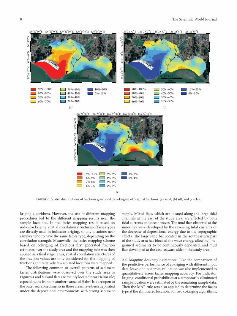
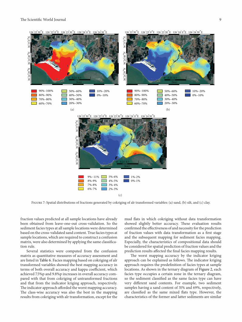