
Research Article An Effective Measured Data Preprocessing ...
16
Research Article An Effective Measured Data Preprocessing Method in Electrical Impedance Tomography Chenglong Yu, Shihong Yue, Jianpei Wang, and Huaxiang Wang School of Electrical Engineering and Automation, Tianjin University, Tianjin 300072, China Correspondence should be addressed to Shihong Yue; [email protected] Received 13 March 2014; Revised 11 May 2014; Accepted 26 May 2014; Published 22 July 2014 Academic Editor: Hak-Keung Lam Copyright © 2014 Chenglong Yu et al. is is an open access article distributed under the Creative Commons Attribution License, which permits unrestricted use, distribution, and reproduction in any medium, provided the original work is properly cited. As an advanced process detection technology, electrical impedance tomography (EIT) has widely been paid attention to and studied in the industrial fields. But the EIT techniques are greatly limited to the low spatial resolutions. is problem may result from the incorrect preprocessing of measuring data and lack of general criterion to evaluate different preprocessing processes. In this paper, an EIT data preprocessing method is proposed by all rooting measured data and evaluated by two constructed indexes based on all rooted EIT measured data. By finding the optimums of the two indexes, the proposed method can be applied to improve the EIT imaging spatial resolutions. In terms of a theoretical model, the optimal rooting times of the two indexes range in [0.23, 0.33] and in [0.22, 0.35], respectively. Moreover, these factors that affect the correctness of the proposed method are generally analyzed. e measuring data preprocessing is necessary and helpful for any imaging process. us, the proposed method can be generally and widely used in any imaging process. Experimental results validate the two proposed indexes. 1. Introduction Electrical impedance tomography (EIT) technique [1] is one nondestructive visualization measurement technology. Due to fast-response, noninvasive, low cost in obtaining 2D/3D distribution parameter information, EIT has been widely used in several principal areas such as medical imaging, industrial process imaging, and geophysical surveying [2]. But the EIT techniques are greatly limited to the low spatial resolutions [3–5] that greatly result from the following three problems. (1) Low Relative Resolution of Measurable Data. When these measuring data are of low relative resolution, that is, too small size difference of measuring data compared with their own sizes, the reconstructed EIT image is of low spatial resolution. In fact, most of the existing EIT imaging methods depend on an optimization process associated with a good relative solution of measurable data, while this process is an ill-conditioned, highly nonlinear, and uncertain problem [6]. If there are not good relative solutions of measurable data, the reconstructed images are of low resolution. us, an optimal measuring data preprocessing is necessary since the ill-conditioned equation is tightly associated with the meas- uring data. (2) Low Signal-to-Noise Ratio. e EIT measuring data are of low signal-to-noise ratio (SNR). Besides machine noise, owing to the use of weak current excitation, the measuring data in EIT must be a weak signal, and any small measuring errors or noise may lead to large spatial resolution of the investigated objects in an EIT image, or roughly speaking, any change of any objects in the investigated field could affect all measured data of all other objects in the investigated field. is is called “soſt-field” effect which is a much undesired case in practice [7, 8]. us, “soſt-field” effect is mainly responsible for the low SNR in the EIT imaging process [9, 10]. e existing ET imaging processes are unstable and oſten unacceptable in most noisy conditions [11, 12]. (3) Imaging Algorithm. A challenging problem in the EIT imaging process is how to quantitatively choose the proper algorithm to obtain the highest spatial resolution of EIT images. As a result, these reconstructed images usually do not have interpretability or understandability [13]. Some researchers attempt to solve this problem using simulation, Hindawi Publishing Corporation e Scientific World Journal Volume 2014, Article ID 208765, 15 pages http://dx.doi.org/10.1155/2014/208765
Transcript of Research Article An Effective Measured Data Preprocessing ...

Research ArticleAn Effective Measured Data Preprocessing Method in ElectricalImpedance Tomography
Chenglong Yu Shihong Yue Jianpei Wang and Huaxiang Wang
School of Electrical Engineering and Automation Tianjin University Tianjin 300072 China
Correspondence should be addressed to Shihong Yue shyue1999tjueducn
Received 13 March 2014 Revised 11 May 2014 Accepted 26 May 2014 Published 22 July 2014
Academic Editor Hak-Keung Lam
Copyright copy 2014 Chenglong Yu et al This is an open access article distributed under the Creative Commons Attribution Licensewhich permits unrestricted use distribution and reproduction in any medium provided the original work is properly cited
As an advanced process detection technology electrical impedance tomography (EIT) has widely been paid attention to and studiedin the industrial fields But the EIT techniques are greatly limited to the low spatial resolutions This problem may result from theincorrect preprocessing of measuring data and lack of general criterion to evaluate different preprocessing processes In this paperan EIT data preprocessing method is proposed by all rooting measured data and evaluated by two constructed indexes based on allrooted EIT measured data By finding the optimums of the two indexes the proposed method can be applied to improve the EITimaging spatial resolutions In terms of a theoretical model the optimal rooting times of the two indexes range in [023 033] andin [022 035] respectively Moreover these factors that affect the correctness of the proposed method are generally analyzed Themeasuring data preprocessing is necessary and helpful for any imaging process Thus the proposed method can be generally andwidely used in any imaging process Experimental results validate the two proposed indexes
1 Introduction
Electrical impedance tomography (EIT) technique [1] is onenondestructive visualization measurement technology Dueto fast-response noninvasive low cost in obtaining 2D3Ddistribution parameter information EIT has been widelyused in several principal areas such as medical imagingindustrial process imaging and geophysical surveying [2]But the EIT techniques are greatly limited to the low spatialresolutions [3ndash5] that greatly result from the following threeproblems
(1) Low Relative Resolution of Measurable Data When thesemeasuring data are of low relative resolution that is toosmall size difference of measuring data compared with theirown sizes the reconstructed EIT image is of low spatialresolution In fact most of the existing EIT imaging methodsdepend on an optimization process associated with a goodrelative solution of measurable data while this process isan ill-conditioned highly nonlinear and uncertain problem[6] If there are not good relative solutions of measurabledata the reconstructed images are of low resolutionThus anoptimal measuring data preprocessing is necessary since the
ill-conditioned equation is tightly associated with the meas-uring data
(2) Low Signal-to-Noise Ratio The EIT measuring data areof low signal-to-noise ratio (SNR) Besides machine noiseowing to the use of weak current excitation the measuringdata in EIT must be a weak signal and any small measuringerrors or noise may lead to large spatial resolution of theinvestigated objects in anEIT image or roughly speaking anychange of any objects in the investigated field could affect allmeasured data of all other objects in the investigated fieldThis is called ldquosoft-fieldrdquo effect which is a much undesiredcase in practice [7 8] Thus ldquosoft-fieldrdquo effect is mainlyresponsible for the low SNR in the EIT imaging process[9 10] The existing ET imaging processes are unstable andoften unacceptable in most noisy conditions [11 12]
(3) Imaging Algorithm A challenging problem in the EITimaging process is how to quantitatively choose the properalgorithm to obtain the highest spatial resolution of EITimages As a result these reconstructed images usually donot have interpretability or understandability [13] Someresearchers attempt to solve this problem using simulation
Hindawi Publishing Corporatione Scientific World JournalVolume 2014 Article ID 208765 15 pageshttpdxdoiorg1011552014208765
2 The Scientific World Journal
(a)
E1 E2E3
E4
E5
E6
E7
E8E9E10
E11
E12
E13
E14
E15
E16
(b) (c)
Figure 1 EIT imaging process (a) Original investigated objects of three blocks of watered agars (b) Each pixel is covered by 16 projectionfields (in grey) from 16 excitations (c) Reconstructed EIT image by the LBP algorithm based on measuring data
visualization and new hardware system for gaining com-parable statistics [14 15] but these methods are of littleapplicability in practice
The importance of the preprocessing processes of mea-suring data has been realized In order to obtain the EITimage of high resolution some researches attempt to adjustthe size of original measuring data based on the hardwaresystem For example the measuring data are amplified bya special integrated circuit However these methods con-centrate on asome linear transformations to all data whilea linear transformation cannot change the relative size ofthese measuring data When there are noisy data a lineartransformationwill simultaneously amplify signal and noisesIn this paper we present a nonlinear transformation to allmeasuring data In terms of rooting all measured data anEIT data preprocessing method is proposed and evaluated bytwo constructed indexes based on all rooted EIT measureddata One index aims to maximize the relative size amongmeasurable data and the other one aims to maximize SNRof the measuring data Dependent on their optimums of thetwo indexes the optimal root of the measuring data canbe obtained One purpose of rooting all data is to find theoptimal relative size of measurable data such that the EITspatial resolution of the EIT imaging can be improved greatlyAnother purpose of rooting the measuring data is to attain ashigh SNR as possible The research in this paper shows thatthe two proposed indexes have nearly the same optimumsbut different motivations The analytic optimal solutions ofthe two proposed indexes are obtained by a mathematicalanalysis The analysis of the two indexes involves the existingstudy [16] Recently the natural clustering structures hiddenin the EIT measuring data have been recovered and the fuzzyclustering algorithm termed as FC-EIT is proposed for EITimaging process The reconstructed images by the FC-EITalgorithm can obtainmuch higher spatial resolution in awiderange of parameter settings Particularly some experimentalresults from the FC-EIT algorithmare unable to be completedby other existing EIT algorithms at all In this research FC-EIT and other three existing EIT imaging algorithms areapplied to test the correctness of the two proposed indexes
The rest of this paper is organized as follows Section 2introduces the EIT imaging principle In Section 3 the
two indexes for measuring data preprocessing are pro-posed and analyzed in different conditions Experimentaltests and results of the two indexes are interpreted inSection 4 Section 5 is the conclusion
2 EIT Imaging Principle
As an example an ERT system of a total of 16 electrodesevenly distributed around a 16-centimeter radius pipe isapplied to illustrate the EIT imaging structure and processOriginal investigated objects are three blocks of watered agarsthat are put in salt water as shown in Figure 1
Figure 1(a) shows the investigated objects and the dis-tribution of 16 electrodes in an ERT system The adjacentexciting strategy is used for data collection that is amonga total of 16 pairs of electrodes when the exciting currentis added to one electrode pair (119894 119894 + 1) 15 voltage valuesof other electrodes are measured 119894 = 1 2 16 Afterexcitation electrode pair is switched 16 times 16 groups ofmeasurements are obtained amongwhich twomeasurementsincluding excitation electrode pairs need to be discarded dueto the large errors Consequently 13 groups of measurementsin each excitation are used for a frame of EIT imagereconstruction To reconstruct a frame of ERT image thecross-section is discretized by rectangular or triangular unitsrelated to pixels in the ERT image (see Figure 1(b)) Thecross-section boundary and any pair of equipotential linesconnected to two adjacent electrodes construct a projectionfield Each extraction electrode corresponds to 16 projectionfields (in grey) over the entire cross-section and thus anypixel in the cross-section must be covered by 16 projectionfields respectively from 16 different extraction electrodes Interms of these measuring data the investigated objects arevisually reconstructed (see Figure 1(c))
The EIT imaging process obeys the general Maxwellequation [5] whose simplified physical model for EIT can bewritten as
119880 = 119891 (120590 119868) = 119877 (120590) 119868 (1)
where119880 is the measured voltage vector on the electrodes sur-rounding the periphery of a subject 119868 is the injected current
The Scientific World Journal 3
vector 120590 is the conductivity distribution in a cross-sectionof the subject 119891(120590 119868) is the nonlinear model mapping 120590
and 119868 to 119880 and 119877(120590) is the model mapping 120590 to resistanceThis model depends nonlinearly on the conductivity 120590 andlinearly on the current 119868 The aim of image reconstructionfor EIT is to obtain the conductivity distribution 120590 using theboundary voltage vector 119880 and the injected current vector 119868The mathematical expression of the tomographic problem isgiven by the following equations
[Δ119880]119870times1 = [119880]119870times119873 sdot [Δ119866]119873times1 or 119880 = 119878119866 (2)
where 119878 is a Jacobian matrix that is the sensitivity distribu-tion and 119870 and 119873 are the numbers of total measurementsand pixels respectivelyThe goal is to determine the unknownimage 119883 when the experimental projections 119880 are availableIn the discrete form the aim of image reconstruction for theEIT field is to find the unknown pixel vector from the known119880 by using (2) that is
119866 = 119878minus1119880 (3)
However the direct analytical solution for (3) does notexist since the inverse problem is both nonlinear and ill-posed and little noise in the measured data could cause largeerrors in the estimated conductivity Many algorithms havebeen proposed to indirectly solve the above ill-posed problemas explained below
(1) LBP AlgorithmThe most used EIT image reconstructionalgorithm is the linear back projection (LBP) [6] In theLBP algorithm the conductivity distributions are assumed tocomprise a number of discrete regions within the measure-ment space such that the conductivity within each region isconstant According to (3) 119860minus1119861 is approximated as
119866 =119878119879119880
119878119879119880120582
st 119880120582= [1 1 1] (4)
Equation (4) shows that the grey value of any pixel is calcu-lated by using a weighted form in the LBP algorithm
(2) Landweber Algorithm The Landweber algorithm (LW)[14] was originally designed for solving the classical ill-posed problem using the strategy similar to the gradientdescending algorithm in the optimization process by thefollowing equation
119866119905+1
= 119866119905minus 120572119878119879(119878119866119905minus 120582) (5)
where the constant 120572 is known as the gain factor and isused to control the convergence rate As the iterative processdescribed by (5) proceeds the norm of the capacitanceresidual will be minimized Since the norm may tend to bea certain value larger than zero the original algorithm oftenis modified as
119866119905+1
= 119875 [119866119905minus 120572119878119879(119878119866119905minus 120582)] (6)
The value of 119875 has been adopted by inclusion of a nonlinearfunction to constrain the estimated image so that 119866
119905+1isin
[0 1] that is when a normalized gray level is less than zeroit is constrained to be zero and when it is larger than ldquo1rdquo it isconstrained to be ldquo1rdquo
(3) Tikhonov Regularization The Tikhonov regularization(TR) [15] is one efficient method and is presented as a mini-mization function shown as follows
119869 (119892) =1
2119880 minus 119878120590
2+ 120583119877 (120590) (7)
where119877(119892) is the regularization function and 120583 is the regular-ization parameter The function is often expressed in 119871
2 formas
119877 (119892) = 119871 (120590 minus 120590)2 (8)
where 119871 is an appropriate regularization matrix and 120590 is aprior estimate of the permittivity or the conductivity distri-bution
(4) FC-EIT Algorithm Recently one efficient and originalEIT imaging algorithm [16] termed as FC-EIT has beenproposed FC-EIT firstmaps119870measuring data of pixel 119895 after119870 excitations into a 119870-dimensional vector as
(V1198951V1198952 V
119895119870)119879
forall119895 = 1 2 119899 (9)
All vectors associated with all pixels consist of a set 119883 andthen all vectors in119883 are partitioned into 119888 clusters by the fuzzy119888-means (FCM) algorithm [17] Let 119906
119894119895be the membership
degree of 119895th vector (pixel) to 119894th cluster let V119894be the cluster
prototype of 119894th cluster and let 119866(V119894) be the gray value of 119894th
cluster prototype 119894 = 1 2 119888 119895 = 1 2 119899 So the grayvalue of 119895th pixel 119892(119895) is determined by the weighted averageform
119892 (119895) =
119888
sum
119894=1
119906119894119895119866 (V119894) 119895 = 1 2 119899 (10)
All pixels are endowed with different gray values based on(10) These determined gray values thus can reconstruct aframe of EIT image to show various conductivities and torecover the distributions of investigated objects in the cross-section
LBP is a typical noniterative algorithm and has the leastexcusive time and the others are iterative algorithms andneed more runtime These EIT imaging algorithms are themost used ones in practice In this paper the above algo-rithms are applied for EIT imaging reconstruction to examinethe spatial resolutions before and after performingmeasuringdata preprocessing
3 Optimal Data Preprocessing Method
In this section we define a relative size (RS) index and asignal-to-noise ratio (SNR) index of the measureable datarespectively The optimums of the two indexes are appliedto realize the optimal measuring data preprocessing andimprove the EIT spatial resolution The characteristics of thetwo indexes are illustrated below
4 The Scientific World Journal
(a) Original model of 2 cycles
Original dataSquare rootFifth root
0 50 100 150 200 2500
005
035
01
015
02
025
03
(b) Original and rooted measuring data
Figure 2 Extraction of roots for the measured data
31 Two Quantitative Indexes for Evaluating Data Preprocess-ing Process The relative sizes of 119870 measuring data of anypixel after 119870 excitations can lead to great differences for theEIT spatial resolution Due to the weak current excitation inEIT most of the measuring data have very small size Thusamplifying the original data to a proper size is a necessary stepfor the EIT imaging process [2 12] The larger measureabledata relative size the higher EIT images spatial resolution [1216] The first proposed index aims to maximize the relativesize by using a nonlinear transformation of all measuringdata because a linear amplification must keep the relativesizes being a constant Assuming that an investigated fieldis partitioned into 119899 pixels a nonlinear transformation isperformed by finding 119911 root to all measuring data as in thefollowing form
119910119896119895
= 119911radicV119896119895 119896 = 1 119870 119895 = 1 2 119899 (11)
where V119896119895
is the measured data of the 119895th pixel in the 119896thexcitation 119896 = 1 2 119870The proposed index termed as therelative size (RS) index is defined as
120585 =
119899
sum
119895=1
119870
sum
119904119905=1
(max 119910119895119904 119910119895119905 minusmin 119910
119895119904 119910119895119905)
119899 (119870 minus 1) (12)
where 119904 and 119905 are two consecutive integers and V119895119904
and V119895119905
are two successive measuring data from the two successiveexcitations The value of 120585 totally reflects the relative size ofmeasuring data of all pixels Tomaximize the relative size theoptimum of (12) is solved as
119911lowast= arg max
119911120585 (13)
Independent of any measuring data and any EIT imagingalgorithms (13) must have a maximum at least for any setof pixels associated with these investigated objects due to thefollowing three reasons
(A) For 120585 ≧ 0 the inequality holds from (12)(B) For 120585 = 0when 119911 rarr infin119910
119894119895rarr 1 the equation holds
since zero exponents of any number are 1 and thus areequivalent to each other
(C) For 120585 asymp 0when 119911 rarr 1 all measuring data keep theiroriginal values and the mutual differences of thesedata are very small
Equation (13) shows that the optimal measuring data can besolved by the optimum of the RS index of (13) Thus theoptimal determination of the rooting times of the measuringdata can enhance their relative sizes
Figure 2(a) shows an original image that is simulatedin Comsol simulation environment [18] The reconstructedobjects are two circles with conductivity 200 and the cor-responding background with conductivity 100 Figure 2(b)shows the simulated measurable data associated with theoriginal image It is difficult to identify these measuringdata in terms of their original relative sizes As comparedthe second and the fifth roots of these measurable data areshown in the same coordinate Compared with the originalmeasuring data their relative sizes become larger In facttheir values of 120585 are 1212 and 1930 respectively whilethe value of 120585 of the original measuring data is 273 Thisdemonstrates that extracting the root of measurable data canincrease their relative sizes
On the other hand for 119870 measuring data of any pixelthere are seriously noisy data and ldquosoft-fieldrdquo effects Usuallythe two measuring data that are closest and farthest to a pairof exciting electrodes are of low SNRThe closest one is due tothe strong proximity effect between exciting and measuringelectrodes and the farthest one is prone to be affected bythese polarization effects and ldquosoft-fieldrdquo effects in the fieldConsequently these measuring data that are nearly located inthemiddle between the closest and farthest electrodes are the
The Scientific World Journal 5
(a) Original image
035
0 50 100 150 200 2500
005
01
015
02
025
03
Original dataSquare rootFifth root
(b) Original and preprocessing data
Figure 3 Original image and effects of rooting measuring data
most effective among 119870 measuring data The second indexaims to minimize the effect of the two measuring data byfinding their optimal root by (11) So the second index termedas the SNR index is defined as
120578 =2
119899119870
times
119899
sum
119895=1
sum119870
119896=1V119895119896
maxV1198951 V1198952 V
119895119896+minV
1198951 V1198952 V
119895119896
(14)
where maxV1198951 V1198952 V
119895119896 and minV
1198951 V1198952 V
119895119896 are
the farthest and closest measuring data in119870measuring datarespectively The coefficients of 2119899119870 make the values of 120578equal to 1 when all values of V
119895119896are equivalent to each other
It is clear that the larger the values of 120578 are the higher the SNRisThus values of 120578 can show the SNR level of thesemeasuringdata To obtain the highest SNR (14) is solved by
119911lowast= arg max
119911120578 (15)
The optimum of (15) shows the SNR level of the measuringdata after finding the optimal root Equation (15) must havea maximum at least for any set of pixels associated with theseinvestigated objects due to the following three reasons
(A) For 120578 ≧ 1 the inequality holds from (14)(B) For 120578 asymp 1when 119911 rarr 1 all measuring data keep their
original values and the mutual differences of thesedata are very small
(C ) For 119899 = 1 when 119911 rarr infin 119910119894119895
rarr 0 the equationholds since the infinite roots of any numbers are 1 andthus are equivalent to each other
Figure 3 shows a simulation in Comsol simulation envi-ronment [18] the original image consists of three circles withthe same conductivity as well as background The simulatedmeasuring data shown in their optimal 3rd root Compared
with the original measuring data the data after finding theirroots havemuch larger values of 120578This demonstrates that therooting operation is helpful in improving the SNR level
32 Optimal Solution of the Two Proposed Indexes The cross-section in an EIT system is called a full field when theinvestigated objects are contained and otherwise is called anempty fieldThe optimums of (13) and (15) are solved in a fullfield However it is impossible to obtain an analytic optimumfor an arbitrary full field owing to extremely complex distri-butions of investigated objects Notice that the relative sizesof measuring data in a full field are nearly proportional tothose in the empty field [12 13] Consequently the optimumsof (13) and (15) are solved in an empty field Without lossof generalization a system of 16 electrodes is taken in acircular investigated field as an example For each excitation13 measuring data consist of a U-shaped curve and allmeasuring data from 16 excitations are summed up to 208for the same pixel as shown in Figure 4(a) Assume that1198791 1198792 1198793 1198794 1198795 1198796 and 119879
7are 7 electrodes on a circular
empty field as shown in Figure 4(b)The circle equation with radius 119877 in a polar coordinate
system can be formulated as
120588 = 2119877 sin 120579 (16)
where 120588 is polar radius and 120579 is polar angle Each pair ofexciting electrodes 119860 and 119861 is regarded as an electric dipolesince they have enough small distance compared with theradius of the circled field The polar coordinate equation onthe equipotential line in arbitrary 119875 point in the investigatedfield is shown as
120588 = 119862radiccos 120579 (17)
where 119862 is the potential value of the equipotential line thatgoes through 119875 point According to the basic mathematical
6 The Scientific World Journal
0 50 100 150 200 2503000
4000
5000
6000
7000
8000
9000
(a) 16 U-shaped curves
120588 =
T7(1205887 1205797)
T6(1205886 1205796)
T5(1205885 1205795)
T4(1205884 1205794)
T3(1205883 1205793)
T2(1205882 1205792)
T1(1205881 1205791)
0A B
120588 = Cradiccos 120579
P(120588 120579)
x
2R sin120579
(b) Polar coordinate system
Figure 4 Measuring data with U-shaped curve and polar coordinate system
theorem [19] the same arc has equivalent angle in a circularsegment drawing out the following relation
ang11987911198741198792= ang11987921198741198793= sdot sdot sdot = ang119879
61198741198797 (18)
Let the polar coordinates 1198791 1198792 119879
7be (1205881 1205791) (1205882 1205792)
(1205887 1205797) after the polar point is taken as the center of the
exciting electrodes 119860 and 119861 respectively To begin with 119909-axis at the 119896th excitation these polar angles 119879
1 1198792 119879
7are
represented as
120579119894= (
2120587
15119894)
0
asymp (24119894)0 119894 = 1 2 7 (19)
After combining (16) and (17) the potential values of 1198791sim 1198797
are solved as
119862 =2119877 sin 120579
radiccos 120579997904rArr 119862
119894=
2119877 sin 120579119894
radiccos 120579119894
= 119876119894119877 119894 = 1 2 7
(20)
where 119876119894= 2 sin 120579
119894radiccos 120579
119894 119894 = 1 2 7 are 7 invariant
constants when the number of electrodes 119870 is fixed Thepotential relative sizes of these measuring data among theseven electrodes 119879
1 119879
7are
V119895119896
= 119906119895119896+1
minus 119906119895119896
= (119876119895119894+1
minus 119876119895119894) 119877
119895 = 1 2 119899 119896 = 1 2 7
(21)
Generally owing to V1198951
gt V1198952
gt sdot sdot sdot gt V1198957
and 119911radic1198701198952
minus 1198701198951
gt
119911radic1198701198953
minus 1198701198952
gt sdot sdot sdot gt 119911radic119870119895119870+1
minus 119870119895119870
therefore (13) and (15)can be rewritten as
120585 =
119899
sum
119895=1
119896
sum
119904119905=1
( 119911radic119876119895119904+1
minus 119876119895119904
minus 119911radic119876119895119905+1
minus 119876119895119905)119911
radic119877
119899 (119870 minus 1)
120578 =2
119899119870
119899
sum
119895=1
sum119870
119896=1119911radic119876119895119896+1
minus 119876119895119896
119911radic1198701198953
minus 1198701198952
+ 119911radic119870119895119870+1
minus 119870119895119870
(22)
2 4 6 8 10 12 14minus001
001
002
003
004
005
006
007
008
009
0
0
Original dataSquare rootFifth rootTenth root
Twentieth rootThirtieth rootFortieth root
Figure 5 Variance of U-shaped curves after rooting the measuringdata
When the number of electrodes is fixed the optimums of (13)and (15) are two constants and can be solved easily Accordingto the finite element method [20] when 119870 = 16 for ERT and119870 = 12 for ECT the optimums of (1119911) in (13) are 026 and034 and the optimums in (15) are 023 and 033 respectively
According to the two original images in Figures 2 and3 Figure 5 shows the optimal solutions of (13) and (15)Figure 5 shows that the relative sizes of the measuring datagradually increase from 01 to 026 and decrease from 026 to01 where all origins of U-shaped curves after rooting thesemeasuring data are located in the same point
Both (13) and (15) can provide the optimalmeasuring datapreprocessing according to the same rooting operation in (11)
The Scientific World Journal 7
but are based on different motivations In the experimentalpart in this paper our research shows their interrelations
33 The Correctness of the Two Proposed Indexes The opti-mums of the two proposed indexes are solved under thisassumption that variances of the measuring data are nearlydirectly proportional to each other in the empty and fullfields However a real investigated field can be affected byvarious and complex applicable conditions and thus it isnecessary to consider the correctness of the two indexesin these conditions Generally the investigated objects in afield consist of materials with different attributes such asconductivity permittivity and permeability The materials ofthe same attribute must have the similar distribution of themeasuring data while the ones of different attributes have dif-ferent distributionsThe same distributions of measured datacorrespond to the same cluster while different distributionscorrespond to different clusters Consequently the task of ETimaging aims to find all clusters of measuring data [12 16]Most of the actual investigated objects consist of clusters withvarious characteristics such as sizes densities and positionsSo in this paper the three characteristics are generally definedto evaluate the effect of the two proposed indexes as follows
The quantity to show position characteristic is computedas
position (119888) =
119888minus1
sum
119894=1
119888
sum
119895=119894+1
max (119875119894 119875119895) min (119875
119894 119875119895)
1198622119888
(23)
where 119875119896represents the minimal distance to the 119896th clus-
ter from other clusters and is computed by all pairwisedistances from the 119896th cluster to the closest cluster for119896 = 1 2 119888 Clearly position(119888) gt 1 since the valueof max(119875
119894 119875119895)min(119875
119894 119875119895) must be larger than 1 Values of
position(119888) are smaller and distributions among clusters aremore consistent and symmetric Thus values of position(119888)can efficiently show the characteristics of relative positionamong all clusters
The quantity to represent size characteristic is computedas
size (119888) =119888minus1
sum
119894=1
119888
sum
119895=119894+1
max (119878119894 119878119895) min (119878
119894 119878119895)
1198622119888
(24)
where 119878119896refers to the size of 119896th cluster and is computed by
the average of all pairwise distances between the two datavectors in 119896th cluster for 119896 = 1 2 119888 Clearly size(119888) gt
1 since the value of max(119878119894 119878119895)min(119878
119894 119878119895) is larger than 1
Values of size(119888) are smaller and sizes among clusters aremore consistent Thus values of size(119888) can efficiently showthe characteristics of relative size among all clusters
The quantity to show density characteristic is computedas
density (119888) =119888minus1
sum
119894=1
119888
sum
119895=119894+1
max (119863119894 119863119895) min (119863
119894 119863119895)
1198622119888
(25)
where 119863119896represents the density of 119896th cluster and is com-
puted by a division between the number of data vectors and
119863119896in the 119896th cluster Clearly density(119888) gt 1 for the value of
max(119863119894 119863119895)min(119863
119894 119863119895) is larger than 1 Smaller values of
density(119888) show that all clusters have nearly the same numberof data vectorsThus values of density(119888) can efficiently showthe characteristics of relative density among all clusters
To begin with a dataset of three clusters we reconstruct220 three cluster-contained datasets of different characteris-tics by changing one quantity and changing a pair of quan-tities related to the above three characteristics respectivelyFigures 6(a) 6(c) and 6(e) show three representative datasetswhen changing one of the three quantities respectively Asthese quantities are changed their determined optimumsof the RS index are shown in Figures 6(b) 6(d) and 6(f)Figure 6 shows that in a wide sampling range position(119888) isin
[1 3] size(119888) isin [1 4] and density(119888) isin [1 4] each quantityin itself has little effect on the determined optimum of theproposed index
Figures 7(a)ndash7(c) show the effect of three pairs of com-bined quantities for the optimums of the RS index Whenposition(119888) gt 31 and size(119888) gt 28 the optimum of the RSindex is 024 when size(119888) gt 36 and density(119888) gt 38 the oneis 026 and for position(119888) isin [1 3] and size(119888) isin [1 4] the oneis around 03 When the above three pairs of combinationstake the other values the determined number of all clustersis 5 Thus the combined quantities of position(119888) and size(119888)play a major role in the optimum of the RS index size(119888)and density(119888) play a second important role and position(119888)and density(119888) have no apparent effect on the final optimumsPlease note that position(119888) isin [1 3] size(119888) isin [1 4] anddensity(119888) isin [1 4] are very general conditions and areencountered in most real applications
In sum the RS index has the following key characteristicsThe optimum of the RS index can keep unchangeable in awide range of various characteristics and thus is robust tosatisfy the general needs in practice If the number of excitingelectrodes is fixed this optimum is a constant The optimumof the RS index assures the effectiveness and generalizationof the EIT imaging process The SNR index behaves as theRS index but they have different motivations and applicableranges The experimental part in this paper will present theirrelative sizes and interrelations
4 Experiments
Two groups of experiments are applied to validate the twoproposed indexes in Comsol simulation and real test respec-tively The spatial resolution of EIT sensitive field is definedas the total relative error of all pixels in the reconstructed EITimage and formulated as
120585 = (1
119870)
119870
sum
119895=1
(119892119895minus 119892lowast
119895)
119892lowast
119895
(26)
where 119892119895is the reference gray value of the 119895th pixel and is
known as a prior or real measuring data 119892lowast119895is the gray value
8 The Scientific World Journal
(a) Original model
008012
01602
0 5 15 25 3510 20 30 40
150
250200
350300
400450
200
250
300
350
400
450
Times of rootR
r
(b) Effect of cluster size
(c) Original model
045055 05 040607 065075
051015
2025
30
100150200250300350
Distance to center
Times of root
160140
180
220
320300280260240
200
r
(d) Effect of cluster distributions
100 200
10
(e) Original model
481216200 5 10 15 20 25 30
200250300350400450500550
Conductivity
r
250
500
450
400
350
300
Times of root
(f) Effect of conductivity magnitude
Figure 6 Effect of various characteristics on the optimum of the RS index (a) (c) and (e) are six original images and (b) (d) and (f) arethe curves of the optimums by the index
of the 119895th pixel after an EIT image 119895 = 1 2 119870 and 120585 isthe average of the total error of all the119870 pixels
The four algorithms LBP TR LW and FC-EIT areapplied to the EIT imaging process to test the correctness ofthe two proposed indexes
41 Simulation in Comsol Environment The group of exper-iments is implemented in Comsol simulation environment[18] An EIT system of 16 electrodes is set up The originalimages consist of two three four and five circles with contin-uously distributedmaterials respectively as shown in the first
The Scientific World Journal 9
(a) Curve 1
R
6789
1110
12
04045
05055
06065
07 02018
016014
012Distance to center
01
11
108
106
104
102
10
98
96
94
92
9
Nth
root
(b) Effect of cluster size and distributions
(c) Curve 3
6
26
10
ConductivityDistance to center
1418
1098
9496
92988
8486
828
04 045 05 055 06 065 07
8
109
7
1211
Nth
root
(d) Effect of cluster size and position
10
100 200
(e) Curve 5
00801 012
014 016018
02
4 2
8 6
16 14 1210
2018
61012
8
Size
Conductivity88284868899294969810
Nth
root
(f) Effect of cluster conductivity and position
Figure 7 Effect of various three pairs of characteristics on the optimum of the RS index (a) (c) and (e) are six original images and (b) (d)and (f) are the curves of the optimums by the RS index
row in Figure 14 These circles have the same conductivityand thus should be shown as the same gray degree in anyEIT image while the background has another gray valueThe ratio of conductivity between the circles and background
is set to 4 1 By the adjacent excitation way the measuringdata are produced According to (12) and (15) we take theoptimal values of theRS index and the SNR index individuallyas 119911 = 35 and 119911 = 39 In terms of these roots to all
10 The Scientific World Journal
minus08
minus05minus1minus1
minus06
minus04
minus02
08
05035
0503
05025
0502
05015
0501
05005
05
04995
0499
06
04
02
05
1
1
0
0
(a) Image before adding noisy data
minus08
minus05minus1minus1
minus06
minus04
minus02
08
066
064
062
06
058
056
054
052
05
048
06
04
02
05
1
1
0
0046
(b) Image after adding noisy data
Figure 8 Contrast of the reconstructed images after and before adding the optimal root
measuring data these circles in these original images arereconstructed Figure 14 shows these circles before and afterfinding the optimal root to all measuring data Comparedwith the original images the reconstructed circles based onthe RS index are clear and nearly consistent after rootingall measuring data Additionally the trail traces in an EITimage can visually evaluate the spatial resolution of the imageIt can be observed that the trail traces in these EIT imagesare widely distributed without data preprocessing and evensome circles are incorrectly connected to the same areaParticularly Figure 14 shows that the Landweber algorithmcan distinguish these circles better than the other threealgorithms and reconstructed images have much smallertrail traces under a wide range of parameter settings Theseresults further demonstrate that the Landweber algorithmoutperforms the other three algorithms in the four groupsof datasets and has much smaller trail traces In fact theaverage spatial resolution of these images can be raised by175 by finding the optimal root of measuring data Ascompared when 119911 = 39 the SNR index can improvespatial resolution about 127 according to (26) Notice thatthe Comsol simulation is set without noisy data and thusthe RS index may give higher improvement than the SNRindex On the other hand the highest resolutions of the fourmodels are 34 38 45 and 27 respectively The error of theoptimum is assured by the assumption that the actual datais directly proportional to the real increment of measuringdata But it should be noted that the two proposed indexeshave no mathematical basis at present and this can be furtherimproved
When the noisy data are added into the measured datathe spatial resolution of the reconstructed EIT must reduceBut the proposed method of rooting operation can slightlybe affected and is far away from the optimums about 10Figure 8 shows two reconstructed EIT images before andafter 15 noisy data where the optimal rooting values are
038 and 034 for RS and SNR respectively while theirtheoretical optimal solutions of (13) and (15) are 036 and 035respectively
42 Test on an ECT Field In the experiment two movableglass rods are inserted into a measuring pipe and the back-ground material is air as shown in Figure 9 A 16-electrodeECT sensor is equipped on a cross-section of the pipe toexcite and obtain the measuring dataThemeasuring processis repeated 20 times for different positions of the two rodsto form data sequence sampling There are noisy signals inthis sampling process Thus the SNR index is applied tomeasuring data preprocessing to decrease the effect of thenoisy signal as much as possible
Figure 10 shows the measuring data distribution beforeand after finding their optimal roots According to the opti-mum of the SNR index the measuring data before findingthe optimal root are irregular and some of them deviatefrom the traces of U-shaped curve Particularly some meas-uring data are mixed with each other due to quite smallrelative size Thus these data may produce trail traces in thereconstructed EIT images and inevitably decrease the spatialresolution Such partial data are caused by the machine noisein the sampling process besides the ldquosoft-fieldrdquo effect Insteadafter finding the optimal root these measuring data becomeregular Their relative sizes become larger than those beforefinding the optimal root
In terms of these measuring data before and after findingthe optimal root the LBP algorithm is applied to reconstructthe two rods as shown in Figure 11 The two reconstructedrods after finding the optimal root aremuch clearer and tidierthan before According to the values of (26) in 20 times ofexperiments the former averagely is 035 and the latter is 047Consequently the spatial resolutions of these EIT images are
The Scientific World Journal 11
(a) The measuring equipment (b) The cross-section of the measuring sensor
Figure 9 The measuring equipment and investigated objects
0 50 100 150 200 250
times10minus3
14
12
1
08
06
04
02
0
(a) Data before finding the optimal root
0 50 100 150 200 2500
0005
001
0015
002
0025
003
0035
004
(b) Data after finding the optimal root
Figure 10 Contrast of the measured data after and before finding the optimal root
minus08
minus1
minus06
minus04
minus02
08
06
04
02
1
0
minus05minus1 05 1
5
6
7
8
9
10
11
12
13
14
15
0
(a) Image before finding the optimal root
minus08
minus1
minus06
minus04
minus02
08
06
04
02
1
0
minus05minus1 05 1
15
14
13
12
11
10
9
8
7
6
5
0
(b) Image after finding the optimal root
Figure 11 Contrast of the EIT images after and before finding the optimal root
12 The Scientific World Journal
minus08
minus1
minus06
minus04
minus02
08
06
04
02
1
0
minus05minus1 05 10
minus1
1
2
3
4
5
6
0
times10minus4
(a) Image before finding the optimal root
minus08
minus05minus1
minus1
minus06
minus04
minus02
08
06
04
0
0
1
1
minus2
0
2
4
6
8
10
12
14
16
18
02
05
times10minus3
(b) Image after finding the optimal root
Figure 12 Contrast of the reconstructed images after and before finding the optimal root
minus08
minus1
minus06
minus04
minus02
08
06
04
02
1
0
minus05minus1 05 1
6
8
10
12
14
16
18
20
22
0
(a) The image before rooting all measuring data
minus08
minus1
minus06
minus04
minus02
08
06
04
02
1
0
minus05minus1 05 15
10
15
20
0
(b) Image after rooting all measuring data areas
Figure 13 Contrast of the reconstructed images after and before finding the optimal root
greatly improved based on the SNR index In addition theproposed data preprocessing process hardly needs to be at theexpense of extra runtime since the process to find the optimalroot needs much less runtime than the EIT imaging processitself
When the RS index is applied to data preprocessing andthe LBP algorithm is applied to reconstruct the two rods asshown in Figure 12 the increment of spatial resolution of theEIT image from the RS index is not as large as that from theSNR index In fact the values of (26) based on the RS indexare averagely 233 Thus the SNR index is more suitable forthe noisy condition while theRS index ismore accuratewhenmeasuring data conclude little noise or are simulated data
When the rooting times in the RS index are taken from 02 to08 the spatial resolutions of all reconstructed images can beimproved with different extents Thus the rooting operationis a very useful data preprocessing method for the originalmeasuring data
When the target objects are located in centric andboundary areas respectively the optimal rooting values haveapproximately the same results even though the spatial reso-lutions in the two areas are very different But the reformu-lations of the spatial resolution are very limited for the EITimages In the average meaning the spatial resolution in thecentric area reduces to 60 as much as that in the boundaryarea as shown in Figure 13
The Scientific World Journal 13
0
012013 013
01401501601701801902021
01301401501601701801902021
013012
01401501601701801902021
01401501601701801902
0051152253354455
00080010012001400160018002
12345
05115225335445
0
0
0
0
005
01
015
02
051152253354
012345
012345
05 5
10 10
15 15
2020
12345
05101520
0
5
10
15
012345678
012345678
012345
0051152253354
05101520
0
5
1015
20
Two circlesData set
Original model
Three circles Four circles Five circles
LBP
LW
TR
times10minus4
times10minus4
times10minus3
times10minus4
times10minus3times10minus3 times10minus3
times10minus4 times10minus4 times10minus4
times10minus3 times10minus3 times10minus3
times10minus4 times10minus4times10minus4
times10minus4 times10minus4
08060402
1
0minus02minus04minus06minus08minus1
08060402
1
0minus02minus04minus06minus08minus1
08060402
1
0minus02minus04minus06minus08minus1
08060402
1
0minus02minus04minus06minus08minus1
08060402
1
0minus02minus04minus06minus08minus1
08060402
1
0minus02minus04minus06minus08minus1
08060402
1
0minus02minus04minus06minus08minus1
08060402
1
0minus02minus04minus06minus08minus1
08060402
1
0minus02minus04minus06minus08minus1
08060402
1
0minus02minus04minus06minus08minus1
08060402
1
0minus02minus04minus06minus08minus1
08060402
1
0minus02minus04minus06minus08minus1
08060402
1
0minus02minus04minus06minus08minus1
08060402
1
0minus02minus04minus06minus08minus1
08060402
1
0minus02minus04minus06minus08minus1
08060402
1
0minus02minus04minus06minus08minus1
08060402
1
0minus02minus04minus06minus08minus1
08060402
1
0minus02minus04minus06minus08minus1
08060402
1
0minus02minus04minus06minus08minus1
08060402
1
0minus02minus04minus06minus08minus1
08060402
1
0minus02minus04minus06minus08minus1
08060402
1
0minus02minus04minus06minus08minus1
08060402
1
0minus02minus04minus06minus08minus1
08060402
1
0minus02minus04minus06minus08minus1
0 105minus05minus1
0 105minus05minus1
0 105minus05minus1
0 105minus05minus1 0 105minus05minus1 0 105minus05minus1 0 105minus05minus1
0 105minus05minus1 0 105minus05minus1 0 105minus05minus1
0 105minus05minus1 0 105minus05minus1 0 105minus05minus1
0 105minus05minus1 0 105minus05minus1 0 105minus05minus1
0 105minus05minus1 0 105minus05minus1 0 105minus05minus1 0 105minus05minus1
0 105minus05minus1 0 105minus05minus1 0 105minus05minus1 0 105minus05minus1
minus1 minus1
minus1minus2minus1
minus5 minus5 minus5
minus05 minus1minus05minus1
minus5
0510152025
minus5
LBP minus 1
LW minus 1
TR minus 1
Figure 14 Continued
14 The Scientific World Journal
16141210
864
161412108645
6789101112131415
56789101112131415
56 6
4 56789101112131415 16
14121086
78 8910 101112 121314 1415
FC-EIT
FC-EIT
08060402
1
0minus02minus04minus06minus08minus1
08060402
1
0minus02minus04minus06minus08minus1
08060402
1
0minus02minus04minus06minus08minus1
08060402
1
0minus02minus04minus06minus08minus1
08060402
1
0minus02minus04minus06minus08minus1
08060402
1
0minus02minus04minus06minus08minus1
08060402
1
0minus02minus04minus06minus08minus1
08060402
1
0minus02minus04minus06minus08minus1
0 105minus05minus1
0 105minus05minus1 0 105minus05minus1 0 105minus05minus1 0 105minus05minus1
0 105minus05minus1 0 105minus05minus1 0 105minus05minus1
Two circlesData set Three circles Four circles Five circles
Figure 14 Test on the effect of finding the optimal root of measuring data Note ldquo119909rdquo and ldquo119909 minus 1rdquo are the EIT images before and after rootingthe measuring data respectively
5 Conclusion
In this paper a nonlinear transformation method of opti-mally rooting all measuring data is proposed to improvethe EIT spatial resolution The optimal rooting times aredetermined by two constructed indexes for measuring datapreprocessing The rooting operation has the followingadvantages
(1) Easy OperationThe simple rooting operation of measur-ing data is very easy to be implemented in software and hard-ware systems Moreover various EIT techniques can followthe same way in practice
(2) Robustness The spatial resolution of EIT images can beimproved in a very wide range of the rooting values as wellas their optimums This characteristic is very suitable forengineering applications
(3) EffectivenessThe proposed method has been validated infour most used EIT imaging algorithms and can hold in mostEIT algorithms
(4) Different Effects The SNR index is more suitable undernoisy conditions while the RS index works better in simu-lated or hardly free-noisy conditions when applying an EITsystem Moreover to our knowledge so far there is no quan-tity to measure the characteristics of investigated objects invarious conditions so these three quantities proposed in thispaper are valuable for further setting a uniform criterion tocompare various imaging processes and different algorithms
There is a great room to improve the two proposedindexesWhile promising our immediate next studies will beas follows
(1) The use of the sensitive coefficients in the investi-gated field could generate vectors of more accuratecharacteristics to find more effective nonlinear toolinstead of the rooting operation The use of sensitive
coefficients can provide better spatial resolutionswhich has been demonstrated in the existing ETimage algorithms
(2) The second study will be concerned with determiningdifferent weighting values for different componentsof all vectors The existing study has shown that themeasured data in different electrode pairs containdifferent noise-signal ratios and thus have differenteffects on the final EIT imaging results Consequentlythe use of different weight values to present thesedifferent effects is preferable to enhance the imagingspatial resolutions
(3) The third study will be on the use of other nonlin-ear transformations to measurable data besides therooting operation Various nonlinear transformationtechniques have been developed for decades andvarious research ways and achievements are rich andefficient
Conflict of Interests
The authors declare that there is no conflict of interestsregarding the publication of this paper
Acknowledgments
Thiswork is supported by theNational Science Foundation ofChina (Grants nos 61174014 and 60772080) and the NationalScience Foundation of Tianjin (Grant no 08JCYBJC13800)
References
[1] Q Marashdeh L Fan B Du andWWarsito ldquoElectrical capac-itance tomographymdasha perspectiverdquo Industrial amp EngineeringChemistry Research vol 47 no 10 pp 3708ndash3719 2008
[2] B Du W Warsito and L Fan ldquoImaging the choking transitionin gas-solid risers using electrical capacitance tomographyrdquo
The Scientific World Journal 15
Industrial and Engineering Chemistry Research vol 45 no 15pp 5384ndash5395 2006
[3] W Yin andA J Peyton ldquoA planar EMT system for the detectionof faults on thinmetallic platesrdquoMeasurement Science and Tech-nology vol 17 no 8 article 011 pp 2130ndash2135 2006
[4] Z Cao HWang and L Xu ldquoElectrical impedance tomographywith an optimized calculable square sensorrdquo Review of ScientificInstruments vol 79 Article ID 103710 2008
[5] H William J Hayt and J Buck Engineering ElectromagneticMcGraw- Hill New York NY USA 7th edition 2006
[6] F Santosa and M Vogelius ldquoA backprojection algorithm forelectrical impedance imagingrdquo SIAM Journal on Applied Math-ematics vol 50 no 1 pp 216ndash243 1990
[7] M Cheney D Isaacson J Newell S Simske and J GobleldquoNOSER an algorithm for solving the inverse conductivityproblemrdquo International Journal of Imaging Systems and Technol-ogy vol 2 no 2 pp 66ndash75 1990
[8] S H Yue T Wu L J Cui and H X Wang ldquoClusteringmechanism for electric tomography imagingrdquo Science ChinaInformation Sciences vol 55 no 12 pp 2849ndash2864 2012
[9] M Wang ldquoInverse solutions for electrical impedance tomog-raphy based on conjugate gradients methodsrdquo MeasurementScience and Technology vol 13 no 1 pp 101ndash118 2002
[10] J Bikowski and J L Mueller ldquo2D EIT reconstructions usingCalderonrsquos methodrdquo Inverse Problems and Imaging vol 2 no1 pp 43ndash61 2008
[11] M Vauhkonen Electrical impedance tomography and priorinformation [PhD thesis] Department of Physics University ofKuopio Joensuu Finland 1997
[12] S Yue P Wang J Wang and T Huang ldquoExtension of the gapstatistics index to fuzzy clusteringrdquo Soft Computing vol 17 no10 pp 1833ndash1846 2013
[13] Q Xue H Wang Z Cui and C Yang ldquoElectrical capacitancetomography using an accelerated proximal gradient algorithmrdquoReview of Scientific Instruments vol 83 no 4 pp 43ndash47 2012
[14] W Q Yang D M Spink T A York and H McCann ldquoAnimage-reconstruction algorithm based on Landweberrsquos itera-tion method for electrical-capacitance tomographyrdquo Measure-ment Science and Technology vol 10 no 11 pp 1065ndash1069 1999
[15] M Vauhkonen D Vadasz P A Karjalainen E Somersalo andJ P Kaipio ldquoTikhonov regularization and prior informationin electrical impedance tomographyrdquo IEEE Transactions onMedical Imaging vol 17 no 2 pp 285ndash293 1998
[16] S H Yue T Wu J Pan and H X Wang ldquoFuzzy cllusteringbased ET image fusionrdquo Information Fusion vol 14 no 4 pp487ndash497 2012
[17] J C Bezdek Pattern Recognition with Fuzzy Objective FunctionAlgorithms Plenum Press New York NY USA 1981
[18] httpwwwcomsolcom[19] Z Cui H Wang Z Chen andW Yang ldquoImage reconstruction
for field-focusing capacitance imagingrdquo Measurement Scienceand Technology vol 22 no 3 Article ID 035501 2011
[20] T Murai and Y Kagawa ldquoElectrical impedance computedtomography based on a finite element modelrdquo IEEE Transac-tions on Biomedical Engineering vol 32 no 3 pp 177ndash184 1985
International Journal of
AerospaceEngineeringHindawi Publishing Corporationhttpwwwhindawicom Volume 2014
RoboticsJournal of
Hindawi Publishing Corporationhttpwwwhindawicom Volume 2014
Hindawi Publishing Corporationhttpwwwhindawicom Volume 2014
Active and Passive Electronic Components
Control Scienceand Engineering
Journal of
Hindawi Publishing Corporationhttpwwwhindawicom Volume 2014
International Journal of
RotatingMachinery
Hindawi Publishing Corporationhttpwwwhindawicom Volume 2014
Hindawi Publishing Corporation httpwwwhindawicom
Journal ofEngineeringVolume 2014
Submit your manuscripts athttpwwwhindawicom
VLSI Design
Hindawi Publishing Corporationhttpwwwhindawicom Volume 2014
Hindawi Publishing Corporationhttpwwwhindawicom Volume 2014
Shock and Vibration
Hindawi Publishing Corporationhttpwwwhindawicom Volume 2014
Civil EngineeringAdvances in
Acoustics and VibrationAdvances in
Hindawi Publishing Corporationhttpwwwhindawicom Volume 2014
Hindawi Publishing Corporationhttpwwwhindawicom Volume 2014
Electrical and Computer Engineering
Journal of
Advances inOptoElectronics
Hindawi Publishing Corporation httpwwwhindawicom
Volume 2014
The Scientific World JournalHindawi Publishing Corporation httpwwwhindawicom Volume 2014
SensorsJournal of
Hindawi Publishing Corporationhttpwwwhindawicom Volume 2014
Modelling amp Simulation in EngineeringHindawi Publishing Corporation httpwwwhindawicom Volume 2014
Hindawi Publishing Corporationhttpwwwhindawicom Volume 2014
Chemical EngineeringInternational Journal of Antennas and
Propagation
International Journal of
Hindawi Publishing Corporationhttpwwwhindawicom Volume 2014
Hindawi Publishing Corporationhttpwwwhindawicom Volume 2014
Navigation and Observation
International Journal of
Hindawi Publishing Corporationhttpwwwhindawicom Volume 2014
DistributedSensor Networks
International Journal of
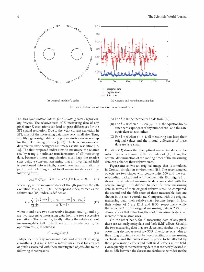

International Journal of
AerospaceEngineeringHindawi Publishing Corporationhttpwwwhindawicom Volume 2014
RoboticsJournal of
Hindawi Publishing Corporationhttpwwwhindawicom Volume 2014
Hindawi Publishing Corporationhttpwwwhindawicom Volume 2014
Active and Passive Electronic Components
Control Scienceand Engineering
Journal of
Hindawi Publishing Corporationhttpwwwhindawicom Volume 2014
International Journal of
RotatingMachinery
Hindawi Publishing Corporationhttpwwwhindawicom Volume 2014
Hindawi Publishing Corporation httpwwwhindawicom
Journal ofEngineeringVolume 2014
Submit your manuscripts athttpwwwhindawicom
VLSI Design
Hindawi Publishing Corporationhttpwwwhindawicom Volume 2014
Hindawi Publishing Corporationhttpwwwhindawicom Volume 2014
Shock and Vibration
Hindawi Publishing Corporationhttpwwwhindawicom Volume 2014
Civil EngineeringAdvances in
Acoustics and VibrationAdvances in
Hindawi Publishing Corporationhttpwwwhindawicom Volume 2014
Hindawi Publishing Corporationhttpwwwhindawicom Volume 2014
Electrical and Computer Engineering
Journal of
Advances inOptoElectronics
Hindawi Publishing Corporation httpwwwhindawicom
Volume 2014
The Scientific World JournalHindawi Publishing Corporation httpwwwhindawicom Volume 2014
SensorsJournal of
Hindawi Publishing Corporationhttpwwwhindawicom Volume 2014
Modelling amp Simulation in EngineeringHindawi Publishing Corporation httpwwwhindawicom Volume 2014
Hindawi Publishing Corporationhttpwwwhindawicom Volume 2014
Chemical EngineeringInternational Journal of Antennas and
Propagation
International Journal of
Hindawi Publishing Corporationhttpwwwhindawicom Volume 2014
Hindawi Publishing Corporationhttpwwwhindawicom Volume 2014
Navigation and Observation
International Journal of
Hindawi Publishing Corporationhttpwwwhindawicom Volume 2014
DistributedSensor Networks
International Journal of