Research Article A Methodology for Multihazards Load ...

Research ArticleA Methodology for Multihazards Load Combinations ofEarthquake and Heavy Trucks for Bridges

Dezhang Sun,1 Xu Wang,2 and Baitao Sun1

1 Department of Lifeline Engineering, Institute of Engineering Mechanics, China Earthquake Administration, Harbin 150080, China2 State Key Laboratory Breeding Base of Mountain Bridge and Tunnel Engineering, Chongqing Jiaotong University,Chongqing 400074, China

Correspondence should be addressed to Xu Wang; [email protected]

Received 2 January 2014; Accepted 15 April 2014; Published 4 May 2014

Academic Editor: Ting-Hua Yi

Copyright © 2014 Dezhang Sun et al. This is an open access article distributed under the Creative Commons Attribution License,which permits unrestricted use, distribution, and reproduction in any medium, provided the original work is properly cited.

Issues of load combinations of earthquakes and heavy trucks are important contents in multihazards bridge design. Current loadresistance factor design (LRFD) specifications usually treat extreme hazards alone and have no probabilistic basis in extreme loadcombinations. Earthquake load and heavy truck load are considered as random processes with respective characteristics, and themaximum combined load is not the simple superimposition of their maximum loads. Traditional Ferry Borges-Castaneda modelthat considers load lasting duration and occurrence probability well describes random process converting to random variables andload combinations, but this model has strict constraint in time interval selection to obtain precise results. Turkstra’s rule considersone load reaching its maximum value in bridge’s service life combined with another load with its instantaneous value (or meanvalue), which looks more rational, but the results are generally unconservative. Therefore, a modified model is presented hereconsidering both advantages of Ferry Borges-Castaneda’s model and Turkstra’s rule. The modified model is based on conditionalprobability, which can convert random process to random variables relatively easily and consider the nonmaximum factor in loadcombinations. Earthquake load and heavy truck load combinations are employed to illustrate the model. Finally, the results of anumerical simulation are used to verify the feasibility and rationality of the model.

1. Introduction

The current American bridge design specifications are main-ly based on AASHTO load and resistance factor designmethodology, which are fully calibrated against gravity loadand live load. In AASHTO LRFD bridge design specifications[1], a typical bridge is designed for 75 years’ service life andload distributions are assumed to be normal and resistance tobe lognormal. And a reliability index 3.5 is used to calibratethe safety of the bridges in strength I limit state. However,when extreme loads are considered, the sectional dimensionsand construction cost would be increased substantially ifsimilar criteria are placed [2]. Against extreme loads, eachone has its own unique approach, principally because the dataand statistics are rare. This fact makes it difficult to properlyconsider extreme loads in a consistent fashion.

In recent years, bridges are subject to more and morediversified natural hazards, and the frequencies of various

extreme hazards also seem to be increasing, which bringgreat threats to safety of the bridges so as to bring potentialdanger to personal life and property safety. The concept ofmultihazards design is quoted in many papers and reportsat present [3–7]. An organization of Multidisciplinary Centerfor Extreme Events Research (MCEER) was established, andone of the tasks is to develop a framework to systematicallyexpand the LRFD specification to multihazard (MH)-LRFDfor bridges. Many scholars and organizations have mademany studies on the effect of a single extreme load on bridge[8–11]; however, there are only a few reports of studies on theeffect of multiple extreme loads on performance of the bridgeduring its whole service life [12–14].

When there is only one extreme load (such as earth-quakes, scour, vessel collisions, etc.), the load combinationincludes an extreme load and dead load and in such caseno matter whether the extreme load is a random variableor random process, its combination only relates to the

Hindawi Publishing Corporatione Scientific World JournalVolume 2014, Article ID 126270, 9 pageshttp://dx.doi.org/10.1155/2014/126270

2 The Scientific World Journal

maximum value. It is quite a different situation when twoor more extreme loads are considered in the combinations.Because the intensity of extreme load is a function relatedto time and even two extreme loads occur simultaneously ina short time, the probability for them to reach their highestintensities at the same time is very low, which means thatwhen multiple extreme loads are combined, the maximumcombined load is not simply the superimposition of theirmaximum value. Among many load combination models,Ferry Borges-Castaneda model [15], Turkstra’s rule [16], andWen’s method [17, 18] are the most frequently used. However,they have their own advantages and disadvantages. Loadslasting duration and occurrence probability are consideredin Ferry Borges-Castaneda model, and the conversion ofrandom process to random variables and the combinationwith other random variables are well described; however,it has strict requirement for time interval. Turkstra’s ruleconsiders that a load reaches the maximum value duringdesign life of the bridge combined with the instantaneousvalue (or mean value) of another load. This rule is morepractical and reasonable, but the results are generally uncon-servative [19].Wen’s load coincidencemethod does not give arational explanation of corelation in the probability of failureof different events.

In this paper, a model based on conditional probabilityis proposed to combine advantages of the Ferry Borges-Castaneda model and Turkstra’s rule to achieve a morereasonable result of load combination. Then earthquake loadand heavy truck load combinations are employed to illustratethe model.

2. Basic Modeling

Earthquake load usually lasts for a short time and hasenormous destructive power, while the frequency of heavytrucks is relatively high and some overloaded trucks ormultiple trucks “running side by side” bring damage to thebridge greatly. It should be noticed that the maximum 75-year truck load was usually great and can be considered asextreme load. Generally, extreme load is of low occurrenceprobability and great intensity and even lower chance ofsimultaneous occurrences. Even the extreme loads do occursimultaneously; the chances that they achieve their respectivemaximum value are very low. Therefore, the common occur-rence frequencies of different extreme loads are generallynot considered [20]. According to Ferry Borges-Castanedamodel, Turkstra’s rule, and Wen’s method, it is assumed thatthe earthquake load and heavy truck load comply with stablePoisson process; the probability and times at any point of timeduring design service life of the bridge comply with Poissondistribution.The load histories of earthquake load and heavytruck load during their respective time intervals are thefunctions of time and intensity accompanied with greatrandomness, whichmakes load combination very difficult. Tosimplify the combination, it is assumed that the earthquakeand heavy truck loads maintain the maximum value duringtheir respective time history (as shown in Figure 1). Althoughsuch assumption is conservative, the problem of combination

x

T

fX(x)

X(t)

𝜏 2𝜏 3𝜏

Figure 1: Assumption of load in its duration.

T

T

T

t1

t2 t2 t2 t2 t2 t2

L1

L2

L1 + L2

Figure 2: Model of Ferry Borges-Castaneda method.

is greatly simplified. To a certain extent, “combination oftime history” is not necessarily more advantageous thanthe simplified combination because bridge design also takesthe maximum combination into consideration and it alsoincreases the level of calculation difficulty. Ferry Borges-Castaneda model that considers load lasting duration andoccurring probability well describes randomprocess convert-ing to random variables and load combinations of earthquakeand heavy truck load.Thebasic combination thought of FerryBorges-Castaneda model can be expressed as Figure 2.

Note that in Figure 1 𝑓𝑋(𝑥) is the probability density

of load in 𝜏 interval, which is the function of time andload intensity. The occurrence of load is determined throughPoisson distribution. When only two random processes areconsidered, assume that the time interval of load 1 is 𝑡

1, that

of load 2 is 𝑡2, and 𝑡

1≥ 𝑡2. Under only one kind of loads,

the maximum value of load 2 in 𝑡1interval can be described

The Scientific World Journal 3

with (1) and the maximum value of load 1 in 𝑇 period can beobtained through

𝑥max,𝑡1

= max𝑡1

[𝑥2] , (1)

𝑥max,𝑇 = max𝑇

[𝑥1] . (2)

One of the main tasks of load combination is to find themaximum value of combined load under multiple kinds ofloads in the service life of bridge. Therefore, based on theassumptions of load definition of Ferry Borges-Castanedamodel, themaximum value of load combination in 𝑡

1interval

is max (𝑥max,𝑡1

+ 𝑥1) (see Figure 2); then the maximum value

[21] in 𝑇 period can be obtained through

𝐹𝑋 max,𝑇 (𝑥) = [𝐹𝑋 (𝑥)]

𝑛, (3)

where 𝐹𝑋 max,𝑇(𝑥) is the cumulative distribution function

(CDF) of the maximum value of combined load in 𝑇period; 𝐹

𝑋(𝑥) is the cumulative distribution function of load

combination in 𝑡1interval; 𝑛 is integer, which can be obtained

from 𝑇 and 𝑡; namely, 𝑛 = 𝑇/𝑡.

3. A Modified Model for Load Combination

According to the Ferry Borges-Castaneda model, the servicelife of the bridge can be divided into equal time interval 𝑡;if it is small enough, the results are nearly precise. However,the interval of time depends on many factors; it is not smallenough and the duration of the maximum load effect of eachload within a time interval, such as heavy truck passing acommon bridge, is relatively certain, while this “duration” isusually shorter than time interval 𝑡.Therefore, the probabilityof simultaneous occurrences is not equal to the product ofrespective occurrence probabilities of the loads. If they aremade to be equal, the probability of maximum load effect isexaggerated so as to lead to conservative results. It is assumedthat the probability of occurrence probability of load 1 withininterval 𝑡 is 𝑝

1, that of load 2 is 𝑝

2, and the probability of

simultaneous occurrences is 𝑝.The probability of load 1 eventin its duration is 𝑝

1𝑟and the probability of load 2 event in its

duration is 𝑝2𝑟; then we can find

𝑝1⋅ 𝑝2̸= 𝑝1𝑟⋅ 𝑝2𝑟; 𝑝 ≥ 𝑝

1𝑟⋅ 𝑝2𝑟. (4)

Besides, power conversion of probability curves isrequired when using Ferry Borges-Castaneda model. Forexample, converting probability curve in a long time 𝑇

0to

that in an interval 𝑡, when 𝑇0≫ 𝑡, the probability curves

may have error after root of large number and the erroris cumulative, especially for curves with values on negativepart of 𝑋 axis (such as normal distribution curve). Forearthquake, annual probability curve is obtained from theUSGSMapping [22] and the computation of multiple powersfor curve conversion is needed. Therefore, the number ofpowers should be controlled to prevent loss of data becausethe number is too large.

Based on these problems, Ghosn et al. [20] improvedthe Ferry Borges-Castanedamodel.However, Ghosn believed

Heavy trucks

Heavy trucks and

earthquakes

Earthquakes

Figure 3: Illustration of heavy trucks and earthquakes sample space.

that there must be trucks on the bridge within the duration ofearthquake. This assumption is one of the important reasonscausing the conservative results of Ghosn’s model. Accordingto the report of Nowak and Szerszen [23–26], it is assumedthat it takes 8 seconds for a heavy truck to pass through acommonbridge and 600 trucks to pass through the bridge perday, and seismic excitation duration is 40 seconds. Also it isassumed that the heavy truck passing through a bridge duringthe earthquake meets the condition of Poisson process. Theeffective lasting duration of earthquake is 𝜏

𝑒and the time

for the heavy truck passing through the bridge is 𝜏𝑡; the

probability of the heavy truck on the bridge during theearthquake is 𝑃(𝑒

𝑒,tr); then,

𝑃 (𝑒𝑒,tr) ≤ 1 − 𝑒

−𝜆(𝜏𝑒+𝜏𝑡), (5)

where 𝜆 is the frequency of heavy trucks.The probability is less than 30% when (5) holds the equal

mark. Since the times of trucks passing through a commonbridge are limited in a given exposure time, the probabilityhas little change when 6 andmore trucks passing through thebridge based on Poisson distribution.

Since the number of earthquakes in a 75-year returnperiod is usually few, it is mentioned in the report of Ghosnet al. [20] that, according to USGS Mapping, the number ofearthquake in San Francisco in a 75-year return periodwill be600 and 150 in Seattle, 38 in Memphis, 30 in New York, and 1in St. Paul, which are far less than millions of heavy trucks inbridge’s service life.

The earthquake and heavy truck load combinations aredifferent from other extreme load combinations (except forscour), and the probability of simultaneous occurrences can-not be ignored just as described above. In case of earthquakeload and heavy truck load combination, the combinationsituations include heavy truck load only, heavy truck loadand earthquake load, and earthquake load only (as shownin Figure 3). If they are put together (viz., they are treatedin one sample space), the sampling probability of earthquakeis small since the number of trucks is far more than that ofearthquake; thus the most concerned probability of earth-quake effect is “very small,” which is obviously abnormal.Earthquake and heavy truck are two kinds of loads andtheir impact levels are different. In other words, althoughthe number of earthquake occurrence is less, its destructivepower and impact are larger. Besides, from a different point


Earthquake load

Heavy truck load

Load combination

t1

𝜏e

𝜏t

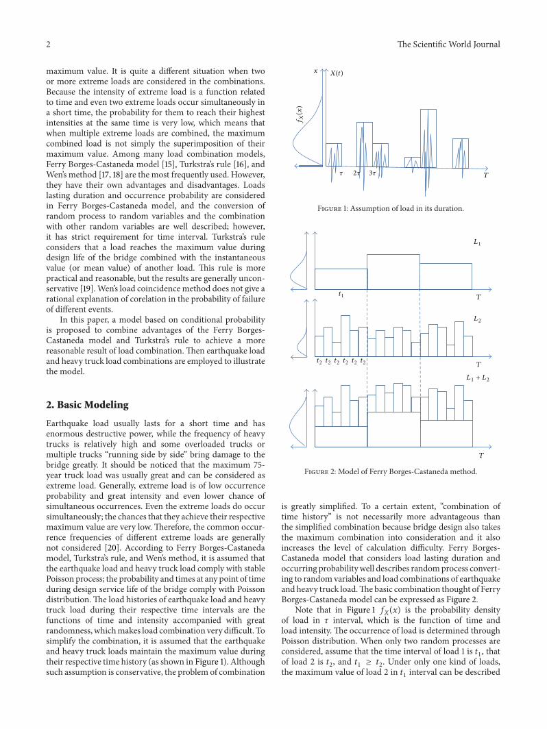
Figure 4: Illustration of load combination ofmodifiedmodel, where𝜏𝑒and 𝜏

𝑡are the event durations of earthquake and heavy truck,

respectively.

H

W

e

Figure 5: Computing model of the bridge.

of view, the probability of earthquakes to come across heavytrucks is obviously different from that of heavy trucks to comeacross earthquakes while passing the bridge. Since there aremany heavy trucks, the probability of heavy trucks to comeacross earthquakewhile passing the bridge is far less than thatof the earthquake to come across heavy trucks. For a commonbridge, the time interval for heavy trucks to cause maximumload effect is shorter than the lasting duration of earthquake.In such case, if heavy trucks are treated as the benchmark,no uniform and definite results will be obtained (becausemultiple heavy trucks may correspond to one earthquake).

To sum up, heavy trucks and earthquakes load aretwo kinds of loads with different natures and should beput in different sample spaces for their combination. Thedestructive power of earthquake is larger and the lastingduration of earthquake is longer than that of heavy truckspassing a common bridge. Therefore, it is proper to considerearthquake as the condition for load combination.

In consideration of the complexity of earthquake andheavy truck load combinations, amodifiedmodel will “inves-tigate and review” heavy trucks based on earthquake; namely,theremay be ormay not be heavy trucks on the bridge duringthe effective time interval of earthquake. If former conditionhappens, there may be multiple trucks at the same time oronly one truck, as shown in Figure 4. It is assumed that theload effect within each time 𝑡

1is independent and has the

same distribution.Analysis of the truck issues based on earthquake con-

dition will make the most concerned extreme load suchas earthquake load outstanding and clear, make load effectcombination clarified, and prevent the “confusion” whensample spaces are mixed, so as to simplify the concept of loadeffect combination. During each time 𝑡

1(a long time period),

incorporating the conception of Turkstra’s rule, the differenceis that the heavy truck load here is not instantaneous value ormean value. Since heavy truck is “observed”when earthquakehas happened, earthquake should be analyzed by numberand then earthquake and heavy truck combination couldbe considered. The expected numbers of earthquakes areprovided by USGS Mapping Project.

The cumulative distribution, 𝐹𝑒(𝑥), of load for one earth-

quake’s occurrence is defined by

𝐹𝑒 (𝑥) = [𝑃𝑦 (𝑥)]

1/𝑛𝑒𝑦

, (6)

where 𝑛𝑒𝑦is the annual average number of earthquake; 𝑃

𝑦(𝑥)

is the annual cumulative probability function curve of earth-quake load.

Note that 𝑛𝑒𝑦

may not always appear as an integer forcalculation accuracy and convenience according to differentareas and is related to total occurrence number of earthquake.

On the basis of reliability theory, combining heavy truckwith earthquake, the cumulative distribution function ofpossible maximum truck load 𝐹tr(𝑥) is calculated using thefollowing equation:

𝐹tr (𝑥) = [𝐹 (𝑥)](𝑛tr ⋅𝑛𝑒), (7)

where 𝑛tr is the quantity of heavy trucks in effective combinedaction time of earthquake and heavy trucks; 𝐹(𝑥) is the loadcumulative distribution function of a single heavy truck; 𝑛

𝑒is

the number of earthquake meeting with heavy trucks.The maximum value of combination of earthquake load

and heavy truck load is obtained through (3).The probabilityof the earthquakes “alone” (without a heavy truck passingby) is considered through the probability of earthquakeoccurrence 𝑃(𝑒only). 𝑃(𝑒𝑒,tr) is the probability of combinedaction of earthquake and heavy truck; then there is 𝑃(𝑒

𝑒,tr) +𝑃(𝑒only) = 1. Based on earthquake condition, the modifiedmodel can be expressed as

𝑃 (𝑋 ≤ 𝑥, 𝑒) = 𝑃 (𝑋 ≤ 𝑥, 𝑒𝑒,tr) + 𝑃 (𝑋 ≤ 𝑥, 𝑒𝑒,only)

= 𝑃 (𝑋 ≤ 𝑥 | 𝑒𝑒,tr) ⋅ 𝑃 (𝑒𝑒,tr)

+ 𝑃 (𝑋 ≤ 𝑥 | 𝑒𝑒,only) ⋅ 𝑃 (𝑒only)

= 𝐹𝑒,tr (𝑥) ⋅ 𝑃 (𝑒𝑒,tr) + 𝐹𝑒,only (𝑥) ⋅ 𝑃 (𝑒only) ,

(8)


0 500 1000 1500 2000 2500 30000

0.5

1

1.5

2

Intensity (kN-M)

Prob

abili

ty d

ensit

y×10−3

(a)

Intensity (kN-M)0 500 1000 1500 2000 2500 3000

0

0.5

1

1.5

Prob

abili

ty

(b)

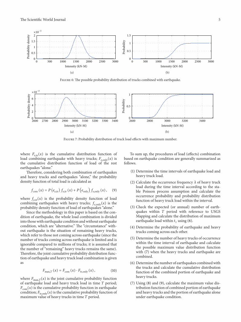
Figure 6: The possible probability distribution of trucks combined with earthquake.

2600 2700 2800 2900 3000 3100 3200 3300 34000

2

4

6

Intensity (kN-M)

Prob

abili

ty d

ensit

y

×10−3

(a)

Intensity (kN-M)2600 2800 3000 3200 34000

0.5

1

Prob

abili

ty

(b)

Figure 7: Probability distribution of truck load effects with maximum number.

where 𝐹𝑒,tr(𝑥) is the cumulative distribution function of

load combining earthquake with heavy trucks; 𝐹𝑒,only(𝑥) is

the cumulative distribution function of load of the restearthquakes “alone.”

Therefore, considering both combination of earthquakesand heavy trucks and earthquakes “alone,” the probabilitydensity function of total load is calculated as

𝑓com (𝑥) = 𝑃 (𝑒𝑒,tr) 𝑓𝑒,tr (𝑥) + 𝑃 (𝑒only) 𝑓𝑒,only (𝑥) , (9)

where 𝑓𝑒,tr(𝑥) is the probability density function of load

combining earthquakes with heavy trucks; 𝑓𝑒,only(𝑥) is the

probability density function of load of earthquakes “alone.”Since the methodology in this paper is based on the con-

dition of earthquake, the whole load combination is dividedinto thosewith earthquake condition andwithout earthquakecondition, which are “alternative.” The “circumstance” with-out earthquake is the situation of remaining heavy trucks,which refer to those not coming across earthquake (since thenumber of trucks coming across earthquake is limited and isignorable compared to millions of trucks; it is assumed thatthe number of “remaining” heavy trucks remains the same).Therefore, the joint cumulative probability distribution func-tion of earthquake and heavy truck load combination is givenas

𝐹max,𝑇 (𝑥) = 𝐹com (𝑥) ⋅ 𝐹tr,only (𝑥) , (10)

where 𝐹max,𝑇(𝑥) is the joint cumulative probability functionof earthquake load and heavy truck load in time 𝑇 period;𝐹com(𝑥) is the cumulative probability function in earthquakecondition; 𝐹tr,only(𝑥) is the cumulative probability function ofmaximum value of heavy trucks in time 𝑇 period.

To sum up, the procedures of load (effects) combinationbased on earthquake condition are generally summarized asfollows.

(1) Determine the time intervals of earthquake load andheavy truck load.

(2) Calculate the occurrence frequency 𝜆 of heavy truckload during the time interval according to the sta-ble Poisson process assumption and calculate theoccurrence probability and probability distributionfunction of heavy truck load within the interval.

(3) Check the expected (or annual) number of earth-quakes within 𝑇 period with reference to USGSMapping and calculate the distribution of maximumearthquake load within 𝑡

1using (6).

(4) Determine the probability of earthquake and heavytrucks coming across each other.

(5) Determine the number of heavy trucks of occurrencewithin the time interval of earthquake and calculatethe possible maximum value distribution functionwith (7) when the heavy trucks and earthquake arecombined.

(6) Determine the number of earthquakes combinedwiththe trucks and calculate the cumulative distributionfunction of the combined portion of earthquake andheavy trucks.

(7) Using (8) and (9), calculate the maximum value dis-tribution function of combined portion of earthquakeand heavy trucks and the portion of earthquake aloneunder earthquake condition.


0.5 1 1.5 2 2.5 30

5

10

15

Intensity (kN-M)

Prob

abili

ty d

ensit

y×10−5

×104

(a)

Intensity (kN-M)0 0.5 1 1.5 2 2.5 3

00.20.40.60.8

Cum

ulat

ive

prob

abili

ty

×104

(b)

Figure 8: Probability distribution of earthquake load effects in 75 years.

Prob

abili

ty d

ensit

y

0 0.5 1 1.5 2 2.5 30

5

10

Intensity (kN-M)

×10−5

×104

(a)

Cum

ulat

ive

prob

abili

tyIntensity (kN-M)

0 0.5 1 1.5 2 2.5 30

0.5

1

×104

(b)

Figure 9: Probability distribution of earthquake load effects alone.

(8) Calculate the final maximum value distribution using(10).

(9) If constant load effect such as dead load participatesin the combination with other load effects, it shouldbe combined with the dead load effect within 𝑇 (suchas 75 years) period.

4. Numerical Simulation and Example

In order to illustrate the feasibility and clarity of themethodology of load combination described in the precedingsection, a simple example of load combination simulation ispresented here. In order to illustrate themethod clearly, somesimplifications are made, which include the assumption thatthe earthquake load is given by𝑀 = 𝑊⋅𝐴⋅𝐻, where𝑀 is thecolumn bent moment,𝑊 is superstructure weight, 𝐴 is peakground acceleration (PGA), and 𝐻 is column calculationheight. The truck load is given by 𝑀 = 𝐹 ⋅ 𝑒, where 𝐹 isthe truck weight and 𝑒 is the eccentricity between the verticalcenter axis of the truck and the vertical axis of the column.The effects of soil and secondary effect of gravity are ignored.The computing model of the bridge is shown in Figure 5.Themain configuration of the bridge is𝑊 = 500 ton,𝐻 = 6.0m,and 𝑒 = 4m, and the bridge locates in Seattle, USA. Furtherit is assumed that the maximum number of trucks on onelane is two in one direction and in a special site heavy truckmay have an average number of 1000. Moses [27]suggestedheavy trucks approach a normal distribution with a meanof 300 kN and a standard deviation of 80 kN (coefficient ofvariable: COV=26.5%) andmore heavier truck situations canbe obtained through basic assumption above.The earthquake

curve can be found from USGS mapping, which includesPGA and frequency of exceedance and could be convertedto cumulative curve [13, 14]. According to USGS mapping,the expected number of earthquakes in Seattle is 2, and thenthere will be 150 in 75 years’ service life of common bridge.The results are given in Figure 5 to Figure 14.

According to Figures 6 and 7, the maximum truck loadcombined with earthquake is between the single commontruck load and the maximum 75-year truck load, which isreasonable because the larger the earthquake is, the smallerthe occurrence probability is and the smaller the probabilityof coming across heavier trucks will be, and, on the contrary,the smaller the earthquake is, the larger the occurrenceprobability is and the larger the probability of coming acrossheavier trucks will be.

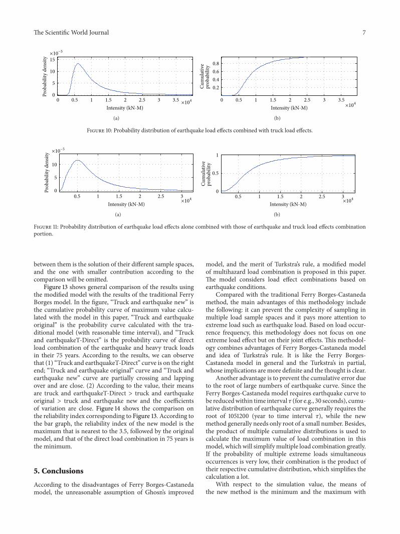
Figure 8 to Figure 12 show the results of combinationsunder earthquake condition. According to the results inFigures 9 and 10, the curves of load combinations changeafter the situation of earthquake coming across trucks isconsidered. In this example, because the probability of com-ing across between heavy trucks and earthquake is relativelysmall, we can see from the results that the shape of probabilitycurve under earthquake only is similar with that of 75 years’maximum earthquake load curve, but with the mean movingleftwards. Figure 11 shows the load combination of earth-quake load effects alone combined with those of earthquakeand truck load effects combination portion, and the result isof similar shape with the maximum earthquake load in 75years, but with the mode larger than that under earthquakeonly. Figure 12 shows the combination of the maximumload under earthquake condition and the maximum load of“remaining” heavy trucks. Consideration of the comparison


Prob

abili

ty d

ensit

y

Intensity (kN-M)0 0.5 1 1.5 2 2.5 3 3.5

0

5

10

15×10−5

×104

(a)

Cum

ulat

ive

prob

abili

ty

Intensity (kN-M)0 0.5 1 1.5 2 2.5 3 3.5

0.20.40.60.8

×104

(b)

Figure 10: Probability distribution of earthquake load effects combined with truck load effects.

Prob

abili

ty d

ensit

y

Intensity (kN-M)0.5 1 1.5 2 2.5 3

0

5

10

×10−5

×104

(a)

Cum

ulat

ive

prob

abili

ty

0.5 1 1.5 2 2.5 30

0.5

1

Intensity (kN-M) ×104

(b)

Figure 11: Probability distribution of earthquake load effects alone combined with those of earthquake and truck load effects combinationportion.

between them is the solution of their different sample spaces,and the one with smaller contribution according to thecomparison will be omitted.

Figure 13 shows general comparison of the results usingthe modified model with the results of the traditional FerryBorges model. In the figure, “Truck and earthquake new” isthe cumulative probability curve of maximum value calcu-lated with the model in this paper, “Truck and earthquakeoriginal” is the probability curve calculated with the tra-ditional model (with reasonable time interval), and “Truckand earthquakeT-Direct” is the probability curve of directload combination of the earthquake and heavy truck loadsin their 75 years. According to the results, we can observethat (1) “Truck and earthquakeT-Direct” curve is on the rightend; “Truck and earthquake original” curve and “Truck andearthquake new” curve are partially crossing and lappingover and are close. (2) According to the value, their meansare truck and earthquakeT-Direct > truck and earthquakeoriginal > truck and earthquake new and the coefficientsof variation are close. Figure 14 shows the comparison onthe reliability index corresponding to Figure 13. According tothe bar graph, the reliability index of the new model is themaximum that is nearest to the 3.5, followed by the originalmodel, and that of the direct load combination in 75 years isthe minimum.

5. Conclusions

According to the disadvantages of Ferry Borges-Castanedamodel, the unreasonable assumption of Ghosn’s improved

model, and the merit of Turkstra’s rule, a modified modelof multihazard load combination is proposed in this paper.The model considers load effect combinations based onearthquake conditions.

Compared with the traditional Ferry Borges-Castanedamethod, the main advantages of this methodology includethe following: it can prevent the complexity of sampling inmultiple load sample spaces and it pays more attention toextreme load such as earthquake load. Based on load occur-rence frequency, this methodology does not focus on oneextreme load effect but on their joint effects. This methodol-ogy combines advantages of Ferry Borges-Castaneda modeland idea of Turkstra’s rule. It is like the Ferry Borges-Castaneda model in general and the Turkstra’s in partial,whose implications are more definite and the thought is clear.

Another advantage is to prevent the cumulative error dueto the root of large numbers of earthquake curve. Since theFerry Borges-Castaneda model requires earthquake curve tobe reducedwithin time interval 𝜏 (for e.g., 30 seconds), cumu-lative distribution of earthquake curve generally requires theroot of 1051200 (year to time interval 𝜏), while the newmethod generally needs only root of a small number. Besides,the product of multiple cumulative distributions is used tocalculate the maximum value of load combination in thismodel, whichwill simplifymultiple load combination greatly.If the probability of multiple extreme loads simultaneousoccurrences is very low, their combination is the product oftheir respective cumulative distribution, which simplifies thecalculation a lot.

With respect to the simulation value, the means ofthe new method is the minimum and the maximum with

8 The Scientific World JournalPr

obab

ility

den

sity

0 0.5 1 1.5 2 2.5 3 3.5 4

12345×10−4


(a)

Cum

ulat

ive

prob

abili

ty

0.5 1 1.5 2 2.5 3 3.5 40

0.20.40.60.8


(b)

Figure 12: Probability distribution of load effects under earthquake condition combined with remaining truck load effects in 75 years.

0 2 4 6 8 100

0.1

0.2

0.3

0.4

0.5

0.6

0.7

0.8

0.9

1

Cum

ulat

ive p

roba

bilit

y

Truck and earthquake newTruck and earthquake originalTruck and earthquake T-Direct


Figure 13: Comparison of cumulative probability curves withdifferent methods.

3.153.2

3.253.3

3.353.4

3.453.5

Beta new Beta ogi Beta-dic

Figure 14: Comparison of reliability index corresponding to thecurves in Figure 13.

reliability index, while the value of combination in 𝑇 periodis the most conservative. Furthermore, the results of differentregions may be different because the earthquakes of thechosen regions are greatly different. For example, earthquakesin California are frequent, and thus the load combination is

greatly affected by earthquake. Earthquakes in St. Paul are lessfrequent, and thus the impact is mainly from the trucks. ForNew York, the impacts from neither earthquake nor truckscan be ignored and the participation of earthquake and heavytrucks in the results is approximate.

Conflict of Interests

The authors declare that there is no conflict of interestsregarding the publication of this paper.

Acknowledgments

This study is jointly funded by Institute Basic ScientificResearch Fund (Grant no. 2012A02), the National NaturalScience Fund of China (NSFC) (Grant no. 51308510), OpenFund of State Key Laboratory Breeding Base of MountainBridge and Tunnel Engineering (Grant no. CQSLBF-Y14-15),and Zhejiang Provincial Natural Science Foundation (Grantno. Q12E080026). The results and conclusions presented inthe paper are related to the authors and do not necessarilyreflect the view of the sponsors.

References

[1] AASHTO Guide Specification for LRFD Seismic Bridge Design,AASHTO, Washington, DC, USA, 6th edition, 2012.

[2] S. E. Hida, “Statistical significance of less common load combi-nations,” Journal of Bridge Engineering, vol. 12, no. 3, pp. 389–393, 2007.

[3] B. R. Ellingwood, “Load and resistance factor criteria forprogressive collapse design,” in Proceedings of the NationalWorkshop on Prevention of Progressive Collapse, MultihazardMitigation Council of the National Institute of Building Sci-ences, Rosemont, Ill, USA, 2002.

[4] F. A. Potra and E. Simiu, “Multihazard design: structuraloptimization approach,” Journal of Optimization Theory andApplications, vol. 144, no. 1, pp. 120–136, 2010.

[5] C. Crosti, D. Duthinh, and E. Simiu, “Risk consistency andsynergy in multihazard design,” ASCE Journal of StructuralEngineering, vol. 137, no. 8, pp. 844–849, 2011.

[6] Y. Li and B. R. Ellingwood, “Framework for multihazardrisk assessment and mitigation for wood-frame residentialconstruction,” ASCE Journal of Structural Engineering, vol. 135,no. 2, pp. 159–168, 2009.


[7] Y. Li, A. Ahuja, and J. E. Padgett, “Review of methods toassess, design for, and mitigate multiple hazards,” Journal ofPerformance of Constructed Facilities, vol. 26, no. 1, pp. 104–117,2012.

[8] B. G. Nielson and R. DesRoches, “Analytical seismic fragilitycurves for typical bridges in the central and southeasternUnitedStates,” Earthquake Spectra, vol. 23, no. 3, pp. 615–633, 2007.

[9] H. Li, T. Yi, M. Gu, and L. Huo, “Evaluation of earthquake-induced structural damages by wavelet transform,” Progress inNatural Science, vol. 19, no. 4, pp. 461–470, 2009.

[10] T. H. Yi, H. N. Li, and M. Gu, “Wavelet based multi-stepfiltering method for bridge health monitoring using GPS andaccelerometer,” Smart Structures and Systems, vol. 11, no. 4, pp.331–348, 2013.

[11] T. H. Yi, H. N. Li, and M. Gu, “Experimental assessment ofhigh-rate GPS receivers for deformation monitoring of bridge,”Measurement, vol. 46, no. 1, pp. 420–432, 2013.

[12] D. Duthinh and E. Simiu, “Safety of structures in strong windsand earthquakes: multihazard considerations,” ASCE Journal ofStructural Engineering, vol. 136, no. 3, pp. 330–333, 2010.

[13] Z. Liang and G. C. Lee, “Towards multiple hazard resilientbridges: a methodology for modeling frequent and infrequenttime-varying loads. Part I: comprehensive reliability and partialfailure probabilities,” Earthquake Engineering and EngineeringVibration, vol. 11, no. 3, pp. 293–301, 2012.

[14] Z. Liang and G. C. Lee, “Towards multiple hazard resilientbridges: a methodology for modeling frequent and infrequenttime-varying loads. Part II: examples for live and earthquakeload effects,”Earthquake Engineering and EngineeringVibration,vol. 11, no. 3, pp. 303–311, 2012.

[15] “Probabilistic design of reinforced concrete buildings,” ACIPublication SP-31, American Concrete Institute, Detroit, Mich,USA, 1971.

[16] C. J. Turkstra and H. O. Madsen, “Load combinations in codi-fied structural design,” ASCE Journal of Structural Engineering,vol. 106, no. 12, pp. 2527–2543, 1980.

[17] Y.-K. Wen, “Statistical combination of extreme loads,” ASCEJournal of Structural Engineering, vol. 103, no. 5, pp. 1079–1093,1977.

[18] Y.-K. Wen, “Clustering model for correlated load processes,”ASCE Journal of Structural Engineering, vol. 107, no. 5, pp. 965–983, 1981.

[19] E. Miranda, “Strength reduction factors in performance-baseddesign,” in Proceedings of the EERC-CUREe Symposium inHonor of Vitelmo V. Bertero, Berkeley, Calif, USA, 1997.

[20] M. Ghosn, F. Moses, and J. Wang, “Design of highway bridgesfor extreme events,” Transportation Research Board NCHRP489, National Research Council, Washington, DC, USA, 2003.

[21] T. T. Soong, Fundamentals of Probability and Statistics forEngineers, State University of New York at Buffalo, Buffalo, NY,USA, 2004.

[22] D. Z. Sun, B. T. Sun, and G. C. Lee, “Study on the combinationof earthquake and heavy trucks to bridge based on Ferry BorgesTheory,”Earthquake Engineering and EngineeringVibration, vol.31, no. 6, pp. 8–13, 2011 (Chinese).

[23] A. S. Nowak, “Calibration of LRFD bridge design code,”Transportation Research Board NCHRP Report 368, NationalAcademies, Washington, DC, USA, 1999.

[24] A. S. Nowak and M. M. Szerszen, “Structural reliability asapplied to highway bridges,” Progress in Structural Engineeringand Materials, vol. 2, pp. 218–224, 2000.

[25] A. S. Nowak and M. M. Szerszen, “Bridge load and resistancemodels,” Engineering Structures, vol. 20, no. 11, pp. 985–990,1998.

[26] A. S. Nowak, “System reliability models for bridge structures,”Bulletin of the Polish Academy of Sciences: Technical Sciences, vol.52, no. 4, pp. 321–328, 2004.

[27] F. Moses, “Calibration of load factors for LRFD bridge eval-uations,” Transportation Research Board NCHRP Report 454,National Academies, Washington, DC, USA, 2001.

International Journal of

AerospaceEngineeringHindawi Publishing Corporationhttp://www.hindawi.com Volume 2014

RoboticsJournal of

Hindawi Publishing Corporationhttp://www.hindawi.com Volume 2014


Active and Passive Electronic Components

Control Scienceand Engineering

Journal of



RotatingMachinery


Hindawi Publishing Corporation http://www.hindawi.com

Journal ofEngineeringVolume 2014

Submit your manuscripts athttp://www.hindawi.com

VLSI Design



Shock and Vibration


Civil EngineeringAdvances in

Acoustics and VibrationAdvances in



Electrical and Computer Engineering

Journal of

Advances inOptoElectronics

Hindawi Publishing Corporation http://www.hindawi.com

Volume 2014

The Scientific World JournalHindawi Publishing Corporation http://www.hindawi.com Volume 2014

SensorsJournal of


Modelling & Simulation in EngineeringHindawi Publishing Corporation http://www.hindawi.com Volume 2014


Chemical EngineeringInternational Journal of Antennas and

Propagation




Navigation and Observation



DistributedSensor Networks


Research Article A Methodology for Multihazards Load ...

Documents

Transcript of Research Article A Methodology for Multihazards Load ...