Resale Price Maintenance in an Oligopoly with Uncertain...

1

Resale Price Maintenance in an Oligopoly with

Uncertain Demand*

Hao Wang**

Department of Economics

The Ohio State University

August 2001

This paper tries to clarify the effects of resale price maintenance (RPM) in a market where

there is demand uncertainty and the manufacturers have to compete with one another. It shows

that with RPM, competing manufacturers can earn more profits, promote wholesale demand for

inventories from the retailers, enhance the social welfare, and preclude the possible coordination

failure between the manufacturers. But the effect of RPM on the consumer surplus is ambiguous.

Key Words: RPM, Demand uncertainty, Oligopoly

JEL Classification Code: L1, L4, M3

* I am grateful to Professor James Peck and Howard Marvel for their help in writing this paper. I also thank Professor Andrew Ching and Dan Levin for useful suggestions. All errors are mine. ** Corresponding Address: Department of Economics, The Ohio State University, 410 Arps Hall, 1945 North High Street, Columbus, OH 43210. Tel: (614)688-9031. Fax: (614)292-3906. E-mail: [email protected].

2

I. Introduction

This paper intends to clarify the effects of strategic interaction among the manufacturers on

the advantages of resale price maintenance (RPM) in a market with demand uncertainty.

Particularly, it focuses on the impact of RPM on the manufacturers’ profits, consumer surplus,

and social welfare. In the model, the oligopolistic manufacturers sell their products to the

consumers through competitive retailers in a marketplace where the number of consumers in the

market is a random variable. This paper considers the games without and with resale price

maintenance and then observes the difference brought by RPM. The games defined in this paper

significantly differ from those in previous works by modeling the strategic interaction between

the manufacturers.

RPM has been a contentious topic in the industrial organization literature for decades.

Different theories have been developed to address this behavior of manufacturing firms. One line

of justifications is the free riding theories represented by Telser [1960]. The free riding theories

assume that the demand for a manufacturer’s product depends on some informational services

provided by the retailers. RPM enables the retailers to capture the demand generated by the

services and thus provides incentive for them to invest in those services. RPM then improves

social efficiency by enhancing demand. However, new theory is needed to justify the use of RPM

for the products that do not need extensive sale services. Deneckere, Marvel and Peck [1996,

1997] explain the RPM use from another standpoint. They find that a manufacturer facing

uncertain demand has an incentive to support adequate retail inventories by preventing the

emergence of discount retailers. They analyze a model with a monopoly manufacturer selling to

competitive retailers in a market where the demand is uncertain. They find that with RPM, the

monopoly manufacturer has higher wholesale demand and makes more profits.

The results reported by Deneckere, Marvel and Peck are impressive. However, the results are

based on the analysis of a model with a monopoly manufacturer, which is restrictive. In the real

life, RPM or its equivalent programs are more frequently observed in markets with inter-

manufacturer competition. It is unclear whether the incentive that works in a monopoly still

3

works in an oligopoly. Thus some issues (especially some anti-trust issues) cannot be addressed

satisfactorily without a theory capable of extending those results on RPM to markets where the

manufacturers have to compete with each other.

The competition among the manufacturers adds another layer of complication to the model

considered by Deneckere, Marvel and Peck [1996]. In a monopoly, the retailers’ behaviors are

simply determined by the manufacturer’s wholesale price. But in an oligopoly, the manufacturers

have to anticipate the strategic interaction among the retailers before choosing their own

strategies. However, if the demand is uncertain, as the price dispersion found in a monopoly

(Prescott [1975], Bryant [1980], Eden [1990]), this paper finds that in an oligopoly, the entire set

of retail prices of each manufacturer’s product is still solely determined by that manufacturer’s

wholesale price, which makes the model tractable. However, the retail inventories are now

determined by both manufacturers’ wholesale prices. This paper also finds that RPM encourages

the retailers to stock greater inventories, even when the manufacturers have to compete with one

another. The manufacturers thus enhance the retailers' expected sale and make more profits.

Under the assumption that the demand is either high or low, the game without RPM can result in

two types of symmetric equilibria: low wholesale price equilibrium and high wholesale price

equilibrium. And it is possible for the game to have the two types of equilibria simultaneously. In

this case, high wholesale price equilibrium represents a high level of coordination between the

manufacturers. It results in high profits for the manufacturers but low consumer surplus. On the

contrary, the low wholesale price equilibrium represents a coordination failure. However, if RPM

is allowed, the possibility of coordination failure is ruled out. Our model makes it easy to discuss

welfare issues since the consumers have unit demand, though there is product differentiation in

the model. RPM can enhance the social welfare by encouraging the retailers to stock greater

inventories and thus facilitating greater expected sales to the consumers. RPM can also transfer

some benefits from the consumers to the manufacturers, because the average retail prices are not

lower under RPM. The consumers as a whole can be better off if significantly more consumers

are served under RPM. Otherwise they are worse off with RPM. The advantages of RPM found

4

by Deneckere, Marvel and Peck [1996] in markets with demand uncertainty are well preserved

even if the strategic interaction between the manufacturers is taken into consideration.

This paper will advance as follows. Section II depicts the model and the definitions of the

games. Sections III and IV analyze and solve for the subgame perfect Nash equilibria of the

games. The welfare issues are addressed in section V. Section VI discusses an example about the

recent use of Minimum Advertised Price (MAP) programs in prerecorded music market. Some

summary remarks are given in section VII. The Appendix provides the proofs of the three

propositions in Section III.

II. The Model

The market and the games

This is a symmetric model with duopoly manufacturers and competitive retailers. The two

manufacturers are denoted by 0 and 1. They produce horizontally differentiated, non-storable

products. The manufacturers have identical cost functions, which are assumed to be zero1. The

feasible specifications of the goods are normalized to interval [0,1]. Assume the specification of

manufacturer 0’s product is 0 and that of manufacturer 1’s product is 1.

The consumers have unit demand. It is common knowledge that the consumers’ most

preferred specifications are evenly distributed along [0, 1]. But each particular consumer’s taste is

private information. If a consumer’s most preferred specification is x , the consumer’s utility

from consuming manufacturer 0’s product is tx−1 and the utility from consuming manufacturer

1’s product is )1(1 xt −− . Parameter t represents the degree of product differentiation.

The market demand is uncertain. The measure of active consumers θ is a random variable

and iiiprob ααθθ −== +1}{ , for },...,2,1{ ni ∈ , where 1...0 21 =<<<≤ nθθθ and

1 The results of this paper remain valid with positive marginal costs c>0.

5

1...0 121 =<<<<= +nn αααα . We can define demand pocket i as the portion of demand that

would show up in the market if and only if iθθ ≥ .2 Therefore we have n demand pockets

denoted as n,...,2,1 . The measure of demand pocket i is 1−− ii θθ (let 00 =θ ). The demand

pocket i ’s probability of entering the market is iα−1 because iiprob αθθ −=≥ 1}{ . The

consumers’ probabilities of entering the market are independent to the consumers’ preferences.

The retail market is perfectly competitive. The retailers have zero dealing costs. Unsold retail

inventories cannot be returned to the manufacturers. Without loss of generality, we adopt the

convention that every retailer carries only one manufacturer’s product and charges a single price.3

From the paper by Deneckere, Marvel and Peck [1996], each manufacturer should always

prefer to use RPM, given the other manufacturer’s strategy. Thus this paper only defines two

games depending on whether RPM is allowed: the niche competition game and the RPM game.4

The niche competition game: First, the two manufacturers simultaneously announce their

wholesale prices. Second, the retailers order inventories from the manufacturers and decide the

retail prices. Third, the demand uncertainty resolves and the consumers come to the market. The

2 If iθθ ≥ , the consumers in the market can be represented by interval [0, iθ ]. If iθθ < , the

consumers NOT in the market can be represented by interval [ 1−iθ , 1]. Therefore the consumers

in the market if and only if iθθ ≥ is [ 1−iθ , iθ ], whose measure is 1−− ii θθ .

3 As long as the retailers are perfectly competitive, every single unit of retail inventory with a

price tag on it should yield zero expected profit for the retailer who carries that unit. Assuming a

retailer can carry both manufacturers’ products and charge multiple prices would not affect the

price-inventory configuration in equilibrium. Therefore it would not change any result of this

paper except requiring more notations.

4 The rationing rule employed in the games is first-come-first-served.

6

consumers enter the market sequentially in random order. Each active consumer chooses a

retailer to purchase such that his/her utility is maximized.

The RPM game: First, the two manufacturers simultaneously announce their wholesale

prices and retail prices. Second, the retailers order inventories from the manufacturers. Third,

the demand uncertainty resolves and the consumers come to the market. The consumers enter the

market sequentially in random order. Each active consumer chooses a retailer to purchase such

that his/her utility is maximized. Since a unique price is charged for each manufacturer’s

product, I assume the ratios of sale to inventory are identical for all retailers selling the same

product.

A note on the model with certain demand

As a benchmark, consider the price competition game played by two vertically integrated

manufacturers, where the market demand is certain. Suppose there is a continuum of consumers

with measure of 1. Denote the prices as 0p and 1p . Let 10 ≤p and 11 ≤p since the consumers’

reservation prices are not greater than 1. There are three possible types of symmetric equilibria

for this game, depending on the degree to which the manufacturers’ products are differentiated.

1. Typical Oligopoly: If 32<t , the equilibrium prices are tpp == *

1*0 (See Tirole [1988] for

details). In this equilibrium, the manufacturers compete at the margin and all active consumers

receive positive consumer surplus. A result that can apply to all games defined in this paper is

Lemma 2.1 If the retail prices 0p and 1p satisfy | 10 pp − | t≤ , then all consumers are served

by the manufacturers if and only if tpp −≤+ 210 .

Proof: The consumer that is least likely to purchase the product is the “marginal consumer”

who is indifferent between purchasing from either manufacturer. Denoting the marginal

7

consumer's most preferred specification as x , it should satisfy )1(10 xtptxp −+=+ . Hence

21

201 +−=

tpp

x . But 10 ≤≤ x if and only if | 10 pp − | t≤ . The marginal consumer would

purchase the product if and only if 1)21

2( 0

01 ≤++−pt

tpp

, which is equivalent to

tpp −≤+ 210 . Q.E.D.

2. Restricted oligopoly: If 132 ≤≤ t , the equilibrium prices are

21*

1*0

tpp −== . In this case

the manufacturers still interact with each other, but the competition is limited. Given 2

10

tp −= ,

manufacturer 1 faces a demand curve with a kink point at 2

1t− : If

211

tp −< , the

manufacturers compete at the margin since tpp −<+ 210 (Lemma 2.1). Thus the demand

function would be 21

210

1 +−=tpp

x . If 2

11

tp −> , the manufacturers do not compete with each

other since tpp −>+ 210 . Thus the demand function would be t

px 1

1

1−= . Both

manufacturers choose price 2

1t− in equilibrium when 1

32 ≤< t , and the marginal consumer

receives zero surplus.

3. Monopoly : If t >1, the equilibrium prices are 21*

1*0 == pp . The market is segmented into

two monopoly markets.

8

III. The Niche Competition Game

In this section we will find the subgame perfect Nash equilibrium of the niche competition

game. We solve the retailers’ subgame first, then solve the manufacturers’ problems. In order to

focus on the oligopoly situations, we assume 32

0 <≤ t from now on.

The retailers’ subgame

In the niche competition game, the wholesale prices, denoted as 0w and 1w , are exogenous to

the retailers. Lemma 3.1 characterizes the equilibrium of the retailers’ subgame. An important

characteristic of the equilibrium configuration of the niche competition game derived from

Lemma 3.1 is presented in Proposition 3.2.

Lemma 3.1 In the niche competition game, the retailers’ subgame has a unique equilibrium

configuration of prices and quantities. In that equilibrium configuration, there is a group of

retailers catering to each demand pocket. The retailers catering to demand pocket i charge retail

price of i

w

α−10 or

i

w

α−11 , and stock the pre-sale total inventories (denoted as iI0 and iI1 ) that

are exactly enough to serve demand pocket i at those retail prices. 5

5 Inventories iI0 and iI1 can be uniquely determined given 0w and 1w . But explicitly specifying

them is very complex for arbitrary 0w and 1w . Essentially, we find the measure of consumers in

demand pocket 1 who can to purchase from each manufacturer at prices 0w and 1w . Next, we

find the measure of consumers in demand pockets 1 and 2 who are not able to purchase at prices

0w and 1w , but wish to purchase at prices )1/( 10 α−w and )1/( 11 α−w . Iterating this

procedure yields iI0 and iI1 . We omit the details.

9

Proof: According to the rules of the game and the price configuration depicted in the lemma,

for any },...,2,1{ ni ∈ , the retailers charging retail price i

w

α−10 or

i

w

α−11 can sell their

inventories with probability of iα−1 (when iθθ ≥ ). So they earn zero profits. This price

configuration is an equilibrium because any deviation by any single retailer would not be

profitable: raising its price leads to a loss because of lower probability of selling; lowering its

price also leads to a loss because of less revenue from sale.

Now we show that any departure from the configuration stated in the lemma cannot be an

equilibrium. First, apparently no retailer would charge retail price lower than the wholesale price

0w (or 1w ) in equilibrium. Second, if the retail inventory at 0w (or 1w ) is not 10I (or 1

1I ), the

configuration cannot be an equilibrium because: if the total retail inventory at 0w (or 1w ) is

greater than 10I (or 1

1I ), the retailers cannot break even because its probability of selling is less

than 11 1 =−α ; if the total retail inventory at 0w (or 1w ) is less than 10I (or 1

1I ), the residual

demand can be profitably served by a retailer charging ε+0w (for small ε ). Third, any retailer

charging a price between 1

0

1 α−w

and 2

0

1 α−w

(or a price between 1

1

1 α−w

and 2

1

1 α−w

) cannot

break even, because they can only sell their inventories with probability of 21 α− (note that

demand pocket 1 is served by retailers charging 0w and 1w ). Iterating the reasoning of the

second and third steps, we can see that for any },...,3,2{ ni ∈ , if the retail inventory at i

w

α−10 (or

i

w

α−11 ) is not iI0 (or iI1 ), the configuration cannot be an equilibrium. And any retailer charging a

price between i

w

α−10 and

1

0

1 +− i

w

α (or between

i

w

α−11 and

1

1

1 +− i

w

α) cannot break even. Thus

the configuration stated in the lemma is the unique equilibrium configuration of the retailers’

subgame. Q.E.D.

10

Proposition 3.2 In the niche competition game, the retail prices of a manufacturer's product

only depend on the wholesale price of that manufacturer.

Lemma 3.1 says that the price that a competitive retailer charges depends on the probability

of selling. For instance, if a retailer expects its inventory to be sold with probability of 0.5, then

this retailer would charge retail price that is twice as much as the wholesale price in order to

break even. Introducing the competition by manufacturers into the model complicates the

retailers’ subgame because the retailers now face inter-brand competition as well as intra-brand

competition. Proposition 3.2 points out that the whole set of retail prices of a manufacturer’s

product is still solely determined by the manufacturer’s wholesale price, but not affected by its

rival’s behavior. In other words, the retail prices in this oligopoly game are still determined by the

intra-brand competition in the same way as that in a monopoly. However, the retailers’ pre-sale

inventories are now determined by both manufacturers’ wholesale prices. The inter-brand

competition only influences the retailers’ inventory decisions, but not their pricing decisions. This

proposition also makes the manufacturers’ problem tractable.

The manufacturers’ problem

Each manufacturer, anticipating the ensuing retailer’s subgame, chooses its optimal reacting

wholesale price 0w or 1w to maximize its profit. The manufacturers’ profits are simply their

wholesale revenues since the production is costless. Unfortunately, even with the relief brought

by Proposition 3.2, solving the manufacturers’ problem in a general model is still exceptionally

difficult because too many situations could arise. We will consider a simplified model where the

demand is either low or high. The measure of active consumers is 5.0 in the low demand and 1

in the high demand. Assume qprob == )5.0(θ and qprob −== 1)1(θ . Hence we have two

demand pockets, denoted by 1 and 2. Each demand pocket has the size of 0.5. Demand pocket 1

enters the market with probability of 1 and pocket 2 enters with probability of q−1 .

11

We only consider the symmetric equilibria in order to compare them to the equilibrium of the

RPM game, which is always symmetric. The following strategy is used to locate the equilibria of

the niche competition game. First, assume the symmetric equilibrium wholesale prices are in a

certain interval so that the manufacturers’ profit functions can be identified. Second, solve for the

corresponding candidate equilibrium prices. At last, characterize the necessary and sufficient

conditions under which the manufacturers cannot profitably deviate from the candidate

equilibrium prices. There are many potential types of equilibrium. In particular, for each niche,

competition can be characterized as “typical oligopoly” where the marginal consumer of the

demand pocket receives surplus; “restricted oligopoly” where the marginal consumer receives no

surplus yet the demand pocket is fully served; “monopoly” where the demand pocket is partially

served; and the case in which the demand pocket is not served at all. However, it turns out that

only three types of equilibria can actually occur, as shown by the following lemma.

Lemma 3.3 In the niche competition game, the equilibrium can only take three types:

Type I. ))1)(2

1(,0(, *1

*0 q

tww −−∈ .

Type II. )1)(2

1(*1

*0 q

tww −−== .

Type III. )2

1,1(, *1

*0

tqww −−∈ , (when qt 2< ).

Proof. (See the Appendix)

The proof of Lemma 3.3 is put in the Appendix. Types I, II and III equilibria are

characterized in the following Propositions 3.4, 3.5 and 3.6 respectively. In type I equilibrium, the

manufacturers compete at the margin in both demand pockets because tq

w

q

w −<−

+−

211

*1

*0

(Lemma 2.1) and all active consumers receive positive surplus. In type II equilibrium, both

12

demand pockets are fully served but the competition between the manufacturers is limited in

demand pocket 2. In type III equilibrium, demand pocket 1 is fully served, but pocket 2 is not

served at all. The proofs of the following propositions are put in the Appendix.

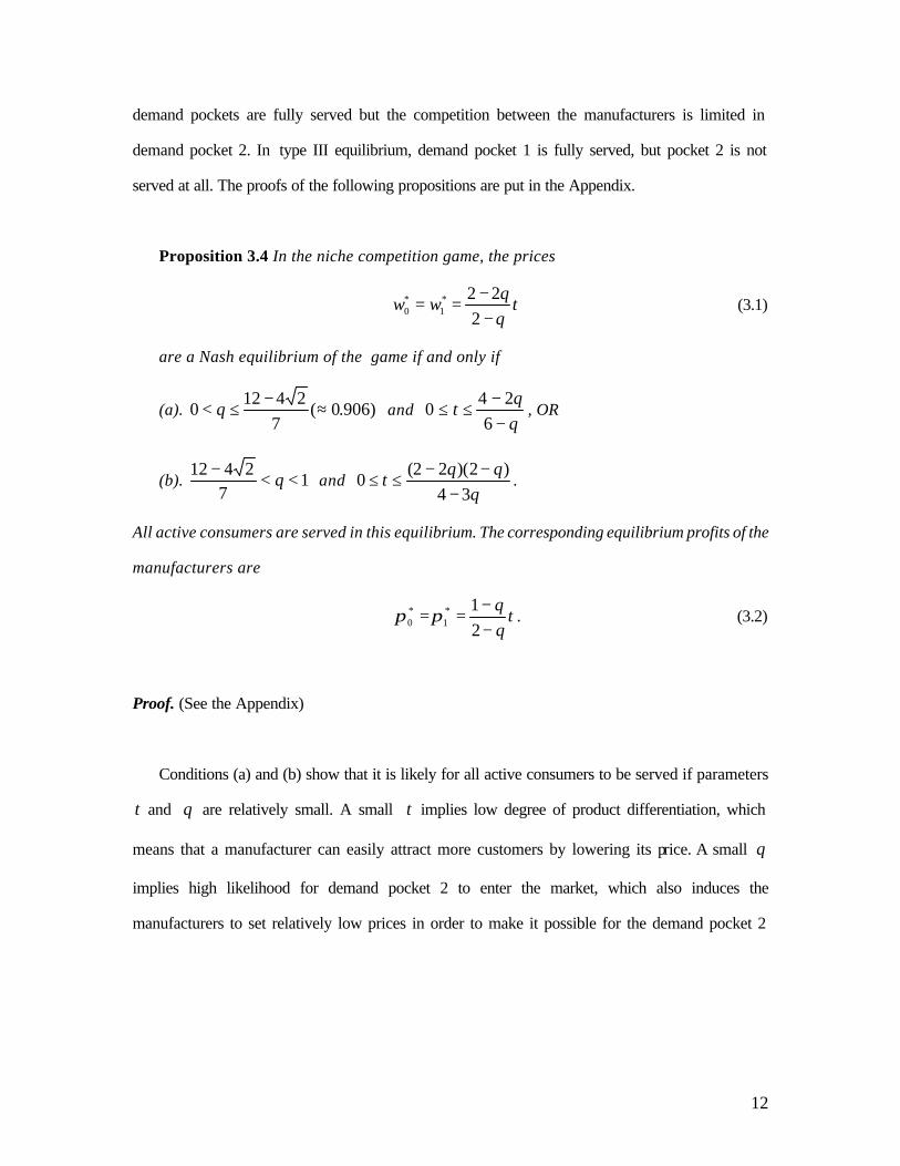
Proposition 3.4 In the niche competition game, the prices

tq

qww

−−==

222*

1*0 (3.1)

are a Nash equilibrium of the game if and only if

(a). )906.0(7

24120 ≈−≤< q and

q

qt

−−≤≤

624

0 , OR

(b). 17

2412 <<−q and

q

qqt

34)2)(22(

0−

−−≤≤ .

All active consumers are served in this equilibrium. The corresponding equilibrium profits of the

manufacturers are

tq

q

−−==

21*

1*0 ππ . (3.2)


Conditions (a) and (b) show that it is likely for all active consumers to be served if parameters

t and q are relatively small. A small t implies low degree of product differentiation, which

means that a manufacturer can easily attract more customers by lowering its price. A small q

implies high likelihood for demand pocket 2 to enter the market, which also induces the

manufacturers to set relatively low prices in order to make it possible for the demand pocket 2

13

getting served. The gray area in Figure6 3.1, called area 1, illustrates the set of parameters ),( tq

satisfying condition (a) or (b).

0.2 0.4 0.6 0.8 1 q 0.1 0.2 0.3 0.4 0.5 0.6

t

0.2 0.4 0.6 0.8 1 q 0.1 0.2 0.3 0.4 0.5 0.6

t

Figure 3.1


)1)(2

1(*1

*0 q

tww −−== (3.3)


(c). q

qt

q

q

−−−≤≤

−−

247

226

24.


manufacturers are

)1)(2

1(21*

1*0 q

t −−== ππ . (3.4)


Figure 3.2 shows the set of parameters ),( tq that satisfy condition (c), called area 2, and thus

supports type II equilibrium.

6 The figures in this paper are created in Mathematica 4, Wolfram Research [1999].

14

0.2 0.4 0.6 0.8 1 q 0.1 0.2 0.3 0.4 0.5 0.6

t

0.2 0.4 0.6 0.8 1 q 0.1 0.2 0.3 0.4 0.5 0.6

t

Figure 3.2


tww == *1

*0 (3.5)


(d). )366.0(2

310 ≈+−≤≤ t and 1

1)33(1 <≤

−−−

qt

t, OR

(e). 32

231 <<+−

t and 121

21

2

<≤+

− qt

t.

Only demand pocket 1 is served in this equilibrium. The corresponding equilibrium profits of the

manufacturers are

4*1

*0

t==ππ . (3.6)


Type III equilibrium is likely to occur with relatively great parameter t and q , which imply

that the product differentiation is significant and demand pocket 2 is unlikely to enter the market.

Therefore the manufacturers are likely to give up demand pocket 2 and serve pocket 1 only. Type

III equilibrium is not Pareto efficient because some consumers are not served though they have

15

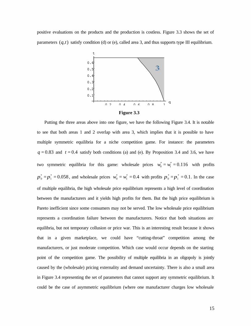
positive evaluations on the products and the production is costless. Figure 3.3 shows the set of

parameters ),( tq satisfy condition (d) or (e), called area 3, and thus supports type III equilibrium.

0.2 0.4 0.6 0.8 1 q 0.1 0.2 0.3 0.4 0.5 0.6

t

0.2 0.4 0.6 0.8 1 q 0.1 0.2 0.3 0.4 0.5 0.6

t

Figure 3.3

Putting the three areas above into one figure, we have the following Figure 3.4. It is notable

to see that both areas 1 and 2 overlap with area 3, which implies that it is possible to have

multiple symmetric equilibria for a niche competition game. For instance: the parameters

83.0=q and 4.0=t satisfy both conditions (a) and (e). By Proposition 3.4 and 3.6, we have

two symmetric equilibria for this game: wholesale prices 116.0*1

*0 == ww with profits

058.0*1

*0 ==ππ , and wholesale prices 4.0*

1*0 == ww with profits 1.0*

1*0 ==ππ . In the case

of multiple equilibria, the high wholesale price equilibrium represents a high level of coordination

between the manufacturers and it yields high profits for them. But the high price equilibrium is

Pareto inefficient since some consumers may not be served. The low wholesale price equilibrium

represents a coordination failure between the manufacturers. Notice that both situations are

equilibria, but not temporary collusion or price war. This is an interesting result because it shows

that in a given marketplace, we could have “cutting-throat” competition among the

manufacturers, or just moderate competition. Which case would occur depends on the starting

point of the competition game. The possibility of multiple equilibria in an oligopoly is jointly

caused by the (wholesale) pricing externality and demand uncertainty. There is also a small area

in Figure 3.4 representing the set of parameters that cannot support any symmetric equilibrium. It

could be the case of asymmetric equilibrium (where one manufacturer charges low wholesale

16

price and serve both demand pockets and another manufacturer charges high price and serve

demand pocket 1 only), or no equilibrium at all.

0.2 0.4 0.6 0.8 1q

0.1

0.2

0.3

0.4

0.5

0.6

t

0.2 0.4 0.6 0.8 1q

0.1

0.2

0.3

0.4

0.5

0.6

t

Figure 3.4

IV. The RPM Game

The retailers’ subgame

In the RPM game, the manufacturers specify both the wholesale prices and retail prices. The

retailers only decide how much inventory to order. The retailers can earn a margin from sale, but

the competition drives the retailers’ inventories to be higher than their expected sales. Therefore

they still make zero profits in equilibrium. The following lemma characterizes the equilibrium of

the retailers’ subgame.

Lemma 4.1 In the equilibrium of the retailers’ subgame in the RPM game, the ratio of a

retailer’s inventory to its expected sale equals the manufacturer’s retail price markup.

Proof: Without loss of generality, consider manufacturer 0 only. Denote: 0w wholesale

price of manufacturer 0, 0r retail price of manufacturer 0, 0d expected sale of a retailer

dealing manufacturer 0’s product, 0i inventory of the retailer, r0π expected profit of the

17

retailer. Since the retail market is competitive and the retailers are risk-neutral, the expected profit

of the retailer in equilibrium is 000000 =⋅−⋅= iwdrrπ , which implies 0

0

0

0

w

r

d

i = . Q.E.D.

The manufacturers’ problem

The next lemma is about the manufacturers’ profits. It is easy to prove, noting that the

retailers earn zero profits and there is no production or dealing cost.

Lemma 4.2 Each manufacturer’s profit equals the total expected revenue of its retailers.

The retail prices and inventories determine the retailers’ revenues, and therefore the

manufacturers’ profits. Thus the manufacturers can maximize their profits by optimally choosing

their retail prices. Given the retail prices, the manufacturers can stimulate high enough retail

inventories by choosing low enough wholesale prices (Lemma 4.1). The retailers therefore should

never stock out in equilibrium. Denote the retail prices of the manufacturers as 0r and 1r .

According to Lemma 4.2, when 32<t , the manufacturers’ profits are

))(1)(21

2( 1

01

100 −

=

−−+−= ∑ iii

n

i t

rrr θθαπ = )()1()

21

2( 1

1

010 −

=

−−+− ∑ ii

n

iit

rrr θθα (4.1)

))(1)(21

2( 1

10

111 −

=

−−+−= ∑ iii

n

i t

rrr θθαπ = )()1()

21

2( 1

1

101 −

=

−−+− ∑ ii

n

iit

rrr θθα (4.2)

Notice that )()1( 11

−=

−−∑ ii

n

ii θθα is the expected measure of active consumers in the market. The

equilibrium of the RPM game can be characterized by the following proposition. We omit the

proof because it is essentially the same as that of the vertically intergraded situation.

18

Proposition 4.4 There exists a unique Nash equilibrium for the RPM game. If 32<t , the

equilibrium retail prices are

trr == *1

*0 . (4.3)


manufacturers are

)()1(2 1

1

*1

*0 −

=

−−== ∑ ii

n

ii

rr t θθαππ .

Note that the equilibrium retail prices of the RPM game are the same as that of the niche

competition game when only demand pocket 1 is served. Therefore if a niche competition game

had multiple equilibria, the low wholesale price equilibrium would be precluded by RPM.

Compared to the high price equilibrium of the niche competition game, RPM allows the

manufacturers to earn even more profits by allowing more consumers served. Apply Proposition

4.4 on the simplified model defined in Section III, we have

tqrr

42*

1*

0

−==ππ . (4.4)

V. Welfare Effects

In this section we study the welfare effects brought by RPM in a market with oligopolistic

manufacturers and competitive retaile rs. The analyses are based on the simplified model defined

in Section III. Consider the effects of RPM on the manufacturers’ profits first.

Proposition 5.1 In the symmetric equilibria of the games, the manufacturers’ profits are

strictly higher in the RPM game than that in the niche competition game.

19

Proof: We have explicitly found the equilibrium profits for both games. The manufacturers’

profits in the equilibrium of the RPM game are =RPMπ tq

42 −

by (4.4). In the niche

competition game, there are three situations. (1). In type I equilibrium, the manufacturers’ profits

are tq

qniche

−−=

21π by (3.2). We have nicheRPM t

q

qt

q ππ =−−>−=

21

42

if and only if 0>q .

(2). In type II equilibrium, the manufacturers’ profits are )1)(2

1(21

qtniche −−=π by (3.4). But

nicheRPM qt

tq ππ =−−>−= )1)(

21(

21

42

if and only if q

qt

2322

−−> , which is true if condition

(c) is satisfied because q

q

q

q

−−<

−−

624

2322

. (3). In type III equilibrium, the manufacturers’ profits

are 4tniche =π by (3.6). But nicheRPM t

tq ππ =>−=

442

if and only if 1<q . Summing up, the

manufacturers’ profits in symmetric equilibrium are strictly higher in the RPM game. Q.E.D.

By specifying a unique retail price and supporting the margins from sales for the retailers, a

manufacturer can ensure that all active consumers are charged the same optimal price that can

maximize its profit, given the pricing of its rival. Proposition 5.1 shows that in equilibrium, the

strategic interaction under RPM results in higher profits for both manufacturers. Therefore the

competition by the manufacturers does not take away the advantage of RPM on the

manufacturers’ profits.

Our next proposition is on the total inventory of the retailers. Recall that in the niche

competition game, we may have an equilibrium that only demand pocket 1 is served and no retail

inventory is ordered for demand pocket 2. But in the RPM game, the retailers always have

enough inventories to serve all active consumers. We thus immediately have

20

Proposition 5.2 In the symmetric equilibria of the games, the total inventory of all retailers

in the RPM game is as high as, or strictly higher than that in the niche competition game.

Now consider the social welfare resulting from the two games. Since the production is

costless, the social welfare from this market (includes the expected consumer surplus and the

producer surplus) equals the expected consumer benefits from the consumption, which can be

measured by the expected consumption quantity.7 We have shown that the expected consumption

quantity in the RPM game is not lower than that in the niche competition game: If only demand

pocket 1 is served in the niche competition game, the expected consumption quantity is strictly

higher in the RPM game. Otherwise they are the same in both games. We therefore have

Proposition 5.3 In the symmetric equilibria of the games, the social welfare in the RPM

game is as high as, or strictly higher than that in the niche competition game.

Proposition 5.3 is logically related with Proposition 5.2, because the consumption quantity

depends on the retail inventories. RPM can improve the social welfare because it encourages the

retailers to stock greater inventory and thus facilitates greater expected sale to the consumers. At

last we observe the consumer surplus, which is the benefit from consumption net of the

consumers’ payments, or equivalently, the social welfare net of the manufacturers’ profits.

Proposition 5.4 In the symmetric equilibria of the games, if both demand pockets are served

in the niche competition game, the consumer surplus is higher in the niche competition game; If

7 For each unit of the product consumed, assuming each manufacturer supply half unit, it can be

showed that the consumer benefit from the consumption is 4

1t− . Also notice a demand pocket is

either served in full or not served at all in the equilibrium of the niche competition game.

21

only demand pocket 1 is served in the niche competition game, the consumer surplus is higher in

the RPM game.

Proof: Denote π as the total profit of the manufacturers, τ as the consumer surplus, and ω

as the social welfare. Then τπω += , or πωτ −= . (1). If both demand pockets are served in

the niche competition game, the social welfare ω is identical in both games. But the total profit

of the manufacturers π is lower in the niche competition game (Proposition 5.1). So the

consumer surplus τ is higher in the niche competition game. (2). If only demand pocket 1 is

served in the niche competition game, the equilibrium retail prices are the same in both games,

which are t . So the consumer surplus of demand pocket 1 is the same for both games. But the

consumer surplus of demand pocket 2 is positive in the RPM game while is zero in the niche

competition game. So the consumer surplus τ is higher in the RPM game. Q.E.D.

Proposition 5.4 shows that RPM favors the manufacturers more than the consumers. The gain

of the manufacturers comes not only from the efficiency gain brought by RPM, but also from the

consumer surplus. If RPM encourages greater wholesale demand from the retailers, the efficiency

gain can make not only the manufacturers but also the consumers better off. Otherwise, the

manufacturers can still earn more profits, but the consumers are liable to be worse off.

VI. Application: Prerecorded Music Market in the United States

The Minimum Advertised Price (MAP) programs8 of the major distributors of prerecorded

music in the United States provide an illustration of RPM use in an oligopoly. In the United

States, five distributors, Sony Music Distribution, Universal Music & Video Distribution, BMG

8 The FTC file No. 971 0070 “Five Consent Agreements Concerning the Market for Prerecorded

Music in the United States.” (http://www.ftc.gov/os/2000/05/index.htm).

22

Distribution, Warner-Elektra-Atlantic Corporation and EMI Music Distribution account for

approximately 85% of the industry’s $13.7 billion sales. The Federal Trade Commission (FTC)

recently (May 2000) found that the MAP programs adopted by these five companies violated

Section V of the Federal Trade Commission Act. Those companies adopted much stricter MAP

programs between late 1995 and 1996. The programs prevent the retailers from advertising prices

below the distributors’ minimum advertised prices by denying the cooperative advertising funds

to any retailer that promotes discounted prices, even in advertisements funded solely by the

retailers. The advertisements are broadly defined and include even in-store displays. The penalty

to violating the MAP provisions is serious: failure to stick to the provisions for any particular

music title would subject the retailer to a suspension of all cooperative advertising funding

offered by the distributor for about 60 to 90 days. This ensures that even the most aggressive

retailer would stop advertising prices below the MAP, which makes the MAP programs

essentially equivalent to RPM.

1. As the FTC found, the sale of music CDs does not require extensive sale services. Thus the

“free rider” theory cannot explain the use of MAP in this market very well.

2. Each of the major distributors has substantial market power. Their copyrighted products

are well differentiated from each other. Thus this is a typical oligopoly market with horizontal

product differentiations.

3. Potential music retailers do not face significant entry barriers. It is reasonable to treat the

retail market as perfectly competitive.

4. Though music CDs are physically storable, its market value cannot be regarded as

perfectly storable because most music titles are fashion goods. Most people’s valuations on those

music titles are significantly lower after the enthusiasm fades.

5. The consumers can readily be modeled as having unit demand.

23

6. The demand is uncertain: It is difficult to predict the demand toward a certain music title.9

Also notice that as footnote 3 states, our model applies perfectly even if every music retailer

carries all distributors’ products, as long as the retail market is perfectly competitive. The FTC

argues that the distributors can preclude retail price competition through the stricter MAP

programs and thus eventually increase their own wholesale prices. This is intuitive not necessarily

true according to this paper. Our model shows that if all demand pockets are served in the niche

competition game, it is true that the wholesale prices in the RPM game are higher. But if only the

demand pocket coming with high probability is served in the niche competition game, it can be

shown that the wholesale price is strictly lower under the RPM game (while the retail prices are

the same in both games). Thus it is not generally true that the MAP programs lead to higher

wholesale prices. This is somewhat against the common intuition. But we have to refrain from

that intuition because it overlooks the strategic interactions among the manufacturers and retailers

in a new market mechanism.

People may be concerned about the fact that the consumers have to pay higher prices under

the MAP programs. While this is likely to be the case, they may neglect the important effect of

the MAP programs on the quantity of sale. The judgment on the MAP programs would be fairer if

we notice that the MAP programs may facilitate greater expected sales to the consumers and thus

result in higher consumer surplus. As a music dealer Joan C. Bradley from Northeast One Stop,

Inc. argued,

“… They (mass merchants) also discriminate against all music except the top sellers. When

less than top sellers stop being sold, future generations will be deprived of new music and older

9 In the music CD industry, the distributors usually buy back the unsold copies from the retailers.

This violates an assumption of this paper. However, our model still applies as long as the retailers

have to incur some notable costs for unsold CDs, for example, costs associated with organizing,

displaying and shipping.

24

generations will be deprived of catalog product (including classical, jazz and their favorite tunes)

not carried by the mass merchants and not promoted with loss-leader prices.”10

The “mass merchants” refer to the discount stores. They charge relatively low retail prices for the

music titles and cover their costs by selling quickly. Those discount stores cannot profitably deal

the catalog products at low prices because the sales of those items are slow and uncertain. The

catalog items have to be sold at high prices under the niche competition, because the retailers

have to confront the costs associated with unsold copies. But the high prices may suffocate the

demand and destroy the business. The retailers under the MAP programs are able to carry the

catalog products because the margins from sales are guaranteed.

The MAP programs are likely to improve the social welfare in the prerecorded music market

because they encourage the retailers to stock greater inventories and serve more consumers. To

estimate its effect on the consumer surplus, it is important to observe whether those programs can

stimulate significantly higher wholesale demand for inventories from the retailers. The MAP

programs are beneficial to the consumers if considerably greater wholesale demand is observed. It

may not be adequate to consider the effects of the MAP programs on the prices only, which could

be misleading in an oligopoly with demand uncertainty.

VII. Concluding Remarks

This paper tries to extend the results found by Deneckere, Marvel and Peck [1996] to a

market where the manufacturers face competition from rivals. One might conjecture that the

competition by manufacturers may take away the advantages of RPM, because the competition

tends to drive the prices down and thus may discourage the manufacturers from imposing RPM.

But this paper shows that may not be the case. The manufacturers still have incentive to impose

10 Public comments to FTC file No. 971 0070 (http://www.ftc.gov/os/2000/05/index.htm).

25

RPM even after the competition by manufacturers is taken into consideration. RPM can also

preclude the possible coordination failure among the manufacturers, which means RPM can

ensure a better market condition for the manufacturers.

RPM can enhance the social welfare by encouraging the retailers to stock greater inventories

and thus facilitating greater expected sales to the consumers. Though the economy as a whole can

benefit from it, the consumers can be strictly worse off with RPM. Only when the efficiency gain

is significant, RPM can make not only the manufacturers but also the consumers better off. It is

interesting to see that RPM is able to rule out the possible coordination failure among the

manufacturers, which makes the market outcome more certain and preferable from the

perspective of the manufacturers who face competition and demand uncertainty.

One might also think that the competition by manufacturers should have very complicated

interactions in the niche competition game, since there are many different retail prices prevailing

in the market and the interaction among the retailers could be exceptionally complex. But this

paper shows that it could be analyzed tractably. Part of the reason is that even with oligopolistic

manufacturers (and competitive retailers), the entire set of retail prices of each manufacturer’s

product is still solely determined by the manufacturer’s wholesale price, though the retail

inventories are now determined by both manufacturers’ wholesale prices. With similar

methodology, we may be able to study the effect of RPM on some other types of wholesale

markets, for example, a market with monopolistically competitive manufacturers.

Appendix

Following are the proofs of Lemma 3.3 and Proposition 3.4, 3.5 and 3.6 of Section III about

the niche competition game.

If qt 2< , the following price ranges need to be considered separately in order to locate the

equilibrium of the game. Note each price range is either an open interval or a point.

26

A. ))1)(2

1(,0(, *1

*0 q

tww −−∈ . This is akin to the “typical oligopoly”.

B. )1)(2

1(*1

*0 q

tww −−== . This is akin to the “restricted oligopoly”.

C. )1),1)(2

1((, *1

*0 qq

tww −−−∈ . Demand pocket 1 is fully served. Pocket 2 is partially served.

D. qww −== 1*1

*0 . This is the boundary situation of C and E.

E. )2

1,1(, *1

*0

tqww −−∈ . Demand pocket 1 is fully served and pocket 2 is not served.

F. 2

1*1

*0

tww −== . “Restricted oligopoly” in demand pocket 1. Pocket 2 is not served.

G. )1,2

1(, *1

*0

tww −∈ . Demand pocket 1 is partially served and pocket 2 is not served.

If qt 2≥ , the price ranges that need to be considered separately are

A’, B’. (Same as A or B).

C’. )2

1),1)(2

1((, *1

*0

tq

tww −−−∈ . Demand pocket 1 is fully served. Pocket 2 is partially served.

D’. 2

1*1

*0

tww −== . “Restricted oligopoly” in demand pocket 1. Pocket 2 is partially served.

E’. )1,2

1(, *1

*0 q

tww −−∈ . Both demand pockets are partially served.

F’. qww −== 1*1

*0 . This is the boundary situation of E’ and G’.

G’. )1,1(, *1

*0 qww −∈ . Demand pocket 1 is partially served. Pocket 2 is not served.

Fortunately, not all these situations can happen in equilibrium. Lemma 3.3 claims the

situations that can occur in equilibrium are A (A’), B (B’) and E. Situation A, B and E leads to

type I, II and III equilibrium respectively. It is easy to see situations F, G, F’

happen: same to the “typical oligopoly” of Section II, when the manufacturers just compete in

27

one demand pocket and 32<t , the equilibrium wholesale price is t and the whole demand

pocket 1 is served. Two claims are presented at the end of this appendix. Claim 1 precludes

situations C, C’, D’ and E’. Claim 2 precludes situation D. Lemma 3.3 is reached automatically

after all the propositions and claims are proven.


tq

qww

−−==

222*

1*0 (A1)


(a). )906.0(7

24120 ≈−≤< q and

q

qt

−−≤≤

624

0 , OR

(b). 17

2412 <<−q and

q

qqt

34)2)(22(

0−

−−≤≤ .


manufacturers are

tq

q

−−==

21*

1*0 ππ . (A2)

Proof: Suppose the manufacturers’ wholesale prices satisfy ))1)(2

1(,0(, 10 qt

ww −−∈ . By

Lemma 2.1, demand pocket 2 is fully served since tq

w

q

w −<−

+−

211

10 . So is pocket 1 of course.

For manufacturer 1, the demand for its products from demand pocket 1 is )21

2(

21 10 +

−t

ww and

the demand from pocket 2 is )21

)1(2(

21 10 +

−−

qt

ww. Thus manufacturer 1’s profit function is

28

)21

)1(2(

21

)21

2(

21 10

110

11 +−−++−=

qt

www

t

wwwπ . (A3)

The first order condition is tq

qww

−−+=

21

21

01 . Similarly, we have tq

qww

−−+=

21

21

10 from

manufacturer 0’s problem. Solve for the candidate equilibrium from them tq

qww

−−==

222*

1*0 ,

which is (A1). The manufacturers’ profits are tq

q

−−==

21*

1*0 ππ . A necessary condition for (A1)

to be the equilibrium can be obtained by observing ))1)(2

1(,0(, *1

*0 q

tww −−∈ , which leads to

q

qt

−−≤

624

, or equivalently tt

q−−≤

264

. (A4)

To ensure prices (A1) are really the equilibrium of the game, we need to guarantee that

neither manufacturer has incentive to deviate from (A1). Without loss of generality, we only

examine whether manufacturer 1 can profitably deviate.

First, we see whether manufacturer 1 can profitably deviate to ]1),1)(2

1[(1 qqt

w −−−∈ . We

have two cases to consider. 1. tww −>+ 21*0 . The manufacturers do not compete in either

demand pocket. The profit function is ))1(

1(

21

)1

(21 1

11

11 qt

w

tw

t

ww

−−+−=π . It can be showed

that manufacturer 1 cannot do better than that when *01 2 wtw −−= (by checking the first order

derivative). So we enter the second case. 2. tww −≤+ 21*0 . If the manufacturers compete at the

margin in demand pocket 2, we have showed that the optimal wholesale price is tq

qw

−−=

222*

1 .

Now we suppose they compete only in demand pocket 1. Manufacturer 1’s customers from

demand pocket 2, denoted as x , should satisfy 11

1 =+−

txq

w, which implies

)1(1 1

qt

w

tx

−−= .

29

So the profit function is ))1(

1(

21

)21

2(

21 1

11

*0

11 qt

w

tw

t

www

−−++−=π . It can be showed that

manufacturer 1 cannot do better than that when *01 )1)(2( wqtw −−−= , which yields a lower

profit than (A2). Thus manufacturer 1 cannot profitably deviate to ]1),1)(2

1[(1 qqt

w −−−∈ .

Second, we see if manufacturer 1 wishes to deviate to qw −> 11 and serve demand pocket 1

only. Again we have two cases: 1. If tww −>+ 21*0 , the manufacturers do not compete even in

demand pocket 1. It can be showed that manufacturer 1’s profit is always lower than that when

*01 2 wtw −−= . So we enter the second case. 2. If tww −≤+ 21

*0 Manufacturer 1’s profit

function is )21

2(

21 1

*0

11 +−=t

wwwπ . The first order condition is

221 *

0**

1

tww += . Substituting

tq

qw

−−=

222*

0 into it, we have *0

**1 2

2434

wttq

qw −−≤

−−= . If qt

q

q −≤−−

12434

, or equivalently

q

qqt

34)2)(1(2

−−−≤ , (A5)

manufacturer 1’s optimal wholesale price cannot possibly be greater than q−1 . If

q

qqt

34)2)(1(2

−−−> , manufacturer 1’s profit from the deviation is

)21

2(

21 **

1*0**

1**

1 +−=tww

wπ tq

qt

tqq

tqq

tqq

2

2

)2(16)34(

)21

22434

222

(2434

21

−−=+−

−−−

−

⋅⋅−−⋅= . This profit

is not greater than its original profit if and only if tq

qt

q

q

−−≤

−−

21

)2(16)34(

2

2

, or equivalently

906.07

2412 ≈−≤q . (A6)

Summing up, prices (A1) are the equilibrium wholesale prices of the game if and only if (A4) and

(A5), or, (A4) and (A6) are satisfied. That is equivalent to

30

(a). 7

24120

−≤< q and q

qt

−−≤≤

624

0 , OR

(b). 17

2412 <<−q and

q

qqt

34)2)(22(

0−

−−≤≤ . Q.E.D.


)1)(2

1(*1

*0 q

tww −−== (A7)


(c). q

qt

q

q

−−−≤≤

−−

247

226

24.


manufacturers are

)1)(2

1(21*

1*0 q

t −−== ππ . (A8)

Proof: Suppose )1)(2

1(*1

*0 q

tww −−== . At those wholesale prices, the profits of the

manufacturers are )1)(2

1(21*

1*0 q

t −−== ππ . Now we check what conditions are needed for

)1)(2

1(*1 q

tw −−= to be the optimal price of manufacturer 1, given )1)(

21(*

0 qt

w −−= .

First, consider any deviation price )1)(2

1(1 qt

w −−< , which implies the manufacturers

compete at the margin in demand pocket 2 (Lemma 2.1). Manufacturer 1’s profit is

)21

)1(2(

21

)21

2(

21 1

*0

11

*0

11 +−

−++−=qt

www

t

wwwπ . The first order condition is t

q

qww

−−+=

21

21 *

01 .

31

Substituting )1)(2

1(*0 q

tw −−= into it, we have t

q

qq

tw

−−+−−=

21

)1)(2

1(21**

1 . This is less

than )1)(2

1( qt −− if and only if

q

qt

−−<

624

. Otherwise if

q

qt

−−≥

624

, (A9)

it can be showed that manufacturer 1 cannot do better than that when )1)(2

1(1 qt

w −−= . Thus

the condition for manufacturer 1 not to deviate to )1)(2

1(1 qt

w −−< is (A9).

Second, consider deviation to ]1),1)(2

1((1 qqt

w −−−∈ , which implies demand pocket 2 is

served in partial. We have two cases: 1. If tww −>+ 21*0 , the manufacturers do not compete

even in demand pocket 1. The profit function is ))1(

1(

21

)1

(21 1

11

11 qt

w

tw

t

ww

−−+−=π . It can

be showed that manufacturer 1 cannot do better than that when *01 2 wtw −−= . So we enter the

second case. 2. If tww −≤+ 21*0 , the manufacturers compete in and only in demand pocket 1.

The profit function is ))1(

1(

21

)21

2(

21 1

11

*0

11 qt

w

tw

t

www

−−++−=π . It can be showed that

manufacturer 1 cannot do better than that when )1)(2

1(1 qt

w −−= . Hence deviating to

]1),1)(2

1((1 qqt

w −−−∈ cannot possibly be an advantage.

Third, consider deviation to the range of qw −> 11 , which implies manufacturer 1 now

serves demand pocket 1 only. Consider two cases: 1. If tww −>+ 21*0 , the manufacturers do

not compete even in demand pocket 1. It can be showed that manufacturer 1 cannot do better than

that when *01 2 wtw −−= . So we enter the second case. 2. If tww −≤+ 21

*0 , the profit function

32

is )21

2(

21 1

*0

11 +−=t

wwwπ . The first order condition gives

221 *

0**

1

tww += . Substituting

)1)(2

1(*0 q

tw −−= into it, we have *

0**

1 22

)1)(2

1(21

wtt

qt

w −−<+−−⋅= . This is

manufacturer 1’s optimal price in qw −> 11 only if qt

qt −>+−−⋅ 1

2)1)(

21(

21

, which

requires q

qt

+−>

122

. Substitute **1w to the profit function, we have

tqttq

64)22( 2

**1

++−=π .

This is not better than manufacturer 1’s original profits (A8) if and only if

)1)(2

1(21

64)22( 2

**1 q

tt

qttq −−≤++−=π , which can be simplified to q

qt

−−−≤

24722

.

Therefore manufacturer 1 cannot profitably deviate to qw −> 11 if q

qt

+−≤

122

or

q

qt

q

q

−−−

≤<+−

247

221

22, which is equivalent to

}24722

,1

22{

q

qqq

Maxt−−

−+−≤ , (A10)

Both q

q

+−

122

and q

q

−−−

247

22 are greater than

32

when 21<q . Thus (A10) is not binding

when 21<q . If

21≥q , we have

q

q

q

q

−−−<

+−

247

221

22. Thus (A10) is equivalent to

q

qt

−−−≤

247

22. (A11)

Summing up, the conditions for (A7) to be the equilibrium wholesale prices of the game are

(A9) and (A11), which can be written as

(c). q

qt

q

q

−−−≤≤

−−

247

226

24. Q.E.D.

33


tww == *1

*0 (A12)


(d). )366.0(2

310 ≈+−≤≤ t and 1

1)33(1 <≤

−−−

qt

t, OR

(e). 32

231 <<+−

t and 121

21

2

<≤+

− qt

t.

Only demand pocket 1 is served in this equilibrium. The corresponding equilibrium profits of the

manufacturers are

4*1

*0

t==ππ . (A13)

Proof: Suppose )2

1,1(, 10

tqww −−∈ . Only demand pocket 1 is served. The manufacturers’

profit functions are )21

2(

21 01

00 +−=tww

wπ and )21

2(

21 10

11 +−=t

wwwπ . It is easy to solve for

the candidate equilibrium as tww == *1

*0 . The equilibrium profits are

4*1

*0

t==ππ . Note a

necessary condition for (A12) to be a type III equilibrium is qtq 21 <<− .

When 32<t and qtq 21 <<− , the manufacturers cannot profitably deviate to

211

tw −≥ ,

or qw −=11 . The proofs are the same as that with vertical integrated manufacturers. Now we

check if one of the manufacturers, say 1, has incentive to deviate to tqw <−< 11 and serve both

demand pockets. Given tw =*0 , manufacturer 1 faces demand of )

21

2( 1 +−

twt

from demand

34

pocket 1, and demand from pocket 2, denoted as x , satisfying 11

1 =+−

txq

w if 1<x , and 1=x

otherwise, i.e.,

−−<

−−≥−

−=

)1)(1(1

)1)(1()1(

1

1

11

tqwif

tqwifqt

w

tx .

If )1)(1(1 tqw −−≥ , the profit function is ))1(

1(

21

)21

2(

21 1

11

11 qt

w

tw

t

wtw

−−++−=π . The

first order condition is q

tqw

−+−=

3)1)(1(

1 . Note qq

tq −<−

+−1

3)1)(1(

constantly holds. Denote

**1w as manufacturer 1’s optimal price below q−1 . We have two possible cases:

(1). If )1)(1(3

)1)(1(tq

q

tq −−≥−

+−, or equivalently

t

tq

−−≥

142

, the optimal wholesale price

is q

tqw

−+−=

3)1)(1(**

1 . Substituting it to the profit function, we have )3(4)1)(1( 2

**1 qt

tq

−+−=π . This

profit is not greater than its original profit 4t

if and only if t

tq

212

12

+−≥ . Thus (A12) gives the

equilibrium of the game if t

tq

−−≥

142

and t

tq

212

12

+−≥ , which is equivalent to

+−∈−−

+−∈+

−≥

]2

31,0(,

142

]32

,2

31(,

212

12

tiftt

tift

t

q . (A14)

(2). If ( )tqq

tq −−<−

+−1)1(

3)1)(1(

, or equivalently, t

tq

−−<

142

, we would have

)1)(1(**1 tqw −−= . The manufacturer’s profit with the deviation would be

**1

**1**

1**

1 21

)21

2(

21

wtwt

w ++−=π )15)(1)(1(41 −+−−−= qqtttqt

.

35

This is not greater than the original profit 4t

if and only if t

tq

−+−≤

1)33(1

or

tt

q−−−≥

1)33(1

. But t

tq

−+−≤

1)33(1

conflicts with the condition qt −> 1 . Thus for (A12)

to be an equilibrium, we only need t

tq

−−<

142

and t

tq

−−−≥

1)33(1

, which imply

,1

421

)33(1tt

qt

t−−≤≤

−−−

and 2

31+−≤t . (A15)

Condition (A14) OR (A15) can be summarized as

(d).2

310

+−≤≤ t and 11

)33(1 <≤−−−

qt

t, OR

(e). 32

231 ≤<+−

t and 121

21

2

<≤+

− qt

t,

One can check that condition qtq 21 <<− is satisfied in (d) and (e). Thus they are the sufficient

and necessary conditions for (A12) to be the equilibrium prices of the game. Q.E.D.

Claim 1: In the niche competition game, the equilibrium wholesale prices cannot possibly

satisfy )1),1)(2

1((, *1

*0 qq

tww −−−∈ .

Proof: Suppose wholesale prices )1),1)(2

1((, 10 qqt

ww −−−∈ . Consider three cases. 1. If

tww −≤+ 210 , the manufacturers compete in and only in demand pocket 1. Manufacturer 1’s

profit function is ))1(

1(

21

)21

2(

21 1

110

11 qt

w

tw

t

www

−−++−=π . It can be showed that 0

1

1 <∂∂w

π

whenever tww −≤+ 210 and )1),1)(2

1((, 10 qqt

ww −−−∈ . So this case cannot contain an

equilibrium. 2. If tww −>+ 210 , the manufacturers do not compete even in demand pocket 1.

36

Manufacturer 1’s profit function is ))1(

1(

21

)1

(21 1

11

11 qt

w

tw

t

ww

−−+−=π . The first order

condition is q

qw

−−=

21*

1 . Similarly, we have q

qw

−−=

21*

0 . But tww −>+ 2*1

*0 if and only if

12

2 >−

>q

t , which is impossible. Therefore it is impossible to have equilibrium prices

)1),1)(2

1((, *1

*0 qq

tww −−−∈ . Q.E.D.

Claim 2: The equilibrium of the niche competition game cannot be qww −== 1*1

*0 .

Proof: At wholesale prices qww −== 1*1

*0 , only demand pocket 1 is served. The

equilibrium wholesale prices would be t if only demand pocket 1 is served (Proposition 3.6).

Thus qww −== 1*1

*0 is not an equilibrium when qt −≠ 1 . If qt −=1 , it can be showed that

lowering the price from q−1 and thus serving demand pocket 2 enables a manufacturer to earn

more profit (the opportunity to serve demand pocket 2 destroys the first order conditions at t ).

Hence qww −== 1*1

*0 cannot be an equilibrium of the game. Q.E.D.

37

References

Bryant, John, “Competitive Equilibrium with Price Setting Firms and Stochastic Demand,”

International Economic Review, XXI (October 1980), 619-26.

Butz, David A., “Vertical Price Controls with Uncertain Demand,” Journal of Law &

Economics, (October 1997), 433-459.

Butz, David A., Harish Krishnan, “Inventory Risk-Sharing, Moral Hazard, and Exclusive

Dealing,” Working paper, (2000).

Carlton, Dennis, “The Rigidity of Prices,” American Economic Review, LXXVI (September

1986), 637-58.

Dana, James D., Jr., “Equilibrium Price Dispersion under Demand Uncertainty: The Roles of

Costly Capacity and Market Structure,” Rand Journal of Economics, (Winter 1999), 632-660.

Deneckere, Raymond, Howard P. Marvel, and James Peck, “Demand Uncertainty,

Inventories, and Resale Price Maintenance”, Quarterly Journal of Economics, (August 1996),

885-913.

Deneckere, Raymond, Howard P. Marvel, and James Peck, “Demand Uncertainty and Price

Maintenance: Markdowns as Destructive Competition,” American Economic Review, (September

1997), 619-641.

Eden, Benjamin, “Marginal Cost Pricing When Spot Markets Are Complete,” Journal of

Political Economy, XCVIII (December 1990), 1293-1306.

Hotelling, H. “Stability in Competition”, Economic Journal 30 (1929), 41-57.

Ippolito, Pauline M., “Resale Price Maintenance: Empirical Evidence from Litigation,”

Journal of Law & Economics, XXXIV (October 1991), 263-94.

Prescott, Edward C., “Efficiency of the Natural Rate,” Journal of Political Economy,

LXXXIII (December 1975), 1229-36.

Telser, Lester G., “Why Should Manufacturers Want Fair Trade?” Journal of Law &

Economics, III (October 1960), 86-105.

38

Tirole, Jean, "The Theory of Industrial Organization", Massachusetts Institute of Technology,

(1988), 277-287.

Winter, Ralph. A. “Vertical Control and Price versus Nonprice Competition.” Quarterly

Journal of Economics (February 1993), 61-76.

Resale Price Maintenance in an Oligopoly with Uncertain...

Documents

Transcript of Resale Price Maintenance in an Oligopoly with Uncertain...