REPRODUCED BY TECHNICAl INFORMATION SERVICE
86
REPORT NO. FRA/ORD -80/13 IMPROVED PASSENGER EQUIPMENT EVALUATION PROGRAM METHODOLOGY USED iN THE TRAIN REViEWS Unified Industries Incorporated 5400 Cherokee Avenue Alexandria, Virginia 22312 MARCH 1979 Document is available to the U.S. public through the National Technical Information Service Springfield, Virginia 22161 Prepared for U.S. DEPARTMENT OF TRANSPORTATION FEDERAL RAILROAD ADMINISTRATION Office of Research and Development Washington, D.C. 20590 REPRODUCED BY NATIONAL TECHNICAl INFORMATION SERVICE u. S. DEPARTMENT OF COMMERCE SPRINGfiELD, VA. 22161
Transcript of REPRODUCED BY TECHNICAl INFORMATION SERVICE

REPORT NO. FRA/ORD -80/13
IMPROVED PASSENGER EQUIPMENT
EVALUATION PROGRAM
METHODOLOGY USED iN THE TRAIN REViEWS
Unified Industries Incorporated 5400 Cherokee Avenue
Alexandria, Virginia 22312
MARCH 1979
Document is available to the U.S. public through the National Technical Information Service
Springfield, Virginia 22161
Prepared for
U.S. DEPARTMENT OF TRANSPORTATION FEDERAL RAILROAD ADMINISTRATION
Office of Research and Development Washington, D.C. 20590
REPRODUCED BY
NATIONAL TECHNICAl INFORMATION SERVICE
u. S. DEPARTMENT OF COMMERCE SPRINGfiELD, VA. 22161

NOTICE
This document is disseminated under the sponsorship of the Depart
ment of Transportation in the interest of information exchange. The United States Government assumes no liability for the contents or use thereof.
The United States Government does not endorse products or manufacturers. Trade or manufacturers' names appear herein solely because they are considered essential to the object of this report.

Technical Report Documentation Page
1. Report No. 2. Government ACCC5sion No. I 3. ReciDient's Cataloo No. I
J >' REPORT NO, FRA/ORD - 80 /13 'L,\ ,~ ~' .~
4. Title and Subtitle 5. Report Dote March 1979
IMPROVED PASSENGER EQUIPMENT EVALUATION PROGRAM-Methodology used in the Train Reviews 6. Performing Orgoni zotion Code
f--B • Performing Organization Report No. . _--
7. Author! s) J.A. Bachman, Unified Industries Inc; H.C. Meacham, Battelle Columbus
Laboratories; R.A. Uher, Carnegie-Mellon University; R.B. Watson, l. T. Klauder & Associates
9. Performing Organization Nome and Address 10. Work Unit No. (TRAIS)
Unified Industries Inc. 5400 Cherokee Avenue II. Controct or Gront No.
Alexandria, Va. 22312 DOT-FR-717·4249, Task 2
13. Type of Report and Period Covered
I 12. Sponsoring Agency Nome and Address
U.S. Department of Transportation Final- February 1977 to February 1979
Federal Railroad Administration Office of Research and Development 14. Sponsoring Agency Code Washington, D.C. 20590
FRA/RRD-21 I
r 15. Supp lementary Notes
Small Business Administration
Contractor: Washington District Office
I .. ". _____________ 1_0_3_0_F_i_ft_e_e_nt_h_S_t_r_ee_t_, _N_.W_.,_R_o_o_m_2_5_0 __________________________ ----i _ .. _ Washington, D.C. 20590
i 16. Abstract
I !
A number of new passenger train systems have been developed throughout the world and are now, or soon will be, available. They represent technology that is available for possible use in the United States. Starting in early 1977. the Improved Passenger Equipment Evaluation Program (lPEEP) initiated a detailed systematic review of advanced trains and equipment now in operation or under development.
IPEEP methodology allows the performance and curving safety of a given trainset to be reviewed relative to a baseline train on an appropriate domestic rail passenger service corridor.
The trains reviewed in IPEEP are divided into two categories: electric trains having potential for NEG application, and fuel-burning trains having potential for application on routes outside the NEC To assess the various trainsets in terms of the United States environment, the features and characteristics of the trains were matched against United States regulations and practices, and computer analyses were conducfed to determine the expected performance of the trains in the corridors of interest.
17. Key Words
Passenger Train Review Methodology Train Review Criteria Train Performance Calculation Methodology Curving Safety Analysis Methodology Ride Quality Analysis Methodology Crashworthiness Analysis Methodology
19. Security Clossil. (01 this report)
Unclassified
18. Oi stribution Statement
Document is available to the U.S. public through the National Technical Information SerVice, Springfield; Virginia 22161
20. Security Classif. (of this poge) 21. No. of Pages 22. Price
Unclassified
form' DOT F 1700,7 (B-72) Reproduction of completed page authorized
i

f-'<
f-'<
SY
Mbo
l
in
ft
yd
mi
in2
ft'
V~
mi2
oz
Ib
top
T
bap
fI o
z c pt
q
t g
al
ft3
Yd
3
OF
App
roxi
mat
e C
onve
rsio
ns t
o M
llri
e M
easu
rn
Who
n Vc
oo
.. n .
...
Inch
es
fee
t
yard
s m
iles
Mu
lti,
l, b
y
LEN
GTH
<2.
5 30
0.9
1.6
AREA
squ
are
in
che
s 6.
5 sq
uare
fe
et
0.09
sq
ua
re y
ard
s 0.
8 sq
uare
mi l
es
2.6
a
cre
s 0.
4
ou
nce
s
poun
ds
sho
rt t
on
s 12
000
Ib)
teas
po
on
. ta
ble
zpo
on
s fl
uid
ou
nce
s cu
ps
pint
s q
lUlr
ts
9211
1005
cu
bic
fe
et
cu
bic
ya
rds
MA
SS
(wei
ght)
28 0.45
0.
9
VO
LUM
E
5 16
30
0.24
0.
47
0.95
3.
8 0.
03
0.76
TEM
PE
RA
TUR
E
(exa
ct)
Fa
hre
nh
eit
tem
pera
ture
5
/9 I
afte
r su
btr
act
ing
32
)
Ta F
iu
cen
ti!'1
1e
ters
ce
nti
met
ers
me
ters
kil
om
eter
s
squa
re c
en
tim
ete
rs
squ
are
met
ers
squ
are
me
ters
squa
re k
ilom
eter
s h
ect
are
s
gra
ms
kilo
gram
s to
nn
es
mil
lili
tet'
s m
illilit8
" m
illi
lite
rs
lite
rs
lite
rs
lite
rs
lite
rs
cub
ic m
ete
rs
cu
bic
me
tms
Ce
lsiu
s t~rature
Sy
.hl
em
em
kin
em2
m2
m2
km2
ha g kg
ml
ml
ml
I I I m3
m3
°c
"1
,n
: 2
.54
le
)(a
c1
Iyl.
F
Ol
oth
er
exa
ct
co
nve
rSio
ns a
nd
mG
te d
eta
ile
d t
ab
les,
se
e N
BS
MIS
C.
Pu
bl.
28
6.
Un
its o
f W
eig
hts
an
d M
ea
su
res,
Pn
ce $
2.2
5,
SO
Ca
talo
g N
o.
C1
3.1
0:2
86
.
MET
RIC
C
ON
VER
SIO
N
FAC
TOR
S
'" GO .. ~
. g. g
Iii
u
., '"' .. .. N
:;l
~
::!?
!:
!!: "' ~ ! ::l ~ ::: ;: '" '"
S,.
hl
mm
em
kin em>
m2
km2
ha
9 kg
ml
I I m3
m3
°c
App
roxi
mat
e C
onve
rsio
ns f
rom
M
etri
c M
lIIs
urea
W~ ..
V ..
....
..
millim
ete
rs
cen
tim
ete
rs
me
ters
m
ete
rs
kilcm
ete
rs
I1h
ltip
l, b
y
LEN
GTH
0.04
0
.4
3.3
1.1
0.6
AREA
squa
re c
enti
met
ers
0.16
sq
uare
met
ers
1.2
squa
re k
i lom
etet
s 0
.4
he
cta
res
110.
000
m2 )
2.5
gra
ms
kil
og
ram
s
tonn
e. 1
1000
kg)
mil
lili
ters
li
ters
li
ters
li
ters
cu
bic
me
ters
cu
bic
me
ters
MA
SS ~.i.ht)
0.03
5 2
.2·
1.1
VO
LUM
E
0.03
2.
1 1.
06
0.26
35
1.3
TEM
PE
RA
TUR
E
(exl
ct,
Ce
lsiu
s te
mpe
ratu
re
9/5
(th
en
add
32)
fa F
i ••
inch
es
inch
es
fee
t ya
rds
mil
es
squa
re i
ncru
:rs
squa
re y
ards
sq
ua
re m
i la
s
acr
es
ou
nce
s po
unds
sh
ort
to
ns
flu
id o
unce
s p
ints
q
ua
rts
gall
ons
cub
ic f
ee
t cu
bic
ya
rds
Fah
renh
eit
tem
pera
ture
OF
OF
32
S
8.&
21
2
-4
f
,~"
,14 ,0
I
' ,8
,0
, ~
,I~O,
I ,I
~O,
, ,2
~~
I I
iii iii
i -4
0
-20
0
20
4
0
60
9
0
10
0
0C
37
°c
S,.
hl
in
tn
It
yd
m
i
in2
yd
2'
ffti2
0.
Ib
II""
pi
ql
gal
ft3
yd3 O
F

Section
1
2
TABLE OF CONTENTS
INTRODUCTION.
1.1 BACKGROUND
1.2 TECHNICAL APPROACH •
1.3 TRAIN REVIEW.
METHODOLOGY , • •
2.1 CRITERIA. . .
Schedule Time and Patronage Cos t. . . Passenger Appeal .•• Passenger Comfort • Energy Consumption. • Environmental Pollution , Operational Safety •••• uper'ational Flexibility. On-Time Service Capability ••• Ability to Maintain •••• Development Status •••. Availability and Delivery Time. Special Features ••
2.2 REVIEW PROCESS ..••
2.3 TRAIN PERFORMANCE PROGRAM
2.4 DEMAND ANALYSIS •
2.5 TRAIN SAFETY IN CURVE S.
Introduction •.• Assumptions . . . • • • •
2.6
2.7
Simulation Inputs and Outputs • Safety Criteria for Curving .
OPERATIONAL FLEXIBILITY ANALYSIS.
Turnaround. . · · . . · . . . · . . Coupling and Uncoupling Operations •
RIDE QUALITY ANALYSIS · Introduction. · · . · , . Vehicle Model · · 0
Comfort Criteria. . · . . . ·
iii
.
.
1=1
1-1
1-1
1-1
2-1
2-1
2-1 2-3 2-4 2-=4 2-5 2=5 2-6 2-7 2-7 2-7 2-8 2-8 2-8
2-8
2-9
2-15
2-16
2-16 2-17 2-18 2-18
2=20
2-20 2-21 2-21

Section
Appendix
TABLE OF CONTENTS (Continued)
2.8 COST ANALYSIS.
. Capital Cost. Maintenance Cost. Spare Parts . . .
.'
2.9 MODIFICATION FOR NORTH AMERICAN OPERATION
2.10 CRASHWORTHINESS . . . . . . . . . . . ..
Existing Standards for Crashworthiness. Definition of Terms Used in Table 2-4 . Analytical Methods for Assessing Rail Vehicle
Crashworthiness . . . . • . . • • . . • . .
A TRAIN PERFORMANCE MODEL.
A.1 INTRODUCTION .•...
A.1.1 Program Input •• A.1.2 Program Output.
A.2 PROGRAM PHILOSOPHY ..
B SPEED RESTRICTION CALCULATOR FOR CURVES.
B.1 INTRODUCTION. B.2 CRITERIA ... B.3 NOMENCLATURE. • ••. B.4 DERIVATION OF EQUATION. B.S COMPUTER RESULTS ....•
C TWO-AXLE STEADY-STATE CURVING MODEL.
C.1 INTRODUCTION ... . C.2 NOMENCLATURE ... . C.3 EQUATIONS OF MOTION C.4 COMPUTER MODEL FLOW CHART
D RIDE QUALITY MODEL . . .
D.1 INTRODUCTION .... D.2 RAIL VEHICLE MODEL. D.3 TRACK GEOMETRY INPUTS D.4 COMPUTER MODEL FLOW CHART .... D.5 COMPARISON OF PREDICTED AND MEASURED DATA
iv
2-25
2-26 2-27 2-28
2-28
2-30
2-30 2-31
2-32
A-I
A-I
A-I A-7
A-9
B-1
B-1 B-1 B-2 B-3 B-8
C-1
C-1 C-1 C-3 C-6
D-1
D-1 D-1 D-4 D-S D-S

Table
2-~5
LIST OF FIGURES
Title
REVIEW PROCESS. , , . , , .
SIMPLIFIED BLOCK DIAGRAM OF TRAIN PERFORMANCE MODEL , .
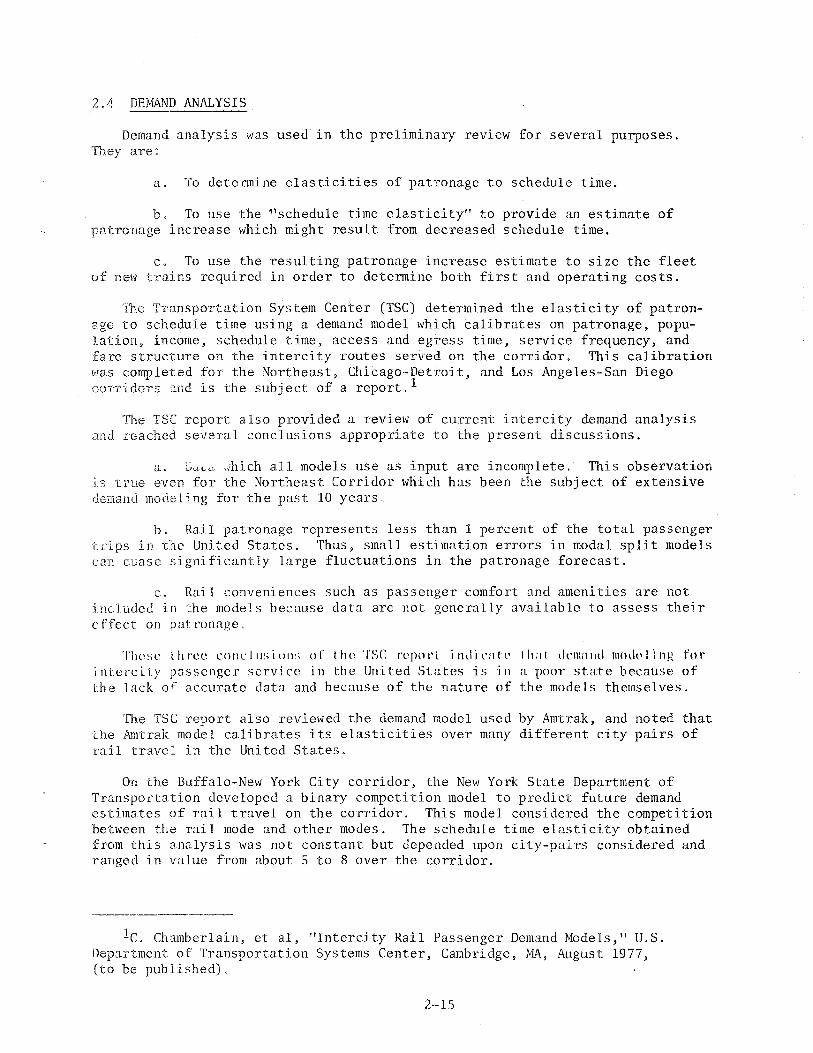
COMPARISON OF RIDE QUALITY LIMIT CRITERIA FOR RAIL VEHICLES •
LIST OF TABLES
Title
TRAIN REVIEW CRITERIA
CORRIDOR-RELATED DATA REQUIRED FOR TRAIN REVIEW , .
T~AIN-RELATED DATA REQUIRED FOR REVIEW, , , , ,
MINhlU,'~ REQUIREMENTS FOR RAIL VEHICLE FRONTAL STRENGTH, •
DATA REQUIREMENTS TO ASSESS ACCEPTABILITY OF CANDIDATE TRAINS BASED ON AAR STRUCTURAL STANDARDS, . , . , , .
v
2-10
2-14
2-24
2-2
2-11
2-12
2-31
2-32


1. INTRODUCTION
A number of new passenger train systems have been developed throughout the world and are now, or will be, available for possible utilization on United States railroads. Such trains include the Canadian LRC, the French TGV-PSE, the British APT and HST, the German ET403, the American SPV-2000; the Japanese Series 961; plus tilt body trains developed in .switzerland, Sweden, and Italy. While the complete trains are of interest, all employ components on subsystems (e.g., carbody banking systems, trucks, traction systems) having potential application in United States trains.
Early in 1977 the Federal Railroad Administration (FRA) initiated the Improved Passenger Equipment Evaluation Program (IPEEP) to conduct a systematic review of advanced trains and equipment now in operation or under development throughout the world, and to provide the results of the review to rail transportation system operators, planners, and developers.
1. 1 BACKGROUND
IPEEP is an outgrowth of the FRA Improved Passenger Train (IPT) program which began in 1973. The goal of the IPT program was to develop a prototype passenger tr::,~::-: +or application outside the Northeast Corridor (NEC) with provisions for converting to an all-electric traction system as opposed to a turbine cr diesel-electric system for application in the NEC. Early in the program it was determined that insufficient technical data existed to allow vigorous definition of IPT performance criteria or design specifications. Therefore, IPEEP focuses on providing the data needed for the subsequent development of a train performance specification; and this report describes the methodOlogy used to derive the technical data required to complete a review of existing foreign and domestic advanced trains.
1.2 TECHNICAL APPROACH
IPEEP has been structured as a 30-month program, focusing on review of foreign passenger trains and equipment against the requirements imposed by the United States railroad environment.
The trains reviewed in IPEEP are divided into two categories: electric trains having potential for NEC application, and fuel-burning trains having potential for application on routes outside the NEC.
1.3 TRAIN REVIEW
Initial work on IPEEP centered on train reviews. To assess the various trainsets in terms of the United States environment, the features and characteristics of the trains were matched against United States regulations and practices. The reviews were conducted by computer analysis to determine the expected performance of the trains in the corridors of interest. The NEC was modeled for the analysis of electric trains and these diesel-powered trains
1-1

were reviewed against four nonelectrified corridors: the Empire Corridor (Buffalo-New York City); a midwest corridor (Chicago-Detroit); a northwest corridor (Vancouver.,.Portland); and a southwest corridor (Los Angeles-San Diego).
Visits were made to the principal builders of each of the trains under r'evicw as well as to the respective railway companies that participated in the development of the train. The visits were made to obtain technical information and to become familiar with the operating environments for which the trains were developed. Technical data received from the train developers were used in a computerized mathematical model, called a train performance calculator (TPC), to determine trip time, energy consumption, and operating speeds for a given train operating in a given corridor. The participating trains were not reviewed against each other; instead, each was compared against equipment currently operating in the given corridor. In the NEe the baseline train for comparison was an upgraded Metroliner, and in the other corridors the baseline was an F40PH locomotive pulling Amcoaches, or the Amtrak Turboliner. The F40PH-Amfleet consist was the baseline on the Vancouver-Portland and Los Angeles-San Diego corridors. The Turboliner was the baseline train on the Buffalo-New York City and Chicago-Detroit corridors.
An overview of the trains reviewed and of the corridors used for performance simulation is contained in Volume 1 of the Train System Review Report.
The overall train review effort addressed the fo'llowing topics as criteria:
a. Patronage (expected patronage generated by the particular train).
b. Cost (capital and operating costs).
c. Passenger attraction (appeal and comfort) .
. d. Energy and environmental considerations (energy consumption and environmental pollution).
e. Safety.
f. Operational impact (operational flexibi Ii ty, on-time service capaci ty, and ease of maintenance) .
g. Degree of risk (development status and availability).
h. Special features (special features related to technical, operational, or passenger-related aspects) .
1-2
,/

2. METHODOLOGY
The methodology used to review passenger train potential capabilities on a given corridor was developed in several stages.
The first step was to determine the issues which could affect future rail passenger service and could have a significant influence on the equipment c.hoscn to provide this service. The issues were grouped into seven categories.
The second step was to divide each issue into well-defined criteria. The cri teria which are associated with each issue are listed in table 2-1 and are defined and described in paragraph 2.1. The criteria are both quantitative and quali tati ve in nature.
The third step was to describe a review process which could be carried out on each corridor/train combination and would flow into and from the background for the criteria. This would give an assessment of required corridor and tn.in data which were necessary for the review. The review procedure and required data are described in paragraph 2.2. This section also contains a detailed description of some of the submodels and computer programs used in the overall evaluation process.
Tn condu('t!~:, the train reviews it was not always possible to obtain sufficient data to allow all of the developed criteria to be considered for a given t rai 11.
2.1 CRITERIA
Schedule Time and Patronage
TIle NEC is being improved to provide high-speed train service capabilities between Washington and Boston for 1983 and subsequent years. The required objective is to provide 2-hour, 40-minute service between Washington and New York, and 3 .. hour, 40-minute service between New York and Boston.
A second, more stringent set of schedule times has been identified as desirable for the improved NEC; the times are Washington-New York in 2 hours 30 minutes, and New York-Boston in 3 hours. No such schedule time requirements have been established for other corridors.
The schedule time performance of each train is measured relative to the appropriate baseline train's performance on each of the respective corridors. Thus, the criterion for schedule time is relative performance.
Studies and statistical analysis of ridership in the United States and foreign countries have indicated that ridership bears a definite relationship to schedule time. For example, a decrease in train schedule time produces an increase in ridership.
2-1

TABLE 2-1. TRAIN REVIEW CRITERIA.
Issue Criterion
Schedule time and patronage That increasing patronage in a particular corridor be a result of decreased schedule time.
Cost
Passenger attraction
Energy conservation and environmental impact
Safety
Operational impact
Degree of risk
That new present ,value of life-cyc1e cost on a particular corridor for the particular piece of equipment be low.
That the equipment have a basic passenger appeal in both the amenities it affords the passenger as well as the comfort it provides.
That passenger equipment suit the corridor in both its ability to move people efficiently in terms of energy use and in its impact on the environmental quality of the corridor.
That the equipment provide safe movement of passengers through the corridor with respect to passenger and crew safety, vehicle safety in curves, and crashworthiness.
That the impact of the equipment on the corridor be satisfactory to rresent operations; namely, a high degree of flexibility, ability to achieve dependable service, and a high maintainability.
That in terms of development status, availability, and delivery time, the risk in procuring fleets of such equipment be minimized.
2-2

The patronage generated by any candidate train on nonelectrified corridors was calculated using a simple marginal change based on decreased schedule time of the candidate train over the present service:
liP t,T P Y T
where t,P/P represents the percent increase in patronage, t,T/T represents the decrease in schedule time, and y is the patronage/schedule time elasticity.
Performance with respect to patronage/schedule time will be indicated by:
a. Corridor patronage.
b, Percent patronage increase.
c. Percent schedule time decrease.
No attempt was made to include percent patronage increase as part of the review of Northeast Corridor trains because patronage increase estimates have been made by the Office of the Northeast Corridor Improvement Project.
Cost
A new train, or fleet of trains, must display a favorable cost-benefit ratio if it is to be a viable candidate for operation on the selected corridor.
The life-cycle costs should be estimated for each train within the 3.vailable data. These uata were not always available for all trains. don costs and import duties contribute to acquisition costs, but were into account because they cannot be estimated accurately.
limits of Modifica-not taken
The analysis period (or planning horizon) was taken as 25 years, which is the estimated useful life of major equipment, If there was strong evidence to the contrary, either a different useful life or a proper salvage value was adopted in selecting the analysis period.
Capital cost items that should be considered are:
a. Basic fleet for service.
b. Modifications to fleet to make it compatible with corridor operation.
c. Initial spare parts.
d. Maintenance support equipment and training.
e. Operational support equipment and training (initial).
Operating cost items that should be considered are:
a. CTew.
h. Maintenance (preventive, corrective).
2-3

c. Power or fuel.
d. Operation support.
Passenger Appeal
Appearance, decor, and amenltles can exert a significant influence on ridership, independent of variation in schedule speed. The ridership in the Los Angeles-San Diego corridor increased 50 percent without a schedule change when less attractive equipment was replaced with Amfleet cars in a highly publicized and advertised attempt to rejuvenate service.
The lack of firm conclusions on the degree to which amenities and comfort attract passengers necessitates a subjective assessment of passenger appeal. Comparisons were made with the baseline service on selected appeal items. Appeal items which have quantitative values are so evaluated. Those which have qualitative values were described.
Amtrak specifications for interior design, layout, and equipment would standardize many items affecting passenger appeal. These items, which include seat room, handicapped facilities, toilet facilities, baggage provisions, food service capability, and general appearance and decor, would be common to all subject trainsets.
The basic design, layout, and dimensions of each Lrainset would result in variations to the standard Amtrak format relating to:
a. Aisle width.
b. Window size.
c. Window layout with respect to seat spacing.
d. Illumination.
e. Door arrangement.
Qualitative aspects of each train such as the interior appeal due to the nature of the enclosed space (the Boeing 707 tunnel-effect appearance versus the Boeing 747 theater effect), the apparent ease or difficulty of movement between coaches, at doors, or in the aisles would also be considered in the train review.
It should be remembered, however, that modifications could be made to any train to improve passenger appeal. Therefore, seat room can be traded for aisle space, baggage provision and toilet facilities may be provided, and general appearance may be improved. These tradeoffs were considered in the evaluation.
Passenger Comfort
The general level of ride quality, audible noise, temperature control, and ventilation can determine whether a passenger will continue to utilize the service or revert to other modes of transportation.
2-4

\ \ , \
\ ~-- j
Passenger comfort was compared to present service on the corridor. Qualitative comparisons were made when quantitative measures were not available or data were insufficient. The following items are compared:
Item
Ride quaE ty
Interior noise level
Heating
Cooling
VeJltilation
~~ergy Consumption_
Index
Weighted vertical and lateral acceleration levels
A-weighted sound pressure level
Compared to baseline train
Compared to baseline train
Compared to baseline train
In view of the present efforts to conserve energy, energy consumption becomes an important criterion.
It shouJd be recognized that higher schedule speeds result in a greater amount of ene~g:r '::-onsumption if the train weight and aerodynamic drag are the SGme. However, with reduced weight and streamlining, a higher schedule speed may be achieved without increasing the energy consumption over that of present equipment. In this manner, decreased schedule time could be achieved without a concurre;1t increase in energy consumption. Energy consumption was estimated using the train performance program. Energy consumption is expressed in watthours or gallons per seat-mile, depending whether the train is electric or fuel burning.
Environmental Pollution
Two factors to be considered here are air pollution and external noise. These are items to which many communities and the Federal Government are becoming increasingly sensitive.
It is difficult to obtain actual numbers on exhaust pollution, although certainly one dividing line is electrified versus nonelectrified vehicles, and, for the latter, diesel versus gas turbine-powered. If insufficient data are available, air pollution comparisons will not be made. For the different types of powerplants, estimates may be based on their typical airflow and fuel consumption characteristics and their specific horsepower. Amount of various pollutants emitted per passenger-mile is the type of unit involved.
For nO_lse pollution, the exterior levels of noise, in terms of sound pressure level J which would be heard by a wayside observer would be used as the criterion. Air pollution comparisons wil1 not be made. As a matter of inforlIlat i on, the U.S. Environmental Protection Agency has accomplished a significant wnount of testing on railroad equipment noise emissions and is under a court mandate to issue, by early 1979, a new proposed regulation to limit noise emissions.
2-5

Operational Safety
The most serious situations of concern for passenger and crew safety are those of derailment, overturning, collision, and fire. The vehicles must be designed to withstand some level of the forces that may occur in these accidents. The following are the areas of consideration normally specified by Amtrak.
a. Although the vehicle may withstand the Association of American Railroads (AAR) buff load requirements, other elements of carbody construction should be studied. An example is the strength a carbody needs to withstand side impacts that may result from derailment.
b. Another carbody structural factor to be considered for trains transiting electrified territory must be the roof design relating to potential damage from pantographs and the catenary hardware. The roof area must have adequate strength to resist intrusion from above.
c. If at all possible, the vehicles should not uncouple following a derailment. The draft gear/coupler arrangement is extremely important. Strength and anticlimb devices should be primary considerations.
d. Window areas should be protected to reduce the potential for death or injury to passengers if the car turns on its side.
e. In case of fire, all precautions must be taken to insure passenger safety. particularly in the following areas:
(1) Fuel tank location, particularly on turbine-powered vehicles, is important.
(2) Firefighting equipment must be readily available aboard the vehicles to combat any local fire that might develop.
(3) At least four escape windows, two on each side, must be provided to afford easy egress.
(4) All interior !Ilaterials must be fire resistant: upholstery, seat padding, wall and ceiling lining, flooring, and carpeting. Some materials are fire resistant at room temperature but lose this characteristic once the fire is started and heat is generated.
f. The window glazing material must be adequate to resist missiles. At least one layer of nonbreakable material (polycarbonate) should be used at each window.
g. Handholds, steps, and other appurtenances should be designed to reduce the risk of injury to passengers boarding or leaving the trains. Sharp corners and objects should be avoided in the interior of the cars.
h. The intercar diaphragm openings should be carefully designed to eliminate any safety hazard that would be involved when the train is negotiating sharp curves and turnouts.
2-6

i. Consideration must be given to electrical equipment coolants that will be used in-the future. Polychlorinated biphenyls (askerel) are not being manufactured after 1977. This means that a nonflammable coolant such as silicone oil must be used to avoid a fire hazard.
Operational Flexibility
This criterion provides an assessment of the train's capability to respond to changing operating. conditions in the corridor. In the preliminary review, operational flexibility is qualitative and each of the following points is rated in comparison to the present service:
a. Change of consist size with varying demand.
b. Turnaround at intermediate terminals.
c. Turnaround time.
d. Ability to operate in the extremes of weather conditions experienced in the corridor.
e. Ability to mix with other Amtrak equipmenL
On-Time ~~~~:~e Capability
This criterion is a measure of the candidate train's ability to mInImIze delay under abnormal circumstances. In the preliminary review, this capability was qualitatively assessed using engineering judgment and plots developed to relate ability to recover from unscheduled slowdowns and diversions.
It includes:
a. Ability to make up time as a result of unexpected delays.
b. Ability to keep schedule time with partial loss of propulsion unit or component.
The review is principally based on amount of redundancy built into equipment and the acceleration as a function of speed of the train.
Ability to Maintain
Assessment of ability to maintain is subjective.
The following items are considered:
a. General layout of equipment for maintenance.
b. Utilization of modular components and assemblies,
c. Ease of coupling/uncoupling.
d. Overload and other malfunction protection.
e. Fault diagnosis.
2-7

f. Warning signals.
g. Ease of trucking/ de trucking operation
i. Preventive mai[\tt.'IElnl't~ l't.'quiremettts from point of vIew of lab~H'
and materials.
A qualitative value is placed on the ability to maintain as a result of reviewing a given train against items a through 1.
Development Status
The degree of risk incurred by purchasing and operating a fleet trains is partially determined by the status of train development. ing list indicates the status of trains according to development.
a. Design (paper only) .
b. Prototype (little testing).
c. Prototype (extensive testing).
d. Production (1-25 trains in service).
e. Production (more than 25 trains in service). j
of passenger The follow-
A second consideration in determining status was whether a train used many new technological components or mostly proven components. Extenuating circumstances which qualify ratings are described in each train review.
Availabi li ty and Deli very Time
This criterion is a measure of the ability to have a train available for operation in the corridor within the time constraints required by Amtrak.
Special Features
Special features, whether technical, operational, or passenger-related, were considered and described as a separate point in the review.
2. 2 REVIEW PROCESS
A block diagram of the overall review process is shown in figure 2-1. The corridor-related data necessary to carry through this process are listed in table 2-2, while the train data required are shown in table 2-3.
The corridor/train compatibility was determined by checking physical data and requirements, where available, including:
a. Clearance diagram.
b. Minimum radius curve.
2-8

c. Most severe crossover and track spacing.
d. Platform height (raised platform).
e. Distance to edge of platform.
.(:
.L. Track gage .
g. Electrified or nonelectrified.
h. Electrical characteristics if electrified.
i. Signaling system.
j . Corridor environmental conditions.
The train performance program provided the data for determining schedule time and energy consumption.
The patronage increase was determined from the incremental decrease in schedule time of the candidate train as compared with the baseline train. This was taken at 2.5-percent patronage increase per I-percent schedule time decrease over the baseline train.
With schedule speed and ridership determined, the fleet size and cost, together with spare requirements, were established.
Life--cycle cost estimates were established from these data after estimating operating cost and maintenance cost.
The other criteria are established as covered in paragraph 2.1 with the aid of computer programs and models described in subsequent paragraphs.
2.3 TRAIN PERFORMANCE PROGRAM
The portion of the model for the Train Performance Program utilized in this evaluation is shown in the simplified block diagram of figure 2-2. The Train Performance Model is presented in appendix A.
With reference to the block diagram of the train performance model, inputs are shown as a square block identified as either train or corridor. In the case of the speed restriction profile input, speed restrictions are functions of both the type of train and the corridor, thus the designation corridor/trai n data. The speed restrlction calculator tor curves is included as appendIX B; the specific route restrictions may be found in Volume 1 of the Train System Review Report.
The rounded blocks designate particular processing of both input data and output from intermediate processes.
Finally, summary outputs of schedule speed and fuel/power consumption on a station-to-station or an overall basis are shown as the end points of the processors.
2-9

N I I-'
o "----
I R
OU
TE
SE
RV
ICE
A
ND
PH
YS
ICA
L
CH
AR
AC
TE
RIS
TIC
S
(SIM
PL
IFIE
D)
TR
AIN
C
HA
RA
CT
ER
IST
ICS
(S
IMP
LIF
IED
)
SIM
PL
IFIE
D
DE
MA
ND
A
NA
LY
SIS
DE
TE
RM
INE
T
RA
I N
/RO
UT
E
CO
MP
AT
IBIL
ITY
INC
OM
PA
TIB
LE
T
RA
I N
/RO
UT
E
CO
MB
INA
TIO
NS
VIS
IT T
O
MA
NU
FA
CT
UR
ER
S,
OP
ER
AT
ING
RO
AD
S
MA
NU
AL
ES
TIM
AT
E
ES
TIM
AT
E
OF
EQ
UIP
ME
NT
R
IDE
RS
HIP
R
EQ
UI
RE
ME
NT
IM
PR
OV
EM
EN
T
CO
MP
ILA
TIO
N O
F
SIM
PL
IFIE
D T
RA
IN
LIF
E C
YC
LE
CO
ST
G
RO
SS
LIF
E
PE
RF
OR
MA
NC
E
RE
LA
TE
D I
ND
ICE
S
CY
CL
E C
OS
T
ES
TIM
AT
ES
SC
HE
D-
FO
R T
RA
IN/R
OU
TE
E
ST
IMA
TE
S
UL
E T
IME
C
OM
BIN
AT
ION
S
SIM
PL
IFIE
D
AN
AL
YS
IS
-O
F S
AF
ET
Y
SIM
PL
FIE
D A
NA
L-
YS
IS O
F P
AS
SE
NG
ER
~
CO
MF
OR
T A
ND
A
ME
NIT
IES
CO
MP
AT
IBL
E T
RA
IN/I
S
IMP
LIF
IED
AN
AL
-R
OU
TE
L
IST
ING
AN
D
YS
IS O
F E
NV
IRO
N-
SU
MM
AR
IES
,
ME
NT
AL
IM
PA
CT
(I
NT
EG
RA
TIO
N
I
OF
RE
SU
LT
S)
i
OP
ER
AT
ION
AL
-
AN
AL
YS
IS
DE
GR
EE
O
F R
ISK
FIG
UR
E 2
-1.
REV
IEW
PR
OC
ESS.

TABLE 2-2. CORRIDOR-RELATED DATA REQUIRED FOR TRAIN REVIEW.
Service Data
Cities served Distance between stations Amtrak equipment Amtrak schedules (time and frequency) Fa:re structure Operating railroads, terminals, maintenance facilities Station access times (where applicable) Present rail travel patterns and trends Degree of industrialization and freight traffic
Right-of-way
Clearance diagram Track curvature lraciz g:rades
Physical Data
Present speed restrictions (civil versus train dependent)
Stations
Platforms Description of station condition Station access
Signals and communications
Description of system noting any peculiar restricting problems (such as lack of cab signals = 79 mi/h top speed)
Block lengths Track circuit characteristics
Special restrictions
Future Plans for Corridor Rail Improvement
Description of characteristics of corridor which might be relevant to particular kinds of trains (such as curves, turnaround requirements,
etc.)
2-11

N I ......
N
a,
b,
c,
TABL
E 2-
3.
TRA
IN-R
ELA
TED
DA
TA
REQ
UIR
ED
FOR
REVI
EW
Dra
win
g ty
pe
info
rmat
ion
req
uir
ed
(1)
Cle
aran
ce d
iag
ram
(2
) E
quip
men
t lo
cati
on
sc
hem
atic
(3
) T
rain
co
nfi
gu
rati
on
s (v
eh
icle
mak
eups
) (a
) T
rain
le
ng
th
(b)
Max
imum
nu
mbe
r o
f p
asse
ng
ers
(4)
Desc
rip
tio
n a
nd
typ
es
of
cars
Bas
ic
veh
icle
dim
ensi
on
s
(1)
Len
gth
o
ver
co
up
lers
(2
) L
eng
th
ov
er b
uff
ers
(3
) P
anto
gra
ph
lo
ckdo
wn
heig
ht
(ele
ctr
ic)
(4)
Max
imum
p
anto
gra
ph
ru
nn
ing
h
eig
ht
(ele
ctr
ic)
(5)
Car
body
h
eig
ht
(6)
Dis
tan
ce b
etw
een
tr
uck
cen
ters
(7
) C
arbo
dy
wid
th
(max
imum
at/
heig
ht)
(8
) H
eig
ht
of
carb
od
y
abo
ve
rail
(m
axim
um)
(9)
Av
erag
e ca
rbo
dy
w
idth
(l
0)
Fro
nta
l are
a
(lea
d
cars
o
nly
) (1
1)
Ave
rage
ca
rbo
dy
le
ng
th
(12
) T
ruck
wh
eel
bas
e (1
3)
Ax
le
cen
ters
(l
4)
Min
imum
cu
rva
tu r
e
rad
iu
s (1
5)
Cen
ter
of
gra
vit
y h
eig
ht
(16)
M
axim
um
late
ral
off
set
of
cen
ter
of
gra
vit
y
(17
) C
ou
ple
r h
eig
ht
(18
) P
latf
orm
heig
ht
req
uir
ed
Sta
tic
and
dyna
mic
wei
gh
ts
(1)
Wei
ght
in w
ork
ing
o
rder
(2)
Max
imum
w
eig
ht
wit
h
full
p
asse
ng
er
load
(3
) W
eigh
t p
er
axle
(4
) W
eigh
t o
n d
riv
ing
ax
les
(5)
Uns
prun
g w
eig
ht
(6)
Seats
/car
(2)
(3)
(4)
(5)
(6)
(7)
(8)
(9)
(10
)
Pro
pu
lsio
n (e
lectr
ic v
ers
ion
) (a
) L
ine
vo
ltag
e
(no
min
al,
max
imum
, ~inimum)
(b)
Lin
e fr
equ
ency
(n
om
inal
, m
axi"
,,,,,,
. m
inim
um)
(c)
Pow
er
con
sum
pti
on
-lin
e kw
vs
tra
ctiv
e eff
ort
an
d sp
eed
(d)
Desc
rip
tio
n o
f w
heel
sli
p
co
ntr
ol
(e)
Dy
nam
ic/r
egen
erat
ive
Au
xil
liary
po
wer
re
qu
irem
ents
(k
W
and
.....
A)
Tru
cks
(a)
Typ
e an
d o
utl
ine d
raw
ing
(b
) p
r im
a ry
su
spen
s io
n
1 S
pr
ing
s '2
Dam
ping
(c
) S
eco
nd
ary
su
spen
sio
n
1 S
pri
ng
s '2
Dam
ping
(d
) A
xle
an
d jo
urn
al
size
(e)
Whe
el
dia
met
er
(max
imum
, m
inim
,,::.)
B
rak
ing
sy
stem
(a
) D
esc
rip
tio
n a
nd
sch
emat
ic
(b)
Fri
cti
on
/dy
nam
ic b
rak
e b
len
din
g
sch
edu
le
(c)
Desc
rip
tio
n o
f w
heel
sl
ide co
ntD
l C
oup
lers
(a
) T
ype
and
desc
rip
tio
n
(b)
Bu
ff
and
dra
ft
stre
ng
th
Com
mu
nic
a ti
on>
; (a
) T
rain
ra
dio
desc
rip
tio
n
(b)
Cab
si
gn
als
d
esc
rip
tio
n
(e)
Pu
bli
c
add
ress
d
esc
rip
tio
n
Tra
in co
ntr
ol
and
pro
tecti
on
(a
) D
esc
rip
tio
n o
f sy
stem
(b
) S
peed
co
ntr
ol
Pan
tog
rap
h (e
lectr
ic v
ersi
on
) (a
) T
ype
and
desc
rip
tio
n
(b)
Max
imum
sp
eed
P
asse
ng
er a
men
itie
s an
d co
mfo
rt
(a)
Rid
e
qu
aH
ty
ch
ara
cte
r is
tics
1 A
ccele
rati
on
and
je
rk
'2 L
ate
ral
and
vert
ical
forc
es

N I ......
V-l
TABL
E 2-
30
TRA
IN-R
ELA
TED
DA
TA
REQ
UIR
ED
FOR
REV
IEW
(c
on
tin
ued
)
d.
e.
S t re
ng
t hs
(1)
Co
mp
ress
ive
load
s (a
) A
t cen
terl
ine d
raft
(b
) T
wel
ve
inch
es
abov
e cen
terl
ine d
raft
(2
) B
uf f
load
(3
) C
oll
isio
n
po
st sh
ear
stre
ng
th at
bo
tto
m
con
nec
tio
n
(4)
Ant
icli
mb
er
cap
acit
y
(5)
Str
uctu
ral
arra
ng
emen
t (t
o
chec
k d
esi
gn
ag
ain
st a
pp
licab
le
rule
s an
d st
an
dard
s)
(6)
Tru
ck
to
carb
od
y
atta
chm
ent
(a)
Vert
ical
(b)
Sh
ear
(7)
Jack
ing
p
rov
isio
ns
Per
form
ance
ch
ara
cte
rist
ics
(1)
Max
imum
se
rvic
e
spee
d
(2)
Max
imum
tr
acti
ve eff
ort
(3
) C
on
tin
uo
us
tract
ive
eff
ort
(l
bs
at
mi/
h)
(4)
One
h
ou
r ra
tin
g
(HP
@ m
i/h
) (5
) C
on
tin
uo
us
rati
ng
(H
P @
mi/
h)
(6)
Ad
hes
ion
li
mit
(e
nv
elo
pe
of
tracti
ve eff
ort
v
s sp
eed
) (7
) T
racti
ve eff
ort
v
s sp
eed
(p
rop
uls
ion
) (8
) T
racti
ve eff
ort
v
s sp
eed
(s
erv
ice
bra
ke)
(9
) T
ra<
:tiv
e eff
ort
v
s sp
eed
(e
mer
gen
cy
bra
ke)
(1
0)
Tra
in
resi
stan
ce (i
f m
easu
red
) .
Eo
Su
bsy
stem
ch
ara
cte
rist
ics
(1)
Pro
pu
lsio
n
(no
nele
ctr
ic
vers
ion
) (a
) D
ese
rip
t io
n
and
sche
ma ti
c
(b)
Po
wer
/wei
gh
t ra
tio
(c
) A
nti
po
llu
tio
n
syst
em
-desc
rip
tio
n
and
sch
emat
ic
(d)
Cu
rves
o
f fu
el
con
sum
pti
on
vs
tr
acti
ve eff
ort
an
d sp
eed
(e)
Desc
rip
tio
n
of whee~
sli
p
co
ntr
ol
(b)
(c)
(d)
Fu
rnis
hin
gs
and
facil
itie
s
1 S
eati
ng
2"
Bag
gage
3
Win
dow
s la
yo
ut
a D
imen
s io
ns
b N
umbe
r e
Mate
rial
d S
tren
gth
4
Foo
d se
rvic
es
cap
ab
ilit
y
5 T
oil
et
facil
itie
s
a N
umbe
r b
Lo
cati
on
c
Sy
stem
desc
rip
tio
n
6 H
and
icap
ped
fa
cil
itie
s
7" L
igh
tin
g
En
vir
on
men
tal
co
ntr
ol
1 H
eati
ng
a
Typ
e an
d d
esc
rip
tio
n
b P
ower
re
qu
irem
en
ts
2 A
ir-c
on
d iti
on
ing
a
Typ
e an
d d
esc
rip
tio
n
b P
ower
re
qu
irem
ents
3
Insu
lati
on
an
d w
eath
er se
als
-
a C
abin
b
Doo
rs
Inte
rnal
no
ise le
vels
1
Sp
ecif
icati
on
s fo
r p
asse
ng
er
and
crew
co
mp
artm
ents
2"
N
ois
e in
sula
tio
n
tech
niq
ues
(e)
Doo
rs
1 T
ype
and
locati
on
2"
D
esc
rip
tio
n o
f co
ntr
ol
syst
em
3 C
losi
ng
p
ress
ure
s 4
Safe
ty
featu
res
g.
En
vir
on
men
tal
imp
act
(1)
Po
llu
tio
n le
vels
(2
) E
xte
rnal
no
ise d
ata
(a
) S
ho
rt
dis
tan
ces
(b)
Lon
g d
iata
nces

N I >-'
~
TR
AIN
D
AT
A
CO
NS
IST
CH
A R
AC
TE
RIS
TI
CS
TR
AIN
D
AT
A
VE
HIC
LE
D
IME
NS
ION
AL
CH
AR
AC
TE
RIS
TIC
S
(FO
R E
AC
H V
EH
ICL
E
IN T
RA
IN)
TR
AIN
D
AT
A
PO
WE
RE
D V
EH
ICL
E
PR
OP
U L
SIO
N A
ND
CO
NT
RO
L
CH
AR
AC
TE
RIS
TIC
S
TR
AIN
D
AT
A
VE
HIC
LE
BR
AK
ING
AN
D C
ON
TR
OL
CH
AR
AC
TE
RIS
TIC
S
T"'
::"'
:'\.
""::
5 5
T A
'\,C
E
AS
~~~~CT!O"'"
01=
5"::
:E 0
TR
AC
TIV
E A
ND
3R
AK
If\,
G E
FF
OR
T
AS
F
li ...
. CT
IQN
O
F
SP
EE
D A~D C
ON
TR
OL
CH
AR
AC
TE
RIS
TIC
CO
RR
IDO
R D
AT
A
GR
AD
E A
ND
..'lo
LIG
NM
EN
T
PR
Ofi
LE
AC
CE
LE
RA
TIN
G
AN
D B
RA
KIN
G F
OR
TR
AIN
,.
\5 F
UN
CT
ION
OF
SP
EE
D A
ND
CO
NT
RO
L
1 T
RA
IN D
AT
A
PO
WE
RE
D V
EH
ICL
ES
PO
WE
R/F
UE
L
CO
NS
UM
PT
ION
CH
AR
AC
TE
RIS
TIC
S
CO
RR
IDO
R/T
RA
IN D
AT
A
SP
EE
D
RE
ST
RIC
TIO
N
PR
OF
ILE
1
SP
EE
D R
ES
TR
ICT
ION
TO
CO
MM
AN
D
CO
NV
ER
TE
R
SP
EE
D,
TIM
E,
TR
AC
TIV
E A
ND
BR
AK
ING
EF
FO
RT
AS
FU
NC
TIO
N
OF
TRAI~
PO
SIT
ION
IN
CO
RR
IDO
R
FU
EL
/PO
WE
R
CO
NS
UM
PT
ION
A
S
FU
NC
TIO
N O
F P
OS
ITIO
N
TIM
E IN
CO
RR
!DO
R
F'IG
UR
E 2
-2.
SIM
PLIF
IED
BL
OCK
D
IAG
RAM
O
F TR
AIN
PE
RFO
RMA
NCE
M
OD
EL.
--.
CO
RR
IDO
R D
AT
A
ST
AT
!ON
AN
D
DW
EL
L T
IME
PR
OF
ILE
SU
MM
AR
Y O
UT
PU
T
SC
HE
DU
LE
SP
EE
D A
ND
TIM
E
SU
MM
AR
Y O
UT
PU
T
FU
EL
/EN
ER
GY
CONSU~PTION
FO
R T
R!P
2.4 DEMAND ANALYSIS
Demand analysis was used in the preliminary review for several purposes. 1118Y are:
a. To determine elasticities of patronage to schedule time.
b. To use the 11schedule time elasticity" to provide an estimate of patronage increase which might result from decreased schedule time.
c. To use the resulting patronage increase estimate to size the fleet of new trains required in order to determine both first and operating costs.
The Transportation System Center CTSC) determined the elasticity of patronage to schedule time using a demand model which calibrates on patronage, population, income, schedule time, access and egress time, service frequency, and fare structure on the intercity routes served on the corridor. This calibration \lIaS completed for the Northeast, Chicago-Detroit, and Los Angeles-San Diego conidoys and is the subject of a report. 1
The TSC report also provided a review of current intercity demand analysis and reached several conclusions appropriate to the present discussions.
a. [".<.L.e' .,chich all models use as input are incomplete. This observation is true even for the Northeast Corridor which has been the subject of extensive demand modeling for the past 10 years,
b. Rail patronage represents less than 1 percent of the total passenger trips in the United States. Thus, small estimation errors in modal split models caB cuase significantly large fluctuations in the patronage forecast.
c. Rail conveniences such as passenger comfort and amenltles are not included in the models because data are not generally available to assess their effect on patronage.
These thr'ee cOllclusioll:; of the 'l'SC rCJlOt'l intiic:lte thill dl'llIll1ld l11Cllh'lillg 1'01' interc i ty passenger service in the United States is in a poor state because of the lack of accurate data and because of the nature of the models themselves.
'The TSC report also reviewed the demand model used by Amtrak, and noted that the Amtrak model calibrates its elasticities over many different city pairs of rail trave 1 in the Uni ted States.
On the Buffalo-New York City corridor, the New York State Department of Transportation developed a binary competition model to predict future demand estimates of rail travel on the corridor. This model considered the competition between the rail mode and other modes. The schedule time elasticity obtained from this analysis was not constant but depended upon city-pairs considered and ranged in 'value from about 5 to 8 over the corridor.
lC. Chamberlain, et aI, "Intercity Rail Passenger Demand Models," U.S. Department of Transportation Systems Center, Cambridge, MA, August 1977, (to be published).
2-15

As a result of the review of the state of these models as well as the conclusions of the TSC report, the following conclusions were appropriate:
a. The only patronage increase that can be expected should be that due to the s~hedule time of the train to be evaluated. Access and egress time, departure frequencies, and fare structures, although affecting patronage, are determined primarily by operational conditions and constraints, and as such, would not vary according to the train system considered for evaluation.
b. Because passenger amenities and comfort conditions of the train affect patronage in ways which are not understood, these evaluation criteria nre considered separately from patronage, and primarily as judgmental factors.
c. Percentage patronage increase should be taken as two to three times the percent decrease in schedule time based on the TSC report. This relation should be independent of corridor or city-pair considered.
As a result of these arguments, patronage increase is equated to schedule time decrease by the relation
t.P = t.T P 2.5 T
were 6T/T is the percent change in schedule time of the train to be evaluated over the present service, and 6P/P is the percent increase in patronage expected over the present service. The elasticity, 2.5, is corridor independent for the purpose of this analysis.
It should be recognized that patronage increase is related to schedule time decrease; thus, for purposes of the evaluation, schedule time is the important criterion. The only use made of patronage increase. will be in fleet determination for cost purposes.
2.5 TRAIN SAFETY IN CURVES
Introduction
The objective of the steady-state curving simulation was to establish the equilibrium configuration of the two-axle truck negotiating a constant-radius curve at constant speed. The equilibrium configuration can be determined by simultaneously solving the equations of motion when the damping and transient inertial forces are zero. The reduced equations of motion are linear In the dependent variables (degrees of freedom), However, many of the coefficents of the dependent variables are not only nonlinear, but also a function of the magnitude of the dependent variables. To simultaneously solve the complete set of nonlinear equations is a difficult mathematical task. Perhaps more difficult is to quantitatively establish the value of the nonlinear coefficients (e.g., the primary lateral stiffness as a function of the relative displacement between the wheelset and truck frame). Even such coefficients as linear viscous damping coefficients and moments of inertia are often not available, and must be obtained from engineering estimates.
2-16

In spite of the lack of detailed vehide characteristics, there are several nonlinear phenomena which are known and C3.n be approximated in the solution. Therefore, the solution technique used in this simulation was a multistep iteration of the quasi-linear equations of motion.
Assumptions
lnc basic set of equations of motion was defined for seven degrees of freedom of a rigid-frame, two-axle passenger truck (appendix C). The degrees of freedom were lateral and yaw for each of two axles, and lateral, yaw, and roll for the rigid truck frame. In addition to internal forces acting through the suspension parameters, centrifugal and gravitational forces were assumed to act at the center of gravity of each axle and of the truck frame. Centrifugal, gravitational, aerodynamic, and buff loads acting on the carbody were transferred to the truck frame as roll and yaw moments and lateral forces. The resulting solution of the equations, therefore, included not only the natural curving forces of either a leading or trailing truck, but also the effect of half of the external forces acting on the carbody.
';1,6 nonlineari ties included in the simulation were lateral secondary suspensicE stops, creep coefficients as a function of wheel load, maximum creep fon:e as Q funct ion of adhesion coefficient, and flange force as a function of lateral whf;elset displacement. Lateral carbody displacement relative to the truck frame was calculated and limited to the maximum lateral secondary suspensiun displacement. Inside and outside vertical wheel loads were established by calculating the overturning moment on the truck frame due to centrifugal, gravitational, aerodynamic, and buff loads. The total creep plus gravitational force per axle was limited to the adhesion coefficient times the axle load. This was accomplished by an iteration procedure on the creep coefficients. The flange forces were determined by assuming, one at a time, all possible configurations of flanging conditions and checking the solutions as to their physical possibili ties.
lni tial creep coefficients included both the longitudinal and latera1 components, and were determined as a function of wheel radius and whee1 load as established by Kalker. 2 Half of Kalker's creep coefficients were used because tests have shown that the foreign matter that usually accumulates on rail reduces the theoretical value of Kalker's creep coefficient by approximately half.
For the tilt-body passenger vehicles which were simulated, two additional input variables (roll center location and active roll angle) were used in the calculation of the vertical wheel loads. As a first approximation, the active roll angle (degrees) was set equal to the vehicle unbalance in inches ea positive roll angle implies the top of the carbody is rotated inward toward the center of the curve). Al though some active tilt systems do have the capability of keeping the carbody center of gravity centered over the track, this simulation did not include that effect. If the vehicle had a self-centering capability, the simulation would predict a slight1y 10wer vertical wheel load on the inside wheels, a conservative prediction.
2J.J. Kalker, "On the Rolling Contact of Two Elastic Bodies in the Presence of Dry Friction,if Doctoral Dissertation, Technische Hogeschool, Delft, Netherlands, 1967.
2-17

Simulation Inputs and Outputs
Since the solution is a steady-state condition, damping and inertia terms are not required. However, component weights are necessary to determine centrifugal loads, vertical wheel loads, creep coeficients, and gravitational stiffnes~. All suspension stiffness elements between the wheelsets and truck frame, antI hetween the truck frame and carbody, along with their locations, are needed. l~e overall dimensions of the components and their center of gravity locations arc also necessary inputs.
The basic outputs of the simulation are the equilibrium displacements of the seven degrees of freedom of the truck. Knowing these variables, all the forces acting internally or externally to the system can be calculated. In particular, the vertical and lateral wheel/rail forces acting at each of the four wheels were determined, and combined to yield those values necessary to establish the relative safety of the vehicle.
Safety Criteria for Curving
Pour separate criteria were considered to determine the safety of the raH vehicle3 :
a. Vehicle overturning stability.
b. Wheel-climb derailment capability.
c. Rail rollover capability.
d. Lateral track shift capability.
Pirst, the load ratio was calculated for each of the four wheels by dividing the steady-state vertical wheel load in the curve by the nominal tangent track wheel load. These four parameters and especially those of the two inside wheels are a measure of vehicle overturning stability. The limiting value is 0.4 when a 15 psf (77 mi/h) wind load is acting on the side of the carbody. In general, load ratio is not a function of c~rvature, but only of vehicle unbalance.
The second safety factor measures wheel-climb derailment capability. A maximum value of 1.0 for the ratio of lateral to vertical force (L/V) on a single wheel for time durations of the lateral force pulse greater than 50 ms is a dynamic criterion. However, a quasi-static value, as determined by this L/V, should be substantially less than 1.0 to provide safety during transient events. Although, for a given curve, any of the four wheels may have the highest L/V, the outside front wheel develops the highest L/V's for the high Cllr
vature, high unbalance curves. When the outside front wheel L/V is not the highest of the four wheels, all four wheels have relatively low L/V's.
3p. E. Dean and D. R. Ahlbeck, "Criteria for the Qualification of Rail Vehicles for High-Speed Curving," Working Paper Por IPEEP, Battelle's Columbus Laboratories, Colt~bus, Ohio, September, 1977, (unpublished).
2-18

Truck L/V is defined as the ratio of the total lateral force to the total vertical force exerted by one truck on one rail. Its value measures rail rollover or gage widening derailment probability. The maximum safe value is 0.55 +
2300/Pw' where Pw = the static load on a single wheel.
The last safety criterion is the maximum lateral force on a single wheel, Fc. which ascertains that no permanent lateral deformation of the track occurs. Its maximum value depends on track condition and axle load:
Fc A(0.4P + 2700) pounds for new or newly worked wood tie track
where Fc A(0.7P + 6600) pounds for compacted wood tie track,
A 1 for bolted rail A 0.96 - 0.0200 for CWR, 0 = curvature, degrees P axle load, pounds
Note: CWR (continuous welded rail) has a lower value than bolted rail.
2.6 OPERATIONAL FLEXIBILITY ANALYSIS
The operational flexibility is dependent upon the feasibility of changing train consist and ease of turnaround. These factors, in turn, depend upon the number of counlinrrs, the configuration of the train consist, and track arrangements for turning equjplJlent.
Turnaround
There are three basic turnaround situations dictated by three possible equipment configurations. All three situations occur with the equipment involved in this review. The configurations are as follows, arranged in order of increasing turnaround time.
a. Double-ended trainset. This requires no turnaround other than replenishing supplies and making routine terminal (brake) tests. Metroliners and other multiple-unit cars fit this category, as do the present Turboliners.
b. Train with double-ended locomotive. Turnaround requires uncoupling the locomotive and moving it to the other end of the train, in addition to the replenishing and testing functions noted above. Amcoaches hauled by back-toback F40Pl-l diesels are examples of this category.
c. Train with single-ended locomotive. Turnaround is longest for this type of equipment, since the locomotive must be uncoupled and taken to an appropriate turning facility, such as a "Y", in addition to all other terminal servicing noted above. A train of Amcoaches hauled by F40PH diesels with cab oriented in the same direction, is an example of this category_
In tllC two cascs cited last, the time required to move the locomotive is largely a function of terminal layout, especially where single-ended locomotives must be turned around. Depending on the availability of a reverse loop, the entire train may be turned in less time than it would take to uncouple the locomotive, turn it separately, and recouple.
2-19

Coupling and Uncoupling Operations
A coupling or an uncoupling operation may depend upon many situations, all of which will effect time loss. The following were considered in the evaluation:
a. Articulation and married pairs. Improbable that two articulated cars could be uncoupled and coupled during normal operation.
b. Mechanical coupling/uncoupling. Includes engagement/disengagement of the couplers, adjustments or diaphragms, or other peripherals which are mechanical in nature.
c. Electrical coupling/uncoupling. Includes low voltage, low current train line wires, cables for auxiliary and/or traction power circuits, and high voltage (catenary value) circuits which may be coupled between two cars.
d. Pneumatic or hydraulic coupling/uncoupling. Would generally include air-brake lines, steam heating lines, or hydraulic fluid lines, if applicable.
The degree of automation of the tric couplers was also recognized. operation were also considered.
2.7 RIDE QUALITY ANALYSIS
Introduction
coupling/uncoupling procedure such as elecRequirements for switcher locomotives in the
One of the objectives of the train review phase of the program was to develop standard methods and techniques for the evaluation of passenger train equipment. An important area in this technical review is passenger ride quality. Several criteria are available to quantify ride comfort. Basically, these criteria involve weightings of the vertical and lateral carbody accelerations measured or calculated (using computer simulations) over an elapsed time period during which the vehicle is running over some section of traCK. The acceleration time-histories are functions of track geometry and condition as well as vehicle speeds and vehicle/suspension design. Accordingly, care must be taken when comparing any such measured or calculated ride quality data to insure that differences in track geometry are absent or compensated for.
The ride quality criteria in use throughout the world also differ considerably. These differences are due to the following factors:
a. Different weighting factors are used, based on frequency, human sensitivity, and direction of motion.
b. Accelerations are measured as peak values, or as root-mean-square (rms) values.
c. Accelerations are combined to give an overall ride index number which eliminates all frequency information, or are plotted as a function of frequency to give a curve of acceleration level versus frequency.
d. Frequency is expressed in different ways; for example, octave bands, third-octave bands, or finer frequency bands.
2-20

Due to the factors mentioned above, it is difficult to obtain meaningful comparisons of vehicle ride from published data, because it is usually stated in terms of one or two values of one of the ride indices, with little or no information pertaining to the track or conditions under which this data was obtained.
When sufficient data on vehicle characteristics are :Ivai lable, comparative ride quality characteristics of different vehicles can be obtained by means of computer simulation of vehicle and track. This eliminates the track as an unknown value, since the track geometry is one of the inputs, and is specified (and varied, if desired). This was the approach used in this train review project. To quantify the ride quality of the various vehicles, a 14-degree-offreedom frequency domain computer simulation was developed and the computed results were expressed in terms of the appropriate ride criteria.
Vehicle Model
The model used to establish ride quality was a linear, lumped-parameter simulation of a rail vehicle. Since ride quality is generally a function of the random irregularities of the track plus discrete spectral peaks (caused by the 39 ft. rail length), it was necessary to study the vehicle's response in the frequency domain. The input consisted of power spectral densities (PSD) of rail alignment, surface, and cross level irregularities; the output was a PSD of the vertical and lal.eLal acceleration of the carbody. The output accelerations were weighted according to comfort criterion, and a single ride index was calculated to relate the car-body accelerations to a subjective ride quality.
Linear spring, damper, and mass values were used, and the computer program used was the TRKVPSD MOD IB program (appendix D). The vehicle characteristics were obtained from a number of sources, including manufacturer's data, test results, and engineering estimates. Some parameters, particularly the damping values, are at best a small-motion approximation of the basically nonlinear response of friction or hydraulic elements. Mass moments of inertia are generally engineering best estimates, although some of the values have been confirmed by natural frequencies measured in tests.
Comfort Criteria
Perhaps the two most widely accepted criteria for establishing ride quality or rail vehicles are the tlWz" ride index developed by the German Federal Railway,4 and the International Standard ISO 2631 "Guide for the Evaluation of Human Exposure to Whole-Body Vibration."S Both of these criteria have been the subject of diverse criticism. The "Wz
tl rating has in the past been favored by the British Rail (BR), the Swedish State Railway (SJ) , the German Federal Railway (DB) and others; while the ISO Standard has been favored by the French National Railway (SNCH) and has gained support in recent years from other rail-
lf Dr . E. Sperling, "Position of Ride Quality Analysis, Measurement and
Computation," 1968, Eisenbahntechnik, translation by University of New Hampshire, Center for Industrial and Institutional Development.
5International Standards Organization "Guide for the Evaluation of Human Exposure to Whole-Body Vibrations," ISO/DIS 2631, 1974.
2-21

way administrations. A state-of-the-art discussion of ride comfort has been compiled from the 1975 Ride Quality Symposium sponsored by the National Aeronautics and Space Administration (NASA) and the U.S. Department of Transportation. 6
Vibration limits used by the Japanese ~ational Railway (JNR)7 are based on the older limits established by Janeway.8 9 Basic differences in the limits endorsed by these three criteria are illustrated in figure 3 for both vertical and lateral directions of motion. In this figure, the limits for the ISO 2.5-hour reduced comfort limit, the "almost-good" rating (W z = 2.5), and the JNR "Category 1" (very good) ride quality are compared. Interpretation of these limits poses some difficulty: the ISO reduced comfort time is based on all third-octave rms acceleration values being equal to or less than the limit, while the Wz limit implies that only one, predominant acceleration component could reach the plotted limit (if more than one component were at the limit, the Wz rating number would be higher). Janeway's limits, on which the JNR comfort limits are based, were established for single-frequency sinusoidal accelerations, and the superposition of broad-band frequency components was not addressed.
While the ISO reduced-comfort limits are presented for vertical and horizontal (lateral or longitudinal) axes, the JNR specification calls for a separate limit for the longitudinal, with a minimum of 0.025 g from 4 to 15 Hz, rising to 0.10 g at 60 Hz. While there is a tendency to ignore the longitudinal axis, this can be the source of some very annoying low-frequency oscillations. Support provided by the passenger seat back undoubtedly has a significant effect on ride comfort in the lateral versus the longitudinal axis.
The Wz method of rating the ride quality of a rail vehicle was developed in the early 1940's by Helberg a~d Sperling in Germany to relate measured accelerations with a single ride quality. The previously cited article by Sperling described how the method is employed by the Deutsches Bundesbahn using modern instrumentation and recording techniques. An acceleration signal is integrated over some time period (typically 1 to 2 minutes), and individual third-octave rms acceleration values are weighted and summed to calculate an overall Wz factor:
Wz where:
B· 1 A· 1
=
7.89 [ZCBiAi)2JO.15
weighting function at ith third-octave center frequency, carbody acceleTation in ith third-octave band, g rms.
61975 Ride Quality Symposium, NASA Langley Research Center, Report No. NASA TM X-3295, DOT-TSC-OST-75-40, November 1975.
7T. Matsudiara, "Dynamics of High Speed Rolling Stock," JNR RTRI Quarterly Report, Special Issue, Aug. 1964, pp. 24.
8R. N. Janeway, "Human Vibration Tolerance Criteria and Applications to Ride Evaluation," SAE Paper No. 750166, February 24-28, 1975.
gR. N. Janeway, "Analysis Qf Proposed Criteria for Human Response to Vibration," 1975 Ride Quality Symposium, NASA Langley Research Center, Report No. NASA-Tl'i X-3295, DOT-TSC-OST-75-40, Paper No. N76-16776, pp. 531-563.
2-22

The weighting functions are the inverse of the curve shapes shown in figure 2-3. Note thnt the lnteral weighting function is identical in shape with the vertical, with the most sensitive frequency at 5 Hz. It is the sensitivity in the lateral direction that is the most important difference between the Wz and ISO weightings. The resulting Wz index is then compared with the following subjective ranking:
1 - very good 2 good 3 satisfactory (an upper limit for passenger cars) 4 tolerable (more typical of freight cars) 5 dangerous in service
I\s a comparative example, the Australian New South Wales (NSW) railway designers consider the following worst-riding ranges as satisfactorylO:
Main line equipment Suburban equipment Locomotives
2.5 to 2.75 3.0 to 3.25 3.5 to 3.75
The ISO Standard 2631 for evaluation of human response to vibration was developed over a 10-year period, starting in 1964 with the work of Technical Committee 108. 11 In the vertical axis, the ISO weighting reflects a frequency range of maximnm ~ensitivity from 4 to 8 Hz; while in the horizontal (transverse) axis the greatest sensi ti vi ty is in the 1- to 2-Hz range, reflecting the investigations of Pradko12 and Lee13 using the absorbed-power concept. These weighting functions are given in figure 2-3 and are used to calculate an overall weighted acceleration value:
where
Ci = ISO weighting factor at the ith third-octave band center frequency
A. measured acceleration in the i th third-octave band, g rms 1
The resulting weighted acceleration value is then compared with the acceptable acceleration level (at the most sensitive frequency) for the "reduced comfort boundary," which is "related to the difficulties of carrying out such operations as eating, reading, and writing. For the "S-hour reduced comfort boundary," the acceptable levels are:
IOH. E. Coxon and L. D. McNaughton, "Bogie Design for Australian Conditions," The Railway Engineering Journal, March 1973, pp. 16-31.
IIG. R. Allen, Ride Quality and International Standard ISO 2631 ("Guide for the Evaluation of Human Exposure to Whole-Body Vibration") .
12F. Pradko and R. A. Lee, "Vibration Comfort Criteria," SAE Paper 660139, 1966.
13R. A. Lee and F. Pradko, "Analytical Analysis of Human Vibration," SAE Paper 680091, 1968.
2-23
(/) :2: a:
(:J
o. K
/
V
" /
V
/
......
" //
/ //
..... ~
" l'L
--/
"-/
/ ,
!
~-
-----
-i
, ~ --
-//
, I
JNR
"C
AT
EG
OR
Y I
" L
IMIT
---
VE
RT
ICA
L A
CC
EL
ER
AT
ION
0.0
5
0.0
3
0.0
2
_..J
ISO
2.5
HO
UR
RID
E C
OM
FO
RT
LIM
IT
l.LJ >
l.LJ
....J
Z
1/3
rd O
CT
AV
E R
MS
AC
CE
LE
RA
TIO
N L
IMIT
I
FO
R W
z =
2.5
(A
LM
OS
T G
OO
D)
----
---
0 f= « a:
N
Ll.!
I ....
J
N
l.LJ
+:--
U
U «
I V
,
i 1
-----
/
~-
i--
I--~
" /
" l/
I
"-"
I /
/ i
.... " /
A
.....
V
" /
.....
1'.,
, ~/
...... ..
/ ... ..
~
V
,/
.. ...
... ·x
'" /
I
-... ~
"'-
'" j
--,.
/ 1
/ L
AT
ER
AL
AC
CE
LE
RA
TIO
N r
0.1
0.0
5
0.0
3
0.0
2
0.01
0.1
0.2
0.4
0.
6 0
.8
1 2
4 6
8 1
0
20
4
0
60
8
0
10
0
FR
EQ
UE
NC
Y H
Z
FIG
UR
E 2
-3.
COM
PARI
SON
OF
RID
E Q
UA
LITY
LI
MIT
C
RIT
ERIA
FO
R R
AIL
V
EHIC
LES.

Vertical Lateral
0.0100 g rms = 0.0073 g rms
An approximate relationship for calculating the reduced comfort time is:
where Trc is the smallest number calculated for any of the third-octave acceleration values.
Vertical Lateral
0.01833 0.00946
n
1. 32 1.37
Janewaylu, has expressed reservations with the ISO weighting functions as ,('IIell as other aspects of the Standard, and has proposed a vertical sensi ti vi ty curve for the comfort limit as follows:
0.145/f g rms, f = 1 to 5 Hz 0.0058 f g rms, f = 5 to 50 Hz
tvhere the most sensi ti ve value (at 5 Hz) is 0.029 g rms. This corresponds roughly to the 1::'0 8-hour fatigue-decreased proficiency level, about three times the reduced comfort level. For the lateral direction, Janeway proposes the following:
0.02 g rms, f 0.02 (f/2)1.5 g 0.224 (f/10)2 g
1 to 2 Hz rms, f 2 to 10 Hz rms, f = 10 Hz up
These acceleration limits are based on the absorbed-power concept of Pradko and Lee. Again, this is approximately three times the ISO reduced comfort boundary value.
2.8 COST ANALYSIS
The mathematical model established for life-cycle cost analysis was based on the net present value of the capital cost and the operating and maintenance cost items for each train-corridor combination.
The overall economic measure is the net present value of the cash flows over a selected lifetime period. The analysis period covers a useful life of 2S years. If the useful life is longer than 25 years, an appropriate salvage value may be assigned. The discount rate in the analysis will be determined by Amtrak.
Capital, maintenance and operating costs of the candidate trains for passenger services are evaluated.
14R. N. Janeway, "Analysis of Proposed Criteria for Human Response to Vibration," 1975 Ride Quality Symposium, NASA Langley Research Center, Report No. NASA-TM X-3295, DOT-TSC-OST-75-40, Paper No. N76-16776, pp. 531-563.
2-25
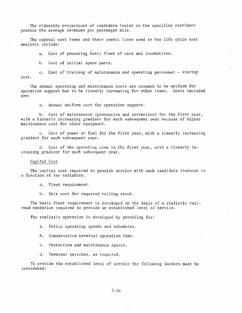
The ridership projections of candidate trains ln the specified corridors provide the average revenues per passenger mile.
The capital cost items and their useful lives used in the life cycle cost analysis include:
, a. Cost of procuring basic fleet of cars and locomotives.
b. Cost of initial spare parts.
c. Cost of training of maintenance and operating personnel - startup cost.
The annual operating and maintenance costs are assumed to be uniform for operation support but to be linearly increasing for other items. Costs included are:
a. Annual uniform cost for operation support.
b. Cost of maintenance (preventive and corrective) for the first year, with a linearly increasing gradient for each subsequent year because of higher maintenance cost for older equipment.
c. Cost of power or fue~ for the first year, with a linearly increasing gradient for each subsequent year.
d. Cost of the operating crew in the first year, with a linearly increasing gradient for each subsequent year.
Capital Cost
The capital cost required to provide service with each candidate trainset is a function of two variables.
a. Fleet requirement.
b. Unit cost for required rolling stock.
The basic fleet requirement is developed on the basis of a realistic railroad operation required to provide an established level of service.
The realistic operation is developed by providing for:
a. Policy operating speeds and schedules.
b. Conservative terminal operation time.
c. Protection and maintenance spares.
d. Terminal switches, as required.
To provide the established level of service the following factors must be considered:
2-26

a, Comparable seats for all trainsets.
b, Comparable consists (coaches, snack coaches),
c. Necessary and sufficient motive power,
The current estimate of unit costs for required rolling stock is obtained from the most reliable source which includes in order of reliability:
a. Historical data or recent purchases in the United States as documented by the trade journals and United States Department of Transportation news releases.
b. Estimated prices from manufacturers for delivery in the United States,
c. Estimated prices from manufacturers for delivery in the country of origin,
For all foreign suppliers being considered in the IPEEP, the following import/tariff rates apply15:
a. , FC' "1 locomotives, both electric and diesel, the rate is 5.5 percent.
b, For'all self-powered passenger coaches, both electric and diesel, the rate is 11 percent.
c. For all locomotive-hauled passenger coaches, the rate is 18 percent.
Maintenance Cost
When evaluating the cost of maintenance of any vehicle, the historical cost of similar vehicles operated in this country should be considered. Electric ~ru car operation in the NEe is a reliable example. Metroliner costs are currently running at approximately $0.85 per mile for servicing and maintenance, but the Silverliner comrrluter vehicles are currently running $1.10 per mile. The difference between the two, of course, is due to the high mileage operated by the Metroliners averaging over 12,000 miles per month cOllipared with the Silverliner at about 3,000 miles per month.
Historical data from the Turbotrain operating between Boston and New York in the early 1970's indicated a very high maintenance cost, caused mainly by the gas turbine powerplant. The annual overhaul of the turbine engines costs somewhat in excess of $45,000 each. With five turbines on the train, the unit maintenance cost was well over $1.80 per car-mile. Other heavy contributors to the high operating cost of this train were tae pendular suspension, single axle trucks, and complicated gear train.
15Tariff Schedules of the Uni ted States Annotated, I :)7().
2-27

Of course, the cost of maintenance will also be greatly influenced by the cost of the spare parts, particularly if manufactured in a foreign country. Metric standards may require special tooling and equipment, and the metric conversion will be slow for properties having rolling stock with a long useful life. Vehicles utilizing metric systems would initially be more costly to maintain during the transition period.
Spare Parts
For conventional units such as electric ~lli cars or diesel locomotives manufactured in this country, it would be relatively simple matter to estimate the spare parts required to keep the units in serviceable condition without undue delays awaiting material. Imported nonconventional equipment will require a different and perhaps less reliable estimate resulting in greater spare stock levels, just to be safe.
If it is necessary to import parts from a foreign country, the acquisition time becomes very important. Parts made in the United States are easily and quickly exchanged by manufacturers (such as General Motors and General Electric), ~nd normally can be shipped from the manufacturer even before the defective unit is received at the plant. This results in a much lower inventory of spare parts than would otherwise be necessary.
The availability of competent service engineers for imported equipment would also have an impact on the inventory of spare parts. With competent field support, the effect of long lead times and high inventories could be partially offset by the ability to make field repair and modifications.
2.9 MODIFICATION FOR NORTH AMERICAN OPERATION
There are five basic areas in which changes may be required. These are:
a. Structural reinforcement to meet Association of American Railroads (AAR) interchange requirements.
b. Propulsion equipment changes for use of 25 kV, 60 Hz.
c. Addition of the Amtrak interiors and specialty items such as the cab signal system.
d. Adaptation of doors and steps for high and low level platforms.
e. Modification of carbodies and/or trucks to meet clearance restrictions imposed by existing corridors.
Each of the trainsets under consideration represents an integral design capable of certain levels of performance. Adaptation to suit United States service operations, particularly the collision strength requirements and attendant weight increases, may completely disrupt the design integrity of the trainset. The adapted design could therefore represent a completely new version at considerable redesign cost.
2-28

The first area, that of structural reinforcement, if of serious concern for all foreign trainsets in the Union Internationale Chemins de Fer (lIIC) buff strength requirements set forth in UIC Code 567-1 OR represent approximately 55 percent of the AAR requirements. The additional stren~th and the weight of such changes could lead to a progression of other changes which affect the performance of the trainset design. These may be described as follows:
Progression of Weight Increases:
a. Primary (cause): Collision strength reinforcement.
b. Secondary (effects): Increased propulsion equipment rating and weight to overcome
weight increases. Increased brake equipment weight to overcome weight increases. Increased truck weight to handle weight increases.
c. Impact of Weight Increases: . Structural:
Additional support for increased size propulsion equipment. Additional support for increased size braking equipment. Additional truck load capacity.
,~erformance:
Additional tractive effort required to handle weight increases.
Additional braking effort required to handle weight increases. (This is a very important factor.)
The simplest approach is to increase the car structural strength and accept L reduction in performance of the propulsion system due to the weight increase of the structure. Depending on the capacity of the trucks, this could be accomplished without a change in truck design. The friction brake capacity, however, would almost ce~tainly have to be increased (or top traIn speed reduced) to handle the energy dissipation and rates requil:ed for signal stop distance.
The second area of change varies widely in its impact on various trainset designs.· This involves the adaptation of the transformer and power collection equipment on ac electric equipment for 25 kV, 60 Hz. Trainsets with dc propulsion requiTe the addition of transformer and rectifier equipment for NEC operation. Diesel or turbine equipment will be unaffected.
Since all the electric propulsion systems employ dc traction motors, changes may be required in solid state power circuits and smoothing reactors to limit ripple from the 60-Hz supply to levels which the motor design will accommodate.
The third area of change includes adaptation of passenger seating and food service to Amtrak standard practice. This generally involves replacing one set of equipment with comparable Amtrak approved designs. Cab signal equipment for the North American corridors involved, would also be required. This too involves replacement of foreign equipment with Amtrak standard devices.
2-29

The fourth area is the adaptation of vestibule floor heights, step wells, and doors for use with both high and low level platforms already in existence throughout the United States. In some cases, devices will be required to bridge the gap between the platform edge and the door sill of the narrower trains.
The last area is the consideration of clearance restrictions imposed by the various North American corridors. While many candidate trains are built to generally more restrictive clearances than North American practices require, the third rail clearance restrictions of the Northeast Corridor represent a severe restriction in the area of trucks and underf100r equipment enclosures. Trainsets built for use on new or otherwise exclusive rights-of-way often conflict with these restrictions.
2.10 CRASHWORTHINESS
The crashworthiness of a rail vehicle can be characterized generally by the overall performance of the unit during and immediately following a collision. For locomotives and freight cars, a primary criterion for crashworthiness is the energy-asorbing capacity of the vehicle's structure. For passenger cars, an additional criterion is the effectiveness of the vehicle's interior design to prevent injuries and fatalities, as well as the ability to protect passengers in trailing cars.
Collisions may be characterized as those between two trains, and those consisting of a train and other vehicles or structures that could cause severe damage and injury upon impact with the train. Train-to-train collisions may be further categorized by the orientation of impacts, i.e., front-to-front, frontto-rear, rear-to-front, rear-to-side, etc. An added characterization describes the behavior of the impacting and impacted units, such as overriding, buckling, crushing, "jackknifing," lateral derailment, and damage done to other cars in the consist. Train-to-nontrain collisions can have one of many configurations.
This segment of the report briefly reviews the existing structural standards for rail vehicles, and general analytical methods for assessing vehicle crashworthiness.
Existing Standards for Crashworthiness
Various transportation agencies have prescribed structural standards for rail vehicles with the objective of defining minimum levels of structural integrity for acceptable protection and safety. In the United States, the Federal Government has adopted a concise set of standards 16 based on those endorsed by the American Association of Railroads 17 that deal essentially with vehicle static frontal strength. Part 230, subpart D of the Federal code applies to self-propelled electric units; the MR recommendations apply to all passenger cars in interchange service, and are summarized in table 2-4.
16Code of Federal Regulations, Title 49 - Transportation, Parts 200-999, U.S. Government Printing Office, Washington, D.C., 1975.
17Specifications for the Construction of New Passenger Equipment Cars, Association of American Railroads, revised 1969.
2-30

TABLE 2-4. MINIMUM REQUIREMENTS FOR RAIL VEHICLE FRONTAL STRENGTH.
Train Weight Train Weight < 300 tons > 300 tons
Buff load, lbs 400,000 800,000 Anticlimber strength, lbs 75,000 100,000 Collision post attachment strength, lbs 200,000 300,000 Truck attachment strength, lbs 250,000 250,000 Coupler carrier truck load resistance,
lbs 75,000 100,000
Definitions of Terms Used in Table 2-4. The terms used in table 2-4 are conventional; however, additional ampiification is provided below:
a. Static end (buff) load. Structure should resist prescribed longitudinal load at rear draft stops ahead of bolster in the draft centerline wi-d. no p'-;rmanent deformation in unit structure.
b. Anticlimbing scheme. Required at each end of unit to prevent relative climbing of two coupled units. Should resist prescribed vertical load without excecUlng yield point of the material.
c. Collision posts. Members located at the outside end of the vehicle, one at each side of the diaphragm opening. Each member should meet or exceed a prescribed ultimate shear strength "at a point even with the tip of the underframe member to which it is attached. The attachment of these members to a bottom shall be sufficient to develop their full shear value."
d. Truck-to-unit body locking. Should exceed 250,000 pounds ultimate shear strength.
e. Coupler carrier and conne(:tions to unit structure. Should resist prescribed downward thrust load from coupler shank without exceeding the yield point of the material.
The general data required to evaluate a rail vehicle with respect to these standards are listed in table 2-5.
Individual transit authorities (e. g., the MBTA, NYCTA, CTA) have developed their ow~ standards, which vary between transit authorities. However, these are based generally on the AAR standards but in some cases are lower because the equipment is operated on properties with dedicated right-of-way.
Duropcan standards for interchange service are specified by the Union InteTnationaLe des Chemins de Fer (UrC) in Paris, France. The UTC standards differ from the AAR interchange standards in several respects. This can create a prob lem for assessing the acceptabi Ii ty of European-built trains to operate in the United States. For example, the UIC's minimum required buff load is less than that of the AAR standards, and generally, UTC standards categorically fall short of the AAR standards, Consequently, unless the European vehicle is overdesigned, it will not meet United States standards for frontal strength.
2-,31

TABLE 2-5. DATA REQUIREMENTS TO ASSESS ACCEPTABILITY OF CANDIDATE TRAINS BASED ON AAR STRUCTURAL STANDARDS.
Category
(1) Car axial strength (max. buff load)
(2) Anticlimbing requirements
(3) Collision-post attachment strength
(4) Truck attachment strength
(5) Coupler carrier requirements
Data Needed
Results of axial load tests.
Material properties, dimensions, and location of structural arrangement at each end that can carry vertical load, and maximum allowable vertical load.
Material properties, dimensions, and location of main vertical members at outside end, on either side of diaphragm (if they exist), Also any reinforcement to the members to add shear strength, and how these members are attached to underframe. Specifically need ultimate shear strengths (longitudinal and lateral) at point of attachment.
Ultimate shear strength of locking means of trucks to unit body.
Material properties and dimensions of coupler carrier, any auxiliary equipment when yielding type of coupler carrier is used, and connections to unit structure. Also need range of positions of coupler in horizontal plane.
Another potential problem is the difference in front-end structural design between some overseas-built vehicles and North American-built vehicles. For example the UIC standards for complex design differ from the AAR standards followed in the United States. Consequently, modifications to the vehicles built overseas may be required to provide couplers and coupler strength compatible with vehicles built in the United States.
Analytical Methods for Assessing Rail Vehicle Crashworthiness
Several levels in the hierarchy of models for assessing rail vehicle crashworthiness exist. These range from a simple-spring and rigid-mass representation of a single car, to a rigid body model of two trains having several cars, to detailed finite element car models. Provided the vehicle parameters, e.g., masses, inertias, stiffnesses, etc., are well defined, the more complex models will describe the behavior of the actual system more accurately. Simpler models
2-32

can be sufficient for identifying trends (as shovffi by Raskin18 ) and performing comparative analyses of several different vehicle designs and crash situations.
As shown by Cassidy and Romeo 19 and Tong,20 the solutions obtained by using different models can vary greatly. Typically, the simpler models will have a conservative upper bound on the severity of a crash, while more sophisticated, and thus more accurate, models will more closely predict the actual behavior and give a lower bound on crash severity.
Typical indicators of vehicle crashworthiness used in analytical studies are the kinetic energy of collision (assuming a perfectly elastic wayside collision), the energy absorbed during impact (by component deformation, wayside damage, heat, and noise, etc.), and the vehicle crash strength, which is inversely proportional to the effective longitudinal strength-to-weight ratio. Although longitudinal strength is emphasized in the AAR standards, severe damage and passenger fatalities typically result from override of one vehicle onto another. The severity of vehicle override is a function of the vertical strengths of the impa"ctim!: cars.
It should be pointed out that a simple stress analysis is sufficient to tlssess whether a particular vehicle will meet the existing AAR standards listed in table 2-4. The models and methods discussed above are valuable to assess more thorougl,1:, the crashworthiness of a vehicle, but generally are not necessary to determine whether the vehicle meets the AAR standards for frontal strength.
18D. Raskin, "Physics of Collision," Transit Development Corporation, Washington, D.C., October 1974, available from National Technical Information Center, Springfield, VA, P8-241-852.
19R. Jo Cassidy, and D. J. Romeo, "An Assessment of the Crashworthiness of Existing Urban Rail Vehicles," Volume I and Final Report to Transportation Systems, Contract DOT-TSC-681, November 1975.
20Pin Tong, "Mechanics of Train Collisions," Final Report, U.S. Department of Transportation Systems Center, Cambridge, MA, April 1976, NTIS PB-258-993.
2-33


APPENDIX A. TRAIN PERFORMANCE MODEL
A.I INTRODUCTION
The train performance program used in this study is part of the CarnegieMellon University (CMU) comprehensive "Energy Management Model", figure A-l. The train performance simulator flow chart is shown in figure A-2. All the important input and output quantities can be displayed in a variety of ways including "character-plots" and "continuous plots." Examples of some of the available displays are shown in figures A-3 to A-S.
A.l.l Program Input
Input to the train performance simulator includes:
a. The physical characteristics of the train, specifically:
o Empty weight.
o Number of passengers (100% load factor).
o Length.
o Cross sectional area.
o Number of axles.
o Powered or non-powered.
o Auxiliary power requirements (KW, KVAR).
o Rotational weight.
b, The performance characteristics of the propulsion system, specifically:
o Number and types of motors.
o . Motor characteristics (voltage, current, frequency vs. torque, speed).
o Number and types of gear units.
o Gear unit characteristics (torque/speed - input/output).
o Number and types of transmission.
o Transmission characteristics (torque/speed - input/output).
o Power control characteristics (input voltage, current and frequency vs. output voltage, current and frequency).
o Equivalent rotational weight.
A-l


,~
N
__
_ '::;
:'V':;:
::::C:
::'A': _
_ "jl
C;o
.a;; 5'JaA~AGE~.mr;.;~~-; M
OO
=:a.
E::·::
:::~>:
:: . r: F·
":"" ""
:.,. "~
BL
OC
K D
IAG
RA
M
"".,
", .
. ""
' .. ,,,
,,,,,,
,,.,,
I ",
,,'c
o, "m
"",
W'"
_
,,,,
,,,,
,,.,
,,,,
,,,,
,.,,
,,,,
,,.,
,,,,
,,,,
, ""
''''''
"'' "
",,""
" : :,
:::.:~
':;::,
:'::::
;:':'"
:':::,
",:,,:
::,,,
, . "' ___
_ 1
'lII
_
__
_
"''''''''''''
''''''''''''''
''''''''''''''
t~
~
--~~
~m~~~~rnB~~~"_~~~~~~=_~_~~~~~:::~~=:::~~~~ru~~~cw~~~~_~~m~~~~~~~~m~m~m~
__ JI
II .. _
__
_ ~
r-~----'
L' :;:;,it~iB\~:
:;:"ii~;~~
.'ir:~@;1~
i: !~
'<""
T"O
''''"
'
. .
'
.""'"''
''''''
''''''
''''''
''''''
''''''
''''''
''''''
''''''
''''~'
'"''''
''''''
'"''''
''''''
'''""m
.,,'
".";;::
;""""'
'''''''':
, .. " "",,, "
,,,,,,,,,,
,,,' .:
";;",.
;~,::,
;::
.. ",,., "i
'"'''''''''
''''''' :::r
P
""""
''''''
''''''
''''''
''' "'
''''''
''''''
''''''
'''~
e 1
~---lJ
::;:';
::;:~:
;i::''
.:':;:
':':''
:::'''
''':;'
:':::'
'''~
r1~,
/.,,,,,,,,,"
,,,,,,,,,,,,
,,,,,,-,,,,,
,,,,,,,",,,,
,,,," t+
--Cc
r-.c--
-I ~ ~ n
"""""''''".,
.. ""
. [
.",,
,,,,
,,
,'
~:~~ .. ' ::
~,t ;',',.
:;:,~ 1,_'
) "
,' ,
',
D
D
~ D
Q
I o o o o U
Q a D c n D
Q n n c n G n ~ n n D o
~.
~"""" .~
'-t
."~
I-l ~
, [
"~,"~;
'f,=::
=i 1.i 0
,,, ,,
"" '
"'' ",
,, ''',
~ '"
''
"'
""
! co
'c,,
,,,,
,.,.
~ ~
J B =
S""
" 1
C
: ,,
,,"'
" :',"
,',,,":
::",,':
'" ;"~
::<~'g
:';:,,
, ';'
,' :
t ,,
,"'''
'0,,
,,,
ft b
,.""
"""·
""",
,,,
"""i
'"
I
~"~:,:
.':':,
:.;:'"
,:~",,
,,,,, ~ _
_ ~ _
_ =
=~~
, ~= ~===~,~~,~~= ==~
o, ~.
<."~
~, C~t
· m ~
',',
-,-~
'" ,
,' ,~
= ,,
~, ,.
-=
'D =
'"
re ~ ~ M~ ~~, ~ =
= ="
,,~,
' '0
=~~
, ==~~ =
= ~_~
~~ =
=~ =,
,~ "
==
==
_ ~ =~, m
~ ~
_.'
.' ::::
:~~~:,
:.::;;
:;~:::
~;'
C
! ;
;~~;~;:o
,eo~;:~~
;.:,:~;~
~~.:,~';
.u"~[,.'
~~.~.~~~
'~~'
D
EL
EC
TR
IC N
ET
lf"O
RK
SIM
UL
AT
OH
A
p
.
~=~= _
_ ~~~~=~===~=~~================~~_~===~=~_~~oo_m _
_ ~ _
__
__
=~ _
_ ==~
~"~~;:J~ IM~;~.r;~;~;";;iW
I [=;::~;~1--
;-~.-'
:=~~"~
~~"~~l
A l,w
'ft'"
1 I ''
'''T''~=
:-: O!
£""i
*"'if
' ,
: :'""
':t· ~ ....... :
... :.:. :.:.: 1]1
r;~
::,--
1""'1
""':,
,~~~~~
:~~?-
:~I~~i~:
:0':
'I~~~:
~ J
L-----
---T:t
~!~.,;
.1 1 _
_ ··
~~~~w~-~=~~=~h"'~==~=~~mG~"'~=~=-~=~ ..
~~~~~~-~-m-~~=-e~~M~=~=M_~ ..
c.d
',"""
'
""",
'".
'c.v
>T
,eH
,CU
,"""<
""A
'
; ;0i;m
t~WJi ;
;;;::"
F /
FIG
UR
E A
1
eM
U E
NE
RG
Y r
-.,jA
NA
GE
l\lE
NT
:l.
l0D
EL
A2


READ INPUT
SUMMARIZE INPUT
INITIALIZE VALUE:S
YES
~ ARRANGE OUTPUT IN
DESIRED FORMATS
')1~:::o§~"i~SUMMARIZE ENTIRE RUN END
1IIiIi __ ,
; I e
REseT STORAGE POINTERS
~ I
V<SPEED RESTRICTION?
HAS TRAIN JUST COME INTO A
NEW SPEED RESTRICTION?
~ RESTRICTION ~
~ t3 ~ __ ~~~~~~~~~~ __ ~~d
NOTES
FORWARD CALCULATION
V IS THE INSTANTANEOUS SPEED OF THE TRAIN
THISSTEP IS PRESENTLY INOPERATIVE; IT
WILL BE ACTIVATED WHEN VARIABLE TIME
INCREMENTS ARE ALLOWED.
m ~ ~ ~ ~ ~ ~ e ~ u U €f==-"'=~9 U ~ o ~ ~ ~ o
V = SPEED RESTRICTION
DISTANCE ~ MILE POST SPEED
RESTRICTION STARTS
~ ~ ~ ~ ~ ~ ~ m ~ ~ ~ n ~ ~ B m ~ ~ ~ ~ ~ W
~ ~ ~ ] ~ ~
~~~-~=-~~~~~ ___ ~~_~B BACKWARD CALCULATION
FIGURE A-2. FLOW CHART FOR THE TRAIN PERFORMANCE SIMULATOR.
A-3

METROLINER WITH REGENERATION MIN TIME
1461 6 TOTAL VEHICLES 6 POWERED BY 4 MOTORS EACH
226.0 MILES TOTAL IN 164 MINUTES AND 39 SECONDS 82.3 MPH AVERAGE SPEED 120.0 MPH TOP SPEED
_ MAXIMUM ACCELERATION IS 1.32 MILES PER HOUR PER SECOND MAXIMUM BRAKING IS -2.07 MILES PER HOUR PER SECOND
ENERGY CONSUMPTION
6.10 KWH / CAR MILE 0.00 KWH / TRAILING CAR MILE 65.95 WH / GROSS TON MILE 0.00 WH / TRAILING TON MILE
IN TIME ) IS 8270.125 KWH 3013.711 KW
11663.461 KW
TOTAL ENERGY CONSUMED IS AVERAGE POWER CONSUMED ( PEAK POWER CONSUMED IS 50.0 KW AUX / VEHICLE 0.0 KW AUX / TRAILING CAR
ENERGY CONPON[~NTS iN KWH
ELECTRICAL ENERGY INPUTED TO THE TRAIN 8270.1 NET INPUT 9503.0 GROSS INPUT
-1265.4 RECOVERED THROUGH REGENERATION
OTHER ENERGY INPUTS -35.5 NET REDUCTION IN TRAINS GRAVITATIONAL POTENTIAL ENERGY
0.0 NET REDUCTION IN TRAINS KINETIC ENERGY
PROPULSION UNIT LOSSES 2521.7 TOTAL LOSSES OVER THE ENTIRE RUN
769.5 LOST IN POWER CONDITIONERS 1752.3 LOST IN MOTORS
0.0 LOST IN GEAR TRAINS 440.5 TOTAL LOSSES DURING REGENERATIVE AND DYNAMIC BRAKING 154.0 LOST IN POWER CONDITIONERS 286.5 LOST IN MOTORS
0.0 LOST IN GEAR TRAINS
OTHER LOSS COMPONENTS 822.7 CONSUMED BY AUXILIARIES
0.0 CONVERTED TO HEAT BY DYNAMIC BRAKE RESISTORS 972.6 CONVERTED TO HEAT BY FRICTION BRAKES
2054.7 LOST TO AERODYNAMIC FRICTION 1746.2 LOST TO ROLLING FRICTION
0.0 LOST TO CURVATURE IN TRACKS 0.0 LOST TRANSFERING INTO AND OUT OF STORAGE
FIGURE A-3. OUTPUT SUMMARY (TYPICAL OUTPUT GENERATED BY THE TRAIN PERFORMANCE PROGRAM).
A-4

METROLINER WITH REGENERATION MIN TIME
1461 6 TOTAL VEHICLES 6 POWERED BY 4 MOTORS EACH
POWERED VEHICLE DATA
92.'5 TON EMPTY 92.5 TON FULL 0.00 LOADING FACTOR AT START 4 AXLES 85.0 F~ET LONG 50. KW AUX
555.0 TON TOTAL TRAIN WEIGHT 110. SQUARE FEET FRONT AREA 36. IN WHEEL DIAMETER 2.4 GEAR RATIO 11000. VOLT
I I I
10 5 -I I I I
Part of the Input Summary (Typical Output Generated by the Train Performance Program)
I * * * * * * * * * * * * * * * * 1** I * * I *
0.5 ~ * I I I I
* * *
* * *
I---1---I---I---I---1---I---I---I---I---I---I---I---I-~-I o 1 2 3 4 5 6 789 1 1 111
o 0 0 0 0 0 0 0 0 0 1 234 o 0 000
ACCELERATION ( MI / HR / SEC ) VS VELOCITY ( MI / HR ) ON LEVEL TANGENT TRACK
FIGURE A-4. PART OF THE INPUT SUMMARY (ACCELERATION VS. VELOCITY).
A-5
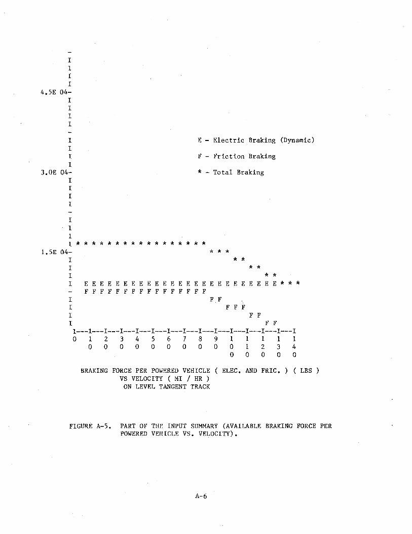
I I I I
4.5E 04-I I I I
I E - Electric Braking (Dynamic) I I F - Friction Braking I
3.0E 04- * - Total Braking
1.5E
I I I I
I I 1 1 * * * * * * * * * * * * * * * * *
04- * * * I * * I * * I * * I E E E E E E E E E E E E E E E E E E E E E E E E E * * *
F F F F F F F F F F F F F F F F I F F I F F F IFF IFF I---I---I---I---I---I---I---I---I---I---I---I-~-I---I---I
o 1 2 3 4 5 6 7 8 9 1 1 III o 0 0 0 0 0 0 0 0 0 1 234
o 0 000
BRAKING FORCE PER POWERED VEHICLE ( ELEC. AND FRIC. ) ( LBS ) VS VELOCITY ( MI / HR )
ON LEVEL TANGENT TRACK
FIGURE A-5. PART OF THE INPUT SUMMARY (AVAILABLE BRAKING FORCE PER POWERED VEHICLE VS. VELOCITY).
A-6

o Control logic.
o Wheel diameter.
c. Vehicle Friction Braking System;
o Friction braking characteristics.
o Friction braking control.
o Electrical/friction brake blender.
d. Transportation System Physical Layout:
o Terminal locations.
o Station locations.
e. Track Profiles:
o Speed restriction vs. position.
o Grade vs. position.
o Curve radius vs. position.
f. Train Timetable:
o Passenger load factor.
o Station dwcll timc.
g. Control Philosophy:
o Acceleration rates.
o Braking rates.
o Cruising speed.
o Coasting initiation and termination.
A.l.2 Program Output
The program output includes:
a. Summary of Input Data:
o Train name.
o Number of vehicles.
o Number of powered vehicles.
A-7

o Empty weight per car.
o Full weight per car.
o Number of axles per car.
o Vehicle length.
o Auxiliary equipment power demand.
o Frontal area.
o Gear ratio.
o Line voltage.
o Wheel diameter.
o Graph of maximum permissible acceleration vs. velocity (on level tangent track).
o Graph of maximum permissible deceleration vs. velocity (on level tangent track).
o Graph of maximum available tractive effort vs. velocity.
o Graph of maximum available braking effort vs. velocity.
o Listings of profile data (optiona1).
b. Calculated Vehicular Trajectory:
() Speed vs. position.
o Time vs. position.
c. Calculated Power and Energy Consumption:
o Total power demand vs. position (including reverse flows if regeneration is permitted).
o Energy consumption vs. position.
o Component power and energy flows, including power conditioner losses, motor losses, gear train losses, rolling resistance losses, aerodynamic and form factor losses, frictional braking losses, dynamic resistor dissipation, regeneration and auxiliary consumption.
d. Summary of Trajectory and Energy Consumption Data:
o kWh/car mile.
o kWh/trailing car mile.
o Wh/gross ton mile.
A-8
a Wh/trailing ton mile.
a kW average.
a kW peak.
a kWh gross.
a kWh net.
a kWh recovered through regeneration.
a kWh lost in each component area.
o Total distance traveled.
o Total route time.
a Average velocity.
a Peak velocity.
o Peak acceleration.
a Peak deceleration.
A.2 PROGRAM PHILOSOPHY
The train performance simulator generates its output with the aid of discretization, numerical integration, and a number of special purpose modules, namely:
TCM: Train Capability Module. Given the train's velocity and position (that is, pervading track conditions) this module determines the maximum acceleration and braking of the train. As such, it identifies, at any selected point along the train's trajectory, the range of acceleration/deceleration immediately available for continuing the trajectory.
1M: Integration Module. Given the acceleration/deceleration to be maintained over a time interval, ~t, and the train's velocity and position at the beginning of ~t, this module calculates the train's velocity and position at the end of the interval, ~t.
POM: Power Demand Module. Given the velocity of the train at any instant in time and the tractive effort developed by its propulsion system, this module calculates the real power (dc line) or complex power (ac line) being supplied to the train.
The TCM and 1M modules are used to generate the speed-position-time-trajectory of the train, subject to the pervading speed restrictions, track conditions, and governing control strategy. The basic steps involved in generating any segment of this speed-distance-time trajectory are:
A-9

a. Begin at a pointfo~ which the position, speed and time are known.
b. Select a time step (time interval), ~ T.
c. Determine the range of tractive effort that the propulsion and braking systems can deliver. (Part of this range will be negative, corresponding to the negative tractive effort available from braking systems. The extent of the range is, of course, speed dependent.)
d. Select a tractive-effort-value that lies within this range and is consistent with pervading speed restrictions and trajectory objectives.
c. Determine the resulting acceleration and compute the train's velocity and posjtion at the end of the time step, ~ T.
f. Repeat steps c through f to advance the traj cctory in time and distance as far as necessary.
The procedure is illustrated in figure A-6.
To determine the entire trajectory, steps a through f are combined with a stratagem that ensures the simulated train slows when and where required. To aid in explaining this stratagem, consider the problem of moving from points A to B in figure A-7. Suppose that the speed restrictions to be met are shown by the broken lines; during accelerating, the train is to use the maximum tractive effort available from the motors, and during braking, the maximum braking rates available.
If the entire trajectory were calculated beginning from point A, it would be difficult to determine the points F and E at which braking is to be initiated in order to meet the speed restriction at point C and to stop at point B. Therefore, the braking portions of the trajectory are calculated "backwards" (with a negative time step) beginning at their terminal points C and B. The points E and F at which the actual train would initiate braking are, then, merely the intersection points of pairs of adjacent forward and backward trajectory segments.
Once the entire trajectory has been generated, the PDM Module is called at selected points along the run to determine the train's demand.
A-IO

FULL THROTTLE OR POWER
~
FULL BRAKING
TIME ==~
-FIGURE A-6. FINITE DIFFERENCE PROCEDURE FOR CALCULATING SEGMENTS OF THE
SPEED~DISTANCE TRAJECTORYo
A-ll

A
" Backward /
Calculation
Forward Calculation (acceleration a~d cruise)
Speed Restriction
" Forward Calculation
Bach/ard / Calculation
(brakinq)
. IlISTAN£L. B
Segments of the speed-distance trajectory and the directions
in which they are computed. Segments AF and CDE are com
puted forwards beginning from the points A and C. Segments
CF and BE are computed backwards beginning from tbe points
C and B. Points F and E represent the intersections of
pairs of adjacent forward and backward segments.
FIGURE A-7. SPEED DISTANCE TRAJECTORY.
A-12

APPENDIX B. SPEED RESTRICTION CALCULATOR FOR CURVES
B.1 INTRODUCTION
The speed at which a rail vehicle can negotiate a curve depends not only on the curve characteristics, but also on the vehicle's design. In general, a curve is well defined by its steady-state superelevation and curvature, and the length and type of the entrance and exit spirals. Assuming that the spiral is designed to provide gradual transition between the tangent track and the steadystate part of the curve, the critical length of track is the steady-state section. In any detailed analysis of the vehicle's dynamics, it is necessary to conside r the influence of the off-nominal track conditions which do exist t.o a greater or lesser degree depending on track maintenance. However, because of the complexities involved, no attempt has been made to include track imperfections in this model. Therefore, track limitations are defined only by the curve's superelevation and curvature.
B.2 CRITERIA
i'he most commonly used speed restriction in a curve is unbalance speed. T!le unbalance is actually the superelevation deficiency which, when added to the actual track superelevation, would provide an equilibrium condition between gravi tationa 1 0~rl centrifugal forces in the lateral p lane of the carbody.
lfc:hic1e characteristics are not necessary to define unbalance speeds because such speeds are only a conservative first-order limitation which are independent of the vehicle. The justification for using a maximum of 3-inches unbalance is based on tests performed over 25 years ago. ,The results of these tests determined that most passengers were comfortable if the lateral force in the curve was equivalent to less than 0.1 g. Theoretically, 0.1 g lateral acceleration is produced at about 6-inches unbalance if th~ suspension systems are rigid. If the secondary suspension is very soft, as it was for many passenger trains before 1960, t~1e carbody will undergo a relatively large roll displacement in a curve, subjecting the passenger to greater lateral forces. Typically. 0.1 g was developed with an unbalance of between 4 and 5 inches. As a result, 3-inches unbalance was established as a lower bound, allowing for the carbody's roll characteristics to effectively produce the equivalent of at most 0.05 g when the track structure and speed already produces 0.05 g indepe:ndent of the vehicle.
But with today's high-speed passenger trains, the roll suspension is very stiff, allowing vehicles to negotiate curves at unbalances near 5.5 inches without exceeding 0.1 g lateral acceleration on the passenger. Therefore, if the comfort limit is defined as 0.1 g lateral acceleration rather than 3-inches unbalance, speeds in curves can be increased substantially. The maximum lateral acceleration on the passenger is then a second criterion of speeds in curves. Since it is necessary to know the roll characteristics of the particular vehicle to determine the actual lateral acceleration experienced by the passenger, vehicle weight, suspension stiffnesses, and component geometries are required to calculate speeds which produce a given maximum lateral acceleration.
B-1

The third curving criterion considered in this model was the one-third rule which states that the resultant load vector due to the centrifugal and gravitational forces must be within the middle third of the distance between the rails. As can be seen, this is an overturning stability criterion. There is, however, some room for interpretation of the middle one-third distance of the track. Loosely taken the effective gage is approximately 60 inches, so the one-third distance would be 10 inches either side of the center of the track. However, a much stricter definition has been advocated by some. The argument is that the actual measured gage is 56-1/2 inches, which essentially decreases the half gage from an effective value of nearly 30 inches to one of 28-1/4 inches. Another conservative criterion states that the load vector due to gravity and centrifugal forces must lie within 8-1/4 inches of the track centerline. As in the case of calculating the curving speed at which the lateral acceleration of the passenger is a specified value, vehicle parameters such as weight, stiffness, and geometry are also needed for the one-third rule.
Two special effects are also incorporated into the model. First, a limit on the relative displacement between the carbody and the truck frame is specified. This extra consideration will provide both a higher speed for the onethird rule and for the maximum passenger lateral acceleration if the limit is reached. A second additional feature to the model is the active roll of the carbody. The primary effect of rolling the carbody is to reduce lateral acceleration on the passengers when negotiating curves at high unbalances, i.e., 6 to 9 inches. If the active roll center is below the carbody center of gravity (eg) the carbody will be displayed toward the inside rail. This results in the load vector from the carbody cg also being shifted inward. The result is that a higher speed can be tolerated for the one-third rule.
Both the maximum stroke in the secondary lateral stiffness and the carbody active roll are nonlinear effects and require an iteration scheme in the computer model. But even with the iteration loops, the simulation is very inexpensive.
B.3 NOMENCLATURE
al aZ D dl dZ d3 d4 d6 E
Fc G gmax go Kxp Kxs Kzp Kzs K~s R U
Wc
(half lateral separation of primary vertical stiffness) (half lateral separation of secondary vertical stiffness) (degree of curvature) (height of primary lateral stiffness above wheel/rail interface) (height of truck frame cg above wheel/rail interface) (height of secondary lateral stiffness above wheel/rail interface) (height of carbody cg above wheel/rail interface) (height of act~ve tilt roll center above wheel/rail interface)
. (superelevation of steady-state curve) (centrifugal force acting on cg of carbody) (effective wheel/rail gage) (specified maximum lateral g load on passenger) (acceleration of gravity) (primary lateral stiffness - per axle) (secondary lateral stiffness - per truck) (primary vertical stiffness - per axle) (secondary vertical stiffness - per truck) (secondary auxiliary roll stiffness - per truck) (radius of curvature) (vehicle unbalance in curve) (carbody weight)
B-2

WTP (truck frame weight) XA (lateral displacement of carbody cg due to active tilt control) Xc (lateral displacement of carbody cg due to gravitational and
centrifugal forces) Xcm (maximum stroke of secondary lateral springs) Xm (lateral distance from center of track to carbody load vector) Xv (lateral displacement of carbody total load vector at the track plane
due to gravitational and centrifugal forces) a (angle between carbody weight vector and carbody total load vector) 8 (angle between carbody weight vector and perpendicular to track plane) o (clearance between wheel flange and rail) ~ (roll angle of carbody with respect to normal to the plane of the
track due to gravitational and centrifugal forces) ~A (roll angle of active tilt control)
B.4 DERIVATION OF EQUATION
To keep the analytical model relatively simple but still meaningful, only two degrees of freedom were considered: carbody roll and carbody lateral. Before considering the actual vehicle, the following e~pression was used to compute the vehicle curving speed based on unbalance and track characteristics.
(B-1)
The program computes the vehicle curving speed for U = 0, 3, and 6 inches.
To calculate curving speeds which satisfy the one-third rule, a simplified model as depicted in figure B-1 was used. Summing the lateral steady-state forces on the carbody:
(B-2)
Summing the moments about the carbody cg:
° (B-3)
The secondary vertical spring constant, Kzs ' includes the effect of the secondary auxiliary roll stiffness.
Since only two degrees of freedom were used to simulate the vehicle's steady-s~ate configuration, the following equations modified the vehicle suspension and the truck frame in the one-third rule analysis.
B-3

FIGURE B-1. CAR BODY MODEL FOR ONE-THIRD RULE.
B-4
Kzs -- 2

The primary and secondary lateral springs acting in series yield a modified (indicated by the "bar" over the symbol) secondary lateral spring.
Kxs = (Kxs) (2 Kxp)
Kxs + Kxp
Likewise, for the vertical springs:
K = zs
(Kzs) (2 Kzp) K + 2 K zs zp
The modified weight of the carbody includes the two truck frames.
Wc = Wc + 2 WTP
(B-4A)
(B-4b)
(B-S)
The effective half lateral separation of the primary and secondary vertical springs acting in series is:
K zs 2 K zp
(B-6)
The effective height above the W/R interface of the primary and secondary lateral spTings acting in series is:
K xs 2K xp
(B-7)
The effective height of the combined carbody and truck frames cg above the W/R interface is:
Wc d4 + 2 WTF d2 Wc 2 WTF
(B-8)
Using -::he above modified parameters and solving equations (B-2) and (B-:n simultaneously yields:
(Cf4
- (3
) (F - W 8) ¢
c c =
2 K a 2 (B-9)
zs 2
r - W 8 (d4
_ d )2 (F - W 8) c c + 3 c c X c 2 K 2 K a 2
(B-IO) xs zs 2
B-5

Now consider the lateral displacement of the load vector from the track centerline is the vehicle suspension is rigid. From figure B-1:
and
tan a = F..;wc c
tan (a - e) = X~
Using the trigometric identify:
tan (a - e) = tan a. - tan e
1 + tan a. tan 8
and equations (11) and (12) produces:
G F - E W c c
G W + E F c c
(B-ll)
(B-12)
(B-13)
(B-14)
The total lateral displacement of the load vector with respect to the track centerline is:
x = X + X + 0 m c v (B-15)
Substituting equations (B-IQ) and (B-14) into equati..on (B-15):
F - W e (~4 - d3)2 (Fc - W 8) X
c c + c = (B-16)
m 2 K 2 K a 2
xs zs 2
C_Fc - E W ) + d4 c + 0
GW + EF c c
Rearranging equation (B-161 results in a second order algebraic equation in F of the form: c
A F 2 + B F + C 0, c c
where A E (COEFF)
W (G2 - E2) COEFF B d4 G - E (X - 0) c
+ m G
C - - G W (X - 0) - E W d4
- E W 2 COEFF c m c c
B-6
(B-l7)
(B-18)
(B-19)
(B-20)

where
1 COEFF = "2
Solving for 1:; •
" c'
F c
-8 ± 182 - 4 AC 2 A
(B-2l)
The vehicle curving speed based on the one-third rule can now be computed.
(B-22)
The effect of the active carbody tilt on the vehicle curving speed must also be considered. Unless the carbody cg and the active roll center coincide, the carbody cg will be laterally displaced due to the active roll of the carbody. The displacement of the carbody cg is:
(B-23)
The vehicle curving speed and the active carbody roll are dependent on each other because the active control will attempt to eliminate the lateral acceleration. Therefore, an iterative computation is necessary to determine the vehicle curving speed.
Solving for the unbalance (U) in equation (B-1) and substituting in the vehicle curving speed from the one-third rule computation above, equation (B-22), an initial ~A is calculated:
(B-24)
Equation (B-15) is then modified to include the effect of equation (B-23) and a new vehicle curving speed is computed, equation (B-22). The procedure is continued until two consecutive speeds are within 0.5 mi/hr of each other.
Secondary suspension stops also limit the lateral travel of the carbody. If the carbody hits against the stops, the effective lateral spring constant is altered.
B-7

To determine the changed lateral spring constant, equation (B-IO) is solved for Kxs when setting Xc equal to the maximum stroke of the secondary lateral
"springs, Xcm . A second i terati ve computation is now necessary to calculate the vehicle curving speed since the vehicle speed, equation (~-22), and the altered spring constant, Kxs ' are dependent on each other.
The vehicle speed based on the maximum lateral acceleration experienced by the passengers is computed as:
v = rR go (gmax + sin (8 - ~))] [ cos (8 - ~) (B-25)
This computation is also an iterative process since ~ varies with the vehicle speed.
B.5 COMPUTER RESULTS
For every curve, the one-third rule speed and the track speed restriction are compared to each other and to either the 3~inch or 6-inch unbalance speed, depending on the vehicle suspension (passive or active, respectively). The corridor data and the vehicle curving speeds or tangent track speed are printed at each selected milepost. The most restrictive speed for each milepost is "flagged" on the printout and is stored in the computer. The set of restrictive speeds can be punched onto cards along with their corresponding mileposts and speed restriction designations for use in the Train Performance Calculator (TPC), or another set of vehicle parameters can be read. If another set is read, the vehicle curving speeds are computed and printed along with the corridor data as before.
The set of restrictive speeds for the new vehicle is compared against the set from the previous vehicles and the lowest restrictive speeds are stored. This comparison is continued until an input parameter requests a deck of cards for the TPC to be punched. After the deck of cards is punched, more vehicle parameter sets can be read, and the above process is repeated until all the parameter sets have been read.
A flow chart for the computer program which calculates the speed restrictions on curves is given in figure B-2.
B-8

t::d I
\..0
RE
A]
CO
RR
iDO
R
DE
SC
RIP
TIO
N
IF M
I L
EP
QS
T C
OR
RE
SP
ON
DS
T
O A
CL
iRV
E
CA
LC
UL
AT
'= 0
, 3,
AN
D 6
· IfI
<CH
UN
BA
LA
NC
E S
PE
ED
S
DD
ES
T
RA
CK
SE
CT
ION
C
OR
RE
SP
ON
D T
O A
C
UR
VE
NO
FIG
UR
E B
-2,
ITE
RA
TE
ON
ON
E-T
HIR
D R
UL
E S
PE
ED
IF
V
EH
ICL
E H
AS
A
CT
IVE
TI
LT
CO
NT
RO
L
ITE
RA
TE
ON
O
NE
-TH
IRD
RU
LE
SP
EE
D I
F
CA
RB
OD
Y
[S A
GA
INS
T L
AT
ER
AL
ST
OP
S
CA
LC
UL
AT
E S
PE
ED
B
AS
ED
ON
M
AX
IMU
M P
AS
SE
NG
ER
L
AT
ER
AL
AC
CE
LE
RA
TIO
N
DO
ES
V
EH
ICL
E H
AV
E
AC
TIV
E T
ILT
C
ON
TR
OL
YE
S
CO
MP
AR
E 6
-iN
CH
UN
BA
LA
NC
E
SP
EE
D,
MA
XIM
UM
PA
SS
EN
GE
R
LA
TE
RA
L A
CC
EL
ER
AT
ION
SP
EE
D
ON
E T
HIR
D R
UL
E,
SP
EE
D,
AN
D T
RA
CK
R
ES
TR
ICT
ION
SP
EE
D T
O
DE
TE
RM
INE
CU
RV
E S
PE
ED
-~-
CC
.1.P
AR
E 3
-IN
CH
UN
BA
LA
NC
E
SP
EE
D,
MA
XIM
UM
PA
SS
EN
GE
R
LA
TE
RA
L A
CC
EL
ER
AT
:ON
SP
EE
D
ON
E T
HIR
D R
UL
E,
SP
EE
D,
AN
D T
RA
CK
R
ES
TR
ICT
ION
SP
EE
D T
O
DE
TE
RM
INE
CU
RV
E S
PE
ED
-] W
RIT
E T
RA
CK
SE
CT
ION
D
ES
CR
IPT
ION
AN
D S
PE
ED
R
ES
TR
ICT
ION
S A
T E
AC
H
1 M
ILE
PO
ST
. [:
LA
G M
INIM
UM
L
SP
EE
D
IS
AN
OT
HE
R V
EH
ICL
E
TO
BE
CO
MP
AR
ED
O
N S
AM
E
.cO
RR
IDO
R
NO
DE
TE
RM
INE
WH
ICH
V
EH
ICL
E P
RO
DU
CE
S
LO
WE
ST
SP
EE
D
RE
ST
RIC
TIO
N
YE
S
FLOW
CHA
RT
FOR
SPEE
D
RES
TRIC
TIO
N C
ALCU
LATO
R IN
CU
RVES
,


APPENDIX c. TWO-AXLE STEADY-STATE CURVING MODEL
C,l INTRODUCTION
The development of the equations of motion for the steady-state curving of a two-axle rigid-frame truck has followed an evolutionary course from a basic, completely linear model with no flanging to the present model which incorporates nonlinear phenomena such as flanging forces, creep forces as a function of wheel load, maximum creep force as a function of adhesion coefficient, and lateral secondary suspension stops, Additional options include aerodynamic wind load, buff load, and active tilt control. Figure B-1 displays the various vehicle parameters necessary to use the computer program.
The Gutputs of the computer code include an itemization of individual forces acting at each wheel/rail interface, plus a summation of the forces for each wheel and each axle. Also, L/V's for each wheel and each side of the truck were calculated. Finally, the load ratio on each side of the truck is computed.
c. 2 NOMENCLATURE
ai .L
a2 Dkj
(later-al distance from wheelset cg to primary longitudinal stiffness of ith wheelset, i = 1,2) (latelal. 0~3tance from wheelset cg to primary vertical stiffness of ith wheelset, i = 1,2) (lateral distance from wheel set cg to wheel/rail interface - half gage) (lateral distance from carbody cg to secondary vertical stiffness) (longitudinal distance from truck frame cg to primary lateral stiffness of Ith wheelset, i = I, 2 - positive if stiffness is forward of truck fr:!lJlf; cg)
([ollgitudin:ll dist:lllce from whcelset cg to primary IlItl'ru\ stirrllt1!'ls of ith wheelsct, i = 1, 2 - positive if stiffness if forward of wheel set cg) (longitudinal distance from truck frame cg to ith wheelset cg, i = 1, 2 - positive if wheelset is forward of truck cg) (longitudinal distance from carbody cg to truck frame cg - positive for front truck, negative for rear truck) (longitudinal distance from carbody cg to truck frame centerplate -positive for front truck, negative for rear truck) (veTtical distance of secondary lateral stiffness above wheel/rail interface) (vertical distance of truck frame cg above wheel/rail interface) (ve:rtical distance 9f carbody cg above wheel/rail interface) (vertical distance of carbody center of pressure (cp) above wheel/rail interface) (ve:ctical distance of buff force above wheel/rail interface) (vertical distance of active carbody roll center above wheel/rail interface) (veTtical distance of primary lateral stiffness above wheel/rail interface of ith wheelset, i = 1,2)
C-l

(') I N
TR
UC
K F
RA
ME
~------------r----
____ , C
EN
TE
R O
F G
RA
VIT
Y)
/Ky
p
an I
CA
RB
OD
Y
-L7
CE
NT
ER
OF
GR
AV
ITY
CA
RB
OD
Y
CE
NT
ER
OF
PR
ES
SU
RE
~_-+_---.
TR
UC
K F
RA
ME
C
EN
TE
R O
F
GR
AV
ITY
CA
RB
OD
Y
CENTEROF~
GR
AV
ITY
'@
."
\ }
I '--W
HE
EL
SE
T/T
RA
CT
ION
MO
TO
R
CE
NT
ER
OF
GR
AV
ITY
-b
k4
CA
RB
OD
Y
AC
TIV
E
RO
LL
CE
NT
ER
-~
11_}
l' -1
I
d 4
d31~
t t ~
ds
I
,
i ..
b7
..I
FIG
URE
C-l
. V
EHIC
LE M
ODEL
FO
R ST
EAD
Y-S
TATE
CU
RVIN
G OF
A
TW
O-AX
LE
RIG
ID-F
RAM
E TR
UCK.
Kxs
Kzs
Kxp

(superelevation of rail) (buff force in lateral direction active at coupler - positive if buff, negative if draft)
Fc (centrifugal force of carbody in steady-state curve) FN(normal aerodynamic force acting on carbody side surface) FIl,F22 (longitudinal and lateral creep coefficient, respectively) lCri (lateral rail stiffness for each wheel, i = 1,2,3,4) Kxp (primary lateral stiffness - per wheel set) Kyp (primary longitudinal stiffness - per wheelset) lC zp (primary vertical stiffness - per wheelset) Kxs (secondary lateral stiffness - per truck) Kzs (secondary vertical stiffness - per truck) l~s (secondary yaw stiffness - per truck) K~s (secondary auxiliary roll stiffness - per truck) Pa (lateral component of centrifugal plus gravity force acting on wheelset) Pc (lateral component of centrifugal plus gravity force acting on carbody) 1\ (lateral component of centrifugal plus gravity force acting on
R
1'0
TORQS w
tTuck frame) (steady-state radius of curvature) (wheP,l contact radius with wheelset in neutral position) (constant yaw torque on truck frame) (axle load) (weight of carbody) (lateral displacement of front and rear wheelsets, respectively -positive, out from center of curve) (lateral displacement of carbody - positive, out from center of curve) (lateral displacement of truck frame - positive, out from center of curve) (effective wheel/rail conicity) (flange clearance between wheel and rail) (active roll angle of carbody - positive, top in toward center of curve) (carbody roll angle - positive, top in toward center of curve) (truck frame roll angle - positive, top in toward center of curve) (yaw angle of front and rear wheelsets, respectively- measured positive from rC'.dius of curve, yawed into curve) (yaw angle of truck frame - measured positive from radius of curve, yawed into curve)
C,3 EQUATIONS OF MOTION
The steady-state equations of motion for a two-axle rigid-frame truck are written in full detail below. Refer to figure C-l and the nomenclature in paragraph C.2, for definition of each variable.
C-3

Truck Yaw - 'l't
{KXp [b~l + b~2J + Kyp [a~l + a~2J + KljiS} ljit + (-Kxp [bkl(d2-dkl)
+ bk2 (d2-dk2]) 4t + {-Kxp[bkl + bk2J) Xt • {-Kxp [bkl bk~
- Kyp [a~lJ}al + {-Kxp h2 bkS J -Kyp ["i2J}a2 + { Kxp [bkl]) Xai
Truck Ro 11 - <P t
{-Kxp hI (d2-dkl) + bk2 (d2-dk2)Dwt + {Kxp [ ~2-dkl) 2 + (d2-dk2) 2J
+ Kzp ["i4 + "isJ}t + {Kxp [(d2-dkl) + (d2-dk2)J) Xt +xp [bk4 (d2-dkl)DWa1 + {Kxp [ bkS (d2-dk2)]Wa2
+ {-Kxp h-dkl ]}al + {-Kxp h-dk2 J}a2
+ t [pc (d3-d 2) + FN (d4-d 2) + 2 FBL (ds -d2) ] = 0 (C-2)
C-4

Truck Lateral - Xt
tKxp hi + bkZ]"t {Kxp [(dZ-dkl) + (dZ-dk2 )].t (+ 2Kxp) Xt + (Kxp [bk4 J)1Val +(Kxp [bkSJ) 1Va2 + fkxp) Xa1
+ tKxp} Xa2 +} rc + FN + 2 FBLJ
Front Wheelset Yaw - '¥al
- p = 0 t
(C-3)
tKxp hi bk4J -Kyp [aflJ} "t {\p h4 h-dkl)J}t {Kxp [bk4J}t ;txp ~~4~ + kyp [a~lJ -wAa1} "al + (-Kxp h4 J zf;~aaA}al ... , 2f) ar J +€xp [b~4J + Kyp [a~lJ) :1 = 0 (C-4l
Rear Wheelset Yaw - '¥a2
[a~Z J}t + Gxp hs (dz-dk2)]) 0t {Kxp [bkS ]Xt [b~s J + Kyp [aiz J -WAa 1 ) "a2 + (Kxp [bkS] Zfl;:lA Xaz)
[a( ] + (Kxp [b~s J + Kyp [at 2 J):Z = 0 CC-5}
Front Wheelset Lateral - Xal
l ± crJ = 0 (C-6)
C-5

Rear Wheelset Lateral - Xa2
1Jia2 + {Kxp + 2~W1A} xa2 -Pa + rKr2 + Kr3] [Xa2 ± a] = 0 (C-7)
In the wheelset lateral equations of motion (C-6, C-7) the lateral rail stiffness terms (Kri) are zero unless the wheel set is flanging the inside or outside rail, and then only one Kri has a value depending on which wheel is flanging. The "_II or "+" sign in front of the variable a in equations (C-6) and (C-7) corresponds to flanging the outside rail or inside rail, respectively.
(C-8)
(C-9)
As an example, the lateral force on the outside front wheel is calculated as follows:
F . W1X
where
1/2 WA
(C-10)
= the product of the rail lateral stiffness and rail lateral displacement (nonzero only when wheel is flanging)
the lateral static wheel force
= the lateral creep force
the lateral gravitational stiffness force.
Vertical forces on the wheels are determined by summing moments about each wheel/rail contact point, and include the wheelset, truck frame, and carbody weights and centrifugal forces, the aerodynamic force on the carbody, and the force due to buff load.
C.4 COMPUTER MODEL FLOW CHART
A flow chart for the computer program which calculates the rail curving forces is given in figure C-2.
C-6 , ... .,...'

CALCULATE CARBODY STEADY -STATE DISPLACEMENTS
CALCULATED CREEP COEFFICIENTS BASED ON STEADY- STATE
DISPU'.CEMENTS OF CARBODY
! --- -=""=~~-~-~.~-~'-~~--_-d===o
SOLVE SEVEr" SIMULTANEOUS ALGEBRAIC EQUATION FOR STEADY-STATE DISPLACEMENTS
r 0)
.S2 SELECTNEXT]
FLANGE CONDITION
CALCULATE WHEEL/RAI L FORCES
NO
r-~~~ST- ~'''''R''"''"E=E=P==;' I COEFFICIENTS )~~,-,-- --
CALCULATE AND PRINT FORCES AND RATIOS
YES
G0 FLOW CIIART I:OH STEADY -STATI: CURVING PROGRAM FOR TWO-AXLE RIGID-FRAME TRUCK.
C-7


APPENDIX D. RIDE QUALITY MODEL
D.l INTRODUCTION
Several ride quality criteria are in current use by different railroad administrations in various countries to quantify passenger ride comfort and to correlate measurable values of acceleration with a subjective index of quality. A frequency-domain, random vibrations model of a rail vehicle was therefore developed to evaluate ride comfort criteria and to quantitatively establish values of ride quality for existing passenger trains.
D.2 RAIL VEHICLE MODEL
For this study a linear, lumped-parameter model was used to represent the rail vehicle. Since in a linear model the vertical/pitch modes are for practical purposes decoupled from the roll/yaW/lateral modes, two separate sets of equations of motion were evolved for these two modes. The resulting separated models cLre shown in figures D-l and D-2 each consisting of seven degrees of moti~;:i freedom. Equations of motion for each system of springs, dampers, and masses were written and then modified by LaPlace transform techniques to algebraic equa-~ions in the frequency domain. The resulting equations were programed for soluti;)]l by matrix inversion a!1d multiplication using available library routines, Thls current program version is called TRKVPSD MOD IB.24
As shown in figure O-J, the vertical portion of the model includes seven degrees of freedom: the pitch and bounce rigid-body modes of the c;lfl>ody, the VOl-tical motion of the sprung mass of the trucks (truck frame and bolster, plus portions of traction motors, where powered), the vertical motion of the unsprung muss of tIle front truck (wheelsets and a portion of the traction motors, where powered), the first vertical bending mode of the carbody (using the mode shape of a free-free beam), and the vertical motion of a midcar suspended mass (the Metroliner transformer, for example). To eliminate one degree of freedom, the rear truck unsprung mass was neglected and the truck primary suspension and track impedance were combined as two complex impedances in series.
Lateral and roll motions are, of course, coupled, and therefore a further simplification to reduce the number of degrees of freedom \vas necessary. The dynamics O:i~ only the front truck masses were included in detail, based on the premise that the carbody represents a good low-pass filter isolating the dynamics of one truck from the ether. The rear truck, therefore, was represented as complex impedances in lateral and roll. In the roll/yaw/lateral model, figure D-2, the three rigid-body motions of the carbody, plus roll and lateral motions of both the front truck sprung and unsprung masses were combined for a total of seven degrees of freedom. Oscillatory modes in the lateral plane commonly referred to as "hunting" have not been considered in this particular model, and it is assumed that all vehicles are operating well below the critical speed of truck hunting.
24 0 . R. Ahlbeck and G. R. Doyle, "Comparative Analysis of Dynamics of Freight and Passenger Rail Vehicles," Summary Report on DOT-FR-20077, Report No. FRA/ORD-77!04, November 1976.
D-l

TRUCK FRAME
q(x,t)
___ 8c(.t) ----
--r----:-==-= ........ -- -S- - -- -t
TRANSFORMER
_~-ltZR
I~·~------------LT--------------~~~l
CARBODY
SECONDARY SUSPENSION
TRUCK FRAME
PRIMARY SUSPENSION
WHEEL/AXLE
TRACK IMPEDANCE
TRACK SURFACE GEOMETRY
FIGURED-I. VERTICAL (PITCH/BOUNCE) MODEL OF RAIL VEHICLE.
D-2

OVERALl.. R!:AR TRUCKIM,oEDANCE (SHEAR, TORSION)
z'~ R
CARBODY
SECONDARY SUSPENSION
TRUCK FRAME
PRIMARY SUSPENSION
WHEELS, AXLES, TRACK
TRACK IMPEDANCE
TRACK GEOMETRY INPUT
FIGURE D-2. LATERAL/ROLL/YAW MODEL OF RAIL VEHICLE.
D-3

Track geometry inputs at the trucks were modified by the "chordal transfer function" to account for in-phase (bounce) and out-of-phase (pitch) motion due to the relationship of track geometry and wavelengths and the axle: spacing. Track geometry inputs at the rear truck of the vehicle for both the vertical and roll/yaw/lateral models were phase-shifted by the truck spacing. In-phase, the quadrature components were calculated and entered in the real and imaginary i~put matrices, respectively:
where:
E* = E (cos 2nLT/A - j sin 2nLT/\),
E* = generalized input at rear truck E = generalized input at front truck LT truck spacing (front to rear centerline) A = truck geometry wavelength j =V-1
D.3 TRACK GEOMETRY INPUTS
A realistic input, or "forcing function,1I is as important in mathematical modeling as an accurate and realistic rail vehicle model. Track geometry irregularities -- rail surface, alignment, track cross level, gage -- have been found to have random distributions of amplitude and wavelength that can be described in the power spectral density (PSD) format of "power" ('in:!./cycle/ft) versus frequency (cycle/ft). Superimposed on these random geometric variations are discrete spectral components that result from other constructional peculiarities.
A number of investigators have found that track irregularities, in common with road and runway surfaces (at least over a limit range of wavelengths), exhibit a random variation in amplitude and wavelength of the form,
By assuming the track geometry to be a stationary random process (at least for a reasonable time period) over a broad frequency range with a Gaussian amplitude distribution, the response spectrum of each output variable may be calculated.
where:
PoCf) = iH(f)i 2 Pi (f) (for a single input)
PoCf) Pi (f)
f \ V
H(f)
output spectrum, G2/Hz track geometry spectrum, in2/Hz
= Pi(A)/V frequency, Hz geometry wavelength, ft vehicle speed ft/sec
= vehicle transfer function Cinput to output)
D-4

By use of a random input, all phase information is lost between the different inputs> unless cross-power spectra are also generated. Note, however, that for a rail vehicle the phase relationship of the same input at the different axles must be maintained as a function of wavelength and axle (or truck) spacing. In the preliminary review, cross-power spectra have not been included, and a simple mean-square addition of the output spectra of a variable due to more than one input has been used for an overall resulto
Recent surveys (1974 to 1975) of the NEC track (under the RG-125 and RG-145 test series) using the DOT Track Geometry Car T-3 have been analyzed, and a representative set of PSD plots have been generated (figure 0...,3)0 The geometry inputs are mechanized on the computer by a two-slope, or bilinear, PSD representing the random background, plus the first four harmonic peaks of the 39-foot Tail length.
Do 4 COMPUTER MODEL FLOW CHART
FiguTe D--4 displays the flow chart for the ride comfort computer program discussed ccboveo
DoS COMPARISON OF PREDICTED AND MEASURED DATA
A comparison of one-third octave band rms accelerations over one truck of a !v1etroliner (cuJ.. (25) is given in figure D-S. The test data are over four 1-mi 1. e track sections on the NEC between Baltimore and Wi lmington. 25 The computer result::.: are from the frequency domain program TRKVPSD, using nominal (as-built) vehicle parameters. A very strong vertical acceleration response is noted between 10 and 20 Hz. It was first thought that aged Pirelli springs (a coil encased in elastomeric material) in the primary suspension might account for this effect. The triangular computed data points show the primary suspension with twice the nominal stiffness and one-fifth the nominal damping 0 The close correlation of the triangular computed data points with the test data for the vertical acceleration is evidence that the primary suspension has aged and stiffened on this car. 1be predicted lateral acceleration between 10 and 20 Ilz did not respond as well to the assumed stiffened primary suspension. This resonance must therefore result from a degree of freedom (perhaps a worn traction motor mount or a localized body resonance) not included in the model.
The overall predicted shape of both the vertical and lateral accelerations agrees quite well with the measured data. However, the magnitude comparisons at some frequencies are less than desired. These discrepancies can be attributed to:
a. The test data were acquired from runs over given sections of NEC track, whereas the rail profile inputs to the computer code were representative of other sections of NEC track.
25F. E. Dean, "Second Comparative Ride Quality Test of Metroliner Cars in Revenue Service," report by LTV Aerospace Corp. under Contract No. DOT-FR-I003S, June 29, 1976.
D-S / /

Iu.
--UJ ...J ()
>()
N Z
~,
!', "
H) 2
3
10 4
1000
"-\
.. '\
\
1\ 1\ \ \
\
1', : ... ~\
'.-. \ ~ \
~ \,
r\ " ... "
\
" '"
100
J J I ,
SURFACE
-- - ALIGNMENT
~-_QI!D 1-- CROSS LEVEL
rv f\ i\','
\\ \\ j~
\ \ \ \~\
\ ~\ \"'1 J.
\. \' \ I
~IJ \ \ 1 \
\ \ \L\
, , \ \
\
\J~ ,
\
Y \' \ \
'\1\ \
\ \
\ \ '\ \
\~ \ \ \
\\ \ , \
\ \ \
10
FT / CYCLE
FIGURE D-3. TRACK GEOMETRY POWER SPECTRAL DENSITIES REPRESENTATIVE OF NORTHEAST CORRIDOR TRACK -- USED AS INPUTS TO RAIL VEHICLE SIMULATION MODEL.
D-6

I READ/WRITE I INPUT DATA
~-~Tc------J
DO LOOP FOR SPEED
c_cc -r---1- DO LOOP
L~:::;QUENCIES
1---C-:j\L-~J-;qTE ! MJWRIX LATERAL \ MODEL L ________ , ___ ----1
l~-~-- __ 'c_~ i CALCULATE \ MATRIX VERTICAL I MODEL L
1 DO LOOP
FOR TRACK GEOMETRIC
_,_=1 CALCULATE
!RACK GEOMETRIC [
~
VALUES
1 CALCULATE
COMPLEX
L VARll\BLES
I -
END DO LOOPS
I
GENERATE FREQUENCY
AND OCTAVE
OUTPUTS
PRINT OUTPUT
FIGURE D-4. FLOW CHART FOR RIDE COMFORT PROGRAM.
D-7

.04 ISO REDUCE COMFORT LIMIT
COMPUTED RESU L TS
I t!J
z .03 0 4HR f= I <C 0: UJ ...J UJ u
.02 u <C '-CJ)
~ 0::: ...J <C u I- .01 0::: UJ >
o L-____ L-____ L-____ ~ ____ ~ ____ ~_=~ __ ~
t!J
Z o f= <C 0: UJ
.04
.03
uj .02 u u <C CJ) ~.
0::: ...J
~ .01 UJ I<C ...J
.5 2 5 10 20 50
ISO REDUCE COMFORT LIMIT
2.5 HR
COMPUTED RESULTS
I
o L------L------L--------L--~--1~0------2~0~----~50 .5 2 5
CENTER FREQUENCY, HZ
FIGURE D-5. COMPARISON OF ONE-THIRD-OCTAVE BAND RMS ACCELERATIONS OVER TRUCK, lvIETROLINER CAR IN 80-90 MI/H RANGE.
D-8

b. The vehicle characteristics were nominal. As already shown, deterioration of parts can drastically change the response.
c. The TRKVPSD computer simulation was, by necessity, a linear model. There is no doubt that nonlinear effects do contribute to a vehicle's response. To analytically evaluate these effects is very costly both in terms of defining the system parameters and running the computer (time domain simulation).
d. The acceleration response was based on motion at the carbody centerline, while the measured response was under the outside seat -- 3 to 4 feet off the centerline.
Based on the comparison of figure D-5. this computer simulation appears to be a very useful tool and can give quantitative information on ride quality.
D-g


![SEP 18 '1972 +i+] - Defense Technical Information Center · MASTER OF MILITARY ART AND SCIENCE Reproduced by NATIONAL TECHNICAL provedor_____ INFORMATION SERVICE 13l~miled ... March](https://static.fdocuments.us/doc/165x107/5bf7f91f09d3f209398be191/sep-18-1972-i-defense-technical-information-master-of-military-art-and.jpg)