Representing Task and Machine Heterogeneities for Heterogeneous Computing Systems

Tamkang Journal of Science and Engineering, Vol. 3, No. 3, pp. 195-207 (2000)

195

Representing Task and Machine Heterogeneities for Heterogeneous Computing Systems* Shoukat Ali1, Howard Jay Siegel1§, Muthucumaru Maheswaran2,

Debra Hensgen3, and Sahra Ali1 1School of Electrical and Computer Engineering,

Purdue University, West Lafayette, IN 47907-1285 USA Email: alis, hj, [email protected] 2Department of Computer Science,

University of Manitoba, Winnipeg, MB R3T 2N2 Canada

Email: [email protected] 3OS Research and Evaluation OpenTV,

Mountain View, CA 94043 USA E-mail: [email protected]

Abstract

A distributed heterogeneous computing (HC) system consists of

diversely capable machines harnessed together to execute a set of tasks that vary in their computational requirements. Heuristics are needed to map (match and schedule) tasks onto machines in an HC system so as to optimize some figure of merit. An HC system model is needed to simulate different HC environments to allow the study of the relative performance of different mapping heuristics under different circumstances. This paper characterizes a simulated HC environment by using the expected execution times of the tasks that arrive in the system on the different machines present in the system. This information is arranged in an “expected time to compute” (ETC) matrix as a model of the given HC system, where the entry (i, j) is the expected execution time of task i on machine j. The ETC model is used to express the heterogeneity among the runtimes of the tasks to be executed, and among the machines in the HC system. An existing range-based technique to express heterogeneity in ETC matrices is described. A coefficient-of-variation based technique to express heterogeneity in ETC matrices is proposed, and compared with the range-based technique. The coefficient-of-variation-based ETC generation method provides a greater control over the spread of values (i.e., heterogeneity) in any given row or column of the ETC matrix than the range-based method.

Key Words: distributed computing, heterogeneous computing,

workload characterization, modeling computer systems heterogeneity, modeling workload heterogeneity, cluster computing, grid computing

*This research was supported by the DARPA/ITO Quorum Program under the NPS subcontract numbers N62271-98-m-0217 and N62271-98-M-0448, and under the GSA subcontract number GS09K99BH0250. Some of the equipment used was donated by Intel. §Beginning August 2001, H. J. Siegel will hold the endowed chair position of Abell Professor of Electrical and Computer Engineering at Colorado State University.

1. Introduction

A distributed heterogeneous computing (HC) system consists of diversely capable machines harnessed together to execute a set of tasks that vary in their computational requirements. Heterogeneous computing systems range from diverse elements or

Shoukat Ali et al. 196

paradigms within a single computer (e.g., PASM [19]), to a cluster of different types of PCs, to coordinated, geographically distributed machines with different architectures (e.g., a grid [6]). An HC system provides a variety of capabilities that can be orchestrated to execute multiple tasks with varied computational requirements [4, 18]. HC systems are important for efficiently solving collections of computationally intensive problems.

These environments achieve high performance by exploiting the affinity of different tasks to different computational platforms, while considering the overhead of inter-machine communication and the coordination of distinct data sources and administrative domains. In an HC system, tasks need to be matched to machines, and the execution of the tasks must be scheduled. The applicability and strength of HC systems are derived from their ability to match computing needs to appropriate resources.

Heuristics are needed to map (match and schedule) tasks onto machines in an HC system so as to optimize some figure of merit. The heuristics that match a task to a machine can vary in the information they use. For example, the current candidate task can be assigned to the machine that becomes available soonest (even if the task may take a much longer time to execute on that machine than else-where). In another approach, the task may be assigned to the machine where it executes fastest (but ignores when that machine becomes available). Or the current candidate task may be assigned to the machine that completes the task soonest, i.e., the machine which minimizes the sum of task execution time and the machine ready time, where machine ready time for a particular machine is the time when that machine becomes available after having executed the tasks previously assigned to it (e.g., [15]).

The more sophisticated (and possibly wiser) approaches to the mapping problem require estimates of the execution times of all tasks (that can be expected to arrive for service) on all the machines present in the HC suite to make better mapping decisions. One aspect of research on HC mapping heuristics explores the behavior of the heuristics in different HC environments. To use simulation to test the relative performance of different mapping heuristics under different circumstances necessitates that there be a framework for generating execution times of all the tasks in the HC system on all the machines in the HC system. Such a framework would, in turn, require a quantification of heterogeneity to express the variability among the runtimes of the tasks to be

executed, and among the capabilities of the machines in the HC system. The goal of this invited paper is to present a methodology for synthesizing simulated HC environments with quantifiable levels of task and machine heterogeneity. This paper characterizes the HC environments so that it will be easier for researchers to describe the workload and the machines used in their simulations based on a common scale.

Given a set of heuristics and a characterization of HC environments, one can determine the best heuristic to use in a given environment for optimizing a given objective function. In addition to increasing one’s understanding of the operation of different heuristics, this knowledge can help a working re-source management system select which mapper to use for a given real HC environment.

This research is part of a DARPA/ITO Quorum Program project called MSHN (pronounced “mission”) (Management System for Heterogeneous Networks) [9]. MSHN is a collaborative research effort that includes the Naval Postgraduate School, NOEMIX, Purdue, and University of Southern California. It builds on SmartNet, an implemented scheduling framework and system for managing resources in an HC environment developed at NRaD [7]. The technical objective of the MSHN project is to design, prototype, and refine a distributed resource management system that leverages the heterogeneity of resources and tasks to deliver the re-quested qualities of service.

A model for describing an HC system is presented in Section 2. Based on that model, two techniques for simulating an HC environment are described in Section 3. Section 4 briefly discusses analyzing the task execution time information from real life HC scenarios. Some related work is outlined in the Section 5.

2. Modeling Heterogeneity

To better evaluate the behavior of mapping heuristics, a model of the execution times of the tasks on the machines is needed so that the parameters of this model can be changed to investigate the performance of the heuristics under different HC systems and under different types of tasks to be mapped. One such model consists of an expected time to compute (ETC) matrix, where the entry (i, j) is the expected execution time of task i on machine j. The ETC matrix can be stored on the same machine where the mapper is stored, and contains the estimates for the expected execution times of a task on all machines, for all the tasks that

Representing Task and Machine Heterogeneities for Heterogeneous Computing System 197

are expected to arrive for service over a given interval of time. (Although stored with the mapper, the ETC information may be derived from other components of a resource management system (e.g., [9])). In an ETC matrix, the elements along a row indicate the estimates of the expected execution times of a given task on different machines, and those along a column give the estimates of the expected execution times of different tasks on a given machine.

The exact actual task execution times on all machines may not be known for all tasks because, for example, they might be a function of input data. What is typically assumed in the HC literature is that estimates of the expected execution times of tasks on all machines are known (e.g., [8, 12, 14, 20]). These estimates could be built from task profiling and machine benchmarking, could be derived from the previous executions of a task on a machine, or could be provided by the user (e.g., [3, 8, 10, 16, 22]).

The ETC model presented here can be characterized by three parameters: machine heterogeneity, task heterogeneity, and consistency. The variation along a row is referred to as the machine heterogeneity; this is the degree to which the machine _execution times vary for a given task [1]. A system’s machine heterogeneity is based on a combination of the machine heterogeneities for all tasks (rows). A system comprised mainly of workstations of similar capabilities can be said to have “low” machine heterogeneity. A system consisting of diversely capable machines, e.g., a collection of SMP’s, workstations, and supercomputers, may be said to have “high” machine heterogeneity.

Similarly, the variation along a column of an ETC matrix is referred to as the task heterogeneity; this is the degree to which the task execution times vary for a given machine [1]. A system’s task heterogeneity is based on a combination of the task heterogeneities for all machines (columns). “High” task heterogeneity may occur when the computational needs of the tasks vary greatly, e.g., when both time-consuming simulations and fast compilations of small programs are performed. “Low” task heterogeneity may typically be seen in the jobs submitted by users solving problems of similar complexity (and hence have similar execution times on a given machine).

Based on the above idea, four categories were proposed for the ETC matrix in [1]: (a) high task heterogeneity and high machine heterogeneity, (b) high task heterogeneity and low machine heterogeneity, (c) low task heterogeneity and high

machine heterogeneity, and (d) low task heterogeneity and low machine heterogeneity.

The ETC matrix can be further classified into two categories, consistent and inconsistent [1], which are orthogonal to the previous classifications. For a consistent ETC matrix, if a machine mx has a lower execution time than a machine my for a task tk, then the same is true for any task ti. A consistent ETC matrix can be considered to represent an extreme case of low task heterogeneity and high machine heterogeneity. If machine heterogeneity is high enough, then the machines may be so much different from each other in their compute power that the differences in the computational requirements of the tasks (if low enough) will not matter in determining the relative order of execution times for a given task on the different machines (i.e., along a row). As a trivially extreme example, consider a system consisting of Intel Pentium III and Intel 286. The Pentium III will almost always run any given task from a certain set of tasks faster than the 286 provided the computational requirements of all tasks in the set are similar (i.e., low task heterogeneity), thereby giving rise to a consistent ETC matrix.

In inconsistent ETC matrices, the relationships among the task computational requirements and machine capabilities are such that no structure as that in the consistent case is enforced. Inconsistent ETC matrices occur in practice when: (1) there is a variety of different machine architectures in the HC suite (e.g., parallel machines, superscalars, workstations), and (2) there is a variety of different computational needs among the tasks (e.g., readily parallelizable tasks, difficult to parallelize tasks, tasks that are floating point intensive, simple text formatting tasks). Thus, the way in which a task’s needs correspond to a machine’s capabilities may differ for each possible pairing of tasks to machines.

A combination of these two cases, which may be more realistic in many environments, is the partially-consistent ETC matrix, which is an inconsistent matrix with a consistent sub-matrix [2, 15]. This sub-matrix can be composed of any subset of rows and any subset of columns. As an example, in a given partially-consistent ETC matrix, 50% of the tasks and 25% of the machines may define a consistent sub-matrix.

Even though no structure is enforced on an inconsistent ETC matrix, a given ETC matrix generated to be inconsistent may have the structure of a partially consistent ETC matrix. In this sense, partially-consistent ETC matrices are a special case of inconsistent ETC matrices. Similarly, consistent ETC matrices are special cases of inconsistent and


partially-consistent ETC matrices. It should be noted that this classification

scheme is used for generating ETC matrices. Later in this paper, it will be shown how these three cases differ in generation process. If one is given an ETC matrix, and is asked to classify it among these three classes, it will be called a consistent ETC matrix only if it is fully consistent. It will be called inconsistent if it is not consistent.

Often an inconsistent ETC matrix will have some partial consistency in it. For example, a trivial case of partial-consistency always exists; for any two machines in the HC suite, at least 50% of the tasks will show consistent execution times.

3. Generating the ETC Matrices

3.1. Range Based ETC Matrix Generation

Any method for generating the ETC matrices will require that heterogeneity be defined mathematically. In the range-based ETC generation technique, the heterogeneity of a set of execution time values is quantified by the range of the execution times [2, 15]. The procedures given in this section for generating the ETC matrices produce inconsistent ETC matrices. It is shown later in this section how consistent and partially-consistent ETC matrices could be obtained from the inconsistent ETC matrices.

Assume m is the total number of machines in the HC suite, and t is the total number of tasks expected to be serviced by the HC system over a given interval of time. Let U(a, b) be a number sampled from a uniform distribution with a range from a to b. (Each invocation of U(a, b) returns a new sample.) Let Rtask and Rmach be numbers representing task heterogeneity and machine heterogeneity, respectively, such that higher values for Rtask and Rmach represent higher heterogeneities. Then an ETC matrix e [0..(t-1), 0..(m-1)], for a given task heterogeneity and a given machine heterogeneity, can be generated by the range-based method given in Figure 1, where e [i, j] is the estimated expected execution time for the task i on the machine j.

As shown in Figure 1, each iteration of the outer for loop samples a uniform distribution with a range from 1 to Rtask to generate one value for a vector τ . For each element of τ thus generated, the m iterations of the inner for loop (Line 3) generate one row of the ETC matrix. For the i-th iteration of the outer for loop, each iteration of the inner for loop produces one element of the ETC matrix by multiplying τ[i] with a random number sampled

from a uniform distribution ranging from 1 to Rmach. In the range-based ETC generation, it is

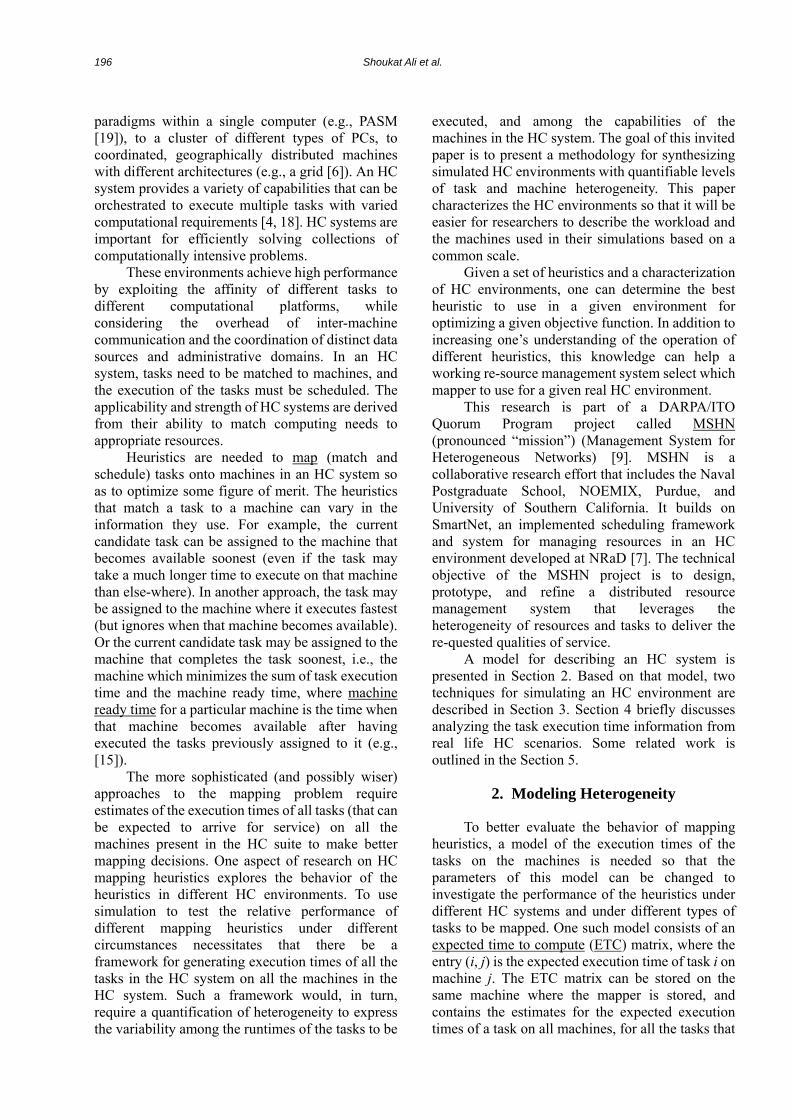
possible to obtain high task heterogeneity low machine heterogeneity ETC matrices with characteristics similar to that of low task heterogeneity high machine heterogeneity ETC matrices if Rtask = Rmach. In realistic HC systems, the variation that tasks show in their computational needs is generally larger than the variation that machines show in their capabilities. Therefore it is assumed here that requirements of high heterogeneity tasks are likely to be more “heterogeneous” than the capabilities of high heterogeneity machines (i.e., Rtask » Rmach). However, for the ETC matrices generated here, low heterogeneity in both machines and tasks is assumed to be same. Typical values for Rtask for for high and low heterogeneities are 105 and 10, respectively. And similarly for Rmach, these values are 102 and 10, respectively. Tables 1 through 4 show four ETC matrices generated by the range-based method using the above-mentioned typical values for Rtask and Rmach. The execution time values in Table 3 are much higher than the execution time values in Table 2. The difference in the values between these two tables would be reduced if the range for the low task heterogeneity was changed to 103 to 104 instead of 1 to 10.

Table 1. A low task heterogeneity low machine

heterogeneity matrix generated by the range-based method.

With the range-based method, low task heterogeneity high machine heterogeneity ETC matrices tend to have high heterogeneity for both tasks and machines, due to method used for generation. For example, in Table 2, original τ vector values were selected from 1 to 10. When each entry is multiplied by a number from 1 to 100


(1) for i from 0 to (t-1) (2) τ[i] = U ( 1, Rtask) (3) for j from 0 to (m-1) (4) e[i,j] = τ[i]× U ( 1, Rmach) (5) endfor (6) endfor

for high machine heterogeneity this generates a task heterogeneity comparable to machine heterogeneity. It is shown in Section 3.2 how to produce low task heterogeneity high machine heterogeneity ETC matrices which do show low task heterogeneity.

Figure 1. The range-based method for generating ETC matrices.

Table 2. A low task heterogeneity high machine

heterogeneity matrix generated by the range-based method.

Table 3. A high task heterogeneity low machine heterogeneity matrix generated by the range-based method.

Table 4. A high task heterogeneity high machine heterogeneity matrix generated by the range-based method.


3.2. Coefficient-of-Variation Based ETC Matrix Generation

A modification of the procedure in Figure 1 defines the coefficient of variation, V, of execution time values as a measure of heterogeneity (instead of the range of execution time values). The coefficient of variation of a set of values is a better measure of the dispersion in the values than the standard deviation because it expresses the standard deviation as a percentage of the mean of the values [13]. Let σ and µ be the standard deviation and mean, respectively, of a set of execution time values. Then V = σ / µ. The coefficient-of-variation-based ETC generation method provides a greater control over spread of the execution time values (i.e., heterogeneity) in any given row or column of the ETC matrix than the range-based method.

The coefficient-of-variation-based (CVB) ETC generation method works as follows. A task vector, q, of expected execution times with the desired task heterogeneity must be generated. Essentially, q[i] is the execution time of task i on an “average” machine in the HC suite. For example, if the HC suite consists of an IBM SP/2, an Alpha server, and a Sun SPARC 5 workstation, then q would represent estimated execution times of the tasks on the Alpha server.

To generate q, two input parameters are needed: µtask and Vtask. The input parameter, µtask is used to set the average of the values in q. The input parameter Vtask is the desired coefficient of variation of the values in q. The value of Vtask quantifies task heterogeneity, and is larger for higher task heterogeneity. Each element of the task vector q is then used to produce one row of the ETC matrix such that the desired coefficient of variation of values in each row is Vmach, another input parameter. The value of Vmach quantifies machine heterogeneity, and is larger for higher machine heterogeneity. Thus µtask, Vtask, and Vmach are the three input parameters for the CVB ETC generation method.

A direct approach to simulating HC environments should use the probability distribution that is empirically found to represent closely the distribution of task execution times. However, no standard benchmarks for HC systems are currently available. Therefore, this research uses a distribution which, though not necessarily reflective of an actual HC scenario, is flexible enough to be adapted to one. Such a distribution should not produce negative values of task execution times (e.g., ruling out Gaussian distribution), and should have a variable coefficient of variation (e.g., ruling out exponential distribution).

The gamma distribution is a good choice for the CVB ETC generation method because, with proper constraints on its characteristic parameters, it can approximate two other probability distributions, namely the Erlang-k and Gaussian (without the negative values) [13, 17]. The fact that it can approximate these two other distributions is helpful because this increases the chances that the simulated ETC matrices could be synthesized closer to some real life HC environment.

The uniform distribution can also be used but is not as flexible as the gamma distribution for two reasons: (1) it does not approximate any other distribution, and (2) the characteristic parameters of a uniform distribution cannot take all real values (explained later in the Section 3.3).

The gamma distribution [13, 17] is defined in terms of characteristic shape parameter, α, and scale parameter, β. The characteristic parameters of the gamma distribution can be fixed to generate different distributions. For example, if α is fixed to be an integer, then the gamma distribution becomes an Erlang-k distribution. If α is large enough, then the gamma distribution approaches a Gaussian distribution (but still does not return negative values for task execution times).

Figures 2(a) and 2(b) show how a gamma density function changes with the shape parameter α. When the shape parameter increases from two to eight, the shape of the distribution changes from a curve biased to the left to a more balanced bell-like curve. Figures 2(a), 2(c) and 2(d) show the effect on the distribution caused by an increase in the scale parameter from 8 to 16 to 32. The two-fold increase in the scale parameter does not change the shape of the graph (the curve is still biased to the left); however the curve now has twice as large a domain (i.e., range on x-axis).

The gamma distribution’s characteristic parameters, α and β, can be easily interpreted in terms of µtask, Vtask, and Vmach. For a gamma distribution, αβσ = , and βαµ = , so that

αµσ /1/ ==V (and 2/1 V=α ). Then αtask =

1 / Vtask2 and αmach = 1 / Vmach

2 . Further, because βαµ = , αµβ /= , and βtask = µtask / αtask. Also,

for task i, βmach [£i] = q[i] / αmach. Let G(α, β) be a number sampled from a

gamma distribution with the given parameters. (Each invocation of G(α, β) returns a new sample.) Figure 3 shows the general procedure for the CVB ETC generation.


Figure 2. Gamma probability density function for (a) α = 2, β = 8, (b) α = 8, β = 8, (c) α = 2, β = 16, and (d) α = 2, β = 32.

(1) αtask = 1 / Vtask2 ; αmach = 1 / Vmach

2 ; βtask = µtask / αtask

(2) for i from 0 to (t – 1) (3) q[i] = G( αtask ,βtask ) /* q[i] will be used as mean of i-th row of ETC matrix */ (4) βmach [i] = q[i] / αmach /* scale parameter for i-th row */ (5) for j from 0 to (m – 1) (6) e[i,j] = G( αmach, βmach[i]) (7) endfor (8) endfor

Figure 3. The general CVB method for generating ETC matrices.

Given the three input parameters, Vtask , Vmach,

and µtask, Line (1) of Figure 3 determines the shape parameter αtask and scale parameter βtask of the gamma distribution that will be later sampled to build the task vector q. Line (1) also calculates the shape parameter αmach to use later in Line (6). In the i-th iteration of the outer for loop (Line 2) in Figure 3, a gamma distribution with parameters αtask and βtask is sampled to obtain q[i]. Then q[i] is used to determine the scale parameter βmach[i] (to be used later in Line (6)). For the i-th iteration of the outer for loop (Line 2), each iteration of the inner for loop (Line 5) produces one element of the i-th row of the ETC matrix by sampling a gamma distribution with parameters αmach and βmach [i]. One complete row of the ETC matrix is produced by m iterations of the inner for loop (Line 5). Note that while each row in


the ETC matrix has gamma distributed execution times, the execution times in columns are not gamma distributed.

The ETC generation method of Figure 3 can be used to generate high task heterogeneity high machine heterogeneity ETC matrices, high task heterogeneity low machine heterogeneity ETC matrices, and low task heterogeneity low machine heterogeneity ETC matrices, but cannot generate low task heterogeneity high machine heterogeneity ETC matrices. To satisfy the heterogeneity quadrants of Section 2, each column in the final low task heterogeneity high machine heterogeneity ETC matrix should reflect the low task heterogeneity of the “parent” task vector q. This condition would not necessarily hold if rows of the ETC matrix were produced with a high machine heterogeneity from a task vector of low heterogeneity. This is because a given column may be formed from widely different execution time values from different rows because of the high machine heterogeneity. That is, any two entries in a given column are based on different values of q[i] and αmach, and may therefore show high task heterogeneity as opposed to the intended low task heterogeneity. In contrast, in a high task heterogeneity low machine heterogeneity ETC matrix the low heterogeneity among the machines for a given task (across a row) is based on the same q[i] value.

One solution is to generate what is in effect a transpose of a high task heterogeneity low machine heterogeneity matrix to produce a low task heterogeneity high machine heterogeneity one. The transposition can be built into the procedure as shown in Figure 4.

The procedure in Figure 4 is very similar to the one in Figure 3. The input parameter µtask is

replaced with µmach. Here, first a machine vector, p, (with an average value of µmach) is produced. Each element of this “parent” machine vector is then used to generate one low task heterogeneity column of the ETC matrix, such that the high machine heterogeneity present in p is reflected in all rows. This approach for generating low task heterogeneity high machine heterogeneity ETC matrices can also be used with the range-based method.

(1) αtask = 1 / Vtask

2 ; αmach = 1 / Vmach2 ;

βmach = µmach / αmach (2) for j from 0 to (m – 1) (3) p[j] = G( αmach ,βmach ) /* p[j] will be used as mean of j-th column of ETC matrix */ (4) βtask [j] = p[j] / αtask /* scale parameter for j-th column */ (5) for i from 0 to (t – 1) (6) e[i,j] = G( αtask, βtask[j]) (7) endfor (8) endfor

Figure 4. The CVB method for generating low task

heterogeneity high machine heterogeneity ETC matrices.

Tables 5 through 10 show some sample ETC

matrices generated using the CVB ETC generation method. Tables 5 and 6 both show high task heterogeneity low machine heterogeneity ETC matrices. In both tables, the spread of the execution time values in columns is higher than that in rows. The ETC matrix in Table 6 has a higher task heterogeneity (higher Vtask) than the ETC matrix in Table 5. This can be seen in a higher spread in the columns of matrix in Table 6 than that in Table 5.

Table 5. A high task heterogeneity low machine heterogeneity matrix generated by the CVB

method. Vtask = 0.3 , Vmach = 0.1.


Table 6. A high task heterogeneity low machine heterogeneity matrix generated by the CVB method. Vtask = 0.5 , Vmach = 0.1.

Table 7. A high task heterogeneity high machine heterogeneity matrix generated by the CVB


Table 8. A low task heterogeneity low machine heterogeneity matrix generated by the CVB



Table 9. A low task heterogeneity high machine heterogeneity matrix generated by the CVB method. Vtask = 0.1 , Vmach = 0.6.

Table 10. A low task heterogeneity high machine heterogeneity matrix generated by

the CVB method. Vtask = 0.1 , Vmach = 2.0.

Tables 7 and 8 show high task heterogeneity high machine heterogeneity and low task heterogeneity low machine heterogeneity ETC matrices, respectively. The execution times in Table 7 are widely spaced along both rows and columns. The spread of execution times in Table 8 is smaller along both columns and rows, because both Vtask and Vmach are smaller.

Tables 9 and 10 show low task heterogeneity

high machine heterogeneity ETC matrices. In both tables, the spread of the execution time values in rows is higher than that in columns. ETC matrix in Table 10 has a higher machine heterogeneity (higher Vmach) than the ETC matrix in Table 9. This can be seen in a higher spread in the rows of matrix in Table 10 than that in Table 9.

3.3. Uniform Distribution in the CVB Method

The uniform distribution could also be used for the CVB ETC generation method. The uniform distribution’s characteristic parameters a (lower bound for the range of values) and b (upper bound for the range of values), can be easily interpreted in terms of µtask, Vtask, and Vmach. (Recall that Vtask = σtask/µtask and Vmach = σmach / µmach). For a uniform distribution, 12/)( ab −=σ and 2/)( ab +=µ [17]. So that

µ2=+ ba (1)

12σ−=− ba (2)


Adding Equations (1) and (2),

3σµ −=a (3)

)3)/(1( µσµ −=a (4)

)31( Va −= µ (5) Also,

ab −= µ2 (6) The Equations (5) and (6) can be used to generate the task vector q from the uniform distribution with the following parameters:

)31( tasktasktask Va −= µ (7)

tasktasktask ab −= µ2 (8) Once the task vector q has been generated, the i-the row of the ETC matrix can be generated by sampling (m times) a uniform distribution with the following parameters:

)31]([ machmach Viqa −= (9)

machmach aiqb −= ][2 (10)

The CVB ETC generation using the uniform distribution, however, places a restriction on the values of Vtask and Vmach. Because both atask and amach have to be positive, it follows from Equations (7) and (9) that the maximum value for Vmach or Vtask is

3/1 . Thus, for the CVB ETC generation, the gamma distribution is better than the uniform distribution because it does not restrict the values of task or machine heterogeneities.

3.4. Producing Consistent ETC Matrices

The procedures given in Figures 1, 3, and 4 produce inconsistent ETC matrices. Consistent ETC matrices can be obtained from the inconsistent ETC matrices generated above by sorting the execution times for each task on all machines (i.e., sorting the values within each row and doing this for all rows independently). From the inconsistent ETC matrices generated above, partially-consistent matrices consisting of an i × k sub-matrix could be generated by sorting the execution times across a random

subset of k machines for each task in a random subset of i tasks.

It should be noted from Tables 9 and 10 that the greater the difference in machine and task heterogeneities, the higher the degree of consistency in the inconsistent low task heterogeneity high machine heterogeneity ETC matrices. For example, in Table 10 all tasks show consistent execution times on all machines except on the machines that correspond to columns 3 and 4. As mentioned in Section 1, these degrees and classes of mixed-machine heterogeneity can be used to characterize many different HC environments.

4. Analysis and Synthesis

Once the actual ETC matrices from a real life scenario are obtained, they can be analyzed to estimate the probability distribution of the execution times, and the values of the model parameters (i.e., Vtask, Vmach, and µtask (or µmach, if a low task heterogeneity high machine heterogeneity ETC matrix is desired)) appropriate for the given real life scenario. The above analysis could be carried out using common statistical procedures [11]. Once a model of a particular HC system is available, the effect of changes in the workload (i.e., the tasks arriving for service in the system) and the system (i.e., the machines present in the HC system) can be studied in a controlled manner by simply changing the parameters of the ETC model.

This experimental setup can then be used to find out which mapping heuristics are best suited for a given set of model parameters (i.e., Vtask, Vmach, and µtask (or µmach)). This information can be stored in a “look-up table,” so as to facilitate the choice of a mapping heuristic given a set of model parameters. The look-up table can be part of the toolbox in the mapper.

The ETC model of Section 2 assumes that the machine heterogeneity is the same for all tasks, i.e., different tasks show the same general variation in their execution times over different machines. In reality this may not be true; the variation in the execution times of one task on all machines may be very different from some other task. To model the “variation in machine heterogeneity” along different rows (i.e., for different tasks), another level of heterogeneity could be introduced. For example, in the CVB ETC generation, instead of having a fixed value for Vmach for all the tasks, the value of Vmach for a given task could be variable, e.g., it could be sampled from a probability distribution. Once again, the nature of the probability distribution and its parameters will need to be decided empirically.


5. Related Work

To the best of the authors’ knowledge, there is currently no work presented in the open literature that addresses the problem of modeling of execution times of the tasks in an HC system (except the already discussed work [15]). However, below are presented two tangentially related works.

A detailed workload model for parallel machines has been given in [5]. However the model is not intended for HC systems in that the machine heterogeneity is not modeled. Task execution times are modeled but tasks are assumed to be running on multiple processing nodes, unlike the HC environment presented here where tasks run on single machines only.

A method for generating random task graphs is given in [21] as part of description of the simulation environment for the HC systems. The method proposed in [21] assumes that the computation cost of a task ti, averaged over all the machines in the system, is available as iw . The method does provide for characterizing the differences in the execution times of a given task on different processors in the HC system (i.e., machine heterogeneity). The “range percentage” (ß) of computation costs on processors roughly corresponds to the notion of machine heterogeneity as presented here. The execution time, ei j , of task ti on machine mj is randomly selected from the range,

)2/1()2/1( ββ +×≤≤−× iiji wew . However, the method in [21] does not provide for describing the differences in the execution times of all the tasks on an “average” machine in the HC system. The method in [21] does not tell how the differences in the values of iw for different tasks will be modeled. That is, the method is [21] does not consider task heterogeneity. Further, the model in [21] does not take into account the consistency of the task execution times.

6. Conclusions

To describe different kinds of heterogeneous environments, an existing model based on the characteristics of the ETC matrix was presented. The three parameters of this model (task heterogeneity, machine heterogeneity, and consistency) can be changed to investigate the performance of mapping heuristics for different HC systems and different sets of tasks. An existing range-based method for quantifying heterogeneity was described, and a new coefficient-of-variation-

based method was proposed. Corresponding procedures for generating the ETC matrices representing various heterogeneous environments were presented. Sample ETC matrices were provided for both ETC generation procedures. The coefficient-of-variation-based ETC generation method provides a greater control over the spread of values (i.e., heterogeneity) in any given row or column of the ETC matrix than the range-based method. This characterization of HC environments will allow a researcher to simulate different HC environments, and then evaluate the behavior of the mapping heuristics under different conditions of heterogeneity.

Acknowledgment

The authors thank Anthony A. Maciejewski, Tracy D. Braun, and Taylor Kidd for their valuable comments and suggestions. A preliminary version of portions of this material was presented at the 9th Heterogeneous Computing Workshop, sponsored by the IEEE Computer Society and the US Office of Naval Research.

References

[1] Armstrong, R., “Investigation of Effect of Different Run-Time Distributions on Smart-Net Performance,” Master’s thesis, Naval Postgraduate School (1997) (D. Hensgen, Advisor).

[2] Braun, T. D., Siegel, H. J., Beck, N., Bölöni, L., Maheswaran, M., Reuther, A. I., Robertson, J. P., Theys, M. D., Yao, B., Freund, R. F., and Hensgen, D., “A Comparison Study of Static Mapping Heuristics for a Class of Meta-Tasks on Heterogeneous Computing Systems,” 8th IEEE Heterogeneous Computing Workshop (HCW ’99), pp. 15–29 (1999).

[3] Dietz, H. G., Cohen, W. E., and Grant, B. K., “Would You Run It Here... Or There? (AHS: Automatic Heterogeneous Supercomputing),” 1993 International Conference on Parallel Processing (ICPP ’93), Vol. II, pp. 217–221 (1993).

[4] Eshaghian, M. M., ed., Heterogeneous Computing, Artech House, Norwood, MA (1996).

[5] Feitelson, D. G. and Rudolph, L., “Metrics and Benchmarking for Parallel Job Scheduling,” in D. G. Feitelson, L. Rudolph, eds., Job Scheduling Strategies for Parallel Processing, Lecture Notes in Computer Science, Springer-Verlag, New York, NY, Vol. 1459, pp. 1–15 (1998).


[6] Foster, I., Kesselman, C., eds., The Grid: Blueprint for a New Computing Infrastructure, Morgan Kaufmann, San Fransisco, CA (1999).

[7] Freund, R. F., Gherrity, M., Ambrosius, S., Campbell, M., Halderman, M., Hensgen, D., Keith, E., Kidd, T., Kussow, M., Lima, J. D., Mirabile, F., Moore, L., Rust, B., and Siegel, H. J., “Scheduling Resources in Multi-User, Heterogeneous, Computing Environments with SmartNet,” 7th IEEE Heterogeneous Computing Workshop (HCW ’98), pp. 184–199 (1998).

[8] Ghafoor, A. and Yang, J., “Distributed Heterogeneous Supercomputing Management System,” IEEE Computer, Vol. 26, No. 6, pp. 78– 86 (1993).

[9] Hensgen, D. A., Kidd, T., John, D. S., Schnaidt, M. C., Siegel, H. J., Braun, T. D., Maheswaran, M., Ali, S., Kim, J.-K., Irvine, C., Levin, T., Freund, R. F., Kussow, M., Godfrey, M., Duman, A., Carff, P., Kidd, S., Prasanna, V., Bhat, P., and Alhusaini, A., “An Overview of MSHN: The Management System for Heterogeneous Networks,” 8th IEEE Heterogeneous Computing Workshop (HCW ’99), pp. 184–198 (1999).

[10] Iverson, M. A., Özgüner, F., and Follen, G. J., “Statistical Prediction of Task Execution Times Through Analytic Benchmarking for Scheduling in a Heterogeneous Environment,” 8th IEEE Heterogeneous Computing Workshop (HCW ’99), pp. 99–111 (1999).

[11] Jain, R., The Art of Computer Systems Performance Analysis, John Wiley & Sons, Inc., New York, NY (1991).

[12] Kafil, M. and Ahmad, I., “Optimal Task Assignment in Heterogeneous Distributed Com-putting Systems,” IEEE Concurrency, Vol. 6, No. 3, pp. 42–51 (1998).

[13] Lapin, L. L., Probability and Statistics for Modern Engineering, Waveland Press, Inc., Prospect Heights, IL, Second edn. (1998).

[14] Lopez-Benitez, N. and Hyon, J.-Y., “Simulation of Task Graph Systems in Heterogeneous Computing Environments,” 8th IEEE Heterogeneous Computing Workshop (HCW ’99), pp. 112–124 (1999).

[15] Maheswaran, M., Ali, S., Siegel, H. J., Hensgen, D., and Freund, R. F., “Dynamic Mapping of a Class of Independent Tasks onto Heterogeneous Computing Systems,” Journal of Parallel and Distributed Computing, Vol. 59, No. 2, pp. 107–131 (1999).

[16] Maheswaran, M., Braun, T. D., and Siegel, H. J., “Heterogeneous Distributed Computing,” in

J. G. Webster, ed., Encyclopedia of Electrical and Electronics Engineering, Vol. 8, John Wiley, New York, NY, pp. 679–690 (1999).

[17] Papoulis, A., Probability, Random Variables, and Stochastic Processes, McGraw-Hill, New York, NY (1984).

[18] Siegel, H. J. and Ali, S., “Techniques for Mapping Tasks to Machines in Heterogeneous Computing Systems,” Journal of Systems Architecture, Vol. 46, No. 8, pp. 627–639 (2000).

[19] Siegel, H. J., Braun, T. D., Dietz, H. G., Kulaczewski, M. B., Maheswaran, M., Pero, P. H., Siegel, J. M., So, J. J. E., Tan, M., Theys, M. D., and Wang, L., “The PASM Project: A Study of Reconfigurable Parallel Computing,” 2nd International Symposium on Parallel Architectures, Algorithms, and Networks (ISPAN’96), pp. 529–536 (Invited paper) (1996).

[20] Singh, H. and Youssef, A., “Mapping and Scheduling Heterogeneous Task Graphs Using Genetic Algorithms,” 5th IEEE Heterogeneous Computing Workshop (HCW ’96), pp. 86–97 (1996).

[21] Topcuoglu, H., Hariri, S., and Wu, M.-Y., “Task Scheduling Algorithms for Heterogeneous Processors,” 8th IEEE Heterogeneous Computing Workshop (HCW ’99), pp. 3–14 (1999).

[22] Yang, J., Ahmad, I. and Ghafoor, A., “Estimation of Execution Times on Heterogeneous Supercomputer Architecture,” 1993 International Conference on Parallel Processing (ICPP ’93), Vol. I, pp. 219–225 (1993).

Representing Task and Machine Heterogeneities for Heterogeneous Computing Systems

Documents

Transcript of Representing Task and Machine Heterogeneities for Heterogeneous Computing Systems