Representative point-integrated suspended

sediment sampling in rivers

by

Alessandro B. Gitto

B.Sc., University of Western Ontario, 2012

Thesis Submitted in Partial Fulfillment of the

Requirements for the Degree of

Master of Science

in the

Department of Geography

Faculty of Environment

Alessandro B. Gitto 2015

SIMON FRASER UNIVERSITY

Fall 2015

ii

Approval

Name: Alessandro B. Gitto

Degree: Master of Science (Geography)

Title: Representative point-integrated suspended sediment sampling in rivers

Examining Committee: Chair: Nadine Schuurman Professor

Jeremy Venditti Senior Supervisor Associate Professor

Michael Church Supervisor Professor Emeritus Department of Geography University of British Columbia

Ray Kostaschuk Supervisor Adjunct Professor

Brian Menounos External Examiner Professor Department of Geography University of Northern British Columbia

Date Defended/Approved:

September 29, 2015

iii

Abstract

Point-integrated bottle sampling is the traditional method to determine the mean

concentration of suspended sediment. Sample duration is assumed to average over

enough variability to represent the mean suspended sediment concentration. Inadequate

time averaging in relation to point-integrated sampling remains unexamined. Here, we

analyze continuous hour-long measurements of suspended sediment and grain size

fractions collected using a LISST-SL in the sand bedded portion of the Fraser River, BC.

Mean concentrations for suspended sediment and grain size fractions were computed

over increasing time periods and compared to a long duration mean concentration to

determine when a sample became representative. A cumulative probability distribution

was generated for multiple iterations of this process. All suspended sediment load and

grain size fractions bear a low probability of accurately representing the actual mean

concentration over standard bottle sample durations. A probability >90% of accurately

representing the mean of volumetric concentration requires 9.5 minutes of sampling.

Keywords: suspended sediment; point-integrated bottle sampling; LISST-SL

iv

Acknowledgements

I would like to thank my supervisory committee, Jeremy Venditti, Michael Church, and

Ray Kostaschuk, for their guidance and feedback throughout this process. I would

especially like to thank Jeremy and Mike for teaching me everything I know about fluvial

geomorphology. Thank you also to my examining committee, Brian Menounos and

Kirsten Zickfield for their additional insights and comments to improve my thesis.

I would like to thank Ray and Jeremy for their help during my fieldwork. I would also like

to acknowledge funding from NSERC Discovery grants (Jeremy Venditti).

Special thank you to Ryan Bradley who has been a great friend and mentor and thanks

to Dan Haught who taught me beer and MATLAB. Thank you to Krystyna Adams for her

love and support and thank you to my family who has always been so encouraging.

v

Table of Contents

Approval .............................................................................................................................ii Abstract ............................................................................................................................. iii Acknowledgements ...........................................................................................................iv Table of Contents .............................................................................................................. v List of Tables .................................................................................................................... vii List of Figures.................................................................................................................. viii

1.0. Introduction ......................................................................................................... 1

2.0. Methods ................................................................................................................ 5 2.1. Study Site ................................................................................................................. 5 2.2. Observations ............................................................................................................ 6 2.3. Data Analysis ........................................................................................................... 7

3.0. Results ............................................................................................................... 13 3.1. Variability in grain size and concentration .............................................................. 13 3.2. Spectral Estimates ................................................................................................. 15 3.3. Cumulative probability of NSMV method ................................................................ 19 3.4. Temporary stabilization of ................................................................................... 21

3.4.1. Suspended sediment loads ....................................................................... 21 3.4.2. Grain size fractions ................................................................................... 24

4.0. Discussion ......................................................................................................... 30

5.0. Conclusion ......................................................................................................... 33

References .................................................................................................................. 34 Appendix A. Power spectral estimates of suspended sediment load ............................. 38

Volumetric Concentration ....................................................................................... 38 Silt load .................................................................................................................. 39 Washload ............................................................................................................... 41 Suspended bed material ........................................................................................ 42 D50 .................................................................................................................. 43

Appendix B. Persistent stabilization of ........................................................................ 44 Suspended sediment loads .................................................................................... 45 Grain size fractions................................................................................................. 46

Appendix C. Sampling time for a specified level of probability ....................................... 47 Suspended sediment loads .................................................................................... 47 Grain size fractions................................................................................................. 49

vi

Appendix D. Point of diminishing returns ....................................................................... 51 Suspended sediment loads .................................................................................... 52 Grain size fractions................................................................................................. 52

vii

List of Tables

Table 3.1. Summary of the dominant periods underlying the downstream water velocity spectral signal. All values in the table are presented in seconds. .............................................................................................. 18

Table 3.2. Time in seconds to achieve a specified level of probability of representing mean suspended sediment load concentration using temporary stabilization. Times were recorded from the cumulative probability curves of Sites 1 and 2. Each variable is depth averaged for the associated probability level. ......................................... 26

Table 3.3. Time in seconds to achieve a specified level of probability of representing grain size fraction using temporary stabilization. Times were recorded from the cumulative probability curves of Sites 1 and 2. Each variable is depth averaged for the associated probability level. ....................................................................................... 28

viii

List of Figures

Figure 2.1. Grain size distribution captured by the LISST-SL a) before and b) after erroneous first 4 and last 2 bins were removed. Instantaneous concentrations for each grain size bin over a ten-minute period are presented. ..................................................................... 8

Figure 2.2. Example of non-stationary mean value for sand load at 0.6h of Site 2. The confidence bounds represent a range of mean values characteristic of the true mean value for a given sample size. As

the incremental mean value , increases in sample size it may become representative for a minimum of 60 seconds and be

considered to stabilize temporarily. will also become representative for the duration of the measurement and may be considered to stabilize persistently. ......................................................... 12

Figure 3.1. Representative time series at Site 2, 0.6h of a) volumetric concentration, silt load, washload, sand load, and suspended bed material and b) D10, D16, D50, D84, and D90. .............................................. 14

Figure 3.2. Coefficient of variation for a) Sites 1 and b) 2 computed for each LISST-SL grain size bin. .......................................................................... 15

Figure 3.3. Spectral estimates of streamwise velocity from Sites 1 and 2 for 0.1h, 0.2h, 0.4h, 0.6h, 0.8h, and 0.9h. ..................................................... 16

Figure 3.4. Examples of spectral estimates of suspended sediment concentration for various fractions at 0.6h of Site 2. ............................... 17

Figure 3.5. Comparison between cumulative probability plots on the condition of (a) persistent stabilization and (b) temporary stabilization from 0.1h of Site 2. Results from (b) show a higher probability of a short duration sample approximating the long-term average than is observed in (a). ........................................................................................ 20

Figure 3.6. Cumulative probability plots of suspended sediment loads with the

condition of temporary stabilization of the signal. Measurements from Site 1 at a) 0.1h, b) 0.2h, c) 0.4h, d) 0.8h, and Site 2 at e) 0.1h, f) 0.2h, g) 0.4h, and h) 0.6h show the cumulative probability of obtaining a sample with a representative grain size moment value when measuring for a given period of time. ................................... 23

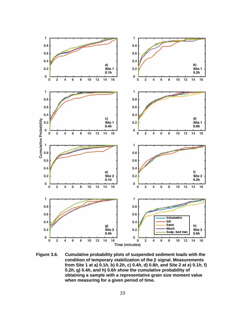
Figure 3.7. Cumulative probability plots of grain size fractions with the

condition of temporary stabilization of the signal. Measurements from Site 1 at a) 0.1h, b) 0.2h, c) 0.4h, d) 0.8h, and Site 2 at e) 0.1h, f) 0.2h, g) 0.4h, and h) 0.6h show the cumulative probability of obtaining a sample with a representative grain size moment value when measuring for a given period of time. ................................... 25

1

1.0. Introduction

Fluvial sediment transport is a key component of the overall denudation of the

continental surface [Milliman and Meade, 1983; Milliman and Syvitski, 1992]. Sediment

in rivers may be transported either in suspension, as bedload, or in solution. The

suspended load is comprised of materials supported by upward fluid stress sufficient to

keep a particle from settling to the bed. The finest portion of the suspended load is the

washload, which typically constitutes less than 10% of the bed material and is

transported in near-continuous suspension [Church, 2006]. Bed material is coarser than

washload but may also travel in suspension provided the upward directed fluid stresses

are greater than the downward settling velocity of the sediment grains [Bridge, 2003].

Bedload comprises the coarsest particles, which move by rolling, sliding, or saltating

along the bed. Globally, suspended sediment contributions to the oceans account for an

estimated 16.2 x 109 tons annually while bedload is about 1.6 x 109 tons [Syvitski et al.,

2005].

Suspended sediment concentrations are typically measured by collecting

samples of water-sediment mixtures. Bottle samples are the traditional method for

obtaining suspended sediment samples and may be collected using either depth- or

point-integrated methods. Depth-integrated sampling involves lowering the sediment

sampler from the river surface to the bed of the channel at a uniform rate while a bottle

within the sampler collects an incremental volume of the water-sediment mixture from all

points along the sampled depth. Each location chosen for a measurement is known as a

sampling vertical and the movement of the sampler from the surface to the bed, or vice

versa, is known as a transit. Point-integrated sampling involves lowering the sampler to

a specific depth in the water column and collecting a volume of water-sediment mixture

at a particular point in the flow [Tassone and Lapointe, 1999]. The number of point-

integrated samples recommended for a channel >5m depth is 7: one measurement is

made at the surface, another at the bed, and five more at 0.2h, 0.4h, 0.6h, 0.8h, and

2

0.9h where h is channel depth [Tassone and Lapointe, 1999]. This type of bottle

sampling is designed to capture the mean suspended sediment concentration in the flow

through time averaging.

Topping et al. [2011] identified four common sources of error arising from depth-

integrated suspended sediment sampling: (1) bed contamination, (2) pressure-driven

inrush, (3) inadequate number of sampling verticals collected across the channel width,

and (4) inadequate time averaging. Error arising from (1) and (2) is the result of improper

use of the suspended sediment sampler and can be easily rectified. Additional verticals

across the channel will reduce uncertainty associated with (3) [Topping et al., 2011]. To

address the uncertainty with inadequate time averaging Topping et al. [2011]

recommended doubling the number of transits in standard two-way depth integrated

sampling, which introduces minimal time averaging at all points of the depth. This

method was found to reduce uncertainty by ~30% in each grain size class between

multiple samples.

The error associated with point-integrated suspended sediment bottle sampling

has not been addressed in the literature. It is reasonable to assume that point-

integrated sampling is subject to the same user-induced errors, inadequate cross-

section sampling and inadequate time averaging problems identified by Topping et al.

[2011]. These sources of error can also be resolved in the same way, but it is not clear

how many additional point-integrated samples need to be taken to obtain an accurate

estimate of suspended sediment concentration. Indeed, the time required to obtain an

accurate estimate of suspended sediment concentration in rivers is not known because

the minimum time for a sample is set by the need to adequately average over variability

in the flow. The maximum duration of bottle sampling is constrained by the volume of the

bottle and flow velocity. If point-integrated sampling techniques are designed to

represent the mean concentration in suspension [Tassone and Lapointe, 1999] then the

sample duration of the bottle sampler must average enough variability in the flow to

provide an accurate estimate of the mean. The accuracy of the sample relates to the

closeness of the suspended sediment sample to the true underlying mean value. The

true underlying mean value is affected by intermediate frequency variability in flow and

sediment concentration on the order of minutes to possibly tens of minutes in duration.

3

The precision of the sample relates to the how closely multiple measurements of the

mean concentration resemble each other. The precision of the sample is affected by

high frequency variation in the suspended sediment concentration occurring over

seconds to minutes. Repeated samples of suspended sediment are required to improve

the accuracy of the measurements and to identify the appropriate sample period that will

account for both intermediate and high frequency fluctuations in suspended sediment

and fluid flow variability.

Variability in suspended sediment concentration is associated with variations in

fluid velocity. Fluctuations in the downstream or cross-stream fluid velocity are the result

of fluid flow events varying in magnitude and frequency. At the finest scales, variability in

fluid flow is induced by turbulent fluctuations; at the largest scales, variability exists in

climatic contributions to annual flow conditions. Between these two extremes of the fluid

velocity spectrum exist coherent flow structures (CFS), which occupy all scales of

turbulent fluid flow and contribute energy and momentum mixing to the transport of

material in the flow. Low magnitude, high frequency near-wall CFS such as low-speed

streaks [Kline et al, 1967], sweeps and ejections [Lapointe, 1992], and quasi-streamwise

vortices [Adrian, 2013] occur in the near-wall portion of the inner layer [Adrian and

Marusic, 2012]. Large-scale motions (LSM) of intermediate frequency such as kolks

[Kostaschuk and Church, 1993] are upward sweeping fluid vortices that are also

effective at entraining bed sediment into suspension. Large CFS features such as very

large-scale motions (VLSM) occupy the entire water column and extend roughly 20

times the boundary layer thickness downstream [Hutchins and Marusic, 2007]. It

remains unclear whether VLSM are discrete, random CFS features or if they are an

amalgamation of LSM aligned in the streamwise direction [Adrian and Marusic, 2012;

Marquis and Roy, 2013]. It is also unclear if VLSM actively erode and transport sediment

or if the composite smaller motions perform this task [Adrian and Marusic, 2012].

Fluctuation in suspended sediment concentrations is related to availability of

sediment and the incidence of shear stresses capable of entrainment. Higher

concentrations of suspended sediment are strongly correlated with higher upward

velocities capable of vertical mixing [Lapointe, 1992, 1996; Kostaschuk and Church

1993; Shugar et al., 2010; Bradley et al., 2013; Kwoll et al., 2014]. At the finest scales,

4

sweeps and ejections are brief events, lasting 3-8 seconds, which contribute the bulk

majority of vertical sediment mixing [Lapointe, 1992]. In tidal rivers, contributions to net

sediment flux over tidal cycles are dominant during low tide when mean flow velocities

are highest [Kostaschuk and Best, 2005; Bradley et al., 2013; Kwoll et al., 2014].

Observations also indicate that, under decelerating flows resulting from rising tides,

enhanced turbulence produces larger scale suspension events [Kostaschuk and Best,

2005], although the contribution to net sediment flux does not appear to be as great

[Bradley et al., 2013; Kwoll et al., 2014].

The interaction of all sources of variability produces varying suspended sediment

concentrations. Improving suspended sediment sampling techniques relies on

understanding the contributing sources of variability and the frequency and magnitude

with which they occur. By identifying the frequency of the dominant events influencing

suspended sediment concentrations, the maximum time period over which the flow

should be sampled can be established. An ideal record length balances the need to

adequately capture high-frequency contributions to the downstream flow variability

generated by interaction of the flow with the boundary without capturing externally forced

low-frequency changes in flow lasting hours or longer (nival events, synoptic scale

floods, tidal influences [e.g. Soulsby, 1980]). Here, we seek to establish the time

required to collect a point-integrated sample of suspended sediment with a

representative mean concentration. A representative mean concentration is the

concentration of suspended sediment in flux after turbulence in the signal has been

averaged out. Do current point-sample measurement techniques adequately capture

mean concentration of suspended sediment? What sample duration is required to obtain

an accurate mean concentration? Does the time required to obtain a representative

mean concentration vary for different components of the suspended sediment load?

5

2.0. Methods

2.1. Study Site

Field measurements were conducted along a reach of the Fraser River at

Mission, British Columbia, Canada, approximately 85 km upstream of the outlet of the

river where it flows into the Strait of Georgia. Mission is 15 km downstream of the gravel-

sand transition in the Fraser River, which is associated with a substantial break in water

surface slope that delivers suspended sand to the bed [Venditti and Church, 2014]. The

bed material at Mission is 0.38 mm sand forming small dune features over most of the

bed during moderate to high flows.

Mean annual flow at Mission is 3410 m3 s-1 and the mean annual flood is 9790

m3 s-1 [McLean et al., 1999]. Major discharge events are dominated by the spring

snowmelt beginning in April with peak discharges between May and July before

discharge recedes through August and September [Venditti et al., 2014]. The Mission

reach of the Fraser River experiences minor tidal effects during the freshet but no

saltwater intrusion (see Dashtgard et al., 2012 for a recent review). This reach also has

minimal boat traffic, allowing for long instrument deployments, and there has been a

considerable number of previous works characterizing sediment transport in the reach

[McLean et al., 1999; Domarad, 2011; Attard, 2012; Attard et al., 2014; Venditti and

Church, 2014; Venditti et al., 2015].

Peaks in sediment transport precede annual peaks in flow discharge during

freshets. On the basis of a sediment transport measurement program undertaken by the

Water Survey of Canada between 1966 and 1986, McLean et al. [1999] reported the

mean total suspended load is 17 x106 t yr-1 of which, suspended clay (<1 m) accounts

for 2.3 x106 t yr-1, silt load (<64 m) is 8.3 x106 t yr-1, and sand load (>64 m) is 6.1 x106 t

yr-1. The nominal division between washload and bed material load at Mission is 0.18

6

mm [McLean et al., 1999; Attard et al., 2014]. The washload comprises the vast majority

of the total suspended load, accounting for 14 x106 t yr-1. The remaining 18% of total

suspended load is the suspended bed-material load. The annual bedload is estimated to

be 1.5 x105 t yr-1 [McLean et al., 1999].

2.2. Observations

Continuous records of suspended sediment concentration were collected from

May 30 to June 2, 2013 using a Sequoia LISST-SL (laser in-situ scattering

transmissometer), a streamlined instrument with stabilizing fins that uses laser diffraction

to sample instantaneous volumetric particle concentration, grain-size distribution,

downstream water velocity, optical transmission, depth, and water temperature

information at 0.5 Hz [Sequoia Scientific, 2012]. Data were recorded in 32 log-spaced

bins ranging from 1.90 to 381 m. The instrument isokinetically pumps water through a

front nozzle and into a laser detection chamber. The pump is dynamically adjusted to

match water velocity at the instrument nose measured using a pitot tube. Data were

recorded in a topside control box for post-processing. No physical samples of

suspended sediment were collected. We made no attempt to compare the LISST-SL

concentrations and grain-size to conventional bottle samples because we are interested

in the variability of the signal and not the absolute values of any variable.

Suspended sediment concentration data were measured from a 6 m boat.

Average discharge over this period was 8265 m3 s-1, just below the mean annual peak

flow. The LISST-SL was deployed from the side of the boat with a USGS B-reel

operated through a davit to allow measurement at desired depths. Slight modifications to

the Water Survey of Canada’s sampling program were made to ensure optimal use of

the sediment sampler. Instead of a measurement collected at the surface, a

measurement was made at 0.1h to ensure the sampler remained submerged for the

entire duration. Samples were not collected close to the bed to avoid potential

instrument clogging with coarse sediment and contact with the bed. As a result 6 points

in the water column were measured, each for 1 hour: 0.1h, 0.2h, 0.4h, 0.6h, 0.8h, and

0.9h. Vertical position was measured with an onboard pressure sensor. Spatial

coordinates were recorded using differential GPS. Two locations were selected near

7

Mission, B.C; Site 1 is located at 4907’39” N, 12217’50” W and Site 2 is located 0.2 km

upstream at 4907’42” N, 12217’41” W. The bed at both locations is approximately flat

with small dune features rising on average 10 cm from the bed. Bed material samples

were collected at both locations by dredging a portion of the bed with a grab sampler.

2.3. Data Analysis

Data from the LISST-SL topside control box were processed using MATLAB

code that employed Sequoia’s irregular shaped particle model to calculate total

volumetric, silt (<64 m), sand (>64 m), washload (<177 m) and suspended bed

material (>177 µm) concentrations as well as grain size fractions. Inspection of the

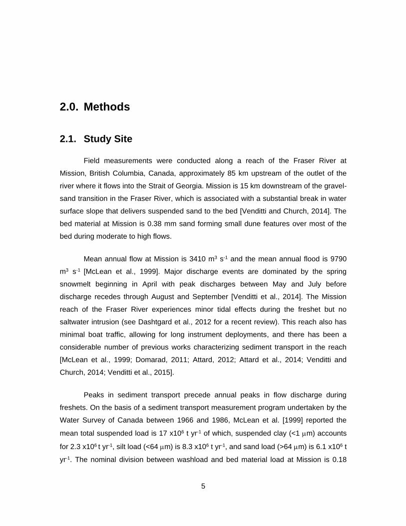
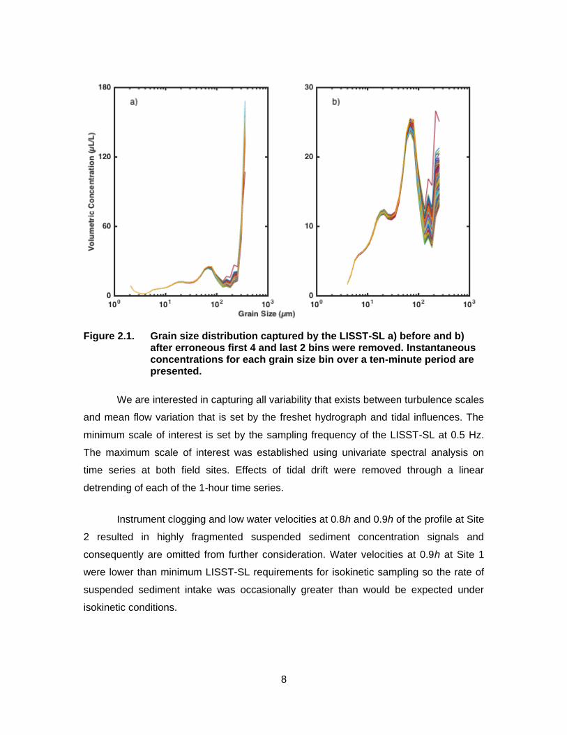
empirically derived frequency curves of the collected data indicated a spike in

concentration in the first four and last two grain-size bin classes measured by the LISST-

SL. Grain sizes between 1.90 – 3.69 m and 273 – 381 µm are at the edge of the laser

detector and are most susceptible to errors if the laser alignment is not perfect (See

Domarad, 2011). These grain-size bins were removed from subsequent analysis so that

the measured range of suspended sediment is 3.69-273 µm (Figure 2.1). To determine

the effect of this truncation, a comparison of the grain size distribution to a cumulative

distribution of suspended sediment collected during freshet at Mission in 1974 and an

image analysis of physical samples of suspended sediment collected in 2015 was

performed. The comparison indicates ~15% of the coarsest portion of the grain size

distribution is not measured with the 273 µm cut off. Additionally we explored the

variability in volumetric concentration in each grain-size bin by calculating the coefficient

of variation, which is the standardized measure of dispersion of a probability distribution,

defined as the ratio of the standard deviation , to the mean .

8

Figure 2.1. Grain size distribution captured by the LISST-SL a) before and b) after erroneous first 4 and last 2 bins were removed. Instantaneous concentrations for each grain size bin over a ten-minute period are presented.

We are interested in capturing all variability that exists between turbulence scales

and mean flow variation that is set by the freshet hydrograph and tidal influences. The

minimum scale of interest is set by the sampling frequency of the LISST-SL at 0.5 Hz.

The maximum scale of interest was established using univariate spectral analysis on

time series at both field sites. Effects of tidal drift were removed through a linear

detrending of each of the 1-hour time series.

Instrument clogging and low water velocities at 0.8h and 0.9h of the profile at Site

2 resulted in highly fragmented suspended sediment concentration signals and

consequently are omitted from further consideration. Water velocities at 0.9h at Site 1

were lower than minimum LISST-SL requirements for isokinetic sampling so the rate of

suspended sediment intake was occasionally greater than would be expected under

isokinetic conditions.

9

An attempt was made to use distributions of the mean concentration for all time

series data to quantify the error associated with increasing the averaging time of a

sample. The expectation was that as the size of the averaging window increased, the

error associated with the increasing time window would decrease to some constant

value. However, as the time window increased the number of samples obtained over the

finite length of time series decreased. The distributions of the subsampled signal were

also non-normal according to Kolmogorov-Smirnoff and Shaprio-Wilk normality tests (a =

0.1). The combination of decreasing population size and non-normal distributions

preclude a simple error assessment.

An alternative approach to identifying a representative mean value employing a

probability-based method was conceived. The probability method involved determining

the time required to collect a sample mean value that had a concentration representative

of the true mean value. The true mean value was associated with a concentration signal

of specific length chosen based on some underlying intermediate-frequency trend in the

data.

Spectral analysis of the streamwise water velocity and suspended sediment

concentration signal was used to establish the intermediate frequency cut off for the

analysis. The time series signal at each flow depth was detrended and the average of

three spectral estimates was used to produce a time invariant spectral estimate [Schmid,

2012]. Each segment length was equal to 2m where m was chosen to sample the

greatest length of the available signal. There is a 50% overlap between successive

signal segment pairs so that segment 1 and segment 3 does not sample the same

portions of the time series and segment 2 samples half of the first and last segments.

Spectral estimates were calculated between 0 Hz and the Nyquist frequency (0.25 Hz),

at intervals of 1

𝑛𝑇𝑠 where n is the signal segment length and Ts is sampling period. A

Hamming window of length equal to that of the signal segment modified each time series

before processing by the Welch method [Schmid, 2012]. The significance of each peak

in the spectral estimate was determined by normalizing the Fourier coefficients to

convert the power spectral density estimate to a Chi-square cumulative distribution

function with 2 degrees of freedom [Menke and Menke, 2012]. Spectral peaks were

compared against all other calculated frequencies between 0 and 0.25 Hz to ensure the

10

peak was a significant component of the spectral estimate. A dominant peak was

identified as the maximum scale of interest, herein termed the measurement duration.

The measurement duration must be of adequate length to minimize errors due to the

loss of low to intermediate frequency contributions and short enough to reduce errors

associated with non-stationarity in the signal caused by changing tidal conditions

[Soulsby, 1980].

The minimum time period required to obtain a representative sample of

suspended sediment was determined using the Non-Stationary Mean Value (NSMV)

Technique [Bendat and Piersol, 1966]. Suspended sediment concentration is a non-

stationary process dictated by changes in discharge associated with the freshet

hydrograph, tides, and sediment supply. The NSMV Technique enables the prediction of

a range of mean value estimates for any time period with the knowledge of the signal’s

mean value and standard deviation. The ratio of the signal’s true mean value , to

that of the sample mean value , indicates the equivalence of the sample mean

value to the signal’s true mean value. Confidence bounds are produced for a distribution

of possible mean values using

𝜇𝑥(𝑡)

�̂�𝑥(𝑡)= (1 ∓ 𝑐 [

𝜎𝑥(𝑡)

√𝑁𝜇𝑥(𝑡)])

−1 (1)

where x(t) is the standard deviation of the signal, N is sample size, and c is a

constant indicating the type of distribution and the degree of certainty in the confidence

interval. As N increases the probability of the sample mean resembling the true mean

increases greatly, regardless of the magnitude of the standard deviation and underlying

distribution [Bendat and Piersol, 1966].

The entire length of the suspended sediment concentration record was utilized in

evaluating the non-stationary mean. A subsampled segment equal in length to the

measurement duration was extracted and processed to determine the time required to

obtain a representative mean value. A mean value for each subsampled signal segment

was computed over an increasing sample size producing a signal of incremental mean

concentration. The incremental mean value signal was then divided by the true mean

value of the signal. The true mean value was established by calculating the mean

µx (t)

µ̂x (t)

11

concentration of the measurement duration and subsequent sample mean values were

compared to this value. The resultant signal, , was then compared to the confidence

bounds produced by Equation 1 and the point was recorded at which the incremental

sample mean value became representative of the true mean value with 95% confidence

(Figure 2.2). The result of multiple iterations of this process produced a distribution of

minimum time periods required to obtain a sample mean concentration representative of

the true mean concentration for each component of the suspended sediment load. The

distribution of times was converted to a cumulative probability plot indicating the

likelihood of obtaining a sample mean concentration representative of the true mean

concentration for a given time period. Two sets of results were collected using the NSMV

Technique. One method required persistent stabilization of the signal on the long-term

average; the point at which a sample became representative was recorded only if the

remainder of the signal remained representative. The second set of results was

recorded under the condition of temporary stabilization. Temporary stabilization of the

signal occurs at the first instance where becomes representative for minimum of 60

seconds; the point at which this occurs is the recommended sampling period (See

Figure 2.2). The 60-second period ensured that the signal closely approximated the

long-term value for a brief period of time and did not vary too greatly over the course of a

short-term measurement.

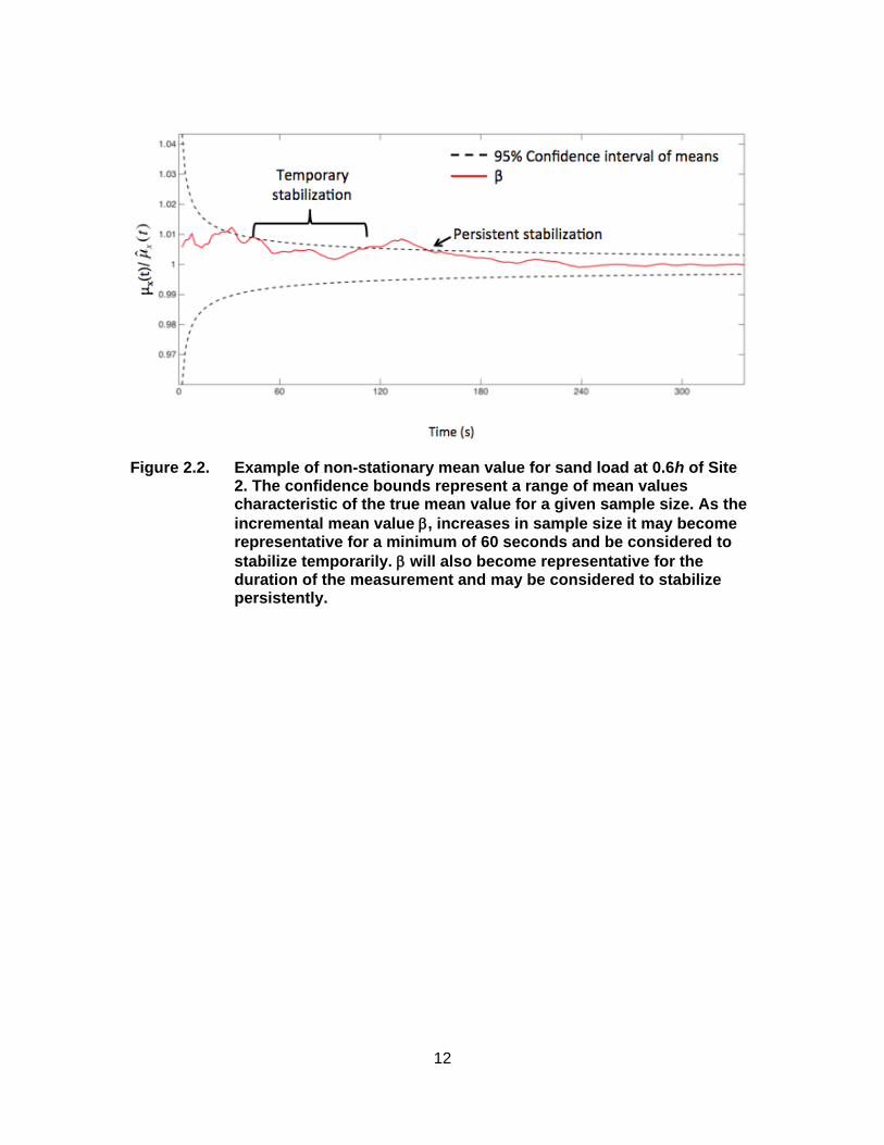
12

Figure 2.2. Example of non-stationary mean value for sand load at 0.6h of Site 2. The confidence bounds represent a range of mean values characteristic of the true mean value for a given sample size. As the

incremental mean value , increases in sample size it may become representative for a minimum of 60 seconds and be considered to

stabilize temporarily. will also become representative for the duration of the measurement and may be considered to stabilize persistently.

13

3.0. Results

3.1. Variability in grain size and concentration

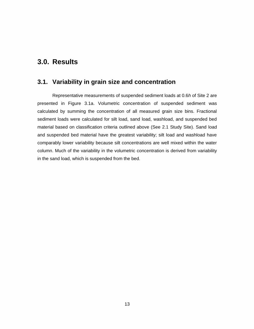
Representative measurements of suspended sediment loads at 0.6h of Site 2 are

presented in Figure 3.1a. Volumetric concentration of suspended sediment was

calculated by summing the concentration of all measured grain size bins. Fractional

sediment loads were calculated for silt load, sand load, washload, and suspended bed

material based on classification criteria outlined above (See 2.1 Study Site). Sand load

and suspended bed material have the greatest variability; silt load and washload have

comparably lower variability because silt concentrations are well mixed within the water

column. Much of the variability in the volumetric concentration is derived from variability

in the sand load, which is suspended from the bed.

14

Figure 3.1. Representative time series at Site 2, 0.6h of a) volumetric concentration, silt load, washload, sand load, and suspended bed material and b) D10, D16, D50, D84, and D90.

Grain size fractions D10, D16, D50, D84, and D90 were calculated at each measured

flow depth for both sites. A representative set of grain size fractions from 0.6h of Site 2 is

presented in Figure 3.1b. D84 has the greatest variability because it represents the

behaviour of the sand load. D90 has comparatively less variability because it is

constrained by the edge of the grain size detector; the largest measured grain size

cannot be larger than 273 µm. D10 and D16 also have less variability because they are

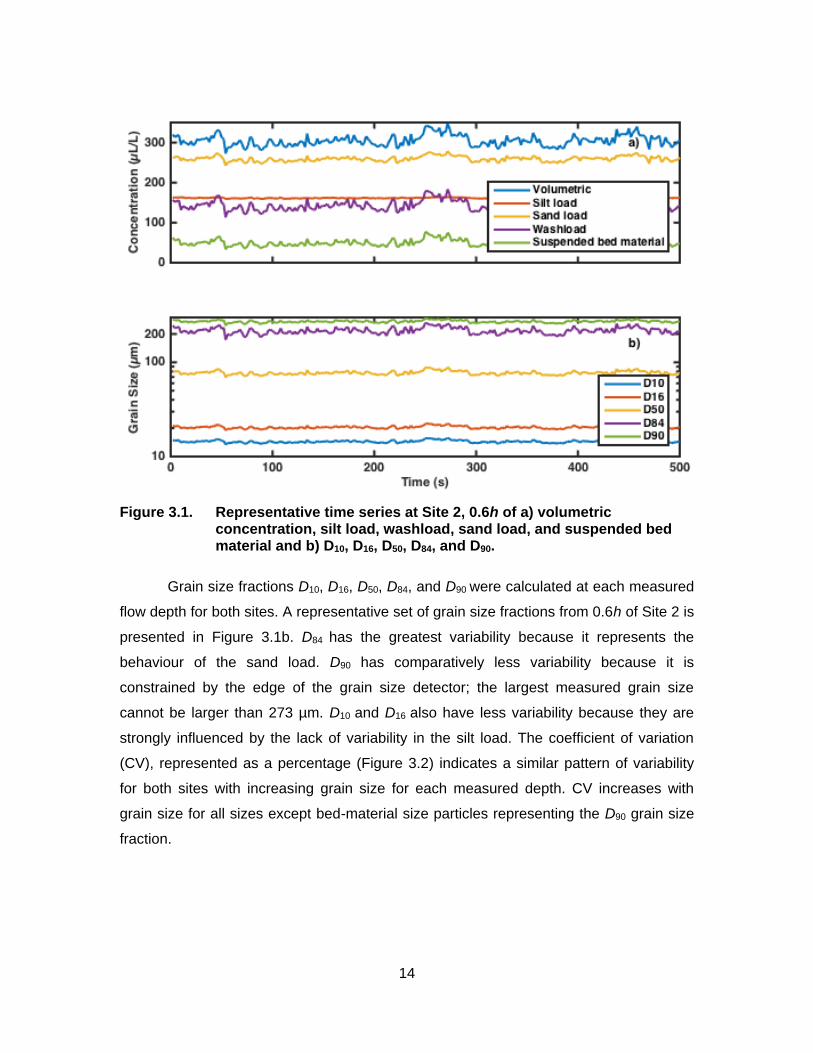
strongly influenced by the lack of variability in the silt load. The coefficient of variation

(CV), represented as a percentage (Figure 3.2) indicates a similar pattern of variability

for both sites with increasing grain size for each measured depth. CV increases with

grain size for all sizes except bed-material size particles representing the D90 grain size

fraction.

15

Figure 3.2. Coefficient of variation for a) Sites 1 and b) 2 computed for each LISST-SL grain size bin.

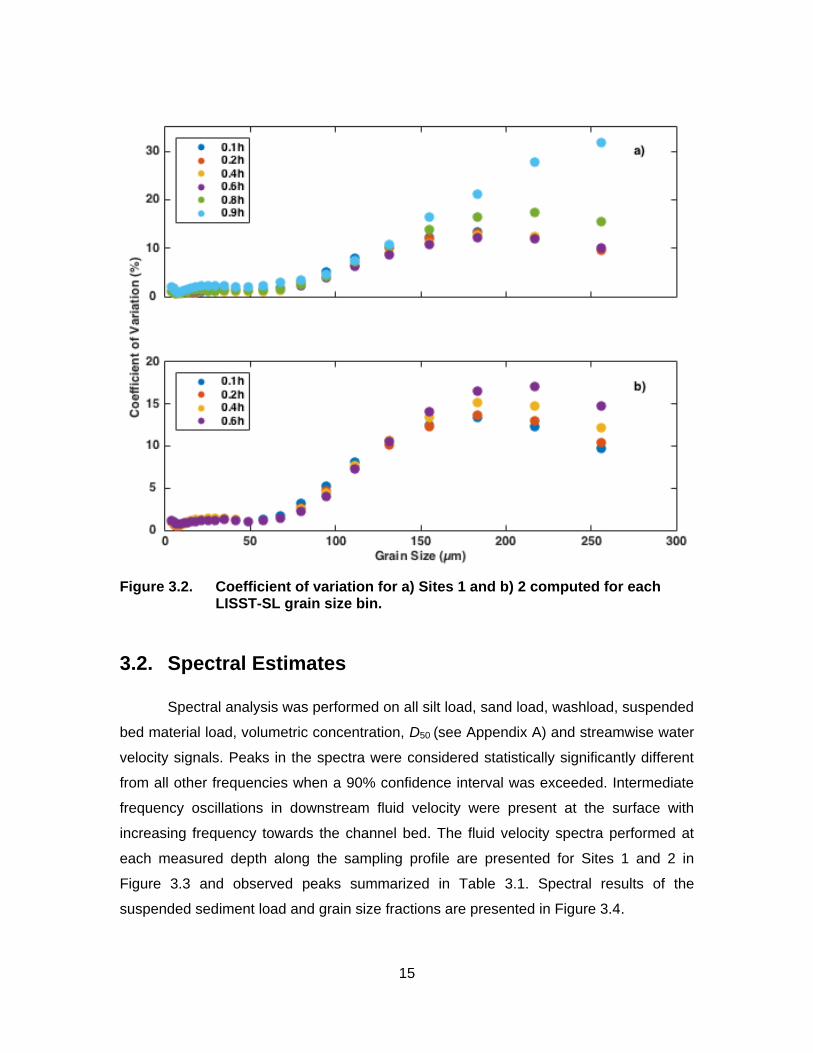
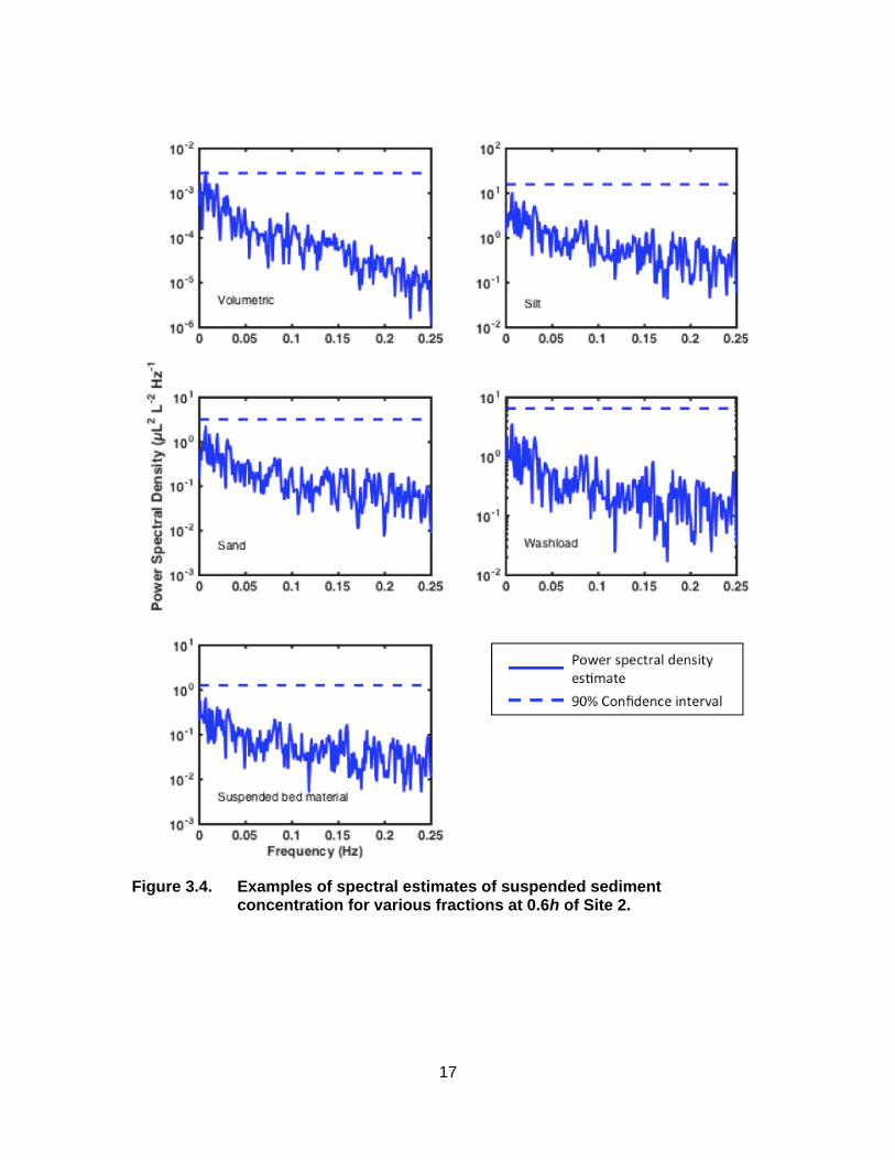
3.2. Spectral Estimates

Spectral analysis was performed on all silt load, sand load, washload, suspended

bed material load, volumetric concentration, D50 (see Appendix A) and streamwise water

velocity signals. Peaks in the spectra were considered statistically significantly different

from all other frequencies when a 90% confidence interval was exceeded. Intermediate

frequency oscillations in downstream fluid velocity were present at the surface with

increasing frequency towards the channel bed. The fluid velocity spectra performed at

each measured depth along the sampling profile are presented for Sites 1 and 2 in

Figure 3.3 and observed peaks summarized in Table 3.1. Spectral results of the

suspended sediment load and grain size fractions are presented in Figure 3.4.

16

Figure 3.3. Spectral estimates of streamwise velocity from Sites 1 and 2 for 0.1h, 0.2h, 0.4h, 0.6h, 0.8h, and 0.9h.

17

Figure 3.4. Examples of spectral estimates of suspended sediment concentration for various fractions at 0.6h of Site 2.

18

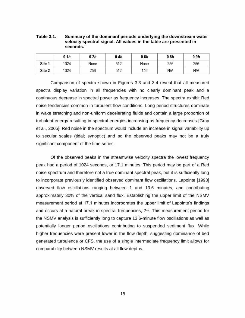
Table 3.1. Summary of the dominant periods underlying the downstream water velocity spectral signal. All values in the table are presented in seconds.

0.1h 0.2h 0.4h 0.6h 0.8h 0.9h

Site 1 1024 None 512 None 256 256

Site 2 1024 256 512 146 N/A N/A

Comparison of spectra shown in Figures 3.3 and 3.4 reveal that all measured

spectra display variation in all frequencies with no clearly dominant peak and a

continuous decrease in spectral power as frequency increases. The spectra exhibit Red

noise tendencies common in turbulent flow conditions. Long period structures dominate

in wake stretching and non-uniform decelerating fluids and contain a large proportion of

turbulent energy resulting in spectral energies increasing as frequency decreases [Gray

et al., 2005]. Red noise in the spectrum would include an increase in signal variability up

to secular scales (tidal; synoptic) and so the observed peaks may not be a truly

significant component of the time series.

Of the observed peaks in the streamwise velocity spectra the lowest frequency

peak had a period of 1024 seconds, or 17.1 minutes. This period may be part of a Red

noise spectrum and therefore not a true dominant spectral peak, but it is sufficiently long

to incorporate previously identified observed dominant flow oscillations. Lapointe [1993]

observed flow oscillations ranging between 1 and 13.6 minutes, and contributing

approximately 30% of the vertical sand flux. Establishing the upper limit of the NSMV

measurement period at 17.1 minutes incorporates the upper limit of Lapointe’s findings

and occurs at a natural break in spectral frequencies, 210. This measurement period for

the NSMV analysis is sufficiently long to capture 13.6-minute flow oscillations as well as

potentially longer period oscillations contributing to suspended sediment flux. While

higher frequencies were present lower in the flow depth, suggesting dominance of bed

generated turbulence or CFS, the use of a single intermediate frequency limit allows for

comparability between NSMV results at all flow depths.

19

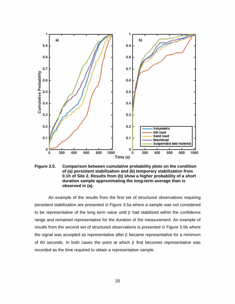
3.3. Cumulative probability of NSMV method

Two versions of the NSMV method applied to the suspended sediment and grain

size fraction data from both sites show the cumulative probability of persistent and

temporary stabilization of the incremental mean value, (Figure 3.5). For suspended

sediment loads represents the cumulative mean concentration, for grain size fractions,

the average value of a particular grain size fraction. As increases in sample size the

value stabilizes on a range of representative mean values within the 95% confidence

interval of the long-term value. is considered to be representative, either temporarily or

persistently, in its relation to the long-term average of the 17.1-minute measurement

period and as such, can only be considered representative after the measurement

period has been analyzed. This measurement period is only a subset of the changing

flow conditions and variable suspended sediment conditions expected over tens of

minutes to hours, much like a bottle sample is a subset of the 17.1-minute measurement

period. The selected measurement period is sufficiently long to average out the short

term fluctuations in sediment concentration and is great enough to capture the longest of

the non-secular flow oscillations identified by Lapointe [1993], thus capturing the

average concentration over an intermediate frequency flow oscillation and ignoring

effects of secular changes. Since a sample was considered representative in relation to

the long duration measurement period, the concentration of one stable representative

sample may differ from that of another due to variations in mean and standard deviation

of their respective measurement period. However, in both cases a sample mean is

considered to be representative based on the population distribution of each respective

measurement period. Since the entire length of the time series was used, a reasonable

estimate of how likely a sample of given length is to be considered representative can be

determined using a cumulative probability plot.

20

Figure 3.5. Comparison between cumulative probability plots on the condition of (a) persistent stabilization and (b) temporary stabilization from 0.1h of Site 2. Results from (b) show a higher probability of a short duration sample approximating the long-term average than is observed in (a).

An example of the results from the first set of structured observations requiring

persistent stabilization are presented in Figure 3.5a where a sample was not considered

to be representative of the long term value until had stabilized within the confidence

range and remained representative for the duration of the measurement. An example of

results from the second set of structured observations is presented in Figure 3.5b where

the signal was accepted as representative after became representative for a minimum

of 60 seconds. In both cases the point at which first becomes representative was

recorded as the time required to obtain a representative sample.

21

Persistent stabilization of requires more time to achieve the same level of

probability compared with temporary stabilization (Figure 3.5). Persistent stabilization of

requires the signal to remain representative for the entire duration of the measurement

and Figure 3.5a shows this requirement is unduly strict. Results show that the probability

of persistent stabilization increases over the whole duration of the sample so that the

longer a sample is measured the more likely it is to represent the long-term value. This

method reveals that the probability of obtaining a representative value is dependent on

the length of the sample, which is not a realistic scenario. It may also be an artifact of the

underlying Red noise observed in the spectrum. This approach minimizes the possibility

that short-term measurements may in fact represent the long-term average. Variability in

the suspended sediment concentration and grain size fractions may push out of the

95% confidence interval even if it had been considered representative for a substantial

period of time. As a result, requirement of persistent stabilization of presupposes

highly probable samples will only be obtained by measuring approximately as long as

the measurement duration

In contrast, temporary stabilization considers whether a shorter duration sample

may accurately reflect the long-term mean, regardless of turbulence after the short

duration sample is collected. This approach shows the probability that a sample

collected by traditional means will accurately reflect the long-term value of interest so

here we focus on temporary stabilization of analysis. Cumulative probability results

under persistent stabilization are presented in Appendix B.

3.4. Temporary stabilization of

3.4.1. Suspended sediment loads

Analysis of the suspended sediment loads with temporary stabilization of the

NSMV yields high probabilities of achieving a stable mean value for shorter

measurement time periods. Cumulative probability plots for suspended sediment loads

of Sites 1 and 2 are presented in Figure 3.6. A short file at 0.6h and non-isokinetically

collected data at 0.9h of Site 1 obscure trends observed at other measurement depths

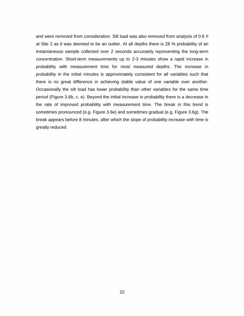
22

and were removed from consideration. Silt load was also removed from analysis of 0.6 h

at Site 2 as it was deemed to be an outlier. At all depths there is 28 % probability of an

instantaneous sample collected over 2 seconds accurately representing the long-term

concentration. Short-term measurements up to 2-3 minutes show a rapid increase in

probability with measurement time for most measured depths. The increase in

probability in the initial minutes is approximately consistent for all variables such that

there is no great difference in achieving stable value of one variable over another.

Occasionally the silt load has lower probability than other variables for the same time

period (Figure 3.6b, c, e). Beyond the initial increase in probability there is a decrease in

the rate of improved probability with measurement time. The break in this trend is

sometimes pronounced (e.g. Figure 3.6e) and sometimes gradual (e.g. Figure 3.6g). The

break appears before 8 minutes, after which the slope of probability increase with time is

greatly reduced.

23

Figure 3.6. Cumulative probability plots of suspended sediment loads with the

condition of temporary stabilization of the signal. Measurements from Site 1 at a) 0.1h, b) 0.2h, c) 0.4h, d) 0.8h, and Site 2 at e) 0.1h, f) 0.2h, g) 0.4h, and h) 0.6h show the cumulative probability of obtaining a sample with a representative grain size moment value when measuring for a given period of time.

24

3.4.2. Grain size fractions

Similar results are observed in the grain size fraction analysis of the NSMV

presented in Figure 3.7 for Sites 1 and 2. Also similar to the previous set of results is that

0.6h and 0.9h were omitted from further consideration. Instantaneous samples indicate

an 18 – 38 % probability of obtaining a representative value in 2 seconds of sampling,

after which there is a rapid increase in the probability. The increase in probability is

followed by a transition to lower rates of probability increase with time. The transition

occurs, again, between ~2 and 8 minutes. Even more so than for suspended sediment

loads, grain size fractions at all depths typically achieve an approximately similar level of

probability in representing the long-term value at about the same measurement time.

25

Figure 3.7. Cumulative probability plots of grain size fractions with the

condition of temporary stabilization of the signal. Measurements from Site 1 at a) 0.1h, b) 0.2h, c) 0.4h, d) 0.8h, and Site 2 at e) 0.1h, f) 0.2h, g) 0.4h, and h) 0.6h show the cumulative probability of obtaining a sample with a representative grain size moment value when measuring for a given period of time.

26

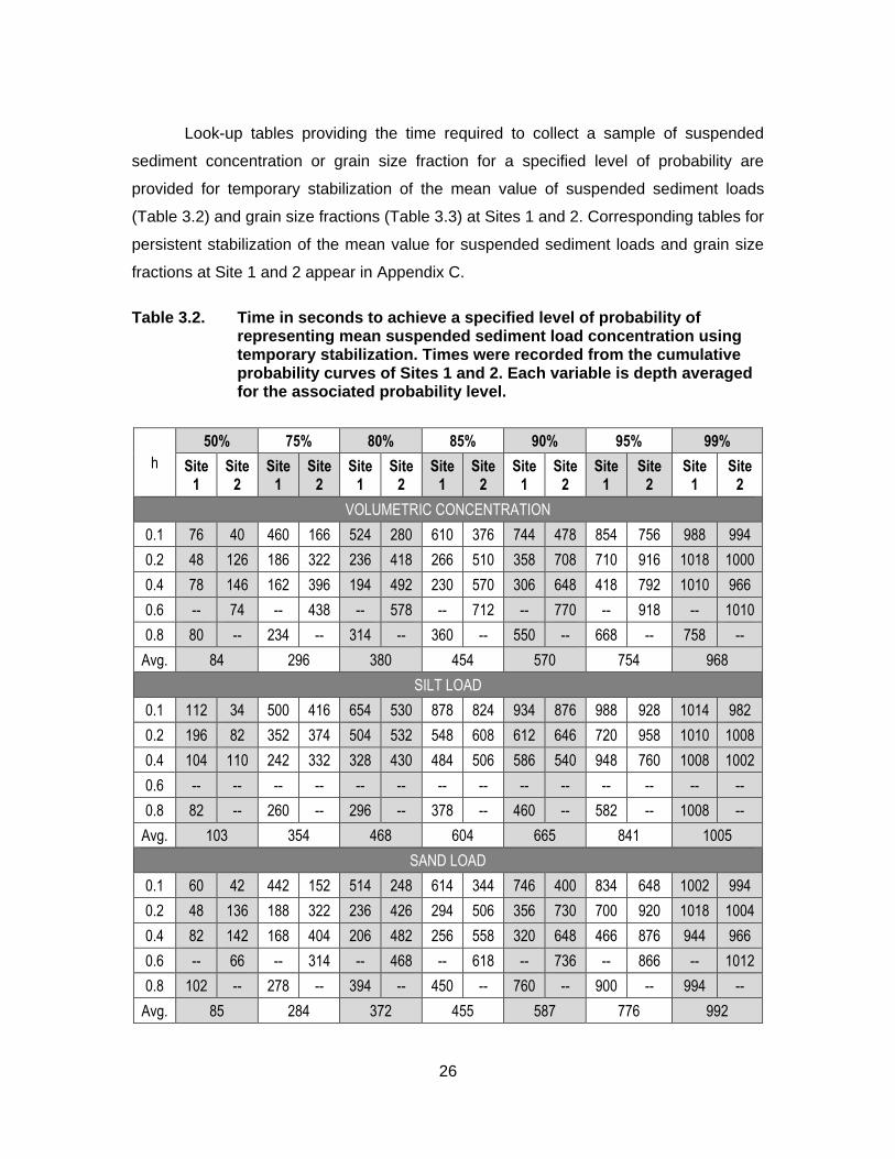
Look-up tables providing the time required to collect a sample of suspended

sediment concentration or grain size fraction for a specified level of probability are

provided for temporary stabilization of the mean value of suspended sediment loads

(Table 3.2) and grain size fractions (Table 3.3) at Sites 1 and 2. Corresponding tables for

persistent stabilization of the mean value for suspended sediment loads and grain size

fractions at Site 1 and 2 appear in Appendix C.

Table 3.2. Time in seconds to achieve a specified level of probability of representing mean suspended sediment load concentration using temporary stabilization. Times were recorded from the cumulative probability curves of Sites 1 and 2. Each variable is depth averaged for the associated probability level.

h

50% 75% 80% 85% 90% 95% 99%

Site 1

Site 2

Site 1

Site 2

Site 1

Site 2

Site 1

Site 2

Site 1

Site 2

Site 1

Site 2

Site 1

Site 2

VOLUMETRIC CONCENTRATION

0.1 76 40 460 166 524 280 610 376 744 478 854 756 988 994

0.2 48 126 186 322 236 418 266 510 358 708 710 916 1018 1000

0.4 78 146 162 396 194 492 230 570 306 648 418 792 1010 966

0.6 -- 74 -- 438 -- 578 -- 712 -- 770 -- 918 -- 1010

0.8 80 -- 234 -- 314 -- 360 -- 550 -- 668 -- 758 --

Avg. 84 296 380 454 570 754 968

SILT LOAD

0.1 112 34 500 416 654 530 878 824 934 876 988 928 1014 982

0.2 196 82 352 374 504 532 548 608 612 646 720 958 1010 1008

0.4 104 110 242 332 328 430 484 506 586 540 948 760 1008 1002

0.6 -- -- -- -- -- -- -- -- -- -- -- -- -- --

0.8 82 -- 260 -- 296 -- 378 -- 460 -- 582 -- 1008 --

Avg. 103 354 468 604 665 841 1005

SAND LOAD

0.1 60 42 442 152 514 248 614 344 746 400 834 648 1002 994

0.2 48 136 188 322 236 426 294 506 356 730 700 920 1018 1004

0.4 82 142 168 404 206 482 256 558 320 648 466 876 944 966

0.6 -- 66 -- 314 -- 468 -- 618 -- 736 -- 866 -- 1012

0.8 102 -- 278 -- 394 -- 450 -- 760 -- 900 -- 994 --

Avg. 85 284 372 455 587 776 992

27

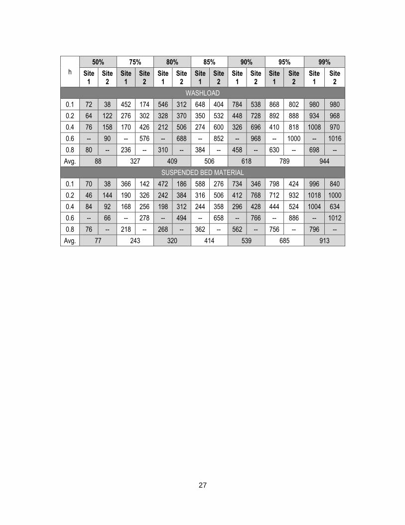
h

50% 75% 80% 85% 90% 95% 99%

Site 1

Site 2

Site 1

Site 2

Site 1

Site 2

Site 1

Site 2

Site 1

Site 2

Site 1

Site 2

Site 1

Site 2

WASHLOAD

0.1 72 38 452 174 546 312 648 404 784 538 868 802 980 980

0.2 64 122 276 302 328 370 350 532 448 728 892 888 934 968

0.4 76 158 170 426 212 506 274 600 326 696 410 818 1008 970

0.6 -- 90 -- 576 -- 688 -- 852 -- 968 -- 1000 -- 1016

0.8 80 -- 236 -- 310 -- 384 -- 458 -- 630 -- 698 --

Avg. 88 327 409 506 618 789 944

SUSPENDED BED MATERIAL

0.1 70 38 366 142 472 186 588 276 734 346 798 424 996 840

0.2 46 144 190 326 242 384 316 506 412 768 712 932 1018 1000

0.4 84 92 168 256 198 312 244 358 296 428 444 524 1004 634

0.6 -- 66 -- 278 -- 494 -- 658 -- 766 -- 886 -- 1012

0.8 76 -- 218 -- 268 -- 362 -- 562 -- 756 -- 796 --

Avg. 77 243 320 414 539 685 913

28

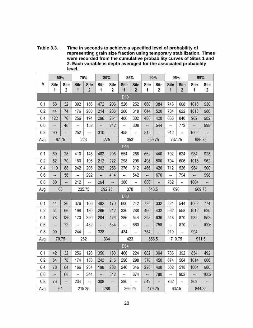
Table 3.3. Time in seconds to achieve a specified level of probability of representing grain size fraction using temporary stabilization. Times were recorded from the cumulative probability curves of Sites 1 and 2. Each variable is depth averaged for the associated probability level.

h

50% 75% 80% 85% 90% 95% 99%

Site 1

Site 2

Site 1

Site 2

Site 1

Site 2

Site 1

Site 2

Site 1

Site 2

Site 1

Site 2

Site 1

Site 2

D10

0.1 58 32 392 156 472 206 526 252 660 384 748 608 1016 930

0.2 44 74 176 200 214 236 260 318 644 520 734 622 1018 986

0.4 122 76 256 194 296 254 400 302 488 420 666 840 962 982

0.6 -- 46 -- 158 -- 212 -- 308 -- 544 -- 772 -- 998

0.8 90 -- 252 -- 310 -- 458 -- 818 -- 912 -- 1002 --

Avg. 67.75 223 275 353 559.75 737.75 986.75

D16

0.1 60 28 410 148 482 206 554 258 662 440 792 624 984 928

0.2 52 70 180 196 212 222 298 298 498 500 704 606 1018 962

0.4 110 88 242 206 282 256 376 312 466 426 712 526 964 900

0.6 -- 56 -- 292 -- 414 -- 542 -- 676 -- 794 -- 998

0.8 80 -- 212 -- 264 -- 386 -- 680 -- 762 -- 1004 --

Avg. 68 235.75 292.25 378 543.5 690 969.75

D50

0.1 44 26 376 106 482 170 600 242 738 332 824 544 1002 774

0.2 54 66 198 180 266 212 330 288 460 432 562 558 1012 620

0.4 78 136 170 390 204 476 286 544 358 636 548 870 932 952

0.6 -- 72 -- 432 -- 534 -- 660 -- 758 -- 870 -- 1006

0.8 90 -- 244 -- 328 -- 434 -- 754 -- 910 -- 994 --

Avg. 70.75 262 334 423 558.5 710.75 911.5

D84

0.1 42 32 256 126 350 160 466 224 682 304 786 392 854 492

0.2 54 78 174 188 242 216 296 298 370 450 674 564 1014 606

0.4 78 84 166 234 198 288 246 346 298 408 502 518 1004 980

0.6 -- 68 -- 344 -- 542 -- 674 -- 780 -- 902 -- 1002

0.8 76 -- 234 -- 308 -- 380 -- 542 -- 762 -- 802 --

Avg. 64 215.25 288 366.25 479.25 637.5 844.25

29

h

50% 75% 80% 85% 90% 95% 99%

Site 1

Site 2

Site 1

Site 2

Site 1

Site 2

Site 1

Site 2

Site 1

Site 2

Site 1

Site 2

Site 1

Site 2

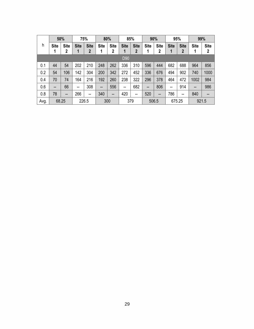
D90

0.1 44 54 202 210 248 262 336 310 596 444 682 688 964 856

0.2 54 106 142 304 200 342 272 452 336 676 494 902 740 1000

0.4 70 74 164 216 192 260 238 322 296 378 464 472 1002 984

0.6 -- 66 -- 308 -- 556 -- 682 -- 806 -- 914 -- 986

0.8 78 -- 266 -- 340 -- 420 -- 520 -- 786 -- 840 --

Avg. 68.25 226.5 300 379 506.5 675.25 921.5

30

4.0. Discussion

Do current point-sample measurement techniques adequately capture a representative value of suspended sediment?

According to the Water Survey of Canada Field Guide, the time required to fill a

quart-sized bottle with a USGS standard P-63 at flows averaging 1.0 – 1.8 m s-1 as

observed during our data collection, is 20 – 41 seconds [Tassone and Lapointe, 1999].

According to our findings a measurement in this time period presents on average 35 –

45% probability of accurately reflecting the long-term mean concentration or grain size

fraction. Times presented in Tables 3.2 and 3.3 for each variable are depth averaged to

obtain a single estimate of sample duration for a given level of probability. Collection of

the volumetric concentration with 90% confidence of accurately representing the mean

value requires 570 seconds (9.5 minutes) of sampling. Alternatively stated, if one were

to collect ten 9.5 minutes samples, one of those samples is likely to be unrepresentative.

If two bottle samples of volumetric concentration were collected to represent the mean

concentration, each 40 seconds in length, statistically, only one of the bottles would

accurately represent the mean concentration. Clearly, the time averaging performed

during the collection of a standard bottle sample is insufficient to accurately reflect the

long-term mean value. Inadequate time averaging as a source of error in depth-

integrated bottle sampling identified in Topping et al. [2011] also influences point-sample

measurements. Typical short-duration bottle samples capture some of the variability of

the long-term average but do not guarantee a representative sample. Topping et al.

[2011] recommended adding a second transit, which by sampling the same location

twice improves time averaging at every point in the flow. In point sample measurements,

time averaging at a single point is considerably greater than in depth-integration but it is

clear that the time averaging performed during a single sample is not long enough.

Therefore, the results suggest that current bottle sampling practices are insufficient to

capture the true mean concentration or grain size fraction in suspension. The probability

of a single bottle sample accurately reflecting the mean concentration or grain size

31

fraction is too low to consider that the current methods are a reasonable sampling

approach and is one of the reasons for the customary large scatter in suspended

sediment rating curves. Increasing the time period over which suspended sediment is

measured therefore seems to be the most appropriate way to improve the probability of

representing the long-term mean concentration or grain size fraction.

What sample duration is required to obtain an accurate mean concentration? Does the time required to obtain a representative mean concentration vary for different components of the suspended sediment load?

Guaranteeing certainty in a measurement accurately reflecting the long-term

value is difficult. Long-duration measurements are equal to the measurement period and

are the best approach to accurately representing the long-term value but due to

exceedingly long measurement times this is impractical. Assuming a lower probability

still requires exceptionally long sample durations; a total of nineteen bottle samples,

each collecting 30 seconds of water-sediment mixture would be required to provide a

90% probability of accurately representing the mean concentration of volumetric

concentration. Currently a single bottle sample is used for each point in the water

column to provide the mean concentration. Results from these structured observations

indicate this approach may be accurate in <50% of samples. The results also indicate

that the probability of obtaining a representative mean concentration or grain size

moment is approximately the same for all variables meaning the same measurement

period may be appropriate for all components of the suspended sediment load and all

grain size fractions. Improving the probability of representing the long-term value in the

shortest period of time would bridge the gap between short duration, moderately

probable estimates of the long-term value and prohibitively long, but certain

measurements.

By locating the point of diminishing returns on the cumulative probability curves

we are able to determine a sampling time adequate to maximize sampling efficiency

while minimizing sampling time. Finding this point of diminishing returns in sampling time

is accomplished by identifying the break in slope along each line of cumulative

probability. In all plots there is an immediate increase in probability for the first 2 minutes

and a lower rate of increase beyond the 8-minute mark. The point of diminishing returns

32

occurs between these two periods. Measuring the slope of each of these segments and

identifying the point at which they intersect identifies the point of diminishing returns.

This point indicates the most efficient duration over which to sample and the probability

associated with the measurement time is obtained from the cumulative probability curve.

Using the point of diminishing returns a depth-averaged value of the most

efficient sampling time can be reached. The most efficient sample of volumetric

concentration will be collected by 264 seconds with 73% probability of accurately

representing the mean. For D50 a sample must be 240 seconds long to achieve 75%

probability. Summary of all other variables can be found in Appendix D. The method

involving the point of diminishing returns does not indicate how long a sample should be

collected for but rather indicates the shortest sample duration likely to ensure the

greatest probability of accurately reflecting the mean concentration of grain size fraction

of interest.

The length of sample required to accurately represent the mean concentration of

a suspended sediment load or a particular grain size fraction depends on the level of

probability desired. Since individual bottle samples bear a low probability of representing

the mean value, requiring multiple bottles totalling between 9 and 12 minutes of sample

duration to accurately reflect the mean, it becomes evident that bottle sampling may not

be the most efficient method of sampling suspended sediment. This research indicates

that longer duration sampling through alternative means may prove more effective while

being less time consuming and resource demanding than traditional bottle sampling.

Collection of continuous suspended sediment data has been successfully documented

using acoustic monitoring [Attard et al., 2014]. Pressure-difference techniques [Gray and

Landers, 2014] may also provide continuous data. Laser-diffraction, used in this

research, also provides continuous concentration data.

33

5.0. Conclusion

Long duration measurements of suspended sediment concentration were

examined from the Fraser River, British Columbia, Canada. Continuous hour-long time

series data of suspended sediment concentration and grain size distribution were

collected along two sampling profiles based on a standard sampling profile. Average

discharge was 8265 m3 s-1 during the measurement period May 30 – June 2, 2013. A

probability-based approach determined the likelihood of a sample of suspended

sediment accurately reflecting the long-term value of mean concentration or grain size

fraction. Results indicate that typical bottle samples of <60 seconds in duration bear a

low to moderate probability of accurately representing the long-term value. Improving the

probability to 90 % of accurately reflecting the mean concentration of volumetric

concentration requires 9.5 minutes of sampling duration. All components of the

suspended load and grain size fractions bear approximately the same likelihood of

representing the long-term value for any given time period. The results indicate that

current bottle sampling measurement techniques inadequately time-average over the

variability in suspended sediment concentration and do no reliably provide a

representative mean concentration.

34

References

Adrian, R. J., and Marusic, I. (2012). Coherent structures in flow over hydraulic engineering surfaces. Journal of Hydraulic Research, 50:5, 451–464.

Adrian, R. J. (2013). Structure of Turbulent Boundary Layers. In Coherent Flow Structures at Earth’s Surface (pp. 17–24).

Attard, M. E. (2012). Evaluation of ADCPs for suspended sediment transport monitoring, Fraser River, British Columbia. MSc thesis, Simon Fraser University.

Attard, M. E., Venditti, J. G., and Church, M. (2014). Suspended sediment transport in Fraser River at Mission, British Columbia: New observations and comparison to historical records. Canadian Water Resources Journal / Revue Canadienne Des Ressources Hydriques, 39(3), 356–371. doi:10.1080/07011784.2014.942105

Bendat, J. S., and Piersol, A. G. (1966). Measurement and analysis of random data. USA: John Wiley and Sons. (pp. 337 – 344)

Bradley, R. W., Venditti, J. G., Kostaschuk, R. A., Hendershot, M., Church, M., and Columbia, B. (2013). Flow and sediment suspension events over low-angle dunes : Fraser Estuary, Canada. Journal of Geophysical Research. 118, 1693-1709, doi:10.1002/jgrf.20118

Bridge, J. S. (2003). Rivers and floodplains: forms, processes, and sedimentary record. USA: Blackwell Science Ltd. (pp. 55 – 56)

Church, M. (2006). Bed Material Transport and the Morphology of Alluvial River Channels. Annual Review of Earth and Planetary Sciences, 34(1), 325–354. doi:10.1146/annurev.earth.33.092203.122721

Dashtgard, S. E., Venditti, J. G., Hill, P. R., Sisulak, C. F., Johnson, S. M., and La Croix, A. D. (2012). Sedimentation across the tidal-fluvial transition in the lower Fraser River, Canada. The Sedimentary Record, 4–9. doi: 10.2110/sedred.2012.4

Domarad, N. (2011). Flow and suspended sediment transport through the gravel-sand transition in the Fraser River, British Columbia. M.Sc. thesis, Simon Fraser University.

35

Hutchins, N., and Marusic, I. (2007). Evidence of very long meandering features in the logarithmic region of turbulent boundary layers. Journal of Fluid Mechanics, 579, 1. doi:10.1017/S0022112006003946

Gray, T. E., Alexander, J., & Leeder, M. R. (2005). Quantifying velocity and turbulence structure in depositing sustained turbidity currents across breaks in slope. Sedimentology, 52(3), 467–488. doi:10.1111/j.1365-3091.2005.00705.x

Gray, J. R. and Landers, M. N. (2014). Measuring suspended sediment. In Ahuja, S., editor, Comprehensive Water Quality and Purification. Amsterdam, Elsevier, vol. 1, 157-204.

Kline, S. J., Reynolds, W. C., Schraub, F. A., and Rundstadler, P. W. (1967). The structure of turbulent boundary layers. Journal of Fluid Mechanics, 30, 741–773.

Kostaschuk, R. a., and Church, M. a. (1993). Macroturbulence generated by dunes: Fraser River, Canada. Sedimentary Geology, 85, 25–37. doi:10.1016/0037-0738(93)90073-E

Kostaschuk, R., and Best, J. (2005). Response of sand dunes to variations in tidal flow: Fraser Estuary, Canada. Journal of Geophysical Research, 110. doi:10.1029/2004JF000176

Kwoll, E., Becker, M., and Winter, C. (2014). With or against the tide: The influence of bed form asymmetry on the formation of Macroturbulence and suspended sediment patterns. Water Resources Research, 2108–2123. doi:10.1002/2012WR013085.

Lapointe, M. (1992). Burst-like sediment suspension events in a sand bed river. Earth Surface Processes and Landforms, 17(3), 253–270. doi:10.1002/esp.3290170305

Lapointe, M. (1993). Monitoring alluvial sand suspension by eddy correlation. Earth Surface Processes and Landforms, 18, 157–175. doi: 10.1002/esp.3290180207

Lapointe, M. F. (1996). Frequency spectra and intermittency of the turbulent suspension process in a sand-bed river. Sedimentary Geology, 43, 439–449. doi:10.1046/j.1365-3091.1996.d01-18.x

Marquis, G. A., & Roy, A. G. (2013). From macroturbulent flow structures to large‐ scale flow pulsations in gravel‐ bed rivers. Coherent Flow Structures at Earth's Surface, (pp. 261-274).

McLean, D. G., Church, M., and Tassone, B. (1999). Sediment transport along lower Fraser River: 1. Measurements and hydraulic computations. Water Resources Research, 35(8), 2533. doi:10.1029/1999WR900101

36

Menke, W., and Menke, J. (2012). Environmental data analysis with MATLAB. USA: Elsevier. (pp. 229 – 234).

Milliman, J. D., and Meade, R. H. (1983). World-wide delivery of river sediment to the oceans. The Journal of Geology. doi:10.1086/628741

Milliman, J. D., and Syvitski, J. P. M. (1992). Geomorphic/tectonic control of sediment discharge to the ocean: the importance of small mountainous rivers. Journal of Geology, 100, 325–344.

Schmid, H. (2012). How to use the FFT and Matlab’s pwelch function for signal and noise simulations and measurements. [Report]. Retrieved from http://www.fhnw.ch/technik/ime/publikationen/2012/how-to-use-the-fft-and-matlab2019s-pwelch-function-for-signal-and-noise-simulations-and-measurements (accessed on 10 July, 2014).

Sequoia Scientific Inc. (2013). LISST-SL V2.1 Operating manual. Retrieved from http://www.sequoiasci.com/wp-content/uploads/2013/07/LISST-SLUsersManual_v2.1.pdf (accessed on 5 May, 2013).

Shugar, D. H., Kostaschuk, R., Best, J. L., Parsons, D. R., Lane, S. N., Orfeo, O., and Hardy, R. J. (2010). On the relationship between flow and suspended sediment transport over the crest of a sand dune, Río Paraná, Argentina. Sedimentology, 57(1), 252–272. doi:10.1111/j.1365-3091.2009.01110.x

Soulsby, R. (1980). Selecting record length and digitization rate for near-bed turbulence measurements. Journal of Physical Oceanography, 10, 208–219.

Syvitski, J. P., Vörösmarty, C. J., Kettner, A. J., & Green, P. (2005). Impact of humans on the flux of terrestrial sediment to the global coastal ocean. Science, 308(5720), 376-380.

Tassone, B., and Lapointe, F. (1999). Suspended-sediment sampling. Hydrometric technician career development program. The Water Survey of Canada. Retrieved from http://publications.gc.ca/collections/collection_2014/ec/En56-247-1999-eng.pdf (accessed 17 February, 2015).

Topping, D. J., Rubin, D.M., Wright, S.A., Melis, T. S. (2011). Field Evaluation of the Error Arising from Inadequate Time Averaging in the Standard Use of Depth-Integrating Suspended-Sediment Samplers. (No. 1774, pp.i-95). US Geological Survey.

Venditti, J. G., and Church, M. (2014). Morphology and controls on the position of a gravel-sand transition: Fraser River, British Columbia. Journal of Geophysical Research, 1959–1976. doi:10.1002/2014JF003147.

37

Venditti, J. G., Domarad, N., Church, M., & Rennie, C. D. (2015). The Gravel‐ sand transition: Sediment dynamics in a diffuse extension. Journal of Geophysical Research: Earth Surface. doi: 10.1002/2014JF003328.

38

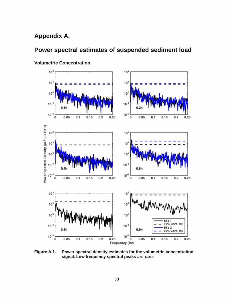
Appendix A. Power spectral estimates of suspended sediment load

Volumetric Concentration

Figure A.1. Power spectral density estimates for the volumetric concentration signal. Low frequency spectral peaks are rare.

39

Silt load

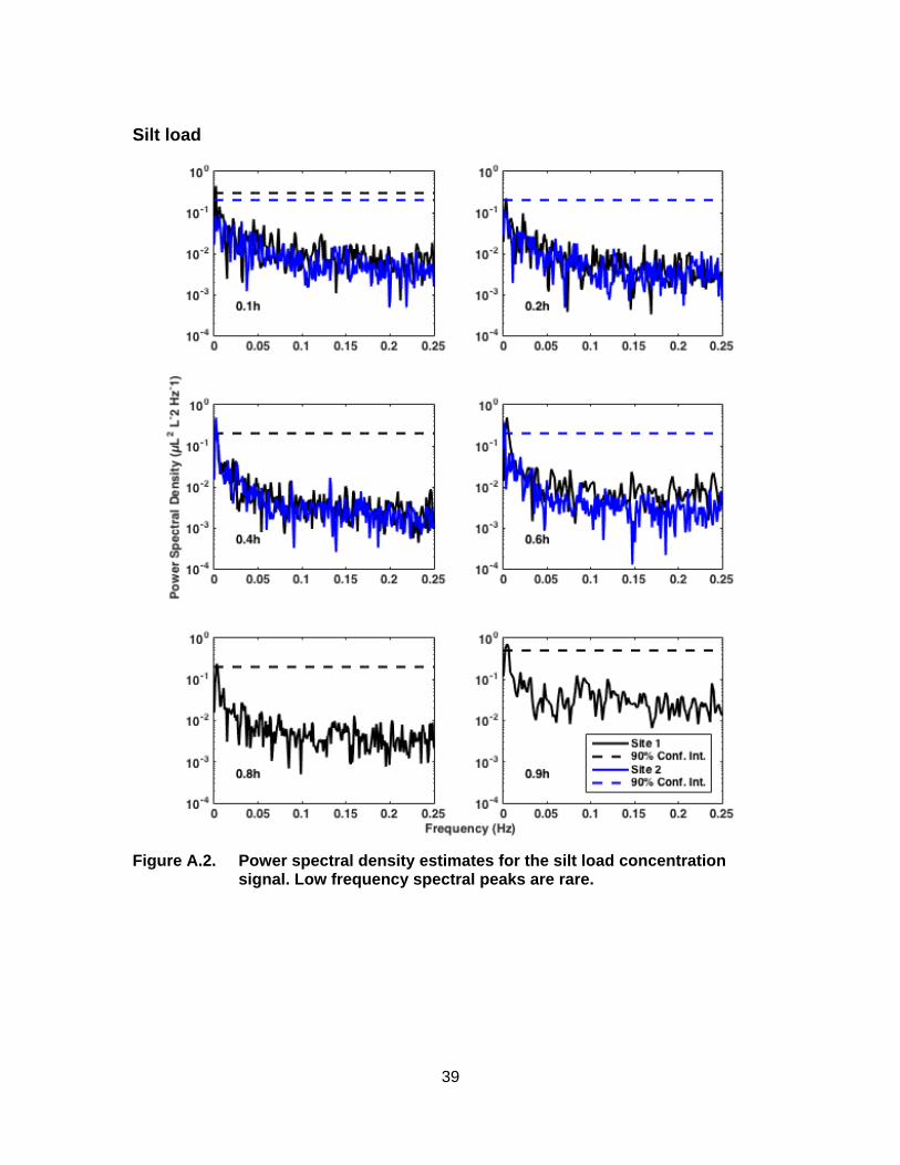
Figure A.2. Power spectral density estimates for the silt load concentration signal. Low frequency spectral peaks are rare.

40

Sand load

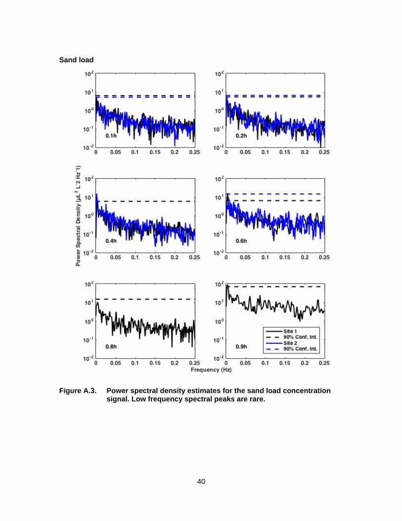
Figure A.3. Power spectral density estimates for the sand load concentration signal. Low frequency spectral peaks are rare.

41

Washload

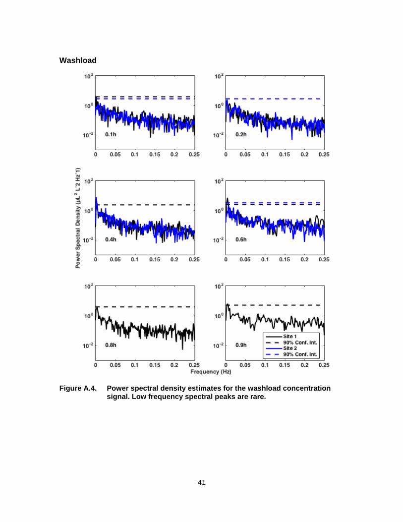
Figure A.4. Power spectral density estimates for the washload concentration signal. Low frequency spectral peaks are rare.

42

Suspended bed material

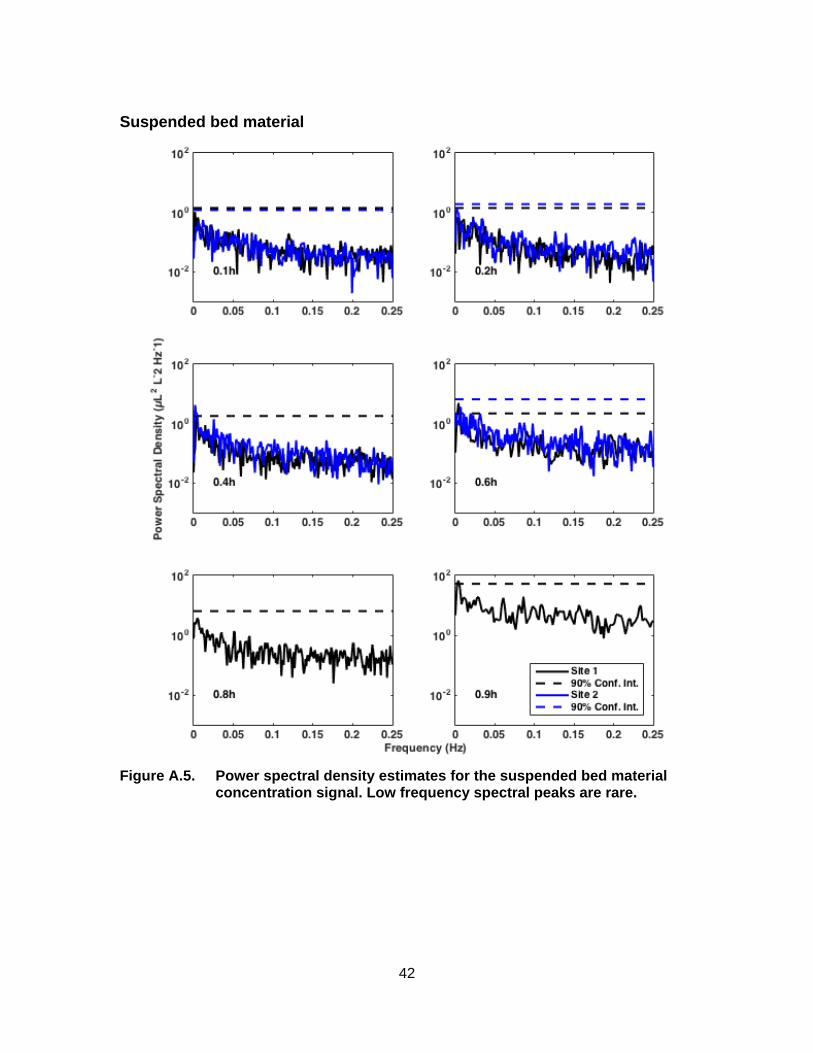
Figure A.5. Power spectral density estimates for the suspended bed material concentration signal. Low frequency spectral peaks are rare.

43

D50

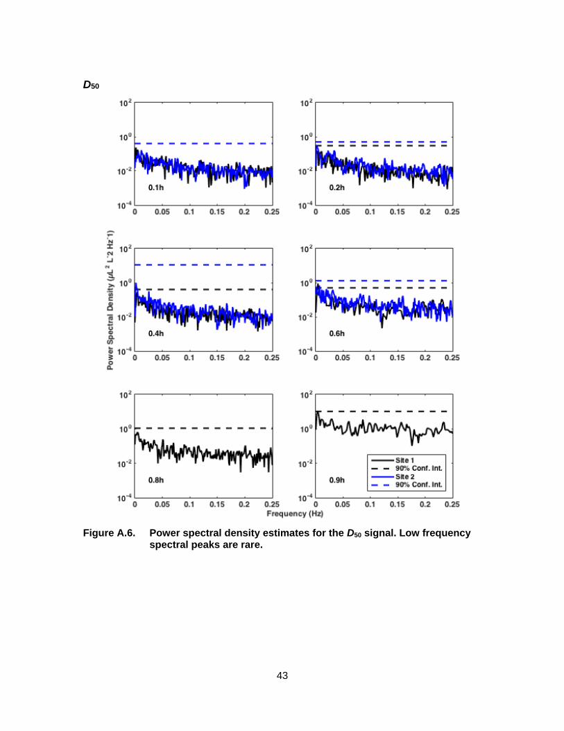
Figure A.6. Power spectral density estimates for the D50 signal. Low frequency spectral peaks are rare.

44

Appendix B.

Persistent stabilization of

45

Suspended sediment loads

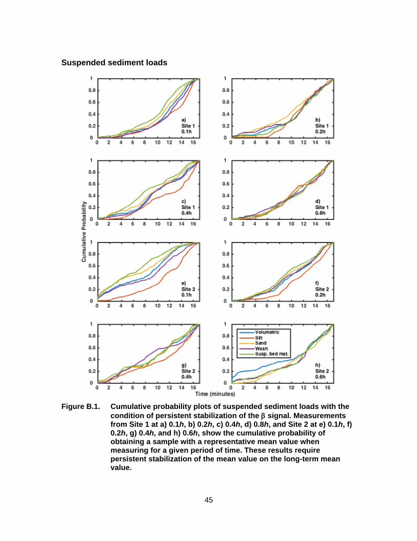
Figure B.1. Cumulative probability plots of suspended sediment loads with the

condition of persistent stabilization of the signal. Measurements from Site 1 at a) 0.1h, b) 0.2h, c) 0.4h, d) 0.8h, and Site 2 at e) 0.1h, f) 0.2h, g) 0.4h, and h) 0.6h, show the cumulative probability of obtaining a sample with a representative mean value when measuring for a given period of time. These results require persistent stabilization of the mean value on the long-term mean value.

46

Grain size fractions

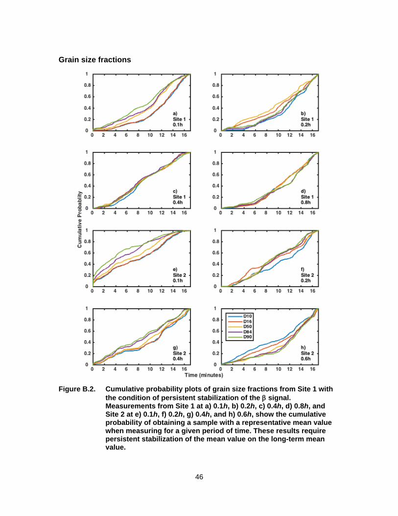
Figure B.2. Cumulative probability plots of grain size fractions from Site 1 with

the condition of persistent stabilization of the signal. Measurements from Site 1 at a) 0.1h, b) 0.2h, c) 0.4h, d) 0.8h, and Site 2 at e) 0.1h, f) 0.2h, g) 0.4h, and h) 0.6h, show the cumulative probability of obtaining a sample with a representative mean value when measuring for a given period of time. These results require persistent stabilization of the mean value on the long-term mean value.

47

Appendix C. Sampling time for a specified level of probability

Suspended sediment loads

h

50% 75% 80% 85% 90% 95% 99%

Site 1

Site 2

Site 1

Site 2

Site 1

Site 2

Site 1

Site 2

Site 1

Site 2

Site 1

Site 2

Site 1

Site 2

VOLUMETRIC CONCENTRATION

0.1 724 506 852 738 874 764 890 804 914 838 950 900 1020 956

0.2 712 706 852 884 864 904 902 926 946 948 1002 968 1016 1008

0.4 602 702 860 870 880 898 900 944 946 980 986 998 1010 1016

0.6 680 838 878 934 968 980 1000

0.8 668 858 892 916 946 972 1010

Avg. 662.5 844 869.25 902 935.75 969.5 1004.5

SILT LOAD

0.1 810 502 910 720 928 754 942 786 952 830 972 888 1004 944

0.2 694 574 832 864 892 884 916 902 944 932 968 962 1020 1004

0.4 812 700 932 844 952 894 968 922 984 964 1000 982 1018 1010

0.6 720 882 914 960 990 1002 1018

0.8 638 880 904 924 944 974 1022

Avg. 681.25 858 890.25 915 942.5 968.5 1005

SAND LOAD

0.1 690 262 824 528 846 576 872 686 898 758 934 818 1018 956

0.2 638 560 820 832 846 856 884 878 950 890 998 930 1020 1008

0.4 590 558 820 764 848 838 882 886 902 918 952 940 1010 994

0.6 754 886 918 948 970 982 1006

0.8 664 854 886 912 948 976 1012

Avg. 589.5 791 826.75 868.5 904.25 941.25 1003

WASHLOAD

0.1 754 396 878 654 900 690 914 728 934 766 966 838 1016 930

0.2 714 538 834 820 868 862 894 892 952 922 1002 968 1014 1012

0.4 600 626 872 818 894 882 928 924 964 968 990 988 1014 1014

0.6 760 872 898 938 974 990 1012

0.8 722 898 926 938 952 976 1016

Avg. 638.75 830.75 865 894.5 929 964.75 1003.5

48

h

50% 75% 80% 85% 90% 95% 99%

Site 1

Site 2

Site 1

Site 2

Site 1

Site 2

Site 1

Site 2

Site 1

Site 2

Site 1

Site 2

Site 1

Site 2

SUSPENDED BED MATERIAL

0.1 656 202 768 524 792 588 826 638 870 706 926 820 1018 982

0.2 712 538 870 800 892 830 922 852 964 888 996 916 1018 1006

0.4 494 536 784 768 830 808 856 884 886 916 918 946 1012 1002

0.6 772 900 932 960 976 984 1000

0.8 728 860 898 926 958 988 1010

Avg. 579.75 784.25 821.25 858 895.5 936.75 1006

Table C.1. Time in seconds to achieve a specified level of probability of representing mean suspended sediment load concentration using persistent stabilization. Times were recorded from the cumulative probability curves of Sites 1 and 2. Each variable is depth averaged for the associated probability level

49

Grain size fractions

h

50% 75% 80% 85% 90% 95% 99%

Site 1

Site 2

Site 1

Site 2

Site 1

Site 2

Site 1

Site 2

Site 1

Site 2

Site 1

Site 2

Site 1

Site 2

D10

0.1 758 506 884 738 902 764 920 804 948 838 976 900 1012 956

0.2 744 706 898 884 916 904 938 926 962 948 998 968 1020 1008

0.4 522 702 788 870 816 898 854 944 886 980 926 998 1008 1016

0.6 680 838 878 934 968 980 1000

0.8 678 856 886 914 942 974 1004

Avg. 662 844.5 870.5 904.25 934 965 1003

D16

0.1 754 502 876 720 888 754 914 786 934 830 970 888 1012 944

0.2 652 574 870 574 888 574 920 574 952 574 990 574 1020 574

0.4 520 700 778 700 818 700 846 700 874 700 916 700 1002 700

0.6 720 720 720 720 720 720 720

0.8 674 860 890 926 958 982 1008

Avg. 637 762.25 779 798.25 817.75 842.5 872.5

D50

0.1 654 396 784 654 806 690 834 728 876 766 924 838 1018 930

0.2 622 538 816 820 838 862 886 892 960 922 998 968 1020 1012

0.4 508 626 784 818 830 882 856 924 876 968 906 988 1002 1014

0.6 760 872 898 938 974 990 1012

0.8 680 856 888 916 956 980 1002

Avg. 598 800.5 836.75 871.75 912.25 949 1001.25

D84

0.1 646 262 764 528 790 576 820 686 864 758 916 818 1004 956

0.2 706 560 884 832 914 856 938 878 964 890 992 930 1012 1008

0.4 494 558 742 764 806 838 842 886 874 918 902 940 970 994

0.6 754 886 918 948 970 982 1006

0.8 752 878 918 934 956 980 1014

Avg. 591.5 784.75 827 866.5 899.25 932.5 995.5

50

h

50% 75% 80% 85% 90% 95% 99%

Site 1

Site 2

Site 1

Site 2

Site 1

Site 2

Site 1

Site 2

Site 1

Site 2

Site 1

Site 2

Site 1

Site 2

D90

0.1 592 202 744 524 782 588 816 638 868 706 928 820 1004 982

0.2 718 538 892 800 922 830 938 852 964 888 986 916 1018 1006

0.4 526 536 752 768 808 808 872 884 908 916 948 946 982 1002

0.6 772 900 932 960 976 984 1000

0.8 756 884 912 924 946 976 1014

Avg. 580 783 822.75 860.5 896.5 938 1001

Table C.2. Time in seconds to achieve a specified level of probability of representing grain size fractions using persistent stabilization. Times were recorded from the cumulative probability curves of Sites 1 and 2. Each variable is depth averaged for the associated probability level.

51

Appendix D. Point of diminishing returns

Figure D.1. The point of diminishing returns is calculated by determining the line of best for the initial and terminal portions of the cumulative probability curve. Two intersections points are generated where these two lines meet; one point is directly below the intersection along the cumulative probability axis and one is directly adjacent the intersection along the time axis. The point of diminishing returns is equidistant to the line intersections.

52

Suspended sediment loads

h Volumetric Silt load Sand load Washload Suspended bed

material

Time (s)

Prob.

(%) Time (s)

Prob.

(%). Time (s)

Prob.

(%). Time (s)

Prob.

(%).

Time

(s)

Prob.

(%).

0.1 202 69 179 60 192 70 189 68 207 72

0.2 290 77 193 59 310 78 282 75 297 79

0.4 477 84 338 78 383 84 361 81 362 91

0.6 98 59 -- 116 63 112 54 104 60

0.8 252 77 358 83 294 77 282 78 216 75

Avg. 264 73 267 70 259 74 245 71 237 75

Table D.1. Time and probability of achieving a representative sample of suspended sediment loads with respect to the point of diminishing returns.

Grain size fractions

h D10 D16 D50 D84 D90

Time

(s) Prob. (%)

Time (s)

Prob. (%)

Time (s)

Prob. (%)

Time (s)

Prob. (%)

Time (s)

Prob. (%)

0.1 227 74% 169 70% 162 72% 239 79% 202 74%

0.2 189 76% 231 80% 274 83% 289 83% 258 77%

0.4 353 86% 382 87% 373 83% 380 91% 362 92%

0.6 182 78% 152 65% 114 58% 106 58% 98 57%

0.8 242 74% 166 70% 278 78% 270 78% 268 75%

Avg. 239 78% 220 74% 240 75% 257 78% 238 75%

Table D.2. Time and probability of achieving a representative sample of grain size fractions with respect to the point of diminishing returns.