Representations for Space 1 Running head:...
24
Representations for Space 1 Running head: REPRESENTATIONS FOR SPACE LAYOUT Representations for the Analysis and Synthesis of Space Layouts Can Baykan Department of Architecture Middle East Technical University 06531 Ankara, Turkey email: [email protected] wordcount:
Transcript of Representations for Space 1 Running head:...

Representations for Space 1
Running head: REPRESENTATIONS FOR SPACE LAYOUT
Representations for the Analysis and Synthesis of Space Layouts
Can Baykan
Department of Architecture
Middle East Technical University
06531 Ankara, Turkey
email: [email protected]
wordcount:

Representations for Space 2
Representations for the Analysis and Synthesis of Space Layouts
Abstract. Representations for spatial configuration, what they show and the types of
reasoning they support are discussed using Villa Malcontenta as an example.
Representations are abstractions used for manual and automated reasoning, analysis and
synthesis. This paper is about the representations we use when we try to understand or create
the spatial order of some part of the environment. The representations discussed in this paper
are not intuitive representations such as sketches or other types of drawings but symbolic
representations with well-defined rules of correspondence to spatial configurations. They are
used in manual and computerized methods for documenting and reasoning about space, such
as GIS; analyzing space, such as space syntax analysis; and automated layout generation,
such as shape grammars and constraint-based methods. The representations we consider are
plans, convex, axial and isovist spaces; graphs, region connection calculus, rectangle algebra,
linear equations and shape grammars.
Each representation makes certain aspects of spatial organization explicit, and certain
types of operations possible. We compare representations with respect to what they show,
which operations they make possible, the reasoning mechanisms associated with each, their
completeness and correctness, the procedures for converting between them, and how they are
used. Analysis goes from concrete to abstract by omitting details, and synthesis in the
opposite direction by adding information. Different representations of Villa Malcontenta by
Palladio (1997, p. 128) is used as a continuing example throughtout the paper when
discussing these issues.

Representations for Space 3
Spatial configuration
The built environment consists of orders at different levels. The highest level consists
of roads and city blocks. The level below that consists of buildings and exterior spaces
arranged inside blocks. The next level is the arrangement of rooms and partitions in
buildings (Habraken, 1998). Configuring space turns continuous space into discrete units that
can be assigned to different groups or activities. And for analysis, we have to discretize
space in order to reason about relations and other aspects of configuration. An architectural
space, which can be at any of the above levels, is space that is entered and used by humans.
It consists of a surface that forms the base or floor, and boundaries that allows man to
perceive its "interior" as different from its "exterior" (Baykan and Pultar, 1995).
Figure 1. Plan of Villa Malcontenta by Palladio.
The abstraction of the built environment that is the starting point for analyses is the
plan. The plan is a 2D orthogonal drawing which shows the horizontal supporting plane that
supports movement, the vertical boundaries that limit movement and visibility, and the
horizontal dimensions of the elements. Figure 1 shows the floor plan of Villa Malcontenta,
designed by Palladio. For purposes of analysis, the plan is abstracted and converted to other
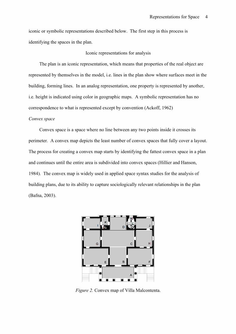
Representations for Space 4
iconic or symbolic representations described below. The first step in this process is
identifying the spaces in the plan.
Iconic representations for analysis
The plan is an iconic representation, which means that properties of the real object are
represented by themselves in the model, i.e. lines in the plan show where surfaces meet in the
building, forming lines. In an analog representation, one property is represented by another,
i.e. height is indicated using color in geographic maps. A symbolic representation has no
correspondence to what is represented except by convention (Ackoff, 1962)
Convex space
Convex space is a space where no line between any two points inside it crosses its
perimeter. A convex map depicts the least number of convex spaces that fully cover a layout.
The process for creating a convex map starts by identifying the fattest convex space in a plan
and continues until the entire area is subdivided into convex spaces (Hillier and Hanson,
1984). The convex map is widely used in applied space syntax studies for the analysis of
building plans, due to its ability to capture sociologically relevant relationships in the plan
(Bafna, 2003).
Figure 2. Convex map of Villa Malcontenta.

Representations for Space 5
The convex map of Villa Malcontenta is shown in figure 2, where each convex space is
labeled with a letter and indicated by a filled rectangle. There are some uncovered areas in
the doorways which are disregarded, because they are not large enough on their own to be
entered and used by humans. The first convex space identified is C, and the rest follows in a
straightforward way.
Axial space
Axial space is a straight line or sight line, possible to follow on foot. An axial map is a
discrete mapping overlaid on top of the convex map. It consists of the least number of axial
lines covering all convex spaces of a layout and their connections. The procedure for
generating an axial map is iterative and starts with the longest line that passes through at least
one permeable threshold between two adjacent convex spaces and repeats this until all the
permeable thresholds between all adjacent convex spaces have been crossed (Batty & Rana,
2004). All the points inside a space should be visible from the axial line through that space.
The resulting network of intersecting straight lines is the axial map. The axial map of Villa
Malcontenta superimposed on the convex map is shown in figure 3. The axial lines are
numbered in the order they are identified.
Figure 3. Axial map of Villa Malcontenta.
Representations for Space 6
The axial space is a suitable abstraction for describing and analyzing the street network
in urban areas, where line of sight is a significant unifying device, and the number of turns on
a route are more crucial to spatial experience than distance covered. Movement, options for
mobility, potential for unplanned encounters are captured by the alignments of the constituent
convex spaces of axial maps (Bafna, 2003).
Isovist space
Convex and axial spaces show space-to-space permeability. Isovist space makes
explicit the relation of visibility. An isovist is the nonconvex space visible around a
viewpoint. The viewpoint is defined alternatively as a single point, all points inside a convex
space, inside a diamond shaped area at the center of a convex space, or on an axial line (Batty
& Rana, 2004).
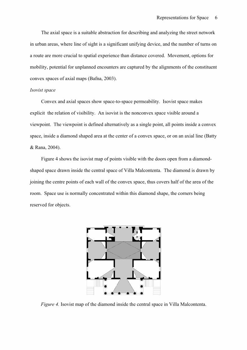
Figure 4 shows the isovist map of points visible with the doors open from a diamond-
shaped space drawn inside the central space of Villa Malcontenta. The diamond is drawn by
joining the centre points of each wall of the convex space, thus covers half of the area of the
room. Space use is normally concentrated within this diamond shape, the corners being
reserved for objects.
Figure 4. Isovist map of the diamond inside the central space in Villa Malcontenta.

Representations for Space 7
Looking at the isovist map in figure 4, we can guess that the central space has a more
powerful visual field than the other convex spaces on the floor. These visibility differences
can form the basis for visual or quantitative and statistical analyses.
Symbolic representations for analysis and synthesis
The iconic representations such as the different types of plans are converted to symbolic
representations for further analysis. One of the most common representations for a spatial
configuration is the graph. Different types of graphs and other representations for qualitative
reasoning are discussed below.
Convex map graph and axial map graph
One of the most common representations for a spatial configuration is the graph. A
graph consists of nodes and edges. Graphs are used for analysis of spatial complexes, as in
space syntax method, and in generation programs for synthesizing layouts. Many different
types of graphs showing different attributes of a layout have been used. Figure 5 shows two
such graphs used in space syntax analysis. The convex map graph on the left is derived from
the convex map shown in figure 2. The nodes of the graph are the convex spaces which have
similar labels as in figure 2. The edges of the graph indicate that it is possible to go directly
from one space to the other.
Figure 5. Convex map graph (left) and axial map graph (right) of Villa Malcontenta.
Representations for Space 8
As with the convex map, the axial map is also easily represented as a graph in which
each axial space is represented by a node and each intersection between two axial spaces as
an edge. The graph at right in figure 5 shows the axial map graph of the axial map in figure 3.
Similar graph can be formed of isovists and overlap relations between them. An isovist map
graph can be formed by taking isovists as nodes and indicating overlapping isovists by links.
The convex map graph takes into account only access and topological features of a
configuration. The premise behind this abstraction is that sociologically relevant aspects of
configured space, such as issues of control and privacy can be captured at the level of
topological description.
Measures of a space, such as connectivity, number of immediate neighbours;
integration, average depth to all other spaces; control value, degree to which a space controls
access to its immediate neighbours considering also the alternative connections available; and
global choice, measure of the flow through a space which depends on how many of the
shortest paths pass through it are based on the information represented in graphs. The above
four measures are called first order measures. Second order measures are formed by
correlating some of these, i.e. the correlation between connectivity and integration, termed
intelligibility.
Measures obtained from the axial map graph has proved useful for the analysis of
pedestrian travel patterns and activities related to such patterns, i.e. the potential for
unplanned encounters, location of services and crime distribution. (Turner, Penn, Hillier,
2005)
Topological descriptions allow researchers a systematic way of disregarding small and
generally sociologically irrelevant geometrical differences, thus enabling several different
layouts to be classified together under a broader typological category (Bafna, 2003).

Representations for Space 9
Adjacency graph
Another type of graph, similar to the convex map and axial map graphs shown in figure
5 above is the adjacency graph. Whereas the convex map and axial map graphs show
existing direct movement and visibility relationships in a plan, the adjacency graph shows all
adjacency relations which make direct movement and visibility relations possible.
An adjacency graph shows spaces by nodes and a boundaries between spaces by edges
connecting the nodes. It can be drawn by replacing each space by a node, and each common
oundary by an edge. Such a plan is called the dual of the plan, as it contains the same
topological information about shapes and their relations as the plan it is derived from
(Kozminski, Kinnen, 1984).
Figure 6. A simplified block plan of Villa Malcontenta and its adjacency graph.
Figure 6 shows a simplified plan of Villa Malcontenta, and its dual. In the plan, walls
are indicated by a single line, a number of the smaller spaces are replaced by two larger
spaces, and the porch, space A in figure 2, is eliminated so that the plan fits inside a
rectangle. Four outside nodes at the north, south east and west are added. We notice that a +
junction in the plan, formed by the walls of four spaces, such as that formed by the spaces I,

Representations for Space 10
K, G, and C results in a four-sided face in the dual. A T junction in the walls where three
spaces meet, for example G, E and C, results in a triangular face in the dual.
Such graphs have been used for generating layouts. When the exterior boundary and all
interior spaces are restricted to be rectangular, we can start with the four external nodes and a
node representing each interior space and add an edge for every required permeability
relation. Then we can add edges in all possible ways until all faces in the dual are triangular
to get all plans satisfying the requirements. This is the opposite of the process of going from
a plan to a convex map graph. We can go from a convex map graph to an adjacency graph,
and from that to a plan.
Wall-representation
Another type of graph used for generating layouts, called a wall representation
considers the adjacency relations between walls and rectangular spaces where a wall is a
maximal continuous straight run of line (Fleming, Baykan, Coyne, Fox, 1992). It records all
the walls and the sequence of rectangles bordering the wall from north and south or east and
west. This type of graph is represented by a string of characters, and generation proceeds by
inserting a new space in all possible locations by operations on the string.
{<1,(N),(W,I,K,D,L,J,E)>,<1,(I,K,D,L,J),(G,C,H)>,<1,(G,C,H)(E,B,F)>,<1,(W,E,B,F,E),(S)>,<-1,(W),(I,G,E)>,<-1,(I,G),(K,C)>,<-1,(K),(D)>,<-1,(E),(B)>,<-1,(D),(L)>,<-1,(B),(F)>,<-1,(L,C),(J,H)>,<-1,(J,H,F),(E)>}
Figure 7. Wall representation of the block plan of Villa Malcontenta shown in figure 6.
Figure 7 shows the block plan of Villa Malcontenta given in figure 6 in wall-
representation format. The wall-representation of the whole plan is enclosed in braces {}.
Walls are ordered from north to south and west to east. Walls are identified by enclosing
brackets < > ; horizontal walls are signified by 1 and vertical walls by -1. The rectangles
Representations for Space 11
north/west and south/east of a horizontal/vertical wall are enclosed in parentheses ()
(Steadman 1983). The northernmost wall in the block plan is bordered by N at north, and by
I, K, D, L and J at south as shown in figures 6 and 7.
Other types of graphs, showing different combinations of space, line and point
adjacencies, are possible. Each type of graph has its own rules of consistency and well-
formedness. A graph is an abstract mathematical representation. It can be drawn on a piece
of paper, possibly in different ways called embedings; and represented symbolically by a list
or an array or a string in a computer or on a piece of paper.
Region connection calculus
The following three representations, region connection calculus, interval algebra and
rectangle algebra are qualitative reasoning methods and are similar with respect to their
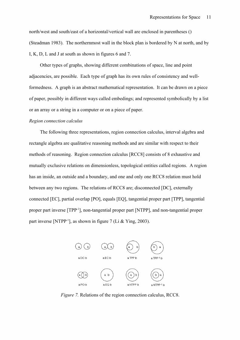
methods of reasoning. Region connection calculus [RCC8] consists of 8 exhaustive and
mutually exclusive relations on dimensionless, topological entities called regions. A region
has an inside, an outside and a boundary, and one and only one RCC8 relation must hold
between any two regions. The relations of RCC8 are; disconnected [DC], externally
connected [EC], partial overlap [PO], equals [EQ], tangential proper part [TPP], tangential
proper part inverse [TPP-1], non-tangential proper part [NTPP], and non-tangential proper
part inverse [NTPP-1], as shown in figure 7 (Li & Ying, 2003).
Figure 7. Relations of the region connection calculus, RCC8.

Representations for Space 12
Reasoning is carried out by composition, which finds the possible relations between
two regions A and C by composing the relations between A and B and B and C. For
example, (A EC B)○(B NTTP C)→(A {PO TTP NTPP} C). This is achieved using a
transitivity table, which is an 8x8 table that shows the composition of every combination of
relations. The relations between every pair of regions need to be represented explicitly,
which can be done using a triangular matrix such as shown in figure 10. Initially all relations
are possible, thus every cell in the matrix contains all 8 relations. The basic operation by
which information is added to the system is by removing some relations from the domain of a
pair of regions. Then by composing the recently changed domain with all others causes a
propagation of the effects, reducing other relations. Any change can lead to a long chain of
propagation, which continues until no more changes are possible. If the domain of a relation
becomes empty, it shows that the relations became inconsistent as a result of the last piece of
information added. This type of reasoning is called constraint propagation. RCC8 relations
can be used for specifying the requirements of a design problem, or as a language for
querying a GIS system.
Interval algebra and rectangle algebra
Interval algebra [IA] is for reasoning about one dimensional entities called intervals. Its
most common application is for reasoning about time intervals. Interval algebra consists of
13 mutually exclusive and exhaustive relations, shown in figure 8. Direction is important in
defining these relations, as before is distinct from after, which are inverse, such that x is
before y and y is after x, as shown in the top line of figure 8 (Allen, 1983).

Representations for Space 13
Figure 8. Relations of interval algebra.
IA relations are similar to RCC8 relations, with directions added. Before and after
correspond to DC, meets and met-by to EC, equals to EQ, etc. Like RCC8, reasoning is by
constraint propagation and composition by a 13x13 transitivity table.
The significance of IA to space layout is that a 2D form of it can be used for reasoning
about rectangles that are parallel to the axes of a Cartesian coordinate system. The relations
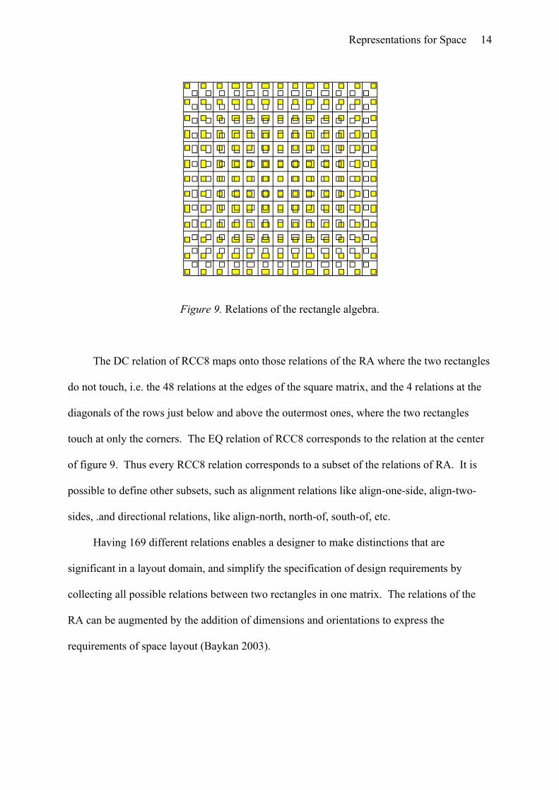
of the rectangle algebra [RA] are derived by the cross product of the 13 relations between two
intervals. This defines 13x13=169 possible mutually exclusive and exhaustive qualitative
relations between two rectangles, as shown in figure 9. Rectangle 1 is shown in grey and
rectangle 2 in white.
Representations for Space 14
Figure 9. Relations of the rectangle algebra.
The DC relation of RCC8 maps onto those relations of the RA where the two rectangles
do not touch, i.e. the 48 relations at the edges of the square matrix, and the 4 relations at the
diagonals of the rows just below and above the outermost ones, where the two rectangles
touch at only the corners. The EQ relation of RCC8 corresponds to the relation at the center
of figure 9. Thus every RCC8 relation corresponds to a subset of the relations of RA. It is
possible to define other subsets, such as alignment relations like align-one-side, align-two-
sides, .and directional relations, like align-north, north-of, south-of, etc.
Having 169 different relations enables a designer to make distinctions that are
significant in a layout domain, and simplify the specification of design requirements by
collecting all possible relations between two rectangles in one matrix. The relations of the
RA can be augmented by the addition of dimensions and orientations to express the
requirements of space layout (Baykan 2003).

Representations for Space 15
Figure 10. RA relations between the spaces of Villa Malcontenta
The RA relations between the spaces of Villa Malcontenta, derived from the layout
shown in figure 6 above, is shown in figure 10. The column labeled Box is the outermost
rectangle, that contains the floor plan. If we specify only the RA relations between the Box
and the other rectangles and between adjacent pairs of rectangles and leave all the others
containing all RA relations in their domains, composition and propagation will be able to
infer the only possible relation that is shown in figure 10.
Orientation
Sometimes we need to take into account the orientations of spaces or objects. Dealing
with rectangles, orientation is either two valued or four valued. When the space is a corridor,
we may want to restrict its width to be 120 cm. Whether this will be in the x or y direction
depends on its orientation. When the object is a refrigerator, its front can face towards N, S,
E or W. These are examples of the absolute orientation of a rectangle. Sometimes we may
need to consider the orientations of rectangles with respect to each other, called relative
orientation.
Representations for Space 16
There are four possibilities for the relative orientation of two objects; parallel,
clockwise-from, opposite, and counter-clockwise-from. It is necessary to specify relative
orientation together with some rectangle relations. We may specify relationships in kitchen
layout, such as the front of the refrigerator should face the use-area, or that refrigerator, sink
and range can be parallel to or facing each other, but not facing in opposite directions.
Reasoning with orientations is another example of qualitative reasoning, similar to RCC8, IA
and RA (Baykan 2003).
Equations
The representations discussed above dealt with qualitative relations in layouts.
Algebraic equations can represent both quantitative and qualitative aspects of rectangular
layouts. Bounded-difference equations can be used to represent RA relations and
dimensional relationships that can be expressed as the distance between two lines.. Linear
equations can express other relationships, such as that the lengths of two spaces are equal, or
that they are centered on the same line, etc. Areas and aspect ratios can be described by non-
linear equations.
Bounded-difference equations
The relations of IA can be expressed by {<, =, >} relations between endpoints of
intervals, and the relations of RA by the same relations between the vertical and horizontal
edges of rectangles.
The difference between two points or lines is shown by a bounded-difference equation
[BNDF] is an equation of the form xi – xj ≤ d. BNDF equations can also represent
dimensional relationships, such as distance, overlap, and dimensions. When the domain of a
BNDF equation is an interval, showing minimum and maximum allowable distance, as in xi –
xj ≤ [dmin, dmax], it can be expressed by two equations in canonical form as follows: xi – xj ≤
dmax and xj – xi ≤ -dmin . These equations can be shown on a matrix, where the first variable in
Representations for Space 17
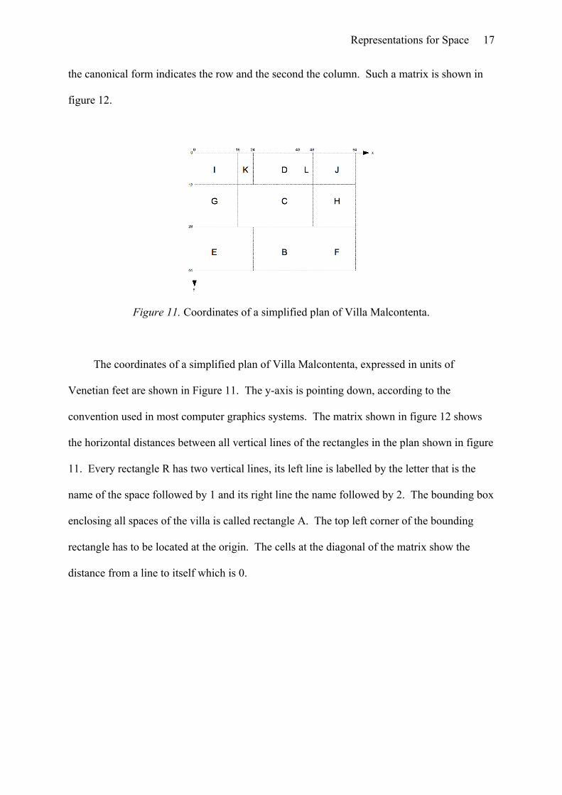
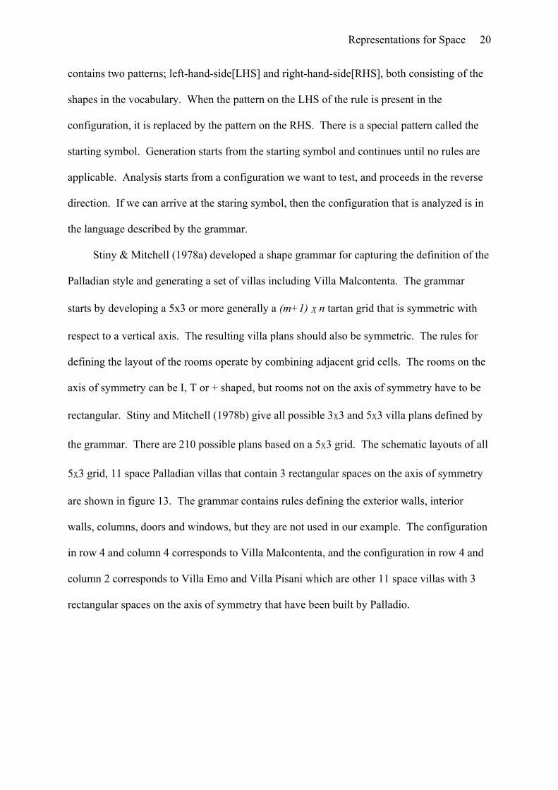
the canonical form indicates the row and the second the column. Such a matrix is shown in
figure 12.
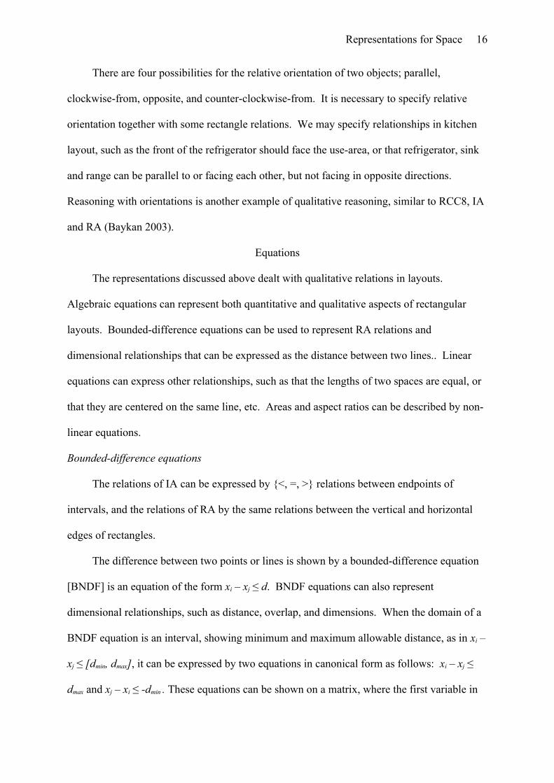
Figure 11. Coordinates of a simplified plan of Villa Malcontenta.
The coordinates of a simplified plan of Villa Malcontenta, expressed in units of
Venetian feet are shown in Figure 11. The y-axis is pointing down, according to the
convention used in most computer graphics systems. The matrix shown in figure 12 shows
the horizontal distances between all vertical lines of the rectangles in the plan shown in figure
11. Every rectangle R has two vertical lines, its left line is labelled by the letter that is the
name of the space followed by 1 and its right line the name followed by 2. The bounding box
enclosing all spaces of the villa is called rectangle A. The top left corner of the bounding
rectangle has to be located at the origin. The cells at the diagonal of the matrix show the
distance from a line to itself which is 0.
Representations for Space 18
Figure 12. Matrix showing horizontal-distances between vertical lines of Villa Malcontenta.
Consistency of bounded-difference constraints can be checked by the Floyd-Warshall
all pairs shortest path algorithm, or if constraints are added one at time, by an incremental
version of the same algorithm (Baykan, 1997). RA and BNDF are both for reasoning about
configurations of rectangles. RA reasoning takes into account only qualitative (topological)
relationships and BNDF quantitative (dimensional) relationships. When topology is
concerned, RA reasoning detects inconsistencies before BNDF does, therefore it is more
complete. But BNDF does not allow any incorrect solutions, thus they are both correct.
Linear equations
Bounded difference equations are a more restricted form of general linear equations and
can be solved by the methods of linear programming [LP]. When we need to express other
relationships such as two dimensions being equal, or two rectangles having the same vertical
center, that cannot be represented by BNDF equations, we can use general linear equations
that may be solved by the methods of linear programming (Dantzig, 1998). Some space
A1 A2 B1 B2 C1 C2 D1 D2 E1 E2 F1 F2 G1 G2 H1 H2 I1 I2 J1 J2 K1 K2 L1 L2
A1 0 64 24 40 16 48 24 40 0 24 40 64 0 16 48 64 0 16 48 64 16 24 40 48
A2 -64 0 -40 -24 -48 -16 -40 -24 -64 -40 -24 0 -64 -48 -16 0 -64 -48 -16 0 -48 -40 -24 -16
B1 -24 40 0 16 -8 24 0 16 -24 0 16 40 -24 -8 24 40 -24 -8 24 40 -8 0 16 24
B2 -40 24 -16 0 -24 8 -16 0 -40 -16 0 24 -40 -24 8 24 -40 -24 8 24 -24 -16 0 8
C1 -16 48 8 24 0 32 8 24 -16 8 24 48 -16 0 32 48 -16 0 32 48 0 8 24 32
C2 -48 16 -24 -8 -32 0 -24 -8 -48 -24 -8 16 -48 -32 0 16 -48 -32 0 16 -32 -24 -8 0
D1 -24 40 0 16 -8 24 0 16 -24 0 16 40 -24 -8 24 40 -24 -8 24 40 -8 0 16 24
D2 -40 24 -16 0 -24 8 -16 0 -40 -16 0 24 -40 -24 8 24 -40 -24 8 24 -24 -16 0 8
E1 0 64 24 40 16 48 24 40 0 24 40 64 0 16 48 64 0 16 48 64 16 24 40 48
E2 -24 40 0 16 -8 24 0 16 -24 0 16 40 -24 -8 24 40 -24 -8 24 40 -8 0 16 24
F1 -40 24 -16 0 -24 8 -16 0 -40 -16 0 24 -40 -24 8 24 -40 -24 8 24 -24 -16 0 8
F2 -64 0 -40 -24 -48 -16 -40 -24 -64 -40 -24 0 -64 -48 -16 0 -64 -48 -16 0 -48 -40 -24 -16
G1 0 64 24 40 16 48 24 40 0 24 40 64 0 16 48 64 0 16 48 64 16 24 40 48
G2 -16 48 8 24 0 32 8 24 -16 8 24 48 -16 0 32 48 -16 0 32 48 0 8 24 32
H1 -48 16 -24 -8 -32 0 -24 -8 -48 -24 -8 16 -48 -32 0 16 -48 -32 0 16 -32 -24 -8 0
H2 -64 0 -40 -24 -48 -16 -40 -24 -64 -40 -24 0 -64 -48 -16 0 -64 -48 -16 0 -48 -40 -24 -16
I1 0 64 24 40 16 48 24 40 0 24 40 64 0 16 48 64 0 16 48 64 16 24 40 48
I2 -16 48 8 24 0 32 8 24 -16 8 24 48 -16 0 32 48 -16 0 32 48 0 8 24 32
J1 -48 16 -24 -8 -32 0 -24 -8 -48 -24 -8 16 -48 -32 0 16 -48 -32 0 16 -32 -24 -8 0
J2 -64 0 -40 -24 -48 -16 -40 -24 -64 -40 -24 0 -64 -48 -16 0 -64 -48 -16 0 -48 -40 -24 -16
K1 -16 48 8 24 0 32 8 24 -16 8 24 48 -16 0 32 48 -16 0 32 48 0 8 24 32
K2 -24 40 0 16 -8 24 0 16 -24 0 16 40 -24 -8 24 40 -24 -8 24 40 -8 0 16 24
L1 -40 24 -16 0 -24 8 -16 0 -40 -16 0 24 -40 -24 8 24 -40 -24 8 24 -24 -16 0 8
L2 -48 16 -24 -8 -32 0 -24 -8 -48 -24 -8 16 -48 -32 0 16 -48 -32 0 16 -32 -24 -8 0

Representations for Space 19
layout programs, such as those given in Mitchell, Steadman, Liggett (1976) and Flemming
(1978), use a two step approach to the generation of layouts. In the first step, topology is
determined. In the second step, linear equations are formed based on the topology and
dimensional constraints and solved by a linear programming package to calculate the
dimensions of the layout.
Non-linear equations
In space layout, we need to consider the areas and aspect ratios of rooms. In Villa
Malcontenta, Palladio used only specific aspect ratios, such as 1:1, 1:2, 1:√2, etc. In most
building codes, there are minimum area requirements for bedrooms and houses. Areas and
aspect ratios require non-linear equations, which can be handled by general non-linear
programming methods or by more specific methods restricted to area and aspect-ratio
calculation which can be much more efficient.
Mixed integer linear or non-linear equations
Integer programming uses integer variables which can take 0 or 1 as values to represent
choices or alternatives. This makes it possible to model different topologial alternatives.
Integer and linear or non-linear variables can be used together to model the topological and
dimensional aspects of a layout problem. The methods for solving such a model are called
mixed integer linear programming [MILP] or mixed integer non-linear programming
[MINLP]. A space layout problem that aims to define the topology as well as the dimensions
of a layout can be formulated as a MILP or a MINLP. There is no guarantee that the
resulting problem can be solved or solved in a reasonable time by an existing solver. If it can
be solved, the result will be only one optimal solution and not a range of alternatives.
Shape grammars
Another formalism for describing, analyzing and synthesizing layouts is a shape
grammar. A shape grammar is defined by a vocabulary of shapes and a set of rules. A rule
Representations for Space 20
contains two patterns; left-hand-side[LHS] and right-hand-side[RHS], both consisting of the
shapes in the vocabulary. When the pattern on the LHS of the rule is present in the
configuration, it is replaced by the pattern on the RHS. There is a special pattern called the
starting symbol. Generation starts from the starting symbol and continues until no rules are
applicable. Analysis starts from a configuration we want to test, and proceeds in the reverse
direction. If we can arrive at the staring symbol, then the configuration that is analyzed is in
the language described by the grammar.
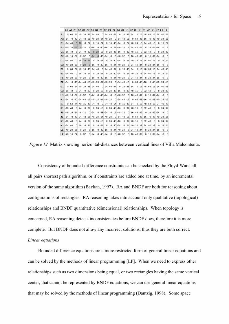
Stiny & Mitchell (1978a) developed a shape grammar for capturing the definition of the
Palladian style and generating a set of villas including Villa Malcontenta. The grammar
starts by developing a 5x3 or more generally a (m+1) x n tartan grid that is symmetric with
respect to a vertical axis. The resulting villa plans should also be symmetric. The rules for
defining the layout of the rooms operate by combining adjacent grid cells. The rooms on the
axis of symmetry can be I, T or + shaped, but rooms not on the axis of symmetry have to be
rectangular. Stiny and Mitchell (1978b) give all possible 3x3 and 5x3 villa plans defined by
the grammar. There are 210 possible plans based on a 5x3 grid. The schematic layouts of all
5x3 grid, 11 space Palladian villas that contain 3 rectangular spaces on the axis of symmetry
are shown in figure 13. The grammar contains rules defining the exterior walls, interior
walls, columns, doors and windows, but they are not used in our example. The configuration
in row 4 and column 4 corresponds to Villa Malcontenta, and the configuration in row 4 and
column 2 corresponds to Villa Emo and Villa Pisani which are other 11 space villas with 3
rectangular spaces on the axis of symmetry that have been built by Palladio.

Representations for Space 21
Figure 13. Some Palladian villas defined by the grammar of Stiny & Mitchell (1978b).
Most grammars have been developed to describe and analyze historical or existing
styles, as defined by a corpus of designs. The rules of the grammar are inferred by analysis
of existing designs and tested by using the rules to generate designs in the corpus as well as
new designs. The clarity of the description is important. It is also possible to develop
original grammars to define new styles.
Grammars are used widely in space layout. The basic idea is very general and intuitive,
but it is hard to automate a general mechanism for operating with shape grammars. Shape
grammars are symbolic rather than iconic representations. This makes it possible to
implement grammars as computer programs, but the symbolic to iconic correspondence is
different for each grammar.
Discussion
The representations discussed above are by no means exhaustive. Some that have been
omitted are polygonal representations as used in geographic information systems [GIS], grids
as used in the quadratic assignment formulation [QAP] (Liggett; 2000); and pixels.

Representations for Space 22
It is possible to discuss representations with respect to what they express, whether they
are iconic or symbolic, qualitative or quantitative, procedural or declarative, and the
correctness, completeness and complexity of the reasoning mechanisms that are applicable.
Representations that use constraint satisfaction as a reasoning mechanism, such as
RCC8, RA and BNDF are declarative, that is we are not concerned with the order of
application of the constraints. Doing it in a particular order may be more efficient that
another, but both give the same result. Shape grammars are procedural. They also define the
application order of the rules. In a constraint-based generation process, a list of spaces and
the constraints on them are given. In a grammatical approach, we start with a single symbol
and add patterns or modify them in some order.Grammars may be more intuitive in that
respect.
Analysis starts with an existing spatial structure and abstracts it using one of the
representations discussed above to get to the relevant aspects. Synthesis starts with some
abstraction that embodies the requirements and adds more information until it defines a
spatial structure in sufficient detail for it to be realized.
Conclusion
Every representation makes some features explicit and hides or omits others. The
representations discussed above also give an indication of issues that are considered in the
analysis and synthesis of layouts by the features they consider. Based on what is explicit, a
representation makes some operations easy and others very hard or impossible. Analysis
goes from concrete to abstract representations by omitting details and synthesis proceeds in
the other direction, adding more information and details.

Representations for Space 23
References
Ackoff, R L. (1962). Scientific Method, NewYork: John Wiley & Sons.
Allen, J. F. (1983). Maintaining Knowledge about Temporal Intervals, Communications of
the ACM, 26, 832-843.
Bafna, S. ( 2003). Space Syntax A Brief Introduction to Its Logic and Analytical Techniques,
Environment and Behavior, 35, 17–29.
Batty, M., Rana, S. (2004). The automatic definition and generation of axial lines and axial
maps, Environment and Planning B: Planning and Design, 31, 615–640.
Baykan, C. A., Pultar, M. (1995). “Structure of space activity relations in houses”. Presented
at Eindhoven, Holland: IAPS, Spatial Analysis in Environment-Behavior Studies
Conference. Retrieved February 12, 2009, from
http://www.metu.edu.tr/~baykan/publications-pdf/baykan-iaps95.pdf
Baykan, C. A., Fox, M. S. (1997). Spatial Synthesis by Disjunctive Constraint Satisfaction,
Artificial Intelligence for Engineering Design, Analysis and Manufacturing [AI
EDAM], 11, 245–262.
Baykan, C. A. (2003). Spatial Relations and Architectural Plans: Layout problems and a
language for their design requirements in B. Tuncer, Ş S. Özsarıyıldız, S. Sarıyıldız
(Eds.) E-Activities in Design and Design Education. (edited by). Paris: Europia
Productions, 137–146.
Dantzig, G. B. (1998). Linear Programming and Extensions, Princeton, NJ: Princeton
University Press. (11th printing).
Flemming, U., Baykan,C. A., Coyne,R., Fox, M. S. (1992). Hierarchical Generate and Test
vs. Constraint-Directed Search, A Comparison in the Context of Layout Synthesis. In
J.S. Gero (Ed.), Artificial Intelligence in Design '92 (pp. 817–838). Dordrecht: Kluwer
Academic Publishers.

Representations for Space 24
Flemming, U. (1978). Wall representations of rectangular dissections and their use in
automated space allocation. Environment and Planning B 5, 215–232 .
Habraken, N. J. (1998). The structure of the ordinary: form and control in the built
environment. Cambridge, Massachusetts: The MIT Press.
Hillier, B., Hanson, J. (1984). The social logic of space. Cambridge, UK: Cambridge
University Press.
Kozminski K., Kinnen E. (1984) An algorithm for finding a rectangular dual of a planar
graph for use in area planning for VLSI integrated circuits. Proceedings of the 21st
Design Automation Conference, Albuquerque, New Mexico, United States.
Li, S., Ying, M. (2003). Region Connection Calculus: Its models and composition table,
Artificial Intelligence, 145, 121–146.
Liggett, R. S. (2000). Automated facilities layout: past, present and future, Automation in
Construction, 9, 197–215.
Mitchell, W. J., Steadman, J. P., Liggett R. S. (1976). Synthesis and optimization of small
rectangular floor plans, Environment and Planning B: Planning and Design, 3, 37–70.
Palladio, A. (1997). The Four Books on Architecture, Cambridge, Massachusetts: The MIT
Press.
Steadman J P. (1983). Architectural morphology: an introduction to the geometry of building
plans, Pion.
Stiny, G., Mitchell, W. J. (1978a). The Palladian grammar, Environment and Planning B, 5,
5–18.
Stiny, G., Mitchell, W. J. (1978b). Counting Palladian plans, Environment and Planning B, 5,
189–198.
Goldschmidt Gabriela, Porter William L. (2004). “Design representation”. London, NY:
Springer, p. 203.