Representation of Digital Maps

Viktor Veis 21.12.2001 University of Joensuu Department of Computer Science Master’s Thesis

i

Table of contents 1. Introduction 1 2. Digital map formats 4

2.1. Raster formats 5 2.1.1. Single image map 5 2.1.2. Layer conception 6

2.2. Vector formats 8

2.2.1. Point 8 2.2.2. Polyline 8 2.2.3. Polygon 8 2.2.4. Rectangle 9 2.2.5. Circle 9 2.2.6. Arc 10 2.2.7. Bezier curve 10 2.2.8. Primitive attributes 10 2.2.9. SVF (Simple Vector Format) 11 2.2.10. ArcShape format 11

2.3. Conversion of digital maps to another format 14

3. From vector to raster 17

3.1. Goals of the rasterization 18

3.2. Basic ideas of rasterization 20 3.2.1. Format independent vector structure 21 3.2.2. Project file 23

3.3. Graphics library 24

3.3.1. Scale problem 24 3.3.2. Line drawing algorithm 25 3.3.3. Area filling algorithm 25 3.3.4. Polygon filling algorithm 27 3.3.5. Circle drawing algorithm 31 3.3.6. Arc drawing algorithm 32 3.3.7. Text output using Hershey vector font 34 3.3.8. Another image drawing algorithm 37 3.3.9. Bezier curve algorithm 37 3.3.10. Conclusions 38

3.4. ArcShape design 39

3.4.1. File design 39 3.4.2. Line styles and fill attributes 40 3.4.3. Coordinate conversion 42

ii

4. Map compression 44

4.1. Compression methods 45 4.1.1. Arithmetic coding 48 4.1.2. JBIG 49 4.1.3. LZW coding 51

4.2. Compression of vector maps 54

4.2.1. Random algorithm 54 4.2.2. Douglas-Peucker algorithm 54 4.2.3. Pipe algorithm 56 4.2.4. Cones intersection algorithm 58

4.3. Compression of raster maps 59

4.3.1. Dynamic map handling 59 4.3.2. MISS map as a hierarchical structure 60 4.3.3. Dynamic and direct access 61 4.3.4. Continue index table 62 4.3.5. MISS file structure 63

5. Experiments 66 6. Conclusions 71 References 76

iii

List of Figures 1.1 Example of the legend 1 1.2 The latitude-longitude definition 2 1.3 Different map scales 2 2.1 Color, grayscale and binary formats of the same raster image 5 2.2 The map and its layer separation 6 2.3 Step by step reconstruction of original image in the layer conception 6 2.4 Example of a polygon 19 2.5 Rectangle primitive 19 2.6 Circle primitive 19 2.7 Arc primitive 10 2.8 Bezier curve 10 2.9 A polyline primitive is drawn with different width and styles 11 2.10 Dividing NLS map by four parts 12 2.11 General scheme of conversion between different digital map formats 14 3.1 Raster and vector zooming 19 3.2 Basic scheme of rasterization 20 3.3 A scheme of using format independent vector structure 21 3.4 All cases of direction of coming and leaving a horizontal line in the polygon border 27 3.5 A polygon with a hole processed using start-end technique 28 3.6 Polygon is filled using start-end technique 29 3.7 Example of the polygon, where two borders cross one pixel 29 3.8 A polygon with associated values 29 3.9 A circle on the grid with a part drawing by Bresenham algorithm 32 3.10 Dividing a plane by eight parts 33 3.11 Three basic cases, when the part approach is working 33 3.12 Character “A” with coordinate pairs 35 3.13 Structure of the array LAYERS 39 3.14 A scheme of using the topological sign library 41 3.15 A scheme of FILL_STYLES array 42 4.1 A binary image with one black pixel 45 4.2 A binary image with a set of black pixels 47 4.3 Interval [0,1] is divided into 8 parts, thus each having the length of 2-3=0.125 48 4.4 JBIG sequential model templates 49 4.5 Compression model without context 50 4.6 Sample compression ratios for context-based compression 51 4.7 LZW dictionary in tree representation 53 4.8 Douglas-Peucker algorithm 55 4.9 Pipe algorithm 57 4.10 Dynamic map handling 60 4.11 Image blocks numbering 60 4.12 An overall structure of MISS map 61 4.13 A scheme of compression one layer 62 4.14 A structure of the first block of the continue index table 63 4.15 A structure of the MISS file 64 5.1 Example of the project file 68

iv

List of Tables 3.1 Fields of the format independent vector structure 22 3.2 Fields of PRIMITIVE structure 23 3.3 Structure of the project file 23 3.4 Criterion of marking start and end pixels 28 4.1 Compression model without context 50 4.2 Compression model with two pixels in the context 51 4.3 An example of LZW coding 52 4.4 An example of LZW decoding 53 4.5 MISS file header 64 4.6 MISS page header 64 4.7 MISS layer header 65 4.8 MISS block header 65 5.1 Statistics of map conversion from ArcShape format to MISS file 68 5.2 ArcShape map conversion in bytes 69 5.3 Raster map conversion statistic 69 6.1 Comparison of map formats 72 6.2 Relative measuring of the quality of the map formats 74

v

Abstract

Digital maps can be stored and distributed electronically using compressed raster image formats. We will look into the details of maps, their digital representation, their abilities and how they can be efficiently used. We review the ways of representation of raster maps, layer conception and pay attention to the vector formats, especially to the ArcShape and SVF formats. Also, the scheme of conversion between different digital map formats will be considered. We consider the rasterization problem in detail. For this purpose we have collected and developed a set of tools tailored for transforming vector primitives to raster form. The image in raster form is a good source for various methods of compression. Some of them are studied and the new Map Image Storage System (MISS) is introduced. The main objective of the proposed storage system is to provide map images for real-time applications that use portable devices with low memory and computing resources. Compact storage size is achieved by dividing the image into binary layers, which are then compressed using context-based method. The storage system allows dividing the image by blocks, storing them in compressed format and providing direct access to the compressed file. Empirical results show that the MISS format achieves better compression than other well-known methods, such as GIF and PNG.

1

1 Introduction In general, a map is a picture that represents some area in the world. However, it is not a

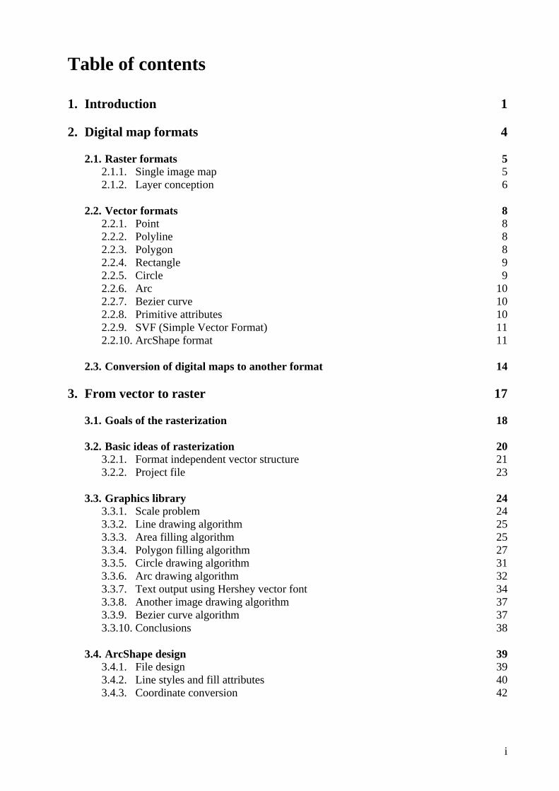
photo from a satellite, but the picture, which contains information about the area using some legend. We can think about a map as about a set of geographical objects such as roads, buildings, rivers, lakes, seas, etc. Each object has appropriate code sign, color or another feature of drawing style. This appropriation is a cartography term and called a legend. Figure 1.1 shows a piece of the map with the legend explanation. Area Main road Elevation line Small road Swamp Path Lake Buildings Name of the lake

Figure 1.1: Example of the legend.

Next, we should have a method for binding a map to the region it represents. First of all, the Earth has a highly irregular and constantly changing surface, but a region of the Earth can be approximated by the piece of sphere. A lot of map systems were developed to represent a piece of sphere on the plane. Further, we will not concentrate our attention on these systems and assume that all maps are situated on the plane and each plane point has its own coordinate.

Coordinate is a pair of parameters that allows binding an abstract map point with the

point in the real world. There are many coordinate systems, but the most common system is geo spherical system [5], which uses two parameters: Latitude and Longitude. The Latitude is an angle in the vertical direction from equator to the point; diapason of the latitude is from –90 (south pole) to +90 (north pole) degrees. The Longitude is an angle in the horizontal direction from the Greenwich meridian to the point; diapason of the longitude is from 0 to 180 degrees east longitude and from 0 to 180 degrees west longitude. Figure 1.2 demonstrates the latitude-longitude definition. Thus, a pair (latitude, longitude) is sufficient to define any position on the surface of globe.

Coordinates of two diagonal map points are enough for binding a map to the appropriate

region. The sufficient information for binding a map we will call sufficient geographical information. Sometimes a map is covered by a coordinate grid that allows finding an estimated coordinate of any point of the map at first sign.

2

Figure 1.2: The latitude-longitude definition.

Another important map parameter is a map scale. The map scale is a ratio of the distance between two points of the geographical world to the distance between appropriate points in the map. This parameter is the same for the entire map because map scaling is linear. If coordinates of two diagonal points and a map size are known, we can calculate the map scale. The same is in the opposite direction: a coordinate of the corner map point and the map scale are sufficient geographical information for location any point in the map.

Maps with different scale are used for different goals. For example, maps with big scale

allow viewing big regions in one map. Such maps can be used for planning a trip. Maps with small scale contain many map details. Such maps are used for finding specified object and for orientation. Figure 1.3 shows two maps of the same place with different scale. The area represented by the right map is marked by dashed rectangle on the left map. The geographical areas are the same but images are totally different. In other words, the right map can not be made by zooming a subimage from the left map. This happens because the map information depends on the map scale.

1 : 80 000 1 : 20 000

Figure 1.3: Different map scales.

World Geographical point Greenwich Longitude Equator Latitude

3

Further, we will understand a map as a visual information about some area with the legend, the geographical information and the scale.

A digital map is a map that is stored, browsed and processed by computer. Some years ago, there were no computers and maps were stored just on the paper. Papers became old, took a lot of place and were difficult to create. Computers allow to process images, to copy and to send them easily. Thus, computers help to solve paper map problems and add new possibilities to the map technologies. Digital map processing allows:

• Storing a huge set of maps in compact and mobile device, such as laptop, Pocket PC, even mobile phone.

• Compress maps using image compression technologies. • Storing map databases on servers. • Transfer maps using network technologies. • Create well-design and comfortable interface for map browsing • Provide a map-based service.

Finally, we can specify a goal of using digital maps: provide service that allows a customer to get to his mobile device a map of the surround area with the necessary resolution and customer’s location on the map. This service must take minimum memory and transfer resources.

In the digital images, the universal distance measure is a pixel. The linear size of the

same image can be different depending on the computer configuration. Thus, a scale is not used when dealing with digital maps. We will use another parameter, which is called a map resolution. The map resolution gives the number of meters in one pixel. A digital map can be considered as a set of the following parameters:

1. image, 2. resolution, 3. geographical information, 4. legend.

Dealing with digital map formats, we should pay attention to follow points.

1. Browsing: very important to have easy and fast possibility to browse a map. 2. Map scaling: any format must support multiple scales of the map. 3. Compression: a map should take as small space as possible. 4. Map transfer: the map format ought to support easy and fast transferring via

communication networks. 5. File format: the format is supposed to be understandable and must have a possibility for

further improvements (e.g. add new compression methods). In the following, we use these criteria for comparing different map formats.

4

Chapter 2 Digital map formats

This chapter defines digital map, reviews raster map formats and vector map formats and shows the ways of conversion between them. The chapter contains many definitions, which will be used below. The first part considers conception of digital maps, shows difference between a digital map and a digital image and gives a scheme of map creation process. The second part gives raster map conception, a single image map and a map with layer separation. The third part gives definition of vector map. It describes graphics primitives and their implementation in SVF and ArcShape formats. The fourth part gives general picture of map formats and conversion between them.

5

2.1 Raster formats

Raster digital map stores visual information as a raster image or as a set of raster images. A raster image is a way of storing digital graphics. Raster images are classified depends on representation of the color of the pixel. We are interested of four types of raster images:

1. True color images: each color is a triple of color components (RGB, YUV or HSI) [10]. Usually, one color component is stored in one byte. Thus, a color image uses three bytes for storing a color of one pixel.

2. Palette images: if an image consists of a little number of colors, we can use a palette to improve its structure. Palette is a color dictionary, which associates each color with some number. Using a palette, a color of the pixel can takes one byte or less space. Palette can be standard or specified for the image. In the second case, the palette should be stored with the image. GIF [16] is one of the most effective formats for palette images.

3. Grayscale images: a color in these images is a gradation between white and black. Thus, a pixel color is one value, which is the pixel brightness. Typically, brightness is stored in one byte. Therefore, a pixel color takes one byte in grayscale images.

4. Binary images: this is an image with black and white colors. The pixel color is stored using one bit (1=black, 0=white).

The types in the list can be converted from top to bottom with losing color information

and decreasing of the space for storing the image. Conversion from bottom to top is impossible without additional information. In the Figure 2.1, there are examples of color, grayscale and binary map images generated from Figure 1.3. It is easy to see that color information is decreased from left to right. Color image Grayscale image Binary image

Figure 2.1: Color, grayscale and binary format of the same raster image. 2.1.1 Single image map

There are two basic approaches for raster maps. The first one stores visual information of the area with predefined scale as one color image with a limited number of colors. This is very simple map format. We have one color image and the geographical information in the separate file. The map resolution can be easily calculated from the image size and the geographical information. The format allows showing a map and locating points on them. Location means finding coordinates of a point on the image and marking a point with specified coordinates on the image. Typically, image formats for this map format are PPM [16], GIF [16] and PNG [16].

6

2.1.2 Layer conception

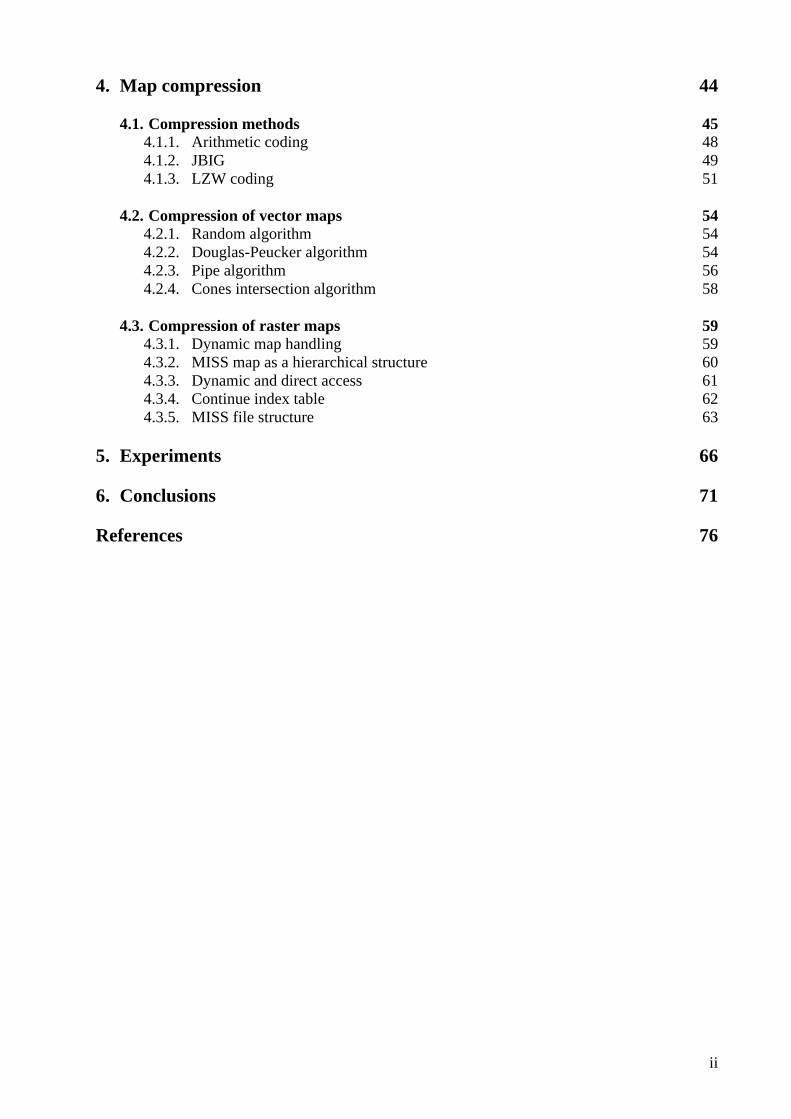
The second approach for raster maps is layer separation. An image with few colors can be easily converted to the set of binary images. Each binary image represents one color from the original image. We will call a binary file from such set with color information as a color layer. Example of the color image and appropriate set of layers are shown in the Figure 2.2. Notice that all binary images have the same size as the original image.

Original image

Layer 1 Layer 2 Layer 3 Layer 4 Layer 5 Blue Yellow Brown Black Red Water Fields Elevation lines Basic Property

Figure 2.2: The map and its layer separation.

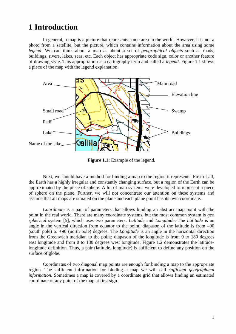
A set of layers is not enough for reconstructing original image. We also require information about background color. Background color in layer conception is the default color of the image. The background color in the Figure 2.2 is white. If the layers cover the entire image, the background color is taken as a color of the biggest layer and this layer is removed from the layer set. Another information we need to reconstruct the image is the order of layers. In the Figure 2.2, the layer order is shown from left to right. The reconstruction process consists of two stages:

1. Fill the image with background color. 2. Draw layers according to the layer order. Black pixels from each layer are drawn using

the appropriate color; white pixels are skipped.

Figure 2.3 shows image reconstruction process step by step.

Figure 2.3: Step by step reconstruction of original image in the layer conception.

7

Using layer approach, we can use binary compression methods and provide layer-by-layer map browsing. Sometimes, user would like to view not all objects on the map, but some logical part of them. This can be done using layer-by-layer browsing.

Let us consider the layer 4, the basic layer. The color of the layer is black, but logical

information in the layer is different. The black layer includes name of the lake, roads, border of fields, etc. This means that all these different objects can be shown in the same time or not shown at all. This is not convenient. A color layer can be divided into logical layers for solve the problem. Unfortunately, the algorithm for this separation does not exist because computer has just color information. Logical separation should be done by human. This makes logical separation difficult and time-required operation. Because of this, the logical separation is not used often in the case of raster maps.

Finally, the layer-separated map format consists of the follow information:

1. Geographical information, 2. Background color, 3. Map resolution, 4. Set of layers (binary images) in order format, 5. Specified color for each layer.

8

2.2 Vector formats

Vector digital map is a digital map, which stores visual and geographical information using vector graphics [25]. In contrast to raster graphics, vector graphics is stored not as an image, but as a set of graphical primitives. Here is the list of the most common primitives:

1. Point 2. Polyline 3. Polygon 4. Rectangle 5. Circle 6. Arc 7. Bezier curve

A primitive is stored using basic values. Basic values are defined for each primitive

separately. In general, basic values are sufficient information for describing the primitive position and the primitive shape. For example, basic values for a point are its coordinates (x,y). The image size in vector graphics is not a parameter of the image. Scaling is doing while drawing the image. Therefore, the point coordinates are relative values. This means that the point coordinates give a point position relatively other shapes in the image. Because of this, real coordinates (Latitude, Longitude or other coordinate system) are used as basic values in vector maps. This approach allows storing geographical information inside the image and providing scaling with very good quality.

Let us consider each primitive in more detailed and look how geographical objects can be

represented using these primitives. Then, we continue with the two common vector map standards: ArcShape and Simple Vector Format (SVF). 2.2.1 Point

The basic values of a point are its coordinates, as was mentioned above. The point primitive can be used for specifying such geographical objects as topological signs or other separated geographical objects, which have predefined shape. For example, the point primitive is also used for placing a text object. 2.2.2 Polyline

Polyline is specified using the number of points n and an array of the coordinates (x[n],y[n]). Roads, paths, channels and other extensive geographical objects with constant width are represented by polylines. 2.2.3 Polygon

The basic values for polygon are the same as for polyline. The basic difference from polyline is that the first point and the last polygon point are the same. The second difference is that polygon border do not cross itself. Thus, a polygon is an area on the plane and can be filled. Filled polygons represent geographical areas such as lakes, rivers with non-standard width, fields, buildings, etc.

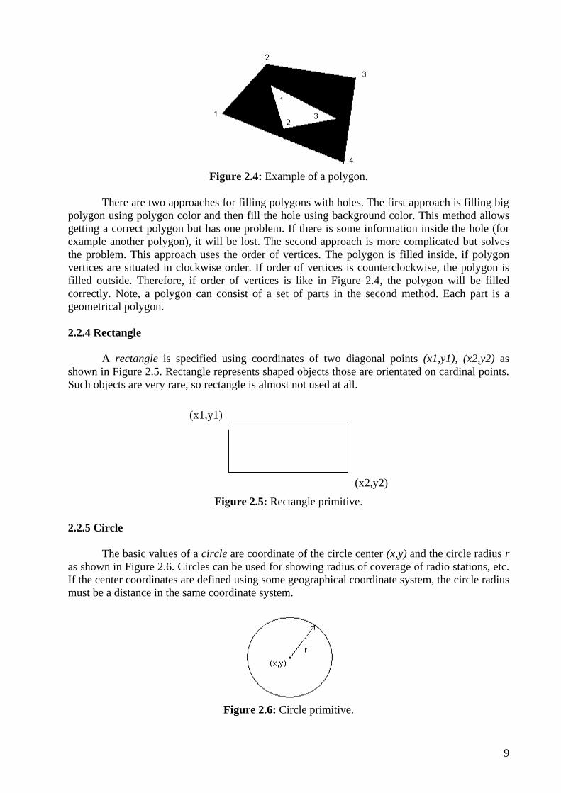
There is one interesting moment of polygon filling. Let us assume that we need to fill a

polygon with a hole as shown in Figure 2.4.

9

Figure 2.4: Example of a polygon.

There are two approaches for filling polygons with holes. The first approach is filling big polygon using polygon color and then fill the hole using background color. This method allows getting a correct polygon but has one problem. If there is some information inside the hole (for example another polygon), it will be lost. The second approach is more complicated but solves the problem. This approach uses the order of vertices. The polygon is filled inside, if polygon vertices are situated in clockwise order. If order of vertices is counterclockwise, the polygon is filled outside. Therefore, if order of vertices is like in Figure 2.4, the polygon will be filled correctly. Note, a polygon can consist of a set of parts in the second method. Each part is a geometrical polygon. 2.2.4 Rectangle

A rectangle is specified using coordinates of two diagonal points (x1,y1), (x2,y2) as shown in Figure 2.5. Rectangle represents shaped objects those are orientated on cardinal points. Such objects are very rare, so rectangle is almost not used at all.

Figure 2.5: Rectangle primitive. 2.2.5 Circle

The basic values of a circle are coordinate of the circle center (x,y) and the circle radius r as shown in Figure 2.6. Circles can be used for showing radius of coverage of radio stations, etc. If the center coordinates are defined using some geographical coordinate system, the circle radius must be a distance in the same coordinate system.

Figure 2.6: Circle primitive.

(x1,y1)

(x2,y2)

10

2.2.6 Arc

An arc is specified using coordinates of the center (x,y), the radius r and the two bounded angles: start angle and end angle. Figure 2.7 demonstrates arc primitive. The arc primitive can represent any ArcShape on the map.

Figure 2.7: Arc primitive. 2.2.7 Bezier curve

Bezier curve is specified using four points. Therefore, the basic values for Bezier primitive are four coordinate pairs. With four points, we can represent a smooth curve with constant width. Figure 2.8 demonstrates a Bezier curve. Points 3210 ,,, PPPP are the basic points.

Using them, we can build control points 21

20 , PP , which specify the tangent. The curve is built

using the two end points 30 , PP and the tangent. Detailed information about Bezier curves can be found in [21].

Figure 2.8: Bezier curve. 2.2.8 Primitive attributes

It is easy to see, that primitive is defined by shape and position of a geographical object. A set of primitives is a scheme of the image. This information is not enough for drawing the image. For drawing a primitive, we must know such primitive’s attributes as color, width, line style, fill style, etc. The list of attributes depends on the primitive type and the type of the geographical object, which the primitive represents. For example, if a primitive represents the road on the map it should have two attributes for drawing: width and line style (solid, dash, dot, etc.). Figure 2.9 shows one primitive drawn using different width and styles.

Thus, a vector map consists of a set of primitives and their attributes. Geographical

information is stored inside primitives; resolution is a parameter of visualization. One vector map

11

of some region covers all scales. This is the main difference between raster and vector maps. Let us now concentrate on two vector map formats: SVF format and ArcShape format. They use different approaches for storing primitive attributes. Width = 1 Width = 3 Width = 1 Style= SOLID Style = SOLID Style = DASH

Figure 2.9: A polyline primitive is drawn with different width and style. 2.2.9 Simple Vector Format (SVF)

SVF [23] uses one file for storing the entire map of some region. Primitive attributes are stored with the primitive. SVF format is based on the tag language and it is supported by Internet Explorer. A special plug-in [23] have to be installed for browsing SVF files. There is no difference between SVF image and SVF map.

SVF map uses polygons with filling holes with background color. This is a drawback of

the format because of loss of the information inside the hole. The advantages of SVF are the simplicity and clarity of the format. Visualization of SVF map is not difficult if software environment supports visualization of graphical primitives. 2.2.10 ArcShape vector format

ArcShape format [6] is more complicated than SVF. It was developed by ESRI [25] for advanced map processing. It supports three types of primitives: Point, Polyline and Polygon. These primitives are enough for representation any map. Primitives could have additional parameters such as Z coordinate (altitude) and a measure. Measure is a value associated with the primitive (for example, the number of road). We will not consider these parameters because they are used only in some special cases. Full technical description of ArcShape format is in [6]. We just mention that ArcShape format uses ordered vertices for filling a polygon.

ArcShape image consists of the set of shapefiles. Each shapefile stores primitives of one

specified type (points, polylines or polygons). A shapefile consists of three files with the same names and different filename extensions:

1. Main file: this file contains all primitives as a set of vector coordinates. There are no primitive attributes in this file. The main file has a filename extension SHP.

2. Database file: primitive attributes are stored in database file with one record per primitive. The one-to-one relationship between geometry and attributes is based on record number. Attribute records in the database file must be in the same order as primitives in the main file. Such structure leads the same attribute pattern for all primitives in one shapefile. The database record fields are not specified. They depend on the concrete ArcShape system. The database file has a filename extension DBF.

3. Index file: this file contains the offsets of the corresponding main file primitives from the beginning of the main file. It is used for providing direct access to the main file. The index file has a filename extension SHX.

12

In other words, ArcShape format separates primitives and their attributes. Moreover, the attribute pattern is specified outside the format depends on the ArcShape implementation. All these features make dealing with ArcShape format not easy. ArcShape software must be oriented to the specified ArcShape map system.

Let us consider ArcShape map database standard in the National Land Survey (NLS) of

Finland [18]. A map consists of a set of logical layers. Each logical layer is a set of four shapefiles (points, polylines, polygons and text). Shapefile belongs to some logical layer and has some primitive type depending on the main file name. The main file in NLS map has the pattern name ?xxxxxx??.shp. The sequence xxxxxx specifies a number of the map and is a constant for all files from one map, for example 431204. The first character of the name defines a logical layer that the shapefile belongs to. The following list shows all possible values of the first character:

• j — administration information, • l — communication objects, • m — areas (lakes, swamps, fields), • n — water, • r — buildings, • k — elevation lines, • s — conservations.

The character after the map number means the part of the ArcShape image. One

ArcShape image consists of four parts; each part is represented by separate shapefile. The image separation is shown in the Figure 2.10. The characters in the boxes are the character after map number in the file name.

Figure 2.10: Dividing NLS map by four parts. The last character gives information of the shapefile type:

• t — text • s — points • v — lines • p — polygons

The text type is actually a point type but there are some reasons for separate these types.

For example, the shapefile with the name m431204Bp contains polygon primitives from top left part (part B) of the areas layer.

Let us consider database file structure in NLS map. The database records have four

important fields: 1. RYHMA. The code of the shapefile. It is the same for different parts of the image but

unique for logical layer and primitive type.

A

B D

C

13

2. LUOKKA. The code of the geographical object represented by the primitive. The code is unique for all geographical objects and is used for specifying primitive attributes.

3. TEKSTI. Text primitives use this text string for output in the map. 4. SUUNTA. This field contains information about a primitive direction. For example,

arrows and text always have an output direction.

As we see, the database file has no information about color, line style and other important primitive attributes. These attributes are stored in legend files. Legend files have a filename extension AVL and allows getting attributes via LUOKKA parameter. Unfortunately, AVL files are not specified by ESRI. This fact hampers software developing using AVL files. Sometimes, we need to provide our own attribute design for all possible values of LUOKKA parameter.

We considered the NLS maps into this extent because this format will be later used as an

example in conversion from vector to raster (Section 3). Conclusion of this part is that SVF format is easy for visualization but ArcShape format makes a map more flexible for changing and transferring. Flexible transferring occurs because of high map separation.

14

2.4 Conversion of digital maps to another format

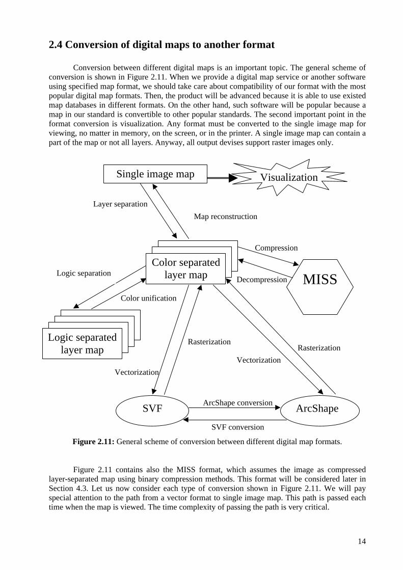
Conversion between different digital maps is an important topic. The general scheme of conversion is shown in Figure 2.11. When we provide a digital map service or another software using specified map format, we should take care about compatibility of our format with the most popular digital map formats. Then, the product will be advanced because it is able to use existed map databases in different formats. On the other hand, such software will be popular because a map in our standard is convertible to other popular standards. The second important point in the format conversion is visualization. Any format must be converted to the single image map for viewing, no matter in memory, on the screen, or in the printer. A single image map can contain a part of the map or not all layers. Anyway, all output devises support raster images only.

Figure 2.11: General scheme of conversion between different digital map formats.

Figure 2.11 contains also the MISS format, which assumes the image as compressed layer-separated map using binary compression methods. This format will be considered later in Section 4.3. Let us now consider each type of conversion shown in Figure 2.11. We will pay special attention to the path from a vector format to single image map. This path is passed each time when the map is viewed. The time complexity of passing the path is very critical.

SVF conversion

ArcShape conversion

Rasterization Rasterization

Vectorization Vectorization

Decompression

Compression

Color unification

Layer separation

Single image map Visualization

Color separated layer map

Logic separated layer map

MISS

Map reconstruction

Logic separation

SVF ArcShape

15

Layer separation: If a single map contains a few colors, the layer separation is very simple. Pixels with different colors are copied to different binary files, and one color is defined as a background color. The number of layers depends on the number of colors in the image. Filtering is applies if specified number of layers is less than number of colors in the image. Map reconstruction: Map reconstruction is a simple process: the image is covered layer by layer. The map reconstruction takes trivial time. Thus, the time of map visualization from any format depends on the speed of conversion from the format to the layer-separated map. Logic separation: There is no perfect way to make logical layer separation because the logic depends on the semantic content of the map. Thus, logical separation can only be done using human resources. From information point of view, color and logic layer separated maps have the same structure. We will consider conversion with a color separated map implying that the same conversion exists for the logically separated map. Color unification: Color unification is very easy, opposite the inverse conversion. Logical layers with the same color are united to one color layer. Compression and decompression: The map is compressed and decompressed layer by layer to and from one MISS file. In addition, MISS format supports compression and decompression of partial of the map. Decompression time depends on the map size. Therefore, visualization of the small part is fast. Raster compression will be considered more detailed in Section 4.3. Vectorization: Vectorization is very difficult task. There are some algorithms based on the shape recognition theory [13] but we will not consider vectorization in this research. Rasterization: Rasterization is one of the topics of this research. Section 3 considers the problem very deeply, gives algorithms and proposes the problem solution. Rasterization task is divided into two subtasks: reading primitives and their attributes form the vector format, and to rasterize the primitives using such algorithms as drawing line, drawing circle and arc, filling areas, etc. The second task is more difficult and can take a lot of time. Therefore, the time of vector map visualization can be long. Thus, vector maps can not be used in low speed and low memory computers even if vector format itself has many good properties. ArcShape conversion

Conversion between vector formats is not difficult, but the formats features should be taken into account. There are three basic features of ArcShape format:

1. ArcShape format does not support the following primitive types: rectangle, circle, arc and Bezier curve. Rectangles and circles are replaced by polygons; arcs and Bezier curves are replaced by polylines.

2. Primitive attributes must be separated from a geometrical primitive and inserted into appropriate database file.

3. Polygons with holes are drawn using background color in SVF format. Thus, the order of vertices must be specified depending on the polygon color. Some polygons are united into one polygon as different parts of the polygon.

16

SVF conversion

The conversion to SVF format includes the following tasks: 1. Convertor has to collect all primitive features from database and legend files and to put

them in one file with the primitive. 2. ArcShape format uses order of vertices for drawing a polygon with a hole. Therefore, the

parts on a polygon must be converted into separated polygons. A polygon color depends on the order of vertices.

3. Sometimes, ArcShape format uses raster graphics inside. For example, a point can represent a topological sign. The topological sign is drawn using a raster image. This image must be vectorized during the conversion to SVF format. Thus, SVF conversion includes elements of vectorization. Therefore, SVF conversion can be quite complicated task.

Very popular idea nowadays is to mix vector and raster approaches in one map [25]. For

example, a raster map can have vector representation of the text. This approach allows having a small time of visualization as a raster map and good scaling of the text as a vector map. Such maps are not considered in this paper but it could be a progressive topic for new research.

17

Chapter 3 From vector to raster

This chapter considers the rasterization process as a basic subject of this paper. Software Convertor [24] was developed according to the ideas and algorithms presented in this chapter. We start by discussion the role of rasterization in a mobile map service application. After that, we consider basic ideas and useful approaches in the rasterization. Next, we describe algorithms of drawing vector primitives in the raster image. Polygon filling algorithm and Hershey vector font output algorithm are developed by Viktor Veis. Finally, we think about the problems that occur during the rasterization of ArcShape maps.

The first part explains the role of rasterization in the DYNAMAP project [8], defines the

tasks to be solved using rasterization and introduces the software tools implemented for the rasterization. The second part defines operations to be done in map rasterization. It proposes a rasterization approach, which uses a format independent vector structure. In addition, the second part gives specification of layer-separated raster map, which will be used later in this thesis. The third part gives algorithms for drawing point, line, polygon, circle, arc, Bezier curve and making text output in the raster image. The fourth part recognizes and solves problems involved in the rasterization of maps from ArcShape format.

18

3.1 Goals of the rasterization

We will consider next the conversion from vector formats to layer separated raster format as needed in the DYNAMAP project. The output of the rasterization is a set of binary images in PBM format. Other map information is stored in the project file. The project file structure was developed by Pavel Kopylov and the rasterization software Convertor by Seppo Nevalainen and Viktor Veis. Seppo concentrated on the SVF format and I took care about the ArcShape format and the drawing routines. The goal of the DYNAMAP project is development of follow areas:

1. Dynamic map handling 2. Conversion between image types 3. Development of efficient zooming operations 4. Building a pilot application

Convertor plays a part in the second and little bit in the third parts of the project. The

project uses MISS format for storing, browsing and transferring maps. There are a lot of map databases in vector formats. The application has to be able to support such databases. Conversion from vector format to MISS format goes via layer-separated map (see Figure 2.11). Convertor performs the rasterization step. The compression is considered in Section 4.2.

Let us first see how the Convertor implements zooming capability. A vector map covers

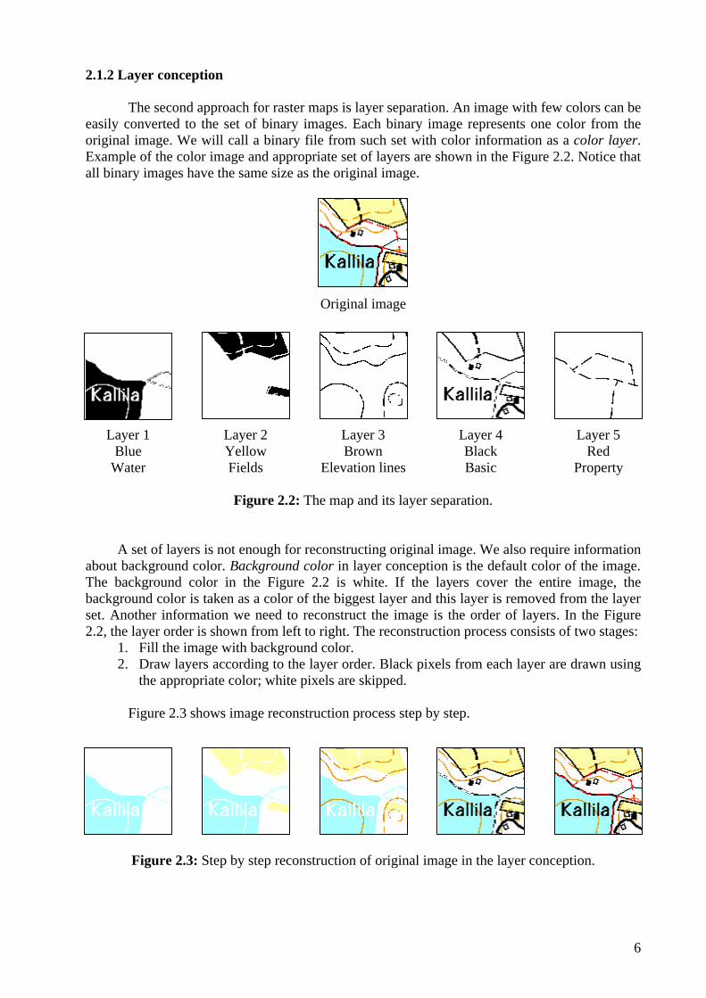
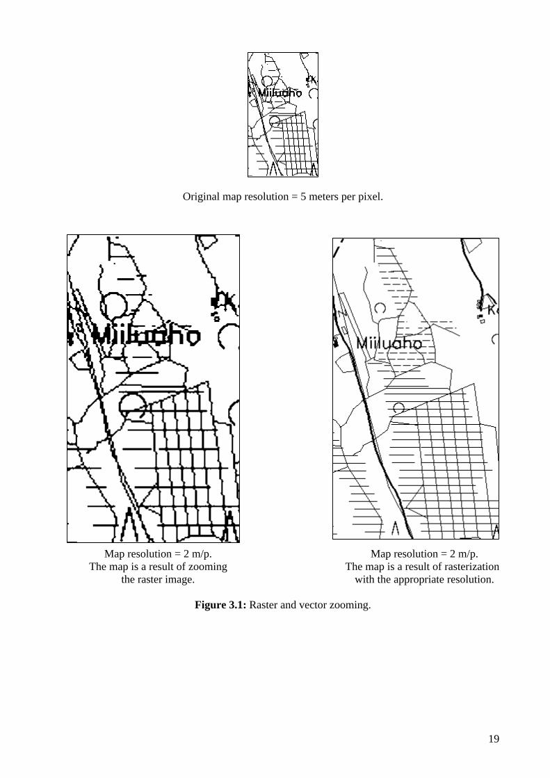
all scales of the region it represented. Raster map represents different scales using several images of different resolution. Map resolution is a parameter of the rasterization. Thus, good quality map scaling or zooming can be done by conversion a vector map with required resolution. Figure 3.1 shows a map with the same resolution (two meters per pixel). Zooming of the left map was done using raster zooming operation from five meters per pixel map. Zooming of the right map was performed by rasterization with appropriate resolution. The quality of right map is much better than the quality of the left map.

19

Original map resolution = 5 meters per pixel.

Map resolution = 2 m/p. Map resolution = 2 m/p. The map is a result of zooming The map is a result of rasterization the raster image. with the appropriate resolution.

Figure 3.1: Raster and vector zooming.

20

3.2 Basic ideas of rasterization

Let us remind features of vector and raster maps and define things to be done in rasterization. Figure 3.2 demonstrates the basic scheme of rasterization. Arrows shows a way of finding a value of the parameter of the raster map. All parameters must be found for correct rasterization.

Vector map

Attributes

Primitives

Color

Text

Type

Style

Etc.

Raster map

Binary images

Geographical info

Size

Layer separation

Colors

Resolution

Background color

ParametersResolution

Layer separation

Figure 3.2: Basic scheme of rasterization. Steps of finding the parameters are explained in the following:

1. Separate primitives for each output layer using the color feature from the attributes. Logic layer separation can be presented by using another feature, for example a type of the primitive (LUOKKA). A type of layer separation is a parameter of rasterization.

2. The resolution is a parameter of the rasterization. 3. Geographical information (coordinates of the two corner points of the bordered box of

the map) is stored in the vector map with the primitives. Coordinates can be stored in different coordinates systems. Then, coordinates should be converted to the required coordinate system. Convertor uses latitude-longitude system to be universal.

4. Geographical information should be converted to some planar coordinate system for founding a size of the binary images. We can calculate size of binary images using formulas (1), (2).

21

−

=resolution

xleftgeoxrightgeoroundwidthbitmap

_____ (1)

−

=resolution

ybottomgeoytopgeoroundheighbitmap

_____ (2)

Here (geo_right_x,geo_top_y) is a coordinate of the top right corner of the bordered box, (geo_left_x,geo_bottom_y) is a coordinate of the bottom left corner of the bordered box, resolution is a parameter of the rasterization.

5. Background color is taken from attributes. 6. All primitives are drawn in the appropriate layer using their attributes.

3.2.1 Format independent vector structure

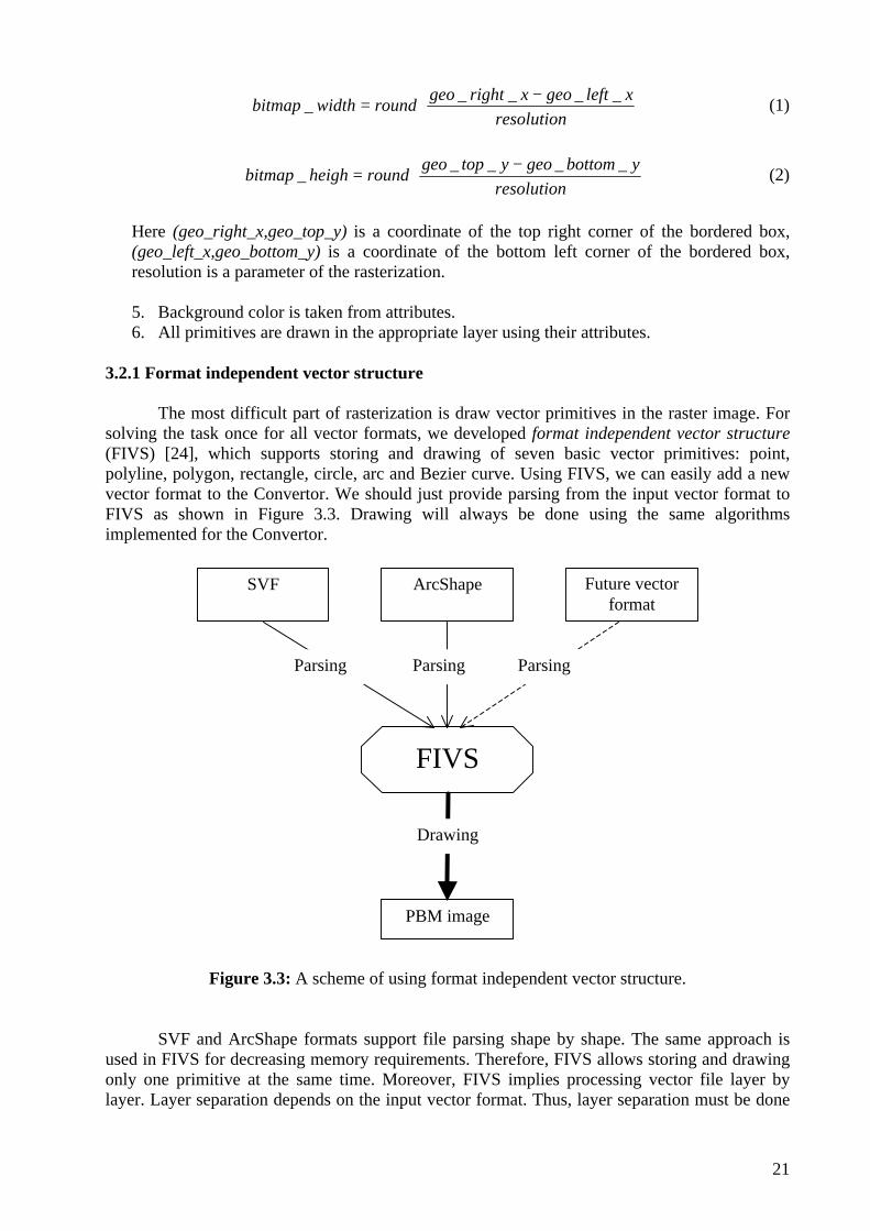
The most difficult part of rasterization is draw vector primitives in the raster image. For solving the task once for all vector formats, we developed format independent vector structure (FIVS) [24], which supports storing and drawing of seven basic vector primitives: point, polyline, polygon, rectangle, circle, arc and Bezier curve. Using FIVS, we can easily add a new vector format to the Convertor. We should just provide parsing from the input vector format to FIVS as shown in Figure 3.3. Drawing will always be done using the same algorithms implemented for the Convertor.

Figure 3.3: A scheme of using format independent vector structure.

SVF and ArcShape formats support file parsing shape by shape. The same approach is used in FIVS for decreasing memory requirements. Therefore, FIVS allows storing and drawing only one primitive at the same time. Moreover, FIVS implies processing vector file layer by layer. Layer separation depends on the input vector format. Thus, layer separation must be done

PBM image

SVF ArcShape Future vector format

FIVS

Parsing Parsing Parsing

Drawing

22

on the parsing stage of the vector map conversion. FIVS structure can be used in the rasterization as follows:

INIT (FIVS) REPEAT

READ_IMAGE_HEADER (FIVS) INIT_PBM_IMAGE (IMAGE) WHILE (NOT READ_SHAPE (FIVS)=0) SHAPE_TO_RASTER (FIVS,IMAGE) SAVE_PBM_IMAGE (IMAGE) FREE_PBM_IMAGE (IMAGE)

UNTIL (NEXT_LAYER (FIVS)!=0) FREE (FIVS)

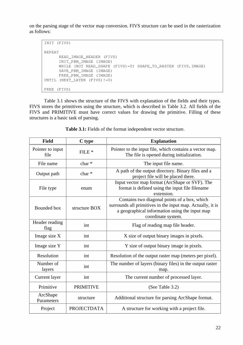
Table 3.1 shows the structure of the FIVS with explanation of the fields and their types.

FIVS stores the primitives using the structure, which is described in Table 3.2. All fields of the FIVS and PRIMITIVE must have correct values for drawing the primitive. Filling of these structures is a basic task of parsing.

Table 3.1: Fields of the format independent vector structure.

Field C type Explanation

Pointer to input file FILE * Pointer to the input file, which contains a vector map.

The file is opened during initialization.

File name char * The input file name.

Output path char * A path of the output directory. Binary files and a project file will be placed there.

File type enum Input vector map format (ArcShape or SVF). The

format is defined using the input file filename extension.

Bounded box structure BOX

Contains two diagonal points of a box, which surrounds all primitives in the input map. Actually, it is

a geographical information using the input map coordinate system.

Header reading flag int Flag of reading map file header.

Image size X int X size of output binary images in pixels.

Image size Y int Y size of output binary image in pixels.

Resolution int Resolution of the output raster map (meters per pixel).

Number of layers int The number of layers (binary files) in the output raster

map.

Current layer int The current number of processed layer.

Primitive PRIMITIVE (See Table 3.2)

ArcShape Parameters structure Additional structure for parsing ArcShape format.

Project PROJECTDATA A structure for working with a project file.

23

Table 3.2: Fields of the PRIMITIVE structure.

Field C type Explanation

Shape enum Type of the primitive: POINT, POLYLINE,

POILYGON, RECTRANGLE, CIRCLE, ARC and BEZIER.

Number of coordinates int The number of basic values, which describe the

primitive

Coordinates int * Array of basic values of the primitive. Polygon parts are separated by flag –1

Color RGB A color of the primitive

Width int A width of the primitive

Properties structure Additional primitive attribute as text, line style, fill style, etc.

3.2.2 Project file

Let us now consider items, which are stored in the project file. Such items are described in Table 3.3. Project file is a text file. Each record starts from a new line and has common structure Parameter=Value. We can see that a project file and a set of binary layer images is a raster map with color layers separation, as we defined in Section 2.2. An example of the project file is considered in Section 5.

Table 3.3: Structure of the project file.

Parameter Value

# Comment

Input= Full name of the input vector map file

Output= Name of the output raster map

Background= Background color as integer R|G|B

LeftBottomX= Latitude of the left bottom point of the map

LeftBottomY= Longitude of the left bottom point of the map

RightTopX= Latitude of the right top point of the map

RightTopY= Longitude of the right top point of the map

Layer i= The name of the layer number i

Color i= R,G,B Red, green and blue components of the color of the layer number i

24

3.3 Graphics library

Drawing stage is the most difficult part of the rasterization process. Let us now think about tools we need to support drawing of all primitives in vector graphics. First of all, we have to have a tool for drawing a point in the image. Let us assume that we already have such tool. We assume that two routines MARK_PIXEL(x,y) and CLEAR_PIXEL(x,y) are existing. Routine MARK_PIXEL (x,y) makes a black pixel with position (x,y). Routine CLEAR_PIXEL (x,y) makes the pixel white. These routines were developed for binary images. All further algorithms are built on these routines. The algorithm can be expanded to grayscale and color image by replacing these primitives to SET_COLOR (X,Y,COLOR).

We should also have algorithms for drawing a line specified by two points for drawing

polylines, rectangles and a polygon border. We require also algorithms for filling areas and filling polygons depending on the order of vertices for drawing all types of polygon primitives. After solid lines and areas, we will consider different line styles and filling styles. Algorithms of drawing circles and arcs are also required. Finally, we must have an algorithm for converting from a Bezier curve to a polyline, which is a standard approach for drawing Bezier curve. Sometimes, we need ability to draw a text and another images. The algorithms should be as fast as possible. The overall rasterization time highly depends on the time complexity of drawing algorithms. Let us create a list of required routines and consider algorithms for them:

1. LINE (x1,y1,x2,y2) — draw a line between two points. 2. FILL_AREA(x,y,color) — fill an area with specified color. Filling begins from point (x,y).

Area is in bordered some way. Another name of the algorithm is flood fill algorithm. 3. FILL_POLYGON(Vertices) — draw a polygon with specified order of vertices (for

example polygons in ArcShape format). 4. CIRCLE (x,y,r) — draw a circle with the center (x,y) and the radius r. 5. ARC (x,y,r,a1,a2) — draw an arc, which starts from the angle a1 and ends the angle a2. 6. TEXT(x,y,text) — output a text in specified position. 7. PLOT_IMAGE(x,y,image) — draw another image on the specified position. 8. POLYLINE BEZIER_TO_POLYLINE (BEZIER) — convert a Bezier curve to a polyline.

3.3.1 Scale problem We will assume that all primitives are scaled to raster map before drawing. Primitives are represented using their basic values in vector map. Basic values are stored in some geographical coordinate system. We want to convert point coordinates and distances to the raster map scale. It is easy to do if we know a bordered box of the vector map and a size of the raster map. Bordered box is a parameter of the vector map. Resolution is a parameter of the rasterization. Conversion can be done according to formulas (3), (4). Formula (4) is inversed about formula (3) because vertical coordinates increase up in geographical coordinate systems and decrease on computer screen.

−

=resolution

xgeogeoxroundbitmapx

min____ (3)

−

=resolution

geoyygeoroundbitmapy

_max___ (4)

25

3.3.2 Line drawing algorithm

Lines, circles and arcs are drawn using Bresenham algorithm [15]. This algorithm is very fast because it uses just integer values and only addition and subtraction operations. The algorithm is shown below.

PROCEDURE LINE(x1,y1,x2,y2) DX <– X2-X1 DY <– Y2-Y1 IX <– ABS(DX) IY <– ABS(DY) INC <– MAX(IX,IY) PLOTX <– X1 PLOTY <– Y1 X=0 Y=0 MARK_PIXEL(PLOTX,PLOTY) FROM I <– 1 TO INC

X <– X+INC Y <– Y+INC PLOT <– FALSE IF (X>=INC)

PLOT <– TRUE X <– X–INC IF (DX>0) PLOTX <– PLOTX+1 ELSE PLOTX <– PLOTX-1

IF (Y>=INC) PLOT <– TRUE Y <– Y–INC IF (DY>0) PLOTY <– PLOTY+1 ELSE PLOTY <– PLOTY-1

IF (PLOT) MARK_PIXEL(PLOTX,PLOTY) 3.3.3 Area filling algorithm

We describe the algorithm for filling a bordered area. We are dealing only with binary images, which have two colors: black=1, white=0. Then, another color (BORDER_COLOR) can be reserved for specifying a border. The algorithm needs a start point for filling. This point and its vertical and horizontal neighbors must be filled if they are inside the image and not on the border. After this, filled neighbors are considered as start points and filling is continued. A pixel is not considered as a start point if the pixel is already filled. It is marked using a special color MARK_FILLED. This process is called a stack phase of filling. After that, border and marked pixels are repainted to FILL_COLOR. We need a box, which includes all filled area for repainting. The box is calculated during the stack stage of filling using two routines:

1. CREATE (BOX,X,Y) — Create a box, which includes just one pixel (X,Y). 2. EXTEND (BOX,X,Y) — Extend the box for including a new pixel (X,Y).

There are two approaches to implement the filling algorithm. First approach is based on

recursion and the second approach is designed using a stack. Convertor program uses stack approach because it is faster. The stack of points is a structure, which supports the following operations:

1. PUT (X,Y) — Put a point into the stack.

26

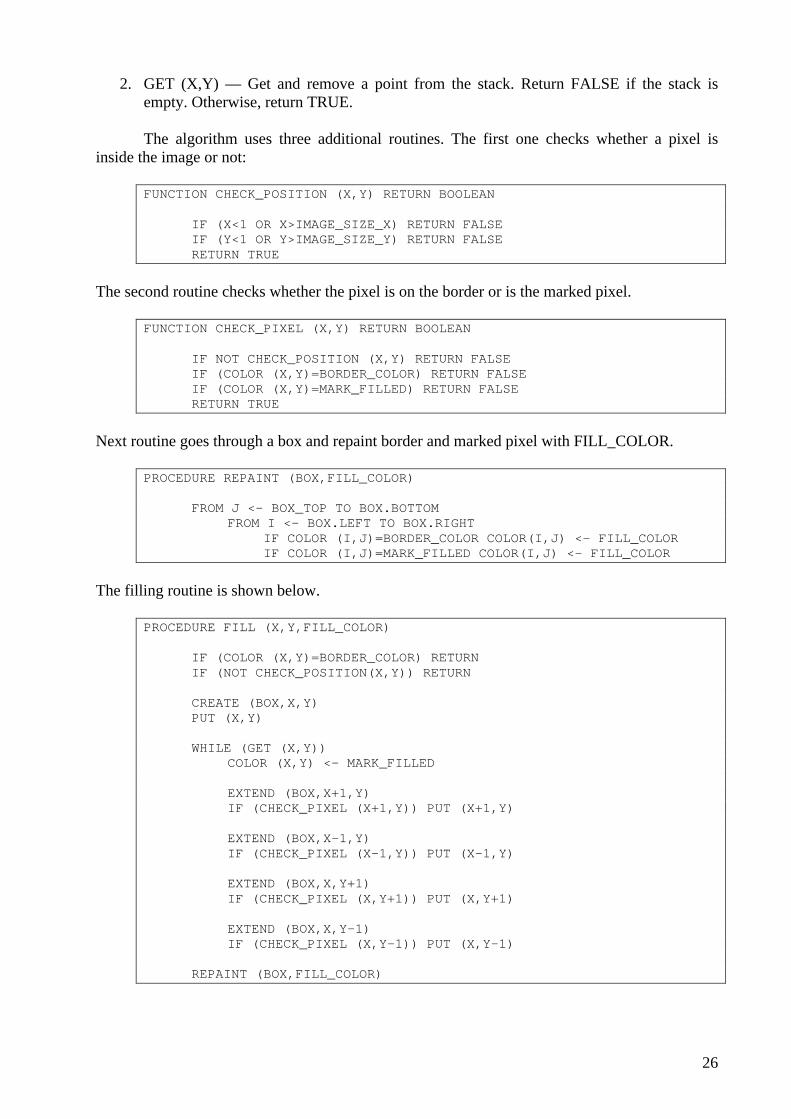
2. GET (X,Y) — Get and remove a point from the stack. Return FALSE if the stack is empty. Otherwise, return TRUE.

The algorithm uses three additional routines. The first one checks whether a pixel is

inside the image or not:

FUNCTION CHECK_POSITION (X,Y) RETURN BOOLEAN

IF (X<1 OR X>IMAGE_SIZE_X) RETURN FALSE IF (Y<1 OR Y>IMAGE_SIZE_Y) RETURN FALSE RETURN TRUE

The second routine checks whether the pixel is on the border or is the marked pixel.

FUNCTION CHECK_PIXEL (X,Y) RETURN BOOLEAN

IF NOT CHECK_POSITION (X,Y) RETURN FALSE IF (COLOR (X,Y)=BORDER_COLOR) RETURN FALSE IF (COLOR (X,Y)=MARK_FILLED) RETURN FALSE RETURN TRUE

Next routine goes through a box and repaint border and marked pixel with FILL_COLOR.

PROCEDURE REPAINT (BOX,FILL_COLOR)

FROM J <– BOX_TOP TO BOX.BOTTOM FROM I <– BOX.LEFT TO BOX.RIGHT

IF COLOR (I,J)=BORDER_COLOR COLOR(I,J) <– FILL_COLOR IF COLOR (I,J)=MARK_FILLED COLOR(I,J) <– FILL_COLOR

The filling routine is shown below.

PROCEDURE FILL (X,Y,FILL_COLOR)

IF (COLOR (X,Y)=BORDER_COLOR) RETURN IF (NOT CHECK_POSITION(X,Y)) RETURN CREATE (BOX,X,Y) PUT (X,Y) WHILE (GET (X,Y))

COLOR (X,Y) <- MARK_FILLED EXTEND (BOX,X+1,Y) IF (CHECK_PIXEL (X+1,Y)) PUT (X+1,Y) EXTEND (BOX,X–1,Y) IF (CHECK_PIXEL (X–1,Y)) PUT (X–1,Y) EXTEND (BOX,X,Y+1) IF (CHECK_PIXEL (X,Y+1)) PUT (X,Y+1) EXTEND (BOX,X,Y–1) IF (CHECK_PIXEL (X,Y–1)) PUT (X,Y–1)

REPAINT (BOX,FILL_COLOR)

27

3.3.4 Polygon filling algorithm

The most difficult drawing routine is a routine of drawing a polygon with filling depending on the order of vertices. Such polygon contains of a set of parts. Each part is a geometrical polygon. A part is filled inside if the order of vertices is clockwise. The part is filled outside if the order of vertices is counterclockwise. Figure 2.4 demonstrates a polygon with two parts. The area filling is not allowed in this case because it is impossible to found the start point for all kinds of polygons.

Let us consider one horizontal line from a polygon border. A polygon border is a closed

curve. This leads that each border pixel has two neighbor pixels. Let us imagine that we are following a polygon border pixel by pixel using the order of vertices. Then, for each horizontal line we will have a border pixel before the line and after the line. They are situated on the neighbor lines (one pixel up or one pixel down). We are interesting in directions of coming to the line and leaving the line. There are eight possible cases of different direction types. They are shown on Figure 3.4. Each case in Figure 3.4 is marked using two codes. The first code specifies a position of the neighbor pixel before the line according to the order of vertices. The second code specifies position of the pixel after the line. For example code LD, RD means that the first neighbor is situated in the left-down direction of the line. The second neighbor pixel is situated on the right-down direction of the line. Notice that a horizontal line can consist just of one pixel.

Case 1 Case 2 Case 3 Case 4 LD, RD RD, LD UT, RU RU, LU

Case 5 Case 6 Case 7 Case 8 LD, RU RU, LD LU, RD RD, LU Figure 3.4: All cases of direction of coming and leaving a horizontal line in the polygon border.

Let us think how the horizontal line of the polygon border changes filling status of pixels before the line and after the line. In first two cases, we are dealing with a local maximum of the border. In case one, filled area is below the horizontal line. In case two, filled area is above. Anyway, the border does not change filling status in the horizontal line in these cases. The same situation is for the local minimum, which we have in the third and fourth cases.

Filled area is situated on the right direction from the border in the fifth case and in the

eighth case. The filling in the horizontal line must be started after the border (look from left to right). Let us mark right pixel of the horizontal line on the border as START_PIXEL. In both cases, the first neighbor pixel is placed lower than the horizontal line. The second neighbor is placed above. Such order of pixels will be a criterion of the start pixel.

In the cases six and seven, we have an opposite situation. Filled area is located on the left

side of the border and we will mark the left pixel of the horizontal line on the border as END_PIXEL. The criterion of the end pixel is the first pixel above and the second pixel below.

28

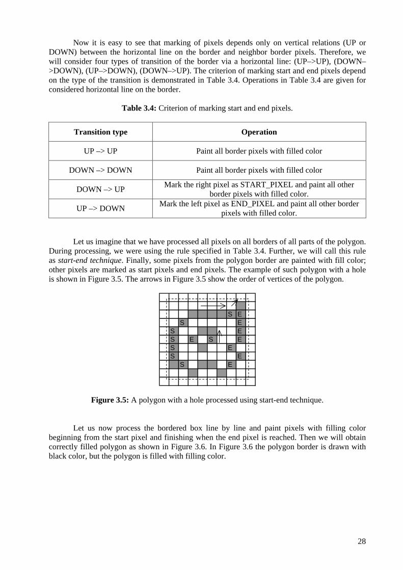
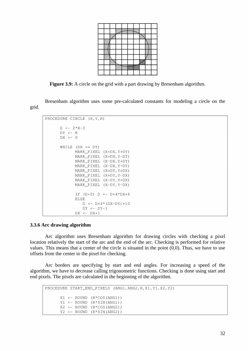
Now it is easy to see that marking of pixels depends only on vertical relations (UP or DOWN) between the horizontal line on the border and neighbor border pixels. Therefore, we will consider four types of transition of the border via a horizontal line: (UP–>UP), (DOWN–>DOWN), (UP–>DOWN), (DOWN–>UP). The criterion of marking start and end pixels depend on the type of the transition is demonstrated in Table 3.4. Operations in Table 3.4 are given for considered horizontal line on the border.

Table 3.4: Criterion of marking start and end pixels.

Transition type Operation

UP –> UP Paint all border pixels with filled color

DOWN –> DOWN Paint all border pixels with filled color

DOWN –> UP Mark the right pixel as START_PIXEL and paint all other border pixels with filled color.

UP –> DOWN Mark the left pixel as END_PIXEL and paint all other border pixels with filled color.

Let us imagine that we have processed all pixels on all borders of all parts of the polygon. During processing, we were using the rule specified in Table 3.4. Further, we will call this rule as start-end technique. Finally, some pixels from the polygon border are painted with fill color; other pixels are marked as start pixels and end pixels. The example of such polygon with a hole is shown in Figure 3.5. The arrows in Figure 3.5 show the order of vertices of the polygon.

S ES E

S ES E S ES ES E

S E

Figure 3.5: A polygon with a hole processed using start-end technique.

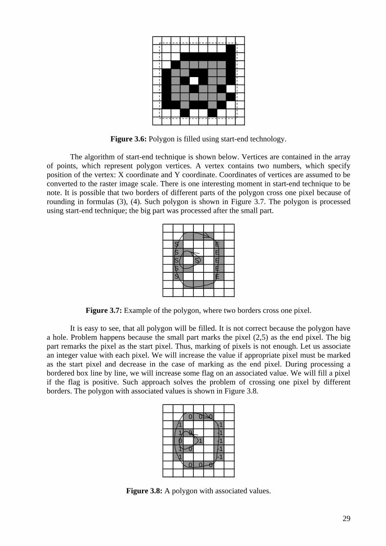
Let us now process the bordered box line by line and paint pixels with filling color beginning from the start pixel and finishing when the end pixel is reached. Then we will obtain correctly filled polygon as shown in Figure 3.6. In Figure 3.6 the polygon border is drawn with black color, but the polygon is filled with filling color.

29

Figure 3.6: Polygon is filled using start-end technology.

The algorithm of start-end technique is shown below. Vertices are contained in the array of points, which represent polygon vertices. A vertex contains two numbers, which specify position of the vertex: X coordinate and Y coordinate. Coordinates of vertices are assumed to be converted to the raster image scale. There is one interesting moment in start-end technique to be note. It is possible that two borders of different parts of the polygon cross one pixel because of rounding in formulas (3), (4). Such polygon is shown in Figure 3.7. The polygon is processed using start-end technique; the big part was processed after the small part.

S ES ES S ES ES E

Figure 3.7: Example of the polygon, where two borders cross one pixel.

It is easy to see, that all polygon will be filled. It is not correct because the polygon have a hole. Problem happens because the small part marks the pixel (2,5) as the end pixel. The big part remarks the pixel as the start pixel. Thus, marking of pixels is not enough. Let us associate an integer value with each pixel. We will increase the value if appropriate pixel must be marked as the start pixel and decrease in the case of marking as the end pixel. During processing a bordered box line by line, we will increase some flag on an associated value. We will fill a pixel if the flag is positive. Such approach solves the problem of crossing one pixel by different borders. The polygon with associated values is shown in Figure 3.8.

0 0 01 -11 0 -10 1 -11 0 -11 -1

0 0 0

Figure 3.8: A polygon with associated values.

30

Let us now think how we can associate values in the binary image. We will use the same approach as we used in the algorithm of filling the area. There are two additional colors were brought into play there. We have enough additional colors (one pixel takes one byte space). Let us specify three constants: MIDDLE — the middle color is equivalent of zero in associated values, MAX_START — the maximum color represented the start pixel, MIN_END — the minimum color represented the end pixel. Experiments conclude that the color range, which is equal five, is more than enough. There are two routines further. They mark start and end pixels using specified constants. The routines are used in the filling algorithm.

PROCEDURE MARK_START (X,Y) IF (COLOR (X,Y)=MAX_START) FAIL IF (COLOR (X,Y)<MIN_END) COLOR(X,Y) <– MIDDLE+1 COLOR (X,Y) <– COLOR (X,Y)+1

PROCEDURE MARK_END (X,Y)

IF (COLOR (X,Y)=MIN_END) FAIL IF (COLOR (X,Y)<MIN_END) COLOR(X,Y) <– MIDDLE–1 COLOR (X,Y) <– COLOR (X,Y)–1

The algorithm fills a polygon with black color. White color is not needed in filling a

polygon depends on the order of vertices. Algorithm makes use of three additional routines. The first routine fills a polygon processing line by line as demonstrated in Figure 3.6. This is a final step of filling a polygon using the order of vertices.

PROCESS_FILL (BOX)

FILL_FLAG=0 FROM J <– BOX_TOP TO BOX.BOTTOM

FROM I <– BOX.LEFT TO BOX.RIGHT

IF (COLOR (I,J)>=MIDDLE_COLOR) FILL_FLAG=FILL_FLAG+COLOR(I,J)-MIDDLE_COLOR MARKPIXEL(I,J)

IF (COLOR (I,J)<MIDLE_COLOR AND COLOR (I,J)>=MIN_END_COLOR)

FILL_FLAG=FILL_FLAG–(MIDDLE_COLOR– COLOR (I,J)) MARKPIXEL(I,J)

IF (FILL_FLAG>0) MARKPIXEL(I,J)

Polygon border is a closed polyline specified by a set of vertices. Thus, we will draw a

border using line algorithm mentioned above. Nevertheless, the function of marking a border pixel will be a new for supporting start-end technique. Such routine is called MARK_PIXEL_SE. Marking of the pixel depends on previous horizontal line. Previous horizontal line specifies using its start X position, end X position and Y coordinate of the line. They are parameters of the routine. Another parameter is a direction of achieving the current horizontal line. The routine extends current line if marked pixel is in the current horizontal line. Otherwise, the routine marks appropriate pixel in the current line according to the rule from Table 3.4.

The line routine, which calls MARK_PEXEL_SE routine for marking a pixel, is called

LINE_SE. It also takes last horizontal line as a parameter because a line between two vertices

31

and a horizontal line are independence. A border is processed pixel by pixel, but not line-by-line in start-end technique.

PROCEDURE MARK_PIXEL_START_END (X,Y,X_MIN,X_MAX,LAST_Y,IN_DIR)

IF (COLOR (X,Y)=0) MARK_PIXEL(X,Y)

IF (Y=LAST_Y) IF (X<X_MIN) X_MIN <– X IF (X>X_MAX) X_MAX <– X RETURN

IF (Y<LAST_Y) OUT_DIR= <– UP ELSE OUT_DIR <– DOWN IF (IN_DIR=DOWN AND OUT_DIR=UP) MARK_START (X_MAX,LAST_Y) IF (IN_DIR=UP AND OUT_DIR=DOWN) MARK_END (X_MIN,LAST_Y) LAST_Y <– Y MIN_X <– MAX_X <– X IF (OUT_DIR=UP) IN_DIR <– DOWN ELSE IN_DIR <– UP

The third routine initializes parameters of a horizontal line. We need this routine for

starting start-end algorithm.

PROCEDURE INIT_HOR_LINE (X,Y,X_MIN,X_MAX,LAST_Y,IN_DIR,PREV_Y)

LAST_Y <– Y MIN_X <– MAX_X <– X IF (PREV_Y<Y) IN_DIR=UP ELSE IN_DIR=DOWN

The final routine, which uses above help routines, is shown below.

PROCEDURE FILL_POLYGON (VERTICES)

CREATE (BOX,VERTICES[0])

FROM N_PART <– 1 TO NUMBER_OF_PARTS–1 INIT_HOR_LINE(VERTICES[0],X_MIN,X_MAX,Y_LAST, VERTICES[NUMBER_OF_VERTICES (N_PART)-1].Y) I <– 0 WHILE (I<NUMBER_OF_VERTICES (N_PART))

LINE_SE (VERTICES[I],VERTICES[I+1], X_MIN,X_MAX,Y_LAST)

EXTEND (BOX,VERTICES[I]) I <– I+1

PROCESS_FILL (BOX)

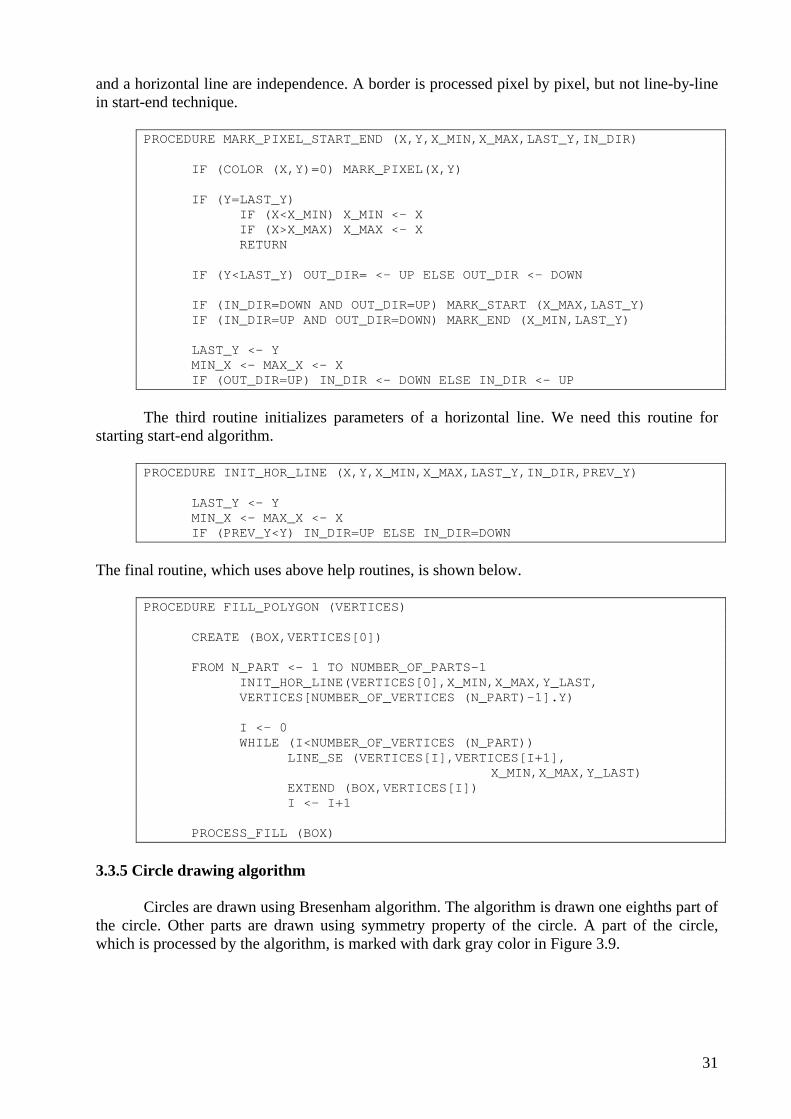
3.3.5 Circle drawing algorithm

Circles are drawn using Bresenham algorithm. The algorithm is drawn one eighths part of the circle. Other parts are drawn using symmetry property of the circle. A part of the circle, which is processed by the algorithm, is marked with dark gray color in Figure 3.9.

32

Figure 3.9: A circle on the grid with a part drawing by Bresenham algorithm.

Bresenham algorithm uses some pre-calculated constants for modeling a circle on the grid.

PROCEDURE CIRCLE (X,Y,R) D <– 2*R-3 DY <– R DX <– 0 WHILE (DX <= DY)

MARK_PIXEL (X+DX,Y+DY) MARK_PIXEL (X+DX,Y–DY) MARK_PIXEL (X–DX,Y+DY) MARK_PIXEL (X–DX,Y–DY) MARK_PIXEL (X+DY,Y+DX) MARK_PIXEL (X+DY,Y–DX) MARK_PIXEL (X–DY,Y+DX) MARK_PIXEL (X–DY,Y–DX) IF (D<0) D <– D+4*DX+6 ELSE

D <– D+4*(DX–DY)+10 DY <– DY–1

DX <– DX+1 3.3.6 Arc drawing algorithm

Arc algorithm uses Bresenham algorithm for drawing circles with checking a pixel

location relatively the start of the arc and the end of the arc. Checking is performed for relative values. This means that a center of the circle is situated in the point (0,0). Thus, we have to use offsets from the center to the pixel for checking.

Arc borders are specifying by start and end angles. For increasing a speed of the

algorithm, we have to decrease calling trigonometric functions. Checking is done using start and end pixels. The pixels are calculated in the beginning of the algorithm.

PROCEDURE START_END_PIXELS (ANG1,ANG2,R,X1,Y1,X2,Y2)

X1 <– ROUND (R*COS(ANG1)) Y1 <– ROUND (R*SIN(ANG1)) X2 <– ROUND (R*COS(ANG2)) Y2 <– ROUND (R*SIN(ANG2))

33

The first checking is very fast and uses dividing a plane by eight parts according to a center of the circle. The dividing is shown in Figure 3.10.

34 2

15

6 87

Figure 3.10: Dividing a plane by eight parts.

Next routine founds a part that a pixel belongs to.

FUNCTION FOUND_PART (X,Y) RETURNS THE NUMBER OF THE PART

IF (X=0 AND Y=0) RETURN 0 IF (X=0 AND Y>0) RETURN 1 IF (X=0 AND Y>0) RETURN 1 IF (X=0 AND Y>0) RETURN 1 IF (X=0 AND Y>0) RETURN 1 IF (X=0 AND Y>0) RETURN 1 IF (X=0 AND Y>0) RETURN 1 IF (X=0 AND Y>0) RETURN 1 IF (X=0 AND Y>0) RETURN 1

If checked pixel and bordered pixels are located in different part of the plane, checking is

performed just comparing the numbers of the parts. Three basic cases, when the part approach is working, are demonstrated in Figure 3.11. The checked pixel is marked by dark gray color in Figure 3.11. Figure 3.11 gives a result of checking for all cases.

3 3 34 2 4 2 4 2

E E E

1 1 15 5 5

6 S 8 6 S 8 6 S 87 7 7

START PART=7 START PART=7 START PART=7 END PART=4 END PART=4 END PART=4 PIXEL PART=8 PIXEL PART=5 PIXEL PART=7 RESULT=YES RESULT=NO RESULT=YES

Figure 3.11: Three basic cases, when the part approach is working.

34

If checked pixel is located in the same part with at least one bordered pixel, we have to use additional measure value m for checking pixels in the same part. The measure is calculated

using the formula ( )yx

yxm =, . Next routine contains a checking algorithm, which includes part

and measuring checking. It must be called for all MARK_PIXEL routines in the routine CIRCLE. Then the arc will be drawn correct.

FUNCTIONCHECK_PIXEL (X,Y,X1,Y1,X2,Y2) RETURN BOOLEAN

P <– FOUND_PART (X,Y) P1 <– FOUND_PART (X1,Y1) P2 <– FOUND_PART (X2,Y2) IF (P=0 OR P1=0 OR P2=0) RETURN FALSE IF (P2<P1)

P2 <– P2+8 IF (P<P1) P <– P+8

IF (P1<P AND P<P2) RETURN TRUE IF (P=P1 AND P IS ODD) RETURN TRUE IF (P=P2 AND P IS ODD) RETURN TRUE M <– X/Y M1 <– X1/Y1 M2 <– X2/Y2 IF (P1>P) IF (P1=P2 AND M1<M2) RETURN TRUE ELSE RETURN FALSE IF (P2<P) IF (P1=P2 AND M1<M2) RETURN TRUE ELSE RETURN FALSE IF (P<P2) IF (M<=M1) RETURN TRUE ELSE RETURN FALSE IF (P1<P) IF (M>=M2) RETURN TRUE ELSE RETURN FALSE IF (M1=M2) IF (M1=M) RETURN TRUE ELSE RETURN FALSE IF (M1>M2) IF (M1>=M AND M>=M2) RETURN TRUE ELSE RETURN FALSE IF (M1<M2) IF (M1>=M OR M>=M2) RETURN TRUE ELSE RETURN FALSE RETURN FALSE

3.3.7 Text output using Hershey vector font

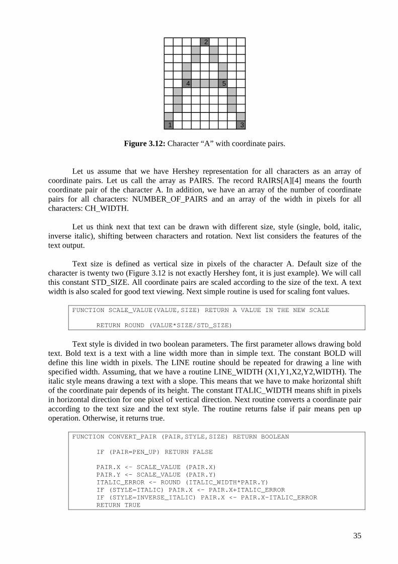
Convertor uses Hershey vector font for drawing a text in rasterization. Full specification of the font can be found in paper [2]. Vector font is useful for scaling, styling and rotation opposite a raster font. Hershey font represents a character as a set of coordinate pairs. The coordinate pair (–1,–1) means pen up operation. Thus, we can use an algorithm of drawing lines for output a text. Figure 3.12 demonstrates the character A with the coordinate pairs marked with dark gray color. The character is represented via six coordinate pairs: (0,0), (5,10), (8,0), (–1, –1), (2,5), (6,5). This information is enough for drawing the character.

35

2

4 5

1 3

Figure 3.12: Character “A” with coordinate pairs.

Let us assume that we have Hershey representation for all characters as an array of coordinate pairs. Let us call the array as PAIRS. The record RAIRS[A][4] means the fourth coordinate pair of the character A. In addition, we have an array of the number of coordinate pairs for all characters: NUMBER_OF_PAIRS and an array of the width in pixels for all characters: CH_WIDTH.

Let us think next that text can be drawn with different size, style (single, bold, italic,

inverse italic), shifting between characters and rotation. Next list considers the features of the text output.

Text size is defined as vertical size in pixels of the character A. Default size of the character is twenty two (Figure 3.12 is not exactly Hershey font, it is just example). We will call this constant STD_SIZE. All coordinate pairs are scaled according to the size of the text. A text width is also scaled for good text viewing. Next simple routine is used for scaling font values.

FUNCTION SCALE_VALUE(VALUE,SIZE) RETURN A VALUE IN THE NEW SCALE

RETURN ROUND (VALUE*SIZE/STD_SIZE)

Text style is divided in two boolean parameters. The first parameter allows drawing bold text. Bold text is a text with a line width more than in simple text. The constant BOLD will define this line width in pixels. The LINE routine should be repeated for drawing a line with specified width. Assuming, that we have a routine LINE_WIDTH (X1,Y1,X2,Y2,WIDTH). The italic style means drawing a text with a slope. This means that we have to make horizontal shift of the coordinate pair depends of its height. The constant ITALIC_WIDTH means shift in pixels in horizontal direction for one pixel of vertical direction. Next routine converts a coordinate pair according to the text size and the text style. The routine returns false if pair means pen up operation. Otherwise, it returns true.

FUNCTION CONVERT_PAIR (PAIR,STYLE,SIZE) RETURN BOOLEAN

IF (PAIR=PEN_UP) RETURN FALSE PAIR.X <– SCALE_VALUE (PAIR.X) PAIR.Y <– SCALE_VALUE (PAIR.Y) ITALIC_ERROR <– ROUND (ITALIC_WIDTH*PAIR.Y) IF (STYLE=ITALIC) PAIR.X <– PAIR.X+ITALIC_ERROR IF (STYLE=INVERSE_ITALIC) PAIR.X <– PAIR.X–ITALIC_ERROR RETURN TRUE

36

A text shift is shifting in pixels between two characters. Let us call this parameter as SHIFT. We will use it further in the algorithm of drawing a text.

Text rotation means rotation of the text around the point of text output. The rotation is

done directly before drawing a line between two coordinate pairs. Net routine makes rotation of a point around another point with some angle in radians using standard a matrix of rotation.

PROCEDURE ROTATE (X,Y,X_CENTER,Y_CENTER,ANGLE) IF (ANGLE=0) RETURN DX <– X–X_CENTER DY <– Y–Y_CENTER C <– COS (ANGLE) S <– SIN (ANGLE) DX_NEW <– DX*C–DY*S DY_NEW <– DX*S+DY*C X=X_CENTER+DX_NEW Y=Y_CENTER+DY_NEW

Now we are ready to write an algorithm for drawing a character with specified size, style

and rotation. The routine processes a character using coordinate pairs, convert them and control pen up operation. The character is drawn using LINE_WIDTH routine. The routine will return a character width in pixels.

FUNCTION DRAW_CHARACTER(CH,X,Y,X_CENTER, Y_CENTER,SIZE,STYLE,ANGLE) RETURN WIDTH

IF (STYLE=BOLD) WIDTH <– BOLD ELSE WIDTH <– 1 WIDTH <– SCALE_VALUE (WIDTH) PEN_UP_FLAG <– TRUE X1 <– Y1 <– X2 <–Y2 <– 0 FOR I <–1 TO NUMBER_OF_PAIRS[CH]

IF (PAIR[CH][I]=PEN_UP) PEN_UP_FLAG <– TRUE CONTINUE

IF (PEN_UP_FLAG)

X1 <– PAIR[CH][I].X Y1 <– PAIR[CH][I].Y CONVERT_PAIR (X1,Y1,STYLE,SIZE) ROTATE (X1,Y1,X_CENTER,Y_CENTER,ANGLE) PEN_UP_FLAG <– FALSE CONTINUE

X2 <– PAIR[CH][I].X Y2 <– PAIR[CH][I].Y CONVERT_PAIR (X2,Y2,STYLE,SIZE) ROTATE (X2,Y2,X_CENTER,Y_CENTER,ANGLE) LINE_WIDTH (X1,Y1,X2,Y2,WIDTH) X1 <– X2 Y1 <– Y2

RETURN SCALE_VALUE (CH_WIDTH)

37

Now it is easy to create routine for drawing a text. It will draw character by character and take care about shifting between characters.

PROCEDURE TEXT (X,Y,TEXT,SIZE,STYLE,ANGLE,SHIFT)

X_CH <– X FROM I=1 TO LENGTH (TEXT)

X_CH <– X_CH+DRAW_CHARACTER (TEXT[I],X_CH,Y,X,Y,SIZE, STYLE,ANGLE)

X_CH <– X_CH+SHIFT 3.3.8 Another image drawing algorithm

The algorithm for drawing an image in another image is very simple. It just copies pixels. There are two modes of coping: ORIGIN and CRYSTAL. Origin mode copies all pixels without any changes. Crystal mode copies just black pixels and allows putting a raster graphics on binary layers. Crystal mode is often to use in rasterization.

PROCEDURE PLOT_IMAGE (X,Y,IMAGE,MODE)

U <– V <– 1 FROM J <– 1 TO IMAGE_SIZE_Y (IMAGE)

FROM I <– 1 TO IMAGE_SIZE_X (IMAGE) IF (MODE=ORIGINAL OR COLOR(I,J)>0)

COLOR (U,V) <– COLOR (IMAGE,I,J) U <– U+1

V <– V+1 3.3.9 Bezier curve algorithm

Bezier algorithm comes to conversion from a Bezier curve to the polyline. The number of vertices of the polyline is a parameter of conversion. Increasing number of vertices makes the polyline more looks like the original Bezier curve. Experiments result that twenty vertices are usually enough. The algorithm is given without mathematical explanation. Full considering of Bezier curve is given here [15]. Parameter BEZIER consists of four points. Their meaning describes in Section 2.3. Bezier conversion is recommended to do before scaling to raster coordinates. This allows increasing conversion fidelity.

FUNCTION BEZIER_TO_POLYLINE (BEZIER, NUMBER_OF_VERTICES) RETURN VERTICES

DT <– 1/(NUMBER_OF_VERTICES–1) FROM K<– 0 TO NUMBER_OF_VERTICES–1

T <– K*DT AT1 <– 1–T AT2 <– AT1*AT1 BT2 <– T*T F0 <– AT1*AT2 F1 <– 3*T*AT2 F2 <– 3*BT2*AT1 F3 <– T*BT2 X <– F0*BEZIER[0].X+F1*BEZIER[1].X+F2*BEZIER[2].X+

+F3*BEZIER[3].X Y <– F0*BEZIER[0].Y+F1*BEZIER[1].Y+F2*BEZIER[2].Y+

38

+F3*BEZIER[3].Y VERTICES[K].X <– ROUND (X) VERTICES[K].Y <– ROUND (Y)

3.3.10 Conclusion

Now we know conversion map parameters and drawing algorithm. This is enough technique for creating a convertor from vector maps to raster maps. The next part considers extracting primitive attributes from ArcShape format.

39

3.4 ArcShape design

This part considers a design of rasterization of the map in ArcShape format provided by NLS. There are two problems in the rasterization ArcShape maps: separation of ArcShape files into layers, and extraction of attributes of the primitives. These two map features depend on the specific realization of the ArcShape format. 3.4.1 File design

ArcShape map consists of a set of files, divided according to the primitive type, the map object type and the location of the primitives in the map. These file features are recognized from the name of the file. Primitives with different locations must be united into one layer. Therefore, different files can be united into one layer depending on the layer separation of rasterization. Moreover, one file can be included into two or more layers. For example, area polygon file contains fields and lakes, which should be rasterized into different layers in the case of color separation (fields are yellow, lakes are blue).

Let us separate ArcShape files into classes depending on the primitive and geographical

types. Primitive type is specified using the first character of the file name. Geographical type is set via the last character. We will designate a class by these two characters, those we will call a class code. For example, the code mp means a class of polygon primitives from areas objects. Each class consists of four files, which represents different location of the map. We will then combine classes into layers.

As we mentioned above, one class can be included into two or more layers. Thus, we

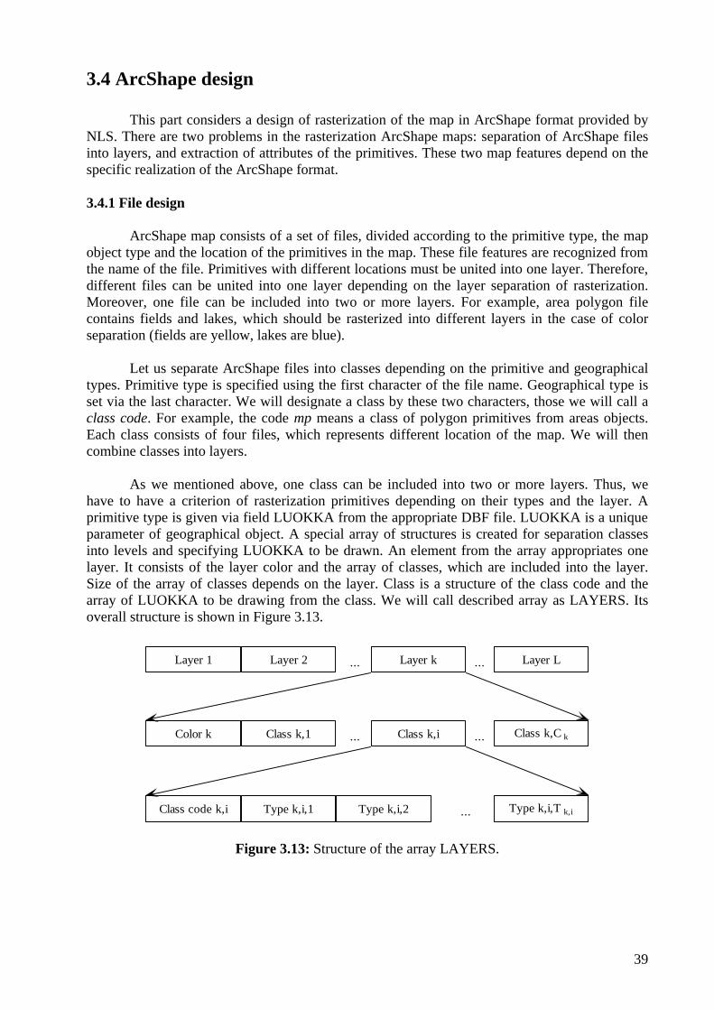
have to have a criterion of rasterization primitives depending on their types and the layer. A primitive type is given via field LUOKKA from the appropriate DBF file. LUOKKA is a unique parameter of geographical object. A special array of structures is created for separation classes into levels and specifying LUOKKA to be drawn. An element from the array appropriates one layer. It consists of the layer color and the array of classes, which are included into the layer. Size of the array of classes depends on the layer. Class is a structure of the class code and the array of LUOKKA to be drawing from the class. We will call described array as LAYERS. Its overall structure is shown in Figure 3.13.

Figure 3.13: Structure of the array LAYERS.

Layer 1 ...Layer 2 Layer k Layer L...

Color k ...Class k,1 Class k,i Class k,C k...

Class code k,i Type k,i,1 Type k,i,2 Type k,i,T k,i...

40

Figure 3.13 uses the following designations: • L — the number of raster layers, • kC — the number of classes in layer k , • kT — the number of types in class i from layer k .

The array LAYERS is created depending on the layer separation, which is a parameter of

the rasterization. Next routine takes the array LAYERS as a parameter and checks a primitive type according to the layer and the class.

FUNCTION CHECK_TYPE(TYPE,LAYERS,LAYER,CLASS) RETURN BOOLEAN

FROM J<– 0 TO NUMBER_OF_TYPES[LAYER][CLASS] IF (TYPE=LAYERS[LAYER].CLASSES[CLASS].TYPES[J])

RETURN TRUE

RETURN FALSE

Next routine processes a vector map layer-by-layer according to specified array LAYERS. This is an abstract level routine. It assumes that we know how to read and rasterize primitives in the binary image.

PROCEDURE RASTER_ARC_SHAPE (LAYERS)

FROM K <– 0 TO NUMBER_OF_LAYERS OPEN_PBM_IMAGE (IMAGE) SET_COLOR (PROJECT,LAYERS[K].COLOR) FROM I <– 0 TO NUMBER_OF_CLASSES[K]

OPEN_FILE (FILE,LAYERS[K][I].CODE) WHILE (NOT ALL_CLASS_FILES_ARE_PROCESSED)

READ_PRIMITIVE (PRIMITIVE,FILE) WHILE (NOT ALL_PRIMITIVE_ARE_PROCESSED)

IF (CHECK_TYPE (PRIMITIVE.LUOKKA, LAYERS,K,I)) DRAW (PRIMITIVE,IMAGE)

READ_NEXT_PRIMITIVE (PRIMITIVE,FILE) OPEN_NEXT_FILE (FILE, LAYERS[K][I].CODE)

3.4.2 Line styles and fill attributes

Now we have a tool for separation of ArcShape files into layers. Let us think about extracting primitive attributes from ArcShape map. Attributes are stored in two files: database files (DBF) and legend files (AVL). Each primitive from the map has appropriate record in the database file.

Other attributes (line style, fill style, etc.) are stored in the legend file. A key for getting these attributes is a primitive type LUOKKA. Unfortunately, a format of the legend files is not specified by ESRI. Thus, we have to provide our own system of getting required attributes from LUOKKA. This is the second task of ArcShape design. There are three different types of attributes: for points, for polylines and for polygons. Text can be drawn using algorithm from Section 3.3 and attributes from the database file.

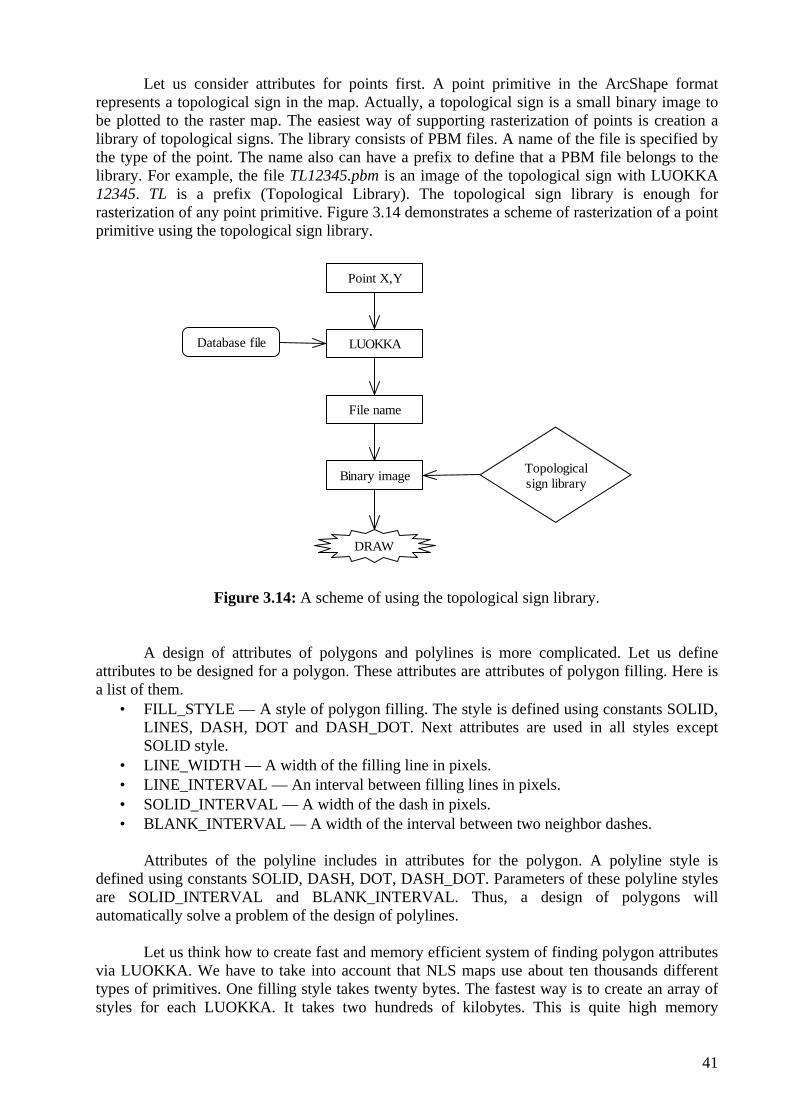
41

Let us consider attributes for points first. A point primitive in the ArcShape format represents a topological sign in the map. Actually, a topological sign is a small binary image to be plotted to the raster map. The easiest way of supporting rasterization of points is creation a library of topological signs. The library consists of PBM files. A name of the file is specified by the type of the point. The name also can have a prefix to define that a PBM file belongs to the library. For example, the file TL12345.pbm is an image of the topological sign with LUOKKA 12345. TL is a prefix (Topological Library). The topological sign library is enough for rasterization of any point primitive. Figure 3.14 demonstrates a scheme of rasterization of a point primitive using the topological sign library.

Figure 3.14: A scheme of using the topological sign library.

A design of attributes of polygons and polylines is more complicated. Let us define attributes to be designed for a polygon. These attributes are attributes of polygon filling. Here is a list of them.

• FILL_STYLE — A style of polygon filling. The style is defined using constants SOLID, LINES, DASH, DOT and DASH_DOT. Next attributes are used in all styles except SOLID style.

• LINE_WIDTH — A width of the filling line in pixels. • LINE_INTERVAL — An interval between filling lines in pixels. • SOLID_INTERVAL — A width of the dash in pixels. • BLANK_INTERVAL — A width of the interval between two neighbor dashes.

Attributes of the polyline includes in attributes for the polygon. A polyline style is

defined using constants SOLID, DASH, DOT, DASH_DOT. Parameters of these polyline styles are SOLID_INTERVAL and BLANK_INTERVAL. Thus, a design of polygons will automatically solve a problem of the design of polylines.

Let us think how to create fast and memory efficient system of finding polygon attributes via LUOKKA. We have to take into account that NLS maps use about ten thousands different types of primitives. One filling style takes twenty bytes. The fastest way is to create an array of styles for each LUOKKA. It takes two hundreds of kilobytes. This is quite high memory

Point X,Y

File name

LUOKKA

Binary image

Database file

Topologicalsign library

DRAW

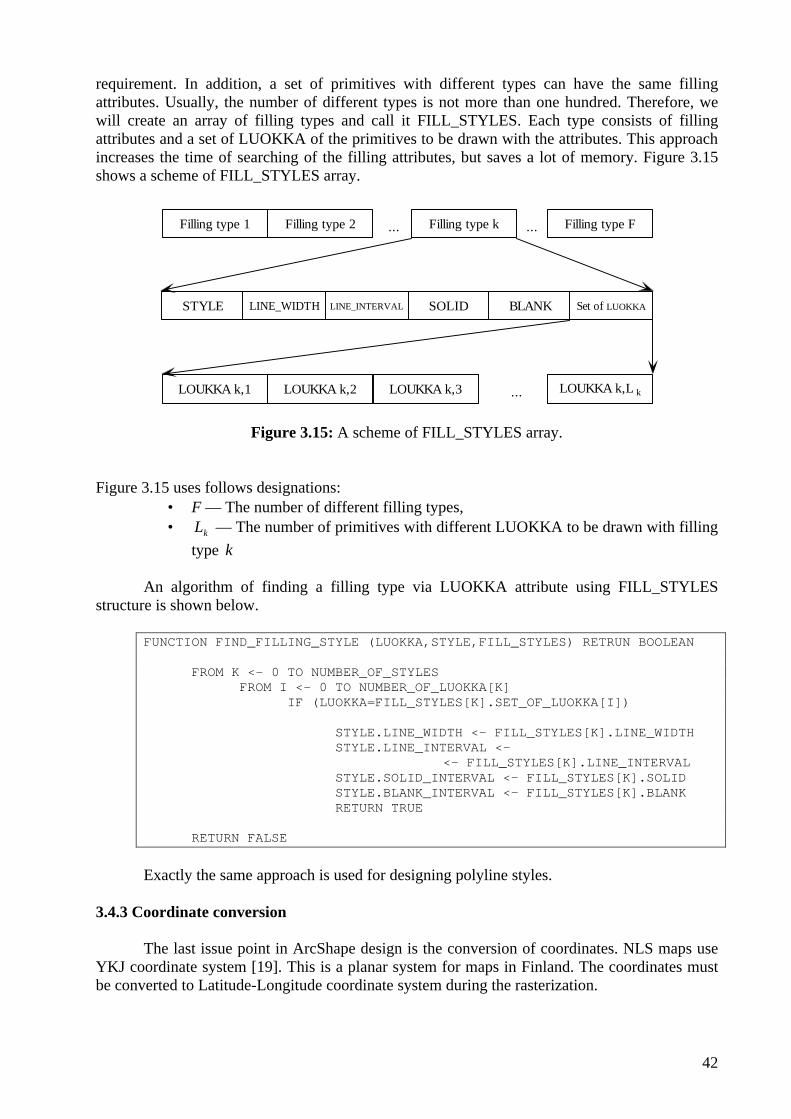
42

requirement. In addition, a set of primitives with different types can have the same filling attributes. Usually, the number of different types is not more than one hundred. Therefore, we will create an array of filling types and call it FILL_STYLES. Each type consists of filling attributes and a set of LUOKKA of the primitives to be drawn with the attributes. This approach increases the time of searching of the filling attributes, but saves a lot of memory. Figure 3.15 shows a scheme of FILL_STYLES array.

Figure 3.15: A scheme of FILL_STYLES array. Figure 3.15 uses follows designations:

• F — The number of different filling types, • kL — The number of primitives with different LUOKKA to be drawn with filling

type k

An algorithm of finding a filling type via LUOKKA attribute using FILL_STYLES structure is shown below.

FUNCTION FIND_FILLING_STYLE (LUOKKA,STYLE,FILL_STYLES) RETRUN BOOLEAN

FROM K <– 0 TO NUMBER_OF_STYLES FROM I <– 0 TO NUMBER_OF_LUOKKA[K]

IF (LUOKKA=FILL_STYLES[K].SET_OF_LUOKKA[I]) STYLE.LINE_WIDTH <– FILL_STYLES[K].LINE_WIDTH STYLE.LINE_INTERVAL <–

<– FILL_STYLES[K].LINE_INTERVAL STYLE.SOLID_INTERVAL <– FILL_STYLES[K].SOLID STYLE.BLANK_INTERVAL <– FILL_STYLES[K].BLANK RETURN TRUE

RETURN FALSE

Exactly the same approach is used for designing polyline styles.

3.4.3 Coordinate conversion

The last issue point in ArcShape design is the conversion of coordinates. NLS maps use YKJ coordinate system [19]. This is a planar system for maps in Finland. The coordinates must be converted to Latitude-Longitude coordinate system during the rasterization.

Filling type 1 ...Filling type 2 Filling type k Filling type F...

STYLE LINE_WIDTH SOLID BLANK

LOUKKA k,1 LOUKKA k,2 LOUKKA k,3 LOUKKA k,L k...

LINE_INTERVAL Set of LUOKKA

43

Now we know enough to create software for rasterization different formats of vector maps. Next chapter will deal with the second stage of the conversion from vector graphics to MISS format.

44

Chapter 4 Map compression

This chapter gives an introduction to image compression, shows basic characteristics of compression and image analysis. Then, we will consider alternative ways of compression vector maps and give some simplification algorithms. Finally, we will consider the compression of raster maps and the concept of putting one map into single file only. We will define the MISS format in detail, describe the structure and discuss the features of the format.

45

4.1 Compression methods

Compression of digital maps is very important subject because huge map databases are stored in servers and map traffic via network communications can be quite high. Therefore, minimizing of the map size allows saving a lot of resources

This part considers overall theory of compression. We will discuss about compression

approaches, classification and parameters of quality of compression methods. Next two parts are devoted to raster map compression and to vector map compression. The biggest resource in raster map is the image of the map. Other information takes typically less than one percent of the entire map size. Thus, the raster map compression means a compression of digital images, which the map includes. Vector map compression deals with geometrical primitives and their attributes. For example, primitives and attributes in a map of ArcShape format usually takes the same space. . There are a lot of methods of compression: Huffman coding [11], arithmetic coding [22], RLE [9], JBIG [12], JPEG [20], etc. We will shortly consider LZW [27] [26], arithmetic coder and JBIG. LZW method [26] is a basis of GIF [16] format. Arithmetic coder and JBIG are used in MISS format [7].

Figure 4.1: A binary image with one black pixel.

Let us consider a binary image shown in Figure 4.1. The image size is 8x8. The image has just one black pixel in the left-top corner. The image takes 6488 =⋅ bits if it is stored pixel-by-pixel as in the binary file. This way of storing the image is redundant. The image can be considered as a set of black pixels. Thus, a position of any pixel is specified by number that is between 1..64. Therefore, we need ( ) 664log2 = bits for each black pixel from the image. The image in Figure 4.1 can be stored in six bits. Consequently, we decreased the image size more than ten times using reorganization of information. In general, compression is transformation of information for decreasing a size for it’s storing. A way of transformation is called a model. The model defines appropriate compression method. Let us consider characteristics of compression:

1. Time of compression 2. Time of decompression 3. Compression efficiently

46

4. Compression error 5. Compression reliability.

The time of compression is not very important in map compression but the time of

decompression is very critical because a speed of visualization directly depends on this parameter. All four characteristics depend on the compressed image. A method of compression is developed and is recommended for specified class of images. Everybody would like to be sure that the method work good for all images from specified class. This is impossible to check directly. Compression reliability is checking during a time of exploiting the method.

An efficiently of compression is merged by compression ratio. It is the ratio of the size of original information to the size of compressed information. Compression is better if the ratio is higher. Compression ratio is calculated using Formula 5.

filecompressedofsize

fileoriginalofsizerationcompressio = (5)

A measure of the compression efficiently of raster images is the bit rate, which gives the

average number of bits per stored pixel of the image:

heightwhidth

filecompressedofsizeratebit

⋅= (bits per pixel). (6)

The compression efficiently increases when the bit rate is decreased. The compression

ratio in our example equals 7.10664 ≈ , and the bit rate equals to 09375.0646 = bits per pixel.

There are two basic types of compression: lossy compression and lossless compression. Lossless compression allows restoring information exactly the same, as it was before compression. Lossy compression loses some part of information, but allows higher compression ratio. There are three basic methods for measuring the compression error [9]: mean absolute error (MAE), mean square error (MSE) and peak-to-peak signal to noise ratio (PSNR):

∑=

−=N

iii xy

NMAE

1

1 (7)

( )∑=

−=N

iii xy

NMSE

1

21 (8)

[ ]MSEPSNR 2

10 255log10 ⋅= , (9) where

• N is the number of pixels in the image, • ix is the value of the pixel from the original image, • iy is the value of the pixel from the restored image.

Measuring of a compression error in vector images is more complicated task. One

method is to rasterize the original and reconstructed images and to compare them using the raster

47

approach. However, the result depends on the resolution. There is no optimal or average resolution. The resolution depends on final user requests. 4.1.1 Modeling

The efficient of the compression method depends on the image. Let show this on the example.

Figure 4.2: A binary image with a set of black pixels.

There are thirty seven black pixels in the image. If we will compress the image using our first model, the compressed size will be 222637 =⋅ bits. The size is increased after compression. Let us try another model: the image is stored as a set of positions of color changing. Assuming, the first pixel have white color. Then, compressed representation of the last image is two values: (0 37). The code takes 12 bits.

The example shows that the efficiency of a compression method depends on the

compressed image. Usually, models have parameters, which are optimized for the image. Any compression method works perfect only for some class of images, for which the method was developed. Process of creation a model calls modeling [9], [17].

Let us come back to our example and code the first model as zero and the second model

as one. Now we will code an image using both models. A model with better result is chosen for storing the image. The first bit is reserved for storing the code of used model. The code of the first image is (0 0). The size of the code equals 1+6=7 bits. The code of the second image is (1 0 37) and a size of the code equals to 13 bits.

Consequently, we built a new model, which is based on two existing models. The process

of developing compression methods is the same. It is based on collecting, combining and improving existing methods. All methods are classified depending on the way of storing the model information:

1. Static methods use standard model for all compressed images. 2. Semi-adaptive methods stores model information with a code. It is two-pass methods. In

the thirst phase, the input data is analyzed and the model is created. The second phase is the actual compression, which uses the model.

3. Adaptive methods create a model during the compression. The model is not stored in the code. It is reconstructed during the decompression.

48

An important conception of compression is the entropy. Entropy is a measure of

information. Let us consider a raster image of N pixels each with k different colors. Equation ( )xn means the number of pixels with the color x. Then the formula ( ) ( ) Nxnxp = gives the

probability of the color x. Equation (10) shows the self-entropy of the color x. ( ) ( )xpxH 2log−= (10) The overall entropy of the image

( ) ( ) ( ) ( )∑∑==

⋅−=⋅=k

x

k

x

xpxpxHxpH1

21

log (11)

is the minimum size of the compressed image in bits. If some method achieved the size of the entropy, it is the optimal method for the image. 4.1.1 Arithmetic coding

Arithmetic coding [22] is known to be optimal coding method in respect to the model. Moreover, it is extremely suitable for dynamic modeling, since there is no actual code table like in Huffman coding to be updated. Let us next consider the fundamental properties of binary arithmetic: n bits represent any natural value from zero to 12 −n . Let consider the interval [0,1], which is divided by n subintervals with the same length nA −= 2 . Any interval can be coded by n bits as shown in Figure 4.3.

1

0

111

110

101

100

011

010

001

000

1

0

11

10

01

000.125

0.25

0.375

0.5

0.625

0.75

0.875

Figure 4.3: Interval [0,1] is divided into 8 parts, thus each having the length of 2-3=0.125. Each interval can now be coded by using − =log .2 0 125 3 bits [9].

The basic idea of arithmetic coding is to represent the entire input file as a small interval in the range [0,1]. The actual coding is the binary code representation of the interval; taking − log2 A bits, in respect to the length of the interval (A). In the other words, arithmetic coding represents the input file with a single codeword.

Let us consider an input file with the length N: Nxxx ....,, 21 , which consists of k different symbols with appropriate probabilities ( ) ( ) ( )kppp ....,2,1 . The interval [ ]1,00 =A is divided by k

49

parts according to the probability model. The interval 1A with the length ( )1xp is chosen according to the first symbol of the input file and is divided using the same probability model. The process is repeated for each symbol to be coded resulting to a smaller and smaller interval. The final interval describes the source uniquely. The length of this interval is the cumulative multiplication of the probabilities of the coded symbols:

( ) ( ) ( ) ( )∏=

=⋅⋅⋅==N

iiNnfinal xpxpxpxpAA

121 ... (13)

Due to the previous discussions this interval can be coded by

( ) ( ) ( )∑∏==

−=−=N

ii

N

ii xpxpAC

12

12 loglog (14)

number of bits (assuming A is a power of ½). If the same model is applied for each symbol to be coded, the code length can be described in respect to the source alphabet:

( ) ( ) ( )∑=

⋅−=k

jjj xpxpAC

12log . (15)

The important observation is that the ( )C A equals to the entropy! 4.1.2 JBIG

JBIG (Joint Bilevel Image Experts Group) [12] is the newest binary image compression standard by CCITT and ISO. It is based on context-based compression where the image is compressed pixel by pixel. The pixels are then coded by arithmetic coding according to their probabilities. The arithmetic coding component in JBIG is the QM-coder (arithmetic coder for binary input with optimization of multiplication operations and own modeling procedures).

7-pixel template 10-pixel template Two-line version ofthe 10-pixel template

Pixel to be coded

Pixel within template

?? ?

?

Figure 4.4: JBIG sequential model templates [9].

Let us consider a pixel from the image and the pixel neighborhood, which we will call a context template, see Figure 4.4. The context of the pixel depends on the colors of the pixels in the context template. Therefore, there are m2 different contexts in binary images, where m is the number of pixels in the template. Let us consider a binary image to be compressed, which includes N pixels. Then the equation ( ) ( ) NCnCp jj = is a probability of the context jC , where

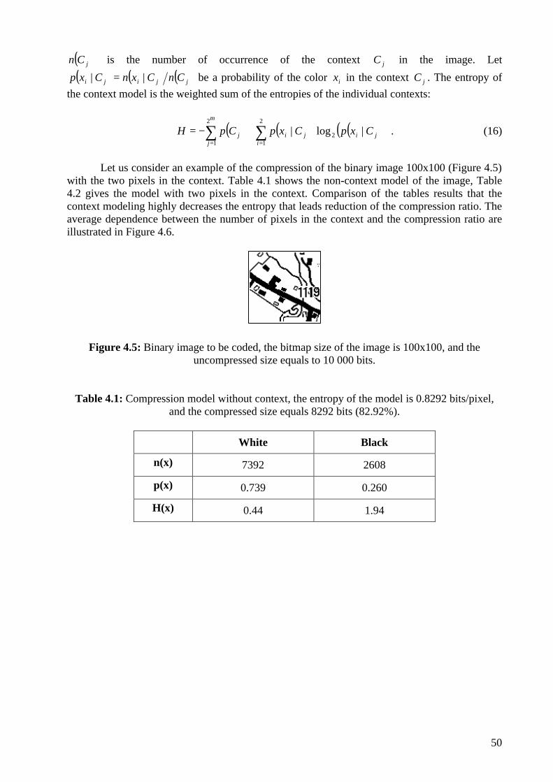
50

( )jCn is the number of occurrence of the context jC in the image. Let

( ) ( ) ( )jjiji CnCxnCxp || = be a probability of the color ix in the context jC . The entropy of the context model is the weighted sum of the entropies of the individual contexts:

( ) ( ) ( )( )∑ ∑= =

⋅⋅−=

m

j ijijij CxpCxpCpH

2

1

2

12 |log| . (16)

Let us consider an example of the compression of the binary image 100x100 (Figure 4.5)

with the two pixels in the context. Table 4.1 shows the non-context model of the image, Table 4.2 gives the model with two pixels in the context. Comparison of the tables results that the context modeling highly decreases the entropy that leads reduction of the compression ratio. The average dependence between the number of pixels in the context and the compression ratio are illustrated in Figure 4.6.

Figure 4.5: Binary image to be coded, the bitmap size of the image is 100x100, and the uncompressed size equals to 10 000 bits.

Table 4.1: Compression model without context, the entropy of the model is 0.8292 bits/pixel, and the compressed size equals 8292 bits (82.92%).

White Black

n(x) 7392 2608

p(x) 0.739 0.260

H(x) 0.44 1.94

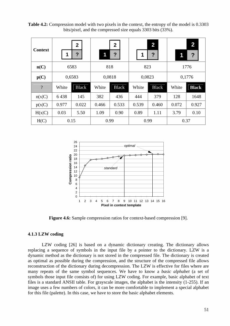
51

Table 4.2: Compression model with two pixels in the context, the entropy of the model is 0.3303 bits/pixel, and the compressed size equals 3303 bits (33%).

Context 2

1 ?

2

1 ?

2

1 ?

2

1 ?

n(C) 6583 818 823 1776

p(C) 0,6583 0,0818 0,0823 0,1776

? White Black White Black White Black White Black

n(x|C) 6 438 145 382 436 444 379 128 1648

p(x|C) 0.977 0.022 0.466 0.533 0.539 0.460 0.072 0.927

H(x|C) 0.03 5.50 1.09 0.90 0.89 1.11 3.79 0.10

H(C) 0.15 0.99 0.99 0.37

02468

101214161820222426

1 2 3 4 5 6 7 8 9 10 11 12 13 14 15 16Pixel in context template

Co

mp

ress

ion

rat

io

standard

optimal

Figure 4.6: Sample compression ratios for context-based compression [9]. 4.1.3 LZW coding

LZW coding [26] is based on a dynamic dictionary creating. The dictionary allows replacing a sequence of symbols in the input file by a pointer to the dictionary. LZW is a dynamic method as the dictionary is not stored in the compressed file. The dictionary is created as optimal as possible during the compression, and the structure of the compressed file allows reconstruction of the dictionary during decompression. The LZW is effective for files where are many repeats of the same symbol sequences. We have to know a basic alphabet (a set of symbols those input file consists of) for using LZW coding. For example, basic alphabet of text files is a standard ANSII table. For grayscale images, the alphabet is the intensity (1-255). If an image uses a few numbers of colors, it can be more comfortable to implement a special alphabet for this file (palette). In this case, we have to store the basic alphabet elements.

52

Let us consider an example of LZW coding, where the sequence of characters

ABCABCAB is to be coded. Here basic alphabet consists of three characters A, B, C. Let us give them appropriate codes: code(A)=0, code(B)=1, code(C)=2. In the first stage, the dictionary consists of the basic alphabet. The dictionary is built using so-called active string. In the beginning, this string is empty. The algorithm repeats of following three stages:

1. Take a character from input stream (ABCABCAB) sequentially and add it to the current string.

2. If current string is in the dictionary, take the next character add it to the current string. 3. Otherwise, add the current string to the dictionary, write a code of current string without

last character and equals current string to the last read character.

Repeat the stages 1–3 while there are characters in an input stream. The process is illustrated in Table 4.3

Table 4.3: An example of LZW coding

Input stream: ABCABCCA

N Input character

Current string Operation

A string to be add to the dictionary

Output

0 — empty begin 0. A 1. B 2. C

—

1 A A Add input character to the current string — —

2 B AB Add the current string to the dictionary AB 0

3 C BC Add the current string to the dictionary BC 01

4 A CA Add the current string to the dictionary CA 012

5 B AB Add input character to the current string — 012

6 C ABC Add the current string to the dictionary ABC 0123

7 C CC Add the current string to the dictionary CC 01232

8 A CA Add input character to the current string — 01232

9 — CA Write last code — 012325

A length of output code equals six that is less than length of input stream (8 characters). Not all elements in the dictionary are used in the output code. Let us consider a string from the dictionary. A substring of the string without the last character also belongs to the dictionary. Therefore, a dictionary can be represented as a tree as shown in Figure 4.7. Each node represents a sting form the dictionary, which is a path from the root to the node.

53

root

0 1 2

3 4 7 5

6

AB

CA B

C

C

C

Figure 4.7: LZW dictionary in tree representation.

If we use adaptive LZW coding, we need only basic alphabet for decompression. The decompression repeats the following stages while there are not read codes in code stream:

1. Read first code. 2. Found this code in the dictionary and write appropriate sequence to the decoded image. 3. Add first character of the sequence to the current string. 4. If dictionary does not have current string, add it to the dictionary. After this, the current

string equals the last sequence that has been written to the decoded stream.

Table 4.4 demonstrates decompression for our example. More detailed description of LZW and C code is given in [17].

Table 4.4: An example of LZW decoding.

Input code stream: 012325

N Input code

Current string Operation Dictionary Decode stream

0 — — Begin 0. A 1. B 2. C

—

1 0 A Add input code to the current string — A

2 1 AB Add the current string to the dictionary AB AB

3 2 BC Add the current string to the dictionary BC ABC

4 3 CA Add the current string to the dictionary CA ABCAB

5 2 ABC Add the current string to the dictionary ABC ABCABC

6 5 CC Add the current string to the dictionary 7. CC ABCABCCA

54

4.2 Compression of vector maps

Compression of vector graphics is not a well-developed area. There are no popular standards such as GIF and JPEG in raster graphics. Therefore, we will consider some algorithms and possible ways of compression of vector maps.

There are two basic approaches in vector map compression. The first method compresses

vector primitives and the second one compresses attributes of the primitives. Many primitives have the same attributes. Thus, the first idea of attributes compression is to store an attribute one time and to have a link from a primitive to appropriate attribute. We come to separation storing of primitives and their attributes. It can give good results dealing with a format with united storing of primitive and their attributes (SVF). After this compression, any attribute, for example width of the line, can be compressed using standard compression methods.

The second idea of the vector map compression is the simplification of the polylines and

polygons. The goal of compression is a reduction of the number of points in the primitive. There are a lot of algorithms to do that. We will consider four of them from a simple to more complicated. The algorithms deals with a polyline but all of them are extendable to polygon because the polygon is a closed polyline without intersections. 4.2.1 Random algorithm

The algorithm processes a polyline point by point and removes a point from the polyline with a predefined probability. The criterion of removing a point does not depend on the polyline. Thus, the result of the algorithm is unpredictable. The algorithm is as follows:

SIMPLE_RANDOM (POLYLINE P, PROBABILITY) RETURN POLYLINE

FROM I<–0 TO NUMBER_OF_POINTS (P) IF (RANDOM<PROBABILITY) REMOVE P[I]

4.2.2 Douglas-Peucker algorithm

This algorithm is also quite simple. Douglas-Peucker algorithm [3] is an iterative process. The new polyline is built during the process. The start polyline is a line between the first and the last points of the original polyline. Let us call this line [A,B]. On the first step, we add a point to the new polyline to make the new polyline as close as possible to the original. The new point M is chosen from all points of original polyline between points A and B if ( ) ( )

( )( ) ( )[ ]BXdistXAdistBMdistMAdist

BAX,,max,,

,+=+

∈. (16)

The point that satisfied the equation (16) is called father point of the interval [A,B]. After

the first iteration, the new polyline will be [A,M,B]. The second iteration adds two points M1 and M2 to the new polyline. M1 is the father point of the interval [A,M] and M2 is the father point of the interval [M,B]. Then, the new polyline will be [A,M1,M,M2,B]. The number of iteration is a parameter of the algorithm. It is easy to see that there is enough high number of iterations for any polyline to make the new polyline the same as the original. The number of iterations equals to ( )N2log , where N is the number of points in the original polyline.

55

Figure 4.8 shows an original polyline, the initial polyline and the new polyline after two iterations of Douglas-Peucker algorithm. The new polyline is quite closed to the original but the new polyline has two points less than the original. The negative side of the algorithm is the independence of the number of iterations from the polyline.

Figure 4.8: Douglas-Peucker algorithm.

The Douglas-Peucker algorithm uses an additional routine that finds a father of the interval. The original polyline is a set of points. Constructed polyline is a set of indexes. Each index represents one point from the original polyline.

FUNCTION FIND_FATHER (POLYLINE P, A, B) RETURN M

IF (A=B OR A=B–1) RETURN –1 D <– 0 M <– A FROM I <– A TO B

IF (D<(DIST (P[A],P[I])+ DIST (P[I],P[B]))) D <– DIST (P[A],P[I])+ DIST (P[I],P[B]) M <– I

RETURN M

FUNCTION DP (POLYLINE P, NUMBER_OF_ITERATIONS) RETURN NP

NP[0]=P[0] NP[1]=P[NUMBER_OF_POINTS(P)] FROM I<– 1 TO NUMBER_OF_ITERATIONS

A

B

A

B

M

A

B

MM1

M2

Original poly line Start poly line

Poly line after first iteration Poly line after second iteration

56

FROM J <– 0 TO NUMBER_OF_POINTS(NP) M <– FIND_FATHER (P,NP[J],NP[J+1]) IF (NOT M=–1) INSERT (M,NP,J)

RETURN NP 4.2.3 Pipe algorithm

Pipe algorithm [4] uses a disposition of neighbor points for simplifying the polyline. This is the basic difference of the algorithms mentioned above. Let us consider the first point A and the second point B of the polyline. Next, we built a pipe with direction from A to B. The pipe width is a parameter of the algorithm. After that, we follow order of points of the polyline and check is the point inside the pipe or not. Follow formulas check location of point C according to a pipe specified with points A, B and width W. The point is inside if the following inequalities are true. WyAyCWyA +≤≤− ... , if yByA .. = else (17)

DXyAyCxAxB

yCxAxC ≤−−

⋅−−....

... , where (18)

( )yAyB

WBAdistDX

..,

−⋅= (19)

The inequalities are led by similar triangles. Let us consider an algorithm for checking a

point position according to the pipe:

FUNCTION CHECK_PIPE (A,B,WIDTH,C) RETURN BOOLEAN

IF (A.Y=B.Y) IF (A.Y–WIDTH<=C.Y AND C.Y<=A.Y+WIDTH) RETURN TRUE ELSE RETURN FALSE

DX <– DIST (A,B)*WIDTH/ABS (B.Y–A.Y) X <– A.X+C.Y*(B.X–A.X)/(C.Y–A.Y) IF (ABS (C.X–X)<=DX) RETURN TRUE ELSE RETURN FALSE

If the point is inside, we go to the next point. If the point is outside, we mark the point D.

Let us call previous point for D as C. All points between A and C are removed from the polyline. Then, the algorithm built a new pipe based on the points C and D. Described process is repeated until the last point of the polyline is reached. Figure 4.9 illustrates the algorithm.

57

Figure 4.9: Pipe algorithm.

Pipe algorithm makes a decision of removing a point using the point neighborhood. This allows getting advanced result comparing with the random algorithm and the Douglas-Peucker algorithm. Nevertheless, time complexity of pipe algorithm is much more than time complexity of the random algorithm and the Douglas-Peucker algorithm because the number of arithmetic operations is increased. The algorithm takes a polyline and a pipe width as parameters and returns an array of point indexes.

A

B

C

D

A

B, C

D

A B

A

B

C D

Original poly line The first pine

The second pine The third pine

The last pine Result poly line

58

FUNCTION PIPE (POLYLINE P, WIDTH) RETURN NP

A <– P[0] B <– P[1] I <– 1 J <– 1 NP[J] <– 0 WHILE (NOT B=LAST_POINT (P))

WHILE (CHECK_PIPE (A,B,WIDTH,P[I])) I <– I+1 IF (P[I]=LAST_POINT[P])

NP[J] <– I RETURN NP

NP[J] <– I–1 J <– J+1 A <– P[I–1] B <– P[I]

RETURN NP

4.2.4 Cones intersection algorithm

Cone intersection algorithm [1] processes a polyline point by point. Let us consider the point number i: iP . Next, we will build two cones. Vertex of both cones is iP . Lines of the cones are tangents to the circle with centers in appropriate points 1+iP and 2+iP . If one cone does not intersect another, algorithm goes to the next point. Otherwise, we build a new point aP , which will replace points 1+iP and 2+iP . The point aP is a projection of the point 2+iP to the bisector of the angle 21 ,, ++ iii PPP . Practically, this algorithm is quite difficult and requires a lot of mathematical developing. Anyway, the algorithm is the most advanced of the algorithms mentioned here because the algorithm creates one point to replace two of them. The other algorithms just remove points using some predefined rule.

Questions of the optimality of simplification algorithms are considered in [14].

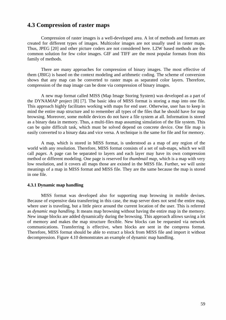
59

4.3 Compression of raster maps

Compression of raster images is a well-developed area. A lot of methods and formats are created for different types of images. Multicolor images are not usually used in raster maps. Thus, JPEG [20] and other picture coders are not considered here. LZW based methods are the common solution for few color images. GIF and TIFF are the most popular formats from this family of methods.

There are many approaches for compression of binary images. The most effective of

them (JBIG) is based on the context modeling and arithmetic coding. The scheme of conversion shows that any map can be converted to raster maps as separated color layers. Therefore, compression of the map image can be done via compression of binary images.

A new map format called MISS (Map Image Storing System) was developed as a part of

the DYNAMAP project [8] [7]. The basic idea of MISS format is storing a map into one file. This approach highly facilitates working with maps for end user. Otherwise, user has to keep in mind the entire map structure and to remember all types of the files that he should have for map browsing. Moreover, some mobile devices do not have a file system at all. Information is stored as a binary data in memory. Thus, a multi-files map assuming simulation of the file system. This can be quite difficult task, which must be solved depend on concrete device. One file map is easily converted to a binary data and vice versa. A technique is the same for file and for memory.

A map, which is stored in MISS format, is understood as a map of any region of the

world with any resolution. Therefore, MISS format consists of a set of sub-maps, which we will call pages. A page can be separated to layers and each layer may have its own compression method or different modeling. One page is reserved for thumbnail map, which is a map with very low resolution, and it covers all maps those are existed in the MISS file. Further, we will unite meanings of a map in MISS format and MISS file. They are the same because the map is stored in one file. 4.3.1 Dynamic map handling

MISS format was developed also for supporting map browsing in mobile devises. Because of expensive data transferring in this case, the map server does not send the entire map, where user is traveling, but a little piece around the current location of the user. This is referred as dynamic map handling. It means map browsing without having the entire map in the memory. New image blocks are added dynamically during the browsing. This approach allows saving a lot of memory and makes the map structure flexible. New blocks can be requested via network communications. Transferring is effective, when blocks are sent in the compress format. Therefore, MISS format should be able to extract a block from MISS file and import it without decompression. Figure 4.10 demonstrates an example of dynamic map handling.

60

Figure 4.10: Dynamic map handling.

Separation to blocks is defined before attaching a layer into the map. Then, blocks are numbered as shown in Figure 4.11. Thus, a layer stores a block not as a part of the image, but as a binary data with appropriate index. Notice, that a layer does not necessary contain an integer number of blocks in the image width and in the image height.

1 32 4

65 87 9

1110 1312 14

1615 1817 19

2120 2322 24

0

Figure 4.11: Image blocks numbering. 4.3.2 MISS map as a hierarchical structure

Finally, we got MISS map as a hierarchy structure as shown in Figure 4.12. The map consists of the thumbnail page and a set of pages. A page consists of geographic information, a page resolution, a background color and a set of layers. Each layer has its own filename for decompression, color, shifting in the map (usual equals zero), separation to blocks, additional data for decompression and an array of blocks. Additional data for decompression denotes a model for semi-adaptive methods as described [7]. This information is inside the layer because each layer can have its own method of compression and parameters of the model. A block is a

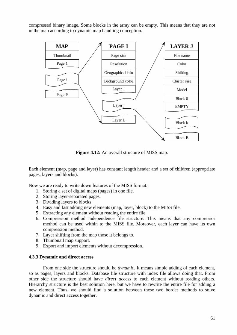
61

compressed binary image. Some blocks in the array can be empty. This means that they are not in the map according to dynamic map handling conception.

MAP

Thumbnail

Page 1

Page P

Page i

PAGE I

Page size

Resolution

Geographical info

Background color

Layer 1

Layer L

Layer j

LAYER J

File name

Color

Shifting

Cluster size

EMPTY

Block B

Block k

Model

Block 0

Figure 4.12: An overall structure of MISS map. Each element (map, page and layer) has constant length header and a set of children (appropriate pages, layers and blocks). Now we are ready to write down features of the MISS format.

1. Storing a set of digital maps (pages) in one file. 2. Storing layer-separated pages. 3. Dividing layers to blocks. 4. Easy and fast adding new elements (map, layer, block) to the MISS file. 5. Extracting any element without reading the entire file. 6. Compression method independence file structure. This means that any compressor

method can be used within to the MISS file. Moreover, each layer can have its own compression method.

7. Layer shifting from the map those it belongs to. 8. Thumbnail map support. 9. Export and import elements without decompression.

4.3.3 Dynamic and direct access

From one side the structure should be dynamic. It means simple adding of each element, so as pages, layers and blocks. Database file structure with index file allows doing that. From other side the structure should have direct access to each element without reading others. Hierarchy structure is the best solution here, but we have to rewrite the entire file for adding a new element. Thus, we should find a solution between these two border methods to solve dynamic and direct access together.

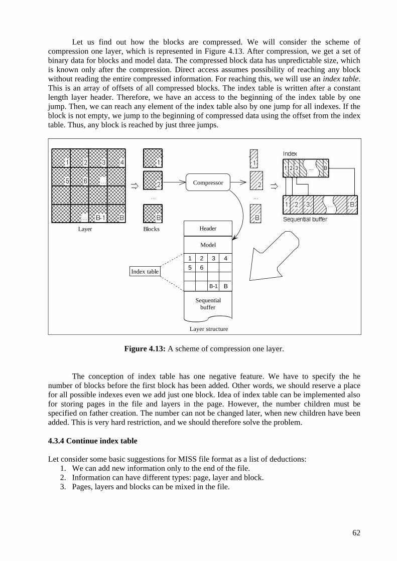
62

Let us find out how the blocks are compressed. We will consider the scheme of compression one layer, which is represented in Figure 4.13. After compression, we get a set of binary data for blocks and model data. The compressed block data has unpredictable size, which is known only after the compression. Direct access assumes possibility of reaching any block without reading the entire compressed information. For reaching this, we will use an index table. This is an array of offsets of all compressed blocks. The index table is written after a constant length layer header. Therefore, we have an access to the beginning of the index table by one jump. Then, we can reach any element of the index table also by one jump for all indexes. If the block is not empty, we jump to the beginning of compressed data using the offset from the index table. Thus, any block is reached by just three jumps.

Layer

Compressor

Blocks

Model

1 2 3 4

5 6

B-1 B

Sequentialbuffer

Layer structure

Header

Index table

Figure 4.13: A scheme of compression one layer.

The conception of index table has one negative feature. We have to specify the he number of blocks before the first block has been added. Other words, we should reserve a place for all possible indexes even we add just one block. Idea of index table can be implemented also for storing pages in the file and layers in the page. However, the number children must be specified on father creation. The number can not be changed later, when new children have been added. This is very hard restriction, and we should therefore solve the problem. 4.3.4 Continue index table Let consider some basic suggestions for MISS file format as a list of deductions:

1. We can add new information only to the end of the file. 2. Information can have different types: page, layer and block. 3. Pages, layers and blocks can be mixed in the file.

63

4. We will add information in hierarchical order. This means that when we add a layer, the page, which the layer belongs to, should exist. The same applies to adding the blocks to the layer.

5. Thus, each page should “know” where all its layers are stored. Therefore, it should have a run length index table for storing offsets of the layers. The same is for the block index table for each layer.

6. Our solution is to use Continue Index Table (CIT). CIT is a special index table with possibility of variant the number of bytes reserved for each index and continue the table at the end of the file. CIT consists of a set of blocks. The first block specifies the number of bytes per index and the number of indexes in one block. Last four bytes of each block are reserved for the offset of the next block of the table. The last block is specified using a special offset 0xFFFF. A structure of the first block is shown in Figure 4.14. Next blocks have the same structure without the first two fields.

Fixed size

Figure 4.14: A structure of the first block of the continue index table.

On the creation, the CIT has two parameters: fixed size and bytes per index. Bytes per index are the number of bytes, which are used for storing each index. This value is stored in the first byte of the CIT. Fixed size is the number of indexes, which are stored in one block. Next two bytes of a CIT are used for storing this value. The space after that is reserved for the fixed size indexes and filled by zeros. The last four bytes are used to storing a relative offset to the next block of the table. If we will change a value of the index in the place from zero to fixed size, the CIT just will change the appropriate bytes. If we will write an index in the place, which is more than fixed size, CIT will automatically continue itself in the end of the file and write the appropriate offset to the next block. Thus, we can add information to file and continue CIT whenever we want. 4.3.5 MISS file structure

Let us now consider the detailed structure of the MISS file a shown in Figure 4.15. It consists of the file header, the pages CIT and mixed page records, layer records and block records. Pages records are reached via pages CIT, layer records via layers CIT of the page, block records via blocks CIT of the layer.

Fixed size (2 bytes)

Index 1

Index 2

Index 3

Index last

Offset of the next table part

Bytes per index (1 byte)

64

Figure 4.15: A structure of the MISS file.

The file header is eight bytes long. Table 4.5 shows the fields of the file header. The page record consists of the page header (31 bytes long) and the layers CIT, which includes the global offsets of the all layers, which are belonged to the page. Table 4.6 shows the fields of the page header. Geographical points are stored using Latitude-Longitude coordinate system. The layer record contains of the layer header and the blocks CIT, which includes the global offset to the all exist blocks belonged to the layer. The layer header has a run length because it includes a run-length model information. Table 4.7 shows the fields of the layer header. The block record contains the data length (4 bytes) of the block and the data. Table 4.8 shows the fields of the block record.

Table 4.5: MISS file header.

Table 4.6: MISS page header.

Position Byte 0 Byte 2 Byte 4 Byte 6

Filed File Code

Version Code Number of Pages

Number of Thumbnail Page

Value 0xFDE2

100 — —

Type ULONG (2) ULONG (2) ULONG (2) ULONG (2)

Position Byte 0 Byte 2 Byte 4 Byte 6 Byte 8 Byte 12 Byte 16 Byte 20 Byte 24 Byte 28

Filed Number of Layers Page Bitmap Width Page Bitmap Height Page Scale (meters per pixel) Page Geo Left Page Geo Top Page Geo Right Page Geo Bottom Page Rotation Page Background Color

Value — — — — — — — — — (R, G, B)

Type ULONG (2) ULONG (2) ULONG (2) ULONG (2) SLONG (4) SLONG (4) SLONG (4) SLONG (4) ULONG (4) ULONG (3)

File Header

Pages CIT

Page Record

Layer Record

Block Record

Layer Record

65

Table 4.7: MISS layer header.

Table 4.8: MISS block header.

Position Byte 0 Byte 40 Byte 43 Byte 47 Byte 51 Byte 55 Byte 59 Byte 63

Filed Layer File Name Layer Color Layer X Shift Layer Y Shift Block Width Block Height Layer Data Length (LDL) Layer Data

Value — (R, G, B) — — — — — —

Type Char [40] ULONG (3) SLONG (4) SLONG (4) ULONG (4) ULONG (4) ULONG (4) BYTE [LDL]

Position Byte 0 Byte 4

Filed Block Data Length (CDL) Block Data

Value — —

Type ULONG (4) BYTE [CDL]

66

Chapter 5 Experiments

The chapter considers experiments of rasterization and compression of real maps. Appropriate software was created using ideas and algorithms from the two previous chapters. We will consider time and size characteristics of rasterization and compression and show that MISS format allows achieving very good results.

67

This part is dedicated to statistic information for conversion from vector maps (ArcShape and SVF formats) to the compressed raster representation (MISS format). First of all, we should point that comparing raster and vector maps is not easy because of different type of information in these formats. The main difference is the scaling. Vector map scaling does not affect the quality of the map a lot. The same raster map must consist of a set of images because scaling of a raster map highly decreases its quality (see Figure 3.1). Here we assume that six different images are enough for good scaling.

Conversion from a vector format to the MISS format contains of two stages: the first one is conversion from the vector map to the project file and to the set of binary images. Each binary image represents one layer. Using the project file, another program compresses the map to the MISS format. We will use MISS format with context modeling compression and arithmetic coding.

Let us consider an ArcShape map first. The big map (10x10 kilometers) in NSL format

was taken for the experiment. Section 3.2 shows that parameters of conversion are resolution and layer separation. Resolution depends on six map scales, which we will take for the experiment. The map consists of four layers. The layer separation is done using a color feature of the primitives:

1. Fields (yellow), 2. Water (blue), 3. Elevation lines (brown) 4. Basic (black).

Background color is not specified in ArcShape maps. Assuming they have white

background color. Thus, after rasterization we will get four binary files and the project file. The project file is created according to specification form Section 3.2 and illustrated in Figure 5.1.

# Map project Input=E:\Veis\Maps\m431204Ap.shp Output=431204 Background=16777215 XSize=5000 YSize=5000 LeftBottomX=33.745360 LeftBottomY=64.258233 RightTopX=33.785290 RightTopY=64.388223 Scale=2.000000 Rotation=0.000000 # Layer section # Layers: # LayerNumber=LayerName, LayerType, DependentFrom Layer0=431204_0.pbm, 0, 0 Layer1=431204_1.pbm, 0, 1 Layer2=431204_2.pbm, 0, 2 Layer3=431204_3.pbm, 0, 3 # Color section # LayerNumber=Color Color0=255,255,168 Color1=168,255,255 Color2=230,153,0

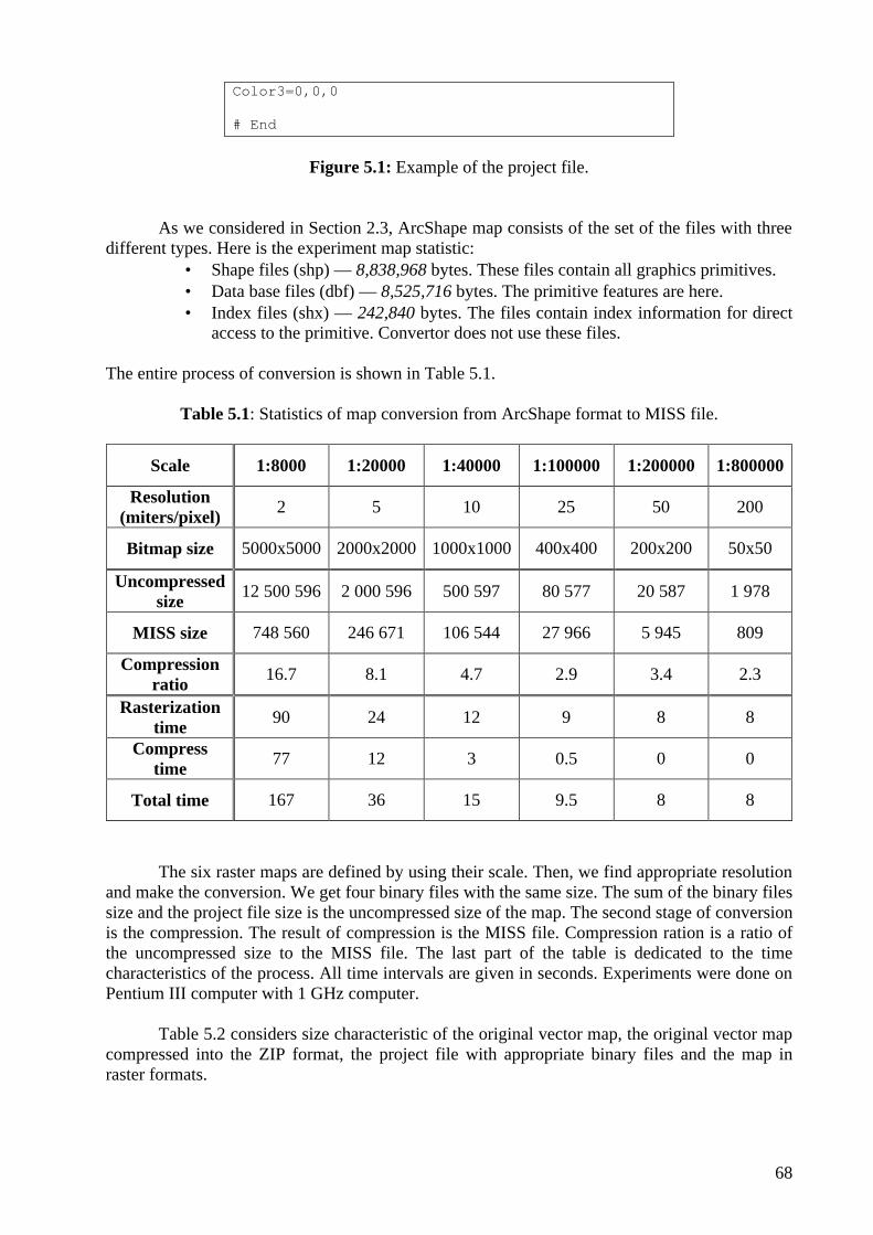
68

Color3=0,0,0 # End

Figure 5.1: Example of the project file.

As we considered in Section 2.3, ArcShape map consists of the set of the files with three different types. Here is the experiment map statistic:

• Shape files (shp) — 8,838,968 bytes. These files contain all graphics primitives. • Data base files (dbf) — 8,525,716 bytes. The primitive features are here. • Index files (shx) — 242,840 bytes. The files contain index information for direct

access to the primitive. Convertor does not use these files. The entire process of conversion is shown in Table 5.1.

Table 5.1: Statistics of map conversion from ArcShape format to MISS file.

Scale 1:8000 1:20000 1:40000 1:100000 1:200000 1:800000

Resolution (miters/pixel) 2 5 10 25 50 200

Bitmap size 5000x5000 2000x2000 1000x1000 400x400 200x200 50x50

Uncompressed size 12 500 596 2 000 596 500 597 80 577 20 587 1 978

MISS size 748 560 246 671 106 544 27 966 5 945 809

Compression ratio 16.7 8.1 4.7 2.9 3.4 2.3

Rasterization time 90 24 12 9 8 8

Compress time 77 12 3 0.5 0 0

Total time 167 36 15 9.5 8 8

The six raster maps are defined by using their scale. Then, we find appropriate resolution and make the conversion. We get four binary files with the same size. The sum of the binary files size and the project file size is the uncompressed size of the map. The second stage of conversion is the compression. The result of compression is the MISS file. Compression ration is a ratio of the uncompressed size to the MISS file. The last part of the table is dedicated to the time characteristics of the process. All time intervals are given in seconds. Experiments were done on Pentium III computer with 1 GHz computer.

Table 5.2 considers size characteristic of the original vector map, the original vector map

compressed into the ZIP format, the project file with appropriate binary files and the map in raster formats.

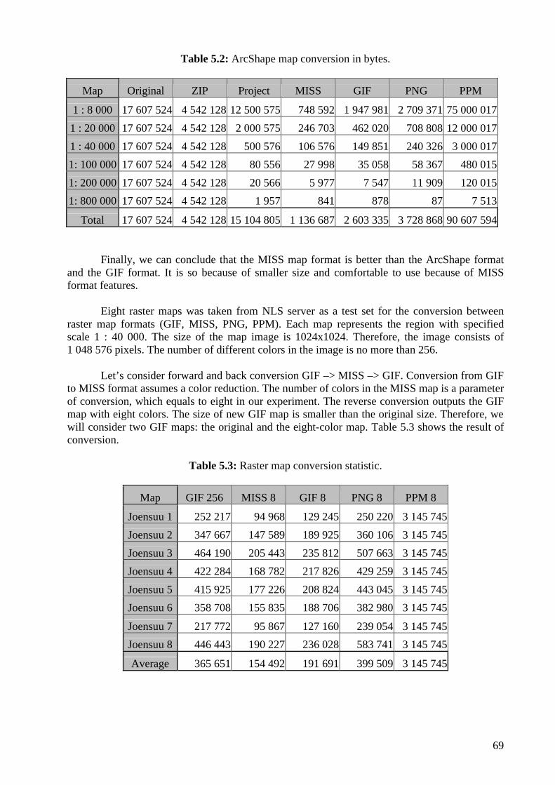
69

Table 5.2: ArcShape map conversion in bytes.

Map Original ZIP Project MISS GIF PNG PPM

1 : 8 000 17 607 524 4 542 128 12 500 575 748 592 1 947 981 2 709 371 75 000 017

1 : 20 000 17 607 524 4 542 128 2 000 575 246 703 462 020 708 808 12 000 017

1 : 40 000 17 607 524 4 542 128 500 576 106 576 149 851 240 326 3 000 017

1: 100 000 17 607 524 4 542 128 80 556 27 998 35 058 58 367 480 015

1: 200 000 17 607 524 4 542 128 20 566 5 977 7 547 11 909 120 015

1: 800 000 17 607 524 4 542 128 1 957 841 878 87 7 513

Total 17 607 524 4 542 128 15 104 805 1 136 687 2 603 335 3 728 868 90 607 594

Finally, we can conclude that the MISS map format is better than the ArcShape format and the GIF format. It is so because of smaller size and comfortable to use because of MISS format features.

Eight raster maps was taken from NLS server as a test set for the conversion between raster map formats (GIF, MISS, PNG, PPM). Each map represents the region with specified scale 1 : 40 000. The size of the map image is 1024x1024. Therefore, the image consists of 1 048 576 pixels. The number of different colors in the image is no more than 256.

Let’s consider forward and back conversion GIF –> MISS –> GIF. Conversion from GIF

to MISS format assumes a color reduction. The number of colors in the MISS map is a parameter of conversion, which equals to eight in our experiment. The reverse conversion outputs the GIF map with eight colors. The size of new GIF map is smaller than the original size. Therefore, we will consider two GIF maps: the original and the eight-color map. Table 5.3 shows the result of conversion.

Table 5.3: Raster map conversion statistic.

Map GIF 256 MISS 8 GIF 8 PNG 8 PPM 8

Joensuu 1 252 217 94 968 129 245 250 220 3 145 745

Joensuu 2 347 667 147 589 189 925 360 106 3 145 745

Joensuu 3 464 190 205 443 235 812 507 663 3 145 745

Joensuu 4 422 284 168 782 217 826 429 259 3 145 745

Joensuu 5 415 925 177 226 208 824 443 045 3 145 745

Joensuu 6 358 708 155 835 188 706 382 980 3 145 745

Joensuu 7 217 772 95 867 127 160 239 054 3 145 745

Joensuu 8 446 443 190 227 236 028 583 741 3 145 745

Average 365 651 154 492 191 691 399 509 3 145 745

70

We can see that MISS format is again better than PNG and GIF formats. The numerical experiments make clear a goal of rasterization and conversion to MISS format. We save a lot of disk space and get a map in very comfortable format. The experiments will help in comparing different map formats.

71

Chapter 6 Conclusions

The chapter is dedicated to comparing map formats, which we considered above. Comparison demonstrates areas of using each format and gives a topic of future research.

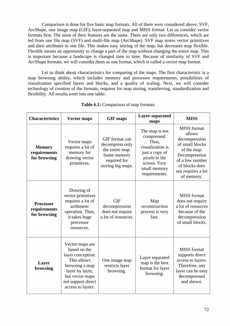
72

Comparison is done for five basic map formats. All of them were considered above: SVF, ArcShape, one image map (GIF), layer-separated map and MISS format. Let us consider vector formats first. The most of their features are the same. There are only two differences, which are led from one file map (SVF) and multi-file map (ArcShape). SVF map stores vector primitives and their attributes in one file. This makes easy storing of the map, but decreases map flexible. Flexible means an opportunity to change a part of the map without changing the entire map. This is important because a landscape is changed time to time. Because of similarity of SVF and ArcShape formats, we will consider them as one format, which is called a vector map format.

Let us think about characteristics for comparing of the maps. The first characteristic is a

map browsing ability, which includes memory and processor requirements, possibilities of visualization specified layers and blocks, and a quality of scaling. Next, we will consider technology of creation of the formats, requires for map storing, transferring, standardization and flexibility. All results went into one table:

Table 6.1: Comparison of map formats.

Characteristics Vector maps GIF maps Layer-separated maps MISS

Memory requirements for browsing

Vector maps requires a lot of

memory for drawing vector

primitives.

GIF format can decompress only the entire map. Some memory

required for storing big maps.

The map is not compressed.

Thus, visualization is just a copy of pixels to the screen. Very

small memory requirements.

MISS format allows

decompression of small blocks

of the map. Decompression of a few number of blocks does

not requires a lot of memory.

Processor requirements for browsing

Drawing of vector primitives requires a lot of

arithmetic operation. Thus,

it takes huge processor resources.

GIF decompression does not require

a lot of resources.

Map reconstruction process is very

fast.

MISS format does not require a lot of resources

because of the decompression of small blocks.

Layer browsing

Vector maps are based on the

layer conception. This allows

browsing a map layer by layer,

but vector maps not support direct access to layers.

One image map restricts layer

browsing.

Layer separated map is the best format for layer

browsing.

MISS format supports direct

access to layers. Therefore, any

layer can be easy decompressed

and shown.

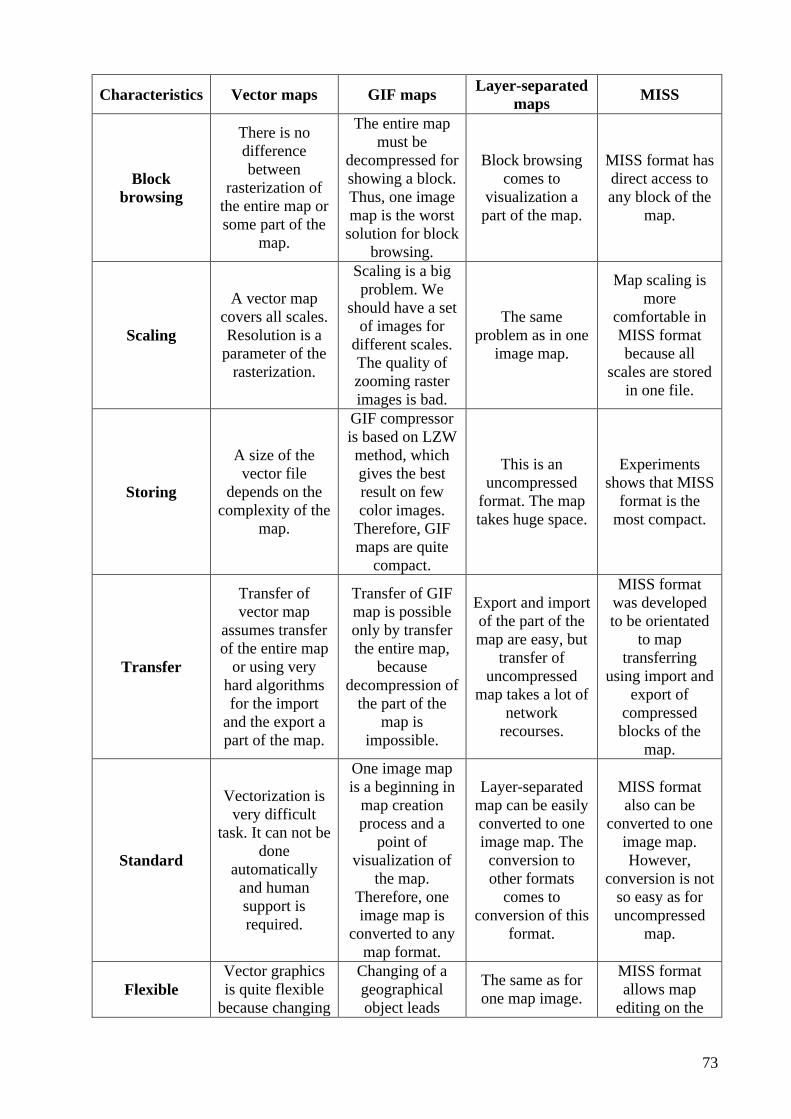
73

Characteristics Vector maps GIF maps Layer-separated maps MISS

Block browsing

There is no difference between

rasterization of the entire map or some part of the

map.

The entire map must be

decompressed for showing a block. Thus, one image map is the worst

solution for block browsing.

Block browsing comes to

visualization a part of the map.

MISS format has direct access to any block of the

map.

Scaling

A vector map covers all scales. Resolution is a

parameter of the rasterization.

Scaling is a big problem. We

should have a set of images for

different scales. The quality of zooming raster images is bad.

The same problem as in one

image map.

Map scaling is more

comfortable in MISS format because all

scales are stored in one file.

Storing

A size of the vector file

depends on the complexity of the

map.

GIF compressor is based on LZW method, which gives the best result on few color images.

Therefore, GIF maps are quite

compact.

This is an uncompressed

format. The map takes huge space.

Experiments shows that MISS

format is the most compact.

Transfer

Transfer of vector map

assumes transfer of the entire map

or using very hard algorithms for the import

and the export a part of the map.

Transfer of GIF map is possible only by transfer the entire map,

because decompression of

the part of the map is

impossible.

Export and import of the part of the map are easy, but

transfer of uncompressed

map takes a lot of network

recourses.

MISS format was developed to be orientated

to map transferring

using import and export of

compressed blocks of the

map.

Standard

Vectorization is very difficult

task. It can not be done

automatically and human support is required.

One image map is a beginning in

map creation process and a

point of visualization of

the map. Therefore, one image map is

converted to any map format.

Layer-separated map can be easily converted to one image map. The

conversion to other formats

comes to conversion of this

format.

MISS format also can be

converted to one image map. However,

conversion is not so easy as for uncompressed

map.

Flexible Vector graphics is quite flexible

because changing

Changing of a geographical object leads

The same as for one map image.

MISS format allows map

editing on the

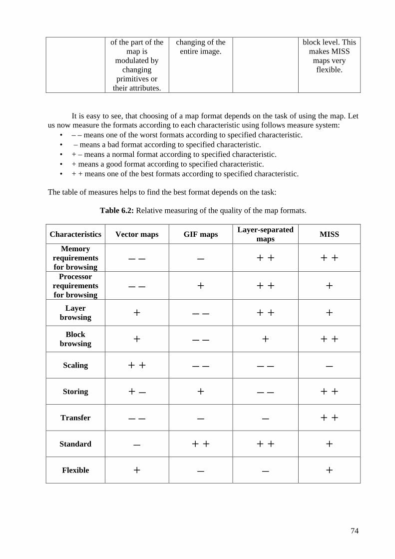
74

of the part of the map is

modulated by changing

primitives or their attributes.

changing of the entire image.

block level. This makes MISS maps very flexible.

It is easy to see, that choosing of a map format depends on the task of using the map. Let

us now measure the formats according to each characteristic using follows measure system: • – – means one of the worst formats according to specified characteristic. • – means a bad format according to specified characteristic. • + – means a normal format according to specified characteristic. • + means a good format according to specified characteristic. • + + means one of the best formats according to specified characteristic.

The table of measures helps to find the best format depends on the task:

Table 6.2: Relative measuring of the quality of the map formats.

Characteristics Vector maps GIF maps Layer-separated maps MISS

Memory requirements for browsing

– – – + + + + Processor

requirements for browsing

– – + + + +

Layer browsing + – – + + +

Block browsing + – – + + +

Scaling + + – – – – –

Storing + – + – – + +

Transfer – – – – + +

Standard – + + + + +

Flexible + – – +

75

Here we can see, that vector maps is good for storing big databases of the maps, one image map is nice in systems, which deal with the entire map. Layer-separated map is a transitional stage of conversion between different formats. MISS format is the best solution for providing a map service for mobile devices.

Mixing of vector and raster formats can burn a new format, which will take the best sides

of all formats. This is a topic of future research.

76

References [1] E. Arge and M. Daeham, “Data reduction of piecewise linear curves”, Technical report,

SINTEFF Informatics, Oslo, Norway, 1994. [2] P. Bourke, “Hershey Vector Font”, 1997.

http://astronomy.swin.edu.au/pbourke/other/hershey/ [3] D. H. Douglas and T. K. Peucker, “Algorithms for reduction of the number of points

required to represent a digitized line or its caricature”, The Canadian Cartographer, 10/2, pp 112–122, 1973.

[4] L. Dumaine, “Vector Map Tools Dedicated to Mobile Device Context”, University of

Joseph Fourier, pp 73–77, 2001. [5] G. H. Dutton, “A Hierarchical Coordinate System for Geoprocessing and Cartography”,

Springer-Verlag Berlin Heidelberg, 1999. [6] ESRI, “ESRI Shapefile Technical Description”, An ESRI White Paper, 1998.

http://www.esri.com/library/whitepapers/pdfs/shapefile.pdf [7] P. Fränti, E. Ageenko, P. Kopylov, S. Gröhn and F. Berger, “Compression of map images

for real-time applications”, Research Report A-2001-1, University of Joensuu, Department of Computer Science, 2001.

[8] P. Fränti, DYNAMAP Project, University of Joensuu, Department of Computer Science,

2001. http://cs.joensuu.fi/pages/franti/dynamap/

[9] P. Fränti, “Image Compression”, Lecture Notes, University of Joensuu, Department of

Computer Science, 2000. [10] P. Fränti, “Image Processing”, Lecture Notes, University of Joensuu, Department of

Computer Science, pp 6–12, 2001. [11] D. Huffman, “A Method for the Reconstruction of Minimum Redundancy Codes”, Proc.

of the IRE, Vol. 40, pp 1098-1101, 1952. [12] JBIG. ISO/IEC International Standard 11544 (1993) ISO/IEC/JTC1/SC29/WG9; also

IYU-T Recommendation T.82, Progressive Bi-level Image Compression. [13] A.N. Kolesnikov, V.I. Belekhov, I.O. Chalenko, "Vectorization of the raster images”,

Pattern Recognition and Image Analysis, 1996, vol. 6, No. 1, 4. [14] A. Kolesnikov and P. Fränti, “Reduced-search dynamic programming for approximation

of polygonal curves”, Research Report A-2001-4, University of Joensuu, Department of Computer Science, 2001.

77

[15] L. C. Mai, “Introduction to Computer Vision and Image Processing”, Department of Pattern Recognition and Knowledge Engineering Institute of Information Technology, Hanoi, Vietnam, Section 6.3. http://203.162.7.85/unescocourse/computervision/computer.htm

[16] J. Miano, “Compression image file formats”, ACM Press, 1999. [17] M. Nelson, “The data compression book”, IDG Books Worldwide, Inc, 1995. [18] NLS, “Technical description of NLS map format”.

http://www.nls.fi/kartta/selosteet/ts/maastotietokanta.html [19] M. Ollikainen, “The Finnish National Grid Coordinate System”, NLS.

http://www.nls.fi/kartta/julkaisu/kkj.html [20] W.B. Pennebaker, J.L. Mitchell, “JPEG Still Image Data Compression Standard”, Van

Nostrand Reinhold, 1993. [21] D. Plant, “What's a Bezier Curve?”, 1996.

http://www.moshplant.com/direct-or/bezier/ [22] J. Rissanen, G.G. Langdon, “Arithmetic Coding”, IBM Journal of Research and

Development, Vol. 23 (2), pp 149-162, March 1979. [23] Soft Source, “Information on SVF (Simple Vector Format)”

http://www.softsource.com/svf/ [24] V. Veis and S. Nevalainen, ”Convertor”, IT Project, University of Joensuu, Department

of Computer Science, 2001. [25] M. Zeiler, “Modeling Our World”, ESRI, 1999. [26] J. Ziv and A. Lempel, “A compression of individual sequences via variable-rate coding”,

IEEE Transactions on Information Theory, Volume 24, Number 5, pp 530–536, September 1978.

[27] J. Ziv and A. Lempel, “A universal algorithm for sequential data compression,” IEEE

Transactions on Information Theory, Volume 23, Number 3, pp 337–343, May 1977.