Repositioning Dynamics and Pricing Strategy∗

Paul B. EllicksonUniversity of Rochester

Sanjog MisraUCLA

Harikesh S. NairStanford University

September 10, 2012

Abstract

We measure the revenue and cost implications to supermarkets of changing their price posi-tioning strategy in oligopolistic downstream retail markets. Our approach formally incorporatesthe dynamics induced by the repositioning in a model with strategic interaction. We exploit aunique dataset containing the price-format decisions of all U.S. supermarkets in the 1990s. Thedata contain the format-change decisions of supermarkets in response to a large shock to theirlocal market positions: the entry of Wal-Mart. We exploit the responses of retailers to Wal-Mart entry to infer the cost of changing pricing-formats using a “revealed-preference”argumentsimilar in spirit to Bresnahan and Reiss (1991). The interaction between retailers and Wal-Martin each market is modeled as a dynamic game. We find evidence that entry by Wal-Mart had asignificant impact on the costs and incidence of switching pricing strategy. Our results add tothe marketing literature on the organization of retail markets, and have implications for long-run market structure in the supermarket industry. Our approach, which incorporates long-rundynamic consequences, strategic interaction, and sunk investment costs, may be used to modelempirically firms’positioning decisions in Marketing, more generally.Keywords: Positioning, dynamic games, EDLP, PROMO, pricing, supermarkets, Wal-Mart.

∗First version, January 2011. We would like to thank the review team, Robert Miller, and Ariel Pakes, as wellas seminar participants at Carnegie-Mellon, UCLA, and the 2011 Marketing-Industrial Organization, SICS, andMarketing Science conferences for many helpful comments. The usual disclaimer applies.

1

1 Introduction

Large changes to some or all of a firm’s Marketing apparatus are referred to as “repositioning.”

While common in product markets and extensively discussed in management textbooks (e.g., Ries

and Trout (1981)), empirical analysis of repositioning decisions in the academic literature has re-

mained scarce. Perhaps the most visible forms of repositioning are brand related. Recent examples

include Domino Pizza’s attempt to switch their reputation from fast delivery to high quality, and

the repositioning of UPS from shipping to full offi ce solutions. Other examples include adjust-

ments to product lines, such as Hyundai’s recent move into the luxury auto segment in the U.S.

or Kodak’s long-delayed transition to digital imaging. While brand related changes are common,

they are far from the only examples. Apple’s inclusion of third party retailers can be thought

of as repositioning their downstream distribution strategy, while Proctor and Gamble’s adoption

of “Value-Based Pricing” in 1992 to reduce trade-promotions, was a repositioning of their over-

all pricing strategy (Ailawadi, Lehmann, and Neslin (2001)). St-James (2001) describes several

instances of repositioning by firms in US consumer product markets, including a detailed history

from the 1920s of attempts by Sears, Wards and J.C. Penny chain stores to periodically reposition

themselves in response to changing consumer tastes and competition.

Repositioning is different from new entry as it is inherently history-dependent: repositioning

typically requires incurring costs to undo past product related decisions. Therefore, repositioning

costs to incumbents can often be much larger than the cost of entry to new firms. Repositioning

frequently involves complex investments needed to overcome within-firm managerial resistance to

change, to rework channel relationships, and to educate (and advertise to) consumers about the

new positioning, all investments that are large and sunk. The magnitude of repositioning costs

have substantive implications for competition and market structure. Low repositioning costs help

constrain market power by enabling competitors to react faster to changes in a firm’s product-lines

and product attributes. When repositioning investments are sunk, they also have commitment

value (Dixit and Pindyck (1994)), implying current repositioning decisions can affect long-run

market outcomes such as the future entry and exit behavior of rival firms. Hence, measuring

repositioning costs are important to understanding the economic underpinnings of market structure

2

in an industry.

In this paper we examine the repositioning of the pricing strategies of U.S. supermarket firms.

Our empirical goals are to measure the revenue and cost implications to supermarkets of changing

their store-level pricing formats. These pricing formats are broadly split between EDLP (Every

Day Low Price) and PROMO (or promotional) strategies.1 EDLP stores charge a low regular

price per product with little temporal price variation, while PROMO stores are characterized by

higher regular prices, punctuated by frequent price promotions or “sales.”A store’s choice between

EDLP or PROMO is motivated by both demand- and cost-side considerations. On the demand

side, choosing PROMO over EDLP offers an opportunity for supermarkets to intertemporally price

discriminate, by using price cycles to sell differentially to consumers of varying price information,

loyalty, stockpiling costs or valuations (Varian (1980); Salop and Stiglitz (1982); Sobel (1984); Lal

and Rao (1997); Pesendorfer (2002); Bell and Hilber (2006)). Further, the frequent price variation

under PROMO may create an option value to consumers of visiting the store more frequently by

reducing their average basket size per trip (Bell and Lattin (1998); Ho, Tang, and Bell (1998)). On

the cost-side, EDLP enables retailers to reduce inventory costs, to better coordinate supply-chains,

and to reduce stock-out risk by smoothing the demand variability induced by frequent sales. The

choice of EDLP or PROMO is an important strategic choice faced by retailers that affects their

price image, with significant long-term implications for profitability and local market structure (Lal

and Rao (1997); Ellickson and Misra (2008)).

Several factors may cause a supermarket chain to change its store pricing format in a local mar-

ket. One first-order factor is response to competitive entry, especially by rivals with a comparative

advantage in a particular strategy. Our data, which covers a census of supermarket entry, exit,

revenue and format choices in the 1990s, includes a period of intense readjustment in response to

a one such event: the introduction of Wal-Mart supercenters, which exclusively follow an EDLP

strategy. The entries of Wal-Mart supercenters serve as large shocks to the competitive structure

of local markets, inducing a large number of format switches and a host of exits. Our identification

of repositioning costs exploits these switches heavily, and rests on a revealed preference argument

1PROMO is also referred to as “HiLo.”

3

similar to that of Bresnahan and Reiss (1991) and Bresnahan and Reiss (1994): if we see that a firm

switched its price positioning, it has to be that the profits (in a present-discounted sense) from the

switch were higher than those without it. As we observe revenues, we can further decompose this

restriction on profits into a restriction on the costs of the change. Combining this with a structural

model of the industry and variation across markets enables us to relate these restrictions to specific

market and competitive factors. Identification derives from observing both switches to a different

price positioning and exits. Intuitively, if repositioning costs were zero, a firm whose revenues do

not cover fixed costs under its current pricing strategy could costlessly shift to an alternative pricing

strategy with higher net payoffs. Observing another firm stay in the market under the alternative

pricing strategy reveals that the net payoffs for this alternative are positive. Observing, at the

same time, that the focal firm is exiting, and not switching, thus indicates that the repositioning

costs of switching to the alternative strategy are large.

Additional identification derives from the joint distribution of entry, stays, switches, exits, and

revenues observed across markets. The level of present-discounted revenues required to make N

incumbents switch to a pricing strategy versus that required to make N entrants choose that

strategy, identifies the extent to which the repositioning costs are higher than entry costs. The

level of present-discounted revenues required to make N entrants choose a pricing strategy versus

required to make N incumbents who currently operate under that strategy to exit, identifies the

extent to which the repositioning costs are sunk.

We then combine this identification strategy with a model of format choice to decompose the

effect of repositioning into revenue and cost components. This decomposition is informative to the

underlying choice problem. On the revenue side, for example, a move from PROMO to EDLP

implies a loss to the supermarket in its price discrimination ability as discussed above, as well as

demand losses from potential consumer antagonism to changes in pricing policies (Anderson and

Simester (2010)). On the cost side, much of costs associated with advertising the new positioning;

with the man-hours involved in updating inventory and supply-chain systems for changing pricing

strategy; and with purchase of new pricing and demand-management software to manage promo-

tional activity, are sunk. As the demand-side effects are long-run, and the cost-side investments are

4

sunk, these cost-benefit trade-offs involve dynamic considerations. Further, strategic interaction

from other supermarkets are likely important. Most retail markets in the US tend to be concen-

trated, with a few (3-5) dominant players controlling the market, irrespective of its size (Ellickson

(2007)), implying firms face oligopolistic competition at the local market level.

Accommodating these key considerations, we utilize an empirical framework that treats format

change as a dynamic problem with sunk investment. Strategic interactions are accommodated by

formulating the model as a dynamic game of incomplete information with entry and exit, in the

spirit of Ericson and Pakes (1995). Using the identification strategy presented above, we propose

new ways to infer the structural parameters of the game by exploiting recently developed methods

for two-step estimation of dynamic games (Aguirregabiria and Mira (2007); Arcidiacono and Miller

(2012)). We also show how to incorporate revenue information (a continuous outcome) into the

estimation procedure in an internally consistent manner, while accounting for the dynamic selection

induced by the co-determination of these with the discrete-choices, by extending the methods

proposed by Ellickson and Misra (2012) to a dynamic environment. The incorporation of strategic

interaction is important to the estimation of repositioning costs. For instance, in a competitive

market, a supermarket may be reluctant to switch from PROMO to EDLP because it anticipates

that price competition may be toughened if a rival firm, currently doing PROMO, also shifts to

EDLP in response to its action. In the absence of this control, the persistence induced on pricing

strategy (and observed in the data) by such strategic interaction would be falsely interpreted as

due to repositioning costs. This is the main additional complication that arises when measuring

switching costs for firms as opposed to consumers. This is accommodated in our framework by

allowing firms to form beliefs about the reactions of their rivals, which then influence their choice

of pricing formats. In our Markov Perfect equilibrium, beliefs and actions are consistent, and will

be functions of the state variables faced by the firm. We are thus able to recover the beliefs of the

firms directly from the data for use in estimation, by semiparametrically projecting the observed

actions of the firms onto the relevant state vector.

Our results imply the cost and revenue effects of changing pricing formats are large and asym-

metric. In particular, for the median store in our data, a change from EDLP to PROMO requires

5

a fixed outlay of about $2.3M borne over a 4 year horizon. On the other hand, a switch from

PROMO to EDLP requires outlays about 6 times as large, providing a clear explanation for why

EDLP was never uniformly adopted − it is simply too expensive to be viable in most markets. We

also find evidence for significant heterogeneity in these costs across markets, holding out scope for

geographic segmentation in a given chain’s price positioning strategies. Consistent with existing

evidence (cited below), we find overwhelming evidence that PROMO produces higher revenues. For

the median store-market, PROMO yields an incremental revenue of about $6.2M annually relative

to EDLP. We also find that the entry of Wal-Mart has large and significant effects on the propen-

sity to switch pricing formats. It also has a disproportionately asymmetric effect on supermarket

revenues, with its entry hurting revenues of EDLP stores about twice as much as it does PROMO

stores (reducing revenues by $1.47M compared to $0.69M annually at the median).

Substantively, empirical evidence on the relative attractiveness of EDLP versus PROMO strate-

gies is scarce. In a study from one retailer, Mulhern and Leone (1990) report sales increased in a

switch from EDLP to PROMO. In the strongest evidence available so far, randomized pricing exper-

iments involving the Dominick’s stores conducted by the University of Chicago (Hoch, Dreze, and

Purk (1994)) find that category by category EDLP is not preferred relative to PROMO (revenues

declined when categories, but not stores, were switched from PROMO to EDLP). The literature is

still lacking a clear accounting of how these trade-offs change when the long-term economic costs

of switching are incorporated. In our data, we find that a switch from EDLP to PROMO increases

revenues as well as the probability of store-exits, suggesting that format change cost considerations

are qualitatively important to an audit of price positioning strategies.

Our approach is closest in structure to Sweeting (2011), who estimates the dynamic costs radio

stations face when changing music formats. Substantively, the question we ask is different as

there is no role for consumer pricing in radio (since radio music is free); further, compared to

his model, we accommodate new entry and allow incumbent firms to exit, which drives part of

the identification. In our model, the margin from staying in the market versus exiting identifies

the per-period fixed costs of operation; while the margin from changing a format, conditional on

staying in the market, identifies format-switching costs. Our paper is also broadly related to an

6

empirical literature that has documented descriptively the effects of Wal-Mart entry on incumbent

firms (e.g. Singh, Hansen, and Blattberg (2006); Basker and Noel (2009); Matsa (2011); Ellickson

and Grieco (2011)); to a recent empirical literature in Marketing of applying static discrete games

to entry models of supermarket supply (Orhun (2006); Vitorino (2007); Zhu and Singh (2009));

and to an ambitious recent structural literature that has modeled the entry decisions of Wal-Mart

as dynamic (but abstracting from strategic interactions; Holmes (2011)), or as jointly determined

across geographies (but abstracting from dynamics as in Jia (2008) or Ellickson, Houghton, and

Timmins (2010)). Our focus on measuring dynamic switching costs for firms complements the recent

literature in Marketing that has considered dynamics induced by consumer-side switching costs for

demand (Hartmann and Viard (2008); Goettler and Clay (2011)) and for firm’s pricing decisions

(Dube, Hitsch, and Rossi (2009)). Our empirical exercise can also be thought of as measuring

an adjustment cost of changing pricing strategy, and is broadly related to the empirical literature

measuring the costs to retailers of changing prices (e.g., Levy, Bergen, Dutta, and Venable (1997);

Slade (1998)).

More generally, we emphasize that repositioning is fundamentally a dynamic decision due to

both the sunk nature of repositioning investments, and because current repositioning decisions

affect future demand and competitive reactions. Hence, repositioning decisions in Marketing and

Industrial Organization should formally be thought of as dynamic games. Here, we illustrate

how viewing product markets through this lens enables us to parsimoniously accommodate these

dynamic considerations and to structurally estimate the benefits and costs of repositioning in real

market settings.

The paper is organized as follows. Section 2 provides background on the supermarket industry,

as it appeared in the late 1990s, describes the dataset, establishes key stylized facts, and details

our approach to identification. Section 3 introduces our formal model of retail competition, while

section 4 outlines our empirical strategy and econometric assumptions. Section 5 contains our main

empirical results, along with a discussion of their broader implications. Section 6 concludes.

7

2 Industry, Data and Stylized Facts

Our data relates to the 1990s, a period of significant change for the U.S. supermarket industry.

Conventional supermarket chains faced intense competition from the rise of new store formats and

innovative entrants including Club Stores (like Sam’s Club and Costco) and limited assortment

chains, (such as Aldi and Save-A-Lot). At the forefront was Wal-Mart, which built its first su-

percenter (a combination discount store and grocery outlet) in 1988, opened its 200th outlet in

1995, and would operate over 1000 supercenters by 2001. The basis of the competitive threat from

entry lay in the perception that limited service, thinner assortments and “every day low pricing”

created enormous cost savings and increased credibility with consumers. EDLP, together with a

limited product assortment, offered the promise of more predictable demand, reduced inventory

and carrying costs, fewer advertising expenses, and lower menu and labor costs. Larger scale was

thought to go hand in hand with lower prices. Much of this perception was driven by the success

of Wal-Mart alone, which leveraged technical sophistication in IT with buying power to squeeze

suppliers and tighten margins, staking out a dominant position in the retailing sector and forging

an indelible perception as a low-cost leader. Many of the strategic decisions made by the incumbent

supermarket chains were geared toward competition with Wal-Mart. A more detailed discussion of

reports in the trade-press regarding supermarket’s response to Wal-Mart entry and their choice of

EDLP or PROMO in response to that entry is available on request from the authors.

While the impact of Wal-Mart on retail competition is undisputed, many observers assumed

that the EDLP format would also come to dominate the supermarket landscape, ignoring both the

significant sunk investments in repositioning necessary to implement it and the offsetting benefits

of having frequent promotions. While Wal-Mart has continued its growth in the supermarket

industry, we now know the EDLP revolution did not come to pass. Our empirical analysis is aimed

at understanding why. To do so, we seek to decompose the returns to adopting the EDLP or

PROMO format into three components: revenues, operating costs, and repositioning costs. We

find that while EDLP pricing provides significant cost savings, it is very expensive to implement

(i.e. the repositioning costs are significant). Moreover, it leads to a significant reduction in revenues

relative to PROMO pricing.

8

2.1 Data and Descriptive Results

We now describe our dataset, and present some key stylized facts in the data that pin down

switching costs. The data for the supermarket industry are drawn from two primary sources: the

Trade Dimensions TDLinx panel database and the 1994 and 1998 frames of the Supermarkets

Plus Database. Trade Dimensions continuously collects store level data from every supermarket

operating in the U.S. for use in their Marketing Guidebook and Market Scope publications, as well as

selected issues of Progressive Grocer magazine. The data are also sold to consulting firms and food

manufacturers for marketing purposes. The supermarket category is defined using the government

and industry standard: a store selling a full line of food products and generating at least $2 million in

yearly revenues. Foodstores with less than $2 million in revenues are classified as convenience stores

and are not included in the dataset. For the TDLinx panel, Trade Dimensions collects information

on average weekly volume, store size, number of checkouts, and several additional store and chain

level characteristics by surveying store managers and cross-validating their responses with each

store’s principal food broker. We are using the 1994, 1998, and 2002 frames from this panel.

The TDLinx dataset does not contain information on pricing format. The information on pricing

strategy was obtained from a second dataset, the Supermarkets Plus Database, which was only

collected in 1994 and 1998, and contained a more detailed set of characteristics. In particular,

managers were asked to choose the pricing strategy that was closest to what their store practices

on a general basis: either EDLP, PROMO or HYBRID. EDLP was defined as having “Little

reliance on promotional pricing strategies such as temporary price cuts. Prices are consistently low

across the board, throughout all food departments.”PROMO was defined as making “Heavy use

of specials − usually through manufacturer price breaks or special deals.”The HYBRID category

was included for those stores that practiced a combination of the two, presumably across separate

categories or departments. Since we are interested in the adoption of a pure EDLP positioning,

we include HYBRID stores in the PROMO category. For additional information on the dataset

(including a verification of its correlation with actual price variation using independent scanner

data) see Ellickson and Misra (2008).

9

2.1.1 Markets and Market Structure

While there are several retail channels through which to purchase food for at-home consumption

(e.g. supermarkets, mom and pop grocers, specialty markets, convenience stores, club stores) we

focus on the supermarket channel exclusively, further narrowing our focus to chain supermarkets

operating within 276 designated U.S. Metropolitan Statistical Areas (MSAs). Following Ellickson

and Misra (2008), which established that strategic pricing decisions have a strong local component,

our unit of observation is a store operating in a local market, taken here to be a zip code.2 Since we

are primarily interested in understanding repositioning choices, which only applies to supermarket

firms (as opposed to Wal-Mart), the following summary statistics and descriptive analysis will focus

exclusively on this set of firms. Any exceptions are noted explicitly.

Table 1 provides statistics that describe the local markets and firms. Focusing on the first frame

of the table, we note that the average market contains about 22 thousand consumers, while the

full set ranges in size from unpopulated (i.e. zoned to be purely commercial) to 112 thousand.

There is also substantial variation in both ethnic composition and income levels across markets.

Frames two and three summarize market structure in the two periods for which we have pricing

data. While the average market contains just over 2 stores, some contain as many as 16. About

28% percent of stores in the average market choose EDLP, while the remaining 72% offer PROMO.

The typical number of stores and the fraction choosing EDLP are both relatively stable over time.

The biggest change observed in the data is the number of markets that either contain a Wal-Mart

or face one in their surrounding MSA. Both numbers increased by a factor of 5 over this four year

period, reflecting the dramatic roll out of the supercenter format that occurred at this time (the

number of supercenters increased from 97 to 487 between 1994 and 1998).

Table 2 provides summary statistics for all chain supermarkets (i.e. excluding Wal-Mart) oper-

ating in 1994 and 1998, along with separate statistics for the new entrants in 1998 and the stores

2A potential concern is the degree to which price decisions are made locally. This issue is discussed in detail inEllickson and Misra (2008), who document the rich degree of local variation in pricing strategies chosen by individualchains. While several chains do maintain a consistent focus (e.g. Food Lion, Winn-Dixie), many choose a diversemixture of pricing formats. Consistent with our store level decision model, this diversity extends to the repositioningchoice. Of the 1145 stores that were part of a chain that switched the pricing format of three or more stores, 838(73%) were owned by chains that did not uniformly switch to a particular focus (i.e. EDLP or PROMO). Notably,the firms that did move in a uniform direction were much smaller on average than those that did not.

10

that chose to exit in 1994. Again, several interesting patterns emerge. As in Table 1, the share of

stores choosing EDLP is relatively stable across periods. Moreover, the stores that exit were no

more likely to be offering EDLP than those in the market as a whole (note, however, that these

are unconditional means). In contrast, the stores that were opened in 1998 were disproportionately

offering EDLP, perhaps reflecting the influence of Wal-Mart, or an overall shift in the optimal pric-

ing policy. We further unpack these distinctions below. Most of the other patterns are intuitive.

Sales volume, and both store and chain sizes are all increasing over time, as is the percent of stores

operated by vertically integrated firms, reflecting long term trends toward larger suburban formats

and greater consolidation. Stores that choose to exit have lower sales, smaller footprints and are

operated by smaller chains. Conversely, stores that just entered are bigger, owned by larger, more

often vertically integrated chains, and tend to have higher sales volumes.

2.1.2 Key Stylized Facts

The identification of repositioning cost is ultimately driven by the firms that choose to switch.

We now provide some preliminary descriptive evidence regarding switching behavior. Table 3

summarizes the set of actions taken by the set of incumbent firms that were in operation in 1994.

The first panel presents raw counts, the second shows joint probabilities, and the third provides the

switching matrix (conditional on your format in 1994, to what state did you transition in 1998).

The first thing to note is that the data contain a lot of switches and a fair number of exits. Both

are useful for identification. The switches from EDLP to PROMO (and vice versa) provide the

variation necessary to identify switching costs, while the exit choices are instrumental for identifying

fixed operating costs (and accounting for continuation values). We make this intuition more precise

below. Focusing next on the joint probabilities, we note that, not surprisingly, stores mostly stick

with their current pricing format. However, as is apparent from the transition matrix, PROMO

exhibits the most state dependence: conditional on choosing PROMO in 1994, 81% of stores stay

PROMO in 1998 (95% if you ignore the stores that exit). By contrast, conditional on choosing

EDLP in 1994, only 67% of stores stay with it in 1998 (79% if you ignore the exits). This suggests

that either the benefits of switching from EDLP to PROMO are high, the costs of doing so are

11

relatively low, or some mixture of the two. Finally, we note that, controlling for the fact that

PROMO is the more dominant strategy, exit rates are slightly higher for the EDLP stores.

Tables 4 and 5 split these choice and transition patterns conditional on the presence or absence

of Wal-Mart. In particular, we divide our local zip code markets into two groups, those in which

Wal-Mart was present in the surrounding MSA in 1994 and those in which it was not, repeating the

analysis of Table 3 for these two subgroups. The results are contained in Tables 4 and 5. Several

noteworthy patterns emerge. The markets in which Wal-Mart is absent (Table 4) are very similar

to the full set of markets (not surprising, since they constitute 90% of the overall total). However,

the markets in which Wal-Mart is present are quite distinct (Table 5). In particular, firms in these

markets are less likely to stick with PROMO, more likely to stick with EDLP, and, conditional on

switching, much more likely to adopt the EDLP format. Wal-Mart also makes firms more likely to

exit. Thus, Wal-Mart does appear to be a disruptive presence, and one that pushes its competitors

towards EDLP or out of the market entirely. This disruption is key to identification, as it provides

a reason for firms to change strategies that were ex ante optimal.

We also examine the format decisions of de novo entrants, those firms that entered between

1994 and 1998. Table 6 contains the counts and proportions of their format decisions for the three

sets of markets analyzed above. It is interesting to see the split by Wal-Mart’s presence. For the

full set of markets, the split is 60/40 in favor of PROMO, revealing an overall trend toward EDLP

(recall that the proportion in the 1994 data - for all firms - was 70/30). However, there is again

a difference between markets with a Wal-Mart and those without: entrants into markets with a

Wal-Mart are 7% more likely to choose EDLP. Some of this is clearly driven by selection (Wal-Mart

prefers to enter markets which are amenable to EDLP pricing), but it also reflects the fact that

repositioning is costly.

Finally, in Figure 1, we examine how revenues change when switching pricing formats and when

Wal-Mart enters the store’s local market between 1994-1998. Figure 1 shows the mean revenues (in

$1000s per week) across stores-and-zip-codes in 1998, split by pricing strategy choice and by Wal-

Mart’s presence. We look for a rough estimate of the effect of switching on revenues conditional on

Wal-Mart’s entry or absence, using a “difference-in-difference” strategy. We compare the change

12

in revenues between 1994 and 1998 of stores that switched, to the change in revenues of stores that

stayed with their old pricing format. This is reported on the right-hand side of Figure 1. The

noteworthy aspect is the asymmetry associated with Wal-Mart entry in the revenue impact from

switching. We see the effect of switching the pricing format relative to staying is weakly positive

and roughly symmetric in markets with no Wal-Mart entry (a gain of roughly $2K/wk when shifting

from EDLP to PROMO, and about $3K/wk from shifting from PROMO to EDLP). However, in

markets with Wal-Mart entry, shifting from EDLP to PROMO is associated with a gain of roughly

$29K/wk, but a shift from PROMO to EDLP is associated with a loss of roughly $11K/wk. While

these raw mean comparisons are subject to caveats related to selection, this asymmetry indicates

that from a pure revenue perspective, differentiation in pricing policy was a better strategy for

incumbent supermarkets to compete with Wal-Mart’s EDLP model. In our structural model, we

will control for selection in estimating revenue effects.

2.1.3 Descriptive Conditional Policy Functions

To further unpack the dynamics of pricing strategy, we now present several linear probability

models characterizing the players’propensity to choose alternative actions. These can be viewed as

descriptive analogs of the structural policy functions that comprise firm strategy. Each descriptive

regression explains a store’s discrete choice as a function of market, rival and own characteristics.

We present the coeffi cients for only a small subset of the included covariates to highlight a few

patterns, deferring a full analysis to later.

Column 1 of Table 7 examines a store’s decision to switch formats (either from EDLP to

PROMO, or vice versa) as a function of six key constructs: whether Wal-Mart is present in the

local market, whether Wal-Mart is present in the surrounding MSA, whether the store employed

the EDLP format in 1994, the share of rival stores employing the EDLP format in 1994, the number

of rival stores, the size of the focal store’s chain, and our own measure of strategic “focus”. To

capture the extent to which chains prefer to concentrate on a single pricing format across stores (e.g.

to exploit economies of scale and scope), we defined the variable focus as the squared difference

between 0.5 and the share of EDLP for stores operated by the chain outside the focal market

13

(implying that larger values correspond to chains that tend to use the same strategy in multiple

markets). This is intended to capture the scope economies associated with choosing a consistent

pricing strategy. We use this measure in the descriptive regressions, as it is symmetric for share-

EDLP or share-PROMO.

Turning to the results in column 1, the presence of Wal-Mart is associated with more switches,

and the effect is stronger at the MSA level than the zip code level (perhaps reflecting the small

number of zip codes in which Wal-Mart was present in 1994). As was clear from the switching

matrices, EDLP stores are more likely to switch to PROMO than vice versa. The share of rival

stores offering EDLP in the local market is also associated with more switching, as is a larger number

of competing stores (although the latter effect is not statistically significant). Most notably, we

find that larger, more focused chains are less likely to switch. This suggests that switching costs

may be heterogeneous and, in particular, higher for larger firms and those whose reputation is more

closely associated with a single pricing strategy (e.g. Food Lion, HEB).

Column 2 examines the decision to exit. Again, Wal-Mart is an important factor in driving

stores to exit. In contrast to the switching patterns, EDLP stores are significantly less likely to exit,

suggesting that this format, while expensive to adopt, may offer some additional insulation from

competitive pressures. Greater competition is associated with more exit, while large, more focused

chains are less likely to exit. Column 3 examines entry by supermarket chains. Not surprisingly,

firms are less likely to enter local markets that contain a Wal-Mart, but more likely to enter local

markets in MSAs that do have a Wal-Mart. This likely reflects underlying growth patterns, rather

than a causal effect (to reflect this, expectations of market growth are incorporated into the full

structural model). As expected, the effect of competition is negative, while the share of EDLP

incumbents is insignificant. Column 4 examines the decision by incumbents to select the EDLP

format, conditional on having decided to enter. The only significant driver here is share EDLP,

which is positive (although many of the unreported demographic factors were significant as well).

This echoes the patterns of assortative matching documented in Ellickson and Misra (2008), where

these patterns persist after accounting for correlated unobservables at the market level. Finally,

column 5 examines the entry decision of Wal-Mart. Not surprisingly, Wal-Mart pro-actively targets

14

markets with a large share of EDLP incumbents, and prefers markets that already have a large

number of stores (they also tend to enter markets which are closer to their home base of Bentonville,

AR and in close proximity to a distribution center, which are two of the unreported controls). The

correlation with incumbent store counts likely reflects the fact that Wal-Mart tends to target

markets with older, smaller incumbents (which are thus present in larger numbers), rather than a

perverse taste for competition.

2.1.4 Identification

The key constructs to be identified are the costs of changing formats, as well as the revenue impact

of such changes. We first discuss the revenue side. We observe revenues before and after a change

in formats. Hence, the revenue effects are identified directly from these data, conditional on being

able to account for selectivity induced by the choice of pricing strategy and survival in the market

(i.e. not exiting). Stated differently, revenues are observed only conditional on a chosen pricing

strategy, and conditional on being in the market. Thus, we need some source of independent vari-

ation that induces firms to switch pricing strategy and stay active, or to exit. As we explained

in the introduction and documented above, this variation takes the form of entry by Wal-Mart,

a large shock to the profitability of firms that likely causes them to re-evaluate their pricing pol-

icy and market positioning. However, an identification concern then is that unobservables that

induced firms to exit or to change pricing also caused Wal-Mart to enter (or not). To address

this, we need some exogenous source of variation that drives Wal-Mart entry across markets, which

can be excluded from firm’s pricing strategy or exit decisions. In our framework, this variation

is provided by two sets of market-level variables. The first captures the market’s radial distance

from Bentonville, Arkansas. We follow Holmes (2011), who documents convincingly that Wal-Mart

followed a systematic strategy of opening its supercenters close to Bentonville, and then spread-

ing these radially inside out from the center. Controlling for MSA characteristics, the distance to

Bentonville is excluded from Supermarket payoffs, and serves as one source of exogenous variation

driving Wal-Mart entry. The second variable represents the distance of a market from the nearest

McLane distribution center. These are 22 large-scale distribution centers that were operated origi-

15

nally by the McLane company, but acquired in 1990 by Wal-Mart to service its supercenters.3 In

the period from 1990-2003, Wal-Mart rolled out supercenters close to these distribution centers (we

see evidence for this in our data). We geocode the latitude and longitude of the distribution centers

to calculate the Euclidean distance of each of them to the centroid of each MSA. The locations

of the distribution centers were chosen in the 1980s by McLane (to service a pre-existing network

of convenience stores), and we treat them as pre-determined in our analysis of the 1994 and 1998

data.

We now explain how we can use the observed switching matrix, exit behavior and revenue data

to identify the cost-side of the model. The key distinction is to separate the switching costs of

changing pricing strategies from the fixed costs of per-period operation. Conceptually, these are

different constructs, as the switching costs are sunk and incurred only at the point of a switch, while

the fixed costs are incurred every period. Our switching costs are identified from the margin from

changing a pricing format versus staying with the current policy, while the fixed costs affect the

propensity to stay with the current pricing policy relative to exiting. To see this, let υE→P denote

the present-discounted payoff from switching from EDLP pricing to PROMO, and υP→E denote

the present-discounted payoff from switching from PROMO pricing to EDLP. Analogously υE→E

and υP→P as the present-discounted payoff from staying with EDLP or PROMO respectively. Let

υE→Exit and υP→Exit respectively denote the present-discounted payoff from exiting. We normalize

these to zero. These objects can be recognized as the “choice-specific”value functions associated

with each of these six actions. For ease of notation, we suppress the dependence of these functions

on the state vector.

Let RE and RP denote the per-period revenues from following EDLP or PROMO respec-

tively. For the purposes of this discussion, assume that these have already been estimated using

a selectivity-controlled model from the auxiliary revenue data. Thus, RE and RP are treated as

known. Let the fixed costs incurred per-period when using EDLP or PROMO respectively be

(FE ,FP ), and let (CE→P , CP→E) denote the key parameters of interest: the cost of switching from

one format to another. Then, we can write the choice-specific values from staying with the current

3 In May 2003, Berkshire Hathaway acquired McLane Company from Wal-Mart for $1.45 billion.

16

strategy as,

υE→E = RE + FE + 0 + βE [υE(.)]

υP→P = RP + FP + 0 + βE [υP(.)] (1)

from switching pricing as,

υE→P = RP + FP + CE→P + βE [υP(.)]

υP→E = RE + FE + CP→E + βE [υE(.)] (2)

and from exiting as,

υE→Exit = 0; υP→Exit = 0

In the above, β represents a (fixed) discount factor for the Supermarkets, υP(.) the value function

conditional on choosing PROMO, υE(.) the value function conditional on choosing EDLP, and

the expectation E (.) is taken with respect to the state vector at the time of making the decision

(we have suppressed unobservables, as the argument is not changed if we add additive errors).

Following Hotz and Miller (1993), the choice-specific value functions (υP→E , υE→P , υE→E , υP→P)

are semi-parametrically identified from the observed probabilities of switching, exiting, and staying

with current pricing in the data. Then, we can identify the switching costs as,

CE→P = υE→P − υP→P (3)

CP→E = υP→E − υE→E (4)

3 Model

In this section, we describe our structural model of supermarket competition and pricing format

choice. There are two types of firms, Wal-Mart and conventional supermarkets (e.g. Kroger,

Safeway). Supermarket firms are assumed to compete in local markets, taken here to be zip

codes, although we allow for some degree of cross-market competition in the case of Wal-Mart.

17

Supermarket firms choose whether or not to enter a given market, and if so, what pricing format to

adopt, either EDLP or PROMO. We also model the entry decisions of Wal-Mart, but assume that

every Wal-Mart is EDLP, consistent with both the data and their stated business model. Once they

have entered, a supermarket firm’s dynamic decisions include whether to continue offering the same

format, switch to the alternative (and pay a switching cost), or exit the market entirely. Wal-Marts

neither exit nor change formats. For tractability, we assume that firms make independent entry

and format decisions across local markets, but allow for correlation and economies of scale and

scope by allowing fixed operating costs to depend on past choices the firm has made outside these

local markets.

The dynamic discrete game4 unfolds in discrete time over an infinite horizon, t = 1, ...,∞. Firms

compete in M distinct local geographic markets (m = 1, ..,M). For ease of notation, we suppress

the market subscript in what follows. For each market/period combination, we observe a set of

incumbent firms who are currently active in the market. We further assume the existence of two

potential supermarket entrants per period, who choose whether or not to enter the market in that

period and, if so, what pricing strategy to adopt.5 If they choose not to enter, they are replaced

by new potential entrants in the subsequent period. Wal-Mart may also choose whether to enter

the market each period and, if they do enter, they do so in the EDLP format. Let N denote the

total number of firms (both Wal-Mart and the supermarkets) making decisions in each market each

period. Within N , the set of active firms are called incumbents, and the remaining firms potential

entrants. We suppress the distinction between potential entrants and incumbents in the general

set-up of our model, but will revisit this when we introduce the empirical framework. Within each

market, we index firms by i ∈ I = {1, 2, ..., N} . Firm i’s choice in period t is given by dit ∈ Di,

while the actions of its rivals are denoted d−it ≡(d1t , . . . , d

i−1t , di+1t , . . . , dNt

). The support of Di

is discrete, and dependent on firm type. For incumbent firms, dit can take three values, [Exit, do

EDLP, or do PROMO]. For potential entrants, dit can take three values, [Stay out of the market,

4Surveys of this growing literature are provided by Aguirregabiria, Bajari, Draganska, Ellickson, Einav, Horsky,Misra, Narayanan, Orhun, Reiss, Seim, Singh, Thomadsen, and Zhu (2008) and Ellickson and Misra (2011) in thecontext of static discrete games and by Aguirregabiria and Mira (2010) and Ackerberg, Benkard, Berry, and Pakes(2005) for dynamics.

5A normalization on the number of potential entrants of this sort is standard in the dynamic entry literature, asit is not identified without additional information.

18

Enter with the EDLP pricing format, or Enter with the PROMO pricing format]. For Wal-Mart,

dit can take two values, [Stay out of the market, or Enter with the EDLP pricing format].

Decisions and payoffs depend on a state vector, which describes the current conditions of the

market, as well as each firm’s operating status and pricing format. Following the standard approach

in the dynamic discrete choice literature, we partition the current state vector into two components,

one that is commonly observed by everyone (including the econometrician) and one that is privately

observed by each firm alone, making this a game of incomplete information. We denote the vector

of common state variables xt, which includes market demographics such as population, and a full

description of each player’s current condition. The key endogenous state variables included in xt

are each firms’current pricing format and whether they are active at the beginning of each period

t.

In addition to the common state vector, each firm privately observes a vector εt(dit), which

depends on its current choice and can be interpreted as a shock to the per period payoffs asso-

ciated with making that choice, relative to maintaining the status quo.6 Once again following

standard practice, we make two additional assumptions that (a) the unobserved state variables

enter additively into each firm’s per period payoff function (Additive Separability, AS ), and (b)

that ε’s are also independently and identically distributed (iid) across time and over players, and

that conditional on each firm’s choice in period t, the ε’s do not affect the transitions of x (Con-

ditional Independence with Independent Private Values, CI/IPV ). We further assume that ε’s are

distributed Type 1 extreme value (T1EV), with density function g(·).

Given assumption AS, the per period (flow) profit of firm i in period t, conditional on the

current state, can be decomposed as Πi(xt, d

it, d−it

)+ εt

(dit). The profit function is superscripted

by i to reflect the fact that the state variables might impact different firms in distinct ways (e.g.

own versus other characteristics). Assuming that firms move simultaneously in each period, let

P(d−it |xt

)denote the probability that firm i’s rivals choose actions d−it conditional on xt. Since εit

6This can be interpreted as either a shock to revenues or to costs. We can allow for one, but not both. We willinterpret the ε-s as shocks to revenues, which enables us to account for selection on these unobservables when weincorporate revenue data in our estimation procedure.

19

is iid across firms, P(d−it |xt

)can be expressed as follows,

P(d−it |xt

)=

I∏j 6=i

pj(djt |xt

)(5)

where pj(djt |xt

)is player j’s conditional choice probability (CCP). Taking the expectation of

Πi(xt, d

it, d−it

)over d−it , firm i’s expected current payoff (net of the contribution from its unobserved

state variables) is given by,

πi(xt, d

it

)=∑d−it ∈D

P(d−it |xt

)Πi(xt, d

it, d−it

)(6)

which accounts for the simultaneous actions taken by each of its rivals. We assume that state

transitions follow a controlled Markov process, F(xt+1

∣∣xt, dit, d−it ), which we can estimate semi-parametrically from the data as all the elements,

(xt+1, xt, d

it, d−it

)are directly observed. The

transition kernel for the observed state vector is then given by,

f i(xt+1

∣∣xt, dit ) =∑d−it ∈D

P(d−it |xt

)F(xt+1

∣∣xt, dit, d−it ) (7)

Given the CI/IPV assumption maintained earlier, the transition kernel for the full state vector is,

f i(xt+1, ε

it+1

∣∣xt, dit, εit ) = f i(xt+1

∣∣xt, dit ) g(εit+1)

We now construct each firm’s value function, optimal decision rule (strategy), and the conditions

for an MPE. Assuming that firms share a common discount factor β, rational, forward-looking firms

will choose actions that maximize expected present discounted profits,

E

{ ∞∑τ=t

βτ−t[πi(xτ , d

iτ

)+ ετ

(diτ)]|xt, εiτ

}(8)

20

where the expectation is over all states and actions, whose solution is given by the value function,

V it (xt, εt) = max

dit

[πi(xt, d

it

)+ εt + βE

(Vt+1(xt+1, εt+1|xt, dit)

)](9)

Following standard arguments from the dynamic discrete games literature (e.g., Aguirregabiria and

Mira (2007)), an MPE in this set-up implies the following associated conditional choice probabilities,

pi(dit|xt

)=

exp(vi(xt, d

it

))∑dit∈Di

exp(vi(xt, dit

)) (10)

where, the choice-specific value functions, vi(xt, d

it

), are defined as,

vit(xt, dit) ≡ πi(xt, dit) + β

∫Vit+1(xt+1)f(xt+1|xt, dit)dxt+1 (11)

In equation (11) above, the ex ante (or integrated) value function, Vit(xt), is defined as the contin-

uation value of being in state xt just before εt is revealed, and is computed by integrating V it (xt, εt)

over εt, i.e., Vit(xt) ≡

∫V it (xt, εt)g(εt)dεt. Given that the ε’s are distributed T1EV, equation (11)

reduces to,

vi(xt, d

it

)= πi

(xt, d

it

)+ β

∫ [vi(xt+1, d

∗it+1

)− ln

[pi(d∗it+1|xt+1

)]]f i(xt+1|xt, dit

)dxt+1 + βγ (12)

where, pi(dit|xt

)is the implied CCP from equation (10), γ is Euler’s constant and d∗it+1 represents

an arbitrary reference choice in period t + 1 (this reference choice reflects the requirement of a

normalization for level; for the full derivation of this representation see Arcidiacono and Ellickson

(2011)). Note that by normalizing with respect to exit, which is a terminal state after which no

additional decisions are made, the continuation value associated with this reference choice can now

be parameterized as a component of the per period payoff function, eliminating the need to solve

the dynamic programming (DP) problem when evaluating (12). This simplified representation of

the choice specific value function exploits the property of finite dependence, originally developed

in the context of single agent dynamics by Altug and Miller (1998) and later extended to games

21

by Arcidiacono and Miller (2012). Avoiding the full solution of the DP is useful in our setting,

as our underlying state space is very high-dimensional. Alternative methods would either involve

artificial discretization of the state space (to allow transition matrices to be inverted) or a parametric

approximation to the value or policy functions.7 The current approach requires neither.

Assuming that firms play stationary Markov strategies, we follow Aguirregabiria and Mira

(2007) in representing the associated Markov Perfect Equilibrium in probability space, requiring

each firm’s best response probability function (10) to accord with their rivals’beliefs (5). While

existence of equilibrium follows directly from Brouwer’s fixed point theorem (see, e.g., Aguirre-

gabiria and Mira (2007)), uniqueness is unlikely to hold given the inherent non-linearity of the

underlying reaction functions. However, our two-step estimation strategy (described below) allows

us to condition on the equilibrium that was played in the data, which we will assume is unique.

This concludes the discussion of the model set-up.

4 Econometric Assumptions and Empirical Strategy

We now introduce the functional forms and explicit state variables that allow us to take the dy-

namic game described above to data. Essentially, this involves identifying the exogenous market

characteristics that influence profits and specifying a functional form for Πi (·), the deterministic

component of the per-period payoff function.

Players Although our model incorporates the endogenous actions (and state variables) of

three sets of players (incumbent supermarkets, potential supermarket entrants, and Wal-Mart), the

revenue and cost implications of repositioning we are interested in are identified from the actions

of incumbent supermarkets. Because we condition on the CCPs of all three classes of players

and the structural objective function can be separately factored by type, we are able to recover

consistent estimates of the structural parameters of interest without specifying the full structure of

the cost and payoff functions for non-incumbents. The CCPs outlining the actions of Wal-Mart and

the other entrants will be used to capture the beliefs of incumbent supermarkets. The inference of

switching costs will be based on the likelihood of the actions of the incumbents, conditional on these

7Another option is to switch to continuous time methods (Arcidiacono, Bayer, Blevins, and Ellickson (2010)).

22

beliefs. This is useful both for reducing the computational burden of estimation and in allowing us

to remain agnostic regarding these additional components of the underlying structure.

Payoffs The per-period profit function of incumbent supermarkets captures the revenues that

firms earn in the product market, the fixed costs of operation, and the fixed costs associated with

repositioning (for potential entrants, it would also include the sunk cost of entry). Since operating

costs are not separately identified from the scrap value of ceasing operation, we normalize the latter

to zero. We decompose per-period profits as follows,

Πi(xt, d

it, d−it ; Θ

)= Ri

(xt, d

it, d−it ; θR

)− Ci

(xt, d

it; θC

)(13)

separating the revenues accrued in the product market from the costs associated with taking choice

dit. The parameters Θ = (θR, θC) index the revenue and cost functions, respectively. Equation (13)

is richer than the latent payoff structures often employed in the empirical entry literature, because

it splits per-period payoffs into revenue and cost components. We are able to do this because we

observe revenue data separately for each supermarket, under their chosen pricing strategy, in each

market. The incorporation of the revenue data also serves a useful auxiliary purpose: it enables us

to measure all costs in dollars.

Revenues We parameterize the revenue function, R(xt, d

it, d−it ; θR

)as a rich function of both

exogenous demographic variables and endogenous decision variables. To capture the heterogeneity

of profits across markets, we interact each component of the latter with a full set of variables

comprising the former. The demographic (Dm) variables include population, proportion urban,

median household income, median household size, and percent Black and Hispanic. In addition

we shift the intercept with store/firm characteristics zi which include store size and the number of

stores in the parent chain. The actual specification can be written as

R(xt, d

it = a, d−it ; θR

)= D′mθ

0(a)R + zR′i θ

zR +D′mθ

1(a)R I

(WMMSA(m) = 1

)(14)

+D′mθ2(a)R aEDLP−i +D′mθ

3(a)R N−i +D′mθ

4(a)R Fi (a) (15)

In the above aEDLP−i is the share of rival stores choosing the EDLP format; N−i is a count of

23

rival firms; WMMSA(m) is a dummy for whether or not Wal-Mart operates in the firm’s MSA and

Fi (a) is reflects the “focus”of the parent chain on the particular pricing strategy measured as a

percentage of the chains’stores adopting strategy a.

Costs The cost term, which is treated as latent, is parameterized as follows. We assume that

all incumbent firms pay a fixed operating cost each period that depends on their current pricing

format. In addition, should they choose to switch formats, they incur an additional, one time

repositioning cost. To emphasize the difference between these cost components, we subset the state

vector, xt , into two parts, xt ≡(dit−1, xt

), where dit−1 is supermarket i’s pricing strategy in the

previous period (which is part of the state vector), and xt is everything in state xt except dit−1. We

can express costs for an incumbent that chooses to stay in the market (the second term in equation

(13)) as,

Ci(xt, d

it; θC

)= FCi(xt, d

it; θFC) + I

(dit 6= dit−1

)RCi(xt, d

it; θRC)

where FCi(·) represents fixed operating costs and RCi(·) represents repositioning costs (which

are only relevant when the firm changes pricing formats). The indicator, I(dit 6= dit−1

)ensures that

RCi(xt, dit; θRC) is incurred only if the pricing strategy chosen today is different from the one chosen

in the previous period. This separation clarifies how the identification of the fixed costs separately

from the repositioning costs depends on partitions of the state space. The pricing strategy of an

incumbent at the beginning of a period is part of the state vector. The difference in outcomes for

incumbents when this state changes in a period versus not helps us learn about repositioning costs

separately from fixed costs.

The specification of FC is,

FCi(xt, dit = a; θFC) = D′mθ

0(a)FC + zC′i θ

zFC +D′mθ

1(a)FC I

(WMMSA(m) = 1

)+D′mθ

2(a)FC E

(aEDLP−i

)+D′mθ

3(a)FC Fi (a) (16)

while RC is defined as,

RCi(xt, dit = a; θRC) = D′mθ

(a)RC + θWM

RC I(WMMSA(m) = 1

)+ θESRCE

(aEDLP−i

)+ θFRCFi (a) (17)

24

Finally, incumbent firms that choose to exit receive a scrap value associated with selling their

physical assets and residual brand value. Since this is not separately identified from the fixed cost

of operation, we normalize this scrap value from exiting to zero. The parameters to be estimated

are (θR, θFC , θRC). We now present a three step empirical strategy that delivers estimates of this

parameter vector. We first provide a short high-level discussion of our estimation approach, and

then delve into the specific details.

4.1 Estimation Approach

Our estimation strategy is built on the approach introduced by Hotz and Miller (1993) in the context

of dynamic discrete choice, and later extended to games by Aguirregabiria and Mira (2007), Bajari,

Benkard, and Levin (2007), Pakes, Ostrovsky, and Berry (2007), and Pesendorfer and Schmidt-

Dengler (2008). This approach is typically applied to discrete-choice outcomes. We extend the

approach in this literature to incorporate revenue data (a continuous outcome). The key diffi culty

to be overcome is that revenues are observed only conditional on the chosen action (staying in

the market, and choice of pricing). Hence, inference is subject to a complicated selection problem

whereby choices are determined in a dynamic game with strategic interaction. We extend methods

introduced in Ellickson and Misra (2012) to accommodate the selection in an internally consistent

manner to improve inference in the dynamic game.

Our estimation procedure consists of three steps. In step 1, we obtain consistent estimates of the

(non-structural) CCPs using a flexible, semiparametric approach. The transition kernels governing

the exogenous state variables (e.g. market characteristics) are also estimated. For these, we use a

parametric approach, as they are already structural objects at this point. Both sets of estimates are

then used to construct the transitions that govern future states and rival actions, which inform the

right hand side of (12). The CCPs are also inverted to construct the choice-specific value functions

for each action across firms, markets and states. These objects will be used for estimation of the

parameter vector (θR, θFC , θRC) in steps 2 and 3.

In step 2, we use the CCPs obtained from step 1 to create a selection correction term for a

revenue regression. The correction serves as a control function. Incorporating the control function

25

then enables us to consistently estimate the revenue parameters θR using the revenue data. Given

estimates of θR, we can construct counterfactual revenue functions that provide the potential rev-

enues to a firm if it chooses any of the available strategies (and not just the one it was observed to

choose in the data).

In step 3, we make a guess of the cost parameters θFC , θRC , and combine these with the

counterfactual revenues constructed from step 2, to create predicted choice-specific value functions

for each incumbent firm across actions, markets and states. The “observed”choice-specific value

functions implied by the data are available from step 1, after inverting the CCPs. We then estimate

cost parameters θFC , θRC by minimizing the distance between the “observed”choice-specific value

functions, and the model-predicted choice-specific value functions. Standard errors that account for

the sequential estimation are constructed by block bootstrapping the entire procedure over markets.

Loosely speaking, the parameters indexing Ri (·) can be thought of as being estimated from the

revenue data (subject to controls for dynamic selection), and the parameters indexing both FCi(·)

and RCi(·) as estimated from the firm’s dynamic discrete choice over actions. We now present the

specific details of the procedure.

4.1.1 Step 1: Estimating CCPs and Transitions

We estimate the CCPs semiparametrically using a second order polynomial approximation in the

state variables alongside several additional interactions. The transition density of the exogenous

elements of the state vector (i.e. demographics) were constructed using census growth projections,

while firm and chain level factors were taken as known (the exact specification of the first-stage,

and the full-results are available from the authors on request). Thus at the end of this step,

we know the transitions conditional on rival’s actions, F(xt+1

∣∣xt, dit, d−it ) , and the CCPs thatdetermine those actions, pi

(dit|xt

). Further, using equations (5) and (7), we can compute the joint

probability of rivals’actions, P(d−it |xt

), and the transitions that obtain after integrating them

out, f i(xt+1

∣∣xt, dit ).Finally, we let d1t denote the option to exit. Given p

i(dit|xt

), we can also invert the CCPs using

equation (10) to recover the “observed”choice-specific value functions (relative to exit) as implied

26

by the data for every incumbent firm, action, market and state as,

vi(xt, d

it

)= ln

(pi(dit|xt

))− ln

(pi(d1t |xt

))(18)

where, implicitly, the value from exiting has been normalized to zero, (i.e., vi(xt, d

1t

)= 0 in (10)).

These objects are then stored in memory, concluding step 1.

4.1.2 Step 2: Selectivity Corrected Revenue Functions

Next, we construct the model predicted analog of Ri(xt, d

it, d−it ; θR

). To deal with selectivity, we

approximate expected revenues by a flexible function of the states and actions, R (.),

Ri(xt, d

it, d−it ; θR

)= R

(xt, d

it, d−it ; θR

)+ ηit

(dit)

+ εit(dit)

(19)

Actual revenues, Ri (.), also include two error components: ηit representing an unanticipated shock

to revenues from the firms’perspective, and εit, which is the same unobserved state variable that

appears in the choice model (and, therefore, the source of the selection problem). The difference

between η and ε is that η is unobserved to the firm and the econometrician while making decision

dit, while ε is known to the firm when making decision dit, but unknown to the econometrician.

Following Pakes, Porter, Ho, and Ishii (2005), η is an expectation error, while ε is a standard random

utility shock. The section problem can be articulated as the fact that revenues are co-determined

with choices, and therefore, E[εit(dit)|dit]6= 0. Hence, running the regression (19) will give biased

estimates of R (.). However, we can accommodate the selectivity by noting that by construction,

E[ηit(dit)|dit]

= 0, but that E[εit(dit)|dit]

= γ − ln pi(dit|xt

)6= 0 , which follows from well-known

properties of the Type 1 extreme value distribution. The term, γ− ln pi(dit|xt

), is a control function

that accommodates the fact that from the econometrician’s perspective, unobservables are restricted

to lie a particular subspace when the firm is observed to have chosen strategy dit. Letting Rit(dit)

denote the observed revenues to supermarket i when choosing strategy dit, we can estimate revenues

27

consistently via the following regression,

R(xt, d

it, d−it ; θR

)= R

(xt, d

it, d−it ; θR

)+ ηit

(dit)

(20)

in which,

R(xt, d

it, d−it ; θR

)= Rit

(dit)−[γ − ln pi

(dit|xt

)](21)

is a selectivity corrected revenue construct that adjusts for the fact that we only see revenues for

the pricing strategy that was actually chosen. Given consistent estimates of the parameters θR that

index R(xt, d

it, d−it ; θR

), we are then able to construct the predicted revenues for any choice.8

We can now compute the expected revenues from the firms’perspective associated with any

choice (i.e. the revenue analog of equation (6)). Suppressing the indexing parameters for brevity,

these expected revenues are then given by,

ri(xt, d

it

)=∑d−it ∈D

P(d−it |xt

)Ri(xt, d

it, d−it

)(22)

in which the P(d−it |xt

)are already known from step 1. By choosing a functional form that is

linear in its parameters for Ri(xt, d

it, d−it

), expected revenues (22) can be constructed directly as a

linear function of expected actions.

4.1.3 Step 3: Minimum Distance Estimation of Costs

The goal in this step is to estimate the cost parameters, θFC , θRC . To understand the approach,

recall that we can write the choice specific value function (CSVF) as,

vi(xt, d

it

)= πi

(xt, d

it

)+ β

∫ [vi(xt+1, d

∗it+1

)− ln

[pi(d∗it+1|xt+1

)]]f i(xt+1|xt, dit

)dxt+1 + βγ

8 In general, one should take care in using two-stage approaches with fitted CCPs, particularly in cases with limiteddata or when the CCPs for the chosen action are naturally small. In such cases, the estimation error can severelyeffect the quality of the regression results. To check/correct for such bias, we followed an approach outlined in Pakesand Linton (2001) that uses a Taylor-series-based adjustment factor ( 1

p) to mitigate the bias. Since, in our case, the

probabilities are reasonably large (with an IQR={0.6, 0.9}), the resultant bias appears negligible. Nevertheless, theresults reported later are based on this bias-corrected specification. We thank the editor for this suggestion.

28

In above, d∗it+1 is a reference alternative, here chosen as the option to exit in the next period. By

choosing to normalize with respect to exit, an action whose continuation value has now been normal-

ized to zero, the first component in the second term of the CSVF drops out (i.e. vi(xt+1, d

∗it+1

)≡ 0).

The remaining component of the continuation value can now be constructed directly from the data

(using the first-stage CCPs and the structural components of the transition kernel) and treated as

an offset term. We construct the empirical analog of this offset term as follows,

ς lnP0

(xt, dit

)= −β

∫ln[pi(d∗it+1|xt+1

)]f i(xt+1|xt, dit

)dxt+1 (23)

We can compute the simulated analog of this future value via Monte Carlo simulation. All that

remains is the per period payoff function πi(xt, d

it

), which has already been decomposed into its

revenue component (constructed from (22)) and the contribution from the cost side. Because the

parameters that index the revenue functions have already been recovered from step 2, the expected

revenues associated with each format (or exit) choice can now be treated as an additional offset

term. We can write the model-predicted CSVF as,

vi(xt, d

it; θFC , θRC

)= ri

(xt, dit

)− Ci

(xt, d

it; θFC , θRC

)︸ ︷︷ ︸πi(xt,dit)

+ ς lnP0

(xt, dit

)

where ri(xt, dit

)is available from step 2, ς lnP0

(xt, dit

)is constructed as above, and finally vi

(xt, d

it; θFC , θRC

)is the predicted CSVF for the current guess of the cost parameters θFC , θRC . We can now recover

the cost parameters by minimizing the distance between the model-predicted CSVF and the “ob-

served”CSVFs from step 1 (equation 18):

∥∥vi (xt, dit)− vi (xt, dit; θFC , θRC)∥∥ (24)

A concern with this estimator is that the effective instrument in the resulting estimating equations

is∂vi(xt,dit;θFC ,θRC)

∂θ , which is then correlated with the “errors”,

ξi(xt, d

it; θFC , θRC

)= vi

(xt, d

it

)− vi

(xt, d

it; θFC , θRC

)(25)

29

since the implied estimating equations are implicitly,

∑i

∑t

∂vi(xt, d

it; θFC , θRC

)∂θ

ξi(xt, d

it; θFC , θRC

)= 0 (26)

This issue is particularly relevant for the parameters that pertain to endogenous constructs. To

address this we use alternative instruments for these estimating equations. In particular, for the

parameters related to Wal-Mart and the strategy choices of the supermarkets, we use functions of

the variables (zt) excluded from the focal store’s payoffs (e.g., distance to Bentonville and distance to

distribution centers for Wal-Mart; and the focus of the chain, store size, and so forth for competing

supermarkets), in addition to market demographics (Dm). Denote these functions h (zt, Dm) .9

Using these, we then define our estimating equations as,

∑i

∑t

h (zt, Dm) ξi(xt, d

it; θFC , θRC

)= 0 (27)

Our cost estimates are then obtained as the(θ∗FC , θ

∗RC

)that solve these equations in-sample.10

5 Results

We now discuss results from the estimation of our structural model. We first discuss the estimates

from the revenue side, and then present the cost side results.

5.1 Revenues

We start by documenting the revenue implications of following an EDLP versus PROMO pricing

strategy. We obtain the implied revenues as the selection-corrected predictions from the revenue

regression model. The full estimates from the revenue regression for both EDLP and PROMO

are presented in Tables A1 and A2 in the Appendix. These regressions allow for interactions of

each of the variables presented in the first column (named “Variable”) with a full range of market-

9 In our implementation the instrument functions were h (z,D) = x if the relevant covariate x was exogenous, orequal to a positive function of excluded variables and demographics if not. Details on the actual instruments andfunctions used are available from the authors.10We thank the Editor for suggesting this estimation approach.

30

level demographics presented in the second column (named “Interactions”). They also correct

for selectivity using the control function approach outlined earlier. Rather than discuss these

separately, we present the predicted revenues from this model. We first ask how revenues would

look if every supermarket we observe in 1994 chose EDLP. In Figure 2, we plot a histogram of the

predicted PROMO revenues (top left panel). Analogously, we then ask how revenues would look if

every supermarket we observe in 1994 instead chose EDLP (plotted in top right panel). For what

follows, these plots and the numbers below are presented in units of 1000s of $/week. Comparing the

two histograms, we see that revenues are higher under PROMO. To get a sense of the differences

in dollar terms, in Table 8, we present the 5th, 50th and 95th percentiles of the distribution of

revenues under EDLP and PROMO. Looking first at the 50th percentile, we see the median store-

market under PROMO earns revenues of about $119.72K more per week relative to the median

store-market under EDLP. Converting to an annual basis, this difference translates to about $6.22

Million per year ($119.72K per week × 52 weeks). Comparing store-markets at the 5th percentile

of the revenue distribution under both formats, this difference is about $3.68M annually in favor of

PROMO ($70.95K per week × 52 weeks). At the 95th percentile of the revenue distribution under

both formats, this difference is about $5.37M annually in favor of PROMO ($103K per week × 52

weeks). Clearly, stores earn higher revenues under PROMO, whether large or small, whether in

large markets or small markets, and across several competitive conditions. However, our estimates

also imply significant heterogeneity across both stores and markets in these effects.

In the bottom panel of Figure 2, we plot the distribution across stores of the change in revenues

between the pricing strategy chosen by a store in 1998 versus the alternative strategy. This is

analogous to checking the Nash conditions in a static model. The bottom left panel shows how

much revenues would have changed if stores that switched to PROMO in 1998 had instead stayed

with EDLP (i.e., the distribution of RPROMO98 − REDLP98|switch to(PROMO98)). The bottom

right panel shows the how much revenues would have changed if a store that switched to EDLP

in 1998 had instead stayed with PROMO (i.e., the distribution of REDLP98 − RPROMO98|switch

to(EDLP98)). From the left panel, we see that switching to PROMO from EDLP results in an

increase in revenues (so the observed switch is revenue enhancing). From the right panel however,

31

we see switching from EDLP to PROMO mostly decreases revenues (so the observed switch is

revenue reducing). This is consistent with the difference-in-differences we presented earlier as part

of model-free analysis. Also note, the only way that the model can explain the observed switching

into EDLP format given these revenue implications is by postulating a cost saving associated with

that format. This is a source of identification in the model.

We now discuss the heterogeneity in revenues across markets, and how various factors affect

this heterogeneity. Our strategy for summarizing these results is to present histograms of effects

across markets, which should be read alongside tables containing the 5th, 50th and 95th percentiles

of each across markets. We organize our discussion around four key variables of interest: (a) the

revenue implications of Wal-Mart’s presence; (b) the effect of local competition; (c) the effect of the

similarity of the chosen pricing strategy with that chosen by local competitors; and (d) economies

of scale and scope. Recall from our discussion in §4 that we capture these effects by including

the following variables: (a) a dummy for whether or not Wal-Mart operates in the firm’s MSA

(WMMSA); (b) the number of rival firms in the market (N−i); (c) the share of rival stores choosing

the EDLP format (aEDLP−i ); and (d) the “focus” of the chain measured as a percentage of the

chains’stores adopting strategy a (Fi (a = EDLP ) and analogously Fi (a = PROMO)). Each of

these variables are interacted with a full range of market demographics, and included as right-hand

side variables in the revenue regression (see Tables A1 and A2). In Figure 3, we plot the distribution

across markets of the total effect of each of these variables on revenues under the EDLP format.

For example, the top right panel in Figure 3 contains a histogram of the effect of Wal-Mart on

EDLP revenues. Letting m denote a market, this is essentially a histogram of the Wal-Mart effect

on EDLP revenues in market m, computed as,

[θ1(EDLP )0R + θ

1(EDLP )1R (popm) + θ

1(EDLP )2R (hhsizem) + θ

1(EDLP )3R (%blackm)

+ θ1(EDLP )4R (%urbanm) + θ

1(EDLP )5R (%hispm) + θ

1(EDLP )6R (hincm)]

where the θRs are the estimated coeffi cients of the interactions of the WM variable with market

demographics in the revenue regression for the EDLP format reported in Table A1. The θR pa-

32

rameters correspond to equation (14) in the text. The other histograms in Figure 3 are created

analogously for the other variables, N−i, aEDLP−i , and Fi (EDLP ). To again get a sense of the

heterogeneity, we report the 5th, 50th and 95th percentiles of these distributions in Table 8.

Looking at the Wal-Mart effect in Figure 3 in conjunction with Table 8, we see the presence of

Wal-Mart in the same MSA as a supermarket unambiguously reduces revenues. The net effect for

the median EDLP store of Wal-Mart’s presence is about $28K per week ($1.47 Million annually).

Note, this is a Wal-Mart effect specifically, and not a competition effect more generally, as the effect

of the number of stores has already been controlled for. There is also significant heterogeneity

across markets. From Table 8, for the stores in the 5th percentile, the effect of Wal-Mart entry

can be as high as $48K per week ($2.5 Million per year). These tend to be larger, more isolated

markets, in which entry by Wal-Mart tends to result in especially high substitution. The effect of

competition from other supermarkets, as captured by the N−i variable, is also negative as expected.

At the median, the addition of another supermarket into the local market reduces revenues for an

EDLP store by $9.58K per week ($0.5M per year). Looking at the effect of the share of other

supermarkets in the local area that are also EDLP, we find mixed evidence. In some markets, the

effect is negative, suggesting stronger substitution, while in others, the effect is positive. A priori,

it is hard to sign this effect. On the one hand, more EDLP stores in the local area clearly implies

stronger substitution, and hence, lower revenues. On the other hand, the presence of other chains

of the same format may induce stores to tacitly soften price competition, enabling them to jointly

sustain higher base prices. This can improve the revenue profile. Without detailed price data, it

is hard to drive deeper into these two stories. The main takeaway is that the data reveal that the

cross-store substitution effect does not dominate in several markets.

Figure 3 also reveals some evidence for economies of scope and scale on the demand-side. In

particular, supermarkets that have a larger proportion of stores outside of the local market doing

EDLP, also tend to earn more under EDLP. This effect is fairly large. At the median, the economies

add about $11.1K per week ($0.5M per year) to revenues. These economies may arise from the fact

that large chains may commit to doing EDLP across many markets (i.e. a size effect), or from the

fact that doing EDLP across many markets may signal a consistent price image that has spillovers

33

across markets (a scope effect). There is also evidence of fairly large size/scope effects (significant

mass in the right tail), presumably reflecting the higher revenues earned by the largest chains.

Figure 4 presents analogous histograms for these effects on revenues under PROMO pricing. It is

interesting to compare the numbers for the effects on PROMO revenues to the effects on revenues

under EDLP. The effect of having a Wal-Mart in the MSA on revenues under PROMO is also

negative as expected, but significantly lower than for EDLP. At the median, the effect is a $20.5K

reduction in PROMO revenues per week ($1.07M annually). Comparing this to the effect of Wal-

Mart presence for EDLP stores, we see Wal-Mart has a 38% larger effect on EDLP supermarket

revenues than PROMO ($1.47M compared to $1.07M). Clearly, the EDLP positioning of Wal-

Mart leads to stronger substitution with other EDLP stores in the local area, than with other

PROMO stores. Also interesting is the evidence for scale and scope economies under PROMO,

which contributes about $39.2K per week ($2.03M annually) in a median store-market. These

tend to be somewhat higher than those of EDLP. This is not very surprising, as communicating

a coherent and consistent EDLP policy might be more diffi cult that claiming to have intermittent

promotions and sales. We also see that while competition has a negative impact on both formats

the prevalence of EDLP competitors tends to hurt PROMO stores more on average.

5.2 Costs

We now discuss the results on the cost-side of the model. We organize the discussion along similar

lines to the revenue side, presenting histograms of totals first, and then of individual effects across

markets. Complete estimation results are presented in Tables A1 and A2 in the appendix.

Figure 5 presents histograms of the total fixed costs incurred by incumbent supermarkets under

EDLP and PROMO. Analogously, Table 9 presents the 5th, 50th and 95th percentiles of these costs

distributions. How should we interpret these costs? First, note that the fixed costs are estimated

relative to the value of exiting, which has been normalized to zero. A negative fixed cost estimate

indicates the scrap value from exit was higher than incurring the fixed cost from continued operation

under that particular pricing format. Second, the revenue data are in $1000s per week. Hence, the

fixed costs should be interpreted in the same units. At the same time, the discrete-choice model

34

is estimated for data on two periods (1994 and 1998) that are separated by 4 years. Thus, the

one-time switching costs should be thought of as borne over the 4 year window.

Looking at Figure 5 and Table 9, we see the median fixed cost is $293.75K per week under

EDLP ($15.3M annually), and $550.2K per week ($28.6M annually) for PROMO stores. Note, this

should not be compared directly to the median revenues reported in Table 8 because the median

store-market for the revenue distribution is not the same as the median store-market for the cost

distribution.

Table 9 also reports the switching costs estimates. We estimate the median cost of switching

from EDLP to PROMO as $11.1K per week, which works out to be about $2.3M over a 4 year

horizon. We estimate the median cost of switching from PROMO to EDLP to be much larger,

$477.3K per week, which works out to be about $99.3M over a 4 year horizon. This implies the

cost to the median EDLP store of switching to PROMO is about 42 times higher than the cost

to the median PROMO store to switch to EDLP. One issue is that the median PROMO store is

different from the median EDLP store. To obtain a comparison holding store-type fixed, we also

compute for each store, the ratio of switching from PROMO to EDLP to the estimated cost of

switching from EDLP to PROMO. The mean is 6.3, suggesting the switch from PROMO to EDLP

is around 6 times more costly for the average firm in the distribution.

In order to understand the relative comparison of the fixed costs to the switching costs, note

the scale of the fixed costs and the switching costs should be expected to be different: the fixed

costs are scaled in relation to the revenue from staying relative to exit, while the switching costs are

scaled relative to the present-discounted revenues from staying relative to exit. This aspect, along

with the fact that the model has to rationalize the fact that there are a large number of switches

from EDLP to PROMO, but few from PROMO to EDLP, imply large, asymmetric switching costs.

We now explore heterogeneity in fixed and switching costs across stores and markets. Analogous

to the revenue results, we report in Figure 6 histograms across markets of the effect of Wal-Mart,

the share of competitors doing EDLP, as well as the “EDLP focus” of the supermarket on fixed

costs. Also reported is the distribution of estimated costs of switching to EDLP across markets.

Figure 7 reports the same constructs for the costs of doing PROMO.

35

Looking at Figure 6, we find the presence of Wal-Mart in the supermarket’s MSA reduces fixed

costs of operation for the EDLP format. One interpretation of this result is that the presence of

Wal-Mart lowers the costs of marketing an EDLP price positioning in a local market. For instance,

the presence of a Wal-Mart drives traffi c into the local market, which reduces the costs of doing

week by week advertising. Another interpretation is that the entry of Wal-Mart effectively educates

consumers in the local market about the value of an EDLP positioning. The trade-press reports

anecdotal evidence consistent with this phenomena. For example, when Wegmans (a regional

supermarket chain in the northeast) moved from PROMO to EDLP in anticipation of Wal-Mart’s

entry, they made large investments in advertising and public relations to justify this repositioning

to consumers, while also investing in re-educating and retraining their workforce (at stores and

warehouses) to be attuned with the new strategy. Please see our unpublished appendix for several

more examples documented in the industry tradepress. Finally, Wal-Mart may reduce costs for

everyone by putting pressure on suppliers and improving the overall distribution channel. This

impact would be felt irrespective of pricing strategy.

We also see the effect of the chain’s “focus”is to reduce fixed costs, which is essentially another

manifestation of a scope or scale economy on the cost side. The more the chain tends to do

EDLP across the US, the lower are its operating costs of running an EDLP supermarket in a local

market. This is intuitive and in line with expectations. From Table 9, we see the effect of these

scope economies on the cost side are significantly large: at the median of the distribution, the net

effect of chain focus on EDLP positioning about $179.66K per week. We conjecture that EDLP

cost savings are directly linked to a widespread adoption of the practice by the chain and this is

reflected in this estimate. A broad take-away from these results is that scope economies in retailing

operate over both revenues and costs.

Looking at the results on the PROMO side in Figure 7, we see the presence of Wal-Mart in the

local MSA tends to increase the fixed costs of doing PROMO. This likely reflects Wal-Mart’s overall

impact making it relatively more diffi cult to convincingly communicate the value of PROMO and

consequently increasing service, advertising and other costs to help maintain the positioning. The

effect of focus is also consistent with the results for PROMO from the revenue side: a strong focus

36

on PROMO across the country leads to some scale or scope economies in local markets, but there

is significant heterogeneity in how this plays out across stores.

We can summarize the results of the structural model as follows. Doing PROMO provides

higher margins and revenues. At the median, PROMO pricing provides an incremental revenue of

about $6.2M relative to EDLP. EDLP does offer lower fixed costs of operation. However, the cost

of switching from PROMO to EDLP is estimated to be about 6 times larger than from switching

from EDLP to PROMO. Further, competing with Wal-Mart under EDLP lowers revenues by much

more than under PROMO. The 1990s were predicted by some as the decade of the EDLP format.

These results add to our understanding of why EDLP adoption has been much more limited than

predicted.

5.3 Robustness and Simulations

5.3.1 Common Unobservables

We now discuss the robustness of our estimates to the presence of common, market-level unobserv-

ables. A potential concern relates to selection issues arising from unobservables common across

firms in a market, which might drive firms actions. This is a recurring but hard to solve problem

in the entry literature: markets that are more attractive due to an unobserved (to the econometri-

cian) reason attract more firms (or more firms of a particular type) which, when not controlled for,

leads to a counter-intuitive finding that firms prefer to enter markets with more competition. To

assess if this is an issue, we re-estimate our revenue regressions with market level (MSA) random

effects. While we find that these random effects are useful in predicting revenues, the incremental

impact on predicted counterfactual revenues is not large. The correlation between the predicted

counterfactual revenues from the random effects specification and our chosen specification is above

0.9. The issue with including unobservables into revenues, however, is that it greatly complicates

the structure of the dynamic choice problem if these unobservables are included in the players’

information sets. Treating these as persistent shocks would make our first-stage CCP estimates

inconsistent and this inconsistency would transmit to the remaining stages as well. Given the qual-

itatively similar results on the revenue front and the econometric issues in treating these shocks as

37

unobserved information, we choose to retain our simpler specification of the revenue functionals.

5.3.2 What if Wal-Mart was everywhere?

Finally, we use our model and estimates to ask how the distribution of pricing formats would

look if Wal-Mart expanded significantly across the US. Our goal is to informally verify that at

the estimated parameters, the model predicts, consistent with actual evidence, there will not be

significant en mass switching by supermarkets into EDLP, as some had predicted in the early 1990s.

We simulate a simple counterfactual by assuming the industry state includes the presence of Wal-

Mart in all markets. We then forward-simulated the markets from this initial state allowing for

entry, exit and strategy changes based on the model estimates. We report the distribution under

the steady state.

Our steady state results suggest that adding Wal-Mart to every market starting from the 1998

conditions does push more market participants toward EDLP, but not in an overwhelming way.

In particular, the overall effect is of the order of a 18.8% increase in EDLP adoption across the

entire U.S. (34.01% of active supermarkets chose to be EDLP in the counterfactual steady state,

compared to 28.7% in the data). At the same time, market structure is also pushed towards higher

concentration, as exits in the steady state are around 16.67%, versus the 15.4% observed in the

data. Overall, the effect of Wal-Mart is to move the share of EDLP higher and to increase the exit

rate. The simulations indicate that even when blanketed by Wal-Mart entry, it is unlikely the US

market would tip toward EDLP.

6 Conclusions

This paper has made three contributions. First, we draw attention to three salient features of

repositioning decisions in Marketing: that they involve long-term consequences, require significant

sunk investments, and are dynamic in their impact. We illustrate that positioning decisions can be

empirically analyzed as dynamic games to measure structural constructs like firm’s repositioning

costs. Second, we cast empirical light on an age-old question in the Marketing of CPG goods: the

costs and benefits of doing EDLP versus PROMO. Despite the significant interest in this topic, a full

38

accounting of the long-term cost and benefits of these strategies remains lacking in the literature.

Our estimates add to the evaluation of either strategy, and also identify the sources of heterogeneity

in the relative attractiveness of either across markets. This helps aid our understanding of the

economics of the supermarket industry and the determinants of long-run market structure. Third,

we illustrate how observed switches combined with auxiliary post-game data (such as revenues,

prices and sales) are useful in cleanly articulating the costs and benefits of repositioning in an

environment with strategic interaction.

Our modeling approach has limitations, and is based on assumptions that future research might

aim at relaxing. In particular, we highlight three potential avenues of improvement. First, the stage

game could be extended to accommodate additional structural elements to better understand the

source of revenue differences. For example, Beresteanu, Ellickson, and Misra (2007) employ a

Bertrand-Nash stage game that allows them to recover price-cost margins and evaluate changes in

consumer surplus. While we do not have the appropriate data to afford such a specification here,

other researchers might consider this option in the future. Second, we have focused on local market

drivers of pricing strategy, but incorporated scale and scope economies to capture dependencies of

strategies across markets in a limited way. A significant, but challenging, extension to the current

work would be to fully accommodate the joint choice of pricing strategy across markets. This

would require the solution of a daunting dynamic network game, which is outside of the scope

of our current analysis. Finally, extending our framework to allow for rich layers of persistent

unobserved heterogeneity would an important direction forward. This is an active area of frontier

econometric research. We intend to address some of these extensions in our future work. We hope

our current work spurs further interest in the dynamics of pricing and repositioning in the field.

39

References

Ackerberg, D., C. L. Benkard, S. Berry, and A. Pakes (2005): “Econometric Tools forAnalyzing Market Outcomes,”in Handbook of Econometrics, ed. by J. Heckman, and E. Leamer,vol. 6A, chap. 63, pp. 4171—4279. North-Holland, Amsterdam.

Aguirregabiria, V., P. Bajari, M. Draganska, P. Ellickson, L. Einav, D. Horsky,S. Misra, S. Narayanan, Y. Orhun, P. Reiss, K. Seim, V. Singh, R. Thomadsen,and T. Zhu (2008): “Discrete Choice Models of Firms’Strategic Decisions,”Marketing Letters,19(3—4), 399—416.

Aguirregabiria, V., and P. Mira (2007): “Sequential Estimation of Dynamic Discrete Games,”Econometrica, 75, 1—53.

(2010): “Dynamic Discrete Choice Structural Models: A Survey,”Journal of Economet-rics, 159, 38—67.

Ailawadi, K., D. R. Lehmann, and S. A. Neslin (2001): “Market Response to a Major PolicyChange in Marketing Mix: Learning from P&G’s Value Pricing Strategy,”Journal of Marketing,65, 44—61.

Altug, S., and R. A. Miller (1998): “The Effect of Work Experience on Female Wages andLabour Supply,”Review of Economic Studies, 62, 45—85.

Anderson, E. T., and D. Simester (2010): “Price Stickiness and Customer Antagonism,”Quarterly Journal of Economics, 125, 729—765.

Arcidiacono, P., P. Bayer, J. Blevins, and P. B. Ellickson (2010): “Estimation of DynamicDiscrete Choice Models in Continuous Time,”ERID Working Paper No. 50: Duke University.

Arcidiacono, P., and P. B. Ellickson (2011): “Practical Methods for Estimation of DynamicDiscrete Choice Models,” in Annual Review of Economics, ed. by K. Arrow, and T. Bresnahan,vol. 3, pp. 363—394. Annual Reviews, Palo Alto, CA.

Arcidiacono, P., and R. A. Miller (2012): “CCP Estimation of Dynamic Discrete ChoiceModels with Unobserved Heterogeneity,”Econometrica.

Bajari, P., C. L. Benkard, and J. Levin (2007): “Estimating Dynamic Models of ImperfectCompetition,”Econometrica, 75, 1331—1370.

Basker, E., and M. Noel (2009): “The Evolving Food Chain: Competitive Effects of Wal-Mart’s Entry into the Supermarket Industry,”Journal of Economics and Management Strategy,18, 977—1009.

Bell, D. R., and C. Hilber (2006): “An Empirical Test of the Theory of Sales: Do House-hold Storage Constraints Influence Consumer and Store Behavior?,”Quantitative Marketing andEconomics, 4, 87—117.

Bell, D. R., and J. Lattin (1998): “Shopping Behavior and Consumer Preference for RetailPrice Format: Why “Large Basket”Shoppers Prefer EDLP,”Marketing Science, 17, 66—88.

40

Beresteanu, A., P. B. Ellickson, and S. Misra (2007): “The Dynamics of Retail Oligopoly,”Working Paper: University of Rochester.

Bresnahan, T. F., and P. C. Reiss (1991): “Empirical Models of Discrete Games,”Journal ofEconometrics, 48, 57—82.

(1994): “Measuring the Importance of Sunk Costs,”Annales d’Economie et de Statistique,34, 181—217.

Dixit, A., and R. Pindyck (1994): Investment Under Uncertainty. Princeton University Press.

Dube, J. P., G. J. Hitsch, and P. E. Rossi (2009): “Do Switching Costs Make Markets LessCompetitive?,”Journal of Marketing Research, 46, 435—445.

Ellickson, P. B. (2007): “Does Sutton Apply to Supermarkets?,”Rand Journal of Economics,38(1), 43—59.

Ellickson, P. B., and P. L. Grieco (2011): “Wal-Mart and the Geography of Grocery Retail-ing,”Working Paper: University of Rochester.

Ellickson, P. B., S. Houghton, and C. Timmins (2010): “Estimating Network Economies inRetail Chains: A Revealed Preference Approach,”NBER Working Paper 15832.

Ellickson, P. B., and S. Misra (2008): “Supermarket Pricing Strategies,”Marketing Science,27(5), 811—828.

(2011): “Estimating Discrete Games,”Marketing Science, 30(6), 997—1010.

(2012): “Enriching Interactions: Incorporating Outcome Data into Static DiscreteGames,”Quantitative Marketing and Economics, 1(10), 1—26.

Ericson, R., and A. Pakes (1995): “Markov-Perfect Industry Dynamics: A Framework forEmpirical Work,”Review of Economic Studies, 62, 53—82.

Goettler, R., and K. Clay (2011): “Tariff Choice with Consumer Learning and SwitchingCosts,”Journal of Marketing Research, 48(4), 633—652.

Hartmann, W. R., and V. B. Viard (2008): “Do Frequency Reward Programs Create Switch-ing Costs? A Dynamic Structural Analysis of Demand in a Reward Program,” QuantitativeMarketing and Economics, 6, 109—137.

Ho, T.-H., C. S. Tang, and D. R. Bell (1998): “Rational Shopping Behavior and the OptionValue of Variable Pricing,”Management Science, 44, 145—160.

Hoch, S., X. Dreze, and M. Purk (1994): “EDLP, Hi-Lo, and Margin Arithmetic,”Journal ofMarketing, 58, 16—27.

Holmes, T. (2011): “The Diffusion of Wal-Mart and Economies of Density,”Econometrica, 79,253—302.

Hotz, V. J., and R. A. Miller (1993): “Conditional Choice Probabilities and the Estimationof Dynamic Models,”Review of Economic Studies, 60, 497—529.

41

Jia, P. (2008): “What Happens When Wal-Mart Comes to Town: An Empirical Analysis of theDiscount Retail Industry,”Econometrica, 76, 1263—1316.

Lal, R., and R. Rao (1997): “Supermarket Competition: The Case of Every Day Low Pricing,”Marketing Science, 16, 60—81.

Levy, D., M. Bergen, S. Dutta, and R. Venable (1997): “The Magnitude of Menu Costs:Direct Evidence from Large U.S. Supermarket Chains,”Quarterly Journal of Economics, 112,791—825.

Matsa, D. A. (2011): “Competition and Product Quality in the Supermarket Industry,”QuarterlyJournal of Economics, 126, 1539—1591.

Mulhern, F. J., and R. P. Leone (1990): “Retail Promotional Advertising: Do the Number ofDeal Items and Size of Deal Discounts Affect Store Performance?,”Journal of Business Research,21, 179—194.

Orhun, Y. (2006): “Spatial Differentiation in the Supermarket Industry,”Working Paper: Uni-versity of Chicago Booth School of Business.

Pakes, A., and O. Linton (2001): “Nonlinear Methods for Econometrics,” Mimeo: LondonSchool of Economics.

Pakes, A., M. Ostrovsky, and S. Berry (2007): “Simple Estimators for the Parameters ofDiscrete Dynamic Games (with Entry/Exit Examples),”The RAND Journal of Economics, 38,373—399.

Pakes, A., J. Porter, K. Ho, and J. Ishii (2005): “Moment Inequalities and Their Applica-tions,”Working Paper: Harvard University.

Pesendorfer, M. (2002): “Retail Sales: A Study of Pricing Behavior in Supermarkets,”Journalof Business, 75, 33—66.

Pesendorfer, M., and P. Schmidt-Dengler (2008): “Asymptotic Least Squares Estimatorsfor Dynamic Games,”Review of Economic Studies, 75, 901—928.

Ries, A., and J. Trout (1981): Positioning, The battle for your mind. Warner Books, McGraw-Hill Inc., New York.

Salop, S., and J. E. Stiglitz (1982): “The Theory of Sales: A Simple Model of EquilibriumPrice Dispersion with Identical Agents,”American Economic Review, 72, 1121—1130.

Singh, V., K. Hansen, and R. Blattberg (2006): “Market Entry and Consumer Behavior: AnInvestigation of a Wal-Mart Supercenter,”Marketing Science, 25, 457—476.

Slade, M. (1998): “Optimal Pricing with Costly Adjustment: Evidence From Retail-GroceryPrices,”Review of Economic Studies, 65, 87—107.

Sobel, J. (1984): “The Timing of Sales,”Review of Economic Studies, L1, 353—368.

St-James, Y. (2001): “Retail Brand Repositioning: A Historical Analysis,” in Proceedings ofConference on Historical Analysis and Research in Marketing, vol. 10, pp. 164—175.

42

Sweeting, A. (2011): “Dynamic Product Positioning in Differentiated Product Industries: TheEffect of Fees for Musical Performance Rights on the Commercial Radio Industry,” WorkingPaper: Duke University.

Varian, H. R. (1980): “A Model of Sales,”American Economic Review, 70, 651—659.

Vitorino, M. A. (2007): “Empirical Entry Games with Complementarities: An Application tothe Shopping Center Industry,”Working Paper: University of Pennsylvania.

Zhu, T., and V. Singh (2009): “Spatial Competition and Endogenous Location Choices: AnApplication to Discount Retailing,”Quantitative Marketing and Economics, 7, 1—35.

43

Table 1: Demographics and Market Structure

Mean Std Dev RangeMarket DemographicsPopulation (in 1000s) 22 15.2 [0,112]Per Capita Income (in $1000s) 33.9 12.8 [0,135]Median Rent (in $s) 487.7 163.2 [0,1001]Share Urban .78 .33 [0,1]Share Hispanic .075 .143 [0,.979]Share Black .101 .179 [0,.995]Market Structure (1994)All Stores 2.58 1.86 [1,16]Chain Stores 2.08 1.78 [0,14]Share EDLP .282 .367 [0,1]WalMart in Local Market .002 .024 [0,1]WalMart in MSA .1 .3 [0,1]Market Structure (1998)All Stores 2.57 1.82 [1,14]Chain Stores 2.02 1.74 [0,13]Share EDLP .281 .371 [0,1]WalMart in Local Market .009 .061 [0,1]WalMart in MSA .466 .499 [0,1]

44

Table 2: Store Level Characteristics

All Stores (1994) Exitors OnlyStore Characteristics (1994) Mean Std Dev Range Mean Std Dev RangeEDLP .292 .455 [0,1] .299 .458 [0,1]Sales Volume (in $1000s per week) 239.2 142.8 [57,615] 166.7 105.7 [57,615]Size (in 1000s of sq.ft.) 31.4 16.2 [2,99] 25.1 13.2 [3,99]Stores in Chain 568.4 667.8 [10,2051] 362.8 545.3 [10,2051]Average Size, Stores in Chain 30.6 10.3 [3,99] 27.1 9.9 [3,97]Vertical Integration .652 .476 [0,1] .599 .490 [0,1]

All Stores (1998) Entrants OnlyStore Characteristics (1998)EDLP .287 .452 [0,1] .400 .490 [0,1]Sales Volume (in $1000s per week) 282.2 161.2 [38,691] 297.4 169.9 [38,691]Size (in 1000s of sq.ft.) 33.9 16 [2,190] 38.3 18.4 [4,190]Stores in Chain 701.2 761.7 [1,2316] 703.4 750.1 [1,2316]Average Size, Stores in Chain 33.05 9.67 [2,110] 32.8 11.1 [4,110]Vertical Integration .709 .453 [0,1] .758 .428 [0,1]

45

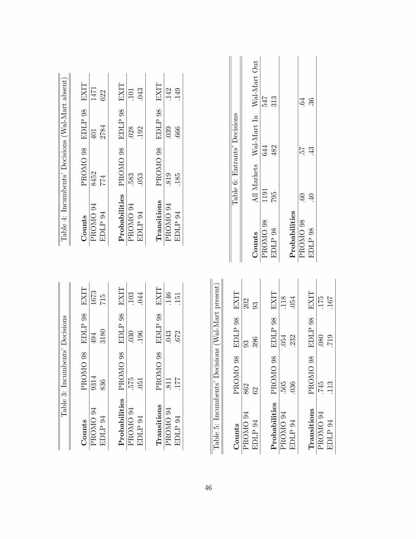
Table3:Incumbents’Decisions

Counts

PROMO98

EDLP98

EXIT

PROMO94

9314

494

1673

EDLP94

836

3180

715

Probabilities

PROMO98

EDLP98

EXIT

PROMO94

.575

.030

.103

EDLP94

.051

.196

.044

Transitions

PROMO98

EDLP98

EXIT

PROMO94

.811

.043

.146

EDLP94

.177

.672

.151

Table4:Incumbents’Decisions(Wal-Martabsent)

Counts

PROMO98

EDLP98

EXIT

PROMO94

8452

401

1471

EDLP94

774

2784

622

Probabilities

PROMO98

EDLP98

EXIT

PROMO94

.583

.028

.101

EDLP94

.053

.192

.043

Transitions

PROMO98

EDLP98

EXIT

PROMO94

.819

.039

.142

EDLP94

.185

.666

.149

Table5:Incumbents’Decisions(Wal-Martpresent)

Counts

PROMO98

EDLP98

EXIT

PROMO94

862

93202

EDLP94

62396

93

Probabilities

PROMO98

EDLP98

EXIT

PROMO94

.505

.054

.118

EDLP94

.036

.232

.054

Transitions

PROMO98

EDLP98

EXIT

PROMO94

.745

.080

.175

EDLP94

.113

.719

.167

Table6:Entrants’Decisions

Counts

AllMarkets

Wal-MartIn

Wal-MartOut

PROMO98

1191

644

547

EDLP98

795

482

313

Probabilities

PROMO98

.60

.57

.64

EDLP98

.40

.43

.36

46

Table7:DescriptivePolicyFunctions

DependentVariable

P(Switch|X)P(Exit|X)P(Enter|X)P(EDLP|X)P(Enter|X)

Wal-Martinlocalmarket

.025

(.016)

.027

(.019)

−.1

41(.041)

.020

(.104)

Wal-MartinMSA

.017

(.006)

.054

(.008)

.035

(.014)

.053

(.039)

EDLP(thisstore)

.136

(.008)

−.0

23(.008)

ShareofEDLP(inlocalmarket)

.010

(.009)

−.0

02(.010)

.005

(.008)

.252

(.034)

.021

(.005)

NumberofRivalStores

.000

8(.0016)

.005

(.002)

−.0

24(.004)

.009

(.007)

.019

(.003)

TotalOwnStores(allmarkets)

−.0

0002

38(.000004)

−.0

0006

5(.00004)

Focus

−.3

42(.035)

−.1

51(.002)

Allregressionsincludeadditionalmarket,storeandchaincontrols

47

Table 8: Distribution of Estimated RevenuesEDLP 5% 50% 95%

Intercept 116.35 273.28 522.26Walmart -48.57 -28.32 -4.21

E(Share of Competitors EDLP) -12.04 0.58 43.22Number of Competitors -12.93 -9.58 -2.49Focus of Chain (EDLP) -12.98 11.11 73.36Total Revenues (Fitted) 185.04 364.05 617.14

PROMO 5% 50% 95%Intercept 115.86 295.48 510.13Walmart -35.13 -20.54 -6.39

E(Share of Competitors EDLP) -15.19 -6.91 3.92Number of Competitors -10.06 -5.86 -1.79

Focus of Chain (PROMO) -12.11 39.22 86.67Total Revenues (Fitted) 255.93 483.77 720.44

48

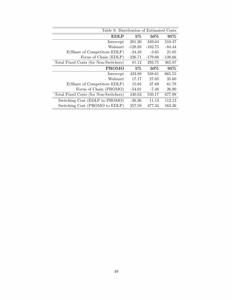
Table 9: Distribution of Estimated Costs

EDLP 5% 50% 95%Intercept 201.20 349.04 510.47Walmart -128.93 -102.75 -84.44

E(Share of Competitors EDLP) -24.33 -3.65 21.05Focus of Chain (EDLP) -226.71 -179.66 -138.66

Total Fixed Costs (for Non-Switchers) 81.12 293.75 465.87

PROMO 5% 50% 95%Intercept 433.89 538.61 665.55Walmart 17.17 27.05 35.60

E(Share of Competitors EDLP) 15.65 37.69 61.78Focus of Chain (PROMO) -54.01 -7.48 26.90

Total Fixed Costs (for Non-Switchers) 440.83 550.17 677.98

Switching Cost (EDLP to PROMO) -30.36 11.13 112.13Switching Cost (PROMO to EDLP) 357.59 477.34 563.36

49

EDLP94

EDLP98 (No Wal-Mart)

PROMO98 (No Wal-Mart)

EDLP98 (Wal-Mart)

PROMO98 (Wal-Mart)

$304K/wk

$302K/wk

$281K/wk

$252K/wk

+$2K/wk(Switch Effect | No Wal-Mart)

+$29K/wk(Switch Effect | Wal-Mart)

PROMO94

EDLP98 (No Wal-Mart)

PROMO98 (No Wal-Mart)

EDLP98 (Wal-Mart)

PROMO98 (Wal-Mart)

$289K/wk

$292K/wk

$284K/wk

$273K/wk

-$11K/wk(Switch Effect | Wal-Mart)

+3K/wk(Switch Effect | No Wal-Mart)

Figure 1: Changes in Revenues by Pricing Format Switch and Wal-Mart Entry

50

Fitted Revenues (PROMO)Frequency

0 200 400 600 800 1000

0500

1000

1500

2000

2500

Fitted Revenues (EDLP)

Frequency

0 200 400 600 800 1000

0500

1000

1500

2000

2500

Change in Revenues (Switch to PROMO)

Frequency

0 50 100 150

050

100

150

Change in Revenues (Switch to EDLP)

Frequency

-150 -100 -50 0

020

4060

80

Figure 2: Counterfactual Revenues

51

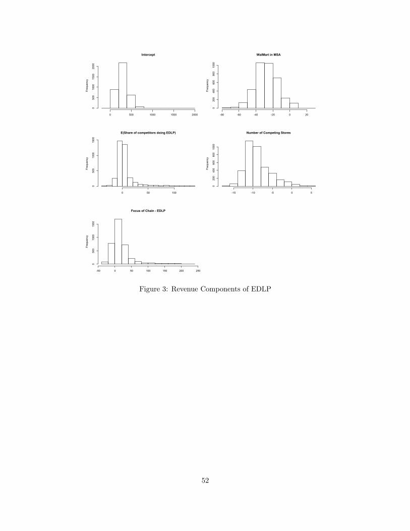
Intercept

Frequency

0 500 1000 1500 2000

0500

1000

1500

2000

WalMart in MSA

Frequency

-80 -60 -40 -20 0 20

0200

400

600

800

1000

E(Share of competitors doing EDLP)

Frequency

0 50 100

0500

1000

1500

Number of Competing Stores

Frequency

-15 -10 -5 0 5

0200

400

600

800

1000

Focus of Chain - EDLP

Frequency

-50 0 50 100 150 200 250

0500

1000

1500

Figure 3: Revenue Components of EDLP

52

Intercept

Frequency

0 500 1000 1500

05001000

2000

3000

WalMart in MSA

Frequency

-50 -40 -30 -20 -10 0

01000

2000

3000

E(Share of competitors doing EDLP)

Frequency

-40 -30 -20 -10 0 10 20 30

01000

2000

3000

4000

Number of Competing Stores

Frequency

-15 -10 -5 0

0500

1000

1500

Focus of Chain - PROMO

Frequency

-200 -150 -100 -50 0 50 100

0500

1500

2500

3500

Figure 4: Revenue Components of PROMO

53

Fixed Costs - EDLPFrequency

0 200 400 600 800 1000

01000

2500

Fixed Costs - PROMO

Frequency

0 200 400 600 800 1000

02000

4000

Figure 5: Estimated Fixed Costs

54

Intercept

Frequency

0 200 400 600 800

01000

3000

WalMart in MSA

Frequency

-200 -150 -100 -50

02000

4000

6000

E(Share of competitors doing EDLP)

Frequency

-100 -50 0 50

02000

4000

6000

Focus (EDLP)

Frequency

-400 -350 -300 -250 -200 -150 -100 -50

02000

4000

6000

Switching Cost

Frequency

200 300 400 500 600

02000

6000

Figure 6: Cost Components of EDLPIntercept

Frequency

300 400 500 600 700 800 900

02000

4000

WalMart in MSA

Frequency

0 20 40 60

02000

5000

E(Share of competitors doing EDLP)

Frequency

0 50 100

02000

4000

Focus (PROMO)

Frequency

-150 -100 -50 0 50 100 150

02000

5000

Switching Cost

Frequency

-50 0 50 100 150 200

02000

4000

Figure 7: Cost Components of PROMO

55

Table A1: Revenue Regression EstimatesPROMO EDLP

Variable Interactions Estimate Std. Error Estimate Std. ErrorIntercept Constant -143.4917 38.4107 2.7606 37.6958

pop 0.0018 0.0003 0.0016 0.0003hhsize 29.4688 13.9660 -27.3737 13.8402

p_black -42.5423 20.5609 -91.7737 26.1777p_urban 38.6491 15.6274 35.6342 15.4588p_hisp 86.2794 32.0506 -105.4643 42.4421h_inc 0.0019 0.0004 0.0023 0.0004size 7.1859 0.1294 7.5947 0.1838

Tstores 0.0099 0.0012 -0.0021 0.0017WalMart Constant 3.4924 18.9370 40.0459 26.8277

pop -0.0001 0.0001 0.0000 0.0002hhsize 0.1696 7.0774 -9.5970 10.6311

p_black -3.0332 12.1695 2.5743 16.0800p_urban -8.0267 8.3187 -32.4061 12.0374p_hisp -36.8025 14.2069 39.5778 29.9141h_inc -0.0001 0.0002 -0.0007 0.0004

E(Comp EDLP) Constant 45.4532 23.3660 -11.8019 35.9686pop 0.0000 0.0002 -0.0005 0.0003

hhsize -16.0171 8.4788 6.4146 13.4419p_black 18.2148 12.6664 4.5995 19.9579p_urban -15.2756 10.2790 7.1724 11.4828p_hisp 21.1111 20.4637 129.1107 32.3871h_inc 0.0002 0.0002 -0.0001 0.0005

Focus PROMO/EDLP Constant 185.2156 42.4260 -120.8199 45.5139pop -0.0006 0.0003 -0.0007 0.0004

hhsize -71.4293 15.7550 53.6338 16.7937p_black 45.4121 23.8604 12.8066 26.6348p_urban -9.0338 15.8865 27.3170 17.3471p_hisp -43.4603 34.4132 120.7215 38.8835h_inc 0.0006 0.0004 -0.0007 0.0006

Number of Competing Constant 3.4682 4.4740 1.9628 6.2802Stores pop -0.0001 0.0000 0.0000 0.0000

hhsize -0.9573 1.3945 -3.8233 2.2772p_black -2.4410 2.2300 15.6963 3.7920p_urban -1.5155 1.9349 -2.4647 2.5457p_hisp 8.0419 3.5968 17.2897 8.5114h_inc -0.0001 0.0000 0.0000 0.0001

56

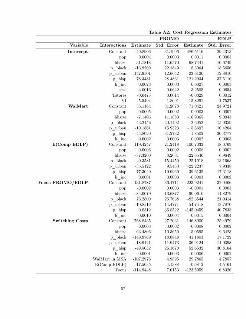
Table A2: Cost Regression EstimatesPROMO EDLP

Variable Interactions Estimate Std. Error Estimate Std. ErrorIntercept Constant -40.8906 31.1996 486.5116 29.4313

pop 0.0004 0.0003 0.0011 0.0003hhsize 31.1818 11.6570 -68.7441 10.6749

p_black -16.9209 22.1849 18.3064 18.5656p_urban 147.9501 12.6642 23.6120 12.8810p_hisp 78.3481 28.4861 121.2934 37.5116h_inc 0.0023 0.0003 0.0027 0.0003size 4.0016 0.0642 3.2505 0.0654

Tstores -0.0475 0.0014 -0.0329 0.0012VI 5.5494 1.8091 15.8291 1.7537

WalMart Constant 36.1164 31.2078 71.0421 24.9721pop -0.0005 0.0002 0.0003 0.0002

hhsize -7.1406 11.1883 -16.9365 9.0943p_black 43.2456 20.1492 2.6052 15.9359p_urban -10.1861 15.9323 -15.6697 10.4204p_hisp -44.8020 31.2732 1.8502 20.3777h_inc 0.0002 0.0003 0.0002 0.0003

E(Comp EDLP) Constant 119.4247 21.2418 100.7033 18.6769pop 0.0006 0.0002 0.0008 0.0002

hhsize -37.3200 8.2631 -22.6546 6.9649p_black -0.3581 15.4459 25.1018 13.1668p_urban -35.5122 9.5463 -22.2237 7.9338p_hisp 77.3049 19.9969 39.6135 17.3118h_inc 0.0001 0.0003 -0.0003 0.0002

Focus PROMO/EDLP Constant 131.8787 36.4711 -223.9241 32.9406pop -0.0002 0.0003 -0.0001 0.0003

hhsize -84.0079 13.6877 90.0610 11.8279p_black 76.2809 26.7638 -82.3544 21.9314p_urban -10.8516 14.4771 54.7418 13.7870p_hisp 0.8312 36.8522 -145.0459 40.7833h_inc 0.0010 0.0004 -0.0015 0.0004

Switching Costs Constant 768.8435 27.2031 146.8000 25.4979pop 0.0003 0.0002 -0.0008 0.0002

hhsize -63.4806 10.3650 -5.0595 9.6423p_black -149.9769 18.6848 41.1803 17.1722p_urban -18.9121 11.9473 -36.9124 11.0398p_hisp -49.5052 26.1670 52.6532 30.8164h_inc -0.0001 0.0003 0.0006 0.0002

WalMart in MSA -107.2976 4.9895 29.7865 4.7857E(Comp EDLP) -17.5035 4.1388 -0.6812 4.5161

Focus -114.9448 7.0153 -123.5959 6.8326

57