REPORTS - AVACS: Start · A Temporal Dynamic Logic for Verifying Hybrid System Invariants by...

AVACS – Automatic Verification and Analysis of

Complex Systems

REPORTSof SFB/TR 14 AVACS

Editors: Board of SFB/TR 14 AVACS

A Temporal Dynamic Logic for

Verifying Hybrid System Invariants

by

Andre Platzer

AVACS Technical Report No. 12February 2007

ISSN: 1860-9821

Publisher: Sonderforschungsbereich/Transregio 14 AVACS(Automatic Verification and Analysis of Complex Systems)

Editors: Bernd Becker, Werner Damm, Martin Franzle, Ernst-Rudiger Olderog,Andreas Podelski, Reinhard Wilhelm

ATRs (AVACS Technical Reports) are freely downloadable from www.avacs.org

Copyright c© February 2007 by the author(s)

Author(s) contact: Andree Platzer ([email protected]).

A Temporal Dynamic Logic for

Verifying Hybrid System Invariants⋆

Andre Platzer

University of Oldenburg, Department of Computing Science, GermanyCarnegie Mellon University, Computer Science Department, Pittsburgh, PA

[email protected]

Abstract. We combine first-order dynamic logic for reasoning aboutpossible behaviour of hybrid systems with temporal logic for reasoningabout the temporal behaviour during their operation. Our logic sup-ports verification of hybrid programs with first-order definable flows andprovides a uniform treatment of discrete and continuous evolution. Forour combined logic, we generalise the semantics of dynamic modalitiesto refer to hybrid traces instead of final states. Further, we prove thatthis gives a conservative extension of dynamic logic. On this basis, weprovide a modular verification calculus that reduces correctness of tem-poral behaviour of hybrid systems to non-temporal reasoning. Using thiscalculus, we analyse safety invariants in a train control system and sym-bolically synthesise parametric safety constraints.

Keywords: dynamic logic, temporal logic, sequent calculus, logic forhybrid systems, deductive verification of embedded systems

1 Introduction

Correctness of real-time and hybrid systems depends on a safe operation through-out all states of all possible trajectories, and the behaviour at intermediate statesis highly relevant [1, 7, 9, 12, 14, 23].

Temporal logics (TL) use temporal operators to talk about intermediatestates [1, 10, 11, 24]. They have been used successfully in model checking [1, 6,14, 15, 18] of finite-state system abstractions. Continuous state spaces of hybridsystems, however, often do not admit equivalent finite-state abstractions [14,18].Instead of model checking, TL can also be used deductively to prove validity offormulas in calculi [8, 9]. Valid TL formulas, however, only express very genericfacts that are true for all systems, regardless of their actual behaviour. Hence,the behaviour of a specific system first needs to be axiomatised declarativelyto obtain meaningful results. Then, however, the correspondence between actualsystem operations and a declarative temporal representation may be questioned.

⋆ This research was supported by a fellowship of the German Academic ExchangeService (DAAD). It was also sponsored by the German Research Council (DFG)as part of the Transregional Collaborative Research Center “Automatic Verificationand Analysis of Complex Systems” (SFB/TR 14 AVACS, see www.avacs.org). Ashorter version [21] of this report appeared at LFCS 2007.

2 Andre Platzer

Dynamic logic (DL) [13] is a successful approach for deductively verifying(infinite-state) systems [2, 3, 13, 16]. Like model checking, DL can analyse thebehaviour of actual system models, which are specified operationally. Yet, op-erational models are internalised within DL-formulas, and DL is closed underlogical operators. Thus, DL can refer to multiple systems and analyse their rela-tionship. This can be important for verifying larger systems compositionally orfor investigating refinement relations, see [22]. Further, Davoren and Nerode [9]argue that, unlike model checking, deductive methods support formulas with freeparameters. However, DL only considers the behaviour at final states, which isinsufficient for verifying safety invariants that have to hold all the time.

We close this gap of expressivity by combining first-order dynamic logic [13]with temporal logic [10,11,24]. Moreover, we generalise both operational systemmodels and semantics to hybrid systems [14]. In this paper, we introduce atemporal dynamic logic dTL, which provides modalities for quantifying overtraces of hybrid systems. We equip it with temporal operators to state what istrue all along a trace or at some point during a trace. As in our non-temporaldynamic logic dL [19, 20, 22], we use hybrid programs as an operational modelfor hybrid systems. They admit a uniform treatment of interacting discrete andcontinuous evolution in logic.

As a semantical foundation for combined temporal dynamic formulas, weintroduce a hybrid trace semantics for dTL. We prove that dTL is a conservativeextension of dL: for non-temporal specifications, trace semantics is equivalent tothe non-temporal final state semantics of [19, 22].

As a means for verification, we introduce a sequent calculus for dTL thatsuccessively reduces temporal statements about traces of hybrid programs tonon-temporal formulas. In this way, we make the intuition formally precise thatsafety invariants can be checked by augmenting proofs with appropriate asser-tions about intermediate states. Like in [22], our calculus supports compositionalreasoning. It structurally decomposes correctness statements about hybrid pro-grams into corresponding statements about its parts by symbolic transformation.

Our approach combines the advantages of DL in reasoning about the be-haviour of (multiple and parametric) operational system models with those ofTL to verify temporal statements about traces. On the downside, we show thatour logic is incomplete. Yet, reachability in hybrid systems is already unde-cidable [14]. We argue that, despite this theoretical obstacle, dTL can verifypractical systems and demonstrate this by studying safety invariants in traincontrol [7, 12].

The first contribution of this paper is the logic dTL, which provides a coherentfoundation for reasoning about the temporal behaviour of operational models ofhybrid systems with symbolic parameters. The main contribution is our calculusfor deductively verifying temporal statements about hybrid systems.

Hybrid Systems. The behaviour of safety-critical systems typically depends onboth the state of a discrete controller and continuous physical quantities. Hybridsystems are mathematical models for dynamic systems with interacting discrete

A Temporal Dynamic Logic for Verifying Hybrid System Invariants 3

and continuous behaviour [9,14]. Their behaviour combines continuous evolution(called flow) characterised by differential equations and discrete jumps.

Dynamic Logic. The principle of dynamic logic is to combine system operationsand correctness statements about system states within a single specificationlanguage (see [13] for a general introduction in the discrete case). By permittingsystem operations α as actions of modalities, dynamic logic provides formulasof the form [α]φ and 〈α〉φ, where [α]φ expresses that all terminating runs ofsystem α lead to final states in which condition φ holds. Likewise, 〈α〉φ expressesthat it is possible for α to execute and result in a final state satisfying φ. IndTL, hybrid programs [19, 20, 22] play the role of α. In this paper, we modifythe semantics of [α] to refer to all traces of α rather than only all final statesreachable with α (similarly for 〈α〉). For instance, the formula [α]�φ expressesthat φ is true at each state during all traces of the hybrid system α. With this,dTL can also be used to verify temporal statements about the behaviour of αat intermediate states during system runs.

Related Work. Based on [25], Beckert and Schlager [4] added separate tracemodalities to dynamic logic and presented a relatively complete calculus. Theirapproach only handles discrete state spaces. In contrast, dTL works for hybridprograms with continuous state spaces. There, a particular challenge is thatinvariants may change their truth-value during a single continuous evolution.

Mysore et al. [18] analysed model checking of TCTL [1] properties for semi-algebraic hybrid systems and proved undecidability. Our logic internalises oper-ational models and supports multiple parametric systems.

Zhou et al. [26] presented a duration calculus extended by mathematicalexpressions with derivatives of state variables. Their calculus is unwieldy as ituses a multitude of rules and requires external mathematical reasoning aboutderivatives and continuity.

Davoren and Nerode [9] extended the propositional modal µ-calculus with asemantics in hybrid systems and examine topological aspects. In [8], Davoren etal. gave a semantics in general flow systems for a generalisation of CTL

∗ [11].In both cases, the authors of [9] and [8] provided Hilbert-style calculi to proveformulas that are valid for all systems simultaneously using abstract actions.

The strength of our logic primarily is that it is a first-order dynamic logic: ithandles actual hybrid programs like x := x+ 1; x = 2y rather than only abstractactions of unknown effect. Our calculus directly supports verification of hybridprograms with first-order definable flows; first-order approximations of moregeneral flows can be used according to [23]. First-order DL is more expressiveand calculi are deductively stronger than other approaches [4, 17].

Structure of this Paper. After introducing syntax and semantics of the temporaldynamic logic dTL in Sect. 2, we introduce a sequent calculus for verifyingtemporal dTL specifications of hybrid systems in Sect. 4 and prove soundness. InSect. 5, we prove safety invariants of the train control system presented in Sect. 3.

4 Andre Platzer

Alternating path and trace quantifiers for liveness verification are discussed inSect. 6. Finally, we draw conclusions and discuss future work in Sect. 7.

2 Temporal Dynamic Logic for Hybrid Systems

2.1 Overview: The Basic Concepts of dTL

The temporal dynamic logic dTL extends dynamic logic [13] with three conceptsfor verifying temporal specifications of hybrid systems:

Hybrid programs. The behaviour of hybrid systems can be described by hybridprograms [19,20,22], which generalise real-time programs [15] to hybrid change.The distinguishing feature of hybrid programs in this context is that they provideuniform discrete jumps and continuous evolutions along differential equations.While hybrid automata [14] can be embedded, program structures are moreamenable to compositional symbolic processing by calculus rules [19].

Modal operators. Modalities of dynamic logic express statements about all pos-sible behaviour ([α]π) of a system α, or about the existence of a trace (〈α〉π),satisfying condition π. As in [19, 20, 22], the system α is described as a hybridprogram. Yet, unlike in standard dynamic logic [13], π is a trace formula in dTL,and π is allowed to refer to all states that occur during a trace using temporaloperators.

Temporal operators. For dTL, the temporal trace formula �φ expresses that theformula φ holds all along a trace selected by [α] or 〈α〉. For instance, the stateformula 〈α〉�φ says that the state formula φ holds at every state along at leastone trace of α. Dually, the trace formula ♦φ expresses that φ holds at some pointduring such a trace. It can occur in a state formula 〈α〉♦φ to express that thereis such a state in some trace of α, or as [α]♦φ to say that, along each trace,there is a state satisfying φ. In this paper, the primary focus of attention is onhomogeneous combinations of path and trace quantifiers like [α]�φ or 〈α〉♦φ.

2.2 Syntax of dTL

State and Trace Formulas. The formulas of dTL are built over a non-emptyset V of real-valued variables and a fixed signature Σ of function and predicatesymbols. For simplicity, Σ is assumed to contain exclusively the usual functionand predicate symbols for real arithmetic, such as 0, 1,+, ·,=,≤, <,≥, >.

The set Trm(V ) of terms is defined as in classical first-order logic. The for-mulas of dTL are defined similar to first-order dynamic logic [13]. However, themodalities [α] and 〈α〉 accept trace formulas that refer to the temporal behaviourof all states along a trace. Inspired by CTL and CTL

∗ [10, 11], we distinguishbetween state formulas, that are true or false in states, and trace formulas, thatare true or false for system traces. The sets Fml(V ) of state formulas, FmlT (V )of trace formulas, and HP(V ) of hybrid programs with variables in V are simul-taneously inductively defined in Definition 1 and 2, respectively.


Definition 1 (Formulas). The set Fml(V ) of (state) formulas is simultane-ously inductively defined as the smallest set such that:

1. If p ∈ Σ is a predicate, θ1, . . . , θn ∈ Trm(V ), then p(θ1, . . . , θn) ∈ Fml(V ).2. If φ, ψ ∈ Fml(V ), then ¬φ, (φ ∧ ψ), (φ ∨ ψ), (φ→ ψ) ∈ Fml(V ).3. If φ ∈ Fml(V ) and x ∈ V , then ∀xφ, ∃xφ ∈ Fml(V ).4. If π ∈ FmlT (V ) and α ∈ HP(V ), then [α]π, 〈α〉π ∈ Fml(V ).

The set FmlT (V ) of trace formulas is the smallest set with:

1. If φ ∈ Fml(V ), then φ ∈ FmlT (V ).2. If φ ∈ Fml(V ), then �φ,♦φ ∈ FmlT (V ).

Formulas without � and ♦, i.e., without case 2 of the trace formulas, are callednon-temporal dL formulas [19, 22]. Unlike in CTL, state formulas are true on atrace (case 1) if they hold for the last state of a trace, not for the first. Thus, [α]φexpresses that φ is true at the end of each trace of α. In contrast, [α]�φ expressesthat φ is true all along all states of every trace of α. This combination gives asmooth embedding of non-temporal dL into dTL and makes it possible to definea compositional calculus. Like CTL, dTL allows nesting with a branching timesemantics [10], e.g., [α]�(x ≥ 2 → 〈γ〉♦x ≤ 0).

Hybrid Programs. The hybrid programs [19, 20, 22] occurring in dynamicmodalities of dTL are built from elementary discrete jumps and continuous evo-lutions using a regular control structure [13].

Definition 2 (Hybrid programs). The set HP(V ) of hybrid programs isinductively defined as the smallest set such that:

1. If x ∈ V and θ ∈ Trm(V ), then (x := θ) ∈ HP(V ).2. If x ∈ V and θ ∈ Trm(V ), then (x = θ) ∈ HP(V ).3. If χ ∈ Fml(V ) is quantifier-free and first-order, then (?χ) ∈ HP(V ).4. If α, γ ∈ HP(V ) then (α ∪ γ) ∈ HP(V ).5. If α, γ ∈ HP(V ) then (α; γ) ∈ HP(V ).6. If α ∈ HP(V ) then (α∗) ∈ HP(V ).

The effect of x := θ is an instantaneous discrete jump in state space or a modeswitch. That of x = θ is an ongoing continuous evolution regulated by thedifferential equation with time-derivative x of x and term θ (accordingly forsystems of differential equations).

Test actions ?χ are used to define conditions. Their semantics is that ofa no-op if χ is true in the current state, and that of a dead end operatoraborting any further evolution, otherwise. The sequential composition α; γ, non-deterministic choice α∪γ, and non-deterministic repetition α∗ of system actionsare as usual [13]. They can be combined with ?χ to form other control struc-tures [13].

In dTL, there is no need to distinguish between discrete and continuous vari-ables or between system parameters and state variables, as they share the same

6 Andre Platzer

uniform semantics. For pragmatic reasons, an informal distinction can neverthe-less improve readability. For instance, ∃x [x = −x]x ≤ 5 expresses that there is achoice of the initial value for x (which could be a parameter) such that after allevolutions along x = −x, the outcome of the state variable x will be at most 5.

2.3 Trace Semantics of dTL

In standard dynamic logic [13] and dL [19,22], modalities only refer to the finalstates of system runs and the semantics is a reachability relation on states:State ω is reachable from state ν using α if there is a run of α which terminatesin ω when started in ν. For dTL, however, formulas can refer to intermediatestates of runs as well. Thus, the semantics of a hybrid system α is the set of itspossible traces, i.e., successions of states that occur during the evolution of α.

States contain values of system variables during a hybrid evolution. A stateis a map ν : V → R; the set of all states is denoted by Sta(V ). In addition, wedistinguish a state Λ to denote the failure of a system run when it is aborted dueto a test ?χ that yields false . In particular, Λ can only occur at the end of anaborted system run and marks that there is no further extension.

Hybrid systems evolve along piecewise continuous traces in multi-dimensionalspace as time passes. Continuous phases are governed by differential equations,whereas discontinuities are caused by discrete jumps in state space. Unlike indiscrete cases [4,25], traces are not just sequences of states, since hybrid systemspass through uncountably many states even in bounded time. Beyond that, con-tinuous changes are more involved than in pure real-time [1, 15], because allvariables can evolve along different differential equations. Generalising the real-time traces of [15], the following definition captures hybrid behaviour by splittingthe uncountable succession of states into periods σi that are regulated by thesame control law. For discrete jumps, some periods are point flows of duration 0.

Definition 3 (Hybrid Trace). A trace is a (non-empty) finite or infinite se-quence σ = (σ0, σ1, σ2, . . . ) of functions σi : [0, ri] → Sta(V ) with respective du-rations ri ∈ R (for i ∈ N). A position of σ is a pair (i, ζ) with i ∈ N and ζ inthe interval [0, ri]; the state of σ at (i, ζ) is σi(ζ). Positions of σ are orderedlexicographically by (i, ζ) ≺ (j, ξ) iff either i < j, or i = j and ζ < ξ. Further,for a state ν ∈ Sta(V ), ν : 0 7→ ν is the point flow at ν with duration 0. A traceterminates if it is a finite sequence (σ0, σ1, . . . , σn) and σn(rn) 6= Λ. In that case,the last state lastσ is denoted as σn(rn). The first state firstσ is σ0(0).

Unlike in [1,15], the definition of traces also admits finite traces of bounded du-ration, which is necessary for compositionality of traces in α; γ. The semanticsof hybrid programs α as the set τ(α) of its possible traces depends on valua-tions val(ν, ·) of formulas and terms at intermediate states ν. The valuation ofterms [13], and interpretations of function and predicate symbols are as usualfor real arithmetic. The valuation of formulas will be defined in Definition 5. Weuse ν[x 7→ d] to denote the modification that agrees with state ν on all variablesexcept for the symbol x, which is changed to d ∈ R.


Definition 4 (Trace semantics of hybrid programs). The trace semantics,τ(α), of a hybrid program α, is the set of all its possible hybrid traces and isdefined as follows:

1. τ(x := θ) = {(ν, ω) : ω = ν[x 7→ val(ν, θ)] for ν ∈ Sta(V )}2. τ(x = θ) = {(f) : 0 ≤ r ∈ R and f : [0, r] → Sta(V ) is such that the func-

tion val(f(ζ), x) is continuous in ζ on [0, r] and has a derivative of valueval(f(ζ), θ) at each ζ ∈ (0, r). Variables without a differential equation donot change}

3. τ(?χ) = {(ν) : val(ν, χ) = true} ∪ {(ν, Λ) : val(ν, χ) = false}4. τ(α ∪ γ) = τ(α) ∪ τ(γ)5. τ(α; γ) = {σ ◦ ς : σ ∈ τ(α) , ς ∈ τ(γ) when σ ◦ ς is defined}; the composition

of σ = (σ0, σ1, σ2, . . . ) and ς = (ς0, ς1, ς2, . . . ) is

σ ◦ ς =

(σ0, . . . , σn, ς0, ς1, . . . ) if σ terminates at σn and lastσ = first ς

σ if σ does not terminate

not defined otherwise

6. τ(α∗) =⋃

n∈Nτ(αn), where αn+1 = (αn;α) for n ≥ 1, and α0 = (?true).

Time passes differently during discrete and continuous change. During contin-uous evolution, the discrete step index i of positions (i, ζ) remains constant,whereas the continuous duration ζ remains 0 during discrete point flows. Thispermits multiple discrete state changes to happen at the same (super-dense)continuous time, unlike in [1].

Definition 5 (Valuation of formulas). The valuation of state and trace for-mulas is defined respectively. For state formulas, the valuation val(ν, ·) withrespect to state ν is defined as follows:

1. val(ν, p(θ1, . . . , θn)) = pℓ(

val(ν, θ1), . . . , val(ν, θn))

, where pℓ is the relationassociated to p.

2. val(ν, φ ∧ ψ) is defined as usual, the same holds for ¬,∨,→.3. val(ν, ∀xφ) = true :⇐⇒ val(ν[x 7→ d], φ) = true for all d ∈ R

4. val(ν, ∃xφ) = true :⇐⇒ val(ν[x 7→ d], φ) = true for some d ∈ R

5. val(ν, [α]π) = true :⇐⇒ for each trace σ ∈ τ(α) that starts in firstσ = ν, ifval(σ, π) is defined, then val(σ, π) = true.

6. val(ν, 〈α〉π) = true :⇐⇒ there is a trace σ ∈ τ(α) starting in firstσ = ν,such that val(σ, π) = true.

For trace formulas, the valuation val(σ, ·) with respect to trace σ is:

1. If φ is a state formula, then val(σ, φ) = val(lastσ, φ) if σ terminates,whereas val(σ, φ) is not defined if σ does not terminate.

2. val(σ,�φ) = true :⇐⇒ val(σi(ζ), φ) = true for all positions (i, ζ) of σwith σi(ζ) 6= Λ.

3. val(σ,♦φ) = true :⇐⇒ val(σi(ζ), φ) = true for some position (i, ζ) of σwith σi(ζ) 6= Λ.

As usual, a (state) formula is valid if it is true in all states.

8 Andre Platzer

2.4 Conservative Temporal Extension

The following result shows that the extension of dTL by temporal operators doesnot change the meaning of non-temporal dL formulas. The trace semantics givenin Definition 5 is equivalent to the final state reachability relation semantics [19,22] for the sublogic dL of dTL. A proof for this can be found in appendix B.

Proposition 1. The logic dTL is a conservative extension of non-temporal dL,i.e., the set of valid dL-formulas is the same with respect to transition reach-ability semantics of dL [19, 22] as with respect to the trace semantics of dTL(Definition 5).

3 Safety Invariants in Train Control

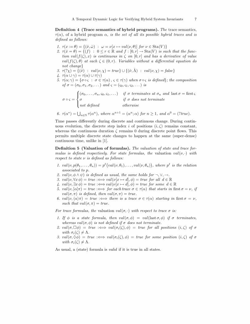
In the European Train Control System (ETCS) [12], trains are coordinated bydecentralised Radio Block Centres (RBC), which grant or deny movement au-thorities (MA) to the individual trains by wireless communication. In emergen-cies, trains always have to stop within the MA issued by the RBC, see Fig. 1.Following the reasoning pattern for traffic agents in [7], each train negotiateswith the RBC to extend its MA when approaching the end, say m, of its cur-rent MA. Since wireless communication takes time, this negotiation is initiatedin due time before reaching m. During negotiation, trains are assumed to keeptheir desired speed as in [7]. Before entering negotiation at some point ST, thetrain still has sufficient distance to MA (it is in far mode) and can regulate itsspeed freely within the track limits.

Depending on weather conditions, slope of track etc., the local train motioncontrol determines a safety envelope s around the train, within which it con-siders driving safe, and adjusts its acceleration a in accordance with s (calledcorrection [7]). In particular, depending on the maximum RBC response time,this determines the latest point, SB, on the track where a response from theRBC must have arrived to guarantee safe driving.

RBC

MAST SBnegot corrfar

Fig. 1. ETCS train coordination by movement authorities

As a model for train movements, we use the ideal-world model adaptedfrom [7]. It does not model friction, slopes, or mass of train but is perfectlysuitable for analysing the cooperation level of train control [7]. The local safety


properties that where used when verifying the cooperation protocol can then beshown for more detailed models of individual components.

For a safe operation of multiple traffic agents, it is crucial that the MA isrespected at every point in time during this protocol, not only at its end. Hence,we need to consider temporal safety invariants. For instance, when the train hasentered the negotiation phase at its current position z, dTL can analyse thefollowing safety invariant of a part of the train controller:

ψ → [negot; corr; z = v, v = a]�(ℓ ≤ L→ z < m) (1)

where negot ≡ z = v, ℓ = 1

corr ≡ (?m− z < s; a := −b) ∪ (?m− z ≥ s; a := . . . ) .

It expresses that—under a sanity condition ψ for parameters—a train will alwaysremain within its MA m, as long as the accumulated RBC negotiation latency ℓis at most L. We refer to [12] for details on what contributes to ℓ. Like in [7], wemodel the train to first negotiate while keeping a constant speed (z = v) in negot.Thereafter, in corr , the train corrects its acceleration or brakes with force b (asa failsafe recovery manoeuvre) on the basis of the remaining distance (m − z).Finally, the train continues moving according to the system (z = v, v = a) or,equivalently, z = a. Instead of manually choosing specific values for the freeparameters of (1) as in [7,12], we will use the techniques developed in this paperto automatically synthesise constraints on the relationship of parameters thatare required for a safe operation of cooperative train control.

4 A Verification Calculus for Safety Invariants

In this section, we introduce a sequent calculus for verifying temporal specifica-tions of hybrid systems in dTL. With the basic idea being to perform a sym-bolic decomposition, hybrid programs are successively transformed into simplerlogical formulas describing their effects. There, statements about the temporalbehaviour of a hybrid program are successively reduced to corresponding non-temporal statements about the intermediate states.

For propositional logic, standard rules P1–P9 are listed in Fig. 2. The rule P10is a shortcut to handle quantifiers of first-order real arithmetic, which is decid-able. We use P10 as a modular interface to arithmetic and refer to [19] for agoal-oriented integration of arithmetic, which combines with dTL. Rules D1–D8work similar to those in [3,13]. For handling discrete change, D8 inductively usessubstitutions. D9–D10 handle continuous evolutions given a first-order definableflow yx. In particular, in conjunction with P10, they fully encapsulate handlingof differential equations within hybrid systems.

Rules T1–T10 successively transform temporal specifications of hybrid pro-grams into non-temporal dL formulas. The idea underlying this transformationis to decompose hybrid programs and recursively augment intermediate statetransitions with appropriate specifications. D1–D2 are identical for dTL and dLspecifications, hence they apply for all trace formulas π and not just for stateformulas. Rules for handling [α]♦φ and 〈α〉�φ are discussed in Sect. 6.

10 Andre Platzer

4.1 Rules of the Calculus

A sequent is of the form Γ ⊢ ∆, where Γ and ∆ are finite sets of formulas. Itssemantics is that of the formula

∧

φ∈Γ φ →∨

ψ∈∆ ψ and will be treated as anabbreviation. In the following, an update U is a list of discrete assignments ofthe form x := θ (see [3] for advanced update techniques, which can be combinedwith our calculus).

Definition 6 (Provability, derivability). A formula ψ is provable from aset Φ of formulas, denoted by Φ ⊢dTL ψ iff there is a finite set Φ0 ⊆ Φ for whichthe sequent Φ0 ⊢ ψ is derivable. In turn, a sequent of the form Γ, 〈U〉Φ ⊢ 〈U〉Ψ,∆(for some update U , including the empty update, and finite sets Γ,∆ of contextformulas) is derivable iff there is an instance

Φ1 ⊢ Ψ1 . . . Φn ⊢ Ψn

Φ ⊢ Ψ

of a rule schema of the dTL calculus in Fig. 2 such that

Γ, 〈U〉Φi ⊢ 〈U〉Ψi, ∆

is derivable for each 1 ≤ i ≤ n. Moreover, the symmetric schemata Di and T i

can be applied on either side of the sequent (in context Γ,∆ and update 〈U〉).The schematic modality 〈[·]〉 can be instantiated with both [·] and 〈·〉 in all ruleschemata. The same modality instance has to be chosen within a single schemainstantiation, though.

As usual in sequent calculus—although the direction of entailment is from pre-misses (above rule bar) to conclusion (below)—the order of reasoning is goal-directed : Rules are applied starting from the desired conclusion at the bottom(goal) to the premisses (sub-goals).

Rule T1 decomposes invariants of α; γ into an invariant of α and an invariantof γ that holds when γ is started in any final state of α. T3 expresses that invari-ants of assignments need to hold before and after the discrete change (similarlyfor T2, except that tests do not lead to a state change). T4 can directly reduceinvariants of continuous evolutions to non-temporal formulas as restrictions ofsolutions of differential equations are themselves solutions of different duration.T5 relies on T1 and is simpler than D7, because the other rules will inductivelyproduce a premiss that φ holds in the current state. The dual rules T6–T10work similarly. The usual induction schemes [13, 17] can be added to the dTLcalculus. Inductive invariant properties can be handled by augmenting inductionrules with an additional branch that takes care of the temporal properties.

4.2 Soundness and Incompleteness

The following result shows that verification with the dTL calculus always pro-duces correct results about safety of hybrid systems, i.e., the dTL calculus issound.


(P1)⊢ φ

¬φ ⊢

(P2)φ ⊢

⊢ ¬φ

(P3)φ ⊢ ψ

⊢ φ→ ψ

(P4)φ, ψ ⊢

φ ∧ ψ ⊢

(P5)⊢ φ ⊢ ψ

⊢ φ ∧ ψ

(P6)⊢ φ ψ ⊢

φ→ ψ ⊢

(P7)φ ⊢ ψ ⊢

φ ∨ ψ ⊢

(P8)⊢ φ, ψ

⊢ φ ∨ ψ

(P9)φ ⊢ φ

(P10)F0 ⊢ G0

F ⊢ G

(D1)〈α〉π ∨ 〈γ〉π

〈α ∪ γ〉π

(D2)[α]π ∧ [γ]π

[α ∪ γ]π

(D3)〈[α]〉〈[γ]〉φ

〈[α; γ]〉φ

(D4)χ ∧ φ

〈?χ〉φ

(D5)χ→ φ

[?χ]φ

(D6)φ ∨ 〈α;α∗〉φ

〈α∗〉φ

(D7)φ ∧ [α;α∗]φ

[α∗]φ

(D8)F θ

x

〈[x := θ]〉F

(D9)∃t≥0 〈x := yx(t)〉φ

〈x = θ〉φ

(D10)∀t≥0 [x := yx(t)]φ

[x = θ]φ

(T1)[α]�φ ∧ [α][γ]�φ

[α; γ]�φ

(T2)φ

[?χ]�φ

(T3)φ ∧ [x := θ]φ

[x := θ]�φ

(T4)[x = θ]φ

[x = θ]�φ

(T5)[α;α∗]�φ

[α∗]�φ

(T6)〈α〉♦φ ∨ 〈α〉〈γ〉♦φ

〈α; γ〉♦φ

(T7)φ

〈?χ〉♦φ

(T8)φ ∨ 〈x := θ〉φ

〈x := θ〉♦φ

(T9)〈x = θ〉φ

〈x = θ〉♦φ

(T10)〈α;α∗〉♦φ

〈α∗〉♦φ

In these rules, φ and ψ are (state) formulas, whereas π is a trace formula. Unlike φand ψ, the trace formula π may thus begin with � or ♦. In D8, F is a first-orderformula and the substitution of F θ

x , which replaces x by θ in F , does not introducenew bindings. In D9–D10, t is a fresh variable and yv the solution of the initial valueproblem (x = θ, x(0) = v). In P10, Cl∀ (F0 → G0) → Cl∀ (F → G) is an instance of afirst-order tautology of real arithmetic and Cl∀ the universal closure.

Fig. 2. Rule schemata of the temporal dynamic dTL verification calculus.

12 Andre Platzer

Theorem 1 (Soundness). The dTL calculus is sound, i.e., derivable (state)formulas are valid. (See appendix A.1 for a proof.)

Theorem 2 (Incompleteness). Fragments of dTL are inherently incomplete,i.e. cannot have a complete calculus. (See appendix A.2 for a proof.)

5 Verification of Train Control Safety Invariants

Continuing the ETCS study from Sect. 3, we consider a slightly simplified versionof equation (1) that gives a more concise proof. By a safe abstraction (provablein dTL), we simplify corr to permit braking even when m− z ≥ s, since brakingremains safe with respect to z < m. We use the following abbreviations inaddition to (1):

ψ ≡ z < m ∧ v > 0 ∧ ℓ = 0 ∧ L ≥ 0

φ ≡ ℓ ≤ L→ z < m

corr ≡ a := −b ∪ (?m− z ≥ s; a := . . . ) .

Within the following proof, 〈[]〉 brackets are used instead of modalities to visuallyidentify the update prefix (Definition 6). To give shorter formulas, we generaliseupdate application D8 to work within quantifiers according to [3]. The dTL proofof the safety invariant in (1) splits into two cases as follows:

. . .

ψ ⊢ [negot]�φ. . .

ψ ⊢ [negot][corr; z = v, v = a]�φT1 ψ ⊢ [negot; corr; z = v, v = a]�φP3 ⊢ ψ → [negot; corr; z = v, v = a]�φ

There, the left branch proves that φ holds while negotiating and is as follows:

ψ ⊢ Lv + z < mP10ψ ⊢ ∀l≥0 (l ≤ L→ lv + z < m)D8 ψ ⊢ ∀l≥0 〈[z := lv + z, ℓ := l]〉φD10ψ ⊢ [negot]φT4 ψ ⊢ [negot]�φ

The right branch shows that φ continues to hold after negotiation has completedwhen continuing with an adjusted acceleration a:

ψ, ℓ≥0 ⊢ v2 < 2b(m− Lv − z) ∧ Lv + z < mP10 ψ, ℓ≥0 ⊢ 〈[z := ℓv+z, a := -b]〉∀t≥0 (ℓ≤L→ a

2 t2+vt+z<m)

D8 ψ, ℓ≥0 ⊢ 〈[z := ℓv+z, a := -b]〉∀t≥0 〈[z := a2 t

2+vt+z]〉φ)T4,D10ψ, ℓ≥0 ⊢ 〈[z := ℓv+z, a := -b]〉[z = v, v = a]�φ ⊲

D2 ψ, ℓ≥0 ⊢ 〈[z := ℓv+z]〉[corr][z = v, v = a]�φ ⊲T1 ψ, ℓ≥0 ⊢ 〈[z := ℓv+z]〉[corr; z = v, v = a]�φP3 ψ ⊢ ℓ≥0 → 〈[z := ℓv+z]〉[corr; z = v, v = a]�φP10 ψ ⊢ ∀ℓ≥0 〈[z := ℓv+z]〉[corr; z = v, v = a]�φD10 ψ ⊢ [negot][corr; z = v, v = a]�φ


The application of T1 in this latter case spawns a third case (marked with ⊲)to show that φ holds during corr . However, the reasoning in this third case issubsumed by the cases above, since the changes on a in corr do not interferewith condition φ. Generally, this optimisation of T1 is applicable whenever themodified vocabulary is disjoint from φ. Here, D10 and P10 are implemented inMathematica to handle evolutions [19].

The leaves of the proof branches above can even be used to automaticallysynthesise parameter constraints that are necessary to avoid MA violation. Theparametric safety constraint obtained by combining the open conditions conjunc-tively is Lv + z < m ∧ v2 < 2b(m− Lv − z). It simplifies to v2 < 2b(m− Lv − z)as b > 0. This yields bounds for the speed limit and negotiation latency in or-der to guarantee safe driving and closing of the proof. Similarly, D2 leads to abranch for the case [?m− z ≥ s; a := . . .], from which corresponding conditionsabout the safety envelope s can be derived depending on the particular speedcontroller. Yet, this is beyond the scope of this paper.

6 Liveness by Quantifier Alternation

Liveness specifications of the form [α]♦φ or 〈α〉�φ are sophisticated (Σ11 -hard

because they can express infinite occurrence in Turing machines). Beckert andSchlager [4] say they failed to find sound rules for a discrete case that correspondsto [α; γ]♦φ.

For finitary liveness semantics, we accomplish this as follows. In this section,we modify the meaning of [α]♦φ to refer to all terminating traces of α. Then,the straightforward generalisation T11 in Fig. 3 is sound, even in the hybrid case(see appendix C for proofs). But T11 still leads to an incomplete axiomatisationas it does not cover the case where, in some traces, φ becomes true at somepoint during α, and in other traces, φ only becomes true during γ. To overcomethis limitation, we use a program transformation approach. We instrument thehybrid program to monitor the occurrence of φ during all changes: In T12, αresults from replacing all occurrences of x := θ by x := θ; ?φ→ t = 1 and x = θ

by x = θ& (φ→ t = 1). The latter denotes continuous evolution restricted to theregion of the state space that satisfies φ→ t = 1 (see [19] for details). The effectis that t detects whether φ has occurred during any change in α. In particular, tis guaranteed to be 1 after all runs, if φ occurs at least once along all traces of α.This trick directly works for quantifier-free first-order conditions φ. Using thecombination presented in [22], nominals can be used as state labels to addressthe same issue for general φ.

(T11)⊢ [α]♦φ, [α][γ]♦φ

⊢ [α; γ]♦φ(T12)

φ ∨ ∀t [α]t = 1

[α]♦φ

Fig. 3. Transformation rules for alternating temporal path and trace quantifiers.

14 Andre Platzer

7 Conclusions and Future Work

For reasoning about hybrid systems, we have introduced a temporal dynamiclogic, dTL, with modal path quantifiers over traces and temporal quantifiersalong the traces. It combines the capabilities of dynamic logic [13] to reasonabout possible system behaviour with the power of temporal logic [10,11,24] inreasoning about the behaviour along traces. Furthermore, we have presented acalculus for verifying temporal safety specifications of hybrid programs in dTL.

Our sequent calculus for dTL is a modular combination of temporal and non-temporal reasoning. Temporal formulas are handled using rules that augmentintermediate state transitions with corresponding sub-specifications. Purely non-temporal rules handle the effects of discrete and continuous evolution.

As an example, we demonstrate that our logic is suitable for reasoning aboutsafety invariants in the European Train Control System [12]. Further, we havesuccessfully applied our calculus to automatically synthesise (non-linear) para-metric safety constraints for this system.

We are currently extending our preliminary verification tool for parametrichybrid systems to cover the full dTL calculus. Future work includes extendingdTL with CTL

∗-like [11] formulas of the form [α](ψ ∧ �φ) to avoid splitting ofthe proof into two very similar sub-proofs for temporal parts [α]�φ and non-temporal parts [α]ψ arising in T1. Our combination of temporal logic with dy-namic logic is more suitable for this purpose than the approach in [4], since dTLhas uniform modalities and uniform semantics for temporal and non-temporalspecifications. This extension will also simplify the treatment of alternating live-ness quantifiers conceptually.

References

1. R. Alur, C. Courcoubetis, and D. L. Dill. Model-checking for real-time systems.In LICS, pages 414–425. IEEE Computer Society, 1990.

2. B. Beckert, R. Hahnle, and P. H. Schmitt, editors. Verification of Object-Oriented

Software: The KeY Approach, volume 4334 of LNCS. Springer-Verlag, 2007.

3. B. Beckert and A. Platzer. Dynamic logic with non-rigid functions: A basis forobject-oriented program verification. In U. Furbach and N. Shankar, editors, IJ-

CAR, volume 4130 of LNCS, pages 266–280. Springer, 2006.

4. B. Beckert and S. Schlager. A sequent calculus for first-order dynamic logic withtrace modalities. In R. Gore, A. Leitsch, and T. Nipkow, editors, IJCAR, volume2083 of LNCS, pages 626–641. Springer, 2001.

5. A. Bemporad, A. Bicchi, and G. Buttazzo, editors. Hybrid Systems: Computation

and Control, 10th International Conference, HSCC 2007, Pisa, Italy, Proceedings,volume 4416 of LNCS. Springer, 2007.

6. E. M. Clarke, O. Grumberg, and D. A. Peled. Model Checking. MIT Press, Cam-bridge, MA, USA, 1999.

7. W. Damm, H. Hungar, and E.-R. Olderog. On the verification of cooperatingtraffic agents. In F. S. de Boer, M. M. Bonsangue, S. Graf, and W. P. de Roever,editors, FMCO, volume 3188 of LNCS, pages 77–110. Springer, 2003.


8. J. M. Davoren, V. Coulthard, N. Markey, and T. Moor. Non-deterministic temporallogics for general flow systems. In R. Alur and G. J. Pappas, editors, HSCC, volume2993 of LNCS, pages 280–295. Springer, 2004.

9. J. M. Davoren and A. Nerode. Logics for hybrid systems. Proceedings of the IEEE,88(7):985–1010, July 2000.

10. E. A. Emerson and E. M. Clarke. Using branching time temporal logic to synthesizesynchronization skeletons. Sci. Comput. Program., 2(3):241–266, 1982.

11. E. A. Emerson and J. Y. Halpern. “Sometimes” and “Not Never” revisited: onbranching versus linear time temporal logic. J. ACM, 33(1):151–178, 1986.

12. J. Faber and R. Meyer. Model checking data-dependent real-time properties ofthe European Train Control System. In FMCAD, pages 76–77. IEEE ComputerSociety Press, Nov 2006.

13. D. Harel, D. Kozen, and J. Tiuryn. Dynamic logic. MIT Press, 2000.14. T. A. Henzinger. The theory of hybrid automata. In LICS, pages 278–292, 1996.15. T. A. Henzinger, X. Nicollin, J. Sifakis, and S. Yovine. Symbolic model checking

for real-time systems. In LICS, pages 394–406. IEEE Computer Society, 1992.16. D. Hutter, B. Langenstein, C. Sengler, J. H. Siekmann, W. Stephan, and

A. Wolpers. Deduction in the verification support environment (VSE). In M.-C. Gaudel and J. Woodcock, editors, FME, volume 1051 of LNCS, pages 268–286.Springer, 1996.

17. D. Leivant. Partial correctness assertions provable in dynamic logics. InI. Walukiewicz, editor, FoSSaCS, volume 2987 of LNCS, pages 304–317. Springer,2004.

18. V. Mysore, C. Piazza, and B. Mishra. Algorithmic algebraic model checking II:Decidability of semi-algebraic model checking and its applications to systems bi-ology. In D. Peled and Y.-K. Tsay, editors, ATVA, volume 3707 of LNCS, pages217–233. Springer, 2005.

19. A. Platzer. Differential dynamic logic for verifying parametric hybrid systems.2007.

20. A. Platzer. Differential logic for reasoning about hybrid systems. In Bemporadet al. [5], pages 746–749.

21. A. Platzer. A temporal dynamic logic for verifying hybrid system invariants.In A. Nerode and S. Artemov, editors, Logical Foundations of Computer Sci-

ence, International Symposium, LFCS 2007, New York, USA, Proceedings, LNCS.Springer, 2007.

22. A. Platzer. Towards a hybrid dynamic logic for hybrid dynamic systems. InP. Blackburn, T. Bolander, T. Brauner, V. de Paiva, and J. Villadsen, editors,Proc., LICS International Workshop on Hybrid Logic, 2006, Seattle, USA, ENTCS,2007.

23. A. Platzer and E. M. Clarke. The image computation problem in hybrid systemsmodel checking. In Bemporad et al. [5], pages 473–486.

24. A. Pnueli. The temporal logic of programs. In FOCS, pages 46–57. IEEE, 1977.25. V. R. Pratt. Process logic. In POPL, pages 93–100, 1979.26. C. Zhou, A. P. Ravn, and M. R. Hansen. An extended duration calculus for hybrid

real-time systems. In R. L. Grossman, A. Nerode, A. P. Ravn, and H. Rischel,editors, Hybrid Systems, volume 736 of LNCS, pages 36–59. Springer, 1992.

16 Andre Platzer

A Proof of Soundness and Incompleteness

A.1 Proof of Soundness

Theorem 1 is a direct consequence of an even stronger result of soundness lo-calised with respect to a single state (instead of requiring the premiss to be truein all states).

Proposition 2 (Local soundness). All rules of the dTL calculus are locallysound, i.e., for all states ν, the conclusion of a rule is true in state ν when allpremisses are true in ν.

Proof (of Theorem 1 and Proposition 2). Let ν be any state. For each rule wehave to show that the conclusion is true in ν assuming the premisses are truein ν. By showing that D1–T10 are locally sound when applied on either side ofthe sequent, we show that premiss and conclusion are equivalent, i.e., true in thesame states.

T1 Assuming val(ν, [α]�φ) = true and val(ν, [α][γ]�φ) = true. Let σ ∈ τ(α; γ),i.e., σ = ◦ ς with firstσ = ν, ∈ τ(α) and ς ∈ τ(γ). If does not terminate,then σ = ∈ τ(α) and val(σ,�φ) = true by premise. If terminates withlast = first ς, then val(,�φ) = true by premise. Further, we know thatval(ν, [α][γ]�φ) = true. In particular we have for the trace ∈ τ(α), thatval(last , [γ]�φ) = true. Thus, val(ς,�φ) = true because ς ∈ τ(γ) starts atfirst ς = last . By composition of σ as σ = ◦ ς, val( ◦ ς,�φ) = true. As σwas arbitrary, we can conclude val(ν, [α; γ]�φ) = true. The converse direc-tion holds, as all traces of α are prefixes of traces of α; γ. Hence, the assump-tion val(ν, [α; γ]�φ) = true implies val(ν, [α]�φ) = true. Further, all tracesof γ that begin at a state reachable from ν by α are suffixes of traces of α; γthat start in ν. Hence, val(ν, [α][γ]�φ) = true is implied as well.

T2 Soundness of T2 is obvious, since, by premise, we can assume val(ν, φ) = true,and there is nothing to show for Λ states according to Definition 5. Con-versely, ν is a prefix of all traces in τ(?χ) that start in ν.

T3 Assuming val(ν, φ) = true and val(ν, [x := θ]φ) = true, we have to show thatval(ν, [x := θ]�φ) = true. Let σ ∈ τ(x := θ) be any trace with firstσ = ν, i.e.,σ = (ν, ω). Hence, the only two states we need to consider are σ0(0) = ν

and σ1(0) = ω. By premise, σ0(0) = ν yields val(σ0(0), φ) = true. Similarly,for σ1(0) = lastσ = ω, the premise gives val(σ1(0), φ) = true. The conversedirection is similar.

T4 We prove that T4 is locally sound by contraposition. For this, assume thatval(ν, [x = θ]�φ) = false, then there is a trace σ = (f) ∈ τ(x = θ) start-ing in firstσ = ν and val(σ,�φ) = false . Hence, there is a position (0, ζ)of σ with val(σ0(ζ), φ) = false. Now f restricted to [0, ζ] also solves thedifferential equation x = θ. Thus, val((f |[0,ζ]), φ) = val(f(ζ), φ) = false ,since σ0(ζ) = f(ζ). The converse direction is obvious as lastσ always is astate occurring during σ, hence val(ν, [x = θ]φ) = false immediately impliesval(ν, [x = θ]�φ) = false.


T5 By contraposition, assume that val(ν, [α∗]�φ) = false, then there is an n ∈ N

and a trace σ ∈ τ(αn) with firstσ = ν such that val(σ,�φ) = false. There aretwo cases. If n > 0 then σ ∈ τ(α;α∗), thus val(ν, [α;α∗]�φ) = false . If, how-ever, n = 0, then σ = (v) and val(ν, φ) = false . Hence, all traces ς ∈ τ(α;α∗)with first ς = ν satisfy val(ς,�φ) = false . Finally, it is easy to see that allprograms have some such trace (when V is non-empty). The converse direc-tion is easy as all behaviour of α;α∗ is subsumed by α∗, i.e., τ(α;α∗) ⊆ τ(α∗).

D9 For the purpose of a comprehensive presentation, we repeat the proof forD9 as an adaptation from [20] to trace semantics. Assuming the premiss istrue in some state ν, we have to show that there is a state ω = lastσ withω |= φ for some trace σ ∈ τ(x = θ) that starts in firstσ = ν. By premise,there is a real value e ≥ 0 such that when abbreviating ν[t 7→ e] by v andv[x 7→ val(v, yx(t))] by we, we have v |= 〈x := yx(t)〉φ and we |= φ. Hence,it only remains to show that v and we can be interconnected by a tracein τ(x = θ). This, in turn, is shown using the function e 7→ we, which yieldscontinuity and a solution of the initial value problem from the correspondingproperties of yx. Since τ(x = θ) and φ do not depend on the fresh variable t,the same reasoning holds for ν in place of v.

The proofs for T6–T10 are dual, since 〈α〉♦φ is equivalent to its dual ¬[α]�¬φ.Inductively, the soundness for D1–D8 follows from Proposition 1 and local sound-ness of the corresponding rules in dynamic logic [3, 13, 20]. The proof for thegeneralisation in D1 and D2 to path formulas π is a straightforward extension.The soundness of P10, which is local with respect to states, yet—for simplicity—global with respect to free variables, is subsumed by soundness of the correspond-ing rules in [20]. On this account, the specific choice of P10 is non-essential, buta matter of convenience to simplify the presentation. See [20] for details on howP10 can be replaced by goal-oriented reasoning with calculus rules that are lo-cally sound.

18 Andre Platzer

A.2 Proof of Incompleteness

We show that Theorem 2 holds for purely temporal and non-temporal fragmentsof dTL. The following three fragments of dTL are inherently incomplete:

1. the fragment that only contains modalities of the form [α]�φ and 〈α〉♦φ2. the fragment that only contains [α]♦φ and 〈α〉�φ3. the fragment that only contains [α]φ and 〈α〉φ (dL fragment).

For all cases 1–3, we show that both the discrete fragment and the continuousfragment thereof are incomplete. In this context, note that hybrid programs con-tain a computationally complete sublanguage and reachability of hybrid systemsis undecidable [14].

Theorem 3 (Incompleteness). The discrete fragment and the (star-and-jump-free) continuous fragment of each of the fragments 1–3 are inherently incomplete,i.e., no sound and effective calculus for those fragments can be complete. Hence,valid dTL formulas are not always derivable.

Proof. Case 3 is a consequence of the corresponding incompleteness result fortwo fragments of the sublogic dL [20], which carries over to the extension dTLby Proposition 1.

For case 1, we prove that natural numbers are definable amongst the realnumbers domain in both fragments. Then these fragments extend first-orderinteger arithmetic such that the incompleteness theorem of Godel applies.

– Natural numbers are definable in the discrete fragment without continuousevolutions x = θ using repetitive additions:

nat(n) ↔ 〈x := 0; (x := x+ 1)∗〉♦x = n .

– In the fragment of dL without {∗, :=}, natural numbers are definable as:

nat(n) ↔ ∃s ∃c (s = 0 ∧ c = 1 ∧ 〈s = c, c = −s, τ = 1〉♦(s = 0 ∧ τ = n)) .

These ODEs have sin and cos as unique solutions for s and c, respectively.Their zeros characterise an isomorphic copy of natural numbers, scaled by π.

Case 2 is proven similarly, except that the programs α occurring in the proof ofcase 1 are used in the form [α; ?false ]♦x = n.


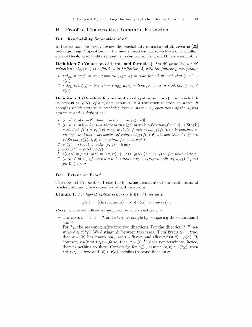
B Proof of Conservative Temporal Extension

B.1 Reachability Semantics of dL

In this section, we briefly review the reachability semantics of dL given in [20]before proving Proposition 1 in the next subsection. Here, we focus on the differ-ence of the dL reachability semantics in comparison to the dTL trace semantics.

Definition 7 (Valuation of terms and formulas). For dL formulas, the dLvaluation valdL(v, ·) is defined as in Definition 5, with the following exceptions:

1. valdL(v, [α]φ) = true :⇐⇒ valdL(w, φ) = true for all w such that (v, w) ∈ρ(α)

2. valdL(v, 〈α〉φ) = true :⇐⇒ valdL(w, φ) = true for some w such that (v, w) ∈ρ(α)

Definition 8 (Reachability semantics of system actions). The reachabil-ity semantics, ρ(α), of a system action α, is a transition relation on states. Itspecifies which state w is reachable from a state v by operations of the hybridsystem α and is defined as:

1. (v, w) ∈ ρ(x := θ) :⇐⇒ w = v[x 7→ valdL(v, θ)]2. (v, w) ∈ ρ(x = θ) :⇐⇒ there is an r ≥ 0 there is a function f : [0, r] → Sta(V )

such that f(0) = v, f(r) = w, and the function valdL(f(ζ), x) is continuouson [0, r] and has a derivative of value valdL(f(ζ), θ) at each time ζ ∈ (0, r),while valdL(f(ζ), y) is constant for each y 6= x

3. ρ(?χ) = {(v, v) : valdL(v, χ) = true}4. ρ(α ∪ γ) = ρ(α) ∪ ρ(γ)5. ρ(α; γ) = ρ(α)◦ρ(γ) = {(v, w) : (v, z) ∈ ρ(α), (z, w) ∈ ρ(γ) for some state z}6. (v, w) ∈ ρ(α∗) iff there are n ∈ N and v=v0, . . . , vn=w with (vi, vi+1) ∈ ρ(α)

for 0 ≤ i < n

B.2 Extension Proof

The proof of Proposition 1 uses the following lemma about the relationship ofreachability and trace semantics of dTL programs.

Lemma 1. For hybrid system actions α ∈ HP(V ), we have

ρ(α) = {(firstσ, lastσ) : σ ∈ τ(α) terminates} .

Proof. The proof follows an induction on the structure of α.

– The cases x := θ, x = θ, and α ∪ γ are simple by comparing the definitions 4and 8.

– For ?χ, the reasoning splits into two directions. For the direction “⊇”, as-sume σ ∈ τ(?χ). We distinguish between two cases. If val(firstσ, χ) = true,then σ = (v) has length one, lastσ = firstσ, and (firstσ, first σ) ∈ ρ(α). If,however, val(firstσ, χ) = false , then σ = (v, Λ) does not terminate, hence,there is nothing to show. Conversely, for “⊆”, assume (v, v) ∈ ρ(?χ), thenval(ν, χ) = true and (v) ∈ τ(α) satisfies the conditions on σ.

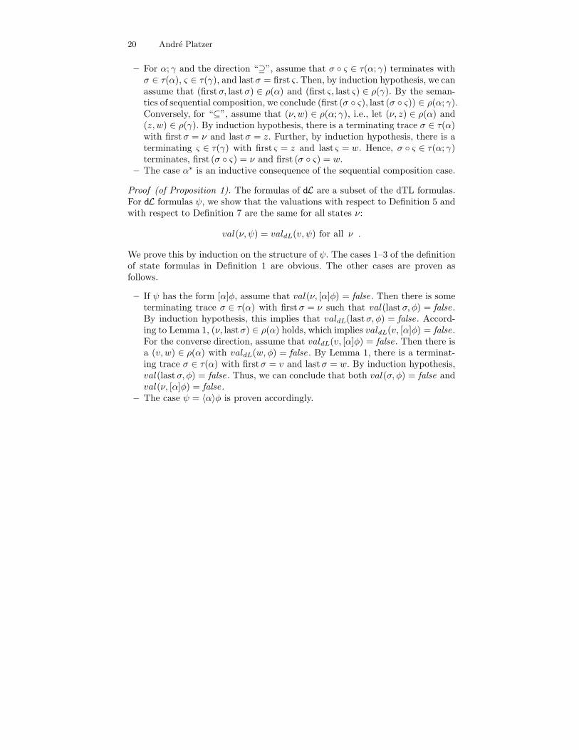
20 Andre Platzer

– For α; γ and the direction “⊇”, assume that σ ◦ ς ∈ τ(α; γ) terminates withσ ∈ τ(α), ς ∈ τ(γ), and lastσ = first ς. Then, by induction hypothesis, we canassume that (firstσ, lastσ) ∈ ρ(α) and (first ς, last ς) ∈ ρ(γ). By the seman-tics of sequential composition, we conclude (first (σ ◦ ς), last (σ ◦ ς)) ∈ ρ(α; γ).Conversely, for “⊆”, assume that (ν, w) ∈ ρ(α; γ), i.e., let (ν, z) ∈ ρ(α) and(z, w) ∈ ρ(γ). By induction hypothesis, there is a terminating trace σ ∈ τ(α)with firstσ = ν and lastσ = z. Further, by induction hypothesis, there is aterminating ς ∈ τ(γ) with first ς = z and last ς = w. Hence, σ ◦ ς ∈ τ(α; γ)terminates, first (σ ◦ ς) = ν and first (σ ◦ ς) = w.

– The case α∗ is an inductive consequence of the sequential composition case.

Proof (of Proposition 1). The formulas of dL are a subset of the dTL formulas.For dL formulas ψ, we show that the valuations with respect to Definition 5 andwith respect to Definition 7 are the same for all states ν:

val(ν, ψ) = valdL(v, ψ) for all ν .

We prove this by induction on the structure of ψ. The cases 1–3 of the definitionof state formulas in Definition 1 are obvious. The other cases are proven asfollows.

– If ψ has the form [α]φ, assume that val(ν, [α]φ) = false . Then there is someterminating trace σ ∈ τ(α) with firstσ = ν such that val(lastσ, φ) = false .By induction hypothesis, this implies that valdL(lastσ, φ) = false. Accord-ing to Lemma 1, (ν, lastσ) ∈ ρ(α) holds, which implies valdL(v, [α]φ) = false .For the converse direction, assume that valdL(v, [α]φ) = false. Then there isa (v, w) ∈ ρ(α) with valdL(w, φ) = false . By Lemma 1, there is a terminat-ing trace σ ∈ τ(α) with firstσ = v and lastσ = w. By induction hypothesis,val(lastσ, φ) = false . Thus, we can conclude that both val(σ, φ) = false andval(ν, [α]φ) = false .

– The case ψ = 〈α〉φ is proven accordingly.


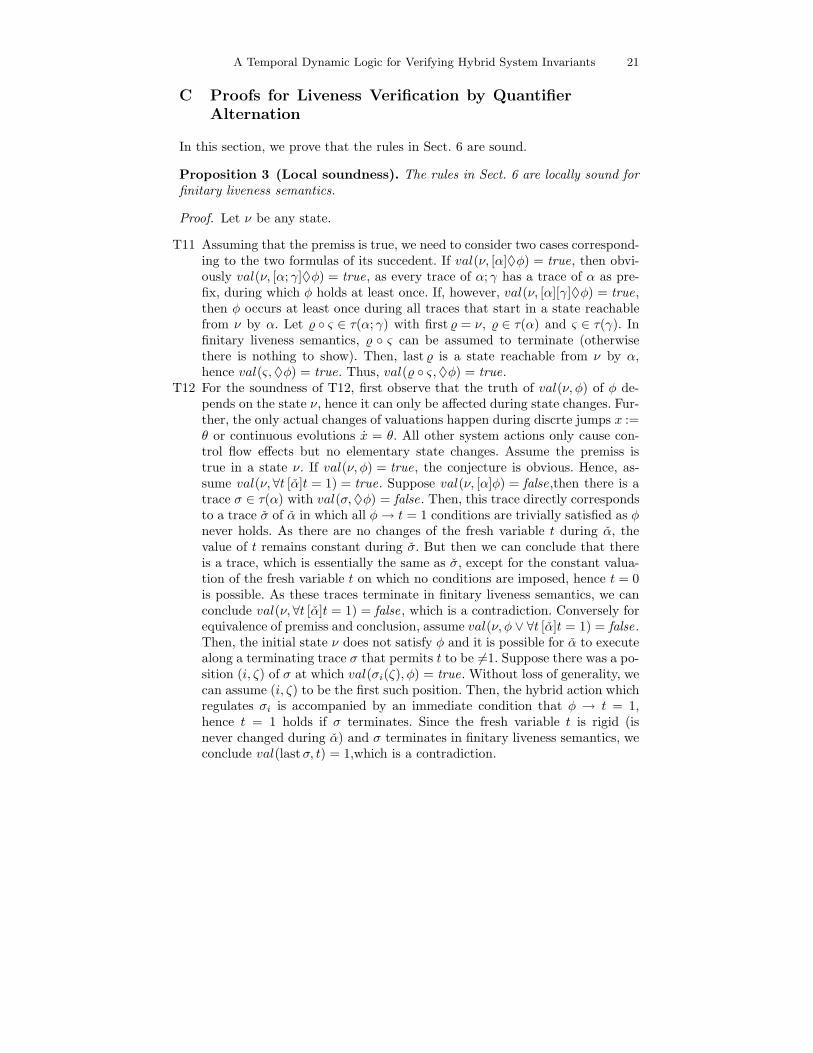
C Proofs for Liveness Verification by Quantifier

Alternation

In this section, we prove that the rules in Sect. 6 are sound.

Proposition 3 (Local soundness). The rules in Sect. 6 are locally sound forfinitary liveness semantics.

Proof. Let ν be any state.

T11 Assuming that the premiss is true, we need to consider two cases correspond-ing to the two formulas of its succedent. If val(ν, [α]♦φ) = true, then obvi-ously val(ν, [α; γ]♦φ) = true, as every trace of α; γ has a trace of α as pre-fix, during which φ holds at least once. If, however, val(ν, [α][γ]♦φ) = true,then φ occurs at least once during all traces that start in a state reachablefrom ν by α. Let ◦ ς ∈ τ(α; γ) with first = ν, ∈ τ(α) and ς ∈ τ(γ). Infinitary liveness semantics, ◦ ς can be assumed to terminate (otherwisethere is nothing to show). Then, last is a state reachable from ν by α,hence val(ς,♦φ) = true. Thus, val( ◦ ς,♦φ) = true.

T12 For the soundness of T12, first observe that the truth of val(ν, φ) of φ de-pends on the state ν, hence it can only be affected during state changes. Fur-ther, the only actual changes of valuations happen during discrte jumps x :=θ or continuous evolutions x = θ. All other system actions only cause con-trol flow effects but no elementary state changes. Assume the premiss istrue in a state ν. If val(ν, φ) = true, the conjecture is obvious. Hence, as-sume val(ν, ∀t [α]t = 1) = true. Suppose val(ν, [α]φ) = false,then there is atrace σ ∈ τ(α) with val(σ,♦φ) = false. Then, this trace directly correspondsto a trace σ of α in which all φ→ t = 1 conditions are trivially satisfied as φnever holds. As there are no changes of the fresh variable t during α, thevalue of t remains constant during σ. But then we can conclude that thereis a trace, which is essentially the same as σ, except for the constant valua-tion of the fresh variable t on which no conditions are imposed, hence t = 0is possible. As these traces terminate in finitary liveness semantics, we canconclude val(ν, ∀t [α]t = 1) = false , which is a contradiction. Conversely forequivalence of premiss and conclusion, assume val(ν, φ ∨ ∀t [α]t = 1) = false .Then, the initial state ν does not satisfy φ and it is possible for α to executealong a terminating trace σ that permits t to be 6=1. Suppose there was a po-sition (i, ζ) of σ at which val(σi(ζ), φ) = true. Without loss of generality, wecan assume (i, ζ) to be the first such position. Then, the hybrid action whichregulates σi is accompanied by an immediate condition that φ → t = 1,hence t = 1 holds if σ terminates. Since the fresh variable t is rigid (isnever changed during α) and σ terminates in finitary liveness semantics, weconclude val(lastσ, t) = 1,which is a contradiction.

REPORTS - AVACS: Start · A Temporal Dynamic Logic for Verifying Hybrid System Invariants by...

Documents

Transcript of REPORTS - AVACS: Start · A Temporal Dynamic Logic for Verifying Hybrid System Invariants by...