REPORTS A Large-Scale Deforestation … Large-Scale Deforestation Experiment: Effects of Patch ......
15
A Large-Scale Deforestation Experiment: Effects of Patch Area and Isolation on Amazon Birds Gonçalo Ferraz, 1 * James D. Nichols, 2 James E. Hines, 2 Philip C. Stouffer, 1,3 Richard O. Bierregaard Jr., 1,4 Thomas E. Lovejoy 1,5 As compared with extensive contiguous areas, small isolated habitat patches lack many species. Some species disappear after isolation; others are rarely found in any small patch, regardless of isolation. We used a 13-year data set of bird captures from a large landscape-manipulation experiment in a Brazilian Amazon forest to model the extinction-colonization dynamics of 55 species and tested basic predictions of island biogeography and metapopulation theory. From our models, we derived two metrics of species vulnerability to changes in isolation and patch area. We found a strong effect of area and a variable effect of isolation on the predicted patch occupancy by birds. T ropical forests are among the world’ s most threatened ecosystems, which are under severe pressure by human activ- ities, primarily deforestation (1). Deforestation reduces forest area and frequently isolates re- maining forest patches. Island biogeography (2) and metapopulation (3) theories predict the ef- fects of reduced area and increased isolation on rates of species extinction and colonization and thus on species occurrence. However, strong tests of these predictions are scarce. Most pub- lished inferences about the effects of area and isolation are based on patterns of species oc- currence, rather than directly on the dynamic rate parameters (such as extinction and coloni- zation) that produce these patterns. Multiple plausible hypotheses can be developed to ex- plain any such pattern, and pattern-based analy- ses thus produce weak inferences (4). The few studies that have focused on patch-occupancy dynamics follow observational, rather than ex- perimental, designs at small spatial and temporal scales, and they fail to deal adequately with detection probabilities: the fact that species may be present at a site yet go undetected. The Biological Dynamics of Forest Frag- ments Project (BDFFP) was initiated to test the effects of forest destruction at the patch level in a tropical ecosystem (5). The study, located in the central Brazilian Amazon, involved a reduction in forest area, which was predicted to increase the probabilities of local extinction of species, and isolation of remnant forest patches, which was predicted to reduce species colonization probabilities and increase extinction (2, 3, 6). The combined effects of both factors are pre- dicted to reduce patch occupancy (2, 3). We tested these predictions using data from the diverse bird community while separating infer- ences about area and isolation, in contrast to more usual approaches that confound these two effects as “fragmentation” (7). The data are of an experimental nature on relevant geographical and temporal scales, and our analysis treats de- tection probabilities explicitly. A mist-netting program monitored under- story birds in 23 primary-forest patches for 13 years (5). All patches were initially in continu- ous forest, but 11 of them were subsequently isolated by ranchland (two of which are depicted in Fig. 1). Patches were set in size classes of 1, 10, 100, 500, and 600 ha, with the largest iso- lated patch at 100 ha (table S1). The forest was cleared after monitoring began, permitting in- ference about the processes of extinction and colonization in isolated and continuous forest patches of different sizes (8). We used patch-occupancy models (9) to test a priori hypotheses about the influence of patch area and isolation on occurrence dynamics of 55 well-sampled bird species. The models contain four kinds of parameters: initial occu- pancy (y 1 ), local extinction probability (e), local probability of colonization (g), and prob- ability of detection given presence ( p). We limited our model set to plausible a priori hypotheses about the processes of detection, colonization, and local extinction, rather than conducting exploratory analyses with a larger model set including various combinations of potential covariates (table S2). y 1 is a free parameter and is never related to a covariate. p is a function of mist-netting effort and takes different values for different species. We pre- dicted that e would be related to patch area and isolation in one of three ways: a multiplicative function of patch size and isolation (full inter- action model), an additive function of the same two variables, and a function of patch size alone. g should be related to isolation, perhaps as mod- ified by regrowth of matrix habitat because some ranchland was abandoned. Colonization is modeled as a function of isolation, regrowth, and the “year 1 effect”—increased coloniza- tion by displaced birds immediately after deforestation—taken in five additive combina- tions. Isolation is a binary variable. We thus fitted 3 × 5 = 15 different models to each species using a maximum-likelihood approach in the program PRESENCE (10). Models were ranked by Akaike’ s information criterion (AIC) and AIC weight w j for model j (11). We predicted that patch size, independently of isolation, should have a negative effect on e (2, 3). Iso- lation, independently of size, should have a positive effect on local extinction via the reduc- tion of the “rescue effect” (6). We also asked three expert neotropical or- nithologists to classify the study species into two categories of dispersal ability (low and high). Isolation, through its effects on colonization and local extinction, should be more important for models of poor dispersers than for models of good dispersers. We expected forest regrowth to be more important for poor dispersers than for good dispersers. Among the variables that affect e and g, we predicted that dispersal ability would be the most relevant in the species’ responses to deforestation. Other variables may also be relevant, but their predicted effects are typically based on their relationship to dispersal ability. Thus, rather than testing the relevance of various species classification schemes, we focus here on our a priori prediction about the relevance of dispersal ability. 1 Biological Dynamics of Forest Fragments Project, Instituto Nacional de Pesquisas da Amazônia, 69011 Manaus AM, Brazil. 2 Patuxent Wildlife Research Center, Laurel, MD 20708, USA. 3 School of Renewable Natural Resources, Louisiana State University (LSU) and LSU AgCenter, Baton Rouge, LA 70803, USA. 4 Department of Biology, University of North Carolina, Charlotte, NC 28223, USA. 5 The H. John Heinz III Center for Science Economics and the Environ- ment, Washington, DC 20004, USA. *To whom correspondence should be addressed. E-mail: [email protected] Fig. 1. Two isolated fragments at Fazenda Dimona, Brazil. This aerial photograph of a 10-ha and a 1-ha frag- ment was taken shortly after isolation. Gaps between the fragment edge and the continu- ous forest are less than 1 km wide. 12 JANUARY 2007 VOL 315 SCIENCE www.sciencemag.org 238 REPORTS
Transcript of REPORTS A Large-Scale Deforestation … Large-Scale Deforestation Experiment: Effects of Patch ......
A Large-Scale DeforestationExperiment: Effects of Patch Areaand Isolation on Amazon BirdsGonçalo Ferraz,1* James D. Nichols,2 James E. Hines,2 Philip C. Stouffer,1,3Richard O. Bierregaard Jr.,1,4 Thomas E. Lovejoy1,5
As compared with extensive contiguous areas, small isolated habitat patches lack many species.Some species disappear after isolation; others are rarely found in any small patch, regardless ofisolation. We used a 13-year data set of bird captures from a large landscape-manipulationexperiment in a Brazilian Amazon forest to model the extinction-colonization dynamics of 55species and tested basic predictions of island biogeography and metapopulation theory. Fromour models, we derived two metrics of species vulnerability to changes in isolation and patch area.We found a strong effect of area and a variable effect of isolation on the predicted patchoccupancy by birds.
Tropical forests are among the world’smost threatened ecosystems, which areunder severe pressure by human activ-
ities, primarily deforestation (1). Deforestationreduces forest area and frequently isolates re-maining forest patches. Island biogeography (2)and metapopulation (3) theories predict the ef-fects of reduced area and increased isolation onrates of species extinction and colonization andthus on species occurrence. However, strongtests of these predictions are scarce. Most pub-lished inferences about the effects of area andisolation are based on patterns of species oc-currence, rather than directly on the dynamicrate parameters (such as extinction and coloni-zation) that produce these patterns. Multipleplausible hypotheses can be developed to ex-plain any such pattern, and pattern-based analy-ses thus produce weak inferences (4). The fewstudies that have focused on patch-occupancydynamics follow observational, rather than ex-perimental, designs at small spatial and temporalscales, and they fail to deal adequately withdetection probabilities: the fact that species maybe present at a site yet go undetected.
The Biological Dynamics of Forest Frag-ments Project (BDFFP) was initiated to test theeffects of forest destruction at the patch level in atropical ecosystem (5). The study, located in thecentral Brazilian Amazon, involved a reductionin forest area, which was predicted to increasethe probabilities of local extinction of species,and isolation of remnant forest patches, whichwas predicted to reduce species colonizationprobabilities and increase extinction (2, 3, 6).The combined effects of both factors are pre-
dicted to reduce patch occupancy (2, 3). Wetested these predictions using data from thediverse bird community while separating infer-ences about area and isolation, in contrast tomore usual approaches that confound these twoeffects as “fragmentation” (7). The data are of anexperimental nature on relevant geographicaland temporal scales, and our analysis treats de-tection probabilities explicitly.
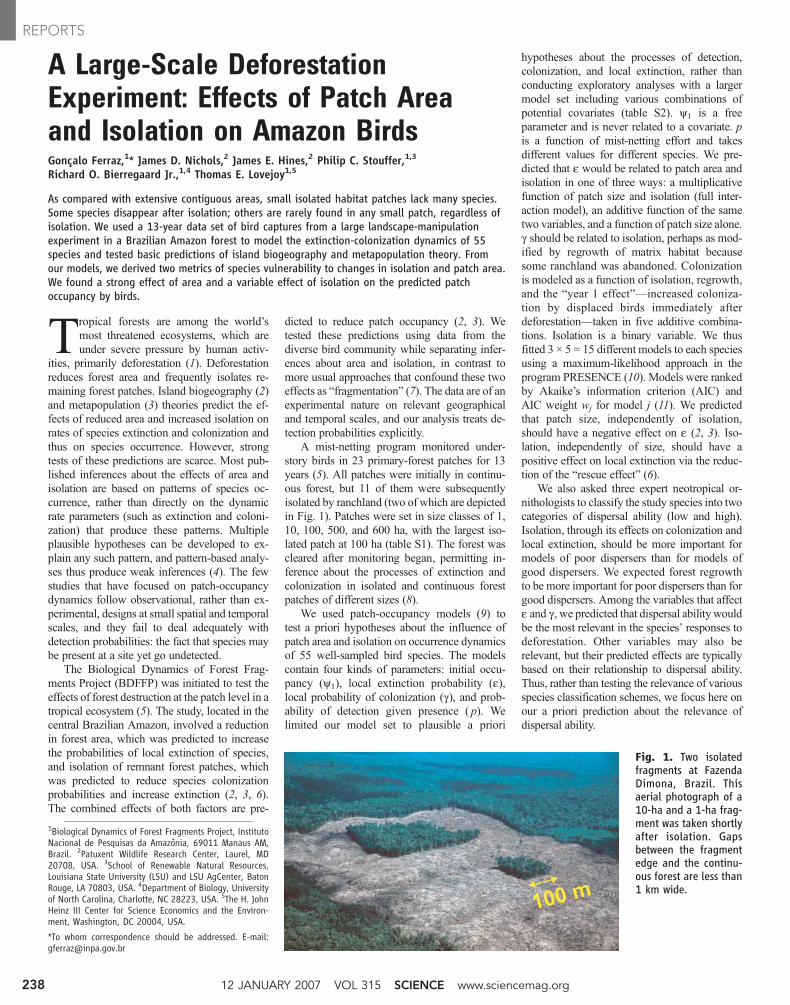
A mist-netting program monitored under-story birds in 23 primary-forest patches for 13years (5). All patches were initially in continu-ous forest, but 11 of them were subsequentlyisolated by ranchland (two of which are depictedin Fig. 1). Patches were set in size classes of 1,10, 100, 500, and 600 ha, with the largest iso-lated patch at 100 ha (table S1). The forest wascleared after monitoring began, permitting in-ference about the processes of extinction andcolonization in isolated and continuous forestpatches of different sizes (8).
We used patch-occupancy models (9) totest a priori hypotheses about the influence ofpatch area and isolation on occurrence dynamicsof 55 well-sampled bird species. The modelscontain four kinds of parameters: initial occu-pancy (y1), local extinction probability (e),local probability of colonization (g), and prob-ability of detection given presence ( p). Welimited our model set to plausible a priori
hypotheses about the processes of detection,colonization, and local extinction, rather thanconducting exploratory analyses with a largermodel set including various combinations ofpotential covariates (table S2). y1 is a freeparameter and is never related to a covariate. pis a function of mist-netting effort and takesdifferent values for different species. We pre-dicted that e would be related to patch area andisolation in one of three ways: a multiplicativefunction of patch size and isolation (full inter-action model), an additive function of the sametwo variables, and a function of patch size alone.g should be related to isolation, perhaps as mod-ified by regrowth of matrix habitat becausesome ranchland was abandoned. Colonizationis modeled as a function of isolation, regrowth,and the “year 1 effect”—increased coloniza-tion by displaced birds immediately afterdeforestation—taken in five additive combina-tions. Isolation is a binary variable. We thusfitted 3 × 5 = 15 different models to each speciesusing a maximum-likelihood approach in theprogram PRESENCE (10). Models were rankedby Akaike’s information criterion (AIC) andAIC weight wj for model j (11). We predictedthat patch size, independently of isolation,should have a negative effect on e (2, 3). Iso-lation, independently of size, should have apositive effect on local extinction via the reduc-tion of the “rescue effect” (6).
We also asked three expert neotropical or-nithologists to classify the study species into twocategories of dispersal ability (low and high).Isolation, through its effects on colonization andlocal extinction, should be more important formodels of poor dispersers than for models ofgood dispersers. We expected forest regrowthto be more important for poor dispersers than forgood dispersers. Among the variables that affecte and g, we predicted that dispersal ability wouldbe the most relevant in the species’ responses todeforestation. Other variables may also berelevant, but their predicted effects are typicallybased on their relationship to dispersal ability.Thus, rather than testing the relevance of variousspecies classification schemes, we focus here onour a priori prediction about the relevance ofdispersal ability.
1Biological Dynamics of Forest Fragments Project, InstitutoNacional de Pesquisas da Amazônia, 69011 Manaus AM,Brazil. 2Patuxent Wildlife Research Center, Laurel, MD20708, USA. 3School of Renewable Natural Resources,Louisiana State University (LSU) and LSU AgCenter, BatonRouge, LA 70803, USA. 4Department of Biology, Universityof North Carolina, Charlotte, NC 28223, USA. 5The H. JohnHeinz III Center for Science Economics and the Environ-ment, Washington, DC 20004, USA.
*To whom correspondence should be addressed. E-mail:[email protected]
Fig. 1. Two isolatedfragments at FazendaDimona, Brazil. Thisaerial photograph of a10-ha and a 1-ha frag-ment was taken shortlyafter isolation. Gapsbetween the fragmentedge and the continu-ous forest are less than1 km wide.
12 JANUARY 2007 VOL 315 SCIENCE www.sciencemag.org238
REPORTS
Our analysis follows three steps, all of whichare based on fitting models for each species.First, we ask what covariates appear in the top-ranking models of each species. Second, wefocus on the single model that fits best acrossspecies and examine the signs and magnitudesof covariate effects (slope parameters). Finally,we select one best-fitting model per species anddraw inferences based on the estimated localextinction and colonization parameters.
Patch isolation appears as a covariate ofcolonization and/or local extinction in high-ranking models (wj > 0.2) of nearly all, but notall, species (Table 1 and table S3). Patch size,regardless of isolation, seems sufficient toexplain the observations on three exceptionspecies: Geotrygon montana, Dendrocolaptescerthia, and Hypocnemis cantator. Fifteen spe-cies have high-ranking models with an effect ofisolation only on local extinction, and fivespecies have high-ranking models with thateffect only on colonization. Regrowth entershigh-ranking models in two-fifths of the species.Contrary to our expectation, we cannot reject thenull hypothesis that regrowth enters high-ranking models of high- and low-dispersalspecies in the same proportions (one-tailed ztest, P = 0.33). Likewise, there is no evidence tosustain the prediction that isolation would ap-pear more frequently in high-ranking models oflow-dispersal species (one-tailed z test, P= 0.97).Inferences are qualitatively the same if high-ranking models are redefined as having wj >0.1 or wj > 0.25.
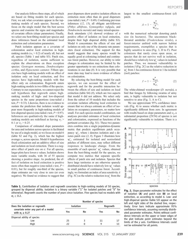
Comparison of estimated slope parametersfor area and isolation across species is facilitatedby use of a singlemodel, sowe focus onmodel 6(table S2 and Fig. 2), which has the highestaverage wj across species. Model 6 hypothesizesfixed colonization and an additive effect of sizeand isolation on local extinction. There is a neg-ative effect of patch size on e: For all species,larger plots have lower e values. Isolation showsmore variable results, with 36 of 55 speciesshowing a positive slope. As predicted, the ef-fect of isolation on local extinction is positivemore often than negative (one-tailed z test, P <0.01), but for roughly one-third of the species,slope estimates are very close to zero (or evennegative). We found no evidence to suggest that
poor dispersers show positive isolation effects onextinction more often than do good dispersers(one-tailed z test, P = 0.49). Confirming previousinferences (12, 13), all obligate ant-followers(Pithys albifrons, Gymnopithys rufigula, andDendrocincla merula) and many mixed-species–flock attendants (14) showed evidence of apositive effect of isolation on local extinction,despite their high dispersal ability (table S3).Model 6 concentrates the effects of size andisolation on only one of the dynamic rate param-eters (local extinction). The support for thismodel suggests that many species would beequally good at colonizing isolated and continu-ous forest patches. However, our ability to inferchanges in colonization may be limited by thegreater opportunity to see extinctions than colo-nizations in our data (8). It is very possible thatmore data may lead to more evidence of effectson colonization.
By selecting the best-fitting model for eachspecies, we can account for the effect ofregrowth and for the possible interaction be-tween the effects of size and isolation on localextinction (table S4) (8), which are two aspectsthat model 6 did not address. We select onlyfrom the subset of 10 models that includes thecovariate isolation affecting local extinction toensure that we always estimate an effect of iso-lation on occupancy parameters, no matter howsmall. For each species-model combination, ouranalyses provided estimates of local extinctionand colonization, expressed as functions of thepertinent covariates (fig. S1). These two param-eters combine into a single population-dynamicmetric that predicts equilibrium patch occu-pancy y�
is, where i denotes isolation and s de-
notes patch size (3, 8). Figure 3 illustrates howy�is, estimated for isolated and nonisolated
patches of different sizes, may reflect differentresponses to landscape change. From theensemble of each species’ y�
isvalues, obtained
from the best-fitting model for the species, wecompute two metrics that separate specificeffects of patch size and isolation. Species thathave large territories or are otherwise sparselydistributed should have relatively lowy�
isvalues
in small patches of continuous forest. Accord-ingly, we formulate an index of area sensitivityA(Fig. 3C) as the relative reduction iny�
isfrom the
largest to the smallest continuous-forest (cf)patch:
A ¼ 1 −y*cf1y*cf100
ð1Þ
with the numerical subscript denoting patchsize (in hectares). The uncommon black-throated antshrike (Frederickena viridis), aforest-interior antbird with narrow habitatrequirements, exemplifies a species that ishighly sensitive to area (Fig. 3, D to F). Poorcolonizers that rarely cross open areas, orspecies that do not survive well in isolation,should have relatively lowy�
isvalues in isolated
patches. Thus, we measure vulnerability toisolation I (Fig. 2C) as the relative reduction iny�isfrom 1-ha continuous-forest to 1-ha isolated
(isol) patches:
I ¼ 1 −y*isol1y*cf1
ð2Þ
The white-chinned woodcreeper (D. merula), abird that forages by following swarms of armyants, is highly vulnerable to isolation but notsensitive to area (Fig. 3, A to C).
We use approximate 95% confidence inter-vals (Fig. 4) to assess whether each metric issignificantly different from zero. In agreementwith results based on slope parameters and wj, asubstantial proportion (29/54) of species is notsignificantly vulnerable to isolation. There is a
Table 1. Contribution of isolation and regrowth covariates to high-ranking models of 50 species,grouped by dispersal ability. Isolation is a binary variable (“1” for isolated patches and “0” forotherwise). Regrowth counts the number of years since isolation. Five species had no models withwj ≥ 0.2.
Number of species
Does the isolation or regrowthcovariate enter any part of a modelwith wj ≥ 0.2?
Isolation Regrowth
Yes No Yes No
Dispersal ability of speciesLow 25 3 11 17High 22 0 9 13
–10
0
10
20
30Is
olat
ion
slop
eA
–30
–20
–10
0
10
Siz
e sl
ope
species
B
Fig. 2. Slope parameter estimates for the effectof isolation (A) and patch size (B) on localextinction, as according to model 6. Low- andhigh-dispersal species (table S3) appear on theleft and right sides of the dashed line, respec-tively. Error bars indicate approximate 95%confidence intervals, assuming normally distrib-uted parameter estimates. Points without confi-dence intervals on the upper or lower edges ofthe plot indicate point estimates beyond thelimits of the y axis. Confidence intervals couldnot be estimated for all points.
www.sciencemag.org SCIENCE VOL 315 12 JANUARY 2007 239
REPORTS
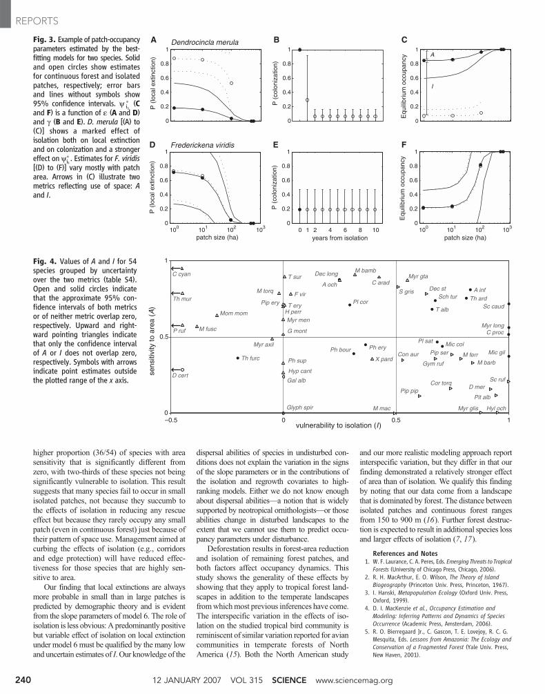
higher proportion (36/54) of species with areasensitivity that is significantly different fromzero, with two-thirds of these species not beingsignificantly vulnerable to isolation. This resultsuggests that many species fail to occur in smallisolated patches, not because they succumb tothe effects of isolation in reducing any rescueeffect but because they rarely occupy any smallpatch (even in continuous forest) just because oftheir pattern of space use. Management aimed atcurbing the effects of isolation (e.g., corridorsand edge protection) will have reduced effec-tiveness for those species that are highly sen-sitive to area.
Our finding that local extinctions are alwaysmore probable in small than in large patches ispredicted by demographic theory and is evidentfrom the slope parameters of model 6. The role ofisolation is less obvious: A predominantly positivebut variable effect of isolation on local extinctionunder model 6 must be qualified by the many lowand uncertain estimates of I. Our knowledge of the
dispersal abilities of species in undisturbed con-ditions does not explain the variation in the signsof the slope parameters or in the contributions ofthe isolation and regrowth covariates to high-ranking models. Either we do not know enoughabout dispersal abilities—a notion that is widelysupported by neotropical ornithologists—or thoseabilities change in disturbed landscapes to theextent that we cannot use them to predict occu-pancy parameters under disturbance.
Deforestation results in forest-area reductionand isolation of remaining forest patches, andboth factors affect occupancy dynamics. Thisstudy shows the generality of these effects byshowing that they apply to tropical forest land-scapes in addition to the temperate landscapesfromwhichmost previous inferences have come.The interspecific variation in the effects of iso-lation on the studied tropical bird community isreminiscent of similar variation reported for aviancommunities in temperate forests of NorthAmerica (15). Both the North American study
and our more realistic modeling approach reportinterspecific variation, but they differ in that ourfinding demonstrated a relatively stronger effectof area than of isolation. We qualify this findingby noting that our data come from a landscapethat is dominated by forest. The distance betweenisolated patches and continuous forest rangesfrom 150 to 900 m (16). Further forest destruc-tion is expected to result in additional species lossand larger effects of isolation (7, 17).
References and Notes1. W. F. Laurance, C. A. Peres, Eds. Emerging Threats to Tropical
Forests (University of Chicago Press, Chicago, 2006).2. R. H. MacArthur, E. O. Wilson, The Theory of Island
Biogeography (Princeton Univ. Press, Princeton, 1967).3. I. Hanski, Metapopulation Ecology (Oxford Univ. Press,
Oxford, 1999).4. D. I. MacKenzie et al., Occupancy Estimation and
Modeling: Inferring Patterns and Dynamics of SpeciesOccurrence (Academic Press, Amsterdam, 2006).
5. R. O. Bierregaard Jr., C. Gascon, T. E. Lovejoy, R. C. G.Mesquita, Eds. Lessons from Amazonia: The Ecology andConservation of a Fragmented Forest (Yale Univ. Press,New Haven, 2001).
Fig. 3. Example of patch-occupancyparameters estimated by the best-fitting models for two species. Solidand open circles show estimatesfor continuous forest and isolatedpatches, respectively; error barsand lines without symbols show95% confidence intervals. y �
is (Cand F) is a function of e (A and D)and g (B and E). D. merula [(A) to(C)] shows a marked effect ofisolation both on local extinctionand on colonization and a strongereffect ony�
is . Estimates for F. viridis[(D) to (F)] vary mostly with patcharea. Arrows in (C) illustrate twometrics reflecting use of space: Aand I.
0
0.2
0.4
0.6
0.8
1Dendrocincla merula
100 101 102 103
patch size (ha)
Frederickena viridis
0 1 2 4 6 8 10years from isolation patch size (ha)
A B C
FED
A
I
P (
loca
l ext
inct
ion)
P (
loca
l ext
inct
ion)
P (
colo
niza
tion)
P (
colo
niza
tion)
Equ
ilibr
ium
occ
upan
cyE
quili
briu
m o
ccup
ancy
0
0.2
0.4
0.6
0.8
1
0
0.2
0.4
0.6
0.8
1
0
0.2
0.4
0.6
0.8
1
0
0.2
0.4
0.6
0.8
1
0
0.2
0.4
0.6
0.8
1
100 101 102 103
Fig. 4. Values of A and I for 54species grouped by uncertaintyover the two metrics (table S4).Open and solid circles indicatethat the approximate 95% con-fidence intervals of both metricsor of neither metric overlap zero,respectively. Upward and right-ward pointing triangles indicatethat only the confidence intervalof A or I does not overlap zero,respectively. Symbols with arrowsindicate point estimates outsidethe plotted range of the x axis.
Th ard
T alb
Dec long
Ph bour
Myr long
A inf
Pl sat
Sch turPl cor
Mic colPh eryMic gil
Dec st
C proc
Th furc
Sc caud
Con aur
Cor torqD mer
Gym ruf
Hyl ochM mac
M barb
Pip ser
Myr glis
Pip pip
M ferr
Pit alb
Sc ruf
A och
C cyan
C arad
F vir
G mont
H perr
Hyp cant
M fusc
M bamb
Mom mom
M torq
Myr axil
Myr gta
Myr men
P ruf
Ph sup
Pip ery
S gris
X pard
T ery
T sur
Th mur
D certGal alb
Glyph spir0
0.5
1
–0.5 0 0.5 1vulnerability to isolation (I)
sens
itivi
ty to
are
a (A
)
12 JANUARY 2007 VOL 315 SCIENCE www.sciencemag.org240
REPORTS
6. J. H. Brown, A. Kodric-Brown, Ecology 58, 445 (1977).7. L. Fahrig, Annu. Rev. Ecol. Evol. Syst. 34, 487 (2003).8. Materials and methods are available as supporting
material on Science Online.9. D. I. MacKenzie, J. D. Nichols, J. E. Hines, M. G. Knutson,
A. B. Franklin, Ecology 84, 2200 (2003).10. J. E. Hines, PRESENCE version 2.0 (computer program),
U.S. Geological Survey, Patuxent Wildlife ResearchCenter, Laurel, MD (2004).
11. K. P. Burnham, D. R. Anderson, Model Selection andMultimodel Inference: A Practical Information-TheoreticApproach (Springer, New York, 2002).
12. P. C. Stouffer, R. O. Bierregaard Jr., Ecology 76, 2429 (1995).
13. K. S. Van Houtan, S. L. Pimm, R. O. Bierregaard Jr.,T. E. Lovejoy, P. C. Stouffer, Evol. Ecol. Res. 8, 129(2006).
14. M. Cohn-Haft, A. Whittaker, P. C. Stouffer, Ornithol.Monogr. 48, 205 (1997).
15. C. S. Robbins, D. K. Dawson, B. A. Dowell, Wildl. Monogr.103, 1 (1989).
16. C. Gascon, R. O. Bierregaard Jr., in (5), pp. 31–45.17. M. K. Trzcinski, L. Fahrig, G. Merriam, Ecol. Appl. 9, 586
(1999).18. We thank A. Whittaker, J.-M. Thiollay, and S. Borges for
help with classification of dispersal abilities. L. Naka andM. Cohn-Haft provided key natural history information.
G.F. was supported by BDFFP funds and a ConselhoNacional de Desenvolvimento Científico e Tecnológico(Brazilian Government) grant. This is BDFFP technicalseries contribution number 473.
Supporting Online Materialwww.sciencemag.org/cgi/content/full/315/5809/238/DC1Materials and MethodsFig. S1Tables S1 to S4References
27 July 2006; accepted 28 November 200610.1126/science.1133097
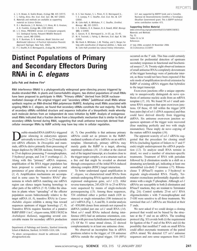
Distinct Populations of Primaryand Secondary Effectors DuringRNAi in C. elegansJulia Pak and Andrew Fire*
RNA interference (RNAi) is a phylogenetically widespread gene-silencing process triggered bydouble-stranded RNA. In plants and Caenorhabditis elegans, two distinct populations of small RNAshave been proposed to participate in RNAi: “Primary siRNAs” (derived from DICER nuclease-mediated cleavage of the original trigger) and “secondary siRNAs” [additional small RNAs whosesynthesis requires an RNA-directed RNA polymerase (RdRP)]. Analyzing small RNAs associated withongoing RNAi in C. elegans, we found that secondary siRNAs constitute the vast majority. The bulkof secondary siRNAs exhibited structure and sequence indicative of a biosynthetic mode wherebyeach molecule derives from an independent de novo initiation by RdRP. Analysis of endogenoussmall RNAs indicated that a fraction derive from a biosynthetic mechanism that is similar to that ofsecondary siRNAs formed during RNAi, suggesting that small antisense transcripts derived fromcellular messenger RNAs by RdRP activity may have key roles in cellular regulation.
Double-strandedRNA (dsRNA)–triggeredgene silencing in eukaryotes appearsuniversally to involve 21- to 25-nucleotide
(nt) siRNA effectors. In Drosophila and mam-mals, siRNAs derive primarily from processing oflonger duplexes by DICER nuclease, forming 21-to 25-nt duplexes possessing 5′-monophosphates,3′-hydroxyl groups, and 2-nt 3′ overhangs (1, 2).Along with this “primary” siRNA response,amplification of the RNA trigger population hasbeen proposed to contribute to potency andpersistence of gene silencing in several systems(3, 4). Amplification mechanisms are accompa-nied in some cases by “transitive RNAi” phe-nomena in which dsRNA matching one mRNAregion can silence targets bearing homology toother parts of the mRNA (5–9). Unlike the situa-tion in plants where “spreading” of the effectorpopulation occurs bidirectionally relative to thetarget mRNA (6, 8), transitive RNAi in Caeno-rhabditis elegans exhibits a strong bias towardsequences upstream of trigger homology (7, 9).Transitive RNAi requires function of a putativeRdRP (RRF-1 inC. elegans soma, SDE1/SGS2 inArabidopsis thaliana), suggesting several con-ceivable means for secondary siRNA production
(6, 7). One possibility is that antisense primarysiRNAs could act as primers in the RdRP-mediated synthesis of new dsRNAs on an mRNAtemplate. Alternatively, primary siRNAs maymerely guide the RdRP to a target, allowingunprimed synthesis (10, 11) either at the cleavedend of the targeted transcript, at a location close tothe trigger-target complex, or at a structure such asa free end that might be revealed as aberrantthrough consequences of the initial RNA-inducedsilencing complex (RISC)::target interaction.
To better understand signal amplification inC. elegans, we characterized small RNAs fromanimals undergoing RNAi against an abundantlyexpressed endogenous gene, sel-1 (12). Afterreverse transcription, 245,420 18- to 25-nt RNAswere sequenced by means of single-moleculepyrosequencing (13). Among these sequences,534 exhibited either a perfect match (428 in-stances) or single mismatches (106 instances) tosel-1mRNA (Fig. 1, A and B). A similar analysisof ~850,000 clones from animals not exposed todsRNA yielded just one sel-1 small RNA (14).Most sel-1 small RNAs induced during inter-ference (483) had an antisense orientation, con-sistent with previous hybridization-based analyses(7). Of the 51 sense strand clones, 22 showedcomplementarity to at least one antisense clone.
We observed an incomplete bias in siRNApositions relative to the trigger; of 138 antisensesiRNAs outside the original trigger, 110 (80%)
occurred on the 5′ side. This bias could certainlyaccount for preferential detection of upstreamsecondary responses in functional and biochemi-cal assays (7, 9). Twenty-eight observed instancesof small antisense RNAs completely downstreamof the trigger homology were of particular inter-est, as these would not have been expected if thesole mode of amplification involved extension byRdRP of existing siRNA triggers that hybridizeto the target transcript.
Exon-exon junctions offer a unique opportu-nity to unequivocally distinguish de novo syn-thesis of antisense nucleic acids from an mRNAtemplate (15, 16). We found 50 sel-1 small anti-sense RNA sequences that span exon/exon junc-tions. Of these, 43 fall within the trigger [458base pairs (bp) of sel-1 cDNA sequence] and thuscould have derived directly from triggeringdsRNA. Six antisense exon-exon junction se-quences upstream of the trigger were recovered(four matching perfectly and two with singlemismatches). These imply de novo copying ofthe mature mRNA template (16).
The apparent scarcity of sel-1 siRNAs sug-gested that the procedure for cloning smallRNAs (including ligation of linkers to 3′ and 5′ends) might underrepresent the siRNA popula-tion (12). To analyze small RNA termini indetail, we used a number of structure-specifictreatments. Treatment of RNA with periodatefollowed by b elimination results in a shift on adenaturing acrylamide gel, indicating at least oneunmodified (cis-diol) 3′ terminus (17). Ribonu-clease T (RNaseT) requires a 3′-hydroxyl todegrade single-stranded RNA. Finally, Ter-minator exonuclease preferentially degrades sub-strates with a single 5′-phosphate. Although sel-1siRNAs are susceptible to both b elimination andRNaseT reactions, they are resistant to Terminator(Fig. 2A). Control synthetic 25-nt sel-1 RNAoligonucleotides s with 5′-monophosphate and3′-OH were sensitive to all three treatments. Wesurmised that sel-1 siRNAs are blocked at their5′ ends.
We next asked if we could design a cloningprotocol that would not be biased by the struc-ture at the 5′ end on an siRNA. The resultingprotocol (fig. S3) avoids both (i) the requirementfor ligation of the 5′ end of the RNA and (ii) thepossibility that modified 5′ ends on small RNAscould affect enzymatic treatments of the pairedcDNA strand. We detected 127 sel-1 antisensesequences and zero sense sequences from 1612
Departments of Pathology and Genetics, Stanford UniversitySchool of Medicine, Stanford, CA 94305–5324, USA.
*To whom correspondence should be addressed. E-mail:[email protected]
www.sciencemag.org SCIENCE VOL 315 12 JANUARY 2007 241
REPORTS
www.sciencemag.org/cgi/content/full/315/5809/238/DC1
Supporting Online Material for
A Large-Scale Deforestation Experiment:
Effects of Patch Area and Isolation on Amazon Birds
Gonçalo Ferraz,* James D. Nichols, James E. Hines, Philip C. Stouffer, Richard O. Bierregaard Jr., Thomas E. Lovejoy
*To whom correspondence should be addressed. E-mail: [email protected]
Published 12 January 2007, Science 315, 238 (2007)
DOI: 10.1126/science.1133097
This PDF file includes:
Materials and Methods Fig. S1 Tables S2 to S4 References
Other Supporting Online Material for this manuscript includes the following: (available at www.sciencemag.org/cgi/content/full/315/5809/238/DC1)
Table S1 as a zipped archive
Material and methods
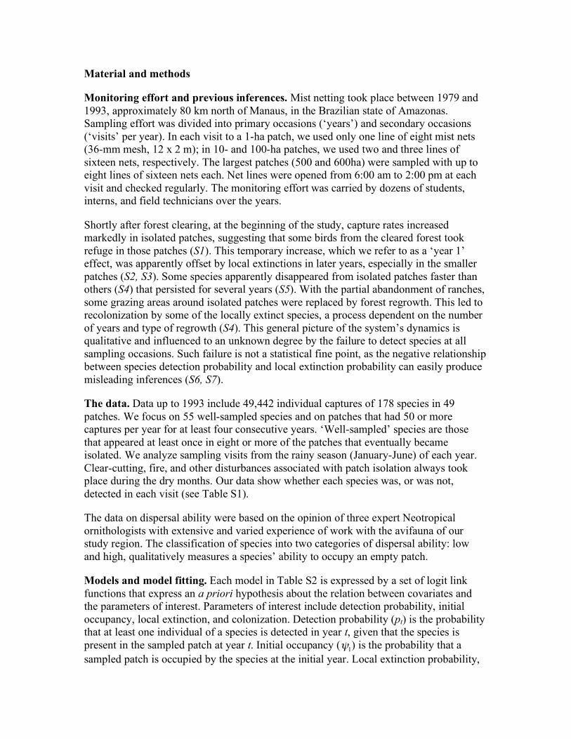
Monitoring effort and previous inferences. Mist netting took place between 1979 and 1993, approximately 80 km north of Manaus, in the Brazilian state of Amazonas. Sampling effort was divided into primary occasions (‘years’) and secondary occasions (‘visits’ per year). In each visit to a 1-ha patch, we used only one line of eight mist nets (36-mm mesh, 12 x 2 m); in 10- and 100-ha patches, we used two and three lines of sixteen nets, respectively. The largest patches (500 and 600ha) were sampled with up to eight lines of sixteen nets each. Net lines were opened from 6:00 am to 2:00 pm at each visit and checked regularly. The monitoring effort was carried by dozens of students, interns, and field technicians over the years.
Shortly after forest clearing, at the beginning of the study, capture rates increased markedly in isolated patches, suggesting that some birds from the cleared forest took refuge in those patches (S1). This temporary increase, which we refer to as a ‘year 1’ effect, was apparently offset by local extinctions in later years, especially in the smaller patches (S2, S3). Some species apparently disappeared from isolated patches faster than others (S4) that persisted for several years (S5). With the partial abandonment of ranches, some grazing areas around isolated patches were replaced by forest regrowth. This led to recolonization by some of the locally extinct species, a process dependent on the number of years and type of regrowth (S4). This general picture of the system’s dynamics is qualitative and influenced to an unknown degree by the failure to detect species at all sampling occasions. Such failure is not a statistical fine point, as the negative relationship between species detection probability and local extinction probability can easily produce misleading inferences (S6, S7).
The data. Data up to 1993 include 49,442 individual captures of 178 species in 49 patches. We focus on 55 well-sampled species and on patches that had 50 or more captures per year for at least four consecutive years. ‘Well-sampled’ species are those that appeared at least once in eight or more of the patches that eventually became isolated. We analyze sampling visits from the rainy season (January-June) of each year. Clear-cutting, fire, and other disturbances associated with patch isolation always took place during the dry months. Our data show whether each species was, or was not, detected in each visit (see Table S1).
The data on dispersal ability were based on the opinion of three expert Neotropical ornithologists with extensive and varied experience of work with the avifauna of our study region. The classification of species into two categories of dispersal ability: low and high, qualitatively measures a species’ ability to occupy an empty patch.
Models and model fitting. Each model in Table S2 is expressed by a set of logit link functions that express an a priori hypothesis about the relation between covariates and the parameters of interest. Parameters of interest include detection probability, initial occupancy, local extinction, and colonization. Detection probability (pt) is the probability that at least one individual of a species is detected in year t, given that the species is present in the sampled patch at year t. Initial occupancy (
!
"1) is the probability that a
sampled patch is occupied by the species at the initial year. Local extinction probability,
(εt) is the probability that a patch occupied by the species at year t is no longer occupied by the species at year t+1. Local probability of colonization (γt) is the probability that a patch not occupied by the species at year t is occupied at year t+1. For simplicity, we drop the time indexes on p, ε, and γ here, and in the manuscript.
We model
!
"1 as a free parameter, never related to a covariate. Detection (p) takes
different values for different species and is a function of effort alone, with effort measured in net*hours per visit. Time- and patch-specific probabilities of local extinction (ε) and colonization (γ) are functions of up to five patch covariates: patch size, isolation, ‘year 1’, regrowth, and ‘late regrowth’ (see Table S2). Patch size (ha) does not change through time. Isolation and ‘year 1’ are binary variables that take the value ‘1’ in the case of isolation and in the first year after isolation, respectively. Regrowth and ‘late regrowth’ count the number of years since isolation, starting respectively, at year one and year two; the counting restarts every time a patch is re-isolated.
Just as in classic island biogeography (S8) and many metapopulation (S9) models, we hypothesize that colonization may be affected by isolation, but not by area. Our treatment of extinction, however, differs from many classic models (S9, S10) in admitting that isolation, and not just area, may contribute to the probability of extinction. We believe that species occasionally avoid local extinction through the arrival of immigrants, or they may go extinct from, and later re-colonize a patch between two consecutive samples (S11). If this ‘rescue effect’ is embedded in the data, our observation of extinction (or lack of it) should be affected by isolation and by area, because it would reflect a combination of both extinction and colonization processes. This is why we chose to model local extinction as a function of both area and isolation.
In developing the set of a priori models, our task was to settle on a small number of models that included the most important potential effects on quantities of interest. This limitation of the model set (S12) is not the only approach to scientific learning, but is one that seems reasonable to us. We elected to model p as a function of effort alone. Effort was the most obvious covariate for the modeling of detection probability. Indeed, an entire class of models (catch-effort) used to estimate animal abundance and survival is based on the relationship between effort and detection probability (S13). Other covariates might arguably influence detection as well, but the rationale for the importance of effort (net*hours) on probability of detection is far stronger than for any other covariate that we could measure. Isolation, time, and rainfall were all plausible candidate covariates. Initial modelling of isolation on a subset of species produced discouraging results, however, thanks to poor model fits (providing little evidence that isolation was relevant to detection probability) and parameter identifiability problems. Time is most likely to affect detection due to temporal variations in effort – already expressed in the effort covariate. Finally, we could not model the effect of rainfall because we do not have daily information on this or any other weather variable. We thus became convinced that adding more covariates to the detection model would substantially increase the size and complexity of the model set without a comparable improvement in the interpretation of our data.
Apart from comparing models from an a priori model set, we also compare species by focusing on the slope parameter estimates from one same model fitted to every species. For this purpose, we chose Model 6, because it had the highest AIC weight (see next paragraph) across species. Model 6 hypothesises an additive effect of isolation and area on local extinction, and a fixed probability of colonization, unaffected by patch isolation. Why would such a simple model provide an adequate explanation of variation in our data? We do believe that many species cross the relatively open land that surrounds isolated patches, and thus have the ability to colonize isolated as well as continuous forest sites. However, our ability to infer any changes in colonization may be limited by (1) the greater opportunity to see extinctions than colonizations in our data (occupancy is conditional on patch state, and the “occupied” state was much more common than “unoccupied” for many species, especially at the beginning of the study) and (2) the generally greater difficulty in estimating quantities that are conditional on a state that cannot be directly observed, in this case the unoccupied state.
We use program PRESENCE (S14) to fit models, compute maximum likelihood estimates and rank models according to AIC (Akaike’s Information Criterion) and AIC weight, wj for model j. AIC weight can be loosely interpreted as the weight of evidence in favor of model j being the best model for the data when considered with respect to the entire model set (S12). ‘Slope parameters’ are estimated directly and relate a covariate to a parameter of interest (ε, γ). Estimates of parameters of interest are derived from the parameterized logit functions, and their variances are computed with the delta method (S13). The parameters ε and γ combine into a single population-dynamic metric that predicts equilibrium patch occupancy:
!
"is
*=
#i
#i+ $
is
where i denotes isolation and s denotes patch size. To obtain the vulnerability statistics I and A, the colonization probability for isolated sites is based on year 2 regrowth (second year after isolation). Equilibrium occupancy, *
si
! , is the probability of patch occupancy (or expected proportion of patches occupied) if the specified rates of colonization and extinction remain constant indefinitely (S15). Estimates of vulnerability to isolation, I, and sensitivity to area, A, were computed from the equilibrium occupancies as explained in the text. These estimates were based on the lowest AIC model from within models 6-15 that met the following criteria: 1) there were no identifiability problems and 2) estimated γ for continuous forest was >0, permitting computation of a non-zero equilibrium occupancy. Criterion 2) was needed in order for I to be defined (see Equation 2 in the text).
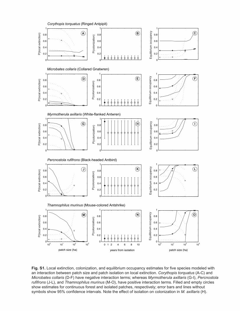
Species are fit by a variety of models, revealing a variety of possible responses to landscape change. For example, among the twelve species that were best fit by models with interaction between the effects of area and isolation on local extinction, six have negative and six have positive terms. Among species that have any model with interaction ranking above wj = 0.1, nine have positive and 10 have negative terms. Thus
we find no evidence that a particular kind of interaction was consistent across species. This may simply indicate the overall unimportance of interactions or, alternatively, it may reflect variation among species in response to landscape change. Negative interactions would indicate species that do poorly in small isolated patches; whereas, positive interactions would indicate species that have a very dynamic use of space in the continuous forest – hence showing high rates of local extinction in small continuous forest patches (Figure S1). Our vulnerability metrics do incorporate this variety of responses, including interactions on local extinction and the effects of regrowth on colonization, because they are based on the best-fitting model for each species.
0
0.2
0.4
0.6
0.8
1Corythopis torquatus (Ringed Antpipit)
Microbates collaris (Collared Gnatwren)
P(lo
cal e
xtin
ctio
n)P
(loca
l ext
inct
ion)
P(c
olon
izat
ion)
P(c
olon
izat
ion)
Equ
ilibr
ium
occ
upan
cyE
quili
briu
m o
ccup
ancy
0
0.2
0.4
0.6
0.8
1
0
0.2
0.4
0.6
0.8
1
0
0.2
0.4
0.6
0.8
1
0
0.2
0.4
0.6
0.8
1
0
0.2
0.4
0.6
0.8
1
A B C
D E F
0
0.2
0.4
0.6
0.8
1Myrmotherula axillaris (White-flanked Antwren)
P(lo
cal e
xtin
ctio
n)P
(loca
l ext
inct
ion)
P(c
olon
izat
ion)
P(c
olon
izat
ion)
Equ
ilibr
ium
occ
upan
cyE
quili
briu
m o
ccup
ancy
0
0.2
0.4
0.6
0.8
1
0
0.2
0.4
0.6
0.8
1
0
0.2
0.4
0.6
0.8
1
0.2
0.4
0.6
0.8
1Percnostola rufifrons (Black-headed Antbird)
100 101 102 103
patch size (ha)
Thamnophilus murinus (Mouse-colored Antshrike)
0 1 2 4 6 8 10
years from isolation patch size (ha)
P(lo
cal e
xtin
ctio
n)
P(c
olon
izat
ion)
Equ
ilibr
ium
occ
upan
cy
0
0.2
0.4
0.6
0.8
1
0
0.2
0.4
0.6
0.8
1
0
0.2
0.4
0.6
0.8
1
0
0.2
0.4
0.6
0.8
1
100 101 102 103
G H I
J K L
M N O
Fig. S1. Local extinction, colonization, and equilibrium occupancy estimates for five species modeled withan interaction between patch size and patch isolation on local extinction. Corythopis torquatus (A-C) and Microbates collaris (D-F) have negative interaction terms; whereas Myrmotherula axillaris (G-I), Percnostolarufifrons (J-L), and Thamnophilus murinus (M-O), have positive interaction terms. Filled and empty circles show estimates for continuous forest and isolated patches, respectively; error bars and lines without symbols show 95% confidence intervals. Note the effect of isolation on colonization in M. axillaris (H).
Table S1. The Excel file ‘Data.xls’ shows the data used in this study. The first worksheet explains the data file in detail; worksheets 2 to 56 show one data table per species. The last worksheet shows the sampling effort and the timing of patch isolation. Each row on a data table corresponds to one BDFFP study patch with the location name on the left and the size class in ha; numbered columns show sampling years. Ones and zeros represent visits to the site, with ‘1’ standing for detection of the species and ‘0’ for no detection. A dash means no visits for that site-year combination. For example, in 1984, the Dimona 100ha patch was visited four times but the species Automolus infuscatus was only detected there on the third visit; in 1989 there were no visits to that patch. Shaded areas show samples under isolation whereas clear areas correspond to continuous-forest samples. The number of visits per site per year stays constant across species, only the detections change. All the visits shown took place between the months of January and June.

Table S2. Diagram of model structures.The filled circles on the left indicate covariatesused to model colonization ( ) and local extinction ( ) within each model. Isolation andYear 1 are binary variables; Year 1 accounts for a possible increase in colonizationimmediately after the onset of isolation. Regrowth is 0 up to and including the year ofisolation; it starts counting at 1 the first year after isolation. Late Regrowth counts theyears of regrowth for models with an effect of Year 1 , starting at 2 the second year afterisolation. Models 1-5 consider only the effect of patch Size on local extinction; models6-10 consider an additive effect of Size and Isolation ; finally, models 11-15 consider aninteraction of Size and Isolation on local extinction. Initial occupancy ( 1) is always afree parameter and probability of detection (p) is assumed to vary with sampling effortalone.
EFFECTS
ColonizationLocal
extinction
Isol
atio
n
Yea
r1
Reg
row
th
Late
Reg
row
th
Siz
e
Isol
atio
n
Siz
eIs
ola
tion
MODEL NUMBER AND NAME
1. { 1(.), (.), (size),p(effort)}
2. { 1(.), (isol), (size),p(effort)}
3. { 1(.), (isol+year1), (size),p(effort)}
4. { 1(.), (isol+regrowth), (size),p(effort)}
5. { 1(.), (isol+year1+late regrowth), (size),p(effort)}
6. { 1(.), (.), (size+isol),p(effort)}
7. { 1(.), (isol), (size+isol),p(effort)}
8. { 1(.), (isol+year1), (size+isol),p(effort)}
9. { 1(.), (isol+regrowth), (size+isol),p(effort)}
10. { 1(.), (isol+year1+late regrowth), (size+isol),p(effort)}
11. { 1(.), (.), (size isol),p(effort)}
12. { 1(.), (isol), (size isol),p(effort)}
13. { 1(.), (isol+year1), (size isol),p(effort)}
14. { 1(.), (isol+regrowth), (size isol),p(effort)}
15. { 1(.), (isol+year1+late regrowth), (size isol),p(effort)}
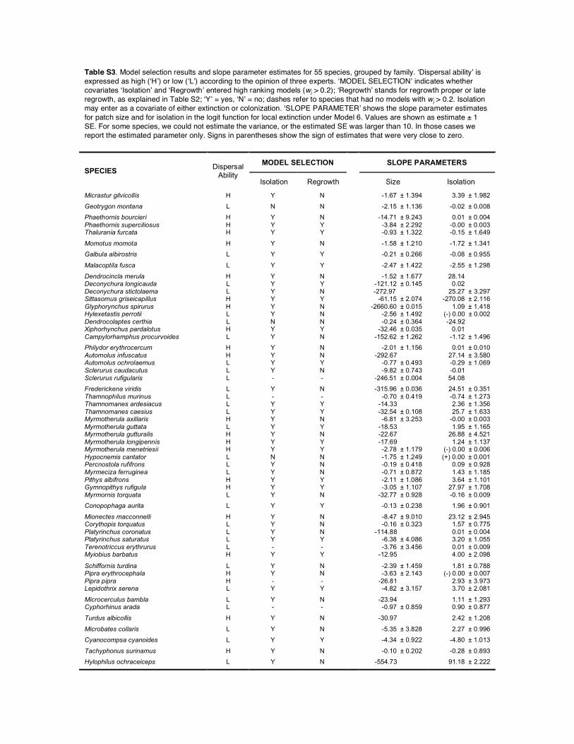
Table S3. Model selection results and slope parameter estimates for 55 species, grouped by family. ‘Dispersal ability’ is expressed as high (‘H’) or low (‘L’) according to the opinion of three experts. ‘MODEL SELECTION’ indicates whether covariates ‘Isolation’ and ‘Regrowth’ entered high ranking models (wj > 0.2); ‘Regrowth’ stands for regrowth proper or late regrowth, as explained in Table S2; ‘Y’ = yes, ‘N’ = no; dashes refer to species that had no models with wj > 0.2. Isolation may enter as a covariate of either extinction or colonization. ‘SLOPE PARAMETER’ shows the slope parameter estimates for patch size and for isolation in the logit function for local extinction under Model 6. Values are shown as estimate ± 1 SE. For some species, we could not estimate the variance, or the estimated SE was larger than 10. In those cases we report the estimated parameter only. Signs in parentheses show the sign of estimates that were very close to zero.
MODEL SELECTION
SLOPE PARAMETERS SPECIES Dispersal
Ability Isolation Regrowth Size Isolation
Micrastur gilvicollis H Y N -1.67 ± 1.394 3.39 ± 1.982 Geotrygon montana L N N -2.15 ± 1.136 -0.02 ± 0.008 Phaethornis bourcieri H Y N -14.71 ± 9.243 0.01 ± 0.004 Phaethornis superciliosus H Y Y -3.84 ± 2.292 -0.00 ± 0.003 Thalurania furcata H Y Y -0.93 ± 1.322 -0.15 ± 1.649 Momotus momota H Y N -1.58 ± 1.210 -1.72 ± 1.341 Galbula albirostris L Y Y -0.21 ± 0.266 -0.08 ± 0.955 Malacoptila fusca L Y Y -2.47 ± 1.422 -2.55 ± 1.298 Dendrocincla merula H Y N -1.52 ± 1.677 28.14 Deconychura longicauda L Y Y -121.12 ± 0.145 0.02 Deconychura stictolaema L Y N -272.97 25.27 ± 3.297 Sittasomus griseicapillus H Y Y -61.15 ± 2.074 -270.08 ± 2.116 Glyphorynchus spirurus H Y N -2660.60 ± 0.015 1.09 ± 1.418 Hylexetastis perrotii L Y N -2.56 ± 1.492 (-) 0.00 ± 0.002 Dendrocolaptes certhia L N N -0.24 ± 0.364 -24.92 Xiphorhynchus pardalotus H Y Y -32.46 ± 0.035 0.01 Campylorhamphus procurvoides L Y N -152.62 ± 1.262 -1.12 ± 1.496 Philydor erythrocercum H Y N -2.01 ± 1.156 0.01 ± 0.010 Automolus infuscatus H Y N -292.67 27.14 ± 3.580 Automolus ochrolaemus L Y Y -0.77 ± 0.493 -0.29 ± 1.069 Sclerurus caudacutus L Y N -9.82 ± 0.743 -0.01 Sclerurus rufigularis L - - -246.51 ± 0.004 54.08 Frederickena viridis L Y N -315.96 ± 0.036 24.51 ± 0.351 Thamnophilus murinus L - - -0.70 ± 0.419 -0.74 ± 1.273 Thamnomanes ardesiacus L Y Y -14.33 2.36 ± 1.356 Thamnomanes caesius L Y Y -32.54 ± 0.108 25.7 ± 1.633 Myrmotherula axillaris H Y N -6.81 ± 3.253 -0.00 ± 0.003 Myrmotherula guttata L Y Y -18.53 1.95 ± 1.165 Myrmotherula gutturalis H Y N -22.67 26.88 ± 4.521 Myrmotherula longipennis H Y Y -17.69 1.24 ± 1.137 Myrmotherula menetriesii H Y Y -2.78 ± 1.179 (-) 0.00 ± 0.006 Hypocnemis cantator L N N -1.75 ± 1.249 (+) 0.00 ± 0.001 Percnostola rufifrons L Y N -0.19 ± 0.418 0.09 ± 0.928 Myrmeciza ferruginea L Y N -0.71 ± 0.872 1.43 ± 1.185 Pithys albifrons H Y Y -2.11 ± 1.086 3.64 ± 1.101 Gymnopithys rufigula H Y Y -3.05 ± 1.107 27.97 ± 1.708 Myrmornis torquata L Y N -32.77 ± 0.928 -0.16 ± 0.009 Conopophaga aurita L Y Y -0.13 ± 0.238 1.96 ± 0.901 Mionectes macconnelli H Y N -8.47 ± 9.010 23.12 ± 2.945 Corythopis torquatus L Y N -0.16 ± 0.323 1.57 ± 0.775 Platyrinchus coronatus L Y N -114.88 0.01 ± 0.004 Platyrinchus saturatus L Y Y -6.38 ± 4.086 3.20 ± 1.055 Terenotriccus erythrurus L - - -3.76 ± 3.456 0.01 ± 0.009 Myiobius barbatus H Y Y -12.95 4.00 ± 2.098 Schiffornis turdina L Y N -2.39 ± 1.459 1.81 ± 0.788 Pipra erythrocephala H Y N -3.63 ± 2.143 (-) 0.00 ± 0.007 Pipra pipra H - - -26.81 2.93 ± 3.973 Lepidothrix serena L Y Y -4.82 ± 3.157 3.70 ± 2.081 Microcerculus bambla L Y N -23.94 1.11 ± 1.293 Cyphorhinus arada L - - -0.97 ± 0.859 0.90 ± 0.877 Turdus albicollis H Y N -30.97 2.42 ± 1.208 Microbates collaris L Y N -5.35 ± 3.828 2.27 ± 0.996 Cyanocompsa cyanoides L Y Y -4.34 ± 0.922 -4.80 ± 1.013 Tachyphonus surinamus H Y N -0.10 ± 0.202 -0.28 ± 0.893 Hylophilus ochraceiceps L Y N -554.73 91.18 ± 2.222
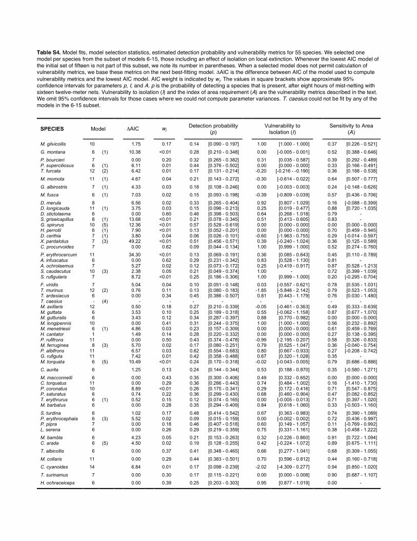
Table S4. Model fits, model selection statistics, estimated detection probability and vulnerability metrics for 55 species. We selected one model per species from the subset of models 6-15, those including an effect of isolation on local extinction. Whenever the lowest AIC model of the initial set of fifteen is not part of this subset, we note its number in parentheses. When a selected model does not permit calculation of vulnerability metrics, we base these metrics on the next best-fitting model. ΔAIC is the difference between AIC of the model used to compute vulnerability metrics and the lowest AIC model. AIC weight is indicated by wj. The values in square brackets show approximate 95% confidence intervals for parameters p, I, and A. p is the probability of detecting a species that is present, after eight hours of mist-netting with sixteen twelve-meter nets. Vulnerability to isolation (I) and the index of area requirement (A) are the vulnerability metrics described in the text. We omit 95% confidence intervals for those cases where we could not compute parameter variances. T. caesius could not be fit by any of the models in the 6-15 subset.
SPECIES Model
ΔAIC wj Detection probability (p)
Vulnerability to
Isolation (I)
Sensitivity to Area
(A)
M. gilvicollis 10 1.75 0.17 0.14 [0.090 - 0.197] 1.00 [1.000 - 1.000] 0.37 [0.226 - 0.521] G. montana 6 (1) 10.38 <0.01 0.28 [0.210 - 0.348] 0.00 [-0.005 - 0.001] 0.52 [0.388 - 0.646] P. bourcieri 7 0.00 0.20 0.32 [0.265 - 0.382] 0.31 [0.035 - 0.587] 0.39 [0.292 - 0.489] P. superciliosus 6 (1) 6.11 0.01 0.44 [0.376 - 0.502] 0.00 [0.000 - 0.000] 0.33 [0.166 - 0.491] T. furcata 12 (2) 6.42 0.01 0.17 [0.131 - 0.214] -0.20 [-0.216 - -0.190] 0.36 [0.188 - 0.538] M. momota 11 (1) 4.67 0.04 0.21 [0.143 - 0.272] -0.30 [-0.614 - 0.022] 0.64 [0.507 - 0.777] G. albirostris 7 (1) 4.33 0.03 0.18 [0.108 - 0.246] 0.00 [-0.003 - 0.003] 0.24 [-0.148 - 0.626] M. fusca 6 (1) 7.03 0.02 0.15 [0.093 - 0.198] -0.39 [-0.809 - 0.039] 0.57 [0.436 - 0.706] D. merula 8 6.56 0.02 0.33 [0.265 - 0.404] 0.92 [0.807 - 1.029] 0.16 [-0.088 - 0.399] D. longicauda 11 (1) 3.75 0.03 0.15 [0.096 - 0.213] 0.25 [0.019 - 0.477] 0.88 [0.720 - 1.035] D. stictolaema 6 0.00 0.60 0.46 [0.398 - 0.503] 0.64 [0.268 - 1.018] 0.79 - S. griseicapillus 8 (1) 13.68 <0.01 0.21 [0.078 - 0.345] 0.51 [0.413 - 0.605] 0.83 - G. spirurus 10 (5) 12.36 <0.01 0.57 [0.528 - 0.619] 0.00 [0.000 - 0.000] 0.00 [0.000 - 0.000] H. perrotii 6 (1) 7.90 <0.01 0.13 [0.052 - 0.201] 0.00 [0.000 - 0.000] 0.70 [0.459 - 0.945] D. certhia 7 (1) 3.80 0.04 0.06 [0.026 - 0.101] -0.60 [-1.963 - 0.755] 0.29 [-0.014 - 0.597] X. pardalotus 7 (3) 49.22 <0.01 0.51 [0.456 - 0.571] 0.39 [-0.240 - 1.024] 0.36 [0.125 - 0.589] C. procurvoides 7 0.00 0.62 0.09 [0.044 - 0.134] 1.00 [0.999 - 1.000] 0.52 [0.274 - 0.760] P. erythrocercum 11 34.30 <0.01 0.13 [0.069 - 0.191] 0.36 [0.085 - 0.643] 0.45 [0.110 - 0.789] A. infuscatus 6 0.00 0.62 0.29 [0.231 - 0.342] 0.83 [0.528 - 1.130] 0.81 - A. ochrolaemus 7 5.27 0.02 0.12 [0.073 - 0.172] 0.25 [-0.419 - 0.917] 0.87 [0.528 - 1.213] S. caudacutus 10 (3) 2.38 0.05 0.21 [0.049 - 0.374] 1.00 - 0.72 [0.399 - 1.039] S. rufigularis 7 8.72 <0.01 0.25 [0.186 - 0.306] 1.00 [0.999 - 1.000] 0.20 [-0.295 - 0.704] F. viridis 7 5.04 0.04 0.10 [0.051 - 0.148] 0.03 [-0.557 - 0.621] 0.78 [0.535 - 1.031] T. murinus 12 (2) 0.76 0.11 0.13 [0.080 - 0.183] -1.85 [-5.846 - 2.142] 0.79 [0.523 - 1.053] T. ardesiacus 6 0.00 0.34 0.45 [0.386 - 0.507] 0.81 [0.443 - 1.179] 0.76 [0.030 - 1.480] T. caesius - (4) - - - - - - - - M. axillaris 12 0.50 0.18 0.27 [0.210 - 0.339] -0.05 [-0.461 - 0.363] 0.49 [0.333 - 0.639] M. guttata 6 3.53 0.10 0.25 [0.189 - 0.318] 0.55 [-0.062 - 1.158] 0.87 [0.677 - 1.070] M. gutturalis 6 3.43 0.12 0.34 [0.287 - 0.397] 0.88 [0.770 - 0.982] 0.00 [0.000 - 0.000] M. longipennis 10 0.00 0.41 0.31 [0.244 - 0.375] 1.00 [1.000 - 1.000] 0.56 [0.232 - 0.892] M. menetriesii 6 (1) 4.86 0.03 0.23 [0.157 - 0.309] 0.00 [0.000 - 0.000] 0.61 [0.459 - 0.769] H. cantator 1 1.49 0.14 0.28 [0.220 - 0.332] 0.00 [0.000 - 0.000] 0.27 [0.138 - 0.395] P. rufifrons 11 0.00 0.50 0.43 [0.374 - 0.478] -0.99 [-2.195 - 0.207] 0.58 [0.326 - 0.833] M. ferruginea 8 (3) 5.70 0.02 0.17 [0.080 - 0.251] 0.79 [0.525 - 1.047] 0.36 [-0.040 - 0.754] P. albifrons 11 6.57 0.03 0.62 [0.554 - 0.683] 0.80 [0.667 - 0.933] 0.27 [-0.208 - 0.742] G. rufigula 11 7.42 0.01 0.42 [0.358 - 0.488] 0.67 [0.320 - 1.028] 0.35 - M. torquata 6 (5) 10.49 <0.01 0.24 [0.170 - 0.318] -0.02 [-0.043 - 0.005] 0.79 [0.686 - 0.886] C. aurita 6 1.25 0.13 0.24 [0.144 - 0.344] 0.53 [0.188 - 0.870] 0.35 [-0.580 - 1.271] M. macconnelli 6 0.00 0.43 0.35 [0.300 - 0.406] 0.49 [0.332 - 0.652] 0.00 [0.000 - 0.000] C. torquatus 11 0.00 0.29 0.36 [0.286 - 0.443] 0.74 [0.484 - 1.002] 0.16 [-1.410 - 1.730] P. coronatus 10 8.89 <0.01 0.26 [0.175 - 0.341] 0.29 [0.172 - 0.416] 0.71 [0.547 - 0.875] P. saturatus 6 0.74 0.22 0.36 [0.299 - 0.430] 0.68 [0.460 - 0.904] 0.47 [0.082 - 0.852] T. erythrurus 6 (1) 0.52 0.15 0.12 [0.074 - 0.165] 0.00 [-0.005 - 0.013] 0.71 [0.397 - 1.020] M. barbatus 6 0.00 0.28 0.35 [0.294 - 0.409] 0.84 [0.618 - 1.060] 0.33 [-0.503 - 1.160] S. turdina 6 1.02 0.17 0.48 [0.414 - 0.542] 0.67 [0.363 - 0.983] 0.74 [0.390 - 1.089] P. erythrocephala 6 (3) 5.52 0.02 0.09 [0.015 - 0.159] 0.00 [-0.002 - 0.002] 0.72 [0.436 - 0.997] P. pipra 7 0.00 0.18 0.46 [0.407 - 0.518] 0.60 [0.149 - 1.057] 0.11 [-0.769 - 0.992] L. serena 6 0.00 0.26 0.29 [0.219 - 0.359] 0.75 [0.331 - 1.161] 0.38 [-0.458 - 1.222] M. bambla 6 4.23 0.05 0.21 [0.153 - 0.263] 0.32 [-0.226 - 0.860] 0.91 [0.722 - 1.094] C. arada 6 (5) 4.50 0.02 0.19 [0.128 - 0.255] 0.42 [-0.224 - 1.072] 0.89 [0.675 - 1.111] T. albicollis 6 0.00 0.37 0.41 [0.348 - 0.465] 0.66 [0.277 - 1.041] 0.68 [0.309 - 1.055] M. collaris 11 0.00 0.29 0.44 [0.383 - 0.501] 0.70 [0.596 - 0.812] 0.44 [0.160 - 0.718] C. cyanoides 14 6.84 0.01 0.17 [0.098 - 0.239] -2.02 [-4.309 - 0.277] 0.94 [0.850 - 1.020] T. surinamus 7 0.00 0.30 0.17 [0.115 - 0.221] 0.00 [0.000 - 0.008] 0.90 [0.687 - 1.107] H. ochraceiceps 6 0.00 0.39 0.25 [0.203 - 0.303] 0.95 [0.877 - 1.019] 0.00 -
Supporting references and notes
S1. Bierregaard, Jr., R. O., T. E. Lovejoy, in Acta XIX Cong. Int. Ornith. H. Ouellet, Ed. (University of Ottawa Press, Ottawa, 1988), vol. II, pp. 1564-1579.
S2. G. Ferraz et al., Proc. Natl. Acad. Sci. U. S. A. 100, 14069 (2003). S3. J. A. Stratford, P. C. Stouffer, Conserv. Biol. 13, 1416 (1999). S4. P. C. Stouffer, R. O. Bierregaard, Jr., Ecology 76, 2429 (1995). S5. P. C. Stouffer, R. O. Bierregaard, Jr., Conserv. Biol. 9, 1085 (1995). S6. R. Alpizar-Jara et al., Oecologia 141, 652 (2004). S7. J. D. Nichols, T. Boulinier, J. E. Hines, K. H. Pollock, J. R. Sauer, Ecol. Appl. 8,
1213 (1998). S8. R. H. MacArthur, E. O. Wilson, The Theory of Island Biogeography (Princeton
University Press, Princeton, NJ, 1967). S9. I. Hanski, Metapopulation Ecology (Oxford University Press, Oxford, 1999). S10. M. Clinchy, D. T. Haydon, A. T. Smith, Am. Nat. 159, 351 (2002). S11. J. H. Brown, A. Kodric-Brown, Ecology 58, 445 (1977). S12. K. P. Burnham, D. R. Anderson, Model Selection and Multimodel Inference: A
Practical Information-Theoretic Approach (Springer, New York, 2002). S13. B. K. Williams, J. D. Nichols, M. J. Conroy, Analysis and Management of Animal
Populations (Academic Press, San Diego, 2002). S14. J. E. Hines. PRESENCE 2.0 (USGS-PWRC, 2004). S15. I. Hanski, Metapopulation Ecology (Oxford University Press, Oxford, 1999).