Reporting a one way repeated measures anova
45
Reporting a One-Way Repeated Measures ANOVA
-
Upload
ken-plummer -
Category
Education
-
view
3.088 -
download
2
Transcript of Reporting a one way repeated measures anova

Reporting a One-Way Repeated Measures ANOVA

Reporting the Study using APA
• Note – that the reporting format shown in this learning module is for APA. For other formats consult specific format guides.
• It is also recommended to consult the latest APA manual to compare what is described in this learning module with the most updated formats for APA

Reporting the Study using APA
• You can report that you conducted a One-Way Repeated Measures ANOVA by using the template below.

Reporting the Study using APA
• You can report that you conducted a One-Way Repeated Measures ANOVA by using the template below.
• “A one-way repeated measures ANOVA was conducted to compare the effect of (IV)______________ on (DV)_______________ in _________________, __________________, and __________________ conditions.”
• “A one-way repeated measures ANOVA was conducted to compare the effect of (IV) time of eating on (DV) pizza slices consumed, before, during and after the season.”
Reporting Results using APA

Reporting Results using APA
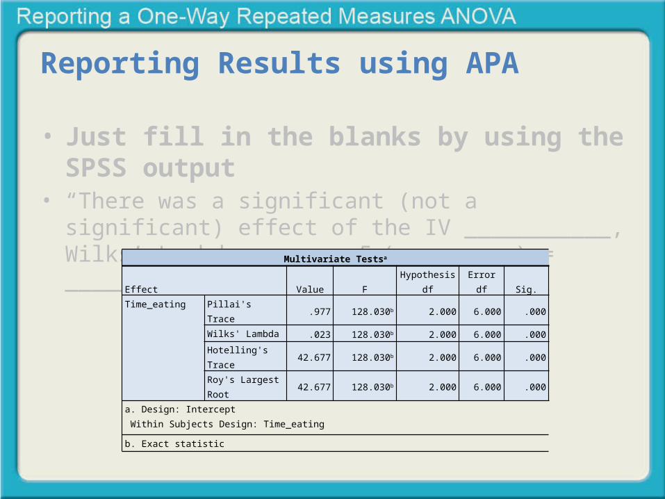
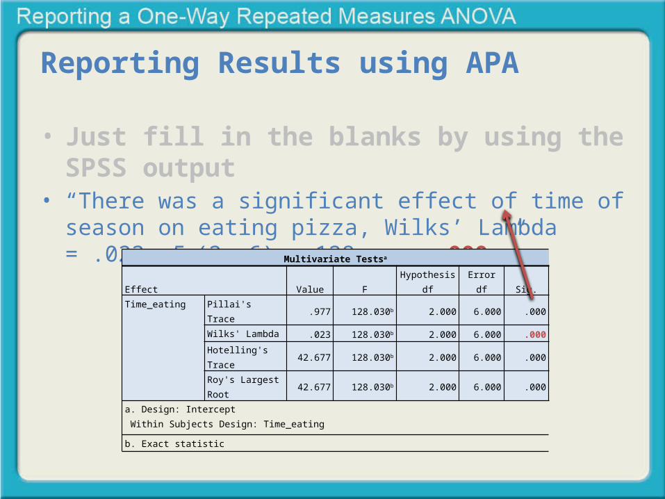
• Just fill in the blanks by using the SPSS output

Reporting Results using APA
• Just fill in the blanks by using the SPSS output• “There was a significant (not a significant) effect of the IV
___________, Wilks’ Lambda = ____, F (____,____) = _____, p = _____.
Reporting Results using APA
• Just fill in the blanks by using the SPSS output• “There was a significant (not a significant) effect of the IV
___________, Wilks’ Lambda = ____, F (____,____) = _____, p = _____.
Multivariate Testsa
Effect Value F Hypothesis df Error df Sig.
Time_eating Pillai's Trace .977 128.030b 2.000 6.000 .000
Wilks' Lambda .023 128.030b 2.000 6.000 .000
Hotelling's Trace 42.677 128.030b 2.000 6.000 .000
Roy's Largest Root 42.677 128.030b 2.000 6.000 .000
a. Design: Intercept
Within Subjects Design: Time_eating
b. Exact statistic

Reporting Results using APA
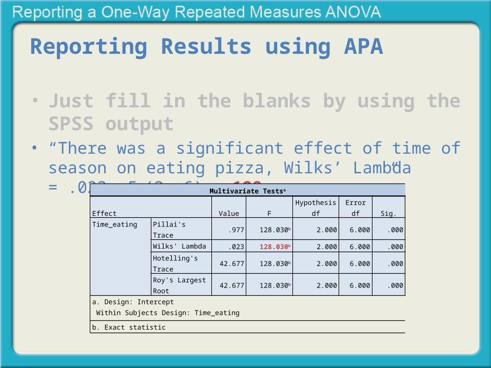
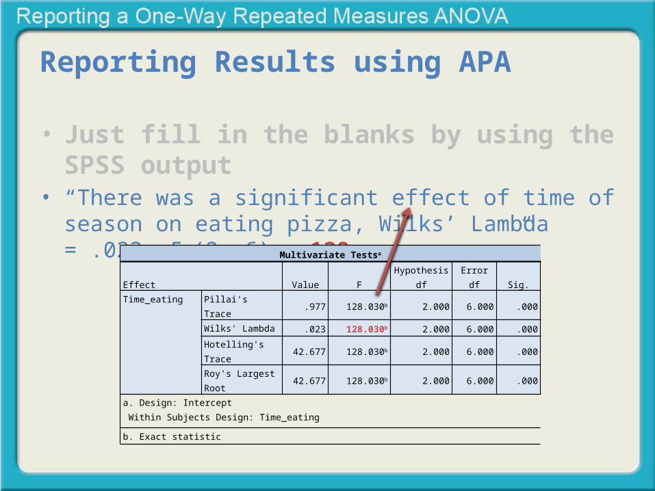
• Just fill in the blanks by using the SPSS output• “There was a significant effect of time of season on eating
pizza, Wilks’ Lambda = .023, F (____,____) = _____, p = _____.”
Multivariate Testsa
Effect Value F Hypothesis df Error df Sig.
Time_eating Pillai's Trace .977 128.030b 2.000 6.000 .000
Wilks' Lambda .023 128.030b 2.000 6.000 .000
Hotelling's Trace 42.677 128.030b 2.000 6.000 .000
Roy's Largest Root 42.677 128.030b 2.000 6.000 .000
a. Design: Intercept
Within Subjects Design: Time_eating
b. Exact statistic

Reporting Results using APA
• Just fill in the blanks by using the SPSS output• “There was a significant effect of time of season on eating
pizza, Wilks’ Lambda = .023, F (2,____) = _____, p = _____.”
Multivariate Testsa
Effect Value F Hypothesis df Error df Sig.
Time_eating Pillai's Trace .977 128.030b 2.000 6.000 .000
Wilks' Lambda .023 128.030b 2.000 6.000 .000
Hotelling's Trace 42.677 128.030b 2.000 6.000 .000
Roy's Largest Root 42.677 128.030b 2.000 6.000 .000
a. Design: Intercept
Within Subjects Design: Time_eating
b. Exact statistic

Reporting Results using APA
• Just fill in the blanks by using the SPSS output• “There was a significant effect of time of season on eating
pizza, Wilks’ Lambda = .023, F (2, 6) = _____, p = _____.”
Multivariate Testsa
Effect Value F Hypothesis df Error df Sig.
Time_eating Pillai's Trace .977 128.030b 2.000 6.000 .000
Wilks' Lambda .023 128.030b 2.000 6.000 .000
Hotelling's Trace 42.677 128.030b 2.000 6.000 .000
Roy's Largest Root 42.677 128.030b 2.000 6.000 .000
a. Design: Intercept
Within Subjects Design: Time_eating
b. Exact statistic
Reporting Results using APA
• Just fill in the blanks by using the SPSS output• “There was a significant effect of time of season on eating
pizza, Wilks’ Lambda = .023, F (2, 6) = 128, p = _____.”
Multivariate Testsa
Effect Value F Hypothesis df Error df Sig.
Time_eating Pillai's Trace .977 128.030b 2.000 6.000 .000
Wilks' Lambda .023 128.030b 2.000 6.000 .000
Hotelling's Trace 42.677 128.030b 2.000 6.000 .000
Roy's Largest Root 42.677 128.030b 2.000 6.000 .000
a. Design: Intercept
Within Subjects Design: Time_eating
b. Exact statistic
Reporting Results using APA
• Just fill in the blanks by using the SPSS output• “There was a significant effect of time of season on eating
pizza, Wilks’ Lambda = .023, F (2, 6) = 128, p = .000.”
Multivariate Testsa
Effect Value F Hypothesis df Error df Sig.
Time_eating Pillai's Trace .977 128.030b 2.000 6.000 .000
Wilks' Lambda .023 128.030b 2.000 6.000 .000
Hotelling's Trace 42.677 128.030b 2.000 6.000 .000
Roy's Largest Root 42.677 128.030b 2.000 6.000 .000
a. Design: Intercept
Within Subjects Design: Time_eating
b. Exact statistic

Reporting Results using APA
• Just fill in the blanks by using the SPSS output• “There was a significant effect of time of season on eating
pizza, Wilks’ Lambda = .023, F (2, 6) = 128, p = .000.”
• Once the blanks are full…you have your report:
Multivariate Testsa
Effect Value F Hypothesis df Error df Sig.
Time_eating Pillai's Trace .977 128.030b 2.000 6.000 .000
Wilks' Lambda .023 128.030b 2.000 6.000 .000
Hotelling's Trace 42.677 128.030b 2.000 6.000 .000
Roy's Largest Root 42.677 128.030b 2.000 6.000 .000
a. Design: Intercept
Within Subjects Design: Time_eating
b. Exact statistic

Reporting Results using APA
There was a significant effect of time of season on eating pizza, Wilks’ Lambda = .023, F (2, 6) = 128, p = .000.
Reporting Results using APA• Note- if there is a significant difference (which there was in
this case) you would also report the pair-wise t results which look like this:

Reporting Results using APA• Note- if there is a significant difference (which there was in
this case) you would also report the pair-wise t results which look like this:
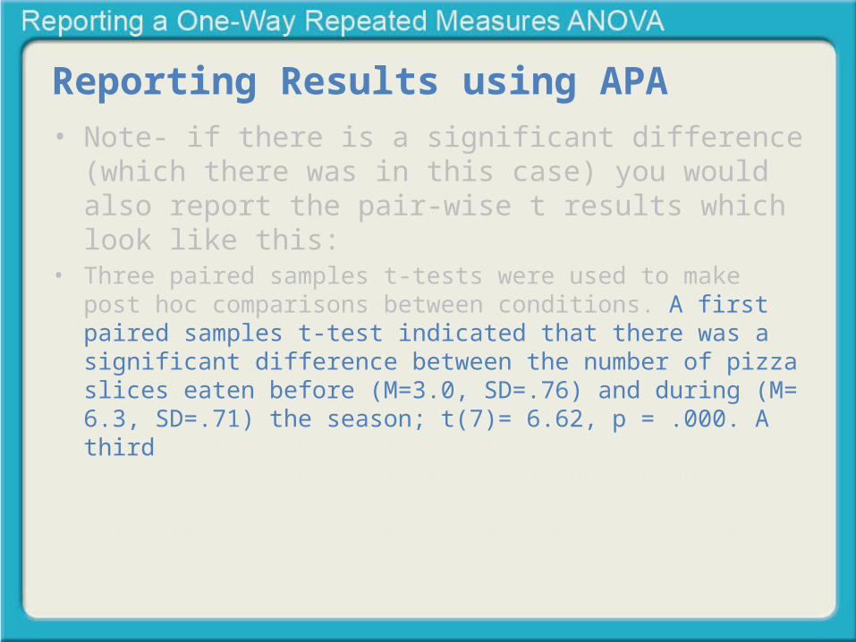
• Three paired samples t-tests were used to make post hoc comparisons between conditions.
Reporting Results using APA• Note- if there is a significant difference (which there was in
this case) you would also report the pair-wise t results which look like this:
• Three paired samples t-tests were used to make post hoc comparisons between conditions. A first paired samples t-test indicated that there was a significant difference between the number of pizza slices eaten before (M=3.0, SD=.76) and during (M= 6.3, SD=.71) the season; t(7)= 6.62, p = .000. A third paired samples t-test indicated that there was a significant difference between the number of pizza slices eaten before (M=3.0, SD=.76) and after (M =1.4, SD=.518) the season; t(7)= 6.18, p = .000.

Reporting Results using APA• Note- if there is a significant difference (which there was in
this case) you would also report the pair-wise t results which look like this:
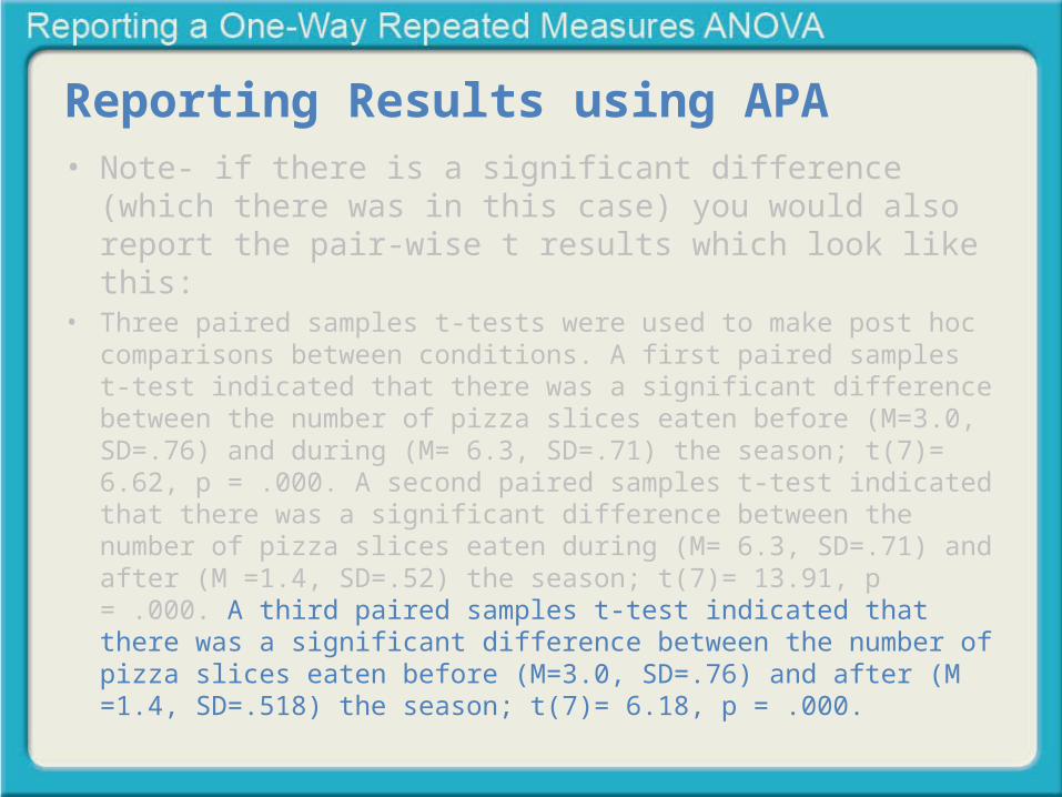
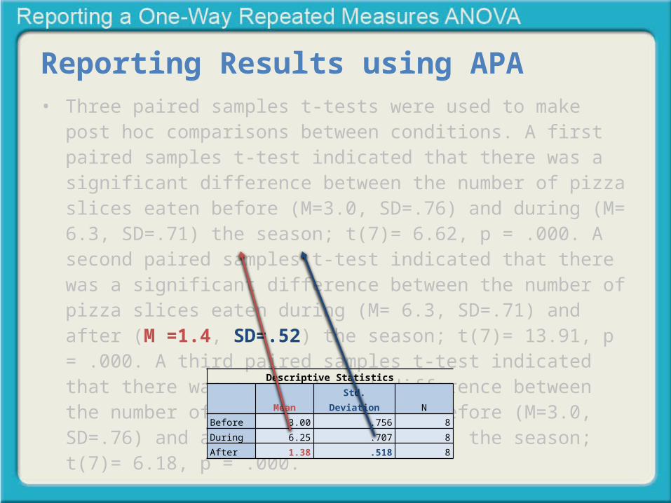
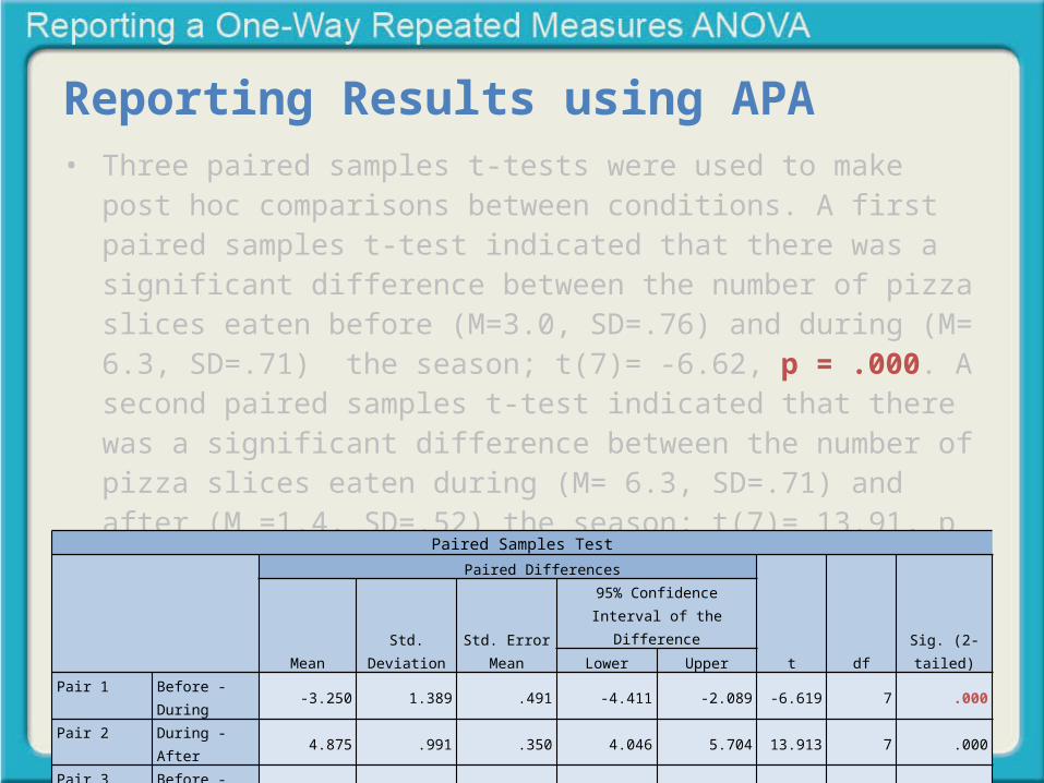
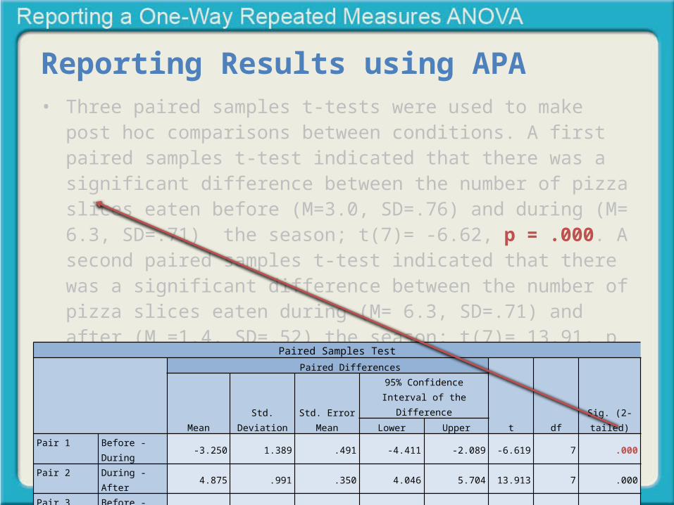
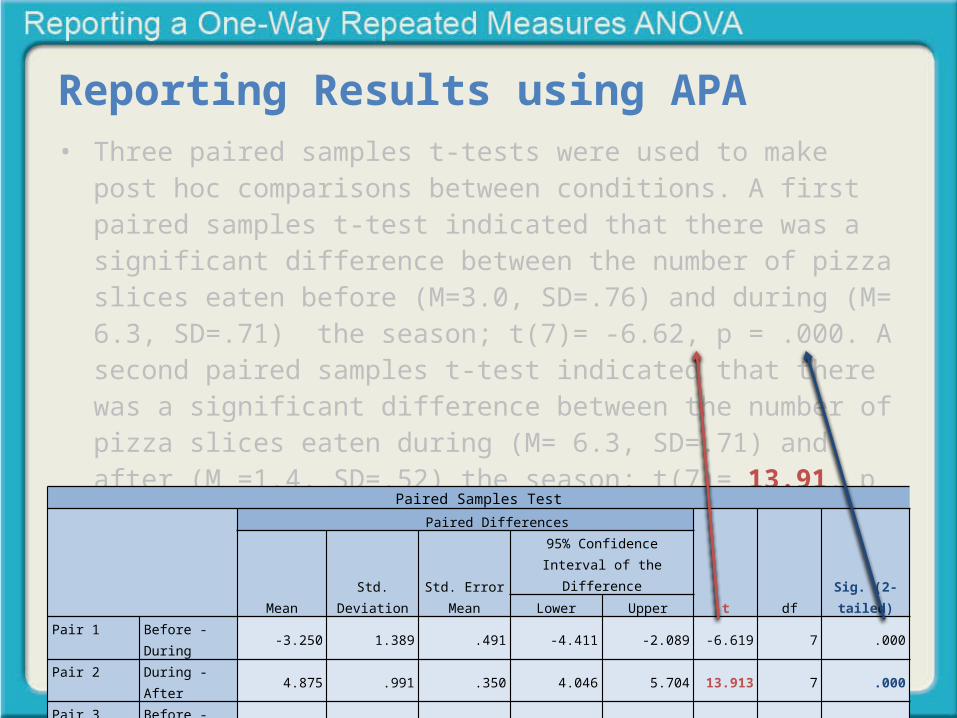
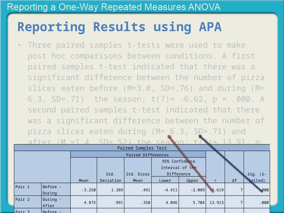
• Three paired samples t-tests were used to make post hoc comparisons between conditions. A first paired samples t-test indicated that there was a significant difference between the number of pizza slices eaten before (M=3.0, SD=.76) and during (M= 6.3, SD=.71) the season; t(7)= 6.62, p = .000. A second paired samples t-test indicated that there was a significant difference between the number of pizza slices eaten during (M= 6.3, SD=.71) and after (M =1.4, SD=.52) the season; t(7)= 13.91, p = .000. A third paired samples t-test indicated that there was a significant difference between the number of pizza slices eaten before (M=3.0, SD=.76) and after (M =1.4, SD=.518) the season; t(7)= 6.18, p = .000.
Reporting Results using APA• Note- if there is a significant difference (which there was in
this case) you would also report the pair-wise t results which look like this:
• Three paired samples t-tests were used to make post hoc comparisons between conditions. A first paired samples t-test indicated that there was a significant difference between the number of pizza slices eaten before (M=3.0, SD=.76) and during (M= 6.3, SD=.71) the season; t(7)= 6.62, p = .000. A second paired samples t-test indicated that there was a significant difference between the number of pizza slices eaten during (M= 6.3, SD=.71) and after (M =1.4, SD=.52) the season; t(7)= 13.91, p = .000. A third paired samples t-test indicated that there was a significant difference between the number of pizza slices eaten before (M=3.0, SD=.76) and after (M =1.4, SD=.518) the season; t(7)= 6.18, p = .000.

Reporting Results using APA• Three paired samples t-tests were used to make post hoc comparisons
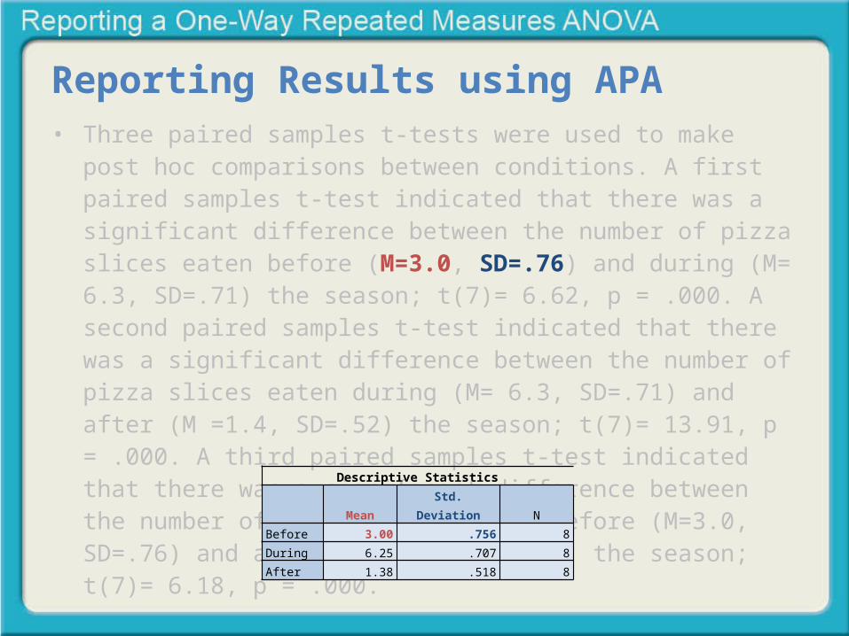
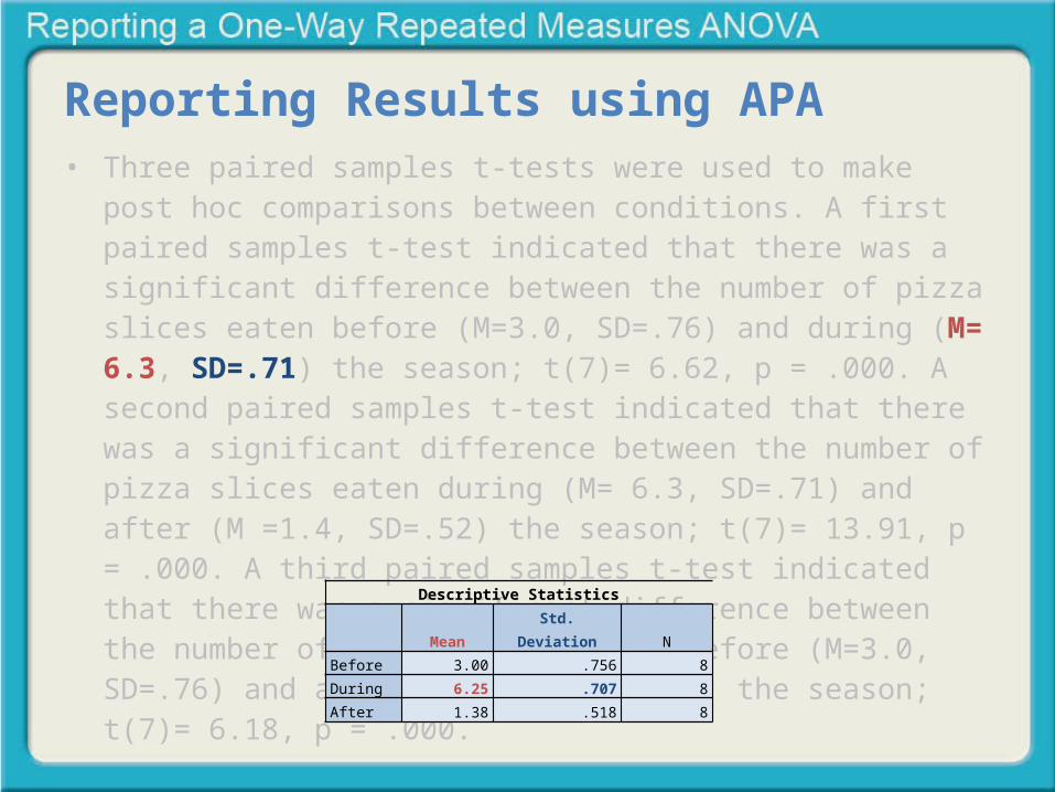
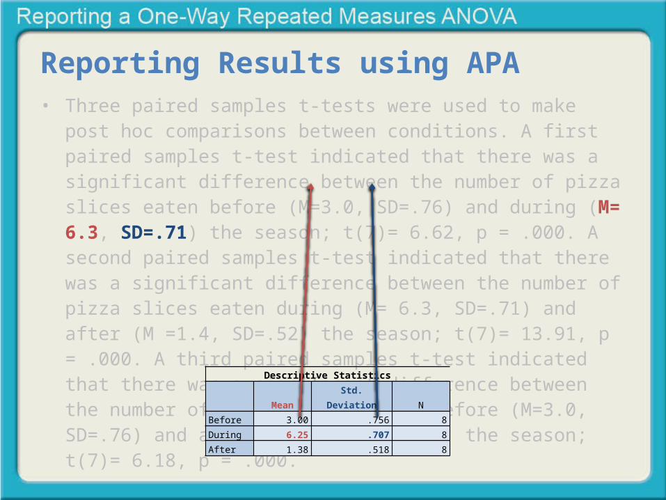
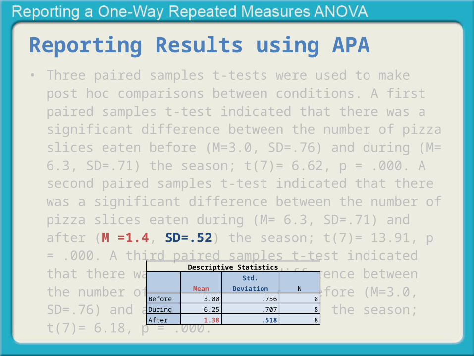
between conditions. A first paired samples t-test indicated that there was a significant difference between the number of pizza slices eaten before (M=3.0, SD=.76) and during (M= 6.3, SD=.71) the season; t(7)= 6.62, p = .000. A second paired samples t-test indicated that there was a significant difference between the number of pizza slices eaten during (M= 6.3, SD=.71) and after (M =1.4, SD=.52) the season; t(7)= 13.91, p = .000. A third paired samples t-test indicated that there was a significant difference between the number of pizza slices eaten before (M=3.0, SD=.76) and after (M =1.4, SD=.518) the season; t(7)= 6.18, p = .000.
Descriptive Statistics
Mean Std. Deviation N
Before 3.00 .756 8
During 6.25 .707 8
After 1.38 .518 8
Reporting Results using APA• Three paired samples t-tests were used to make post hoc comparisons
between conditions. A first paired samples t-test indicated that there was a significant difference between the number of pizza slices eaten before (M=3.0, SD=.76) and during (M= 6.3, SD=.71) the season; t(7)= 6.62, p = .000. A second paired samples t-test indicated that there was a significant difference between the number of pizza slices eaten during (M= 6.3, SD=.71) and after (M =1.4, SD=.52) the season; t(7)= 13.91, p = .000. A third paired samples t-test indicated that there was a significant difference between the number of pizza slices eaten before (M=3.0, SD=.76) and after (M =1.4, SD=.518) the season; t(7)= 6.18, p = .000.
Descriptive Statistics Mean Std. Deviation N
Before 3.00 .756 8
During 6.25 .707 8
After 1.38 .518 8

Reporting Results using APA• Three paired samples t-tests were used to make post hoc comparisons
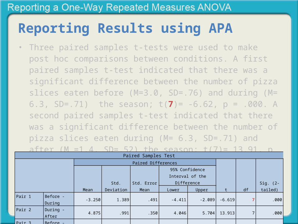
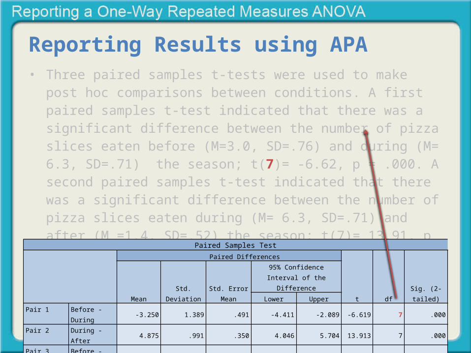
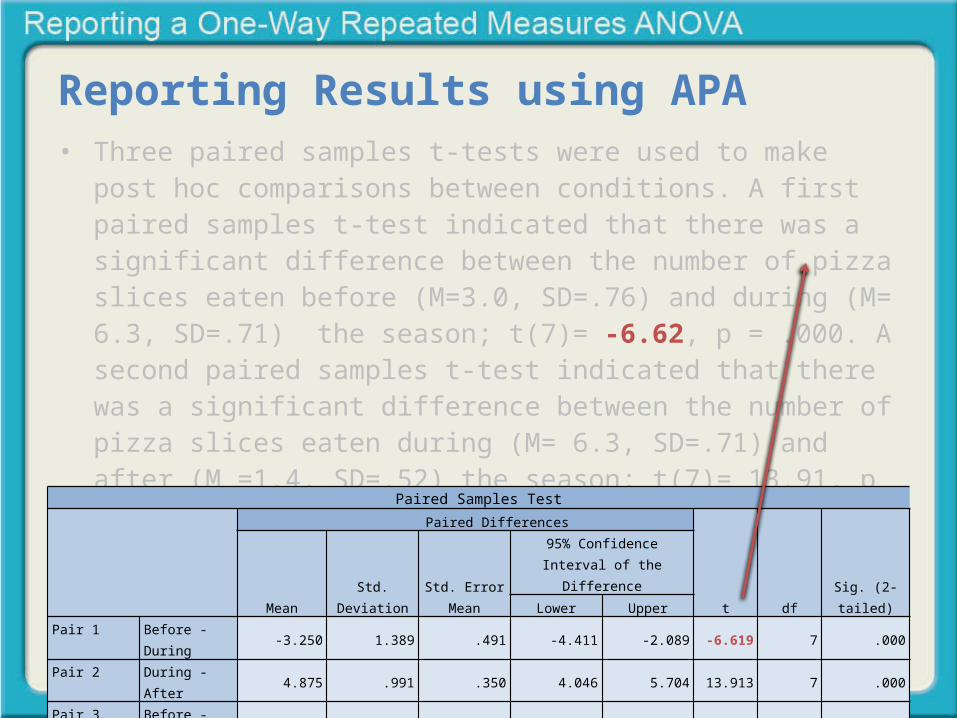
between conditions. A first paired samples t-test indicated that there was a significant difference between the number of pizza slices eaten before (M=3.0, SD=.76) and during (M= 6.3, SD=.71) the season; t(7)= -6.62, p = .000. A second paired samples t-test indicated that there was a significant difference between the number of pizza slices eaten during (M= 6.3, SD=.71) and after (M =1.4, SD=.52) the season; t(7)= 13.91, p = .000. A third paired samples t-test indicated that there was a significant difference between the number of pizza slices eaten before (M=3.0, SD=.76) and after (M =1.4, SD=.518) the season; t(7)= 6.18, p = .000.
Paired Samples Test
Paired Differences
t df Sig. (2-tailed)Mean Std. Deviation
Std. Error
Mean
95% Confidence Interval of the
Difference
Lower Upper
Pair 1 Before - During -3.250 1.389 .491 -4.411 -2.089 -6.619 7 .000
Pair 2 During - After 4.875 .991 .350 4.046 5.704 13.913 7 .000
Pair 3 Before - After 1.625 .744 .263 1.003 2.247 6.177 7 .000
Reporting Results using APA• Three paired samples t-tests were used to make post hoc comparisons
between conditions. A first paired samples t-test indicated that there was a significant difference between the number of pizza slices eaten before (M=3.0, SD=.76) and during (M= 6.3, SD=.71) the season; t(7)= -6.62, p = .000. A second paired samples t-test indicated that there was a significant difference between the number of pizza slices eaten during (M= 6.3, SD=.71) and after (M =1.4, SD=.52) the season; t(7)= 13.91, p = .000. A third paired samples t-test indicated that there was a significant difference between the number of pizza slices eaten before (M=3.0, SD=.76) and after (M =1.4, SD=.518) the season; t(7)= 6.18, p = .000.
Paired Samples Test
Paired Differences
t df Sig. (2-tailed)Mean Std. Deviation
Std. Error
Mean
95% Confidence Interval of the
Difference
Lower Upper
Pair 1 Before - During -3.250 1.389 .491 -4.411 -2.089 -6.619 7 .000
Pair 2 During - After 4.875 .991 .350 4.046 5.704 13.913 7 .000
Pair 3 Before - After 1.625 .744 .263 1.003 2.247 6.177 7 .000