Report on support to CEN TC89/WG8

Update of ISO 9869 to EN12494 "in-situ measurement of the thermal resistance and thermal transmittance"

by

PASLINK EEIG

edited (1995) by

J.J. BLOEM Joint Research Centre

Institute for Systems Engineering and Informatics I - 21020 Ispra, ITALY

Updated March 2002. Note that the information below refers to the tools available in 1995. At present, the PASLINK organisation has converted MRQT into a more user-friendly tool, named LORD. The program CTLSM is extended and is called now CTSM. Furthermore the PEM routine is now available as a routine IDENT in the System Identification Toolbox of the Matlab environment. In all cases reference is made to the tool information on the PASLINK web-site, section Data Analysis.

1. CONTENTS 2

2. INTRODUCTION 4

2.1 CEN TC89/WG8 4

2.2 PASLINK 4

2.3 PASLINK and CEN TC89/WG8 5 2.3.1 The CEN Performance Check 5 2.3.2 Chapter 10 and Annex A 6

3. WALL DESCRIPTION 7

3.1 Introduction 7

3.2 Data Series 7 3.2.1 Data compression 7 3.2.2 Four performance tests 7 3.2.3 Access to the data 9

4. FOURIER COEFFICIENT TABLES 10

4.1 Theory of compression 10

4.2 Compression in 38 frequencies 11

4.3 Accuracy of compression 11

4.4 Theory of the heat flux through a wall 12

4.5 Simulation of the heat flux in general 12

4.6 Heat flux simulation for compressed temperatures 13

4.7 Conclusion 14

5. APPLICATION USING DIFFERENT METHODS; PEM, CTLSM, MRQT 19

5.1 Introduction 19 5.1.1 Creation of different testsets 19 5.1.2 Tests on different test sets 20

5.2 PEM applied 22 5.2.1 Generation of data 22 5.2.2 Model 22 5.2.3 Test method 23 5.2.4 Results of tests 24 5.2.5 Conclusions 25 5.2.6 Discussion and remarks on Annex A of the CEN-standard 25

5.3 CTLSM applied 26 5.3.1 Introduction 26 5.3.2 The chosen model 26 5.3.3 Calculated statistics 26 5.3.4 Test of the confidence interval 26 5.3.5 Test 3 26 5.3.6 Conclusion 26

5.4 MRQT applied 27 5.4.1 Introduction 27 5.4.2 Dynamic model 27 5.4.3 Results 27 5.4.4 Discussion 27 5.4.5 Conclusion 27

6. A COMPARISON OF METHODS 28

6.1 Introduction 28

6.2 Methods 28 6.2.1 The one-dimensional heat equation 28 6.2.2 The average method. 29 6.2.3 Lumped parameter model. 29 6.2.4 A linear model. 29 6.2.5 A state-space model. 30 6.2.6 A frequency model. 30

7. SYSTEM IDENTIFICATION COMPETITION 31

7.1 Objective 31

7.2 Introduction 31

7.3 Case Descriptions 32

7.4 Access to the data 33

8. CONCLUSIONS 33

9. FINAL DOCUMENT AS SUBMITTED FOR PREN 34

10. REFERENCES 35

1.

2. Introduction

The EC is searching for standardized methodologies for the assessment of thermal parameters for different types of building components. Dynamic system identification techniques are the most promising methods to achieve this goal. Development of assessment procedures and guidelines is one of the objectives of the EC. Within the frame of the DGXII PASSYS project the work by the participating teams has been concentrated on the development of reliable parameter identification methods. Methods developed in the subgroup Test Methodologies of the PASSYS project are based on a lumped parameter model and a continuous time model, modal models and armax models. The application of identification methods on "in-situ measurement of the thermal resistance and thermal transmittance" will be discussed. A performance check for these methods will be presented, which includes tests on noise, change of input signal by uncontrolled phenomena and non linear parameter behaviour. The application of several methods will be discussed in referenced papers.

2.1 CEN TC89/WG8

CEN, Commitee Europeen de Normalisation, is organised through Technical Committees. The area of CEN/TC 89 is on Thermal Performance of Buildings and Building Components. Working Group 8 of the CEN/TC89 deals with Thermal Test Methods [5]. Its scope is to deal with standards on test methods for determining thermal properties of building materials, products and components, including the insulation of equipment. In the task is included consideration of accuracy levels appropriate to the subsequent treatment of results and guidleines to assess the apparatus and testing procedures used by laboratories.

2.2 PASLINK

The EC project PASSYS, started in 1986, has set-up a network of at present 14 high quality test sites equipped with test cells for the outdoor evaluation of thermal and solar performances of building components. A very important activity is the development of appropriate test methods for the identification of the thermal and solar characteristics of building components under real weather conditions. The most promising techniques for the assessment of the characteristics are dynamic analysis tools. Within the frame of pre-normative research a performance test has been developed aiming to offer for the CEN standard on "in-situ measurements of thermal resistance" a series of reliable dynamic analysis tools. Advantages of dynamic methods compared to the generally applied average method are illustrated in several papers which deal with real in-situ measurements on simple walls. The error analysis is an essential part of the work and is supported by several teams specialised in statistics. As a result of the work performed by the PASSYS subgroup on Test Methodologies a continuation under the PASLINK project was performed on the implementation of dynamic analysis tools for assessment of the thermal resistance from in-situ measurements.

2.3 PASLINK and CEN TC89/WG8

During 1992 contacts with the convenor of CEN TC89/WG8 led to a fruitful collaboration between several teams of PASLINK and WG8 [2, 3]. The aim was to modify the existing ISO 9869 document regarding three major issues. First the measurement accuracy (temperature and heat flux sensors) which is a crucial issue for the standard. Secondly the measurement disturbance like mass transfer will be considered. Thirdly the analysis of the data. In the existing ISO 9869 standard [1] the average method is the reference and one specific dynamic is described in the annex. No information on the accuracy is given and to modern standards the method is not very satisfying. Three objectives were defined:

• modify the existing ISO 9869 standard in terms of quality • introduce dynamic analysis tools by means of performance checks • demonstration of the application of the performance check

A general identification method that can be used in all cases does not exist. Rather a set of methods can be envisaged, where each method is more suitable than other methods in a particular situation. The methods differ with respect to their possibility to incorporate physical knowledge about the thermal system modelled, to use different types of data and their robustness with respect to measurement errors and other pitfalls. 2.3.1 The CEN Performance Check A wide range of new techniques is now being applied to the analysis problems involved in the assessment of thermal characteristics of buildings and building components. During the past the need for benchmark tests for dynamically analysis methods has been notified. It can be seen as a result of the work done in several European projects that an input is prepared for a CEN standard on the "in-situ measurement of the thermal resistance and thermal transmittance" (CEN TC89/WG8). The most important part of the modification of ISO 9869 deals with the dynamic method which seems to be difficult and has not been applied to a large extent. A series of performance tests have been developed and tested on several modern methods. Synthetic data for these tests have to be rebuilt from tables with Fourier coefficients which describe the input signals. The list with Fourier coefficients describe seasonal variation as well as daily variation of the in- and outdoor surface temperatures. The flux will be expressed by complex thermal resistance's to allow a more flexible system in varying the conditions. Data can be obtained also from the net-server at the JRC Ispra (see chapter 3.2.2). Three imaginary walls have been selected to test the methods on the extreme cases. Results of these exercises with MRQT, LADY, CTLSM and GLM have been reported. An overall agreement on the proposed performance check has been made which allows the participants to test their applied method on the performance check. Several papers show the superiority of dynamic analysis tools over the average method which results in a higher accuracy, shorter and therefore more reliable data series and dynamic information. Figure 1 illustrates this for simulated data applied on a lightweight wall component. Changes in the physical system or non constant parameters can be identified as well, for example by analyzing the residual data.

2.3.2 Chapter 10 and Annex A A short description of the performance check will be given here. It will appear in the CEN standard in chapter 10 (Analysis of data) and the normative Annex A (Assessment of the analysis method and related data sets). Four tests each for three walls, differing in thermal mass and heat resistance, are included in the performance check. The selected walls represent the extreme cases and are not necessarily realistic. Furthermore the check provides evaluation criteria for classification of methods. Synthetic data, but realistic as much as possible, have been created using the physical theory of heat transfer in a layer. To simulate the heat flux properly, the simulation model must be based on the theoretical derived differential equations. This equation can only be solved in the frequency domain, therefore fourier transformation has been applied. In the framework of the CEN standardisation it is required to have all information written on paper. Compression of data series of more than 8000 points has been performed by using Fourier analysis and selecting the 38 most important frequencies. Simple equations can be applied to re-built the data series from these tables of Fourier coefficients. Four tests have been designed in such a way that a classification of dynamic methods is possible. The data series are made for one year and contain seasonal variation as well as daily variation. It allows the user to perform cross validation of its model. The method should run 24 short periods throughout these data series. The duration of this period depends on the time constant of the wall and the method and should be mentioned as well. Results of the tests should be reported in a defined way which includes graphical presentation of the confidence interval. The following tests have been designed: Test 1 Clean data series, without noise, containing exact information Test 2 Gaussian noise is added to the signals; in- and outdoor temperatures and the heat flux. Test 3 A systematic error is introduced in one of the input signals. Test 4 Mass transfer in the wall is simulated. The method should detect the phenomena of a linear temperature dependent thermal resistance.

3. Wall description

3.1 Introduction

In the EC DG-XII Passys project several dynamic identification methods have been developed to determine the surface-to-surface thermal resistance of walls. These methods are different from the dynamical method described in the present ISO-standard. Since there exist a growing number of potentially powerful analysis methods it is not appropriate to impose one particular method. Performance checks are necessary to which a chosen analysis has to be objected. The CEN-standard under study for modification, will contain such a performance check. The performance check contains four tests each for three walls, differing in thermal mass and heat resistance. The check provides evaluation criteria for classification of methods [4]. This paper describes the results of the work done at the JRC in Ispra, concerning the creation of Fourier coefficient tables for the performance check. Note that for the standard, all information should be available in a written format. The data is however available in electronic format as well. On request (send an e-mail to hans.bloem@jrc.it ) the data can be made available.

3.2 Data Series

3.2.1 Data compression Synthetic data, but realistic as much as possible, have been created using TRY data for the outdoor temperature and the physical theory of heat transfer in a layer for the flux through the wall. To simulate the heat flux properly, the simulation model must be based on the theoretical derived differential equations. This equation can only be solved in the frequency domain, therefore a Fourier transform has been applied. Within the framework of a CEN standard it is not acceptable to produce time series each consisting of some 1000 or more individual data points, techniques have to be selected which make it possible to compress the high number of individual observations into a small number of parameters. However applying a compression method, some information of the signal will be lost. The type of compression that is applied uses Fourier series. Simple equations can be applied to re-built the dataseries from these tables of Fourier coefficients. Most important information of the original signal, the harmonic information, will be saved. 3.2.2 Four performance tests The dataseries are made for one year (8736 data points, based on hourly data) and contain seasonal variation as well as daily variation. It allows the user to perform cross validation of the aused model. The method should run 24 short periods throughout this dataserie. The duration of the periods are related to the time constant of the wall and the method and should be mentioned as well in the resulting output. Results of the tests should be reported in a defined way which includes graphical presentation of the confidence interval. Four tests have been designed in such a way that a classification of dynamical methods is possible. • Test 1 Clean data series, without noise, containing exact information • Test 2 Gaussian noise is added to the signals, In- and Outdoor temperature and

the heat flux. • Test 3 A systematic error is introduced in one of the input signals. • Test 4 Mass transfer in the wall is simulated. The method should detect this phenomena. The properties of the 3 walls as defined by CEN TC89/WG8 during discussions at several meetings, can be found in table 1. The selected walls represent the extreme cases and are not necessarily realistic which may be concluded from the table.

wall 1 layer material thickness

d [m] cond.

[W/m .K] density [kg/m3]

heat cap. [J/kg.K]

thermal resist.

[Km2/W]

heat cap. [J/K.m2]

1 facing 0.01 0.100 600 1000 0.10 6000 2 insulation 0.40 0.035 30 1000 11.42857 12000 3 facing 0.01 0.100 600 1000 0.10 6000 total thermal

resistance [Km2/W] total heat

capacitance [J/K.m2] time constant

[days] 11.62857 24000 3.23

wall 2 layer material thickness

d [m] cond.

[W/m .K] density [kg/m3]

heat cap. [J/kg.K]

thermal resist.

[Km2/W]

heat cap. [J/K.m2]

1 facing 0.01 0.100 600 1000 0.10 6000 2 insulation 0.05 0.035 30 1000 1.42857 1500 3 masonry 0.30 0.700 1800 1000 0.42857 540000 4 insulation 0.15 0.035 30 1000 4.28571 4500 5 facing 0.01 0.100 600 1000 0.10 6000 total thermal

resistance [K m2/W] total heat

capacitance [J/K.m2] timeconstant

[days] 6.34286 558000 41.01

wall 3 layer material thickness

d [m] cond.

[W/m .K] density [kg/m3]

heat cap. [J/kg.K]

thermal resist.

[Km2/W]

heat cap. [J/K.m2]

1 masonry 0.40 0.200 800 1000 2.00 320000 total thermal

resistance [K m2/W] total heat

capacitance [J/K.m2] timeconstant

[days] 2.00 320000 7.41

Table 1 shows the properties of the selected walls

Tables have been created containing 38 frequencies for the temperatures and fluxes. Temperatures and heat fluxes contain frequencies up to 3 hours. Please note that equation 1-3 (DC-signal) and the length of the dataset (in days) are specific for the corresponding tables. Temperatures can be generated form the coefficients found in table 2. In table 3a and b the coefficients for the fluxes of the different walls can be found in a new presentation as required by CEN TC89/WG8 in the proposal [4, 5]. Now it is possible to have the flux calculated in a

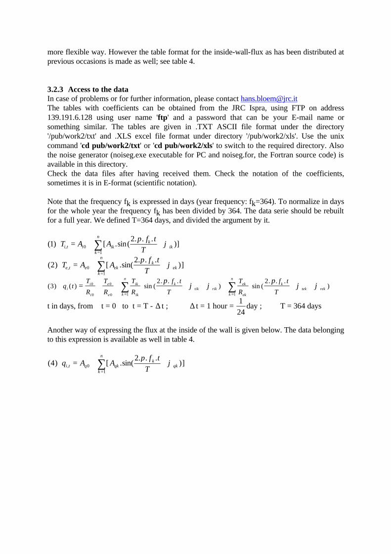
more flexible way. However the table format for the inside-wall-flux as has been distributed at previous occasions is made as well; see table 4. 3.2.3 Access to the data In case of problems or for further information, please contact hans.bloem@jrc.it The tables with coefficients can be obtained from the JRC Ispra, using FTP on address 139.191.6.128 using user name 'ftp' and a password that can be your E-mail name or something similar. The tables are given in .TXT ASCII file format under the directory '/pub/work2/txt' and .XLS excel file format under directory '/pub/work2/xls'. Use the unix command 'cd pub/work2/txt' or 'cd pub/work2/xls' to switch to the required directory. Also the noise generator (noiseg.exe executable for PC and noiseg.for, the Fortran source code) is available in this directory. Check the data files after having received them. Check the notation of the coefficients, sometimes it is in E-format (scientific notation). Note that the frequency fk is expressed in days (year frequency: fk=364). To normalize in days for the whole year the frequency fk has been divided by 364. The data serie should be rebuilt for a full year. We defined T=364 days, and divided the argument by it.

( ) [ .sin(. . .

)],12

01

T A Af t

Ti t i ikk

ikk

n

= + +=

∑ πϕ

( ) [ .sin(. . .

)],22

01

T A Af t

Te t e ekk

ekk

n

= + +=

∑ πϕ

( ) ( ) sin (. . .

) sin (. . .

)32 20

0

0

0 1 1

q tT

R

T

R

T

R

f t

T

T

R

f t

Ti

i

i

e

e

ik

ik

ktik rik

k

nek

ek

ktek rek

k

n

= + + ⋅ + + + ⋅ + += =

∑ ∑πϕ ϕ

πϕ ϕ

t in days, from t = 0 to t = T - ∆ t ; ∆ t = 1 hour = 1

24day ; T = 364 days

Another way of expressing the flux at the inside of the wall is given below. The data belonging to this expression is available as well in table 4.

( ) [ .sin(. . .

)],42

01

q A Af t

Ti t q qkk

qkk

n

= + +=

∑ πϕ

4. Fourier coefficient tables

This performance check requires synthetic data series (surface temperatures and heat flux) for walls with different thermal properties in order to check a dynamical method under different conditions. These data series have to be compressed because the CEN standard requires a distribution of the data on an A4 page [5]. In this chapter the theory of compression and the simulation of the heat flux is described. Computer programs to compress, to decompress and to simulate the heat flux have been developed in MATLAB [9] and can be found in [31].

4.1 Theory of compression

The French engineer Jean Baptiste Joseph Fourier [6] proved that any arbitrary function, even one with a finite number of discontinuities, could be represented as an infinite summation of sine and cosine terms. Compressing a data series by writing it as a sum of sine functions correspond with applying a discrete Fourier transform for a limited number of frequencies. To compress a data series to a small number of parameters, the main frequencies of the signal have to be determined and for a selected number of these main frequencies the data series can be compressed. In this case some information of the signal will be lost and the residue (i.e. the difference between the original data series and the decompressed from the fourier coefficients) contains the not selected frequencies. For the main frequencies the coefficients (Aik and jik) are calculated, and the data series can be written as a sum of sine functions;

T A Af t

Ti t i ikk

ikk

n

, [ .sin(. . .

)]= + +=

∑01

2 πϕ (1)

The DC-component of Ti,t is called Ai0 and has a zero-phase. The coefficients in equation (1) can be calculated by using the following derivation ;

f t c e c c e c eni n t

nn

i n tn

i n t

n

( ) = ⋅ = + ⋅ + ⋅ =⋅ ⋅ ⋅

=−∞

∞⋅ ⋅ ⋅

−− ⋅ ⋅ ⋅

=

∞

∑ ∑ω ω ω1 1 10

1

(2)

( )( ) ( )( )= + + ⋅ + ⋅ + − ⋅ − ⋅ ==

∞

∑c a i b n t i n t a i b n t i n tn n n nn

012 1 1

12 1 1

1

{ cos sin cos sinω ω ω ω (3)

( )= + + = + + ⋅ + ==

∞

=

∞

∑ ∑12 0 1 1

1

12 0

2 21

1

a a n t b n t a a b n tn nn

n nn

cos sin sinω ω ω ϕ

(4)

= + ⋅⋅ ⋅ ⋅

+=

∞

∑A Af t

Ti ikk

ikk

01

2sin( )

πϕ (5)

with c a i b

c a i bn n n

n n n

= + ⋅

= − ⋅−

12

12

( )

( ) and

a c c

b i c cn n

n n

= +

= − ⋅ −−

−

1

1( ) and ϕ =

arctan

a

bn

n

Because equation (2) is similar to a discrete Fourier transform, the fast Fourier transform can be used to calculate the coefficients.

4.2 Compression in 38 frequencies

It is required in a CEN-standard to distribute data series fitting on an A4 page, therefor a limited number of frequencies have to be selected. At the workshop at JRC Ispra (25-27 October 1993) [22] the decision was made to compress data series of a year in 38 frequencies. The TRY data (Test Reference Year data) of Uccle (Belgium) was chosen as an example of the outside surface temperature for the wall. The main frequencies have been calculated by selecting the highest values out of the Power Spectral Density figure of the data series. As expected the daily (day-night) and the year (summer-winter) frequencies are most important. In this list some frequencies close to the daily frequency appear as well. It can be proven that these frequencies determine the seasonal variation of the day/night rhythm. By decompressing the data series for the main frequencies the signal became too smooth because of the lack of very high frequencies. To avoid such a smooth signal some very high frequencies, which did not appear in the list of main frequencies of the TRY-data of Uccle, have been added to the list of frequencies, the coefficients for these frequencies have been chosen as realistic as possible. The highest frequency that has been added is a three-hour frequency (fk=2912 /year). Two programs have been written to determine the fourier coefficients and to decompress the data series, these programs use equations (2) to (5). The programs, called 'fserie.m' and 'four.m' respectively, can be found in [31].

4.3 Accuracy of compression

It is possible to calculate the residue between the real data series and the simulated one by subtracting the simulated data series from the real data series. In fact the residue can be calculated to judge the accuracy of the compression. The following parameters determine the magnitude of the residue : • number of frequencies • the length of the original data series in days and in data points; the more days or data

points the more frequencies will occur in the original data series • the shape of the original data series; the more harmonic the original signal is, less

frequencies are needed to describe the signal During one of the CEN TC89/WG8 meetings it is agreed upon not to have more than 40 frequencies to compress hourly data for a whole year. However the main daily and seasonal fluctuations will be saved.

4.4 Theory of the heat flux through a wall

The only possible way to develop a realistic simulation model for the heat flux of a wall is to base this model on the physical theory of heat transfer in a layer. In this simulation model the assumption has been made that the only heat transfer in a wall is conductivity. Conductive heat transfer is governed by the time and space dependent Kirchoff-fourier equation which for one dimension x takes form;

δ θ

δδ θ

δ( , ) ( , )t x

ta

t x

xt=2

2 (6)

where : θ( , )t x : temperature distribution in the wall as a function of time t

act

p

=λ

ρ : thermal diffusity

ρ : density λ : thermal conductivity cp : specific heat capacity

By applying a Laplace transform with appropriate boundary conditions equation (6), can be written in the frequency domain as a matrix equation for a one layer wall. This matrix formulation is especially useful in multi-layer models because these models can be expressed as a matrix multiplication of the individual matrices of the different layers. For a n-layer wall the matrix relationship takes the form :

θ ω

ωθ ω

ωin

intotal

out

outqM

q

( )

( )

( )

( )

=

(7)

With :

M Mtotal layer xx

x n

==

=

∏1

(8) and

M

i R CR i R C

i R C

i R C i R C

Ri R C

layer x

x xx x x

x x

x x x x

xx x

=

⋅

⋅

cosh( )sinh( )

sinh( )cosh( )

ωω

ωω ω

ω (9)

4.5 Simulation of the heat flux in general

An expression for the heat flux is needed, which expresses the relation between qin, qin and qout. The heat flux equation for a multi-layercan be expressed as follows :

qM

MT

MTin

total

totalin

totalout( )

( , )

( , )( )

( , )( )ω ω ω= ⋅ − ⋅

2 2

1 2

1

1 2 (10)

where :

w is the cycle frequency Very important for the generation of the heat flux is that the inside heat flux for a certain frequency only depends on the inside and outside surface temperature for the same frequency. For instance if the inside and outside temperatures are sine-signals with frequency w=wi the result of equation (10) is an inside heat flux qin. For the above mentioned reason this heat flux is a sine-function with the same frequency w=wi and no information will be lost if the heat flux is only calculated for this frequency. A program has been developed to simulate the heat flux on the inside layer for a multi-layer wall. This program calculates the fourier transformed of the inside and outside temperatures and calculates the heat flux on the inside layer in the frequency domain by using equation (10). The heat flux in the time domain can be easily obtained by applying an inverse fourier transform. The program, called 'simuwall.m', can be found in [31].

4.6 Heat flux simulation for compressed temperatures

A simulation of the heat flux for compressed temperatures is similar to the application of equation (10) for a limited number of frequencies. Equation (2) to (5) show that it is possible to calculate the fourier transform directly from the coefficients without decompressing the temperature tables first. A program ('cenwall2.m') was written to calculate the coefficients for the heat flux; the program requires the temperature coefficients as input variables. The accuracy of the calculated coefficients depends on the accuracy of the input coefficients and the computation accuracy of the computer. The computer calculations were done in double precision and the input coefficients were given in six digits, so the output coefficients satisfy the required accuracy. The heat flux can be described in coefficients in two different ways; • In the format as the temperatures were described :

q A Af t

Tt q qkk

qkk

n

= + +=

∑01

2[ .sin(

. . .)]

πϕ

• In the format that the coefficients are related to the coefficients of the surface

temperatures :

q tT

R

T

R

T

R

f t

T

T

R

f t

Tii

i

e

e

ik

ik

ktik rik

k

nek

ek

ktek rek

k

n

( ) sin(. . .

) sin(. . .

)= + + ⋅ + + + ⋅ + += =

∑ ∑0

0

0

0 1 1

2 2πϕ ϕ

πϕ ϕ

In this format the relation between the surface temperatures and the heat flux can be seen clearly. The program 'cenwall2.m' [31] calculates the heat flux coefficients in this format.

4.7 Conclusion

A routine has been developed to compress data series in a carefully selected number of frequencies. The generation of the heat flux on the inside layer was based on the conductivity equation and computed in the frequency domain. A number of routines in Matlab [9] have been developed to carry out these computations. The following four pages give the resulting Fourier coefficient tables.

DATASET T=364 days

fk Aik Aek phik phek

0 22.0516 12.8008 0 0 1 2.430300 12.371 -1.7322 -1.9297 3 0.801900 1.1519 1.5708 0.1463 8 0.147100 1.1193 1.5324 -1.9016 9 0.576929 1.4662 1.5324 2.8422

13 0.141900 1.7419 1.5324 -2.3042 26 0.094857 0.560130 2.7396 2.7702 39 0.122056 0.670523 2.7217 2.1769 52 0.047100 0.789300 1.8770 -2.9448 65 0.050441 0.421393 -1.9384 2.7353 78 0.052225 0.338613 -2.0748 -2.2976 91 0.051773 0.742050 0.5110 -1.6315

104 0.088320 0.358923 1.6150 2.2008 117 0.148488 0.517784 -3.0486 -1.2182 143 0.069845 0.420915 -1.2529 -0.4461 156 0.081684 0.321291 2.8425 -0.1198 195 0.097436 0.408123 -1.3042 1.5483 208 0.097865 0.608818 1.0495 1.9099 221 0.099805 0.438729 -2.7755 -2.9649 273 0.053180 0.495789 0.1837 -1.0644 286 0.065475 0.454631 0.0197 1.1747 299 0.044341 0.260035 -1.3568 2.9897 312 0.087376 0.253953 0.5542 0.9830 325 0.058483 0.618673 2.3382 2.6444 338 0.144143 0.232259 -1.2819 2.7999 351 0.065097 0.275768 -1.5588 3.0951 363 0.132100 0.677900 1.2126 1.0725 364 0.310300 1.941000 -1.7026 -2.3490 365 0.092300 0.833700 0.9340 1.1263 377 0.086140 0.333288 1.4870 -1.6984 390 0.086463 0.362163 0.2976 -2.1146 403 0.004460 0.529094 0.7413 -1.0457 688 0.142300 0.279442 -3.0541 -0.4220 715 0.014535 0.223641 1.7847 1.1797 728 0.051627 0.584031 0.5041 0.5684 767 0.004340 0.284354 0.0328 2.0905

1456 0.142000 0.559300 0.9711 -2.6441 2912 0.001100 0.001200 1.1020 0.9694

Table 2 with selected frequencies and corresponding Fourier coefficients for out- and indoor temperatures. Below the formulas to rebuilt both signals.

T A Af t

Ti t i ik

kik

k

n

, [ . sin (. . .

)]= + +=

∑0

1

2 πϕ T A A

f t

Te t e ek

kek

k

n

, [ . sin (. . .

)]= + +=

∑0

1

2 πϕ

frequency Wall 1 Wall 2

fk Rik,1 phik,1 Rek,1 phek,1 Rik,2 phik,2 Rek,2 phek,2

0 11.62857 0.00000 -11.62857 0.00000 6.34285 0.00000 -6.34285 0.00000 1 11.62526 0.02303 11.62862 3.13675 5.72725 0.33499 6.39567 3.00479 3 11.59888 0.06898 11.62904 3.12706 3.78920 0.61697 6.80356 2.74690 8 11.42230 0.18198 11.63190 3.10284 2.22482 0.54054 9.12970 2.27336 9 11.36934 0.20406 11.63279 3.09799 2.12211 0.51065 9.73780 2.20648

13 11.10663 0.28994 11.63737 3.07863 1.89565 0.41290 12.42370 2.00020 26 9.88451 0.53322 11.66374 3.01577 1.71138 0.27102 22.39649 1.64547 39 8.52368 0.71589 11.70760 2.95312 1.66978 0.23244 33.11728 1.44570 52 7.31928 0.84733 11.76881 2.89078 1.64975 0.22589 44.32330 1.29227 65 6.33645 0.94162 11.84717 2.82885 1.63496 0.23257 56.03551 1.15912 78 5.55222 1.01015 11.94246 2.76741 1.62142 0.24571 68.32673 1.03722 91 4.92580 1.06083 12.05439 2.70655 1.60788 0.26227 81.28178 0.92271

104 4.42042 1.09897 12.18265 2.64635 1.59392 0.28071 94.98679 0.81368 117 4.00742 1.12812 12.32690 2.58686 1.57943 0.30016 109.52570 0.70907 143 3.37861 1.16844 12.66185 2.47026 1.54898 0.34025 141.42337 0.51086 156 3.13526 1.18251 12.85177 2.41322 1.53314 0.36037 158.93202 0.41652 195 2.58802 1.21045 13.50642 2.24754 1.48400 0.41956 218.52969 0.14984 208 2.44901 1.21667 13.75158 2.19417 1.46727 0.43871 240.96994 0.06580 221 2.32571 1.22188 14.00957 2.14173 1.45044 0.45751 264.80193 -0.01606 273 1.94609 1.23639 15.16249 1.94118 1.38280 0.52915 375.27199 -0.32432 286 1.87200 1.23903 15.47931 1.89327 1.36594 0.54615 406.98234 -0.39716 299 1.80408 1.24144 15.80696 1.84622 1.34914 0.56277 440.45500 -0.46850 312 1.74156 1.24365 16.14519 1.80000 1.33242 0.57903 475.75443 -0.53844 325 1.68380 1.24572 16.49374 1.75459 1.31580 0.59492 512.94651 -0.60707 338 1.63024 1.24766 16.85241 1.70997 1.29928 0.61045 552.09870 -0.67445 351 1.58042 1.24951 17.22099 1.66610 1.28288 0.62563 593.28023 -0.74065 363 1.53740 1.25115 17.56985 1.62627 1.26787 0.63933 633.15664 -0.80078 364 1.53393 1.25129 17.59929 1.62298 1.26662 0.64045 636.56225 -0.80575 365 1.53048 1.25142 17.62879 1.61969 1.26538 0.64158 639.98072 -0.81072 377 1.49043 1.25299 17.98715 1.58056 1.25051 0.65493 682.01790 -0.86981 390 1.44962 1.25465 18.38441 1.53883 1.23456 0.66906 729.72248 -0.93287 403 1.41124 1.25626 18.79096 1.49777 1.21877 0.68286 779.75353 -0.99500 688 0.90800 1.28418 29.93471 0.72376 0.92394 0.91260 2649.8132 -2.18903 715 0.87914 1.28615 31.21406 0.65975 0.90128 0.92847 2927.3639 -2.29005 728 0.86592 1.28706 31.84456 0.62936 0.89068 0.93583 3068.9478 -2.33813 767 0.82864 1.28962 33.79370 0.53977 0.86001 0.95684 3526.695 -2.48027

1456 0.47681 1.30860 85.89744 -0.78390 0.51880 1.16438 26803.511 1.65163 2912 0.25900 1.29140 407.24066 -2.82691 0.27531 1.26059 598894.31 -1.75009

Table 3a with selected frequencies and corresponding Fourier coefficients for wall 1 and 2. Below the formula to rebuilt the heatflux signal.

q tT

R

T

R

T

R

f t

T

T

R

f t

Ti

i

i

e

e

ik

ik

ktik rik

k

nek

ek

ktek rek

k

n

( ) sin (. . .

) sin (. . .

)= + + ⋅ + + + ⋅ + += =

∑ ∑0

0

0

0 1 1

2 2πϕ ϕ

πϕ ϕ

frequency Wall 3

fk Rik,3 phik,3 Rek,3 phek,3

0 2 0 -2 0 1 1.9975 0.0426 2.0002 3.1203 3 1.9775 0.1266 2.0016 3.0777 8 1.8559 0.3197 2.0116 2.9715 9 1.8230 0.3541 2.0147 2.9503

13 1.6785 0.4747 2.0305 2.8661 26 1.2471 0.7041 2.1203 2.5997 39 0.9751 0.7868 2.2643 2.3486 52 0.8119 0.8106 2.4565 2.1160 65 0.7078 0.8127 2.6908 1.9020 78 0.6369 0.8077 2.9624 1.7050 91 0.5853 0.8014 3.2678 1.5230

104 0.5457 0.7958 3.6048 1.3537 117 0.5141 0.7915 3.9724 1.1951 143 0.4656 0.7865 4.7984 0.9039 156 0.4462 0.7853 5.2578 0.7689 195 0.4000 0.7842 6.8353 0.3956 208 0.3875 0.7842 7.4326 0.2798 221 0.3761 0.7844 8.0686 0.1676 273 0.3386 0.7850 11.0396 6.0323 286 0.3308 0.7851 11.9002 5.9340 299 0.3235 0.7852 12.8126 5.8380 312 0.3167 0.7853 13.7794 5.7440 325 0.3103 0.7853 14.8033 5.6519 338 0.3043 0.7854 15.8869 5.5616 351 0.2986 0.7854 17.0332 5.4731 363 0.2936 0.7854 18.1494 5.3928 364 0.2932 0.7854 18.2450 5.3862 365 0.2928 0.7854 18.3410 5.3796 377 0.2881 0.7854 19.5255 5.3008 390 0.2832 0.7854 20.8778 5.2169 403 0.2786 0.7855 22.3052 5.1344 688 0.2132 0.7854 80.9321 3.5781 715 0.2092 0.7854 90.3099 3.4492 728 0.2073 0.7854 95.1472 3.3880 767 0.2020 0.7854 111.0173 3.2077

1456 0.1466 0.7854 1135.344 0.5622 2912 0.1036 0.7854 43671.74 2.8490

Table 3b with selected frequencies and corresponding Fourier coefficients for wall 3. Below the formula to rebuilt the heatflux signal.

q tT

R

T

R

T

R

f t

T

T

R

f t

Ti

i

i

e

e

ik

ik

ktik rik

k

nek

ek

ktek rek

k

n

( ) sin (. . .

) sin (. . .

)= + + ⋅ + + + ⋅ + += =

∑ ∑0

0

0

0 1 1

2 2πϕ ϕ

πϕ ϕ

frequency Wall 1 Wall 2 Wall 3

fk Aqk1 phqk1 Aqk2 phqk2 Aqk3 phqk3

0 0.7954 0 1.4568 0 4.6254 0 1 0.8612 1.1528 1.6212 0.9119 5.0194 1.1279 3 0.1172 2.6438 0.3575 2.4994 0.7185 2.6250 8 0.1076 1.2600 0.1313 0.8934 0.6152 1.1608 9 0.1106 0.0693 0.1244 2.2078 0.5453 -0.0772

13 0.1564 0.8453 0.1097 0.2546 0.8725 0.6583 26 0.0406 -0.6365 0.0644 -2.8805 0.2482 -1.2047 39 0.0573 -1.4038 0.0898 3.0939 0.3773 -2.0437 52 0.0611 -0.0166 0.0174 2.7347 0.2682 -0.9080 65 0.0433 -0.7695 0.0369 -1.8345 0.2213 -1.4852 78 0.0302 0.1532 0.0364 -1.7561 0.1856 -0.8722 91 0.0710 1.1457 0.0342 0.5048 0.2557 0.2406

104 0.0253 -2.1682 0.0571 1.9553 0.2224 2.8305 117 0.0076 2.1631 0.0911 -2.7075 0.2325 -1.7995 143 0.0288 1.3592 0.0468 -0.8598 0.2146 -0.1341 156 0.0331 -3.0996 0.0513 -3.0890 0.1232 -2.7359 195 0.0257 -1.0183 0.0640 -0.8688 0.2006 -0.3323 208 0.0512 -3.0313 0.0689 1.5055 0.3305 1.9202 221 0.0695 -1.2481 0.0701 -2.3322 0.3055 -2.1199 273 0.0578 1.1235 0.0378 0.6834 0.1321 0.7087 286 0.0400 2.0528 0.0490 0.5709 0.2361 0.8081 299 0.0326 -0.6269 0.0323 -0.7966 0.1168 -0.5671 312 0.0603 2.0169 0.0659 1.1286 0.2878 1.2895 325 0.0663 -2.2752 0.0452 2.9128 0.2104 2.9447 338 0.0872 -0.1907 0.1105 -0.6697 0.4614 -0.4795 351 0.0491 -0.6194 0.0503 -0.9340 0.2019 -0.7667 363 0.1238 2.5364 0.1041 1.8422 0.4424 1.9160 364 0.3099 -0.5480 0.2433 -1.0724 0.9882 -0.9954 365 0.1035 2.4308 0.0733 1.5592 0.3218 1.5781 377 0.0403 2.6111 0.0688 2.1494 0.3035 2.3270 390 0.0520 1.2250 0.0697 0.9726 0.2982 1.1355 403 0.0284 0.5633 0.0030 1.4968 0.0136 -2.8984 688 0.1525 -1.7162 0.1541 -2.1413 0.6696 -2.2726 715 0.0201 2.7279 0.0161 2.7166 0.0684 2.6021 728 0.0755 1.6550 0.0578 1.4407 0.2436 1.3010 767 0.0110 2.1526 0.0051 0.9745 0.0211 0.6995

1456 0.3033 2.2914 0.2737 2.1358 0.9684 1.7569 2912 0.0042 2.3941 0.0040 2.3628 0.0106 1.8874

Table 4 with selected frequencies and corresponding Fourier coefficients for the three walls. Below the formula to rebuilt the heatflux signal. See text.

Q A Af t

Tt q qk

kqk

k

n

= + +=

∑0

1

2[ . sin (

. . .)]

πϕ

5. Application using different methods; PEM, CTLSM, MRQT

5.1 Introduction

Note that the information below refers to the tools available in 1995. At present, the PASLINK organisation has converted MRQT into a more user-friendly tool, named LORD. The program CTLSM is extended and is called now CTSM. Furthermore the PEM routine is now available as a routine IDENT in the System Identification Toolbox of the Matlab environment. In all cases reference is made to the tool information on the PASLINK web-site, section Data Analysis. The application of an identification method requires as first step to rebuilt the data from the Fourier coefficient tables. Every test is described below. 5.1.1 Creation of different testsets Test set 1: Linear model, undisturbed data sets Generate the inside surface temperatures (Tsi,t), the outside surface temperature (Tse,t) and the heatflux (qt) for the whole year or different parts of a year and apply the performance check. Test set 2: Linear model, perturbated with white noise Generate the inside surface temperatures (Tsi,t), the outside surface temperature (Tse,t) and the heatflux (qt) for a whole year. The noise has to be generated by 'noiseg.exe' (also available from the server), for 8736 points (364 days of year hourly data). Keep the following sequence and input for standard deviation: 1. Inside surface temperature, st.dev.= 0.5 2. Outside surface temperature, st.dev.= 0.5 3. Heat flux, st.dev.= 0.05 Add these sequence of noise-data to the appropiate signals. Now the datasets can be divided in different parts for the year and the performance check can be done. Test set 3: Systematic errors, see [35] and chapter 5.3. Two cases are to be distinguished. First a systematic error on the inside temperature of +1°C is to be applied. Secondly a systematic error on the heat flux signal of +0.1 W/m2 is to be applied. In both cases the other both signals are without noise. Test set 4: Mass transfer, see [27] and chapter 5.4. The steady state terms of the thermal resistances as given in the tables 3a and 3b in chapter 4 have to be increased linear in such a way that the heat flow rate is increased from 0 to 5%. The following formula should be used for that purpose:

Q t Q tT T

R

T T

Rt T

T T

is iio eo

io

io eo

ioio eo

( ) ( )( ( . ) )

= −−

+−

+−

1 0 05τ

∆

5.1.2 Tests on different test sets The different tests have to be done as follows: Apply your identification method on a period with a length equal to the RC-value of the wall, starting on day 0, 15, 30, 45, etc. (24 data sets) and calculate the mean value Rx and the standard deviation Stdx of the 24 estimates. Repeat this procedure another 3 times for different values of the length of the period, for example 1/2, 2 and 4 times the RC-value of the wall. For each period the estimated value, Ri and its standard error, σi were calculated by applying the test method. Results should be reported for every applied length of period in graphical way, showing the 95% confidence interval (defined as 2 times the standard deviation). See figure 1.

Figure 1

The standard deviation of Ravg related to the distribution of the 24 R-values can be calculated as :

R

R

avg

i

ii

ii

= =

=

∑

∑σ

σ

21

24

21

24 1 and

( )

23

24

1

2∑=

−= i

meani

avg

RR

σ

The calculations result in four estimates (for each test set) of the R-value and its standard deviation. After this procedure the conclusion can be drawn if the method has passed the performance check. See [11] for a detailed description of the different test criteria. Figure 1 shows a typical result from a complete run. In this case Wall 3 has been used for estimation of the resistance. 24 periods each of 24 days have been taken. One can see the difficulty during the Summer period when the difference between indoor and outdoor temperature comes close to zero. The uncertainty increases during this period.

5.2 PEM applied

This chapter describes the performance check applied on a Prediction Error Model. When the dynamical analysis method is able to derive the thermal resistance from a test according to the specifications of the CEN standard, the performance checks are satisfied. In this chapter the proposed checks on the model have been applied and evaluated using the procedures written in Matlab on test 1 and 2. For the application of these 2 tests the generated data for three CEN-walls has been used. 5.2.1 Generation of data Before applying the performance check for the different models, the data sets have been rebuilt from the tables which can be found in annex A of the standard. For each of the three walls two test sets were generated: 1. Linear model, undisturbed data 2. Linear model and measurements of temperatures and heat flux perturbed with white noise The following equations were used to rebuild the Tin, Tout and q respectively:

T A Af t

Tsi t i ijj

ijj

n

, [ .sin(. . .

)]= + +=

∑01

2 πϕ (1)

T A Af t

Tse t e ejj

ejj

n

, [ .sin(. . .

)]= + +=

∑01

2 πϕ (2)

q t = + +=

∑A Af t

Tq qjj

qjj

n

01

2[ .sin(

. . .)]

πϕ (3)

To generate test set 1, a program has been written in Matlab that calculates the temperatures and the heat flux from the coefficients given in the tables. This is a special program [33] that makes use of the inverse Fourier transform, this is less time-consuming than a program that calculates the data sets with equations (1) to (3). All the data sets described in this paper have been generated for 38 frequencies and for 364 days. Test set 2 has been generated by adding noise to the data of test set 1 using the noise generator program. The standard deviation has been chosen as follows: 0.5 for Tin (inside surface temperature) and Tout (outside surface temperature) and 0.05 for q (heat flux to the inside surface). The test sets were generated for 364 days (8736 hours) with a sampling interval of one hour. 5.2.2 Model The model that has been chosen was a Prediction Error model with nine parameters : A q Q t B q T t B q T t e tsi se( ) ( ) ( ) ( ) ( ) ( ) ( )⋅ = + − +1 2 1 (4) where

Q t( ) is the heat flux on the inside layer T tsi( ) is the inside surface temperature T tse( ) is the outside surface temperature

and A q a q a q a q( ) = + + +− − −1 1

12

23

3 (5) B q b b q b q1 11 12

113

2( ) = + +− − (6) B q b b q b q2 21 22

123

2( ) = + +− − (7) Equation (3) can be evaluated by the procedure PEM, available in the Matlab System Identification Toolbox [10]. This procedure calculates a theta-matrix containing the estimates of the coefficients in equations (5) to (10) and their covariances. These estimates can be used to estimate the thermal resistance of the insulation by first making two estimates of the R-value in the following way:

⋅++

+++=

W

mK

bbb

aaaRin

2

131211

3211ˆ (8)

⋅++

+++=

W

mK

bbb

aaaRout

2

232221

3211ˆ (9)

Thereafter, both estimates are combined in order to form a 'better' estimate of the R-value by using Lagrange's method, which weights the estimates for Rin and Rout and makes a final estimate for the heat resistance:

⋅⋅−+⋅=

W

mKRRR outin

2ˆ)1(ˆˆ λλ (10)

The value for λ can be calculated by using the covariances of the different parameters. 5.2.3 Test method The data has been divided in 24 parts, starting on data point 1, data point 361, data point 721 etceteras. The test method was applied for 4 periods of different length, starting on these 24 data points. In figure 1 is shown how the different data sets were selected. The lengths of the periods for the different walls, which were chosen according to the time constants, can be found in table 1.

Figure 1 : Example of first two data sets

W all 1 W all 2 W all 3period 1 48 240 72

period 2 96 480 144

period 3 192 960 288

period 4 288 1920 576 Table 1 : Different periods for the walls in hours

Some periods in table 1 are longer than 15 days, the last points of some data sets did not fit in the original data sets for the temperatures and the heat flux. To avoid this problem the data points of the beginning of the year were taken and added to the end of the year. For each period the R-value (eq. 10), Ri and the standard deviation, σi were determined by applying the test method. As a result, one obtains 24 estimates for each period. The average R-value, Ravg, was calculated by weighting according to the estimated variances:

R

R

avg

i

ii

ii

= =

=

∑

∑σ

σ

21

24

21

24 1 (11)

The standard deviation of Ravg related to the distribution of the 24 R-values was calculated as:

( )23

24

1

2∑=

−= i

avgi

avg

RR

σ (12)

These calculations result in four estimates of the R-value and the standard deviation for each test set. After this procedure has been applied the conclusion can be drawn if the method has passed the performance check. 5.2.4 Results of tests The results of the described tests are shown in table 2.

hours R a v g S t.Dev. R real deviation

W all 1 48 11.627 0.072 11.63 0.03%

96 11.628 0.064 11.63 0.02%

192 11.628 0.052 11.63 0.02%

288 11.628 0.043 11.63 0.02%

W all 1 48 11.528 1.994 11.63 0.88%

n o isy 96 11.583 1.447 11.63 0.41%

192 11.596 0.646 11.63 0.29%

288 11.598 0.457 11.63 0.27%

W all 2 240 6.345 2.357 6.35 0.08%

480 6.365 2.026 6.35 0.23%

960 6.369 1.342 6.35 0.30%

1920 6.377 0.725 6.35 0.42%

W all 3 72 1.990 0.717 2.00 0.50%

144 1.992 0.430 2.00 0.42%

288 1.993 0.176 2.00 0.33%

576 1.994 0.141 2.00 0.30%

W all 3 72 2.006 0.460 2.00 0.32%

n o isy 144 1.980 0.453 2.00 1.00%

288 1.982 0.162 2.00 0.92%

576 1.994 0.116 2.00 0.30% Table 2 : Results of different periods

For wall 2 with noisy data we found some very bad results with large standard deviations. This can be a result of the noise (which contains high frequencies) that has been put on a wall with a very long time constant. A selection criterion has been chosen to reject those results. This selection criterion rejected all the estimates with a larger standard deviation than the weighted mean value Ravg. This means that these rejected estimates are not used to calculate the Ravg. The results of wall 2 with noisy data where this selection criterion has been applied can be found in table 2. The number of rejected values has been calculated as well and is shown in the fourth column.

hours R a v g S t.Dev. rejected R real deviation

W all 2 240 6.3223 2.4841 6 6.35 0.44%

n o isy 480 6.3230 2.9313 6 6.35 0.43%

960 6.3273 4.4179 4 6.35 0.36%

1920 6.3507 5.7605 1 6.35 0.01% Table 3 : Results of different periods for wall 2 with noisy data

R final C .I. R real deviation

W all 1 11.6277 0.0011 11.63 0.02%

W all 1 w ith noise 11.5946 0.0658 11.63 0.30%

W all 2 6.3721 0.0272 6.35 0.35%

W all 2 w ith noise 6.3256 0.0268 6.35 0.38%

W all 3 1.9936 0.0037 2.00 0.32%

W all 3 w ith noise 1.9900 0.0247 2.00 0.50% 5.2.5 Conclusions • The results that were produced with a prediction error method did not differ more than

1.0% from the theoretical values. The selected dynamical test method will pass test 1 and test 2 for each wall.

• For wall 2 with noisy data a selection criterion was needed to reject the bad results. Noise on the different input signals for the other walls did not change the estimate of R-value very much. As expected the standard deviation increased for noisy signals.

• The application of a prediction error method on the generated data gave rather decent results. Even better results may be obtained by combining the prediction error method with a method based on the Fourier approach.

5.2.6 Discussion and remarks on Annex A of the CEN-standard • A certain skill is required; human factor might be crucial by applying the performance

check. Is the input of knowledge of the user allowed for a dynamical method? • Due to the fact that white noise has a equal magnitude in the power spectral density for

each frequency and the generated temperatures and heat flux consist of a limited number of frequencies, it is very easy to filter the noise form the data by using low pass filtering. Is filtering of the noise allowed by explaining it as knowledge of the user? If yes, what is the meaning of test 2?

• Rejection of bad results is disputable.

5.3 CTLSM applied

The original document is available on request, however outdated and not for distribution recommended. 5.3.1 Introduction 5.3.2 The chosen model 5.3.3 Calculated statistics 5.3.4 Test of the confidence interval 5.3.5 Test 3 5.3.6 Conclusion

5.4 MRQT applied

The original document is available on request, however outdated and not for distribution recommended. 5.4.1 Introduction

5.4.2 Dynamic model

5.4.3 Results

5.4.4 Discussion

5.4.5 Conclusion

6. A Comparison of Methods

6.1 Introduction

This chapter compares a number of methods for estimating the thermal resistance of a homogeneous plane building element from performance data. See also [16]. It is shown that all methods are based on models that can be derived from a solution of the heat conduction equation. Applications of the methods to both simulated and real data show that the so-called average method is inferior to all the other methods that take into account the dynamics of the heat flow through a building component. All these dynamical methods give good results.

6.2 Methods

Consider the problem of estimating the thermal resistance and thermal capacity of a homo-geneous plane building element from data. The data are assumed to consist of time series measurements of the heat flow density at the internal surface and the temperatures at the internal and external surfaces, respectively, taken at regular spaced time points t=nT, n=1,2,...,N, where T is the sampling interval. 6.2.1 The one-dimensional heat equation A closed form solution of the one-dimensional heat conduction equation in the transform domain using Pipe's transmission matrix formalism may be written as [43,44]:

( )( )

( )( )

Θ

=

ΘsQ

s

sRCsRCR

sRC

sRCsRC

RsRC

sQ

s

e

e

i

i

coshsinh

sinhcosh (1)

where the Θ - and Q-variables are the integral transforms of the temperature and heat flow variables, respectively. The transform variable s is of a generic character. In the case of the Laplace transform it is a general complex variable while in the Fourier transform case it is purely imaginary and may be written as s=iω , where ω is the (angular) frequency. The matrix relationship (1) may be reduced to a single relationship interrelating any three of the variables. For example, the relationship between heat flow and surface temperatures is given by Q s G s s G s si i i e e( ) ( ) ( ) ( ) ( )= −Θ Θ (2) where

G ssRC

RsRCi ( ) coth= ; G s

R sRCe ( )sinh

=1 1

(3)

From (2) it follows that the system is linear in the variables with one dependent variable (the heat flow) and two independent variables (the temperatures). The transfer functions (3) are non-linear functions in the parameters R and C and have an infinite number of poles and zeros determining the dynamics of the system. For some of the methods described below we will use the following properties of the transfer functions and their derivatives at the zero frequency:

G GRi e( ) ( )0 01

= = ; 3

)(

0

C

ds

sdG

s

i =

=

; 6

)(

0

C

ds

sdG

s

e −=

=

(4)

6.2.2 The average method. From (4) it follows that the equation (2) takes a particular simple form at the zero frequency. This simple form motivates the use of the so-called average method in the CEN draft standard for estimation of R by calculating:

[ ] ∑∑==

−=N

ni

N

nei nTqnTnTR

11

)(/)()(ˆ θθ (5)

6.2.3 Lumped parameter model. Specification of a lumped parameter model to approximate (2) may be performed along two different lines of argument. In the first approach, the homogeneous element is approximated by a series of simple RC-circuits (T-sections), each consisting of two resistance's and one capacitance each. The sum of all individual resistance's and the sum of all individual capacitance's is assumed to be equal to the thermal resistance and the thermal capacitance of the element, respectively. This approach is essentially a finite-difference approach to the solution of the Fourier equation. The achieved accuracy generally increases with increasing number of T-sections and with decreasing sampling interval. This follows from the resulting better approximation of the partial derivatives. Gaining high accuracy in this approach thus demands a high sampling rate and a large number of T-sections. In the second approach a smaller network is used, where the resistance's and the capacitance's of the T-sections are specified in such a way that the placement of the (hopefully) dominant poles and zeros of the transfer functions (3) are preserved. Series and product expansions of the transfer functions have been used to achieve this [44,45]. The first terms of these expansions are matched to the transfer function expression derived from the network specification. 6.2.4 A linear model. The following general linear model can be used to describe the heat flow density: qi nT Bi L Fi L i nT Be L Fe L e nT B L F L nT( ) [ ( ) / ( )] ( ) [ ( ) / ( )] ( ) [ ( ) / ( )] ( )= − +θ θ ε ε ε (6)

where the B- and F-functions are polynomials in the lag operator L defined by L[x(nT)] = x(nT-T). The unmeasured errors ε( )nT , n=1,2,...,N, are assumed to be independently distributed with zero means and constant variance. Estimation of this ARMAX-model may be performed by using, e.g., the System Identification Toolbox [10] in the MATLAB program [9]. Replacing the lag operator L by exp(-Ts) in equation (5) give the following estimated transfer functions:

Gi e Ts Bi e Ts Fi e Tso( ) ( ) / ( )− = − − ; Ge e Ts Be

e Ts Fe

e Tso( ) ( ) / ( )− = − − (7)

From (7) it follows that the transfer functions are approximated by rational polynomials in the variable exp(-Ts). The adequacy of this model follows from the fact that every continuous function can be approximated to any given accuracy by a rational polynomial. Hence, we may obtain good approximations of the transfer functions by giving suitable orders of the B- and F-polynomials in (6). Estimates of R and C may be obtained from, e.g., the equations (4) by replacing the transfer functions (3) with obtained estimates (7) of these functions.

6.2.5 A state-space model. The transfer functions (3) may be given the following convergent Laurent series expansions:

Gi sR

s

R m sm( ) = +

+=

∞∑1 2 1

12α

; Ge sR

s

R m sm

m

( )( )

= +−

+=

∞∑1 2 1

12α

;α π= 2 / ( )RC (8)

These series expansions have been used to derive the following finite-order state-space model:

[ ])()1()(1

2)()( 2

2

2

nTnTe

nTxeTnTx em

i

m

mm

mm

θθα

αα && −−

−+=+

−− (9)

q nTR

nT nTR

x nT nTi i e mm

M( ) ( ) ( ) ( ) ( )= − + +

=∑1 1

1

θ θ ε (10)

where m=1,2,...,M and ε( )nT is an (unobserved) error series. Thus, the relationship between the temperature variables and the heat flow density variable is here expressed via M state-variables (x-variables). Estimates of R and C may be obtained directly from this M:th order state-space model by the prediction error method, see [7]. The System Identification Toolbox [10] in the MATLAB program [9] may be used for the numerical computations. 6.2.6 A frequency model. The transfer function relationship (4) may be used to specify the following additive error model in the frequency domain: Q s G s s G s s E si i i e e( ) ( ) ( ) ( ) ( ) ( )= − +Θ Θ (11) where E s( ) denotes the transform of an unmeasured error series ε( )nT . The error series is assumed to be zero mean and mixing, i.e., the dependence across time must decrease in some way with increasing time intervals. The discrete nature of the data together with some nice statistical properties suggests the use of the discrete Fourier transform. Under some regularity conditions, the Fourier transformed values at a discrete set of frequencies (ω πk k N= 2 / , k N= 0 1 2 2, , , /K ) are asymptotically independent complex normally distributed with zero mean and variance equal to the spectral density corresponding to the error series at the given frequency. Estimates of R and C may be obtained directly by non-linear least squares by minimisation of the square of the magnitudes of the complex residuals in (11). This estimation procedure is motivated by the asymptotic independence property if the spectral density function is approximately constant. For a further discussion of this model, see [26].

7. System Identification Competition

Benchmark tests for estimation methods of thermal characteristics of buildings and building components. See also [17]. The competition was organised by: J.J. Bloem, U. Norlen, EC - Joint Research Centre, Ispra, Italy H. Madsen, H. Melgaard, IMM Technical University of Denmark, Lyngby, Denmark J. Kreider, JCEM, University of Colorado, U.S.

7.1 Objective

The objective of the benchmark is to set-up a comparison between alternative techniques and to clarify particular problems of system identification applied to the thermal performance of buildings.

7.2 Introduction

A wide range of system identification techniques is now being applied to the analysis problems involved with estimation of thermal properties of buildings and building components. Similar problems arise in most observational disciplines, including physics, biology, and economics. New commercially available software tools and special purpose computer programs promise to provide results that were unobtainable just a decade ago. Unfortunately, the realisation and evaluation of this promise has been hampered by the difficulty of making rigorous comparisons between competing techniques, particularly ones that come from different disciplines. This competition has been organised to help clarify the conflicting claims among many researchers who use and analyse building energy data and to foster contact among these persons and their institutions. The intent is not necessarily only to declare winners but rather to set up a format in which rigorous evaluations of techniques can be made. Because there are natural measures of performance, a rank-ordering will be given. In all cases, however, the goal is to collect and analyse quantitative results in order to understand similarities and differences among the approaches. At the close of the competition the performance of the techniques submitted will be compared. Those with the best results will be asked to write a scientific paper and will be invited for a presentation of the paper. There will be no monetary prizes. A symposium at the JRC Ispra, Northern Italy, has been scheduled for the Autumn 1995 to explore the results of the competition in formal papers. The competition, the overall results and papers on selected methods will be published by the organisers in a book. Research on energy savings in buildings can be divided in three major areas: 1) building components, 2) test cells and unoccupied buildings in real climate and 3) occupied buildings. Three competitions are planned along this line of which the present competition concerned with building components will be the first one. The first competition is concerned with wall components and no solar radiation involved. Five different cases are provided for estimation and prediction. Three cases have been designed with wall components in order to test parameter estimation methods. Prediction tests are also

included. Some of the dependent variable values will be withheld from the data set in these cases. Contestants are free to submit results from any number of cases. A second competition is planned which concerns test cells and unoccupied buildings under real climate conditions (1996). A third competition concerns occupied buildings (1997).

7.3 Case Descriptions

The aim of a competition for system identification techniques is to understand similarities and differences among the models and methods and to clarify the conflicting aims among the researchers who apply these techniques to analyse building energy data. Five different cases are provided for estimation. The accuracy of estimations and predictions is one of the criteria for judging the competition. Another criterion will be the methodology which has been applied to solve the problems. Three cases have been designed in order to test identification methods. The purpose is to test the accuracy of the parameter estimates. Two more cases have been designed for prediction exercises. The results to be produced are in the form of estimations or predictions. The organizers will evaluate them using the same methods for all submissions. Sufficient information has to be supplied so that the results can in principle be independently verified. At a minimum, each participant should supply a flow chart of their methodology together with a one page description of the method. The data sets given for estimation consist of simulated measurements of the density of heat flow rate at the internal surface and the two temperature variables. The data sets given for the prediction cases consist of simulated measurements of the two temperature variables only. For each case one is asked to estimate parameters or to predict the heat flow. Consider the following variables as illustrated in the figure below: qi(t) is the density of the heat flow rate at the internal surface of the wall, positive from the internal to the external side of the wall, at time t, in W/m2 qe(t) is the density of the heat flow rate at the external surface of the wall, positive from the internal to the external side of the wall, at time t, in W/m2 θi t( ) is the internal surface temperature at time t, in °C θe t( ) is the external surface temperature at time t, in °C

Figure 1 Notation for wall components

Internal side External side

R, C(t)i

(t)i

(t)e

(t)e

θ θ

qq

Case 1 is a relatively simple case, where a long data set has been created. The generally applied average method can be used to obtain a reasonable value for the thermal resistance. Cases 2 and 3 are quite the same except for the way that the data were generated. Both cases are intended to detect the accuracy of the estimates from different methods. In case 2 the one dimensional solution for the heat conduction equation for a multi layer wall is applied. In case 3 the data are generated from a thermal network. The objective is to reveal the capabilities of a numerical method to estimate parameters and uncertainties for lumped parameter systems. There is no need in this case for a model approximation since the data are generated according to a known parameter model. The data series for the following two cases 4 and 5 are not designed for prediction alone. Participants are encouraged to try their estimation methods on these cases as well. Case 5 is a shorter period than for case 4 and has changing weather conditions. The heat flow should be predicted for the same period of time as the both temperatures are given in the second part of the data set. Except for case 4 the walls are symetrical in their construction.

7.4 Access to the data

This information is outdated. Please look on the PASLINK web-site for the two Competition that have been organised. The data can be found under the Data Analysis section. The data for the five cases and the related documentation files can still be obtained from the JRC server using FTP on address 139.191.6.128 using user name 'ftp' and a password that can be your E-mail name or something similar. The tables are given in .TXT ASCII file format under the directory '/pub/sysidcom' The results obtained by the contestant can be sent for statistical evaluation by e-mail or on diskette in the correct format (DOS readable ASCII text format) to the Joint Research Centre, attn. J.J. Bloem, TP 450, I-21020 Ispra, Italy. The complete System Identification Competition, description, evaluation and selected papers, will appear in a book to be published early 1996.

8. CONCLUSIONS

The plurality of methods has been acknowledged by CEN TC89/WG8. In the draft standard for estimation of the thermal resistance, a number of requirements for a method are proposed. This draft standard also contains data for performance testing of a method. In this paper we have selected a number of methods and tested them according to some of the principles outlined in CENs draft standard.

9. Final document as submitted for prEN

Draft version CEN/TC89/WG8 N90 (16 November 1994). The standard has been accepted in 1998 as is available under the code EN 12494.

10. References

[1] ISO/DIS 9869.2 Thermal insulation - Building elements - In-situ measurement of thermal

resistance and thermal transmittance. (1991). [2] Wouters, P., Geerinckx B. and Vandaele, L. Link between PASSYS Test Methodologies

and CEN/TC 89/WG 8. xxx-91-PASSYS-TME-WD-3ZZ (1991). [3] Bloem J.J., Campanale M. and De Ponte F.,van Dijk H.A.L., Madsen H. and Melgaard H.,

Wouters P. European standardization on thermal testing of building components and building elements in the laboratory and in-situ. In Proceedings of the Conference on Energy Performance and Indoor Climate in Buildings, 24-26 Nov. 1994, Lyon, Vol 4, 1270-1275.

[4] CEN/TC 89/WG 8 TM 78. Building components and elements - in-situ measurement of thermal resistance and thermal transmittance (ISO 9869), working draft, (August 10 1993)

[5] De Ponte, F. Proposal for the contents of the standard, CEN/TC 89/WG 8, (June 1993) [6] Digital spectral analysis with applications, S. Lawrence Marple, Prentice Hall, (1987) [7] Söderström T., Stoica P. System Identification, Prentice Hall, (1989) [8] Numerical Recipes, W.H. Press etc., Cambridge University Press, (1990) [9] MATLAB. High performance numeric computation and visualisation software. Reference

guide. The MathWorks, Natick, Mass 01760. (1992) [10] Ljung L. System Identification Toolbox. Users Guide. The MathWorks, Natic, Mass

01760 (1991) [11] CEN TC89/WG8 (1994) Building components and elements - In-situ measurement of

thermal resistance and thermal transmittance (ISO 9869) N90 (16 November 1994). [12] Dijk van, H.A.L., (ed.) (1993). Development of the PASSYS test method. Chapter 8

Identification Methods 8.7. CEC Brussels. EUR 15114 EN. [13] Linden van der, G. and van Dijk H.A.L. (1993). MRQT User guide, Manual for MRQT

and the package MRQT/PASTA. TNO Building and Construction Research, Delft, Netherlands.

[14] Madsen, H., Melgaard, H. (1993). CTLSM User Manual. IMSOR, Lyngby, Denmark. [15] Lindfors A., Norlen U. and Bloem J.J. Pre-processing of data from in-situ thermal

measurements of building components. In Proceedings of the Conference on Energy Performance and Indoor Climate in Buildings, 24-26 Nov. 1994, Lyon , Vol 3, 798-803.

[16] Norlen U., Bloem J.J. and Lindfors A. A comparison of methods for thermal resistance estimation. In Proceedings of the Conference on Energy Performance and Indoor Climate in Buildings, 24-26 Nov. 1994, Lyon , Vol 3, 804-809.

[17] Bloem J.J., Norlen U., Kreider J., Madsen H., Melgaard H. System Identification Competition. Announcement. In Energy and Buildings, Vol 21 (1994) 81-82.

[18] Wouters, P., Vandaele, L. (1990). The PASSYS test cells. CEC DG XII. EUR 12882 EN.

[19] Bloem, J.J. (ed.) (1992). Proceedings of the workshop on “Parameter identification methods and physical reality”. Commission of the European Communities, Brussels. EUR 14683 EN.

in which the following relevant papers appeared: [20] B. Geerinckx and P. Wouters, The use of identification techniques to evaluate the

performances of building components based on in situ measurements. 129-140 [21] A.Lindfors, A. Christoffersson, R. Roberts, G. Anderlind, Estimation of the thermal

properties of an insulating slab: a frequency domain approach. 141-173 [22] Bloem, J.J. (ed.) (1993). Proceedings of the workshop on “Application of System

Identification in Energy Savings in Buildings”. CEC - EUR 15566 EN. in which the following relevant papers appeared: [23] P. Wouters, B Geerinckx, F. de Ponte. CEN and the in-situ measurements of the thermal

resistance.367-382 [24] O. Gutschker, A. Donath, H. Rogass. Parameter identification to analyse in-situ

measurements. 393-401 [25] A. Lindfors, R. Roberts, A. Christoffersson. Exploratory data analysis for in-situ

measurements of thermal parameters. 458-474 [26] A. Lindfors, R. Roberts. Model based determination of thermal parameters from in-situ

measurements - further properties. 431-457 [27] D. van Dijk, G. van der Linden, W. Böttger. Parameter identification applied on

simulated in situ tests with MRQT: effect of moisture. 475-484 [28] J.P. Gaillard.Results of an RC model on the performance check procedure. 507-512 [29] F. Neirac. CEN benchmarks: Identifiability of a wall. 513-520 [30] Richalet, V., Neirac, F. (1993). A software for thermal dynamical analysis of buildings;

LADY, 77-97 [31] Bloem, J.J., Graaf de, M., Wichers, H. Fourier tables for performance check of dynamic

analysis methods: CEN TC89/WG8, 383-391 [32] Bloem, J.J., Graaf de, M., Wichers, H., Norlen, U. Identification of thermal resistance of

building components, 111-119 [33] Bloem, J.J., Graaf de, M., Wichers, H. Application of the performance check on a

prediction error model, 485-497 [34] Norlen, U. Determining the Thermal Resistance from In-situ measurements, 402-429. [35] H. Melgaard, H. Madsen. CEN benchmark test with CTLSM. 499-506 [36] D. van Dijk, W. Böttger. In-situ measurements MRQTidentifications with simulated

datasets. 521-524 [37] Bloem, J.J. (ed.) (1994). System Identification Applied to Building Performance Data.

CEC - EUR 15885 EN. in which the following relevant papers appeared: [38] Bloem J.J. Application of system identification for thermal characterisation of building

components. 115-127 [39] H. Madsen. Methods for identification of physical models. 131-158 [40] D. van Dijk. Experience from PASSYS and the use of MRQT. 175-210 [41] U. Norlen. Estimating thermal parameters of a homogeneous slab. 213-230 [42] A. Lindfors. Frequency domain techniques for estimation of thermal parameters. 289-306

[43] Pipes L.A. Matrix analysis of heat transfer problems. Journal Franklin Institute, Vol. 263. (1957)

[44] Sonderegger R.C. Dynamic models of house hesating based on equivalent thermal parameters. Report PU/CES 57. Centre for Environmental Studies. The engineering Quadrangle, Princeton, N.J. (1977)

[45] Davies M.G. Optimum design of resistance and capacitance elements in modelling a sinusoidally excited building wall. Building and Environment, Vol. 18 no 1/2. (1983).

[46] Anderlind G. Multiple regression analyisi of in-situ thermal measurements - study of an attic insulated with 800mm loose fill insulation. J. Thermal insulation and building environments, Vol 16 July 1992.