Report on radar-based products developed in the frame of...

1

Report on radar-based products developed in the frame of BALTRAD+ WP4

Authors:

Jan Szturc, Katarzyna Osródka, and Anna Jurczyk (IMGW), Harri Hohti, Joonas Karjalainen, and Jarmo Koistinen (FMI), Günther Haase and Daniel Michelson (SMHI), Rashpal S. Gill and Martin B. Sørensen (DMI), Juhani Lahtinen and Tuomas Peltonen (STUK),

and other BALTRAD+ Project Partners Date: January 2014 BALTRAD Document: BALTRAD+ W4-42

Part-financed by the European Union (European Regional Development Fund and European Neighbourhood Partnership Instrument

2

Contents

1. Motivation . . . . . . . . . . 3

2. BALTRAD+ products classification . . . . . . 3

3. Catalogue of 2D products . . . . . . . . 4

3.1. Plan Position Indicator . . . . . . . . 4

3.1.1. Quality-based PPI (Plan Position Indicator) product generation – Product2D: PPI . 4

3.2. Constant altitude PPI . . . . . . . . 8

3.2.1. RAVE-incorporated algorithm (3PMAX composite generation) . . . 8

3.3. Range height indicator . . . . . . . . 8

3.3.1. RAVE-incorporated algorithm . . . . . . 8

3.4. Echo top . . . . . . . . . 8

3.4.1. Quality-based Echo Top (ETOP) product generation – Product2D: ETOP . . 8

3.5. Maximum . . . . . . . . . 10

3.5.1. Quality-based maximum of reflectivity (MAX) product generation

– Product2D: MAX . . . . . . . . 10

3.6. Vertically integrated liquid water . . . . . . . 13

3.6.1. Quality-based vertically integrated liquid water (VIL) product generation

– Product2D: VIL . . . . . . . . 13

3.7. Ground-related precipitation, QPE . . . . . . 16

3.7.1. Networked VPR correction . . . . . . . 16

3.7.2. Combination of radar-based ground precipitation rate and raingauge

network data – COMBINATION . . . . . . 18

3.7.3. Precipitation accumulation – ACRR . . . . . . 21

3.8. Wind speed . . . . . . . . . 24

3.8.1. Vertical profile . . . . . . . . 24

3.9. Hydrometeor classification . . . . . . . 26

3.9.1. BALTRAD Hydrometer Classifier BALTRAD-HMC . . . . 26

3.9.2. Separation of convective and stratiform precipitation – CONVECTION . . 31

4. Quality-related data processing . . . . . . . 37

4.1. Brief catalogue of quality algorithms for 3D reflectivity data volumes . . . 37

4.1.1. Removal of geometrically-shaped non-meteorological echoes and quality

characterization (as a part of RADVOL-QC package) – RADVOL-QC: SPIKE . . 37

4.1.2. Removal of non-meteorological echoes and quality characterization

– RADVOL-QC: NMET . . . . . . . 37

4.1.3. Removal of measurement noise and quality characterization

– RADVOL-QC: SPECK . . . . . . . 38

4.1.4. Quality characterization due to distance to radar related effects

– RADVOL-QC: BROAD . . . . . . . 38

4.1.5. Correction of partial and total beam blockage and quality characterization

including ground clutter – RADVOL-QC: BLOCK . . . . 39

4.1.6. Correction and quality characterization for attenuation in rain

– RADVOL-QC: ATT . . . . . . . . 40

4.1.7. Polarimetric rain attenuation correction : rainATTENcorrect . . . 40

4.2. Brief catalogue of quality algorithms for 3D Doppler data volumes . . . 42

4.2.1. Dealiasing radial winds . . . . . . . 42

4.3. Total quality characterization . . . . . . . 43

4.3.1. Total quality index (QI) for scans/volumes – QI_TOTAL . . . . 43

5. Data visualization . . . . . . . . . 45

6. Abbreviations . . . . . . . . . 46

7. References . . . . . . . . . 47

3

1. Motivation

The report has been prepared in the frame of BALTRAD+ Project as part of work carried out in Work

Package 4 “Pilot investment and real-world use”. Above all, it is based on product descriptions

contained in the Project “cookbook”, where "recipes" of algorithms are collected (see:

http://git.baltrad.eu/trac/wiki/cookbook).

Moreover, experience and information gathered in the frame of works on other project reports,

especially “Final version of catalogue of radar-based products which end-users are interested in”

(BALTRAD+ W4-31), were useful.

Other sources:

1. BALTRAD W701 report “Definition of the target end-users” (Szturc et al., 2009).

2. BALTRAD W702 report “The end-users requirements and expectations” (based on

questionnaire) (Szturc et al., 2010).

3. BALTRAD W703 report on Application Case Log (Szturc et al., 2012).

4. Presentations during the following BALTRAD events:

− End-User Workshop, 26 October 2010, Aalborg, Denmark,

− BALTRAD Final Seminar, 7 December 2011, Tallinn, Estonia,

− BALTRAD+ User Forum I, 16 May 2012, Kraków, Poland,

− BALTRAD+ User Forum II, 5 December 2012, Norrköping, Sweden,

− BALTRAD+ User Forum III, 16 May 2013, Vilnius, Lithuania,

− BALTRAD+ User Forum IV, 21-22 November 2013, Berlin, Germany.

5. Research papers.

2. BALTRAD+ products classification

In general, weather radar data can be divided into two groups:

1. Three-dimensional (3D) data written in spherical coordinates as set of two-dimensional

scans. They are often called “volumes” (data volumes) or “raw data”.

2. Two-dimensional (2D) Cartesian data as cross-section or more complicated information

written in 2D form, called “products”.

The 3D volumes are not highly useful for weather radar users because they are difficult to interpret.

For this reason numerous 2D products can be generated from volumes. There is set of a few tens of

standard products, but many products dedicated to specific users can be defined and generated. In

this report the 2D products developed in the frame of the BALTRAD+ project are described.

The products may include different meteorological quantities like the standard ones: radar

reflectivity (Z, in mm6 m

-3 or dBZ), precipitation rate (R, in mm h

-1), and wind speed (V, in m s

-1), or

their derivates, like Echo Top (ET, in m) or Vertically Integrated Liquid Water (VIL, in dBA or mm).

All the products generated by BALTRAD system may be quality controlled (post-processed), i.e.

corrected and quality characterized, by means of set of quality algorithm that are developed for the

system needs.

In Table 1 general classification of reflectivity-based radar products is presented whatever they are

available in BALTRAD system at present or not.

4

Table 1. Classification of BALTRAD system products.

Subsection

number

Basic

meteorological

quantity

Class of

product

ODIM

(standard)

denotations

BALTRAD

implementations

State of works

(end of 2013)

3.1.1 Radar reflectivity,

Z (in dBZ)

Plan position

indicator

PPI Product2D: PPI

(IMGW)

Completed


Z (in dBZ)

Constant

altitude PPI

CAPPI,

PCAPPI

RAVE Completed


Z (in dBZ)

Range height

indicator

RHI, XSEC RAVE Completed

3.4.1 Height of echo

top, h (in km)

Echo top ETOP Product2D: ETOP

(IMGW)

Completed


Z (in dBZ)

Maximum MAX Product2D: MAX

(IMGW)

Completed

3.6.1 Liquid water

content, VIL (in

mm)

Vertically

integrated

liquid water

VIL Product2D: VIL

(IMGW)

Completed

3.7.1 Precipitation rate,

R (in mm h-1

)

Ground-related

precipitation,

QPE

-- Networked VPR (FMI) Completed

3.7.2 Precipitation rate,

R (in mm h-1

)

Ground-related

precipitation,

QPE

-- COMBINATION

(IMGW)

Research

ongoing

3.7.3 Precipitation

accumulation, R

(in mm h-1

)

Ground-related

precipitation,

QPE

ACRR (SMHI, FMI) Completed

3.8.1 Wind speed, V (in

m s-1

)

Vertical profile VP WRWP (SMHI) Completed

3.9.1 Classes of echoes Hydrometeor

classification

CLASS BALTRAD-HMC (DMI) Completed

3.9.2 Classes of echoes Convection

detection

CLASS CONVECTION (IMGW) Research

ongoing

3. Catalogue of 2D products

3.1. Plan Position Indicator

3.1.1. Quality-based PPI (Plan Position Indicator) product generation – Product2D: PPI

Authors

Katarzyna Ośródka, Jan Szturc, Anna Jurczyk

Institute of Meteorology and Water Management – National Research Institute

Basic description

Physical basis of the algorithm

5

The algorithm interpolates polar data into Cartesian coordinates employing quality

information (quality index e.g. from QI_TOTAL processing). It can be applied e.g. to

radar reflectivity Z after VPR-based extrapolation down to ground.

The product is the basis for generating other 2-D products.

Amount of validation performed so far

Not performed yet.

References (names and contact information of all developers during the evolutionary history,

scientific papers)

IMGW, Department of Ground Based Remote Sensing.

ODIM metadata requirements for I/O

Input data: SCAN

� General “what”: source(NOD).

� Dataset-specific “where” for data and QI: nbins, nrays.

� Data-specific “what” for data: gain, offset, nodata, undetect.

� Data-specific “what” for QI: gain, offset, nodata, undetect.

Output data: Cartesian data

� Top-level “where”: lon, lat, xsize, ysize, xscale, yscale.

� Dataset-specific “what”: product.



Input data

What kind of radar data (including the list of previous algorithms and quality flags applied)

� Radar-based quantity, e.g. reflectivity data after corrections DBZH as SCAN object.

� Optionally QI information QIND (generated e.g. by QI_TOTAL algorithm) included in the

same SCAN object.

Other data (optional and mandatory, applying “universally” agreed formats, geometry)

� Defined projection and domain of Cartesian output.

Logical steps, using any of: text, flow charts, graphics, equations (or references to equations),

conditional branches in “all possible cases”.

The algorithm transforms values for measurement gates of polar coordinates (α, l), where α

is the azimuth, l is the distance from the radar site, into values interpolated for Cartesian

pixels defined by coordinates: (x, y).

Fig. 1. Scheme of interpolation of gate values into Cartesian pixel.

Algorithm parameters

Set of the algorithm parameters:

Description Denotation Available options Default value

Interpolation method Method nearest / uniform / inverse1 bilinear

6

/ inverse2 / bilinear /

cressman

Input quantity identifier Quantity TH / DBZH / ... DBZH

If to employ quality

information QI for

interpolation

IncludeQuality 0 (no) / 1 (yes) 1

Input quality field name QIField pl.imgw.qi_total /

se.smhi.detector.poo / ...

pl.imgw.qi_total

If to interpolate values in

mm6 m

-3 (for Quantity =

TH / TV / DBZH / DBZV /

ZDR)

dBZtoZ 0 (no) / 1 (yes) 1

Separation of pixels due to distance to radar

The algorithm interpolates data in different ways for pixels close to radar site, where

there is dense pattern of gates, and farther from radar site (so called inside and

outside method). The border in distance to radar (D) is defined by empirically

determined function of measurement parameters: step in azimuth dAz (°), step in

distance from radar dbin (km), and Cartesian spatial resolution dx (km):

For instance, for dAz = 1°, dbin = 1 km, and dx = 1 km the D = 57,5 km.

Inside method

For the centre of Cartesian pixel its four corners are considered, which coordinates

are transformed into polar coordinates defining investigation area in polar data. Then

the number of gates inside this area is determined. If it is higher than 2 the inside

method based on quality weighted interpolation is employed:

where n is the number of gates inside the investigation area.

Otherwise (if the number of gates inside the investigation area is not higher than 2)

the outside method is applied.

Outside method

In outside method the closest gates are determined in the following way. The

coordinates of the Cartesian pixel centre are transformed into polar coordinates and

four surrounding gates are taken into account. In case when difference between the

considered pixel centre and one or two the investigated gates is lower than the

preset limit (5% of "rscale" or azimuth step in terms of distance to radar or azimuth

respectively) then only the closest gates are taken into calculations.

Then quantity in given pixel of coordinates (x, y) is estimated as weighing average

value Z(x, y) from the n selected gates Zi, taking both distances to the gates and data

quality information in the gates into account:

where: WDi is the weight related to distance of i-gate to pixel (x, y); WQIi is the quality

index QI of the i-gate; n is the number of the closest gates taken into account.

Determination of weigths in outside method

The polar coordinates of selected i-gate are transformed into Cartesian coordinates

(xi, yi) in order to determine its distance to the considered pixel (x, y):

Weights due to distances to gates Di are determined by means of the following

methods:

� nearest:

7

� uniform:

� inverse1:

� inverse2:

� bilinear:

where Ai is the area of annulus sector.

Fig. 2. Scheme of bilinerar interpolation.

� cressman:

where a is the influence radius, a = 10 km; if Di > a then WDi = 0. If for the

considered pixel there are no gates with Di < a then the calculation is repeated

with longer a = 20 km.

Weights due to data quality for 1, .., n pixels are determined as:

Data quality characterization

Quality index for interpolated pixel (x, y) is calculated in dependence on method

applied to data interpolation:

� for inside method

� for outside method

where: WDi are the distance-related weights for n selected gates.

Output

Data type using ODIM notation where possible, e.g. DBZH

Input quantity as IMAGE or COMP objects (in Cartesian coordinates) with:

� "pl.imgw.product2d.ppi" in quality-specific "how": task,

� interpolation method, selected quality field name, and whether values were

interpolated in mm6 m

-3, listed in "how": task_args.

Quality index (QI) field

Quality index field QIND as IMAGE or COMP objects with:

� "pl.imgw.product2d.ppi" in quality-specific "how": task,

� interpolation method and selected quality field name listed in "how": task_args.

References

-

8

3.2. Constant altitude PPI

3.2.1. RAVE-incorporated algorithm (3PMAX composite generation)

The algorithm is under development.

3.3. Range height indicator

3.3.1. RAVE-incorporated algorithm

The algorithm is under development.

3.4. Echo top

3.4.1. Quality-based Echo Top (ETOP) product generation – Product2D: ETOP

Authors



Basic description


The algorithm generates Echo Top (ETOP) 2-D product from radar reflectivity volume

with quality information using product2D_PPI algorithm.


Not performed yet.


scientific papers)



Input data: VOL


� For particular SCANs:









Input data


� object=PVOL:

� quantity=DBZH, otherwise TH,

� quantity=QIND (generated e.g. by QI_TOTAL algorithm).



9



The algorithm generates Echo Top (ETOP) 2-D products in Cartesian coordinates from radar

reflectivity volume and based on the data quality information.



Description Denotation Unit Default value

Lower height limit for ETOP product generation ETOP_hMin km 4

Upper height limit for ETOP product generation ETOP_hMax km 20

Minimum cloud reflectivity ETOP_ZMin dBZ 4

Algorithm description

Echo Top (ETOP) product represents Cartesian image of height of echo (cloud) tops

defining cloud boundary with proper level of radar reflectivity Z0 (in dBZ) (Fig. 1). The

ETOP (in km) is detected in a preset range of height (between hmin and hmax) and

generally is calculated by interpolation of reflectivity Z between two highest gates for

which the reflectivity passes Z0 value. If searched height of Z0 value is between two

measurements Z’ and Z” detected at heights h’ and h” respectively, then in order to

find the height hint at which echo top occurs (Z = Z0) the linear interpolation is

applied:

In case when both considered measurements are with echo (Z ≥ Z0) then hint = min

(hmax, max (h’, h”)).

Fig. 1. Scheme of generation of radar Echo Top product (ETOP).

There are considered only measurements (Cartesian pixels on PPIs) between hmin and

hmax, and two closest ones (below hmin and above hmax). At first, height h of the

highest measurement with echo (Z ≥ Z0) is found.

The following cases may occur:

� h > hmax and lower measurement exists, then echo top hint is interpolated from

the two measurements, and:

− if hint > hmax then ETOP = “undetect” and lower echo (Z ≥ Z0) is analyzed if

exists,

− if hint <= hmax then ETOP = hmax.

� h > hmax and lower measurement does not exist, then ETOP = “nodata”.

� h <= hmax and higher measurement exists, then echo top hint is interpolated

from the two measurements, and:

− if hint ≥ hmin then ETOP = min (hint, hmax),

10

− if hint < hmin then ETOP = “undetect”.

� h <= hmax and higher measurement does not exist, then:

− if h ≥ hmin then ETOP = h,

− if h < hmin then ETOP = “nodata”.

Otherwise, i.e. echo (Z ≥ Z0) is not found, then:

� if there so no measurement between hmin and hmax then ETOP = “nodata”,

� else ETOP = “undetect”.


Quality of the ETOP depends on the two factors:

� quality of reflectivity data from which ETOP was determined, QIsource,

� how large fraction of investigated heights (between hmin and hmax) was

scanned, QIscope,

and the final quality index QI is taken as a product of the both factors:

The value of the first component QIsource is taken as the quality of the measurement

defining echo top, and in case of interpolation from two measurements the minimum

quality is chosen. If ETOP = “nodata” then QIsource = “nodata”, and if ETOP =

“undetect” then QIsource = 1.

Fig. 2. Quality characterization for Echo Top product in terms of availability.

The second component QIscope is determined based on heights of the highest and

lowest scans for considered Cartesian pixel (hhighest and hlowest respectively) in relation

to hmin and hmax (Fig. 2):

� if hhighest < hmin then

QIscope = “nodata” and QI = “nodata”.

� if hhighest ≥ hmin and hlowest <= hmax then QIscope depends on what part of height

range between hmin and hmax was scanned:

but if (hhighest > hmax) and (ETOP <> “undetect”) then QIscope = 1.

� if hlowest > hmax then


Output


Input quantity as IMAGE object (in Cartesian coordinates) with:

� "how": task - "pl.imgw.product2d.etop",

� "how": task_args

� parameters inherited from PPI algorithm (interpolation method and selected

quality field name),

11

� parameters of ETOP algorithm,


Quality index field QIND as IMAGE object with:

� "how": task - "pl.imgw.product2d.etop",

� "how": task_args - parameters inherited from PPI algorithm (interpolation

method and selected quality field name).

References

-

3.5. Maximum

3.5.1. Quality-based maximum of reflectivity (MAX) product generation – Product2D: MAX

Authors



Basic description


The algorithm generates maximum of reflectivity (MAX) 2-D product from radar

reflectivity volume with quality information using product2D_PPI algorithm.


Not performed yet.


scientific papers)



Input data: VOL











Input data


� object=PVOL:




Defined projection and domain of Cartesian output.



12

The algorithm generates maximum of reflectivity (MAX) 2-D products in Cartesian

coordinates from radar reflectivity volume and based on the data quality information.




Lower height limit for MAX product generation MAX_hMin km 1

Upper height limit for MAX product generation MAX_hMax km 20


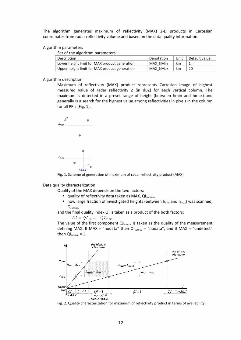
Maximum of reflectivity (MAX) product represents Cartesian image of highest

measured value of radar reflectivity Z (in dBZ) for each vertical column. The

maximum is detected in a preset range of height (between hmin and hmax) and

generally is a search for the highest value among reflectivities in pixels in the column

for all PPIs (Fig. 1).

Fig. 1. Scheme of generation of maximum of radar reflectivity product (MAX).


Quality of the MAX depends on the two factors:

� quality of reflectivity data taken as MAX, QIsource,

� how large fraction of investigated heights (between hmin and hmax) was scanned,

QIscope,


The value of the first component QIsource is taken as the quality of the measurement

defining MAX. If MAX = “nodata” then QIsource = “nodata”, and if MAX = “undetect”

then QIsource = 1.

Fig. 2. Quality characterization for maximum of reflectivity product in terms of availability.

13

The second component QIscope is determined based on heights of the highest and

lowest scans for considered Cartesian pixel (hhighest and hlowest respectively) in relation








Output



� "how": task - "pl.imgw.product2d.max",




� parameters of MAX algorithm,



� "how": task - "pl.imgw.product2d.max",



References

-

3.6. Vertically integrated liquid water

3.6.1. Quality-based vertically integrated liquid water (VIL) product generation – Product2D: VIL

Authors



Basic description


The algorithm generates vertically integrated liquid water (VIL) 2-D product from

radar reflectivity volume with quality information using product2D_PPI algorithm.


Not performed yet.

References (names and contact information)



Input data: VOL





14







Input data


� object=PVOL:





Logical steps

The algorithm generates vertically integrated liquid water (VIL) 2-D products in Cartesian

coordinates from radar reflectivity volume and based on the data quality information.




Lower height limit for VIL product generation (a.s.l.) VIL_hMin km 2

Upper height limit for VIL product generation (a.s.l.) VIL_hMax km 10

Coefficient c in Z-M formula VIL_ZMc - 24000

Coefficient d in Z-M formula VIL_ZMd - 1.82


Vertically integrated liquid water (VIL) product represents Cartesian image of the

water content residing in a user-defined layer in the atmosphere (in dBA) (Fig. 1).

Generally, in the first step a vertical profile of liquid water content M (based on Z-M

relationship) is determined by interpolation between all pairs of neighbouring

measurements. Then the VIL in a preset range of height (between hmin and hmax) is

calculated by integration of the profile. In order to find the vertical profile of M(h),

values between two measurements M’ and M” detected at heights h’ and h”

respectively, the linear interpolation is applied:

Fig. 1. Scheme of generation of vertically integrated liquid water product (VIL).

Radar reflectivity Z is related to liquid water content M (in cm3 m

-3) according to so

called Z-M relationship:

15

where constants: c = 24 000; d = 1.82 (as proposed by Selex, 2010).

The VIL (vertically integrated liquid water content) is defined as:

In the VIL algorithm there are considered only measurements (Cartesian pixels on

PPIs) between hmin and hmax, and two closest ones (below hmin and above hmax).

The following ranges of integration are considered:

� If the highest measurement is higher than hmax, then the two measurements

above and below hmax are interpolated and values of M below hmax are taken

for integration, else the integration is performed up to height of the highest

measurement.

� If the lowest measurement is lower than hmin, then the two measurements

above and below hmin are interpolated and values of M above hmin are taken

for integration, else the integration is performed with the assumption that the

lowest measurement was also at hmin.


Quality of the VIL depends on the two factors:

� quality of reflectivity data from which VIL was determined, QIsource,

� how large fraction of investigated heights (between hmin and hmax) was

scanned, QIscope,


The value of the first component QIsource is taken as an average quality of all

measurements defining VIL. If VIL = “nodata” (there is no measurement between hmin

and hmax) then QIsource = “nodata”, and if VIL = “undetect” (there is no detected

reflectivity between hmin and hmax) then QIsource = 1.

Fig. 2. Quality characterization for vertically integrated liquid water product in terms of scope.

The second component QIscope is determined based on heights of the lowest and

highest scans for considered Cartesian pixel (hlowest and hhighest respectively) in relation








16

Output



� "how": task - "pl.imgw.product2d.vil",




� parameters of VIL algorithm,



� "how": task - "pl.imgw.product2d.vil",



References

-

3.7. Ground-related precipitation, QPE

3.7.1. Networked VPR correction

Authors

Joonas Karjalainen, Jarmo Koistinen

Finnish Meteorological Institute


/dataset/what: gain, offset, nodata

Input data

Full volume scan reflectivity data(for each radar). At FMI the VPR correction for a 500 m

PseudoCAPPI composite is performed presently applying the 4 lowest elevation angles from

each radar. Other number of elevations can be applied according to the user selections.

Other data:

The classification scheme of VPRs embedded into the correction algorithm and used in real

time requires that the height of the freezing level is known at each radar site at each volume

scan moment. At FMI that is estimated from NWP nowcasting data applying the HIRLAM

model fields of temperature.

Short description

The vertical profile of radar reflectivity factor (VPR) and the measurement geometry of

weather radar introduce a vertical sampling difference between the actual precipitation at

ground level and the radar estimate of it. VPR correction is used to modify the measured

values so that they represent the precipitation conditions at ground level more accurately.

The networked VPR correction described here denotes that the correction is calculated in

radar networks so that the adjustment factor field will be continuous, not introducing

additional steps at the seam lines where measured data from neighboring radars meet.

18

3.7.2. Combination of radar-based ground precipitation rate and raingauge network data –

COMBINATION

Authors

Anna Jurczyk, Jan Szturc, Katarzyna Ośródka


Basic description

19

Final precipitation estimate is generated as combination of corrected radar-based

precipitation rate with data from raingauge. Three options/techniques are available:

− simple mean field bias (MFB),

− local-oriented MFB,

− conditional merging of the two kinds of precipitation information.


Prototype was developed and tested in the frame of RISK-AWARE Project (2003-

2007).

References



− Top-level “what”: object, data, time.

− Top-level “where”: lon, lat, projdef, xsize, ysize, xscale, yscale, LL_lon, LL_lat, UL_lon,

UL_lat, UR_lon, UR_lat, LR_lon, LR_lat.

− Dataset-specific “what”: product, gain, offset, nodata, undetect.

Input data


One of weather radar products that reflects ground precipitation rate RATE or

accumulation ACRR as IMAGE or COMP files: PPI, CAPPI, PCAPPI, MAX, etc.


Data from raingauge telemetric network.

Logical steps

Radar data is considered to be better then raingauge network in reproduction of spatial

distribution, whereas raingauges measure precipitation accurately in their locations. This

observation was a starting point of conditional merging (Sinclair and Pegram 2005). In this

approach the information from radar is used to obtain the correct spatial structure of the

precipitation field, while the field values are fitted to the raingauge observations. The

method consists of the following steps:

1. Spatial interpolation of raingauge-derived precipitation data is performed using one

of known methods (here IDW or ordinary Kriging). Resulting field is denoted as RG.

2. Next deviations between observed and interpolated radar values are calculted (RR) in

the following way:

− spatial interpolation of radar data only from pixels with raingauge locations (field

RR’),

− calculation of differences between the two maps (RR – RR’),

3. Finally spatially interpolated raingauge data is corrected using the differences (errors

of interpolation) according to the following formula:

where R’ is the merged precipitation estimate.

Gauge and radar spatial interpolation should be performed by the means of the same

method.

Two simplified techniques are available as well: simple mean field bias (MFB) and local-

oriented MFB.

Quality of merging method was evaluated applying data from May to September 2006. The

two methods of spatial interpolation, IDW and ordinary Kriging, implemented in combination

were tested. Radar data as 1-hour accumulations were employed. Raingauge set was divided

into two subsets: 1-hour accumulation data from the first one were used in combination and

from the second one for verification (10% of the whole number). Characteristics obtained

20

using IDW method are slightly better than using Kriging (e.g., RMSE equals 0.56 for IDW

whereas 0.61 for Kriging, and correlation coefficient equals 0.70 and 0.68, respectively).

Example of the algorithm running: a) radar field, b) spatially interpolated raingauge measurements, c)

spatially interpolated radar measurements from raingauge locations, d) merged field.

In Figure above an example of the conditional merging algorithm performance is shown. It

illustrates one of effects of using the technique: the combined field maintains the spatial

pattern of the radar field. Correlation coefficient between the combined field and radar one

equals 0.86 whereas between the combined field and interpolated raingauges (using IDW

method) only 0.59. On the other hand final combined rainfall field follows the mean field of

raingauge interpolation. For the whole period May–September 2006 the mean values are

0.130 mm for combined field and 0.126 mm for raingauges against 0.157 mm for radar. The

results are obtained for point data (in raingauge locations) using IDW method in

combination.

Output

− Field of adjusted precipitation rate RATE or accumulation ACRR as IMAGE or COMP

object.

− Quality index field QIND as IMAGE or COMP object.

References

− Jurczyk, A., Ośródka, K., and Szturc, J., 2008. Research studies on improvement in real-

time estimation of radar-based precipitation in Poland. Meteorol. Atmos. Phys., 101, 159-

173.

− Sinclair, S. and Pegram, G., 2005. Combining radar and rain gauge rainfall estimates using

conditional merging. Atmos. Sci. Lett., 6, 19-22.

21

3.7.3. Precipitation accumulation - ACRR

Authors

Daniel Michelson

Swedish Meteorological and Hydrological Institute

Harri Hohti

Finnish Meteorological Institute

Basic description


Derive an accumulated precipitation product based on a set of input reflectivity

products, either single-site or, more likely, composite.


Prototype developed and tested for OPERA.


scientific papers)

Sort-of based on the method used at the BALTEX Radar Data Center, but in new form.


Input

� gain, offset, nodata, and undetect for reflectivity datasets

� how/task = se.smhi.composite.distance.radar for surface distance quality indicator

fields

� gain and offset for the surface distance QI fields

Output

� Output physical parameter must have what/quantity=ACRR

� what/prodpar of the ACRR dataset must be set to the integration period (hours)

� Otherwise, metadata are the same as for input data, just that gain and offset will need

to be adjusted.

Input data


Reflectivity data are the most relevant: normally DBZH, but also TH. It's probably

unlikely that someone would want to accumulate TV or DBZV, but we might support

them too. We don't have much of a tradition of storing data as RATE (mm/h), so

these may be considered less relevant and not supported.

It is assumed here that the fixed R(Z) conversion of this algorithm is applied only until

the dynamic only conversion is available. If dynamic R(Z) conversion is applied then it

is recommended that the conversion and the accumulation are split in two separate

algorithms.

Data can be in any stage of quality. Optionally, a quality indicator dataset containing

surface distance from the radar, that accompanies a reflectivity field, can be used to

derive an average distance field that will accompany the output ACRR result.

Otherwise, it doesn't make sense to make the accumulator somehow average all the

various forms of quality indicators we may produce, at least not without careful

consideration that we won't deal with in this first version.


None



22

Required arguments

Information Type

Input data List of file names

Nominal date YYYYMMDD according to ODIM

Nominal time HHmmss according to ODIM

Nr. hours float

Images per hour integer

Proportion accepted float (0-1), e.g. 0.95 for 95%

A coefficient in Z-R float

b coefficient in Z-R float

Algorithm

It's a two-step process. Step 1 involves looping through all input images and

determining the sum of all the precipitation intensities in the time series. If the

surface distance QI field exists, also sum the distances.

A couple of notes on determining input data:

The total number of input files in the time series is (nr.hours)*(images per hour)+1.

For example, if we have an image every 15 min, there will be five images for a one-

hour accumulation.

The scheduler (Beast) will have to find input data based on the nominal date/time

which is always the end of the integration period.

It's important to use counters to keep track of how many hits in the time series there

are. This will be used in step 2 to accept or reject results. Step 1 can be illustrated

schematically as follows:

23

Step 2 takes the results of step 1 and loops one last time, using the counters to

derive ACRR results and, optionally, an associated mean distance QI field.

Schematically, this is:

24

Output

The result is an ODIM_H5 file containing a composite with an ACRR quantity and, optionally,

an associated average surface distance quality indicator field.

a) Data type using ODIM notation where possible, e.g. DBZH

� ACRR

b) Added quality indicators

� With how/task = se.smhi.composite.distance.radar

References

-

3.8. Wind speed

3.8.1. Vertical profile

Authors

Günther Haase


Basic description

The algorithm is based on the VVP method.

25


nbins, nrays, gain, offset, nodata, undetect, rscale, elangle

Input data

Polar volume or scan

Logical steps

This algorithm derives vertical profiles of reflectivity, wind speed, and wind direction from

polar volume data.

Assuming a uniform wind field the radial wind (V) has the form of a sine for constant range

and elevation angle:

where φ is the azimuth angle. The four constants are amplitude (|α|), period (2π/k), phase

shift (β), and vertical displacement (γ). The terminal velocity of the falling hydrometeors is

implicitly included in γ. For k=1 Eq. (1) yields

with

Equation (3) can be extended to n velocities which results in a nonhomogeneous matrix

equation of the form:

For more than three independent measurements, i.e. n>3, Eq. (7) is an overdetermined linear

system which can be solved using a QR factorization of A. The resulting values w1, w2, and w3

are utilized to determine α, β, and γ in Eq. (2). Squaring and adding Eqs (4) and (5) leads to

Solving Eq. (4) for α and inserting it into Eq. (5) results In

Finally, Eq. (6) provides an expression for the vertical displacement γ. Hence, Eq. (2) describes

the radial wind model which is closest to the observations. The real wind velocity is identical

with the amplitude α in Eq. (8) while the wind direction is obtained from the derivative with

respect to azimuth angle

Hence, Eq. (9) equals zero for

26

where φ1 and φ2 are the extreme values of Eq. (2). The second derivative of Eq. (2) with

respect to azimuth angle is

From Eq. (8) we know that α>0. Thus, the radial velocity in Eq. (2) has a maximum at φ1 and a

minimum at φ2. Usually the wind direction is expressed in terms of the direction from which

the wind originates (for example, a westerly wind blows from the west to the east).

Furthermore, radial velocities away from the radar (outbound) are defined as positive while

velocities towards the radar (inbound) are defined as negative. Therefore the wind direction

in the specified height layer is given by φ2.

Output

dbz, dbz_dev, ff, ff_dev, dd, n (DBZH/VRAD)

3.9. Hydrometeor classification

3.9.1. BALTRAD Hydrometer Classifier BALTRAD-HMC

Authors

Rashpal S. Gill and Martin B. Sørensen

Danish Meteorological Institute

Basic description

Pixel based hydrometeor classification is carried out using the fuzzy logic methodology (Bringi

and Chandrasekar, 2001, Zrnic et. al., 2001, Schuur et. al., 2003, Lim et. al., 2005). In the

current approach, a given pixel of hydrometeor class j has a score Sj given by the relation

where Pi and Wi are the value of the parameter i, and the associated weight, for the class j.

The radar parameters that have been used in the classifier are: ZHH, ZDR, KDP, σHV , plus the

texture parameters, associated with ZHH, ZDR, ФDP (Schuur et. al., 2003, Sugier et. al., 2006). In

fuzzy logic the values of the Pi for the different hydrometeor classes are described by the

membership functions (MF) (see section 4).

Hydrometeor classes

In the current version of the algorithm the following 12 hydrometeor classes have been

identified:

1. ground clutter,

2. sea clutter,

3. electrical signals from external emitters (EE) that interfere with our radars,

4. clean air echoes (CAE) such as from birds and insects,

5. drizzle,

27

6. light rain,

7. moderate rain,

8. heavy rain,

9. violent rain,

10. light snow,

11. moderate to heavy snow,

12. rain/hail mixture.

However, internally in the BALTRAD-HMC software there are two classes each of ground and

sea clutter, ten classes of external emitters including the signals from the sun and three

classes of CAE. Further, the light rain class consists of four sub-classes; light drizzle, moderate

drizzle, heavy drizzle and light rain.

Computational procedure

The software consists of two main modules:

1. Computation of all the radar parameters that are to be used in the fuzzy logic

classifier

2. Using fuzzy logic rules classify each pixel of the radar returned echo into one of the

predefined hydrometeor classes.

The computational procedure involves the following steps for module A:

1. from the radar volume file read in the following radar parameters: reflectivity ZHH,

differential reflectivity ZDR, cross correlation σHV, differential phase ФDP, radial velocity

Vr and spectral width W

2. by changing the default settings in the metadata file, choose whether to undertake

the following operations:

� smooth ZDR and σHV parameters, by averaging over N number of range gates,

� correct ZDR and σHV at low signal-to-noise (SNR) ratio values,

� correct ZDR and ФDP for radome effects,

� correct ZDR and ФDP for potential biases,

� compute the specific differential phase, KDP, as described in section 4 above,

� correct both ZHH and ZDR for rain attenuation as described in section 5 above.

3. now compute the following radar parameters in their appropriate units:

4. ZHH (unit dBZ) and its texture parameter, Tex(ZHH),

5. ZDR (unit dB) and its texture parameter, Tex( ZDR),

6. σHV and its texture parameter, Tex(σHV),

7. ФDP (unit deg.) and its texture parameter, Tex(ФDP),

8. KDP (unit deg./km) and its texture parameter, Tex(KDP),

9. Vr (unit m/s) and its texture parameter, Tex(Vr),

10. W (unit m/s) and its texture parameter, Tex(W),

11. signal-to-noise ratio parameter, SNR (unit dB), and

12. the top, centre and bottom heights (unit meters) of the radar beam, HTT, HTC and

HTB, respectively.

The computational procedure involves the following steps for module B:

1. read in all the computed radar parameters from module A

2. by changing the default settings in the metadata file, choose which of the above

parameters are to be used for level-1 and level-2 hydrometeor classification

3. read-in a , ß and γ indicating the centre, half- width at inflection point and the slope

of the curve of the Beta functions (see fig. 1), for each radar parameter including the

associated weights

4. for level-1 hydrometeor classification, for each radar echo

5. get the “scores “ of each of the parameter

6. using fuzzy logic rules compute the final score for each predefined classes

(precipitation, clutter, clean air echoes, and external emitters)

28

7. classify the pixel by choosing the predefined hydrometeor class with the highest

score

8. for level-2 hydrometeor classification

9. compute the heights of the melting layers using:

10. the radar volume data, and

11. from Numerical Weather Prediction (NWP) models

12. get the “scores “ of each of the parameter

13. using fuzzy logic rules compute the final score for each predefined classes (see

section 2)

14. classify the pixel by choosing the predefined hydrometeor class with the highest

score

Theoretical background

In fuzzy logic the values of the Pi, in equation (2), for the different hydrometeor classes are

described by the membership functions. In the current version the latter are expressed as

Beta functions of the type shown in fig. 1 with the 3 parameters: a, ß and γ indicating the

centre, half width at inflection point and the slope of the curve (Lim et. al., 2005).

Fig. 1 Beta membership function

As a way of example, fig. 2 shows the membership functions for the parameter ZHH for the

different classes of rain.

Fig. 2 Membership functions for ZHH for different categories of rain.

Similar membership functions exits for other hydrometeor classes for ZHH and for all the

other parameters used in the classification.

There has been much interest from international colleagues in the radar echo class 3

mentioned in section 2 above, because as far it is know, no hydrometeor classifier has

29

included a class for the external emitters before (Gill et. al., 2012). For this reason the

membership functions of ZHH ZDR and σHV for the different types of external emitters included

in the classifier are given below (fig. 3). Also note radar echoes from the sun are also a sub-

class of external emitters. Membership function of the sun plus those of external emitters for

the parameter ZHH can be seen in the bottom left part of fig. 3.

Fig. 3 Membership functions of ZHH, ZDR and rhoHV for the different types of external emitters included

in the classifier. Top left MF of a single external emitter of ZDR. Top right MF of all 9 external emitters

of ZDR . Bottom left of all 9 external emitters and of sun of ZHH. Bottom right MF of all 9 external

emitters of σHV

Examples of output from the hydrometeor classifier

The current version of the algorithm does the so-called level 1 and level 2 classifications. In

the level 1 classification a radar echo is classified into one of four simple classes:

precipitation, clutter, clean air echoes, and external emitters. Figure 4 shows an example of

the output.

Fig. 4 shows radar image on the left (ZHH original) and its corresponding level 1 hydrometeor

classification into four classes: external emitters (EE), clean air echoes (CAE), clutter and precipitation

(prec), colour code: yellow, blue, purple and green, respectively.

In the level 2 classification, the echoes that are classified as precipitation in level 1 are further

subclassified into different precipitation classes mentioned above. In this case the heights of

30

the melting layer computed by the local NWP model and/or estimated from the radar

parameters (see section 3) are used to strengthen the classification between the different

classes of rain and snow. In the current version of the level-2 classification only the

parameters ZHH, ZDR, KDP, and σHV are used. In particular, in this case score Sj is given by the

relation

Fig. 5 shows an example of the level 2 classification. Note that the radar data used to

illustrate the classifications results are the same in figures 4 and 5.

Fig. 5 shows radar image on the left (original ZHH) and its corresponding level 2 hydrometeor

classifications into eleven classes.

In addition to the above level 1 and 2 classifications, the algorithm can make use of the

above classification output to remove the non- meteorological echoes in the original radar

reflectivity product, ZHH, shown on the left in each of the figures 4 and 5. This is illustrated in

figure 6 below. Concerning the latter product, it was the first product that was requested for

routine operational use by the DMI end users, namely its meteorologists.

Fig. 6 shows the original radar product on the left and corresponding “cleaned” version on the right

which has non-meteorological echoes removed.

References

� Bringi, V.N., Chandrasekar, V., 2001. Polarimetric Doppler Weather Radar, Cambridge

Univ. Press, Cambridge, UK.

� Gill, R.S., Sørensen, M.B., Bøvith, T., Koistinen, J., Peura, M., Michelson, D., and Cremonini,

R., 2012. BALTRAD dual polarization hydrometeor classifier, ERAD 2012, 7th European

Conference on Radar in Meteorology and Hydrology.

31

� Lim, S., Chandrasekar, V., and Bringi, V.N., 2005. Hydrometeor classification system using

dualpolarization radar measurements: Model improvements and in situ verification, IEEE

Transactions of Geosciences and Remote Sensing, 43, 792-801.

� Schuur, T., Ryzhkov, A., and Heinselmann, P., 2003. Observations and classification of

echoes with the polarimetric WSR-88D radar, NOAA National Severe Storms Laboratory

Tech. Report, Norman, Oklahoma, USA.

� Sugier, J., Tabary, P., and Gourley, J., 2006. Evaluation of dual polarization technology at C

band for operational weather radar network, report of the EUMETNET OPERA II, work

packages 1.4 and 1.5.

� Zrnic, D.S., Ryzhkov, A., Straka, J., Liu Y., and Vivekanandan, J., 2001. Testing a procedure

for automatic classification of hydrometeor types, J. Atmos. Oceanic Tech, 18, 892-913.

3.9.2. Separation of convective and stratiform precipitation – CONVECTION

Authors

Anna Jurczyk, Jan Szturc, Katarzyna Ośródka


Basic description


The algorithm categorizes each radar pixel into convective or stratiform one

employing fuzzy logic approach with multi-source meteorological input data.


Prototype was developed and tested in the frame of grant awarded by Polish

Ministry of Science and Higher Education (2009-2012)


scientific papers)



Input data

If input data: object=PVOL

• General “what”: source(NOD).

• For particular SCANs:

o Dataset-specific “where” for data and QI: nbins, nrays.

o Data-specific “what” for data: gain, offset, nodata, undetect.

o Data-specific “what” for QI: gain, offset, nodata, undetect.

If input data: object=IMAGE

• Top-level “what”: object, data, time.

• “Where”: lon, lat, projdef, xsize, ysize, xscale, yscale, LL_lon, LL_lat, UL_lon,


• Dataset-specific “what” for data: product.

• Data-specific “what” for data: gain, offset, nodata, undetect.

• Data-specific “what” for QI: gain, offset, nodata, undetect.


• Top-level “what”: object, data, time.

• “Where”: lon, lat, projdef, xsize, ysize, xscale, yscale, LL_lon, LL_lat, UL_lon,


• Dataset-specific “what” for data: product.

• Data-specific “what” for data: gain, offset, nodata, undetect.

• Data-specific “what” for QI: gain, offset, nodata, undetect.

32

Input data


• object=PVOL (quantity=DBZH/TH) or three object=IMAGE: product=MAX

(quantity=DBZH), VIL (quantity=VIL), ETOP (quantity=HGHT).


• Meteosat products: Cloud Type; Overshooting Tops.

• Lightning detection data: Number of cloud-to-ground lightning.

• NWP model data: Convective Available Potential Energy (CAPE); Total Totals

Index (TTI).

Logical steps

The algorithm for separation of convective and non-convective precipitation is based on

multi-source meteorological data.


Table 1. Set of the algorithm parameters (for standard version)

Description Denotation Default

value

Preliminary threshold for convection (dBZ) ThresholdConv 25

Lower threshold for convection area (km2) ThresholdAreaConv 4

Weight for member function of MAX for C class in fuzzy logic

scheme

MaxPar_weightC 0.3

Weight for member function of MAX for S class in fuzzy logic

scheme

MaxPar_weightS 0.3

Weight for member function of MAXDiff for C class in fuzzy logic

scheme

MaxDiff_weightC 0.4

Weight for member function of MAXDiff for S class in fuzzy logic

scheme

MaxDiff_weightS 0.4

Weight for member function of ETOP for C class in fuzzy logic

scheme

EtopPar_weightC 0.15

Weight for member function of ETOP for S class in fuzzy logic

scheme

EtopPar_weightS 0.15

Weight for member function of VILDiff for C class in fuzzy logic

scheme

VilDiff_weightC 0.15

Weight for member function of VILDiff for S class in fuzzy logic

scheme

VilDiff_weightS 0.15

Radius for MAXDiff and VILDiff determination (km) ConvRadius 11

Code for convective pixels (between 1 and 255) CodeC 2

Code for stratiform (non-convective) pixels (between 1 and 255) CodeS 1

Input data

Table 2. The list of the algorithm input data (selected empirically).

Input data Units Description

Weather radar products

Maximum of reflectivity (Z) dBZ Product: MAX(Z) – Maximum. Display range of height:

1–15 km

Height of radar echo top (ET) km Product: EHT(Z) – Echo Height. Echo threshold: 4 dBZ

Water content in atmosphere

(VIL)

mm Product: VIL – Vertically Integrated Liquid. Range of

height: 1–10 km

Weather radar-based

parameters

Difference of reflectivity (ΔZ =

Zmax / Zmean)

dBZ Calculated from MAX(Z) radar product

Difference of VIL (ΔVIL = VIL / mm Calculated from VIL radar product

33

VILmean)

Meteorological satellite

products

Cloud Type (CT) (classes) EUMETSAT product

Overshooting Tops (OTS) K EUMETSAT product

Lightning detection system

products

Cloud-to-ground lightning (CG) (number) Calculated from reports generated every 1 minute that

include data about each lightning

Numerical weather prediction

products

Convective Available Potential

Energy (CAPE)

J kg-1

Based on thermodynamic diagram

Total Totals Index (TTI) °C Based on thermodynamic diagram

The radar data are mandatory for the algorithm correct running. The two options of

input data set are available:

• option standard: using only radar data as input (five first parameters from

Table 2),

• option standard+: using all set of input data (Table 2) - to be implemented.

Separation of convective and non-convective precipitation

The identification of convection areas is performed by fuzzy logic approach, which is

applied to categorize each radar pixel into convective or non-convective precipitation

(classes: non-convective S, or convective C). For the both classes membership

functions are defined for all selected parameters. Then the functions are aggregated

as weighted sums:

where: x is the precipitation class (S or C); i is the parameter number; n is the number

of the parameters; Pxi is the membership function for i-th parameter; Wxi is the

weight of i-th parameter. Comparison of the weighted sums for both classes decides

which category S or C a considered radar pixel belongs to.

The membership functions were determined on Polish meteorological data set from

2007 and 2013. The whole data set was labelled by hand as convective or non-

convective areas, which was done by meteorologist from forecast office as a human

expert. In this way two data subsets were created with all parameter values, and

then membership functions were empirically established for all parameters.

34

Two kinds of the functions were employed: one- and two-dimensional (1-D and 2-D),

the latter for the parameters that are calculated from two other ones (i.e. ΔZ and

ΔVIL).

The 1-D membership functions were obtained from analyses of scatter diagrams for

the particular parameters (Fig. 1), which allowed to determine threshold values

above or below which the values of relevant membership functions are attributed to

0 or 1, and linear or another approximation of the function values within the range

(0, 1).

35

Fig. 1. One-dimensional membership functions for convective (on the left) and stratiform (on

the right) precipitation.

The 2-D membership function is defined not for single parameter but for two

parameters analysed jointly: (ΔZ, Z) and (ΔVIL, VIL). Membership functions for C and S

classes were determined in dependence on certain percentiles empirically estimated

on historical data. The uncertainty area was assumed to lay between 5% and 25%-

percentiles of all parameters’ pairs gathered in appropriate data subset, as it is

presented in Fig. 2. For values below 5% and above 25%-percentile values of

membership functions were assigned to 0 and 1 respectively, whereas for values

between 5% and 25%-percentile values of membership function are linearly

interpolated in range from 0 to 1 taking distances to the both percentiles into

account. In our case for two investigated 2-D membership functions it turned out

36

that 5%-percentiles for convective and non-convective classes are so close each other

that they were approximated by the common one.

Fig. 2. Two-dimensional membership functions for ΔZ (on the left) and ΔVIL (on the right).

Quality characterization

Map of quality index (QI) will be calculated for the output field. The QI will be

determined based on comparison of PC and PS - sums of membership functions for

thw two classes: convective and non-convective precipitation.

Example

Example of radar reflectivity field in dBZ (on the left) and detected area of convective

and stratiform precipitation (on the right) for Legionowo radar (12 August 2007, 14

UTC):

Output


Output quantity CLASS (convective/non-convective precipitation) as IMAGE object (in

Cartesian coordinates) with:

• "how": task - "pl.imgw.product2d.convection",

• "how": task_args - parameters of CONVECTION algorithm.



• "how": task - "pl.imgw.product2d.convection",

• "how": task_args - parameters of CONVECTION algorithm.

References

37

− Scientific paper: Jurczyk, A., Szturc, J., and Ośródka, K., 2012. Convective cell

identification using multi-source data. IAHS Publ., no. 351, 360-365.

4. Quality-related data processing

For the 3D volumes (PVOL in ODIM denotation) postprocessing a set of quality algorithms has been

designed and developed, which are dedicated to the data corrections. As a result the corrected

(quality enhanced) volumes with related quality information (as quality index, QI) can be used for

generation of more reliable 2D products. The quality algorithms for volume postprocessing are

available in BALTRAD toolbox.

4.1. Brief catalogue of quality algorithms for 3D reflectivity data volumes

4.1.1. Removal of geometrically-shaped non-meteorological echoes and quality characterization

(as a part of RADVOL-QC package) – RADVOL-QC: SPIKE

Authors




� Dataset-specific “what”: gain, offset, nodata, undetect.

� Dataset-specific “where”: elangle, nbins, nrays, rscale.

Input data

object=PVOL or SCAN; quantity=DBZH, otherwise TH.

Short description

The spurious echoes from sun and external interference, so called spikes, are characterized

by their spatial structure that clearly differs from precipitation field pattern. The shape of

such echo is very specific: it is similar to a spike along the whole or large part of a single or a

few neighbouring radar beams. Reflectivity field structure is investigated to detect such echo

on radar image in this algorithm, which identifies spikes, cuts them out from the precipitation

field, and replaces by proper reflectivity values.

In the algorithm two stages of spike removal are introduced: for “wide” (subalgorithm A) and

“narrow” (subalgorithm B) types of spikes.

Output

Data type using ODIM notation where possible

Corrected DBZH, with "pl.imgw.radvolqc.spike" added to data-specific "how"/task,

and the algorithm parameters added to "how"/task_args.


Quality index (QI = 0 for bad data, QI = 1 for excellent data) with

"pl.imgw.radvolqc.spike" in quality-specific "how"/task, and the algorithm

parameters in "how"/task_args.

4.1.2. Removal of non-meteorological echoes and quality characterization – RADVOL-QC: NMET

Authors



38


� Top-level “where”: height.



Input data


Short description

In the detector two stages of non-meteorological echo removal are introduced: for “low”

(subalgorithm A), and “high” (subalgorithm B) types of the echoes.

Output

a) Data type using ODIM notation where possible

Corrected DBZH, with "pl.imgw.radvolqc.nmet" added to data-specific "how"/task,


b) Quality index (QI) field


"pl.imgw.radvolqc.nmet" in quality-specific "how"/task, and the algorithm


4.1.3. Removal of measurement noise and quality characterization – RADVOL-QC: SPECK

Authors






Input data


Short description

Generally, the specks are isolated radar gates with or without echo.

Output

Data type using ODIM notation where possible

Corrected DBZH, with "pl.imgw.radvolqc.speck" added to data-specific "how"/task,




"pl.imgw.radvolqc.speck" in quality-specific "how"/task, and the algorithm


4.1.4. Quality characterization due to distance to radar related effects – RADVOL-QC: BROAD

Authors



39


� Top-level “how”: beamwidth, pulsewidth.



Input data


Short description

The horizontal and vertical broadening of radar beam for each gate can be computed when

its polar coordinates are known: elevation angle, azimuth angle, and radial distance to radar

site in km, and two parameters of radar beam: beam width and measurement gate length in

km calculated from radar pulse length.

Output


-



"pl.imgw.radvolqc.broad" in quality-specific "how"/task, and the algorithm


4.1.5. Correction of partial and total beam blockage and quality characterization including ground

clutter – RADVOL-QC: BLOCK

Authors




� Top-level “where”: height.

� Top-level “how”: beamwidth.



Input data

object=PVOL; quantity=DBZH, otherwise TH.

Short description

A geometrical approach is applied to calculate the degree of the beam blockage.

Output


Corrected DBZH, with "pl.imgw.radvolqc.block" added to data-specific "how"/task,




"pl.imgw.radvolqc.block" in quality-specific "how"/task, and the algorithm parameters in "how"/task_args.

40

4.1.6. Correction and quality characterization for attenuation in rain – RADVOL-QC: ATT

Authors






� Dataset-specific “where”: nbins, nrays, rscale.

Optional:

� General “how”: wavelength (needed if parameters ATT_a and ATT_b do not exist in XML

parameter file).

Input data


Short description

Reflectivity-based algorithm is used iteratively (“gate by gate”) for correction of attenuation

in rain.

Output


Corrected DBZH, with "pl.imgw.radvolqc.att" added to data-specific "how"/task, and

the algorithm parameters added to "how"/task_args.



"pl.imgw.radvolqc.att" in quality-specific "how"/task, and the algorithm parameters

in "how"/task_args.

4.1.7. Polarimetric rain attenuation correction : rainATTENcorrect

Authors

Rashpal S. Gill and Martin B. Sørensen

Danish Meteorological Institute

1. Algorithm name

Rain attenuation correction of reflectivity an differential reflectivity: PolRainAttCorr

2. Basic description

A number of methods have been proposed in the literature for correcting ZHH for rain

attenuation (Bringi el. al., 1990, Carey et al., 2000, Tesud et. al., 2000, Bringi et al., 2001).

Describing each one of these is beyond the scope of this report. However, it is suffice to state

that from an operational point of view, the so-called “Linear ФDP with a fixed linear α”, by

Bringi et. al., (1990) is preferred as it is easy to implement in real-time and is not too

demanding computationally. However, its main dis-advantage is that it can over or under-

estimate attenuation. In the current version of the software, this method has been

implemented to correct for the attenuation suffered by ZHH and ZDR in rain.

3. Computational procedure

41

Similar to computing KDP, correcting ZHH and ZDR for rain attenuation is rather challenging as

the underlying ФDP(r) are very “noisy” i.e., generally contain many outliers. The current

method used at DMI was inspired by Bringi et. al. (2005) and involve the following steps:

1. Compute the texture of ФDP, Tex( ФDP(x,y)), using equation (2).

2. Generate range mask based on thresholds for Tex(ФDP(x,y)threshold), Signal-to-Noise Ratio

(SNRthreshold) and ρHVthreshold to remove bad ФDP values.

3. Interpolate ФDP across “bad” data segments.

4. Compute the ФDP(0) i.e., offset at the “origin” by averaging the first N range gates FDP

containing precipitation.

5. ФDP(r) is then smoothed using a median filter with a window size of ~ 5.0 km - 6.5 km.

6. Correct both ZHH and ZDR for rain attenuation using equations (13) and (16), respectively.

4. Theoretical background

For an inhomogeneous path, i.e. Ah varies along the path, the corrected ZHH (units of dB) is

related to the measured measured ZHH at range r from the radar by the following expression

Substituting equation (10) into the above expression and assuming a is constant we get

Now substituting for KDP from equation (1), the following expression is obtained for the

corrected ZHH

Thus knowing by how much ФDP increases from its value at the origin ФDP(0) it is possible to

correct the radar reflectivity, ZHH,

Radar differential reflectivity rain attenuation correction

Just like the above radar horizontal reflectivity, ZHH , the differential reflectivity also suffer

from rain attenuation, especially at C- and X-bands. To estimate the rain attenuation of ZDR,

we repeat the above procedure for ZHH. We get in this case the following expression

where ADP is the difference between the specific attenuations between the horizontally and

vertically polarized waves, i.e., ADP = AH - AV , and is normally referred to as the specific

42

differential attenuation. By analogy to equation (10) a linear relationship between ADP and

KDP has been proposed (Bringi et. al., 1990) i.e.,

Substituting equation (15) into (14) we get the following expression for the corrected ZDR

The coefficient β is typically 0.01-0.003 at C-band (Bringi et. al., 2005).

References

� Bringi V. N., Chandrasekar N., Balakrishnan and Zrnic D. S., 1990, ”Anexamination of

propagationeffects in rainfall on radar measurements at microwave frequencies”, J.

Atmos. Oceanic Tech.,vol., 7, 829 – 840.

� Bringi, V. N., Chandrasekar, V.: 2001, ”Polarimetric Doppler Weather Radar”, Cambridge

Univ.press, Cambridge, UK.

� Bringi V. N., Thurai R., and Hannesen R., 2005, “Dual-Polarization Weather Radar

Handbook”,AMS-Gematronik GmbH.

� Carey L. D., Rutledge S. A., Ahijevych D. A., and Keenan T. D., 2000, “ Correcting

propagationeffects in C-band polarimetric radar observations of tropical convection using

differential propagationphase”, J. Appl. Meteor., vol. 39, 1405 – 1433.

Short description

A number of methods have been proposed in the literature for correcting ZHH for rain

attenuation. Describing each one of these is beyond the scope of this report. However, it is

suffice to state that from an operational point of view, the so-called “Linear ФDP with a fixed

linear α” is preferred as it is easy to implement in real-time and is not too demanding

computationally. However, its main disadvantage is that it can over or under-estimate

attenuation. In the current version of the software, this method has been implemented to

correct for the attenuation suffered by ZHH and ZDR in rain.

4.2. Brief catalogue of quality algorithms for 3D Doppler data volumes

4.2.1. Dealiasing radial winds

Authors

Günther Haase



nbins, nrays, gain, offset, nodata, undetect

Input data

Polar volume or scan

43

Short description

The algorithm detects abrupt velocity changes between neighboring measurements and

eliminates (multiple) folding.

Output

VRAD

References to quality algorithms

Bringi, V.N., Chandrasekar, N., Balakrishnan, and Zrnic, D. S., 1990. An examination of propagation

effects in rainfall on radar measurements at microwave frequencies, J. Atmos. Oceanic Tech.,

7, 829 – 840.

Bringi, V.N., Chandrasekar, V., 2001, Polarimetric Doppler Weather Radar, Cambridge Univ. Press,

Cambridge, UK.

Bringi, V.N., Thurai, R., and Hannesen, R., 2005. Dual-Polarization Weather Radar Handbook, AMS-

Gematronik GmbH.

Carey, L.D., Rutledge, S.A., Ahijevych, D.A., and Keenan T.D., 2000. Correcting propagation effects in

C-band polarimetric radar observations of tropical convection using differential propagation

phase, J. Appl. Meteor., 39, 1405 – 1433.

Haase G. and Landelius T., 2004: De-aliasing of Doppler Radar Velocities Using a Torus Mapping. J.

Atmos. Oceanic Technol., 21, 1566-1573.

Michelson, D.B., Lewandowski, R., Szewczykowski, M., Beekhuis, H., 2009. EUMETNET OPERA

weather radar information model for implementation with the HDF5 file format. OPERA

Working Document WD_2008_03.

Ośródka, K., Szturc, J., Jurczyk, A., 2012. Chain of data quality algorithms for 3-D single-polarization

radar reflectivity (RADVOL-QC system). Meteorol. Appl. (Early view).

Szturc, J., Michelson, D., Koistinen, J., Haase, G., Plura, M., Gill, R., Sorensen, M., Ośródka, K., Jurczyk,

A., 2012a. Data quality in the BALTRAD+ project. Proc. 7th European Conference on Radar in

Meteorology and Hydrology ERAD 2012, Toulouse, France (CD).

Szturc, J., Ośródka, K., Jurczyk, A., 2012b. Quality control algorithms applied on weather radar

reflectivity data. In: Doppler Radar Observations – Weather Radar, Wind Profiler, Ionospheric

Radar, and Other Advanced Applications, (Eds. J. Bech and J. L. Chau), InTech, 289–306.

4.3. Total quality characterization

Part of the quality algorithms apart from corrections generates quality index QI fields that represents

quality related to particular quality factors. In order to obtain total QI field characterizing quality

because of all factor, another algorithm should be applied.

4.3.1. Total quality index (QI) for scans/volumes – QI_TOTAL

Basic description


Integration of quality indices generated by all or selected quality algorithms.


Not developed yet.


scientific papers)




44

� Dataset-specific “what” for QI data: gain, offset, nodata, undetect.

� Dataset-specific “where” for QI data: nbins, nrays.

Input data


object=PVOL or SCAN; quantity=QIND (QI information generated by particular quality

algorithms).


None.



Quality Index (QI) definition

Quality index QI is a unitless quantity with values in the range from 0 to 1, where: QI

= 0 for bad data, QI = 1 for excellent data.



Description Denotation Available options Default

value

List of QI fields QIFields Example: “pl.imgw.radvoqc.att,

pl.imgw.radvolqc.spike”;

NULL means all available QI

fields

NULL (all

available)

Methods of

combination of

particular QIs into

total QI

Method multi / add / min multi

Overwrite if total QI

already exists

Overwrite 0 (no) / 1 (yes) 0

At first the XML file is checked whether there exists group for a considered radar

(based on the radar name read from "what"/source(NOD)), which contains the

algorithm parameters. If "yes", then parameters are read from that XML group, but if

it is impossible for a particular parameter, then default value from source code is

taken. If the group does not exist, parameters are read from <default> group in XML

file in analogous way.

If the algorithm is run by means of BALTRAD toolbox then all the algorithm

parameters for each specific radar should be placed in relevant XML file by the

BALTRAD system admin. Default parameters are placed in the file by admin as well.

Moreover, the algorithm default parameters are also included in software.

Computation

Total quality index is generated from all or selected quality indices earlier generated

by BALTRAD quality algorithms. It constitutes the final stage in data volumes

processing.

The total QI is generated:

� from all QI fields available in quality fields (quantity=QIND),

� from QI fields selected for particular quality algorithms ("how": task).

45

If there are no available particular QI fields then total QI is not generated. If a given

pixel is marked as "nodata" value at least in one of QI fields then "nodata" is assigned

to total QI as well.

The following methods for the QIs combination are to select:

� multi (multiplicative)

� add (additive)

� min (minimum value)

where i = 1, …, n; n is the number of particular quality indices.

Output

a) Data type using ODIM notation where possible, e.g. DBZH

No changes.


Total quality index QI with:

� "pl.imgw.qi_total" in quality-specific "how": task,

� combination method and the particular contributing QIs listed in "how":

task_args.

5. Data visualization

5.1. BALTRAD WMS

Authors

Tuomas Peltonen, Juhani Lahtinen

STUK

Basic description

Web Map Service

WMS (Web Map Service) is a standard protocol for serving georeferenced images

over the Internet developed and published by the Open Geospatial Consortium

(OGC). Images are generated on the server side. There are available a lot of software

that has support for WMS. Examples include OpenLayers for Web browser usage and

Quantum GIS for desktop usage.

Technical description

Software is independent of BALTRAD node. Only ODIM HDF5 or GeoTIFF files are

needed for data input. Software consist of Python scripts based on Mapserver

software. The main program is the visualization script which runs via Web server.

There is also data converter script that converts from HDF5 files to GeoTIFF raster

images. Installation instructions are included in the GIT repository.

Metadata requirements

Projection must be defined in ODIM metadata.

The software has also support for FMI Open data.

Output

Output for WMS clients

Mapserver supports many different output formats that can be requested via WMS

client.

Georeferenced GeoTIFF images

Geotiff images can also be downloaded using the software. These images can be

useful if are viewed or edited in a GIS software.

46

KMZ files

Software also has capability to generate KMZ files that can be viewed in Google

Earth. It is possible to create a KMZ file with either a single image or time series.

Example of usage in (STUK)

Software is integrated into the collaborative emergency management software "TIUKU" and

dose-rate monitoring network web interface "USVA". The integration allows viewing of radar

images together with dispersion model or measurement results.

6. Abbreviations

2D – two-dimensional

3D – three-dimensional

ACL – application case logs

ATC – air traffic control

CAPPI – constant altitude plan position indicator (standard radar product)

ETOP – echo top (standard radar product)

IMAGE – 2-D Cartesian image (file object)

LAWR – local area weather radar (type of weather radar)

MAX – maximum of reflectivity (standard radar product)

NWP – numerical weather prediction

ODIM – OPERA digital information model

PPI – plan position indicator (standard radar product)

PVOL – polar volume (file object)

QI – quality index

QIND – quality index (quantity identifier)

R – precipitation rate/accumulation

SCAN – polar scan (file object)

SRI – surface rainfall intensity (standard radar product)

V – wind data (velocity and direction)

47

VAD – velocity azimuth display (standard radar product)

VIL – vertically integrated liquid water (standard radar product)

VVP – volume velocity processing (standard radar product)

Z – radar reflectivity

7. References

Michelson, D. B., Lewandowski, R., Szewczykowski, M., Beekhuis, H., 2011. EUMETNET OPERA

weather radar information model for implementation with the HDF5 file format, Version 2.1.

OPERA Working Document WD_2008_03.

Szturc, J., Ośródka, K., Jurczyk, A., Maksym, J., 2009. Definition of the target end-users. BALTRAD

Project document W701.

Szturc, J., Ośródka, K., Jurczyk, A., Maksym, J., 2010. The end-users requirements and expectations.

BALTRAD Project document W702.

Szturc, J., Ośródka, K., Szewczykowski, M., Jurczyk, A., Lahtinen J., 2012. Report on Application Case

Log. BALTRAD Project document W703 (see also BALTRAD project webpage:

http://baltrad.eu/what-baltrad-offers-you).

Szturc, J., Ośródka, K., Jurczyk, A., Lahtinen, J., 2012. Draft of catalogue of radar-based products

which end-users are interested in. BALTRAD Project document W402.

Report on radar-based products developed in the frame of...

Documents

Transcript of Report on radar-based products developed in the frame of...