Report on Integration and Evaluation Results · D6.3 Report on Integration and Evaluation Results...
131
D6.3 Report on Integration and Evaluation Results – Dissemination Level: Public Page 1 GRANT AGREEMENT No 609035 FP7-SMARTCITIES-2013 Real-Time IoT Stream Processing and Large-scale Data Analytics for Smart City Applications Collaborative Project Report on Integration and Evaluation Results Document Ref. D6.3 Document Type Report Workpackage WP6 Lead Contractor AI Author(s) Mirko Presser, João Fernandes (AI), Daniel Kuemper, Thorben Iggena, Marten Fischer (UASO), Payam Barnaghi, Nazli Farajidvar, Sefki Kolozali (UNiS), Thu-Le Pham, Muhammad Intizar Ali (NUIG), Dan Piui (SAGO) Contributing Partners AI, UASO, UniS, ERIC, SIE, AA Planned Delivery Date M36 Actual Delivery Date 21 st October 2016 Dissemination Level Public Status Final Version V1.0 Reviewed by NUIG
Transcript of Report on Integration and Evaluation Results · D6.3 Report on Integration and Evaluation Results...

D6.3 Report on Integration and Evaluation Results – Dissemination Level: Public Page 1
GRANT AGREEMENT No 609035 FP7-SMARTCITIES-2013
Real-Time IoT Stream Processing and Large-scale Data Analytics for Smart City Applications
Collaborative Project
Report on Integration and Evaluation Results
Document Ref. D6.3
Document Type Report
Workpackage WP6
Lead Contractor AI
Author(s)
Mirko Presser, João Fernandes (AI), Daniel Kuemper, Thorben Iggena, Marten Fischer (UASO), Payam Barnaghi, Nazli Farajidvar, Sefki Kolozali (UNiS), Thu-Le Pham, Muhammad Intizar Ali (NUIG), Dan Piui (SAGO)
Contributing Partners AI, UASO, UniS, ERIC, SIE, AA
Planned Delivery Date M36
Actual Delivery Date 21st October 2016
Dissemination Level Public
Status Final
Version V1.0
Reviewed by NUIG

D6.3 Report on Integration and Evaluation Results – Dissemination Level: Public Page 2
Executive Summary This report presents the technical evaluation of the CityPulse Smart City framework, specifically its
software components. Overall, the CityPulse framework delivers where other platforms and projects
have shown shortcomings, as presented in the table below.
IoT Smart City Platforms and their supported features
iCity Smart Santandler
OpenIoT
iCore SpitFire
PLAY Star City VITAL CityPulse
IoT Data Collection Semantic Interoperability
Event Detection and Data Analytics
Application Development Support
The CityPulse framework integrates and processes large volumes of streaming city data in a flexible
and extensible way. Service and application creation is facilitated by open APIs that are exposed by
CityPulse components. The framework consists of (1) Large scale data stream processing modules
and (2) Adaptive decision support modules.
The project has created and maintained a code repository to make all of the modules available as
software code under open source licenses. The core components are listed below.
The majority of this report (section 3) is looking into the quantitative performance of each the
components.
Repository Title Description Type
Quality Explorer
The Quality Explorer is a web‐based tool to get detailed insight about the quality of information the deploy sensors provide.
Component
Resource Manager The Resource Management component in the CityPulse framework is responsible for managing all Data Wrappers. During runtime an application developer or the CityPulse framework operator can deploy new Data Wrappers to include data from new data streams.
Component
Composite Monitoring
Composite Monitoring and Evaluation Code. The Composite Monitoring Component is used to evaluate correlations between individual data streams. It is used to check the plausibility of space‐time congruent data sets.
Component
Geospatial Data Infrastructure
The Geospatial Data Infrastructure (GDI) component is used by a number of other CityPulse components to tackle geo‐spatial tasks.
Component
Knowledge Acquisition Toolkit 2.0
The Knowledge Acquisition Tool (KAT) is a software toolkit that implements the state‐of‐the‐art machine learning and data analytic methods for sensors data.
Component

D6.3 Report on Integration and Evaluation Results – Dissemination Level: Public Page 3
The algorithms and methods implemented in KAT are used for processing and analysing the smart city data in the CityPulse project.
Stream Discovery and Integration Middleware
The Stream Discovery and Integration Middleware is a middleware for complex event services. It is implemented to fulfill large‐scale data analysis requirements in the CityPulse project and is responsible for event service discovery, composition, deployment, execution and adaptation.
Component
Social Media Analyser This is package includes a php subpackage for Twitter data collection via connection to streaming API, a python Annotation GUI for labelling the collected data and finally a Twitter analysis sub‐package in python and java that are used in the CityPulse project.
Component
Fault Recovery The Fault recovery component ensures the continuous and proper operation of the CityPulse enabled application by generating estimated values for the data stream when the quality drops or it has temporally missing observations.
Component
IoT Framework A mechanism for converting data points stored in the IoT‐Framework into semantically annotated data. This can be used for searching and accessing raw sensory data in a smart city data analytics framework.
Component
Decision Support and Contextual Filtering
The Decision Support component utilises contextual information to provide optimal solutions of smart city applications. The Contextual Filtering component continuously identifies and filters critical events that might affect the optimal result of the decision making task.
Component
Event Detector The Event Detection component provides the generic tools for processing the annotated as well as aggregated data streams to obtain events occurring into the city. This component is highly flexible in deploying new event detection mechanisms, since different smart city applications require different events to be detected from the same data sources.
Component
SAOPY SAOPY is a sensor annotation library that embodies well‐known ontologies in the domain of sensor networks that are used in the CityPulse project. It enables to prevent common syntax errors (e.g. undefined properties and classes, poorly formed namespaces, problematic prefixes, literal syntax) in RDF documents during the annotation process before it is published as linked data.
Component

D6.3 Report on Integration and Evaluation Results – Dissemination Level: Public Page 4
Table of contents
1 Introduction .................................................................................................................................. 11
1.1 Smart City Frameworks ....................................................................................................... 12
2 CityPulse Framework Components and Integrated Demonstrator .............................................. 15
2.1 Software components and scenarios .................................................................................. 15
2.2 SmartCity Demonstrator ..................................................................................................... 18
2.2.1 CityPulse Framework .................................................................................................... 18
2.2.1.1 Large scale data stream processing modules ......................................................... 19
2.2.1.2 Resource Management .......................................................................................... 21
2.2.1.3 Data Aggregation .................................................................................................... 22
2.2.1.4 Data Federation ...................................................................................................... 23
2.2.1.5 Event Detection ...................................................................................................... 24
2.2.1.6 Qualitative Monitoring ........................................................................................... 27
2.2.1.7 Fault Recovery ........................................................................................................ 29
2.2.1.8 Geo‐spatial database .............................................................................................. 30
2.2.1.9 City Dashboard ....................................................................................................... 31
2.2.2 Real-time Adaptive Urban Reasoning ........................................................................... 32
2.2.2.1 Contextual Filtering ................................................................................................ 33
2.2.2.2 Event‐based User‐Centric Decision Support .......................................................... 35
2.2.2.3 Technical Adaptation .............................................................................................. 38
2.2.3 Components interdependencies ................................................................................... 39
2.2.4 Context-Aware Real Time Travel Planner .................................................................... 39
2.2.4.1 Large‐scale data stream processing workflow ....................................................... 40
2.2.4.2 Real‐time Adaptive Urban Reasoning for Travel Planner ....................................... 43
3 Performance Evaluation ................................................................................................................ 49
3.1 KPIs ...................................................................................................................................... 49
3.1.1 Observation Point KPIs ................................................................................................. 49
3.1.2 Network Connection KPIs ............................................................................................. 49
3.1.3 Data Processing Related KPIs ...................................................................................... 50
3.2 Component Evaluations ...................................................................................................... 52
3.2.1 QoI Annotation .............................................................................................................. 52
3.2.1.1 Overview ................................................................................................................. 53
3.2.1.2 Testing .................................................................................................................... 54

D6.3 Report on Integration and Evaluation Results – Dissemination Level: Public Page 5
3.2.1.3 Measurements........................................................................................................ 54
3.2.1.4 Conclusion .............................................................................................................. 58
3.2.2 Composite Monitoring ................................................................................................... 59
3.2.2.1 Testing .................................................................................................................... 59
3.2.2.2 Overview ................................................................................................................. 60
3.2.2.3 Measurements........................................................................................................ 60
3.2.2.4 Processing Capacity ................................................................................................ 61
3.2.3 Fault recovery ................................................................................................................ 62
3.2.3.1 Overview ................................................................................................................. 62
3.2.3.2 Testing .................................................................................................................... 62
3.2.3.3 Measurements........................................................................................................ 63
3.2.3.4 Conclusion .............................................................................................................. 65
3.2.4 Event detection .............................................................................................................. 66
3.2.4.1 Overview ................................................................................................................. 66
3.2.4.2 Testing .................................................................................................................... 66
3.2.4.3 Measurements........................................................................................................ 67
3.2.4.4 Conclusion .............................................................................................................. 69
3.2.5 Semantic Annotation ..................................................................................................... 69
3.2.5.1 CityPulse Information Model .................................................................................. 70
3.2.5.2 Pre‐semantic validation with the Sensor Annotation Library: SAOPY.................... 71
3.2.5.3 Post‐semantic validation with the SSN Validation Tool ......................................... 71
3.2.5.4 The Ontology Validations ....................................................................................... 72
3.2.5.5 Discussion ............................................................................................................... 74
3.2.6 Data Aggregation .......................................................................................................... 74
3.2.6.1 Time ........................................................................................................................ 75
3.2.6.2 CPU ......................................................................................................................... 78
3.2.6.3 Data size ................................................................................................................. 80
3.2.6.4 Reconstruction Rate ............................................................................................... 80
3.2.6.5 Influence of the SensorSAX parameters ................................................................. 81
3.2.6.6 Discussions ............................................................................................................. 83
3.2.7 Contextual Filtering ....................................................................................................... 86
3.2.7.1 Overview ................................................................................................................. 87
3.2.7.2 Testing .................................................................................................................... 87

D6.3 Report on Integration and Evaluation Results – Dissemination Level: Public Page 6
3.2.7.3 Measurements........................................................................................................ 87
3.2.7.4 Conclusion .............................................................................................................. 89
3.2.8 Reward and Punishment algorithm for normalised QoI metrics ................................... 89
3.2.8.1 RAM Utilisation ....................................................................................................... 89
3.2.8.2 Processing Capacity ................................................................................................ 90
3.2.9 Decision Support ........................................................................................................... 91
3.2.9.1 Overview ................................................................................................................. 92
3.2.9.2 Testing .................................................................................................................... 92
3.2.9.3 Measurements........................................................................................................ 93
3.2.9.4 Conclusion .............................................................................................................. 95
3.2.10 TestFramework ............................................................................................................. 95
3.2.10.1 Testing .................................................................................................................... 95
3.2.10.2 Overview ................................................................................................................. 96
3.2.10.3 Measurements........................................................................................................ 96
3.2.10.4 Conclusion .............................................................................................................. 99
3.2.11 Data Federation ............................................................................................................. 99
3.2.11.1 Overview ................................................................................................................. 99
3.2.11.2 Testing .................................................................................................................. 100
3.2.11.3 Measurements...................................................................................................... 100
3.2.11.4 Conclusion ............................................................................................................ 108
3.2.12 Technical Adaptation ................................................................................................... 109
3.2.12.1 Overview ............................................................................................................... 109
3.2.12.2 Testing .................................................................................................................. 109
3.2.12.3 Measurements...................................................................................................... 110
3.2.12.4 Conclusion ............................................................................................................ 114
3.2.13 Social Media Data Evaluations ................................................................................... 114
3.2.13.1 Experiments and Results I .................................................................................... 114
3.2.13.2 Experiments and Results II ................................................................................... 118
4 Conclusions ................................................................................................................................. 123
5 References .................................................................................................................................. 127
D6.3 Report on Integration and Evaluation Results – Dissemination Level: Public Page 7
List of Figures Figure 1: The components of the CityPulse framework with their APIs. .............................................. 19
Figure 2: Data wrapper modules and processing chain. ....................................................................... 20
Figure 3: CityPulse information model. ................................................................................................ 21
Figure 4: Architecture of Data Federation ............................................................................................ 24
Figure 5: Event detection node ............................................................................................................. 25
Figure 6: Social Media stream processing and event detection component ....................................... 26
Figure 7: QoI Explorer ........................................................................................................................... 28
Figure 8: Composite Monitoring Process .............................................................................................. 29
Figure 9: Fault recovery component workflow. .................................................................................... 30
Figure 10: Weighting Edges On a Street Graph (Green=Neutral, Yellow=Higher Cost, Red=Infinite
Cost) ...................................................................................................................................................... 31
Figure 11: CityPulse dashboard application .......................................................................................... 32
Figure 12: Event‐based User‐Centric Decision Support ........................................................................ 32
Figure 13: Decision Support I/O ............................................................................................................ 36
Figure 14: Adaptability in Stream Federation ....................................................................................... 38
Figure 15. Large‐scale data stream processing workflow. .................................................................... 41
Figure 16. Data aggregation using SensorSAX with minimum window size is 1 and sensitivity level is
0.3 for average speed observation of Aarhus traffic data stream. ....................................................... 43
Figure 17. Real‐time Adaptive Urban Reasoning workflow for Travel Planner. ................................... 44
Figure 18 The user interfaces of the Android application used to select the starting point and the
travel preferences. ................................................................................................................................ 45
Figure 19 The user interfaces of the Android application: a) select the preferred route; b) notification
of a traffic jam which appeared on the selected route while the user is travelling. ............................ 46
Figure 20: Processing Capacity, 10 QoI Metrics .................................................................................... 55
Figure 21: Processing Capacity, 100000 Observations ......................................................................... 55
Figure 22: RAM Utilisation .................................................................................................................... 56
Figure 23: Jitter, Varying Number of QoI Metrics ................................................................................. 57
Figure 24: Jitter, Varying Number of Observations .............................................................................. 58
Figure 25: Time Consumption Related to Number of QoI Metrics ....................................................... 58
Figure 26: Memory Consumption Related to Number of QoI Metrics ................................................. 59
Figure 27 Exemplarily Processing Times for Loading, Decomposing and Comparing Time Series to
Events .................................................................................................................................................... 61
Figure 28 Memory Consumption for 1‐449 Sensors and 6, 12 and 24 Weeks of Decomposed Time
Series ..................................................................................................................................................... 61
Figure 29: Fault recovery prediction error. ........................................................................................... 63
Figure 30: Fault recovery prediction error variation based on missing observations rate .................. 64
Figure 31: Fault recovery time needed for training .............................................................................. 64
Figure 32: Fault recovery time needed for generating predictions ...................................................... 65
Figure 33: Event detection time needed for processing observations using one event detection node
.............................................................................................................................................................. 67
Figure 34: Event detection time needed for processing 40000 observations while varying the number
of event detection nodes ...................................................................................................................... 68

D6.3 Report on Integration and Evaluation Results – Dissemination Level: Public Page 8
Figure 35: Event detection RAM consumption for processing observations using one event detection
node ...................................................................................................................................................... 68
Figure 36: Event detection RAM consumption for processing 40000 observations while varying the
number of event detection nodes ........................................................................................................ 69
Figure 37: CityPulse Ontology Model [WEBSITE] .................................................................................. 70
Figure 38: An illustration of the pre‐validation (real‐time) validator during the semantic annotation
process using the SAOPY library. .......................................................................................................... 71
Figure 39: The architecture of the SSN Validator web application ....................................................... 71
Figure 40: Comparison of data aggregation performance.................................................................... 79
Figure 41: Comparisons between the overall average performance measurements of sensitivity level
(SL) and minimum window size (MWS) parameters of SensorSAX ...................................................... 82
Figure 42: Figure 42a illustrates a scattered representation of the results of SAX .............................. 84
Figure 43: A visual representation of geographical coordinates on Google Map for road traffic
sensors provided by city of Aarhus, Denmark. ..................................................................................... 85
Figure 44: Reasoning latency ................................................................................................................ 88
Figure 45: Memory consumption ......................................................................................................... 88
Figure 46: For Atomic Monitoring memory consumption scales linearly with increasing number of
Data Wrappers and QoI metrics ........................................................................................................... 90
Figure 47: Processing Capacity for Atomic Monitoring ........................................................................ 91
Figure 48. Reasoning latency for handling all concurrent reasoning requests ..................................... 93
Figure 49. Average time delay for handling all concurrent reasoning requests ................................... 94
Figure 50. Memory consumption ......................................................................................................... 95
Figure 51: Activation probabilities for all iterations ............................................................................. 97
Figure 52: Processing Latency for the first 100 traffic sensors ............................................................. 98
Figure 53: Brute Force vs. Genetic Algorithm on R1 and R2 ............................................................... 101
Figure 54: Genetic algorithm scalability over event service repository ............................................. 101
Figure 55: Genetic algorithm scalability over event pattern size ....................................................... 102
Figure 56: Genetic algorithm scalability over ERH size ....................................................................... 102
Figure 57: Composition plans for Qa under different weight vectors ................................................ 103
Figure 58: Latency over different query complexity ........................................................................... 105
Figure 59: Latency of concurrent queries over CSPARQL and CQELS engine ..................................... 106
Figure 60: Multiple engine query scheduler ....................................................................................... 106
Figure 61: Latency for CQELS (left) and CSPARQL (right) using load balancing .................................. 107
Figure 62: RAM utilisation of CQELS (left) and CSPARQL (right) ......................................................... 107
Figure 63: Result completeness while increasing stream rates .......................................................... 108
Figure 64: Traffic monitoring query on the map ................................................................................ 110
Figure 65: Accuracy distribution over a month .................................................................................. 110
Figure 66: Query accuracy trend over a month .................................................................................. 111
Figure 67: Avg. time used by incremental adaptation over different ERHs ....................................... 113
Figure 68: Message loss rate under C2 using different stream rate ................................................... 113
Figure 69: Twitter data distribution among three cities of differing population ................................ 115
Figure 70: Annotation tool for data collection ................................................................................... 116
Figure 71: Dataset: London1: 1 vs. all classification performance .............................................. 119

D6.3 Report on Integration and Evaluation Results – Dissemination Level: Public Page 9
Figure 72: A screen shot of the developed web‐interface.................................................................. 122
List of Tables Table 1: IoT and Smart City Frameworks Comparison (:Yes : No : Partial) ............................. 14
Table 2: CityPulse Scenarios and Components on GitHub.................................................................... 15
Table 3: Observation Point Key Performance Indicators (KPIs) ............................................................ 49
Table 4: Network Connection Key Performance Indicators (KPIs) ........................................................ 50
Table 5: Generic Processing Point Performance KPIs ........................................................................... 51
Table 6: Processing Point Key Performance Indicators (KPIs) .............................................................. 52
Table 7: KPI Selection for Real‐time QoI Annotation ............................................................................ 54
Table 8: KPI Selection for Real‐time QoI Annotation ............................................................................ 59
Table 9: KPI Selection for Real‐time QoI Annotation ............................................................................ 62
Table 10: KPI Selection for Real‐time QoI Annotation .......................................................................... 66
Table 11: Summary of ontology evaluations against the W3C SSN ontology ....................................... 73
Table 12: Results of one‐way analyses of variance for the stream annotation system based on the
raw and SAX stream data ...................................................................................................................... 75
Table 13: Average results for the performance of SAX and SensorSAX algorithms. ............................ 77
Table 14: Results of two‐way analyses of variance for the data aggregation of traffic and parking data
streams.................................................................................................................................................. 81
Table 15: KPI Selection .......................................................................................................................... 87
Table 16: KPI Selection .......................................................................................................................... 92
Table 17: KPI Selection for Real‐time QoI Annotation .......................................................................... 96
Table 18: KPI Selection ........................................................................................................................ 100
Table 19: Validation for QoS estimation ............................................................................................. 104
Table 20: KPI Selection ........................................................................................................................ 109
Table 21: Comparison of adaptation strategies .................................................................................. 112
Table 22: Comparisons of our CRF dictionary tagging vs. the baseline (B1 and B2) methods of
Anantharam et al. and our universal English CRF dictionary tagging approach. ................................ 116
Table 23: Evaluation results of the CRF dictionary based annotation on San Francisco Bay data subset
............................................................................................................................................................ 117
Table 24: Comparisons of our CRF NER tagging vs. the baseline M1 and M2 methods. Note that our
approach does not take any domain (city) prior knowledge into account. Dataset: San Francisco .. 120
Table 25: Numerical results of multi‐view learning evaluation. Dataset: London1 ............................ 120
Table 26: Similarity analysis. ............................................................................................................... 121
Table 27: Summary of Evaluated Components ................................................................................... 123

D6.3 Report on Integration and Evaluation Results – Dissemination Level: Public Page 10
Abbreviations List
AMQP Advanced Message Queuing Protocol
API Application Programmable Interfaces
ASC Amsterdam Smart City
ASP Answer Set Programming
CEP Complex Event Processing
CPU central processing unit
CSV Comma Separated Values
DFT Discrete Fourier Transform
DWT Discrete Wavelet Transform
GDI Geospatial Data Infrastructure
GPS Geospatial Positioning System
HDD hard disk drive HTTP Hypertext Transfer Protocol
IoT Internet of Things
IQR Inter‐Quartile Range
JSON JavaScript Object Notation
KAT Knowledge Acquisition Tool
KPI Key Performance Indicator
MB Mega Byte
NLP Natural Language Processing
NYC New York City
ODAA Open Data Aarhus
OSM Open Street Map
PAA Piecewise Aggregate Approximation
PoI Point of Interest
QO Quality Ontology
QoI Quality of Information
QoS Quality of Service
RAM Random‐access memory
RDF Resource Description Framework
REST Representational State Transfer
RSP RDF Stream Processing
SAO Stream Annotation Ontology
SAX Symbolic Aggregate Approximation
SOA Service Oriented Architecture
SSN Semantic Sensor Network
SVD Singular Value Decomposition
URL Uniform Resource Locator
USB Universal Serial Bus
W3C World Wide Web Consortium

D6.3 Report on Integration and Evaluation Results – Dissemination Level: Public Page 11
1 Introduction Cities have always faced a demand from their citizens to provide better services that improve their
quality of life. While cities have been evolving in terms of opportunities, these opportunities also
reveal many challenges that can impact citizens’ daily life [1]. Technology has always been at the
centre of this evolution, and over the years it has greatly changed our world and lives. Digital data
and connected worlds of physical objects, people and devices are affecting the way we work, travel,
socialise and interact with our surroundings and have a profound impact on different domains such
as healthcare, environmental monitoring, urban systems, and control and management applications,
among several other areas.
Smart city initiatives are exploring advancements in the Internet of Things (IoT) domain to tackle
common urban challenges such as reducing energy consumption, traffic congestion and
environmental pollution. However, the current services are still largely limited to specific domains,
thus creating disconnected silos. Despite the wealth of available information from numerous data
sources, city authorities still encounter several difficulties in implementing, sustaining, and
optimizing operations and interactions among different city departments and services [2]. There still
remains a need for smart city application tools which support easy development of smart
applications. The technical issues include heterogeneity, velocity, mixed quality, uncertainty and
incompleteness of the data collected from the smart city environments.
The CityPulse project started with the idea of tackling these challenges, in order to help
municipalities and developers in creating better city services. This report presents the CityPulse
framework – a distributed, large scale approach for semantic discovery, data analytics and reasoning
of large‐scale real‐time Internet of Things and relevant social data streams for knowledge extraction
in a city environment.
The CityPulse framework allows the development of applications that can provide a continuous and
dynamic view of a city, thus enabling users to always know what is happening, when it is happening
and how it affects citizens, tourists, companies and city administrators. Having such diverse insights
into the pulse of a city is possible due to the fact that the framework allows to integrate, manipulate
and process a huge variety of data in a flexible and extensible way. Different from existing solutions
that only offer unified views of the data, the CityPulse framework is also equipped with powerful
data analytics modules. In summary, the main contributions of the CityPulse framework are:
Data annotation and aggregation modules based on novel algorithms that adapt to the
changes in the input sources in order to minimise information loss;
An event detection module that generates higher level information, which is also
semantically annotated;
A data federation module that implements a novel algorithm to automatically find suitable
data input sources at run time, according to the user specifications;
A quality monitoring module that implements a novel method that applies machine
learning to assess the quality of the data provided by input sources;
A context filtering module that constantly monitors the user’s current activity to
automatically select relevant events;
A decision support module which combines semantic technologies and Answer Set
Programming (ASP) to provide an expressive and scalable decision support solution.

D6.3 Report on Integration and Evaluation Results – Dissemination Level: Public Page 12
1.1 SmartCityFrameworksIoT ecosystems play a vital role to gather rich sources of information from smart cities. Different
cities have already deployed IoT infrastructures and various sensory devices to collect continuous
data from cities. For example, Intel Labs Europe in collaboration with Dublin City Council is in process
of deploying citywide IoT infrastructure to monitor and detect city environmental parameters [3].
IBM collects Dublin city traffic data generated from state owned sensors deployed over major roads
of the city [4]. Singapore Supertrees collect environmental data including air quality, temperature
and rainfall1. In the streets of Singapore, a network of traffic sensors and GPS enabled devices
embedded in taxicabs tracks city traffic and predicts future traffic congestions. The city of Aarhus in
Denmark has deployed traffic sensors across major roads of the city. Similar IoT infrastructures have
been deployed by many smart city initiatives across the globe. These IoT infrastructures act as a
major source of continuous data collection and the enormous amount of data can be harnessed by
many smart city applications.
A large number of research projects and other similar initiatives mainly focus on collection and
provision of IoT data generated from smart cities; e.g. the ODAA platform2 provides open data
access to data collected from the City of Aarhus using IoT infrastructure deployed within the city.
San Francisco Open Data3 and City of Chicago Data Portal4 provide a centralized collection of
relevant smart city datasets, which are publicly accessible.
iCity [5] and SmartSantander [6] provide a centralised platform to access data generated from
multiple heterogeneous sensors installed in different locations in several European cities. These
platforms also facilitate application developers by providing access to different services and APIs for
smart city application development. However, both platforms aim at providing access to low‐level
sensor observations and any kind of data analytics over such raw data should be provided within
domain specific smart city applications, which results in potential replication of data analytics’
functionalities and silo architectures of domain specific smart city applications.
Realising the importance of semantic technologies to mitigate heterogeneity of data collection from
cities, several efforts have been made to use semantic technologies for IoT data collection such as
OpenIoT [7], Spitfire [8] and iCore [9]. The European project OpenIoT provides a middleware for
uniform access to IoT data through the use of semantic models such as SSN. The Spitfire project uses
semantic technologies to provide a uniform way to search, interpret and transform sensory data.
Spitfire also provides a minimal set of services to access integrated IoT data, which act as an
abstraction layer between application layer and data layer. Supported service oriented architecture
facilitates easy access to data but allows a limited set of operations which can be performed over
collected data. The iCore project proposes a cognitive framework for IoT and smart city applications,
hiding the heterogeneity of objects and devices, providing concepts such as virtual objects and
composition of virtual objects.
Real‐time IoT data collected from the cities can play a major role for designing smart city data
analytics frameworks, which can automatically detect important city events (e.g. traffic accident)
and trigger actions to recover from such situations. PLAY [10] provides an event‐driven middleware
1http://www.governing.com/topics/economic‐dev/gov‐singapore‐smartest‐city.html 2 http://www.odaa.dk 3 https://data.sfgov.org 4 https://data.cityofchicago.org

D6.3 Report on Integration and Evaluation Results – Dissemination Level: Public Page 13
that is able to process complex event detection in large highly distributed and heterogeneous
systems. PLAY architecture facilitates event‐driven adaptive process management, which can
automatically adapt after sensing the contextual information. Outsmart5 is a resource‐oriented
middleware combined with rule‐based system that allows the management of distributed
heterogeneous IoT resources. IBM’s Star City is a semantic traffic analytics and reasoning system,
which integrates traffic related sensor data from human and sensor based data collected from the
city [11]. Star City supports real‐time IoT data analytics for event detection pertaining to the traffic
domain e.g. traffic jams, accidents or road congestions. Also for the traffic domain, Zhao et al.,
propose a hybrid processing system [12] which can be used to perform large scale data analytics of
the data coming from the traffic sensors. The system supports streaming and historical traffic sensor
data processing, which combines spatio‐temporal data partitioning, pipelined parallel processing,
and stream computing techniques to support hybrid processing of traffic sensor data in real‐time.
Recently some smart city projects and initiatives have contributed to the strategic and technological
development of cities by providing application level support for smart city applications. The VITAL
project6 federates heterogeneous IoT platforms via semantics in a cloud‐based environment with
focus on smart cities. This project provides a uniform access layer for heterogeneous IoT platforms
(X‐GSN, Xively7, FIT, Hi Reply8 and OpenIoT) to collect smart city data [13] [14]. In the VITAL project,
access to existing IoT platforms is realised by adapting to the provided interfaces and abstraction
layers via a RESTfull platform. Developers have to strictly follow the HTTP‐REST concept to build
services.
The state‐of‐the‐art for smart city frameworks has major focus on existing smart city platforms and
the existing works are mainly in four key areas: (i) data acquisition (ii) semantic interoperability, (iii)
real‐time data analysis and event detection, and (iv) smart city application development support.
While, the work conducted in CityPulse is complementary to data acquisition and semantic
interoperability, CityPulse progresses well beyond the state‐of‐the‐art when it comes to real‐time
data analytics techniques and smart city application development support. Table 1 presents a
comparison of smart city platforms and their supported features. As shown in the table, additional
to data acquisition and semantic interoperability, the CityPulse framework provides a complete set
of domain independent real‐time data analytics tools such as data federation, data aggregation,
event detection, quality analysis and decision support. The application development is supported
through a set of APIs provided by CityPulse. These APIs provide open access to the complete smart
city data analytics framework and can prove to be a game changer for smart city application
development. API’s level support for major components of the CityPulse framework facilitates a
loosely coupled architecture for smart city applications development. Application developers can
either use the complete processing pipeline of the CityPulse framework or use only preferred
components depending on their application requirements.
The NYC Open Data provides heterogeneous data on business, city government, education,
environment, health, social services, transportation, to the general public. An annual event named
BigApps [15] competition joins hundreds of developers, designers, makers and marketers in a
5 http://www.fi‐ppp‐outsmart.eu 6 http://vital‐iot.eu 7 https://xively.com/platform/ 8 http://www.reply.eu/en/content/hi‐reply

D6.3 Report on Integration and Evaluation Results – Dissemination Level: Public Page 14
competition to address different challenges through technology. Examples of previous challenges
include “Zero Waste Challenge”, “Affordable Housing Challenge” among others. Other than access to
a large number of datasets there is no provision of any data analytics or data pre‐processing
components that the community of developers can make use of in order to develop their services
and applications. The CityPulse framework has the potential to ease the development process.
Similarly, Khan et al. [16] proposed a prototype which has been designed and developed to
demonstrate the effectiveness of the cloud‐based analytics service for Bristol, aggregated open data
to identify correlations between selected urban environment indicators such as Quality of Life. The
proposed system is divided into three tiers to enable the development of a unified knowledge base.
The lowest layer in the architecture consists of distributed and heterogeneous repositories and
various sensors that are subscribed to the system. The resource data mapping and linking layer
(middle layer) finds new scenarios and supports workflows to develop relations that were not
possible in the isolated data repositories. An analytic engine in the top layer processes the data for
application specific purposes. Modules such as decision support, contextual filtering or technical
adaptation are not included in this framework.
The Amsterdam Smart City (ASC) [17] includes a series of projects ranging over several domains in
order to make the city smart. The project areas range over Smart Mobility, Smart Living, Smart
Society, Smart Areas, Smart Economy, Big and Open Data, and Infrastructure. On a technical level, to
achieve the projects goals, individual solutions have been developed and optimised to solve one
problem of the city at a time.
Table 1: IoT and Smart City Frameworks Comparison (:Yes : No : Partial)
IoT Smart City Platforms and their supported features
iCity Smart Santandler
OpenIoT
iCore SpitFire
PLAY Star City VITAL CityPulse
IoT Data Collection Semantic Interoperability
Event Detection and Data Analytics
Application Development Support

D6.3 Report on Integration and Evaluation Results – Dissemination Level: Public Page 15
2 CityPulse Framework Components and Integrated Demonstrator
2.1 SoftwarecomponentsandscenariosThe Citypulse project has made all of its software components and several of its scenarios available via the code sharing platform GitHub9. In total the CityPulse GitHub contains over 20 repositories. The main contributions are listed below.
Table 2: CityPulse Scenarios and Components on GitHub
Repository Title Description Type Link
Quality Explorer
The Quality Explorer is a web‐based tool to get detailed insight about the quality of information the deploy sensors provide.
Component https://github.com/CityPulse/Data‐Quality‐Explorer
Resource Manager
The Resource Management component in the CityPulse framework is responsible for managing all Data Wrappers. During runtime an application developer or the CityPulse framework operator can deploy new Data Wrappers to include data from new data streams.
Component https://github.com/CityPulse/Resource‐Manager
Composite Monitoring
Composite Monitoring and Evaluation Code. The Composite Monitoring Component is used to evaluate correlations between individual data streams. It is used to check the plausibility of space‐time congruent data sets.
Component https://github.com/CityPulse/Atomic‐Data‐Quality‐Monitoring‐Composite‐Data‐Quality‐Monitoring
Event Testing An Android application for reporting events and a R Shiny application for webbrowsers to show and inspect events generated by the application and the CityPulse Event Detection.
Testing Tool https://github.com/CityPulse/Event‐Testing
Geospatial Data Infrastructure
The Geospatial Data Infrastructure (GDI) component is used by a number of other CityPulse components to tackle geo‐spatial tasks.
Component https://github.com/CityPulse/CityPulse‐Geospatial‐Data‐Infrastructure
Event Report App
The CityPulse Event Report Application for Android enables the user to see ongoing events reported by the CityPulse framework and other users.
Testing Tool https://github.com/CityPulse/EventReportApp
Knowledge Acquisition Toolkit 2.0
The Knowledge Acquisition Tool (KAT) is a software toolkit that implements the state‐of‐the‐art machine learning and data analytic methods for sensors data. The algorithms and methods implemented in KAT are used for
Component https://github.com/CityPulse/Knowledge‐Acquisition‐Toolkit‐2.0
9 https://github.com/CityPulse

D6.3 Report on Integration and Evaluation Results – Dissemination Level: Public Page 16
processing and analysing the smart city data in the CityPulse project.
Stream Discovery and Integration Middleware
The Stream Discovery and Integration Middleware is a middleware for complex event services. It is implemented to fulfill large‐scale data analysis requirements in the CityPulse project and is responsible for event service discovery, composition, deployment, execution and adaptation.
Component https://github.com/CityPulse/Stream‐Discovery‐and‐Integration‐Middleware
Common Libraries
This package includes java classes which represent the models of input and output for the Decision Support, Contextual Filtering, and Data Federation components in the CityPulse project.
Library https://github.com/CityPulse/Common‐Libraries
Social Media Analyser
This is package includes a php subpackage for Twitter data collection via connection to streaming API, a python Annotation GUI for labelling the collected data and finally a Twitter analysis sub‐package in python and java that are used in the CityPulse project.
Component https://github.com/CityPulse/Social‐Media‐Analyser
CityPulse 3D Map
This application uses data from CityPulse components and is developed with the core goal to provide a 3D visualisation and experience to the users. By using it the users can “fly” around this 3D model of a city and visualise the effect of real‐time data in the model.
Scenario https://github.com/CityPulse/CityPulse‐3D‐Map
Fault Recovery The Fault recovery component ensures the continuous and proper operation of the CityPulse enabled application by generating estimated values for the data stream when the quality drops or it has temporally missing observations.
Component https://github.com/CityPulse/Fault‐Recovery
IoT Framework A mechanism for converting data points stored in the IoT‐Framework into semantically annotated data. This can be used for searching and accessing raw sensory data in a smart city data analytics framework.
Component https://github.com/CityPulse/IoT‐Framework
Decision Support and Contextual Filtering
The Decision Support component utilises contextual information to provide optimal solutions of smart city applications. The Contextual Filtering component continuously identifies and filters critical events that might affect the optimal result of the decision making task
Component https://github.com/CityPulse/Decision‐Support‐and‐Contextual‐Filtering

D6.3 Report on Integration and Evaluation Results – Dissemination Level: Public Page 17
CityPulse Pick up Planner
The Pickup planner aims to provide a travel service for users located around Stockholm. Users specify pickup location, destination, arrival time constraints and preferences in travel requests, from which the system devises a pickup path to be used by vehicle(s) in delivering users to their intended destinations.
Scenario https://github.com/CityPulse/CityPulse‐Pick‐up‐Planner
Event Detector The Event detection component provides the generic tools for processing the annotated as well as aggregated data streams to obtain events occurring into the city. This component is highly flexible in deploying new event detection mechanisms, since different smart city applications require different events to be detected from the same data sources.
Component https://github.com/CityPulse/Event‐Detector
CityPulse Dynamic Bus Scheduler
This application introduces a reasoning mechanism capable of evaluating travel requests and generating bus timetables with reduced average waiting time for passengers. Furthermore, the system has the potential to detect traffic flow and make adjustments to the regular path of each bus, so as to decrease the waiting time which is a result of traffic congestion.
Scenario https://github.com/CityPulse/CityPulse‐Dynamic‐Bus‐Scheduler
CityPulse Tourism Planner
This project combines different existing sources of data related to events and points of interest (PoIs) in the city of Stockholm. The system generates a schedule to explore the PoIs that the users select based on their visit times, budget constraints, and type of transport. The front‐end thus consists of a mobile application that shows a map of Stockholm and allows the users to enter information about their respective trips. These parameters are later used to generate a schedule based on the opening times of the PoIs, the traffic situation and other criteria.
Scenario https://github.com/CityPulse/CityPulse‐Tourism‐Planner
CityPulse Dashboard
The CityPulse framework provides immediate and intuitive visual access to the results of its intelligent processing and manipulation of data and events. The ability to record and store historical (cleaned and summarized) data for post‐processing makes it possible to analyse
Scenario https://github.com/CityPulse/CityPulse‐City‐Dashboard

D6.3 Report on Integration and Evaluation Results – Dissemination Level: Public Page 18
the status of the city not only on the go but also at any point in time, enabling diagnosing and “post mortem” analysis of any incidents or relevant situation that might have occurred. To facilitate that, a dashboard for visualising the dynamic data of the smart cities is provided on top of the CityPulse framework.
SAOPY SAOPY is a sensor annotation library that embodies well‐known ontologies in the domain of sensor networks that are used in the CityPulse project. It enables to prevent common syntax errors (e.g. undefined properties and classes, poorly formed namespaces, problematic prefixes, literal syntax) in RDF documents during the annotation process before it is published as linked data.
Component https://github.com/CityPulse/SAOPY
Data Stream Generator
This is a tool for data stream generation and playback. The CityPulse framework uses this component to run some of the demonstrators
Testing Tool https://github.com/CityPulse/Data‐Stream‐Generator
2.2 SmartCityDemonstratorThe following text is a summary of [18].
2.2.1 CityPulseFrameworkThe CityPulse framework integrates and processes large volumes of streaming city data in a flexible
and extensible way. Service and application creation is facilitated by open APIs that are exposed by
CityPulse components.
The CityPulse components are depicted in Figure 1 and can be divided into two main categories:
1. Large‐scale data stream processing modules: represent the tools which allow the application
developer to interact with the heterogeneous and unreliable data sources from the cities.
The tools also allow discovering, summarizing and processing the data streams.
2. Adaptive decision support modules: contain the tools which can be used for making various
recommendations based on the user context and the current status of the city.
The tools from the first category are used to handle and process the city data streams. The CityPulse
enabled applications will use cloud‐based components to run the services. In this way the
components continuously monitor and process the streams. From this point, any application can
interact with the components, via the exposed APIs, in order to obtain at any moment, information
about the current status of the city.
In the CityPulse applications, the adaptive decision support components are triggered when a
recommendation is needed or a certain context/situation needs to be monitored. As a result of that,

D6.3 Report on Integration and Evaluation Results – Dissemination Level: Public Page 19
these components are not running continuously like the ones from the fist category. The remaining
of this section presents the CityPulse components.
Figure 1: The components of the CityPulse framework with their APIs.
2.2.1.1 LargescaledatastreamprocessingmodulesThe Data wrapper component offers an easy and generic way to describe the characteristics of a set
of sensors using sensory meta‐data. This meta‐data is called SensorDescription. The
SensorDescription contains general information about the data stream, such as the source endpoint
(e.g. HTTP URL), the author/operator of the stream, the update interval when new observations can
be fetched, the location of the sensor, and the category of data provided (e.g. traffic data). The
observations in the data stream are provided with features such as data type, minimum and
maximum observed values, and configuration parameters for the aggregation method to use.
Figure 2 depicts the process chain that is involved in the Data wrapper component. The Sensor
Connection is responsible for the collection of sensor readings from the external resources. Typically,
this is accomplished via a network connection (e.g. through a RESTful endpoint), but others such as a

D6.3 Report on Integration and Evaluation Results – Dissemination Level: Public Page 20
serial link (USB) or querying a database are possible as well. Once the raw data has been fetched, the
received message is passed onto an instance of a Parser, which will extract the relevant information
from the sensory resource. In addition, the History Reader module provides an access to the
historical data for the Resource management’s replay mode. The historical data can be embedded
directly into Data wrappers (as compressed archive) or provided by an external data resource. The
semantic annotation module enables to annotate the parsed sensory data based on the CityPulse
ontologies, such as Stream Annotation Ontology (SAO), and Quality Ontology (QO) and publish them
on the message bus. The annotation module is generic, and there is no need of adjustment by the
domain expert.
Figure 2: Data wrapper modules and processing chain.
To semantically annotate data streams, CityPulse uses lightweight information models that are
developed on top of the well‐known information models, such as SSN Ontology, PROV‐O10, and
OWL‐S11. Figure 3 shows an overview of the CityPulse information models, which consists of 4 main
modules, namely Stream Annotation Ontology (SAO)12, Quality Ontology13, User Profiles, and
Complex Event information 14.
SAO is used to express the temporal features (e.g. segments, window size) as well as data analysis
features (e.g. FFT, DFT, SAX) of a data stream. It allows publishing content‐derived data about IoT
streams and provides concepts such as sao:StreamData, sao:Segment, sao:StreamAnalysis on top of
the TimeLine ontology and the IoTest model. We extent the ssn:Observation concept with
sao:StreamData to annotate sensory observations, and provide a link to sao:Segment to describe
temporal features in a granular detail for each data segment. Each data point and segment are also
linked to the sao:StreamAnalysis concept, where we describe the name and parameters of the
method that has been used to analyse the data stream. The Quality Ontology consists of typical
quality categories, such as qoi:Accuracy, qoi:Timeliness, qoi:Communication, qoi:Cost. It uses
sao:Point or sao:Segment to annotate observations with quality.
10 http://www.w3.org/TR/prov‐o/ 11 http://www.w3.org/Submission/OWL‐S/ 12 http://iot.ee.surrey.ac.uk/citypulse/ontologies/sao/sao 13 http://purl.oclc.org/NET/UASO/qoi 14 http://citypulse.insight‐centre.org/ontology/ces/

D6.3 Report on Integration and Evaluation Results – Dissemination Level: Public Page 21
Figure 3: CityPulse information model.
To build the provenance relationship, the StreamData class is subclassed from prov:Entity. This
Entity has an origin indicated by the hasProvenance relation to the prov:Agent. Complex Event
Processing Service ontology is an extension of the OWL‐S ontology that allows defining a data stream
as a primitive or complex event service. It expresses the temporal relationships captured by an event
pattern according to three basic types: sequence, parallel conjunction and parallel alternation.
User profiles store the description of the characteristics of people and their preferences, which are
used as contextual information for the applications. Once the sensory observations are semantically
annotated, they are published on the framework’s message bus, which can then be consumed by
other components.
2.2.1.2 ResourceManagementA resource in the context of the Resource management is a Data wrapper. The application developer
can use the Resource management in order to achieve three main tasks. First it can be used to
deploy all Data wrapper units placed in a predefined folder on start‐up. Each unit consists of an
archived version of the Data wrapper’s code together with a deployment descriptor – a JSON file
stating the module – and class name of the Data wrapper to be instantiated.
The second task of the Resource management is to distribute the Data wrapper’s output
(observations) to other framework components. For flexibility reasons the components in the
proposed framework are loosely coupled over a message bus. The framework uses the open
Advanced Message Queuing Protocol (AMQP) [19] to exchange messages over the bus. The Resource
management is responsible for publishing semantically annotated observations and aggregated data
coming from different parts of the framework (e.g. the Data federation and Event detection
modules, or even directly from CityPulse applications). Other components can then consume the
published data by subscribing to one or more topics, which are defined by the Domain Expert within
the SensorDescription. The topics of the messages are structured in such a way that allows using
wildcards in order to receive messages of the same kind from multiple sources. Lastly, the Resource
management provides an API, where other framework components or external third party
application developers can perform management functions or access details about the deployed
Data wrapper. Those functions include the deployment of Data wrappers, access to previous

D6.3 Report on Integration and Evaluation Results – Dissemination Level: Public Page 22
observations, and retrieval of a Data wrapper’s SensorDescription. The API can be accessed via an
HTTP interface.
The application developers can configure the Resource management to operate in two different
modes: normal mode and replay mode. In replay mode a synthetic clock is used, capable of running
faster than real‐time. Furthermore, instead of live sensor observations, historical data is used. This
way the framework offers the possibility to experiment with newly developed algorithms, without
interfering with the live system, or to investigate historical events more closely in fast motion.
Features of the Resource management are controlled over a series of command line parameters.
2.2.1.3 DataAggregationData aggregation component deals with large volumes of data using time series analysis and data
compression techniques to reduce the size of raw sensory observations that are delivered by data
wrappers. This allows reducing the communication overhead in the CityPulse framework and helps
performing more advanced tasks in large scale, such as clustering, outlier detection or event
detection. To effectively access and use sensory data, semantic representation of the aggregations
and abstractions are crucial to provide machine‐interpretable observations for higher‐level
interpretations of the real world context. Most of the current smart city frameworks transmit raw
sensory data and do not provide energy efficient time‐series data analysis as well as granular
semantic representation of the temporal and spatial information for the aggregated data.
Numerous approaches have been utilized for time series analysis, including Discrete Fourier
Transform (DFT) [20] Discrete, Discrete Wavelet Transform (DWT) [21] [22] Singular Value
Decomposition (SVD) [23] Piecewise Aggregate, Piecewise Aggregate Approximation (PAA) [24].
Contrary to the numerical approaches, symbolic representation of discretised time series data
includes significant benefits of existing algorithms. This involves efficient manipulation of symbolic
representations as well as the framing of time.
The CityPulse framework enables a domain expert to select the data aggregation method in the
configuration phase. While it supports some of the traditional approaches, such as DFT, PAA, DWT, it
uses a multi‐resolution data aggregation approach, called SensorSAX, which is an extension of
Symbolic Aggregate Approximation (SAX), as a default method. SensorSAX is computationally not
expensive, ensures a substantial data reduction and supports the lower bounding principle.
The SensorSAX parameters need to be decided manually and remain predetermined. However, due
to the fact that IoT data streams can be highly dynamic and may need to adjust to rapid changes of
the observed phenomena at different frequency levels, the optimal value for the window length
cannot remain the same. SensorSAX overcomes this challenge by presenting 3 new parameters,
namely: minimum window size, maximum window size, and sensitivity level. While first two
parameters, minimum and maximum window sizes, enable to predetermine length of the window,
sensitivity level enables to calculate the optimum window size for the data stream between the
plausible ranges. For that it finds the maximum window size, say w∗, in w w∗ w , such
that for 1 i w∗ where σ c sl holds. For such w∗, it computes average c of c , … , c ∗ by:

D6.3 Report on Integration and Evaluation Results – Dissemination Level: Public Page 23
c1w∗ c
∗
Then, it finds the breakpoints β to obtain a sax letter, c, such that β c β . These letters, c,
form a SAX word, C. SAX words have got a fix length and allow having different letters in the same
word (e.g. “aabe” with a word length of “4”). SensorSAX is energy‐efficient and process‐efficient
approach that enables a remarkable data reduction for data streams.
2.2.1.4 DataFederationThe CityPulse framework uses the Data federation component to answer users' queries, e.g., what is
the average vehicle speed on my current route to the destination over the past 5 minutes, over
federated data streams. To do this, this component first needs to find relevant streams (or stream
federations) for the user according to the functional and non‐functional requirements specified in
the request. Then, it translates the users' requests into RDF Stream Processing (RSP) queries and
evaluates the queries over the relevant streams to obtain query results. This component integrates
Semantic Web technologies (SW) [25], Service Oriented Architecture (SOA) [26] and Complex Event
Processing (CEP) [27] to provide a data federation solution for smart city applications based on Event
Services. This way we decouple the data stream providers and consumers, allowing the CityPulse
framework to discover and compose heterogeneous data streams on‐demand, regardless of systems
or platforms providing the data streams. The query transformation algorithms implemented allows
the CityPulse framework to use different RSP engines to answer the users requests. Meanwhile,
dynamic reasoning can be supported when using some RSP engines, e.g., RDF level reasoning in
CSPARQL [28], RDFS level materialisation can be realized by extending CQELS [29].
Once the data has been annotated by the Data wrappers and provided as event services, the
problem of creating optimal federation of data streams is transformed into a service discovery and
composition problem. However, unlike conventional goal‐driven service composition approaches,
which rely on matchmaking of input/output message types or pre‐/post‐conditions in service
descriptions, the event service composition identifies the reusability of event services based on the
comparison of the event semantics described in event patterns [30]. In addition, a genetic algorithm
is developed in the Data federation component to optimize the QoS for event service compositions
[31].
Figure 4 illustrates the architecture and processing chain of this component. Upon receiving an event
request without an event pattern, an event service discovery is performed to find matching sensor
data streams based on the matchmaking of requested and provided sensor descriptions. Then, a
subscription is made to the found sensor data stream, and the consumer starts receiving sensor
observations from the data stream. If the event request contains an event pattern, the event service
composition algorithm is invoked to create a composition plan, describing how the streams are
composed to answer the query. Then, the composition plan is transformed into an executable query
of the target system, e.g., CQELS [29] or C‐SPARQL [28] engines, and the query is evaluated while the
continuous results are delivered to the consumer.

D6.3 Report on Integration and Evaluation Results – Dissemination Level: Public Page 24
The Data federation component receives its inputs from the application interface. It queries the
service metadata stored in the Domain Knowledge to perform stream discovery and composition. It
then subscribes to the Data Bus to consume real‐time data and its outputs can be delivered to the
application interface or Decision support.
Figure 4: Architecture of Data Federation
At design time, a third‐party developer can configure the data endpoints for the Data federation.
He/she can also configure the load balancing strategy used for the component, in order to specify
how concurrent queries are distributed over multiple RSP engine instances. At run‐time, a third‐
party developer can register requests (containing functional and non‐functional requirements) via a
web socket connection. The backend system will invoke the API’s register method and perform
necessary steps to deploy the RSP query and deliver the continuous results via the same web socket
session opened by the client for registering requests. If the request is specified as an one‐time query,
e.g., asking only the latest observations of some sensors, the backend system will request a single
query result from the API, using the snapshot values cached by the Resource Management
component.
2.2.1.5 EventDetectionThe CityPulse framework exposes two modules to detect the events happening in the cities. The first
module uses directly the sensory data sources from the city. The second one can be used to process
data from social media sources. In the case of CityPulse it is used for processing streams of tweets
from Twitter.
D6.3 Report on Integration and Evaluation Results – Dissemination Level: Public Page 25
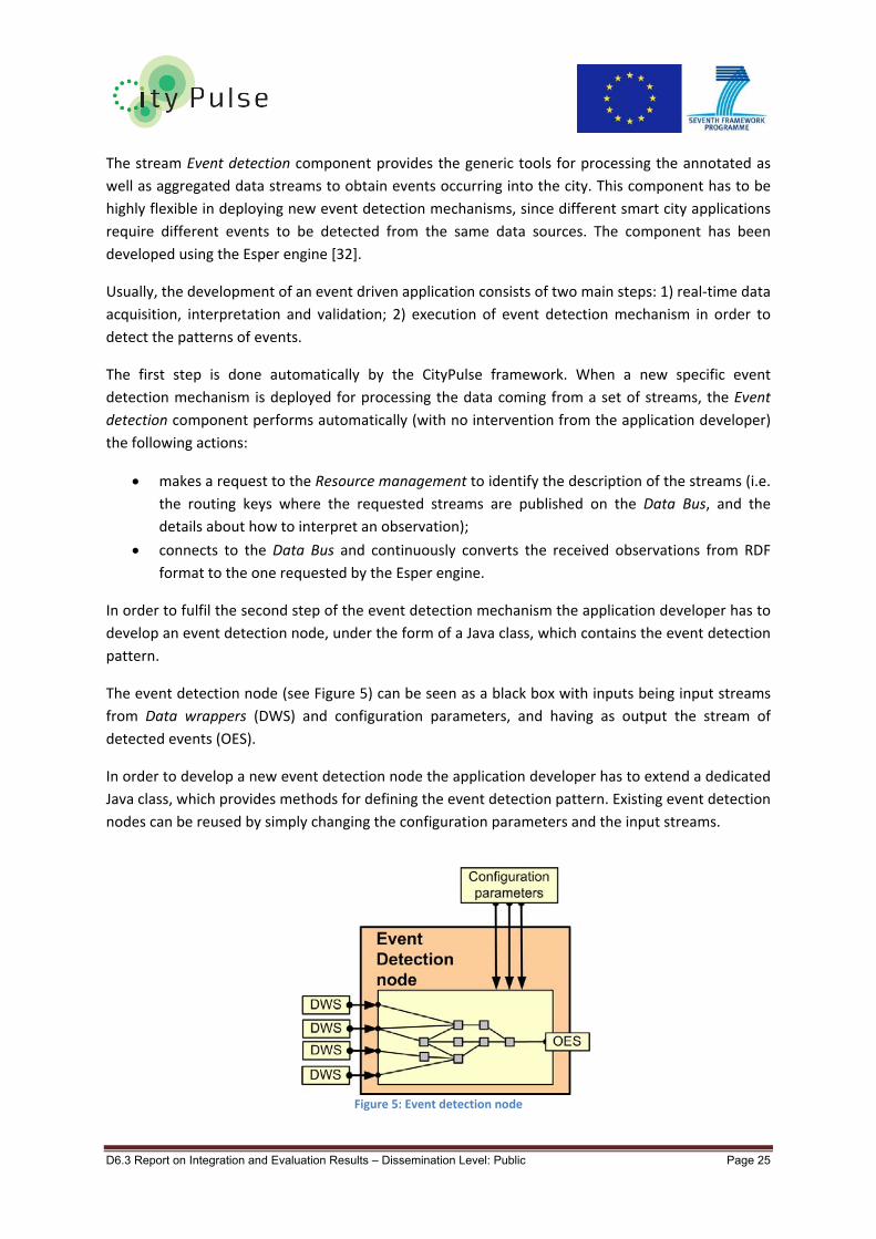
The stream Event detection component provides the generic tools for processing the annotated as
well as aggregated data streams to obtain events occurring into the city. This component has to be
highly flexible in deploying new event detection mechanisms, since different smart city applications
require different events to be detected from the same data sources. The component has been
developed using the Esper engine [32].
Usually, the development of an event driven application consists of two main steps: 1) real‐time data
acquisition, interpretation and validation; 2) execution of event detection mechanism in order to
detect the patterns of events.
The first step is done automatically by the CityPulse framework. When a new specific event
detection mechanism is deployed for processing the data coming from a set of streams, the Event
detection component performs automatically (with no intervention from the application developer)
the following actions:
makes a request to the Resource management to identify the description of the streams (i.e.
the routing keys where the requested streams are published on the Data Bus, and the
details about how to interpret an observation);
connects to the Data Bus and continuously converts the received observations from RDF
format to the one requested by the Esper engine.
In order to fulfil the second step of the event detection mechanism the application developer has to
develop an event detection node, under the form of a Java class, which contains the event detection
pattern.
The event detection node (see Figure 5) can be seen as a black box with inputs being input streams
from Data wrappers (DWS) and configuration parameters, and having as output the stream of
detected events (OES).
In order to develop a new event detection node the application developer has to extend a dedicated
Java class, which provides methods for defining the event detection pattern. Existing event detection
nodes can be reused by simply changing the configuration parameters and the input streams.
Figure 5: Event detection node

D6.3 Report on Integration and Evaluation Results – Dissemination Level: Public Page 26
The second module exposed by the Event detection component is used to process the Social Media
streams. The module analyses and annotates large‐scale real‐time Twitter data streams. A dedicated
Data wrapper is used to connect to the Twitter stream API and collect the data in the form of
tweets. The Data wrapper uses the Google‐translate API to automatically detect the source language
and translate the tweets to English to facilitate the Natural Language processing step. This in fact
enables the application developer to fetch data from any area (e.g. the area surrounding a certain
city).
The Social Media Event detection component reads a sequence of words in the sentence (tweet),
and passes it to a Natural Language Processing (NLP) unit (see Figure 6).
Figure 6: Social Media stream processing and event detection component
The processing unit is composed of three sub‐components: a Conditional Random Field Name Entity
Recognition [33], [34], a Convolutional Neural Network for deep learning for Part of Speech tagging,
and a multi‐view event extraction.
During the design time, the internal sub‐components are trained with a large corpus of Wikipedia
documents and historical Twitter data to guarantee a generalisable Natural Language Processing
model.
The Conditional Random Field Name Entity Recognition component assigns event tags to the words
in a Tweet given an event‐categories set ({TransportationEvent, EnvironmentalEvent, CulturalEvent,
SocialEvent, SportEvent, HealthEvent, CriminalEvent}), which is tailored for city related events. The
categories have been defined generic enough to cover future sub‐categorical event assignments (e.g
traffic and weather forecast events can be perceived as sub‐categories of TransportationEvent and
EnvironmentalEvent categories, respectively.) and they will be available to third‐party developers for
adoption and utilisation for new scenarios. Additionally, their respective event vocabularies are
adaptive and extendible to future events.
During the run time, the Conditional Random Field Name Entity Recognition component assigns
event tags to the words in a Tweet from the event categories set. Simultaneously, the trained
Convolutional Neural Network [35] component generates Part‐of‐Speech tags for atomic elements
of the Tweet. The obtained two views of the data (Conditional Random Field Name Entity
Recognition view and Convolutional Neural Network Part of Speech view) are then fed into a novel

D6.3 Report on Integration and Evaluation Results – Dissemination Level: Public Page 27
multi‐view event extraction component, where the obtained tags of the two views are mutually
validated and scored for a final sentence‐level inference. An example of sentence level inference is
in the case of tweets such as “seeing someone being given a parking ticket” where individual words
“parking” and “ticket” can belong to Transportation and Cultural events categories respectively
while considering the sentence grammar can clear up this confusion and assign the tweet to
Transportation category. The real‐time extracted city events are then used by Real‐time Adaptive
Urban Reasoning component to obtain a more comprehensive interpretation of the city events. The
extracted knowledge is utilised to complement the sensor stream information extraction and allows
obtaining of a more detailed interpretation of the city events when complementary citizen sensory
data can be extracted via social media processing.
2.2.1.6 QualitativeMonitoringThe CityPulse framework offers a two‐layered quality calculation mechanism to annotate data
streams with a Quality of Information (QoI) metric. The lower layer, called Atomic monitoring, is a
stream‐based quality calculation whereas the upper layer, Composite monitoring, combines different
data streams to include several sensor observations into QoI calculation. This enables applications
utilising the CityPulse framework to select the best fitting data streams for their needs. The current
implementation of the framework supports five QoI metrics: Age, Completeness, Correctness,
Frequency, and Latency.
To calculate this QoI metrics within the Atomic monitoring the domain expert has to specify a
SensorDescription within the Data wrapper (compare section III A). The fields, which are needed for
the QoI metrics are listed below:
1 sensordescription.maxLatency = 2 2 sensordescription.updateInterval = 60 3 sensordescription.fields = ["v1", "v2", “v3”] 4 sensordescription.field.v1.min = 0 5 sensordescription.field.v1.max = "@v3" 6 sensordescription.field.v1.dataType = "int" 7 sensordescription.field.v2.dataType = "datetime" 8 sensordescription.field.v2.format = "%Y-%m-%dT%H:%M:%S" 9 sensordescription.field.v3.dataType = “int” 10 …
Listing 1: Sensor Description
The first line states the maximum latency in seconds that should be met when the data wrapper
accesses new data. The following update interval specifies the time interval new observations can be
fetched (i.e. with pull connection) or the maximum time interval observations are published (i.e.
with push connection). The third line, namely “sensordescription.fields”, contains all features
contained in a single observation of the sensor stream. In this example the sensor stream consists of
three different features. v1 is a value of data type integer. The minimum value is 0. For the
maximum there is a special annotation with an @ followed by another fieldname. This states that
the maximum value is the current value in the same observation identified by the given fieldname.
v2 specifies a field containing a timestamp. The “format” parameter describes the format of the
incoming data fields. v3 is another value of data type integer. Other parameters for this field are
omitted in this example.

D6.3 Report on Integration and Evaluation Results – Dissemination Level: Public Page 28
Within the Atomic monitoring the values from the sensor description are compared to the current
observations delivered by the data stream. Based on the comparison and an internal rating
algorithm the QoI for the data stream is calculated.
To allow the domain expert to observe the quality of data streams, the CityPulse framework
provides a tool called QoI explorer to monitor deployed sensors in the city. Here, a map visualises
the state of each sensor (see Figure 7).
Figure 7: QoI Explorer
The tool shows an overview of all sensors within the city. The QoI of the streams is marked with
colours. There are different options to select specific QoI metrics or detailed views for individual
streams.
The Composite monitoring layer combines information from the Atomic monitoring components.
Based on entity, time and geospatial relationships, the different sources are evaluated and checked
for plausibility. Using the Composite monitoring, it is possible to detect faulty information sources
within a group of data sources by comparing to the other group members. Composite monitoring
compares acquired data with similar streams to determine correlations and looks for divergences.
When outliers of single data streams are detected, the Composite monitoring allows to search for
similar patterns in related data streams. Therefore, outliers can be separated from corrupted sensor
data.

D6.3 Report on Integration and Evaluation Results – Dissemination Level: Public Page 29
Figure 8 shows all the (four) phases of the process of Composite monitoring which calculates the
plausibility by utilising available overlapping information.
Figure 8: Composite Monitoring Process
During the first phase, spatially related streams are determined, which are able to support the
information of the event. In the second phase, the temporal distance is determined and used to
create a propagation model of the event. In the third step, correctness plausibility for each individual
correlated stream is calculated by comparing seasonally adjusted time series with the event. By
weighting the individual values with their spatio‐temporal distance, a combined composite
correctness value is calculated.
The Composite monitoring can be triggered by a set of events that will be compared against raw data
streams. The Domain Expert can improve the Composite monitoring by providing models that
determine the configuration for spatial distance model, temporal distance propagation and the
mapping between individual data stream types.
2.2.1.7 FaultRecoveryThe Fault recovery component ensures continuous and adequate operation of the CityPulse
application by generating estimated values for the data stream when the quality drops or it has
temporally missing observations. When the quality of the data stream is low for a longer time
period, an alternative data source has to be selected. The selection can be performed automatically
by the Technical adaptation component. In other words, the technical adaptation process does not
have to be triggered if the QoI of a stream is low only for a short period of time because the Fault
recovery component provides estimated values.
As presented in Figure 1, the Fault recovery component is integrated into the data wrapper. The
fault recovery mechanism is triggered to generate an estimated value when the atomic monitoring
component has determined that the current observation is invalid or missing.
The building blocks of the Fault recovery component are presented in Figure 9. The component has a
buffer which temporarily stores the latest observations generated by the data stream and a
reference dataset which contains sequences of valid consecutive observations from the data stream.
When an estimated value is requested, the k‐nearest neighbour algorithm [36] is used to select a
few sequences of observations from the references dataset, which are similar to the current
situation. At the end, the estimated value is computed from the selected sequences of observations.

D6.3 Report on Integration and Evaluation Results – Dissemination Level: Public Page 30
During normal operation, when the QoI of the stream is high, the fault recovery component extends
the reference data set with the sequences of observations from the buffer if a similar signal pattern
was not included before.
Initially, when the Data wrapper is deployed, the reference data set is empty and based on the
normal operation (from stream quality point of view) it is extended. As a result of that, the work of
the third‐party application developer is reduced, because he does not have to collect historical data
from the stream, to clean and to validate it in order to create the reference dataset. Using the API
exposed by the resource management, the third‐party application developer can turn on and off this
component based on the CityPulse application requirements.
Figure 9: Fault recovery component workflow.
2.2.1.8 Geo‐spatialdatabaseReasoning in cities depends heavily on the spatial context. For example, while temperature tends to
marginally vary across a neighbourhood, noise propagation depends on shielding buildings and
traffic flows on road networks, ongoing construction work, traffic density etc. Hence, spatial
reasoning requires appropriate distance measures. However, the integration of large amounts of
data sources requires efficient methods to provide the necessary information in (real) time. A
Geospatial Data Infrastructure is integrated to utilise infrastructure knowledge of the city. It enables
calculation of different distance measures and allows enhanced information interpolation to
increase reliability. Furthermore, an enhanced routing system enables multidimensional weighting
on path, e.g., depending on distance, duration, pollution, events or combined metrics. Thereby, it is
possible to avoid certain areas or block partial routes for specific applications (see Figure 10).
As an example, Figure 3 depicts classes of edges in the routable graph based on the weighted metric
for pollution. The geo‐spatial database can be used for developing CityPulse applications via a Java
API, which enables the following functionalities:
Calculate routes with:
o avoidance of areas,
o on a weighted street graph depending on priorities, e.g. pollution level,
o multiple alternative routes, which are sorted by a cost function;
Find sensors in an area or on a route;
Find events in an area or on a route;
Find objects like hospitals, waste‐bins, or further public infrastructure.

D6.3 Report on Integration and Evaluation Results – Dissemination Level: Public Page 31
Figure 10: Weighting Edges On a Street Graph (Green=Neutral, Yellow=Higher Cost, Red=Infinite Cost)
2.2.1.9 CityDashboardThe CityPulse framework provides immediate and intuitive visual access to the results of its
intelligent processing and manipulation of data and events. The ability to record and store historical
(cleaned and summarised) data for post‐processing makes it possible to analyse the status of the city
not only on the go but also at any point in time, enabling diagnosing and “post mortem” analysis of
any incidents or relevant situation that might have occurred. To facilitate that, a dashboard for
visualising the dynamic data of the smart cities is provided on top of the CityPulse framework. Based
on this dashboard, the user has the possibility to visualise a holistic and summarised view of data
across multiple contexts or a detailed view of data of interest, as well as to monitor the city life as it
evolves and as things happen. The investigation of past city events or incidents can be conducted
from different perspectives, e.g. by observing the correlations between various streams, since the
streaming data is stored in the framework for a period of time which can be configured, and it can
be retrieved for visualisation and analysis at any moment. Figure 11 depicts a snapshot of the
CityPulse dashboard application.
In order to display the status of the city, the dashboard application connects directly to the resource
management or to the data bus for fetching the description of the available streams or the real‐
time/historical observations. The dashboard application can be used out of the box and there are no
configuration or development steps that have to be done by the application developer.

D6.3 Report on Integration and Evaluation Results – Dissemination Level: Public Page 32
Figure 11: CityPulse dashboard application
2.2.2 Real‐timeAdaptiveUrbanReasoningSmart city applications in changing environments require to take into account user preferences and
requirements, as well as dynamic contextual information represented by real‐time events, in order
to provide optimal decision support to the end user at any time.
The event‐driven adaptation and context‐driven user‐centricity of the CityPulse framework are
materialized by a close loop between the Contextual Filtering component, the user application, and
the Decision support component as illustrated in Figure 12.
Figure 12: Event‐based User‐Centric Decision Support
The user‐centric and event‐driven reasoning capabilities of the framework strongly rely on the tight
interaction between the user application and the Contextual Filtering component respectively, with
the former being in charge of the bidirectional communication with the other two. The user
application is also tightly connected with the Decision support component in requesting to compute
answers to a decision problem by reflecting constraints and preferences specified by the user
himself.

D6.3 Report on Integration and Evaluation Results – Dissemination Level: Public Page 33
This user‐driven loop between the Contextual Filtering and the Decision support component makes it
easier for application developers to decide whether to give complete control to the end user on
when and how to request adaptation after critical events have been detected, or automatically
suggest new solutions.
In the remainder of this section we provide details of both the Contextual Filtering and the Decision
support components for real‐time adaptive urban reasoning.
2.2.2.1 ContextualFilteringThe main role of the Contextual Filtering component is to continuously identify and filter events that
might affect the optimal result of the decision making task (performed by the Decision support
component), and react to such changes in the real world by requesting the Decision support for the
computation of a new solution when needed. This not only ensures that the selected solution
provided to the user remains the best option when situations change, but it also empowers the
CityPulse framework to automatically provide alternative decisions whenever the selected best
decision is no longer the best for a particular situation.
The adaptive capability of identifying and reacting to unexpected events in a user‐centric way relies
on two aspects: i) a characterisation of the user’s implicit and explicit context provided by the user
application (including user requirements, preferences, events of interests and activities), and ii) a
stream of events provided by the Event detection component.
The filtering capability of the Contextual Filtering component is key not only for context‐awareness,
but also for scalability. In fact, the Contextual Filtering component only subscribes to a subset of
events among those provided by the Event detection component. The type of events the Contextual
Filtering subscribes to are application‐specific and are in part dependent on the domain (determined
at design‐time), and in part contextualized, depending on the specific reasoning task or user
preferences specified by the user application (determined at run‐time). For example, in the Travel
Planner application (see section IV), traffic and weather conditions are relevant types of events that
can be characterised at design time. However, when the user application provides a solution to go
from a starting point A to an ending point B, only traffic and weather conditions in areas around that
specific path are potentially relevant, and they can be augmented by the user interest in other types
of events on the way (such as cultural or social gathering).
The occurrence of such relevant events is notified to the Contextual Filtering component by the
Event detection component, which provides additional metadata describing the event. Listing 2
illustrates an example of an annotated event about a traffic jam, as it is received by the Contextual
Filtering component. Information about the user context can be gathered by the Contextual Filtering
in several ways: it can be either explicitly stated in the event request or in the user application (e.g.
specifying events of interest), or it can be explicitly or implicitly acquired by identifying user’s current
activity (e.g. using the speed to detect that the user is in a car, or having the user specifying in the
application what type of transportation he/she is using). With this information, the Contextual
Filtering component is able to: i) select, among the list of detected filtered events, the ones that are
contextually relevant, and ii) continuously rank their level of criticality to decide when an action is to
be triggered.

D6.3 Report on Integration and Evaluation Results – Dissemination Level: Public Page 34
@prefix geo:http://www.w3.org/2003/01/geo/wgs84_pos# . @prefix sao: <http://purl.oclc.org/NET/UNIS/sao/sao#> . @prefix tl: <http://purl.org/NET/c4dm/timeline.owl#> . @prefix xsd: <http://www.w3.org/2001/XMLSchema#> . @prefix prov: <http://www.w3.org/ns/prov#> . @prefix ec: <http://purl.oclc.org/NET/UNIS/sao/ec#> . sao:c2d69ca8-b404-4006-ad48-9317397251ab a ec:TrafficJam ; ec:hasSource "SENSOR" ; sao:hasLevel "1"^^xsd:long ; sao:hasLocation [ a geo:Instant ; geo:lat "56.17091325696965"^^xsd:double ; geo:lon "10.15728564169882"^^xsd:double ] ; sao:hasType ec:TransportationEvent ; tl:time "2015-11-26T13:27:46.079Z"^^xsd:dateTime .
Listing 2: An example of an annotated event
The level of criticality of events is dynamically assessed by the Contextual Filtering component based
on metrics such as the distance between a detected event and user’s current location, or an explicit
measure of how severe the event is (referred to as Event Level). The current implementation of the
Contextual Filtering component uses a linear combination of these metrics. An application developer
can configure such metrics and users can modify them in order to satisfy their own requirements. In
terms of implementation, the Contextual Filtering component is encoded as logical rules. The
underlying logic used to implement the Contextual Filtering component is based on the Stable Model
Semantics of Answer Set Programming (ASP) [37] and relies on the efficient implementation of such
semantics in the Clingo engine [38]. The ability of ASP to support common‐sense and default
reasoning makes it possible to activate and deactivate certain rules when a combination of
unexpected changes in the real world affect each other.
Listing 3 is an extract of the logic rules used in the Contextual Filtering component. Rule 1 filters out
unrelated events. Rule 2 generates sets of solutions containing one critical event each per solution,
provided that the event is not15 expired. Rules 3‐7 compute the criticality of an event. Based on this
level of criticality, the Contextual Filtering refers back to the user application that an action is
required, which can be either generating a new request for the Decision support component to
automatically provide an alternative (better) solution, or informing the user about the critical event
let the user decide whether a new solution is needed. The fully declarative nature of ASP facilitates
automatic generation of such rules for application developers, starting from high‐level specification
of what events are relevant for the application and how the ranking metrics are formally defined.
This is a crucial advantage for customizing the Contextual Filtering component to application‐
dependent behaviour.
Context‐awareness has been long studied in the domain of service provision and mobile computing,
as the ability of an application to “automatically adapt to the discovered context (environmental
situations or conditions) by changing the application behaviour according to the latest context” [39],
but scalable solutions to do that in dynamic settings and going beyond complex event detection
towards non‐monotonic reasoning is still under investigation [40], [41].
15 Note that we use default negation here, a powerful way of reasoning by default that is typical of non‐monotonic approaches such as those based on ASP.

D6.3 Report on Integration and Evaluation Results – Dissemination Level: Public Page 35
(r1) related_city_event(Id) :- filtering_event(Category), city_event(Id, Category, Source). (r2) 1 <= {selected_city_event(EventId) : related_city_event(EventId), not expired_event(EventId)} <= 1. (r3) value(RankEleName,Value):- selected_city_event(EventId), ranking_city_event_data(EventId, RankEleName,Value). (r4) value_with_ranking_type(RankingElementName, M):- value(RankingElementName,Value), ranking_multiplier(RankingElementName,Int), M = Value*Int. (r5) sum(C) : value_with_ranking_type("EVENT_LEVEL",Value1), value_with_ranking_type("DISTANCE",Value2), C = Value1+Value2. (r6) criticality(C) :- C = M/100, sum(M). (r7) critical_city_event(EventId,C):- selected_city_event(EventId), criticality(C).
Listing 3: Logic rules for contextual filtering of events with ranking through linear combination
The main novelty of this approach used by the Contextual Filtering component for adaptive and
context‐aware reasoning in dynamic environments is the ability to use such complex reasoning
capabilities to efficiently and dynamically select only relevant information to tackle the challenge of
converting data into knowledge in dynamic environments in a scalable way.
2.2.2.2 Event‐basedUser‐CentricDecisionSupportThe Decision support component of the CityPulse framework represents higher‐level intelligence,
and the main role of this component is to enable reactive decision support functionalities to be
easily deployed, providing the most suitable answers at the right time.
The reasoning capabilities needed to support users in making better decisions require handling
incomplete, diverse and unreliable input, as well as constraints and preferences in the deduction
process. This expressivity in the Decision support component is achieved by using a declarative non‐
monotonic logic reasoning approach based on Answer Set Programming. Semantic technologies for
handling data streams, in fact, cannot exhibit complex reasoning capabilities such as the ability of
managing defaults, common‐sense, preferences, recursion, and non‐determinism. Conversely, state‐
of‐the‐art logic‐based non‐monotonic reasoners can perform such tasks but are only suitable for
data that changes in low volumes at low frequency. Therefore, the main challenge addressed by the
Decision support component is to enable expressive reasoning for decision support in a scalable way.
In our approach we combine the advantages of semantic query processing and non‐monotonic
reasoning based on the general idea behind StreamRule [42]. We have identified features that can
affect scalability of such a combined approach and we have exploited the user‐centric features and
adaptive filtering of relevant events to reduce the input size and therefore the search space for the
decision support task, thus increasing the potential for better scalability. As mentioned earlier in this
paper, the user‐centric and event‐driven features of the Decision support component strongly rely
on the tight interaction with the user application and the Contextual Filtering component
respectively, with the former being in charge of the bidirectional communication with the other two,
as represented in Figure 12.
In what follows, we detail the input and output used by the Decision support component, and also
introduce the main reasoning modules that are currently implemented as part of the CityPulse
framework. The input for the Decision support component is illustrated in Figure 13.

D6.3 Report on Integration and Evaluation Results – Dissemination Level: Public Page 36
Figure 13: Decision Support I/O
A Reasoning request consists of:
User Reference: uniquely identifies the user that made the request. Such reference is related
to user credentials that will be used in the final integration activities in order to manage user
logins and instances of the CityPulse framework in different cities.
Type: indicates the reasoning task required by the application. This is used directly by the
Decision support component to select which set of rules to apply, and needs to be identified
among a set of available options at design time by the application developer.
Functional Details: represent the qualitative criteria used in the reasoning task to produce a
solution that best fits the user needs.
The Functional details are composed by:
Functional Parameters, defining mandatory information for the Reasoning Request (such as
start and end location in a travel planner scenario);
Functional Constraints, defining a numerical threshold for specific functional aspects of the
Reasoning Request (such as cost of a trip, distance or travel time in a travel planner
scenario). These restrictions are evaluated as hard constraints, which needs to be fulfilled by
each of the alternative solutions offered to the user;
Functional Preferences, which encode two types of soft constraints: a qualitative
optimisation statement defined on the same functional aspects used in the Functional
Constraint (such as minimisation of the travel time); or a qualitative partial order over such
optimization statements (such as preference on the minimisation of the distance over
minimization of the travel time). Preferences are used by the Decision support component
to provide to the user the optimal solution among those verifying the functional constraints.
Given the fully declarative approach of ASP, we are able to provide a specification of all aspects of a
Reasoning Request, which can be automatically mapped into logic rules. As a result, we achieve a
high degree of flexibility to adapt to new scenarios and requirements, which makes it easier for
developers to build new applications. In the reasoning process performed by the Decision support
component, declarative rules derived from the Reasoning Request are combined in a single logic ASP
program with the following input:

D6.3 Report on Integration and Evaluation Results – Dissemination Level: Public Page 37
Sub‐Answers from external modules. These are facts computed by external models as
subtasks of the decision support problem. Calls to such external modules can be used to
improve scalability by reducing the solution space, or for privacy reasons. For example, in a
travel planner scenario, a reduced list of all possible routes to go from A to B within a
geographical area is provided by the Geospatial Data Infrastructure component. This does
not imply any contextual reasoning, qualitative optimization, or event‐driven adaptation,
which is instead provided by the Decision support component.
Background Knowledge. This is static information about a particular domain (such as the
location of parking areas).
Events Snapshot. This information comes from the Data federation component, and consists
of the latest values of related events in the city (such as traffic levels in particular areas).
Events snapshots are used the first time a solution is computed and ensure this solution is
based on the most updated values. Dynamic changes to these values are then continuously
detected and used by the Decision support component via the adaptive filtering mechanism
of the Contextual Filtering component.
The Decision support component produces a set of answers to the Reasoning Request that satisfy all
user’s requirements and preferences in the best possible way. These solutions are computed by
applying sets of rules deployed as scenario‐driven decision support modules. We currently support
three different types of decision support modules, covering a broad range of application scenarios:
Routing Module. It provides the best solution(s) for a routing task, which is continuously
updated based on incoming events and their criticality; the travel planner scenario relies on
this module, and so do other scenarios where finding the optimal route is the main task, but
the selection criteria (including constraints and preferences) might vary. Examples include
the ability to schedule optimal pick‐up for health services, green bike tours and alike.
Optimal Selection Module. It provides the best selection among a set of alternative based on
optimisation criteria, constraints and preferences; the parking scenario is part of this
category.
Planning Module. It provides optimal solutions to a planning problem, and continuously
updates the options when the selected one is no longer feasible (based on Functional
Constraints) or is no longer optimal (based on Functional Preferences); scenarios that are
part of the cultural sector (such as planning activities in the city based on user interests or
schedule) or the energy sector (such as planning household usage based on user‐defined
constraints and cost) are candidate scenarios for using this module.
These modules are available as API to be used by application developers in a broad range of
applications. Since decision support tasks are strongly domain‐dependent, different type of
reasoning tasks would require additional Decision Support modules to be developed. The CityPulse
framework provides a set of guidelines for developing new decision support modules, which requires
knowledge of Answer Set Programming to develop the proper application logic.

D6.3 Report on Integration and Evaluation Results – Dissemination Level: Public Page 38
2.2.2.3 TechnicalAdaptationThe CityPulse framework leverages the Technical adaptation component to automatically detect
critical quality updates for the federated data streams used in the Data federation component and
make adjustments. IoT streams are inherently dynamic in nature and often unreliable, hence more
prone of getting fluctuations in the quality metrics. Therefore, it is utmost necessary to have a
quality‐aware adaptation mechanism for IoT streams. Using the Technical adaptation component,
the quality of user queries deployed by the Data federation component can be maintained
automatically by dynamically replacing data sources, unlike existing adaptive CEP systems which
leverage query‐rewriting and re‐ordering of the query operators.
The CityPulse framework facilitates adaptability in quality‐aware federation of IoT streams for smart
city applications. In order to provide technical adaptation to increase robustness of smart city
applications, the following three steps are involved:
1. Monitoring Quality Updates: to monitor any updates in the quality metrics of the IoT
streams involved in stream federation;
2. Evaluate Criticality: to determine whether any particular quality update is critical and if there
is any adaptation action that should be carried out based on the composition plan and non‐
functional requirements; and
3. Adaptation Handling: when adaptation is triggered, determine the adaptation scope (i.e.,
part of the composition plan (produced by the Data federation component) that needs to be
changed), make an adaptation request to the data federation and recompose the adaptation
scope and redeploy the newly derived composition plan.
Figure 14 illustrates the process and the components used to achieve adaptability in stream
federation following the above mentioned three steps.
Figure 14: Adaptability in Stream Federation
During the event streams discovery and composition process, numerical quality vectors can be used
to specify constraints over the quality metrics for data streams. For example, if we consider some
typical quality attributes, including latency, price, energy consumption, bandwidth consumption,
availability, completeness, accuracy and security, a numerical quality vector:

D6.3 Report on Integration and Evaluation Results – Dissemination Level: Public Page 39
Q=<L,P,E,B,Ava,C,Acc,S>
can be used to specify the quality of a data stream w.r.t. these dimensions along with the static data
stream description. Similarly, a quality constraint vector Q’ can be used to specify the quality
constraints as thresholds for the quality metrics in the stream discovery or composition requests. If
none of the quality values in Q breaks the threshold in Q’, the data stream is considered to be a
candidate for the discovery and composition. A weight vector:
W=<Lw,Pw,Ew,Bw,Avaw,Cw,Accw,Sw>
contains 0 to 1 weights for each quality metrics within the requests, representing the preferences
over quality metrics. The weight vector is used to normalize the quality vectors for all candidates
based on simple additive weighting, the results are ranked and the top candidate is chosen. During
runtime, the quality vectors will be re‐computed based on most recent quality value updates, and
the constraints are re‐evaluated to determine if the quality of the data stream still satisfies the
constraints. If optimal candidates must be used for the application domain at all times, updated
quality vectors are also re‐ranked, and the new top candidate is chosen to be the adaptation result.
It is worth mentioning that such preferences and requirements are specified as a default
configuration within a specific application, and they can be overwritten by user specific settings.
The Technical adaptation component is closely integrated with the Data federation component. It
receives quality updates disseminated in the Data Bus. The quality updates are originally produced
by the Quality Monitoring component. The Technical adaptation component is transparent to the
end user as long as the adaptations are successful. Otherwise, it may produce a failure notification
to the application interface. The adaptation strategies of the Technical adaptation component can
be configured by a third‐party developer by changing the AdaptationMode parameter in the API
offered by the Data federation component. Then, an initialization API is invoked at the backend
system to create an AdaptationManager instance for the specific request.
2.2.3 ComponentsinterdependenciesThe CityPulse components are highly flexible, which allows multiple configurations of exploitation. In
other words, the application developer can deploy only a subset of the components based on the
requirements of the application which have to be developed.
There are interdependencies among the components of the framework and it is possible that the
application developer will have to deploy also other CityPulse components in order to have a certain
feature running.
Considering the out of the box installation, when the application developer simply deploys and
configures a component, he has to deploy also the CityPulse components which are below the
considered component in the architecture. For other types of installations the application developer
can replace one or several components with its own custom‐made modules. This is possible because
the components are using REST and AMQP protocols to communicate.
2.2.4 Context‐AwareRealTimeTravelPlannerIn order to demonstrate how the CityPulse framework can be used to develop applications for smart
cities and citizens, we have implemented a context‐aware real time Travel Planner using the live

D6.3 Report on Integration and Evaluation Results – Dissemination Level: Public Page 40
data from the city of Aarhus, Denmark. The scenario was defined in collaboration with the IT
departments of Aarhus municipality and the following criteria have been considered: the impact of
the application for the citizens and the data availability. The selected scenario belongs to the traffic
domain, but as it was presented earlier in this paper, the CityPulse framework is generic and can be
applied in any domain.
This scenario aims to provide a travel planning solutions that goes beyond the state of the art
solutions by allowing users to provide multi‐dimensional requirements and preferences such as air
quality, traffic conditions and parking availability. In this way the users receive parking and route
recommendations based on the current context of the city. In addition to this, Travel Planner
continuously monitors the user context and events detected on the planned route. User will be
prompted to opt for a detour if the real time conditions on the planned journey do not meet the
user specified criteria anymore.
In this case, the application developer has performed the following activities:
Configured the CityPulse framework components;
Deployed the components into a back end server;
Developed a smart phone application using the APIs exposed by the framework in order to
respond to the user requests. This application does not perform any data processing.
For this application, and very probably for most of the CityPulse enabled applications, the
framework components can be divided into two different categories. First of all, the large‐scale data
stream processing modules are configured and deployed in order to permanently monitor the status
of Aarhus city. In this way, when a new user logs into the mobile application and generates a request
for a recommendation, the back‐end application can provide the answer based on the current traffic
or pollution situation in the city.
The second category of components, which perform real‐time adaptive urban reasoning, are
triggered when the user requests the routing or parking recommendation.
The following subsections present the specific workflows for the two categories of components
mentioned above. For each particular workflow, the activities that have to be performed by the
application developer at design time are marked at the beginning.
2.2.4.1 Large‐scaledatastreamprocessingworkflowFor the considered scenario, the large‐scale data stream processing modules are configured to
process in real time the parking and traffic data coming from the city sensors with the scope of
detecting relevant events for the users traveling in the city. Figure 15 depicts the workflow and this
subsection is dedicated to explaining the activities.

D6.3 Report on Integration and Evaluation Results – Dissemination Level: Public Page 41
Figure 15. Large‐scale data stream processing workflow.
For the realization of the envisaged Travel Planner application, the required data streams must be
made available within the framework at first in the design phase. For this, corresponding Data
wrappers for both data streams need to be developed. The Aarhus Traffic wrapper was realised by
implementing an HTTP Pull Connection (i.e. HTTP client) extending the abstract Sensor Connection. It
fetches new sensor readings from the ODAA portal. The response messages are JSON encoded
documents. Consequently, a JSON Parser was implemented to extract the relevant information from
these messages, namely the number of vehicles passing the two measurement points
(“vehicleCount”) and their average speed (“avgSpeed”).
The second Data wrapper implemented fetches the parking data of parking garages in Aarhus.
Similar to the traffic data stream, the Aarhus Parking data is provided by the ODAA platform and
encoded as JSON message. Therefore, the same HTTP Pull Connection but a different JSON Parser is
used. The stream provides information about the total number of parking spaces in the garage
(“totalSpace”) and the number of occupied spaces/vehicles in the garage (“vehicleCount”).
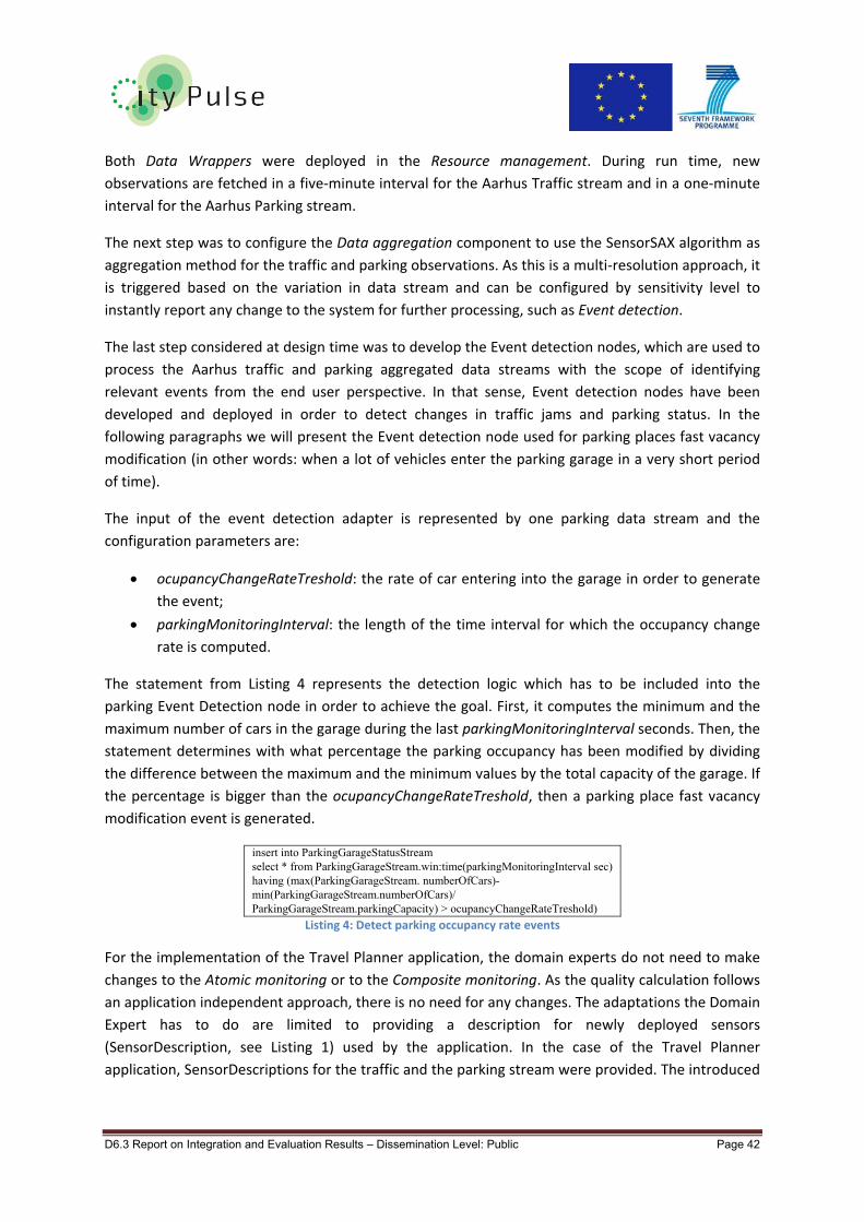
D6.3 Report on Integration and Evaluation Results – Dissemination Level: Public Page 42
Both Data Wrappers were deployed in the Resource management. During run time, new
observations are fetched in a five‐minute interval for the Aarhus Traffic stream and in a one‐minute
interval for the Aarhus Parking stream.
The next step was to configure the Data aggregation component to use the SensorSAX algorithm as
aggregation method for the traffic and parking observations. As this is a multi‐resolution approach, it
is triggered based on the variation in data stream and can be configured by sensitivity level to
instantly report any change to the system for further processing, such as Event detection.
The last step considered at design time was to develop the Event detection nodes, which are used to
process the Aarhus traffic and parking aggregated data streams with the scope of identifying
relevant events from the end user perspective. In that sense, Event detection nodes have been
developed and deployed in order to detect changes in traffic jams and parking status. In the
following paragraphs we will present the Event detection node used for parking places fast vacancy
modification (in other words: when a lot of vehicles enter the parking garage in a very short period
of time).
The input of the event detection adapter is represented by one parking data stream and the
configuration parameters are:
ocupancyChangeRateTreshold: the rate of car entering into the garage in order to generate
the event;
parkingMonitoringInterval: the length of the time interval for which the occupancy change
rate is computed.
The statement from Listing 4 represents the detection logic which has to be included into the
parking Event Detection node in order to achieve the goal. First, it computes the minimum and the
maximum number of cars in the garage during the last parkingMonitoringInterval seconds. Then, the
statement determines with what percentage the parking occupancy has been modified by dividing
the difference between the maximum and the minimum values by the total capacity of the garage. If
the percentage is bigger than the ocupancyChangeRateTreshold, then a parking place fast vacancy
modification event is generated.
insert into ParkingGarageStatusStream select * from ParkingGarageStream.win:time(parkingMonitoringInterval sec) having (max(ParkingGarageStream. numberOfCars)-min(ParkingGarageStream.numberOfCars)/ ParkingGarageStream.parkingCapacity) > ocupancyChangeRateTreshold)
Listing 4: Detect parking occupancy rate events
For the implementation of the Travel Planner application, the domain experts do not need to make
changes to the Atomic monitoring or to the Composite monitoring. As the quality calculation follows
an application independent approach, there is no need for any changes. The adaptations the Domain
Expert has to do are limited to providing a description for newly deployed sensors
(SensorDescription, see Listing 1) used by the application. In the case of the Travel Planner
application, SensorDescriptions for the traffic and the parking stream were provided. The introduced

D6.3 Report on Integration and Evaluation Results – Dissemination Level: Public Page 43
QoI Explorer enables the application developer to check the quality of sensors along a selected route
and to check the results for plausibility.
At run time, after the CityPulse components have been deployed, the Data wrappers start to fetch
observations from the Aarhus city data streams. When an observation is received, the atomic
monitoring is performed and the QoI description of the stream is updated. If the observation is
missing or the quality of the stream is low, the Fault recovery component is triggered to generate an
estimation.
The observations along with the QoI determined in the Atomic monitoring is annotated semantically
afterwards. The annotation process is generic and uses the details provided in the
SensorDescription, where required information such as the general domain of the stream, the
nature/concept of an observation and the unit of measurement for the observation are specified.
Next, the numeric values of the observation are aggregated accordingly using the selected
algorithm. Figure 16 depicts the data captured for average speed via the corresponding sensor
points and illustrates SensorSAX patterns created from the raw data.
Figure 16. Data aggregation using SensorSAX with minimum window size is 1 and sensitivity level is 0.3 for average speed observation of Aarhus traffic data stream.
At the end, the aggregated streams of observations are processed by the Event detection component
in order to extract the parking and traffic events. Once an event is detected, it is published on the
Data Bus to be further used by the Decision support and Contextual Filtering components and a
notification is sent to the Geospatial Data Infrastructure. In this way, the process of computing the
routes (see the Geospatial Data Infrastructure APIs is influences by the current city context.
2.2.4.2 Real‐timeAdaptiveUrbanReasoningforTravelPlannerFor the considered scenario, the real time adaptive urban reasoning components are used to provide
answers when a user generates routes and parking recommendation requests. Figure 17 depicts the
workflow executed by the components for providing an answer when a route recommendation is
requested.

D6.3 Report on Integration and Evaluation Results – Dissemination Level: Public Page 44
As mentioned above, all the CityPulse framework components are deployed on a back‐end server
and are accessible via a set of APIs. As a result, the application developer has only to develop a user‐
friendly front‐end application that calls the framework APIs. In our case we have developed an
Android application.
Figure 18 depicts the user interfaces used by the end user to set the travel preferences and the
destination point.
Figure 17. Real‐time Adaptive Urban Reasoning workflow for Travel Planner.

D6.3 Report on Integration and Evaluation Results – Dissemination Level: Public Page 45
Figure 18 The user interfaces of the Android application used to select the starting point and the travel preferences.
After the user has filled in the details and made the request using the user interface, the mobile
application generates the appropriate request for the Decision support component which has the
following main fields:
Type: indicating what decision support module is to be used for this application (“TRAVEL‐
PLANNER” in this case);
Functional details: specifying possible values of user’s requirements, including:
o Functional parameters: mandatory information that the user provides such as
starting and ending locations, starting date and time, and transportation type (car,
bicycle, or walk).
o Functional constraints: numerical thresholds for cost of a trip, distance, or travel
time.
o Functional preferences: the user can specify his preferences along selected routes,
which hold the functional constraints. These preferences can be the minimization or
the maximisation of travel time or distance.
The functional constraints and preferences specify different thresholds and minimisation criteria for
electing the route. During the development of the mobile application, the domain expert has
computed a default set of values for these thresholds. As a result, the route constraints user
interface from the figure above allows the user to select between the fastest/shortest routes. If
needed, more fields can be added in this user interface in order to allow more fine‐grained
constraints specifications, but the usability of the application may suffer.

D6.3 Report on Integration and Evaluation Results – Dissemination Level: Public Page 46
This concrete reasoning request is automatically mapped into ASP rules (see example rules 4‐7 in
Listing 5), and combined with the specific scenario‐driven rules for the Travel Planner Decision
Support module16. The Decision support component collects all possible routes from the Geo‐spatial
database infrastructure as well as the last snapshot of values of relevant functional properties for
those routes which can be produced dynamically by the Data federation component or retrieved
from the Knowledge base (rules 1‐3).
1. input_get_routes(SP, EP, V, 5) :‐
parameter("STARTING_POINT", SP),
parameter("ENDING_POINT", EP), route_costMode(V).
2. route(@get_routes(SP, EP, V, N)) :‐ input_get_routes(SP, EP, V, N).
3. route_data(@get_routes_data(SP, EP, V, N)) :‐
input_get_routes(SP, EP, V, N).
4. parameter("STARTING_POINT","10.116919 56.226144").
5. parameter("ENDING_POINT","10.1591864 56.1481156").
6. minimize{AV@2 ∶ valueOf("DISTANCE", AV)}.
7. minimize{AV@1 ∶ valueOf("TRAVEL_TIME ", AV)}.
Listing 5 – A snapshot of logic decision support rules for the Travel Planner scenario
Afterwards the Decision support component relies on the Clingo4 ASP reasoner to compute the
optimal routes that best satisfy the user’s reasoning request. In the current implementation of the
Decision support, the user will receive at most 5 optimal routes.
Figure 19 depicts the user interface where the routes computed by the Decision support are
displayed to the end user.
Figure 19 The user interfaces of the Android application: a) select the preferred route; b) notification of a traffic jam which appeared on the selected route while the user is travelling.
16 Note that this can be fully automated due to the declarative nature of our approach to rule‐based reasoning based on ASP.

D6.3 Report on Integration and Evaluation Results – Dissemination Level: Public Page 47
After the user selects the preferred route, a request is generated to the Contextual filtering
component in order to identify the relevant events for the use while he/she is traveling. The request
includes the following properties:
Route of interest: the current route of the user.
Filtering Factors: used to filter unrelated (unwanted) events out, and include event’s source,
event’s category, and user’s activity, as specified in a user‐context ontology17. For this
particular scenario, the activities included in our ontology include CarCommute (user is
traveling by car), or Walk, or BikeCommute (user is traveling by bike).
Ranking Factor: identifies which metric is preferred by the user for ranking the criticality of
incoming events. We have currently implemented the Ranking Factor based on two metrics:
distance, and gravity of the event. In order to combine these two metrics, we use the linear
combination approach, where the user can identify weights (or importance) for each metric.
Similar to the decision support constraints and preferences, the filtering and ranking factors are
selected by the domain expert during the mobile application development stage, but they can be
made accessible to the end users.
Once the user has selected one of the routes computed by the Decision support component, the
Contextual Filtering component sends a request to the Geospatial Database Infrastructure
component to obtain the description of the event streams available on the selected route, as
registered at design time by the Event detection component. The Contextual Filtering component
uses these descriptions to subscribe to detected events via a Data Bus. In addition, the Contextual
Filtering also receives the contextual information of the user (currently including location) from the
user/application as a stream. Whenever there is a new event detected by the Event detection
component, the Contextual Filtering component filters and assigns the most appropriate criticality (0
if not critical, from 1 to 5 if it is critical) to the new event. If the new event is marked as critical18, the
user receives a notification and he/she has the option to change the current solution and request a
new one or ignore the event. Figure 19 depicts the notification received by the end user, while s/he
is traveling and a traffic event is detected on his/hers route.
In addition to the contextual filtering request, the mobile application triggers the Data federation to
continuously compute the average speed of the cars from the selected route. At design time, the
application developer has configured the Data federation component to store the meta‐data for the
traffic sensors and to use the "EL" load balancing strategy (starts with one engine instance and
creates more instances elastically when all existing instances have reached maximum capacity).
The request generated by the mobile application contains the following fields:
ep: the query pattern, in this application it is a conjunction of primitive traffic report events,
constraint: the QoS constraint vector, absence of the constraint results in application of a set of defaulted loose constraints,
17 Note that the ontology can be extended by adding new activities. 18 Note that we currently provide all events marked with criticality higher than 0, but this can be changed by setting a different threshold or limiting the notification to the top‐k events.

D6.3 Report on Integration and Evaluation Results – Dissemination Level: Public Page 48
weight: the QoS weight vector, absence of the weights results in equal weights configured to all QoS metrics,
continuous: true has been selected to compute the average continuously;
engineType: type of RDF processing engine to be used; can be 'CQELS' or 'CSPARQL'
aggOp: aggregation operator, which for our particular situation is average. The ep in the request contains the functional requirements for the primitive traffic data streams, e.g.
what properties should they measure and what are the locations of the sensors (computed from the
route selected by the user). Combining the functional requirements with the QoS constraints and
preferences, the Data federation component creates the optimal composition plan for the request
based on the stream meta‐data provided in the knowledge base.
According to the engineType parameter specified in the request, the composition plan is
transformed into a CQELS or CSPARQL query, as shown in Listing 6. A post‐processing is applied to
the query evaluation results to aggregate the observation values, using the aggregation operator
specified in the aggOp. If the aggOp is set to empty, then no post‐processing is invoked.
@prefix sao: <http://purl.oclc.org/NET/UNIS/sao/sao#>. @prefix ssn: <http://purl.oclc.org/NET/ssnx/ssn#>. @prefix owls: <http://www.daml.org/services/owl-s/1.2/Service.owl#>. @prefix ct: <http://ict-citypulse.eu/city#>. SELECT ?obId1 ?obId2 ?v1 ?v2 WHERE { ?p1 a ct:AverageSpeed. ?p2 a ct:AverageSpeed. STREAM <Traffic226> [range 3s ] {?obId1 a ?ob. ?obId1 ssn:observedProperty ?p1. ?obId1 sao:value ?v1.} STREAM <Traffic439> [range 3s ] {?obId2 a ?ob. ?obId2 ssn:observedProperty ?p2. ?obId2 sao:value ?v2.} }
Data Federation is a generic component that gives continuous query results over federated data
streams. Since it follows a service‐oriented approach, the discovery and composition algorithms do
not require changes based on specific application domains, as long as the service description model
is used by the service providers and consumers.
The domain experts can choose between different default target continuous query evaluation
systems (currently CQELS and C‐SPARQL are integrated), based on the different characteristics of the
application domains, e.g., the average query size, the frequency of data streams and the size of the
background knowledge. These factors may affect the performance of the target systems (for more
information refer to [43]) and a configuration based on specific scenarios could be beneficial but is
not mandatory.
Listing 6: Sample CQELS Query Generated from Composition Plan

D6.3 Report on Integration and Evaluation Results – Dissemination Level: Public Page 49
3 Performance Evaluation
3.1 KPIsIn the following sections, a summary of the selected KPIs form D.2.1 are presented. The selected
KPIs are used for the evaluation of the performance of the different CityPulse components.
3.1.1 ObservationPointKPIsTable 3: Observation Point Key Performance Indicators (KPIs)
KPI Name Description ‐ What this KPI is about
Metric ‐ What is measured in the KPI
Method ‐ Practical way to measure KPI
Frequency Number of observations recorded in a given time span.
Number of observations per unit of time.
Can be measured as a mean of Standard deviation. Can be used for indicating whether the frequency is a synchronous quality or not.
Observation Latency Time between a value was observed and the value was reported by the observing observation point.
Can be measured in a unit of time, indicating the time span (e.g. milliseconds)
Can be measured by profiling observation point software. Can also be retrieved from the specifications of the observation points.
Precision Can the observed value be consistently reproduced and can the number of significant digits of the observed value be reliably measured.
Measured in absolute terms (difference in units of measured quality) or as a percentage.
Can be checked by validating the observation point's mean value against the true value, compared against a trustworthy resource. Can also be retrieved from the observation point manufacturer specifications.
Observation Range The range of values that can be observed from the specific observation point. Values out of range cannot be observed/reported properly.
Expressed as a bounded set of [a, b], where a is the minimum observed value, and b is the maximum observed value
Can be retrieved from the specifications provided from the observation point manufacturer or through experimentation.
Resolution/Sensitivity Smallest change in the observed value that can be detected from the observation point.
Measured in absolute terms (units of measured quality)
Can be retrieved from the specifications provided from the observation point manufacturer or through experimentation.
Environmental Operating Constraints
The ranges of environmental qualities within which the observation point operates properly.
Measured in absolute terms, or units of time, expressed as bounded sets of [a, b] where a is the minimum observed value, b is the maximum value.
Can be retrieved from the specifications provided from the observation point manufacturer or through experimentation.
3.1.2 NetworkConnectionKPIsThe Network Connection KPIs measure the quality properties of the communication medium through which observed data are transferred from the Observation Points to the Data Processing Point. Table 5 shows the KPIs for the network connection. Note that these KPIs can also be used to measure network performance internally to the SCF between components.

D6.3 Report on Integration and Evaluation Results – Dissemination Level: Public Page 50
Table 4: Network Connection Key Performance Indicators (KPIs)
KPI Name Description ‐ What this KPI is about
Metric ‐ What is measured in the KPI
Method ‐ Practical way to measure KPI
End‐to‐End Delay The delay between the time the observation was send from an Observation Point and the time it was received from a Processing Point.
Measured in a unit of time (e.g. milliseconds)
Make sure clocks of Observation Point and Processing Point are synchronized (e.g. by use of an NTP server). A: Ensure all observations are annotated using a timestamp of time of transmission (see CityPulse information model ‐ Model Primer section). Compare the timestamp of the observation with the clock of the processor at the time of reception. B: Use ICMP "ping" protocol periodically to take measurements.
Observation Loss Rate
Observations transmitted from the Observation Point but never received from from the Processing Point due to a network issue.
Number of observation per unit of time ("rate of lost data").
Can be measured by storing information on data sent from Observation Points and data received from Collection Point and comparing the two sets, e.g. using a simple comparison algorithm and a database.
Delay Variation (Jitter)
Variation of time of arrival of Observations at the Processing Point, relative to time of transmission from the Observation Point.
Measured in a unit of time (e.g. milliseconds)
Can be checked by validating the observation point's mean value against the true value, compared against a trustworthy resource. Can also be retrieved from the observation point manufacturer specifications.
3.1.3 DataProcessingRelatedKPIsThese KPIs are generic and consider the Processing Point to be a “black box”, i.e. they only measure aspects of performance in terms of quantitative parameters for data input, and processed data output. They cannot evaluate the specific implementation of a Processing Point, and may be more suitable when the Processing Point implementation details are not known or are too complex to measure.
In this level of abstraction, a Processing Point performs a process operation on an incoming Processing Unit. Depending on the nature of the Processing Point being evaluated, a Processing Unit can be defined as an individual observation in a data stream, multiple observations of one data stream, multiple observations of many data streams, or other data. The result of the process operation is a Processed Unit, which can be valid (if the process operation completed successfully) or invalid (if the process operation completed but the Processing Unit was not the one expected). If the Processing Unit was discarded or the process operation did not complete, a unit is nominated as Unprocessed Unit. Table 5 shows the Generic Processing Point Performance KPIs defined in this activity.

D6.3 Report on Integration and Evaluation Results – Dissemination Level: Public Page 51
Table 5: Generic Processing Point Performance KPIs
KPI Name Description ‐ What this KPI is about
Metric ‐ What is measured in the KPI
Method ‐ Practical way to measure KPI
Processing Latency
The average delay between receiving a Processing Unit of a datastream in a Processing Point's input interface and returning the result of the Processed Unit as output
Measured in a unit of time (e.g. seconds)
Can be measured by using a profiler if processing component is a function. Alternatively, logging of time of input of the Processed Unit and output of the Processed Unit can be used to calculate an average.
Processing Reliability
The ratio of incorrectly‐processed (invalid) Processed Units of a datastream versus the total number of Processed Units
Measured in a normalized scale [0,1], values closer to 0 indicating a more reliable Processing Point
The validation process depends on the operation of a Processing Point. For example, if the goal of processing is to do data transformation, Processed Units can be validated against an ontology.
Processing Capacity
The number of Processed Units a Processing Point can output for a set duration
Numbers of Processed Units over a unit of time (e.g. seconds)
Can be measured by using a profiler if processing component is a function, i.e. logging of number of convergences of the processing function over time can be used to calculate the processing rate.
Processing Robustness
The total number of Processed Units versus the number of Processed and Unprocessed Units
Measured in a normalized scale [0,1], values closer to 1 indicating a more robust Processing Point
Can be measured by logging the number of incoming Processing Units and the number of Processed Units as well as the number of discarded (unprocessed) units.
These KPIs measure aspects of performance of data processing algorithms inside a Processing Point, and can be used to compare performance of different implementations of a Processing Point with the same function but different data processing algorithms. In addition to the above-mentioned Smart City specific KPIs, more conventional measures of algorithm complexity are also applicable using the Big-O notation. From this perspective, it is interesting to evaluate proposed algorithms in terms of time (how much it takes for the algorithm to complete its task in relation to the input) and in terms of memory (how much memory an algorithm consumes in relation to its input.) In case of well-known algorithms (e.g. graph search algorithms such as backtracking, beam search, or sorting algorithms such as quick sort and bubble sort), complexity is known in advance, whereas in other cases, complexity has to be found e.g. by reduction using a solver.
The classification of an algorithm will indicate whether suitable in terms of execution time and resources an algorithm is for the task it was chosen to perform. On a practical level, the algorithm’s performance can be quantified in computational resources and execution time using a reference system. Such measurements can be good for benchmarking different implementations of an algorithm (e.g. in different programming languages), or different algorithms that produce the same output given the same input. This helps to choose one algorithm implementation over another, even if the algorithms compared are the same or have the same complexity class.

D6.3 Report on Integration and Evaluation Results – Dissemination Level: Public Page 52
Table 6: Processing Point Key Performance Indicators (KPIs)
KPI Subcategory
KPI Name Description ‐ What this KPI is about
Metric ‐ What is measured in the KPI
Method ‐ Practical way to measure KPI
Benchmarking ‐ Compare implementations of the same algorithm
RAM Utilization
How much system memory (RAM) the algorithm uses in average, measured on a reference system, using specific input.
Utilization in bytes, or multiple (kilobytes, megabytes, etc.)
Algorithm can be implemented using a programming language and can be profiled using a code profiling tool.
CPU Utilization
How much CPU time the algorithm uses in average, measured on a reference system, using specific input.
Utilization in percentage of execution time (see below)
Algorithm can be implemented using a programming language and can be profiled using a code profiling tool.
HDD Utilization
How much system memory (RAM) the algorithm uses in average, measured on a reference system, using specific input.
Utilization in bytes or multiple (kilobytes, megabytes, etc.)
Algorithm can be implemented using a programming language and can be profiled using a code profiling tool.
Execution Time
How long does it take for the algorithm to converge, measured on a reference system, using specific input.
Measured in a unit of time (e.g. seconds)
Algorithm can be implemented using a programming language and can be profiled using a code profiling tool.
3.2 ComponentEvaluationsIn this section we describe each of the performance evaluations conducted for each of the CityPulse
framework components. List of the evaluated components:
QoI Annotation
Composite Monitoring
Fault Recovery
Event Detection
Semantic Annotation
Data Aggregation
Contextual Filtering
Reward and Punishment algorithm for normalised QoI metrics
Decision Support
Testing
Data Federation
Technical Adaptation
Twitter Evaluation
3.2.1 QoIAnnotationThe real‐time quality annotation, which is evaluated in this document, is a part of the CityPulse
framework. It is responsible to annotate stream/sensor observations with Quality of Information.
Therefore, an information model is used [44]. To enable a real‐time quality analyses, the framework

D6.3 Report on Integration and Evaluation Results – Dissemination Level: Public Page 53
uses a two layered approach where the first layer is called Atomic Monitoring and the second one
Composite Monitoring. The first layer provides basic quality checks for incoming observations from
data streams. This is done in real‐time every time an observation is received at the CityPulse
framework. The second layer is responsible for rating events detected with the CityPulse framework.
As this requires to use different spatio‐temporal correlated data streams and sensors, this
component does not fulfil real‐time requirements [45, 46] [47].
Every instance of a Quality System for Atomic Monitoring contains a list of QoI Metrics. Each of this
metrics has an integrated Reward and Punishment algorithm to rate the quality. Currently there are
five metrics implemented:
Age
Completeness
Correctness
Frequency
Latency
To measure the KPIs, an instance of the Quality System has been decoupled from the Resource
Management it is normally integrated with. Every Data Wrapper connected to a data stream has its
own instance of a Quality System, where incoming observations are processed sequentially within
the annotation process of the framework. Within the Resource Management every received
observation is sent to the Quality System as a JSON object. To measure the performance of the
Atomic Monitoring, one single observation is pushed directly into the component. This allows
measuring the performance of the Atomic Monitoring without influences of the other CityPulse
framework components.
3.2.1.1 OverviewWorkpackage Short name Innovation type 4.1 QoI annotation in real‐time streams Enhancement of existing technology
Description Application independent annotation of streamed data with QoI based on single stream level. Based on a description of the stream different QoI metrics (Age, Completeness, Correctness, Frequency and Latency) are measured. Main point of this module is its real‐time ability whereas the upper layer QoI module cannot support this.
Description of Improvement
Description of data streams with parameters form QoI ontology in real‐time.
Benefiters Application developer, Stream provider
Starting options ☒
Possible to enable/disable within framework
☐ Standalone possible
☐ Works only within framework

D6.3 Report on Integration and Evaluation Results – Dissemination Level: Public Page 54
3.2.1.2 Testing
3.2.1.2.1 Testing/KPISelectionTable 7 lists a selection of the KPIs from D2.1 suitable for this innovation. The table consists of a
short description of how the KPI will be measured or a justification why the KPI cannot be measured.
Innovation Real‐time QoI Annotation
Selected KPIs How to measure?
Environmental Operation Constraints
The component needs a defined input form (JSON format used within the Resource Management).
End‐to‐End Delay Measure the time between the input of a new observations and the completion of the QoI calculation up to the returned output.
Delay Variation/Jitter Combined with the Processing Latency.
Processing Latency See End‐to‐End Delay.
Processing Reliability Measure the difference between provided and annotated observations.
Processing Capacity Measure the time needed for a number of observations.
Processing Robustness See Processing Reliability.
RAM RAM utilisation while annotating observations with varying number of QoI metrics.
CPU CPU utilisation of the real‐time Quality annotations. Table 7: KPI Selection for Real‐time QoI Annotation
3.2.1.2.2 TestEnvironmentAll KPI evaluations have been conducted using the following equipment:
Intel(R) Core(TM) i5‐3230M CPU @ 2.60GHz
12GB memory
All experiments were executed on a single core of the CPU as multi‐threading is not supported by
the Quality System for a single Data Wrapper. Within the CityPulse framework, an instance of the
Quality System is instantiated and run on its own thread by the Resource Management.
3.2.1.3 Measurements
3.2.1.3.1 ProcessingReliability/ProcessingRobustnessThe Processing Reliability, the ratio between incorrect and the total number of processed
observations, cannot be measured for the Quality System. Even missing or empty observations by a
data stream will trigger a QoI update in the Quality System by the Resource Management. So the
Quality System is processing an (possibly empty) observation in every case and has therefore a 100%
Processing Reliability.
3.2.1.3.2 ProcessingCapacityThe following graphs depict the Processing Capacity of the Quality System. In the first trial, Figure 20,
the number of observations is increased while having a constant number of QoI metrics (10). In
Figure 21 the number of QoI metrics is increased while keeping the number of observations constant
at 100000 to be processed and rated for their QoI.
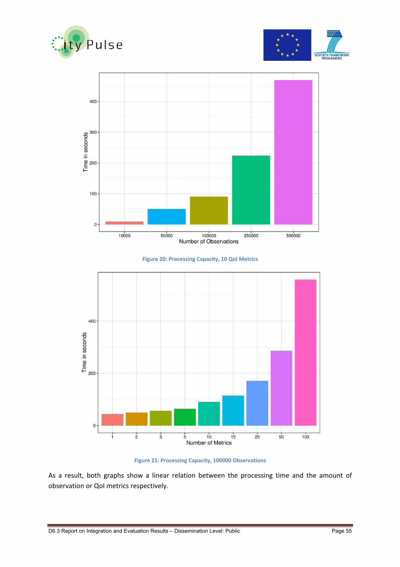
D6.3 Report on Integration and Evaluation Results – Dissemination Level: Public Page 55
Figure 20: Processing Capacity, 10 QoI Metrics
Figure 21: Processing Capacity, 100000 Observations
As a result, both graphs show a linear relation between the processing time and the amount of
observation or QoI metrics respectively.

D6.3 Report on Integration and Evaluation Results – Dissemination Level: Public Page 56
3.2.1.3.3 RAMUtilisationTo measure the RAM Utilisation of the Atomic Monitoring, the system is fed with 10000 copies of
exemplary observations. The number of metrics is increased from 0 to 1000. After the calculated
quality data is published to the other framework components, it is discarded (it is directly used to
create the annotation before being deleted), as it would be in a real deployment.
Figure 22: RAM Utilisation
Figure 22 shows the memory consumption of the Quality System in Megabytes. It can be seen that
the memory consumption stays on a constant level after about the first 1000 observations. This is a
result of not saving the complete historical behaviour of a data stream within the Atomic
Monitoring’s metrics. Their internal buffers contain only simple data types, which is limited in size
(ring‐buffer).
3.2.1.3.4 HDDUtilisationThe HDD Utilisation is negligibly small as the Atomic Monitoring consists only of some smaller
python files. The Quality System itself saves no data, does not consume any memory on a HDD/SSD.
3.2.1.3.5 Jitter/ProcessingLatencyTo measure the Jitter, observations are provided to the Quality System, and the time between
insertion and completing the processing is measured.
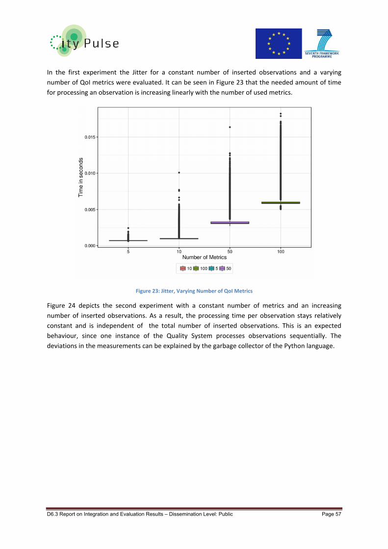
D6.3 Report on Integration and Evaluation Results – Dissemination Level: Public Page 57
In the first experiment the Jitter for a constant number of inserted observations and a varying
number of QoI metrics were evaluated. It can be seen in Figure 23 that the needed amount of time
for processing an observation is increasing linearly with the number of used metrics.
Figure 23: Jitter, Varying Number of QoI Metrics
Figure 24 depicts the second experiment with a constant number of metrics and an increasing
number of inserted observations. As a result, the processing time per observation stays relatively
constant and is independent of the total number of inserted observations. This is an expected
behaviour, since one instance of the Quality System processes observations sequentially. The
deviations in the measurements can be explained by the garbage collector of the Python language.

D6.3 Report on Integration and Evaluation Results – Dissemination Level: Public Page 58
Figure 24: Jitter, Varying Number of Observations
3.2.1.4 ConclusionThe experiments conducted with the Atomic Monitoring of the Quality System show that the RAM
Utilisation as well as the Processing Latency for inserted observation increase linearly with the
number of QoI metrics calculated in the Atomic Monitoring. The following measurements are done
with 100000 observations calculating the mean Processing Latency or RAM Utilisation respectively.
Figure 25: Time Consumption Related to Number of QoI Metrics

D6.3 Report on Integration and Evaluation Results – Dissemination Level: Public Page 59
Figure 25 shows a linear behaviour for the amount of time needed for an observation to be
processed in relation to the number of QoI metrics in the Atomic Monitoring. Figure 26 indicates a
linear RAM Utilisation with an increasing number of used QoI metrics.
Figure 26: Memory Consumption Related to Number of QoI Metrics
3.2.2 CompositeMonitoring
3.2.2.1 Testing
3.2.2.1.1 TestEnvironmentAll evaluations have been conducted using the following equipment:
Intel Core i7‐5820K, 3.6ghz, 32GB RAM
32GB RAM system memory
Historical data stored on a Solid State Disk in a PostgreSQL database
All experiments were executed by utilising a maximum of 10 Threads in parallel.
3.2.2.1.2 Testing/KPISelectionTable 7 lists a selection of the KPIs from D2.1 suitable for this innovation. The table consists of a
short description how the KPI will be measured or a justification of why the KPI cannot be measured.
Innovation Real‐time QoI Annotation
Selected KPIs How to measure?
Processing Capacity Measure the duration needed for different configurations of the component.
Processing Robustness See results in D5.2
RAM RAM utilisation while annotating observations with varying number of QoI metrics.
CPU CPU utilisation of the Composite Monitoring during runtime.
HDD Size of data sets that are used to compare. Table 8: KPI Selection for Real‐time QoI Annotation
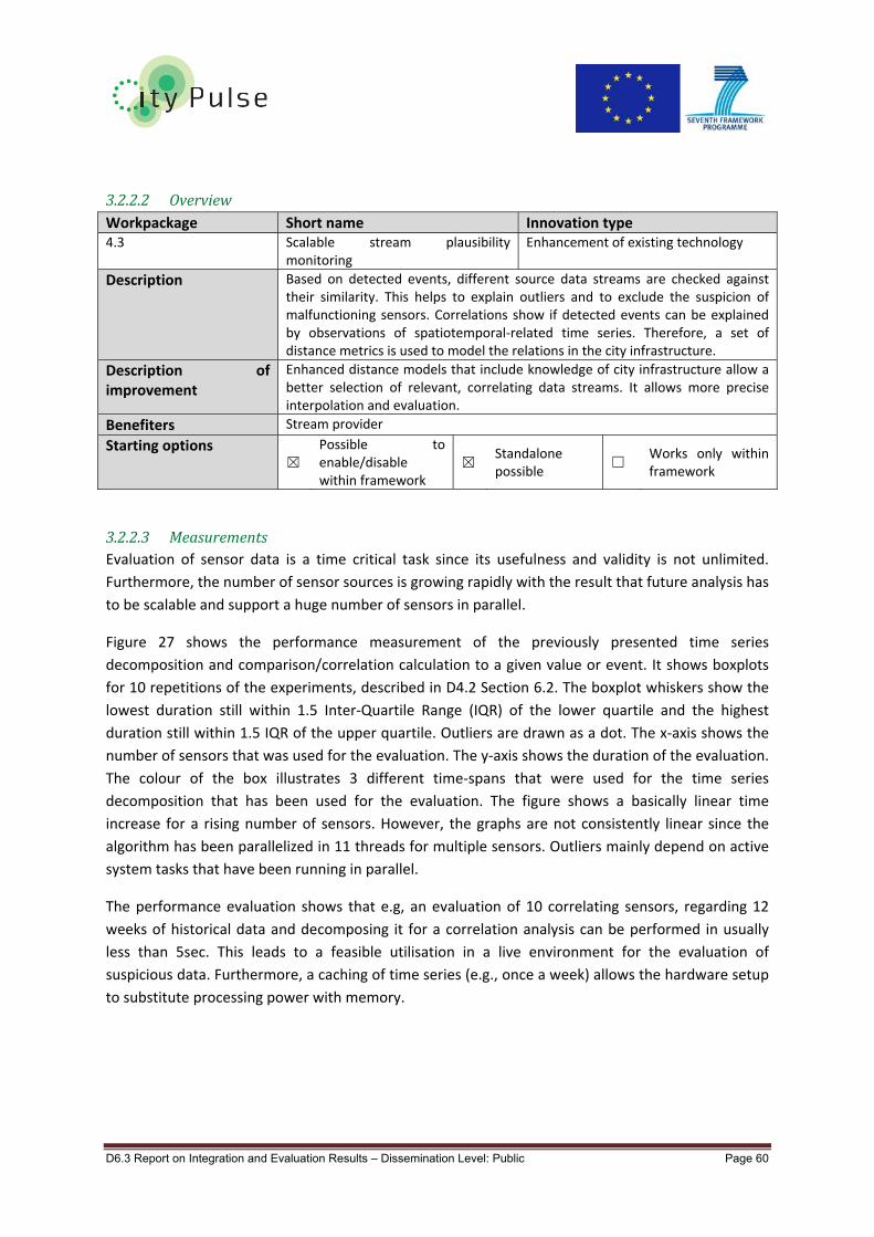
D6.3 Report on Integration and Evaluation Results – Dissemination Level: Public Page 60
3.2.2.2 OverviewWorkpackage Short name Innovation type 4.3 Scalable stream plausibility
monitoring Enhancement of existing technology
Description Based on detected events, different source data streams are checked against their similarity. This helps to explain outliers and to exclude the suspicion of malfunctioning sensors. Correlations show if detected events can be explained by observations of spatiotemporal‐related time series. Therefore, a set of distance metrics is used to model the relations in the city infrastructure.
Description of improvement
Enhanced distance models that include knowledge of city infrastructure allow a better selection of relevant, correlating data streams. It allows more precise interpolation and evaluation.
Benefiters Stream provider
Starting options ☒
Possible to enable/disable within framework
☒ Standalone possible
☐ Works only within framework
3.2.2.3 MeasurementsEvaluation of sensor data is a time critical task since its usefulness and validity is not unlimited.
Furthermore, the number of sensor sources is growing rapidly with the result that future analysis has
to be scalable and support a huge number of sensors in parallel.
Figure 27 shows the performance measurement of the previously presented time series
decomposition and comparison/correlation calculation to a given value or event. It shows boxplots
for 10 repetitions of the experiments, described in D4.2 Section 6.2. The boxplot whiskers show the
lowest duration still within 1.5 Inter‐Quartile Range (IQR) of the lower quartile and the highest
duration still within 1.5 IQR of the upper quartile. Outliers are drawn as a dot. The x‐axis shows the
number of sensors that was used for the evaluation. The y‐axis shows the duration of the evaluation.
The colour of the box illustrates 3 different time‐spans that were used for the time series
decomposition that has been used for the evaluation. The figure shows a basically linear time
increase for a rising number of sensors. However, the graphs are not consistently linear since the
algorithm has been parallelized in 11 threads for multiple sensors. Outliers mainly depend on active
system tasks that have been running in parallel.
The performance evaluation shows that e.g, an evaluation of 10 correlating sensors, regarding 12
weeks of historical data and decomposing it for a correlation analysis can be performed in usually
less than 5sec. This leads to a feasible utilisation in a live environment for the evaluation of
suspicious data. Furthermore, a caching of time series (e.g., once a week) allows the hardware setup
to substitute processing power with memory.

D6.3 Report on Integration and Evaluation Results – Dissemination Level: Public Page 61
Figure 27 Exemplarily Processing Times for Loading, Decomposing Comparing Time Series to Events
Figure 28 shows the memory consumption for the parallelised (11 threads) analysis of 1‐449 traffic
sensors with historical data of 6, 12 and 24 weeks. As a conclusion we can see that a comparison
against 449 Sensors with time series decompositions of 24 weeks of historical data can be easily
achieved with a state of the art server that is equipped with 16GB RAM.
3.2.2.4 ProcessingCapacity
Figure 28 Memory Consumption for 1‐449 Sensors and 6, 12 and 24 Weeks of Decomposed Time Series

D6.3 Report on Integration and Evaluation Results – Dissemination Level: Public Page 62
3.2.3 FaultrecoveryThe fault recovery, which is evaluated in this document, is a part of the CityPulse framework. The
Fault recovery component ensures continuous and adequate operation of the CityPulse application
by generating estimated values for the data stream when the quality drops or it has temporally
missing observations. When the quality of the data stream is low for a longer time period, an
alternative data source has to be selected. The selection can be performed automatically by the
Technical adaptation component. In other words, the technical adaptation process does not have to
be triggered if the QoI of a stream is low only for a short period of time because the Fault recovery
component provides estimated values.
3.2.3.1 OverviewWorkpackage Short name Innovation type 4.2 Ability to recover from faulty sensor
data Enhancement of existing technology
Description The Fault Recovery module is implemented with a K nearest neighbour algorithm. By continuous updates of the training data set, this module is able to estimate missing values in real‐time.
Description of Improvement
Real‐time integration of the K nearest neighbour algorithm to enable the CP framework to replace missing/wrong sensor values in real‐time.
Benefiters Application developer, citizen
Starting options ☒
Possible to enable/disable within framework
☒ Standalone possible
☐ Works only within framework
3.2.3.2 Testing
3.2.3.2.1 Testing/KPISelectionTable 7 lists a selection of the KPIs from D2.1 suitable for this innovation. The table consists of a
short description of how the KPI will be measured or a justification of why the KPI cannot be
measured.
Innovation Real‐time QoI Annotation
Selected KPIs How to measure?
Precision The prediction precision has to be assessed.
Environmental Operation Constraints
The component needs a defined input form (JSON format used within the Resource Management).
End‐to‐End Delay Measure the time between the input of a new observations and the completion of the prediction and of the training activities
Processing Latency See End‐to‐End Delay.
Processing Reliability Evaluate prediction precision compared to the missing data rate.
Processing Robustness See Processing Reliability.
RAM RAM utilization of one instance of fault recovery. Table 9: KPI Selection for Real‐time QoI Annotation

D6.3 Report on Integration and Evaluation Results – Dissemination Level: Public Page 63
3.2.3.2.2 TestEnvironmentAll KPI evaluations have been conducted using the following equipment:
Intel(R) Core(TM) i7‐2620M CPU @ 2.70GHz
16GB memory
All experiments were executed on a single core of the CPU as multi‐threading is not supported by
the fault recovery for a single Data Wrapper.
3.2.3.3 MeasurementsFor all the tests, a historical traffic data set was used. It was collected from a traffic sensor from the
city of Aarhus and contained 70,000 observations representing the average speed of the cars.
3.2.3.3.1 ProcessingReliability/ProcessingRobustnessThe Processing Reliability for fault recovery represents to the prediction error of the component,
which in our tests was measured as the mean square error. Figure 29 depicts the variation of the
prediction error versus the size of the test set.
Figure 29: Fault recovery prediction error.
Since the fault recovery component is constructing a reference dataset when the QoI of the data
stream is high, which makes it prone to missing data. Considering a dataset having 40000 (as subset
of the above‐mentioned test set), we have artificially injected missing values and tested the
performance of the fault recovery component. Figure 30 presents the prediction error variation
based on missing observation rate.

D6.3 Report on Integration and Evaluation Results – Dissemination Level: Public Page 64
Figure 30: Fault recovery prediction error variation based on missing observations rate
3.2.3.3.2 End‐to‐EndDelayFigure 31 and Figure 32 depict the processing times needed by the fault recovery component during
the training and prediction activities, respectively.
Figure 31: Fault recovery time needed for training

D6.3 Report on Integration and Evaluation Results – Dissemination Level: Public Page 65
Figure 32: Fault recovery time needed for generating predictions
3.2.3.3.3 RAMUtilisationA fault recovery instance has to be deployed within each data wrapper of the framework. One
instance contains a reference data set containing 100 lines and 5 columns, which is maintained and
used for generating predictions. As a result, the memory consumption of all fault recovery instances
is direct proportional with the reference data set size and the number of instances.
3.2.3.4 ConclusionThe experiments conducted with the Fault recovery show that the processing time used by the fault
recovery component during training and execution is linear proportional with the size of the test
data set. The prediction error for the considered data set is constant, a little bit higher than 5,
regardless of the data set size. In addition, the missing observation does not have a huge impact on
the prediction precision.

D6.3 Report on Integration and Evaluation Results – Dissemination Level: Public Page 66
3.2.4 EventdetectionThe component is able to process raw (annotated) and aggregated observation in order to detect
useful events for the user. The event detection component is generic and the user can deploy
custom developed detection patterns. This code can be used to deploy/execute custom event
detection logic. The application developer can, at any time, trigger the deployment of these
mechanisms in order to analyse the data coming from the city. In addition, the application developer
can develop custom made event detection logic by implementing a java interface.
3.2.4.1 OverviewWorkpackage Short name Innovation type 3.4 Event detection Enhancement of existing technology
Description The stream Event detection component provides the generic tools for processing the annotated as well as aggregated data streams to obtain events occurring into the city. Using this component, the application developers have only to define the event detection logic. They do not have to develop any specific codes to acquire, interpret and validate the data, as it has to be done in a traditional event driven application. This is achieved by leveraging the data wrapper and resource management mechanisms. The event detection can integrate machine learning models in order to support prescriptive analytics mechanisms.
Description of Improvement
‐integration of event detection component with data wrapper and resource management, simplifying in this way the work of the application developers ‐ prescriptive analytics functionality of the event detection (under development at this moment).
Benefiters Application developer, stream provider
Starting options ☒
Possible to enable/disable within framework
☐ Standalone possible
☒ Works only within framework
3.2.4.2 Testing
3.2.4.2.1 Testing/KPISelectionTable 7 lists a selection of the KPIs from D2.1 suitable for this innovation. The table consists of a
short description of how the KPI will be measured or a justification of why the KPI cannot be
measured.
Innovation Real‐time QoI Annotation
Selected KPIs How to measure?
Precision It is important to validate the precision of the component (number of false positives and false negatives)
Processing Latency The time needed to process a certain amount of events
RAM RAM utilization during the event detection operation. Table 10: KPI Selection for Real‐time QoI Annotation
3.2.4.2.2 TestEnvironmentAll KPI evaluations have been conducted using the following equipment:
Intel(R) Core(TM) i7‐4810MQ CPU @ 2.80GHz
16GB memory

D6.3 Report on Integration and Evaluation Results – Dissemination Level: Public Page 67
All experiments executed on a single core of the CPU as multi‐threading are not supported by the
event detection component. Within the CityPulse framework an instance of the Event Detection is
instantiated and runs on its own thread.
3.2.4.3 MeasurementsFor all the tests, a historical traffic data set was used. It was collected from a traffic sensor from the
city of Aarhus that contained 60,000 observations representing the average speed of the cars and
their density.
3.2.4.3.1 ProcessingReliability/ProcessingRobustnessFigure 33 depicts the processing times needed by the event detection component to process
different volumes of observations (from 10000 to 60000) using only one event detection node.
Figure 33: Event detection time needed for processing observations using one event detection node
Figure 34 depicts the processing time needed by the event detection component to process 40000
observations while varying the number of event detection nodes (from 1 to 1000).
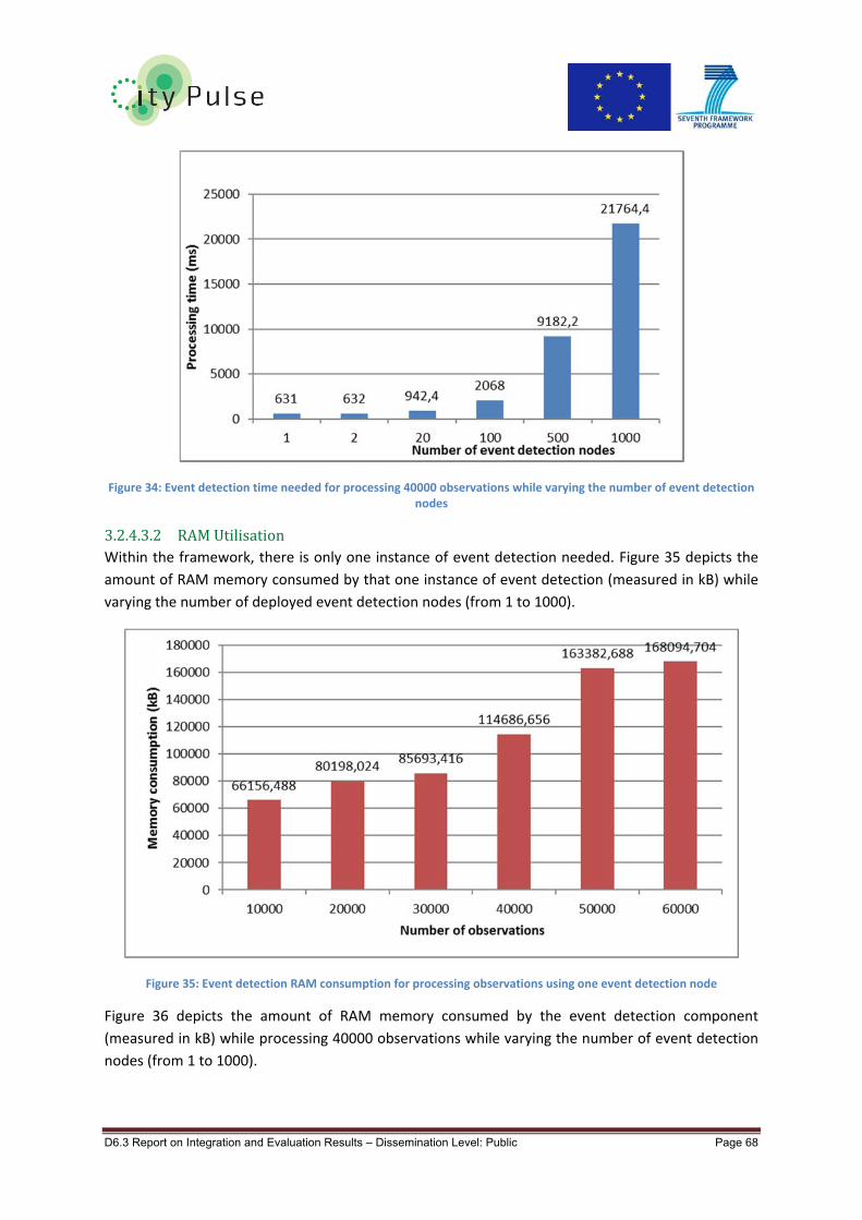
D6.3 Report on Integration and Evaluation Results – Dissemination Level: Public Page 68
Figure 34: Event detection time needed for processing 40000 observations while varying the number of event detection nodes
3.2.4.3.2 RAMUtilisationWithin the framework, there is only one instance of event detection needed. Figure 35 depicts the
amount of RAM memory consumed by that one instance of event detection (measured in kB) while
varying the number of deployed event detection nodes (from 1 to 1000).
Figure 35: Event detection RAM consumption for processing observations using one event detection node
Figure 36 depicts the amount of RAM memory consumed by the event detection component
(measured in kB) while processing 40000 observations while varying the number of event detection
nodes (from 1 to 1000).

D6.3 Report on Integration and Evaluation Results – Dissemination Level: Public Page 69
Figure 36: Event detection RAM consumption for processing 40000 observations while varying the number of event detection nodes
3.2.4.3.3 PrecisionThe precision of the component has been tested and if there are no missing observations, it is able
to correctly detect all patterns (zero false positive and false negative detected events).
3.2.4.4 ConclusionThe stress tests demonstrated that the event detection component can be used for processing the
data from a smart city environment. The component which was running on a commodity computer
was able to process large amounts of data very fast.
3.2.5 SemanticAnnotationUtilisation of semantic technologies for IoT advances interoperability among IoT resources,
information models, data providers and consumers. In an effort to reach a common consensus on a
standardisation of semantic descriptions of sensor networks, an ontology has been developed by the
W3C Semantic Sensor Network Incubator group (i.e. W3C SSN Ontology). Most of the current
ontology development methods still require tremendous effort and subjective judgments from the
ontology developers to acquire, maintain and validate the ontology.
On the one hand, the ability to design and maintain ontologies requires expertise in both the domain
of the application and the ontology language used for modelling. However, with their growing
utilisation not only the number of available ontologies has increased considerably but is also
becoming larger and more complex to manage.
On the other hand, although there has been numerous work on publishing linked‐data on the
semantic web and ontology development methodologies in order to transform the art of building
ontologies into an engineering activity; ontology and linked‐data validation process is another crucial
problem since developers need to tackle a wide range of difficulties when modelling and validating
ontologies. These difficulties, such as the appearance of anomalies in ontologies or the technical
quality of ontology against a frame reference, play a key role in the ontology engineering projects.
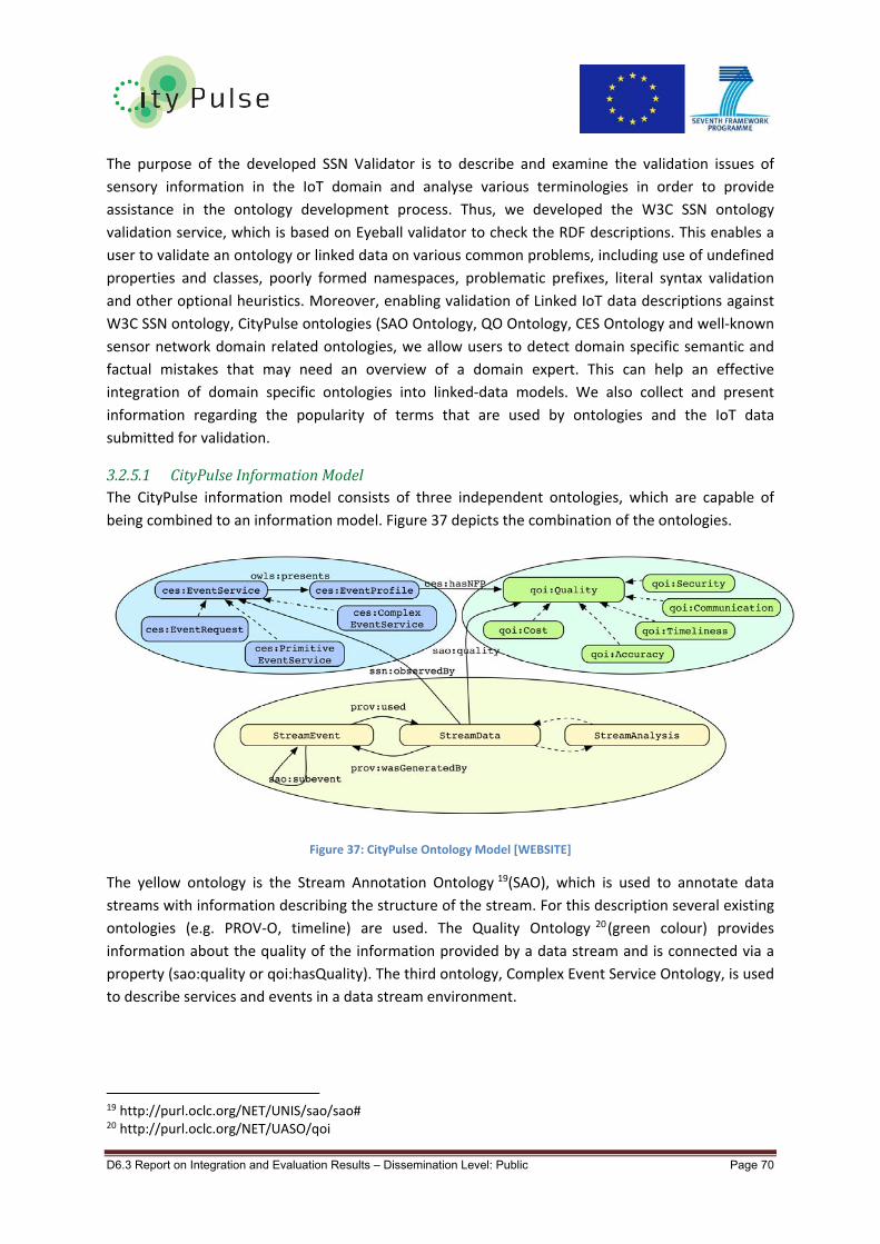
D6.3 Report on Integration and Evaluation Results – Dissemination Level: Public Page 70
The purpose of the developed SSN Validator is to describe and examine the validation issues of
sensory information in the IoT domain and analyse various terminologies in order to provide
assistance in the ontology development process. Thus, we developed the W3C SSN ontology
validation service, which is based on Eyeball validator to check the RDF descriptions. This enables a
user to validate an ontology or linked data on various common problems, including use of undefined
properties and classes, poorly formed namespaces, problematic prefixes, literal syntax validation
and other optional heuristics. Moreover, enabling validation of Linked IoT data descriptions against
W3C SSN ontology, CityPulse ontologies (SAO Ontology, QO Ontology, CES Ontology and well‐known
sensor network domain related ontologies, we allow users to detect domain specific semantic and
factual mistakes that may need an overview of a domain expert. This can help an effective
integration of domain specific ontologies into linked‐data models. We also collect and present
information regarding the popularity of terms that are used by ontologies and the IoT data
submitted for validation.
3.2.5.1 CityPulseInformationModelThe CityPulse information model consists of three independent ontologies, which are capable of
being combined to an information model. Figure 37 depicts the combination of the ontologies.
Figure 37: CityPulse Ontology Model [WEBSITE]
The yellow ontology is the Stream Annotation Ontology 19(SAO), which is used to annotate data
streams with information describing the structure of the stream. For this description several existing
ontologies (e.g. PROV‐O, timeline) are used. The Quality Ontology 20(green colour) provides
information about the quality of the information provided by a data stream and is connected via a
property (sao:quality or qoi:hasQuality). The third ontology, Complex Event Service Ontology, is used
to describe services and events in a data stream environment.
19 http://purl.oclc.org/NET/UNIS/sao/sao# 20 http://purl.oclc.org/NET/UASO/qoi

D6.3 Report on Integration and Evaluation Results – Dissemination Level: Public Page 71
3.2.5.2 Pre‐semanticvalidationwiththeSensorAnnotationLibrary:SAOPYIncreasing amount of ontologies and Linked Data resulted in an unacceptable quantity of noise
within the Web of Data which inhibits applications from effectively exploiting this rich open, well‐
defined and structured information. In [46] that there is still a vast amount of erroneous Linked
Datasets available on the Semantic Web. Although validators are useful to verify syntactical
consistency and correctness, they cannot detect domain specific semantic or factual mistakes that
may need an overview of domain specific ontologies. We address this issue by providing a sensor
annotation library, called SAOPY21 that embodies well‐known ontologies in the domain of sensor
networks. It aims to prevent common syntax errors [46] (e.g. undefined properties and classes,
poorly formed namespaces, problematic prefixes, literal syntax) in RDF documents during the
annotation process before it is published as linked data. Figure 38 illustrates how the SAOPY library
works as a pre‐ or real‐time validator during the semantic annotation process of sensory data.
Figure 38: An illustration of the pre‐validation (real‐time) validator during the semantic annotation process using the SAOPY library.
3.2.5.3 Post‐semanticvalidationwiththeSSNValidationToolFigure 39 presents the architecture of the SSN Validation Tool. The W3C SSN validation web
application integrates the ontology and data validation functionalities in web‐based client‐server
architecture. The client runs in most popular web browsers and provides an easy to use interface. It
allows the user to interact with the application and perform the following actions: i) enter an RDF
document into a text box or upload via a browse button to be validated against a reference ontology
(i.e. in this case the W3C SSN ontology, CityPulse ontologies and other well‐known ontologies such
as FOAF) ii) retrieve a list of evaluation results, iii) select and see namespaces of a term from the tag
clouds as one would do from a search engine and also visualise the most common terms and
concepts used in the ontologies.
Figure 39: The architecture of the SSN Validator web application
21 http://iot.ee.surrey.ac.uk/citypulse/ontologies/sao/saopy.html

D6.3 Report on Integration and Evaluation Results – Dissemination Level: Public Page 72
Front‐End: The validator application is developed using Java EE, HTML, JSP technologies. It takes an
RDF input or ontology to produce a set of evaluation results. The web user interface consists of a
single view where the user enters the RDF data into a text box or uploads via a browse button. In
response to user interaction, the server performs the core functionalities as shown in Figure 39.
Concerning client‐server communication, the validator follows the Representational State Transfer
(REST) style web application design. In this architecture web pages form a virtual state machine,
allowing a user to progress through the application by entering or uploading an RDF document,
which results in a transition to the next state of the application by transferring a representation of
that state to the user.
Back‐End: There are three main functionalities in the main system, namely RDF Parser, Extraction of
Terms, and Validation. Initially, the RDF document describing the ontology or RDF document is
parsed using the Jena API to obtain RDF triples as an input to the validation system. The server side
of the SSN Validation web application builds on the Eyeball validator, which is a Java library for
validating RDF documents. This is extended with modules to domain specific analysis for the W3C
SSN ontology. It scans for errors from those available in the Eyeball list regarding RDF, Turtle and N3
syntax, and some modelling suggestions are also generated.
The validation results are displayed by means of the web user interface showing a list of errors, and
explanations regarding the ontology elements affected. The application also reports the recurrence
of terms that are not present within the W3C SSN ontology. We have developed a server‐side
JavaScript code that interacts with the embedded Tag Cloud to display extracted terms that are not
present in the W3C SSN ontology. The terms requested when the user starts the validation process,
and returned using JavaScript Object Notation with evaluation results, which is presented at the
same time with extracted terms as tag cloud. The term recurrence tags are displayed using an
adapted version of the WP‐Cumulus Flash‐based Tag Cloud plug‐in. This plug‐in utilises XML data
generated on the server side from the extracted terms. The lightweight client uses a combination of
standard web technologies (HTML, CSS, JavaScript) and uses a Java library to dynamically load
content from an object‐oriented database (i.e. DB4o).
3.2.5.4 TheOntologyValidationsWe collected a set of available ontologies and semantic description models that report using and/or
extending the W3C SSN ontologies. The ontology dataset includes the Smart Product Ontology22, the
SPITFIRE project ontology23, The IoT.est project service24 model, The SemSorGrid4Env project
ontology25, The OntoSensor ontology26, The WSML Event Observation27 ontology, The WSML
Environment Observation Ontology28.
22 http://www.w3.org/2005/Incubator/ssn/wiki/SSN\_Smart\_product 23 http://spitfire-project.eu/ontology.owl 24 http://personal.ee.surrey.ac.uk/Personal/P.Barnaghi/ontology/OWL-IoT-S.owl 25 http://www.semsorgrid4env.eu/ontologies/CoastalDefences.owl 26 https://www.memphis.edu/eece/cas/onto\_sensor/OntoSensor.txt 27 https://code.google.com/p/wsmls/source/browse/trunk/global/Observations/0.2/\\Observation.n3?spec=svn70\&r=70 28 https://code.google.com/p/wsmls/source/browse/trunk/global/Event-
observation/0.2/EventObservation.n3?spec=svn207\&r=207

D6.3 Report on Integration and Evaluation Results – Dissemination Level: Public Page 73
We evaluated these ontologies using our validation tool to find out the noise, inconsistency and
syntax errors along with the similarity between the W3C SSN concepts and the terms and concepts
used in these ontologies. It can be difficult for an ontology engineer to identify some errors and
unexpected incorrect inferences in RDF. In the RDF data model, terms are typically named by Web
URIs, which may be dereferenced to access more information such as vocabulary definitions about
their meaning. However, while the principal notion behind the Semantic Web is to experience a
machine‐oriented world of Linked Data, ontology engineers should be very cautious to prevent
broken links as well as make URIs dereferencable in order to empower automatic data access for
Semantic Web applications. In accordance with the use of HTTP URIs, we found in our validations
that in some instances (i.e. WSML event and WSML environment) different URIs were utilised rather
than primary resources. As a result, it redirects the application user to their local directory instead of
original locations such as SSN Ontology. Some other errors were identified in IoT.est model and
SemSorGrid4Env, in which multiple prefixes were defined (i.e. owl and CoastalDefences,
respectively), in addition to utilisation [48] of upper case in namespaces of IoT.est model (i.e.
http://www.loa‐cnr.it/ontologies/DUL.owl#). It is interesting to see that while the latter is not
actually wrong, it is accepted as unconventional and pointless for eyeball tool.
In parallel, sometimes properties or classes are used without any formal definition. In SPITFIRE, for
instance, it has been defined that :savedEnergyOf rdfs:domain :SavedEnergy, even though
:SavedEnergy is not defined as a class. Nevertheless, although such practice is not prohibited, such
ad‐hoc undefined classes and properties make automatic integration of data less efficient and
prevent the possibility of making inferences through reasoning. An additional error that has been
found for SPITFIRE via our validation tool is a syntax error where ssn:subPropertyOf was used instead
of rdfs:subPropertyOf. Finally, we discovered in OntoSensor that there was clearly a misuse of
functional property syntax along with a data property. It needs to be updated in line with OWL‐2
guidelines using FunctionalDataProperty that describes properties for each individual allowing for at
most one distinct literal.
Table 11: Summary of ontology evaluations against the W3C SSN ontology
Table 11 summarises the results of similarity of terms and shows statistics using the W3C SSN
ontology concepts in these ontologies. We found that the most frequently used SSN terms are as
follows: Property, Device, Observation, FeatureOfInterest, and ObservationValue. Based on the
validation results, we also created a Tag Cloud that shows the most common concepts that are used
in the validated ontologies. We also checked linked ontologies and other common description
models that can be used in the form of linked‐data.

D6.3 Report on Integration and Evaluation Results – Dissemination Level: Public Page 74
Considering the most common concepts and properties that are used from the W3C SSN ontology
can help to create an optimum core ontology in which the main concepts and properties are used in
several other related ontologies. This can also give an indication of which parts of the SSN ontology
are used more than others. The latter can provide feedback to the ontology developers to help them
focus on the most commonly used features and create automated tools and software that can
enhance and increase interoperability across different applications and systems in the IoT domain.
3.2.5.5 DiscussionWe developed two different tools to tackle the semantic validation issues, namely SAOPY and SSN
Validator. While the former deals with the syntax and semantic violations in real‐time, the latter
provides an opportunity to validate data streams’ post‐annotation process. We used the SSN
Validation tool to validate a set of ontologies that are available online in which the W3C SSN
ontology was used as a base ontology. We created a Tag Cloud and presented the most common
terms and concepts that are used from the W3C SSN ontology and provided statistics regarding the
number of concepts and properties that are adapted from the SSN model in each of the ontologies.
The validation service can be used for checking and evaluating the new ontologies against base line
ontologies; e.g. the W3C SSN ontology and CityPulse ontologies. It can be also used to collect
information and statistics about the use of the W3C SSN ontology and provide feedback to the
ontology developers.
3.2.6 DataAggregationOne of the key issues in heterogeneous ecosystem of smart cities is real‐time traffic data analysis.
Enabling smart cities to efficiently manage traffic and parking data and provide alternative routes
will not only help reduce transportation cost but also pollution caused by traffic congestion.
As a use case scenario, we use public traffic5 and parking data6 that have been obtained from the
city of Aarhus in Denmark. Our experimental dataset consists of two sets of stream samples: (i)
traffic sensor observations (i.e. average speed and vehicle count) (ii) parking sensor observations
(vehicle count), which are collected during October 2014. We chose these two sets of sensory data
to compare one set with higher sampling frequency with one set at a low frequency. Each traffic
sensor has been reported to the system every 5 minutes, and each parking sensor has been reported
to the system approximately every 30 to 35 minutes. In total, there are 449 traffic and 8 parking
sensors that are turned into open data. The performance of the stream‐processing framework is
evaluated by changing the settings of SAX and SensorSAX to examine the effects (i.e. change) on the
output, namely Time, CPU%, data size, and reconstruction rate (RCR) obtained by using Euclidean
distance between the original and the reconstructed data for sensory observations, namely average
speed (AvgSpd) and vehicle count (VcCnt). In the rest of the paper, we will use the abbreviations of
RCR‐AvgSpd and RCR‐VcCnt for the reconstruction rate of average speed and vehicle count
observations, respectively.
In addition, we tested the effect of minimum window size (MWS) and sensitivity level (SL)
parameters of SensorSAX algorithm in stream processing and aggregation. The level of accuracy
estimated by these metrics is analysed utilising a one‐way Analysis of Variance (ANOVA). The
independent variables were Time (in seconds), CPU percentage, data size (in MegaByte), and
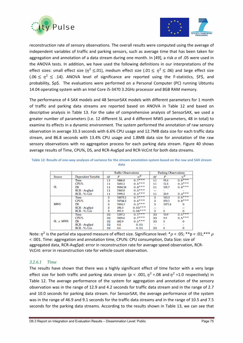
D6.3 Report on Integration and Evaluation Results – Dissemination Level: Public Page 75
reconstruction rate of sensory observations. The overall results were computed using the average of
independent variables of traffic and parking sensors, such as average time that has been taken for
aggregation and annotation of a data stream during one month. In [49], a risk of .05 were used in
the ANOVA tests. In addition, we have used the following definitions in our interpretations of the
effect sizes: small effect size ( .01), medium effect size (.01 .06) and large effect size (.06 .14). ANOVA level of significance are reported using the F‐statistics, $F$, and probability, $p$. The evaluations were performed on a Personal Computer (PC) running Ubtuntu
14.04 operating system with an Intel Core i5‐3470 3.2GHz processor and 8GB RAM memory.
The performance of 4 SAX models and 48 SensorSAX models with different parameters for 1 month
of traffic and parking data streams are reported based on ANOVA in Table 12 and based on
descriptive analysis in Table 13. For the sake of comprehensive analysis of SensorSAX, we used a
greater number of parameters (i.e. 12 different SL and 4 different MWS parameters, 48 in total) to
examine its effects in a dynamic environment. The system performed the annotation of raw sensory
observation in average 33.3 seconds with 6.6% CPU usage and 12.7MB data size for each traffic data
stream, and 86.8 seconds with 13.4% CPU usage and 1.8MB data size for annotation of the raw
sensory observations with no aggregation process for each parking data stream. Figure 40 shows
average results of Time, CPU%, DS, and RCR‐AvgSpd and RCR‐VcCnt for both data streams.
Table 12: Results of one‐way analyses of variance for the stream annotation system based on the raw and SAX stream data
Note: is the partial eta squared measure of effect size. Significance level: * < :05; **p < :01;*** < :001. Time: aggregation and annotation time, CPU%: CPU consumption, Data Size: size of aggregated data, RCR‐AvgSpd: error in reconstruction rate for average speed observation, RCR‐VcCnt: error in reconstruction rate for vehicle count observation.
3.2.6.1 TimeThe results have shown that there was a highly significant effect of time factor with a very large
effect size for both traffic and parking data stream (p < .001, =.08 and =1.0 respectively) in
Table 12. The average performance of the system for aggregation and annotation of the sensory
observation was in the range of 12.9 and 4.2 seconds for traffic data stream and in the range of 2.7
and 10.0 seconds for parking data stream. For SensorSAX, the average performance of the system
was in the range of 46.9 and 9.1 seconds for the traffic data streams and in the range of 10.5 and 7.5
seconds for the parking data streams. According to the results shown in Table 13, we can see that

D6.3 Report on Integration and Evaluation Results – Dissemination Level: Public Page 76
there was a highly significant change in terms of time cost for aggregation and annotation with SAX
on traffic and parking data streams. While there was highly significant effect on the majority of the
SensorSAX parameters for the traffic data streams, only a few cases showed a highly significant
change for the parking data streams. For the traffic data stream performance of SensorSAX, the
results indicate that highly effect was slightly decreased to significant effect with MWS=6‐‐SL= 0.6
(p<.01), and no effect found with MWS=4‐‐SL<=0.9 and MWS=6‐‐SL>0.6.
As can be seen in Figure 40 and Table 13 that show the performance of SensorSAX on parking data,
there was a decay curve in the effect of the time factor at MWS=1, where it begins with a high
significant effect for cases of SL<=0.1 (p<.001), followed by a period of moderate decrease to
significant effect between 0.2<=SL<=0.3 (p<.01), and then to a period of small significant effect
between 0.4<=SL<=0.6 (p<.05). Additionally, there as highly significant effects for MWS=2‐‐SL<=0.05,
significant effects for MWS=2‐‐SL<=0.05‐‐SL=0.1 and MWS=4‐‐SL<=0.01 (p<.01), and small significant
effects for MWS=4‐‐SL<=0.05 and MWS=6‐‐SL<=0.01 (p<.05).

D6.3 Report on Integration and Evaluation Results – Dissemination Level: Public Page 77
Table 13: Average results for the performance of SAX and SensorSAX algorithms.
Note: Data in terms of Time, CPU%, Data Size, and Reconstruction Rate of average speed and vehicle count observations for traffic and parking data streams.

D6.3 Report on Integration and Evaluation Results – Dissemination Level: Public Page 78
While the obtained dramatic decrease in the results of SAX and SensorSAX can be explained by the
fact that data aggregation process reduces the amount of time spent on the data annotation, it is
evident that the small numbers in the SensorSAX parameters of MWS and SL increase the amount of
time spent on stream processing task up to a level where it led to even a longer time than the
annotation of raw data as we can see in the case of SensorSAX with MWS=1 and 0.01<=SL<=0.3.
It is worth to point out that although the sampling frequency of the parking data stream is half an
hour in average, which is much less frequent than the traffic data streams, since there is no fixed
sampling frequency, we had to make more frequent calls to fetch the raw data for the corresponding
time period for the parking data. This programming factor did not show any effect on the other
factors (i.e. CPU%, Data Size, RCR) of the aggregation methods due to the fact that either
segmentation time was fixed or incremental.
3.2.6.2 CPUHighly significant effect was found with a very large effect size for both traffic and parking data
streams in terms of CPU consumption (p< .001, =.08 and =0.6 respectively). While there was
highly significant effect of the SAX performance on the CPU% consumption for the traffic data
stream, no significant difference was found for the parking data streams, except the small significant
effect at WS=1h. On the contrary, the results indicate that there were only a few cases with a highly
significant effect on the CPU% for traffic data streams ‐ which were MWS=1 with 0.01<=SL<=0.5,
MWS=2 with 0.05<=SL<= 0.1, MWS = 4‐‐SL=0.3, MWS=6‐‐SL=0.2 (p<.05) ‐‐‐ and highly significant
effects found on the majority of the SensorSAX cases for the parking data streams (1< MWS<2 with
0.01<=SL<=1.00, and MWS=4 with 0.01<=SL<=0.7, except MWS=6. The computational cost of
SensorSAX with small MWS and SL values seems to be high.
For the traffic data streams, a few number of cases with high CPU% usage can be interpreted as
utilisation of small numbers in MWS and SL forms a highly sensitive system, where it adds upon the
computational cost of the raw data annotation with aggregation method and consumes a larger
percentage of the CPU. This simple fact is also reflected on the Time factor. On the other hand, the
high CPU% consumption for the parking data streams can be simply explained by the fact that
parking sensors are reported to the system with a very low frequency (i.e. every half an hour) and
they have a lower variance compared to the traffic sensors. Evidently, this is also reflected in the
data size results where there is a great deal of similarity between different sensitivity levels.
Overall, there are only a few cases where the CPU% of the aggregation methods is higher than the
raw data annotation, and the majority of these cases are very close to the raw annotation. Although
it is desirable to reduce the computational cost, it is worth to note that the general aim of sensory
devices is to reduce the communication overhead. The power consumption of computation in
sensory devices is usually significantly lower than data transmission, as given [50] [51]. Thus,
utilisation of a close CPU% value to the raw data annotation can be foreseen for IoT applications.

D6.3 Report on Integration and Evaluation Results – Dissemination Level: Public Page 79
Figure 40: Comparison of data aggregation performance
Comparison between the average time in seconds (time) measured (solid line in blue), average
CPU% (dashed green line), average data size in MegaByte (dashed red line), reconstruction rate of
average speed (RCR ‐ AvgSpd) observation (dashed purple line) and average reconstruction rate of
vehicle count (RCR ‐ VcCnt) (dashed orange line) based on Euclidean distance measured for traffic
data streams. The dashed vertical lines correspond to the different window size for SensorSAX.
Figure 40a shows the average performance of each factor for the annotation of raw data, SAX with
annotation process, and SensorSAX with annotation process computed across the traffic data
streams. Parking data streams are reported in Figure 40b. Each vertical rectangle shown on the x‐
axis represents a data aggregation model with a different parameterisation. The first dashed vertical
line represents the transition from SAX to SensorSAX approach, where the rest of the dashed vertical
lines represent the change of minimum window size parameter of the SensorSAX approach.

D6.3 Report on Integration and Evaluation Results – Dissemination Level: Public Page 80
3.2.6.3 DatasizeWe found highly significant effect and a large effect size of the aggregation methods for both the
traffic and parking data streams (p<.001, =.08 and =0.9 respectively). For the traffic data
streams, highly significant effects on the data size were seen frequently for most of the SensorSAX
parameters 1<=WS<=6 and 0.01<=SL <=0.8 (p<0.001), no effects on SL=0.9, and again significant
effects with SL=1.00 (p<0.01). However, although there were highly significant effects in the data
size with SAX‐30m<=WS<=2h (p<0.001), it is important to note that SAX with WS=4h did not show
any significant effect on the data reduction for the traffic data streams, which was lower than
expected. On the contrary, for the parking data streams there was only a small effect of SAX with
WS=4h (p<0.05) and no effect for other SAX parameters. It is suggested that this could be due to the
very low data stream sampling frequency.
Overall, while the average annotated data for 1 month observations of each sensor was 12.7MB for
traffic data streams and 1.8MB for parking data streams, SAX methods managed to reduce the data
size within the range of 3.1MB and 0.4MB and in the range of 2.5MB and 0.3MB for the traffic data
streams. SensorSAX obtained results in the range of 10.8MB and 0.1MB for the traffic data streams
and in the range of 0.8MB and 0.1E‐1MB for the parking data streams. Compared to SAX algorithm,
SensorSAX possesses more parameters, which increases the number of triples in RDF documents,
and it affects the overall data size. Considering the fact that data annotated for 1 month of traffic
observations is approximately 250M triples, it is apparent that the obtained experimental results for
the aggregated data streams are important for real‐time IoT stream processing.
3.2.6.4 ReconstructionRateThe experiments showed that there were highly significant effects with a very large effect for the
error in RCR‐AvgSpd and RCR‐VcCnt observations of the traffic data streams (p<.001, =0.5 and
=0.6), and RCR‐VcCnt observation of the parking data streams (p<.001, =.04). Reconstruction rate
results of SAX and SensorSAX (p<.001) showed a highly significant effect for both the AvgSpd and
VcCnt sensor observations for the traffic data streams, except SAX with WS=4h, where there was no
effect for the VcCnt, and SensorSAX with 3<=MWS<=4 and SL=0.9 for the AvgSpd. There was
significant effect on the former and no effect on the latter.
On the contrary, there is a noticeable difference in the reconstruction rate of the VcCnt for the
parking data streams, which can be interpreted in three categories: in the first category, there were
highly significant results for the SensorSAX with 1<=WMS<=6 and 0.01<=SL<=0.2 (p<.001), then the
results followed by significant effect for 0.3<=SL<=0.4 including WMS=1 with SL=0.5 (p<.01), and
small significant effects for most of the cases of SL=0.5 (p<.05), and no significant effect was found
for 0.6<=SL<=1.00, an exception of WMS=1 with SL=0.6 (p<.05).
Although it is acceptable to see substantially different results for the cases where 0.9<=SL<=1.00 for
the SensorSAX, there were a few cases with no effect of the SL=0.9 and a small or significant effect
of the SL=1.00. However, it is clear that additional work is required before a complete understanding
can be reached for these cases.

D6.3 Report on Integration and Evaluation Results – Dissemination Level: Public Page 81
3.2.6.5 InfluenceoftheSensorSAXparametersWe have used a two‐way analysis of variance to obtain detailed performance measurement of the
SensorSAX. The results of the ANOVA test are given in Table 14. Figure 41 depicts the overall average
results for the sensitivity and minimum window size parameters.
Table 14: Results of two‐way analyses of variance for the data aggregation of traffic and parking data streams.
Note: is the partial eta squared measure of effect size. Significance level: * < :05; **p < :01;***
< :001. SL: Sensitivity Level; MWS: Minimum Window Size.
3.2.6.5.1 SensitivityWe found highly significant and large effects of the SL on all of the measurements, namely TIME,
CPU%, DS, RCR‐AvgSpd and RCR‐VcCnt for both the traffic and parking data streams (p<.001, was
in the range of 0.3 and 0.8).
For the Time factor, overall results were lower than the annotation of raw data, which was 33.3
seconds. However, the results indicate that the performance was lower with MWS=1: it started with
longer time than the annotation of raw data and continued in the same way until SL<=0.2, and
followed by a sharp decrease in the results from 31.5 down to 9.5 seconds. The results showed that
the aggregation and annotation process took less time than the annotation of raw data for the rest
of the parameter settings of the SensorSAX. For the parking data streams, there was a smoother
decrease and all of the time measurements were below time for the annotation of the raw data.
In terms of CPU% consumption, it was possible to see a similar pattern for the parking data stream
that the results were higher than the annotation of the raw data until SL<=0.2. On the contrary, we
obtained lower CPU% only after SL>=0.6, except the anomaly at SL=02. This can be explained by the
fact that the high CPU% occurred with MWS=1, which has effected the overall results.
Additionally, for the RCR, it is apparent that the reconstruction rate shows a smoothly increasing
curve after SL=0.3 for the traffic data streams, whereas there was a sharper curve for the parking
data streams, while it was apparent beforehand that there would be a smooth curve in the overall
error of RCR. On the contrary, it was expected that the intersection point between Data Size X RCR
for the SensorSAX parameters would be between 0.1 and 0.3, but it was interesting to have such an
intersection at SL=0.7 for the SensorSAX results.

D6.3 Report on Integration and Evaluation Results – Dissemination Level: Public Page 82
Figure 41: Comparisons between the overall average performance measurements of sensitivity level (SL) and minimum window size (MWS) parameters of SensorSAX
Note: Graphs show data in terms of the average time in seconds (Time) measured (solid line in blue),
average CPU% (dashed green line), average data size in MegaByte (dashed red line), reconstruction
rate of average speed (RCR ‐ AvgSpd) observation (dashed purple line) and average reconstruction
rate of vehicle count (RCR ‐ VcCnt) (dashed orange line) based on Euclidean distance measured
depicted in Figure 41a and Figure 41b for traffic data streams, respectively – and in Figure 41c and
Figure 41d for parking data streams, respectively. The annotation of raw data streams is not shown.
3.2.6.5.2 MinimumWindowSizeHighly significant effects of the MWS were found on all of the results for the traffic data streams
(p<.001) While there was very large effect size for Time, CPU% and DS factors were in the range
of 0.5 and 0.7), it was large effect size for the RCR ‐ AvgSpd ( =0.08) and medium effect size for the
RCR‐VcCnt ( =0.03). There was highly significant effect solely with very large effect size on Time

D6.3 Report on Integration and Evaluation Results – Dissemination Level: Public Page 83
and CPU% consumption for the parking data streams (p<.001, =0.6 and =0.8, respectively).
Figure 41b shows fairly consistent results with the statistical analysis results. While the significant
effect in all results of the traffic data stream can be seen in Figure 41b, it can be observed from
Figure 41d that although there was highly significant effect of Time, it has shown a small and steady
decrease in the results of parking data streams. Similar behaviour was observed in the case of DS
and RCR, with no sudden changes.
Having no significant effect on the DS and RCR can be interpreted as while MWS is a very effective
approach for a highly frequent data, it may lose its effect at lower frequencies. This is simply because
having a low sampling frequency means that data represents a longer time period, which is more
likely to have a bigger variance in the data. Therefore, the MWS effect was lost at a lower frequency.
3.2.6.5.3 InteractionbetweensensitivityandminimumwindowsizeThe interaction between SL and MWS shows highly significant effect with very large effect size on
the Time, CPU%, and DS factors (p<.001, in range of 0.5 and 0.7) and Time and CPU% for the
parking data streams (p<.001, =0.5 for both of them). On the contrary, there was no effect of this
interaction on the DS factor of the parking data streams. It is evident that the interaction did not
show any significant effect on the RCR of neither stream types.
3.2.6.6 DiscussionsIn our experiments, we used traffic and parking data streams that report data from the same town,
with different sampling frequency and data variation. We found that in most of the cases having a
change in parameterisation of SAX and SensorSAX caused a significant change not only in the results
of data size and reconstruction rate, but also CPU% and processing time. When we take into account
all the intersection points for data aggregation processes given in Figure 40 the highest performance
was obtained for SAX with WS=1h and SensorSAX with SL=0.7 and MWS=2. While in this particular
case, SAX performed better than SensorSAX in terms of processing time, it was evident that
SensorSAX managed to reduce the size of data to the same level by decreasing the error in
reconstruction rate by a factor of 0.2 in Euclidean distance. Although this result seems to be a small
difference, it should be taken into account that SensorSAX annotation involves an additional triple
for its parameters, which can lead to a larger data reduction size for a month of data. With regard to
the Time factor, SensorSAX was yielded lower performance with most of the SL and MWS
parameters.
We found that the intersection points given in Figure 40 depict the best performance in terms of all
factors. However, when we further examined the results for each sensor individually, it is possible to
see that there is a large variation in the results of SensorSAX. Figure 42b depicts the average and
standard deviation of the sensory observations that we used in the experiments, and Figure 42a
shows the comparison between all SAX models and one of the best SensorSAX models in terms of
reconstruction rate (i.e. RCR‐AvgSpd: 0.7 and RCR‐VcCnt: 0.4 ), which could not perform as
well in terms of data reduction (i.e. data size: 10MB).

D6.3 Report on Integration and Evaluation Results – Dissemination Level: Public Page 84
Figure 42: Figure 42a illustrates a scattered representation of the results of SAX
Note: Graph shows data with WS=30m, 1h, 2h, 4h and SensorSAX with MWS=1 and SL=0.10 in terms
of data size and reconstruction rate of average speed for 449 traffic sensors. The vertical dashed line
represents the high performance variance of SensorSAX for different sensors in terms of data size.
Figure 42b depicts the graphical representation of the average (i.e. x‐axis) and standard deviation
(i.e. y‐axis) of the raw average speed traffic observations for 449 sensors.
It can be seen from this particular comparison that the results obtained by SAX models for traffic
sensors are very sparse for the reconstruction rate. This can be explained by the fact that utilisation
of fixed window size for data stream which is high in variance can dramatically reduce the data
compression quality. In the meantime, it carried out a constant behaviour for data reduction
regardless of geographical location and environmental changes of the sensors. On the other hand, it
can be seen that SensorSAX obtained very sparse results for data reduction. Despite having a better
performance with SAX for the majority of sensors, the results indicate that SensorSAX has clearly
outperformed most of the SAX models in terms of both data reduction and reconstruction rate for
some of the sensors in this particular case.
When we further investigated this issue, we found out that this was because the sensors closer to
the city centre have a larger data variation compared to the ones in the outskirts of the city. Since
SensorSAX is an adaptive segmentation approach and triggered based on events, it performs
excellent with small parameterisation in terms of reconstruction rate in high data variations, but it
cannot perform as well in high data variations in terms of data reduction, which occurred in city
centre in the experiment. Figure 43 depicts the sensors that are located in the city of Aarhus, and
one of the sensors that has been installed on the outskirts of town, which obtained excellent results
both in terms of reconstruction rate and data reduction with small parameters of SensorSAX model,
SensorSAX MWS=1 and SL=0.10. It was possible to see similar cases for approximately 30 different
sensors where there was excellent performance of SensorSAX both in reconstruction rate and data
reduction. Thus, the results indicate that the system needs to use optimum parameterisation for not
only different type of data streams, but also for the sensors of the same type of data stream that can
have different dynamicity and environmental change even though they are not very far from each
other.

D6.3 Report on Integration and Evaluation Results – Dissemination Level: Public Page 85
Figure 43: A visual representation of geographical coordinates on Google Map for road traffic sensors provided by city of Aarhus, Denmark.
Note: The sensor shown in the small circle represents location of the one of the high performance
obtained for SensorSAX with MWS=1 and SL=0.10: Time: 12.9 seconds, CPU 28%, 1.28MB for data
size, and 0.021 for RCR‐AvgSpd and 2.95E‐16 RCR ‐ VcCnt. The large circle depicts some of the
sensors closer to the city centre and higher in road traffic.
Sensors can observe more than one phenomenon in parallel, such as humidity, temperature, and in
our case average speed and vehicle count in the city road traffic. Another important factor in
adaptive segmentation of data aggregation occurred in the parallel search of optimum window sizes
for multiple observation type of the sensors. We found many cases where variances in average
speed were reached to the limit and vehicle count was still lower than the sensitivity level. Due to
the fact that we have designed our system to report the phenomena whenever either observation
reaches the sensitivity level, this was another factor that should be taken into account in such
dynamic environments as another trade‐off in the performance of the adaptive segmentation data
aggregation methods.
The results clearly demonstrate the advantage as well as disadvantage of transforming a time‐series
analysis approach from time dependent to data centric approach. There seems to be a clear trade‐
off between the two approaches.
SAX is not an adaptive segmentation approach and has to inform the system in a fixed time
frequency for an actuation even in a sudden environmental change. Furthermore, SAX needs a pre‐
processing to obtain the optimum window size, while SensorSAX dynamically adapts its window size
without the need of a training phase. On the contrary, SensorSAX enables to inform the system
when there is a change in the sensory observations. However, although SensorSAX has got many
advantages by having additional parameters to function as an adaptive segmentation method, our
experiments suggest that the system needs to use different parameters depending on the type,
frequency and distribution of data stream. There were some cases, where SensorSAX with small
numbers of SL and MWS has clearly outperformed SAX approach with compelling results in terms of

D6.3 Report on Integration and Evaluation Results – Dissemination Level: Public Page 86
reconstruction rate, but this at the same time also caused by an increase in Data Size, CPU% and
Time in stream processing.
Considering the fact that 1 month of annotated traffic data can produce approximately 250M triples,
the obtained experimental results for the aggregated data streams are suitable for real‐time IoT
systems. While the results are reported in average result of each individual sensor, it can also be
noted that the total data size for 449 annotated traffic data streams was 5.7 GB (i.e. 449 X 12.7 MB),
and it has been reduced to various data sizes that were in the range of 75.59% to 96.8% for SAX and
14.9% to 99.2% for SensorSAX with different data compression qualities and computational cost.
These numbers indicate the importance of having a better data aggregation approach with minimum
information loss, which can eventually lead to improve the performance of the applications that rely
on the abstraction and correlation techniques.
Overall, in highly dynamic environments where the system receives data streams from multiple
heterogeneous sensors, there is no ultimate parameter that can lead to perfect results for all data
streams. The parameter selection is highly dependent on the type, sampling frequency and
distribution of data stream. It is desirable to find the optimal data aggregation parameters for each
data stream, which can be obtained by training the system based on the nature of phenomena being
observed by the sensors. In addition, it is worth to point out that focusing solely on the data
reduction is not adequate for IoT stream processing. In addition to the data size and reconstruction
rate, it is evident that Time, CPU% consumption are highly significant factors in the data aggregation
process of IoT stream processing. To have a fair comparison for both approaches on the traffic and
parking data streams, we had to use the sax word size of “1” due to very low data frequency.
Nevertheless, we believe that the difference will be clearer with higher frequency of data streams,
where we can increase the word length.
3.2.7 ContextualFilteringThe contextual filtering, which is evaluated in this document, is a part of the CityPulse framework. Its
main role is to continuously identify and filter events that might affect the optimal result of the
decision making task (performed by the Decision support component), and react to such changes in
the real world by requesting the Decision support for the computation of a new solution when
needed. This not only ensures that the selected solution provided to the user remains the best
option when situations change. It also empowers the CityPulse framework to automatically provide
alternative decisions whenever the selected best decision is no longer the best for a particular
situation. The adaptive capability of identifying and reacting to unexpected events in a user‐centric
way relies on two aspects: i) a characterisation of the user implicit and explicit context provided by
the user application (including user requirements, preferences, events of interests and activities),
and ii) a stream of events provided by the Event detection component.
To measure the KPIs, an instance of the Contextual Filtering has been executed over the scenario of the travel planner with a rule set is in CityPulse deliverable D5.2. We generate traffic events based on 10 types of events such as: roadwork, obstructions, incident, sporting events, disasters, weather, traffic conditions, device status, visibility, air quality, incident response status. Each type of event has more than 2 values, e.g. traffic condition has values: good, slow, and congested. In addition to that, we use the user’s activity ontology in CityPulse deliverable D5.2 for describing the effect of events

D6.3 Report on Integration and Evaluation Results – Dissemination Level: Public Page 87
on certain activities.
3.2.7.1 OverviewWorkpackage Short name Innovation type 5.2 Contextual Filtering Enhancement of existing technology
Description Continuously identify and filter detected events that might affect users based on their context
Description of Improvement
Enhance user context ontology, provide criticality of a detected events.
Benefiters Citizen
Starting options ☒
Possible to enable/disable within framework
☐ Standalone possible
☐ Works only within framework
3.2.7.2 Testing
3.2.7.2.1 Testing/KPISelectionTable 7 lists a selection of the KPIs from D2.1 suitable for this innovation. The table consists of a
short description how the KPI will be measured or a justification why the KPI cannot be measured.
Innovation Contextual Filtering
Selected KPIs How to measure?
Environmental Operation Constraints
The component needs a defined input form (JSON format used within the Contextual Event Request).
Processing Latency The time required to reasoning over an input window
RAM RAM utilisation while annotating observations with varying number of QoI metrics.
HDD HDD utilisation
Table 15: KPI Selection
3.2.7.2.2 TestEnvironmentAll KPI evaluations have been conducted using the following equipment:
Debian GNU/Linux 6.0.10, containing 8‐cores of 2.13 GHz processor and 64 GB RAM
ASP reasoner Clingo 4.3.0 and Java 1.7
We evaluated the same ASP program with varying input size S (from 100 to 50000 events) and measured the reasoning time of the system. We trigger the reasoner 20 times for each S and then we computed the interquartile mean (IQM) to smooth results.
3.2.7.3 Measurements
3.2.7.3.1 ProcessingLatencyThe following graph illustrates the reasoning latency of the Contextual Filtering component. The
Contextual Filtering has order of n2 time complexity, where n is the size of the input window. It is
worth to note that this reasoning latency is computed as the sum of the time required for
transferring data format (between RDF and ASP syntax) and the time required for reasoning by the
Clingo solver.

D6.3 Report on Integration and Evaluation Results – Dissemination Level: Public Page 88
Figure 44: Reasoning latency
3.2.7.3.2 RAMUtilisationFigure 45 shows the memory consumption of the Contextual Filtering in Megabytes. It can be seen
that the memory consumption is less than 100 MB up to 50000 events. This is a result of not saving
the events after processing. Its internal buffers contain only simple data types, which are limited in
size.
Figure 45: Memory consumption
0
1000
2000
3000
4000
5000
6000
7000
0 5000 10000 15000 20000 25000 30000 35000 40000 45000 50000
Offlin
e Processing Time (ms)
Number of Events
82
84
86
88
90
92
94
96
5000 10000 15000 20000 25000 30000 35000 40000 45000 50000
Memory
consumed (M
B)
Number of events

D6.3 Report on Integration and Evaluation Results – Dissemination Level: Public Page 89
3.2.7.3.3 HDDUtilisationThe HDD Utilisation is negligibly small as the Contextual Filtering consists only of a small clingo file
for the set of logic rules. The Contextual Filtering itself saves no data, does not consume any
memory on a HDD/SSD.
3.2.7.4 ConclusionThe experiments conducted with the Contextual Filtering show that the RAM Utilisation is linearly
increasing while the reasoning latency has a trend of n2.
3.2.8 RewardandPunishmentalgorithmfornormalisedQoImetricsThe Reward and Punishment algorithm is implemented into the Atomic Monitoring component to
produce a rating, which indicates the current performance of a sensor. Each QoI metric for each
sensor maintains an individual instance of the algorithm. It was designed to provide a normalised
value, which allows the user to a) easily compare different sensor nodes; even from different
providers and b) to compute an overall quality based on a subset of individual QoI metrics.
The input for the algorithm is a Boolean value. The output is increased if the input was positive and
vice versa, within the value range between 0 and 1. In case of the Atomic Monitoring a positive input
is given, in case the most recent sensor reading satisfies the corresponding QoI metric constraints,
e.g. the reading is complete. The algorithm uses a window W to include past behaviour, avoiding
higher fluctuations in the output.
3.2.8.1 RAMUtilisationAs mentioned before, the Reward and Punishment algorithm uses the window W to include the
sensors past behaviour in its calculations. Since the window is implemented as ring‐buffer, the size
of the window |W| determines the RAM utilisation. Because each element in the ring‐buffer is a
Boolean value, the total memory consumption is:
Σ 1 bit * |WQ| * q * d, where
|WQ| is the window size for QoI metric Q, q is the number of QoI metrics in the Atomic Monitoring
and d is the number of Data Wrappers deployed in the Resource Management.
The following plot shows, that the memory consumption scales linearly with an increasing number of
Data Wrappers and QoI metrics. Here, with 1 million instances, having a window size of 10, less than
1 GB of memory is used. In turn, that means having four Atomic Monitoring QoI metrics, 250000
data streams can be handled per gigabyte of RAM.

D6.3 Report on Integration and Evaluation Results – Dissemination Level: Public Page 90
Figure 46: For Atomic Monitoring memory consumption scales linearly with increasing number of Data Wrappers and QoI metrics
3.2.8.2 ProcessingCapacityThrough experimental evaluation on a Apple MacBook Pro 2015 (2.8 GHz Intel Core i7, 16 GB RAM)
the authors identified that the processing capacity of the algorithm is about 325 runs per
microsecond in average for a single instance.

D6.3 Report on Integration and Evaluation Results – Dissemination Level: Public Page 91
Figure 47: Processing Capacity for Atomic Monitoring
3.2.9 DecisionSupportHere, we present the experimental evaluation of the performance of the Decision Support component in the CityPulse framework. This component utilizes contextual information available as background knowledge, user patterns and preferences from the application as well as real‐time events to provide optimal configurations of smart city applications and enable reactive smart city applications to be deployed. It is implemented based on an ASP solver. In order to provide the answers to the reasoning request, the Decision Support component collects data/knowledge from other components in the CityPulse framework such as GDI, Data Federation, and Knowledge Base. Then, it transfers these data/knowledge into facts in ASP syntax. Finally, it triggers the ASP solver for reasoning over these facts together with a set of rules given in advance in CityPulse deliverable D5.2.
We use the Travel Planner scenario as the experiment setting to measure the KPIs of the Decision
Support component. The logical rules for this scenario are documented in CityPulse deliverable D5.2.
We evaluate the Decision Support with variants concurrent numbers of reasoning requests. We
observed the reasoning time, which measured as the difference between the time when a reasoning
request is received and the time when the Decision Support component provides the answers
(optimal routes). Note that this reasoning time excludes the time that the Decision Support is
waiting for the data/knowledge from the GDI, Data Federation, and Knowledge Base.

D6.3 Report on Integration and Evaluation Results – Dissemination Level: Public Page 92
3.2.9.1 OverviewWorkpackage Short name Innovation type 5.2 Decision Support Enhancement of existing technology
Description The Decision Support component has used a declarative non‐monotonic logic reasoning approach based on Answer Set programming to utilise contextual information available as background knowledge, user constraints and preferences from the application as well as real‐time events to provide optimal solutions of smart city applications.
Description of Improvement
Automatic mapping of user's requirements to logic rules and provides optimal solutions which take into account events in the city.
Benefiters Application developer, Citizen
Starting options ☒
Possible to enable/disable within framework
☐ Standalone possible
☐ Works only within framework
3.2.9.2 Testing
3.2.9.2.1 TestingKPISelectionTable 7 lists a selection of the KPIs from D2.1 suitable for this innovation. The table consists of a
short description of how the KPI will be measured or a justification of why the KPI cannot be
measured.
Innovation Real‐time QoI Annotation
Selected KPIs How to measure?
Environmental Operation Constraints
The component needs a defined input form (JSON format).
Processing Latency The time required for the Decision Support provides answers. It excludes the time that this component waiting to collect data from GDI, Data Federation, and Knowledge Base.
RAM RAM utilisation while reasoning on variants number of reasoning requests
CPU CPU utilisation
Table 16: KPI Selection
3.2.9.2.2 TestingEnvironmentAll KPI evaluations have been conducted using the following equipment:
Ubuntu 12.10, containing 24‐cores of 2.40clear GHz processor and 64 GB RAM
ASP reasoner Clingo 4.5.4, Java 1.7, and Python 2.7.3
We evaluated the Decision Support component by varying the number of reasoning requests from 1 to 200. We use Jmeter29 to send concurrent reasoning requests.
29 We use Jmeter tool for the generation of concurrent reasoning requests with a ramp‐up time of 0.5 second.

D6.3 Report on Integration and Evaluation Results – Dissemination Level: Public Page 93
3.2.9.3 Measurements
3.2.9.3.1 ProcessingLatencyFigure 48 illustrates the reasoning latency required by the Decision Support component to handle all
concurrent reasoning requests. It is evident from the results that up to 200 concurrent reasoning
requests are all handled in less than a second.
Figure 48. Reasoning latency for handling all concurrent reasoning requests
Figure 49 shows that the average delay for each reasoning request is less than a second for all
variations in number of requests, and this time decreases as the number of requests increases. This
outcome is due to the cache optimisation mechanism of the OS on the server, which is triggered
when the number of concurrent requests is higher than the number of concurrent threads handled
by the server.
0
100
200
300
400
500
600
700
800
900
1000
1 10 50 100 200
Time (ms)
Number of reasoning requests

D6.3 Report on Integration and Evaluation Results – Dissemination Level: Public Page 94
Figure 49. Average time delay for handling all concurrent reasoning requests
3.2.9.3.2 RAMUtilisationFigure 45 shows the memory consumption of the Decision Support in Megabytes. It can be seen that
the memory consumption is less than 600 MB up to 200 concurrent reasoning requests. This is a
result of not saving the routes after processing. Its internal buffers contain only simple data types,
which are limited in size.
0
100
200
300
400
500
600
700
800
900
1 10 50 100 200
Time (ms)
Number of reasoning requests

D6.3 Report on Integration and Evaluation Results – Dissemination Level: Public Page 95
Figure 50. Memory consumption
3.2.9.3.3 HDDUtilisationThe HDD Utilisation is negligibly small as the Decision Support consists only of a small clingo file and
python file. The Decision Support itself saves no data and does not consume any memory on a
HDD/SSD.
3.2.9.4 ConclusionThe experiments conducted with the Decision Support show that the RAM Utilisation is linearly
increasing while the reasoning latency for handling concurrent reasoning requests tends to decrease
when the number of requests is higher than 50.
3.2.10 TestFrameworkCityPulse has developed a method to test the robustness of an application that uses the CityPulse
framework. The method consists of two parts: 1) the Historical Data of a data stream will be
degenerated by user defined error models in various iterations and 2) the Resource Management’s
replay mode is used to replay the degenerated Historical Data. During replay, the application uses
the faulty sensor observations or events generated by the Event Detection respectively.
3.2.10.1 Testing
3.2.10.1.1 TestEnvironmentAll evaluations have been conducted using the following equipment:
2.8 GHz Intel Core i7
16GB RAM system memory
Historical Data stored on a Solid State Disk
0
100
200
300
400
500
600
1 10 50 100 200
Memory (MB)
Number of reasoning requests

D6.3 Report on Integration and Evaluation Results – Dissemination Level: Public Page 96
3.2.10.1.2 Testing/KPISelectionTable 7 lists a selection of the KPIs from D2.1 suitable for this innovation. The table consists of a
short description how the KPI will be measured or a justification why the KPI cannot be measured.
Innovation Real‐time QoI Annotation
Selected KPIs How to measure?
Processing Latency 1. Measurement of time to degenerate one iteration of Historical Data and 2. Measurement of time to run the Resource Management in replay mode with the degenerated data.
RAM RAM utilisation while annotating observations with varying number of QoI metrics.
CPU CPU utilisation of the Composite Monitoring during runtime.
HDD Size of data sets that are used to compare.
Table 17: KPI Selection for Real‐time QoI Annotation
3.2.10.2 OverviewWorkpackage Short name Innovation type
4.3 Test framework Enhancement of existing technology
Description The test framework enables testing of applications regarding the minimal KPIs of data sources. An emulation allows the replay of reference datasets and an alteration of the information quality to investigate the limits of the application.
Description of Improvement
Reference data sets allow a realistic determination of the application limits.
Benefiters
Starting options ☐
Possible to enable/disable within framework
☒ Standalone possible
☐ Works only within framework
Description of starting options
Definition of endpoints from other components/innovations, which should be tested.
3.2.10.3 MeasurementsThe original Historical Data was imported from CSV‐files (comma separated values). The
measurements were performed using the Aarhus traffic data recorded for the development for the
Aarhus Traffic Data Wrapper and can be found in the Resource Managements GitHub repository.
The traffic data is provided by the ODAA (Open Data Aarhus) platform and contains 449 traffic
sensors. ODAA provides new observations for the traffic stream every five minutes. For the
measurements 24 hours of historicalal datasets are used.
For the degeneration of the Historical Data three errors have been modelled, namely “delay”,
“outlier” and “stuck‐at”. The Historical Data is degenerated in 100 iterations. In each iteration the
errors have a different probably to become active. The following plot shows the activation
probabilities for all iterations.

D6.3 Report on Integration and Evaluation Results – Dissemination Level: Public Page 97
Figure 51: Activation probabilities for all iterations
The stuck‐at error emulates a sensor that is stuck at a specific value. At the time of its activation a,
the error model replaces n following observations of this sensor with the value at time a. Therefore,
n is the duration of the error. The delay error emulates a sensor delivering an observation t seconds
late. t was set to 10 seconds in order to trigger a reduction of the Frequency‐QoI metric. And finally
the outlier error manipulates, when active, the observation value v by increasing it by multiplying by
seven (v * 7).
3.2.10.3.1 ProccesingLatencyThe degeneration of the Historical Data utilises the scientific data analysis framework Panda30 for the
programming language Python. The error models are designed for a sensor frequency of one second.
Therefore, in a first step the original historical data is resampled accordingly. Afterwards the
algorithm iterates over each data item and performs the following: 1) Activates an error according to
the corresponding activation probably and 2) Applies the error to the data item. This is done for the
desired number of iterations – in this case 100. Each iteration is saved into an individual CSV‐file,
which can be used as a replacement of the original historical data. The following plot shows the
Processing Latency for the first 100 traffic sensors. The average Processing Latency is 119.6 seconds.
The slight increase at the later iterations is due to the fact that those sensors provided more (about
10%) observations that need to be imported. (Those sensors worked more reliably).
30 http://pandas.pydata.org

D6.3 Report on Integration and Evaluation Results – Dissemination Level: Public Page 98
Figure 52: Processing Latency for the first 100 traffic sensors
To use the previously create degenerated historical data, the original historical data is replaced and
the Resource Managements is started in replay mode. The time it takes for the Resource
Management to run one replay depends on several factors. First, the time span that is being
replayed (here one day). Second, the deployed Data Wrappers and their update interval. Beside the
Aarhus Traffic Data Wrapper with an update interval of five minutes, the Aarhus‐Parking‐Garages
Data Wrapper was also deployed during the experiment. This Data Wrapper provides information
about the occupation level of 13 parking garages in Aarhus and has an update interval of one
minute. Lastly, the value for the Resource Management’s “speed” command line argument (see
table at https://github.com/CityPulse/Resource‐Manager) influences the replay duration. During the
measurements a value of 1000 (fastest; no delay) was used as speed. On average the Resource
Management needed 16.3 minutes to replay one day. The fastest iteration was done in 11 minutes
and 38 seconds, the slowest iteration needed 21 minutes and 51 seconds. Since the CityPulse
framework was deployed within a VirtualBox virtual machine, a better performance on native
hardware should be possible.
3.2.10.3.2 HDDUtilisationThe amount of storage required for the original historical data of all 449 traffic sensors depends on
how long the sensor observations have been recorded. Each entry in the CSV‐file consists of a
timestamp requiring 19 bytes, 3 integer numbers with up to 3 digits (3 x 3 bytes), and 3 separator
characters (‘,’) requiring also 3 bytes. In total this makes 19 bytes + 3 x 3 bytes + 3 bytes = 31 bytes
for each entry. With an update interval of 5 minutes this makes 12 x 24 x 31 bytes = 8928 bytes each
day.

D6.3 Report on Integration and Evaluation Results – Dissemination Level: Public Page 99
As the degenerated historical data is stored in the same format, it requires the same amount of disk
space. Thus, generating degenerated historical data for all 449 sensors in 100 iterations for one day
needs about 410 MB disk space.
3.2.10.3.3 CPUUtilisationThe Resource Management used during the replay run 100% of the CPU. This is due to the fact, that
the command line argument “speed” was set to 1000. This means that no delay between two replay‐
seconds is introduced. Choosing a lower speed value changes this behaviour and therefore reduces
the CPU load.
3.2.10.4 ConclusionThe Test Framework is intended to be used during the development of new CityPulse enabled
applications on a dedicated system. There, it is not able to interfere with the production system. For
this reason, runtime performance was not in focus during the development of the Test Framework.
3.2.11 DataFederationData Federation is a key function in the Smart City Framework, as it enables real‐time, collaborated,
semantic data stream processing. The data streams handled by the Data Federation component
consist of primitive data streams, e.g., sensor data streams, as well as data processing result
streams, e.g., a series of abnormal traffic readings derived from a traffic data stream. The Data
Federation components models those data and result streams as primitive and complex event
services, respectively, using the Complex Event Service Ontology31. This way, semantic discovery and
composition of data streams are realized, which allows different data stream and data stream
processing engines to collaborate with each other, even if they are implemented by different
techniques.
The Data Federation component has two key actions: 1) when a request is received, it uses the
composition algorithms provided to find optimal service compositions (data stream federations); 2)
then, the composition plans are transformed into RDF Stream Processing (RSP) queries and deployed
on RSP engines. Hence, the evaluation of the Data Federation component has two parts: the
evaluation for the design time (composition) and at run‐time (RSP query execution).
3.2.11.1 OverviewWorkpackage Short name Innovation type 3.2 Data Federation Creation of new technology
Description Federation and optimisation of heterogeneous data streams, applying RDF Stream Processing technique over those federated streams to obtain real‐time semantic stream analysing capability
Description of Improvement
Global optimisation of stream federation based on both functional and non‐functional aspects.
Benefiters Application developer, End user
Starting options ☐
Possible to enable/disable within framework
☒ Standalone possible
☐ Works only within framework
31 Complex Event Service Ontology: http://citypulse.insight‐centre.org/ontology/ces/

D6.3 Report on Integration and Evaluation Results – Dissemination Level: Public Page 100
3.2.11.2 Testing
3.2.11.2.1 Testing/KPISelectionTable 7 lists a selection of the KPIs from D2.1 suitable for this innovation. The table consists of a
short description how the KPI will be measured or a justification why the KPI cannot be measured.
Innovation Real‐time QoI Annotation
Selected KPIs How to measure?
Accuracy Measure the deviation of the actual QoS of the composition plan from the theoretical QoS (for design‐time).
Autonomy See Technical Adaptation.
Environmental Operation Constraints
The component needs a defined input form (JSON format).
End‐to‐End Delay Measure the time between a observation is produced and the corresponding RSP result is captured (for run‐time).
Processing Latency Measure the time taken to create composition plans (for design‐time).
Processing Capacity Measure the maximum number of RSP queries accepted at the same time (for run‐time).
Processing Robustness Measure the completeness of RSP query results (for run‐time).
RAM Measure the RAM utilisation while executing RSP queries (for run‐time).
Table 18: KPI Selection
3.2.11.2.2 TestEnvironmentThe evaluation of the data stream federation/composition algorithms (design‐time KPIs) are tested
using:
Intel 2.53 GHz duo core CPU and
GB 1067 MHz memory.
The evaluation of the RSP query processing engines (run‐time KPIs) are tested using:
8‐cores of 2.13 GHz intel processor and
64 GB RAM.
3.2.11.3 Measurements
3.2.11.3.1 ProcessingLatency(fordesign‐time)The Data Federation component uses a novel Genetic Algorithm (GA) designed for composing data
streams (Primitive Event Services) and data stream processing results (Complex Event Services). In
this evaluation we create 9 different service repositories (R1 to R9) with 1800 to 9000 different
event services (sensor data streams) and test the composition algorithms over them, with different
queries. The scalability, i.e., efficiency of the GA, is first compared to the Brute Force (BF)
enumeration. The results in Figure 53 indicate that the composition time of a Brute‐Force (BF)
enumeration grows exponentially with regard to the complexity of the query (number of sensors
involved) and to the number of sensors in the repository. When we apply the GA over Qb’ on R2, we
save approximately 80% of the execution time. However, for Qa and Qa’, the solution space is too
small for the GA evolution.

D6.3 Report on Integration and Evaluation Results – Dissemination Level: Public Page 101
Figure 53: Brute Force vs. Genetic Algorithm on R1 and R2
It is evident that a BF approach for QoS optimization is not scalable because of the NP‐hard nature of
the problem. The scalability of the GA is analysed using different repository sizes, queries with
different sizes (the size of a query is the sum of the number of event operators and event service
nodes), as well as different number of CESs in the Event Reusability Forest (ERF), which is the
indexing structure over the repository.
Figure 54: Genetic algorithm scalability over event service repository
The results in Figure Figure 54 show that the composition time of Qa grows linearly for GA when the
size of the repository increases. To test the GA performance with different event pattern sizes with
different operators, the EST of Qb is used as a base and replaces its leaf nodes with randomly
created sub‐trees (invalid ESTs excluded). Then the GA convergence time of these queries over R5 is
tested. The results from this experiment are detailed in Figure 55, and they indicate that the GA
execution time increases linearly with regard to the query pattern size.
1702
12305
2305
89 211
25 48
1
10
100
1000
10000
100000
R1 ‐ BF R2 ‐BF R2 ‐ GA
ms
Repositories
Qa
Qa'
Qb'
0
500
1000
1500
2000
2500
3600 4500 5400 6300 7200 8100 9000
me (ms)
repo size
min avg max

D6.3 Report on Integration and Evaluation Results – Dissemination Level: Public Page 102
Figure 55: Genetic algorithm scalability over event pattern size
Figure 56: Genetic algorithm scalability over ERH size
In order to test the scalability over a different number of CESs in the ERF (called ERF size), 10 to 100
random CESs are added to R5, resulting in 10 new repositories. The GA is tested on a query created
in the previous step (denoted Qb’) with the size of 12 nodes (2 operators, 10 sensor services). The
execution time of the GA is detailed in Figure 56. To ensure each CES can be used in the composition
plan, all the CESs added are sub‐patterns of Qb’. From the results, it is observable that although the
increment of the average execution time is generally linear, in some rare test instances there are
“spikes”, such as the maximum execution time for ERF of size 40 and 80. After analysing the results,
we found that most (over 90%) of the time in those cases is used during population initialisation, and
this is caused by the complexity of the ERF, i.e., the number of edges considered during ACP creation.
0
1
2
3
4
5
6
6 7 8 9 10 11 12 13 14 15 16 17 18 19 20
me (s)
ep size
min avg max
0
2
4
6
8
10
12
14
16
10 20 30 40 50 60 70 80 90 100
me (s)
ERH size
min avg max

D6.3 Report on Integration and Evaluation Results – Dissemination Level: Public Page 103
3.2.11.3.2 Accuracy(fordesign‐time)The Data Federation aims to create composition plans that fulfil both the functional and non‐
functional requirements specified in the requests. The algorithm is designed to fully address the
functional requirements, i.e., all compositions are functional equivalent and can be implemented
with the exact semantics expressed in the requests. In this regard, the composition algorithm is 100%
accurate. However, the non‐functional optimisation uses an estimation schema that calculates the
overall QoS using predefined rules. In practice, this estimation may deviate from the realistic values.
To evaluate the accuracy of the QoS estimation, two composition plans are generated by GA for Qa
over R9 using the same constraints but different weight vectors (to simulate different user
preferences): CP1 is optimised for latency, with the weight of latency set to 1.0 and other QoS
weights set to 0.1; while CP2 is optimised for bandwidth consumption, with the weight of bandwidth
consumption set to 1.0 and others 0.1. The reason these two plans are used is that the they are the
most different in structure, as shown in Figure 57.
Figure 57: Composition plans for Qa under different weight vectors
When the two composition plans are generated, the composition plans are transformed into stream
reasoning queries (i.e., CSPARQL query) using a query transformation algorithm defined in [31]. The
queries are evaluated against the semantically annotated traffic data collected from ODAA sensors.
According to the composition plan as well as the quality annotations of the event services (both
sensor services and CESs) involved in the plans, the event streams are simulated on a local test
machine, i.e., artificial delays, wrong and lost messages are created according to the QoS values in
the quality vector, the sensor update frequency is set to be the frequency annotated (so as to affect
the messages consumed by the query engine). The results and the query performance over these
simulated streams are observed and compared with the QoS estimation using the predefined rules,
to see the differences between the practical quality of composed event streams and the theoretical
quality as per estimation.
sum(estimated_time_on_segment)
AND
loc1 B1 C1 E1 F1 G1
sum(estimated_time_on_segment)
Composition Plan #1 (CP1): optimised for latency. Urand1=0.413, U1=0.524
AND
loc2 ES
AND
B2 C2 E2 F2 G2
ES
Composition Plan #2 (CP2): optimised for bandwidth consumption. Urand2=0.416, U2=0.483

D6.3 Report on Integration and Evaluation Results – Dissemination Level: Public Page 104
Table 19: Validation for QoS estimation
CompositionalPattern
Event Stream Engine
End‐to‐End Simulated
End‐to‐end Deviations
Plan 1 (CP1)
Latency 40 ms 604 ms 673 ms +4.50%
Accuracy 50.04% 100% 51.43% +2.78%
Completeness 87.99% 97.62% 72.71% ‐14.89%
Traffic Consumption
4.05 msg/s 4.05 msg/s 3.84 msg/s ‐5.19%
Plan 2 (CP2)
Latency 280 ms 1852 ms 2328 ms +9.19%
Accuracy 53.10% 100% 51.09% ‐3.79%
Completeness 87.82% 73.18% 46.31% ‐17.96%
Traffic Consumption
0.37 msg/s 0.40 msg/s 0.32 msg/s ‐13.51%
The results of the comparison between the theoretical and simulated quality of the event service
composition are shown in Table 19. The first column is the quality dimensions of the two
composition plans, the second column is the computed quality values based on the aggregation rules.
The rules take into account the Composition Pattern of the query as well as the Service
Infrastructure quality of the composed services. This quality is denoted QoScp. However, this is not
the end‐to‐end QoS, because the quality of the event stream engine needs to be considered. To get
the stream engine performance, the queries are deployed with optimal Service Infrastructure quality,
i.e., no artificial delay, mistake or loss, and the performance is recorded in the third column. The
engine quality is denoted QoSee. The simulated end‐to‐end quality is recorded in the fourth column,
denoted QoSs. The theoretical end‐to‐end quality is calculated based on QoScp and QoSee. This
theoretical end‐to‐end quality is denoted QoSt and calculates the deviation d = (QoSs/QoSt) − 1,
which is recorded in the last column.
From the results it is observable that the GA is very effective in optimising latency for CP1 and
bandwidth consumption for CP2: latency of the former is 1/7 of the latter and event messages
consumed by the latter are less than 1/8 of the former. It is also observable that the deviations in
latency and accuracy are moderate for both plans, however, the completeness estimation is about
15% to 18% different to the actual completeness. For the bandwidth consumption in CP1 the
estimation is quite accurate, i.e., about 5% more than the actual consumption. However, the
bandwidth consumption for CP2 deviates from the estimated value by about 13.51%. The difference
is caused by the unexpected drop in CSPARQL query completeness when a CES with imperfect
completeness is reused in CP2, which suggests that an accurate completeness estimation of a service
could help improve the estimation of the bandwidth consumption for event service compositions
using the service. Indeed, this shows that the utility between completeness and network
consumption is not independent, a workaround will be prohibiting users to specify non‐zero
preferences on both parameters, i.e., when the user specifies the preference of either parameter to
be zero, the utility contribution of completeness will not be calculated twice for network
consumption (which leads to biased results).

D6.3 Report on Integration and Evaluation Results – Dissemination Level: Public Page 105
3.2.11.3.3 End‐to‐Enddelay(forrun‐time)The end‐to‐end delay for two RSP engines are evaluated: C‐SPARQL and CQELS. Different queries are
generated from real‐world scenarios and these queries are slightly adjusted (removing filters etc.) so
that each observation sent into the RSP engine will generate at least 1 result. To measure the end‐
to‐end RSP delay, we measure the time between an observation is created and the time a relevant
RSP result is captured at the first time. The latency of different queries (with different complexity)
over CSPARQL and CQELS is shown in Figure 58. The results show that both CSPARQL and CQELS can
handle the queries efficiently, i.e., with a less than 800ms delay for 4 queries, and CQELS can take
about 1 second to process the complicated query with 5 input streams.
Figure 58: Latency over different query complexity
3.2.11.3.4 ProcessingcapabilityThe number of concurrent streams are critical for a successful adoption of RSP in large‐scale
systems. To test the processing capability we deploy different number of queries over a CQELS and a
CSPARQL engine. The queries used in the experiments are randomly created with 2‐4 streams and 8 ‐
16 triple patterns. The stream rate is configured to 15 triples per second per stream. Thus, for a
single query, the input rate is 30 to 60 triples per second. This setting is the typical situation in the
smart city traffic planning scenario.
0"
1000"
2000"
3000"
4000"
5000"
6000"
1" 2" 3" 4" 5" 6" 7" 8" 9" 10" 11" 12" 13" 14" 15"
Q10_5.cqels"
Q10_8.csparql"
Q10_2.csparql"
Q10_2.cqels"
Q10_5.csparql"

D6.3 Report on Integration and Evaluation Results – Dissemination Level: Public Page 106
Figure 59: Latency of concurrent queries over CSPARQL and CQELS engine
Figure 59 shows the performance of CQELS and CSPARQL engines when dealing with multiple
queries. In the result data series, the letter “p” denotes the number of engine instances deployed
and “q” represents the number of queries deployed. The results indicate that for both types of
engines, the query latency increases when handling more queries. Notably, the latency of CQELS
decreases significantly in the begining of the experiments. This is perhaps caused by the caching
mechanisms implemented in CQELS result decoder. CQELS is relatively more efficient when handling
multiple queries. Also, when the number of concurrent queries exceeds 30, the query latency is not
stable, i.e., does not converge to stable values and will stop producing results after a period of time.
One natural thought in handling many concurrent queries is to deploy multiple engine instances in
parallel and distribute the workload over different engines. However, a load balancing strategy is
needed to determine at run‐time which queries are going to be deployed on which engine instances.
For this purpose, an additional Scheduler module is developed, as shown in Figure 60.
Figure 60: Multiple engine query scheduler
0"
100"
200"
300"
400"
500"
600"
700"
800"
900"
1000"
1" 2" 3" 4" 5" 6" 7" 8" 9" 10" 11" 12" 13" 14" 15"
p=1,q=1"
p=1,q=10"
p=1,q=20"
p=1,q=30"
0"
1000"
2000"
3000"
4000"
5000"
6000"
7000"
1" 2" 3" 4" 5" 6" 7" 8" 9" 10" 11" 12" 13" 14" 15"
p=1,q=1"
p=1,q=10"
p=1,q=20"
p=1,q=30"

D6.3 Report on Integration and Evaluation Results – Dissemination Level: Public Page 107
The scheduler performs load balancing using different strategies. The simplest strategy is to initialise
a fixed amount of engine instances in the beginning and keep the same amount of queries on each
engine instance. A more advanced strategy will be dynamically creating engine instances on‐demand,
and distribute the new query to the engine with lowest average latency. The performance of CQELS
and CSPARQL using this load balancing strategy is shown in Figure 61.
Figure 61: Latency for CQELS (left) and CSPARQL (right) using load balancing
3.2.11.3.5 RAMutilisation(forrun‐time)The memory consumption for the data federation is shown in Figure 62. From the results, it is clear
that the memory consumption increases with the increasing number of concurrent queries as well as
the number of engine instances. Also, CQELS uses less memory than CSPARQL when dealing with
fewer queries but the memory growth rate over the increasing number of queries and engine
instances are faster than CSPARQL.
Figure 62: RAM utilisation of CQELS (left) and CSPARQL (right)
3.2.11.3.6 Processingrobustness(forrun‐time)
The completeness of results generated by RSP engines is evaluated by executing a query (Q1) with
variable input rates of data streams. Each stream is allowed to produce x observations and the
benchmark counts y unique observation IDs in the results, hence the completeness c is given by: c =
0"
20"
40"
60"
80"
100"
120"
p=1,q=1"
p=1,q=10"
p=1,q=20"
p=1,q=30"
p=2,q=30"
p=3,q=30"
p=4,q=30"
p=5,q=30"
memory&(MB)&
0"
20"
40"
60"
80"
100"
120"
p=1,q=1"
p=1,q=10"
p=1,q=20"
p=1,q=30"
p=2,q=30"
p=3,q=30"
p=4,q=30"
p=5,q=30"
memory&(MB)&

D6.3 Report on Integration and Evaluation Results – Dissemination Level: Public Page 108
y/x. Note that the streams do not stop immediately when they finished sending triples but waited
for a period of time until no new results are generated; this ensures that the stream engines have
enough time for query processing. Figure 63 shows that CQELS completeness level has been dropped
up to 50%, while CSPARQL continues to produce results with a completeness ratio of above 95%. The
most probable cause of the completeness drop in CQELS is the complexity and concurrency of join
over multiple streams. In summary, CSPARQL out‐performs CQELS with regard to query result
completeness.
Figure 63: Result completeness while increasing stream rates
3.2.11.3.7 HDDUtilisationThe Data Federation component reads inputs from other components and saves all intermediate
results in memory or sends them to consumers. It does not generate any contents on the hard disk,
hence has a negligible HDD utilisation (approximately 60 MB storage space required for the
executable JAR).
3.2.11.4 ConclusionThe design‐time evaluation results show that the genetic algorithm is scalable (the execution time
increases linearly) over the service repository size, query pattern size and ERF size. It gives near‐
optimal (about 89% optimal) results efficiently, i.e., within 2.5 seconds for a repository with 9000
services/sensors. The fast convergence of the GA allows it to be used for on‐demand optimisation of
CESs, where the user may tolerate a waiting period of seconds for online applications but not
minutes [52]. The study in [52] shows that the users rate the service quality as low when waiting for
more than 10 seconds. Considering the GA rarely spends more than 10 seconds in our scalability
test, it is safe to say that it can be used for an online application.
The run‐time evaluation shows that RSP is capable of processing real‐world scenario queries in
(near) real‐time. However, there is still much room for improvement with regard to handling
concurrent queries. Our load balancing technique increases the capacity of CQELS and CSPARQL
from 30 to 1000 and 90, respectively. The memory consumption increases linearly with regard to the
number of parallel engine instances deployed as well as the number of concurrent queries.
91.4%
82.4%
73.2% 74.2%
54.4%
98% 97% 96% 97% 96%
0%
10%
20%
30%
40%
50%
60%
70%
80%
90%
100%
30% 60% 90% 120% 150%
Completeness*(%)*
stream*input*rate*(triple/s)*
cqels% csparql%

D6.3 Report on Integration and Evaluation Results – Dissemination Level: Public Page 109
3.2.12 TechnicalAdaptationThe Technical Adaptation component works together with the Data Federation and addresses the
stability issue of the federated data streams. The streams integrated by the Data Federation is often
provided by a physical or virtual sensor, and it may not be able to provide the QoS as promised at
run‐time, e.g., the data connection could be interrupted, the precision of the readings may decline
due to environmental changes, or the battery of a wireless sensor may need replacement. As such, it
is critical to have the Technical Adaptation component handle those dynamic QoS changes and make
automatic adjustments. To do that, the Technical Adaptation leverages the quality information
provided by Quality Annotation algorithm and employs different adaptation strategies to recover
the system efficiently and effectively.
3.2.12.1 OverviewWorkpackage Short name Innovation type 5.1 Technical Adaptation Creation of new technology
Description Automatically recover data stream federations at run‐time when a stream quality change is recognised as critical, i.e., causing a significant QoS drop that could lead to violation of user‐defined QoS constraints.
Description of Improvement
Using different adaptation strategies to make adjustments efficiently and effectively.
Benefiters Application developer, End user
Starting options ☐
Possible to enable/disable within framework
☐ Standalone possible
☒ Works only within framework
3.2.12.2 Testing
3.2.12.2.1 Testing/KPISelectionTable 7 lists a selection of the KPIs from D2.1 suitable for this innovation. The table consists of a
short description how the KPI will be measured or a justification why the KPI cannot be measured.
Innovation Real‐time QoI Annotation
Selected KPIs How to measure?
Frequency Measure the number of triggered adaptation actions under different adaptation strategy.
Life‐time Same as Data Federation.
Autonomy Measure the successful rate using different adaptation strategy
Environmental Operation Constraints
The component needs a defined input form (JSON format).
Processing Latency Measure the time taken to create adaptations.
Processing Robustness Measure the completeness of results captured when using adaptation.
RAM Unclear if measureable since integrated within Data Federation.
HDD Technical Adaptation do not store any intermediate results on the hard disk.
Table 20: KPI Selection

D6.3 Report on Integration and Evaluation Results – Dissemination Level: Public Page 110
3.2.12.2.2 TestEnvironmentThe performance of the technical adaptation component is tested using:
Intel 2.53 GHz duo core CPU and
4GB 1067 MHz memory.
3.2.12.3 MeasurementsThe city of Aarhus has deployed 449 pairs of traffic sensors on the streets to report traffic
conditions. The live traffic data, along with other sensor data on air pollution, weather etc. has been
made publicly available via the ODAA platform. By wrapping the sensors as SESs that publish sensor
data as sensor observation events, we can integrate Stream Discovery and Integration Middleware
in a traffic monitoring scenario, which calculates the estimated travel time of a given itinerary.
Figure 64: Traffic monitoring query on the map
Figure 65: Accuracy distribution over a month
376 172 249 296 355 717 1157 1497 1414 1363
60636
0
10000
20000
30000
40000
50000
60000
70000
0.8 0.82 0.84 0.86 0.88 0.9 0.92 0.94 0.96 0.98 1
number of measurements
Accuracy

D6.3 Report on Integration and Evaluation Results – Dissemination Level: Public Page 111
Figure 66: Query accuracy trend over a month
To experiment on the adaptation capability we also collected the QoS measurements for the sensors
used during August, 2014 and replay them with the sensor observations to simulate the real‐time
quality updates. Figure 65 and Figure 66 show the QoS analysis for an event request over the
selected month. In the experiments we monitor a query of traffic congestion events over a specific
route in the city. Figure 64 shows the start and end locations of the queried route, which consists of
10 street segments (10 traffic sensor services deployed on the route from point A to B in Figure 64).
Figure 65 shows the distribution of the accuracy measurements of the 10 sensor services during the
month and Figure 66 shows the trend of the aggregated accuracy for the query during the month.
I.e., for each day of the month, we observe the maximum, minimum and average of the aggregated
accuracy of the query (multiplication of the accuracy of 10 sensors). From the accuracy distribution
and aggregated accuracy for each day we can see that although about 90% of the time the sensor
observation is correct (100% accuracy), we still have quite some low accuracy results when we
investigate large queries using observations from many sensors, which strengthens our argument on
the necessity of quality‐aware event service adaptation.
To investigate the adaptation performance in more detail, we replay the QoS updates on a random
day of the month (e.g., 21st of August, 2014) and observe how the adaptation manager reacts to the
quality changes during the day while monitoring the traffic condition on the route specified in Figure
64. In addition to the real‐world datasets, for experimental purposes, we create synthesised
datasets: for each sensor deployed in the city, we create 10 functionally equivalent virtual sensors,
so that local adaptation is possible. QoS updates for these virtual sensors are also simulated: for
each real sensor QoS update stream, we apply 10 different (and random) offsets over the
timestamps (e.g., +1 hour) of the updates to create 10 virtual sensor quality updates streams. We
also deploy 100 CESs in the ERH, each CES is a random combination of the street segments used in
the query in Figure 5. These CESs represents traffic monitoring queries over smaller regions and their
results can be reused by the investigated query, so that the incremental adaptation is possible. Table
2 shows an overall comparison of different adaptation strategies. The first column lists the
adaptation strategies used (“n/a” stands for no adaptation) under 3 QoS constraints: a (relatively)
strict constraint requires the accuracy of query results above 90%, a medium constraint above 80%
and a loose constraint above 70%.
0
0.2
0.4
0.6
0.8
1
1.2
1 3 5 7 9 11 13 15 17 19 21 23 25 27 29 31
Accuracy
Day of Month
min
avg
max

D6.3 Report on Integration and Evaluation Results – Dissemination Level: Public Page 112
Table 21: Comparison of adaptation strategies
critical updates
valid adpt.
avg. adpt. time (ms)
query results
satisfied period
total acc. changes
Constraint C1: accuracy > 90%
n/a 470 0 0 2160 22.67%
local 407 10 8 2145 22.96% +1.18%
global 17 17 3243 1487 100.00% +43.09%
incremental 16 16 2272 1596 100.00% +44.67%
Constraint C2: accuracy > 80%
n/a 413 0 0 2161 36.32%
local 349 5 9 2161 37.53% +1.39%
global 9 9 3332 1654 100.00% +39.47%
incremental 14 14 919 1661 99.91% +31.93%
Constraint C3: accuracy > 70%
n/a 355 0 0 2145 50.02%
local 317 2 8 2143 48.38% ‐1.41%
global 7 7 3446 1668 100.00% +38.73%
incremental 6 6 815 1836 100.00% +28.15%
3.2.12.3.1 FrequencyThe second column lists the QoS updates that are considered critical, i.e., the updates causing
constraint violations. It shows that while local adaptation can reduce some critical quality updates,
global and incremental adaptation can reduce the amount to the minimum. The reason behind this
is that when an adaptation is triggered and failed, the problematic event service tends to keep
causing critical QoS updates.
3.2.12.3.2 AutonomyThe third column lists the number of successful adaptations. The results indicate that local
adaptation has a much lower success rate than global and incremental. The sixth column shows the
portion of the time during the day that the constraints are satisfied using different adaptation
strategies. We can see from the results that the global and incremental adaptation can always keep
the constraints satisfied, while the local adaptation provides slightly improved satisfactory time for
constraint C1 and C2 and has worsened the situation for constraint C3. This effect is also reflected in
the seventh column, where the summed accuracies of different strategies over the day are
compared to the non‐adapted approach.
3.2.12.3.3 ProcessingLatencyThe fourth column lists the time required for the adaptations. From the results we can see that local
adaptation is very efficient while global may take more than 3 seconds to complete. Incremental
adaptation takes less time than the global option and more than the local adaptation. The efficiency
and scalability of the adaptation is guaranteed by the CES composition algorithm in [30]. For
incremental adaptation, the time required to create new composition plans largely depends on the
structure and size of the ERH used. Figure 67 shows the average adaptation time of incremental

D6.3 Report on Integration and Evaluation Results – Dissemination Level: Public Page 113
adaptation using different numbers of CESs in the ERH.
Figure 67: Avg. time used by incremental adaptation over different ERHs
3.2.12.3.4 ProcessingRobustnessThe fifth column lists the number of query results (i.e., congestion events) obtained from the event
stream engine. If we use the “n/a” option as the baseline (i.e., assuming the event engine does not
create false positive/negatives), we can see that the global and incremental adaptation suffers from
high message loss (≈ 30% loss in the worst case) and local adaptation does not lose many event
messages (less than 0.7%).
Figure 68: Message loss rate under C2 using different stream rate
From Table 21 we can see that the message loss is positively related to the average adaptation time.
0.00%
5.00%
10.00%
15.00%
20.00%
25.00%
30.00%
35.00%
3s 6s 9s
msg. loss rate
stream interval
global incremental

D6.3 Report on Integration and Evaluation Results – Dissemination Level: Public Page 114
Indeed, if more time is required to make the adjustments, there is a higher chance that a query
result is lost. The frequency of query result update depends on the frequency of the input streams.
In the experiments above the traffic conditions are reported every 3 seconds. To see the impact of
stream frequency over the message loss rate, we use global and incremental adaptation under
constraint C2 using different streaming intervals. The results are shown in Figure 68. From the
results we can see that slowing down the streaming rate can reduce the message loss for both
strategies, but it cannot eliminate them. In fact, even when we use a streaming interval of 9 seconds,
the message loss is still high: ≈ 15% for both strategies. By further analysing the data we found out
two more reasons for the message loss: 1) when a new event query is registered as a result of
adaptation, a new event window is used and the previous events are discarded, thus, some query
results may be lost, and 2) the semantic stream engine (e.g., C‐SPARQL) takes additional time (e.g.,
several seconds) to get the query results after the query is registered. A possible solution would be
deploying the new query along with the old one and keep the old query results until the new query
is fully functional. However, it causes an overhead and we risk receiving low quality query results.
3.2.12.4 ConclusionIn summary, the results in Table 21 show that the local adaptation is more efficient and has less
message loss than the global and incremental adaptation due to the limited search space available.
However, for the same reason it has a much lower success rate and quality improvement. The local
adaptation success rate is likely to improve if there are more functional equivalent event services to
adapt to. Users can choose the most suitable adaptation strategy according to their needs.
3.2.13 SocialMediaDataEvaluationsFor Social Media Data Evaluations, we utilised Twitter streams as a social media probe for analysing
and evaluating the authority driven traffic reports and to investigate how pre‐scheduled socio‐
cultural events can affect the delivered services. The proposed model showed an enhanced
classification performance of 5% over the baseline. We have also performed correlation analysis to
study how well tweets are aligned with traffic reports and pre‐scheduled socio‐cultural events. The
study shows that 49.5% of the Twitter traffic comments were reported on average 297.5 minutes
(i.e. approximately 5 hours) prior to authority’s official records. Additionally, the correlation analysis
of the scheduled socio‐cultural events with classified twitter comments depicts on average 31.75%
more similarity to traffic, cultural and social tweet classes rather than the other classes (i.e. sport,
weather and crime).
3.2.13.1 ExperimentsandResultsITo make the evaluation tractable, we constrain our experiments to the domain of city related
events. The proposed approach is generic enough that it can be applied to any other cities for which
the twitter data is available. We propose a novel real time approach to create city event annotations
for Twitter streams.
We associate one (or multiple) label(s) to each Tweet out of a set of city event classes {Crime,
Transportation (Trans.), Cultural event, Sport, Social events, Food, Weather and Location}. We
leverage the open domain knowledge available for a city, specifically, vocabulary related to each of
these categories from official and authorized web reports, i.e. Transportation (Trans.) vocabulary is
constructed from 511.org, the Open Street Map (OSM) of the cities is used for extracting the city

D6.3 Report on Integration and Evaluation Results – Dissemination Level: Public Page 115
location terms, the wikipedia cultural activities hierarchy is utilized for constructing the Cultural
event terms and etc.
Data Collection through Twitter Streaming API. The Twitter data is used in this study has been
collected via connecting to Twitter Streaming API which enables the search for key words, hashtags,
user IDs and geographic bounding boxes simultaneously. The filter API facilitates the search by
providing a continues streaming of the Tweets matching the search criteria. Three key parameters
are contributing in the search:
Follow: a comma‐separated list of user IDs to follow, which returns all of publicly published
Tweets in the stream.
Track: a comma‐separated list of keywords to track.
Location: a comma‐separated list of geographic bounding boxes containing the coordinates
of the southwest point and the northeast point as a (longitude, latitude) pair.
Streaming APIs limit the number of parameters which can be supplied in one request. Up to 400
keywords, 25 geographic bounding boxes and 5000 user IDs can be provided in one request. In
addition, the API returns all matching documents up to a volume equal to the streaming cap where
the cap is currently set to 1% of the total current volume of Tweets published on Twitter. We utilized
the San Francisco Bay Twitter data collected by [34] for a period of four months (Aug 2013 to Nov
2013) for our comparative evaluations. They collected over 8 million tweets for this time period,
contributing in a total data set size of 7GB. Additionally we have collected data from Greater London
as another English speaking source of Twitter data for the period starting from May 15th 2015 to
June the 1st (of the size 3MB). London data has then been divided into two portions which have been
used for training and testing the proposed pipeline. Temporal distribution of daily tweets of San
Francisco Bay and Greater London are represented in the figure below.
Figure 69: Twitter data distribution among three cities of differing population
Ground‐truth Annotation Tool. To facilitate the ground‐truth annotation of tweets contents we have
developed a GUI interface. A view of this interface is represented in the figure below.

D6.3 Report on Integration and Evaluation Results – Dissemination Level: Public Page 116
Figure 70: Annotation tool for data collection
Performance Evaluation In this section we will evaluate the three proposed city‐event classification
algorithms performance. We present detailed performance measures on the two data sets
collocated from two different cities and show how different steps of the proposed multi‐view
pipeline can help in achieving an enhanced final performance considering all different views of the
same data.
3.2.13.1.1 CRFTweetsTaggingEvaluation.In order to evaluate our CRF‐dictionary based word (phrase) tagging and also to examine our defined
class‐conditioned dictionaries efficiency, we evaluated the proposed dictionaries by testing their
word tagging performance on the same data set as used by [34]. Table 22 shows a comparison
between our proposed universal dictionaries efficiency and Anantharam et al. [34] city‐driven event
dictionary.
One can note that our CRF dictionary chunking model performs equally well as Anantharam et al.
model despite using city‐independent dictionaries.
Table 22: Comparisons of our CRF dictionary tagging vs. the baseline (B1 and B2) methods of Anantharam et al. and our universal English CRF dictionary tagging approach.
Moreover, our proposed tagging approach is more generalizable in the sense that it can be applied
to other cities’ Twitter data and benefit from a more generic set of dictionary terms which removes
any geographical biases.
To align the ground truth word tags with the dictionary set, we have manually tagged the words
according to the predefined eight classes of Tab. I. We have followed the same tagging schema of
[34], with the B‐ and I‐ prefixes referring to beginning and intermediate tags respectively where exist
multiple consecutive tags in an entity phrase. The confusion matrix is presented in Table 23.

D6.3 Report on Integration and Evaluation Results – Dissemination Level: Public Page 117
Table 23: Evaluation results of the CRF dictionary based annotation on San Francisco Bay data subset
We reported Precision, recall and f‐measure scores for class dependent word tagging. Moreover, the
one vs. all Tweet classification accuracies are computed via dividing the true positive rate by total
number of samples of a class.
The noteworthy is the difference between the one vs. all Tweet classification accuracy and word‐
tagging recall rate in Table 23. This in fact is caused by the intrinsic difference in word‐level tagging
vs. Tweet annotation (where whole Tweet meaning has taken into account and inference is involved)
‐ made by human experts. Investigating the experts’ Ground‐truth Tweet annotations reveals that
annotation differences are occurring under two general circumstances. The first is where wrong
Ground‐truth labels are assigned to tweets due to experts’ lack of common knowledge. This itself is
of two origins: a) people normally are not aware of all events taking place or of all locations in a city,
and b) there are oddly phrased tweets that are quite challenging to understand without following
and having background knowledge of their twitters ‐ Twitter user).
The second cause of these differences is where CRF‐based label prediction mistakes are initiated
from the assumptions made in sentence class label associations. As also reported by Anantharam et
al. [34], subtle changes in context resulting in diverse interpretation of Tweet and subtle difference
in location and event references can cause loss of precision. An example is where tweets are
assigned to class Other. This class association is based on absence of any non‐ other class word‐tags
within a Tweet, meaning that if a word in a Tweet is tagged as Location the Tweet will be labeled as
Location regardless of its global meaning.
While the prior cause is impractical to tackle, it indeed demonstrates an advantage of such auto‐
mated machine annotation tool over human annotators.
In order to partially tackle the failures caused by the CRF‐dictionary annotation, we have proposed
an alternative to [34] CRF learning by boosting the CRF dictionary knowledge view through utilizing a
Convolutional Neural Network trained and annotated view which jointly aims at enhancing the
Location word tagging and providing words grammar roles. The two views of the data are then fed to
a multi‐view learning framework to enable a sentence‐level reasoning and classification. In the next
section, we will further investigate and evaluate this proposal.

D6.3 Report on Integration and Evaluation Results – Dissemination Level: Public Page 118
3.2.13.2 ExperimentsandResultsIIOur evaluation objectives are threefold: (i) we first evaluate the performance of the proposed CRF
NER model in extracting city events from Twitter. We compare our approach with the state‐of‐the‐
art baselines [34] and [53] on San Francisco data, (ii) we then investigate the performance boost of
the proposed MV‐RBM approach for sentence inference rather than word tagging by testing the
model on a locally collected dataset from London, (iii) we finally perform a similarity analysis to see
how well the twitter extracted events are matching with authority reports.
3.2.13.2.1 DatasetWe conducted our experiments on textual Twitter data collected from two geographically different
locations: San Francisco Bay32 area (data collected by [34]) and our locally collected London datasets,
London1 and London2.
London1 is composed of 3000 tweets, manually annotated for training and testing the MV‐RBM
model. The manual annotation results undergo a second investigation for ensuring their validity. We
have asked a group of technical users, who work on smart city research in our team, to peer‐review
the validation of the annotations.
London2 dataset, which is used to study the twitter extracted event similarity with authority driven
and web parsed reports in experiments of section I‐C is collected on 3/02/2016 and is of size 1.1Mb.
Traffic and sociocultural reports corpora which were used for constructing the authority graphs are
collected on the same date.
3.2.13.2.2 PerformanceEvaluationITab. I shows a comparison between our proposed CRF‐based NER using universal dictionaries and
the two state‐of‐the‐art approaches: M1 [53] and M2 [34]. We have used the San Francisco dataset
for this comparison as the baseline approaches had been evaluated using this dataset.
It can be noted that our CRF NER model performs equally well as the baseline models despite using
generic city‐independent dictionaries. This means unlike [34] approach, we did not provide domain
(city) specific prior knowledge nor filtered vocabulary to train our CRF model, instead used a generic
model (i.e. the CRF‐NER tagging approach is more flexible due to benefiting from more generic set of
class conditional terms which removes any geographical bias). However, our generic model performs
as well as a model which is specifically trained for a controlled domain (San Francisco Bay area) with
access to official reports. This makes our model more flexible and adaptable to be used for other
cities with potentially varying event distribution.
3.2.13.2.3 PerformanceEvaluationIITable 25 shows the evaluation results of the proposed MV‐RBM approach on London1 dataset. The
performance is reported in terms of one vs. all class accuracies. Figure 71 depicts the performance in
comparison with the classification without multi‐view learning.
32 Please see [1] for a detailed description of this dataset

D6.3 Report on Integration and Evaluation Results – Dissemination Level: Public Page 119
Figure 71: Dataset: London1: 1 vs. all classification performance
The enhanced model that uses the multi‐view approach shows better performance (on average 5%
performance boost) compared with the single view model that classifies tweet according to the CRF
NER word tagging. The lower performance measure on classes such as “Social”, “Cultural”, “Food”
and “Sport” compared to other classes is mainly due to two reasons; incomplete class conditional
dictionaries and class conditional dictionary term overlaps. Although extra cautions have been taken
for constructing class conditional dictionaries, there yet exist terms and phrases which are
contributing in more than one dictionary.
This in practice makes the event extraction more challenging in such scenarios.
Crime Cultural Food Social Sport Weather Traffic0
0.1
0.2
0.3
0.4
0.5
0.6
0.7
0.8
Class Labels
1 v
s. a
ll C
lass
ifica
tion
Pe
rf.
CRF+CNN tagging
MV−RBM

D6.3 Report on Integration and Evaluation Results – Dissemination Level: Public Page 120
Table 24: Comparisons of our CRF NER tagging vs. the baseline M1 and M2 methods. Note that our approach does not take any domain (city) prior knowledge into account. Dataset: San Francisco
Table 25: Numerical results of multi‐view learning evaluation. Dataset: London1
The effect of problem caused by the dictionary could be reduced by increasing the training data size
in the event classes that provide less accurate results. The multi‐view training step can in fact
provide more flexibility in expanding class‐specific dictionaries. However, adding more terms will
require the CRF model to be trained with a larger size training data and will cause higher time and
computational complexity.
3.2.13.2.4 SimilarityAnalysisThe performance evaluations discussed so far are relying on NLP performance. In this section we
measure the similarity of the extracted city events against (i) authority driven reports and (ii) web
parsing sociocultural reports, on a test batch of daily London data, London2.
The comparison results are reported in terms of classes averaged distance form their nearest
authority/web record along with and its variance (represented by sigma) and a similarity measure.
To commute the similarities form the averaged distance values, we have first rescaled the averaged
distances by the within‐class maximum averaged distance (sport class distance) and then subtracted
the result from one. Doing so, the similarity values are confined to be between 0 and 1 where closer
to one values will guarantee higher similarity and values close to zero show a higher level of
dissimilarity.
First row results in Table 26 show different Twitter class distributions compared against the ground‐
truth traffic sensor driven data distribution (Euclidean distance used as the metric):
The evaluations show that the smallest averaged distance, considering the variance intervals,
correspond to the Traffic class which is a proof of an acceptable tweet classification performance.
Additionally, a comparison of Twitter traffic report times with their nearest neighbour authority
traffic record time stamp shows that 49:5% of the Twitter traffic alerts are reported on average
297:5 minutes (approximately 5 hours) in prior to the authority’s official reports. This finding
highlights the advantage of utilising the social media (Twitter) driven knowledge in facilitating and
speeding up the traffic recording and potentially smoother task‐handling.
1 v s . A ll C la s s A cc . Crime C u ltu ra l F oo d S ocia l Sport Weather Trans.
C R F w o rd tag g in g 0.53 0.36 0.35 0.16 0.52 0.8 0.67
M V -R B M 0.6 0.37 0.48 0.21 0.54 0.8 0.69
Other Location Events
M
1 M
2 C R F N E RM
1 M
2 C R F N E RM
1 M
2 C R F N E R
R e ca ll 0.93 0.98 0.98 0.75 0.85 0.92 0.24 0.88 0.85
Precis ion 0.93 0.98 0.97 0.82 0.93 0.95 0.11 0.86 0.84

D6.3 Report on Integration and Evaluation Results – Dissemination Level: Public Page 121
Table 26: Similarity analysis.
Note: First row: different Twitter class distributions compared against the ground‐truth traffic sensor
driven data distribution (Euclidean distance used as the metric), Second row: different Twitter class
distributions compared against the ground‐truth sociocultural data parsed form LondonTimeOut
(Euclidean distance used as the metric). Dataset: London2
Second row results in Table 26 show different Twitter class distributions compared with the ground‐
truth sociocultural data, which was parsed form LondonTimeOut33 (Euclidean distance used as the
metric).
The most similar classes to scheduled sociocultural set are the traffic, cultural and social tweet event
classes. This in fact proves that the popular and well‐advertised cultural events are potential high‐
traffic zones at the event times. One should note that the London TimeOut sociocultural event set
does not discriminate social events, such as special events held in pubs and restaurants, from
cultural events (i.e. exhibitions and ceremonies) while in our event extraction model we label these
events separately.
3.2.13.2.5 WebInterface
A web interface is developed which facilitates the visualisation of the extracted city events on a
Google map in near real‐time. The interface is composed of; (i) Google map canvas layer on which
the processed and annotated Tweets are displayed with their class‐identical icons (ii) a live London
traffic layer from Google traffic API ‐ code coloured paths on the map (iii) a bar chart panel which
presents the class distribution histogram of daily Tweets and (iv) a panel for displaying Twitter time
line. The map data is being updated in 60s time windows by appending the past minute’s Tweets to
existing ones up to a 60‐minutes time window. In practice, the whole data will be updated in every.
Clicking on each event a dialogue box is shown on the map, which reveals the underlying Tweet
content along with its time‐stamp. The twitter user id and the names are anonymised for privacy
purpose. The web interface utilises javascript and html coding to read the data results saved in a csv
data structure format and displays the tweets on the map in near real time with less than 60 seconds
latency. Figure 72 shows an screen shot of the web interface34.
33 http://www.timeout.com/london/things-to-do/things-to-do-in-london-today 34 The interface is accessible at http://iot.ee.surrey.ac.uk/citypulse-social/.
Crime Cultural Food Social Sport Weather Trans.
Road Rep. 1.0 8.79 1.0 3.67 0 .9 5
5.14 0.9 3.74 1 .6 9
8.72 1.72
8.21 0.74
2.34
0 .4 7 0 0.04 0.59 S im ila rity 0 .4 4 0 .4 4 0.50
TimeOut Rep.
3 .0 931.27
2 .9 5 7.95 3.6 45.45 2.0 7.49
5 .2 631.17
3.77 17.46
1.73 5.03
0 .4 1 0 .4 4 0 0.28 0.67 S im ila rity 0 .3 2 0.60

D6.3 Report on Integration and Evaluation Results – Dissemination Level: Public Page 122
Figure 72: A screen shot of the developed web‐interface

D6.3 Report on Integration and Evaluation Results – Dissemination Level: Public Page 123
4 Conclusions This report summarises the CityPulse framework, components and their performance evaluation.
The CityPulse components have been developed as reusable entities and are provided as open‐
source software that are available via the CityPulse github repository (https://github.com/CityPulse).
The CityPulse middleware components are also reusable in different application domains and are
provided as open‐source. In order to reduce complexity and time for developing new applications, a
set of APIs is provided by each of the CityPulse components. This way the developers of services are
able to abstract the complexity of the CityPulse middleware and are not bound to use specific
technologies for the implementation. The components that were tested are described in summary in
the table below.
Table 27: Summary of Evaluated Components
Component under Evaluation Description Evaluation
QoI Annotation Application independent annotation of streamed data with QoI based on single stream level. Based on a description of the stream different QoI metrics (Age, Completeness, Correctness, Frequency and Latency) are measured. Main point of this module is its real‐time ability whereas the upper layer QoI module cannot support this.
Environmental Operation Constraints End‐to‐End Delay Delay Variation/Jitter Processing Latency Processing Reliability Processing Capacity Processing Robustness RAM CPU
Composite Monitoring Based on detected events, different source data streams are checked against their similarity. This helps to explain outliers and to exclude the suspicion of malfunctioning sensors. Correlations show if detected events can be explained by observations of spatiotemporal‐related time series. Therefore, a set of distance metrics is used to model the relations in the city infrastructure.
Processing Capacity Processing Robustness RAM CPU HDD
Fault Recovery The Fault Recovery module is implemented with a K nearest neighbour algorithm. By continuous updates of the training data set, this module is able to estimate missing
Precision Environmental Operation Constraints End‐to‐End Delay Processing Latency Processing Reliability

D6.3 Report on Integration and Evaluation Results – Dissemination Level: Public Page 124
values in real‐time. Processing Robustness RAM
Event Detection The stream Event detection component provides the generic tools for processing the annotated as well as aggregated data streams to obtain events occurring into the city. Using this component, the application developers have only to define the event detection logic. They do not have to develop any specific codes to acquire, interpret and validate the data, as it has to be done in a traditional event driven application. This is achieved by leveraging the data wrapper and resource management mechanisms. The event detection can integrate machine learning models in order to support prescriptive analytics mechanisms.
Precision Processing Latency RAM
Semantic Annotation The purpose of the developed SSN Validator is to describe and examine the validation issues of sensory information in the IoT domain and analyse various terminologies in order to provide assistance in the ontology development process.
The validation service can be used for checking and evaluating the new ontologies against base line ontologies. It can be also used to collect information and statistics about the use of the W3C SSN ontology and provide feedback to the ontology developers.
Data Aggregation A data aggregation mechanism SensorSAX tested on traffic data.
Time CPU Data Size Reconstruction Rate Influence of SensorSAX
parameters Sensitivity Minimum Window Size
Contextual Filtering Continuously identify and filter detected events that might affect users based on their context
Environmental Operation Constraints Processing Latency RAM HDD
Decision Support The Decision Support component has used a
Environmental Operation Constraints

D6.3 Report on Integration and Evaluation Results – Dissemination Level: Public Page 125
declarative non‐monotonic logic reasoning approach based on Answer Set programming to utilise contextual information available as background knowledge, user constraints and preferences from the application as well as real‐time events to provide optimal solutions of smart city applications.
Processing Latency RAM CPU
Testing The test framework enables testing of applications regarding the minimal KPIs of data sources. An emulation allows the replay of reference datasets and an alteration of the information quality to investigate the limits of the application.
Processing Latency RAM CPU HDD
Data Federation Federation and optimisation of heterogeneous data streams, applying RDF Stream Processing technique over those federated streams to obtain real‐time semantic stream analysing capability
Accuracy Autonomy Environmental Operation Constraints End‐to‐End Delay Processing Latency Processing Capacity Processing Robustness RAM
Technical Adaptation Automatically recover data stream federations at run‐time when a stream quality change is recognised as critical, i.e., causing a significant QoS drop that could lead to violation of user‐defined QoS constraints.
Frequency Life‐time Autonomy Environmental Operation Constraints Processing Latency Processing Robustness RAM HDD
Twitter Evaluation For Social Media Data Evaluations, we utilised Twitter streams as a social media probe for analysing and evaluating the authority driven traffic reports and to investigate how pre‐scheduled socio‐cultural events can affect the delivered services. The proposed model showed an
CRF Tweets Tagging Evaluation
Performance Evaluation Similarity Analysis

D6.3 Report on Integration and Evaluation Results – Dissemination Level: Public Page 126
enhanced classification performance of 5% over the baseline. We have also performed correlation analysis to study how well tweets are aligned with traffic reports and pre‐scheduled socio‐cultural events. The study shows that 49.5% of the Twitter traffic comments were reported on average 297.5 minutes (i.e. approximately 5 hours) prior to authority’s official records. Additionally, the correlation analysis of the scheduled socio‐cultural events with classified twitter comments depicts on average 31.75% more similarity to traffic, cultural and social tweet classes rather than the other classes (i.e. sport, weather and crime).

D6.3 Report on Integration and Evaluation Results – Dissemination Level: Public Page 127
5 References
[1] Osborne Clarke International, “Smart Cities in Europe Enabling Innovation,” Osborne Clarke, ‐,
2014.
[2] M. Naphade, G. Banavar, C. Harrison, J. Paraszczak and R. Morris, “Smarter cities and their
innovation challenges,” Computer, vol. 44, no. 6, pp. 32‐39, 6 2011.
[3] T. W. Mills, “Intel Labs Europe : open innovation 2.0,” Intel Corporation, Dec 2015. [Online].
Available: http://dspace.mit.edu/handle/1721.1/99033.
[4] F. Lécué, R. Tucker, V. Bicer, P. Tommasi, S. Tallevi‐Diotallevi and M. L. Sbodio, “Predicting
Severity of Road Traffic Congestion Using Semantic Web Technologies,” in ESWC, Crete, Greece,
2014.
[5] “iCity project,” iCity consortium, 11 June 2014. [Online]. Available: http://www.icityproject.eu/.
[6] C. Bin, S. Longo, F. Cirillo and M. Bauer, “Building a Big Data Platform for Smart Cities:
Experience and Lessons from Santander,” in IEEE International Congress on Big Data, New York,
2015.
[7] J. Soldatos, N. Kefalakis, M. Hauswirth, M. Serrano, J.‐P. Calbimonte, M. Riahi, K. Aberer, P. P.
Jayaraman and A. Zaslavsky, “OpenIoT ‐ The Open Source Internet of Things,” in Interoperability
and Open‐Source Solutions for the Internet of Things, I. P. Zarko, K. Pripuzic and M. Serrano,
Eds., Springer International Publishing, 2014, pp. 13‐25.
[8] D. Pfisterer, K. Romer, D. Bimschas, O. Kleine, R. Mietz, C. Truong, H. Hasemann, A. Kröller, M.
Pagel, M. Hauswirth, M. Karnstedt, M. Leggieri, A. Passant and R. Richardson, “SPITFIRE: toward
a semantic web of things,” Communications Magazine, IEEE , pp. 40‐48 , 2011.
[9] R. Giaffreda, “iCore: A Cognitive Management Framework for the Internet of Things,” in The
Future Internet, A. Galis and A. Gavras, Eds., Berlin Heidelberg, Springer, 2013, pp. 350‐352.
[10] R. Stühmer, Y. Verginadis, I. Alshabani, T. Morsellino and A. Aversa, “PLAY: Semantics‐based
Event Marketplace,” in IFIP Working Conference on Virtual Enterprise ‐‐ Special Session on
Event‐Driven Collaborative Networks, 2013.
[11] F. Lécué, S. Tallevi‐Diotallevi, J. Hayes, R. Tucker, V. Bicer, M. L. Sbodio and P. Tommasi, “Smart
traffic analytics in the semantic web with STAR‐CITY: Scenarios, system and lessons learned in
Dublin City,” Journal of Web Semantics, vol. 27, pp. 26‐33, Aug‐Oct 2014.

D6.3 Report on Integration and Evaluation Results – Dissemination Level: Public Page 128
[12] Z. Zhao, W. Ding, J. Wang and Y. Han, “A Hybrid Processing System for Large=Scale Traffic
Sensor Data,” IEEE Access, vol. 3, no. 2015, pp. 2341‐2351, 2015.
[13] J.‐P. Calbimonte, S. Sarni, J. Eberle and K. Aberer, “XGSN: An Open‐source Semantic Sensing
Middleware for the Web of Things,” in In Proceedings of International Conference on Semantic
Sensor Networks, Riva Del Gards, Italy, 2014.
[14] O. Fambon, E. Fleury, G. Harter, R. Pissard‐Gibollet and F. Saint‐Marcel, “FIT IoT‐LAB tutorial:
hands‐on practice with a very large scale testbed tool for the Internet of Things,” in In
Proceedings of UbiMob, N/A, 2014.
[15] “NYC BigApps 2015,” [Online]. Available: http://bigapps.nyc/.
[16] Z. Khan, A. Anjum, K. Soomro and M. Atif Tahir, “Towards cloud based big data analytics for
smart future cities,” Journal of Cloud Computing, Vols. ‐, no. ‐, pp. ‐, Dec 2015.
[17] “Amsterdam Smart City,” [Online]. Available: http://amsterdamsmartcity.com/#/nl/home.
[18] D. Puiu, P. Barnaghi, R. Tönjes, D. Kümper, M. I. Ali, A. Mileo, J. X. Parreira, M. Fischer, S.
Kolozali, N. Farajidavar, F. Gao, T. Iggena, T. L. Pham, C. S. Nechifor, D. Puschmann and J.
Fernandes, “CityPulse: Large Scale Data Analytics Framework for Smart Cities,” IEEE Access, vol.
4, pp. 1086‐1108, 2016.
[19] “AMQP specification,” [Online]. Available: http://www.amqp.org/specification/1.0/amqp‐org‐
download.
[20] R. Agrawal, C. Faloutsos and A. Swami, Efficient similarity search in sequence databases, Berlin
Heidelberg: Springer , 1993.
[21] A. Haar, “Zur theorie der orthogonalen funktionen‐systeme,” Mathematische Annalen, vol. 69,
no. ‐, pp. 331‐371, 1910.
[22] Z. Struzik and A. Siebes, “The Haar wavelet transform in the time series similarity paradigm,” in
Principles of Data Mining and Knowledge Discovery, Berlin, Springer, 1999, pp. 12‐22.
[23] K. Chakrabarti and S. Mehrotra, “Local Dimensionality Reduction: A New Approach to Indexing
High Dimensional Spaces,” VLDB, Vols. ‐, no. ‐, pp. 89‐100, 2000.
[24] E. Keogh, K. Chakrabarti, M. Pazzani and S. Mehrotra, “Dimensionality reduction for fast
similarity search in large time series databases,” Information and Information Systems, vol. 3,
no. 3, pp. 263‐286, 2001.
[25] T. Berners‐Lee, J. Hendler and O. Lassila, “The Semantic Web,” Scientific american, vol. 284, no.
5, pp. 28‐37, May 2001.

D6.3 Report on Integration and Evaluation Results – Dissemination Level: Public Page 129
[26] M. P. Papazoglou, “Service oriented computing: Concepts, characteristics and directions.,” in
Proceedings of the Fourth International Conference on Web Information Systems Engi‐neering,
WISE ’03 , Washington, DC, USA, 2003.
[27] D. Luckham, The power of events, Addison‐Wesley Reading, 2002.
[28] D. F. Barbieri, D. Braga, S. Ceri, E. D. Valle and M. Grossniklaus, “C‐sparql: Sparql for continuous
querying,” in Proceedings of the 18th international conference on World wide web, 2009.
[29] D. Le‐Phuoc, M. Dao‐Tran, J. X. Parreira and M. Hauswirth, “A native and adaptive approach for
unified processing of linked streams and linked data,” in The Semantic Web–ISWC 2011, 2011.
[30] F. Gao, E. Curry and S. Bhiri, “Complex Event Service Provision and Composition based on Event
Pattern Match‐ making,” in Proceedings of the 8th ACM International Conference on Distributed
Event‐Based Systems, Mumbai, 2014.
[31] F. Gao, E. Curry, M. I. Ali, S. Bhiri and A. Mileo, “QoS‐aware Complex Event Service Composition
and Optimization using Genetic Algorithms,” in Proceedings of the 13th International
Conference on Service Oriented Computing, Paris, 2014.
[32] Esper Tech, “Esper Reference Documentation Version: 0.7.5,” Esper Tech, ‐, 2016.
[33] LingPipe, “LingPipe documentation,” [Online]. Available: http://alias‐i.com/lingpipe/index.html.
[34] P. Anantharam, P. Barnaghi, K. Thirunarayan and S. A. P., “Ex‐ tracting city traffic events from
social streams,” ACM Transactions on Intelligent Systems and Technology, Vols. ‐, no. ‐, pp. ‐,
2015.
[35] R. Collobert, J. Weston, L. Bottou, M. Karlen, K. Kavukcuoglu and P. Kuksa, “Natural language
processing (almost) from scratch,” J. Mach. Learn. Res., vol. 12, no. ‐, p. 2493–2537, Nov. 2011.
[36] D. Richeard, P. Hart and D. Stock, Pattern classification, 2nd ed., New York: John Wiley & Sons
inc., 2000.
[37] M. Gelfond and V. Lifschitz., “The stable model semantics for logic programming.,” in Proc. of
ICLP 88, pages 1070–1080. MIT Press, Massachussets, USA, 1988.
[38] M. Gebser, B. Kaufmann and T. Schaub, “Conflict‐driven answer set solving: From theory to
practice,” Artif. Intell, vol. 187, no. ‐, pp. 52‐89, 2012.
[39] G. Chen and D. Kotz, “A survey of context‐aware mobile computing research,” Dept. of
Computer Science, Dartmouth College, 2000.
[40] C. Henson, P. Barnaghi and A. Sheth, “From Data to Actionable Knowledge: Big Data Challenges

D6.3 Report on Integration and Evaluation Results – Dissemination Level: Public Page 130
in the Web of Things,” IEEE Intelligent Systems, vol. 26, no. 6, pp. 6‐11, 2013.
[41] J. Gama, P. P. Rodrigues, E. J. Spinosa and A. C. P. L. F. d. Carvalho, Knowledge discovery from
data streams, Boca Raton: Chapman & Hall/CRC, 2010.
[42] A. Mileo, A. Abdelrahman, S. Policarpio and M. Hauswirth, “Streamrule: a nonmonotonic stream
reasoning system for the semantic web,” in Web Reasoning and Rule Systems, , Springer, 2013,
p. 247– 252.
[43] M. I. Ali, F. Gao and A. Mileo, “CityBench: A Configurable Benchmark to Evaluate RSP Engines
using Smart City Datasets,” in Proceedings of the 14th International Semantic Web Conference,
2015.
[44] T. Iggena, D. Kümper and R. Tönjes, “Kontinuierliche Bewertung von Informationsqualität in
Stream‐basierten Smart City Architekturen. ITG‐Fachbericht‐Mobilkommunikation–
Technologien und Anwendungen,” Osnabrück, 2014.
[45] D. Kuemper, “CityPulse D4.1 – Measures and Methods for Reliable Information Processing,”
CityPulse Project, 2015.
[46] J. Demter, S. Auer, M. Martin and J. Lehmann, “"LODStats ‐‐ An Extensible Framework for High‐
performance Dataset Analytics,” in Proceedings of the EKAW, 2012.
[47] D. Kuemper, “CityPulse D4.2 – Testing and Fault Recovery for Reliable Information Processing,”
CityPulse Project, 2016.
[48] M. C. Arthur Herzog, P. Barnaghi, L. Bermudez, R. García‐Castro, O. Corcho, S. Cox, J. Graybeal,
M. Hauswirth and C. Henson, “The SSN ontology of the W3C semantic sensor network incubator
group,,” in Web Semantics: Science, Services and Agents on the World Wide Web, 2012.
[49] S. Holm, “A simple sequentially rejective multiple test procedure,” Scandinavian Journal of
Statistics, vol. 6, pp. 65‐70, 1989.
[50] A. Falchi, A. Passarella, M. Conti, Gregori and E. Anastasi, “Performance Measurements of
Motes Sensor Networks,” in Proceedings of the 7th ACM International Symposium on Modeling,
Analysis and Simulation of Wireless and Mobile Systems, 2004.
[51] A. Hameurlain, J. Kung and R. Wagner, “Energy‐aware data processing techniques for wireless
sensor networks: a review,” Transactions on Large‐Scale Data‐ and Knowledge‐Centered
Systems, vol. 6790, pp. 117‐137, 2011.
[52] A. Bouch, A. Kuchinsky and N. Bhatti, “Quality is in the eye of the beholder: meeting users'
requirements for Internet quality of service.,” in Proceedings of the SIGCHI conference on
Human Factors in Computing Systems, 2000.

D6.3 Report on Integration and Evaluation Results – Dissemination Level: Public Page 131
[53] A. Ritter, O. Etzioni and S. Clark, “Open domain event extraction from twitter,” ACM SIGKDD,
pp. 1104‐1112, 2012.
[54] G. Anastasi, A. Falchi, A. Passarella, M. Conti and E. Gregori, “Performance Measurements of
Motes Sensor Networks,” Proceedings of the 7th ACM International Symposium on Modeling,
Analysis and Simulation of Wireless and Mobile Systems, pp. 174‐181, 2004.
[55] T. Iggena, M. Fischer and D. Kümper, “Quality Ontology,” [Online]. Available:
http://purl.oclc.org/NET/UASO/qoi.