Report on G4-Med, a Geant4 benchmarking system for medical ...

HAL Id: hal-02628038https://hal.archives-ouvertes.fr/hal-02628038

Submitted on 7 Nov 2020

HAL is a multi-disciplinary open accessarchive for the deposit and dissemination of sci-entific research documents, whether they are pub-lished or not. The documents may come fromteaching and research institutions in France orabroad, or from public or private research centers.

L’archive ouverte pluridisciplinaire HAL, estdestinée au dépôt et à la diffusion de documentsscientifiques de niveau recherche, publiés ou non,émanant des établissements d’enseignement et derecherche français ou étrangers, des laboratoirespublics ou privés.

Report on G4-Med, a Geant4 benchmarking system formedical physics applications developed by the Geant4

Medical Simulation Benchmarking GroupP. Arce, D. Bolst, D. Cutajar, S. Guatelli, A. Le, A.B. Rosenfeld, D. Sakata,

M-c. Bordage, J.M.C. Brown, P. Cirrone, et al.

To cite this version:P. Arce, D. Bolst, D. Cutajar, S. Guatelli, A. Le, et al.. Report on G4-Med, a Geant4 benchmarkingsystem for medical physics applications developed by the Geant4 Medical Simulation BenchmarkingGroup. Med.Phys., 2021, 48 (1), pp.19-56. 10.1002/mp.14226. hal-02628038

https://hal.archives-ouvertes.fr/hal-02628038

https://hal.archives-ouvertes.fr

Report on G4–Med, a Geant4 benchmarking system for medical physics applications

developed by the Geant4 Medical Simulation Benchmarking Group

P. Arce

CIEMAT, Madrid, Spain

D. Bolst, D. Cutajar, S. Guatelli,∗ A. Le, A. B. Rosenfeld, and D. Sakata

Centre For Medical Radiation Physics, University of Wollongong, Wollongong, Australia

M-C. Bordage

CRCT (INSERM and Paul Sabatier University), Toulouse, France

J. M. C. Brown

Department of Radiation Science and Technology,

Delft University of Technology, Delft, The Netherlands

P. Cirrone, G. Cuttone, L. Pandola, and G. Petringa

INFN LNS, Catania, Italy

M. A. Cortes-Giraldo and J. M. Quesada

Universidad de Sevilla, Sevilla, Spain

L. Desorgher

Institute of Radiation Physics (IRA), Lausanne University Hospital, Lausanne, Switzerland

P. Dondero and A. Mantero

SWHARD srl, Genova, Italy

A. Dotti and D. H. Wright

SLAC National Accelerator Laboratory, Stanford, USA

B. Faddegon and J. Ramos-Mendez

University of California, San Francisco, USA

C. Fedon

Radboud University Medical Center, Nijmegen, The Netherlands

S. Incerti

CENBG, Bordeaux, France

2

V. Ivanchenko

Tomsk State University, Tomsk, Russian Federation and

CERN, Geneva, Switzerland

D. Konstantinov and G. Latyshev

NRC “Kurchatov Institute” – IHEP, Protvino, Russian Federation

I. Kyriakou

Ioannina University, Ioannina, Greece

C. Mancini-Terracciano

Roma 1, INFN, Italy

M. Maire

LAPP, IN2P3, Annecy, France

M. Novak

CERN, Geneva, Switzerland

C. Omachi and T. Toshito

Nagoya Proton Therapy Center, Nagoya, Japan

A. Perales

Medical Physics Department of Clınica Universidad de Navarra, Spain

Y. Perrot

IRSN, France

F. Romano

INFN Catania Section, Catania, Italy and

National Physical Laboratory, Medical Physics Department, Teddington, UK

L. G. Sarmiento

Lund University, Lund, Sweden

T. Sasaki

KEK, Tsukuba, Japan

I. Sechopoulos

Radboud University Medical Center, Nijmegen, The Netherlands and

Dutch Expert Center for Screening (LRCB), Nijmegen, The Netherlands

3

E. C. Simpson

Department of Nuclear Physics, Research School of Physics,

Australian National University, Canberra, Australia

Geant4 is a Monte Carlo code extensively used in medical physics for a wide range of applications,

such as dosimetry, micro- and nano- dosimetry, imaging, radiation protection and nuclear medicine.

Geant4 is continuously evolving, so it is crucial to have a system that benchmarks this Monte Carlo

code for medical physics against reference data and to perform regression testing. To respond to

these needs, we developed G4-Med, a benchmarking and regression testing system of Geant4 for

medical physics, that currently includes 18 tests. They range from the benchmarking of fundamen-

tal physics quantities to the testing of Monte Carlo simulation setups typical of medical physics

applications. Both electromagnetic and hadronic physics processes and models within the pre-built,

Geant4 physics lists are tested. The tests included in G4-Med are executed on the CERN computing

infrastructure via the use of the geant-val web application, developed at CERN for Geant4 testing.

The physical observables can be compared to reference data for benchmarking and to results of

previous Geant4 versions for regression testing purposes. This paper describes the tests included

in G4-Med and shows the results derived from the benchmarking of Geant4 10.5 against reference

data. The results presented and discussed in this paper will aid users in tailoring physics lists to

their particular application.

∗ [email protected]

4

I. INTRODUCTION

Geant4 (Agostinelli et al 2003 [1], Allison et al 2006 [2], Allison et al 2016 [3]) is a Monte Carlo (MC) toolkit

describing particle transport and interactions in matter. Originally developed for high energy physics, it was later

extended to the low energy domain (down to the eV scale) for medical physics and space science applications. Today

Geant4 is widely used in medical physics in critical applications such as verification of radiotherapy treatment planning

systems, and the design of equipment for radiotherapy and nuclear medicine. It is also used in medical imaging for

dosimetry, to improve detectors and reconstruction algorithms, and for radiation protection assessments (Guatelli et al

2017 [4], Archambault et al 2003 [5]). In the medical physics domain, Geant4 can be used in stand-alone applications

or via software tools like GAMOS (Arce et al 2014 [6]), GATE (Jan et al 2011 [7]), PTSim (Akagi et al 2011 [8], Akagi

et al 2014 [9]) and TOPAS (Perl et al 2012 [10]). Given the extensive use of Geant4 in medical physics, a systematic

benchmarking of the accuracy of the Geant4 physics models in this domain is paramount. This is crucial in a field

where Monte Carlo simulations are often regarded as a gold standard.

In this work, we describe G4-Med, a group of currently 18 tests, executed on the CERN computing infrastructure

to benchmark and to perform regression tests of new development tags and public releases of Geant4.

The tests are contributed by the members of the Geant4 Medical Simulation Benchmarking Group [11] to benchmark

Geant4 for medical physics applications. They range from the benchmarking of fundamental physics quantities to

more complex simulations typical of medical physics applications. We show the results of the tests obtained for Geant4

version 10.5 and report on their benchmarking against reference data. For the sake of brevity, we show only a sub-set

of the results. The full results can be downloaded using the geant-val web interface [12].

G4-Med has been set up with the aim to assess the appropriateness of any Geant4 release in the medical domain and

to monitor the impact of software development, including physics refinements, on physical quantities and applications

of interest for medical physics. The results of the benchmarking are also intended to provide recommendations on the

most appropriate physics configuration provided by Geant4 with the pre-built physics constructors and physics lists

(Allison et al 2016 [3]) to adopt in specific user applications. The project documentation can be found at the G4-Med

web page [11].

Section II describes the general method adopted in this study. This is then followed by sections that describe tests

devoted to benchmarking electromagnetic physics (10 tests, Section III), hadronic physics (3 tests, Section IV), and

testing both these physics sets together (5 tests, Section V). For clarity, Table I lists the tests of G4-Med, their name

in the geant-val interface [12] and corresponding subsections. The subsections briefly describe the tests and their

results. This Table also reports the source of the tests. We conclude our report with a summary of our findings in

Section VI.

This report has gone through the peer review and approval processes of the Geant4 Editorial Board, which reviews

all scientific papers emerging from the Geant4 Collaboration (Geant4 Collaboration website [13]).

5

II. METHODOLOGY

All tests included in G4-Med have been integrated into the geant-val environment (Freyermuth et al 2019 [14]),

developed at CERN to perform Geant4 benchmarking and regression testing. The geant-val system provides a

convenient web-based validation tool for Geant4 developers. It allows for storage of the Geant4 tests results in

analysis objects, such as histograms and scatter plots, together with meta information, such as: Geant4 version, name

of the test, energy and momentum of the incident particle, name of the target/detector and physics list used in the

simulation. The main web interface [12] allows for visual and statistical comparison among results produced using

different versions of Geant4, or a comparison with reference experimental results. In addition, users can download

plots or data in various formats. The tests are executed automatically for all the global development tags and public

releases of Geant4 at the CERN computing facility. All results derived from the benchmarking and regression testing,

including plots and statistical analysis, are generated automatically and are accessible through the web interface [12].

In general, the tests use the same set of electromagnetic (EM) and hadronic physics constructors, with exceptions

for tests aimed at validating the Geant4 EM multiple and single scattering models and specific hadronic cross sections

and models. Simulation parameters, such as the secondary particles production threshold (cut) or the maximum step

size, were appropriately set for each simulation scenario and are included in the description of each test.

In all the tests, the % difference between the results of the Geant4 simulations and reference data was calculated,

then compared to the 1 σ uncertainty affecting the reference data (called σref in the following sections). If the difference

was smaller than σref the agreement was considered satisfactory.

III. ELECTROMAGNETIC PHYSICS BENCHMARKING TESTS

This section describes the 10 tests in G4-Med where only the Geant4 EM physics component is activated and all

the other processes are disabled. The tested Geant4 EM physics constructors are briefly described here as released

within Geant4 10.5.

In all the EM constructors under investigation the set of EM processes are the same. Photon interactions include

the photoelectric effect, Compton and Rayleigh scattering, and pair/triplet production (gamma conversion). Electron

and positron interactions are ionization, bremsstrahlung and elastic scattering. Positrons can also annihilate at rest

and in flight. Protons and heavier ions have ionization, elastic scattering and nuclear stopping.

G4EmStandardPhysics, G4EmLivermorePhysics, G4EmPenelopePhysics, G4EmStandardPhysics option3 and

G4EmStandardPhysics option4 EM constructors, called here Opt0, Livermore, Penelope, Opt3 and Opt4, respec-

tively, were considered in this work and correspond to different combinations of models deriving from either Geant4

Standard, Livermore or Penelope packages. The EM physics constructors and models, reported briefly in Table II,

are described in detail in the Geant4 Physics Reference Manual [28].

The Standard sub-library describes electromagnetic interactions in the range between 1 keV to 10 PeV, and is

6

focused on high energy physics applications such as the simulation of LHC experiments (Apostolakis et al 2009 [29],

Allison et al 2016 [3]). The Livermore models provide a more accurate description of EM physics processes in the

low energy domain. They are based on the Livermore Evaluated Data libraries and are documented in Ivanchenko et

al 2014 [30], Allison et al 2012 [31] and Chauvie et al 2004 [32]. Penelope features the specific low-energy models for

electrons, positrons and photons, originally developed for the PENELOPE Monte Carlo code (Baro et al 1995 [33])

and then implemented in Geant4. They can describe particle interactions down to 100 eV.

The Opt4 constructor contains a combination of models for each EM physics process deemed to offer the best

performance in term of precision at the cost of CPU efficiency (Ivanchenko et al 2019 [34]). The benchmark results

of the current paper will also be used to discuss the expected better physical accuracy of Opt4 against the other EM

constructors under investigation. Opt4 uses the G4GoudsmitSoundersonMscModel to describe multiple scattering for

e± below 100 MeV and the ICRU73 stopping power data for ions heavier than helium (ICRU report No.73 [35]).

In all the EM constructors, the multiple scattering of protons, muons and other hadrons is modelled with the

Wentzel model and the Single Scattering. In the case of ions the Urban model is used for all energies.

Opt3, Livermore and Penelope constructors are considered as relatively accurate but less CPU demanding for

medical applications. We therefore expect the Opt4 constructor to perform best overall in our benchmarking system,

but we nevertheless study Opt3 and Livermore constructors, given their appeal in terms of computational efficiency.

For electron scattering and Fano cavity tests additional EM physics constructors are used, the

G4EmStandardPhysicsSS, G4EmStandardPhysicsGS, G4EmStandardPhysicsWVI, called here SS, GS and WVI, re-

spectively. They have the same physics parameters of Opt0, apart from different modelling of either the Coulomb

scattering or the multiple scattering. In SS, the Single Scattering model is used for the Coulomb scattering. GS and

WVI adopt the Goudsmit Saunderson and the Wentzel models, respectively, for multiple scattering. These physics

constructors are mainly for Geant4 internal tests allowing study of various EM models alone, and are not meant for

production physics configurations.

For completeness, Table III shows the values of EM parameters relevant for medical physics applications, listed for

each of the EM constructors under investigation. The minimum energy is the minimum kinetic energy used to build

the EM physics tables. The lowest electron energy parameter defines tracking cut for electrons and positrons. If after

a step in a material the particle energy is below this cut, this energy is added to the energy deposition and this particle

is stopped. This parameter may be changed by the user and can be set to zero. The number of bins per decade is the

number of bins per decade to be used when building the physics tables. The angular generator parameter activates

the angular generator interface of the ionisation process. The Mott corrections activate the Mott corrections in the

electron multiple scattering. dRoverRange and finalRange are parameters of the method SetStepFunction used in

the modelling of the multiple scattering. The lateral displacement due to multiple scattering is enabled by default

for electrons and positrons, while it is set up differently in the EM constructors for muons and hadrons (see the

Lateral displacement parameter in Table III). The Skin and Range factor parameters are used to limit the step in

multiple scattering of electrons and positrons. The Theta parameter is the angular limit between single and multiple

7

scattering. The last two rows of Table III report if the atomic de-excitation, including fluorescence X-ray and Auger

electrons emission, is active in the EM constructors.

All model parameters are unchanged with respect to their defaults, that is, no fine tuning or optimization is

performed within the constructor.

A. Photon attenuation test

1. Simulation setup

The Photon Attenuation test, described and published in Amako et al 2005 [15], has the name of PhotonAttenuation

in the geant-val web interface [12]. This Geant4 application calculates the attenuation coefficients of photons with

energy between 1 keV and 1 GeV striking a water target with normal incidence. The number of incident photons

N emerging without interacting in the target is counted and then the attenuation coefficient is calculated as µρ =

− 1ρd ln( NN0

), where ρ is the target density, d the target thickness and N0 the number of incident photons.

The test calculates the photon attenuation coefficient in water of individual photon processes: Rayleigh scattering,

photoelectric effect, Compton scattering and gamma conversion, as well as the total one. The photon attenuation

coefficients are calculated in water, modelled as Geant4 NIST material G4 WATER (documented in the Geant4

Application Developer Manual [40]).

We compare the results of the Geant4 simulations to reference data of the United States National Institute of

Standards and Technologies (NIST), included in the NIST XCOM database available online (Berger et al 1987 [41]).

The NIST XCOM database was chosen as it is often used as a reference in medical radiation physics. It provides

photon attenuation coefficients between 1 keV and 100 GeV for all the elements of the periodic table, calculated with

a theoretical approach based on Hubbell et al 1980 [42]. The quoted uncertainty for the reference data is about 1%

for high energies and away from the atomic edges, while it can be substantially larger, up to 10-20%, for energies close

to the atomic absorption edges (Cirrone et al 2010 [43]). From here it was decided to adopt an uncertainty (σref) of

up to 10% and 1% for energies below and above 100 keV, respectively.

The number of histories (photon events) in the simulations is adjusted depending on the energy at which the

attenuation coefficients are calculated in order to obtain simulation statistical uncertainties below 1%.

2. Results and discussion

Figure 1 shows the results concerning the total attenuation coefficient of photons in water, while Figure 2 shows

the attenuation coefficients for each individual photon process. The agreement between the Geant4 EM constructors

and the reference data is summarized in Table IV.

For the total attenuation coefficient, all the Geant4 EM constructors agree with the reference data within the

uncertainty of the NIST XCOM in the entire energy range under study (up to 1 GeV). The 2% local difference at

8

20 keV (see Figure 2) is due to differences in the photoelectric and Compton cross sections with respect to the NIST

XCOM data. This is the point where we have the transition from photoelectric effect to Compton scattering as

dominant process.

The results show a maximum difference of approximately 10% in the case of Rayleigh scattering for energies below

few keV (see Table IV for more details). Then such differences decrease to less than 1% for higher energies. This is

due to different modelling of this process in the Livermore Evaluated libraries and NIST, highlighted in Amako et al

2005 [15] and Cirrone et al 2010 [43]. Among the EM constructors considered Opt0 is the one showing the biggest

differences with respect to the reference data.

In the case of photoelectric effect attenuation coefficient all the EM constructors agree with the reference data within

1 σref (1 σ uncertainty of the reference data), with the exception at around 1 MeV-2 MeV, where the photoelectric

attenuation coefficient changes significantly in slope and at high energies (above 500 MeV) where the photoelectric

effect is not important anymore. There is a local difference of about 2% at 20 keV between the Geant4 EM constructors

and the reference data, which contributes to the difference at this energy in the case of the total attenuation coefficient.

In the case of Compton scattering, an agreement within 1 σref was observed for the entire energy range under

investigation for Opt4, with maximum differences of less than 1.5%. Opt0, Opt3 and Penelope show differences above

5% at low energies (still within 1 σref, see details in Table IV). Livermore and Penelope show local differences of a

few percent at around 500 MeV – 1 GeV, however here the Compton cross section is one order of magnitude lower

than the gamma conversion cross section.

The gamma conversion attenuation coefficient vanishes below the pair production threshold of 1.022 MeV, as

expected. In this case, we observed differences equal or above 5% close to the threshold energy for all the EM

constructors. Opt0, Opt3 and Livermore have differences up to 3% in the energy range between 3 MeV and 10 MeV

and up to 1% for higher energies.

In general Opt3, Opt4, Livermore and Penelope have a good agreement with the reference data. The results are

material dependent, but in water, all models are consistent with each other and with NIST XCOM within a few

percent. A slightly overall better agreement with the reference data was found when considering Opt4. Nevertheless,

it is important to note that the Geant4 EM physics constructors were compared here to theoretical data with modelling

limitations. Therefore, this test should be extended in the future to include comparisons to available experimental

measurements and other data libraries.

The results of this test are in agreement with those reported in Cirrone et al 2010 [43] and Amako et al [15]. The

readers should consult these publications for results of this test when considering other target materials.

B. Electron electronic stopping power test

In this test the electron electronic stopping power is calculated in a set of target materials and compared to the

ESTAR collision stopping power data, that is available online in the NIST Reference Database [44]. Electronic and

9

collision stopping powers are the same physical quantity, however the ICRU Report No. 85 [45] recommends the use

of the specific term electronic. From this observation, the term electronic was adopted here.

This technical test was developed for the regression testing of Geant4 for both low energy and high energy physics

applications to demonstrate the level of agreement between available models of electron stopping powers.

Here details of the simulation, results and discussion are provided for electrons with an incident energy between

10 keV and 10 GeV. In the geant-val web interface [12], the test has the name ElectDEDX.

1. Simulation setup

Monoenergetic electrons originate in the center of a target. The simulation tests only the ionisation processes of

the Opt0, Penelope, Livermore, Opt3 and Opt4 EM constructors, in the case of no energy loss fluctuations and no

generation of secondary particles.

Assuming small energy losses, the stopping power is calculated as the energy deposited in the first step of the track,

divided by the true step length, which takes into account multiple scattering correction.

The electronic stopping power is calculated for targets made of Al, Ar, Cu, Au, Pb, in order to represent a range

of atomic numbers. Water is considered as a target as well because it is of interest for medical physics. The target

materials are modelled from the Geant4 NIST material database, described in the Geant4 Application Developer

Manual [40].

The ESTAR electronic stopping power values are calculated based on Bethe theory, with a density-effect correction

evaluated according to Sternheimer, as described in the documentation of the NIST Standard Reference Database [44].

The uncertainties of the ESTAR electronic stopping powers for electrons are estimated to be 1% to 2% above 100 keV,

2% to 3% in low atomic number materials, and 5% to 10% in high atomic number materials between 10 and 100 keV.

At energies below 10 keV the stopping powers from ESTAR are expected to be too large due to the omission of shell

corrections and are recognised not to be accurate (Sakata et al 2016 [46]). Therefore we do not report data below

10 keV.

2. Results and Discussion

Figure 3 shows the electronic stopping power and ratio of the simulation results with respect to the ESTAR data

libraries, in the case of water, Al and Au. These two elements have been chosen as they represent low and high atomic

numbers, respectively. The simulation results do not have any statistical uncertainty because there is no multiple

scattering, no energy loss fluctuations and no secondary particles generation.

The agreement between the simulation results and ESTAR data is within the uncertainty of the reference data for

all target materials. Between 100 keV and 1 GeV the difference between Geant4 simulation results and ESTAR data

is less than 1%, below 100 keV the difference is within 3% for all models except for Penelope in Au, which is within

10

a 5% agreement (still within the uncertainty of the reference data σref). Above 1 GeV the difference increases due to

different bremsstrahlung models in Geant4 and ESTAR computations. The results also indicate some interpolation

problems in Livermore stopping powers below 100 keV, which is however within the model uncertainty.

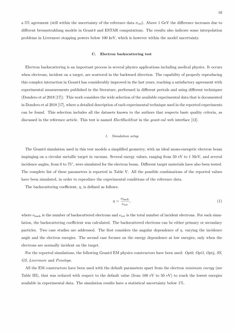
C. Electron backscattering test

Electron backscattering is an important process in several physics applications including medical physics. It occurs

when electrons, incident on a target, are scattered in the backward direction. The capability of properly reproducing

this complex interaction in Geant4 has considerably improved in the last years, reaching a satisfactory agreement with

experimental measurements published in the literature, performed in different periods and using different techniques

(Dondero et al 2018 [17]). This work considers the wide selection of the available experimental data that is documented

in Dondero et al 2018 [17], where a detailed description of each experimental technique used in the reported experiments

can be found. This selection includes all the datasets known to the authors that respects basic quality criteria, as

discussed in the reference article. This test is named ElectBackScat in the geant-val web interface [12].

1. Simulation setup

The Geant4 simulation used in this test models a simplified geometry, with an ideal mono-energetic electron beam

impinging on a circular metallic target in vacuum. Several energy values, ranging from 50 eV to 1 MeV, and several

incidence angles, from 0 to 75, were simulated for the electron beam. Different target materials have also been tested.

The complete list of these parameters is reported in Table V. All the possible combinations of the reported values

have been simulated, in order to reproduce the experimental conditions of the reference data.

The backscattering coefficient, η, is defined as follows:

η =ebacketot

, (1)

where eback is the number of backscattered electrons and etot is the total number of incident electrons. For each simu-

lation, the backscattering coefficient was calculated. The backscattered electrons can be either primary or secondary

particles. Two case studies are addressed. The first considers the angular dependence of η, varying the incidence

angle and the electron energies. The second case focuses on the energy dependence at low energies, only when the

electrons are normally incident on the target.

For the reported simulations, the following Geant4 EM physics constructors have been used: Opt0, Opt3, Opt4, SS,

GS, Livermore and Penelope.

All the EM constructors have been used with the default parameters apart from the electron minimum energy (see

Table III), that was reduced with respect to the default value (from 100 eV to 50 eV) to reach the lowest energies

available in experimental data. The simulation results have a statistical uncertainty below 1%.

11


Figure 4 shows backscattering coefficients as a function of the electron beam incident energy for an Al target for

normal incidence and for 60 incidence angle. The average number of backscattered electrons increases for larger

incidence angles. Above 0.2 MeV there is an agreement within 3 σref between experimental data and simulation

results, for all the considered EM physics constructors except GS.

At lower energies the considered experimental data show significant differences as reported in Figure 4, with a

dependence on the beam incidence angle. For normal incidence, Opt4 and SS show an agreement within 5% with

the Sandia experimental data, while Opt3 seems to underestimate the low energy backscattered electrons. GS is

comparable to Opt4 below 100 keV but then it seems to overestimate η.

In the case of a 60 incidence, all EM constructors show significant differences (within 15%) below 100 keV. After

that energy, there is an agreement between all the EM constructors and Sandia experimental data within 1-2 σref. It

is important to note that the comparison between experiments and simulations can’t be quantitatively reliable below

0.2 MeV because of the differences found in the experimental data sets themselves.

The energy-dependence results for silicon and gold targets are reported in Figure 5. Large discrepancy among

the experimental data is shown, due to different experimental conditions and measurement thresholds applied to the

scattered electrons. In general, SS, GS, Opt4, and Livermore produce results at lower energies with similar trend to

the experimental data. In particular for high Z targets the agreement with some physics constructors results can be

rather poor for energies below 10 keV. The calculation of η is influenced in the simulations, across the low energy

region, by the electron minimum energy parameter applied. This parameter is related to the physical cut-off on

the electron energy used in the experiments, that is observed to have an impact in the lowest energy η distribution

profile. Usually this cut-off ranges between 50 eV and 100 eV, due to the use of polarized grids or polarized targets,

depending on the particular experimental technique of each experiment. In Dondero et al 2018 [17] a more detailed

description of the experimental setups used in these electron backscattering measurements is reported. This cut-off

starts to influence the electron behaviour below 10 keV.

For clarity, Figures 4 and 5 show the results for a subset of tested Geant4 EM constructors. The results obtained

with Opt0 are very close to the ones generated with Opt3 as both constructors use the Urban multiple scattering

model (Ivanchenko et al 2010 [39]) in the electron energy range under study. Penelope and Livermore agree very well

with Opt4 as they use the Goudsmit-Saunderson model to simulate multiple scattering (see Section III).

In conclusion, SS, GS, Livermore, Penelope and Opt4 EM constructors show the best agreement with experimental

results. The agreement above 0.2 MeV is within 3 σref and between 5 keV and 0.2 MeV is within 15%. The agreement

between simulation and experimental data below about 5 keV is, in general, worse than at higher energies due to

differences of up to 40% for certain datasets. As discussed above, in this region the simulation results are particularly

sensitive to experiment-related parameters, like the measurement thresholds applied to the detection of scattered

electrons. Also for this reason, further investigation is still needed for electron backscattering simulation in Geant4.

12

When this process is important, caution should be used in the meantime, even using the suggested EM physics

constructors.

D. Electron forward scatter from foils at 13 and 20 MeV

The main physical processes in the transport of electrons at clinical energies are bremsstrahlung, collisional energy

loss and scattering. The components of the treatment head of a linear accelerator used for electron therapy are

intentionally thin in order to minimize energy loss and the generation of x-rays, which contaminate the treatment

beam. In this case, accurate simulation of electron scattering is paramount.

An experimental benchmark of the scatter of electrons (13 MeV and 20 MeV) is available that represents the higher

range of energies generally available in the clinic (5–25 MeV) for a comprehensive set of scattering materials (Be, C,

Al, Ti, Cu, Ta, Au) for thicknesses that result in a characteristic angle (or root mean square scattering angle) of 2–8

(Ross et al 2008 [61]). The test is called ElecForwScat in geant-val.

The benchmark gives the characteristic angle for each energy, material and thickness and the angular distribution

of fluence out to 0.9–2.5 times the characteristic angle, limited by the lateral extent of the helium bag that was placed

between the scattering foil and detector. This helium bag was used to minimize scatter of the electron beam as it passed

through this intervening space. The published measurements include a rigorous uncertainty analysis. Previously, the

Monte Carlo systems (in alphabetic order) EGS, Geant, Geant4 and PENELOPE have been benchmarked against

these measurements (Faddegon et al 2009 [18], Vilches et al 2009 [62]). It was found that the characteristic angle alone

was insufficient to quantify the discrepancy between the measurement and simulation. Thus, both the characteristic

angle and the angular distribution at points near or beyond the characteristic angle are shown. The comparison is

limited to a single, representative foil thickness, chosen to illustrate the characteristic angle closest to 5, and to

the more commonly used lower energy of 13 MeV. This is justified since any discrepancy between measurement and

calculation is expected to appear at all foil thicknesses and at both tested energies. The comparison for the angular

distribution was for representative results from a select set of scattering foils.

1. Simulation setup

A mono-energetic electron beam of 13 MeV and Gaussian circular spot of 0.1 cm FWHM was normally incident on

the exit window, a scattering foil, a monitor chamber, and mylar slabs on either side of a region filled with helium.

The foils were 0.926 g/cm2 Be, 0.546 g/cm2 C, 0.14 g/cm2 Al, 0.0910 g/cm2 Ti, 0.0864 g/cm2 Cu, 0.443 g/cm2 Ta,

and 0.0312 g/cm2 Au. The scoring plane was perpendicular to the beam axis and located 1.182 m from the exit

window. Details of the geometry along with the various scattering foil materials and thicknesses are the same as those

used in Faddegon et al 2009 [18]. The fluence of electrons was scored in radial spatial bins of 1 mm width. A two

parameter Gaussian function was fitted to the angular distribution of fluence to calculate the characteristic angle,

13

limited to the region with the fluence greater than 1/3 of the maximum value, out to a radius of 18 cm on the scoring

plane as done previously in Faddegon et al 2009 [18]. The physics constructors were Livermore, Penelope, Opt0, Opt3

and Opt4. A global production cut of 0.01 mm for secondary particles was used.


The characteristic angle from the benchmark measurement is compared with that from Geant4 in Figure 6 for all

scattering foil materials. In the top left panel, the simulation with Opt0 agrees with the measured benchmarks to

within 1 standard deviation (which is 1.0%) of the experimental uncertainty for all materials except carbon. Note

that this reasonable agreement was not seen in the fluence distributions of all the other panels, where fluence at

angles larger than the characteristic angle are shown. All the other constructors significantly underestimated the

characteristic angle of most of the foils, by up to 3% for some foils. Results for the characteristic angle calculated

with 10.5 version of Geant4 are comparable to those calculated with Geant4 9.2 (Faddegon et al 2009 [18]).

The angular distribution beyond the characteristic angle (below for the carbon foil) is shown in Figure 6 for all the

foils. Opt3 and Opt4 for Geant4 10.5 show a comparable acceptable match to the measured angular distributions

and to those calculated with the other Monte Carlo codes than past comparisons with Geant4 9.2 (Faddegon et al

2009 [18]). In general, Opt4 systematically underestimates forward-scattered electron fluence by up to 2-5% in the

MeV range. The mitigation of these differences remains as an open problem.

E. Bremsstrahlung from thick targets

The measured yield of bremsstrahlung from electrons normally incident on thick targets at radiotherapy energies as a

function of target material, electron energy, and angle provides a key benchmark for the modelling of linear accelerator

treatment heads since this requires accurate simulation of both electron scatter and bremsstrahlung within the target.

The benchmark reference dataset are the measured photon fluence per incident electron and differential in energy:

1) along the axis for 10–30 MV x-ray beams from thick targets of aluminum and lead, and 2) from 0-90 of 15 MV

beams from thick targets of beryllium, aluminum and lead. Photon fluence per unit energy per incident electron, and

total photon fluence, integrated over energy, per incident electron was experimentally determined at 1 m from the

target. Bremsstrahlung yield from 0.22 MeV to the incident electron energy was measured on the axis of 10.09, 15.18,

20.28, 25.38, and 30.45 MeV electron beams (Faddegon et al 1990 [63]). In a separate experiment, bremsstrahlung

yield down to 0.145 MeV was measured at angles out to 90 for 15.18 MeV electrons (Faddegon et al 1991 [64]). The

published measurements include a rigorous uncertainty analysis. Several Monte Carlo systems have been previously

benchmarked against these measurements (Faddegon et al 2008 [19]). This benchmark is available in the geant-val

web interface [12] with the name Bremsstrahlung.

14

1. Simulation setup

The sources in the simulation were mono-energetic, normally incident 0.35 cm diameter beams of constant fluence

with energies of 10, 15, 20, 25 and 30 MeV. The beam first impinges on a titanium exit window, followed by a silicon

transmission current monitor, then a pure target encased in a steel target chamber. Separate simulations were done

for the 15.18 MeV beam with and without the target chamber, as the chamber was not included in measurements for

angles over 10. Details of the simulation geometry are described in Faddegon et al 2008 [19]. Photon fluence was

scored on the surface of several concentric spherical rings in a sphere of 1 m radius centered at the intersection of the

beam axis with the upstream face of the target. The rings covered 1 in the polar angle and the full 0 − 360 in the

zenithal angle. Photons with energies larger than 0.22 MeV for the forward-directed benchmarks and 0.145 MeV for

the angular distribution benchmarks were scored in 100 log spaced bins and compared with the published experimental

benchmarks (Faddegon et al 1990 [63], Faddegon et al 1991 [64]).

The tested physics constructors were Penelope, Livermore, Opt0 and Opt4. A global production cut of 0.01 mm

for secondary particles was used.


Figure 7 shows selected results of the angular and spectrum distributions for beryllium (top), aluminum (middle)

and lead (bottom) for all Geant4 EM physics constructors. These results, obtained with Geant4 10.5, are in better

agreement with measurement than Geant4 9.0 patch01, where some yields were well outside 1 standard deviation of

experimental uncertainty (see results reported in Faddegon et al 2008[19]). In particular, the results obtained with

Opt3 and Opt4 agree within 1 standard deviation experimental uncertainties for all energies and all angles below

60 with the exception of the 10 MeV yield for Opt4 on the beam axis, which is just outside 1 standard deviation.

At 90 for the Al and Pb targets and 60 for the Pb target, the simulated results exceed the measurement by 1-2

standard deviations for all options, a larger discrepancy than found previously, but in better agreement with EGSnrc

and PENELOPE. The energy spectra are within 1-2 standard deviations as shown in Figure 7 except at low energy

fluence where contributions of experimental artifacts to the uncertainty may be underestimated.

F. Fano Cavity test to verify the multiple scattering and boundary crossing algorithm

This test is released as an extended example of Geant4 with the name FanoCavity. It is based on Poon et al

2005 [65] and Kawrakow 2000 [66]. It was designed to check the accuracy of the condensed history electron transport,

especially the stability of the related stepping algorithms with respect to increasing values of the maximum allowed

energy loss along an individual electron step. In case of Geant4, the corresponding continuous step limit parameter is

the dRoverRange which is the maximum allowed step length in units of fraction of the (charged) particle range. This

test is available under the name FanoCavity in the geant-val web interface [12].

15

1. Simulation setup

The different factors involved in the electron transport, i.e., the step limitation, effects of energy loss, modelling of

multiple Coulomb scattering, are tested using the Fano cavity principle described in Fano 1954 [67].

The model of ionization chamber used is the one described in Poon et al 2005 [65]: a cylinder made of 5 mm water

(G4 WATER) walls and a 2 mm cavity filled with steam (G4 WATER with a density of 1.0 mg/cm3). A beam of

1.25 MeV gamma rays parallel to the cylinder axis traverses it. With this setup, under idealized conditions, the ratio

of the dose deposited divided by the beam energy fluence must be equal to the mass-energy transfer coefficient of the

wall material.

The needed equilibrium condition for charged particles is realized using the beam regeneration after each Comp-

ton interaction: the scattered photon is reset to its initial state, energy and direction after the Compton process.

Consequently, interactions are uniformly distributed within the wall material.

It is important to mention, that unlike the other tests used in this benchmark, the Fano cavity test requires its special

physics modelling conditions. Therefore, the test fully relies on custom, local to the test EM physics constructors with

special models for ionization and Compton scattering. Ionization is simulated using a model similar to the standard

G4MollerBhabha (see the Geant4 Physics Reference Manual [28] for details) with the density dependent correction

term of the corresponding stopping power removed. Moreover, in order to have the same stopping power both in the

wall and cavity, the bremsstrahlung process is not modelled. The special model for Compton scattering guarantees

the conservation of the charged particle fluence by utilising the above mentioned beam regeneration.

To speed up the simulation it is possible to increase the Compton cross section and the secondary particles that

have no chance of reaching the cavity (when the range is smaller than 0.8 times the distance to the cavity) are killed.

To prevent the generation of δ-rays, the global production cut is set to 10 km, in order to be in the Continuous

Slowing Down Approximation. On top of these options, the finalRange (see Table III) of the energy loss is set to

10 µm, which corresponds to a kinetic energy of 20 keV in water.

As it was already mentioned, this test was designed to check the accuracy of the condensed history electron transport.

Therefore, five different local physics lists were used in the benchmark all with exactly the same special description

of the physics interactions except the Coulomb scattering. The Coulomb scattering was modelled exactly as in the

Opt0, GS, Opt3, Opt4 and WVI constructors in case of Opt0 ∗, GS∗, Opt3 ∗, Opt4 ∗ and WVI ∗, respectively. The ∗

is used in the notations in order to clearly indicate that the physics constructors used in this test are not identical to

the corresponding Geant4 EM physics constructors except the modelling of the electron Coulomb scattering and the

corresponding stepping algorithm.

16


Figure 8 shows the dependency of the ratio of the simulated dose and the theoretical one as a function of the

dRoverRange parameter value for different physics constructors discussed in the previous section.

Opt0 and GS constructors utilise the Urban (Ivanchenko et al 2010 [39]) and the Goudsmit-Saunderson (Incerti et

al 2018 [38]) models, respectively, to simulate multiple Coulomb scattering of electrons (below 100 MeV) with their

special settings recommended for high energy physics (HEP) simulation applications. The corresponding settings

include looser stepping algorithms since HEP applications, in general, are more tolerant of mistakes in the electron

stepping especially when it comes with a significantly increased computing performance. As it is expected, both

local physics constructors Opt0∗ and GS∗ show a strong dependence on the dRoverRange. Opt0 ∗ and GS∗ show

a deviation from the theoretical data values between approximately 1% and 7%, depending on the value of the

dRoverRange. The same two multiple scattering models are used to describe the Coulomb scattering in Opt3∗ (Urban)

and Opt4∗ (Goudsmit-Saunderson) but with their more accurate settings, including the stepping algorithm, that are

recommended for precision in critical applications. Accordingly, both multiple scattering models show significantly

better stability under these settings. Opt3 ∗ shows an agreement between 1% and 2%, depending on the value of the

dRoverRange. For the default value of the dRoverRange (0.2) (see dRoverRange for electrons and positrons in Table

III), the agreement is approximately 0.3%. Opt4∗ provides a remarkably small (< 0.2%) deviation from the theoretical

dose value practically independently from the dRoverRange parameter value. In addition to Opt4∗, that contains the

Goudsmit-Saunderson multiple scattering model with its most accurate configuration (Incerti et al 2018 [38]), the

WV I∗ constructor, that utilises the so called mixed-simulation description of Coulomb scattering, also provides a

high level of accuracy and stability (< 0.2%). These results are in a perfect agreement with the findings described in

a recent study (Simiele et al 2018 [68]), in which a maximum deviation from the theoretical dose values of 0.16% was

reported when the Goudsmit-Saunderson model with its Opt4∗ settings were used. Therefore, this test shows that

Geant4 can transport electrons accurately without the need of applying significant step-size reduction, and irrespective

of dRoverRange when using the Opt4 constructor, in the geometrical set-up considered (Simiele et al 2018 [68]). The

Fano test subject of this section could be repeated by including photon transport and secondary particle production

for completeness. It is recommended to repeat the test in the user’s geometry of interest.

G. Low energy electron Dose Point Kernels

The simulation of radial energy deposition profiles from isotropic sources of electrons has proven to be a useful

method of evaluating the performance of Monte Carlo codes used in medical physics, in particular for the usage of

radionuclides in targeted cancer therapy (Prestwich et al 1989 [69], Simpkin et al 1990 [70]). Although experimental

data on electron Dose Point Kernels (DPK) in liquid water - the main component of biological medium - currently do

not exist, preventing a full validation, we propose a benchmark comparing Geant4 performance to the EGSnrc Monte

17

Carlo code. This application code can be found in Geant4 as the TestEm12 extended electromagnetic example. The

test has the name LowEElectDPK in the geant-val web interface [12].

1. Simulation setup

In this setup electrons are emitted isotropically into a 4π solid angle from a point source placed in a spherical liquid

water (defined as G4 WATER) volume. In this work, results are presented for 10, 15, 100 and 1000 keV incident

monoenergetic electrons. At each simulation step, the energy deposition is randomly distributed along the step;

the radial distribution of energy deposition from the emission point is then recorded in a histogram with a weight

equal to the energy deposition value collected in the step. Radius values are scaled to the Continuous Slowing Down

Approximation (CSDA) range (r0) of the electron at the selected incident energy (E0). The DPK distribution is then

normalized to the number of incident electrons, to the selected histogram bin width and to the incident kinetic energy

value. Results are presented for 105 incident electrons. The simulation results have a statistical uncertainty lower

than 3%. Opt0, Opt3, Opt4, Livermore and Penelope have been adopted to describe the EM physics interactions. In

addition, a maximum step size equal to the bin width of the histogram is applied to control the spatial accuracy of

the energy deposition.


Figure 9 presents the scaled DPK distributions obtained for each incident electron energy using the Geant4 elec-

tromagnetic physics constructors. The curve obtained with Opt0 is not shown as this constructor produces the same

results of Opt3. These profiles are compared to EGSnrc predictions (Mainegra-Hing et al 2005 [71], computed as

described in the PhD thesis of Perrot [72]). In this comparison with EGSnrc, energy loss fluctuations have not

been considered in the simulations. All Geant4 EM physics constructors produce similar profiles as a function of

scaled radius and incident energy. Opt3 shows lower maxima at 10, 15 and 100 keV and larger profiles below about

(r/r0) = 0.4 than the EGSnrc simulation data.

In the case of Opt4, Livermore and Penelope constructors, one can observe a better agreement (within approximately

3%, corresponding to the statistical uncertaity of the Geant4 simulation results) with EGSnrc simulation data at all

incident energies, thanks to the Goudsmit-Saunderson (GS) multiple scattering model (Incerti et al 2018a [38]), which

has been recently introduced in those three physics constructors (in Geant4 version 10.5, as the best alternative to

the G4UrbanMscModel). This agreement is obtained under the condition that energy loss fluctuations are ignored in

Geant4. Indeed, EGSnrc simulation data do not take into account these fluctuations. Such agreement is not observed

when energy loss fluctuations are taken into account in the Geant4 simulations (data not shown). This underlines

that, under this condition, the GS model used in the three above constructors is able to perform as EGSnrc and can

provide more accurate simulation data. It remains however impossible to fully validate such simulations in the absence

18

of experimental data in liquid water in this energy range. At higher incident electron energies, effects of energy loss

fluctuations are not important and Geant4 Opt4 with GS model and EGSnrc results agree well, so it is possible to

conclude that both simulation tools (on the one hand Geant4 Opt4 constructor with GS model, and EGSnrc on the

other hand) can be regarded as a gold standard for such simulations.

We show in this study the full benefit of the newly implemented GS model for the simulation of electron multiple

scattering in liquid water, when compared to EGSnrc Monte Carlo code.

H. Microdosimetry test

1. Introduction

Microdosimetric spectra of lineal energy (or specific energy) are historically being used for describing radiation

quality (see ICRU Reports 40 [73] and 36 [74]), and many theoretical estimates of the Relative Biological Effectiveness

(RBE) of therapeutic beams are based on such calculations (Amols et al 1986 [75], Lindborg et al 2013 [76]).

The use of the Monte Carlo method for the calculation of stochastic energy deposition in an irradiated volume is

facilitated by the use of condensed-history models in order to reduce simulation time, especially when we are dealing

with radiotherapeutic energies. A dedicated example available in the Geant4 extended examples, called microyz, offers

a way to calculate microdosimetric spectra in liquid water target spheres.

Systematic studies of the microdosimetric performance of the low-energy condensed-history models available in

Geant4 (i.e., Livermore and Penelope) and the track structure models available in Geant4-DNA ( Incerti et al

2018b [77], Bernal et al 2015 [78], Incerti et al 2010a [79], Incerti et al 2010b [80]) have been recently carried

out for submicron volumes for the energy range 50 eV—10 keV (Kyriakou et al 2017 [20], Lazarakis et al 2018 [81],

Kyriakou et al 2019 [82]). Here we investigate the microdosimetric performance of the Opt4 constructor at energies

of radiotherapeutic interest (10 keV – 1 MeV) in terms of calculating the frequency-mean lineal energy in liquid water

spheres with a diameter of 1 µm (ICRU sphere). This test has been included in the G4-Med benchmarking system

for regression testing purposes only. The test has the name microyz in the geant-val web interface [12].

2. Simulation setup

The extended example microyz was used to calculate the probability density function of lineal energy by scoring

the energy deposited by monoenergetic electrons within target spheres of liquid water (1 µm diameter) randomly

overlapping their track. The procedure of scoring the energy deposition is provided in detail in Kyriakou et al

2017 [20]. For all simulations the global production cut was set equal to the tracking cut.

The effect of the step-size limit and tracking cut is also investigated. To obtain a statistical uncertainty below 1–2%

the number of electron tracks simulated was 106 for electron energies up to 100 keV and 105 above 100 keV.

19


Figure 10 presents the frequency-mean lineal energy as a function of incident energy for 10, 50, 100, 500 and 1000 keV

electrons using two different values for the tracking cut, 100 eV and the commonly used value in condensed-history

simulations of 1 keV.

Results are presented for three different step-size limits (called SL in the Figure), the default step-size limit which

for this test is equal to 1 mm, a step-size limit equal to the sphere diameter (1 µm), and a small step-size limit equal

to 1/10 the sphere diameter (100 nm).

We observe that for both values of the tracking cut (1 keV and 100 eV), the default step-size limit (equal to 1 mm in

the present energy range) results in a significant overestimation that increases with electron energy (at 1 MeV incident

electron energy it reaches a factor of 6 for the 100 eV cut, and a factor of 26 for the 1 keV cut). A step-size limit

equal to the sphere diameter (1 µm) also results in sizeable overestimation (20–30% for 100 eV cut and 30–50% for

1 keV cut) compared to the small step-size limit. The influence of the tracking cut is reduced when smaller step-size

limits are chosen. For example, with the small step-size limit examined (100 nm), decreasing the tracking cut from

1 keV to 100 eV affects the frequency-mean lineal energy by less than 7%.

The test microyz assumes by design discrete simulation, that is, each individual interaction leading to any modifica-

tion of the particle trajectory (energy, direction) is modelled explicitly as point-like interaction and is recorded during

the simulation. This assumption is broken when employing the Condensed History (CH) simulation technique which

leads to the observed sensitivity to the CH step size. The extent of this artificial step size dependence is determined by

the relation of the step size distribution to the size of the target sphere. Reducing this step size dependence requires

that several steps are done by electrons inside the scoring sphere which may be achieved by defining a step-size limit

less than the scoring sphere diamensions. For the commonly used tracking cuts studied in the present work (100 eV

to 1 keV), a safe value for the step-size limit is equal to the 1/10 of sphere diameter.

I. Brachytherapy test

The Brachytherapy Geant4 advanced example is used to calculate the dose rate distribution of a high dose rate

brachytherapy 192Ir source in water. We compared the results of the simulation to the reference data published in

Granero et al 2006 [83], which were obtained with Geant4 version 7.1. Therefore, the test has a regression testing

focus and is available in the geant-val interface [12] with the name Brachy-Ir.

1. Simulation setup

The 192Ir Flexisource, described in Granero et al 2006 [83], has been modelled in the center of a water box (modelled

as G4 WATER) with 30 cm size. The photon radiation field, detailed in Granero et al 2006 [83], is emitted from the

iridium radioactive core. Opt0, Opt3, Opt4, Livermore and Penelope have been tested. A global production cut was

20

fixed equal to 0.05 mm. A Geant4 scoring mesh was defined to calculate the energy deposition in the plane containing

the source. The plane is subdivided in voxels with size equal to 0.25 mm along x, y and z. 109 histories were simulated

to obtain a statistical uncertainty of 1.5% in the results. The same statistical uncertainty affects the reference data

(Granero et al 2006 [83]).


Figure 11 shows the radial dose rate distribution about an 192Ir brachytherapy source, as a measure of the energy

deposition per unit of mass, along the transverse axis of the source, 90 from the source axis.

As it can be observed in Figure 11, the simulation results obtained with any Geant4 EM constructor agree with

the reference within the uncertainty of the simulation data σref (1.5%), for almost all points, up to a distance of 8 cm

from the radioactive core. At 10 cm depth the agreement between Geant4 results and the reference data is within 3%

(corresponding to 2 σref) for all the EM constructors. No recommendation to use any of the EM constructors can be

done at this stage with this test, because the reference data are derived from Geant4 as well (Geant4 7.1).

J. Monoenergetic x-ray internal breast dosimetry test

An accurate and controlled evaluation of the radiation dose delivered during x-ray-based breast imaging is part

of quality control procedures (Perry et al 2006 [84]) and necessary for risk estimation (Dance et al 2016 [85]). This

simulation aims to compare the radiation dose predicted by means of Geant4 and experimental measurements per-

formed at the SYRMEP beamline of the ELETTRA synchrotron light source (Trieste, Italy). Dose measurements

were performed using thermoluminescent dosimeters, TLD-100H (ThermoFisher Scientific, Waltham, MA, USA), in

absolute terms and down to the local deposition level, in a mammographic acquisition setup installed at the SYRMEP

beamline (see Castelli et al 2011 [86]). The test has the name Mammo in the geant-val interface [12]. Details about

the test and the experimental procedure can be found in Fedon et al 2018a [21] and 2018b [22].

1. Simulation setup

The geometry implemented in the simulation is shown in Figure 12. A homogeneous semi-cylindrical breast phantom

(with the dimensions of 18 cm × 10 cm) consisting of four 1 cm-thick slabs was positioned within the plates of the

compression system. The phantom (CIRS Inc.,Norfolk, VA, USA) reproduces the x-ray attenuation property of a

breast with a 50% adipose and 50% fibroglandular tissue composition. Monoenergetic, parallel 20 keV photons are

emitted from a rectangular, planar x-ray source (20 cm × 12 cm) towards the breast phantom. This source geometry

models the monoenergetic nature of the SYRMEP beamline of the ELETTRA synchrotron when the double-crystal

Si monochromator is set to 20 keV. The scored physical quantity in the simulation was the dose deposited in thirty

sensitive volumes (i.e. each TLD) positioned on the xy phantom plane at four different phantom depths (i.e. the

21

scoring planes shown in Figure 12). The TLDs were modeled in terms of physical dimensions (i.e. 3.2 mm × 3.2 mm

× 0.38 mm) and relative chemical composition ( 99.5% LiF, 0.2% Mg, 0.004% Cu and 0.296% P) according to the

manufacturer. For each simulation, 2× 109 photons were simulated to obtain a statistical uncertainty lower than 1%

in all the scored quantities, estimated using the method of Sempau et al 2001 [87]. The experimental TLD procedure

and the uncertainty analysis is described in detail in Fedon et al 2018a [21]. To normalize the photon fluence in the

simulation to that used in the experiments, a scale factor was used, defined as the ratio between the experimentally

kinetic energy released per unit mass in air (kerma) and the simulated air kerma, analytically evaluated in the Monte

Carlo simulation. The constructors Opt0, Opt3, Opt4, Livermore and Penelope were tested. A global production cut

of 0.7 mm was adopted.


Dose comparison results for the depth of 3 cm are presented on the right side of Figure 12. Data for the other

depths can be found on the geant-val web interface [12]. In general, all physics constructors produce results that

agree with each other within the combined experimental uncertainty. The mean combined uncertainty for the depth

of 3 cm is 5.7% (uncertainty range from 5% to 7.7%)(Fedon et al 2018a [21]). It should be pointed out that a

systematic bias appears to be present, since the MC data results consistently overestimated the experimental data.

This overestimation is, however, within the combined experimental uncertainty. Among the Livermore, Penelope,

Opt3 and Opt4 constructors, no clear trend is observed that can suggest the use of one over the others, since the

results are within an accuracy of 5% with only few exceptions for Opt3 (ratio plot in Figure 12). However, we

noticed that the performance of Opt0 worsens with increasing depth, confirming previously observed trend (Fedon et

al 2015 [88]). A maximum relative difference of 7.7% is observed at 3 cm depth when using this constructor (position

7 in Figure 12), whereas with the other EM constructors there is a better agreement with a largest difference of 6%.

An accuracy of 5% might be considered large for a MC benchmark. However, in the case of breast dosimetry, this

is a remarkable results considering the difficulties and inherent uncertainty in these types of measurements, where

the recommended uncertainty range ±12.5% (Fedon et al 2018a [21]). Thus, these results, within the experimental

uncertainty, can be considered a valid benchmark for this specific application.

22

IV. HADRONIC PHYSICS BENCHMARKING TESTS

Hadronic interactions are paramount in hadron therapy. In proton therapy incident protons generate a secondary

neutron field which scatters in the patient producing recoil protons, which will then deposit energy in the patient

outside the target tumor and potientally in organs at risk (Paganetti 2002 [89]). In addition, it recently became

evident that the few fragments generated in proton-tissue interactions cannot be neglected (Tommasino et al 2015 [90])

because they can affect the average Linear Energy Transfer (LET) values, thus changing the biological outcome. Such

fragments are mainly produced at the entrance in the patient where the energy of the protons is higher (Tommasino

et al 2015 [90]).

In carbon ion therapy, a beam with an initial energy of 400 MeV/u, will have approximately 70% of the initial

carbon ion beam undergo fragmentation before reaching the tumor target. Such fragments contribute to the dose

in-field and are responsible for the dose delivered out-of-field, i.e. laterally to the beam and beyond the Bragg peak

(Bohlen et al 2010 [91]). The total contribution to the dose is approximately 30% for a carbon ion spread out Bragg

peak with a maximum energy of 290 MeV/u. It is therefore crucial to benchmark the hadronic physics component of

Geant4, which is often used as Monte Carlo code for hadron therapy. An accurate description of the same physical

interactions is important for radiation protection studies as well.

This section describes tests in G4-Med where only hadronic physics processes and models are tested and the

electromagnetic physics is not considered in the simulation (Section V is dedicated instead to tests which activate

both the electromagnetic and the hadronic physics). The tests described in both sections (here and Section V) were

performed in the energy range of interest for hadron therapy.

The test of section IV A benchmarks the total hadronic inelastic cross section, which is described with the Glauber-

Gribov model in Geant4 (see the Geant4 Physics Reference Manual [28]) against experimental measurements.

The tests subject of sections IV B and IV C benchmark different hadronic ion inelastic scattering constructors

G4IonBinaryCascade, G4IonQMDPhysics and G4IonINCLXXPhysics, to describe the final state of carbon ion

hadronic inelastic interactions. Table VII summarises the main features of the three constructors modelling ion frag-

mentation under study. It is important to note that the constructors adopt the same total inelastic cross section based

on the Glauber-Gribov model, while providing different descriptions of the final state of the interactions (yield, energy

and angular distributions of the secondary particles). The three constructors handle the interactions of deuteron,

triton, alpha particle, 3He and heavier nuclei.

G4IonBinaryCascade (BIC ) activates the LightIonBinaryCascade, which describes the interaction between a pro-

jectile and a single nucleon of the target nucleus interacting in the overlap region as Gaussian wave functions (Folger

et al 2004 [92]).

G4IonQMDPhysics activates the Quantum Molecular Dynamics (QMD) model. In this case all nucleons of the

target and projectile have their own wave function (Koi et al 2010 [93]).

G4IonINCLXXPhysics uses the approach of the Liege intranuclear-cascade model called here INCL (Boudard et

23

al 2013 [94], Mancusi et al 2014 [95]). The target nucleons are treated as a free Fermi gas in a static potential well,

whereas the projectile is modelled without Fermi motion. As result of this asymmetric treatment, the projectiles

which can be modelled with INCL are limited to mass numbers less than A=19; otherwise, when the target mass is

below A=19, target and projectile are interchanged internally and when both mass numbers are above A=19, the

fragmentation interaction is modelled with BIC.

In the high energy range, all the ion hadronic inelastic scattering constructors adopt the Fritiof parton string model

(FTF ) (Yarba et al 2012 [96]). In the energy overlap region (see Table VII), an interpolation between the two models

is done.

A. Test of Nucleus-Nucleus hadronic inelastic scattering cross sections

This test calculates the total cross section of hadron-nucleus and nucleus-nucleus collisions. The cross sections

are then compared to reference experimental measurements publicly available in the Experimental Nuclear Reaction

Data (EXFOR) database (Zerkin et al 2018 [97]). EXFOR provides libraries containing an extensive compilation of

experimental nuclear reaction data.

The total inelastic scattering hadronic cross sections are calculated for incident protons and carbon nuclei. The

test was named NucNucInelXS in the geant-val web interface [12].

1. Simulation setup

The benchmark test retrieves the total hadron-nucleus and nucleus-nucleus inelastic cross sections, which are stored

in a data table via the use of the class G4HadronicProcessStore in the initialisation phase of the simulation. The data

table is then compared to the reference data. Only the Geant4 prebuilt physics list QGSP BIC was benchmarked

in this test as the total inelastic hadronic cross section in all the hadronic physics constructors, used in any pre-

build Geant4 physics list, are based on the Glauber representation with the Gribov screening correction on inelastic

screening (GG model) (Kopeliovich 2003 [98], Fesefeldt 1985 [99], Grichine 2010 [100]).

The total inelastic scattering cross sections of p+126 C, p+16

8 O, p+2713Al, p+40

20Ca, 126 C+12

6 C, and 126 C+27

13Al are com-

pared with the experimental data available in EXFOR. Such reactions were selected because of relevance for hadron

therapy and because EXFOR provided an adequate number of reference experimental data.


Figure 13 shows the total inelastic cross sections calculated by means of the QGSP BIC, as a function of the

kinetic energy of the projectile, compared to the experimental data of the EXFOR database. Overall, for both

incident protons and carbon ions, an agreement within 10% was observed for most of the incident projectile energies.

Significant differences (20%-40%) were found for proton energies below 2 MeV in the case of a carbon target. These

24

differences are caused by the large variations in the experimental inelastic cross sections for p+12C, likely due to

resonances that enhance the cross section, particularly near 10.5 MeV proton energy (e.g. Dyer et al 1981 [101],

Davids et al 1971 [102]). These variations will tend to arise for low energy proton induced reactions, particularly for

light targets where the density of states is low. In the case of 12C+27Al, the data were consistently overestimated of

about 10%. This reaction should be further investigated.

25

B. 62 MeV/u 12C fragmentation test

This test concerns the nuclear interaction models available in Geant4 for low energy carbon ions. The name of the

test is LowEC12Frag in the geant-val web interface [12]. The models were benchmarked against double-differential

cross sections of the secondary fragments produced in the 12C fragmentation at 62 MeV/u on a thin carbon target.

This dataset has been acquired from De Napoli et al 2012 [103].

1. Simulation setup

As described before, the two models available in Geant4 at low energy are the Binary Light Ions Cascade (BIC )

(Folger et al 2004 [92]) and the Liege Intranuclear Cascade (INCL) (Boudard et al 2013 [94], Mancusi et al 2014 [95]).

There is a third model available in Geant4 to simulate the first part of a nuclear interaction, namely, the Quantum

Molecular Dynamics (QMD) (Koi et al 2010 [93]). However, QMD has, in its default physics constructor class

(G4IonQMDPhysics), a lower energy threshold at 100 MeV/u. Below this threshold it uses BIC. Therefore, in this

test, we decided not to benchmark the QMD model. This selfsame benchmark with QMD included, performed with

Geant4 9.4.p01, can be found in Mancini et al 2018 [23].

In order to reduce the computation time, all interactions but the hadronic inelastic ones have been switched off. All

secondaries are discarded after being produced and the target is much longer than the hadronic inelastic interaction

length. In this way, all primaries undergo an inelastic interaction, which is also the only process simulated. Secondaries

are saved immediately after being produced and the event interrupted. Data are selected to match the geometrical

acceptance and the energy resolution of the experiment. The obtained spectra are scaled by the total inelastic cross

section.


Figure 14 shows the comparison of the double-differential cross sections of α-particles production at different

emission angles.

BIC shows a doubly peaked structure. The one at higher energy is due to the fragment produced in the statistical

de-excitation of the projectile remnant, while the lower energy one comes from the de-excitation of the target. BIC

underestimates the formation of fragments in the mid-rapidity region, here at roughly 30 MeV/u of kinetic energy of

the emitted fragment, by up to one order of magnitude at small angles. Its minimum is approximately two decades

smaller than the two neighbours regions at all angles, while the projectile-like and target-like fragments formation

is overestimated for all angles. A possible explanation could be that BIC approach is based on a time-invariant

optical potential and this leads to an underestimation of the formation of a neck fragmentation events (Colonna et al

1995 [104], Toro et al 2006 [105]) in the overlapping region, roughly at mid-rapidity in semi-central reactions. On the

contrary, INCL shows a single distribution peaked at lower energy, with respect to the experimental peak. The INCL

26

predictions overestimate by around a factor ten the production of α-particles below 62 MeV/u but are compatible

with the experimental data for particles produced with higher kinetic energy. This could be due to its complete-fusion

model.

Here we show only the plot with the comparison of the α-particle production. All other plots, with the different

fragments, can be found at the geant-val web interface [12].

In conclusion, the results show that both of the tested models, BIC and INCL, exhibit limitations in reproducing

doubly differential cross sections of fragments produced in the interaction of 12C with a thin carbon target. Efforts

are underway to interface new models to Geant4 dedicated to nuclear interactions below 100 MeV/u (Mancini et al.

2019 [106] and Ciardiello et al. 2020 [107]).

C. 300 MeV/u 12C ion charge-changing cross section test

The goal of this test is to validate the partial and total charge-changing cross sections of 12C ions with energy

300 MeV/u as simulated by Geant4 against experimental data published in the literature by Toshito et al 2007 [24],

obtained with an emulsion plate in the NIRS P152 experiment. The test is named C12FragCC in the geant-val web

interface [12].

The partial charge-changing cross section to B, Be and Li fragments is about (428±21) mb, while the total is

(1183±52) mb (including the production of B, Be, H, He, Li, N, O, α, deuteron, proton, neutron and triton),

accounting for approximately 36% with respect to the other ion species in the experiment. Therefore, a correct

modelling of the carbon charge-changing process is needed for an accurate calculation of the dose in carbon ion

therapy, especially out-of-field where organs at risk may be located, the LET and the radiobiological effectiveness

(RBE).

1. Simulation setup

In this simulation, all electromagnetic processes and decay physics are switched off and only hadron and ion

transport processes are used to retrieve the carbon ion charge-changing cross section. The target geometry is a cubic

water phantom with a 10 m length. The water is defined as G4 WATER in the Geant4 simulation. Carbon ions are

irradiated from the surface of the phantom.

Only projectile-like fragments were considered in this work. Target-like fragments are also important to the dose,

however it is difficult to measure their cross section in an experiment. When an interaction occurs in the simulation,

the distance from the initial point to the interaction point is summed up as the track length only for projectile-like

fragments which can be identified as they travel to the forward region (momentum along the initiated direction >

600 MeV/c/u).

The partial cross sections of B, Be and Li isotopes were calculated by means of the simulation. This choice was

27

dictated by the availability of experimental data in Toshito et al 2007 [24].


The results of the test are shown in Figure 15 and summarised in Table VIII. The partial cross sections calculated by

means of the G4IonQMDPhysics of B, Be and Li isotopes are 144.1, 77.90 and 97.66 mb, respectively. An agreement

within the uncertainty of the reference data was observed for the total 12C charge-changing cross section and for the

Li isotope partial cross section. Differences of approximately 18% and 34% were found for the production of Be and

B isotopes, respectively. The isotope production cross sections have a similar trend when substituting QMD with

either BIC or INCL. The total fragmentation cross section is almost the same for all the ion physics constructors.

V. ELECTROMAGNETIC AND HADRONIC PHYSICS BENCHMARKING TESTS

The tests included in this section activate both electromagnetic and hadronic physics processes, using pre-built

Geant4 physics lists. QGSP BIC HP, QGSP BERT HP and QGSP BIC EMY were tested for the application of

Geant4 in proton therapy. Details of those physics lists are reported below in the energy range of interest for proton

therapy and summarised in Table IX.

In HadronElasticPhysics elastic hadronic scattering of protons and neutrons is modelled by means of the CHIPS

model (Kossov et al 2002 [108]). Below an energy of 20 MeV, the High Precision (HP) data libraries are used to

model the neutron elastic scattering. For deuteron, triton and α particles the elastic scattering model is based on

the Geant3/GHEISHA approach (Fesefeldt 1985 [99]). In both QGSP BIC HP and QGSP BIC EMY the ion elastic

scattering is modelled. The cross section is calculated with the Glauber-Gribov model while the diffuse model describes

the final state (documented in Grichine 2010 [109]).

In QGSP BIC HP and QGSP BIC EMY the hadronic inelastic scattering of incident neutrons and protons on

nucleons of the target nuclei is described by means of the Binary Intranuclear Cascade (BIC in Table IX) model, below

approximately 10 GeV (Folger et al 2004 [92]). The BIC is followed by the Geant4 Precompound model describing the

de-excitation of the remnant nucleus (Allison et al 2016 [3]). This is followed in turn by the evaporation of particles

until the nucleus is fully de-excited (see the Geant4 Physics Reference Manual [28]). In QGSP BERT HP the proton

and neutron inelastic scattering is described with the Bertini model (Wright et al 2015 [110]), which has its own

precompound and evaporation models.

In all the investigated physics lists, the LightIonBinaryCascade describes the intranuclear cascade of deuteron,

triton, He isotopes and heavier nuclei (Allison et al 2016 [3]). Also in this case the cascade is followed by the de-

excitation of the remnant nucleus via the Precompound model and the nuclear evaporation (Allison et al 2016 [3]). HP

(see Table IX) means that neutron inelastic scattering, capture and fission are modelled using the HP data libraries

below 20 MeV. Particle decay is modelled in the physics lists under study. The radioactive decay is activated by

28

default in the QGSP BIC HP and QGSP BIC EMY, while it is not included in the QGSP BERT HP.

A. 67.5 MeV Proton Bragg curves in water

The accurate calculation of the proton range is essential in Monte Carlo calculations for proton therapy. While

submillimeter accuracy in-depth penetration can be achieved by fine tuning of the proton energy, depth-dose curves

measured from a proton beam with an energy accurately known are desirable for benchmarking purposes. In this test,

the setup for comparing Monte Carlo calculated Bragg peaks with experimental data of submillimeter (< 0.2 mm)

uncertainty is described. The test is available in the geant-val web interface [12] with the name LowEProtonBraggBeak.

1. Simulation setup

A 67.5 MeV proton beam with a Gaussian energy spread of 0.4 MeV, and a uniform 5 mm × 10 mm oval spot

travels through a tantalum (Ta) foil of either 101.6 µm or 381 µm thickness. The geometry up to and including the

water phantom is described in detail in Faddegon et al 2015 [25]. The sensitive region in the water phantom is 5 × 5

× 50 mm3 divided into 1000 slices. The depth-dose curves in water (density = 0.998 g/cm3 and ionization potential

I=78 eV [111], see Faggedon et al 2015 [25]) are calculated and then fitted with an analytical expression for the Bragg

curve described in Bortfield 1997 [112]. The fitting parameters range, R0, and spread, s, are compared against the

corresponding experimental parameters from depth-dose measurement from Faddegon et al 2015 [25]. The range, R0,

is the depth at 80% distal falloff of the Bragg curve, whereas s is the spread of a Gaussian describing the width of

the Bragg peak according to Bortfeld et al 1997 [112].

The physics list included alternatively Livermore, Penelope, Opt3 and Opt4. This test calculates the proton range

which depends on the EM physics processes only. Therefore, the hadronic physics component was modelled only by

means of the QGSP BIC HP as described in Testa et al 2013 [113], where a comprehensive validation of the Geant4

physics list for proton therapy was performed. A global production cut for secondary electrons of 50 µm was used

everywhere with exception of the beam plug region. In there, a production cut of 20 µm was used. Simulations

using the Bertini hadronic model gave the same results for the four tested EM physics constructors within statistical

uncertainty.


The left side of Figure 16 shows the depth-dose distributions in water for simulated (lines) data and measured data

(symbols). In the right side of Figure 16, the differences in Bragg peak spread (s) and range (R0) are shown in the top

and bottom of the figure, respectively. Differences in R0 were within 2 standard deviations whereas (σ) for the s were

within 1 σref, for all the EM constructors. The uncertainties shown in the figure include experimental, fitting and

29

statistical uncertainties from the Monte Carlo simulations. As depicted, the Monte Carlo calculation underestimates

R0 within 0.5 mm, and overestimates s within 0.05 mm.

In the end, the proton range and Bragg curve spread calculated with Geant4 10.05 were in acceptable agreement

with the measured depth-dose curves within better than 0.5 mm.

B. Light ion Bragg Peak curves

The accurate modeling of Bragg curves of proton and light ion beams in water is of key importance to ensure code

reliability for applications in hadron therapy. In this test, we compare our Geant4 calculations against mean range

values estimated experimentally at GSI (Schardt et al 2007 [114]) for proton and 12C beams at energies of interest in

particle therapy. The test is available in the geant-val web interface [12] under the name LightIonBraggPeak.

1. Simulation setup

The Bragg curve measurements were carried out by means of a water tank, whose thickness could be varied with

micrometric accuracy, and two ionization chambers (IC) placed upstream (IC1) and downstream (IC2) in the tank.

These measurements were carried out for protons and 12C ions, among other beam species, at various nominal energies

to provide range-in-water values roughly from 3 to 30 cm. The ratio between the ionization registered by IC2 over

that registered by IC1 was used to estimate the mean energy deposition at each depth with respect to the energy

deposited at the entrance. According to a previous work (Bichsel et al 2000 [115]), the mean range of the beam was

estimated to be at the depth where the distal edge of the Bragg curve was equal to 82% of the peak value, Rd82.

More details of the experimental setup can be found in Schardt et al 2007 [114].

For our calculations with Geant4, the geometry consisted of a simple water tank, modelled using G4 WATER

material with density corrected according to room temperature (24 C, 0.997 g/cm3). The energy deposition was

scored by means of cylindrical volumes with a radius of 28 mm (equal to the radius of the ICs) and a thickness of

50 µm (similar to the water equivalent thickness of both ICs). Pencil beams were defined in our calculations with a

mean energy equal to the reported nominal energy; the energy distribution was Gaussian, whose spread was estimated

by fitting the width of the experimental distal fall-off, defined from the 90% and 10% of the peak value. For each

type of beam, all EM models matched experimental data with the same energy spread, which FWHM was of the

order of, or below, 0.2% of the nominal energy in all cases. We tested the electromagnetic physics constructors: Opt0,

Opt3, Opt4, Livermore and Penelope; the hadronic physics was activated as defined in QGSP BIC HP physics list.

Consistent with the experimental data, we calculated the depth, at distal edge, where the energy deposition was equal

to the 82% of the maximum; this value was compared with those obtained from the experiments.

30


Figure 17 shows the absolute differences obtained in the value of Rd82 between measurements (suffix “exp”) and

Geant4 calculations (“G4”) as a function of depth in water for protons (125–200 MeV/u) and 12C beams (100–

400 MeV/u), respectively. In all cases, dose was calculated with statistical uncertainty below 1% (1σ) at the scoring

volumes around the peak of the Bragg curve to ensure a small propagation to the calculated Rd82; thus, the uncertainty

of Rd82 was estimated to be equal to the scoring volume thickness (50 µm). As for proton beams, the agreement was

better than 0.2 mm (.0.1%) in all cases, which is considered remarkable, given that (1) the precision of the algorithm

itself is within 2% and (2) particle therapy calculations require a precision of about 1 mm. As for 12C beams, on

one hand we could observe that Opt0 showed range deviations of about 1.2%–2.5%, i.e. similar to the precision of

the Bethe-Bloch model used. On the other hand, the other EM physics constructors showed deviations about three

times smaller, with a maximum absolute difference about 0.8 mm (0.3%) for the largest energy (400 MeV/u), and

maximum relative difference of 1.1% for the smaller energy (100 MeV/u). This can be explained by the fact that

the ion stopping is calculated in Opt0 by means of an algorithm based on Bethe-Bloch formula, whereas in the other

constructors a more precise method is implemented, based on a parameterization of stopping power values published

by the ICRU (Sigmund et al 2009 [35]) for some ions and materials, as described in Lechner et al 2010 [116].

In summary, all electromagnetic physics constructors are able to successfully model the stopping of protons in water,

whereas for 12C beams only Opt3, Opt4, Livermore and Penelope are recommended.

C. Neutron yield of protons with energies 113 MeV and 256 MeV and carbon ions at 290 MeV/u

Absolute neutron yields from protons and carbon ions at therapeutic energies interacting in targets of materials

of interest for medical physics are presented. This benchmark shows the current status of two of the main Geant4

physics lists for hadronic physics used by the community in medical applications. For protons, two energies (113 MeV

and 256 MeV) have been selected, as they are important in clinical applications. The proton beams are incident on

one of three targets made of aluminum, carbon and iron, with thickness large enough to fully stop the beam. For

carbon ions of 290 MeV/u, the beam is incident on a water (G4 WATER material) phantom of 18 cm thickness.

The results of the test are available in the geant-val web interface under the name of ProtonC12NeutronYield [12].

1. Simulation setup

Experimental neutron yields from thick targets of different materials bombarded by protons of energies below

256 MeV were obtained from Meier et al 1989 [117] and 1990 [118]; for carbon ions interacting in water the data

was obtained from Satoh et al 2016 [119]. For protons, the Monte Carlo simulations modelled a cylindrical target

irradiated with a uniformly distributed, zero divergence, monoenergetic (113 MeV or 256 MeV) proton beam with a

radius equal to the radius of the target. The beam was located upstream of the target. The radius, thickness and

31

material of each target are shown in Table X.

Secondary neutrons produced in the inelastic nuclear interactions within the targets and escaped were scored at

the surface of spherical rings (radius of 90 m) that covered specific angular bins of 4 of thickness. For carbon ions, a

monoenergetic carbon ion beam of 0.25 cm radius, 290 MeV/u energy and zero divergence was simulated. The target

was a water phantom 18 cm thick. Detailed dimensions are shown in Satoh et al 2016 [119]. The neutron yield per

incident primary particle per steradian per energy (equally spaced logarithmic energy intervals) was scored at specific

angular bins. For proton beams, the neutron yield was scored at 7.5, 30, 60 and 150 for 113 MeV and at 30,

60, 120 and 150 for 256 MeV. For carbon ions, the neutron yield was scored from 15-90 at 15 angular steps.

The physics lists under study included alternatively QGSP BIC HP and QGSP BERT HP EMZ. Both adopt the

EM constructor Opt4 (indicated with the suffix EMZ in the pre-built Geant4 physics lists). A global production cut

of 0.05 mm was used.


In Figure 18, top left, representative results are shown for the absolute neutron yield for protons (incident on

aluminum) and carbon ions (on water) for several angles. Experimental data are shown with empty circles. In the

figure, the ratio between the calculated to experimental integrated yields is shown for several angles and materials. For

the carbon ion case, the yields were integrated from 2 MeV as reported in Satoh et al 2016 [119]. As shown, for protons

there exists an overall better agreement (within 2 standard deviations) between QGSP BIC HP and the experimental

yield for all the angles and materials compared to QGSP BERT HP EMZ. However, the largest differences between

the two physics lists were found at larger angles for the aluminum target. For water material, there was not significant

difference between the two physics list for all the angles. In that scenario the yields were overestimated by up to 50%.

As a comparative with other Monte Carlo engines, results from Satoh et al 2016 [119] using PHITS are shown and

they agreed with Geant4 calculation within 1 standard deviation.

In summary, a marginally closer agreement with measured data was achieved with QGSP BIC HP physics list for

high Z materials using the proton beams. For carbon ions, no statistically significant difference was found between the

two hadronic physics lists used, because they both use the same physics models to describe the hadronic interactions of

heavier ions. For the case involving carbon ions, the neutron yields were underestimated compared with experimental

data by 50% on average, and by 11% compared with published data calculated with the PHITS code.

D. Fragmentation of a 400 MeV/u 12C ion beam in water

This test, published in Bolst et al 2017 [26], benchmarks Geant4’s modelling of the fragmentation process against ex-

perimental measurements of a 12C ion beam incident upon a water target performed at GSI (Haettner et al 2013 [120]).

The measured data includes fragment yields from hydrogen to boron for different thicknesses of water irradiated by a

32

mono-energetic 400 MeV/u 12C ion pencil beam, as well as the fragment’s angular and energy distributions. The full

results of the test can be downloaded from the geant-val web interface [12]. The name of the test is FragTest.

1. Simulation setup

The simulation consists of a mono-energetic 12C ion pencil beam with an initial energy of 400 MeV/u and energy

σ of 0.15%, with a FWHM of 5 mm. The beam is incident upon a variable thickness of water with an area of 50

× 50 cm2 and thicknesses of: 59 mm, 159 mm, 258 mm, 279 mm, 288 mm, 312 mm and 347 mm. Fragments were

collected in a 2.94 m radius hemisphere centered on the water slab. For fragment yields, fragments were scored in a

10 cone from the center of the hemisphere. Fragment’s angular distributions were scored in arcs on the hemisphere

with angles of 0.4, corresponding to the size of the detector used in the experiment. The energy distributions of

fragments were calculated based on the time of flight of fragments scored in the 0.4 arcs.

Electromagnetic interactions were modelled using Opt4, with a global production cut of 10 mm for electrons,

the production cut was set this high since the electron production did not affect the production of fragments. The

QGSP BIC HP hadronic physics component was used with alternative physics models describing the hadronic inelastic

scattering of heavy ions: G4IonBinaryCascadePhysics (BIC ), G4IonQMDPhysics (QMD) and G4IonINCLXXPhysics

(INCL). All default configurations were used for all models investigated in this work.


Fragment yields scored within a 10 cone are shown in Figure 19. It can be seen that the yield varies signifi-

cantly between the fragmentation models, up to ∼20% for particular fragment species. For the lighter fragments H

and He, which represent the most abundant fragments, all alternative models agreed within ∼20% of experimental

measurements. For this particular version of Geant4 (10.5), INCL gives the best agreement with experiment for H

fragments while QMD agrees the best for the yield of He fragment. Sample angular and energy distributions are

shown in Figure 20, the simulation distributions shown here are normalised to the same area under the curve as the

experiment. This is done to compare just the distributions produced by the simulation against the experimental data.

INCL was seen to reproduce experimental angular distributions better than the other two models with the exception

of H, where QMD reproduced the best. For kinetic energy distributions, INCL was seen to perform the poorest of

the three models, with its energy distributions systematically being shifted ∼10% to lower energies compared to the

other models for most measurements. BIC and QMD were seen to perform very similarly to one another for both the

angular and energy distributions, with QMD performing slightly better out of the two. Due to different fragmentation

models giving better agreement with experimental measurements for angular and energy distributions of fragments,

the user should carefully consider their needs when selecting a model for fragmentation. The simulations were also

performed with the Geant4 EM constructor Opt3, however no significant differences were found between the two

33

compared to Opt4.

34

E. Test on cell survival curve modelling for proton therapy

This test is focused on evaluating the capability of Geant4 to reproduce in-vitro cell survival curves, also referred to

as surviving fraction (SF), against experimental measurements (Chaudary et al 2014 [121]), performed at the CATANA

facility radiating the radio-responsive prostate DU145 cells and breast cancer cell line MDA-MB-231 (Petringa et al

2019 [27]), at 20 mm depth in water, corresponding to the mid of a clinical 62 MeV modulated clinical proton beam.

The test is called Hadrontherapy in the geant-val web interface [12].

The SF is calculated with the Linear Quadratic Model:

SF (D) = e−(αD+βD2), (2)

where SF(D) is the fraction of cells surviving when delivering a dose D; α and β are constants describing the linear

and quadratic components of cell killing, respectively.

Precompiled Look-up Tables (LUTs) contain the values of αi and βi for a set of monoenergetic ions (with Z spanning

from 1 to 8). αi and βi are calculated with the the Local Effect Model, LEM (Elsasser et al 2010 [122], Friedrich et al

2012 [123]) and are tabulated as a function of the ion kinetic energy Ei and delivered dose Di in a specific voxel of the

simulated material. Ei and Di can be derived from the Geant4 simulations and then used as input of an algorithm

able to compute the average values of 〈α〉 and 〈β〉 in a mixed radiation field, interpolating the best αi and βi and

using the following weighted formulas:

〈α〉 =

∑i αi ·Di∑iDi

, (3)

〈β〉 =

(∑i

√βi ·Di∑iDi

)2

, (4)

where the index i refers to the different incident ions interacting in the voxel. This method is referred here as LEM

III-weighted method. The LUTs are created taking into account the total LET at the corresponding position of the

cell layer irradiation [124]. The input parameters of the LEM models were optimized referring to the radiobiological

results. The threshold dose was fixed to 5 and 9 Gy for the MDA-MB-231 and DU-145 respectively, the nucleus radius

was 4 µm in both cases.

35

1. Simulation setup

The experimental setup (transport beamline elements, detectors, irradiation device, etc.) used for cells irradiation

has been modelled in detail using the Hadrontherapy advanced example (Cirrone et al 2017 [125]). The source consists

of a 62 MeV proton beam characterized by a gaussian energy and angular distribution with a standard deviation of

0.3 MeV and 0.028, respectively. The beam spot size was circular, with a gaussian spatial distribution (standard

deviation of 3 mm). A plastic rotating modulator wheel (Jia et al 2016 [126]) routinely used for real treatments was

simulated for the correct reconstruction of the modulated beam (clinical Spread Out Bragg Peak or SOBP). A total

of 3.6 · 108 histories were simulated in each simulation. Dose as a function of depth is calculated in a voxelised water

phantom positioned at the end of the beam line. The water tank was divided into 400 × 400 × 0.01 mm3 segments to

reproduce the real experimental conditions. The water material is modelled with G4 WATER NIST. Dose, fluence,

dose-averaged Linear Energy Transfer (LET) of the primary proton beam and generated secondaries were calculated in

the simulations; α and β values were determined using equations 3 and 4, along with the LUTs. The QGSP BIC HP

physics list was used. The dose-averaged LET at the cells was 4.5 keV/mum. The global production cut was set to

0.01 mm.


Figure 21 shows the SF curves as derived from the experimental measurements and the Geant4 simulation.

The agreement between experimental data and Geant4 simulations data was evaluated applying the χ2 test in the

case of two independent distributions.

We obtained a χ2 value of 4.23 and 3.64 for the DU145 and MDA cell lines, respectively.

The χ2 test confirmed the good agreement between the two distributions even if, as expected, at doses greater than

3 Gy the differences become more evident (well above the 20%)[27].

VI. SUMMARY AND CONCLUSIONS

G4-Med is a group of currently 18 tests, regularly executed on the CERN computing infrastructure via the geant-val

platform, to benchmark Geant4 against reference data for medical physics applications. G4-Med can also be used for

regression testing purposes of Geant4. The results of the tests are provided to the Geant4 user community on-line via

the geant-val web interface [12].

This work was focused on the description of the tests of G4-Med and on the results of the benchmarking of

Geant4 10.5 against reference data.

Table XI is intended to provide a summary of the main results of the electromagnetic physics tests, subject of

Section III. We encourage the readers to refer to the specific tests of interest, for a more detailed analysis of the

results in specific scenarios of application of Geant4.

36

The agreement is defined based on the discussion of the results of each individual test in Section III. SS and GS

are not included in the Table as they have been used in a very limited set of tests.

In the case of the test concerning photon attenuation coefficients in water (PhotonAttenuation), slightly better

agreement with respect to reference data was found for Opt4. The test includes one material only at this stage and

we will expand it to other materials in the near future. We will also consider to extend the comparison of Geant4 to

other reference data.

The electronic stopping power test (ElectDEDX ) showed an agreement with ESTAR within the reference data

uncertainty (1 σref). This test is useful for regression testing purposes as it monitors a physical quantity important

for the calculation of energy deposition in a target.

The electron backscattering test shows an agreement with respect to the available experimental data that clearly

depends on the electron energy range and the Geant4 EM physics constructor. In particular below 5 keV the results

should be taken with caution for any constructor, including the suggested ones. The best EM physics constructors to

model the electron backscattering were found to be Opt4, SS, Livermore and Penelope.

For electron forward scatter, the angular distribution of electron fluence at 1.18 m calculated with Opt4 was

significantly underestimated (> 1 standard deviation) in comparison to experimental data for foils of higher Z than

Be by 2-5%, with calculated results comparable to or better than the comparison with the other physics constructors.

For bremsstrahlung from thick Be, Al and Pb targets at radiotherapy energies, bremsstrahlung yields (≤ 1-2 standard

deviations) were in better agreement with experimental data when using Opt3 and Opt4. For these constructors, the

differences were significant (> 1 standard deviation) at larger angles for the higher-Z targets (≥ 60).

The Fano cavity test (FanoCavity) was designed specifically to check the accuracy of the condensed history electron

transport and this test demonstrates that the Goudsmit-Saunderson (GS) multiple scattering model (included in

Opt4, Livermore and Penelope) provides a high level of accuracy and stability. Similar results were obtained for the

WVI∗ constructor.

The Dose Point Kernel test (LowEElecDPK ) demonstrates that the Opt4 constructor provides the best agreement

with the selected standard (EGSnrc). This test is currently used as a regression testing benchmark for Geant4 allowing

to verify the stability of DPK profiles along with Geant4 updates, especially when electron multiple scattering models

undergo changes or updates. It remains impossible to validate Geant4 in terms of DPK in the absence of experimental

data in water in the low electron energy range.

The results of the microdosimetry test (microyz ) demonstrate that, when using Geant4 condensed history approach

in EM simulations of electron transport in microdosimetric applications, it is important to limit the step size. It is

shown that 1/10 of the sensitive volume diameter is adequate.

The Brachytherapy test (Brachy-Ir) has a regression testing purpose. Geant4 is compared against previous sim-

ulation results in calculating the radial dose rate distribution of a 192Ir source. This test is of interest to monitor

the evolution of Geant4 and will be extended in the near future to other brachytherapy sources. We intend also to

compare the results of the simulation to dosimetric experimental measurements available in the literature.

37

The test on monoenergetic x-ray internal breast dosimetry (Mammo) showed an agreement between Geant4 and

experimental data within the experimental uncertainty. It was observed that Opt0 provided the worst performance

among the EM constructors under study.

In summary, the EM tests showed that Opt0 in general is the constructor with the least agreement with respect

to the reference data. For the other physics constructors, the results of the tests should support users to select

the appropriate EM physics constructor for their medical physics application. It was observed that Opt4 had good

agreement with the reference data for all the tests. This result was expected as this constructor was developed to

provide the most accurate Geant4 physics models, irrespective of CPU performance.

Table XII summarises the results obtained for the hadronic tests subject of section IV.

The test of Nucleus-Nucleus hadronic inelastic scattering cross sections (NucNucInelXS ) considered a limited num-

ber of projectiles of interest for hadron therapy (protons and 12C ions), incident on a limited number of targets.

The choice of targets was performed based on the availability of experimental measurements in the EXFOR data

library (Zerkin et al 2018 [97]). In general, an agreement within approximately 10% was found between Geant4 and

the experimental data for the cases under study. The next step of this test is to find more reference experimental

measurements to be able to benchmark the Geant4 inelastic scattering cross sections for more targets of interest for

medical physics applications.

The 62 MeV/u 12C fragmentation test (LowEC12Frag) showed that both the Geant4 Ion Binary Cascade and the

INCL models have limitations in reproducing doubly differential cross sections of fragments produced in the interaction

of 12C with a thin carbon target. The results of this test show a possible domain of improvement of Geant4 of interest

for carbon ion therapy.

The test on the 300 MeV/u 12C ion charge-changing cross section (C12FragCC ) demonstrated that all hadronic ion

fragmentation models, G4IonQMDPhysics (QMD), G4IonBinaryCascade(BIC ) and G4IonINCLXXPhysics(INCL),

reproduce the total and Li partial charge-changing cross sections. However, they all underestimate the reference

experimental data for Be and B fragments.

Table XIII summarises the results obtained for the hadronic tests subject of section V, where the EM constructor

is varied while keeping the hadronic physics component modelled with QGSP BIC HP.

The test modelling a 67.5 MeV proton Bragg Peak in water (LowEProtonBraggPeak) showed that Geant4 can

reproduce the Bragg peak spread within the uncertainty of the experimental measurements and the range within 0.5

mm accuracy. This result was confirmed for higher proton energies (125–200 MeV/u) by the Light Ion Bragg Curve

test (LightIonBraggPeak). In this case an agreement within 0.1% (< 0.2 mm) was observed for Rd82. In the case of

incident 100–400 MeV/u 12C ions, an agreement within 1.1% was found for all EM constructors apart from Opt0.

Table XIV summarises the results obtained for the hadronic tests subject of section V, where the EM constructor

is kept constant while changing the hadronic physics component.

The neutron yield produced by 113 MeV and 256 MeV protons showed a a marginally closer agreement when using

QGSP BIC HP rather than QGSP BERT HP.

38

The 400 MeV/u 12C ion fragmentation test (FragTest) showed that BIC and QMD produce similar yields of light

fragments (Z=1–5), with similar kinetic energy and angular distribution. Worst agreement in terms of fragments

yield was observed for INCL, however this model produces the best description in terms of angular distributions of

the fragments. The results of this test are consistent with the outcome of the charge-changing cross section test which

demonstrated a better agreement between BIC and QMD to the reference data than INCL.

The test on the cell survival curves (Hadrontherapy), of interest for ion therapy, is intended to validate Geant4

against in-vitro radiobiological measurements. In particular, surviving fraction curves calculated with Hadrontherapy

were compared with experimental data for different cell lines. A good agreement was found for low doses (up to 3

Gy), while significant discrepancies were evident at higher delivered doses. Provided the current stage of research in

in-silico radiobiological modelling (e.g. Abolfath et al 2017 [128]), the overall agreement was deemed satisfactory.

For hadron therapy, it is recommended not to use the EM constructor Opt0. The hadronic tests showed that

QGSP BIC HP physics list (which models EM interactions with Opt4 in Geant4 10.5) provides an overall adequate

description of the physics involved in hadron therapy, including proton and carbon ion therapy. However, it should be

noted that only few physical quantities (position and spread of the Bragg Peak, neutron yields, fragment yields) have

been subject of testing. New tests should be included in the next stage of the project to validate Geant4 in terms of

dosimetry against experimental measurements.

Concerning the carbon ion fragmentation tests, the results show a slightly better performance when using QMD

and BIC ion fragmentation models. The charge-changing cross section and fragmentation tests show that ion frag-

mentation modelling is a domain of possible improvement of Geant4.

In conclusion, we encourage Geant4 users to use benchmarked Geant4 physics constructors and lists. The results

presented and discussed in this paper will aid users tailoring physics lists to their particular application.

The next phase of the project will proceed in two main directions. The first one is the benchmarking of the

computing performance of the pre-built Geant4 physics constructors and lists. We will use the regression testing to

investigate the evolution of the Geant4 physics component for medical applications in terms of both accuracy and

computing performance. The second main direction will be to extend the current tests and include new ones to cover

domains which are currently not tested, e.g. x-ray radiotherapy and nuclear medicine.

ACKNOWLEDGMENTS

The authors would like to thank Krzysztof Genser and Daren Sawkey for their feedback aimed to improve the

quality of the paper.

D. Bolst acknowledges the support of the Australian Government Research Training Program Scholarship. M. A.

Cortes-Giraldo, A. Perales and J. M. Quesada acknowledge financial support from the Spanish Ministry of Economy

and Competitiveness under grant FPA2016-77689-C2-1-R.

B. Faddegon and J. Ramos-Mendez acknowledge partial financial support from the NIH grant U24CA215123.

39

D. Bolst, S. Guatelli, D. Sakata, S. Incerti and I. Kyriakou acknowledge financial support from the Australian

Research Council, ARC DP170100967.

S. Incerti acknowledges the financial support of CNRS through the IN2P3/MOVI Master Project and through the

France-Greece PICS 8235 funding scheme.

I. Kyriakou acknowledges additional financial support from the European Space Agency (Contract No.

4000126645/19/NL/BW).

E. C. Simpson acknowledges financial support from the Australian Research Council under grant DP170102423.

I. Sechopoulos and C. Fedon acknowledge financial support from the Susan G Komen Foundation for the Cure

grant IIR13262248.

[1] S. Agostinelli et al., “Geant4 −a simulation toolkit,” Nuclear Instruments and Methods in Physics Research Section A:

Accelerators, Spectrometers, Detectors and Associated Equipment, vol. 506, no. 3, pp. 250 – 303, 2003.

[2] J. Allison et al., “Geant4 developments and applications,” IEEE Transactions on Nuclear Science, vol. 53, pp. 270–278,

Feb 2006.

[3] J. Allison et al., “Recent developments in Geant4,” Nuclear Instruments and Methods in Physics Research Section A:

Accelerators, Spectrometers, Detectors and Associated Equipment, vol. 835, pp. 186 – 225, 2016.

[4] S. Guatelli and S. Incerti, “Monte carlo simulations for medical physics: From fundamental physics to cancer treatment,”

2017.

[5] L. Archambault, L. Beaulieu, J.-F. Carrier, F. Castrovillari, S. Chauvie, F. Foppiano, G. Ghiso, S. Guatelli, S. Incerti,

E. Lamanna, et al., “Overview of Geant4 applications in medical physics,” in 2003 IEEE Nuclear Science Symposium.

Conference Record (IEEE Cat. No. 03CH37515), vol. 3, pp. 1743–1745, IEEE, 2003.

[6] P. Arce, J. Ignacio Lagares, L. Harkness, D. Perez-Astudillo, M. Canadas, P. Rato, M. de Prado, Y. Abreu, G. de Lorenzo,

M. Kolstein, and A. Dıaz, “Gamos: A framework to do Geant4 simulations in different physics fields with an user-friendly

interface,” Nuclear Instruments and Methods in Physics Research Section A: Accelerators, Spectrometers, Detectors and

Associated Equipment, vol. 735, no. C, pp. 304–313, 2014.

[7] S. Jan, D. Benoit, E. Becheva, T. Carlier, F. Cassol, P. Descourt, T. Frisson, L. Grevillot, L. Guigues, L. Maigne, C. Morel,

Y. Perrot, N. Rehfeld, D. Sarrut, D. R. Schaart, S. Stute, U. Pietrzyk, D. Visvikis, N. Zahra, and I. Buvat, “GATE v6: a

major enhancement of the GATE simulation platform enabling modelling of CT and radiotherapy,” Physics in Medicine

and Biology, vol. 56, pp. 881–901, 2011.

[8] T. Akagi, T. Aso, B. Faddegon, A. Kimura, N. Matsufuji, T. Nishi, C. Omachi, H. Paganetti, J. Perl, T. Sasaki, et al., “The

ptsim and topas projects, bringing geant4 to the particle therapy clinic,” Progress in Nuclear Science and Technology,

vol. 2, pp. 912–917, 2011.

[9] T. Akagi, T. Aso, G. Iwai, A. Kimura, S. Kameoka, S. Lee, Y. Maeda, N. Matsufuji, T. Nishio, C. Omachi, et al.,

“Geant4-based particle therapy simulation framework for verification of dose distributions in proton therapy facilities,”

Prog. in Nucl. Sci. and Technol., vol. 4, pp. 896–900, 2014.

[10] J. Perl, J. Shin, J. Schumann, B. Faddegon, and H. Paganetti, “Topas: an innovative proton monte carlo platform for

40

research and clinical applications,” Medical physics, vol. 39, no. 11, pp. 6818–6837, 2012.

[11] https://twiki.cern.ch/twiki/bin/view/Geant4/G4MSBG.

[12] https://geant-val.cern.ch/layouts. geant-val web interface.

[13] https://www.geant4.org/geant4. Geant4 Collaboration web page.

[14] Freyermuth, Luc, Konstantinov, Dmitri, Latyshev, Grigorii, Razumov, Ivan, Pokorski, Witold, and Ribon, Alberto,

“Geant-val: - a web application for validation of detector simulations,” EPJ Web Conf., vol. 214, p. 05002, 2019.

[15] K. Amako, S. Guatelli, V. Ivanchenko, et al., “Validation of Geant4 electromagnetic physics versus the NIST databases,”

IEEE Trans. Nucl. Sci, vol. 52, p. 910, 2005.

[16] Note on NIST X-ray Attenuation Databases 2016, https://www.nist.gov/pml/note-nist-x-ray-attenuation-databases

[17] P. Dondero, A. Mantero, V. Ivanchencko, S. Lotti, T. Mineo, and V. Fioretti, “Electron backscattering simulation in

Geant4,” Nuclear Instruments and Methods in Physics Research Section B: Beam Interactions with Materials and Atoms,

vol. 425, pp. 18–25, 2018.

[18] B. A. Faddegon, I. Kawrakow, Y. Kubyshin, J. Perl, J. Sempau, and L. Urban, “The accuracy of egsnrc, geant4 and

penelope monte carlo systems for the simulation of electron scatter in external beam radiotherapy,” Physics in Medicine

& Biology, vol. 54, no. 20, p. 6151, 2009.

[19] B. A. Faddegon, M. Asai, J. Perl, C. Ross, J. Sempau, J. Tinslay, and F. Salvat, “Benchmarking of monte carlo simulation

of bremsstrahlung from thick targets at radiotherapy energies,” Medical physics, vol. 35, no. 10, pp. 4308–4317, 2008.

[20] I. Kyriakou, D. Emfietzoglou, V. Ivanchenko, M. C. Bordage, S. Guatelli, P. Lazarakis, H. Tran, and S. Incerti, “Micro-

dosimetry of electrons in liquid water using the low-energy models of Geant4,” Journal of Applied Physics, vol. 122, no. 2,

p. 024303, 2017.

[21] C. Fedon, M. Caballo, R. Longo, A. Trianni, and I. Sechopoulos, “Internal breast dosimetry in mammography: Experimen-

tal methods and monte carlo validation with a monoenergetic x-ray beam,” Medical physics, vol. 45, no. 4, pp. 1724–1737,

2018a.

[22] C. Fedon, M. Caballo, and I. Sechopoulos, “Internal breast dosimetry in mammography: Monte carlo validation in

homogeneous and anthropomorphic breast phantoms with a clinical mammography system,” Medical physics, vol. 45,

no. 8, pp. 3950–3961, 2018b.

[23] C. Mancini-Terracciano, B. Caccia, M. Colonna, M. De Napoli, A. Dotti, R. Faccini, P. Napolitani, L. Pandola, E. S.

Camillocci, G. Traini, et al., “Validation of Geant4 nuclear reaction models for hadron therapy and preliminary results

with BLOB,” in World Congress on Medical Physics and Biomedical Engineering 2018, pp. 675–685, Springer, 2019.

[24] T. Toshito, K. Kodama, L. Sihver, K. Yusa, M. Ozaki, K. Amako, S. Kameoka, K. Murakami, T. Sasaki, S. Aoki,

et al., “Measurements of total and partial charge-changing cross sections for 200-to 400-mev/nucleon c 12 on water and

polycarbonate,” Physical Review C, vol. 75, no. 5, p. 054606, 2007.

[25] B. A. Faddegon, J. Shin, C. M. Castenada, J. Ramos-Mendez, and I. K. Daftari, “Experimental depth dose curves of

a 67.5 mev proton beam for benchmarking and validation of monte carlo simulation,” Medical physics, vol. 42, no. 7,

pp. 4199–4210, 2015.

[26] D. Bolst, G. A. Cirrone, G. Cuttone, G. Folger, S. Incerti, V. Ivanchenko, T. Koi, D. Mancusi, L. Pandola, F. Romano,

et al., “Validation of geant4 fragmentation for heavy ion therapy,” Nuclear Instruments and Methods in Physics Research

Section A: Accelerators, Spectrometers, Detectors and Associated Equipment, vol. 869, pp. 68–75, 2017.

41

[27] G. Petringa, F. Romano, L. Manti, L. Pandola, A. Attili, F. Cammarata, G. Cuttone, G. Forte, L. Manganaro, J. Pipek,

et al., “Radiobiological quantities in proton-therapy: Estimation and validation using geant4-based monte carlo simula-

tions,” Physica Medica, vol. 58, pp. 72–80, 2019.

[28] https://geant4.web.cern.ch/support/user\_documentation. Geant4 Physics Reference Manual.

[29] J. Apostolakis, M. Asai, A. Bogdanov, H. Burkhardt, G. Cosmo, S. Elles, G. Folger, V. Grichine, P. Gumplinger,

A. Heikkinen, et al., “Geometry and physics of the geant4 toolkit for high and medium energy applications,” Radiation

Physics and Chemistry, vol. 78, no. 10, pp. 859–873, 2009.

[30] V. Ivanchenko, S. Incerti, J. Allison, A. Bagulya, J. Brown, C. Champion, S. Elles, Z. Francis, V. Grichine, A. Ivantchenko,

et al., “Geant4 electromagnetic physics: improving simulation performance and accuracy,” in SNA+ MC 2013-Joint

International Conference on Supercomputing in Nuclear Applications+ Monte Carlo, p. 03101, EDP Sciences, 2014.

[31] J. Allison, J. Apostolakis, A. Bagulya, C. Champion, S. Elles, F. Garay, V. Grichine, A. Howard, S. Incerti, V. Ivanchenko,

et al., “Geant4 electromagnetic physics for high statistic simulation of lhc experiments,” in Journal of Physics: Conference

Series, vol. 396, p. 022013, IOP Publishing, 2012.

[32] S. Chauvie, S. Guatelli, V. Ivanchenko, F. Longo, A. Mantero, B. Mascialino, P. Nieminen, L. Pandola, S. Parlati,

L. Peralta, et al., “Geant4 low energy electromagnetic physics,” in IEEE Symposium Conference Record Nuclear Science

2004., vol. 3, pp. 1881–1885, IEEE, 2004.

[33] J. Baro, J. Sempau, J. Fernandez-Varea, and F. Salvat, “Penelope: an algorithm for monte carlo simulation of the

penetration and energy loss of electrons and positrons in matter,” Nuclear Instruments and Methods in Physics Research

Section B: Beam Interactions with Materials and Atoms, vol. 100, no. 1, pp. 31–46, 1995.

[34] V. Ivanchenko, A. Bagulya, S. Bakr, M. Bandieramonte, D. Bernard, M.-C. Bordage, J. Brown, H. Burkhardt, P. Dondero,

S. Elles, et al., “Progress of geant4 electromagnetic physics developments and applications,” in EPJ Web of Conferences,

vol. 214, p. 02046, EDP Sciences, 2019.

[35] P. Sigmund, A. Schinner, and H. Paul, “Errata and addenda for icru report 73, stopping of ions heavier than helium,” J

ICRU, vol. 5, no. 1, pp. 1–10, 2009.

[36] J. M. C. Brown, M. R. Dimmock, J. E. Gillam, and D. Paganin, “A low energy bound atomic electron compton scattering

model for geant4,” Nuclear Instruments and Methods in Physics Research Section B: Beam Interactions with Materials

and Atoms, vol. 338, pp. 77–88, 2014.

[37] D. Bernard, “Polarimetry of cosmic gamma-ray sources above e+ e- pair creation threshold,” Nuclear Instruments and

Methods in Physics Research Section A: Accelerators, Spectrometers, Detectors and Associated Equipment, vol. 729,

pp. 765–780, 2013.

[38] S. Incerti, V. Ivanchenko, and M. Novak, “Recent progress of geant4 electromagnetic physics for calorimeter simulation,”

Journal of Instrumentation, vol. 13, no. 02, p. C02054, 2018a.

[39] V. Ivanchenko, O. Kadri, M. Maire, and L. Urban, “Geant4 models for simulation of multiple scattering,” in Journal of

Physics: Conference Series, vol. 219, p. 032045, IOP Publishing, 2010.

[40] Geant4 Application Developer Manual, available online at: https://www.geant4.org/geant4.

[41] M. J. Berger and J. Hubbell, “Xcom: Photon cross sections on a personal computer,” tech. rep., National Bureau of

Standards, Washington, DC (USA). Center for Radiation, 1987.

[42] Hubbell JH, Gimm HA. Pair, Triplet, and Total Atomic Cross Sections (and Mass Attenuation Coefficients) for 1 MeV-100

42

GeV Photons in Elements Z=1 to 100. J. Phys. Chem. Ref. Data, 9:1023, 1980.

[43] G. Cirrone, G. Cuttone, F. Di Rosa, L. Pandola, F. Romano, and Q. Zhang, “Validation of the geant4 electromagnetic

photon cross sections for elements and compounds,” Nuclear Instruments and Methods in Physics Research Section A:

Accelerators, Spectrometers, Detectors and Associated Equipment, vol. 618, no. 1-3, pp. 315–322, 2010.

[44] https://geant4.web.cern.ch/support/user\_documentation.

[45] D. J. Thomas, “Icru report 85: fundamental quantities and units for ionizing radiation,” 2012.

[46] D. Sakata, S. Incerti, M. C. Bordage, N. Lampe, S. Okada, D. Emfietzoglou, I. Kyriakou, K. Murakami, T. Sasaki,

H. Tran, et al., “An implementation of discrete electron transport models for gold in the geant4 simulation toolkit,”

Journal of Applied Physics, vol. 120, no. 24, p. 244901, 2016.

[47] G. J. Lockwood, L. E. Ruggles, G. H. Miller, and J. Halbleib, “Calorimetric measurement of electron energy deposition

in extended media. theory vs experiment,” tech. rep., Sandia Labs., Albuquerque, NM (USA), 1980.

[48] G. J. Lockwood, L. E. Ruggles, G. H. Miller, and J. Halbleib, “Electron energy and charge albedos-calorimetric measure-

ment vs monte carlo theory,” tech. rep., Sandia National Labs., Albuquerque, NM (USA), 1981.

[49] L. Reimer and C. Tollkamp, “Measuring the backscattering coefficient and secondary electron yield inside a scanning

electron microscope,” Scanning, vol. 3, no. 1, pp. 35–39, 1980.

[50] H.-J. Hunger and L. Kuchler, “Measurements of the electron backscattering coefficient for quantitative epma in the energy

range of 4 to 40 kev,” physica status solidi (a), vol. 56, no. 1, pp. K45–K48, 1979.

[51] V. Cosslett and R. Thomas, “Multiple scattering of 5-30 kev electrons in evaporated metal films iii: Backscattering and

absorption,” British Journal of Applied Physics, vol. 16, no. 6, p. 779, 1965.

[52] K. S. Sim and N. Kamel, “A new setup and measurement technique for snr,” Phys. Lett. A., 2003.

[53] R. Bongeler, U. Golla, M. Kassens, L. Reimer, B. Schindler, R. Senkel, and M. Spranck, “Electron-specimen interactions

in low-voltage scanning electron microscopy,” Scanning, vol. 15, no. 1, pp. 1–18, 1993.

[54] H. Bishop, Electron scattering and x-ray production. PhD thesis, University of Cambridge, 1966.

[55] K. Heinrich, “Electron probe microanalysis by specimen current measurement,” X-ray Optics and Microanalysis, pp. 159–

167, 1966.

[56] G. Neubert and S. Rogaschewski, “Backscattering coefficient measurements of 15 to 60 kev electrons for solids at various

angles of incidence,” physica status solidi (a), vol. 59, no. 1, pp. 35–41, 1980.

[57] H. Drescher, L. Reimer, and H. Seidel, “Backscattering and secondary electron emission of 10-100 kev electrons in scanning

electron microscopy,” Z. ANGEW PHYSIK, vol. 29, no. 6, pp. 331–336, 1970.

[58] D. Wittry, “Secondary electron emission in the electron probe,” in Proc. 4th Int. Conf. on X-ray Optics and X-ray

Microanalysis, pp. 168–180, 1966.

[59] I. Bronshtein and B. S. Fraiman, “Vtorichnaya elektronnaya emissiya.(secondary electron emission).,” 1969.

[60] A. Assa’d and M. El Gomati, “Backscattering coefficients for low energy electrons,” Scanning Microscopy, vol. 12, no. 1,

pp. 185–192, 1998.

[61] C. Ross, M. McEwen, A. McDonald, C. Cojocaru, and B. Faddegon, “Measurement of multiple scattering of 13 and

electrons by thin foils,” Medical physics, vol. 35, no. 9, pp. 4121–4131, 2008.

[62] M. Vilches, S. Garcıa-Pareja, R. Guerrero, M. Anguiano, and A. Lallena, “Multiple scattering of 13 and 20 mev electrons

by thin foils: A monte carlo study with geant, geant4, and penelope,” Medical physics, vol. 36, no. 9Part1, pp. 3964–3970,

43

2009.

[63] B. A. Faddegon, C. Ross, and D. Rogers, “Forward-directed bremsstrahlung of 10-to 30-mev electrons incident on thick

targets of al and pb,” Medical physics, vol. 17, no. 5, pp. 773–785, 1990.

[64] B. A. Faddegon, C. Ross, and D. Rogers, “Angular distribution of bremsstrahlung from 15-mev electrons incident on

thick targets of be, al, and pb,” Medical physics, vol. 18, no. 4, pp. 727–739, 1991.

[65] E. Poon, J. Seuntjens, and F. Verhaegen, “Consistency test of the electron transport algorithm in the geant4 monte carlo

code,” Physics in Medicine & Biology, vol. 50, no. 4, p. 681, 2005.

[66] I. Kawrakow, “Accurate condensed history monte carlo simulation of electron transport. ii. application to ion chamber

response simulations,” Medical physics, vol. 27, no. 3, pp. 499–513, 2000.

[67] U. Fano, “Note on the bragg-gray cavity principle for measuring energy dissipation,” Radiation Research, vol. 1, no. 3,

pp. 237–240, 1954.

[68] E. Simiele and L. DeWerd, “On the accuracy and efficiency of condensed history transport in magnetic fields in geant4,”

Physics in Medicine & Biology, vol. 63, no. 23, p. 235012, 2018.

[69] W. V. Prestwich, J. Nunes, and C. S. Kwok, “Beta dose point kernels for radionucides,” J Nucl Med, vol. 30, pp. 1036–1046,

1989.

[70] D. J. Simpkin and T. R. Mackie, “Egs4 monte carlo determination of the beta dose kernel in water,” Medical physics,

vol. 17, no. 2, pp. 179–186, 1990.

[71] E. Mainegra-Hing, D. Rogers, and I. Kawrakow, “Calculation of photon energy deposition kernels and electron dose point

kernels in water,” Medical physics, vol. 32, no. 3, pp. 685–699, 2005.

[72] Y. Perrot, Evaluation de la dose deposee par des faisceaux d’electrons en radiotherapie dans des fantomes voxelises en

utilisant la plateforme de simulation Monte Carlo GATE fondee sur Geant4 dans un environnement de grille. PhD thesis,

Universite Blaise Pascal-Clermont-Ferrand II, 2011.

[73] “ICRU Report 40–The quality factor in radiation protection,” International Commission on Radiation Units and Mea-

surements, 1986.

[74] “ICRU Report 36-Microdosimetry,” International Commission on Radiation Units and Measurements, 1983.

[75] H. Amols, B. Lagueux, and D. Cagna, “Radiobiological effectiveness (rbe) of megavoltage x-ray and electron beams in

radiotherapy,” Radiation research, vol. 105, no. 1, pp. 58–67, 1986.

[76] L. Lindborg, M. Hultqvist, A. C. Tedgren, and H. Nikjoo, “Lineal energy and radiation quality in radiation therapy:

model calculations and comparison with experiment,” Physics in Medicine & Biology, vol. 58, no. 10, p. 3089, 2013.

[77] S. Incerti, I. Kyriakou, M. A. Bernal, M. C. Bordage, Z. Francis, S. Guatelli, V. Ivanchenko, M. Karamitros, N. Lampe,

S. B. Lee, et al., “Geant4-dna example applications for track structure simulations in liquid water: A report from the

geant4-dna project,” Medical physics, vol. 45, no. 8, pp. e722–e739, 2018b.

[78] M. A. Bernal, M. C. Bordage, J. Brown, M. Davıdkova, E. Delage, Z. El Bitar, S. Enger, Z. Francis, S. Guatelli,

V. Ivanchenko, et al., “Track structure modeling in liquid water: A review of the geant4-dna very low energy extension

of the geant4 monte carlo simulation toolkit,” Physica Medica, vol. 31, no. 8, pp. 861–874, 2015.

[79] S. Incerti, A. Ivanchenko, M. Karamitros, A. Mantero, P. Moretto, H. Tran, B. Mascialino, C. Champion, V. Ivanchenko,

M. Bernal, et al., “Comparison of geant4 very low energy cross section models with experimental data in water,” Medical

physics, vol. 37, no. 9, pp. 4692–4708, 2010a.

44

[80] S. Incerti, G. Baldacchino, M. Bernal, R. Capra, C. Champion, Z. Francis, P. Gueye, A. Mantero, B. Mascialino,

P. Moretto, et al., “The geant4-dna project,” International Journal of Modeling, Simulation, and Scientific Comput-

ing, vol. 1, no. 02, pp. 157–178, 2010b.

[81] P. Lazarakis, S. Incerti, V. Ivanchenko, I. Kyriakou, D. Emfietzoglou, S. Corde, A. B. Rosenfeld, M. Lerch, M. Tehei, and

S. Guatelli, “Investigation of track structure and condensed history physics models for applications in radiation dosimetry

on a micro and nano scale in geant4,” Biomedical Physics & Engineering Express, vol. 4, no. 2, p. 024001, 2018.

[82] I. Kyriakou, V. Ivanchenko, D. Sakata, M. C. Bordage, S. Guatelli, S. Incerti, and D. Emfietzoglou, “Influence of track

structure and condensed history physics models of geant4 to nanoscale electron transport in liquid water,” Physica Medica,

vol. 58, pp. 149–154, 2019.

[83] D. Granero, J. Perez-Calatayud, E. Casal, F. Ballester, and J. Venselaar, “A dosimetric study on the high dose rate

flexisource,” Medical physics, vol. 33, no. 12, pp. 4578–4582, 2006.

[84] N. Perry, M. Broeders, C. De Wolf, S. Tornberg, R. Holland, L. Von Karsa, and E. Puthaar, “European guidelines for

quality assurance in breast cancer screening and diagnosis fourth edition,” Luxembourg: Office for Official Publications

of the European Communities, 2006.

[85] D. R. Dance and I. Sechopoulos, “Dosimetry in x-ray-based breast imaging,” Physics in Medicine & Biology, vol. 61,

no. 19, p. R271, 2016.

[86] E. Castelli, M. Tonutti, F. Arfelli, R. Longo, E. Quaia, L. Rigon, D. Sanabor, F. Zanconati, D. Dreossi, A. Abrami,

et al., “Mammography with synchrotron radiation: first clinical experience with phase-detection technique,” Radiology,

vol. 259, no. 3, pp. 684–694, 2011.

[87] J. Sempau, A. Sanchez-Reyes, F. Salvat, H. O. ben Tahar, S. Jiang, and J. Fernandez-Varea, “Monte carlo simulation of

electron beams from an accelerator head using penelope,” Physics in Medicine & Biology, vol. 46, no. 4, p. 1163, 2001.

[88] C. Fedon, F. Longo, G. Mettivier, and R. Longo, “Geant4 for breast dosimetry: parameters optimization study,” Physics

in Medicine & Biology, vol. 60, no. 16, p. N311, 2015.

[89] H. Paganetti, “Nuclear interactions in proton therapy: dose and relative biological effect distributions originating from

primary and secondary particles,” Physics in Medicine & Biology, vol. 47, no. 5, p. 747, 2002.

[90] F. Tommasino and M. Durante, “Proton radiobiology,” Cancers, vol. 7, no. 1, pp. 353–381, 2015.

[91] T. T. Bohlen, F. Cerutti, M. Dosanjh, A. Ferrari, I. Gudowska, A. Mairani, and J. Quesada, “Benchmarking nuclear

models of fluka and geant4 for carbon ion therapy,” Physics in Medicine & Biology, vol. 55, no. 19, p. 5833, 2010.

[92] G. Folger, V. Ivanchenko, and J. Wellisch, “The binary cascade,” The European Physical Journal A-Hadrons and Nuclei,

vol. 21, no. 3, pp. 407–417, 2004.

[93] T. Koi et al., “New native qmd code in geant4,” in Proceedings of the MC2010 Monte Carlo Conference, vol. 5, p. 7, 2010.

[94] A. Boudard, J. Cugnon, J.-C. David, S. Leray, and D. Mancusi, “New potentialities of the liege intranuclear cascade

model for reactions induced by nucleons and light charged particles,” Physical Review C, vol. 87, no. 1, p. 014606, 2013.

[95] D. Mancusi, A. Boudard, J. Cugnon, J.-C. David, P. Kaitaniemi, and S. Leray, “Extension of the liege intranuclear-cascade

model to reactions induced by light nuclei,” Physical Review C, vol. 90, no. 5, p. 054602, 2014.

[96] J. Yarba, “Recent developments and validation of geant4 hadronic physics,” in Journal of Physics: Conference Series,

vol. 396, p. 022060, IOP Publishing, 2012.

[97] V. Zerkin and B. Pritychenko, “The experimental nuclear reaction data (exfor): Extended computer database and web

45

retrieval system,” Nuclear Instruments and Methods in Physics Research Section A: Accelerators, Spectrometers, Detectors

and Associated Equipment, vol. 888, pp. 31–43, 2018.

[98] B. Kopeliovich, “Transparent nuclei and deuteron-gold collisions at relativistic energies,” Physical Review C, vol. 68,

no. 4, p. 044906, 2003.

[99] H. Fesefeldt, “The simulation of hadronic showers,” Physics and Application, Technical Report PITHA, pp. 85–02, 1985.

[100] V. Grichine, “A simple model for integral hadron–nucleus and nucleus–nucleus cross-sections,” Nuclear Instruments and

Methods in Physics Research Section B: Beam Interactions with Materials and Atoms, vol. 267, no. 14, pp. 2460–2462,

2009.

[101] P. Dyer, D. Bodansky, A. Seamster, E. B. Norman, and D. Maxson, “Cross sections relevant to gamma-ray astronomy:

Proton induced reactions,” Physical Review C, vol. 23, no. 5, p. 1865, 1981.

[102] C. N. Davids and T. Bonner, “Enhancement of the 3ˆ4 he-¿ˆ12 c reaction rate by inelastic proton scattering,” The

Astrophysical Journal, vol. 166, p. 405, 1971.

[103] M. De Napoli et al., “Carbon fragmentation measurements and validation of the Geant4 nuclear reaction models for

hadrontherapy,” Physics in Medicine & Biology, vol. 57, no. 22, p. 7651, 2012.

[104] M. Colonna, M. Di Toro, and A. Guarnera, “Mean field instabilities in dissipative heavy ion collisions,” Nuclear Physics

A, vol. 589, no. 1, pp. 160–174, 1995.

[105] M. Di Toro, A. Olmi, and R. Roy, “Neck dynamics”. Chomaz P., Gulminelli F., Trautmann W., Yennello S.J. (eds)

Dynamics and Thermodynamics with Nuclear Degrees of Freedom. Springer, Berlin, Heidelberg, 2006.

[106] C. Mancini-Terracciano et al., “Preliminary results coupling “Stochastic Mean Field” and “Boltzmann-Langevin One

Body” models with Geant4,” Physica Medica, vol. 67, pp. 116–122, 2019.

[107] A. Ciardiello et al., “Preliminary results in using Deep Learning to emulate BLOB, a nuclear interaction model” Physica

Medica, vol. 73, pp. 65–72, 2020.

[108] M. Kossov, “Chiral-invariant phase space model,” The European Physical Journal A-Hadrons and Nuclei, vol. 14, no. 3,

pp. 265–269, 2002.

[109] V. Grichine, “Geant4 hadron elastic diffuse model,” Computer Physics Communications, vol. 181, no. 5, pp. 921–927,

2010.

[110] D. Wright and M. Kelsey, “The Geant4 Bertini cascade,” Nuclear Instruments and Methods in Physics Research Section

A: Accelerators, Spectrometers, Detectors and Associated Equipment, vol. 804, pp. 175–188, 2015.

[111] S. Seltzer, J. Fernandez-Varea, P. Andreo, P. Bergstrom, D. Burns, I. K. Bronic, C. Ross, and F. Salvat, “Key data for

ionizing-radiation dosimetry: measurement standards and applications, icru report 90,” 2016.

[112] T. Bortfeld, “An analytical approximation of the bragg curve for therapeutic proton beams,” Medical physics, vol. 24,

no. 12, pp. 2024–2033, 1997.

[113] M. Testa, J. Schumann, H.-M. Lu, J. Shin, B. Faddegon, J. Perl, and H. Paganetti, “Experimental validation of the topas

monte carlo system for passive scattering proton therapy,” Medical physics, vol. 40, no. 12, p. 121719, 2013.

[114] D. Schardt, P. Steidl, M. Kramer, U. Weber, K. Parodi, and S. Brons, “Precision bragg-curve measurements for light-ion

beams in water,” GSI Scientific Report, vol. 373, 2007.

[115] H. Bichsel, T. Hiraoka, and K. Omata, “Aspects of fast-ion dosimetry,” Radiation research, vol. 153, no. 2, pp. 208–219,

2000.

46

[116] A. Lechner, V. Ivanchenko, and J. Knobloch, “Validation of recent Geant4 physics models for application in carbon ion

therapy,” Nuclear Instruments and Methods in Physics Research Section B: Beam Interactions with Materials and Atoms,

vol. 268, no. 14, pp. 2343–2354, 2010.

[117] M. Meier, D. Clark, C. Goulding, J. McClelland, G. Morgan, C. Moss, and W. Amian, “Differential neutron production

cross sections and neutron yields from stopping-length targets for 113-mev protons,” Nuclear Science and Engineering,

vol. 102, no. 3, pp. 310–321, 1989.

[118] M. Meier, C. Goulding, G. Morgan, and J. Ullmann, “Neutron yields from stopping-and near-stopping-length targets for

256-mev protons,” Nuclear Science and Engineering, vol. 104, no. 4, pp. 339–363, 1990.

[119] D. Satoh, T. Kajimoto, N. Shigyo, Y. Itashiki, Y. Imabayashi, Y. Koba, N. Matsufuji, T. Sanami, N. Nakao, and

Y. Uozumi, “Distributions of neutron yields and doses around a water phantom bombarded with 290-mev/nucleon and

430-mev/nucleon carbon ions,” Nuclear Instruments and Methods in Physics Research Section B: Beam Interactions with

Materials and Atoms, vol. 387, pp. 10–19, 2016.

[120] E. Haettner, H. Iwase, M. Kramer, G. Kraft, and D. Schardt, “Experimental study of nuclear fragmentation of 200 and

400 mev/u 12c ions in water for applications in particle therapy,” Physics in Medicine & Biology, vol. 58, no. 23, p. 8265,

2013.

[121] P. Chaudhary, T. I. Marshall, F. M. Perozziello, L. Manti, F. J. Currell, F. Hanton, S. J. McMahon, J. N. Kavanagh,

G. A. P. Cirrone, F. Romano, et al., “Relative biological effectiveness variation along monoenergetic and modulated bragg

peaks of a 62-mev therapeutic proton beam: a preclinical assessment,” International Journal of Radiation Oncology*

Biology* Physics, vol. 90, no. 1, pp. 27–35, 2014.

[122] T. Elsasser, W. K. Weyrather, T. Friedrich, M. Durante, G. Iancu, M. Kramer, G. Kragl, S. Brons, M. Winter, K.-

J. Weber, et al., “Quantification of the relative biological effectiveness for ion beam radiotherapy: direct experimental

comparison of proton and carbon ion beams and a novel approach for treatment planning,” International Journal of

Radiation Oncology* Biology* Physics, vol. 78, no. 4, pp. 1177–1183, 2010.

[123] T. Friedrich, U. Scholz, T. Elsasser, M. Durante, and M. Scholz, “Calculation of the biological effects of ion beams

based on the microscopic spatial damage distribution pattern,” International journal of radiation biology, vol. 88, no. 1-2,

pp. 103–107, 2012.

[124] M. Cortes-Giraldo and A. Carabe, “A critical study of different monte carlo scoring methods of dose average linear-

energy-transfer maps calculated in voxelized geometries irradiated with clinical proton beams,” Physics in Medicine &

Biology, vol. 60, no. 7, p. 2645, 2015.

[125] G. A. Cirrone, G. Cuttone, L. Raffaele, V. Salamone, T. Avitabile, G. Privitera, C. Spatola, A. G. Amico, G. Larosa,

R. Leanza, et al., “Clinical and research activities at the catana facility of infn-lns: From the conventional hadrontherapy

to the laser-driven approach,” Frontiers in Oncology, vol. 7, p. 223, 2017.

[126] S. B. Jia, F. Romano, G. A. Cirrone, G. Cuttone, M. Hadizadeh, A. Mowlavi, and L. Raffaele, “Designing a range

modulator wheel to spread-out the bragg peak for a passive proton therapy facility,” Nuclear Instruments and Methods

in Physics Research Section A: Accelerators, Spectrometers, Detectors and Associated Equipment, vol. 806, pp. 101–108,

2016.

[127] M. Berger, M. Inokuti, H. Anderson, H. Bichsel, and J. Dennis, “Icru report 37: stopping powers for electrons and

positrons,” International Commission on Radiation Units and Measurements, vol. 19, no. 2, 1984.

47

[128] R. Abolfath, C. R. Peeler, M. Newpower, L. Bronk, D. Grosshans, and R. Mohan, “A model for relative biological

effectiveness of therapeutic proton beams based on a global fit of cell survival data,” Scientific reports, vol. 7, no. 1,

p. 8340, 2017.

48

Test Name in geant-val Source Subsectioninterface [12]

Photon attenuation PhotonAttenuation Amako et al 2005 [15] III AElectron electronic ElectDEDX * III B

stopping powerElectron backscattering ElectBackScat Dondero et al 2018 [17] III CElectron forward scatter ElecForwScat Faddegon et al III D

from foils at 13 and 20 MeV 2009 [18]Bremsstrahlung from thick targets Bremsstrahlung Faddegon et al 2008 [19] III E

Fano Cavity FanoCavity ** III FLow energy electron LowEElectDPK ** III GDose Point Kernels

Microdosimetry microyz ** III HKyriakou et al 2017 [20]

Brachytherapy Brachy-Ir *** III IMonoenergetic x-ray Mammo Fedon et al III J

internal breast dosimetry 2018a[21] and 2018b[22]Nucleus-Nucleus hadronic inelastic NucNucInelXS NA IV A

scattering cross sections62 MeV/u 12C fragmentation LowEC12Frag Mancini et al 2018 [23] IV BCharge-changing cross section C12FragCC Toshito et al 2007 [24] IV C

for 300 MeV/u carbon ions67.5 MeV proton Bragg LowEProtonBraggBeak Faddegon et al 2015 [25] V A

curves in waterLight ion Bragg Peak curves LightIonBraggPeak NA V B

Neutron yield of protons ProtonC12NeutronYield NA V Cwith energy 113 MeV and 256 MeV and

290 MeV/u carbon ionsFragmentation of a 400 MeV/u12C FragTest Bolst et al 2017 [26] V D

ion beam in waterTest on cell survival modelling Hadrontherapy ***, Petringa et al 2019 [27] V E

for proton therapy

TABLE I. Tests of G4-Med with their name in the geant-val interface and the subsections of this report with their descriptionand results. *: tests already executed by Geant4 developers for regression testing purposes; **: tests released as Geant4extended examples; ***: tests released as Geant4 advanced examples.

49

Gea

nt4

Opt0

Opt3

Opt4

Liv

erm

ore

Pen

elope

Ray

leig

hL

iver

more

PE

NE

LO

PE

scat

teri

ng

and

ph

otoel

ectr

iceff

ect

Com

pto

nS

tan

dar

dG

4K

lein

Nis

hin

aG

4L

ow

EP

Com

pto

nM

odel

Liv

erm

ore

PE

NE

LO

PE

scat

teri

ng

Mod

elfo

rE<

20

MeV

∗fo

rE<

1G

eV∗

for

E<

1G

eV∗

Bro

wn

etal

2014

[36]

Gam

ma

Sta

nd

ard

Sta

nd

ard

PE

NE

LO

PE

for

E<

20

MeV

G4B

etheH

eitl

er5D

Mod

elP

EN

EL

OP

Eco

nve

rsio

nS

tan

dard

for

E>

20

MeV

for

E<

1G

eV,

for

E<

1G

eV,

Sta

nd

ard

Sta

nd

ard

for

E>

1G

eVfo

rE>

1G

eVB

ern

ard

etal

2013

[37]

e−an

de+

Sta

nd

ard

Sta

nd

ard

Liv

erm

ore

for

e−fo

rE<

100

keV

,L

iver

more

for

E<

100

keV

PE

NE

LO

PE

ion

isat

ion

PE

NE

LO

PE

for

e+fo

rE<

100

keV

,S

tan

dard

for

E>

100

keV

Sta

nd

ard

for

E>

100

keV

e−an

de+

Sta

nd

ard

G4S

eltz

erB

erge

rMod

elfo

rE<

1G

eV,

PE

NE

LO

PE

bre

mss

trah

lun

gG

4eB

rem

sstr

ahlu

ngR

elM

odel

for

E>

1G

eV

e+an

nih

ilat

ion

Sta

nd

ard

PE

NE

LO

PE

e−an

de+

Urb

anm

od

elU

rban

mod

elG

ou

dsm

it-S

au

nd

erso

nm

od

el(I

nce

rti

etal

2018a

[38])

mu

ltip

lefo

rE<

100

MeV

for

E<

100

MeV

scat

teri

ng

(Iva

nch

enko

etal

2010

[39]

),W

entz

elm

od

elfo

rE>

100

MeV

Wen

tzel

mod

elfo

rE>

100

MeV

Cou

lom

bon

off

on

scat

teri

ng

Bre

mss

trah

lun

gM

odifi

edT

sai

2B

SP

EN

EL

OP

Ean

gula

rd

istr

ibu

tion

TABLE II. Geant4 physics models to describe EM physics processes in Geant4 EM constructors under investigation.∗: G4KleinNishinaModel for higher energies. Geant4 10.5 is considered. For details on the models the reader should refer tothe Geant4 Physics Reference Manual [28].

50

Geant4 EM parameter Opt0 Opt3 Opt4 SS GS WVILivermorePenelope

Minimum energy (eV) 100. 10. 10. 100. 100. 10.Lowest electron energy (keV) 1. 0.1 0.1 0.01 1. 0.01

Number of bins per decade 7 20 20 7 7 20Angular generator false true true false false trueMott corrections false true true false false true

dRoverRange 0.2 0.2 0.2 0.2 0.2 0.2for e− and e+

finalRange for e− and e+ (mm) 1. 0.1 0.1 1. 1. 0.1dRoverRange 0.1 0.05 0.05 0.1 0.1 0.05

for muons and hadronsLateral displacement false true true false false true

for muons and hadronsSkin 1 1 3 1 1 0

Range factor 0.04 0.04 0.08 0.04 0.06 0.04Theta (rad) π π π 0. π 0.15Fluorescence off on on on off on

Auger electrons off off off on off offand PIXE modelling

TABLE III. Geant4 EM parameters of the EM constructors under investigation. Geant4 10.5 is considered.

51

3−10 2−10 1−10 1 10

2103

10

/g)

2(c

mρ/

µ

1−10

1

10

210

310NIST XCOM Livermore Penelope

Opt0 Opt3 Opt4

Total

Energy (MeV)

3−10 2−10 1−10 1 10

2103

10

Ra

tio (

Sim

/NIS

T)

0.9

0.95

1

1.05

1.1

FIG. 1. Top plot: Total attenuation coefficient in water with respect to the photon energy. Bottom plot: Ratio of theresults obtained with Geant4 and the NIST XCOM reference data. The black dashed lines in the bottom plot represent theuncertainties of the NIST XCOM data (σref). The statistical uncertainty affecting the Geant4 simulation results is below 1%.

Test Difference with respect to the reference dataOpt0 Opt3 Opt4 Livermore Penelope

Total ≤ 1 σrefRay < 1 σref, < 1 σref,

in particular: in particular:< 10% for E < 10 keV, < 10% for E ≤ 3 keV,

≤ 5% for 10 keV < E < 100 keV, ≤ 5% for 3 keV < E< 10 keV,< 1% for E > 100 keV < 1% for E > 10 keV

Photo < 1 σref,with exceptions at 1 MeV–2 MeV and E ≥ 500 MeV

Comp ≤ 1 σref, < 1 σref ≤ 1 σref ≤ 1 σref,in particular: in particular:

> 5% for E < 10 keV, > 5% for E < 6 keV,≤ 5% for 10 keV < E < 20 keV, ≤ 5%

≤ 1% for E > 20 keV for 6 keV < E < 60 keV≤ 1% for E > 60 keV

Conv ≤ 5% for 2 MeV, ≤ 1% for E ≥ 2 MeV ≤ 5% for 2 MeV, ≤ 1% for E ≥ 2 MeV≤ 3% for (< 1 σref) ≤ 3% (≤ 1 σref)

3 MeV < E < 10 MeV, for 3 MeV < E < 10 MeV≤ 1% for E > 10 MeV ≤ 1% for E > 10 MeV

TABLE IV. Difference between Geant4 simulation results and NIST XCOM. σref is the 1 σ uncertainty of the reference data.Ray: Rayleigh scattering; Photo: photoelectric effect; Comp: Compton scattering; Conv: pair and triplet production.

52

3−10 2−10 1−10 1 10

210

/g)

2(c

mρ/

Rµ

9−10

8−10

7−10

6−10

5−10

4−10

3−10

2−10

1−10

1

10

210 NIST XCOM Livermore Penelope

Opt0 Opt3 Opt4

Rayleigh

Energy (MeV)

3−10 2−10 1−10 1 10

210

Ratio (

Sim

/NIS

T)

0.9

0.95

1

1.05

1.1

3−10 2−10 1−10 1 10

2103

10

/g)

2(c

mρ/

cµ

5−10

4−10

3−10

2−10

1−10


Opt0 Opt3 Opt4

Compton

Energy (MeV)

3−10 2−10 1−10 1 10

2103

10

Ratio (

Sim

/NIS

T)

0.9

0.95

1

1.05

1.1

3−10 2−10 1−10 1 10

2103

10

/g)

2(c

mρ/

pµ

10−10

9−10

8−10

7−10

6−10

5−10

4−10

3−10

2−10

1−101

10

210

310

410

510


Opt0 Opt3 Opt4

Photoelectric

Energy (MeV)

3−10 2−10 1−10 1 10

2103

10

Ratio (

Sim

/NIS

T)

0.9

0.95

1

1.05

1.1

10 2103

10

/g)

2(c

mρ/

conv

γµ

5−10

4−10

3−10

2−10

1−10

NIST XCOM Livermore Penelope

Opt0 Opt3 Opt4

Gamma Conversion

Energy (MeV)

10210

310

Ratio (

Sim

/NIS

T)

0.9

0.95

1

1.05

1.1

FIG. 2. Comparison of the attenuation coefficients for each individual photon process: Rayleigh scattering (top left), photo-electric effect (top right), Compton scattering (bottom left), gamma conversion (bottom right). The plots show the attenuationcoefficients as calculated using Geant4 against the NIST XCOM data; the ratio of Geant4 results and the reference data isshown as well. The black dashed lines in the lower plot represent the uncertainties of the NIST XCOM data (σref). Thestatistical uncertainty affecting the Geant4 simulation results is below 1%.

53

2−10 1−10 1 10 2103

10 4101

10

210

310

ESTAR Livermore Penelope

Opt0 Opt3 Opt4

Al

Energy (MeV)

2−10 1−10 1 10210

310 410

0.95

1

1.05

2−10 1−10 1 10 2103

10 410

/g)

2S

top

pin

g P

ow

er

(Me

V c

m

1

10

210

310


Opt0 Opt3 Opt4

Au

Energy (MeV)

2−10 1−10 1 10210

310 410

Ra

tio

(S

im/E

ST

AR

)

0.9

0.95

1

1.05

1.1

2−10 1−10 1 10 2103

10 410

/g)

2S

top

pin

g P

ow

er

(Me

V c

m

1

10

210

310


Opt0 Opt3 Opt4

Water

Energy (MeV)

2−10 1−10 1 10210

310 410

Ra

tio

(S

im/E

ST

AR

)

0.95

1

1.05

FIG. 3. Electron electronic stopping power calculated by means of different Geant4 EM physics constructors, compared to theESTAR reference data. The lower plots show the ratio of the Geant4 simulation results and ESTAR data. The dashed linesrepresent the uncertainty of the reference data σref. The simulation results do not have any statistical uncertainty becausethere is no multiple scattering, no energy loss fluctuations and no secondary particles generation.

54

Case study Incidence angle () Electron energies (MeV) Target materials

Angular dependence 0, 60 1.033, 0.521, 0.314, 0.109, Al0.084, 0.058, 0.032

Energy dependence 0 From 50 eV to 1.033 MeV Au, Si

TABLE V. Electron beam energies, incidence angle and target materials used in the Geant4 simulations. All the combinationsare subject of the test.

0.08

0.1

0.12

0.14

0.16

Ba

cksca

tte

rin

g c

oe

ffic

ien

t Sandia exp. data GS SS

Opt3 Opt4 Neubert exp. data

Al target, 0 deg

0 0.2 0.4 0.6 0.8 1Energy (MeV)

0.8

0.9

1

1.1

1.2

Sim

/ S

an

dia

exp

.

0.3

0.32

0.34

0.36

0.38

0.4

0.42

Ba

cksca

tte

rin

g c

oe

ffic

ien

t Sandia exp. data GS SS

Opt3 Opt4 Neubert exp. data

Al target, 60 deg

0 0.2 0.4 0.6 0.8 1Energy (MeV)

0.8

0.9

1

1.1

1.2

Sim

/ S

an

dia

exp

.

FIG. 4. Backscattering coefficient as a function of the electron beam energies for an aluminium target, in the case when theelectron beam is incident normally on the target (left plot) and with an angle of 60 (right plot). Coloured symbols are thesimulated coefficient for some of the EM constructors considered. Experimental results from two different research groups arealso reported. The lower plots show the ratio between the simulations and Sandia experimental data. The black dashed linesrepresent 1 σ experimental error (1 σref). The simulation results have a statistical uncertainty below 1%.

1−10 1 10 2103

10Energy (keV)

0.1

0.2

0.3

0.4

0.5

0.6

Backscattering c

oeffic

ient

GS

SS

Opt3

Opt4

Sandia Lab. (1980)

Hunger,Kuchler(1979)

Reimer,Tolkamp(1980)

Bongeler(1993)

Bishop(1963)

Heinrich(1966)

Neubert(1980)

Drescher(1970)

Cosslett,Thomas(1965)

Wittry(1966)

Bronstein(1969)

ElGomati(1997) 1−10 1 10 2103

10Energy (keV)

0.1

0.15

0.2

0.25

0.3

Backscattering c

oeffic

ient

GS

SS

Opt3

Opt4

Sandia Lab. (1980)

Hunger,Kuchler(1979)

Reimer,Tolkamp(1980)

Bishop(1963)

Heinrich(1966)

Drescher(1970)

Wittry(1966)

Bronstein(1969)

FIG. 5. Comparison among electron backscattering coefficients simulated using various Geant4 EM physics constructors (coloredsymbols) and a selection of experimental data (black and white symbols), see Table VI for the complete list of references. Resultsfor gold (right plot) and silicon (left plot) are reported. The simulation results have a statistical uncertainty below 1%.

55

Dataset name Reference Material Energy rangeSandia Lab. (1980) [47, 48] Al, Au, Si 0.032 MeV - 1.033 MeV

Reimer, Tollkamp (1980) [49] Au, Si 1 keV - 30 keVHunger, Kuchler (1979) [50] Au, Si 4 keV - 40 keVCosslett, Thomas (1965) [51] Si 5 keV - 45 keV

Bongeler (1993) [53] Si 1 keV - 10 keVBishop (1963) [54] Au, Si 5 keV - 30 keV

Heinrich (1966) [55] Au, Si 30 keVNeubert (1980) [56] Al, Si 15 keV - 60 keVDrescher (1970) [57] Au, Si 10 keV - 100 keVWittry (1966) [58] Au, Si 5 keV, 30 keV

Bronstein (1969) [59] Au, Si 0.1 keV - 4 keVEl Gomati (1997) [60] Si 0.6 keV - 6 keV

TABLE VI. References for the experimental datasets used in the electron backscattering test with the energy range and thetarget material. The first column reports the dataset names used in Figures 4 and 5.

Constructor Physics models

G4IonBinaryCascade G4BinaryLightIonReaction∗ for E < 4 GeV/u FTF for E > 2 GeV/uG4IonQMDPhysics G4BinaryLightIonReaction∗ QMD FTF

for E < 110 MeV/u for 100 MeV/u < E < 10 GeV/u for E > 1 GeV/uG4IonINCLXXPhysics INCL for E < 3 GeV/u FTF for E > 2.9 GeV/u

TABLE VII. Physics models activated in the ion hadronic inelastic scattering constructors under investigation. ∗: theG4BinaryLightIonReaction activates the Geant4 Precompound Model (G4PreCompoundModel, Geant4 Physics Reference Man-ual [28]).

Charge-changing cross section Geant4 ion fragmentation modelQMD BIC INCL

Total <1 σref <1 σref <1 σrefLi partial cross section <1 σref <1 σref <1 σrefBe partial cross section 18% 26% 38%B partial cross section 34% 36% 48%

TABLE VIII. Differences between Geant4 simulation results and the reference experimental data published in Toshito et al2007 [24]. σref represents the uncertainty of the experimental measurements.

Physics List QGSP BIC HP QGSP BIC EMY QGSP BERT HP

EM constructor Opt4 Opt3 Opt0Hadron elastic HadronElasticPhysics

scatteringHadron inelastic BIC < 9.9 GeV BERT < 9.9 GeV

scatteringIon elastic scattering Active Not active

Ion inelastic G4BinaryLightIonReaction for E < 4 GeVscattering

HP data libraries on off onRadioactive decay on on off

TABLE IX. Table summarising the main features of the Geant4 pre-built physics lists under investigation. In the case of HPon, the hadronic inelastic scattering of neutrons is described by means of the HP data libraries below 20 MeV (Allison et al2016 [3]).

56

0.94

0.96

0.98

1

1.02

1.04

Be C Al Ti Cu Ta Au

Ge

an

t4/E

xp

erim

en

tal

Opt0

Penelope

Faddegon (2009)

0.94

0.96

0.98

1

1.02

1.04

Be C Al Ti Cu Ta Au

Ge

an

t4/E

xp

erim

en

tal

Opt4

Livermore

Opt3

0

0.05

0.1

0.15

0.2

0.25

0.3

0.35

0.4

1 1.2 1.4 1.6 1.8 2 2.2 2.4

No foil

Re

lative

flu

en

ce

Measured

0.8

0.9

1

1.1

1 1.2 1.4 1.6 1.8 2 2.2 2.4M

od

el/M

ea

su

red

θ/θ1/e

0.35

0.4

0.45

0.5

0.55

0.6

0.7 0.8 0.9 1 1.1

Beryllium

Re

lative

flu

en

ce

0.95

1

1.05

0.7 0.8 0.9 1 1.1

Mo

de

l/M

ea

su

red

θ/θ1/e

0.1

0.15

0.2

0.25

0.3

0.35

0.4

1 1.1 1.2 1.3 1.4 1.5 1.6

Aluminum

Re

lative

flu

en

ce

0.9

1

1 1.1 1.2 1.3 1.4 1.5 1.6

Mo

de

l/M

ea

su

red

θ/θ1/e

0.1

0.15

0.2

0.25

0.3

0.35

0.4

1 1.1 1.2 1.3 1.4

Copper

Re

lative

flu

en

ce

0.9

1

1 1.1 1.2 1.3 1.4

Mo

de

l/M

ea

su

red

θ/θ1/e

0.05

0.1

0.15

0.2

0.25

0.3

0.35

0.4

1 1.1 1.2 1.3 1.4 1.5 1.6 1.7 1.8

Gold

Re

lative

flu

en

ce

0.9

1

1 1.1 1.2 1.3 1.4 1.5 1.6 1.7 1.8

Mo

de

l/M

ea

su

red

θ/θ1/e

0.3

0.4

0.5

0.6

0.7

0.8

0.9

1

1.1

0 0.2 0.4 0.6 0.8 1

Carbon

Re

lative

flu

en

ce

0.95

1

1.05

0 0.2 0.4 0.6 0.8 1

Mo

de

l/M

ea

su

red

θ/θ1/e

0.05

0.1

0.15

0.2

0.25

0.3

0.35

0.4

1 1.1 1.2 1.3 1.4 1.5 1.6 1.7 1.8

Titanium

Re

lative

flu

en

ce

0.8

0.9

1

1 1.1 1.2 1.3 1.4 1.5 1.6 1.7 1.8

Mo

de

l/M

ea

su

red

θ/θ1/e

FIG. 6. Ratio of calculated characteristic angle to that measured by Ross et al. 2008 [61] for all foil materials (top left), thecalculated data from (Faddegon et al 2009 [18]) were obtained with Geant4 9.2. The measured angular distribution normalizedto unity on the beam axis for select foils at points near or beyond the characteristic angle θ1/e are also shown (symbols)compared to calculated results (lines). The gray dashed lines in the plot represent the experimental uncertainties, 1 standarddeviation (σref). The statistical uncertainties of the simulations are within 1%.

57

0.9

1

1.1

10 15 20 25 30

Gean

t4/M

easu

red

Energy (MeV)

0.9

1

1.1

0 1 2 4 10 30 60 90

Lead

Gean

t4/m

easu

red

Angle (deg)

0.9

1

1.1

10 15 20 25 30

Gea

nt4

/Mea

su

red

Energy (MeV)

Opt4

Opt3

Opt0

Penelope

Livermore

Faddegon (2015)

0.9

1

1.1

0 1 2 4 10 30 60 90

Aluminum

Gea

nt4

/mea

su

red

Angle (deg)

0.9

1

1.1

0 1 2 4 10 30 60 90

Beryllium

Gean

t4/m

easure

d

Angle (deg)

10-4

10-3

10-2

10-1

100

100

101

4o

30o

90o

Energ

y F

luen

ce/h

isto

ry (

m-2

)

Energy (MeV)

10-4

10-3

10-2

10-1

100

100

101

4o

30o

90o

En

erg

y F

luen

ce

/his

tory

(m

-2)

Energy (MeV)

10-5

10-4

10-3

10-2

10-1

100

100

101

4o

30o

90o

En

erg

y F

lue

nce/h

isto

ry (

m-2

)

Energy (MeV)

FIG. 7. Bremsstrahlung from thick targets of beryllium (top), aluminum (middle) and lead (bottom). Ratio of simulated tomeasured 10–30 MeV bremsstrahlung yield on the beam axis (left) for aluminum and lead targets, including published results(Faddegon et al 2008 [19]) from an earlier version of Geant4 (left), ratio of simulated to measured 15.18 MeV bremsstrahlungyield from 0-90 (center) and spectral distributions of energy fluence at 15.18 MeV and representative beam angles of 4, 30

and 90 (right). The measured spectra are shown with markers. Ratios are displayed at slightly shifted energy and angle forclarity. Associated error bars, in most of the cases smaller than the symbols, represent calculated statistical uncertainties, 1standard deviation. The gray dashed lines in the plot represent the experimental uncertainties, 1 standard deviation (σref).

Material Radius (cm) Thickness (cm) Density (g/cm3)protons

113 MeV 256 MeV 113 MeV 256 MeVAluminum 3.65 8.0 4.00 20.0 2.699

Carbon 3.65 8.0 5.83 30.0 1.867Iron 3.65 8.0 1.57 8.0 7.867

Carbon ions (290 MeV/u)G4 WATER - - 18.0 1.0

TABLE X. Target dimensions, material and density for each proton energy and carbon ion beam configuration.

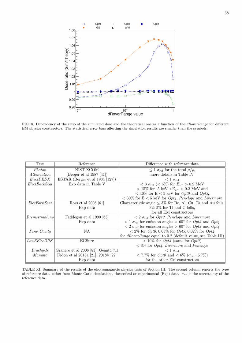
58

dRoverRange value

2−10 1−10 1

Do

se

ra

tio

(S

im/T

he

ory

)

0.98

0.99

1

1.01

1.02

1.03

1.04

1.05

1.06

1.07

1.08

Opt0 Opt3 Opt4

GS WVI

FIG. 8. Dependency of the ratio of the simulated dose and the theoretical one as a function of the dRoverRange for differentEM physics constructors. The statistical error bars affecting the simulation results are smaller than the symbols.

Test Reference Difference with reference data

Photon NIST XCOM ≤ 1 σref for the total µ/ρ,Attenuation (Berger et al 1987 [41]) more details in Table IVElectDEDX ESTAR (Berger et al 1984 [127]) < 1 σref

ElectBackScat Exp data in Table V < 3 σref (< 5%) for Ee− > 0.2 MeV< 15% for 5 keV <Ee− < 0.2 MeV and< 40% for E < 5 keV for Opt0 and Opt3,

< 30% for E < 5 keV for Opt4, Penelope and LivermoreElecForwScat Ross et al 2008 [61] Characteristic angle ≤ 3% for Be, Al, Cu, Ta and Au foils,

Exp data 3%-5% for Ti and C foils,for all EM constructors

Bremsstrahlung Faddegon et al 1990 [63] < 2 σref for Opt0, Penelope and LivermoreExp data < 1 σref for emission angles < 60 for Opt3 and Opt4

< 2 σref for emission angles > 60 for Opt3 and Opt4Fano Cavity NA < 2% for Opt0, 0.03% for Opt3, 0.02% for Opt4

for dRoverRange equal to 0.2 (default value, see Table III)LowEElecDPK EGSnrc < 10% for Opt3 (same for Opt0 )

< 3% for Opt4, Livermore and PenelopeBrachy-Ir Granero et al 2006 [83], Geant4 7.1 < 1 σrefMammo Fedon et al 2018a [21], 2018b [22] < 7.7% for Opt0 and < 6% (σref=5.7%)

Exp data for the other EM constructors

TABLE XI. Summary of the results of the electromagnetic physics tests of Section III. The second column reports the typeof reference data, either from Monte Carlo simulations, theoretical or experimental (Exp) data. σref is the uncertainty of thereference data.

59

0 0.2 0.4 0.6 0.8 1 1.20

0.2

0.4

0.6

0.8

1

1.2

1.4

1.6

1.8

2EGSnrc Livermore Penelope

Opt3 Opt4

1000 keV

0r/r

0 0.2 0.4 0.6 0.8 1 1.2

0.9

0.95

1

1.05

1.1

0 0.2 0.4 0.6 0.8 1 1.2

)0

)/d

(r/r

0d

(E/E

0

0.2

0.4

0.6

0.8

1

1.2

1.4

1.6

1.8


Opt3 Opt4

100 keV

0r/r

0 0.2 0.4 0.6 0.8 1 1.2

Mo

de

l/E

GS

nrc

0.9

0.95

1

1.05

1.1

0 0.2 0.4 0.6 0.8 1 1.2

)0

)/d

(r/r

0d

(E/E

0

0.2

0.4

0.6

0.8

1

1.2

1.4

1.6

1.8


Opt3 Opt4

10 keV

0r/r

0 0.2 0.4 0.6 0.8 1 1.2

Mo

de

l/E

GS

nrc

0.9

0.95

1

1.05

1.1

0 0.2 0.4 0.6 0.8 1 1.20

0.2

0.4

0.6

0.8

1

1.2

1.4

1.6

1.8


Opt3 Opt4

15 keV

0r/r

0 0.2 0.4 0.6 0.8 1 1.2

0.9

0.95

1

1.05

1.1

FIG. 9. Scaled DPK distributions for incident electrons of 10, 15, 100 and 1000 keV in liquid water, simulated using thefive Geant4 EM physics constructors. Ratios of Geant4 and EGSnrc results are reported as well. Dashed lines indicate anagreement of 3%, which corresponds to the statistical uncertainty affecting the Geant4 Monte Carlo simulation results.

60

Energy (keV)10 210

310

m)

µ (

ke

V/

Fy

1−10

1

10

SLDefault, cut100 eV SL1000 nm, cut100 eV SL100 nm, cut100 eV

SLDefault, cut1 keV SL1000 nm, cut1 keV SL100 nm, cut1 keV

FIG. 10. Frequency-mean lineal energy as a function of the incident electron energy, using two different values for the trackingcut 100 eV and 1 keV. SL is the step-size limit. SL was set equal to 1 mm (default value for this test), 1 µm and 100 nm.Error bars are not included since they are smaller than the symbols. The plot demonstrates that SL should be substantiallyless than the size of scoring volume.

0 2 4 6 8 10

Dose r

ate

dis

trib

ution

2−10

1−10

1

10 Ref Livermore Penelope

Opt0 Opt3 Opt4

Distance from source (cm)0 2 4 6 8 10

Sim

/Re

f

0.96

0.98

1

1.02

1.04

FIG. 11. Radial dose rate distribution with respect to r, distance from the center of the 192Ir brachytherapy source. The radialdose distribution is normalised at r=1 cm. Black squares in the top figure represent the reference data (from Granero et al2006 [83]), the statistical uncertainties of the data are within the symbols. The bottom plot shows the ratio of the Geant4simulation results and the reference data. The dashed lines indicate the statistical uncertainty affecting both the simulationresults obtained with Geant4 10.5 and the reference data published in Granero et al 2006 [83], obtained with Geant4 7.1.

61

FIG. 12. Left and center: Dosimeter placement and irradiation geometry modelled in the test. Drawings are not to scale.Right: Dose comparison between experimental data (black symbols) and the five Geant4 EM physics constructors for the depthof 3 cm. All the other depths are available in the geant-val interface. The black error bars represent the combined standardexperimental uncertainty (with a coverage factor, k=1), while the color ones are referred to the simulations data. The bottomplot shows the ratio between Geant4 and experimental data. The black dashed lines represent the 5% accuracy, a typicalthreshold accuracy considered in breast dosimetry.

Test Reference Difference with reference data

NucNucInelXS Zerkin et al 2018 [97] < 10% overallC12FragCC Toshito et al 2007 [24] < 1 σref for total and Li cross sections

18% for Be isotopes, 34% for B isotopes for QMD26% for Be isotopes, 36% for B isotopes for BIC38% for Be isotopes, 48% for B isotopes for INCL

TABLE XII. Summary of the results of the hadronic physics tests of Section IV. The second column reports the reference data,which are all experimental and published in the literature. σref is the uncertainty of the reference data.

62

310

Cro

ss

Se

ctio

n(m

b)

C6

12Proton +

performed with QGSP_BIC

2103

10Energy (MeV/u)

0.6

0.8

1

1.2

1.4

Ratio (

Exp/S

im)

O8

16Proton +


2103

10Energy (MeV/u)

310

Cro

ss

Se

ctio

n(m

b)

Al13

27Proton +


2103

10Energy (MeV/u)

0.6

0.8

1

1.2

1.4

Ratio (

Exp/S

im)

Ca20

40Proton +


2103

10Energy (MeV/u)

310

Cro

ss

Se

ctio

n(m

b)

C6

12Carbon +


2103

10Energy (MeV/u)

0.6

0.8

1

1.2

1.4

Ratio (

Exp/S

im)

Al13

27Carbon +


2103

10Energy (MeV/u)

FIG. 13. Total hadronic inelastic scattering cross sections as a function of the kinetic energy of the projectile, calculated bymeans of the QGSP BIC physics list. To note, differently from the other figures depicting the results of the tests of G4-Med,in the bottom plot ratios of reference data and Geant4 simulation results (and not the other way round) have been plotted forclarity reasons. Red curve: Geant4 cross section; data points: EXFOR reference experimental data.

63

3−10

2−10

1−10

1

10

210

310

He at 62 MeV/u4Cnat

C +12

°= 2.2θ

3−10

2−10

1−10

1

10

210

310 °= 7.6θ

0 20 40 60 80 100

3−10

2−10

1−10

1

10

210

310

Exp. Data

BIC

INCL

= 18θ

°= 4.9θ

°= 14.4θ

0 20 40 60 80 100

= 21.8θ

E [MeV/u]

[mb/s

r/(M

eV

/u)]

Ω∂

E/

∂/σ

2∂

He at 62 MeV/u4Cnat

C +12

FIG. 14. Double-differential cross sections measured at different angles of α-particle production in the 12C interaction with athin C target at 62 MeV/u as a function of the α-particle kinetic energy. Experimental data from De Napoli et al 2012 [103](in black) are compared with the two models available in Geant4 for ion interactions at this energy, namely INCL (in blue)and BIC (in red).

64

Fragment

Total Li Be B

Fra

gm

ent pro

duction c

ross s

ection (

mb)

210

310

Exp BIC

QMD INCL

Model/E

xp

0.40.50.60.70.80.9

11.11.2

FIG. 15. Comparison of Geant4 against experimental data for 12C total and partical charge-changing cross sections. The totalcharge-changing cross-section includes the production of B, Be, H, He, Li, N, O, α, deuteron, proton, neutron and triton. Theenergy of the incident 12C ion beam is 300 MeV/u.

0

20

40

60

80

100

0 0.5 1 1.5 2 2.5 3 3.5 4

Thick foil

Thin foil

Rela

tive d

ose (

A.U

.)

Depth (cm)

Livermore

Penelope

Opt3

Opt4

0.6

0.4

0.2

0

Liv.Pen.

Opt3

Opt4

Range

Geant4

measure

d (

mm

)

0

0.02

0.04

Spread

FIG. 16. Left: Depth-dose distributions in water for protons scattered with a Ta thin foil and a Ta thick foil calculated withfour EM physics constructors, while keeping the hadronic physics modelled by means of the QGSP BIC HP. Experimentaldata is shown with empty squares. Right: Differences between calculated to experimental parameters spread s (top) and rangeR0 (bottom) for the thin (empty markers) and thick (filled markers) foils. Errors and error bars represent 1σ and includeexperimental and Monte Carlo uncertainties.

65

Depth in water (mm)

0 50 100 150 200 250 300

(mm

)d

82

,exp

- R

d8

2,G

4R

4−

3.5−

3−

2.5−

2−

1.5−

1−

0.5−

0

0.5

1

Carbon

Livermore Penelope Opt0 Opt3 Opt4

Carbon

Depth in water (mm)

0 50 100 150 200 250 300

(mm

)d

82

,exp

- R

d8

2,G

4R

0.4−

0.3−

0.2−

0.1−

0

0.1

0.2

0.3

0.4

Proton

Livermore Penelope Opt0 Opt3 Opt4

Proton

FIG. 17. Absolute differences obtained between the depth at which the energy deposited was 82% of peak, at distal BraggPeak, calculated with Geant4 (Rd82,G4) and obtained experimentally (Rd82,exp), represented as function of the reported rangein water for each beam. Left: Results for proton beams at 125, 150, 175 and 200 MeV/u; right: Results for 12C beams at100, 200 and 400 MeV/u; here, Livermore, Penelope, Opt3 and Opt4 symbols exactly overlap. The estimated uncertainty ofRd82,G4, represented with error bars, was 50 µm in all cases (see main text for details); for 12C, symbols were larger than theerror bars.

Test Reference Physical Quantity Difference with reference data

LowEProtonBraggPeak Faddegon et al 2015 [25] 67.5 MeV proton Bragg PeakSpread < 1 σref (within 0.5 mm)Range < 2 σref (within 0.5 mm)

for all EM constructorsLightIonBraggPeak Schardt et al 2007 [114] 125–200 MeV/u protons, Rd82 < 0.1% (< 0.2 mm)

100–400 MeV/u 12C, Rd82 < 1.1% (< 0.8 mm) for allcases apart from Opt0

TABLE XIII. Summary of the results of the hadronic physics tests of Section V. The EM constructor is tested (Opt0, Opt3,Opt4, Livermore and Penelope) while keeping the same hadronic physics component (QGSP BIC HP). All the reference dataare experimental measurements. σref is the uncertainty of the reference data.

Test Reference Physical Quantity Difference with respect to reference data

ProtonC12 Meier et al 1989 [117] Neutron yield < 2 σref for QGSP BIC HP,NeutronYield Meier et al 1990 [118] of 113 MeV and 256 MeV p < 4 σref for QGSP BERT HP

ProtonC12 Satoh et al 2016 [119] Neutron yield < 11% against PHITSNeutronYield 290 MeV/u 12C < 50% against exp data

for both for QGSP BIC HPand QGSP BERT HP

FragTest Haettner et al 2013 [120] 400 MeV/u 12C QGSP BIC HP for hadronsfragmentation yield BIC and QMD : < 25% , INCL:< 40%

Hadrontherapy Petringa et al 2019 [27] Cell survival test QGSP BIC HP62 MeV proton beam < 20% for DU145

> 20% for MDA-MB-231

TABLE XIV. Summary of the results of the hadronic physics tests of Section V. The EM constructor is kept constant (Opt4 )while changing the hadronic physics component. All reference data are experimental. σref is the uncertainty of the referencedata.

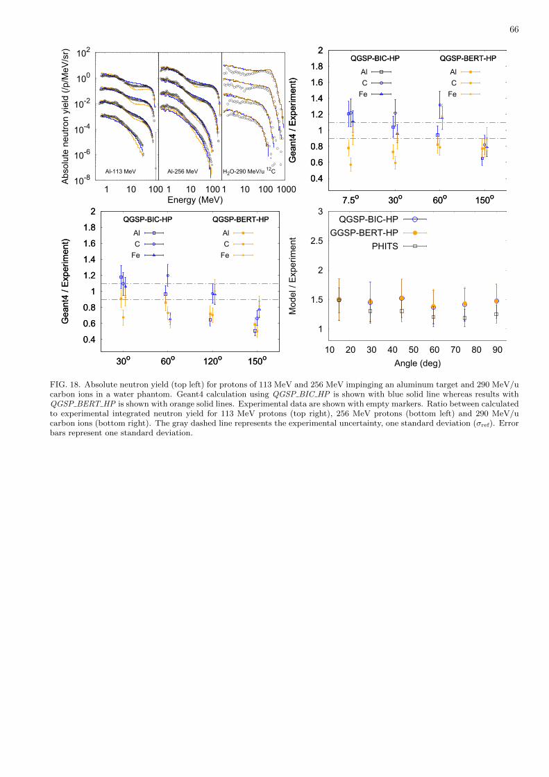
66

10-8

10-6

10-4

10-2

100

102

1 10 100

Al-113 MeV

Ab

so

lute

ne

utr

on

yie

ld (

/p/M

eV

/sr)

1 10 100

Al-256 MeV

Energy (MeV)1 10 100 1000

H2O-290 MeV/u12

C

0.4

0.6

0.8

1

1.2

1.4

1.6

1.8

2

7.5o

30o

60o

150o

QGSP-BIC-HP QGSP-BERT-HP

Ge

an

t4 /

Exp

erim

en

t)

Al

C

Fe

0.4

0.6

0.8

1

1.2

1.4

1.6

1.8

2

7.5o

30o

60o

150o


Ge

an

t4 /

Exp

erim

en

t)

Al

C

Fe

0.4

0.6

0.8

1

1.2

1.4

1.6

1.8

2

30o

60o

120o

150o


Ge

an

t4 /

Exp

erim

en

t)

Al

C

Fe

0.4

0.6

0.8

1

1.2

1.4

1.6

1.8

2

30o

60o

120o

150o


Ge

an

t4 /

Exp

erim

en

t)

Al

C

Fe

1

1.5

2

2.5

3

10 20 30 40 50 60 70 80 90

Mo

de

l /

Exp

erim

en

t

Angle (deg)

QGSP-BIC-HP

GGSP-BERT-HP

PHITS

FIG. 18. Absolute neutron yield (top left) for protons of 113 MeV and 256 MeV impinging an aluminum target and 290 MeV/ucarbon ions in a water phantom. Geant4 calculation using QGSP BIC HP is shown with blue solid line whereas results withQGSP BERT HP is shown with orange solid lines. Experimental data are shown with empty markers. Ratio between calculatedto experimental integrated neutron yield for 113 MeV protons (top right), 256 MeV protons (bottom left) and 290 MeV/ucarbon ions (bottom right). The gray dashed line represents the experimental uncertainty, one standard deviation (σref). Errorbars represent one standard deviation.

67

Exp BIC QMD INCL

50 100 150 200 250 300 3500

0.01

0.02

0.03

0.04

0.05

0.06

0.07

0.08 Z = 5

Thickness of Water (mm)

50 100 150 200 250 300 3500.2

0.4

0.6

0.8

1

1.2

1.4

1.6

1.8

50 100 150 200 250 300 350

0N

/N

0

0.1

0.2

0.3

0.4

0.5

0.6

0.7

0.8

0.9Z = 1


50 100 150 200 250 300 350

Ra

tio

(S

im/E

xp

)

0.2

0.4

0.6

0.8

1

1.2

1.4

1.6

1.8

50 100 150 200 250 300 3500

0.1

0.2

0.3

0.4

0.5

0.6

0.7Z = 2


50 100 150 200 250 300 3500.2

0.4

0.6

0.8

1

1.2

1.4

1.6

1.8

50 100 150 200 250 300 3500

0.01

0.02

0.03

0.04

0.05

0.06Z = 3


50 100 150 200 250 300 3500.2

0.4

0.6

0.8

1

1.2

1.4

1.6

1.8

50 100 150 200 250 300 350

0N

/N

0

0.005

0.01

0.015

0.02

0.025

0.03

0.035Z = 4


50 100 150 200 250 300 350

Ra

tio

(S

im/E

xp

)

0.2

0.4

0.6

0.8

1

1.2

1.4

1.6

1.8

FIG. 19. The fragment yields, N , produced from N0 mono-energetic 400 MeV/u 12C ions incident upon different thicknessesof water. The fragments were scored within a forward angle of 10 from the centre of the water targets. Experimentalmeasurements of fragments with different atomic number ranging from 1 to 5 are compared against alternative models availablein Geant4. The dashed lines on the bottom ratio plots indicate the experimental uncertainty σref.

-1Ω)

0(N

/N

2

4

6

8

10

12

14

16

18

Thickness = 288 mm, Z = 1

Angle (deg)

2− 0 2 4 6 8 10

Ra

tio

(S

im/E

xp

)

0.5

1

1.5

2

2.5

0

0.2

0.4

0.6

0.8

1

1.2

1.4

1.6

Thickness = 347 mm, Z = 4

Angle (deg)

1− 0 1 2 3 4

0.5

1

1.5

2

2.5

-1 )Ω

)(M

eV

0(N

/N

0

0.005

0.01

0.015

0.02

0.025

0.03

Thickness = 159 mm, Z = 2, Angle = 3deg

Fragment Energy (MeV)

500 1000 1500 2000

Ra

tio

(S

im/E

xp

)

0.5

1

1.5

2

2.5

Exp BIC QMD INCL

FIG. 20. Example angular and energy fragment distributions comparing experimental measurements against alternative modelsavailable in Geant4 for a 400 MeV/u mono-energetic 12C ion incident upon water. Left and Middle: Angular distribution ofH (left) and Be (middle) produced with a water thickness of 288 mm and 347 mm, respectively. Right: An example energydistribution of He fragments recorded at an angle of 3 from the centre of the 12C ion beam when incident upon 159 mm ofwater. The dashed lines on the bottom ratio plots indicate the experimental uncertainty σref.

68

0 0.5 1 1.5 2 2.5 3 3.5 4

Surv

ival F

raction

1−10

1

Experimental data

LEM III-weighted method

MDA-MB231

Dose [Gy]0 0.5 1 1.5 2 2.5 3 3.5 4

MC

/da

ta r

atio

0.20.40.60.8

11.21.41.61.8

22.2

0 0.5 1 1.5 2 2.5 3 3.5 4

Surv

ival F

raction

1−10

1

Experimental data

LEM III-weighted method

DU145

Dose [Gy]0 0.5 1 1.5 2 2.5 3 3.5 4

MC

/da

ta r

atio

0.20.40.60.8

11.21.41.61.8

FIG. 21. Experimental cell Surviving Fraction (SF) measured irradiating DU145 cells and MDA-MB231 (dotted points) and thecorresponding curves calculated with the LEM III-weighted method (triangles). Ratios of Geant4 simulations to experimentaldata are also plotted.

Report on G4-Med, a Geant4 benchmarking system for medical ...

Documents

Transcript of Report on G4-Med, a Geant4 benchmarking system for medical ...