REPORT NO. 1571

FORMULATION Of THE LARGE DEFLECTION SHELL EQUATIONS

ISE IN FINITE DIFFERENCE STRUCTURAL RESPONSE

COMPUTER CODES

Joseph l. Santiago CReproduc.d by

NATIONAL TECHNICALINFORMATION SERVICE

Spimfild, Va. 22151

February 1972

Approved lor iublc release; distribution unlimited.

U.S. ARMY ABERDEEN REv UEARCH AND DEVELOPMENT CENTER

BALLISTIC RESEARCH LABORATORIESABERDEEN PROVIN" GROUND, MARYLAND

wfu his report when it is no longer needed.: eturn it to the originator.

S.,condary ditrib1tIon of this report by o:riginati~g or

sponsoring activity is prohibited.

Addi•:ional copies of this report mey be purchased fromtic U.S. Department of Commerce, National Technicaltnfo,:.x.ation Service, Springfield, Virginia 22151

I.

=D

... ......... .............

The findings in this report are not to be con~strued asan official Department of the Army position, unlesssodersý.gnated by other authorized docu~ments.

4j

Unclassificd_____

DOCUMENT CONTROL DATA - R & D(S~W~f clssilcm n o t~le.bowof uobeftct sa"id adeu miants"He must be orsteed Whrn, ON* overall lopeif is dclasl id)

1. ORIGINATING ACTIVITY Wa~g ie Authat) IZ*. REPORT SECURITY CLASSIFICATIONU.S. Army Aberdee.. Research and Development Center UnclassifiedBallistic Research Laboratories GROUPAberdeen Proving Ground, MarylandF

. &O TITLE

FORMUILATION OF THE LARGE DEFLECTION SHELL EQUATIONS FOR USE IN FINITE DIFFERENCESTRUCTURAL RESPONSE COMPUTER CODES

4. oaeSCRivToVe NOTES (7VV o .srpas mad incluelvo *iss)

S. AU TMOSR(S) (Frst -.eve Aid. MftaI. zel etRame)

Joseph M. Santiago

so. REPORT OATE To. TOTAL NO0. OF PAGES or. "O. airEsFebruary 1972 158 18

80. CONITRACT ON GRANT NO. So. CRIGINATOWS REPORT NMUUERIS1

VftOJaCT %0. RDT&E 1T061102A14B and BRL Report No. 15721

1W062118ADSIa. Sb. OTH4ER REPORT NOfS) (AIW 0d nunbeg Stil fer 60 0901~m~

I0. OSTMIDUTIOW0 STATIAMIT

Approved for public 'release; distribution unlimited.

11. SUPIPLEMENTARY NOTES 1ia. 00ueSORINaS MILITARY ACTIVITY

U.S. Army Materiel Command

~. RCTWashington, D.C. '

A formulation of the equations governing the large transient deformation ofKirchhoff shells especially suitable for use in finite difference structural responsecodes is presented. It is shown how rfiese equations are employed in REPSIL, acomputer code developed at the BRL foE predicting the large deflection of thinelastoplastic shells subjected to blest and impulse loadings. The REPSIL formulationis compared with the somewhat similar formulations used by PETROS 1 and PETROS 2, twoclosely related ccdes developed by MIT.

S...pCES 00 Pm$a* I JA 0. SbSICK ofDD~ ,,..,*iqi'8I4LET Unclassified

vocrA ty clessidfices"

OnclassifielSectwity Classification

o4. LINK A L. K 8 LINK C

ROLl[ WT 11101-l9 WI ROLE WT

IKirchhoff ShellTransient ResponseFinite Difference MethodLarge Deflectiorn TheoryImpulsive LoadingPressure LoadingElastoplastic Material BehaviorStiain Hardening BehaviorStrain Rate Sensitive BehaviorComputer Program

A

UnclassifiedSe•wty C•ssiflcation

B BALLISTIC RESEARCH LABORATORIES

REPORT NO. 1S71

FEBRUARY 1972

FORMULATION OF THE LARGE DEFLECTION SHELL EQUATIONSFOR USE IN FINITE DIFFERENCE STRUCTURAL RESPONSE

COMPUTER CODES

Joseph N. Santiago

Applied Mathematics Division

Approved for public release; distribution unlimited.

RDT&E Project Nos. IT061102A14B and 1W062118ADS1

ABERDEEN PROVING GROUNDI MARY LAND

ii

SBALLISTIC RESEARCH LABORATORIES

REPORT NO. 1571

JMSantiago/j dkAberdeen Proving Ground, Md.February 1972

FORMULATION OF THE LARGE DEFLECTION SHELL EQUATIONS

FOR USE IN FINITE IIIFFERENCE STRUCTURAL RESPONSECOMPUTER CODES

ABSTRACT 7

A fo-rmlation of the equations governing the large transient defor-

nation of KirCIhoff shells especially suitable for use in finite differ-

ence structural respor:e codes is presented. It is shown how these

equations are. employed in REPSIL, a computer code developed at the BRL

for predicting the large deflection of thin elastoplastic shells subjected

to blast and impulse loadizgs. The REPSIL formulation is compared with

the somewhat similar formulations used by PETROS 1 and PETROS 2, two

closely related codes developed by NIT.

34

TABLE OF CONTENTS

Page

ABSTRACT............. ........... ......... ...... . 3

LIST OF FIGURES .-...... ......... ......... ........... ... 7

t LIST OF SYMBOLS ..... ......................... 9

1. INTRODUCTION ......... .......................... .... 13

1.1 Historic Background ....... .................... ... 13

1.2 Outline of Remainder of Repoxt . . . . .. . . .. . .. .. 1s

2. GEOMETRY OF A DEFORMING SHELL ..... ......... .. .......... 17

2.1 Motion of the Reference Surface .................. .... 17

2.2 Differential Geometry of the Reference Surface . . . . . 18

2.3 Kinematics of the Reference Surface ................ ... 23

2.4 Kirchhoff Hypothesis ...................... 25

3. STRAIN IN A SELL ........ .......................... 31

3.1 Definition of Strain ....... ................... .... 31

3.2 Strain-Displacement Relations ........ ............... 33

3.3 Surface Normal-Displacement Relations ............... 36

4. RESULTANT RELATIONS FOR MIDDLE SURFACE VARIABLES ............ 39

4.1 Integration Through the Shell Thicknes.. ............ 39

4.2 Linear Momentum and Spin Momentum Relations ..... ........ 43

4.3 Stress Resultant and Couple Resultant Relaticns ...... .... 44

4.4 External Force and External Couple Relations .... ....... 49

5. EQUATIONS OF MOTION OF A SHELL .......... .................. 53

5.1 Derivation oi" Equations of Motion ................. ... 53

5.2 Conservation of Mass ....... ... ................... S9

5.3 Reduced Equation or Motion ...... ................ .... 65

PR EEDING PAGE BIAMN1

i5

TABLE OF CONTENTS (Continued)I Page

6. BOUNDARY CONDITIONS FOR A SHELL .. .............. 71

6.1 Variation of Strain Energy ............... . 71

6.2 Classical Boundary Conditions along General Curves . . . . 77

6.3 Boundary Conditions along Coordinate Curves. ......... 82

6.4 Symmetry Boundary Conditions .... ............. . 85

7. MATHEMATICAL FORMULATION OF THE REPSIL CODE .......... 91

7.1 Equations of Thin Shell Theory ............. 91

7.2 Restricted Thin Shell Theory Used by REPSIL ........ .... 95

7.3 Description of the REPSIL Formulation .... ....... 99

8. COWPARISON OF ThE REPSIL, PETROS 2 AND PETROS 1 CODES ..... 107

8.1 Comparison of Theoretical Formulations ............ .. 107

8.2 Comparison of Major Computational Differcnces. .. ....... 117

REFERENCES. . . . . . . . . . . . . . ............. 123

APPENDICES

A- SURFACE INTEGRAL THEOREMS... ............ 125

SB- SYMMETRY BOUINDARY FORMULATION . . . . . ...... 129

C- ELASTOPLASTIC STRESS FORMULATION . . . . . . . .. 137

D - PHYSICAL COMPONENTS OF SURFACE STRAIN ......... 143

DISTRIBUTION L!ST .......................... . . . . . . 149

6

LIST OF ILLUSTRATIONS

SFigure Page

2.1 TV. d'-formation of a shell under the Kirchhtf,othesis, . . . . . 26

4.1 The volume V generated by varying c between the limits+ over the region S of the middle surface ...... 40

, 4.2 The surface S^ gj nerated by varying C between the limits

+ -ver the arc C. . . .41

-i. T action on the region S of the external force F,'.erna± c tuple c, stress resultant vector Q and

( v).ouple resultitt vector m ...N.. . " ..... 54

6.1 Deflection pattern .f the middle surface of a shell6-aforming symmetrically about a symmetry plane. . . . . 86

a I

t

p]

LIST OF SYMBOLS*

a determinant of a.,

a basis for reference surface

a dual of the basis a

a.,,a covariant and contravariant components of the metric (firstfundamental tensor) of the reference surface

b body force vector

b components of b in the basis gi

b b~ covariant and mi'•ed components of the second fundamentalba8bB tensor of the reference surface

c external couple per unit area of reference surface

* C tangential vector equivalent to c, c x n

Ca components of C in the basis aa 2 a

a a CaC* 7 C

^aaC normal vectors of magnitudes Ca, vis. Can

E Young's modulusC

E tangential components of strain tensor in the basis g

F external force per unit area of reference surface

SF* a F

FaF tangential and normal components of F in basis (a ,n)-ia

9 determinant of gij or equivalently g_,

g- •basis in Euclidean space

* g dual of the basis g.

Sg.,gKi covariant and contravariant components of the metric inEuclidean space

Superscripts and subscripts range over the integers as follows:latin 1.2,3; greek 1,2; script 0,1,2.

PRECEDING PAGE BLANK 9

4 I iA

LIST OF SYMBOLS (Continued)

h thickness of shell

spin momentum per unit area of reference surface

4v couple resultant vector per unit arc length, m ffV.

m couple resultant tensor

SN? bending resultant tensor, ma x n

Me bending components; Mc = M*a

Ssymmetric part of MCa

norp-R., vectors of magnitudes Ha, vis. M n

*as a~½ H'a

normal vectors of magnitudes M* , vis. M* n

n unit normal to reference surface

SN*a modified stress resultant tensor defined by (5.46)

P linear momentum per unit area of reference surface

Q stress resultant vector per unit arc length, Qa•v

Q astress resultant tensor~

QaC modified stress resultant tensor defined by (5.40)2

a a aQ shear components of Qa Qa = Q on

as a a aaQ membrane components of Q ; Qa = Qa^asQ modified membrane components defined by (5.35)

Q a Q

r position vector of particles on reference surface

I time

St ,t traction on bounding surfaces S and S of shell

t It : componIats of t and t in the basis gi1

10

LIST OF SYMBOLS (Continued)

Au displacement increment undergone by particles on the reference~ surface in the time interval At

v velocity of particles on the reference surface

• ,v tangential and normal components of v in basis (a ,n)

SV.v tangential divergence of v as defined by (2.27)

x position vector of shell particles, r + ýn

y Yresultant moments of mass density defined by (4.15)aaY a½ ky

r components of the connection of the reference surface, equalto the Christoffel symbols

66 Kronecker delta

as E ~cB oaran adcontravariant components of the se-ymti

tensor e of the reference surface

distance of particle from reference surface along n

u determinant of ia(

components of tensor relating g to a see (2.37)1

v Poisson's ratio

V --xterior unit normal to curve in reference surface, defined- in Appendix A

a• va ,v covariant and contravariant components of v

mate-ial coordinates of particle on reference surface

P mass density per unit volume

Sa stress tensor

uniaxial yield stress

a contravariant components of a in the basis g.

unit tangent to curve in reference surface, defined in- Appendix A

11 •

-. - -£~:~ -.- ~ - --~ - ~-

LIST OF SYMBOLS (Continued)

, SIT a covariant and contravariant components of T

Superscripts

(O8] antis)mnetric part with respect to the a and 8 indices, seefootnote p. 66

S(aB) symmetric part with respect to the a and 8 indices, seefootnote p. 66

values of variable at beginning and end of time interval At,cf. Chapter 3 and 7

one sided limits of variable along arc, used in Chapter 6

Subscripts

'a partial derivative with respect to a

la covariant derivative with respect to

- values of variable adjacent to symmetry boundary, employedin Chapter 6 and Appendix B only

12

I. INTRODUCTION

This report is mainly concerned with presenting a formulation of

the equations governin6 "c large transient deformaticns of shells, es-

pecially suitable ior use in finite difference computer codes. The

recent adaptation of these equations to REPSIL, a code developed at the

BRL for predicting the large deflections of thin shells subjected to

* - blast and impulse loadings, has resulted in a number of improvements,

which are also described in this report. While the equations as formu-

lated in the main body of the report are quite general, being restricted

only by t:-ie Kirchhoff hypothesis, as applied in REPSIL they are further

restricted to thin elastoplastic shells for which the rotatory inertia

is negligible. A detailed description of the REPSIL code will be in-

cluded in a forthcoming user's manual.

1.1 Historic Background

In order to put this report and the associated computer code REPSIL

in their proper relation to work done at the Aeroelastic and Structures

Research Laboratory of MIT on similar codes, a short history cf the de-

velopment of REPSIL is in order. .REPSIL has evolved from a computer

code developed by LEECH [1] originally called PETROS and now called

PETROS 1 since the recent development by MORINO, LEECH and WITMER [2] of

the improved PETROS 2. For its time PETROS 1 was the most sophisticated

code available treating the large transient respon.ae of shells. For this

reason it was one of the codes selected for use in the numerical analysis

portion of the research program on shells and structures at the BRL.

Upon close study, HUFFINGTON [3] found that PETROS 1 contained

a number of flaws, in addition to having a rather limited choice of

printing options. He discovered that the clamped edge boundary condition

SNuabers in brackets refer to the list of references on page 123.

13

• 2

was incorrectly formulated and that the linear approximation erployed in

the stress increment calculation duilng plastic flow gave stress states

outside the yield surface. He revised the code, by increasing the print-

ing options, adding plotting capability, correcting the clamped edge con-

dition and reformulating the stress calculation based on the exact quad-

ratic expression. The revised code was named REPSIL. The details of

the revised stress calculation are documented in [4]

In this early version, however, REPSIL still retained many of the

unsatisfactory features of PETROS 1. For example, only cylindrical

panels with clamped edges could be treated, the finite difference mesh

had to be square, the strain-displacement relation did not properly

account for the curvature ef the shell, the finite difference derivatives

along the boundaries were inconsistent, etc. Consequently, a complete

reformulation of REPSIL, including its theoretical foundation, was begun

at the BRL. The reformulation has advanced sufficiently to warrant

documentation of the present version of REPSIL. This report documents

the mathematical model on which REPSIL is presently based. A user's

manual documenting the computaticnal reformulation of REPSIL will followshortly.

The Aeroelastic and Structures Research Laboratory of MIT has also

undertaken a complete revision of PETROS 1, which has resulted in the

code PETROS 2 [2]. Although REPSIL and PETROS 2 share a number of

features, they are independent extentions of PETROS 1 and do not coincide.

The differences between REPSIL and PETROS 2, as well as their differences

from PETROS 1, are discussed in Chapter 8.

PETROS 2 [2] uses a slightly modified version of this stress calculation.

My colleague, Dr. Huffington, was responsible for first making meaware of some of these flaws.

14

CA

I

1.2 Outline of Remainder of Report

The next five chapters, Chapters 2 through 6, develop rigorously

the theory of the motion of shells subject to the Kirchhoff hypothesis.

Although a functional relation is presumed to exist between the stress

and strain components, none is explicitly used to develop the theory.

in keeping with the general nature of these chapters.

Chapter 7 is more directly concerned with REPSIL. First the general

theory developed previously is specialized to thin shells and the rota-

tory inertia is neglected. Moreover, the stress - strain relation for

any material composing the shell is assumed to be isotropic and linearly

elastic - perfectly plastic. These assumptions give us a convenient

version of the equations forming the mathematical basis of REPSIL, which

are then used to illustrate the computational algorithm employed by

REEPSIL to solve problems.

As mentioned earlier, Chapter 8 gives a comparison of REPSIL,

PETROS 1 and PETROS 2. First the theoretical and then the computational

differences are discussed. These are then summarized in tabular form.

The reader principally interested in Chapters 7 and 8 is advised

to read at the very minimum Chapter 2 in order to acquaint himself with

the differential geometric approach used in REPSIL, as well as in

PETROS 1 and PETROS 2, and if further time permits, he should skim

Chapters 3 through 5 to familiarize himself with the significance of

the more commonly encountered terms. Chapter 6 can be safely skipped.

Although the algorit.m is illustrated assuming perfectly plastic ma-terial behavior, actually REPSIL has the capability of treating strainhardening, strain rate sensitive materials through the use of themechanical sublayer model described in [2; Sect. 5.4.2].

1s

2. GEOMETRY OF A DEFORMING SHELL

In this chapter we present the mathematics needed to describe the

motion of a shell geometrically. This involves introducing cvnceptsand results from differential geometry. We first treat the motion of

the reference surface of the shell, after which the consequences of

assuming the Kirchhoff hypothesis for the deformation through the shell

thickness are obtained.

2.1 Motion of the Reference Surface

A shell can be &-scribed qualitatively as a three- imensioned bod"

having one of its dimensions. the thickness, small in comparison to its

other dimensions. Shell theory takes advantage of this property in

order to simplify the study of shells by reducing an essentially three-

dimensional theory to one defined on a two-dimensional subspace, i.e. a

surface. This is accLomplished by assuming that the deformation through

the thickness is of a known functional form. Once this is done, we need

only study the deformation of a given surface eibedded in the shell,

called the reference surface ,and the associated changes in the shell

variables defined on this surface.

Denoting the surface parameters by a**, the time by t and the

position vector in Euclidean 3-space relative to some fixed origin by

It is customomy to pick the reference surface to be the middle surfaceof the shell; that is, the surface equidistant from the bounding facesof the shell. However, whether a surface initially equidistant fromthe bounding faces remains a middle surface throughout the history ofthe deformation is a function of the form assumed for the deformationthrough tne thickness. Hence, when no form has been explicitly assumed,the term reference surface is to be preferred.

Index notation is employed throughout this report, with Greek indicesbeing tacitly assumed to range over the integers 1, 2. Hence,

PRECEDING PAGE BLAK 17

r , the motion of the reference surface is specified by the reference

surface deformation function:

aa

r = r (•a,t) , (2.1)

with E ranging over some connected region in the plane and t over

some interval of the real line. We demand that the mapping &e - r be

one-to-one for any time t. We also require that the function r (a ,t)

be sufficiently differentiable so as to guarantee the continuity of all

derivatives subsequently introduced. Moreover, we assume for simplicity

that the 40 are material coordinates; that is, for fixed a the image ra

of the point a under the mapping (2.1) represents the successive po-

si -ions of the same material point or particle on the reference surface.

2.2 Differential Geometry of the Reference Surface

In this section we are concerned with the spatial characterization

of the reference surface at some fixed instant of time. We will need

tc use the language of the differential geometry of surfaces in Euclidean

3-space. Our treatment of this subject is not meant to be exhaustive.

Rather, we aim to present only selected results with a minimum of proof.

In this section we shall not bot-er to indicate the dependence of vari-

ables on t explicitly.

By holding the parameter I constant and allowing ý2 to vary, we

generate a member of the family of ý1 = const. coordinate curves.

Conversely, by holding ý2 constant and varying 91 we generate a member

of the family of g2 = const. coordinate cuzaws. We require that these

two families of curves be independent in the sense that no member of

one be anywhere tangent to any menber of the other. Thus, these two

families define a curvilinear coordinate system on the reference surface.

Extended treatments of the differential geometry of surfaces can befound in numerous text books on tensor analysis and differentialgeometry, of which the following are a representative collection:EISENHART [6], SOKOLNIKOFF [7] and ITOMAS [8].

18

-4-•

I

The partial derivative of the function r (Ca) with respect to

holding &2 constant

a (ca) =r 1�,at (2.2)

defines a vector tangent to a 2= const coordinate curve and the other

partial derivative holding ýI constant

!2 C r '2 (,a) (2.3)

a vector tangent to a = const coordinate curve. We require that

the vectors a nowhere vanish. Hence, by virtue of the previously

assumed independence of the families of coordinate curves. the pair a

form a linearly independent set of vectors tangent to the reference

surface and hence serve as a basis for vectors tangent to the reference

surface. They are in fact the basis generated by the coordinate curves.

The unit normal to the surface is simply

a xan C•) - (2.4)

Clearly the triad (aa, n) forms a basis for vectors in 3-space, with

the special orthogonality property that

n a a= 0 (2.5)

We use the comma notation for partial derivatives with respect tomaterial coordinates: a partial derivative with respect to &a isdenoted by a subscripted comma followed by the index a ; that is,

"19

The covariant components of the metric or the first fundawental

terxsor of the reference surface are defined as

a = a , a . (2.6)

They form a symnetric and positive matrix. Denoting the determinant of

the metric matrix by a, we have

2 2a - Det a 6 = a1l22 - (a 1 2 ) = 1aI x a2 > 0 (2.7)

The contravaiant co•rqonents of the surface metric can then be defined

as

11 12 21 22a .a 2 2 /a, a a 1 2 /aa , a =a 1 1 /a, (2.8)

and they also form a symmetric and positive matrix. Moreover, a is

the inverse of a8 :

a ay' aaY aY=6* a (2.9)ay ay ya a

with 6 8 {= 1 when a= = ,= 0 when ot j B) the Kronecker delta. By em-

ploying the contravariant components of the metric tensor, the duan

basis is generated:

a a aBa . (2.10)

The dual is inversely related to the basis a and is also normal to the-CE

We employ the summation convention: terms having a repeated index, onceas a subscript and once as a superscript, are to be summed over therange of that index.

20

surface normal n:

a a0 a n=0. (2.11)

*P- co-variant and contravariant components of the skew -syffrnnetric

qurface tensor e are defined as

a•2 as - aCB =a ea , = a½ e , (2.12)

where e (= 1 when a 1 =0 2,= - when = 2 & S 1,

= 0 when a = 6) is the permutation symbol. The components of c and the

Kronecker delta satisfy the Lsual relations:

C CY 6 =6 6 6 , £CyL Y C = 2 (2.13)y 6 6 y 6 " y6

Using the c tensor, we can summarize the -relationships between the basis-aa , the dual basis a and the surface normal n in the following compact

-ai

forms:× as= •n a B iBn

a xa c , a x a c n , (2.14)_a.c -8 as-.-

"••^B i ciBa

n x a cxa = .a

A tensor as important as the metric or first f-mdamental tensor for

surfaces embedded in 3-space is the second fund=ental tensor, which

measures the. spatial rate of change of the normal n with respect to the

surface basis. Its covariant components are defined as

b =-a • n a n , (2.15)

i is only a tensor under coordinate transformations with positive* Jacobians since the permutation symbol ear transforms like a relative

tensor of weight ±1; cf. SOKOLNIKOFF [7; p. 1071.

' ' i

the last equality clearly showing that the b tensor is symmetric. Simi-

larly, the components of the connection for the surface are defined as

r aY = ay = ay " r (2.16)

with the symmetry with respect to the first and second indices exhibited

by the last equality. A standard reduction relates the components of

the connection to the partials of the metric components

ra ='a (a B6,a + a 6a,8 aa, . (2.17)

Hence, the components of the connection are the Christoffel symbols.

It easily follows from this that

a 2 a½ k aYa =a . (2.18)2,a =2 S,a tas

The covariant derivative of any quantity with respect to a, denoted by

an attached subscript l a, is defined in the usual way through the

connection. The surface metric and the surface tensor e have the

prnperty that the covariant derivative of their components identically

vmaish:

a 0 ,a = , 8 1a , £ 0=a 0. (2.19)

See SOKOLNIKOFF [7; p. 129].

** 8BFor example, the covariant derivative of the two index quantitywith respect to &a is Y

_B Y a + rr y

cf. EISENHART [6; p. 110] or THOMAS [8; p.54].

22

- - - - ~ - ' ~ -

I This well kn-.,n property shall be fret-ly used throughout. It easily

follows from this property and the definition of the second fundamental

*.ensor that

a a aSa a n . a =b n n 1 b a a (2.20)

Note that the components of the metric are used to raise and lower the

indices of the second fundamental tensor (i.e. b' = aaby), as is

commonly done with the components of any tensor associated with the

surface. Lastly, we make mention of the fact that due to the second

fndamental tensor and the connection being defined as derivatives of

the basis a they satisfy the Codazzi and Gauss equations

b - b = 0 R = bb b bb 6 (2.21)

where

V V P V ) 1R =a (r -6 r 68 + ry r y1 r 60r -Yj (2.22)

is the Riemzan Christoffel curvature tensor for the surface.

2.3 Kinematics of the Reference Surface

The time derivative holding the material coordinates constant is

the material derivative. The material derivative of the function

r (Ea,t) is the veZoeity at the time t of the particle with materiala.

coordinates :

v(,a,t) =r(,a,t) .(2.23)

Resolved into normal and tangential components, the velocity becomes

v =v a + v n (2.24)

*a

Cf. EISENHART [6; p. 2191 or THOMAS [8; p. 89].

A superposed dot denotes the material derivative.

23

2NThe covariant derivative of the velocity, ;he meocity gradient, is also

resolved into normal and tangential components

F V (v b v) a8 + (va + b v ) n , (2.25)

using relations (2.20). A reversal of order of differentiation shows

that the velocity gradient is the material derivative of the basis:

v =~1a _a (2.26)

The divergence of the velocity v can be written as

V-v aL •*v = v - by v (2.27)l i la a (

Combining the last two equations, we obtain the useful relation

a2 1 k½ % aa8" a½ V-v (2.28)

Since the normal vector n is of constant munit) magnitude, its

material derivative w will be tangential to the surface and hence have

the resolution:

a aAlso, since n and a! are normal, their material derivatives cannot be

totally independent, but must. indeed, satisfy the relation

w *a +n v =0 ( (2.30)

from which it follows that

w=- n v a (2.31)

or, using (2.25) and (2.29),

a =-v la + basv) (2.32) ;-

242 -G

• !_-I

The latter allows us to write the velocity gradient in the form

v~ =(v b v) a~ w n .(2.33)

Interesting results could now be obtained relating the material deriva-

tives of the metric, second fundamental tensor, connection, etc. to vari-

ous covariant derivatives of the velocity components, but since the ma-

terial presented suffices for subsequent sections, we will Pot pursue

this line.

2.4 Kirchhoff Hy•pothesis

The Kirchhoff hypothesis assumes that the shell deforms in such a* way that particles initially on a normal to the reference surface will

find themselves after the shell is deformed on the same normal with their

distance from the reference surface unchanged. This hypothesis is an

idealization of tne observation that in many situations very little

shearing or extension ozcurs through the thickness over major portions

of the shell during deformation.

We shall assume that the shell is of uniform thickness and identify

the reference surface with the middle surface of the shell, although any

surface parallel to the middle surface would give an equivalent theory.

Using the coordinate system introduced previously, we have by the

Kirchhoff hypothesis that a particle located a distance ý from the

middle surface along the normal n passing through the middle surface

paicicle with coordinates • , will always be situated on the normal

through the same middle surface particle at the same distance ý. Hence

for all time the position of a particle is specified by the equation.

x = r i( ,t) + • n (ýE,t) (2.34)

* as indicated in Figure 2.1.

Notice that a particle off the middle surface will always have

associated with it the same coordinates ( w ,1), with < ý 0. Moreover,

a particle on the middle surface is always associated with the coordinates

25

C2.:; -- - -4-) ~

0 ZI4.LCC)

00- CL

E4-o r

(4- 0 0

0)

*g- G )

43

~03r. - C

XI03

- -

4- -O U

0 3*

0n 03

4.. 44-3

oý 4-3 4.)

5.4 .) EU

=S EUE0 0 S-

0 U- L..4-4- E

26

eJ

(• ,0). Hence the triplex , defines a material coordinate system

for all the particles composin- the shell. Taking h to be th uniformthickness dimension of the shell, r will range between the limits h

a 2while as before a range over some suitable connected region in the plane.

Definitions (2.23) and (2.29) allow us to write the particle velocity

asv + W (2.35)

The derivatives of (2.34) with respect to material coordinates (a, )define a basis in 3-space:

XC8, g3 - . (2.36)9 . 8 93 ,

From (2.20)3 it foilows that the basis g. is related to the basis

(a ,n) through the relations

8 g 3 n (2.37)

where the convenient abbreviation

6 y by (2.38)8= 8 - 8 b

is employed. The pair g8 (8 ,) defines a basis for the lamella

parallel to the middle surface at a distance • . When g = 0 the basis

reduces to the middle surface basis a . Notice that n is normalto each lamella, since

n g =0 (2.39'

Latin indices are introduced for the range 1, 2, 3.

27

, -

A metric for that portion of space occupied by the shell can be

specified using the basis g. as follows

gij ` gi "j (2.40)

The -leterminant and inverse of the metric are then defined in the usual

way

I ijk lmnDet gij e e gil gjm gkn

i 1 i ike " (2.41)g - e eJ gm g2g gkm ln'

wher e ijk (= 1 when i, j, k is an even permutation of 1, 2, 3; = -1

when i, j, k is an odd permutation; = 0 when i, j, k not distinct) is

the 3-dimensional permutation symbol. The inverse allows us tc define

the dual basis

g 1 g gi , (2.42)

having the reciprocal property

i ijSg -*gj = . (2.43)

The metric and its inverse assume the simple forms

911 g12 0\gij 921 g22 0 gij = 21 g22 (2.44)

due to g3 being a unit vector normal to ga . Hence we need only work

with the metric g of lamellar parallel to the middle surface and its

inverse g .Moreover the determinant g and dual basis g" become

28

g =Detg =g, e2 gay g6

(2.45)a ao 3 g ng=g g 8g g= g 3 n

Using (2.37), we relate the above quantities to the corresponding

middle surface quantitiesL

ga 6 aS -la=-l a6

(2.46)

a -la 8(U)2 g =11 a

al a

where and P denote the determinant and inverse of v:

11 1 e e e U'6 U e elay (2.47)

Clearly, the basis g , its dual g , the metric g and its

inverse only exist when v # 0 . It can be shown* that a sufficienthcondition to guarantee existence for r in the range ± is h < 2 Rmin

where R i is the minimum principle radius of curvature of the middle

surface. With this condition p > 0 We shall assume this mild con-dition to hold in developing the theory of general Kirchhoff shells, in

Chapters 2 through 6. In specializing the general theory to that forming

the basis for REPSIL in Chapter 7, we go further and require that the

more stringent thin shell hypothesis holds, wherein h << R so thatterm of ore2 mrin'terms of order k b8 b can be neglected in comparison with unity.

See NAGHDI (9; p 17].

29

I ________A

3. STRAIN IN A SHELL

In this chapter a measure of strain is defined based on the change

in the metric. This measure is simplified using the Kirchhoff hypothesis.

Equations are next obtained relating the incremental change in strain

to the gradients of the displacement increments of the middle surface.

3.1 Definition of Strain

Strain is any quaintity measuring the amount of stretching that

occurs in the local neightorhood of a particle during deformazion. The

differential vector coimecting the position r (tlc) of a particle with

the position r (ta + dta, C + d4) of any neighboring particle is given

by

dr = g dtc + g d . (3.1)-a -3

The distance ds between these particles is the magnitude of dr , or

dS2 =g dta dt + (g 3 +ga) d d + g dC2 " (3.2)

Initially at time t = to this distance is given as

&0

dS2 = G da d6 + (G 3 + G) dEa d + G d 2 * (3.3)aB l 33

A measure of the stretching undergone from the time t = t is0

Throughout this report the initial values of variables when t = twill be denoted by replacing minuscule by corresponding majuscule°letters, whenever this can be done without ambiguity. Otherwise azero subscript will be appended to indicate initial values.

PREC DING PAGE KIA K I--- ---- -- |~~ ~~--

(ds2 dS2) =E dadW + (E +E d~a d; +E dz 2 (3.4)aB OL 32 33

where

E. (g.~ G.. (3.S)11Eij 2 (ij - ij)(.5

This measure vanishes when no stretching occurs between two particles.

Moreover when no stretching occurs in the neighborhood of a particle,

so that the measure of stretching vanishes for all dia, d; , then E..13will vanish. This makes it reasonable to adopt E.. as a strain measure.13

Due to the Kirchhoff hypothesis, ga 3 = g 3 a = 0 and g3 3 = 1 for

all time. Consequently, the strain E.. will assume the simple form1)

(E1 1 E 1 2 0\

E.i= E2 1 E 2 2 0 (3.6)

0 0 0

This shows that no stretching or shearing takes place in the transverse

direction. Hence we need only consider the nonzero components of the

strain, namelyFIEc =2 (ga - G•S (3.7)

Clearly, the symmetry of g a implies the symmetry of E .

By virtue of (2.7,8) and (2.46)1 the nonzero components of strain

can be related to the surface metric and b tensor:

E [(a - A 0) - 2 (b - BaS) +2 (b2 B2 ) , (3.8)

where b 2 dentotes the components of the square of the second funda-

mental tensor:b2 b b 6

. (3.9)

32

From the definition of b (2.15) and the fact that n is a unit vector,r0

it follows that b2 can be written as

Sb 2 =n n, =- n n, (3.10)ac .-'a c

Clearly b 2 Is symmetric.

3.2 Strain - Disp'acement Relations

Let Au be the displacement undergone by a middle surface particle

from sone past time t- to the current time t. Denote the values of

variables at the time t- by an attached minus superscript and leave un-

changed the values corresponding to t. Using this notation, the dis-

placement Au becomes

Au -r - (3.11)

The strains at these times are

E = [(a -A )-2 (b B + ý2 (b 2 - B 2

as 2 as uta ais a$ as~ cx

(3.12)

E (a - A ) - 2i (b - B ) 2 W - B2 )A

Hence, it follows that the finite strain increment is additive:

E =E +AE , (3.13)

where the incremental strain is given by

AEa8 = •- [Aaaa - 2A bbs . (3.14)

and

Aa =a 8 -a, Ab =b -b Ab 2 =b 2 -b 2 (3.15)'Es as aB as ciB cis "

33

In order to express the strain increment in terms of gradients of

Au and An , we first observe that

Au a -a , An =n n - (3.16)

V Hence, from the definitions of a 8 b and b2 equations (2.6)a c e t (.

(2.15) and (3.10), we have

Aa,= a -*Au, +a Lu + Au Au,

Ab =n - Au,CO + An a a0 + An Au, (3.17)

Abl, 2 = n n + An +:. •An a n',

MB -_ .,- ,L -,a

or combining differently, we also have

Aa =a Au +a *Au - Au Au

a -a -,Bs -8 -,a _,a - ,

Ab = n Au. + An * a - An. Au (3.18)- ~,as -a.c,$ as ,z

Ab2 = n A + n An An -Aot -. ._,a A ,a

With these two sets of expressions we can write the strain increment

in the following equivalent ways:

AE -(a- -Au +a, *Au + Au -*Au )az 2 -.a ..,B _,a -, ,a ,

-24 (n- Au,+ An a + An Au ) (3.19)- • a+ -L , a ,CIO

+2 (n-. An +, n An + n , An)

34

II

AE "- (a Au +a Au u A-u

-2 (n Au + An a -An Au ) (3.20)

+ý2 (n an + n *AD &n

Both these expressions are exact within the limits of the Kirchhoff

hypothesis. They are quadratic in increments, with no linearization

based on the smallness of these increments being used. An exact ex-

pression linear in the increments can be obtained by averaging these

expressions:

AE ="[(a -Au +a Au,)

ax 2 -a ., . ,

-2 (n Au + An ) (3.21)- asi -a aa

+2 (6, .An + n An,)]

with- 1 - - 1== (a + a) n (n + n-) (3.22)

It should be noted that the last quantities have no significance other

than as averages, there not necessarily being any intermediate position

of the middle surface for which a forms a basis and n a surface normal.Indeed, .n will not generally be a unit vector nor be normal to a.

35

S

E

E

3.3 Surface Normal - Displacement Relations

When the gradient of the displacement increment Au is small, there

is; very little difference between n and n. This makes the use of (3.16)2

unsatisfactory for determining An numerically, since computational ac-

curacy could be impaired, and suggests the use of a linear expression

based on expanding An as a series in Au . On the other hand, for

moderately large Au the liniear expression would lose accuracy. Since

our aim is to ultimately use this theory in a computer code, these con-

siderations lead us to derive an exact expression for An containing

Au as a linear factor.

We begin by noting that due to n being a unit vector

An (n + n) n-n) (n +n)= , (3.23)

and due to n being normal to a

An * a = - n * a = - n Au (3.24)_a _~- a -a

Resolving An relative to the basis (a, n), we obtain

An =An aa +L n (3.25)

The tangential component,

An =An * a (3.26)

can be written as a linear expression in Au by using (3.24)

An =-n *Au (3.27)

As far as the author is aware, MORINO, LEECH and WIThER [2] are thefirst to have addressed themselves to this problem. The presentanalysis is partially based on theirs.

36

In order to cbtain an appropriate expression for the normal componet of

An, we multiply (3.25) by (n + n-). By virtue of (3.23), the product

vanishes so that

An n • a + + n n )An= 0 (3.28)a.

Solving this equation for An and using (3.24) and (3.26), we obtain an

expression quadratic in An and hence quadratic in Aua8

a An Ani "8

P An = - (3.29)l1 n " n

To insure that the denominator does not get too small and thus reduce

conutlational accuracy, we require that the above expression for An be used

only when the mild restriction n - n > 0 is satisfied, otherwise (3.16)2

should be used.

Rearranging slightly, we can summarize as follows: when n * n > 0,

determine the increment An using

AnAn= [a + n] An , (3.30)

~+ " " l n -n-

with

a asAna = n- •Au, " an a an6 (3.31)

otherwise when n * n < 0, use (3.16)2. Lastly, had the basis (a , n )- - -.a -

been used to resoive An , the expression for An would have assumed the

similar form:

AntAn = + a n-] Ana , (3.32)" .a l+n n

where now -a0An =-n Au , An =a An8 (3.33)

a a

37| IP

M-P 61&1

4. RESULTANT RELATIONS FOR MIDDLE SURFACE VARIABLES

Under the assumption that the shell deforms according to the

Kirchhoff hypothesis, we derive in this chapter relations connecting the

t I variables defined on the middle surface to associated variables defined

on the shell. More specifically, we obtain the relations connecting

1° the linear momentum and spin momentum densities acting on the middle

surface to the particle velocity field, f the stress and couple result-

ants to the stress field, and .' the body force and body couple resultants

to the body force field and tractions on the bounding surfaces. For the

derivation we also assume that the material composing the shell is non-*

polar and that the middle surface variables are resultants of the corre-

sponding quantities defined on the shell.

4.1 Integration Through the Shell Thickness

In order to obtain the resultant on the middle surface of a variable

defined on the shell, we need to express the volume integral as an inte-

gral over the middle surface of an integral through the thickness. We

begin by letting S be any region in the middle surface bounded by the

simple closed curve C. Let V be the portion of the shell geuerated by

varying ý between the limits t--as ranges over S, see Figure 4.1.The volume V is bounded by two surfaces h (where , and S

h+2(where t -_), and by the surface Sc generated by the bounding curve C as r

ranges between its limits. Using the basis gi , we can write the volume

integral of any variable 6( ) defined on V as

J C~al.) dv = 2LI ( hai) d dQ1 dt2 (4.1)

SV • h

See NOLL & TRUESDELL [10; Sec 98).

4See SOKOLNIKOFF (7; Eq 44.11].

PRECEDING PAGE BLANK 39

JAI

Se

Ti

Figure 4.1 The volume V generated by varying c between the limitsy over the region S of the middle surface. S is bounded by the

curve C and V by the surfaces S., S, and S_.

wherein Q is the pre-image of S (see Appendix A). By virtue of (2.46)3

the last expression becomes

JJ6(El ) dv P [dg] i a~ dtl dý2 (4.2)V h2

or, since S is the image of .I

h-

2dv u d' [f (4.3)

which is the desired integral representation. A similar argument yields

the representation

40

Li-- 5

°n

Figure 4.2 The surface S generated by varying between the limits_+ hover the arc C. T is the unit tangent to C and v the exterior unit

normal to C tangent to the middle surface. v* is normal to S4 and T*

is tangent to SA and the middle surface, but v* and -r* need not beunit vectors.

(E') da = JJ ( d.) + da (4.4)

S,. S

for any function 6 (a) defined either So S , with v and _ theh hrS •values of u at =-and r, respetivel.

We now seek an expression relating an integral over the bounding

surface S to an integral along the curve C of an integral through theL thickness. We begin by taking some connected subset of C, say the arc

C, and the surface S. generated from C by varying h r - as shownin Figure 4.2. Let 6 (s, ý) be a function defined on S. with s the

arc length along C. The integral A (s, ) over S. can be expressed asc

This expression is exact only when h = const. However, for slowlyvarying h it is a good approximation.I 41

+ h

(s,) da [J26 (sC) I v* I dc ds*, (4.5)

Ca 2

where v* is the (not necessarily unit) outward normal to Sa given by the

expression

it = V T x n , (4.6)

with

r - g T- (4.7)

by virtue of (2.36). It should be carefully noted that -r denotes the

components of the unit tangent -r to C with respect to the basis a .O

can be shown, using (2.14) 3 , (2.46)4 and (2.47)2 that

g xn=- u c ga (4,8)

which when used in conjunction with (4.7) enables us to write v* as

V* = 1 C T ag (4.9)

or, in view of (A.9) 2 , as

V* = 81 V (4.10)

The reader should notice that v8 represents the couponents with respect

to a of the unit outward normal to Sa along C. The last expres ion

could be substituted in (4.5), but we refrain from this since no simpli-

fication results at the moment.

See SOKOLNIKOFF [7; p. 151].

42

i%

4.2 Linear Momentum and Spin Momentum Relations

For the following derivation we add to the Kirchhoff hypothesis the

two basic assumptions: 10 the momentum density of particles composing

the shell is the product of the mass density and particle velocity and

20 the linear momentum and moment of momentum acting on any portion of

the shell are the resultants of the linear momentum and moment of mo-mentum densities of the particles composing that part of the shell.

We begin by endowing the middle surface with inertia by ascribing

to each point composing the surface a Zinear momentwn P per unit area

and a spin moment-m Z per unit area. Using the notation of the last

section, we have as a consequence of applying the above assumptions to

the volume V the two integral equations

P da =ff x v .ff (r xP + Z) da xx (Px) dv (4.11)

S V S V

with p the mass per unit volume and x the particle velocity. Upon

applying the integral representation (4.3), these become

g ~h -

JP da=Jf! P vd da~f Jh 0• d d

ST(4.12)

h

( rxP +)da J x x u d[ da

Since S is arbitrary, it follows from the continuity of p and x that theintegrands are equal:

h h

P 2 Px P d r P 2h P x x udc (4.13)

43

!3

By virtue of the Kirchhoff hypothesis,(2.34) and (2.35), the last equa-

t i ons become the momentwon-velocity relations

P= Yo V + Y1 W , W n x (YI v + Y2 w) , (4.14)

where Yo, Yl, y2 are the zeroth,first and second resultant moments of

mass density, defined by the general expression

h

Y= h 2 p (,)a dý (a = 0, 1, 2) (4.15)h_2

Tihese resultants have physical interpretations: yo is the mass per unit

middle surface area, yi is the product of the mass per unit middle

surface area and the distance from the middle surface to the center of

mass, and Y2 is the moment of inertia of the section relative to the

middle surface. If the center of mass were to coincide with the middle

surface, then y1 would vanish and Y2 would be minimum.

4.3 Stress Resultant and Couple Resultant Relations

Since we assume the material to be nonpolar, no couple stress field

is defined over the shell and only a (force) stress field need be con-

sidered. The force and torque act.-ng on any finite surface element are

assumed to be the resultants of the stress and the moment of stress

acting on the surface element.

Let C be any closed curve in the middle surface, then we assume

that the action of the surface exterior to C on the part interior to C

is equivalent to a stress resultant vector QOv" per unit arc length*

and a coua resultant vector rm() per uiit arc length. It is to be

This is a statement of the stress principle for shells postulated byERICKSEN & TRUESDELL [11].

44

expected that these resultant vectors will be functions not only of the

point through which C passes but also of the curve C itself. We anticipate

that the dependence on C will be through the exterior unit normal v iL

the curve tangential to the surface by writing the stress resultant and

couple resultant vectors with subscript (v).

Using the notation introduced in 4.1 and applying the above assump-

tions to the surface S- generated by the arc C subset of the closed curveC

C (see Figures 4.1 and 4.2), we obtain

SQ.,,ds = ao • da

C S-.C (4.16)

(r xQ +m ds x a vda

•:C S^C

with a the stress tensor and v the unit exterior normal to S, so that

a • v is the force per unit area over Sa . Since v is a unit vector co-

linear with v*, we can write

-. Iv*I V^ (4.17)

so that on applying the representation (4.5) to the above integrals they

become

h

-- ) 2 [ a v* d ds

- (4.18)

S• h

J (r x Qc() +1ml)) ds [ hx a - v* d ds

C C

F 45

Since these integrals hold for all arcs C subsets of C, it follows from

the continuity of the stress tensor that the integrands are equal, so

that in view of (2.34) we obtain

h h

Q = * d , m = n x a v* , d4 . (4.19)(Vo) h ~V ] h -

Next we use (4.10) enabling us to write Q( and m Q) as linear functions

of the componeats of the exterior unit normal v to the arc C:

h

?(V) = h - l a

2 (4.20)

h

m = x 2 . ga P 4 d] v

-(V h *

2

Or defining the stress resultamt tensor Qa and coWle resultant tensor*

m as follows '4

h haq 2a ga a 2ha- a

Q = d , m =n x a g p4d• , (4.21)- h h

22

(notice that both are independent of the curve normal v), we can finally

Qand m are called tensors because each is pair of vectors in 3-spaceThat, in addition, behave like couponents of vectors in the (2-dimen-sional) tangent space of the middle surface under transformation of thematerial coordinates Ca. More properly they should be called doubletensor fields, see [11; Eq. 3.1] for a definition.

46

t21

I • -• -'- •i- • • ... •' • -•-w• - • .. . •.-•-• - • - ° "•• ... . ...

I

write the stress and couple resultant vectors as

Q Qvm = mv . (4.22)

Because ma lacks a normal component, as is clear from (4.21)2, we

find it convenient to introduce an equivalent tensor Ma, the bending

resultant tensor, through the definition

a aM m n , (4.23)

with the equivalence of these two tensors following from the conjugate

relation

a Mam =n x M (4.24)

which is a consequence of (4.21)2. Like ma, le only has tangential

components.

aaThe stress resultant Q and bending resultant Ma are conveniently

resolved relative to the basis (a , n)

Qa Qa8 aB+Qa n Ma =M aQ Q Q nMa a(4.25)

and, by virtue of (4.21) and (4.23), we obtain for their components

These relations could also have been "'tained from integral equationsof equilibrium by arguments based on tne continuity of the integrandsand the arbitrariness of S, c f. ERICKSEN & TRUESDELL [11; Sect. 24].

47

h h=a a g V dý Q n a g a dr.,

" h " ~- h "

(4.26)

h= • * d

Sh2

Writing the components of the stress a relative to the basis g. as

follows

a =g gi (4.27)

we can, using (2.45)3 and (2.46)4' replace a by its components to obtain

h hasQ2 2 3adQ Usf Ba"v d:, Q' ah jidJh Y• = Ih •

2 2 (4.28)

hM ya r dý

By convention we call QaB the nmPbra-ze co-onent and Qa the shear

conponents of the stress resultant. The last relations, as well as the

one before, will hold irrespective of how the stress is obtained from

the strain and/or strain rates, etc. AltInugh not used in this deriva-

tion, the stress is assumed to be symmetric

ii 3ia a , (4.29)

in line with the nonpolar nature of the material.

48

4.4 External Force and External Couple Relations

Again, using the fact that the material is nonpolar we consider

only a body force field defined over the shell. We assume that the

force on a finite volume is the resultant of the stress acting over the

volume's botundary and the body force acting over the volume, and that

the torque on the volume is the resultant of the moment of stress over

the bouidary and the moment of body force over the volume.

We begin by accounting for the influence of the external environ-

ment on the middle surface by assigning to each point on the surface an

external force F per unit area and an external couple c per unit area.

We then apply the above assumptions to the volume V bounded by the

surfaces S., S+ and S_ (see Figure 4.1) to obtain, after taking care to

eliminate the contributions from S by applying (4.16) to C, the two

integral equations

JFda =J b dv + t da + t da

S V S S (4.30)

IfJ (r xF c) da fjffxx bdv +Jifx x t da +Jfx- xt da,

S V S. S-

with b the body force, and t+ and t_ the tractions on the surfaces whereSh h -+

= 5-and , - - , respectively. Since the exterior unit normals to

S+ and S_ are n and -n, we obtain for the tractions

t+ = n n (4.31)

When we apply (4.3) and (4.4) to the last integrals, they become

49

hS~ff ff rf, JJF da~ J= [J d• + +•++t _d

S S -2 (4.32)

h(r x F + c) da = ff x x b Pi d + x t+ + + x x t da.

~f - - - -j - + -+- ~

S

From the arbitrariness of S and the continuity of the bcdy force and

tractions it follows that the integrands are equal. Consequently, in

view of the Kirchhoff hypothesis (2.34), we have

h

= f b u t + t-

-w (4.33)

h

c =n x 2b dý + •-(t+ t+-t )

5- 5

where it should be noticed that c is tangential. For cc venience, we

prefer to work with the equivalent tangential vector C . ather than c

which satisfies the relations

C= cxn , c=n xC (4.34)

Resolving F and C relative to the basis (a , n)

F =F a F n , C= a , (4.3S)

we determine their components from (4.33)

s0

r

E

uo' ' d + + p t1 l+ +

,Fa =JhU•bg I d• +t 11+t3 ,+ (4.36) u

Jh'2

h

Cct=J2PB b8 p •d{ +7 •(i. + p+ - pBtp)2

wherein the couponents of b and t are with respect to the basis i:

a t

b g - b t =g t t(4.37)

2-2

_-- 2

!i

lS

I

I _ _ _ _

S. EQUATIONS OF MOTION OF A SHELL

In this chapter we first derive general equations of motion for aI shell, with no assumptions (such as the Kirchhoff hypothesis) being made

about the deformation through the thickness. Next the consequences ofmass being conserved on the resultant moments of mass density are found.

"These are then combined with the resultant relations of the last chapter

to simplify the equations of motion. Lastly, the SANDERS-LEONARD proce-

dure is used to eliminate the shear components of the stress resultant,

resulting in a single vector equation of motion.

5.1 Derivation of Equations of Motion

The derivation is based on formulating the principles of balance of

linear momentum and moment of momentum for the reference surface in inte-

gral form. From the last chapter we have that the reference surface is

endowed with linear momentum P and spin momentum Z per unit surface area.

Also the mechanical influence of the external environment on the reference

surface is specified through the external force F and external couple c

per unit area.

Lastly, we have from the previous chapter that for any simple closed

curve in the reference surface, the mechanical influence of the part of

the surface exterior to the curve on the part interior is transmitted

through the stress resultant vector Q(,) and the couple resultant vector

mv per unit arc length. Using these variables, we can state the princi-

ples of balance of linear momentum and moment of momentum for any simply

connected region S of the reference surface with simple closed boundary

C (see Figure 5.1) in the following integral forms:

We use reference surface, rather than middle surface, to emphasize thatthe results of this section are independent of the Kirchhoff hypothesis.

For completeness, we should introduce here the contact force Q and con-tact couple m per unit arc length to account for the influence of theenvironment entering through the physical boundaries, but we postponethis until the next chapter, since these quantities are not used here.

PRECEDING PAGE BLANK

Figure 5.1 The action on the region S of the external force F,

external couple c, stress resultant vector Q(,) and couple resultant

vector m(v). F and c are shown acting on ý. t~pical point p in SSlocated bj7 position vector r, while Q() and m(• are shown actinlg on

a typical point on the boundary C of thle surface S. Also indicated is

the relative orientation along C of the surface unit normal n, theboundary unit tangent T and external unit normal v.

I4

Ps da f ds5ffFda

" C S

i From these integral relations we derive the differential equations

I of motion. Assuming that the inertia terrs in the left hand integrals

t are continuous, we can apply Reynold's transport theorem to bring the

material derivative past the integral signs:

S(P + (Vv P) + da= ds+ (fJ x <ca)

S C S

fJ [i+ v-vz+v x P+ rx. ( + V-v .P)l.da= (5.2)

f x + -PC ) + )d ) ds + Cf r Fx+c) da

C S

As noted earlier, equations (4.22) relating Q(• and m{• to tensors+ and ma can be obtained directly from the balance equations (5.1)

witho,,t recourse to the special mat.;ri al and geometric assuumptions of

the last chapter. Assuming only that the surface integrands are bounded

and the line integrands continuous, the usual limit argument using a

A derivation of Reynold's transport theorem for a surface is includedin Appendix A.

See footnote on page 47.

55

-( - " .- (V - • - - -. .

sequence ýiý regions in S gives (4.22), but without the restriction thata

m be tangential. Substitution of (4.2:) in the above integrals allows

us to use the divergence theorem to replace the line integrals by

surface integrals:

(P + V-v P) da (Qa + F) da

$ $

] at al a=

S

Finally, assuming the above integrands continuous, then by virtue of S

being arbitrary it follows that (5.3) can be satisfied if and only if

P+~PQa +

+ V-vP la + F

(5.4)

*a aZ+ V*v + v xP Ma +a X c-... - . . .-. a

These are the differential equations of motion for a shell, the

first embodying the principle of balance of linear momentum and the

second the principle of balance of moment of momentum. Under the

assumed continuity conditions, they are fully equivalent to (5.1). They

are independent of the properties of the material composing the shell

A derivation of the divergence theorem for a surface is included inAppendix A.

56

and of the Kirchhoff hypothesis, with no restrictions placed on ma and

c being tangential. Setting the inertia terms on the left hand sides

equal to zero, we get the differential equations of equilibriwn for a

E shell:

SF + a xQ + c 0 (5.5)Sqa F 0 , m la -a

They are the vectorial forms of the equations derived by ERICKSEN &

TRUESDELL [11; Eq. 25.2'.

Next we write the equations of motion in terms of components normaland tangential to the reference surface. We begin by resolving thevariables in (5.4) into normal and tangential components:

P P a +P-a t a t n

a aa a a a(5aQ a n , = a• +m n , (5.6)

By virtue of (2.26), (2.29) and (2.33), it follows that

=[P + P (v 8 -b v)+ P W a +[ P W n

(5.7)= Z '(v 8 I

. V b v) a + [

S7ifN

As a consequence of (2.20), we have

a l=[+ b ba Q]a] a Q' [Q 8 Qa+] .

rnait a8 -~+b-r a0(5.8)

mala [M laB ] a ma b b1 aB n

la la aaIa + a8

The cross product terms in (5.4) are resolved by using (2.14):

v x P = C (v p, _ va P) a + C va PO n

(5.9)

a Qa aB Qana =Q -8 QS a

Substitution of the last three results and (2.27) into the equations of

motion (5.4) yields

S+ pC (vI b 8a V) + pe (Va -a B Qa 0 B Q a +a:,Iba v)aP la Qa +bQ aFb

+P(va -a =)- W Qc + bcBQO+ Faa 06 a

(5.10)8a ZOLa av -bv Z Caa~ P 8Xa a a

- + (va b a ( aaV) + (P- + C pa _ v P)

(V, ba v) - + va P B a +b maa + Q 0

la a a a a la aa m a8 "

the tangentiai and norrml conponents of the equatione of motion for a

58

shell. The first and second equations embody the principle of balance

of linear momentum and the third and fourth the principle of balance of

moment of momentum. On setting the inertia terms equal to zero, thecomponent form of the equations of equilibrium result, coinciding ex-

actly with those derived by ERICKSEN & TRUESDELL [11; Eq. (26.6 - 26.9)].

An alternative formulation of the equations of motion (5.4), in

which the covariant derivatives are replaced by partial derivatives and

the velccity divergence terms vanish, can be obtained by utilizing the

relations (2.18) and (2.28). Defining the new variables:

p. = a p Q a = a½ , F* =a½ F

(5.11)3-2 =*a = 3-a

a , a M c* a

it follows by virtue of these relations that the equations of motion

become:

*a, +F* + I=+vxp*m* +a xQa +c* . (5.12)- ax - - - - a_

All equations derived in this section,as mentioned before, are

completely general and do not depend on the form assumed for the defor-

mation through the shell thickness. Hence, these equations are valid

for all shell theories.

5.2 Conservation of Mass

We now derive the consequences of mass being conserved on the

resultant moments of mass density yo, Y1, Y2. As a result of the mass

being conserved for any portion of the shell*, the mass density p satis-

fies the well known equation of mass continuityp + p Div x = 0 (5.13)

59

Writing the divergence in the (& ,a) coordinate system:

Div = g' ,+ g3 ". , (5.14)

we obtain by virtue of (2.29), (2.36) and (2.45)3

* aDiv x = g * g + n .w (5.15)

Since w is tangential, the second right hand term vanishes and using

(2.45)2 we have

0 8 32- h-Divx= g =g½/g½ . (5.16)2 aB

Applying (2.46) to this result, the equation of mass continuity3

becomes

d (P u a = 0 (S.17)-it

3-2Consequently, the product P u a is a time constant and hence equal to

its initial value at time t = to:0

a½- .-**

Pa 2 = 2 op p A. (5.18)2

See GREEN & ZERNA [12; Eq. 1.12.36].

See the footnote on page 31.

60

Applying this result to the defining equations for ya (4.15), gives us

a2 Ya = A½ ra (a = 0,1,2) , (5.19)

with ra the initial values of y Also, the new variables

Y* a y (a = 0,1,2) , (5.20)

are time constants and their material derivatives must vanish:

a = 0 (a = 0,1,2) (5.21)

From (2.28) we have that the last result is equivalent to

Ya + V-v Ya =0 (a = 0,1,2) (5.22)

We can now express the general inertia terms in the equations of

motion (5.4) in terms of the two accelerations v =- x and , = n ; for

coubining the last result with the momentum relation (4.14), we obtain

+ F'+ V-v P = YO + Yi

(5.23)

Z+V-v ++vxP=nx (Y1 v + Y2W)

With these equations, the equations of motion can be written as:

6- 1

i

I

- .-- - -

Yo +y YJ =a Flo.a +1 (5.24)

n x (y1 + Y2 + a ax Q + C

The form assumed by the inertia terms in the above equations is a

consequence of the Kirchhoff hypothesis. Another consequence of the

Kirchhoff hypothesis is that mT and c must be tangential, as indicated

by (4.21)2 and (4.33)2. Taking this result into account by replacing

Ta and c by the equivalent Ma and C, the second of the above equations

becomes

n x CY1v + Y2 n nxa (MZBa + Ca_ Q )

(5.25)

x a (Q" - b' 4M)Y

This equation is easily separated into components, giving for the

normal component

Oc (QC•ZO bci MY8) (5.26)0 = EC• b'(.6

and for the tangential components

a_ " (Y1 + Y2 )=MB a + Ca -Q- (5.27)

These equations express the balance of moment of momentum in the normal

and tangential directions, respectively. From (4.28)1,3 using (2.38),

we have the identity

62

! =

h

Q -ba MYB =2I 0 BPCt0Y% k (5.28)Y ]h

which shows that if a B is symmetric then (5.26) is identically satis-

fied. Hence, the tangential components of the stress tensor being

symmetric implies the balance of moment of momentum in the normal di-

rection, making (5.26) redundant. For this reason, (5.26) is often not

included among the equations of motion of Kirchhoff shells. In the

next section we shall show how this equation can be utilized to affect

a symmetrization of the membrane and bending resultants.

The consequences of mass conservation can also be applied to the

equations of motion for the starred variables (5.12). Combining (4.14),

(5.11) and (5.21), we obtain

*= y*O + (Ii , • + v x P* = n x (Y*I V + Y*2 •) (5.29)

Using the last expressions to replace the inertia terms in (5.12), we

have

Y* 0 +Q a, + F*

(5.30)

n, x ( '* +*2 -+ a xQ* + c*

Replacing m*a and c* in the second of the above equations by the equi-

valent tangential vectors

See for example KRAUS [13; Eq. (2.71)].

63

M* a 2 = m* x n , C* a2 C =c* x n , (5.31)

this equation becomes

n x (Y* 1 v +Y* 2 ) =n x a8 (M*aB,a+ r y -

(5.32)

+ a xa (Qas b _ay *YB)

giving for its normal component

0 C (Qas b ba M*yB) (5.33)a Y

and for its tangential components

a8 (y* 1 + y* 2 M*B,a+ 8 M*aY+ C*8 Q*. (5.34)

Equations (5.29), (5.30), (5.32)-(5.34) in the starred variables

correspond to equations (5.23)-(5.27) in the unstarred variables.

Again, (5.33) is implied by the symmetry of the tangential components

of the stress tensor and in that sense is redundant.

The various forms of the equations of mass conservation and of the

equations of motions obtained in this section are based on the premise

that the shell deforms according to the Kirchhoff hypothesis. This

does not mean that the resultant relations obtained in Chapter 4 for

Kirchhoff shells need necessarily be used with these equations, but only

that the equations are compatible with these relations. Other resultant

relations can, of course, be used. However, it is clear from the special

forms of the inertia terms and the tanger.cy of the couple resultant m

64

or m*a and the external couple c or c* to the middle surface that the

equations of motion derived in this section cannot be as general as

those obtained in section 5.1.

5.3 Reduced Equation of Motion

Whenever the Kirchhoff hypothesis is used, it is necessary to dis-

regard the values given by the resultant relations (4.28)12 for some

components of the stress resultant Qc. The reason for this is that with

the Kirchhoff hypothesis the use of all the equations of motion and all

the resultant relations yields an overdeterminate theory. To make this

clear, assume that at some instant the position r, the velocity field

v, the stress field a, body force field b and traction fields t & t

are known. Through relations (4.21) & (4.33) the resultants QC, ma, F

& c will be known and consequently the right hand side of the equations

of motion (4.21) completely determined. As a consequence of condition

(2.31) making w a function of v1 a" the equations of motion become a set

of five scalar partial differential equations for the three components

of the acceleration v , Since the five equations are independent, this

clearly implies that ' is overspecified.

It is usual to disregard the values of the shear components Qa given

by resultant relations (4.28)2 and take as significant the values satis-

fying the tangential components of the moment of momentum equation (5.27).

This is accomplished by using (5.27) to eliminate the shear components

from the linear momentum equation (5.24)1. Since, as mentioned earlier,

(5.26) is redundant and can be disregarded, with the elimination of Qa

the equations of motion are reduced to a single vector equations involv-

ing the components QO8 and MaN.

KRAUS [13; P.47) indicates the use of this elimination without pointingout its necessity. MORINO, LEECH and WITMER [2; P.19] do mention theneed for this elimination and go on to use it in developing theirequations.

65i I

Rather than following this procedure to reduce the equations of

motion, we shall use a more elegant method and use both (5.26) and (5.28)

to eliminate the components Qa and Q aCj * from the linear momentum

equation (5.24)1. In doing this, we follow SANDERS [14] and LEONARD [15]

by defining modified membrane components, but differ from these authors

in that we employ the equations of motion rather than the equations of

equilibrium and we obtain a vectorial rather than a componental

representation.

We begin by defining the ndafied membrane components of the stress

resultant:

Q = Q + b a M =Qa Q , (5.35)Y

wherein symmetry follows from (5.26). With the aid of (2.20)3, we use

(5.27) and (5.35) to express the stress resultant as follows:

Qo L= (Mam n)I 'a a + an - a " (1v + Y2 w)n. (5.36)

Substituting this expression into the linear momentum equation (5.24)1

and using the identity

(M1 OC] n) ** (.n) la =0(5.37)

We adapt the practice of enclosing a pair of indices in a bracket orparenthesis to denote the antisymmetric or symmetric part with respectto these indices.

This identity easily follows from the observation that the anti-symmetric part of any two index quantity 1aB can be written as

a[c -- co dso that f ,LB -, I (•, r C ,1 - Y I

66

we obtain the reduced equation of motion

YO + YI + [a" (YI + Y2 nl,,z 5.8

-+ CM1 n) +Q

with M denoting the symmetric part of the bending components:

~j8-M(aO) I 1 aO M~a) (5.39)

iT

The abbreviations

M aa n , -c =-a a , C~ a n , (5.40)

permit us to write the reduced equation of motion more compactly:

YO + Y + [a,- (YI + Y2 w n],,(5.41)

!a

Setting the inertia terms on the left hand side equal to zero, we obtain

the reduced equation of equilibriu n

+ Q ]Ict+F 0 (S.42)

which is the vectorial representation of the equations derived by

SANDERS [14, Eq. S5 & 56].

67

pemtu owiete eue qaino mto oecmaty

The elimination just performed reduces the equations of motion from

two vector equations (5.24) (six scalar components) to a single vector

equation (5.41)(three scalar components). Simultaneously, the ten vari-ables Q SQ• & m• have been replaced by six variables Q8 & MaS. Had

only the shear components been eliminated as indicated before,the thus re-

duced equation would have involved the eight variables Qaa and Mao. We

will discuss this further in section 8.1.

The resultant relations for the values of ýaB and 14 are easily

determined by combining (5.35) ana. (5.39) with (4.28)1,3 , giving us

h

h•cV8 = a2 y8 + a a]

h Y Y

We note that the symmetry of ao follows from the symmetry of ao •

which is not surprising in view of the redundancy of (5.26) due to (5.28).

We conclude by reformulating the reduced equation of motion using

the starred variables:

*Qa = a 2 , = a a 8 31 , c- = a 2 (5.44)

With the aid of (2.18) we can express (5.41) as follows

Y*O V + CA. W + [aa " (Y*I V + Y*2 w) n],

(5.45)

[- M* 8a + N*. + F*

68

I with

N*a Q*+ r azji*8't+ C*cS = rY ~ " (5.46)

ia

*=Q a$+ (r 8 a*ay C*

69

LI

.t

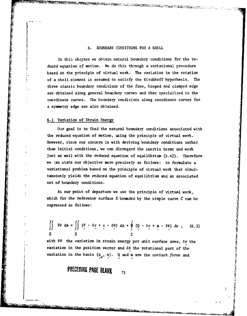
6. BOUNDARY CONDITIONS FOR A SHELL

In thi3 chzpter we obtain natural boundary conditions for the re-

duced equation of motion. We do this through a variational procedure

based on the principle of virtual work. The variation in the rotation

of a shell element is assumed to satisfy the Kirchhoff hypothesis. The

three classic boundary conditions of the free, hinged and clamped edge

are obtained along general boundary curves and then specialized to the

coordinate curves. The boundary conditions along coordinate curves for

a symmetry edge are also obtained.

6.1 Variation of Strain Energy

Our goal is to find the natural boundary conditions associated with

the reduced equation of motion, using the principle of virtual work.

However, since our concern is with deriving boundary conditions rather

than initial conditions, we can disregard the inertia terms and work

just as well with the reduced equation of equilibrium (5.42). Therefore

we -an state our objective more precisely as follows: to formulate a

variational problem based on the principle of virtual work that simul-

* taneously yields the reduced equation of equilibrium and an associated

set of boundary conditions.

As our point of departure we use the principle of virtual work,

which for the reference surface S bounded by the simple curve C can be

expressed as follows:

if6V da j(F -6r + c-66) da + (Q 6 + m 60) ds * (6.1)

S S C

with 6V the variation in strain energy per unit surface area, 6r the

variation in the position vector and 60 the rotational part of thevariation in the basis (a , n). Q and m are the contact force and

iPREEDING PAGE BlANK 71

-- __ ___

contact coupZe per unit arc length applied along the boundary C and, as

already mentioned, F and c are the external .=3rce and external couple

per unit area over the surface S.

The rotational part 60 of the variation in the basis (a , n) is

given by the expression

S 21 a ns = (aa x 6a + n x Sn) (6.2)

2- - - -

This expression assumes no dependence of 6n on Ea even though n is

normal to a a. We set up such a dependence by requiring that the vari-

ation in(a , n) satisfy the Kirchhoff hypothesis. Consequently the

variations 6n and Sa. must be such that the magnitude of n is unchanged

"This expression is easily derived by considering any vector • with

fixed components relative to the basis (a, n):

_a

6=ca + n 6 a" a 6 n n

Its variation due to varying (a , n) is

_a - - -a

and the rotational part of 66 is given by the antisymmetric part:

60 =- (Xa -a a a' + n 6•n-•n n)

from which the above expression follows.

72

= -.-- ~-A

- -- -ý - -M

and n remains normal to a dur-ing the variation, which gives us the

conditions

n - n = 0 , a - 6n + n • Sa = 0 (6.3)-. ~ _ a

Combining these conditions with the expression for 60, we have as a

consequence of the Kirchhoff hypothesis that 60 is completely determined

by 6a :

~lcL

6e a aax (6a + n n - 6a) (6.4)

Our aim is to find an appropriate expression for 6V; one which when

substituted in the principle of virtual work (6.1) yields the reduced

equation of equilibrium. We begin with the requirement that the princi-

ple of virtual work be consistent with the vanishing of the expression

6A= (Qa +F)- •6r + (m CE + a + c) • 60 (6.5)

Motivation for this requirement follows from the fact that 6A does

indeed vanish when the equations of equilibrium closest to physical

reality (5.5) are satisfied. Our analysis, however, does not depend

upon (5.5) being satisfied, but only on (6.5) vanishing.

A change in the order of differentiation in the last expression

gives

6A •(Q 6r + m - 60), + F - 6r + c - 60rCE

(6.6)- (Qa 6a a x Q*6t 8 + m a 66 0)

73

F

With the aid of (2.16) and (2.20), the derivative of 66 can be written

as follows

6j [n x as (by 6a - 2 6b + a x a 6r1TI (6.7)- t 2- - O -a ×L aY asV 67

which when combined with (4.24) gives us

m. .60l = baM y 6aB Ma6b . (6.8)

We also have from (6.4) the identity

a a6 aa - a xQ_ 6= es (6.9)_a -x a - . 2 a

In view of dofinitions (5.35) and (5.39), substitution of the last two

expressions in (6.6) results in

a a6A = (Q + m 60)a + F - 6r + c - 60

(6.10)6(aa6 a Ma 6 b a)

Integrating this euiation over the surface S and applying the divergence

theorem for surfaces, we obtain

fJ6Ada=I(Qa -6r+ma e) (F 6r+c.60)

SC (6.11)

- Jj' 6aae - 6b B) da

S

See Appendix A for a derivation of this theorem.

74

Comparison of this result with (6.1) shows that with

= 6a -Mas 6b , (6.12)

the principle of virtual work and the vanishing of 6A are consistent.

We have yet to show that this choice of 6V implies the reduced

equation of equilibrium (5.42), although the appearance in (6.12) of

precisely those mechanical variables occurring in the reduced equation

strongly suggests such a connection. Returning to (6.5), we use (4.24)

and (4.34) to replace ma and c by Ma and C, giving us

6A = + F] - 6r + [n x (Ma1 .+ C + a x (Qa - ba M 60 . (6.13)6A [ a -a - ] - -0 (.3

Using (6.4) to eliminate 60 and rearranging, this becomes

6A= [ + * F] • 6r - [(Msa n), + (Q (s) + b( Ma ala Y 3

(6.14)

+ Can n Qa] - 6a

SUsing the fact that 6a a---Sra to change the order of differentiation,

we obtain, in view of definitions (5.35), (5.39) and (5.40), the result

6A = [ + + a') + F] 6 r

(6.15)

Oa(( +)~ Q +Ca( [(M n) ,s 6 +° (i* -6 I r) C

Combining (4.24) and (6.4) to obtain

a .6- aBn6alm a So - M n (6.16)

75

k o-

and substituting this result and the previous expression for 6A in

(6.11), we obtain after rearranging terms the integral identity

fl 6 a 8 -M 6b ) da + J (M - + Qi C )~ + F] 6r daas s

S S

Sf(F - 6r~ + c:* 66) da + {[(M'a n),, + + r(.7

S C-Man n •a v ds

which on identifying 6V as per (6.12) becomes

JJ iSV da + JJ [(lMla+ Qa + Ca)1 + F]- 6r da

S S

- (F 6r~ + c* 60), da + s V~n) a + +~ r(.8s c {S C

- ma n 6a v ds

From comparing this result with (6.1), we conclude that the principle of

virtual work implies the integral equation

J*(W + F]- 6r da + S (Q ir + 6e 0) ds

S C (6.19)

S{[(M• n) + ÷ + - - -Cl 6 M n 6a,} va ds.

76

Since Sr is arbitrary, we first set 6r = 0 over S, giving us

6rQ- r m- 60) ds {[ n), + Q ] 6rc c(6.20)

- MrI8 n -Sa} v ds

It then follows from (6.19) that for arbitrary 6r

B a + Q- + Ea), + F] - 6r da = 0 (6.21)

S

Assuming that the integrand of this expression is continuous, the arbi-

trariness of 6r implies that the integrand itself must vanish, which is

clearly equivalent to the reduced equation of equilibrium (5.42) being

satisfied. Hence we have shown that with the choice of (6.12) -for 6V

the principle of virtual work does indeed imply the reduced equation of

equilibrium, and so (6.20) contains the associated natural boundary

conditions.

6.2 Classical Boundary Conditions aloi. aeral Curves

As it stands, expression (6.20) is somewhat unsatisfactory in that,

while the reduced equation of equilibrium (5.42) and the variation in

strain energy (6.12) depend only on the symmetric part of NI , it appears

that (6.20) involves W& entirely. We now show that this dependence is

spurious by first writing, without loss of generality, the antisymmetric

C part of M as

C= c ' M (6.22)

L

77

i

-I

It then follows that

f [(M[aal n) I" 6r -[•1 n • 6a% v ads

c (6.23)

= (M n - 6r), BC v ds

C

which by (A.9) becomes

4[(Mca I n),, - 6r -[8aI n • 6a] v ds

C (6.24)

=- (M n• 6r), ' T adSas

C

Since T is the unit tangent to C and satisfies

dr aT dE a (6.25)

we have as a consequence of M n • 6r being continuous that

f[(, [E•] n), 6r - M108 n •a ]v dsSC (6.26)

C f ý= - -(M n - 6r) as F-0( .6

-- dMn6sd~

C

and hence that (6.20) depends only on the symmetric part of Ma•.

78

Consequently, by virtue of (5.40) we can write

6r(+6 m -.66) ds f[( a1 + +C) - 6r -M Sa 1 v d

(6.27)

Because m has no normal component, see (4.21)2, we can assume

without loss of generality that the contact couple m also lacks a

normal component

m * n = 0 (6.28)

Hence, we can define the equivalent vector M:

M = m x n , m = n x M (6.29)

from which it follows that

S- 6e = - M - a n • 6a = - M n - 6a (6.30)

Substituting this expression in (6.27), we obtain

-W + ia + Ea - $a a;- ~

f .{ 1 - V - ~ Q 6r - [M~c v a- M ] n 6a lds 0

C (6.31)

The variation in a in the above equation cannot be independent of

6r because a - r,a . To isolate this dependence, we first observe that

Sby the Kirchhoff relation (6.3)1 6n cannot have a normal component and

hence can be resolved tangential to S along and normal to the curve C:

6n = T 6n + v v 6n (6.32)

79~ - . ~ ~

The component v • 6n represents a variational rotation of the normal n

about the tangent vector T and is independent of 6r in the sense that

v * 6n can vary arbitrarily when 6r = 0. Hence we write this component

as a rotation:

6= v 6n (6.33)

The component T 6n however is entirely determined by 6r, since

dr d6rS6n = - n - - n • = - n • --- (6.34)

With the last two expressions 6n becomes

d6r6n 6 v- n T -(6.35)

-ds-

and so by the Kirchhoff relation (6.3), we have

d6rn •6a, n • ds v 8 6ý (6.36)

Substituting this result into the boundary integral (6.31) and inte-

grating by parts along C, we obtain

~(I" V8c T Mc n T ) 6r

C (6.37)

Si+l[( -M V•)• 1 ds - [( v - M n) - 6 r 0,

i - - +S.1

wherein the last sum is over points i of discontinuity in the tangent T,

and hence in the normal v, and possibly in the applied contact couple

80

component M8 . Using the arbitrariness of 6r, we can separate the last

"equation; first setting 6r : , we get

S[(M _ ) ] 6V ds = 0 (6.38)I Cwhich when substituted back in (6.37) gives us for arbitrarY 6r

I(M + V + M n) T 6r ds

f 1 68 a +2]

C (6.39)

+ m [+(M v(3 M) - T - ](M-$ M ( B 8)1 n 6r= ,i

wherein we use superscripts (+) and (-) to denote the positive and

negative one-sided limits.

Using the boundary conditions (6.38) and (6.39) we obtain the

classic boundary conditions along a general curve C:

1. Cla•ped or cantiteverred edge, characterized by the position r and

the normal n being fixed along the boundary; hence along any portion

of the boundary that is clamped (6.38) and (6.39) are automatically

satisfied, since 6r =- 0 and 60 E 0, and we have along a clamped

edge

r = const. , n const. (6.40)

+)= lim S(s) and 6-= lim 6(s), cf. BUCK 116; p.79].

S4,s. sts.1 1I

SI

i~

2. Hinged or simply supported edge, characterized by the contact couple

M vanishing and the position r being fixed along the boundary; hence

along any hinged portion of the boundary (6.39) is satisfied, since

6r =0 . Assuming the integrand continuous, (6.38) will be satisfied

for arbitrary 6ý only if the integrand vanishes, so that along a

hinged edge

r = const. , Va v e = 0 (6.41)

3. Free edge, characterized by the contact force Q and contact couple

M vanishing along the boundary, edge displacements and rotations

being arbitrary. Hence, assuming the integrands continuous, (6.38)

and (6.39) will be satisfied along snooth portions of the boundary

only if

(Ma , , Cý ^a d a E(ti TS)v -, 0 , (6.42)

and at corners where T is discontinuous only if

6.3 Boumdarzy Conditions along Coordinate Curves

Along coordinate curves, where either ý1 or ý2 is a constant, the

free edge conditions and to a sr aller extent the hinged edge conditions

take on simpler forms. Let us first consider a l= const. coordinate

curve as a boundary. Along such a curve, the curve tangent t is colinear

with a2 and the curve normal v is colinear with al. Since T and v are

unit vectors, we have that

I= 0 T2 ±1 ' , 1 = 2l/,-' , =v2 0 (6.44)

82

-- - -- ~~-.

with the upper sign for the case when v and a1 have the same sense and

the lower when opposite. Moreover,St

T a12 T T 2 a 2 2 (2 d

Substituting these results in (6.41) and (6.42), we obtain for edge

conditions along 1 = const:

2'. Hinged edge ( c1 = const)

r = const. , 11 0 (6.46)

3'. Free edge (• = const)

M*il, 1 + 2 M*1 2 , 2 + *1= 0 , 11 0 (6.47)

wherein the starred variables defined by (5.44) and (5.46) are most

conveniently used. It is interesting to observe after writing the

reduced equation of motion (S.45) in extended foin

Y " 0 + Y*" I + [aa . (Y*C V + Y*2 E) n],E

(6.48)

=(*11,, + 2 M*1 2 12 + N*l),1 + (tA*22,2 + N* 2 ), 2 +

that precisely those variables differentiated with respect to 1 in the

- reduced equation arc the ones that vanish along the free edge.

83

1 _

- --

Next taking a 2= const, coordinate curve as a boundary, we have

= 1/a , z= 0 V1 = 0 V2 = ±1/1 2 2 , (6.49)

with the upper sign when v and a 2 have the same sense and the lower

sign otherwise. Moreover,

"Ti all Til T2 "rl T d 1 (65)a1

Substituting these results in (6.41) and (6.42), we obtain

2". Hinged edge (E2 = const)

r =const. , M* 2 2 -0 .(6.51)

3"1. Free edge g2 const)

H'22,2 + 2 M* 1 2 , 1 + N* 2 0 , M*22 = 0 (6.52)

Rearranging the reduced equation of motion (6.48):

*Z

t"O v + y*l w + [aa " (y*" v + Y*2 w) ]

:5$.53)

=(*22, + 2 M*1 2 ,1 + N* 2 ), 2 + (M*l•,1 + ]*1),+ F*

we again ob:erve that the variables differentiated with respect to E2

vanish along the free edge.

84

F1

When a boundary coincides with the intersection of a 1 = const.

Sand a E2 const.coordinate curve, then the free edge condition at•' corners (6.43) holds, giving us in addition to conditions (6.47) and

(6.52) the condition

3'". Free corner (l = const & r2 = const.)

M.I2 = 0 (6.54)

6.4 Symmetry Boundary Conditions

A syninetry edge or boundary is not a physical boundary of the shell,

but is a middle surface curve that always lies in a plane about which

the shell deforms symmetrically. Hence, initially and for all, subsequent

positions, this plane will be a symmetry plane of the shell. It is con-

venient to take the symmetry boundary as a coordinate curve and to have

the remaining coordinate curves symmetrically distributed with respect

to the symmetry plane. Also the external force F and external couple cmust be symmetrically distributed.

Let us first take the symmetry edge to be the El = coordinate0

curve. Also let the synrmetry plane be located a perpendicular distance

K1 from the origin, and oriented relative to the constant orthonormal

basis k. (i = 1,2,3) such that k1 is normal and hence k (a = 2,3)

parallel to the plane as shown in Figure 6.1. It then follows that

when El = " the position vector lies on the symmetry plane, so that0 '

r (IC, E2, t) k = K, (6.55)

Moreover, using the simplifying notation

f+=f(El + E, E2), Lý_ E E°_ :• 2), ,. , (r, &2),00 '0

85

• ;F•%> •• .•.•_•------ = ----------.-----------.-.---. ,.... , *_

PLANE

k_

< k, K,

10

Figure 6.1 Deflection pattern of the middle surface of a shell

deforming symmetrically about a symmne'ry plane. The intersection of

the symmetry plane and the middle surface is the symmetry boundary,

for which material coordinate is a constant El = '. The symmetry

plane is a perpendicular distance K, from the origin 0 and normal

to the vector k, of t;.ý constant orthonormal basis k..

86

we have, as a consequence of the coordinate curves being bynmmetrically

located with respect to the symmetry plane, that

(r÷ + r ) k = 2 r • kj = 2 K1 , (r÷ - r ) - k = 0 (a = 2,3).

(6.56)

With these relations, we obtain in Appendix B the symmetry properties

of the basis vectors, normal vector, metric, etc. and combine these

results with the velocity relations, strain relations and resultant

relations co obtain the symmetry properties of the variables appearing

in the reluced equation of motion (5.45):

(a- - aj k 1 = 0 , (al + a1 )- • k= 0

(a2+ a 2 ) - k, =0 , (a 2 - ) - k =0 (6.57)

(n+ n) k = 0 , (n+ - n_) • k = 0

(v + v_) - kj = 0 (v+ - v_) - k• = 0

(W+ + w•) - ki = 0 , (W+ - w_) " k = 0 , (6.58)

(F* + F*) k,= 0 , (F*. F*) - k(; 0

M*II = M*11 m*12 = - M.12 M.22 = M*22+ ÷ - + J

Q*.ll Q*,I Q*. 2 = _ Q*12 + -, , (6.59)

N*I= - _ , =N*2

87

Clearly, the above symmetry relations hold at positions symmetrically

located with respect to the boundary and are useful in the finite differ-

rence formulation of the reduced equations of motion along symmetry

boundaries. These relations can be also be used to obtain the conditions

on these variables and their derivatives at the boundary, for observe

that as, A - 0 , we have that 6+ - 6 and 6- - j . When we use this

fact and note that a, and al at the boundary are colinear with k, we

find that

v1 = 0 , W1 = 0 , F*I = 0 , %*12 = 0 , Q* 1 2 = 0 , = 0 (6.60)

Next, taking thL- symmetry edge to be the ý2 =2 coordinate curve,0

we locate the symmetry plane at peipendicular distance K2 from the

origin and orient it relative to the basis k. such that k 2 is normal and

hence k (T = 1,3) parallel to the plane. With the notation~ T

(El, E2 + A. 2 ) 6 = (, C1 2 - A02) , 1, E2)

we then have that the position vector satisfies

(r+ + r ) - k2 = 2 r - k 2 = 2 K2 , (r, - r ) -k = 0 (T = 1,3). (6.61)

As shown in Appendix B, with these relations we obtain the syimetry of

the variables appearing in ,'5.42):

(a 2 - a2 ) • k 2 = 0 , (a 2 + a 2 ) * k = 0

(al + al) _ k 2 = 0 , (a+ - al) - kl = 0 , (6.62)

(n+ + n_) - k =0 , (n+ -n) k=0

88

I(v+ + v ) k2 =0 , (v -v) k =0

(+ + ,,_) • = 0 , (W - w_) • k = 0 , (6.63)

*+F*)_ -k 2 =o , (F* F*) k . C(*+ F)- k + T-

M *1 = _.i *1 m*22 = _ 2"+- -- -+ _

Q* =Q1 *1 = _-*1 Q* 22 = Q*2(6.64)

N*l=N*1 * *

When we take the limit as A.2 - 0 , using the fact that at the boundary

a 2 and a 2 are colinear with k 2 , we find

V2= 0 ,W2 0 , F = 0 , , Q*1 2 = 0, N*2 = 0 (6.65)

89

7. MATHEMATICAL FORMULATION OF THE REPSIL CODE

in this chapter we begin by specializing the general shell theory

developed in the previous chapters to the theory on which the finite

difference formulation used in REPSIL is based. This specialization is

accomplished in two steps: first the thin shell approximation is applied

to the general equation and then further restrictions, both physical and

mathematical, are imposed to yield the special theory on which REPSIL is

based. The chapter concludes with a deszription of how this theory is

implemented in REPSIL and of the computational procedure used to obtain

a solution.

7.1 Equations of Thin Shell Theory

The theory developed in Chapters 2 through 6 assumes only that thz

deformation undergone by the shell satisfies the Kirchhoff hypothesis.

As noted on page 29, this assumption entails a mild restriction: the

deformation must be such that the minimum principle radius of curvature

is greater than half the thickness; i.e. < R Otherwise, the

position of particles would not be unique.

We now impose a more stringent restriction on the deformation bya2

requiring Rmin be so much larger than h that terms of order 1; bal and

higher can be neglected and dropped in comparison to u-iity. In other

words, we assume that for sufficiently thin shells thest higher order

terms have little affect on the deformation. The resulting equations

we call the t.hin shell equations and the resulting thecry - thin shell

theory. The theory developed here differs from the classical theory of

thin shells, in that the latter neglects terms of order ký bBI in all but

the expressions for the strain . This difference will be pointed out

in the development.

A clear and straightforward exposition of classical thin shell theoryusipg the Kirchh:ff hypothesis is given in [13; Ch. 2]. Directcomparison of tha classical equations as set forth in this referenceand the equations of the present work is however made difficult by theunnecessary use of principal curvature coordinates in the former.

PRECEDING PAGE BLANK 91

9 -

We will be mainly concerned with obtaining the thin shell versions

of the equations associated with the reduced equation of motion (5.45),

which form the basis of the REPSIL formulation. The specialization to

thin shells of equations associated with other forms of the equations of

motion is however straightforward.

Relations involving the geometry of the middle surface will remain

unchanged. Only geometric relations off the middle surface will be

altered by the thin shell assumption, due to their dependence on ý ba

through the variable v a being made linear. Hence, while the metric a8 as8

is unchanged, the metric gas given by (2.46) becomes

g = a a -2 g ba8 . (7.1)

It follows from (3.12) that the incremental strain-displacement relation

(3.20) also becomes linear in •:S~1

AEa8 :y(a Au,• + a • Au, a- Aua . Au, )

(7.2)-2(n - Au, a - An • a - An Au )]

For computational convenience, tue REPSIL formulation, rather than use

the last form of the strain-displacement relation, uses the equivalent

but shorter form

AEaE 8 -[(a- Au, + a Au, -Au, *La- -a a

(7.3)- 2ý(n- - Au, as + An a a's)] .

The surface normal-displacement relation (3.30) is unaffected by the

thin shell assumption.

Since all the resultant relations of Chapter 4 are obtained by

integration through the thickness, they are all altered. In particular

for the zeroth, first and second resul- moments of mass density

(4.15), we now have

92

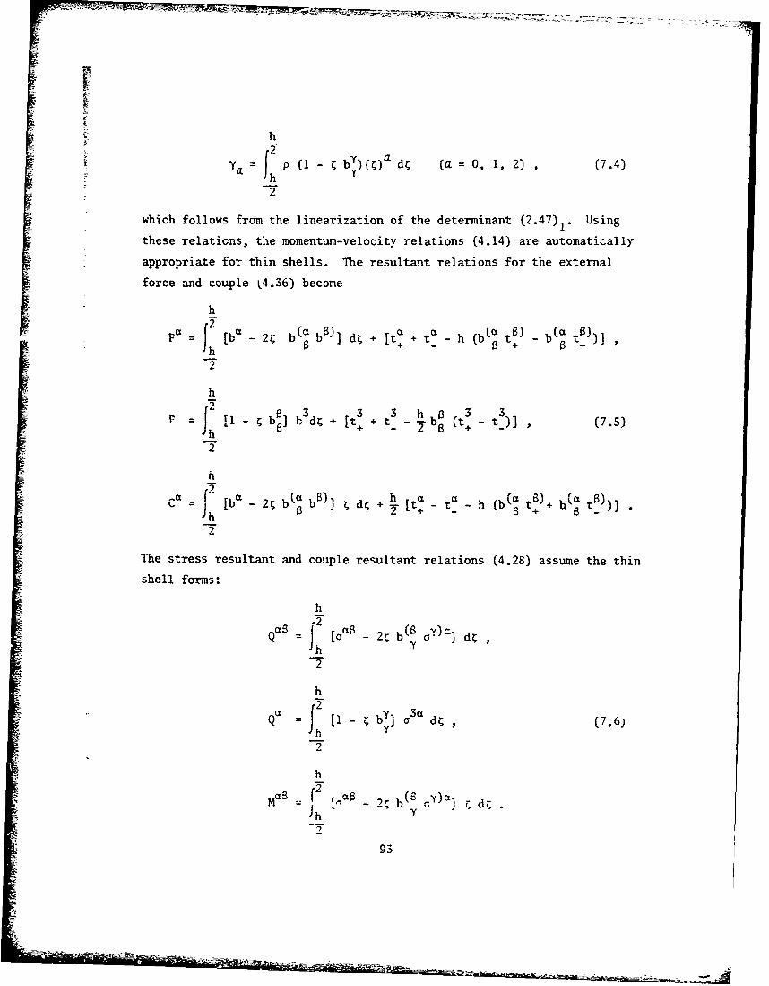
hy= p (1- by (,)a d (a O, 1, 2), (7.4)

a hY-h

• 2

which follows from the linearization of the determinant (2.47)1V Using

these relations, the momentum-velocity relations (4.14) are automatically

appropriate for thin shells. The resultant relations for the external

force and couple i4.36) become

h

F a 2 [" 2ýb ( 0]d4 [t"i + tc' h- bf a at6=2 bi- 2 b] + +h( b )~ _ b' tB

h + +

2

h

[I b bU+ +3 t hbt (t+2 _ t))] (7.5)-h

. 2

h

-a 2 [ba- 2d b (a 0 h [+_ L ttah t+ )+b(a _t))]S• = Jh 2 d +- + -a b• B)

The stress resultant and couple resultant relations (4.28) assume the thin

shell forms:

h

Q a5 =2 [oa as_ 2; b(B Y• dý(- h Y )

h

-1 by] Sa dz , (7.6)

h

. 2 ,cas - 2ý b(S cy)al d,Jh "Y

-5-

93

However, of more direct concern to the RErSIL formulation are the thin

shell forms of the resultant relations for the modified membrane and

bending components:

h

Qa 2L [1~ by] a asdý

(7-7)h

f 2 [(1 b y ) a a b (a aba)] d4 ,h yv y

which follow from (5.43). With the above thin shell expressions for

YO, Yl, Y2, Fa, F, Ca, Q6 and M , the reduced equation of motion (3.41)

or (5.45) is appropriate for thin shell theory without need of change.

As mentioned before, classical thin shell theory goes further by

dropping the linear terms in (7.1), (7.4) - (7.7), giving us the

approximations:

h2

g =aaB ()ad a (=o, 1, 2),

h h

gasa ata 1h Y-- 7h h

Qa 'a aJa-"dr2 ih-t3 t

F• b• dý + t+ + ta F b bdý + t+Jh + -h -'

2 2(7.8)

h h

Caa ^ a CL 2 3a

-f -7

94 "

22

h h

Notice that the distinction between components Q & M and themodified components B M disappears completely in classical thin

shell theory. Moreover notice that if the linear terms in the strain

expressions (7.2) & (7.3) were also dropped, then the strain would not

take into account bending and so would be appropriate for membrane

theory . In any event, the theory forming the basis for the REPSIL

formulation retains for the sake of consistancy terms linear in b

in the membrane and bending components.

7.2 Restricted Thin Shell Theory Used by REPSIL

The equations on which the finite difference scheme used in REPSIL

is based are simplified forms of the thin shell equations just developed.The simplifications are of two types: the first arise from the specifictype of problems that REPSIL is designed to treat and the effectspredominating therein, with no mathematical approximation being used.

The second follows from the mathematical need to make the equationssimpler to solve, and involve approximations. Also, we adopt anelastoplastic constitutive relation between stress and strain to make

the formulation complete.

REPSIL is formulated to treat the large transient response of thin

shells subjected to blast loads. For this reason the surface tractions

are assumed to be predominantly due to blast pressures, with the effectsof viscous drag being nil. Moreover, the effect of gravicy through thebody forces on the deformation is negligible com-ared to the b.ast

pressure effect. Hence, the traction and body force fields have the

special forms:

t P n t =P n , b 0, (7.9)

Memb-ane theory is treated in [12; Sect. 14.3] and [13; Ch. 4).

95

which when applied to the components of F and C as given by (7.5)yield

h 8F- [P- P - b (P + P ) n , C = 0. (7.10)

The shell is assumed to be initially homogeneous, so that the initial

mass density p0 is constant. Hence, expressions (7.4) for the resultant

moments of mass density can be integrated for their initial values,

which givesr0 =P h1 By P h3 r2 1 h3,

0 , rl 1 =--• B • =.1-Ph (7.11)

Consequently, from (5.20) we have

S1 L B o h3 A½ i h3 A2.(7.12)y*0 = po h A½, yl B p h- A , *2 =•o01 y o Y 2 0~~

As mentioned earlier, the first resultant moment of mass density is a

measure of the distance from the middle surface to the cencer of mass

for the section. It is clear from (7.11)2 that for an initiaily uniform

thin shell, the center of mass will coincide with the middle surface

when the initial geometry of the shell is such that the mean curvature

By vanishes, which is tantamount to the principal radii of curvature

being equal but oppositely directed. It then follows that the first

resultant moment of mass density will vanish for all subsequent time,

even though the mean curvature by may no longer vanish. In particularY

this holds tr-e for initially flat shells.

Expressions (7.10) - (7.12) are exact within thin shell theory.

For the sake of simplicity, we now go further and assume that the first

order terms can also be neglected in these expressions:

F=- [P P ]n =- pn, C= 0,

ro h F1 0 r2= h2 ho (0. 1 0½

Y*O Poh Aa 2 h* Y 01= 2 , y*i = 0 , Y* 2 = h 00 ,

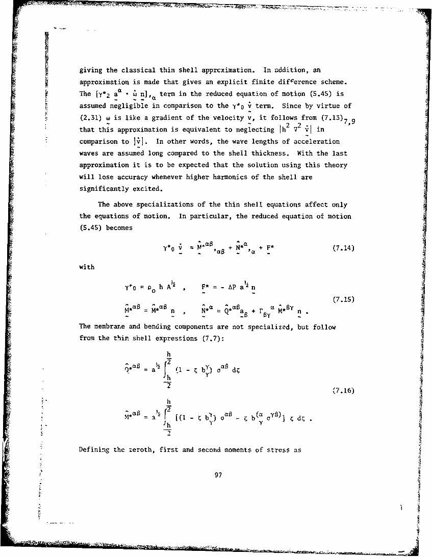
giving the classical thin shell apprcximation. In addition, an

approximation is made that gives an explicit finite difference scheme.

The [y"2 a • ~ n], term in the reduced equation of motion (5.45) isassumed negligible in comparison to the y*0 ~ term. Since by virtue of

(2.31) w is like a gradient of the velocity v, it follows from (7.13)7,9

that this approximation is equivalent to neglecting 1h2 V2 •, in

comparison to . In other words, the wave lengths of acceleration

waves are assumed long compared to the shell thickness. With the last

approximation it is to be expected that the solution using this theory

will lose accuracy whenever higher harmonics of the shell are

significantly excited.

The above specializations of the thin shell equations affect onlythe equations of motion. In particular, the reduced equation of motion

(5.45) becomes

Y*O = M''a + N + F* (7.14)

with

Y*0 = h0 2 A F* = AP a n_ (7.15)* as ja as ar ý.*Y

n a, + r-y

The membrane and bending components are not specialized, but follow

from the thin shell expressions (7.7):

h

;*.• =a½ a (1- 1 b') oa d;

h

= ½j [-- -• a - bU&~)~d~h(2

Defining the zeroth, first and second moments of stress as

97

1 A

- <- - - - § -~' -I

h

2Ea f a(C'dý (az=0. 1, 2) (7.17)

-7

the last two relations can be expressed as:

*.as =1-_ a 6 [ -by &Is0 Y 1 0 y-8

(7.18)

ý.aB = a2 [2X - by zE' - b (a Eye)1 Y 2 Y 2

In order to complete the formulation it is necessary to specify in

what way the stress is related to the strain. Before doing this, we

first characterize the stress field by assuming that a state of plane

stress exists in each lamella parallel to the middle surface and that

the shell is :omposed of isotropic material. However, for an isotropic

material the strain components given by the Kirchhoff hypothesis, see

equation (3.6), are inconsistant with the plane stress assumption, since

the vanishing normal strain component %ill usually result in a non-zero

normal stress component. This situation is resolved in the usual way by

using the Kirchhoff hypothesis to determine only the tangential

components of strain, with the normal components following from the

plane stress conditions.

Presently, the REPSIL formulation employs an elastoplastic stress-

strain law that is linear in the elastic range and is capable of

modelling strain hardening and strain rate effects through the use of

the mechanical sublayer model . Using the above assumptions we derive

in Appendix C an expression relating the incremental change in the stress

components to the components of the strain increment and the present

values of the stress components:

AE• EI-A A l-4v c oy , (7.19)E A + , 6, &EY - AX [a - 1 -V 7. 9

See [2; Sect. 5.4.2] for a comcise description of the mechanicalsublayer concept.

98

wherein the mixed components are with respect to the basis g

Ac g= Aa 0E a =gY C . (7.20)

The factor AX is non-negative and its value is determined fromn the

von Mises-Hencky yield condition:

Sa - 1 (a )2 2 2 < (7.21)

with a the uniaxial yield stress. When AX = 0 in (7.19) results in a0

state of stress a + AOa outside the yield surface 0(aa + Aa) > 0, then

the proper value of AX is the smallest positive value that satisfies

ý(y'+ Aoc) = 0. Otherwise, AX = 0 is the proper value since it gives a

state of stress on or within the yield surface 0(o8 + AU ) 8 0. Thevalue of AX is thus determined by (7.21) and the stress increments (7.19)

are completely specified. For a strain hardening material the stress

components and yield stress pertain to each mechanical sublayer. A

procedure for dealing with the possibility of complex AX has been

developed in [4] and is presently incorporated in the REPSIL code.

7.3 Description of the REPSIL Formulation

We give a description of the computational procedure employed in

the REPSIL code, including an outline of the algorithm used to advance

-*the solution one time step . The computational procedure is similar to

that used in PETROS 1 and 2, so that the following description will

facilitate the comparison of these codes in the next chapter.

Basically all these codes solve finite difference forms of partial

differential equations that characterize the transient deformation of a

thin Kirchhcff shell. Finite differencing with respect to the materiala

coordinates E results in the dependent variables of the theory beingdefined on a two dimensional Lagrangian mesh or grid of points. At

A detailed description of the REPSIL code and its computationalformulation will be soon forthcoming in a user's manual.

99

interior mesh points and at those along symmetry boundaries central

finite difference operators are employed, while along fixed boundaries

(either hinged as clamped) forward or backward difference operators are

used, with all operators being of order IAt=I 2 . At present the

Lagrangian mesh has a rectangular boundary, which means that the REPSIL

formulation is restricted to shells having simply connected middle

surfaces bounded by four smooth arcs.

The shell is conceptually divided by a number of lamellae

parallel to the middle surface into K layers within which the strain

components are assumed constant at their mid-layer values, making thestress components similarly uniform. The reason this is done, despitethe fact that the strain increments are simple linear functions ot

as can be seen from (7.3), is that plastic flow soon makes impossiblethe simple analytic characterization of the .ariation of the stresscomponents through the thickness. Thus, the components of stress andstrain are defiied at stations k = 1,...K through the thickness, as well

as at each point of the Lagrangian mesh. This dependence on k will notbe explicitly indicated in what follows.

Replacement of time derivatives in the shell equation by their

equivalent finite difference operators results ii, an explicit finitedifference scheme characterizing the manner ir. ,hich ehe dependent

variables of the shell change during a time intLrai A*. Hence knowing

the values of the shell variable at time t, we are able to calculate

their values at the time t + At. The finite t..ne derivatives employed

are centered and of order jAt 2. The interval At does not change with

time, but is fixed at a value for which the explicit finite differepce

scheme is stable.

Before a calculation can begin, the material properties and theinitial geometry of the shell must be specified. An initial velocity

and/or initial pressure distribution starts the calculation, giving the

A finite difference formulation of the free edge conditions has yetto be added to the REPSIL code.

100

EFinitial chaisge that the shell variables undergo. After that a sequence

of calculations are repeated cyclically, using when appropriate

pressure-time data, to generate later and later values of the ,iell

variables progressively until some presciibed maximum time is reached,

at which calculations terminate.

With the above brief description of the finite difference

formulation and computational procedure employed in the REPSIL code in

mind, we are ready to describe the algorithm that forms the heart of the

sequential computations advancing the solution one time step . To keep

this description simple we shall not izeat a strain hardening or strain

rate sensitive material, although as mentioned earlier REPSIL can treat

materials exhibiting such phenomena. The algorithm is a recipe for

solving the set of algebraic equations that result from finite

differencing the shell equations. For our purposes, it is sufficient

to exhibit the finite time derivative explicitly, continuing to

symbolize the difference operators with respect to a by partial

derivatives

Let us assume that calculations have progressed n-l time steps to

the time t = (n-l) At and that the position vector r and normal vector

n are known at each mesh point and the stress components a are known

at each mesh point and station through the thickness. Also the

displacement increment Au for the time interval t = 1) At to

t = n At is assumed to have just been calculated at each mesh point.

Using the notation

A less detailed description is pre:ented in a recent report[5; Sect. IIJ.

€ **

The piecise finite difference expressions will be in the forthcominguser's manual.

"101

-

-K ~ ~ ~ M MT ; T -L -z.z:-:

6 [(n-l)At] , 6 = 6 [nJt] , 6+ 6 [(n+l)At]

A =6-6- , A+="6 _4 1,*

our objective is to outline the sequence of calculations by which the A0, +Anew values r, n, ca Au of the shell v.•riables are generated from the

previously known values r, n-, u-as, Au. This sequence basically

involves five calculations, performed in the following order:

7.3.1 Current Geometry Calculation. The current position vector

r is found from (3.11):

r =r-+ Au... . (7.22)

Finite differencing the current position vector r gives the variables

characterizing the differential geometry of the middle surface (see the

equations of section 2.2):

a = r, , a =a • a,

a = all a 2 2 - (a 1 2 ) 2 n = al x a2 a

all a 2 2 /a a12 = - a12/a , 22= all/a , (7.23)

b =n-ra , b 8 = a8 y b

a a a, r ~ ay -r,.as a

7.3.2 Strain Increment Calculation. In order to determine the

strain increments, it is first necessary to find the incremental change

in the surface normal by finite differencing the displacement

increments Au and using (3.30) and (3.31):An

--An n •Au, An= [ + ]a A (7.24)

a l+nono a n (2

Notice that this notation is in accord with that employed earlier inSections 3.2 and 3.3.

102

The strain increments through the thickness at stations C(k), k 1 ,...K, AI are calculated from the thin shell relation (7.3): u

AE =- (a Au, + a Au, - Aua .AU

as 2 (a a~a -P

( A) (7.25)S - • (n- Au, ^+An - r,aB

Notice that the formulae for An and AfB are at least linear in Au,assuring numerical accuracy by circumventing the need to take differencesof nearly equal terms.

7.3.3 Elastoplastic Stress Calculation. The stress calculation

uses mixed components of stress and strain. Hence, it is necessary toasknow the metric gas and inverse g at stations z(k) through the

thickness. These follow from the thin shell relation (7.1) and the

equations of section 2.3:

gas = a as - 2 C b B , g = gll g 22 - (g1 2 )2 (

11 12 2(7.26)gl11= 922/g P g 12 91 g2/g , g 22 = g11/g •

With these relations the miyed com-ponents of the strain increment and

the stress are obtained:

AE'- = galy AE aC- ~ -a(.7

Next, the components of the elas..ic stress increment

E aACT [A + , AE 6'] (7.28)8 l+V 8 1-v Y 8

and the plastic flow corrector stress

Ca -a I - (7.29)1 -CF a a 8 3--1--v) a 6 8(.9

are determined and used to find the current values of the stress

components using (7.19):

103

I

g __---_ _ _

-IlT C0a8= a8 - AO 8,, (7.30) a

with

T Ea -ai ai

a= 8 a A (7.31)

TThe value of AX depends on 08 through the yield condition (7.21). WhenTa is on or within the yield surface

Ta T 1 y22 = a(2 (7.32)B a -- (o -3

ci4

Tthen A•X =0 and current stress components are a• otherwise, AX• is the

smallest positive value giving a current stress on the yield surface

a 8 1 y 2 22a8 -r T (a) = = a (7.33)

a 40 Y 0"

In either event a value for AX and hence the values of a0 are determined.

Finally the contravariant components of the stress are found

as8 ay 8oaB ag 0 (7.34)Y

When the value of AX is complex, a procedure developed by H-lFFINGTON [4]

is used to determine the stress. As pointed out in Appendix C, the

stress calculation is not exactly centered with respect to time due toC

the use of a to calculate 08

7.3.4 Membrane and Bending Resultants Calculation. The zeroth,

first and second moment of stress are determined using (7.17)

= •~ c A(a = 0, 1, 2) (7.35)k

wherein the summation sign over k is used to emphasize that numerical

integration through the shell thickness is involved. With the above

values of stress m'-tnts, the membrane and bending components follow

104

from the thin shell relations (7.18):

* = as [r - b7 a1Q ~ 0 b Y I

(7.36)

.a a½ [I b• Eas - b E8)]S Y 2 Y2

7.3.5 Equation of Motion Calculation. Using the just determined

values of .* and M*. and the a priori specified values of the

pressure differential AP between the shell faces, the vectors

• •.a = s a. a, + AA- .vN* M* na ,

"(7.37)

14* =14_ n F* = AP a n

are dttermined (cf. (7,15)), The finite difference form of the

equation of motion (7.14) with the above volues gives the displacement

increment Au for the next time increment:

2AAu Au + (At) [ as + N +* (738)

. . a,*

wherein y*0 is the initially determined time constant

2-IYO P0 h A (7.39)

This calculation completes the cycle, the current values r, n,c8 + -4cz

"a , Au having been determined from the previous values r-, n-, a ,

Au. Hence, the solution has been advanced a time step from t = (n-l) At

to t = nAt. Repeating this sequence, the computer code generates later

and later values of r, n, a Au until some prescribed maximum time

t NAt is reached.S~maxL 7.3.6 Energy Balance and Strain Calculations. The sequence of

calculations just outlined is vital for the advancement of the solution.

Concurrent with this sequence there are performed calculations that,

although not essential to the solution, do provide information about the

current state of the shell. More specifically, as a global measure of

105N a

IN

the deformation, the work done by the pressure, the kinetic energy and

the elastic strain energy are calculated for each time cycle. The

difference between the pressure work and the sum of the kinetic and strain

energy indicates the amount of energy degradation caused by plastic flow.

Also, as a local measure of the deformation, the physical components of

strain at selected points on the bounding surfaces of the shell are

calculated for each time cycle. These components are exact for large

strains. The e4uations employed in the REPSIL code for the strain

calculations are derived in Appendix D of this report. The derivation

of the equations used for the energy calculations is reserved for a

subsequence report. The forthcoming user's manual will describe how

both the energy balance and strain equations are implemented in the

REPSIL code.

106At

8. COMPARISON OF THE REPSIL, PETROS 2 AND PETROS 1 CODES

As mentioned in the introductory chapter, the REPSIL and PETROS 2

codes are developments of the PETROS 1 code, both correcting and

generalizing the PETROS 1 formulation. In this chapter we compare the

theoretical and computational capabilities of these codes. First the

theoretical formulations used in these codes are compared and it is

shown how the theory on which PEiROS 1 is based has been generalized

and made less restrictive. Next the computational improvements and

increased capabilities of REPSIL and PETROS 2 over PETROS 1 are

qualitatively compared. The results of these comparisons are

summarized in tables and the implications ot the differences between

these codes are discussed briefly.

8.1 Comparison of Theoretical Formulations

The REPSIL, PETROS 1 and PETROS 2 codes are based on theories that

are quite similar. All assume the Kirchhoff hypothesis to hold and all

restrict therAselves to thin shells. Often the formulations of these

codes are based on the same equations. Essentially all employ the same

formulae to describe the differential geometry of the middle surface.

They Uiffer principally in the equations on which 10 the strain

increment calculation, 20 the elastoplastic stress calculation, 30 the Amembrane and bending resultant calculation and 40 the associated

equation of motion calculation are based (cf. Sections 7.3.2 - 7.3.S).

We will discuss these differences in this order, combining the last

two.

8.1.1 Strain increment Formulation. The various strain-

displacement relations employed in these codes have as common bases

the Kirchhoff hypothesis and thin shell assumption. The precise fonns

of the relations can be summarized as follows:

107

-24

12

7F

IC! REPSIL (cf. (7.24) & (7.25)):

AE (a AU, + Au, Au, *Auas 2 -C' - -8 A-a u5

A(n Au,,, + An • r, *) ,- ~- - (8.1)

a as An AnAn =- n Au, , An = -" I~+n-n-

PETROS 2 [2; Eq. 6.18, 5.23 & 5.29)]:

AE =-(a. Au, +*A .Au, -Au, O-Au,

2- (n -Au, 8 An * r,- An Au, o.8_ '(8.2)

An = a= AnAua

I PETROS 1 [1; Eq. 3.46 & 3.40):1

AE !-[(a * Au, +a Au,) + (a on, a An,aS 2 -.a .8 ..a8 a -.a 3 -84~ na)

Ana = n -n Au, - , Au , An 0 A3)

with An & An being the components of An for all three formulations:

An =An a + An n. (3,J)a.

From (3.16), it is clear that PETROS 2 uses an expression for AE. {&,

that is exactly equivalent to that used by REPSIL. Also, both use the

same expression for An The substitution of (3.16'2 in S8.) gives a

quadratic equation on An of which (8.2)3 is the solution under the mild

condition n * n > 0, so that both REPSIL and PETROS 2 use equivalent

expressions for An. Hence, REPSIL and PETROS 2 have equivalent strai.n

increment fcrmulations.

108

-L4*•_-- _ . _ -= - -__-

In order to compare the expression for AE used in PETROS 1, we

need to commute the order of differentiating terms in (8.1)I using

(3.24) to obtain the

• • ~ ~~AEa 1 •u•+ ••E a E -[(a a +a Au, - Au Au, 8 )

+(a - An + a An, + n, •Au + n,• Au• (8.5)

A-n, *Au -An, Au,)]S~a ~B 2$

When this expression and the REPSIL expressions for the components of

An are linearized by neglecting products of gradients of the displacement

increments, there result the equations

AEa 2 [( * Au, +a *Auil)

+ An, + a An, n, • .u, + n . Au, A)a 28 8 -a a ~8 2

S~(8.6)An = - n Au, S An = 0a

These equations would coincide with the PETROS 1 expressions for AE IAn & An if the term n, were negligible, which means that the middle

surface would have to remain virtually flat. Hence, PETROS 1 uses an

approximation to the exact REPSIL strain increment formulation which is

valid only when displacement gradients are small and the shell is

virtually flat throughout the deformation. Consequently, for the

particular shell geometry treated by PETROS 1, a cylindrical panel, it

cannot be expected to give good results.

8.1.2 Elastoplastic Stress Formulation. Both the REPSIL and

PETROS 2 stress formulations account for the variation in the metric

through the thickness, while the PETROS 1 formulation disregards this

variation. Specifically, these codes use the following formulae for

the metric and inverse:

[ 'Z

Notice that this expression is equivalent to the R"' expression forAE in the partial differential sense, but not zhe finite differenceas

S sense.109

PK- , T.. . ..

REPSIL (cf. (7.26))

gas a 2h , g = gu1 g2 2 -(12

(8.7)g12 22 t

g = g2 2 /g , - g12/g , 92= 1g'l/ ,

PETROS 2 [2; ,q 5.106 & 5.1071)

ga s - 2a ba , g = a + 2u b (8.8)

PETAOS 1 [1; Sect. 5.1.2] c 2

=Ag = A a B = as (8.9)

The ioxr- a, -or ga,: used by REPSIL ind PETROS 2 are identical and are

'ased , -•' itin shell assumption. On zhe other hand REPSIL employs

the ex",, iverse g to gas while PETROS 2 uses an approximate thin

shell inverse. PETROS 1 implicitly assumes that the metric and inverse

ie equal to the initial middle surface metric and inverse, which for

the particular initial geometry treated (the cylinder section) equal

the Krc, •cker delta. Hence, PETROS 1 becomes more restrictive than

either REPSIL and PETROS 2 by assuming the .. assical thin shell

approximation and neglecting any variation through the thickness

(cf. (7.8)1) Moreover, the distortion of the middle surface is

neglected. Thus, PETROS 1 uses an approximation to the thin shell

expressions used by REPSIL and PETROS 2 for the metric gas and inverse

g , which is valid for extremely thin shells that suffer negligible

middle surface distortions.

REPSIL and PETROS 2 employ mixed components in their expressions

for determining the stress, while the PETROS 1 expressions do not

distinguish covariant from contravariant components due to the special

form of its metric. However, for the sake of comparison we shall also

write the OETROS 1 expression in mixed components, summarizing the

expressions used by these codes for determining the stress as follows:

110

_ '

REPSIL (cf. (7.28) - (7.31), (7.33))

Ta a 13 + + ( 1'A

C - 1-2v -y a(8.y

a C Ft 8 8 3(1-V) y a'(.0

T Ca -a X a AX2 -2B AX + C 0,

PETROS 2 [2; Eq. 5.68 - 5.75]

T EySo -a + 1 (AEa +--AE1 6'

C T Ta 1a 1-2v (.1

= 6 , (8.11)8 'B 3(1-V) y

T. C2

PETROS 1 [1; Sect. 4.3]

a t a O aSoB=a + T (AEB +i'~E -) ,a -aB a V

Ta _ a 1-2v Ta 3(1-2V) 'y (8.12)

T CaB o -AX a -2B AX + C =0,

where mixed components are given by (7.27) 4 (7.34) and the coefficient

A, B, C are defined uniformly as

-C C CCa 8 1 Ca 8B

A a 3 a 8 '

CT OCTC T I C aT e

T T 1 TaT0 2 2C aB 1 ~aB- o -2Co 8 a 3 0 0

if0

in all the above formulae. The first difference to be noted in these

formulations is that wMhle REPSIL and PETROS 2 determine AX from the

exact quadratic formulae thus assuring a stress ac on the yield surface,

PETROS 1 uses a linear approximation to determine AX giving a stress not

necessarily on the yield surface. HUFFINGrON [4; Sect. V] has assessed

the possible errors resulting from the use of this linear approximation,indicating that in a typical problem involving the large transient

deformation of a cylindrical panel on tne average a discrepancy of 50%

in the stresses can occur which initially can go as high as 210%.

Hence, we can conclude that the use of a linear approximation for AX

in this type of problem is certainly inappropriate.

A second not so obvious difference involves the stress componentsc a

used to determine corrector stress components ao, PETROS 1 andT T

PETROS 2 using a a instead of a-a as REPSIL does. The use of ao' is

rationalized in [2; Sect. 5.4.3] by the observation that a real value

for AX is more likely to result by its use. However, this ad hoc

reasoning becomes much less persuasive when it is realized that theTa

plastic flow rule (C.10) is violated by this choice, because aa lies

outside rather than on the yield surface. When we add to this the

fact that the procedure using o-a outlined in [4; Sect. IV] and used in

REPSIL has proved in practice completely adequate, giving real AX forT

all reasonable deformations, the choice of a become still less

justified.

Lastly, we point out that all three codes have the capability of

treating strain rate sensitive and strain hardening materials, and do

this in more or less the same manner using a mechanical sublayer model

for strain hardening and an exponential strain rate dependent yield stress :i

[2; Sect. 5.4.2].

8.1.3 Equation of Motion and Associated Resultants Formulation.

The various forms of the equations of motions used by these codes are

limited by the common assumptions that

112

c=0 , Y1= 0 , Y2= 0. (8.14)

Hence, comparison of these equations will be within the limits imposedby these assumptions. The equations of motion and the associated

membrane and bending resultant relations used in these codes can be

summarized as follows:

REPSIL (cf. (7.14) - (7.16))

Y 0n),8a N*$a F*Y*o * (*Cf) *as~'c +C

Y0 A 2 N* N Q a + r a~ *y n,a •,By(8.15)

- 2 a½ £ c1 (1 - ; by) d4 ,

h h

! ha to by) b-C d4

• 2

PETROS 2 [2; Eq. 2.67, 2.69, 2.83, 2.87, 2.88]

y*0 v = (M* 'B n), + N* , + j*

~* O h 2 N = Q as ar By

A' N* Q* n *

0 - .+B By

h (8.16)

Q*aB a 2 (6- 1 bB) (1 - b 6) aYa d;.

2

hM~as a½2f (3sB r - b6) oya rd4

h

113

i i1I

the current Christoffet symbols can be used in the PETROS 1 formulation,

the right hand side of (8.17)1 makes no restriction as to the smallness

of the membrane deformation. Finally, comparison of (8.17)4,5 with(7.8)5,7 relations (8.17)4,5 with (7.8)5,7 shows that the PETROS 1

resultant relations assume the classical thin shell approximat.4n,

neglecting terms of order Ic bol-

8.1.4 Summary of Comparison and Conclusions. The difference

between the formulations used in these codes are summarized in

Table 8.1. From it we are able to make a number of useful conclusions

about the kind of problems in which these codes can be expected to

give good results. First, we emphasize that all the formulations

neglect inertia terms containing Y1 and Y2, so that as pointed out in

Section 7.2 the accuracy of solutions will diminish whenever harmonics

of the same or shorter wavelength than the thickness are present.REPSIL and PETROS 2 are virtually based on equivalent formulations,

both being able to treat the finite deformation of thin shells for

which the Kirchhoff hypothesis is a good approximation. Only in the

characterization of the flow rule do they markedly differ, the REPSIL

formulation being more in line with classical plasticity, while the

PETROS 2 foimulation approaches the classical case only as the strain

increments become smaller.

PETROS 1 is not as general as the other codes, which is to beexpected since it is the progenitor of the other two. The linearized

strain-displacement relation restricts it to small displacement

increments for which rotations are small. Also, the improper

characterization of the curvature effects in this relation make the

formulation appropriate only for virtually flat shells. Due to theformulation of the elastoplastic stress calculation and to a smaller

extent the equation of motion, the membrane deformations must be small.

In addition the flow rule characterization and the linearized AX

calculation require for accuracy that the strain increment be small.Hence, only for problems involving the deformation of thin shells that

115

7~

I l , ---- - --- i •--~- 4 - - ~ - -- -~-

N 4?0I. ~ $ 0L $4J

04 0 000 0 0 0 -

E- .04 0D -4- N-4 4 4-0

W e* 2o - Cd E' UU4~ 04 0 $4 u

0.. -'- -r. Ln -4 *4t

W-4 t 4 thU 4-

.0 w4. -d0

00

N) 0N 0

0h W ) 4.) .0h 4-1 .CSU 0 tf ) 4-) 4-1= -0 0) u u ) :3 u 0U u

0 0 Cd cc $4 0$4 0 *'4

0$o 0. 4J Q0 aai'-40 (D fl E-'tl) U E- V).

41) 4) 413 ci .1 41 a

0 E~

W W 0 1

4-4 ZS - _ -n- -

.0 .0 .- .04- UU 0 ruL

. -0-40 CO 4-4 e:0-4 -4 $ 4 -4 i

C 4 4-) 4 @th 4-1 a)h %n 41f 4100 ) Uo .02 U E0 ES) .02= U u

C6 0.. k es4 0 2 0U 0 ci40 CN w - *0 0 5<

-4 1

I'. u -E--

-1

44 U.). ) 04--. . .

= 4-H 0 4 4-3 - 4

(D $4a 0 1-krs = Qv 0 -4

.0 0 ) -0 U) U) $0 to0 04 4.4-1

0 4- 0 - ..,j L

4_ 1164Jz 0 c -

remain virtually flat and undergo little membrane deformation and small

incremental displacements can the PETROS 1 cod,; be expected on

theoretical grounds to have the accuracy of REPSIL or PETROS 2.

An assessment of the relative merit of PETROS 1 and PETROS 2 in_•predicting the known results of a physical experiment, is attempted in

[2; Sect. 6.3.2 & 6.3.3]. However, due to the apparent lack of precise

& control of the edge conditions during the experiment and the use of a

rather small number of mesh points in the codes, the superiority of

PETROS 2 over PETROS 1 was not definitively proven.

8.2 Comparison of Major Computational Differences

Similarities in their theoretical formulations make these codes

broadly similar computationally. All solve finite difference

representations of the particular partial differential equations

forming the bases of each code. They all attain solutions by repeating

a sequence of calculations which advance the values of variables one

time step, similar to the sequence described in Section 7.3. On the

other hand, differences in the theoretical equations forming their

bases, as described in Section 8.1, have resulted in differences in the

way these codes are computationally formulated. Differences also arise

frori dissimilar finite difference representations of the same formulae.

Moreover, there are differences aue to different computational

capabilities. We shall not go into all the computational differences

between these codes, but only describe the more salient ones.

The various forms of the equation of motion used by these codes

give rise to major differences in the finite difference representations

of the second partials of the bending components in these equations.

From (8.16), and (8.17)1 it is clear that in PETROS 1 and PETROS 2 the

bending components occur ip essentially the same combination, viz.

(M' •),," while (8.15)1 gives the combination (M• n),• for REPSIL.

f For a typical diagonal cumponent, say M1 1, PETROS 1 uses at mesh point

(i,j) the obvious finite difference representation| ~I-

117

-

IA

-ý

I~ M1 n

[(01,1 n),l]1, (•) (i+2,j) (i) .113ni j . -~j

(8.19)- (Nlli1 j - N11l

This formula suffers from the disadvantage that the domain of mesh points

for the values of M1 1 skips the values at the points neighboring (ij)

and extends over an interval spanning five points. In other words, the

domain of M11 is too coarse and too extended. PETROS 2 circumvents this

situation by the judicious use of forward and backward differenceSoperators:

_(1, I)j [(3MI_ 4M11 + iHllj[(Mll(I I) (i~j (~) (i+l,j) (i~j) + 1(i-l1J))nil)

(8.20)

+ (3M11 l - 4M11 + n11 l )n ]

resulting in a refined and compact domain, in which only the values at

(ij) and its two nearest neighbors are required. Due to the different

form of the equation of motion used in REPSIL, this problem is not

even encountered, for the straight forwarl use of the finite difference

operator for second derivatives gives

[(M11 n),11] 1 [N11 n[(1 )_,1 (i,j) (A~') 2 (i~l,j) .. (•÷l,j)

(8.21)

n 2M1 I(n M1 1 (i-l,j) n(i ]

Not only does this formulation result in a refined and compact domain

for diagonal bending components, but also a refined domain for n by

including its value at (ij).

The various definitions of the membrane and bending components

lead to differences in the storage requirements of arrays. From

(8.17)4,5 it is clear that as used in PETROS 1 Qas and Mc 8 are

symnetric 2 x 2 matrices. However, as shown in the previous section,

the effects of the middle surface curvature have been ignored through

118

the neglect of b8 terms. When this curvature is taken into

consideration, the direct generalization of Qc and M results in

definitions similar to those of PETROS 2, as given by (8.16)4,5. Clearly

the symmetry properxy is lost; and M* are nonsymmetric 2 x 2

matrices. Hence the number of independent elements has been raised from

six to eight. Since the equations of motion necessitate the finite

differencing of these components, their values are most conveniently

stored as arrays. This means that in generalizing from PETROS 1 to

PETROS 2 it has become necessary to store two additional arrays. On

the other hand, the generalization used in REPSIL to account for

curvature effects retains a symmetric formulation with ,a andas defined by (8.15) 4 ,S both symmetric 2 x 2 matrices. Hence the

REPSIL generalization of the PETROS 1 formulation does not necessitate

the storage of two additional arrays for the membrane and bending

components.

Also the REPSIL and PETROS 2 formulations use the starred

variables Q* , M ~ and Q~ao M~aa rather than the variables QaF M, s

as does PETROS 1. This results in the reduced use of the Christoffel

symbol in the equations of motion, since partial rather th-.n covariant

derivatives predominate, making REPSIL and PETROS 2 computationa!ly

simpler than PETROS 1.

As already mentioned, these codes treat similar analytic

relations in computationally different ways. The numerical integration

of the stress components and their moments through the shell thicknessfor the membrane and bending components is accomplished differently.

REPSIL takes straightforward sums of the values of the stress and its

moment at the middle-point of each layer, as does PEETROS 1. PETROS 2

uses Gaussian quadrature for this integration. In [2; Sect. 6.2.2] the

superiority of Gaussian quadrature over middle-point integration is

demonstrated in a small deflection elastic problem for which Gaussian

quadrature models the deformation through the thickness exactly.

However, it does not necessarily follow that this superiority would be

so pronounced in a large deflection problem, wherein gross plastic

deformation is present.

119

I

Also, these codes use different finite difference operators for

the same boundary conditions. PETROS 1 approximates the two boundary

conditions it treats, the symmetry edge and clamped edge, by central

difference operators of order jAE12. However, as pointed out in [3],

the clamped edge condition as formulated in the code itself is improper.

Early versions of REPSIL employed the same boundary conditions using

the same operators, but with the clamped edge condition correctly

fo-'ulated. The present version of REPSIL retains the central difference

operator for the symmetry edge, but uses forward and backward difference

oper'tors of order JAE' 2 for the clamped edge. In addition REPSIL

treats the hinged edge using forward and backward operators of order,i2I A• . PETROS 2 treats the syiametry edge, clamped edge and hinged

edge conditions more or less in the same way as REPSIL. It also has

the capability of dealing with the free edge and cyclic edge conditions,

using central difference operators for both [2; Sect. 4.3]. Except for

the free edge difference operator which is of order IAE'I, all the

operators used in PETROS 2 are of order IAE,12. As of now it is not

clear whether central or forward and backward operators are preferable

and more work needs to be done here.

The comparison of the difference operators used at the boundaries

points out some differences in the computational capabilities of these

codes. These codes also have different capabilities as to

accommodating various initial shell geometries. As already noted,

PETROS 1 can only treat initially cylindrical panels. REPSIL and

PETROS 2 have been formulated so as to accept any initial geometry,

provided the middle surface is simply connected and bounded by four

smooth edges. This versatility is achieved by confining the

specification of the initial shape of the middle surface to one simple

subprogram, thus making the remainder of the codes independent of initial

geometry. At present REPSIL has initial geometry subprograms for a flat

plate, cylinder and cylindrical ogive. PETROS 2 has subprograms for a

flat plate, cylinder and cone. Also through the manipulation of values

at the boundaries to eliminate the dependence on one of shell parameters

120

U) c'J rj' 0U34 4.) 4.6 w fn4- 4

0 0 0 4 4400, u.. 4) 0 .k..--

E- 4 40 -4 4. -

U) 4J *.4 0 -4 ý44

$4 0 -4 2( ctcc-4 $4

0~ 014 -

SU u

0 o -. 4 k4kA

1:1. 4.)AJ &E Cu U

4J 4 0 C)u E ..- 1 02 U) U) .1-4 4-' 444

04 0i *4 r.4 .,j t& 44 0,-4U E-. V 41) rq ~ U.0 4) 0 M) cucc $4 r_ co-4 1-$36 0 *.4 4-) ca c cr CIS) 4 44 k 0 S.. k$ k0 :3a) g 0 41) %a t + -f 0. C r=r-u

rz0 4) UZ..0 U

0 0n

4 .1 4 E - C ISJ( '0 gu 4 .4-

4-40. En $4rZ, )4-4 0 41) Cu .,A4.- 04 - ~ U cl 0 -0 444

au M) un 4uI - 0 04 4-' 44a

' d cu' L -0V -. -4 U) z'r_ ~ $ 4) a .- 4 -z0 4i) Cu 41 .ucl u

-. 0 -. 4 4J $4u-3 0:4 0 41

0.041

0-

4.1t 0 OGo) 4 u 0 Q L~ -o 0 wO

14 w 0a V4W ~ bC bu Cu 0 >.1 wlLC: 0 Cu 0 :> )E &4.0 0 $1. M) 'A- 4J 0 134ca r. 2 41) X 0) 0 C. a) 7N-2 0 Cd $-CZ 1-

0 8 S

w ) 4-.

be a 0 -E4-a 41 4o

0 4J 0C 2 n U0-

121

ASj, PETROS 2 can treat certain symmetric deformations of similarly

symmetric shells; namely, axisymmetric deformations and plane strain

deformations [2; Sect. 4.3.7 & 4.3.8].

Both REPSIL and PETRGS 2 are capal2e of handling more general load

situations than PETROS 1. PETROS 1 can only handle an initial impulse

velocity loading. REPSIL and PETROS 2 can also accept a time and AS

space varying pressure loading. This loading can be specified either

analytically or numerically.

The results of this section are conveniently summarized in

Table 8.1. It shows that computationally REPSIL and PETROS 2 are

more ar less equal and both are more sophisticated than PETROS 1.

REPSIL has a slight advantage over PETROS 2 in the use of symmetric

-membrane and bending components, while PETROS 2 uses the superior

Gaussian quadrature to integrate through the thickness. As far as

capabilities are concerned, PETROS 2 has the most options available

and REPSIL has more than PETROS 1. As is to be expected, REPSIL and

PETROS 2 are comparable and both are superior to their older

predecessor PETROS 1.

122

-~~

A.*-

REFERENCES

[1] J. W. Leech, "Finite-Difference Calculation Method for LargeElastic-Plastic Dynamically-Induced Deformations of General ThinShells," Air Force Flight Dynamics Laboratory TR-66-171,December 1966.

f[2] L. Morino, J. W. Leech and E. A. Witmer, CcPETROS 2: A New Finite-Difference MLethod and Program for the Calculation of Large Elastic-Plastic Dynamically-Induced Deformations of General Thin Shells,"U. S. Army Ballistic Research Laboratories Contract Report No. 12,S~December 1969.

[3] N. J. Huffington, Jr., "Blast Response of Panels," U. S. ArmyBallistic Research Laboratories Technical Note No. 1702, August 1968.

[4] N. J. Huffington, Jr., "Numerical Analysis of Elastoplastic Stresses,"U. S. Army Ballistic Research Laboratories Memorandum Report No.2006, September 1969.

[5] N. J. Huffington, Jr., "Large Deflection Elastoplastic Response oft shell Structures," U. S. Army Ballistic Research Laboratories

Report No. ISIS, November 1970.[6] L. P. Eisenhart, An Introduction to Differential Geometry with Use

of the Tensor Calculus, Princeton University P., Princeton, 1947.

[7] I. S. Sokolnikoff, Tenscr Analysis Theory and Applications, Wiley,N. Y., 1951.

[8] T. Y. Thomas, Concepts from Tensor Analysis and DifferentialGeometry, 2nd Ed., Academic P., N. Y., 1965.

[9] P. M. Naghdi, "Foundations of Elastic Shell Theory," Prog-rss inSolid Mechanics, Vol. III, North-Holland, Amsterdam, 1963.

[10] C. Truesdell and W. Noll, •The Non-Linear Field Theories ofMechanics," Handbuch der Physik, Bd. 111/3, Springer, Berlin, 1965.

[11] J. L. Ericksen and C. Truesdell, "Exact Theory of Stress and Strainin Rods and Shells," Arch. Rational Mech. Anal. 1, 1958, p. 295.

[12] A. E. Green and W. Zerna, Theoretical Elasticity, 2nd Ed., OxfordI. University P., London, 1968.

[13] H. Kraus, Thin Eleastic Shells, Wiley, N. Y., 1967.

123

- ~ -~-i

REFERENCES (Continued)

[14] J. L. Sanders, Jr., "Nonlinear Theories for Thin Shells," Quart.2AppI. Math. 21, 1963, p. 21.

t [151 R. W. Leonard, "Nonlinear First Approximation Thin Shell andf Membrane Theory," Thesis, Virginia Polytechnic Inst., 1963.

[16] R. C. Buck, Advanced Calculus, 2nd Ed., McGraw-Hill, N. Y., 1965.

[17j 0. D. Kellogg, Foundations of Potential Theory, Dover, N. Y., 1953.

[18] R. Hill, The Mathematical Theory of Plasticity, Oxford University* P., London, OR.

- 1la

124

II

- -- - .~ A -~-- -• - • ---•- .. . .

APPENDIX A. SURFACE INTEGRAL THEOREMS

We derive in this appendix the surface integral counterparts of two

volume integral theorems used in continuum mechanics. First we derive

Reynold's transport theorem, which characterizes how the operations of

time differentiation and space integration commute for a time dependent

surface. Let S(t) be a time dependent surface in 3-space generated as

the image of the region R in 2-space under the mapping

r r ( ý•t a CSA . 1 )

and let (ýa,t) be a time dependent function defined on S1. The integral

of • over S(t) can be written as

" ff (A.2[ •da=II a½ d•d• 2

,(A.2) :

S(t)

S ! where a is the determinant (2.7). By virtue of (2.28), the time deriva-

tive of (A.2) becomes

~.Jdat f+v * ff~ ~ (A. 3)

S(t) 4t

See BUCK [16, Eq. 7-3].

125

S! 7°

F Applying (A.2) in reverse to (A.3), we obtain Reynoid's transport

theorem for surfaces:

dITT da= +V-v) da (A.4)

S(t) S(t)

Next we obtain the divergence theorem, which converts surface

integrals into line integrals along the surface boundaries, by special-

izing Stoke's theorem to surface vectmrs. For a continuous vector

function 6 defined on a smooth surface S bounded by the piecewise smooth

curve C, Stoke's theorem reads

IV x - n da= -• ds , (A.5)

S C

with T the unit tangent to the curve C. The positive sense of T~ along

C is determined as usual by the right-hand-screw relative to +he surface

normal n (see Figure 5.1). The following relations will hold between

n, T and the exterior Lnit normal v to C:

T = n x v v = T x n , n = v x T (A.6)

Since T and v are normal to n, a and aa can be used as bases to resolve

these vectors

T a = T a V = V a = v a (A.7)- .. a. ._a a.

For a proof of Stoke's theorem see, for example, KELLOGG [11; p. 89].

126

and conversely T, v can be used as a basis for a and am-

a M Ta T+V V a, a =T '+v -r (A.8)

[ Moreover, the components of - aad v satisfy the relations AN9

If we let 6 be a vector tangent to the surface S, so that

:• •6= 68•a8

we find that

Vx -n=n n a x a C= e c *

Stoke's theorem then becomes

Je Ci l da= -r8 ds (A.O)

S C

Finally, setting

ci ci89 =C

and substituting in (A.10), we obtain, in view of (A.9) the divergence

theorem for surfaces:

da a_: da.Sq v ds (A.11)

S C

127

- 7

P3

APPENDIX B. SYMmETRY BOUNDARY FORMULATION

A synmtry pZame is a plane about which the shell is always sym-

metrically positioned. Hence initially the shell is symmetrically

distributed with respect to the symmetry plane and subsequently deforms

in a symmetric manner about this plane. Consequently, the body force b

and surface tractions t are required to be symmetrically distributed

with respect to the symmetry plane. The intersection of the middle

surface with the symmetry plane gives the synnetry edge or bound4 ry.

For convenience, we take the symmetry boundary to be a coordinate curve

- F-and require the remaining coordinate curves to be symmetricall) dis-

tributed relative to the symmetry plane.

We first let 0 = be the symmetry boundary. The symmetry0

plane is located a perpendicular distance K1 from the origin and oriented

relative to the fixed orthonormal basis k. (i = 1,2,3) such that k1 isnern3.

normal and hence k a(a = 2,3) parallel, as shown in Figure 6.1.

The position vector to any point on the symmetry edge by definition

satisfies

r (cl, ý2, t) •k = (B.K)

Also, using the symplifying notation

u (El + 6 ,1, u2' & Ag , 2, a ýI = )

I we obtain as a consequence of the symmetric distribution of coordinate

curves about the symmetry plane

f + j kj 2 r kj 2 [r - * 0 (a 2,3). (B.2)

PRECEDING PAGE BLANK129

Agreeing to designate components with respect to the basis k. by sub-

scripts inclosed in parentheses, the last relations become

r1_ 2 K1 r =r (a = 2,3) (B.3)

The symmetric distribution of the body force b and surface tractions t

is equivalent to the conditions

b =_b b =b )

(B.4)

The symmetry properties of all other variables follow from (B.3) and

(B.4). In particular, from (4.33) and (4.:4) we have

F (l)+ =- _(1)- F (a)+ = (a)-

(B.5)

C -C CMl)+ (1)- ' W()+ (C()-

Before continuing with determining the symmetry properties of the

remaining variables, we must first indicate how the symmetry properties

of variables change under differentiation. The above relations clearly

show that the components of vectors with respect to the basis k. are of

two types: symmetric and antisymmetric, satisfying respectively the

typical relations

•+= • , •= -6

130

It follows from the definition of the derivative that differentiation

with respect to F1 will change the symmetry type of a variable while

differentiation with respect to &2 will not, so that

+'1+ "1- ' 62+ 62- I6+ = - 6... 6'1+ = 6•' ' f'2÷ = - d'-•6' 6$2 I- 2

With these properties, we obtain on differentiating (B. 3) the symmetry

properties of the basis a

a, = a -=- a ,a" al() I() a i(a)+ a~)

(B .6)

a -a aa2(1)+ 2(1)- , a2(a)+ 2(a)-

from which the symmetry properties of the metric a follow

a1 1+ a1 1 , a1 2 + a1 2 - , a 2 2 + = a2 2 - (B.7)

Using (2.4) and (2.10) we find the symmetry properties of n and aa

Sn ( = -n (1n( =n

a(1)+a a a(1)_ a()=- ao) B8a 2 - 2 a2 = 2

(1)+ (1) a(a)+ (a)-

S131

Differentiation of (B.6) gives us

a - a a =aal~~l + = _ 1,1(1) a F~)+ = 1,1(0)_ 2

a -a a -a (B. 9)al,2(1)+ 1,2(1)- , a,2(o)+ 1,2(o)-

S2,2(1)+ a 2,2(1)- a 2,2(o)+ a2,2(o)-

'Combining the last two results, we obtain the syrmetry properties of

b and ra$

b =b b -b b ~bll+ 11- ' 12+ 12- ' 22+ 22- '

r 1 r 1 r r 1 r (B.10)11+ 11- ' 12+' 12- 22+ 22- 2BlO

r r 2 r 2 r 2 211+=+ 11- r 12+= 12- r 22+ r22-

The definition (3.14) of the incremental strain AE shows that it has

the same symmetry properties as a and b

AE =AE AE =AE AE =aE11+ = 11- ' 12+ 12- , 22+ 22- (B.I1)

from which it follows that the stress oa also has similar symmetry

properties:

11 11 12 12 22 22o =1 o , o012 - 22, = 2o" (B.12)+ - + - +

see Appendix C.

132

F [The symmetry properties of the membrane and bending components we

* infer from their definitions (5.43), from which it follows that

^1l =l ^1 ^2 ýl2 22 = 22Q+ Q • +_QQ (B. 13)

WI = Wil ýJ2 -12 ý?22=;?2+ -+ M- +

[ Also combining (B.5)3, 4 with (B.8) 3 -5 , we have

c2 C 2 C B. 14)gS+ - + --

Hence, by definitions (5.40), (5.44) and (5.46), we obtain

-*12 .Q*12 .22 ^.22

+ Q- Q+ + Q-

11* =•*11 1 =1 .12_ 22 =1*22

tThe symmetry properties of the velocities v and w easily follow from .

taking the time derivatives of (B.3) and (B.8)1,:

v+ v1 vM+

'-= _ = (B. 16)

i+ 12+

133

A

To facilitate obtaining the symmetry conditions when the symmetry

boumdary is the ý2 = &2 coordinate curve, we note that the symmetry

characteristics of all the above variables are related to the number

of times the index 1 appears: a variable is symmetric when the index 1

number. This is a result not only of the symmetry edge being a &10

coordinate curve, but also of the symmetry/ plane being normal to basisvector kl. Hence, for the case where E2 = E2 is the symmetry edge,

the symmetry plane is positioned a perpendicular distance K2 from the

origin and oriented relative to the fixed basis k- such that k 2 is

normal and hence k (T = 1,3) parallel. By analogy with the previous

case, we now have that variables in which the index 2 occurs an even

number of times are symmetric and those in which it occurs an odd number

antisymmetric. Thus, we have:

r( 2 )+ I-rc 2 ) =2K2 , r = rc) (C = 1,3) (B.17)

-- F F =F(2)+ (2)- (T)+ ()-_

(B.18)

C - C (2-C(2)+ T(2)- ()+ CE. A-

(2)+ 1a(2 )- al(T)+ = al(T)-

a2(2)+ =2(2)- a2(T)+ a2(T)-

1 1 1 1

(2)+ (2)- , a = a()_ , B.19)

a 2 2 2 2(2)+ (2)- , (T)+ = -

n n n =

(2)+ (2)- ' (T)+ (T)

134

V

aa+ 11- 12+ 12 - 22+ 22-

S12+ b b2 2 + b22

+ 1(B.20)

r1 r 1 r r 1 r 1 r2111+ 11- 12+ 1 22+ 2

i2 2 2 r12 2= r22

r 1 1+- r11 r 12+ r 22+ r 2

eAE11 =AE AE12+ -AE12- AE2 2+ =E 2 2-

(B.21)- l = - - 12- a 22+ = 22-

"11+ .1 1 ' +12+ - u12 22 =u22

14*ll = 11 , 1+12 i•.12 .22 = 22 (B.22)

+ -+ - 2+

.1 . 2N* =N* , N* =-N*

+ -+

(2)+ -(2)- v(r)+ Ct)-

(B.23)

w (2)1 '(2) (T) +

135

• •'•- - • ' -•9 -*'•-•' • -•' .•-%- '- -,-r, -•- -,•,---• .• -• • .. .

APPENDIX C. ELASTOPLASTIC STRESS FORMULATION

We present here a brief derivation of the formulation forming the

basis of the stress calculation used in REPSIL. The derivation is

general non-orthonormal bases. The material composing the shell is

assumed to be isotropic. Also, the surface tractions are assumed so

small compared to the internal stress field and the shell assumed so

thin that the shear and normal stress components in the direction of

"the shell normal can be neglected. Hence, using components of the

stress a relative to the basis gi, we have

031 3 g =0 (C.1)

This gives us a state of plane stress in each lamella parallel to the

middle surface. Using mixed components of stress, the nonzero components

of stress are a .

The material is assumed to satisfy a linear incremental stress

strain relation in the elastic range. In the plastic range, the stress

components are delimited by the von Mises-Hencky yield condition

[18; p.20], which for the case of plane stress in mixed component form

is

a= a0 1 co 2 2 , (c.2)(a -- () -- (C.2

! **

with a the uniaxial yield stre.-;s. Thus, the stress is restricted0- o

Raising and lowering of indicies is accomplished through the use ofmetric g 8 and not a 0 .

This treatment applies to the mechanical sublayer model of strainhardening by considering the stress ao and yield stress a to be those6 .- 0.

in an individual sublayer. Moreover, strain rate sensitivity is alsoincluded by making a a function of the rate of strain. Cf. [2; Sect.5.4.2]. o

S137 PRECEDING PAGE BLANK

to values within the yield surface (€ < 0) or on the yield surface

= 0). Plastic straining only occurs when the stress has values on

the yield surface.

We formulate an incremental theory of plastic behavior, assuminga

that the incremental strain components Ea are the sums of correspondingSE

Sof the elastic strain increment AE and the plastic strainP

increment AE 8:

E PA AE + E (C. 3j

The elastic strain increment components are related to the stress incre-

ment components through an isotropic Hooke's law:

E -A -Aa - V ACg 6 "a E 8 E Y8 (C4

Solving (C.4) for the stress components and using (C.3) we find

P P

AOa -[AE' A- + v 86 (AEt AEY)] .(C-5)

8 B-v 8 1 6 Y Y

Hence, if strain and hence stress increments occur in the time intervai

[t - At, t], we have

a aaa 8 (t) = G8 (t - At) + AGO (C.6)

Clearly, the state of stress at the time t - At can be presumed to be

an allowable state, so t"at

( - At)) • 0 . (C. 7)

138

Tentatively setting to zero the plastic strain increments in (C.5), if

the state of stress at the time t is allowable, so that

O(GOCO) < 0 ( (C.8)

then indeed the change in the stress state has occurred elastically

and the stress at the time t is

L(t) ca(t- At) + • [AE' + 6'1 ] . (C.9)l+v 8 1-v 0 Y

If hcwever the stress at the time t is not allowable:

WM~t) > 0

then the plastic strain increments cannot be assumed to vanish, but

must be determined from the flow rule. Using the yield condition (C.2)

as a plastic potential (see [18; p 51]), we obtain for the flow ruleP

-E a l aydE8 a& = 2 (a -- 6 ) dX (C.10)

When we write the flow rule in a form more appropriate to our formu-

lation using finite increments:

PAE' 2 (a '1 a y) AX (C.ll)

the question immediately arises as to what values of the stress com-

ponents to use in this formula. Since the strain increments are

associated with the time internal [t - At, t], ideally, values of the A

components of stress should be for some intermediate time, say

a (t - !-At), in order that the stress be properly centered. However,

such intermediate values are undetermined. Moreover, using the average

139

* - ;~'r~7~'z.- (t - At) + '-?

of the values at t - At and t, vis. j[O-(t At) + ca(t)] would not

only lead to computational difficulties since the values ag(t) are as

yet unknown, but would be theoretically wrong since the average would

not give a state of stress on the yield surface due to the strict con--

vexity of this surface. For these reasons we are persuaded to use the

values at the time t - At for the stress components in (C.11). With

this understanding, we substitute(C.11) in (C.5) to obtain

AaI~ [~+VC - At) 1-2v 6 a o(t - At)) AX] ,(C.12)8 2 v 1-v 3(- y8

or using the abbreviations

EI+-- [A[AE' + -' 6'o

Ca 1a-2v a oy (C. 13)

°B = °B 3( (I-V) a

2E EA1•- +.,

obtain the compact relation

E CAaci = Aaci - AX •cit - At) .(C.14)

8 + 8 8-

We now can proceed to determine the values of the stress components atthe time t by substituting

oa(t) = oB(t - At) Aay(AX) (C.13)

140

i2 EA A

obai th cmpctreato

in the yield condition (C.2) resulting in a quadratic expression in AX

(notice the dependence of Aca on AX in (C.15), which we solve for the

smallest positive value of AX satisfying

O(aCFt)) = 0 (C.16)

This value of AX will satisfy the quadratic equation

A AX2 - 2B AA + C =0 (C.17)

where

C C CA = (t - At) a8(t- At) [0-(t At)] 2

T Co 1 T CB = oa(t) at -At) o(t* a (t - At)

c.C 18)

.1 c = ,CBt))IT

ST E0oa(t) = o (t At) + AG

Details of how the value of AX is determined from (C.17) as well as a

procedure for dealing with the case of complex AX can be found in

[4; Sect. IV].

We can summarize the procedure for determining the values of theTstress components as follows: first a trial stress a (t) is determined

from the previous stress a~t- At) and the strain increment using

141

IY.. _ _

T(C.13) and (C.18) 4 . If the trial stress o8 (t) satisfies the ;ield

condition:

T(PC(t) < 0 , (C.19)

then the trial stress is the stress at the time t:

Ta = (Ct20)

If the trial stress does not satisfy the yield condition:

T

(> 0 (C.21)

then solving (C.17) for a proper value of AX, the stress at the time t

is given by

c

wherein aa(t - at) is determined from the stress at the time t At

using (C.13) 2 .

142

APPENDIX D. PHYSICAL COMPONENTS OF SURFACE STRAIN

In this appendix we derive the expressions used in the REPSIL code

for the physical components of strain on the bounding surfaces of a

shell. These expressions hold for a thin Kirchhoff shell and simulate

the readings of strain gages bonded to the shell. They are exa.-t with

no restrictions as to the smallness of strain components being imposed

in the derivation.

In Chapter 3 we derived expressiolLs (3.2) and (3.3) for the current

and initial differential arc lengths between neighboring shell particles.

For particles on the bounding surfaces of the shell, + =h and hence• -2

dý = 0, so that these expressions become

2 a2 ax ads2 gas dt dE dS =Gas da dC (D.1)

The strain E that a fibre connecting neighboring particles on the

surface undergobs is by definition

E=-_ 1 (D.2)dS

This gives us

(E + 1)2 = gas T T (D.3)

where c = dý are the components of a unit vector T in the initialbasis, since clearly

a

G T = 1 (D.4)

Substituting definition (3.5) in (D.3) and taking account of (D.4), we

relate the physical strain E to the tensor comprnents of strain E

143

lit'

2a(E + 1)2 2Ea Ta T6 I (D.5)

t Since T is a unit vector in the plane of the basis G it iscompletely specified by the angle 01 it makes with G or, equally well,

the angle 82 it makes with G Hence, we can write its components as

follows

T Ga T sin a e T G T sin 1 (D.6)

Clearly, 61 and 82 are not independent, but are related through the

metric G

I(0+ 0 , sin (01 + 2), (D.7)Co 81 +2) iG G22 2 1G2211 22

with G the determinant of the metric:

G G 11 G22 - (G1 )2 (D.8)

Using (D.7) 2, we can rewrite (D.6):

1 1 sin O2 2 1 sin O1Tsin (0 , T -- D.9)

114142 22 1 2

144

rI

Substitution of the last expressions in (D.5) gives us the strain E as

a function of the angle the fibre makes with the basis G

2 2 9[e sin 02

sin (01 + ) D.O)

+ 2y sin 01 sin 02 + sin2 0]+ ,

where we use the abbreviations

Ell E1 2 22I C _ (D.11)

1 11VG G'2 G 2211 12

Successively setting 01 and 62 equal to zero, we obtain the strain in

the G and G2 directions:

VI + 2 -1 ,I E2 =I + 2 12 1 (D.12)

Since 81 ai d 02 are dependent, we may eliminate either one from(D.11) through the use of (D.7). We proceed to eliminate 62 by dividing

the trigonometric identity

sin 62 = sin (61 + 82) cos 01 - cos r81 + 02) sin e (D.13)

by sin (a + 02) and using (D.7) with the abbreviations

G6= 12 A = 1 , (D.14)VCI G 1 - 62~'1 1 ??2

145

",t

to obtain

BB6(i6) E sin 2 =2cos 1 6 A sin 6 (D.15)

Using (D.7) and D.14) again, we also have

a(Ol6) sin 0 = A sin 1 (D.16)1', sin (0 1 +1 (.6

On substituting the last two expressions in (D. 10) and solving for E,

we obtain the strain for a fibre in the e direction:1

22 1

E = [2(B2 eI + 2 a a Y + aC £2) + - 1 (D.17)

Equations (D.12) and (D.17) are the ones used in REPSIL to compute the

physical strains on the bounding surfaces of the shell.

Lastly, we show that when the basis is initially orthogonal, so

that G12 = 0, and the strain components are small, £el 2 and y become

the usuel small strain components; for clearly we then have from (D.12)

that

E1 I E 2 2 (D.18)

.•iso from (D.1) and (D.11) 2 we have

9_g12 = 1 gll g2 2 Cs 2 )(D19)2/G 1 1 G2 2 2 (G1 l G22

whe..- 2r is the change the angle between the basis vectors experience

is 1;oing from G to g Using (D.11) and (D.12), the last expression

146

becomes

y=-(I +El) (+ E2 ) sin 2r , (D.20)

which for small strains is approximated by

y s(D.l)

Hence, for small strains c and t2 approximate the strain undergone inthe G and G direction while y approximate half the angle change under-

-1 -gone between the directions G and G these are the usual small strain

definitions for the strain conponents in the plane. A

147

4N