Report # MATC-MS&T: 297 Final Report · v 7.5.5 Strain Rate Effect.....143 Chapter 8 Comparisons...

®

The contents of this report reflect the views of the authors, who are responsible for the facts and the accuracy of the information presented herein. This document is disseminated under the sponsorship of the Department of Transportation

University Transportation Centers Program, in the interest of information exchange. The U.S. Government assumes no liability for the contents or use thereof.

Precast Columns for Accelerating Bridge Construction

Report # MATC-MS&T: 297 Final Report

Mohamed ElGawady, Ph.D.Benavides Associate ProfessorDepartment of Civil, Architectural and Environmental EngineeringMissouri University of Science and Technology

Omar I. AbdelkarimPh.D. Candidate

Ahmed Gheni, M.S.Ph.D. Student

Sujith AnumoluGraduate Research Assistant

2015

A Cooperative Research Project sponsored by U.S. Department of Transportation-Research and Innovative Technology Administration

WBS: 25-1121-0003-297

Precast Columns for Accelerating Bridge Construction

Mohamed ElGawady, Ph.D.

Benavides Associate Professor

Department of Civil, Architectural and Environmental Engineering

Missouri University of Science and Technology

Omar I. Abdelkarim

Ph.D. Candidate



Ahmed Gheni, M.S.

Ph.D. Student



Sujith Anumolu

Graduate Research Assistant



A Report on Research Sponsored by

Mid-America Transportation Center

University of Nebraska-Lincoln

May 2015

ii

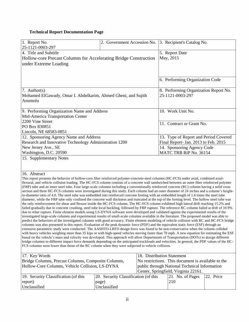
Technical Report Documentation Page

1. Report No. 2. Government Accession No. 3. Recipient's Catalog No.

25-1121-0003-297

4. Title and Subtitle

Hollow-core Precast Columns for Accelerating Bridge Construction

under Extreme Loading

5. Report Date

May, 2015

6. Performing Organization Code

7. Author(s)

Mohamed ElGawady, Omar I. Abdelkarim, Ahmed Gheni, and Sujith

Anumolu

8. Performing Organization Report No.

25-1121-0003-297

9. Performing Organization Name and Address 10. Work Unit No.

Mid-America Transportation Center

2200 Vine Street

PO Box 830851

Lincoln, NE 68583-0851

11. Contract or Grant No.

12. Sponsoring Agency Name and Address 13. Type of Report and Period Covered

Research and Innovative Technology Administration 1200

New Jersey Ave., SE

Washington, D.C. 20590

Final Report- Jan. 2013 to Feb. 2015

14. Sponsoring Agency Code

MATC TRB RiP No. 36154

15. Supplementary Notes

16. Abstract This report presents the behavior of hollow-core fiber reinforced polymer-concrete-steel columns (HC-FCS) under axial, combined axial-

flexural, and vehicle collision loading. The HC-FCS column consists of a concrete wall sandwiched between an outer fiber reinforced polymer

(FRP) tube and an inner steel tube. Four large-scale columns including a conventionally reinforced concrete (RC) column having a solid cross

section and three HC-FCS columns were investigated during this study. Each column had an outer diameter of 24 inches and a column’s height-

to-diameter ratio of 4.0. The steel tube was embedded into reinforced concrete footing with an embedded length of 1.6 times the steel tube

diameter, while the FRP tube only confined the concrete wall thickness and truncated at the top of the footing level. The hollow steel tube was

the only reinforcement for shear and flexure inside the HC-FCS column. The HC-FCS column exhibited high lateral drift reaching 15.2% and

failed gradually due to concrete crushing, steel tube local buckling, followed by FRP rupture. The reference RC-column failed at drift of 10.9%

due to rebar rupture. Finite element models using LS-DYNA software were developed and validated against the experimental results of the

investigated large-scale columns and experimental results of small-scale columns available in the literature. The proposed model was able to

predict the behaviors of the investigated columns with good accuracy. Finite element modeling of vehicle collision with RC and HC-FCS bridge

columns was also presented in this report. Evaluation of the peak dynamic force (PDF) and the equivalent static force (ESF) through an

extensive parametric study were conducted. The AASHTO-LRFD design force was found to be non-conservative when the column collided

with heavy vehicles weighing more than 35 kips or with high-speed vehicles moving faster than 70 mph. A new equation for estimating the ESF

based on the vehicle’s mass and velocity was developed. This approach will allow Departments of Transportation (DOTs) to design different

bridge columns to different impact force demands depending on the anticipated truckloads and velocities. In general, the PDF values of the HC-

FCS columns were lower than those of the RC column when they were subjected to vehicle collision.

17. Key Words 18. Distribution Statement

Bridge Columns, Precast Columns, Composite Columns,

Hollow-Core Columns, Vehicle Collision, LS-DYNA

No restrictions. This document is available to the

public through National Technical Information

Center, Springfield, Virginia 22161.

19. Security Classification (of this

report)

20. Security Classification (of this

page)

21. No. of Pages

210

22. Price

Unclassified Unclassified

iii

Table of Contents

Chapter 1 Literature Review ............................................................................................................ 3 1.1 Concrete-Filled Tube Columns .......................................................................................... 3

1.2 Hollow-Core Columns ....................................................................................................... 4 1.3 Impact Analysis of Vehicle Collision ................................................................................ 9 1.4 Classification of Impact ................................................................................................... 12 1.5 FRP Application in Aerospace Engineering versus Civil Engineering ........................... 13 1.6 Durability of Material Components ................................................................................. 15

1.6.1 Matrix ................................................................................................................................ 15 1.6.2 Fiber ................................................................................................................................... 16 1.6.3 Fiber/Matrix Interface ........................................................................................................ 18

1.7 Various Environmental Exposures on FRP Composite ................................................... 18 1.7.1 Moisture ............................................................................................................................. 18 1.7.2 High Temperatures ............................................................................................................ 20 1.7.3 Low Temperatures ............................................................................................................. 21 1.7.4 Ultraviolet (UV) Light ....................................................................................................... 21

1.8 Accelerated Conditioning and Prediction Methodology.................................................. 22 1.9 Durability of Concrete-Filled FRP Tube (CFFT) Cylinders............................................ 24

Chapter 2 Small Scale HC-FCS Columns under Static Cyclic Axial Loading .......................... 28 2.1 Test Specimens ................................................................................................................ 28

2.2 Material Properties ........................................................................................................... 29 2.3 Experimental set-up and instrumentation ........................................................................ 33

2.4 Loading Schemes ............................................................................................................. 33 2.5 Results and Discussions of Compression Tests ............................................................... 34

2.5.1 General Behavior ............................................................................................................... 34 2.5.2 FRP Axial-Hoop Strains Relation...................................................................................... 37 2.5.3 Local Buckling of the Steel Tubes ..................................................................................... 38

Chapter 3 Large Scale HC-FCS Columns under Axial-Flexural Loading ................................. 41 3.1 Test Specimens ................................................................................................................ 41

3.2 Bill of Quantities-per-Foot ............................................................................................... 45 3.2 Construction Sequence in the Field ................................................................................. 46

3.3 Construction Sequence of the Investigated Columns ...................................................... 48

3.4 Instrumentations ............................................................................................................... 52 3.4.1 Measuring Displacement and Curvature of the Column .................................................... 52 3.4.2 Measuring Strains on the Longitudinal Rebar of the RC-Column..................................... 53 3.4.3 Measuring Strains on the FRP Tubes ................................................................................ 54 3.4.4 Measuring Strains on the Concrete Shell of the HC-FCS Columns .................................. 54 3.4.5 Measuring Strains on the Steel Tubes ................................................................................ 55 3.4.6 Monitoring the Steel Tube Buckling and Sliding Using Webcams ................................... 56

3.6 Loading Protocol and Test Setup ..................................................................................... 56

3.7 Results and Discussion .................................................................................................... 58

Chapter 4 Flexural and Shear Strengths of HC-FCS Columns .................................................. 67 4.1 Flexural Guidelines .......................................................................................................... 67 4.2 Shear Guidelines .............................................................................................................. 73

Chapter 5 Finite Element Modeling ............................................................................................... 75

iv

5.1 Model Description ........................................................................................................... 76 5.1.1 Geometry ........................................................................................................................... 76 5.1.2 Material Models ................................................................................................................. 78 5.1.3 Boundary Conditions and Loading .................................................................................... 80

5.2 Results and Discussions ................................................................................................... 80

5.3 Parametric Study .............................................................................................................. 89 5.3.1 Effects of Axial Load Level on the Behavior of HC-FCS ................................................. 91 5.3.2 Effects of Concrete Wall Thickness on the Behavior of HC-FCS ..................................... 96 5.3.3 Effects of Column Concrete Strength (𝑓𝑐′) on the Behavior of HC-FCS ......................... 97 5.3.4 Effects of D/t Ratio of the Steel Tube on the Behavior of HC-FCS .................................. 98 5.3.5 Effects of the Number of FRP Layers on the Behavior of HC-FCS .................................. 99 5.3.6 Effects of the Number of FRP Layers Combined with D/t Ratio .................................... 101

Chapter 6 Analysis of Vehicle Collision with Reinforced Concrete Bridge Columns ............. 102 6.1 Research Significance .................................................................................................... 102 6.2 Verifying the Finite Element Modeling of a Vehicle Colliding with a Bridge Pier ...... 102

6.3 Modeling the Parametric Study ..................................................................................... 108 6.3.1 Geometry ......................................................................................................................... 109 6.3.2 Columns’ FE Modeling ................................................................................................... 110 6.3.3 Material Models ............................................................................................................... 112 6.3.4 Steel Reinforcement ......................................................................................................... 113 6.3.5 Vehicles FE Models ......................................................................................................... 114

6.4 Results and Discussion of the Parametric Study............................................................ 115 6.4.1 Performance Levels ......................................................................................................... 115 6.4.2 General Comparisons ....................................................................................................... 116 6.4.3 Concrete Material Models ............................................................................................... 120 6.4.4 Unconfined Compressive Strength (𝑓𝑐′) ......................................................................... 124 6.4.5 Strain Rate Effect ............................................................................................................. 125 6.4.6 Percentage of Longitudinal Reinforcement ..................................................................... 125 6.4.7 Hoop Reinforcement ........................................................................................................ 125 6.4.8 Column Span-to-Depth Ratio .......................................................................................... 126 6.4.9 Column Diameter ............................................................................................................. 126 6.4.10 Top Boundary Conditions .............................................................................................. 127 6.4.11 Axial Load Level ........................................................................................................... 129 6.4.12 Vehicle Velocity ............................................................................................................ 129 6.4.13 Vehicle Mass ................................................................................................................. 130 6.4.14 Clear Zone Distance ...................................................................................................... 130 6.4.15 Soil Depth above the Top of the Column Footing ......................................................... 131

6.5 Proposed Variable ESF for Adoption by AASHTO-LRFD .......................................... 133 6.6 Proposed Simplified ESF for Adoption by Eurocode .................................................... 135

Chapter 7 Analysis of Vehicle Collision with HC-FCS Bridge Columns ................................. 138 7.1 Research Significance .................................................................................................... 138 7.2 Parametric Study ............................................................................................................ 138 7.3 FE Modelling of HC-FCSs ............................................................................................ 138 7.4 FE Modeling of Vehicles ............................................................................................... 141 7.5 Results and Discussion of the Parametric Study............................................................ 142

7.5.1 General Comparisons ....................................................................................................... 142 7.5.2 Vehicle Velocity .............................................................................................................. 142 7.5.3 Vehicle Mass ................................................................................................................... 143 7.5.4 Unconfined Compressive Strength (𝑓𝑐′) ......................................................................... 143

v

7.5.5 Strain Rate Effect ............................................................................................................. 143 Chapter 8 Comparisons between RC and HC-FCS Bridge Columns under Vehicle Collision

………………………………………………………………………………………………..145 Chapter 9 Conclusions and Future Work ................................................................................... 148

9.1 Conclusions .................................................................................................................... 148 9.2 Future Work ................................................................................................................... 153

References ....................................................................................................................................... 155

Appendix A: Summary of Columns Results................................................................................ 165 A.1 F4-24-RC Column......................................................................................................... 165

A.1.1 Force-Curvature Relations .............................................................................................. 165 A.1.2 Lateral Drift-Steel Strain Relations ................................................................................ 166

A.2 F4-24-E324 column ...................................................................................................... 168 A.2.1 Force-Curvature Relations .............................................................................................. 168 A.2.2 Lateral Drift-Steel Strain Relations ................................................................................ 169 A.2.3 Lateral drift-FRP strain relations .................................................................................... 178

A.3 F4-24-P124 column....................................................................................................... 183 A.3.1 Force-Curvature Relations .............................................................................................. 183 A.3.2 Lateral Drift-Steel Strain Relations ................................................................................ 184 A.3.3 Lateral Drift-FRP Strain Relations ................................................................................. 191

A.4 F4-24-E344 column ...................................................................................................... 197 A.4.1 Force-Curvature relations ............................................................................................... 197 A.4.2 Lateral Drift-Steel Strain Relations ................................................................................ 198 A.4.3 Lateral Drift-FRP Strain Relations ................................................................................. 205

vi

List of Figures

Figure 1.1 Cross-section of the hollow-core concrete column with two layers of reinforcement

(Mander et al. 1983) ............................................................................................................................. 5

Figure 1.2 Load-displacement relationship of the hollow-core concrete column with two layers of

reinforcement (Mander et al. 1983) ..................................................................................................... 5 Figure 1.3 Cross-section of the hollow-core concrete column with one layer of reinforcement

(Hoshikuma and Priestley 2000) .......................................................................................................... 6 Figure 1.4 Load-displacement relationship of the hollow-core concrete column with one layer of

reinforcement (Hoshikuma and Priestley 2000) .................................................................................. 7 Figure 1.5 Moment-lateral drift relationship of HC-FCS column (Ozbakkaloglu and Idris 2014) ..... 8

Figure 1.6 Axial strain-axial stress relationship of HC-FCS column (Albitar et al. 2013) ................. 9 Figure 1.7 Truck-tractor-trailer accident–FM 1401 Bridge, Texas, 2008 (Buth 2010) ..................... 10 Figure 1.8 Trains accident-overpass outside of Scott City, Missouri, 2013 (McGrath 2013) ........... 10 Figure 2.1 Ready for concrete pouring of HC-FCSs and CFFTs ...................................................... 28

Figure 2.2 (a) steel coupon during tensile test; (b) steel tube A during compression test; (c) failure

modes of the steel tubes A, B, and C ................................................................................................. 31

Figure 2.3 Axial strain-stress curve for steel coupon tensile test...................................................... 31 Figure 2.4 (a) Longitudinal FRP coupon; (b) radial FRP coupon .................................................... 32 Figure 2.5 Strain-stress curve for FRP radial coupon ....................................................................... 33

Figure 2.6 Cyclic loading scheme ..................................................................................................... 34 Figure 2.7 Axial strain-normalized axial load and hoop strain-normalized axial load relations for

groups 1 to 4: (a) and (b) group 1, (c) and (d) group 2, (e) group 3, and (f) group 4 ........................ 35

Figure 2.8 (a) Group 1 failed specimen, (b) Group 2 failed specimen (c) Steel tube local buckling,

(d) Group 3 failed specimen .............................................................................................................. 37 Figure 2.9 Axial load-strain curve of DS-GIII45-32 ........................................................................ 38

Figure 2.10 Actual steel diameter-thickness ratios relative to the AISC manual value versus

increase in capacity ............................................................................................................................ 39 Figure 3.1 Reinforcement details of the investigated columns: (a) F4-24-RC column, (b) F4-24-

E324 column, (c) F4-24-P124 column, and (d) F4-24-E344 column ................................................ 43 Figure 3.2 Construction of HC-FCS column: option “1” .................................................................. 47

Figure 3.3 Construction of HC-FCS column: option “2” .................................................................. 47 Figure 3.4 Preparing reinforcement cages: (a) footing, (b) RC-column ............................................ 48

Figure 3.5 Install reinforcement cages into formwork: (a) footing, (b) RC-column ......................... 48

Figure 3.6 Install the steel tube into the footing: (a) moving the steel tube, (b) putting the steel tube

into the footing, (c) and verticality check of the steel tube ................................................................ 49 Figure 3.7 Concrete pouring of the footing ....................................................................................... 49 Figure 3.8 Install the formwork of the RC-column and the FRP tube for the HC-FCS column ....... 50 Figure 3.9 Concrete pouring of the columns ..................................................................................... 50 Figure 3.10 Install the formwork of the columns’ heads ................................................................... 51

Figure 3.11 Install the reinforcement cage of the column head and concrete pouring ...................... 51 Figure 3.12 Paint the concrete surfaces ............................................................................................. 52 Figure 3.13 Layout of the LVDTs and SPs ........................................................................................ 53 Figure 3.14 Installed strain gauges on two longitudinal rebars of the RC-column ........................... 53 Figure 3.15 Installed strain gauges on FRP tubes ............................................................................. 54

Figure 3.16 Installed vibrating wire strain gauges in the concrete wall thickness ............................ 54

vii

Figure 3.17 Installed strain gauges inside steel tubes: (a) arrangement in cross-section, (b)

arrangement along the height, (c) inserting strain gauges into steel tube, and (d) final view ........... 55 Figure 3.18 Installed webcams inside the steel tubes ....................................................................... 56 Figure 3.19 Column test setup: (a) elevation, (b) sideview .............................................................. 57

Figure 3.20 Lateral displacement loading regime ............................................................................. 57 Figure 3.21 Moment-lateral drift relation: (a) F4-24-RC column, (b) F4-24-E324 column, (c) F4-

24-P124 column, and (d) F4-24-E344 column .................................................................................. 59 Figure 3.22 Columns’ failure: (a) F4-24-RC at 11.5% lateral drift, (b) F4-24-E324 at 15.2% lateral

drift, (c) F4-24-RC damage area, (d) F4-24-E324 FRP rupture, (e) F4-24-P124 FRP rupture, (f) F4-

24-E344 column’s footing damage due to steel tube pullout ............................................................ 62 Figure 3.23 Curvature along the height: (a) F4-24-RC column, (b) F4-24-E324 column, (c) F4-24-

P124 column, and (d) F4-24-E344 column........................................................................................ 63 Figure 3.24 Force-curvature relation at the level of 3.2% of the column’s height: (a) F4-24-RC

column, (b) F4-24-E324 column, (c) F4-24-P124 column, and (d) F4-24-E344 column ................. 64 Figure 3.25 Lateral drift-vertical steel strain relation for: (a) the F4-24-RC column at 4 inch from

the top of the footing, (b) the F4-24-E324 column at 10 inch from the top of the footing, (c) the F4-

24-P124 column at 10 inch from the top of the footing, and (d) the F4-24-E344 column at 10 inch

from the top of the footing ................................................................................................................. 64 Figure 3.26 Lateral drift-hoop steel strain relation for: (a) the F4-24-E324 column at 10 inch from

the top of the footing, (b) the F4-24-P124 column at 10 inch from the top of the footing, and (c) the

F4-24-E344 column at 10 inch from the top of the footing ............................................................... 65 Figure 3.27 Lateral drift-vertical FRP strain relation for: (a) the F4-24-E324 column at 5 inch from


F4-24-E344 column at 5 inch from the top of the footing ................................................................. 65

Figure 3.28 Lateral drift-hoop FRP strain relation for: (a) the F4-24-E324 column at 5 inch from


F4-24-E344 column at 5 inch from the top of the footing ................................................................. 66 Figure 3.29 Lateral drift-concrete strain relation for: (a) the F4-24-P124 column and (b) the F4-24-

E344 column ...................................................................................................................................... 66

Figure 4.1 Cross-sectional analysis.................................................................................................... 71 Figure 4.2 Stress-strain curves of the test columns based on the model of Yu et al. (2006) ............. 72

Figure 5.2 Model components: (a) steel tube, (b) concrete column, (c) FRP tube, (d) concrete

footing, and (e) loading stub .............................................................................................................. 78

Figure 5.3 Experimental hysteretic vs. FE backbone curves and analytical results for the HC-FCS

large scale columns: (a) F4-24-E324 column, (b) F4-24-P124 column, and (c) F4-24-E344 column

............................................................................................................................................................ 83 Figure 5.4 Experimental (Ozbakkaloglu and Idris 2014 ©ASCE) vs. FE backbone curves for

specimens: (a) DST-1, (b) DST-2, (c) DST-3, (d) DST-5, (e) DST-6, (f) DST-7, and (g) DST-9 ... 84 Figure 5.5 Moving of neutral axis (N.A.) under lateral loading (hatched area is the compression

side) .................................................................................................................................................... 85

Figure 5.6 Maximum confined concrete stress of the column DST-1 in GPa. (1 GPa = 145 ksi).... 85 Figure 5.7 FE vs. experimental (Ozbakkaloglu and Idris 2014 ©ASCE) strain profile of the FRP

tube of column DST-1 ....................................................................................................................... 86 Figure 5.8 Fiber rupture of FRP tube of the column DST-7: (a) FE result and (b) experimental

result (Ozbakkaloglu and Idris 2014 ©ASCE) .................................................................................. 89

viii

Figure 5.9 Lateral drift vs. moment for finite element parametric study: (a) load level change, (b)

concrete wall thickness change, (c) concrete strength change, (d) D/t for steel tube change, (e)

number of FRP layers change ............................................................................................................ 92 Figure 5.10 Percent change of the bending strength and the maximum lateral drift versus; (a)

loading level, (b) concrete wall thickness, (c) concrete strength, (d) D/t for steel tube, (e) number of

FRP layers, (f) number of FRP layers with different steel tube D/t .................................................. 93 Figure 5.11 Column-footing connection: (a) closed connection, and (b) uplift of the heel of the

connection .......................................................................................................................................... 96 Figure 6.1 3D- view of the FE model for verification against El-Tawil’s et al. (2005) results ...... 104

Figure 6.2 Components of the FE model for verification against El-Tawil’s et al. results (2005) . 106 Figure 6.3 The reduced FE model of Chevrolet pickup: (a) 3D-view, and (b) side view of the

collision event of the reduced FE model of Chevrolet pickup with bridge pier (velocity = 69 mph

and time = 0.05 second) ................................................................................................................... 107 Figure 6.4 FE results from current study versus those from El-Tawil et al. (2005) FE results; (a)

vehicle velocity of 34 mph, (b) vehicle velocity of 69 mph, (c) vehicle velocity of 84 mph, and (d)

PDF and ESF versus the vehicle velocities...................................................................................... 107 Figure 6.5 F.E. model of the bridge pier “C0” for the parametric study; (a) 3D-view, and (b)

detailed side view of the pier components ....................................................................................... 110 Figure 6.6 3D-view of the FE model: (a) the Ford single unit truck, (b) Chevrolet pickup detailed

model................................................................................................................................................ 115

Figure 6.7 (a) Performance levels of the examined columns according to the results of FE, (b)

normalized forces to the ESF of AASHTO-LRFD (600 kips), and (c) damage ratio of the dynamic

and static forces for the examined columns ..................................................................................... 117

Figure 6.8 Effects of various concrete material models: (a) time-impact force, (b) PDF vs. ESF vs.

AASHTO-LRFD, (c) time-total kinetic energy, and (d) time-vehicle displacement ...................... 123 Figure 6.9 Time-energies relations of the FE model C0 ................................................................. 124

Figure 6.10 Effects of (a) 𝑓𝑐′, (b) strain rate, (c) longitudinal reinforcements ratio, (d) hoop

reinforcements ratio, (e) span-to-depth ratio, and (f) column diameters on PDF and ESF ............. 128

Figure 6.11 Buckling of rebars of column C14 having a diameter of 4 ft scaled 50 times ............ 129 Figure 6.12 Effects of (a) top boundary conditions, (b) axial load level, (c) vehicle velocities, (d)

vehicle masses, (e) clear zone distance, and (f) soil depth above the top of column footing on PDF

and ESF ............................................................................................................................................ 132 Figure 6.13 Kinetic energy-ESF relation for the proposed equation of KEBESF and the FE results

.......................................................................................................................................................... 135

Figure 6.14 Momentum-normalized ESF relation for the proposed equation of MBESF and the FE

results ............................................................................................................................................... 136 Figure 6.15 Normalized forces of KEBESF and MBESF versus the normalized shear capacity and the

ESF of AASHTO-LRFD.................................................................................................................. 137 Figure 7.1 FE model of the bridge pier “C0” for the parametric study: (a) detailed side view of the

pier components, (b) 3D-view, (c) FE model of the Ford single unit truck, (d) FE detailed model of

the Chevrolet pickup ........................................................................................................................ 141 Figure 7.2 Vehicle collision with the HC-FCS column .................................................................. 142

Figure 7.3 Effects of (a) vehicle velocity, (b) vehicle mass, (c) fc′, and (d) strain rate on PDF and

ESF ................................................................................................................................................... 144 Figure 8.1 Time vs impact force for HC-FCS column and RC column under vehicle collision with

a velocity of: (a) 70 mph, (b) 50 mph, and (c) 20 mph .................................................................... 146

ix

Figure 8.2 Column strain contour: (a) RC column and (b) HC-FCS column ................................. 147 Figure 11.1 Force-curvature relation of the F4-24-RC column: (a) at level of 3.2% of the column’s

height, (b) at level of 8.4% of the column’s height, (c) at level of 13.7% of the column’s height, and

(d) at level of 21.6% of the column’s height ................................................................................... 165

Figure 11.2 Lateral drift-steel rebar microstrain relation in the north direction .............................. 166 Figure 11.3 Lateral drift-steel rebar microstrain relation in the north direction .............................. 167 Figure 11.4 Force-curvature relation the F4-24-E324 column: (a) at level of 3.2% of the column’s


(d) at level of 21.6% of the column’s height ................................................................................... 168

Figure 11.5 Lateral drift-steel tube microstrain relation at 20 inch above the top of the footing .... 169 Figure 11.6 Lateral drift-steel tube microstrain relation at 15 inch above the top of the footing .... 170

Figure A.7 Lateral drift-steel tube microstrain relation at 10 inch above the top of the footing ..... 171 Figure A.8 Lateral drift-steel tube microstrain relation at 5 inches above the top of the footing .... 172 Figure A.9 Lateral drift-steel tube microstrain relation at the level of the top of the footing ......... 173 Figure A.10 Lateral drift-steel tube microstrain relation at 5 inch below the top of the footing ..... 174

Figure A.11 Lateral drift-steel tube microstrain relation at 10 inch below the top of the footing ... 175 Figure A.12 Lateral drift-steel tube microstrain relation at 15 inch below the top of the footing ... 176

Figure A.13 Lateral drift-steel tube microstrain relation at 20 inch below the top of the footing ... 177 Figure A.14 Lateral drift- FRP tube microstrain relation at 25 inch above the top of the footing .. 178 Figure A.15 Lateral drift- FRP tube microstrain relation at 20 inch above the top of the footing .. 179

Figure A.16 Lateral drift- FRP tube microstrain relation at 15 inch above the top of the footing .. 180 Figure A.17 Lateral drift- FRP tube microstrain relation at 10 inch above the top of the footing .. 181

Figure 11.18 Lateral drift-FRP tube microstrain relation at 5 inch above the top of the footing .... 182

Figure A.19 Force-curvature relation of the F4-24-P124 column: (a) at level of 3.2% of the

column’s height, (b) at level of 8.4% of the column’s height, (c) at level of 13.7% of the column’s

height, and (d) at level of 21.6% of the column’s height ................................................................. 183

Figure A.20 Lateral drift-steel tube microstrain relation at 20 inch above the top of the footing .. 184 Figure A.21 Lateral drift-steel tube microstrain relation at 15 inch above the top of the footing ... 185 Figure A.22 Lateral drift-steel tube microstrain relation at 10 inch above the top of the footing ... 186

Figure A.23 Lateral drift-steel tube microstrain relation at 5 inch above the top of the footing ..... 187 Figure A.24 Lateral drift-steel tube microstrain relation at the level of the top of the footing ....... 188

Figure A.25 Lateral drift-steel tube microstrain relation at 5 inch below the top of the footing ..... 189 Figure A.26 Lateral drift-steel tube microstrain relation at 10 inch below the top of the footing ... 190

Figure A.27 Lateral drift-FRP tube microstrain relation at 25 inch above the top of the footing ... 191

Figure A.28 Lateral drift-FRP tube microstrain relation at 20 inch above the top of the footing ... 192

Figure A.29 Lateral drift- FRP tube microstrain relation at 15 inch above the top of the footing .. 193 Figure A.30 Lateral drift- FRP tube microstrain relation at 10 inch above the top of the footing .. 194 Figure A.31 Lateral drift- FRP tube microstrain relation at 5 inch above the top of the footing .... 195 Figure A.32 Lateral drift- FRP tube microstrain relation at the top of the footing.......................... 196 Figure A.33 Force-curvature relation of the F4-24-P124 column: (a) at level of 3.2% of the


height, and (d) at level of 21.6% of the column’s height ................................................................. 197 Figure A.34 Lateral drift-steel tube microstrain relation at 20 inch above the top of the footing ... 198 Figure A.35 Lateral drift-steel tube microstrain relation at 15 inch above the top of the footing ... 199 Figure A.36 Lateral drift-steel tube microstrain relation at 10 inch above the top of the footing ... 200

Figure A.37 Lateral drift-steel tube microstrain relation at 5 inch above the top of the footing ..... 201

x

Figure A.38 Lateral drift-steel tube microstrain relation at the level of the top of the footing ....... 202 Figure A.39 Lateral drift-steel tube microstrain relation at 5 inch below the top of the footing ..... 203 Figure A.40 Lateral drift-steel tube microstrain relation at 10 inch below the top of the footing ... 204 Figure A.41 Lateral drift-FRP tube microstrain relation at 25 inch above the top of the footing ... 205

Figure A.42 Lateral drift-FRP tube microstrain relation at 20 inch above the top of the footing ... 206 Figure A.43 Lateral drift- FRP tube microstrain relation at 15 inch above the top of the footing .. 207 Figure A.44 Lateral drift- FRP tube microstrain relation at 10 inch above the top of the footing .. 208 Figure A.45 Lateral drift- FRP tube microstrain relation at 5 inch above the top of the footing .... 209 Figure A.46 Lateral drift- FRP tube microstrain relation at the top of the footing.......................... 210

xi

List of Tables

Table 1.1 Environmental reduction factor for various FRP systems and exposure conditions ........ 27 Table 2.1 Specimens descriptions ...................................................................................................... 29

Table 2.2 Concrete mixture proportions ............................................................................................ 29 Table 2.3 Properties of steel tubes .................................................................................................... 32 Table 2.4 Properties of saturated FRP according to manufacturer’s data ......................................... 32 Table 2.5 Properties of the prefabricated GFRP tubes ...................................................................... 32 Table 2.6 Steel tube D/t ratio of HC-FCS columns of literature and of our work ............................ 40

Table 3.1 Summary of the columns’ variables .................................................................................. 44 Table 3.2 Concrete mixture proportions ........................................................................................... 44

Table 3.3 Summary of the unconfined concrete strength of the columns and the footings .............. 44 Table 3.4 Steel properties of the rebars and steel tubes .................................................................... 44 Table 3.5 FRP tubes properties ......................................................................................................... 45 Table 3.6 Summary of bill of quantities-per-foot of F4-24-RC and F4-24-P124 columns .............. 46

Table 3.7 Summary of the columns’ results ...................................................................................... 63 Table 4.1 Summary of the tested large scale columns’ results versus simplified analytical method 72

Table 4.2 Summary of Ozbakkaloglu and Idris (2014) experimental results versus simplified

analytical method ............................................................................................................................... 73 Table 5.1 Summary of columns variables (reproduced after Ozbakkaloglu and Idris 2014) ........... 75

Table 5.2 Summary of orthotropic material properties for FRP tubes .............................................. 79 Table 5.3 Summary of the tested large scale columns’ results vs. finite element results ................. 82

Table 5.4 Summary of Ozbakkaloglu and Idris (2014) experimental results vs. finite element

results ................................................................................................................................................. 82

Table 5.5 Summary of the parametric study results .......................................................................... 94 Table 5.6 Results summary of number of FRP layers versus steel tube D/t ratios ......................... 100

Table 6.1 Summary of FE results of current study versus El-Tawil et al. (2005) ........................... 108 Table 6.2 Summary of the examined columns’ parameters ............................................................ 111 Table 6.3 Summary of the normalized PDFs, ESFs, and shear capacity of all of the columns and

their performance levels ................................................................................................................... 122 Table 6.4 Summary of the prediction of the different approaches including AASHTO-LRFD ..... 123

Table 8.1 Summary of the examined columns’ variables ................................................................ 146

xii

Acknowledgements

The authors would like to acknowledge the many individuals and organizations that made

this research project possible. The authors wish to extend a very sincere thank you to the Missouri

Department of Transportation (MoDOT). In addition to their financial support, the authors

appreciate MoDOT’s vision and commitment to innovative concepts and pushing the boundaries of

current practice. In particular, the success of this project would not have been possible without the

support, encouragement, and patience of Mr. Andrew Hanks. The authors also wish to extend a

sincere thank you to MoDOT’s Technical Advisory Group for their thorough review of the final

report draft and their many insightful comments, namely Andrew Hanks, Dennis Heckman, and

Gregory Sanders. Special thanks also to Mr. Bill Stone for his flexibility, insight, and continued

support of the project.

The authors would also like to thank the Mid-America Transportation Center (MATC)

which provided valuable match funding from the United States Department of Transportation

through RITA. The authors also extend their appreciation to the National University Transportation

Center (NUTC) at Missouri University of Science and Technology (Missouri S&T).

The authors would also like to thank the companies that provided material contributions necessary

for the successful completion of this project, including Pittsburgh Pipe and Atlas Tube.

Appreciation is extended to Fyfe CO. LLC for partially donating some of the materials used in the

experimental work.

Finally, the authors would like to thank Missouri S&T for their valuable contributions to the

research. The authors also appreciate the tireless staff of the Department of Civil, Architectural and

Environmental Engineering and the Center for Infrastructure Engineering Studies. Their assistance

xiii

both inside and out of the various laboratories was invaluable to the successful completion of this

project.

xiv

Disclaimer

The contents of this report reflect the views of the authors, who are responsible for the facts

and the accuracy of the information presented herein. This document is disseminated under the

sponsorship of the U.S. Department of Transportation’s University Transportation Centers

Program, in the interest of information exchange. The U.S. Government assumes no liability for the

contents or use thereof.

xv

Executive Summary

This study has developed an innovative resilient, durable, and quickly-constructed precast

hollow-core fiber reinforced polymer-concrete-steel (HC-FCS) bridge column. The cross-section of

the HC-FCS column consists of a concrete shell sandwiched between an inner steel tube and an

outer fiber reinforced polymer (FRP) tube. The inner steel tube was embedded into the concrete

footing while the outer FRP was discontinued at the footing top surface level, i.e., the FRP tube

provides confinement and stay-in-place formwork only. Hence, the system ductility is mainly

attributed to the steel tube and high-confinement of the concrete shell. The HC-FCS column has the

following several distinct advantages over columns constructed out of reinforced concrete (RC).

The HC-FCS column uses 60 to 75% less concrete material since it has a hollow-core. The HC-

FCS column, also, requires reduced freight cost when implemented with precast construction. The

inner steel and outer FRP tubes provide a continuous confinement for the concrete shell; hence, the

concrete shell achieves significantly higher strain, strength, and ductility compared to unconfined

concrete. The HC-FCS represents a compact engineering system; the steel and FRP tubes together

act as stay-in-place formworks. The steel tube acts as flexural and shear reinforcement. The

concrete shell will delay the local buckling of the steel tube and hence make more efficient use of

the steel tube. The HC-FCS column has high corrosion resistance since the steel tube is well

protected by the corrosion-free outer FRP tube and concrete core. The report focuses on

investigating the behavior of HC-FCS columns under combined axial-flexural loads. Moreover, the

behavior of the column under vehicle impact was investigated as well. Finally, design guidelines

were developed. The behavior of the HC-FCS columns under different extreme load conditions

were compared to those of conventional concrete having solid cross section. The report also

xvi

introduces, for the first time, a design equation to predict the equivalent static impact force of

vehicle collision with bridge columns that can be implemented in AASHTO-LRFD.

The report includes eleven chapters. Chapter 1 introduces a literature review on the FRP and

its applications, behavior of hollow-core columns, and vehicle collision with bridge columns.

Chapter 2 explains the behavior of the HC-FCS columns under axial loading. Chapter 3 details the

construction, detailing, testing protocol, and results of four large-scale columns under constant axial

load and static cyclic lateral loads. Chapter 4 contains the flexural and shear strength guidelines of

the HC-FCS columns. Chapter 5 presents finite element analysis of the HC-FCS columns and an

extensive parametric study to clarify the behavior under lateral loading. Chapter 6 explains the

vehicle collision with RC columns through an extensive parametric study to clarify the behavior.

Chapter 7 investigates the vehicle collision with HC-FCS columns through a parametric study to

clarify the behavior. Chapter 8 presents the comparison between the behavior of RC and HC-FCS

columns under vehicle collision. Chapter 9 contains conclusions and recommendations for future

work. Finally, Appendix A contains a summary of the results of large-scale columns.

Based on the results of this study, the research team recommends the HC-FCS columns for

bridge construction. However, to facilitate this implementation, additional work is required in order

to tailor the steel and FRP tubes as well as to develop construction details for column/girder

connection. Further work is also required to address the shear, torsion, and development length of

the inner steel tube. Finally, the behavior of the HC-FCS column having a thin steel tube also needs

further investigation.

3

Chapter 1 Literature Review

1.1 Concrete-Filled Tube Columns

A significant amount of research was recently devoted to developing accelerated bridge

construction (ABC) systems. These ABC systems offer several benefits, including reduced

construction time, minimal traffic disruptions, reduced life-cycle costs, improved construction

quality, and improved safety (Dawood et al. 2012). Concrete-filled steel tubes (CFSTs) are widely

used as bridge columns in Japan, China, and Europe to not only accelerate construction but also to

obtain superior seismic performance. In the US, CFSTs are used as piles and bridge piers.

However, their application is limited, primarily, as a result of inconsistent design code provisions

(Moon et al. 2013). Incorporated CFST members have several advantages over either steel or

reinforced concrete (RC) members. The steel tubes act as a stay-in-place formwork, flexural and

shear reinforcement, and a confinement to the inside concrete core, increasing the member’s

ductility and strength. The tubes prevent concrete spalling so that the concrete core continues to

function as a bracing for the steel tube. Therefore, the concrete core delays both local and global

buckling under compression loads (Hajjar 2000).

The CFST members dissipate more energy than those made from either traditional steel or

RC members. On a strength-per-dollar basis, CFST members are cheaper than traditional steel

members; they are comparable in price to traditional RC members. A concrete core can be

reinforced with steel rebar to further improve the member’s performance while facilitating

connections to other members. Limited performance data is available, however, for steel rebar

reinforced CFST columns (Moon et al. 2013; Hajjar 2000).

FRP tubes have gained acceptance as an alternative to steel tubes in CFSTs. Concrete-filled

fiber tubes (CFFT) have benefits that are similar to those of CFSTs. However, unlike steel tubes,

4

FRP tubes have a lighter weight-to-strength ratio and a higher corrosion resistance than steel tubes.

Several researchers investigated the seismic behavior of CFFT columns (Zhu et al. 2006). Shin and

Andrawes (2010) investigated the behavior of CFFTs that were confined by a shape memory alloy.

ElGawady et al. (2010) and ElGawady and Sha’lan (2011) conducted static cyclic tests on both

segmental precast post-tensioned CFFT columns and two-column bents. Upon conducting finite

element analysis, ElGawady and Dawood (2012) and Dawood and ElGawady (2013) developed a

design procedure for precast post-tensioned CFFTs.

1.2 Hollow-Core Columns

Hollow-core concrete columns are often used for very tall bridge columns in seismic areas

including California, New Zealand, Japan, Italy, etc. Hollow-core cross-sections reduce the mass of

the column which reduces the bridge self-weight contribution to the inertial mode of vibration

during an earthquake. The hollow-core columns also reduce the foundations dimensions, thereby

reducing the construction costs substantially. These advantages have increased the use of hollow-

core columns instead of similar solid members.

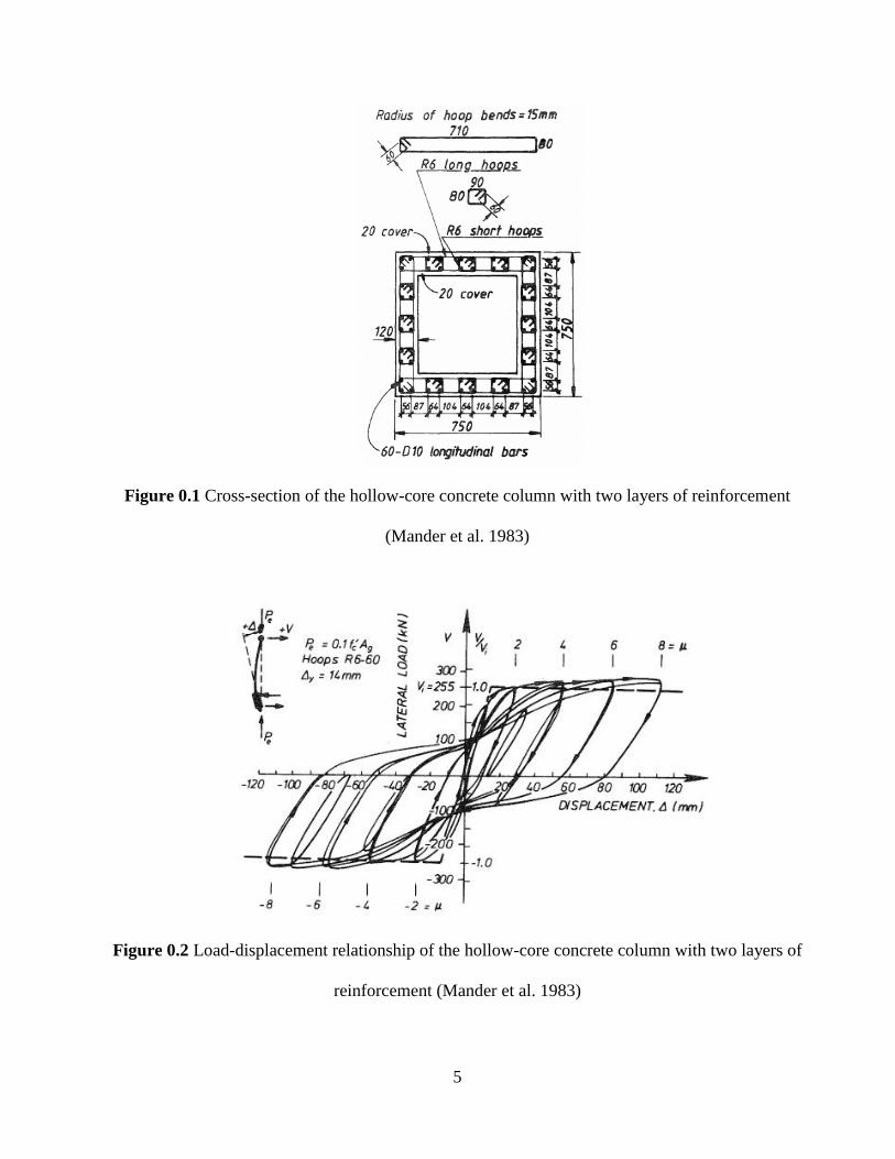
Mander et al. (1983) investigated hollow-core concrete columns that have two layers of

longitudinal and transverse reinforcement placed near in-/outside faces and cross ties placed

throughout the wall’s thickness (fig. 1.1). These columns can exhibit a ductile behavior (fig. 1.2).

However, they increase the labor cost making it not a cost-effective construction option.

5

Figure 0.1 Cross-section of the hollow-core concrete column with two layers of reinforcement

(Mander et al. 1983)

Figure 0.2 Load-displacement relationship of the hollow-core concrete column with two layers of

reinforcement (Mander et al. 1983)

6

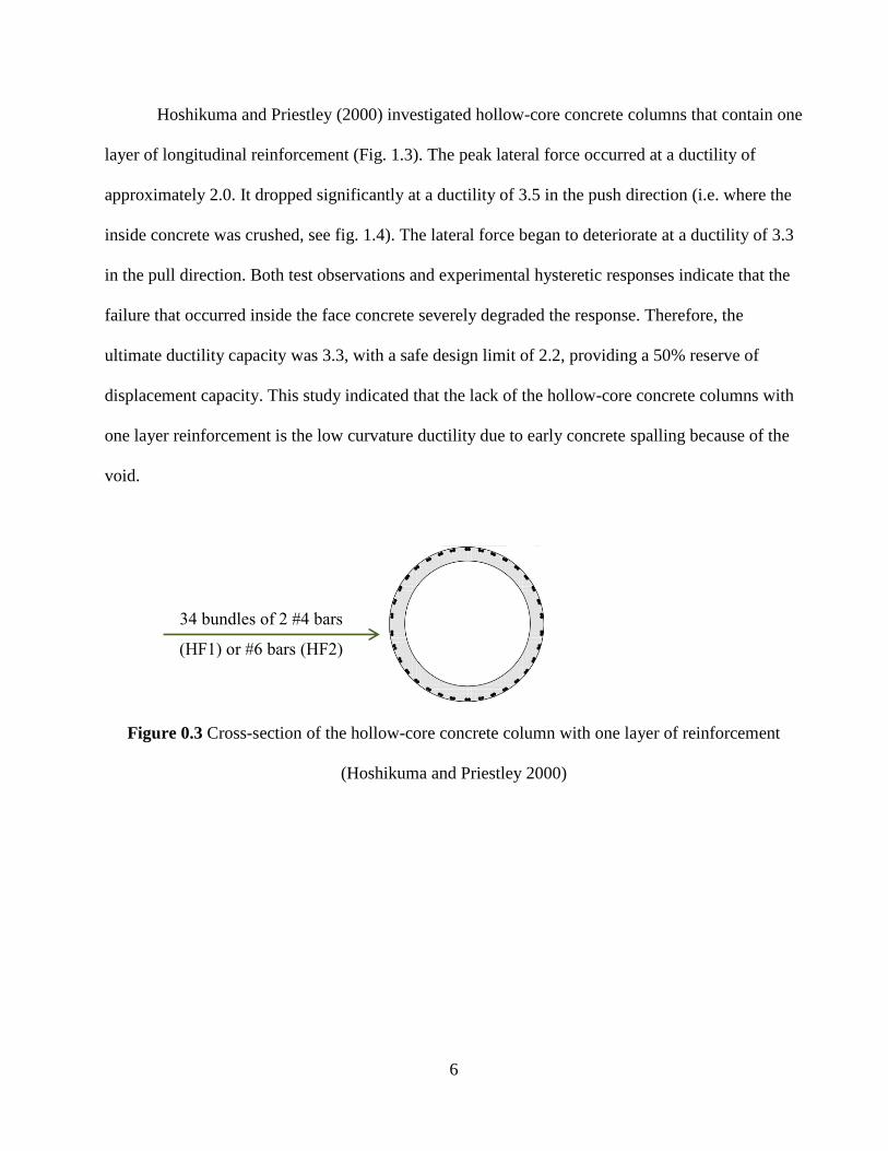
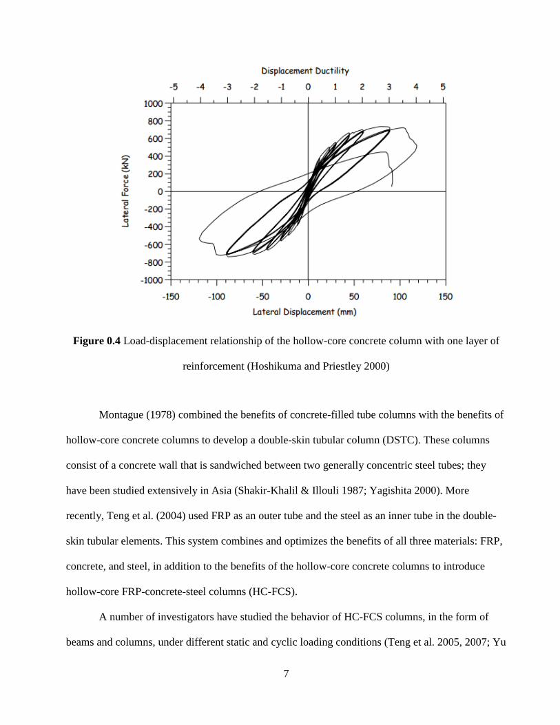
Hoshikuma and Priestley (2000) investigated hollow-core concrete columns that contain one

layer of longitudinal reinforcement (Fig. 1.3). The peak lateral force occurred at a ductility of

approximately 2.0. It dropped significantly at a ductility of 3.5 in the push direction (i.e. where the

inside concrete was crushed, see fig. 1.4). The lateral force began to deteriorate at a ductility of 3.3

in the pull direction. Both test observations and experimental hysteretic responses indicate that the

failure that occurred inside the face concrete severely degraded the response. Therefore, the

ultimate ductility capacity was 3.3, with a safe design limit of 2.2, providing a 50% reserve of

displacement capacity. This study indicated that the lack of the hollow-core concrete columns with

one layer reinforcement is the low curvature ductility due to early concrete spalling because of the

void.

Figure 0.3 Cross-section of the hollow-core concrete column with one layer of reinforcement

(Hoshikuma and Priestley 2000)

34 bundles of 2 #4 bars

(HF1) or #6 bars (HF2)

7

Figure 0.4 Load-displacement relationship of the hollow-core concrete column with one layer of

reinforcement (Hoshikuma and Priestley 2000)

Montague (1978) combined the benefits of concrete-filled tube columns with the benefits of

hollow-core concrete columns to develop a double-skin tubular column (DSTC). These columns

consist of a concrete wall that is sandwiched between two generally concentric steel tubes; they

have been studied extensively in Asia (Shakir-Khalil & Illouli 1987; Yagishita 2000). More

recently, Teng et al. (2004) used FRP as an outer tube and the steel as an inner tube in the double-

skin tubular elements. This system combines and optimizes the benefits of all three materials: FRP,

concrete, and steel, in addition to the benefits of the hollow-core concrete columns to introduce

hollow-core FRP-concrete-steel columns (HC-FCS).

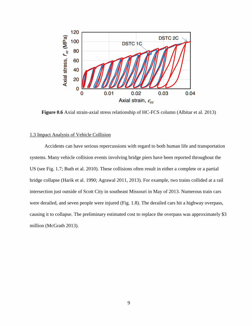
A number of investigators have studied the behavior of HC-FCS columns, in the form of

beams and columns, under different static and cyclic loading conditions (Teng et al. 2005, 2007; Yu

8

et al. 2006, 2010; Wong et al. 2008; Lu et al. 2010; Huang et al. 2013; Abdelkarim and ElGawady

2014a and 2014b; Abdelkarim et al. 2015; Li et al. 2014a; Li et al. 2014b). The results of the

conducted experimental tests under axial compression, flexure, and combined axial compression

and flexure showed high concrete confinement and ductility (e.g., see figs. 1.5 and 1.6).

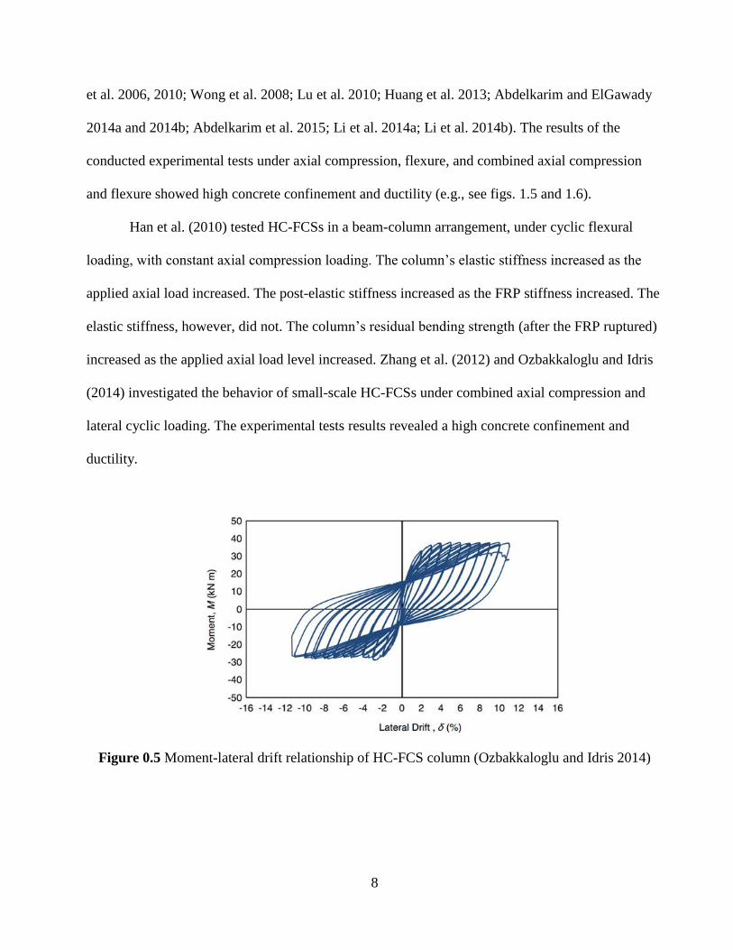
Han et al. (2010) tested HC-FCSs in a beam-column arrangement, under cyclic flexural

loading, with constant axial compression loading. The column’s elastic stiffness increased as the

applied axial load increased. The post-elastic stiffness increased as the FRP stiffness increased. The

elastic stiffness, however, did not. The column’s residual bending strength (after the FRP ruptured)

increased as the applied axial load level increased. Zhang et al. (2012) and Ozbakkaloglu and Idris

(2014) investigated the behavior of small-scale HC-FCSs under combined axial compression and

lateral cyclic loading. The experimental tests results revealed a high concrete confinement and

ductility.

Figure 0.5 Moment-lateral drift relationship of HC-FCS column (Ozbakkaloglu and Idris 2014)

9

Figure 0.6 Axial strain-axial stress relationship of HC-FCS column (Albitar et al. 2013)

1.3 Impact Analysis of Vehicle Collision

Accidents can have serious repercussions with regard to both human life and transportation

systems. Many vehicle collision events involving bridge piers have been reported throughout the

US (see Fig. 1.7; Buth et al. 2010). These collisions often result in either a complete or a partial

bridge collapse (Harik et al. 1990; Agrawal 2011, 2013). For example, two trains collided at a rail

intersection just outside of Scott City in southeast Missouri in May of 2013. Numerous train cars

were derailed, and seven people were injured (Fig. 1.8). The derailed cars hit a highway overpass,

causing it to collapse. The preliminary estimated cost to replace the overpass was approximately $3

million (McGrath 2013).

http://www.ibtimes.com/reporters/jj-mcgrath

10

Figure 0.7 Truck-tractor-trailer accident–FM 1401 Bridge, Texas, 2008 (Buth 2010)

Figure 0.8 Trains accident-overpass outside of Scott City, Missouri, 2013 (McGrath 2013)

Numerous researchers have used LS-DYNA software to investigate the modeling of

concrete columns under extreme loading (Abdelkarim and ElGawady 2015 and 2014b; Sharma et

al. 2012; Fouche and Bruneau 2010; Thilakarathna et al. 2010). El-Tawil et al. (2005) used this

software to examine two bridge piers that had been impacted by different trucks at different

velocities. Both the peak dynamic force (PDF: the maximum contact force of the vehicle collision

on the bridge column) and the equivalent static force (ESF) were evaluated. The American


11

Association of State Highway and Transportation Officials- Load and Resistance Factor Bridge

Design Specifications 5th edition (AASHTO-LRFD 2010) mandates that both abutments and piers

located within a distance of 30 ft from the roadway’s edge must be designed to allow for a ESF of

the collision load of 400 kips. El-Tawil et al. (2005) suggested that the AASHTO-LRFD could be

non-conservative and that the ESF should be higher than 400 kips.

Buth et al. (2011) experimentally studied the collision of tractor-trailers into a rigid column

that was constrained at both ends. Numerical models were used to conduct a parametric study on

single unit trucks (SUTs). The investigated parameters included the pier’s diameter, the vehicle’s

weight, the vehicle’s velocity, and the cargo’s state (rigid vs. deformable). Based on the results

gathered during this study, the ESF of the AASHTO-LRFD was increased to 600 kips and applied

to a bridge pier in a direction of zero to 15 degrees with the edge of the pavement in a horizontal

plane, at a distance of 5.0 ft above ground.

Sharma et al. (2012) used a performance-based response to investigate the effect of a

vehicle’s impact on a reinforced concrete column. They suggested that four different damage levels

and three different performance levels be used to evaluate the column’s response. Agrawal et al.

(2013) investigated the effects of different seismic design details on a pier’s response to vehicle

impact loading. They proposed that a new procedure be used to calculate the ESF; this procedure is

based on the vehicle’s mass and velocity. A proposed equation was used to calculate the PDF. The

ESF was calculated by dividing the calculated PDF by the damage ratio (which is dependent on the

required performance level being 2, 5, and > 5 for minor, moderate, and high damage levels,

respectively). This procedure produced variable values of ESF rather than the constant ESF

recommended by AASHTO-LRFD.

12

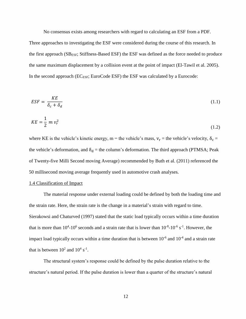
No consensus exists among researchers with regard to calculating an ESF from a PDF.

Three approaches to investigating the ESF were considered during the course of this research. In

the first approach (SBESF; Stiffness-Based ESF) the ESF was defined as the force needed to produce

the same maximum displacement by a collision event at the point of impact (El-Tawil et al. 2005).

In the second approach (ECESF; EuroCode ESF) the ESF was calculated by a Eurocode:

𝐸𝑆𝐹 = 𝐾𝐸

𝛿𝑐 + 𝛿𝑑 (1.1)

𝐾𝐸 =1

2 𝑚 𝑣𝑟

2

(1.2)

where KE is the vehicle’s kinetic energy, m = the vehicle’s mass, vr = the vehicle’s velocity, δc =

the vehicle’s deformation, and δd = the column’s deformation. The third approach (PTMSA; Peak

of Twenty-five Milli Second moving Average) recommended by Buth et al. (2011) referenced the

50 millisecond moving average frequently used in automotive crash analyses.

1.4 Classification of Impact

The material response under external loading could be defined by both the loading time and

the strain rate. Here, the strain rate is the change in a material’s strain with regard to time.

Sierakowsi and Chaturved (1997) stated that the static load typically occurs within a time duration

that is more than 104-106 seconds and a strain rate that is lower than 10-8-10-6 s-1. However, the

impact load typically occurs within a time duration that is between 10-6 and 10-4 and a strain rate

that is between 102 and 104 s-1.

The structural system’s response could be defined by the pulse duration relative to the

structure’s natural period. If the pulse duration is lower than a quarter of the structure’s natural

13

period, the system’s response is impacted. However, if the pulse duration is larger than four times

the structure’s natural period, the system’s response is quasi-static.

In a vehicle collision event with bridge piers, the bridge pier (the body that is struck) is

considered to be the target while the vehicle (the body that impacts the target) is considered to be

the projectile. The collision’s relative degree of softness/hardness classifies the type of impact that

occurs. Therefore, the impact type can be classified by the projectile/target interaction into the

following categories: hard/soft, hard/hard, soft/hard, and soft/soft. This classification significantly

affects the induced dynamic contact force between the projectile and the target. If a soft projectile

interacts with a rigid target, the stress waves propagate within the projectile upon contact, damaging

the projectile. When this interaction occurs, the projectile absorbs most of the impact’s kinetic

energy in the form of plastic deformation. If a hard projectile interacts with a soft target, the stress

waves propagate within the target upon contact. Hence, the target absorbs most of the impact’s

kinetic energy in the form of plastic deformation. Consequently, absorbing the kinetic energy from

the projectile’s mass and velocity is the key parameter when preparing the impact analysis.

1.5 FRP Application in Aerospace Engineering versus Civil Engineering

Fiber-reinforced polymer (FRP) is outstanding in its high strength-to-mass ratio, easy

construction, and high resistance to environmental exposure. It has been used for retrofitting

existing structures and new infrastructure construction in the area of civil engineering during the

past decades. The FRP that is used to retrofit old structures is the FRP wrap in which the fibers are

typically oriented in a circumferential direction. For new construction like concrete filled FRP

cylinders, prefabricated FRP tubes are employed which are typically thicker than FRP cloths and

there’s no overlapping zone. Even though the FRP materials exhibited greater durability to

environmental exposure than conventional materials (i.e., concrete and steel), the rigorous estimate

14

of the resistance of FRP composite structures to severe environmental exposures and their service

life cycles still face uncertainties. This study included a review of technical literatures that

discussed FRP composite’s durability when subjected to various environmental exposures. The

review began with FRP applications in aerospace engineering vs. civil engineering and the reasons

why the durability of FRP used in civil engineering needs to be studied. Next, the durability of each

constitution component (fiber, matrix, and fiber/matrix interface) was presented, followed by the

effects of various environmental exposures on FRP at the composite level. The accelerated aging

methodology and findings for FRP confined concrete cylinders were reviewed at the end.

The first known FRP product was a boat hull manufactured in the mid-1930s as part of a

manufacturing experiment using a fiberglass fabric and polyester resin laid in a foam mold (ACI

2007). The defense industry began to use these FRP composite materials, particularly in aerospace

and naval applications in the early 1940s. The U.S. Air Force and Navy capitalized on FRP

composite’s high strength-weight ratio, noncorrosive, nonmagnetic, and nonconductive

characteristics.

FRP composite products were first used to reinforce concrete structures in the mid-1950s.

Since then, FRP composite applications in civil engineering have evolved from temporary

structures to the restoration of historic buildings. A major development in FRP used for the area of

civil engineering has been the application of externally bonded FRP in rehabilitating and

strengthening concrete structures.

The application of FRP composites in civil engineering, however, is not a direct transfer

from that in aerospace engineering. The FRP materials used in aerospace engineering are far more

advanced than those needed in public infrastructures. Those advanced FRP materials are cured at a

very high temperature and provide excellent quality and properties. The FRP used in aerospace

15

engineering is typically cured above 100°C, producing a higher glass transition temperature in the

resin and more durable joints. At the same time, these FRP materials are quite expensive. On the

other hand, most infrastructures just need cost-effective materials for construction and rehabilitation

purposes. In civil engineering application, resin acting as binders for fibers can be adequately cured

at ambient temperatures and still offer comparable quality. The properties are more desirable and

also practical. This efficient fabrication method helps reduce costs and increase popularity in the

civil market.

The primary obstacle that hinders the wide application of FRP composites in civil

infrastructures is the long-term durability performance, especially when the structure is undergoing

combined harsh environmental conditions. Even though the FRP system has been used in aerospace

engineering for almost a century and demonstrated good durability characteristics, those FRP

possess are of a higher quality than the one currently used in civil infrastructures, and its excellent

durability performance cannot be directly applied to the civil engineering case. This is why many

researchers did a lot of research and study during the past few decades to investigate the durability

of this new material in civil engineering applications.

1.6 Durability of Material Components

1.6.1 Matrix

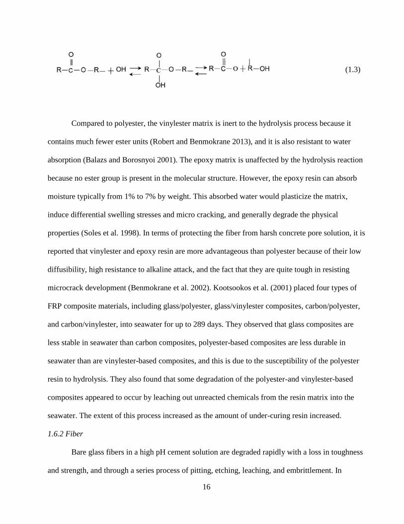
The ester group, which is the weakest bond in polyester and vinylester matrices, is

vulnerable to hydroxyl ions by the hydrolysis process as demonstrated in the following equation

(Chen et al. 2007):

16

(1.3)

Compared to polyester, the vinylester matrix is inert to the hydrolysis process because it

contains much fewer ester units (Robert and Benmokrane 2013), and it is also resistant to water

absorption (Balazs and Borosnyoi 2001). The epoxy matrix is unaffected by the hydrolysis reaction

because no ester group is present in the molecular structure. However, the epoxy resin can absorb

moisture typically from 1% to 7% by weight. This absorbed water would plasticize the matrix,

induce differential swelling stresses and micro cracking, and generally degrade the physical

properties (Soles et al. 1998). In terms of protecting the fiber from harsh concrete pore solution, it is

reported that vinylester and epoxy resin are more advantageous than polyester because of their low

diffusibility, high resistance to alkaline attack, and the fact that they are quite tough in resisting

microcrack development (Benmokrane et al. 2002). Kootsookos et al. (2001) placed four types of

FRP composite materials, including glass/polyester, glass/vinylester composites, carbon/polyester,

and carbon/vinylester, into seawater for up to 289 days. They observed that glass composites are

less stable in seawater than carbon composites, polyester-based composites are less durable in

seawater than are vinylester-based composites, and this is due to the susceptibility of the polyester

resin to hydrolysis. They also found that some degradation of the polyester-and vinylester-based

composites appeared to occur by leaching out unreacted chemicals from the resin matrix into the

seawater. The extent of this process increased as the amount of under-curing resin increased.

1.6.2 Fiber

Bare glass fibers in a high pH cement solution are degraded rapidly with a loss in toughness

and strength, and through a series process of pitting, etching, leaching, and embrittlement. In

17

general, the degradation mechanisms for glass fibers due to concrete pore solution are: (1) chemical

attack by the alkaline cement environment, and (2) concentration and growth of hydration products

between individual fibers. These hydration products include solid calcium hydroxide and possibly

some calcium carbonate, which formed a layer on the fiber’s surface. It is due to the transport of

calcium ions contained in the solution towards the fiber-solution interface and also the gradual

extracting/leaching of silica ions from the glass fiber. The latter results from a hydroxylic attack on

the glass fibers that deteriorate the fibers’ integrity. The hydration process that takes place in the

cement solution can also lead to both pitting and roughness on the fiber’s surface, which act as

flaws and severely reduce the fiber properties in the presence of moisture. While resin can act as a

protection layer to prevent glass fiber from direct contact to cement solution, the solution which

carries alkaline salts and other detrimental ions, however, can eventually diffuse through the bulk

resin, or wick through fiber-matrix interface, and deteriorate the fibers (Cheikh and Murat 1988;

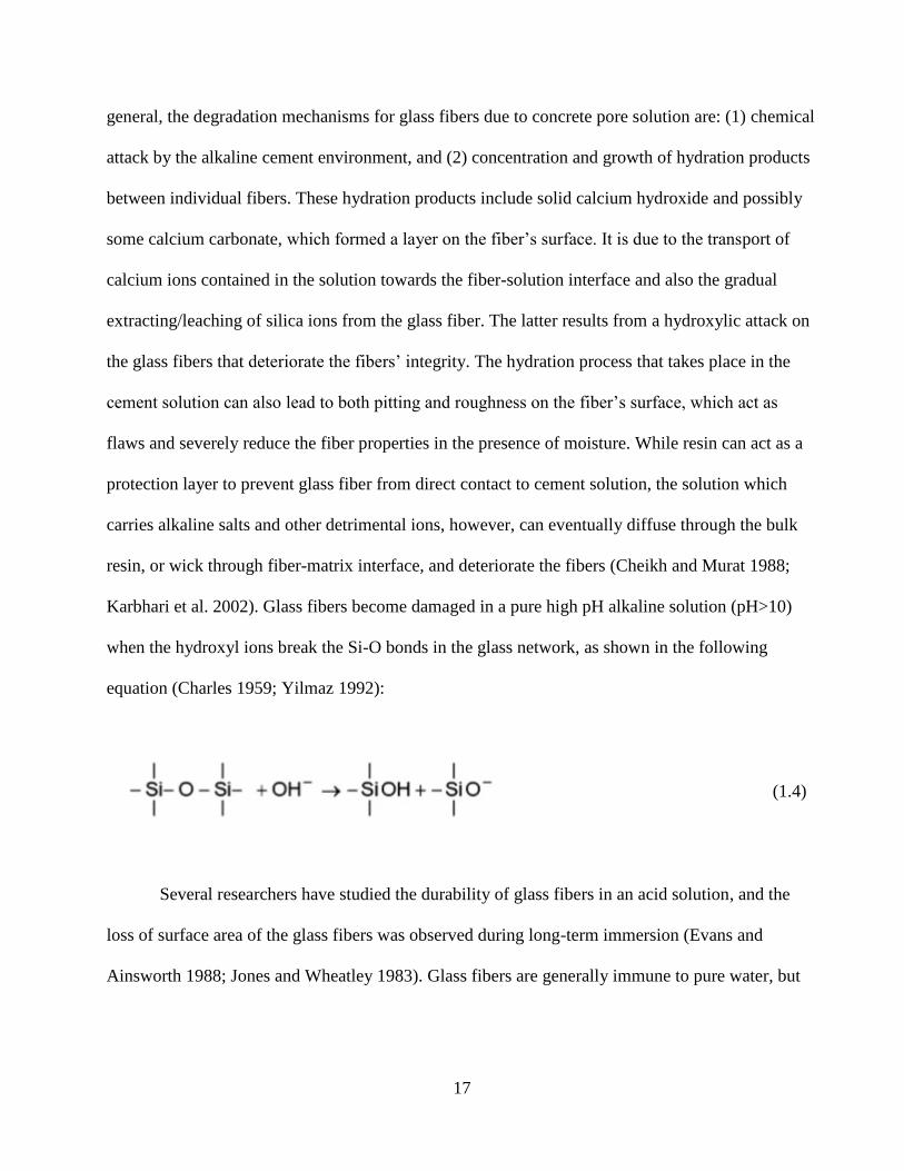
Karbhari et al. 2002). Glass fibers become damaged in a pure high pH alkaline solution (pH>10)

when the hydroxyl ions break the Si-O bonds in the glass network, as shown in the following

equation (Charles 1959; Yilmaz 1992):

(1.4)

Several researchers have studied the durability of glass fibers in an acid solution, and the

loss of surface area of the glass fibers was observed during long-term immersion (Evans and

Ainsworth 1988; Jones and Wheatley 1983). Glass fibers are generally immune to pure water, but

18

chloride ions can deteriorate glass fibers through leaching and etching (Balazs and Borosnyoi

2001).

Aramid fibers are particularly susceptible to moisture absorption while carbon fibers are

known to be inert to chemical environments and do not absorb water (Chen et al. 2007). Micelli and

Myers (2008) submerged CFRP sheets in an HCL solution for 2,000 hours and then tested in

tension. The maximum reduction measured on the strength and stiffness was only 20%, indicating

the carbon fibers had a high chemical resistance. The carbon fibers are, however, vulnerable to

electrolytic solutions. Alias and Brown (1992) showed that the carbon fiber composite materials in

a seawater (3.5% NaCl) solution and in contact with metals experienced significant damage due to

blistering and dissolution of the matrix under galvanic action.

1.6.3 Fiber/Matrix Interface

The degradation mechanism for the interface between the fiber and the matrix is quite

complicated. The interface is an inhomogeneous layer that is approximately one micron thickness.

It is the weakest bond and most vulnerable part in the composite microstructure (Chen et al. 2007).

Three degradation mechanisms of interface between fiber and matrix include: (1) matrix osmotic

cracking, (2) interfacial debonding, and (3) delamination (Bradshaw and Brinson, 1997).

1.7 Various Environmental Exposures on FRP Composite

1.7.1 Moisture

In general, moisture decreases the glass transition temperature of the polymer matrix due to

plasticization by means of interrupting Van Der Waals bonds between polymer chains. It leads to

the degradation of matrix-dominated mechanical properties of the composite (Wolff 1993). The

matrix could also be damaged by cracking and microcracking when the volume expands during

moisture absorption. Ashbee and Wyatt (1969) reported that the change of resin’s volume when

19

subjected to boiling water was initiated by swelling after the resin was immersed in water for a very

short time, but then superseded by shrinkage later. The volume shrinkage could be explained by

two possible mechanisms, either: (1) extra cross-linking was formed, increasing the resin’s density;

or (2) the low molecular weight material was leached from the bulk resin, followed by a closing-in

behavior of the adjacent polymer to fill the holes left behind by extracted molecules. The above two

mechanisms lead to a more rigid and brittle behavior for the resin, but the water would act as a

plasticizer later on, decreasing the Tg and elastic modulus of the resin if it were kept in the water

for a longer time period (Lima et al. 2009). Researchers have conducted a number of experiments to

investigate the moisture effect on durability of FRP composites. Chen et al. (2007) reported that the

continuous immersion of GFRP in a wet solution resulted in greater degradation than wet and dry

cycles. McBagonluri et al. (2000) conducted tensile tests on glass/vinylester composite coupons

that were subjected to cyclic moisture aging in both freshwater and saltwater. They found that the

quasi-static tensile strength of the FRP specimens was reduced by 24% at a moisture concentration

of 1% by weight. More importantly, this degradation was shown to be permanent and cannot be

reversible even when the sample was dried. Gentry et al. (1998) concluded that an aqueous

environmental condition affects more in strength than modulus for glass/polyester and

glass/vinylester composite materials. Tucker and Brown (1989) examined the moisture effect on the

FRP composite under high pressure to investigate the performance of FRP structures in deep sea.

They found that the high pressure did not change the diffusion rate of the composite materials. It

did, however, raise the equilibrium moisture, further deteriorating the strength and stiffness of the

composite materials.

A number of researchers have studied the impact of saltwater on an FRP composite. It was

reported that the FRP’s degradation when immersed in saltwater is more attributed to FRP’s

20

moisture content than salt concentration. It was observed that the rate of strength decrease for

samples in a saline solution is lower than that in distilled water, because the massive salt molecules

in a saline solution impede water absorption (D’Almieda 1991). A salt solution can also cause

blistering on an FRP composite’s surface due to osmotic effects (ACI 2007).

Silva et al. (2014) conducted more comprehensive durability tests on epoxy-based GFRP

and CFRP composite laminates. These composites were subjected to salt fog cycles with 5%

salinity, tap water wet/dry cycles, 5% saltwater wet/dry cycles, and freezing/thawing cycles with

10% RH. They found that saltwater wet/dry cycles reduced Tg of epoxy more severely than either

salt fog or freezing/thawing cycles. The adhesion between the fiber and the matrix degraded more

rapidly during both wet/dry cycles and salt fog cycles than it did during freezing/thawing cycles.

Thus, moisture was the primary factor, rather than either salinity or low temperatures, in degrading

the FRP composite.

1.7.2 High Temperatures

High temperatures affect the viscoelastic response of the resin, which led to the decreased

modulus (ACI 2007). The glass transition temperature (Tg) is one of the most important properties

of resin when considering environmental temperature. The resin’s mechanical properties will be

degraded dramatically if the service temperature approaches Tg. Both moisture and high

temperature have a significant effect on Tg, but depending on the materials’ curing temperature. A

reduced Tg will be observed for high-temperature-cured materials due to the plasticisation effects

of hygrothermal exposure. However, the post-cure induced by elevated temperature hygrothermal

exposure will increase Tg for low-temperature-cured materials. This increase will become greater

when the ageing temperature is enhanced (Earl and Shenoi 2004). If materials are high-temperature

cured properly, the high temperature condition deteriorates the composite material more

21

significantly than low temperature effect. Fabio et al (2012) found that CFRP laminates tested at a

temperature of +70°C, and an RH of 65% had a significant decrease in tensile strength and ultimate

strain, approximately equal to 30%, but no significant change was observed in stiffness.

1.7.3 Low Temperatures

Compared to high temperature effect, freezing/thawing cycles barely affect the ultimate

strength and strain of CFRP laminates, with only a slight decrease (9% and 13%) for 210 cycles

(Fabio et al. 2012). Miguel et al. (2006) found that exposure to freeze-thaw cycles had little effect

on the longitudinal tensile properties of the saturated FRP tubes. Low temperatures make the resin

stiffer, but the composite may suffer from internal stresses resulting from thermal coefficient

mismatch of fibers and resins (Dutta and Hui 1996). The internal stresses will cause microcracks on

the resin’s surface which induces more moisture and aggressive agents into the resin. Typically, wet

freeze-thaw conditioning deteriorates the FRP composite more severely than dry freeze-thaw

condition. While freezing/thawing cycles deteriorate composite materials, a constant freeze

temperature improves the composite’s properties. Rivera and Karbhari (2001) subjected vinylester-

based GFRP and CFRP materials to a constant freeze temperature (-10°C). They found that both the

tensile strength and the modulus increased for all of the specimens.

1.7.4 Ultraviolet (UV) Light

Surface oxidation occurs when resin materials are exposed to ultraviolet (UV) light, as

evidenced by the increase in oxygen-containing functional groups. Surface oxidation can

potentially cause degradation in mechanical properties of resin materials (Chin et al. 1997). More

specifically, UV exposure primarily affects the surface region to a depth of approximately 10

micrometers. The degradation mechanism involves cross-linking that spoils the surface’s aesthetic

appearance. The combined UV exposure and high humidity was shown to severely deteriorate the

22

FRP composite’s surface and led to reduced fracture toughness, as the flaws on the surface can

serve as stress concentrators and initiate fracture of the whole composite at stress levels much lower

than those of unexposed material portions (Ashbee 1989; Moore and Epps 1992; Underwood and

Kapusta 1991).

1.8 Accelerated Conditioning and Prediction Methodology

Currently, Fick’s law and the Arrhenius relation are the two theories most often used to

estimate the long-term performance of FRP materials, where the latter gains more popularity.

Tannous and Saadatmanesh (1998) used Fick’s law to determine the mass diffusion coefficient (D).

A number of researchers have applied the Arrhenius law to generate the prediction curve for FRP

composite structures in marine areas or those affected by deicing salt. Experiments have been

conducted on the long-term performance of concrete-filled GFRP tube cylinders and concrete

embedded GFRP bars in salt solution for up to one year (Robert and Fam 2012; Robert and

Benmokrane 2013). Elevated temperatures were used as the accelerated aging factor to accelerate

corrosion. They found that for both GFRP tubes and GFRP bars, no significant change occurred on

the microstructure of the FRP cross-section, glass transition temperature of the resin showed no

difference, and chemical structure remained basically the same for the resin. The prediction curves

revealed that the GFRP bar retained 77% of its tensile strength after 100 service years in salt water

at a mean annual temperature of 10°C, and hoop tensile strength of the GFRP tubes decreased by

30% after 48 service years at a mean annual temperature of 6°C. Several researchers have

investigated the reliability of prediction curves that are based on the Arrhenius relation. Phani and

Bose (1987) concluded that the reduction in strength of an FRP composite as a result of

hydrothermal effects is a rate process in which the temperatures influence only the rate constant.

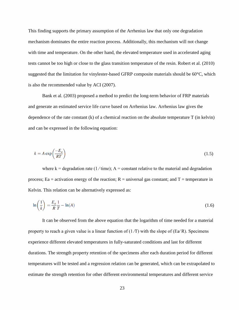
23

This finding supports the primary assumption of the Arrhenius law that only one degradation

mechanism dominates the entire reaction process. Additionally, this mechanism will not change

with time and temperature. On the other hand, the elevated temperature used in accelerated aging

tests cannot be too high or close to the glass transition temperature of the resin. Robert et al. (2010)

suggested that the limitation for vinylester-based GFRP composite materials should be 60°C, which

is also the recommended value by ACI (2007).

Bank et al. (2003) proposed a method to predict the long-term behavior of FRP materials

and generate an estimated service life curve based on Arrhenius law. Arrhenius law gives the

dependence of the rate constant (k) of a chemical reaction on the absolute temperature T (in kelvin)

and can be expressed in the following equation:

(1.5)

where k = degradation rate (1 ∕ time); A = constant relative to the material and degradation

process; Ea = activation energy of the reaction; R = universal gas constant; and T = temperature in

Kelvin. This relation can be alternatively expressed as:

(1.6)

It can be observed from the above equation that the logarithm of time needed for a material

property to reach a given value is a linear function of (1 ∕T) with the slope of (Ea∕ R). Specimens

experience different elevated temperatures in fully-saturated conditions and last for different

durations. The strength property retention of the specimens after each duration period for different

temperatures will be tested and a regression relation can be generated, which can be extrapolated to

estimate the strength retention for other different environmental temperatures and different service

24

life times. It is noted that there are limitations when applying the Arrhenius law to estimate the

long-term behavior. First, only one chemical degradation mechanism dominates the entire reaction,

and this mechanism will not change with time and temperature during exposure. Second, the

conditioning temperatures cannot be too close to the glass transition temperature of the resin

matrix, because the resin is believed to change the mode when approaching its glass transition

temperature. Finally, in order to see any noticeable change in the properties of an FRP composite as

a function of temperature, the FRP must be conditioned in an aqueous environment and not dry.

This law is powerful to predict the long-term performance of materials in a high moisture state

during their service life, and the performance of dry materials must be better.

1.9 Durability of Concrete-Filled FRP Tube (CFFT) Cylinders

Up to now, few studies have been focused on the durability of FRP confined concrete

cylinders subjected to various environmental exposures. In addition to the environmental corrosion

on the outer FRP, the confining pressure acted by the outer FRP on the concrete core is another

consideration for the hybrid system level. Both moisture and elevated temperature can cause

hydrothermal swelling of the FRP wraps. This swelling can lead to residual hoop strain in the FRP

wrap and diminish the confining effect on the concrete core. Actually, the coefficients of thermal

expansion (CTEs) for FRP composites are quite different from those of concrete or steel. The CTE

of GFRP is generally higher than that of concrete and steel, while the CTEs of CFRP and AFRP are

generally smaller than that of concrete and steel in fiber direction (ACI 2007). However, in the

transverse direction, the CTEs of GFRP, CFRP, and AFRP are all higher than that of concrete and

steel, especially for AFRP which possesses approximately a value 5-8 times higher (Balazs and

25

Borosnyoi 2001). The reduced confinement on concrete is indicated by the decreased critical stress,

ultimate strength, and ultimate strain of the hybrid system (Kshirsagar et al. 2000).

Micelli and Myers (2008) conducted durability tests on concrete cylinders that were

wrapped with either GFRP or CFRP sheets. The cylinders were subjected to either combined

freeze-thaw cycles, moisture cycles and high temperature cycles, or immersed in a NaCl solution

with 15% by mass. They found that GFRP confined concrete cylinders, after being exposed to

either environmental conditioning or a NaCl solution, exhibited a moderate decrease in ultimate

strength. The ductility, however, was significantly reduced by more than 40%. CFRP confined

concrete cylinders, however, did not show any significant change in ultimate strength, though they

did lose 30% of their axial strain after they were immersed in the NaCl solution.

Pando et al. (2002) presented ongoing research of long-term moisture effect on CFFT

cylinders. The methodology used in the study is first used to track the moisture absorption in the

FRP materials and estimate the strength of the FRP tube for a given period of time. Then, a

confinement model based on reduced tube strength and stiffness was used to evaluate the residual

strength of the CFFT piles. Fam et al. (2002) also conducted moisture effect tests on concrete-filled

GFRP piles. They submerged GFRP cylinders with two different laminate structures into

freshwater for up to one year. They noted that the degradation for GFRP cylinders were about 13 to

20%, and the degradation rate was reduced over time. Robert and Fam (2012) carried out durability

prediction experiments on GFRP tube cylinders that were subjected to saltwater immersion. It was

observed that there was no significant change on microstructure of FRP composite, and no change

on thermal or chemical structure of the epoxy matrix. They also found the hoop tensile strength of

the GFRP tube was estimated to decrease by 30% after 48 service years at a mean annual

temperature of 6°C.

26

Fam et al. (2008) conducted freezing-thawing cycle tests on both low-strength concrete and

medium-strength concrete filled FRP tubes while under sustained axial loading, and carried out

compression tests on cylinders before and after exposure. They found that sustained load and

freezing-thawing conditions increased compressive strength of the CFFT cylinders with low-

strength concrete. They proposed that both the creep effect and the dilation that occurred during the

thawing process induced extra radial strain in the concrete core, thus triggering more active

confining pressures from the outer FRP tube. These behaviors were not observed, however, in

CFFT specimens with medium-strength concrete. This was due to the brittle nature and low dilation

capacity of medium to high strength concrete. The difference between low strength concrete core

and high strength concrete core agrees well with the authors’ previous work (Mandal et al. 2005),

where the FRP tube was proved to enhance the strength and ductility more effectively on low

strength concrete than high strength concrete.

Several researchers have also studied the behavior of CFFT cylinders under mechanical

loading. Naguib and Mirmiran (2002) studied the long-time shrinkage and creep behavior of CFFT

cylinders under sustained axial loading and found that: (1) the shrinkage of the concrete core in

CFFT cylinders was quite negligible, and (2) the concrete core’s creep coefficient decreased as the

FRP tube’s elastic modulus increased.

Besides those actual experiments, the American Concrete Institute (ACI) committee 440

also attempted to quantify the degradation of the FRP composite system due to different service

environments. They provided a table of environmental reduction factors for the FRP composite

system based on fiber type and environmental exposure type (ACI 2008).

When designing FRP composite structures, FRP material properties should consider the

effect of environmental exposure that will result in a reduced value rather than data provided by

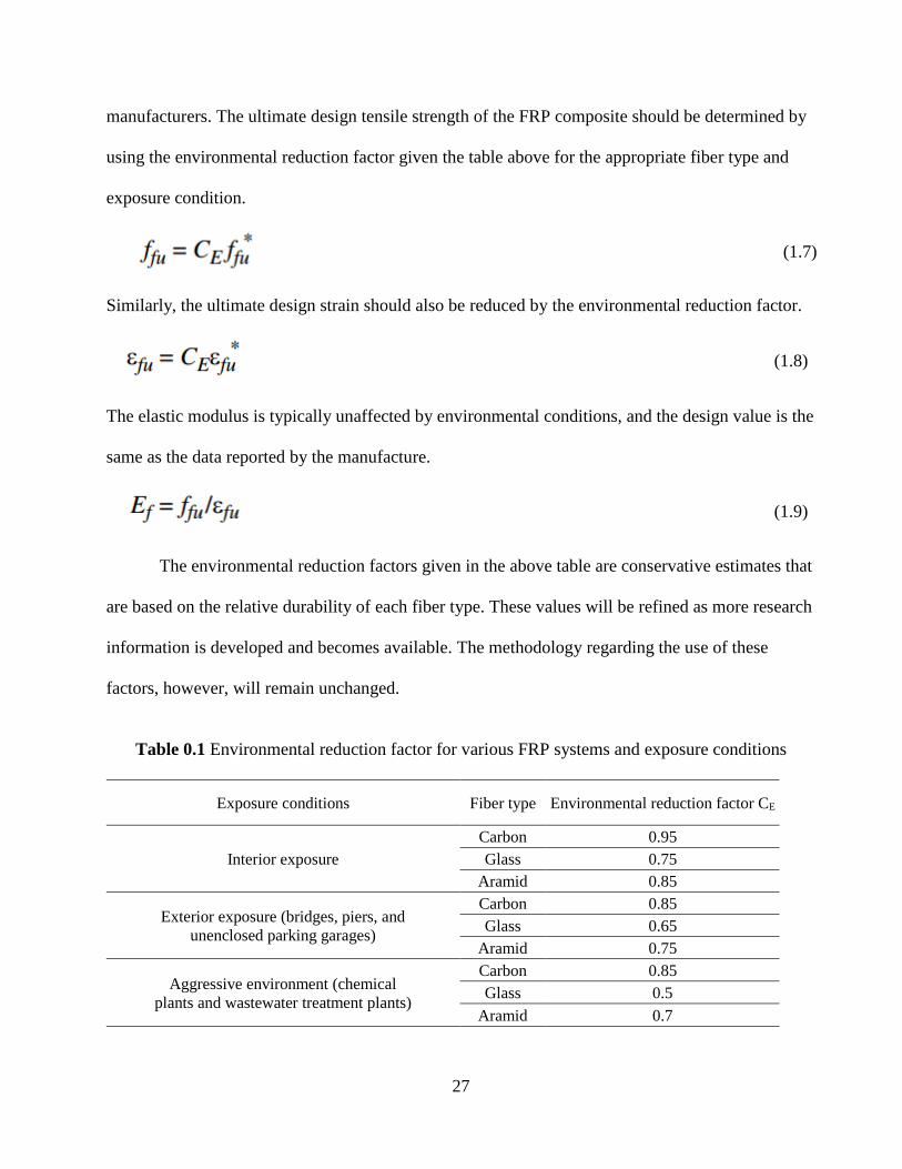
27

manufacturers. The ultimate design tensile strength of the FRP composite should be determined by

using the environmental reduction factor given the table above for the appropriate fiber type and

exposure condition.

(1.7)

Similarly, the ultimate design strain should also be reduced by the environmental reduction factor.

(1.8)

The elastic modulus is typically unaffected by environmental conditions, and the design value is the

same as the data reported by the manufacture.

(1.9)

The environmental reduction factors given in the above table are conservative estimates that

are based on the relative durability of each fiber type. These values will be refined as more research

information is developed and becomes available. The methodology regarding the use of these

factors, however, will remain unchanged.

Table 0.1 Environmental reduction factor for various FRP systems and exposure conditions

Exposure conditions Fiber type Environmental reduction factor CE

Interior exposure

Carbon 0.95

Glass 0.75

Aramid 0.85

Exterior exposure (bridges, piers, and

unenclosed parking garages)

Carbon 0.85

Glass 0.65

Aramid 0.75

Aggressive environment (chemical

plants and wastewater treatment plants)

Carbon 0.85

Glass 0.5

Aramid 0.7

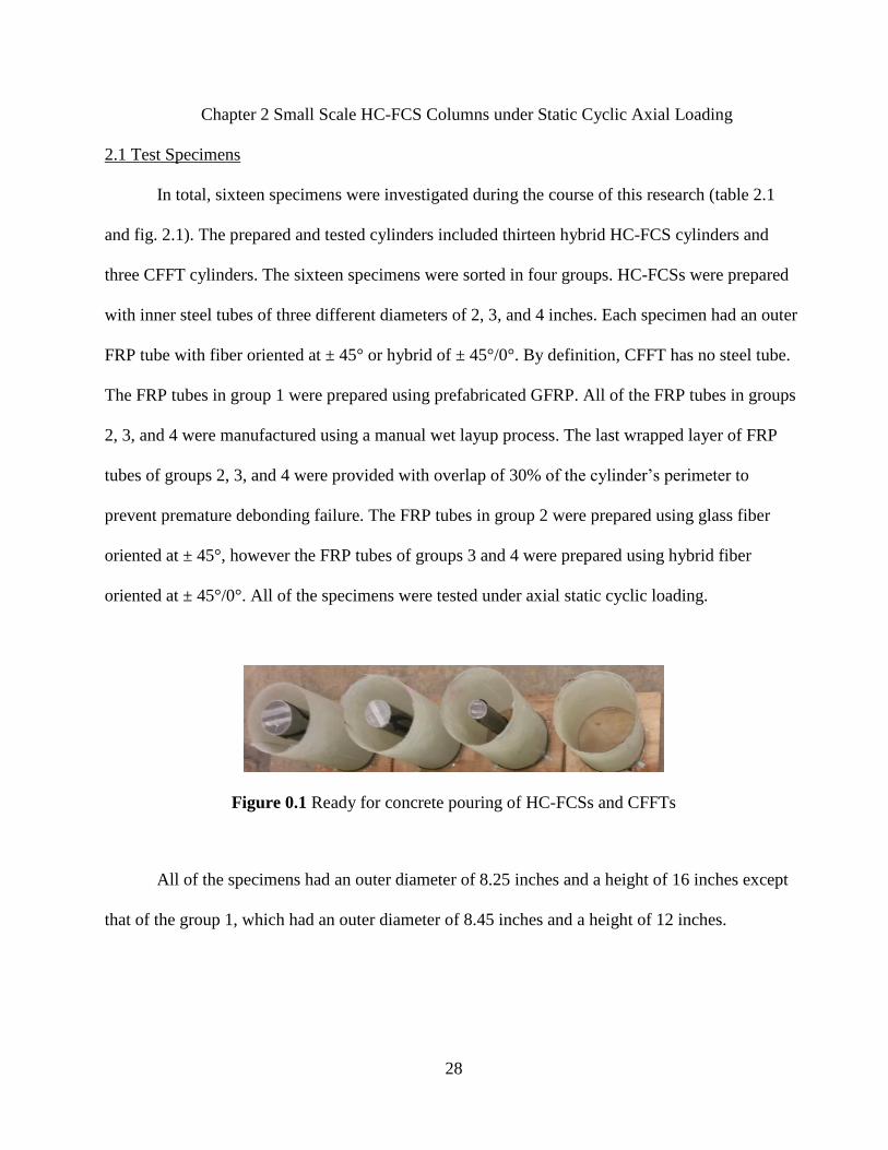
28

Chapter 2 Small Scale HC-FCS Columns under Static Cyclic Axial Loading

2.1 Test Specimens

In total, sixteen specimens were investigated during the course of this research (table 2.1

and fig. 2.1). The prepared and tested cylinders included thirteen hybrid HC-FCS cylinders and

three CFFT cylinders. The sixteen specimens were sorted in four groups. HC-FCSs were prepared

with inner steel tubes of three different diameters of 2, 3, and 4 inches. Each specimen had an outer

FRP tube with fiber oriented at ± 45° or hybrid of ± 45°/0°. By definition, CFFT has no steel tube.

The FRP tubes in group 1 were prepared using prefabricated GFRP. All of the FRP tubes in groups

2, 3, and 4 were manufactured using a manual wet layup process. The last wrapped layer of FRP

tubes of groups 2, 3, and 4 were provided with overlap of 30% of the cylinder’s perimeter to

prevent premature debonding failure. The FRP tubes in group 2 were prepared using glass fiber

oriented at ± 45°, however the FRP tubes of groups 3 and 4 were prepared using hybrid fiber

oriented at ± 45°/0°. All of the specimens were tested under axial static cyclic loading.

Figure 0.1 Ready for concrete pouring of HC-FCSs and CFFTs

All of the specimens had an outer diameter of 8.25 inches and a height of 16 inches except

that of the group 1, which had an outer diameter of 8.45 inches and a height of 12 inches.

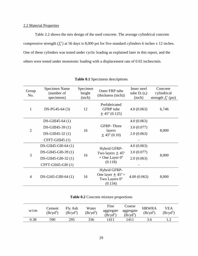
29

2.2 Material Properties

Table 2.2 shows the mix design of the used concrete. The average cylindrical concrete

compressive strength (𝑓𝑐′) at 56 days is 8,000 psi for five standard cylinders 6 inches x 12 inches.

One of these cylinders was tested under cyclic loading as explained later in this report, and the

others were tested under monotonic loading with a displacement rate of 0.02 inches/min.

Table 0.1 Specimens descriptions

Group

No.

Specimen Name

(number of

specimens)

Specimen

height

(inch)

Outer FRP tube

(thickness (inch))

Inner steel

tube Di (ts)

(inch)

Concrete

cylindrical

strength 𝑓𝑐′ (psi)

1 DS-PG45-64 (3) 12

Prefabricated

GFRP tube

± 45o (0.125)

4.0 (0.063) 6,746

2

DS-GIII45-64 (1)

16

GFRP- Three

layers

± 45o (0.10)

4.0 (0.063)

8,000 DS-GIII45-39 (1) 3.0 (0.077)

DS-GIII45-32 (1) 2.0 (0.063)

CFFT-GIII45 (1) -

3

DS-GII45-GI0-64 (1)

16

Hybrid GFRP-

Two layers ± 45o

+ One Layer 0o

(0.118)

4.0 (0.063)

8,000 DS-GII45-GI0-39 (1) 3.0 (0.077)

DS-GII45-GI0-32 (1) 2.0 (0.063)

CFFT-GII45-GI0 (1) -

4 DS-GI45-GII0-64 (1) 16

Hybrid GFRP-

One layer ± 45o +

Two Layers 0o

(0.134)

4.00 (0.063) 8,000

Table 0.2 Concrete mixture proportions

w/cm Cement

(lb/yd3)

Fly Ash

(lb/yd3)

Water

(lb/yd3)

Fine

aggregate

(lb/yd3)

Coarse

aggregate

(lb/yd3)

HRWRA

(lb/yd3)

VEA

(lb/yd3)

0.38 590 295 336 1411 1411 3.6 1.2

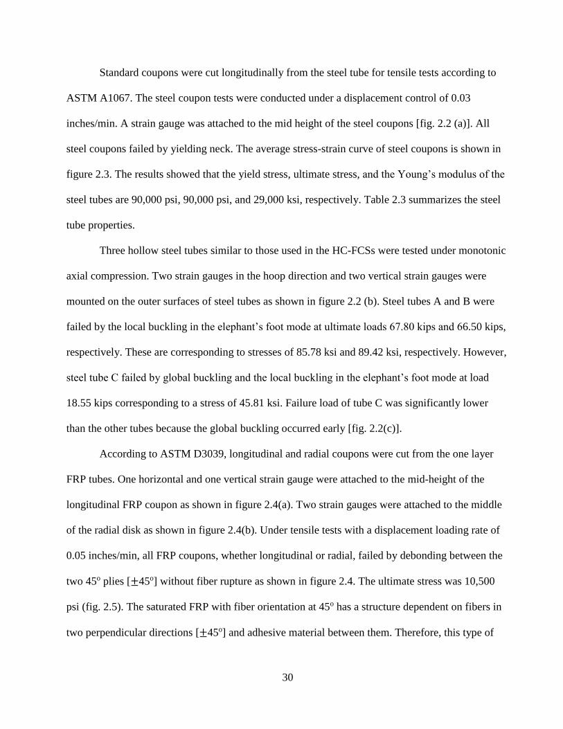
30

Standard coupons were cut longitudinally from the steel tube for tensile tests according to

ASTM A1067. The steel coupon tests were conducted under a displacement control of 0.03

inches/min. A strain gauge was attached to the mid height of the steel coupons [fig. 2.2 (a)]. All

steel coupons failed by yielding neck. The average stress-strain curve of steel coupons is shown in

figure 2.3. The results showed that the yield stress, ultimate stress, and the Young’s modulus of the

steel tubes are 90,000 psi, 90,000 psi, and 29,000 ksi, respectively. Table 2.3 summarizes the steel

tube properties.

Three hollow steel tubes similar to those used in the HC-FCSs were tested under monotonic

axial compression. Two strain gauges in the hoop direction and two vertical strain gauges were

mounted on the outer surfaces of steel tubes as shown in figure 2.2 (b). Steel tubes A and B were

failed by the local buckling in the elephant’s foot mode at ultimate loads 67.80 kips and 66.50 kips,

respectively. These are corresponding to stresses of 85.78 ksi and 89.42 ksi, respectively. However,

steel tube C failed by global buckling and the local buckling in the elephant’s foot mode at load

18.55 kips corresponding to a stress of 45.81 ksi. Failure load of tube C was significantly lower

than the other tubes because the global buckling occurred early [fig. 2.2(c)].

According to ASTM D3039, longitudinal and radial coupons were cut from the one layer

FRP tubes. One horizontal and one vertical strain gauge were attached to the mid-height of the

longitudinal FRP coupon as shown in figure 2.4(a). Two strain gauges were attached to the middle

of the radial disk as shown in figure 2.4(b). Under tensile tests with a displacement loading rate of

0.05 inches/min, all FRP coupons, whether longitudinal or radial, failed by debonding between the

two 45o plies [±45o] without fiber rupture as shown in figure 2.4. The ultimate stress was 10,500

psi (fig. 2.5). The saturated FRP with fiber orientation at 45o has a structure dependent on fibers in

two perpendicular directions [±45o] and adhesive material between them. Therefore, this type of

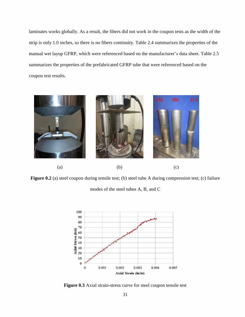
31

laminates works globally. As a result, the fibers did not work in the coupon tests as the width of the

strip is only 1.0 inches, so there is no fibers continuity. Table 2.4 summarizes the properties of the

manual wet layup GFRP, which were referenced based on the manufacturer’s data sheet. Table 2.5

summarizes the properties of the prefabricated GFRP tube that were referenced based on the

coupon test results.

(a)

(b)

(c)

Figure 0.2 (a) steel coupon during tensile test; (b) steel tube A during compression test; (c) failure

modes of the steel tubes A, B, and C

Figure 0.3 Axial strain-stress curve for steel coupon tensile test

[A] [B] [C]

32

Table 0.3 Properties of steel tubes

Material Young’s

modulus, E (ksi)

Yield stress

(psi)

Ultimate stress

(psi) Ultimate strain

Steel 29,000 90,000 90,000 0.40 %

Table 0.4 Properties of saturated FRP according to manufacturer’s data

Material

Nominal

thickness/layer

(inch)

Young’s

modulus, E (ksi)

Tensile strength

(psi) Ultimate strain

GFRP-45o 0.034 2,700 40,500 1.50 %

GFRP-0o 0.050 3,790 83,400 2.20 %

Table 0.5 Properties of the prefabricated GFRP tubes

Material

Nominal

thickness/layer

(inch)

Hoop Young’s

modulus, E

(ksi)

Hoop tensile

strength (psi)

Axial

Young’s

modulus, E

(ksi)

Axial tensile

strength (psi)

Prefabricated

GFRP 0.125 2,028 21,350 1,523 8,430

(a)

(b)

Figure 0.4 (a) Longitudinal FRP coupon; (b) radial FRP coupon

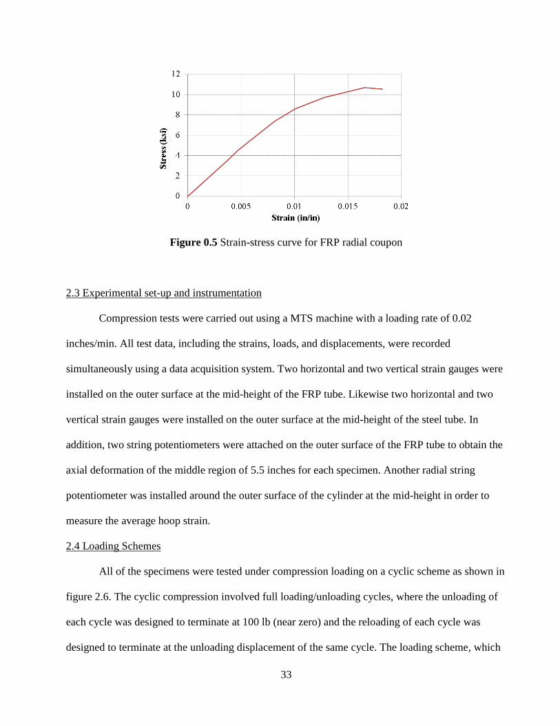
33

Figure 0.5 Strain-stress curve for FRP radial coupon

2.3 Experimental set-up and instrumentation

Compression tests were carried out using a MTS machine with a loading rate of 0.02

inches/min. All test data, including the strains, loads, and displacements, were recorded

simultaneously using a data acquisition system. Two horizontal and two vertical strain gauges were

installed on the outer surface at the mid-height of the FRP tube. Likewise two horizontal and two

vertical strain gauges were installed on the outer surface at the mid-height of the steel tube. In

addition, two string potentiometers were attached on the outer surface of the FRP tube to obtain the

axial deformation of the middle region of 5.5 inches for each specimen. Another radial string

potentiometer was installed around the outer surface of the cylinder at the mid-height in order to

measure the average hoop strain.

2.4 Loading Schemes

All of the specimens were tested under compression loading on a cyclic scheme as shown in

figure 2.6. The cyclic compression involved full loading/unloading cycles, where the unloading of

each cycle was designed to terminate at 100 lb (near zero) and the reloading of each cycle was

designed to terminate at the unloading displacement of the same cycle. The loading scheme, which

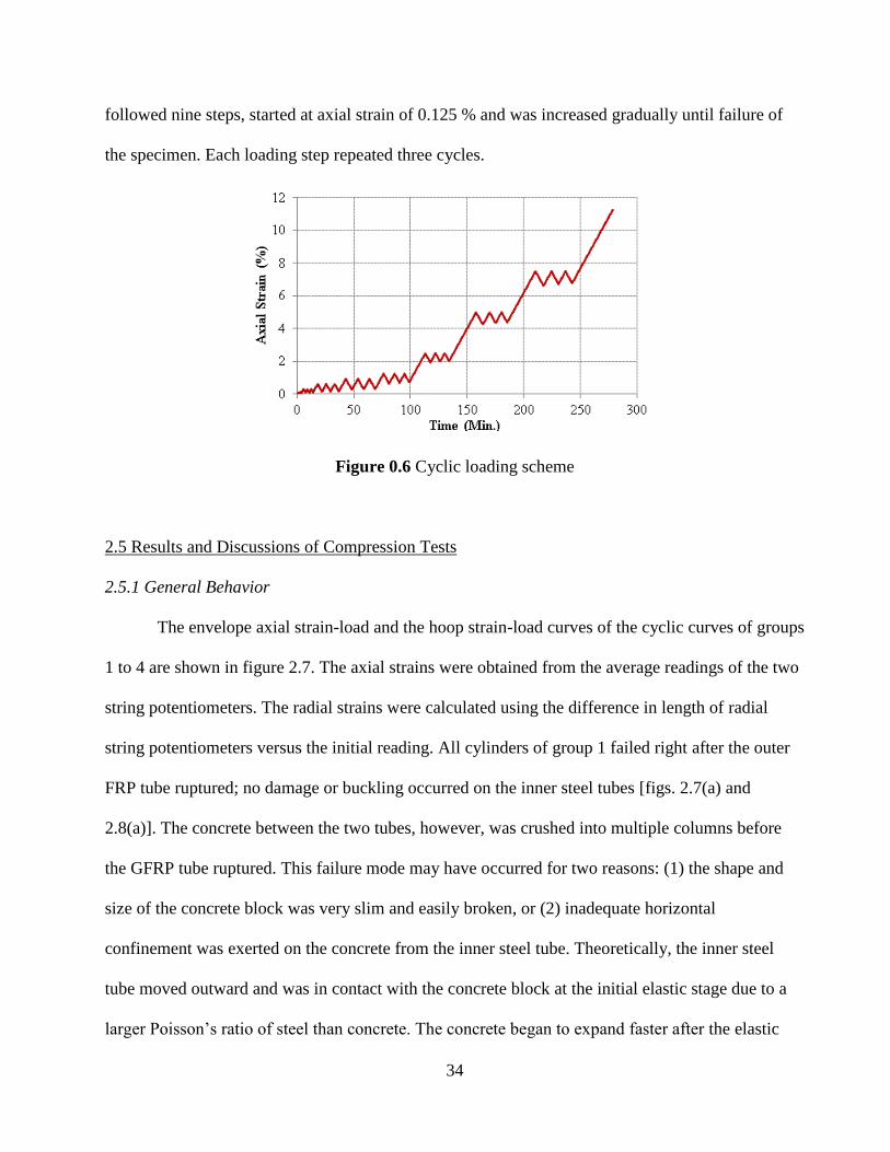
34

followed nine steps, started at axial strain of 0.125 % and was increased gradually until failure of

the specimen. Each loading step repeated three cycles.

Figure 0.6 Cyclic loading scheme

2.5 Results and Discussions of Compression Tests

2.5.1 General Behavior

The envelope axial strain-load and the hoop strain-load curves of the cyclic curves of groups

1 to 4 are shown in figure 2.7. The axial strains were obtained from the average readings of the two

string potentiometers. The radial strains were calculated using the difference in length of radial

string potentiometers versus the initial reading. All cylinders of group 1 failed right after the outer

FRP tube ruptured; no damage or buckling occurred on the inner steel tubes [figs. 2.7(a) and

2.8(a)]. The concrete between the two tubes, however, was crushed into multiple columns before

the GFRP tube ruptured. This failure mode may have occurred for two reasons: (1) the shape and

size of the concrete block was very slim and easily broken, or (2) inadequate horizontal

confinement was exerted on the concrete from the inner steel tube. Theoretically, the inner steel

tube moved outward and was in contact with the concrete block at the initial elastic stage due to a

larger Poisson’s ratio of steel than concrete. The concrete began to expand faster after the elastic

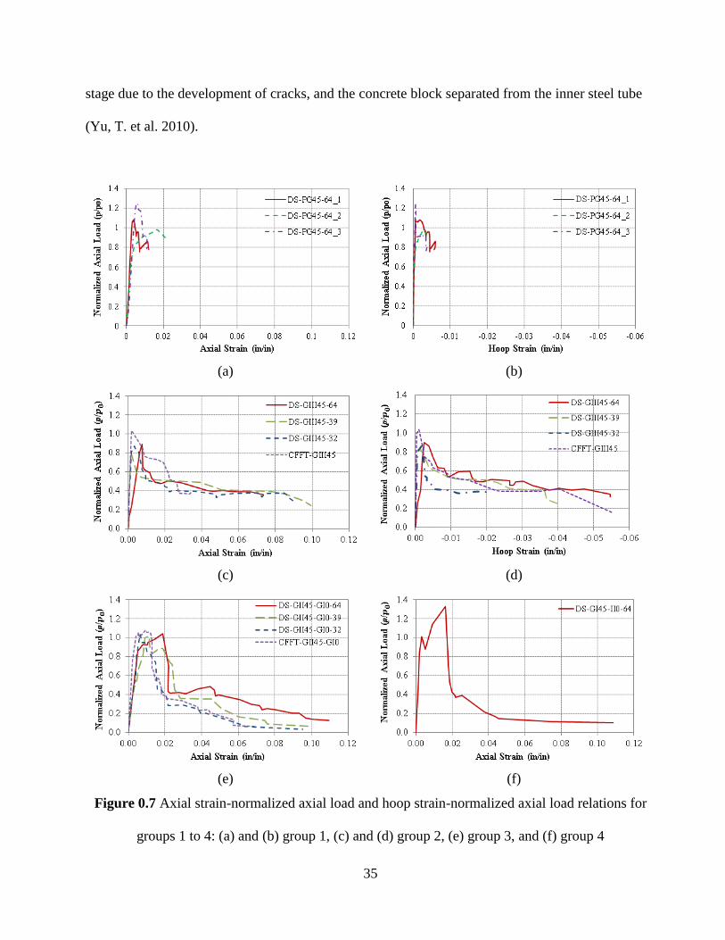
35

stage due to the development of cracks, and the concrete block separated from the inner steel tube

(Yu, T. et al. 2010).

(a) (b)

(c) (d)

(e) (f)

Figure 0.7 Axial strain-normalized axial load and hoop strain-normalized axial load relations for

groups 1 to 4: (a) and (b) group 1, (c) and (d) group 2, (e) group 3, and (f) group 4

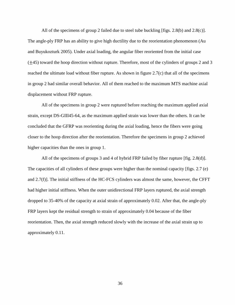
36

All of the specimens of group 2 failed due to steel tube buckling [figs. 2.8(b) and 2.8(c)].

The angle-ply FRP has an ability to give high ductility due to the reorientation phenomenon (Au

and Buyukozturk 2005). Under axial loading, the angular fiber reoriented from the initial case

(±45) toward the hoop direction without rupture. Therefore, most of the cylinders of groups 2 and 3

reached the ultimate load without fiber rupture. As shown in figure 2.7(c) that all of the specimens

in group 2 had similar overall behavior. All of them reached to the maximum MTS machine axial

displacement without FRP rupture.

All of the specimens in group 2 were ruptured before reaching the maximum applied axial

strain, except DS-GIII45-64, as the maximum applied strain was lower than the others. It can be

concluded that the GFRP was reorienting during the axial loading, hence the fibers were going

closer to the hoop direction after the reorientation. Therefore the specimens in group 2 achieved

higher capacities than the ones in group 1.

All of the specimens of groups 3 and 4 of hybrid FRP failed by fiber rupture [fig. 2.8(d)].

The capacities of all cylinders of these groups were higher than the nominal capacity [figs. 2.7 (e)

and 2.7(f)]. The initial stiffness of the HC-FCS cylinders was almost the same, however, the CFFT

had higher initial stiffness. When the outer unidirectional FRP layers ruptured, the axial strength

dropped to 35-40% of the capacity at axial strain of approximately 0.02. After that, the angle-ply

FRP layers kept the residual strength to strain of approximately 0.04 because of the fiber

reorientation. Then, the axial strength reduced slowly with the increase of the axial strain up to

approximately 0.11.

37

(a)

(b)

(c)

(d)

Figure 0.8 (a) Group 1 failed specimen, (b) Group 2 failed specimen (c) Steel tube local

buckling, (d) Group 3 failed specimen

2.5.2 FRP Axial-Hoop Strains Relation

The relation between the axial and hoop strain is considered the key parameter that controls

the effectiveness of the confinement of FRP. As all specimens were similar in the relation of the

axial and hoop strains, the specimen DS-GIII45-32 was considered to represent this relation. Figure

2.9 shows the axial strain-axial load curve and the hoop strain-axial load curve of such a specimen.

It was noted that the axial and hoop strains were increasing simultaneously. During the first cycles,

before ultimate load, the hoop and axial strains were increasing at a high rate. This means the

expansion of the concrete under axial loading was outward only. At ultimate load, the failure

occurred due to the steel tube local buckling. After the local buckling of the steel tube and up to

axial strain of 10,000 microstrain, the hoop strain was increasing with a low rate. It means the

concrete expansion was in the outward and inward directions. After the axial strain of 10,000

microstrain, the effect of local buckling almost stopped as the local buckling occurred at many

places in the steel. Therefore, the load slightly increased and the hoop strain was increasing with a

moderate rate up to the maximum applied strain.

38

Figure 0.9 Axial load-strain curve of DS-GIII45-32

2.5.3 Local Buckling of the Steel Tubes

The diameter-to-thickness (Di/ts) ratio is a very significant parameter for HC-FCS columns.

Researchers studied HC-FCS columns with D/t ratio (Ozbakkaloglu 2014, Yu 2010 and 2004, and

Wong 2007), as listed in table 2.6. In general in the previous studies, an increase in capacity for

such cylinders was achieved, or at least there was no reduction in capacity. Hence, this report

presents higher values of the Di/ts ratio, starting with 32 and going up to 64. The capacity of the

tested cylinders ranged by factors of 0.76 to 1.30 from the nominal capacity Po, which was

calculated as follows (AASHTO-LRFD 2012):

𝑃𝑜 = 𝐴𝑠𝑓𝑦 + 0.85 𝑓𝑐′(𝐴𝑐 − 𝐴𝑠) (2.1)

where As = the cross-sectional area of the steel tube or the longitudinal steel reinforcements, Ac = the

cross-sectional area of the concrete column, 𝑓𝑦 = the yield stress of the steel tube or the longitudinal

steel reinforcements, and 𝑓𝑐′ = the cylindrical concrete’s unconfined compressive stress.

39

The reduction can be explained by the steel local buckling. However, the vertical strain in

the steel tubes of the tested cylinders before local buckling was around 600-800 microstrain, which

was a very low value. That exhibited the low contribution of the steel tube in axial capacity and

hence a reduction in capacity occurred.

Normalized Di/ts can be defined as the ratio between the Di/ts to the Di/ts of AISC manual

for the steel hollow section under compression as per the following equation:

Normalized (Di

ts⁄ ) =

Dits

⁄ /(0.07 E

Fy) (2.2)

The local buckling occurs when the Di/ts ratio is higher than that of the AISC manual value.

The Di/ts ratio for the tested cylinder relative to that of the AISC manual value was between 1.37

and 2.74. In literature relative to the AISC manual, however, the ratio in the cylinders was lower

than 1.00, as shown in figure 2.10. That explains why local buckling occurred in the tested

cylinders, even in the cylinders with steel tubes, when the Di/ts ratio was equal to 32. According to

these results presented in this report, the contribution of the steel tube in the nominal capacity

calculation should be adjusted. Therefore, this research is continuing for this scope.

Figure 0.10 Actual steel diameter-thickness ratios relative to the AISC manual value versus

increase in capacity

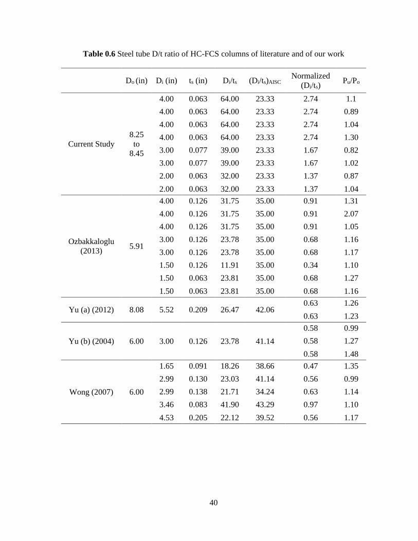
40

Table 0.6 Steel tube D/t ratio of HC-FCS columns of literature and of our work

Do (in) Di (in) ts (in) Di/ts (Di/ts)AISC Normalized

(Di/ts) Pu/Po

Current Study

8.25

to

8.45

4.00 0.063 64.00 23.33 2.74 1.1

4.00 0.063 64.00 23.33 2.74 0.89

4.00 0.063 64.00 23.33 2.74 1.04

4.00 0.063 64.00 23.33 2.74 1.30

3.00 0.077 39.00 23.33 1.67 0.82

3.00 0.077 39.00 23.33 1.67 1.02

2.00 0.063 32.00 23.33 1.37 0.87

2.00 0.063 32.00 23.33 1.37 1.04

Ozbakkaloglu

(2013) 5.91

4.00 0.126 31.75 35.00 0.91 1.31

4.00 0.126 31.75 35.00 0.91 2.07

4.00 0.126 31.75 35.00 0.91 1.05

3.00 0.126 23.78 35.00 0.68 1.16

3.00 0.126 23.78 35.00 0.68 1.17

1.50 0.126 11.91 35.00 0.34 1.10

1.50 0.063 23.81 35.00 0.68 1.27

1.50 0.063 23.81 35.00 0.68 1.16

Yu (a) (2012) 8.08 5.52 0.209 26.47 42.06 0.63 1.26

0.63 1.23

Yu (b) (2004) 6.00 3.00 0.126 23.78 41.14

0.58 0.99

0.58 1.27

0.58 1.48

Wong (2007) 6.00

1.65 0.091 18.26 38.66 0.47 1.35

2.99 0.130 23.03 41.14 0.56 0.99

2.99 0.138 21.71 34.24 0.63 1.14

3.46 0.083 41.90 43.29 0.97 1.10

4.53 0.205 22.12 39.52 0.56 1.17

41

Chapter 3 Large Scale HC-FCS Columns under Axial-Flexural Loading

3.1 Test Specimens

Four large-scale columns were tested as free cantilevers under both constant axial

compression load and cyclic lateral load. Each column had a circular cross-section with an outer

diameter (Do) of 24 inches and a height of 80 inches (fig. 3.1). The lateral load was applied at a

height (H) of 95 inches measured from the top of the footing, resulting in shear-span-to-depth ratio

of approximately 4.0. The first column was a conventional reinforced concrete (RC) column and

the other columns were HC-FCS columns. Table 5.1 summarizes the columns’ variables.

The columns’ label used in the current experimental work consisted of three segments. The

first segment is a letter F referring to flexural testing, followed by the column’s height-to-outer

diameter ratio (H/Do). The second segment refers to the column’s outer diameter (Do) in inches.

The third segment refers to the GFRP matrix using E for epoxy and P for Iso-Polyster base

matrices; this is followed by the GFRP thickness in 1/8 inch, steel thickness in 1/8 inch, and

concrete wall thickness in inches. In the case of reinforced concrete column, the third segment is

replaced with RC.

The F4-24-RC column had a longitudinal reinforcement of 8#7 corresponding to

approximately 1.0% of the concrete cross-sectional area and it had a transverse spiral reinforcement

of #4 @ 3 inches corresponding to volumetric reinforcement ratio of 1.0%. The concrete cover

beyond the spiral reinforcement was 0.5 inches [fig. 3.1(a)].

The F4-24-E324 column consisted of an outer filament wound GFRP tube with a wall

thickness (tFRP) of 0.375 inches, an inner steel tube with an outer diameter (Di) of 16 inches, a wall

thickness (ts) of 0.25 inches with a steel tube diameter-to-thickness (Di/ts) ratio of 64, and a

concrete wall thickness (tc) of 4 inches [fig. 3.1(b)]. The F4-24-P124 column was similar to the F4-

42

24-E324 except the outer filament GFRP tube was made with a matrix of Iso-polyester with a wall

thickness of 0.125 inches [fig. 3.1(c)]. The F4-24-E344 column was similar to the F4-24-E324

except the thickness of the inner steel tube was 0.5 inches [fig. 3.1(d)]. The inner steel tube of all of

the HC-FCS columns was extended inside the footing and the column loading stub using an

embedded length (Le) of 25 inches representing 1.6 Di, while the FRP tube was stopped at the top

of the footing and the bottom of the column’s loading stub. The steel tube was hollow inside. All

HC-FCS columns did not include any shear or flexure reinforcement except the steel tube.

Each column’s footing had length, width, and thickness of 60 inches, 48 inches, and 34

inches, respectively. The footing of the F4-24-RC column had bottom reinforcements of 7#7, top

reinforcements of 4#7, and shear reinforcement of #4 @ 2.5 inches [fig. 3.1(a)]. The footing of the

columns F4-24-E324 and F4-24-P124 had bottom reinforcements of 7#7, top reinforcements of

6#7, and shear reinforcement of #4 @ 2.5 inches [figs. 3.1(b) and 3.1(c)]. The footing of the

column F4-24-E344 had bottom reinforcements of 7#8, top reinforcements of 6#8, and shear

reinforcement of #4 @ 2.5 inches [fig. 3.1(d)].

Table 5.2 summarizes the concrete mixture proportions of the columns’ components. Pea

gravel of maximum aggregate size of 3/8 inches and high range water reducers (HRWR) were used

for the columns only to increase the workability. Table 5.3 summarizes the unconfined concrete

cylindrical strengths (𝑓𝑐′) of the columns and the footings at 28 days and the days of the tests. Table

5.4 summarizes the properties of the steel rebars and tubes, used during this experimental work,

based on the manufacturers’ data sheets. Table 5.5 summarizes the properties of the FRP tubes,

used during this experimental work, based on the manufacturers’ data sheets.

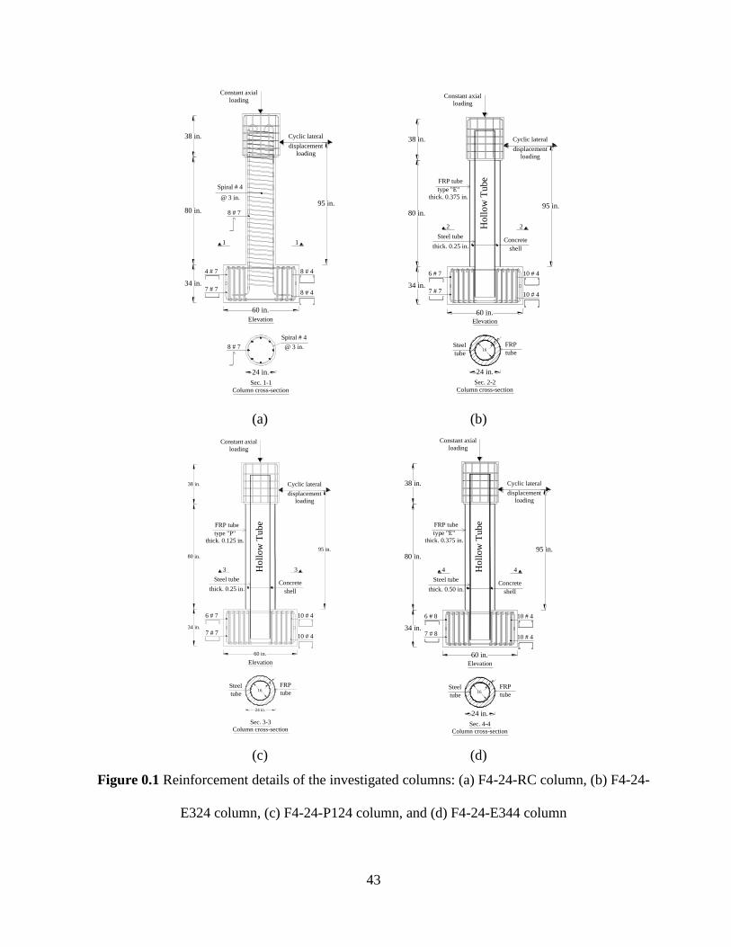
43

(a) (b)

(c) (d)

Figure 0.1 Reinforcement details of the investigated columns: (a) F4-24-RC column, (b) F4-24-

E324 column, (c) F4-24-P124 column, and (d) F4-24-E344 column

8 # 7

Spiral # 4

11

Elevation

7 # 7

4 # 7 8 # 4

8 # 4

Cyclic lateral

95 in.

8 # 7

Sec. 1-1

Column cross-section

Spiral # 4

24 in.

60 in.

34 in.

38 in.

80 in.

@ 3 in.

displacement

loading

@ 3 in.

Constant axial

loading

Ho

llo

w T

ubeFRP tube

22

7 # 7

6 # 7 10 # 4

10 # 4

Elevation

16

Sec. 2-2


24 in.

60 in.

4

34 in.

38 in.

80 in.

Cyclic lateral

95 in.

type "E"

thick. 0.375 in.

Steel tube

thick. 0.25 in.Concrete

shell

Steel

tube

FRP

tube

displacement

loading

Constant axial

loading

Ho

llo

w T

ub

e

33

Concrete

7 # 7

6 # 7 10 # 4

10 # 4

Elevation

16

Sec. 3-3


24 in.

60 in.

4

34 in.

38 in.

80 in.

Cyclic lateral

95 in.

Steel tube

thick. 0.25 in. shell

Steel

tube

FRP

tube

displacement

loading

Constant axial

loading

FRP tube

type "P"

thick. 0.125 in.

Ho

llo

w T

ub

e

44

7 # 8

6 # 8 10 # 4

10 # 4

Elevation

16

Sec. 4-4


24 in.

60 in.

4

34 in.

38 in.

80 in.

Cyclic lateral

95 in.

Steel tube

thick. 0.50 in.Concrete

shell

Steel

tube

FRP

tube

displacement

loading

Constant axial

loading

FRP tube

type "E"

thick. 0.375 in.

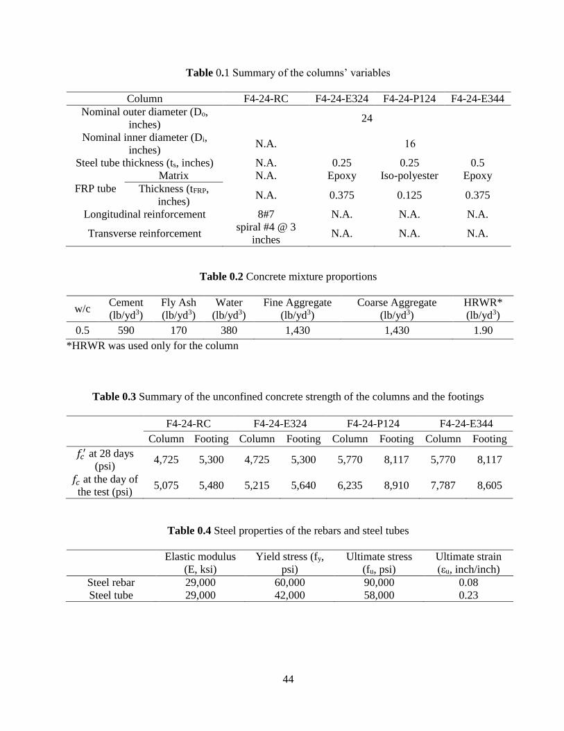
44

Table 0.1 Summary of the columns’ variables

Column F4-24-RC F4-24-E324 F4-24-P124 F4-24-E344

Nominal outer diameter (Do,

inches) 24

Nominal inner diameter (Di,

inches) N.A. 16

Steel tube thickness (ts, inches) N.A. 0.25 0.25 0.5

FRP tube

Matrix N.A. Epoxy Iso-polyester Epoxy

Thickness (tFRP,

inches) N.A. 0.375 0.125 0.375

Longitudinal reinforcement 8#7 N.A. N.A. N.A.

Transverse reinforcement spiral #4 @ 3

inches N.A. N.A. N.A.

Table 0.2 Concrete mixture proportions

w/c Cement

(lb/yd3)

Fly Ash

(lb/yd3)

Water

(lb/yd3)

Fine Aggregate

(lb/yd3)

Coarse Aggregate

(lb/yd3)

HRWR*

(lb/yd3)

0.5 590 170 380 1,430 1,430 1.90

*HRWR was used only for the column

Table 0.3 Summary of the unconfined concrete strength of the columns and the footings

F4-24-RC F4-24-E324 F4-24-P124 F4-24-E344

Column Footing Column Footing Column Footing Column Footing

𝑓𝑐′ at 28 days

(psi) 4,725 5,300 4,725 5,300 5,770 8,117 5,770 8,117

𝑓𝑐 at the day of

the test (psi) 5,075 5,480 5,215 5,640 6,235 8,910 7,787 8,605

Table 0.4 Steel properties of the rebars and steel tubes

Elastic modulus

(E, ksi)

Yield stress (fy,

psi)

Ultimate stress

(fu, psi)

Ultimate strain

(εu, inch/inch)

Steel rebar 29,000 60,000 90,000 0.08

Steel tube 29,000 42,000 58,000 0.23

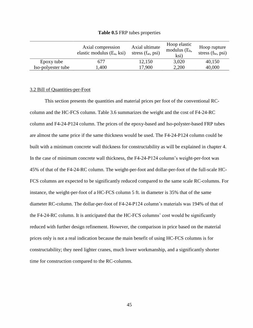
45

Table 0.5 FRP tubes properties

Axial compression

elastic modulus (Ea, ksi)

Axial ultimate

stress (far, psi)

Hoop elastic

modulus (Eh,

ksi)

Hoop rupture

stress (fhr, psi)

Epoxy tube 677 12,150 3,020 40,150

Iso-polyester tube 1,400 17,900 2,200 40,000

3.2 Bill of Quantities-per-Foot

This section presents the quantities and material prices per foot of the conventional RC-

column and the HC-FCS column. Table 3.6 summarizes the weight and the cost of F4-24-RC

column and F4-24-P124 column. The prices of the epoxy-based and Iso-polyster-based FRP tubes

are almost the same price if the same thickness would be used. The F4-24-P124 column could be

built with a minimum concrete wall thickness for constructability as will be explained in chapter 4.

In the case of minimum concrete wall thickness, the F4-24-P124 column’s weight-per-foot was

45% of that of the F4-24-RC column. The weight-per-foot and dollar-per-foot of the full-scale HC-

FCS columns are expected to be significantly reduced compared to the same scale RC-columns. For

instance, the weight-per-foot of a HC-FCS column 5 ft. in diameter is 35% that of the same

diameter RC-column. The dollar-per-foot of F4-24-P124 column’s materials was 194% of that of

the F4-24-RC column. It is anticipated that the HC-FCS columns’ cost would be significantly

reduced with further design refinement. However, the comparison in price based on the material

prices only is not a real indication because the main benefit of using HC-FCS columns is for

constructability; they need lighter cranes, much lower workmanship, and a significantly shorter

time for construction compared to the RC-columns.

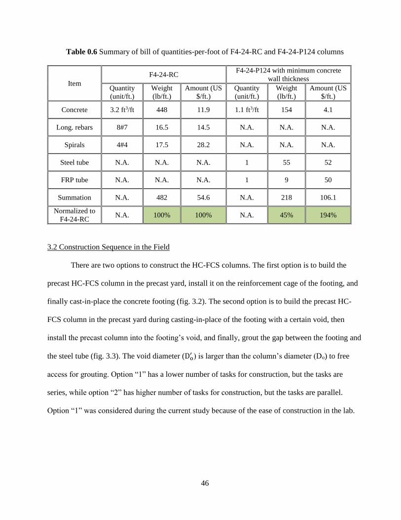
46

Table 0.6 Summary of bill of quantities-per-foot of F4-24-RC and F4-24-P124 columns

Item

F4-24-RC F4-24-P124 with minimum concrete

wall thickness

Quantity

(unit/ft.)

Weight

(lb/ft.)

Amount (US

$/ft.)

Quantity

(unit/ft.)

Weight

(lb/ft.)

Amount (US

$/ft.)

Concrete 3.2 ft3/ft 448 11.9 1.1 ft3/ft 154 4.1

Long. rebars 8#7 16.5 14.5 N.A. N.A. N.A.

Spirals 4#4 17.5 28.2 N.A. N.A. N.A.

Steel tube N.A. N.A. N.A. 1 55 52

FRP tube N.A. N.A. N.A. 1 9 50

Summation N.A. 482 54.6 N.A. 218 106.1

Normalized to

F4-24-RC N.A. 100% 100% N.A. 45% 194%

3.2 Construction Sequence in the Field

There are two options to construct the HC-FCS columns. The first option is to build the

precast HC-FCS column in the precast yard, install it on the reinforcement cage of the footing, and

finally cast-in-place the concrete footing (fig. 3.2). The second option is to build the precast HC-

FCS column in the precast yard during casting-in-place of the footing with a certain void, then

install the precast column into the footing’s void, and finally, grout the gap between the footing and

the steel tube (fig. 3.3). The void diameter (Do′ ) is larger than the column’s diameter (Do) to free

access for grouting. Option “1” has a lower number of tasks for construction, but the tasks are

series, while option “2” has higher number of tasks for construction, but the tasks are parallel.

Option “1” was considered during the current study because of the ease of construction in the lab.

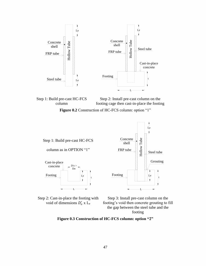
47

Step 1: Build pre-cast HC-FCS

column

Step 2: Install pre-cast column on the

footing cage then cast-in-place the footing

Figure 0.2 Construction of HC-FCS column: option “1”

Step 1: Build pre-cast HC-FCS

column as in OPTION “1”

Step 2: Cast-in-place the footing with

void of dimensions 𝐷𝑜′ x Le

Step 3: Install pre-cast column on the

footing’s void then concrete grouting to fill

the gap between the steel tube and the

footing

Figure 0.3 Construction of HC-FCS column: option “2”

Holl

ow

TubeConcrete

shell

FRP tube

Steel tube Le

Le

Footing

L

Holl

ow

Tube

FRP tubeSteel tube

Le

Cast-in-placeconcrete

t

Concreteshell

Footing

L

tLe

Holl

ow

TubeConcrete

shell

FRP tube

Le

Grouting

Steel tube

Footing

L

D'o >Do

Le t

Cast-in-placeconcrete

48

3.3 Construction Sequence of the Investigated Columns

The construction sequence of the four columns is presented as following:

Prepare reinforcement cages of the footings and the RC-column

(a) (b)

Figure 0.4 Preparing reinforcement cages: (a) footing, (b) RC-column

Install reinforcement cages into the formwork

(a) (b)

Figure 0.5 Install reinforcement cages into formwork: (a) footing, (b) RC-column

49

Install steel tube into footing

The embedded length (Le) of the steel tube into the footing, measuring from the top of

footing to the bottom of the steel tube into the footing, was 25 inches, which was approximately 1.6

times the diameter of the steel tube (Di).

(a) (b) (c)

Figure 0.6 Install the steel tube into the footing: (a) moving the steel tube, (b) putting the steel tube

into the footing, (c) and verticality check of the steel tube

Concrete pouring of the footing

Figure 0.7 Concrete pouring of the footing

50

Install the formwork of the RC-column and the FRP tube for the HC-FCS column

Figure 0.8 Install the formwork of the RC-column and the FRP tube for the HC-FCS column

Concrete pouring of the columns

Figure 0.9 Concrete pouring of the columns

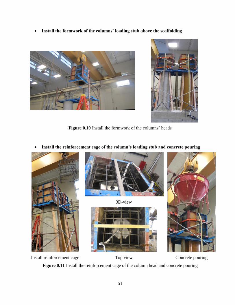
51

Install the formwork of the columns’ loading stub above the scaffolding

Figure 0.10 Install the formwork of the columns’ heads

Install the reinforcement cage of the column’s loading stub and concrete pouring

3D-view

Install reinforcement cage Top view Concrete pouring

Figure 0.11 Install the reinforcement cage of the column head and concrete pouring

52

Paint the concrete surfaces

Figure 0.12 Paint the concrete surfaces

3.4 Instrumentations

3.4.1 Measuring Displacement and Curvature of the Column

Fifteen linear-variable-displacement-transducers (LVDTs) and string potentiometers (SPs)

were employed for the measurement of displacement and curvature of the column. Two more

LVDTs were attached on the footings to measure the rocking and sliding of the footings. The effect

of the rocking and sliding were subtracted from the calculation of displacement and curvature of the

columns. A layout of the LDVTs and SPs is depicted in fig. 3.13. All of the LVDTs and SPs were

attached to a reference column in order to collect the net readings from the LDVDTs and SPs. Four

LVDTs were mounted each on the north and south faces for the curvature measurement at the

plastic end region.

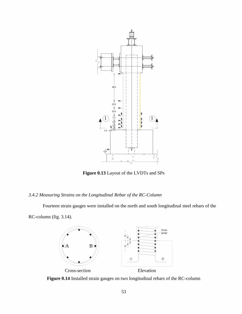
53

Figure 0.13 Layout of the LVDTs and SPs

3.4.2 Measuring Strains on the Longitudinal Rebar of the RC-Column

Fourteen strain gauges were installed on the north and south longitudinal steel rebars of the

RC-column (fig. 3.14).

Cross-section Elevation

Figure 0.14 Installed strain gauges on two longitudinal rebars of the RC-column

3.0

5.0

5.0

7.5

10.0

10.0

38.0

6.0

1.0

1 1

A B

Strain

gauge

48

12

48

12

A B

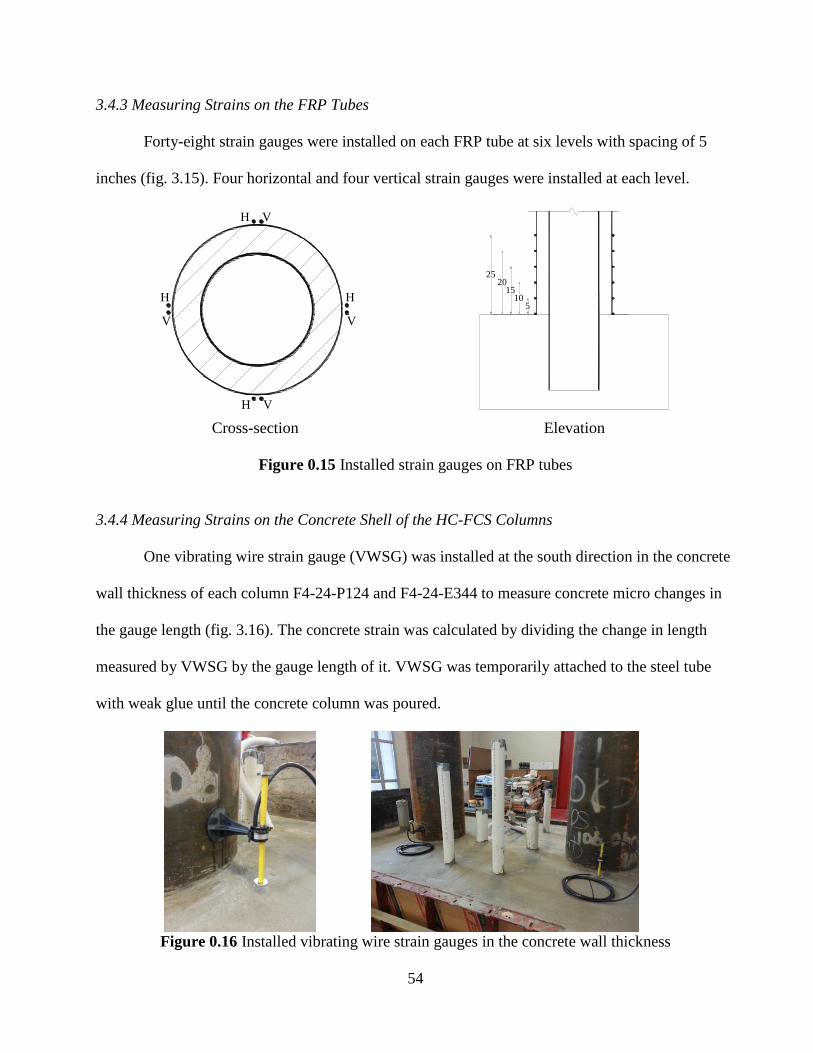
54

3.4.3 Measuring Strains on the FRP Tubes

Forty-eight strain gauges were installed on each FRP tube at six levels with spacing of 5

inches (fig. 3.15). Four horizontal and four vertical strain gauges were installed at each level.

Cross-section Elevation

Figure 0.15 Installed strain gauges on FRP tubes

3.4.4 Measuring Strains on the Concrete Shell of the HC-FCS Columns

One vibrating wire strain gauge (VWSG) was installed at the south direction in the concrete

wall thickness of each column F4-24-P124 and F4-24-E344 to measure concrete micro changes in

the gauge length (fig. 3.16). The concrete strain was calculated by dividing the change in length

measured by VWSG by the gauge length of it. VWSG was temporarily attached to the steel tube

with weak glue until the concrete column was poured.

Figure 0.16 Installed vibrating wire strain gauges in the concrete wall thickness

V

H

V

H

H V

H V

510

1520

25

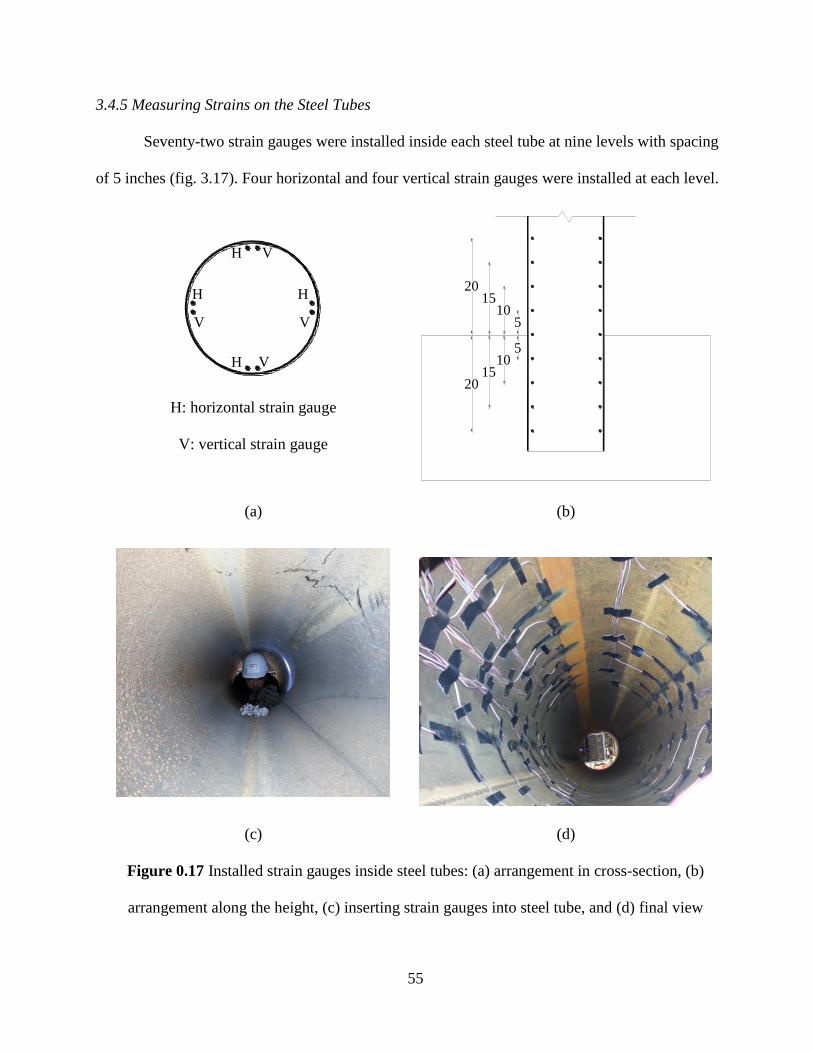
55

3.4.5 Measuring Strains on the Steel Tubes

Seventy-two strain gauges were installed inside each steel tube at nine levels with spacing

of 5 inches (fig. 3.17). Four horizontal and four vertical strain gauges were installed at each level.

H: horizontal strain gauge

V: vertical strain gauge

(a) (b)

(c) (d)

Figure 0.17 Installed strain gauges inside steel tubes: (a) arrangement in cross-section, (b)

arrangement along the height, (c) inserting strain gauges into steel tube, and (d) final view

V

H

H V

V

H

H V

510

1520

510

1520

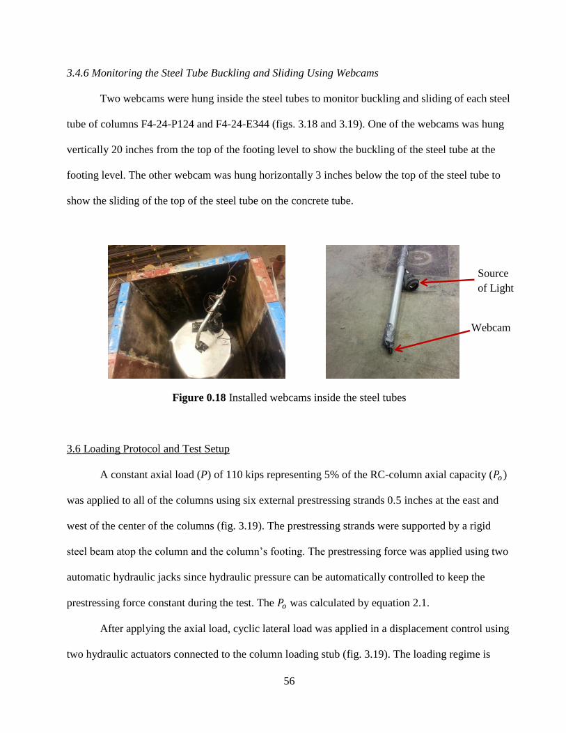
56

3.4.6 Monitoring the Steel Tube Buckling and Sliding Using Webcams

Two webcams were hung inside the steel tubes to monitor buckling and sliding of each steel

tube of columns F4-24-P124 and F4-24-E344 (figs. 3.18 and 3.19). One of the webcams was hung

vertically 20 inches from the top of the footing level to show the buckling of the steel tube at the

footing level. The other webcam was hung horizontally 3 inches below the top of the steel tube to

show the sliding of the top of the steel tube on the concrete tube.

Figure 0.18 Installed webcams inside the steel tubes

3.6 Loading Protocol and Test Setup

A constant axial load (P) of 110 kips representing 5% of the RC-column axial capacity (𝑃𝑜)

was applied to all of the columns using six external prestressing strands 0.5 inches at the east and

west of the center of the columns (fig. 3.19). The prestressing strands were supported by a rigid

steel beam atop the column and the column’s footing. The prestressing force was applied using two

automatic hydraulic jacks since hydraulic pressure can be automatically controlled to keep the

prestressing force constant during the test. The 𝑃𝑜 was calculated by equation 2.1.

After applying the axial load, cyclic lateral load was applied in a displacement control using

two hydraulic actuators connected to the column loading stub (fig. 3.19). The loading regime is

Source

of Light

Webcam

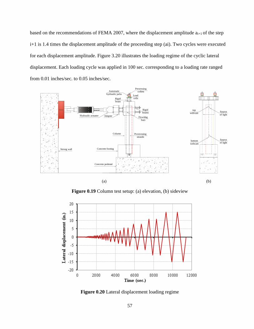
57

based on the recommendations of FEMA 2007, where the displacement amplitude ai+1 of the step

i+1 is 1.4 times the displacement amplitude of the proceeding step (ai). Two cycles were executed

for each displacement amplitude. Figure 3.20 illustrates the loading regime of the cyclic lateral

displacement. Each loading cycle was applied in 100 sec. corresponding to a loading rate ranged

from 0.01 inches/sec. to 0.05 inches/sec.

(a) (b)

Figure 0.19 Column test setup: (a) elevation, (b) sideview

Figure 0.20 Lateral displacement loading regime

Concrete pedestal

Concrete footing

Column

Hydraulic actuator Adapter

Rigid

beam

Load

cells

Automatic

hydraulic jacks

Presressing

collets

Prestressing

strands

Rigid

beams

Dywidag

bars

Strong wall

top

webcam

bottom

webcam

Source

of light

Sourceof light

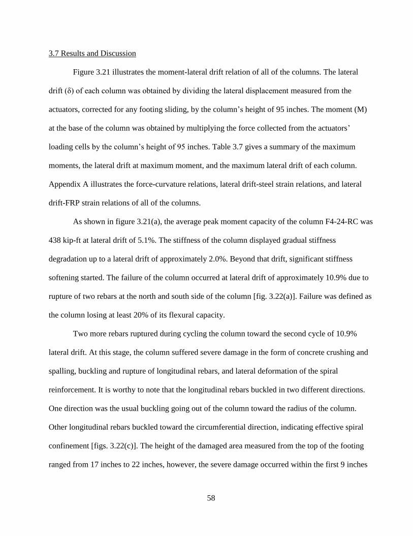
58

3.7 Results and Discussion

Figure 3.21 illustrates the moment-lateral drift relation of all of the columns. The lateral

drift (δ) of each column was obtained by dividing the lateral displacement measured from the

actuators, corrected for any footing sliding, by the column’s height of 95 inches. The moment (M)

at the base of the column was obtained by multiplying the force collected from the actuators’

loading cells by the column’s height of 95 inches. Table 3.7 gives a summary of the maximum

moments, the lateral drift at maximum moment, and the maximum lateral drift of each column.

Appendix A illustrates the force-curvature relations, lateral drift-steel strain relations, and lateral

drift-FRP strain relations of all of the columns.

As shown in figure 3.21(a), the average peak moment capacity of the column F4-24-RC was

438 kip-ft at lateral drift of 5.1%. The stiffness of the column displayed gradual stiffness

degradation up to a lateral drift of approximately 2.0%. Beyond that drift, significant stiffness

softening started. The failure of the column occurred at lateral drift of approximately 10.9% due to

rupture of two rebars at the north and south side of the column [fig. 3.22(a)]. Failure was defined as

the column losing at least 20% of its flexural capacity.

Two more rebars ruptured during cycling the column toward the second cycle of 10.9%

lateral drift. At this stage, the column suffered severe damage in the form of concrete crushing and

spalling, buckling and rupture of longitudinal rebars, and lateral deformation of the spiral

reinforcement. It is worthy to note that the longitudinal rebars buckled in two different directions.

One direction was the usual buckling going out of the column toward the radius of the column.

Other longitudinal rebars buckled toward the circumferential direction, indicating effective spiral

confinement [figs. 3.22(c)]. The height of the damaged area measured from the top of the footing

ranged from 17 inches to 22 inches, however, the severe damage occurred within the first 9 inches

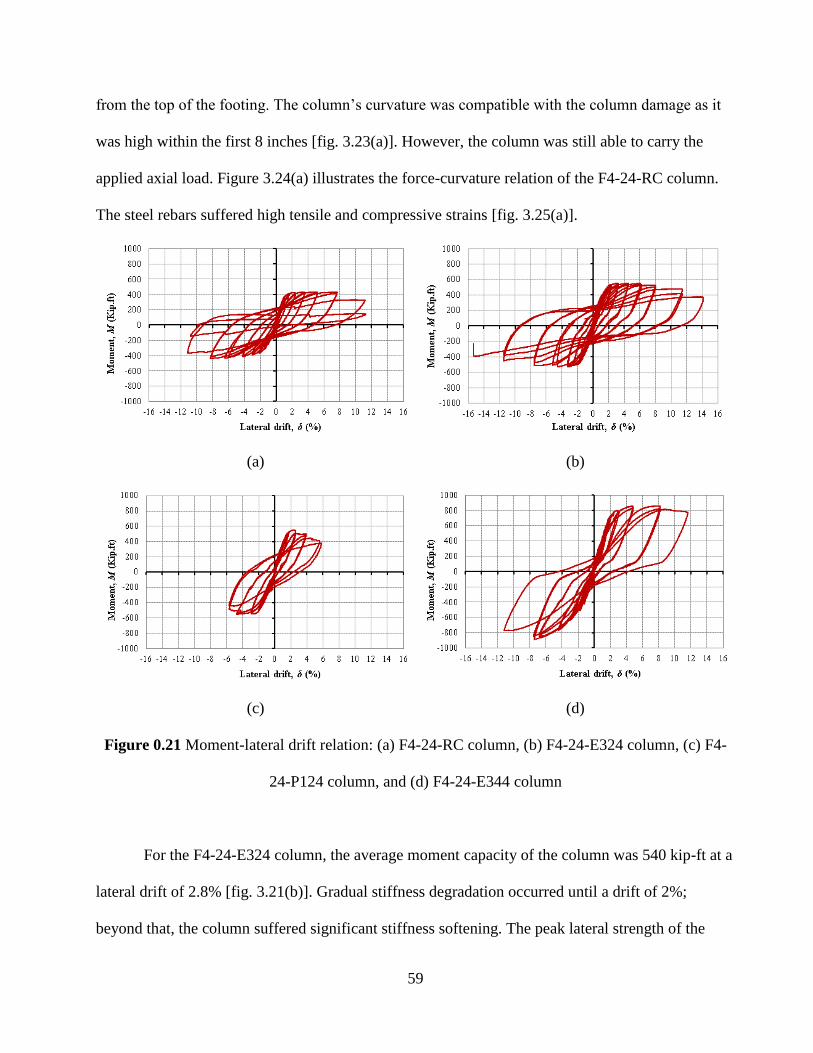
59

from the top of the footing. The column’s curvature was compatible with the column damage as it

was high within the first 8 inches [fig. 3.23(a)]. However, the column was still able to carry the

applied axial load. Figure 3.24(a) illustrates the force-curvature relation of the F4-24-RC column.

The steel rebars suffered high tensile and compressive strains [fig. 3.25(a)].

(a) (b)

(c) (d)

Figure 0.21 Moment-lateral drift relation: (a) F4-24-RC column, (b) F4-24-E324 column, (c) F4-

24-P124 column, and (d) F4-24-E344 column

For the F4-24-E324 column, the average moment capacity of the column was 540 kip-ft at a

lateral drift of 2.8% [fig. 3.21(b)]. Gradual stiffness degradation occurred until a drift of 2%;

beyond that, the column suffered significant stiffness softening. The peak lateral strength of the

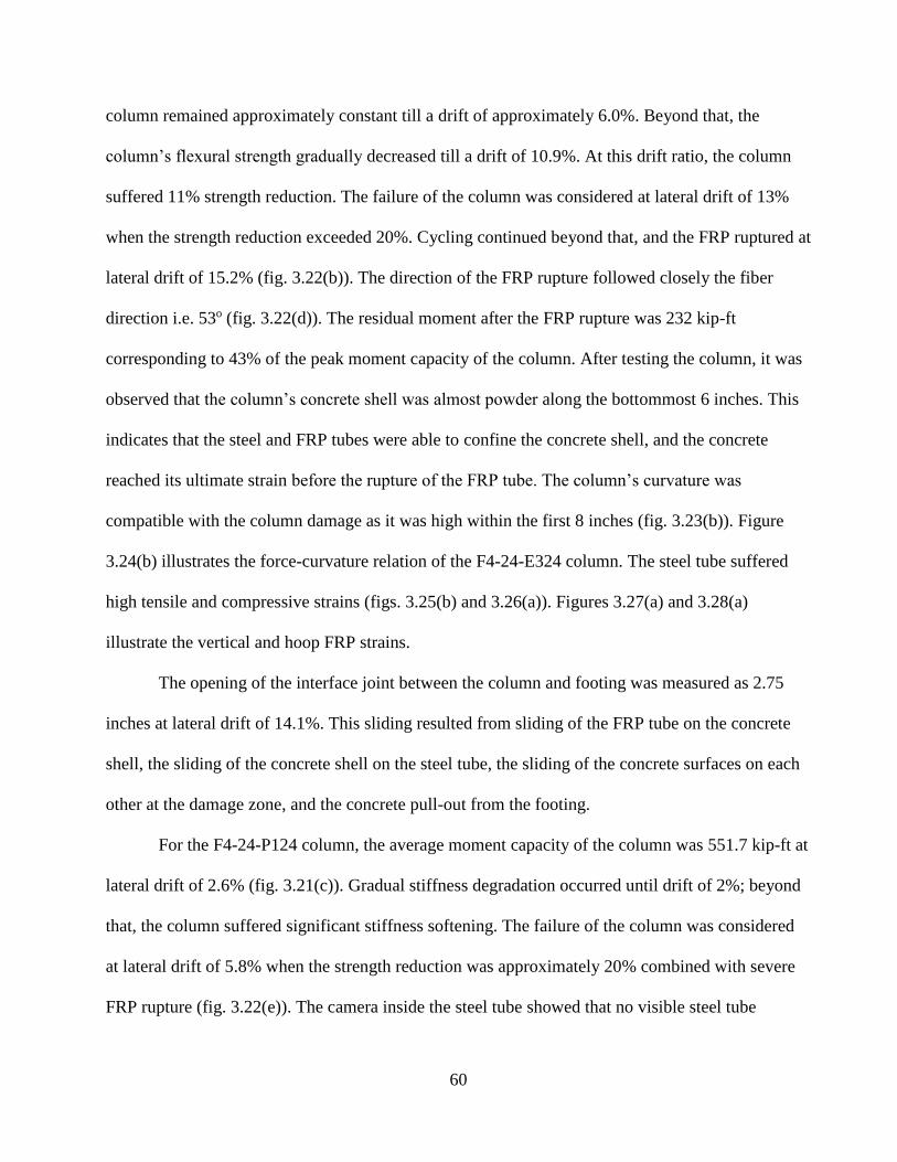
60

column remained approximately constant till a drift of approximately 6.0%. Beyond that, the

column’s flexural strength gradually decreased till a drift of 10.9%. At this drift ratio, the column

suffered 11% strength reduction. The failure of the column was considered at lateral drift of 13%

when the strength reduction exceeded 20%. Cycling continued beyond that, and the FRP ruptured at

lateral drift of 15.2% (fig. 3.22(b)). The direction of the FRP rupture followed closely the fiber

direction i.e. 53o (fig. 3.22(d)). The residual moment after the FRP rupture was 232 kip-ft

corresponding to 43% of the peak moment capacity of the column. After testing the column, it was

observed that the column’s concrete shell was almost powder along the bottommost 6 inches. This

indicates that the steel and FRP tubes were able to confine the concrete shell, and the concrete

reached its ultimate strain before the rupture of the FRP tube. The column’s curvature was

compatible with the column damage as it was high within the first 8 inches (fig. 3.23(b)). Figure

3.24(b) illustrates the force-curvature relation of the F4-24-E324 column. The steel tube suffered

high tensile and compressive strains (figs. 3.25(b) and 3.26(a)). Figures 3.27(a) and 3.28(a)

illustrate the vertical and hoop FRP strains.

The opening of the interface joint between the column and footing was measured as 2.75

inches at lateral drift of 14.1%. This sliding resulted from sliding of the FRP tube on the concrete

shell, the sliding of the concrete shell on the steel tube, the sliding of the concrete surfaces on each

other at the damage zone, and the concrete pull-out from the footing.

For the F4-24-P124 column, the average moment capacity of the column was 551.7 kip-ft at

lateral drift of 2.6% (fig. 3.21(c)). Gradual stiffness degradation occurred until drift of 2%; beyond

that, the column suffered significant stiffness softening. The failure of the column was considered

at lateral drift of 5.8% when the strength reduction was approximately 20% combined with severe

FRP rupture (fig. 3.22(e)). The camera inside the steel tube showed that no visible steel tube

61

buckling was noted. Figure 3.23(c) illustrates that the high column’s curvature was within the first

8 inches from the top of the footing. Figure 3.24(c) illustrates the force-curvature relation of the F4-

24-P124 column. The steel tube suffered high tensile and compressive strains (figs. 3.25(c) and

3.26(b)). Figures 3.27(b) and 3.28(b) illustrate the vertical and hoop FRP strains. Figure 3.29(a)

illustrates the concrete strain-lateral drift relation. The concrete behaved linearly up to the

approximate lateral drift of 1.0%.

For the F4-24-E344 column, the average moment capacity of the column was 874.5 kip-ft at

lateral drift of 7.7% (fig. 3.21(c)). The column suffered significant stiffness softening after the

approximate lateral drift of 8%. The column’s footing suffered severe damage due to the steel tube

pullout (figs. 3.22(f)). The damage indicated that the embedded length of the steel tube was not

enough for that column which explains that the steel tube embedded length is related not only to its

diameter, but it is also related to its thickness. The column lost approximately 15% of its flexural

capacity at lateral drift of 11.6%. Figure 3.23(d) illustrates that the high column’s curvature was

within the first 8 inches from the top of the footing. Figure 3.24(d) illustrates the force-curvature

relation of the F4-24-E344 column. The steel tube suffered high tensile and compressive strains

(figs. 3.25(d) and 3.26(c)). Figures 3.27(c) and 3.28(c) illustrate the vertical and hoop FRP strains.

Figure 3.29(b) illustrates the concrete strain-lateral drift relation. The concrete behaved linearly up

to the approximate lateral drift of 1.0%.

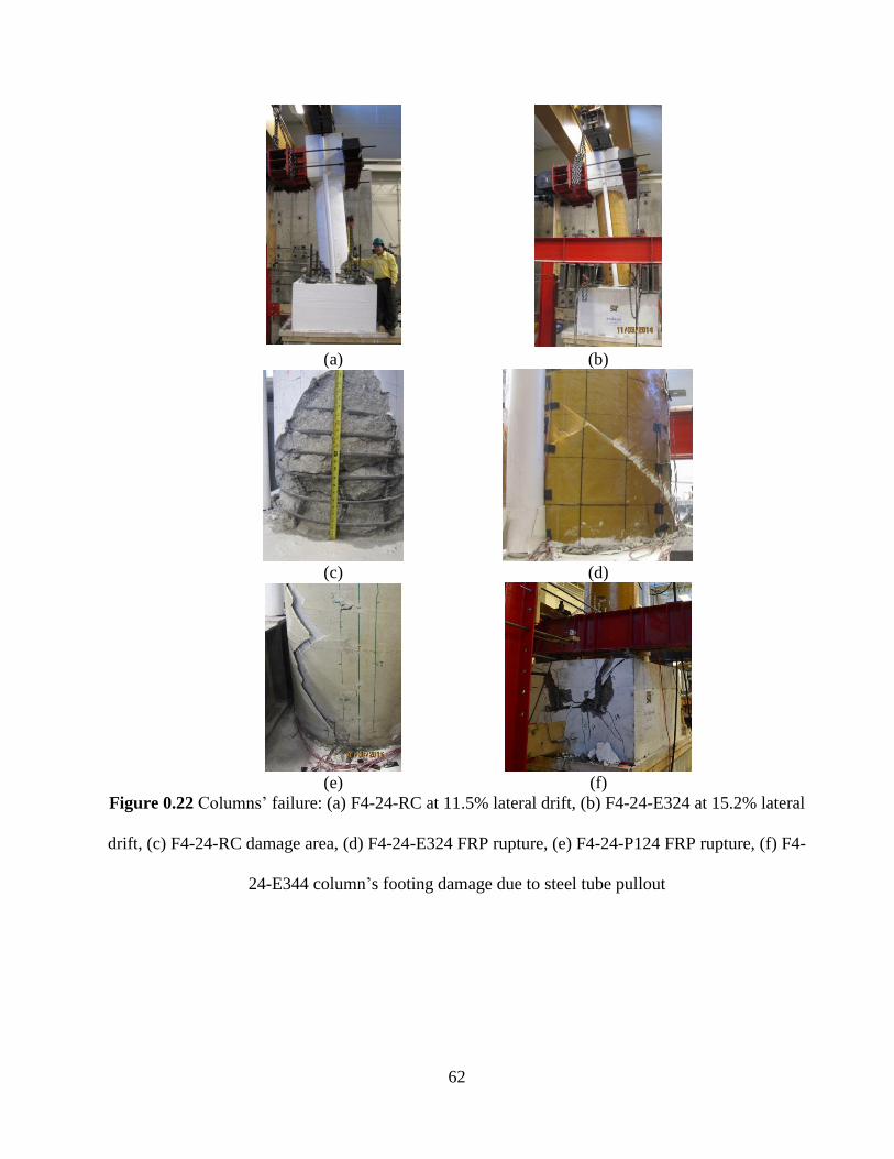
62

(a) (b)

(c) (d)

(e) (f)

Figure 0.22 Columns’ failure: (a) F4-24-RC at 11.5% lateral drift, (b) F4-24-E324 at 15.2% lateral

drift, (c) F4-24-RC damage area, (d) F4-24-E324 FRP rupture, (e) F4-24-P124 FRP rupture, (f) F4-

24-E344 column’s footing damage due to steel tube pullout

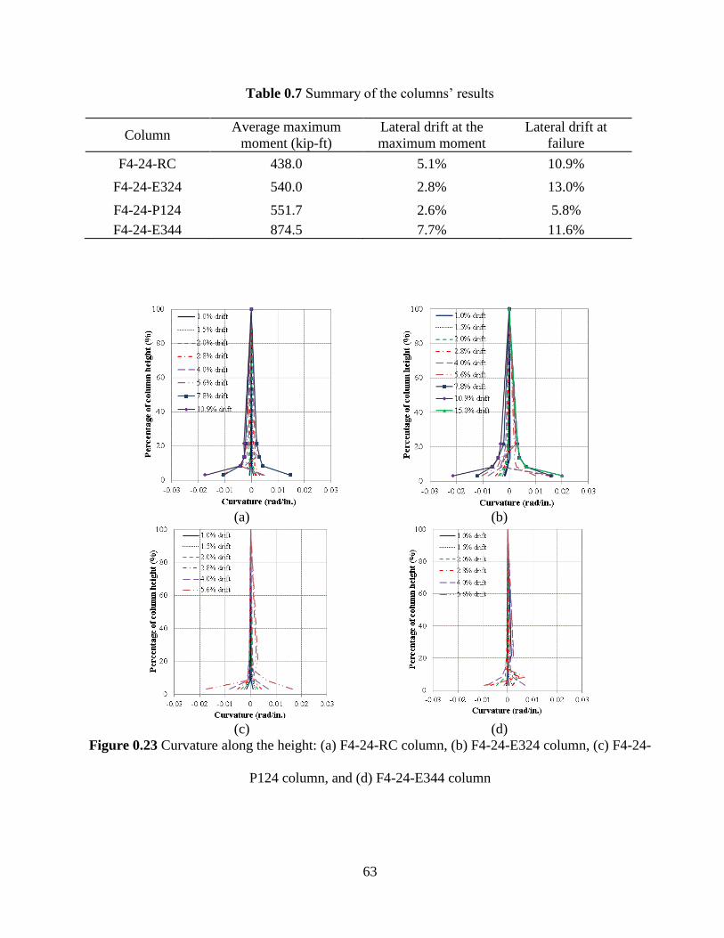
63

Table 0.7 Summary of the columns’ results

Column Average maximum

moment (kip-ft)

Lateral drift at the

maximum moment

Lateral drift at

failure

F4-24-RC 438.0 5.1% 10.9%

F4-24-E324 540.0 2.8% 13.0%

F4-24-P124 551.7 2.6% 5.8%

F4-24-E344 874.5 7.7% 11.6%

(a) (b)

(c) (d)

Figure 0.23 Curvature along the height: (a) F4-24-RC column, (b) F4-24-E324 column, (c) F4-24-

P124 column, and (d) F4-24-E344 column

64

(a) (b)

(c) (d)

Figure 0.24 Force-curvature relation at the level of 3.2% of the column’s height: (a) F4-24-RC

column, (b) F4-24-E324 column, (c) F4-24-P124 column, and (d) F4-24-E344 column

(a) (b)

(c) (d)

Figure 0.25 Lateral drift-vertical steel strain relation for: (a) the F4-24-RC column at 4 inch

from the top of the footing, (b) the F4-24-E324 column at 10 inch from the top of the footing, (c)

the F4-24-P124 column at 10 inch from the top of the footing, and (d) the F4-24-E344 column at 10

inch from the top of the footing

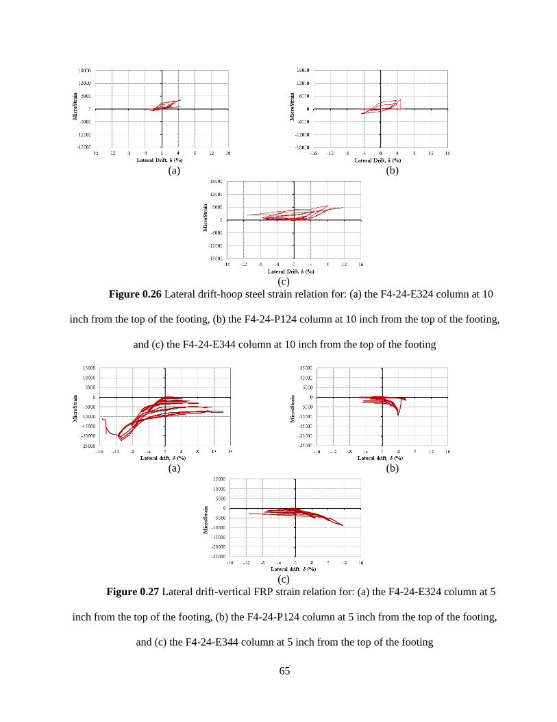
65

(a) (b)

(c)

Figure 0.26 Lateral drift-hoop steel strain relation for: (a) the F4-24-E324 column at 10

inch from the top of the footing, (b) the F4-24-P124 column at 10 inch from the top of the footing,

and (c) the F4-24-E344 column at 10 inch from the top of the footing

(a) (b)

(c)

Figure 0.27 Lateral drift-vertical FRP strain relation for: (a) the F4-24-E324 column at 5

inch from the top of the footing, (b) the F4-24-P124 column at 5 inch from the top of the footing,

and (c) the F4-24-E344 column at 5 inch from the top of the footing

66

(a) (b)

(c)

Figure 0.28 Lateral drift-hoop FRP strain relation for: (a) the F4-24-E324 column at 5 inch

from the top of the footing, (b) the F4-24-P124 column at 5 inch from the top of the footing, and (c)

the F4-24-E344 column at 5 inch from the top of the footing

(a) (b)

Figure 0.29 Lateral drift-concrete strain relation for: (a) the F4-24-P124 column and (b) the

F4-24-E344 column

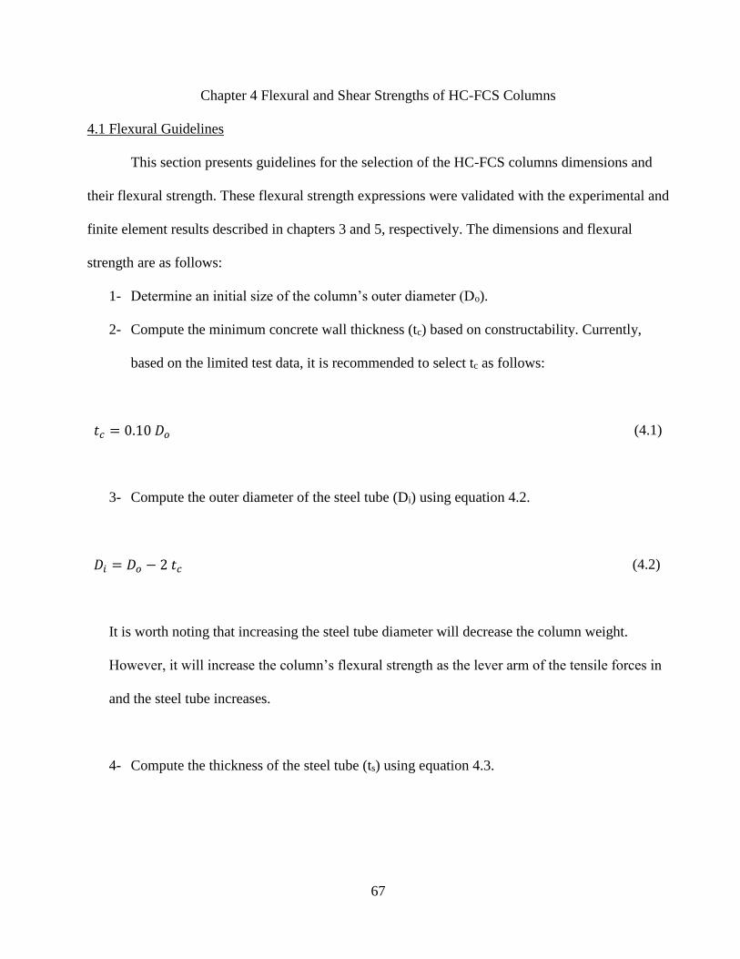
67

Chapter 4 Flexural and Shear Strengths of HC-FCS Columns

4.1 Flexural Guidelines

This section presents guidelines for the selection of the HC-FCS columns dimensions and

their flexural strength. These flexural strength expressions were validated with the experimental and

finite element results described in chapters 3 and 5, respectively. The dimensions and flexural

strength are as follows:

1- Determine an initial size of the column’s outer diameter (Do).

2- Compute the minimum concrete wall thickness (tc) based on constructability. Currently,

based on the limited test data, it is recommended to select tc as follows:

𝑡𝑐 = 0.10 𝐷𝑜 (4.1)

3- Compute the outer diameter of the steel tube (Di) using equation 4.2.

𝐷𝑖 = 𝐷𝑜 − 2 𝑡𝑐 (4.2)

It is worth noting that increasing the steel tube diameter will decrease the column weight.

However, it will increase the column’s flexural strength as the lever arm of the tensile forces in

and the steel tube increases.

4- Compute the thickness of the steel tube (ts) using equation 4.3.

68

𝑡𝑠 =𝐷𝑖

64 (4.3)

The steel tube’s thickness is controlled by the diameter-to-thickness ratio (Di/ts). Thinner steel

tubes are more susceptible to local buckling. However, thicker steel tubes would increase the

column’s weight, cost, and strength. The tubes that were investigated during the current

research have maximum Di/ts of 64. Hence, until further research is available, it is

recommended to keep Di/ts to 64.

5- Compute the FRP tube thickness (tFRP) using equations 4.4 and 4.5 for low and high seismic

regions, respectively.

𝑡𝐹𝑅𝑃 = 0.035 𝐷𝑜 𝑓𝑐

′

𝑓𝑡 (4.4)

𝑡𝐹𝑅𝑃 = 0.105 𝐷𝑜 𝑓𝑐

′

𝑓𝑡 (4.5)

Where ft is the ultimate hoop tensile stress of the FRP tube and 𝑓𝑐′ is the cylindrical unconfined

concrete compressive strength at 28 days. A minimum ft value of 40,000 psi is recommended.

The FRP tube represents the concrete confinement which allows the column to reach higher

lateral drift before failure. The thicknesses of two FRP tubes were investigated during the

course of this study. Both thicknesses were able to display large lateral drifts of 13.0% and

5.8% before rupture. Hence, until further research is carried out, the lateral confinement

pressure used in the test columns were used to develop recommendations for the FRP thickness.

69

6- Compute the column’s flexural strength

Nonlinear analysis, considering Navier-Bernoulli’s assumptions and strains compatibility,

was used to calculate the flexural strength of HC-FCS columns. The main assumptions in the

analysis were as follows: (a) the plane section remained plane both before and after deformation

occurred; (b) there was full composite action between the steel tube and concrete; (c) the stress-

strain relationship of steel was assumed elastic-perfectly plastic; d) the stress-strain relationship of

concrete in the FRP-concrete-steel double skin sections (developed by Yu et al. 2006) was adopted.

Moment-curvature analysis (including the applied axial load effects) was conducted, and the

bending strength was determined for each column.

The concrete compressive strain at the extreme fibers (εc) was initially assumed. Then, the

distance from the neutral axis to the compressive extreme fibers (c) was incrementally increased

until attaining force equilibrium (ΣFx = 0). During the previous step, the compression and tension

sides of the cross-section were divided to 100 horizontal strip segments based on the polar angle of

each side (fig. 4.1). The stresses and forces in compressive confined concrete, steel in compression,

and steel in tension were calculated at each c value. Consequently, the bending moment and the

curvature were computed. The bending moment was computed around the plastic centroid, which is

the center of gravity (C.G.) of the cross-section as it is a symmetrical section. The concrete

compressive strain at the extreme fibers (εc) was incrementally increased up to ultimate strain (εcu;

Yu et al. 2006). The analytical procedure is presented in the following steps:

a- Compute the sectors’ polar angles (𝜃1, 𝜃2& 𝜃3)

𝜃1 =𝛼1

(𝑛) , 𝜃2 =

𝛼2

(𝑛)& 𝜃3 =

𝛼3

(𝑛) (4.6)

where n is the number of strip segments = 100 in this study

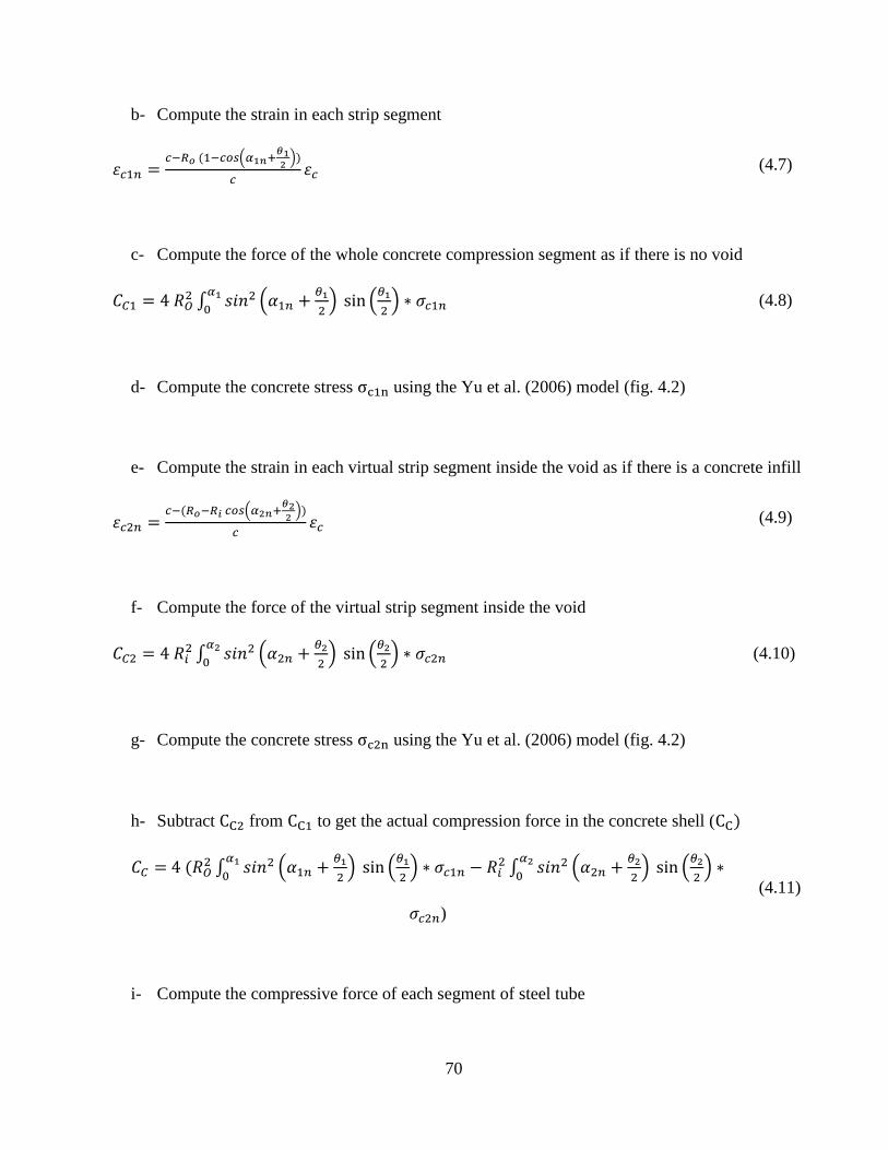
70

b- Compute the strain in each strip segment

휀𝑐1𝑛 =𝑐−𝑅𝑜 (1−𝑐𝑜𝑠(𝛼1𝑛+

𝜃12

))

𝑐휀𝑐 (4.7)

c- Compute the force of the whole concrete compression segment as if there is no void

𝐶𝐶1 = 4 𝑅𝑂2 ∫ 𝑠𝑖𝑛2 (𝛼1𝑛 +

𝜃1

2) sin (

𝜃1

2) ∗ 𝜎𝑐1𝑛

𝛼1

0 (4.8)

d- Compute the concrete stress σc1n using the Yu et al. (2006) model (fig. 4.2)

e- Compute the strain in each virtual strip segment inside the void as if there is a concrete infill

휀𝑐2𝑛 =𝑐−(𝑅𝑜−𝑅𝑖 𝑐𝑜𝑠(𝛼2𝑛+

𝜃22

))

𝑐휀𝑐 (4.9)

f- Compute the force of the virtual strip segment inside the void

𝐶𝐶2 = 4 𝑅𝑖2 ∫ 𝑠𝑖𝑛2 (𝛼2𝑛 +

𝜃2

2) sin (

𝜃2

2) ∗ 𝜎𝑐2𝑛

𝛼2

0 (4.10)

g- Compute the concrete stress σc2n using the Yu et al. (2006) model (fig. 4.2)

h- Subtract CC2 from CC1 to get the actual compression force in the concrete shell (CC)

𝐶𝐶 = 4 (𝑅𝑂2 ∫ 𝑠𝑖𝑛2 (𝛼1𝑛 +

𝜃1

2) sin (

𝜃1

2) ∗ 𝜎𝑐1𝑛

𝛼1

0− 𝑅𝑖

2 ∫ 𝑠𝑖𝑛2 (𝛼2𝑛 +𝜃2

2) sin (

𝜃2

2) ∗

𝛼2

0

𝜎𝑐2𝑛)

(4.11)

i- Compute the compressive force of each segment of steel tube

71

𝐶𝑠𝑐𝑛 = 2 ∫ 𝑡𝑠 ∗ 𝑅𝑖 ∗ 𝜃2

𝑛∗

𝑐−(𝑅𝑜−𝑅𝑖 𝑐𝑜𝑠(𝛼2𝑛+𝜃22

))

𝑐휀𝑐 ∗ 𝐸𝑠

𝛼2

0 (4.12)

where 𝑡𝑠 and 𝐸𝑠 are the thickness and Young’s modulus of the steel tube

j- Compute the tensile force of each segment of steel tube

𝑇𝑠𝑡𝑛 = 2 ∫ 𝑡𝑠 ∗ 𝑅𝑖 ∗ 𝜃3

𝑛∗

(𝑅𝑜 − 𝑐) + 𝑅𝑖 𝑐𝑜𝑠 (𝛼3𝑛 +𝜃3

2 ))

𝑐휀𝑐 ∗ 𝐸𝑠

𝛼3

0

(4.13)

k- After attending the force equilibrium (ΣFx = 0), compute the column’s flexural strength

𝑀𝑛 = ∫ 𝐶𝑐1𝑛 ∗ 𝑅𝑜 ∗ 𝑐𝑜𝑠 (𝛼1𝑛 +𝜃1

2)

𝛼1

0

− ∫ 𝐶𝑐2𝑛 ∗ 𝑅𝑖 ∗ 𝑐𝑜𝑠 (𝛼2𝑛 +𝜃2

2)

𝛼2

0

+ ∫ 𝐶𝑠𝑐𝑛 ∗ 𝑅𝑖 ∗ 𝑐𝑜𝑠 (𝛼2𝑛 +𝜃2

2)

𝛼2

0

+ ∫ 𝑇𝑠𝑡𝑛 ∗ 𝑅𝑖 ∗ 𝑐𝑜𝑠 (𝛼3𝑛 +𝜃3

2)

𝛼3

0

(4.14)

where Mn is the nominal flexural strength of the column

m- Check the column design comparable to the ultimate applied loads

0.9 𝑀𝑛 ≥ 𝑀𝑢 (4.15)

where Mu is the factored applied moment on the column due to external loads

Figure 0.1 Cross-sectional analysis

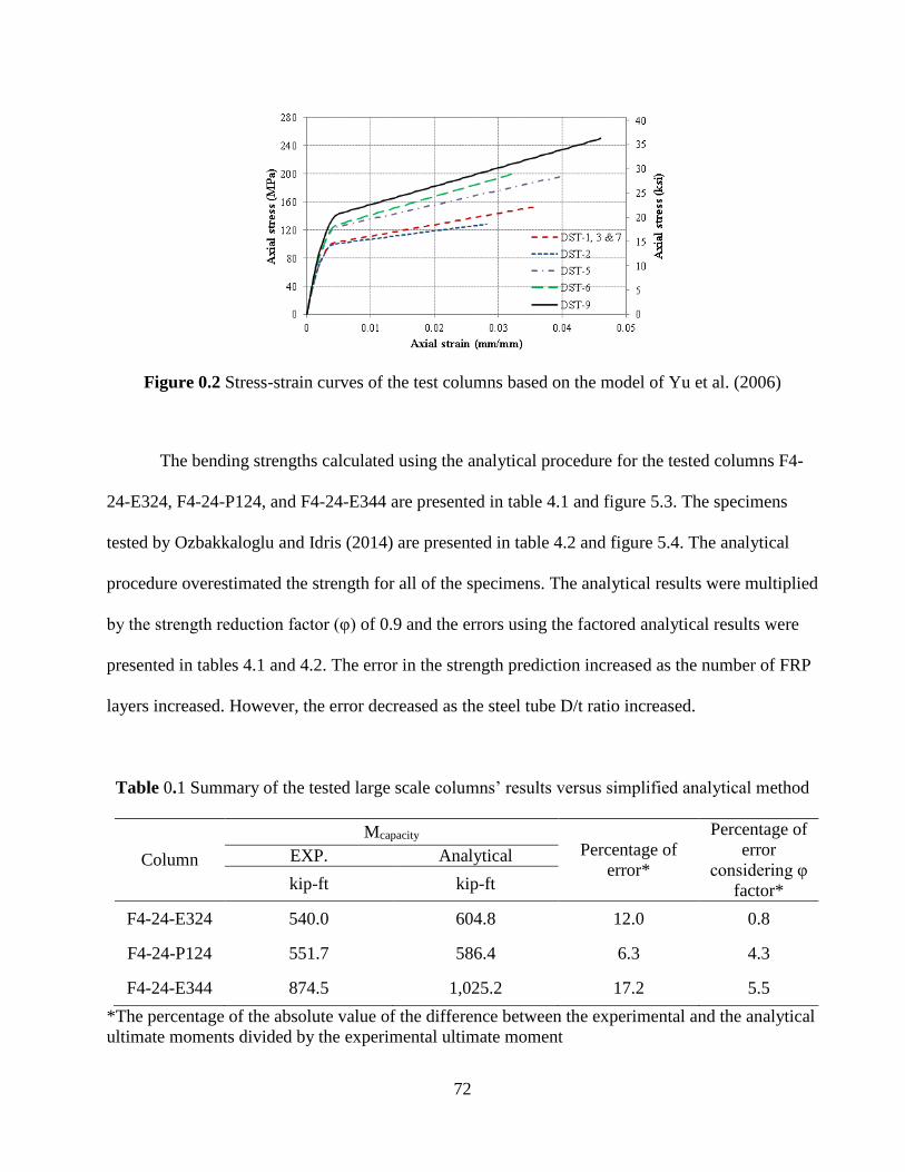
72

Figure 0.2 Stress-strain curves of the test columns based on the model of Yu et al. (2006)

The bending strengths calculated using the analytical procedure for the tested columns F4-

24-E324, F4-24-P124, and F4-24-E344 are presented in table 4.1 and figure 5.3. The specimens

tested by Ozbakkaloglu and Idris (2014) are presented in table 4.2 and figure 5.4. The analytical

procedure overestimated the strength for all of the specimens. The analytical results were multiplied

by the strength reduction factor (φ) of 0.9 and the errors using the factored analytical results were

presented in tables 4.1 and 4.2. The error in the strength prediction increased as the number of FRP

layers increased. However, the error decreased as the steel tube D/t ratio increased.

Table 0.1 Summary of the tested large scale columns’ results versus simplified analytical method

Column

Mcapacity Percentage of

error*

Percentage of

error

considering φ

factor*

EXP. Analytical

kip-ft kip-ft

F4-24-E324 540.0 604.8 12.0 0.8

F4-24-P124 551.7 586.4 6.3 4.3

F4-24-E344 874.5 1,025.2 17.2 5.5

*The percentage of the absolute value of the difference between the experimental and the analytical

ultimate moments divided by the experimental ultimate moment

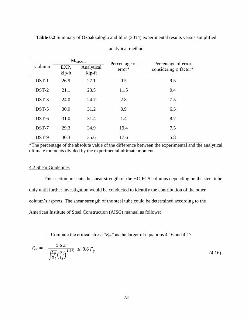
73

Table 0.2 Summary of Ozbakkaloglu and Idris (2014) experimental results versus simplified

analytical method

Column

Mcapacity Percentage of

error*

Percentage of error

considering φ factor* EXP. Analytical

kip-ft kip-ft

DST-1 26.9 27.1 0.5 9.5

DST-2 21.1 23.5 11.5 0.4

DST-3 24.0 24.7 2.8 7.5

DST-5 30.0 31.2 3.9 6.5

DST-6 31.0 31.4 1.4 8.7

DST-7 29.3 34.9 19.4 7.5

DST-9 30.3 35.6 17.6 5.8

*The percentage of the absolute value of the difference between the experimental and the analytical


4.2 Shear Guidelines

This section presents the shear strength of the HC-FCS columns depending on the steel tube

only until further investigation would be conducted to identify the contribution of the other

column’s aspects. The shear strength of the steel tube could be determined according to the

American Institute of Steel Construction (AISC) manual as follows:

a- Compute the critical stress “𝐹𝑐𝑟” as the larger of equations 4.16 and 4.17

𝐹𝑐𝑟 =

1.6 𝐸

√𝐿𝑣𝐷𝑖

(𝐷𝑖𝑡𝑠

)1.25 ≤ 0.6 𝐹𝑦

(4.16)

74

𝐹𝑐𝑟 =

0.78 𝐸

(𝐷𝑖𝑡𝑠

)1.5 ≤ 0.6 𝐹𝑦

(4.17)

Where E = Young’s modulus of steel = 29,000 ksi, Lv = half the span of the steel tube, Fy = the

yield stress of the steel tube, Di = the outer diameter of the steel tube, and ts = the steel tube

thickness

b- Compute the shear capacity of the steel tube “Vn” using equation 4.18

𝑉𝑛 =1

2 (𝜋 𝐷𝑖 𝑡𝑠) 𝐹𝑐𝑟 (4.18)

c- Check the shear capacity comparable to the factored shear demand “Vu” using equation

4.19

0.9 𝑉𝑛 ≥ 𝑉𝑢 (4.19)

75

Chapter 5 Finite Element Modeling

This chapter describes the finite element modeling of HC-FCS’s behavior under a constant

axial compression load and lateral pushover. The LS-DYNA software was used to design and

verify the models against the experimental results gathered from seven HC-FCS columns tested by

Ozbakkaloglu and Idris (2014). These columns had a concrete compressive strength (fc′) that was

between 13,775 psi and 18,850 psi. Either aramid (AFRP) or carbon (CFRP) was used to

manufacture the FRP tubes (see Table 5.1). The columns were tested under axial loads (P) between

92.2 kips and 155.1 kips. These loads were corresponding to 0.34 to 0.45 of the columns nominal

axial capacity (Po) where Po was calculated by eqn. (2.1).

Table 0.1 Summary of columns variables (reproduced after Ozbakkaloglu and Idris 2014)

Column 𝑓𝑐

′ FRP tube Inner steel tube P P/Po

(psi) Material n* t (inch) (kips)

DST-1 13,775 AFRP 3 0.126 122.5 0.45

DST-2 13,775 AFRP 2 0.126 92.2 0.34

DST-3 13,775 AFRP 3 0.126 92.2 0.34

DST-5 16,675 AFRP 4 0.126 140.5 0.45

DST-6 16,675 CFRP 5 0.126 140.5 0.45

DST-7 13,775 AFRP 3 0.217 151.7 0.45

DST-9 18,850 AFRP 6 0.126 155.1 0.45

*n: number of FRP layers

These models were next used to conduct a parametric study investigating the effects of the

applied axial load level, concrete strength, concrete wall thickness, the steel tube’s diameter-to-

thickness ratio (D/t), and the number of FRP layers on the HC-FCS column’s behavior. Analytical

models will be presented later in chapter 4 to predict the column’s flexural strength.

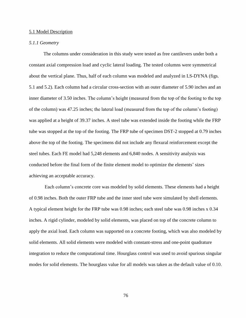
76

5.1 Model Description

5.1.1 Geometry

The columns under consideration in this study were tested as free cantilevers under both a

constant axial compression load and cyclic lateral loading. The tested columns were symmetrical

about the vertical plane. Thus, half of each column was modeled and analyzed in LS-DYNA (figs.

5.1 and 5.2). Each column had a circular cross-section with an outer diameter of 5.90 inches and an

inner diameter of 3.50 inches. The column’s height (measured from the top of the footing to the top

of the column) was 47.25 inches; the lateral load (measured from the top of the column’s footing)

was applied at a height of 39.37 inches. A steel tube was extended inside the footing while the FRP

tube was stopped at the top of the footing. The FRP tube of specimen DST-2 stopped at 0.79 inches

above the top of the footing. The specimens did not include any flexural reinforcement except the

steel tubes. Each FE model had 5,248 elements and 6,840 nodes. A sensitivity analysis was

conducted before the final form of the finite element model to optimize the elements’ sizes

achieving an acceptable accuracy.

Each column’s concrete core was modeled by solid elements. These elements had a height

of 0.98 inches. Both the outer FRP tube and the inner steel tube were simulated by shell elements.

A typical element height for the FRP tube was 0.98 inches; each steel tube was 0.98 inches x 0.34

inches. A rigid cylinder, modeled by solid elements, was placed on top of the concrete column to

apply the axial load. Each column was supported on a concrete footing, which was also modeled by

solid elements. All solid elements were modeled with constant-stress and one-point quadrature

integration to reduce the computational time. Hourglass control was used to avoid spurious singular

modes for solid elements. The hourglass value for all models was taken as the default value of 0.10.

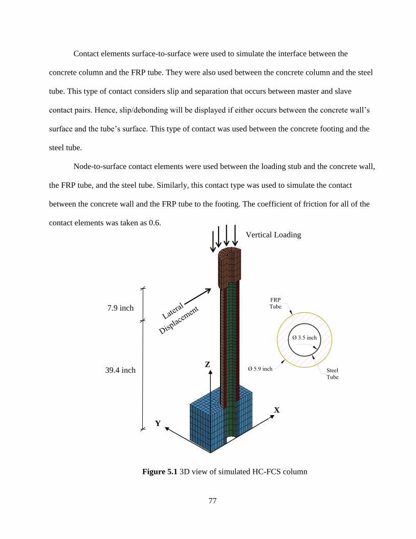
77

Contact elements surface-to-surface were used to simulate the interface between the

concrete column and the FRP tube. They were also used between the concrete column and the steel

tube. This type of contact considers slip and separation that occurs between master and slave

contact pairs. Hence, slip/debonding will be displayed if either occurs between the concrete wall’s

surface and the tube’s surface. This type of contact was used between the concrete footing and the

steel tube.

Node-to-surface contact elements were used between the loading stub and the concrete wall,

the FRP tube, and the steel tube. Similarly, this contact type was used to simulate the contact

between the concrete wall and the FRP tube to the footing. The coefficient of friction for all of the

contact elements was taken as 0.6.

Figure 5.1 3D view of simulated HC-FCS column

Vertical Loading

X

Z

Y

39.4 inch

7.9 inch

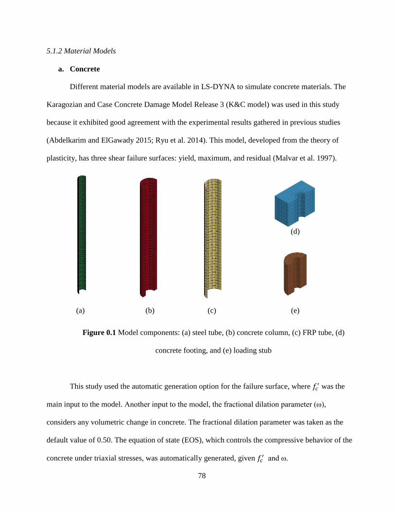
78

5.1.2 Material Models

a. Concrete

Different material models are available in LS-DYNA to simulate concrete materials. The

Karagozian and Case Concrete Damage Model Release 3 (K&C model) was used in this study

because it exhibited good agreement with the experimental results gathered in previous studies

(Abdelkarim and ElGawady 2015; Ryu et al. 2014). This model, developed from the theory of

plasticity, has three shear failure surfaces: yield, maximum, and residual (Malvar et al. 1997).

(d)

(a) (b) (c) (e)

Figure 0.1 Model components: (a) steel tube, (b) concrete column, (c) FRP tube, (d)

concrete footing, and (e) loading stub

This study used the automatic generation option for the failure surface, where 𝑓𝑐′ was the

main input to the model. Another input to the model, the fractional dilation parameter (ω),

considers any volumetric change in concrete. The fractional dilation parameter was taken as the

default value of 0.50. The equation of state (EOS), which controls the compressive behavior of the

concrete under triaxial stresses, was automatically generated, given 𝑓𝑐′ and ω.

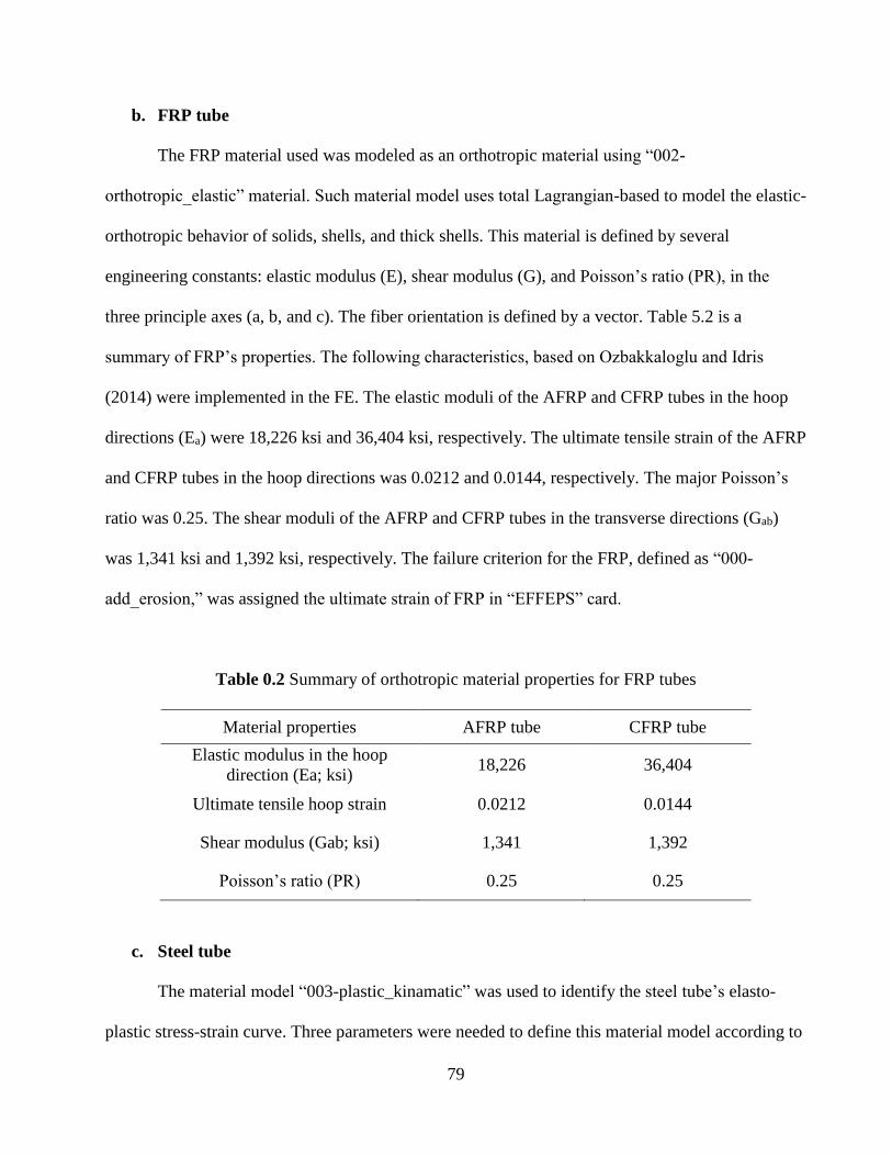
79

b. FRP tube

The FRP material used was modeled as an orthotropic material using “002-

orthotropic_elastic” material. Such material model uses total Lagrangian-based to model the elastic-

orthotropic behavior of solids, shells, and thick shells. This material is defined by several

engineering constants: elastic modulus (E), shear modulus (G), and Poisson’s ratio (PR), in the

three principle axes (a, b, and c). The fiber orientation is defined by a vector. Table 5.2 is a

summary of FRP’s properties. The following characteristics, based on Ozbakkaloglu and Idris

(2014) were implemented in the FE. The elastic moduli of the AFRP and CFRP tubes in the hoop

directions (Ea) were 18,226 ksi and 36,404 ksi, respectively. The ultimate tensile strain of the AFRP

and CFRP tubes in the hoop directions was 0.0212 and 0.0144, respectively. The major Poisson’s

ratio was 0.25. The shear moduli of the AFRP and CFRP tubes in the transverse directions (Gab)

was 1,341 ksi and 1,392 ksi, respectively. The failure criterion for the FRP, defined as “000-

add_erosion,” was assigned the ultimate strain of FRP in “EFFEPS” card.

Table 0.2 Summary of orthotropic material properties for FRP tubes

Material properties AFRP tube CFRP tube

Elastic modulus in the hoop

direction (Ea; ksi) 18,226 36,404

Ultimate tensile hoop strain 0.0212 0.0144

Shear modulus (Gab; ksi) 1,341 1,392

Poisson’s ratio (PR) 0.25 0.25

c. Steel tube

The material model “003-plastic_kinamatic” was used to identify the steel tube’s elasto-

plastic stress-strain curve. Three parameters were needed to define this material model according to

80

the material’s properties: the elastic modulus (E), the yield stress (SIGY), and Poisson’s ratio (PR).

The elastic modulus and the yield stress were 29,725 ksi and 50,750 psi, respectively, for all

columns except DST-7. A different steel tube with a different thickness was used in this column.

Thus, its elastic modulus and yield stress were different: 29,906 ksi and 59,813 psi, respectively.

5.1.3 Boundary Conditions and Loading

Displacement in the Y direction and rotations about both the X and Z axes at the plane of

symmetry were restrained. Displacements and rotations in all directions at the nodes of the

footing’s bottom were prevented.

The loading was applied in two different steps. An axial compressive load was applied to

the top of the loading stub during the first step. These loads were half of those listed in table 5.1 due

to symmetry. During the second step, lateral displacement was applied at the middle nodes of the

common surface, between the column and the loading stub, until failure occurred due to rupture of

the FRP tube or compression failure.

5.2 Results and Discussions

The lateral drift of each of the tested large scale columns was obtained by dividing the

lateral displacement, measured at 95 inches above the footing top, by 95 inches. The moment at the

base of the column was also obtained from FE analysis. The sum of the reactions at the footing

level was multiplied by a column height of 95 inches. The moment versus drift of the tested large

scale columns (obtained from FE analyses) is plotted in fig. 5.3. This figure also depicts the

experimental drift versus the moment for each column. Table 5.3 includes a summary of the finite

element results versus the experimental results for all columns. This table also includes the error in

predicting the ultimate moment of each test specimen. This error was calculated as the absolute

value of the difference between the experimental and the FE ultimate moments divided by the

81

experimental ultimate moment. The error was between 9.5% and 25.1%. All simulated columns

behaved in a manner similar to the tested columns up to failure.

The lateral drift of each of Ozbakkaloglu’s columns was obtained by dividing the lateral

displacement, measured at 39.37 inches above the footing top, by 39.37 inches. The moment at the

base of the column was also obtained from FE analysis; the sum of the reactions at the footing time

was multiplied by a column height of 39.37 inches. The moment versus drift (obtained from FE

analyses) is plotted in fig. 5.4. This figure also depicts the experimental drift versus the moment for

each column. Table 5.4 includes a summary of the finite element results versus the experimental

results for all columns. This table also includes the error in predicting the ultimate moment of each

test specimen. This error was calculated as the absolute value of the difference between the

experimental and the FE ultimate moments divided by the experimental ultimate moment. The error

was between 1.3% and 8.9%. All simulated columns behaved in a manner similar to the tested

columns up to failure.

Overall, the FE models were able to capture the test specimen’s behavior (fig. 5.4). Column

DST-1 reached peak bending strengths of 26.9 kip-ft and 24.9 kip-ft during the experimental work

and the FE analysis, respectively (fig. 5.4a). The difference between the experimental strength and

the FE strength was 7.4%. The column reached its peak strength at drifts of 5.8% and 5.7% during

the experimental and FE analyses, respectively. However, during the experimental work and

beyond a drift of 6.0%, the column failed abruptly when the FRP tube ruptured. This column failed

due to compression failure that occurred during the FE analysis at a lateral drift of 8.9%.

The FE predicted the initial stiffness until a drift of 1.0% (see fig. 5.4a). At that drift, both

the experimental and the FE analysis revealed a significant nonlinear behavior up to failure. The FE

analysis revealed that the nonlinear behavior began when the concrete column began to uplift at the

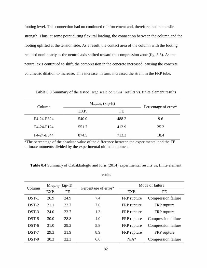
82

footing level. This connection had no continued reinforcement and, therefore, had no tensile

strength. Thus, at some point during flexural loading, the connection between the column and the

footing uplifted at the tension side. As a result, the contact area of the column with the footing

reduced nonlinearly as the neutral axis shifted toward the compression zone (fig. 5.5). As the

neutral axis continued to shift, the compression in the concrete increased, causing the concrete

volumetric dilation to increase. This increase, in turn, increased the strain in the FRP tube.

Table 0.3 Summary of the tested large scale columns’ results vs. finite element results

Column Mcapacity (kip-ft)

Percentage of error* EXP. FE

F4-24-E324 540.0 488.2 9.6

F4-24-P124 551.7 412.9 25.2

F4-24-E344 874.5 713.3 18.4

*The percentage of the absolute value of the difference between the experimental and the FE


Table 0.4 Summary of Ozbakkaloglu and Idris (2014) experimental results vs. finite element

results

Column Mcapacity (kip-ft)

Percentage of error* Mode of failure

EXP. FE EXP. FE

DST-1 26.9 24.9 7.4 FRP rupture Compression failure

DST-2 21.1 22.7 7.6 FRP rupture FRP rupture





DST-9 30.3 32.3 6.6 N/A* Compression failure

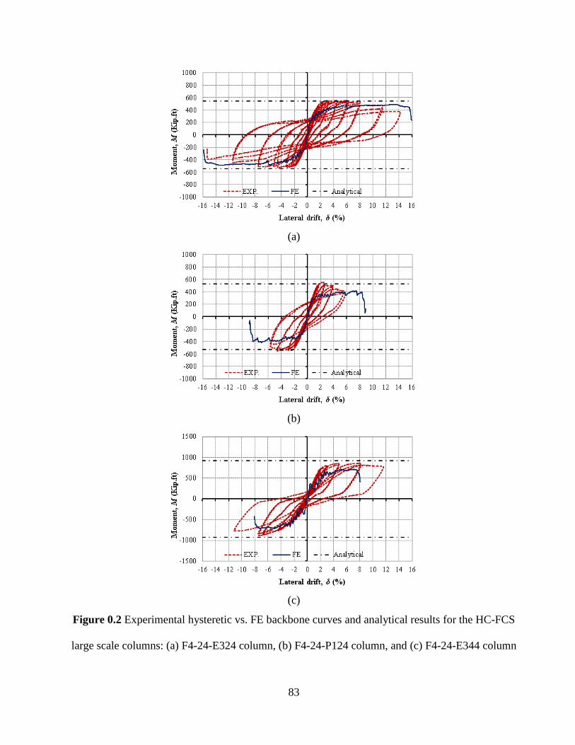
83

(a)

(b)

(c)

Figure 0.2 Experimental hysteretic vs. FE backbone curves and analytical results for the HC-FCS

large scale columns: (a) F4-24-E324 column, (b) F4-24-P124 column, and (c) F4-24-E344 column

84

(a) (b)

(c) (d)

(e) (f)

(g)

Figure 0.3 Experimental (Ozbakkaloglu and Idris 2014 ©ASCE) vs. FE backbone curves for

specimens: (a) DST-1, (b) DST-2, (c) DST-3, (d) DST-5, (e) DST-6, (f) DST-7, and (g) DST-9

85

Figure 0.4 Moving of neutral axis (N.A.) under lateral loading (hatched area is the compression

side)

The FE analysis revealed a confined concrete compressive strength (𝑓𝑐𝑐′ ) of 25,810 psi just

before failure (fig. 5.6). This value indicates that the concrete’s strength increased 87%, signaling

good confinement. Yu et al. (2010) developed a confinement model for HC-FCS. For the given

cross-section, this model predicted an 𝑓𝑐𝑐′ that was equal to 23,235 psi, a value close to the 𝑓𝑐𝑐

′

observed during the FE analysis.

Figure 0.5 Maximum confined concrete stress of the column DST-1 in GPa. (1 GPa = 145 ksi)

N.A.

N.A.

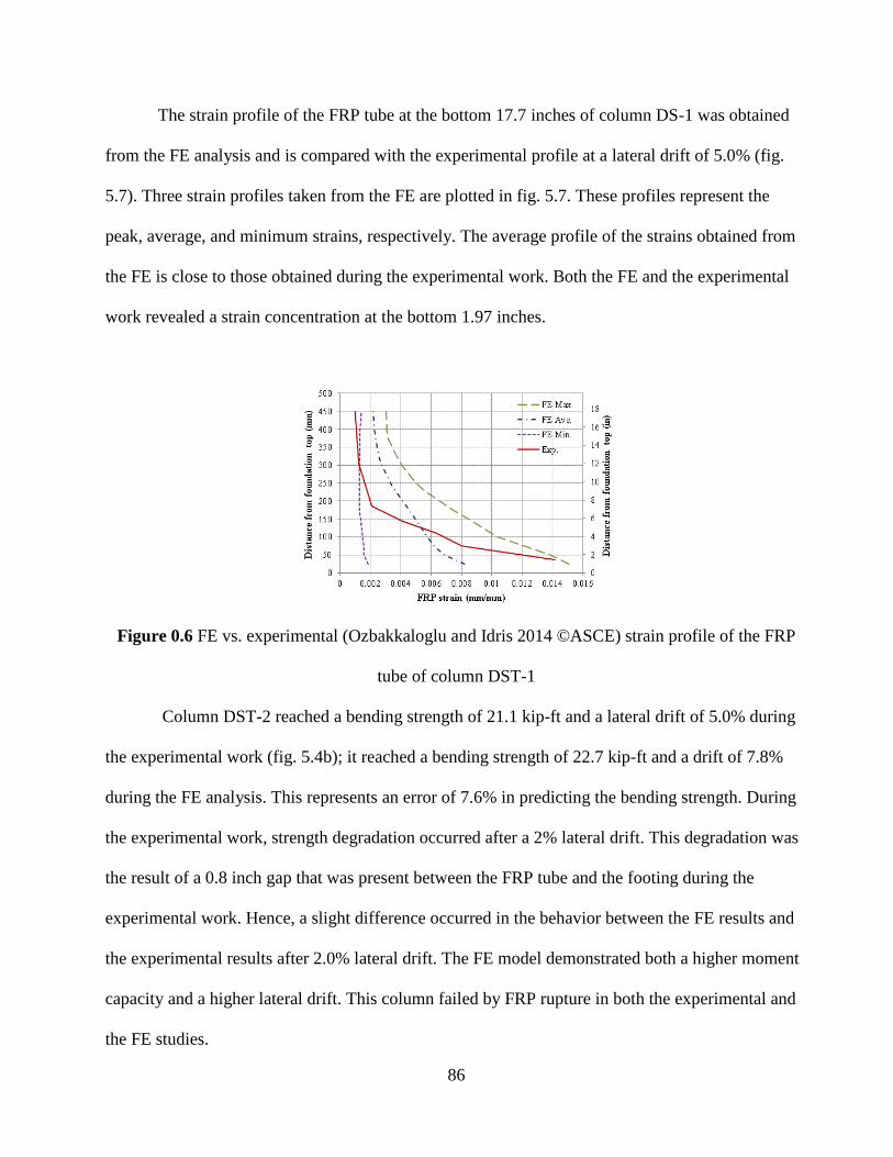
86

The strain profile of the FRP tube at the bottom 17.7 inches of column DS-1 was obtained

from the FE analysis and is compared with the experimental profile at a lateral drift of 5.0% (fig.

5.7). Three strain profiles taken from the FE are plotted in fig. 5.7. These profiles represent the

peak, average, and minimum strains, respectively. The average profile of the strains obtained from

the FE is close to those obtained during the experimental work. Both the FE and the experimental

work revealed a strain concentration at the bottom 1.97 inches.

Figure 0.6 FE vs. experimental (Ozbakkaloglu and Idris 2014 ©ASCE) strain profile of the FRP

tube of column DST-1

Column DST-2 reached a bending strength of 21.1 kip-ft and a lateral drift of 5.0% during

the experimental work (fig. 5.4b); it reached a bending strength of 22.7 kip-ft and a drift of 7.8%

during the FE analysis. This represents an error of 7.6% in predicting the bending strength. During

the experimental work, strength degradation occurred after a 2% lateral drift. This degradation was

the result of a 0.8 inch gap that was present between the FRP tube and the footing during the

experimental work. Hence, a slight difference occurred in the behavior between the FE results and

the experimental results after 2.0% lateral drift. The FE model demonstrated both a higher moment

capacity and a higher lateral drift. This column failed by FRP rupture in both the experimental and

the FE studies.

87

Column DST-3 reached bending strengths of 24.0 kip-ft and 23.7 kip-ft during the

experimental work and the FE analysis (fig. 5.4c), respectively. These values correspond to an error

of 1.3%. Both the FE and the experimental analysis revealed that failure occurred when the FRP

ruptured. The FE analysis predicted the column’s behavior accurately up to a drift of 9.0%. Beyond

that level, the FE analysis exhibited slow strength degradation while the experimental work

presented a nearly constant strength. Degradation in the bending strength during FE analysis

occurred as a result of local buckling in the steel tube.

Columns DST-5 and DST-6 failed during the experimental work at bending strengths of

30.0 kip-ft and 31.0 kip-ft, respectively (figs. 5.4(d) and 5.4(e)). The FE analyses of both columns

predicted peak bending loads of 28.8 kip-ft and 29.2 kip-ft, respectively. This corresponds to errors

of 4.0% and 5.8% for the columns DST-5 and DST-6, respectively. However, while the

experimental work showed that these columns failed at drifts of 6.0% and 7.0% for DST-5 and

DST-6, respectively, the FE analyses showed that these columns failed at drifts of 9.4% and 9.7%.

Both columns failed numerically as a result of compression failure at a confined concrete strength

of 26,100 psi.

During FE analysis, local buckling in the steel tube occurred at a lateral drift of 5.7%.

Hence, the concrete stresses increased considerably because of the significant reduction in the

participation of the steel tube to bending resistance. The experimental work revealed a strength

reduction, likely due to steel buckling, at a drift of 5.0%. The FRP also ruptured, however, after the

steel buckled.

Column DST-7 reached a bending strength of 29.3 kip-ft during the experimental work. The

FE analysis results were in close agreement with the experimental results; the column reached a

bending strength of 31.9 kip-ft (fig. 5.4f), corresponding to an error of 8.9%. The FE analysis and

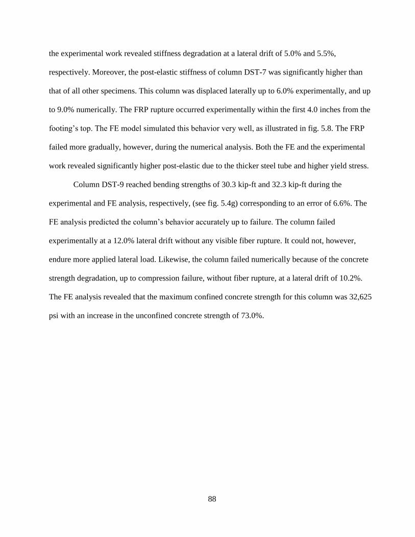
88

the experimental work revealed stiffness degradation at a lateral drift of 5.0% and 5.5%,

respectively. Moreover, the post-elastic stiffness of column DST-7 was significantly higher than

that of all other specimens. This column was displaced laterally up to 6.0% experimentally, and up

to 9.0% numerically. The FRP rupture occurred experimentally within the first 4.0 inches from the

footing’s top. The FE model simulated this behavior very well, as illustrated in fig. 5.8. The FRP

failed more gradually, however, during the numerical analysis. Both the FE and the experimental

work revealed significantly higher post-elastic due to the thicker steel tube and higher yield stress.

Column DST-9 reached bending strengths of 30.3 kip-ft and 32.3 kip-ft during the

experimental and FE analysis, respectively, (see fig. 5.4g) corresponding to an error of 6.6%. The

FE analysis predicted the column’s behavior accurately up to failure. The column failed

experimentally at a 12.0% lateral drift without any visible fiber rupture. It could not, however,

endure more applied lateral load. Likewise, the column failed numerically because of the concrete

strength degradation, up to compression failure, without fiber rupture, at a lateral drift of 10.2%.

The FE analysis revealed that the maximum confined concrete strength for this column was 32,625

psi with an increase in the unconfined concrete strength of 73.0%.

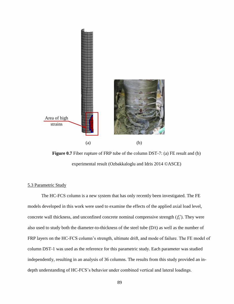
89

(a) (b)

Figure 0.7 Fiber rupture of FRP tube of the column DST-7: (a) FE result and (b)

experimental result (Ozbakkaloglu and Idris 2014 ©ASCE)

5.3 Parametric Study

The HC-FCS column is a new system that has only recently been investigated. The FE

models developed in this work were used to examine the effects of the applied axial load level,

concrete wall thickness, and unconfined concrete nominal compressive strength (𝑓𝑐′). They were

also used to study both the diameter-to-thickness of the steel tube (D/t) as well as the number of

FRP layers on the HC-FCS column’s strength, ultimate drift, and mode of failure. The FE model of

column DST-1 was used as the reference for this parametric study. Each parameter was studied

independently, resulting in an analysis of 36 columns. The results from this study provided an in-

depth understanding of HC-FCS’s behavior under combined vertical and lateral loadings.

Area of high

strains

90

The columns’ overall behavior was as follows. Steel tubes yielded under tension and

compression. This yielding was followed by an onset of local buckling at the section just above the

concrete footing. Two modes of failure were observed; both modes were triggered by local

buckling of the steel. This buckling led to stiffness degradation of the steel tube, placing higher

compression demands on the concrete.

The first mode of failure displayed by columns with a higher FRP confinement ratio,

defined as the ratio of the ultimate FRP confining pressure normalized by 𝑓𝑐′. The onset of local

steel buckling was followed by a propagation of local buckling leading to excessive compressive

load demand on concrete and gradual failure of the system due to steel/concrete failure. This mode

of failure is referred to here as compression failure. The second mode of failure displayed by

columns having lower confinement ratio, the onset of the local buckling placed higher compression

and dilation demands on the concrete where the FRP can’t effectively confine the concrete leading

to abrupt rupture of the FRP. This mode of failure is referred to here as FRP failure. A specimen

was identified as having failed when either the specimen’s lateral resistance dropped by 20% of its

peak strength or the FRP ruptured, whichever occurred first.

Table 5.5 includes a summary of the collected parametric study results. The backbone

curves and the change in bending strengths of the investigated columns are presented in figs. 5.9

and 5.10, respectively. Different limit states are given in fig. 5.9. These states include the onset of

compression and tension yielding in the steel tube, the presence of local buckling in the steel tube,

and FRP rupture if one occurred. The ultimate lateral drift (δ) for each column is also presented in

figs. 5.9 and 5.10.

91

5.3.1 Effects of Axial Load Level on the Behavior of HC-FCS

The behavior of four columns, namely, DST-1, DST-2A, DST-3A, and DST-4A, were

studied with different values of applied axial load levels of 45%, 30%, 15%, and 7.5% of Po,

respectively, where Po was defined by equation 1. As shown in figs. 5.9(a), 5.10(a), and table 5.5,

the effects of the axial load on the nominal moment capacity, ultimate drifts, and modes of failure

were substantial with the nominal bending strength increased in relation to the increase of the

applied axial load level. Decreasing the applied axial load level by 83% (i.e., from 45% Po to 7.5%

Po) decreased the bending strength by 39% (i.e., from 33.8 kN.m (24.9 kip-ft)) for the DST-1 to

20.7 kN.m (15.2 kip-ft) for the DST-4A. This behavior resembled the behavior of conventional

reinforced concrete short columns under the combined effect of small applied axial load and large

bending moment where increasing the applied axial load would increase the moment capacity of the

column.

92

(a)

(b)

(c)

(d)

(e)

Steel tube yielded in tension Steel tube buckled in compression

Steel tube yielded in compression FRP rupture

Figure 0.8 Lateral drift vs. moment for finite element parametric study: (a) load level change, (b)

concrete wall thickness change, (c) concrete strength change, (d) D/t for steel tube change, (e)

number of FRP layers change

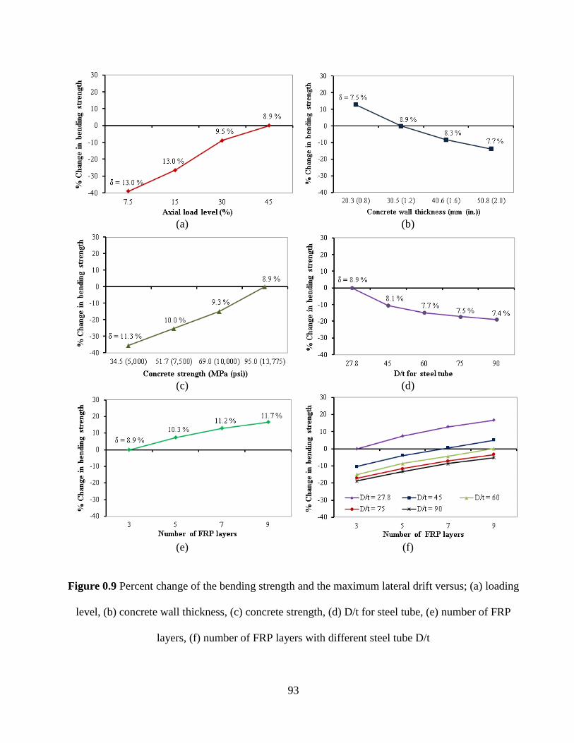
93

(a) (b)

(c) (d)

(e) (f)

Figure 0.9 Percent change of the bending strength and the maximum lateral drift versus; (a) loading

level, (b) concrete wall thickness, (c) concrete strength, (d) D/t for steel tube, (e) number of FRP

layers, (f) number of FRP layers with different steel tube D/t

94

Table 0.5 Summary of the parametric study results

Group Model

name Description

FE results Analytical results

Mcapacity Lateral

drift

Mcapacity

kip-ft kip-ft

A

DST-1

Load

Level

45.0% Po 24.9 8.9 27.1

DST-2A 30.0% Po 22.7 9.5 23.9

DST-3A 15.0% Po 18.4 13.0 19.2

DST-4A 7.5% Po 15.2 13.0 16.3

B

DST-1

Wall

thick

1.2 inch 24.9 8.9 27.1

DST-2B 0.8 inch 28.1 7.5 29.3

DST-3B 1.6 inch 22.9 8.3 24.8

DST-4B 2.0 inch 21.5 7.7 23.2

C

DST-1

𝑓𝑐′

13,775 psi 24.9 8.9 27.1

DST-2C 10,000 psi 21.2 9.3 23.3

DST-3C 7,500 psi 18.6 10.0 20.5

DST-4C 5,000 psi 16.0 11.3 18.3

D

DST-1

𝐷

𝑡

27.8 24.9 8.9 27.1

DST-2D 45.0 22.3 8.1 23.6

DST-3D 60.0 21.3 7.7 22.0

DST-4D 75.0 20.7 7.5 20.9

DST-5D 90.0 20.2 7.4 20.3

E

DST-1 Number

of FRP

layers

3 24.9 8.9 27.1

DST-2E 5 26.8 10.3 29.8

DST-3E 7 28.2 11.2 31.7

DST-4E 9 29.1 11.7 33.1

These specimens failed in two distinct failure modes. Column DST-1 failed as a result of

compression failure when an axial load of 45% Po was applied, while the other columns failed as a

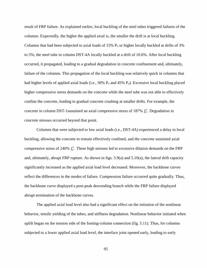
95

result of FRP failure. As explained earlier, local buckling of the steel tubes triggered failures of the

columns. Expectedly, the higher the applied axial is, the smaller the drift is at local buckling.

Columns that had been subjected to axial loads of 15% Po or higher locally buckled at drifts of 3%

to 5%; the steel tube in column DST-4A locally buckled at a drift of 10.6%. After local buckling

occurred, it propagated, leading to a gradual degradation in concrete confinement and, ultimately,

failure of the columns. This propagation of the local buckling was relatively quick in columns that

had higher levels of applied axial loads (i.e., 30% Po and 45% Po). Excessive local buckling placed

higher compressive stress demands on the concrete while the steel tube was not able to effectively

confine the concrete, leading to gradual concrete crushing at smaller drifts. For example, the

concrete in column DST-1sustained an axial compressive stress of 187% 𝑓𝑐′. Degradation in

concrete stresses occurred beyond that point.

Columns that were subjected to low axial loads (i.e., DST-4A) experienced a delay in local

buckling, allowing the concrete to remain effectively confined, and the concrete sustained axial

compressive stress of 240% 𝑓𝑐′. These high stresses led to excessive dilation demands on the FRP

and, ultimately, abrupt FRP rupture. As shown in figs. 5.9(a) and 5.10(a), the lateral drift capacity

significantly increased as the applied axial load level decreased. Moreover, the backbone curves

reflect the differences in the modes of failure. Compression failure occurred quite gradually. Thus,

the backbone curve displayed a post-peak descending branch while the FRP failure displayed

abrupt termination of the backbone curves.

The applied axial load level also had a significant effect on the initiation of the nonlinear

behavior, tensile yielding of the tubes, and stiffness degradation. Nonlinear behavior initiated when

uplift began on the tension side of the footing-column connection (fig. 5.11). Thus, for columns

subjected to a lower applied axial load level, the interface joint opened early, leading to early

96

stiffness degradation and early yielding of the steel tubes. The steel tubes in this group exhibited

tensile yielding at drifts between 1.4% and 2.6%. Expectedly, the higher the applied axial load is,

the higher the drift at the tensile yielding of the tube.

(a) (b)

Figure 0.10 Column-footing connection: (a) closed connection, and (b) uplift of the heel of the

connection

5.3.2 Effects of Concrete Wall Thickness on the Behavior of HC-FCS

Four columns, namely, DST-1, DST-2B, DST-3B, and DST-4B were studied with different

concrete wall thicknesses of 1.2 inch, 0.8 inch, 1.6 inch, and 2.0 inch, respectively. As shown in

figs. 5.9(b) and 5.10(b) as well as table 5.5, as the concrete wall thickness decreased, the column

strength increased. Decreasing the concrete wall thickness by 60% i.e., from 2.0 inches to 0.8

inches increased the bending strength 30% i.e., from 21.5 kip-ft in column DST-4B to 29.8 kip-ft in

column DST-2B.

The increase in the strength of columns having smaller wall thickness occurred since the

lever arm between the tensile forces in the steel tube and the compression forces in concrete and the

steel tube increased in relation to decreasing the concrete wall thickness. Moreover, since all

columns have the same FRP and steel rigidities, confinement of columns having smaller concrete

wall thickness was relatively higher. The concrete in the case of column DST-2B sustained

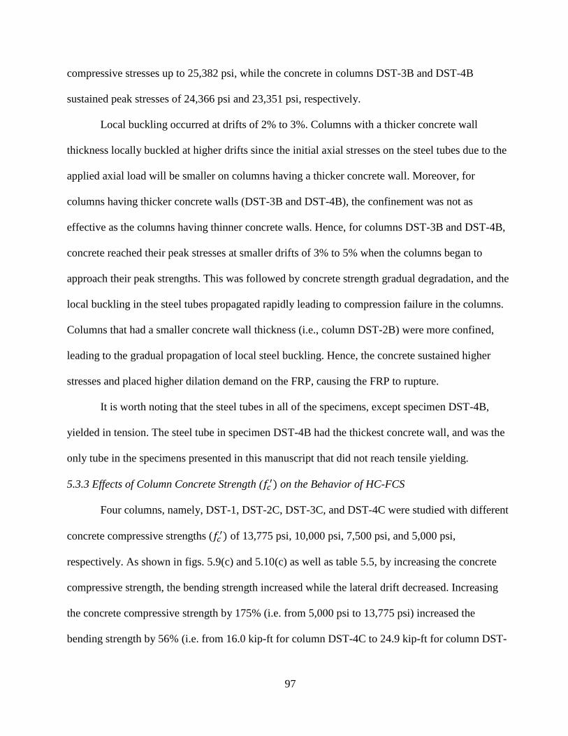
97

compressive stresses up to 25,382 psi, while the concrete in columns DST-3B and DST-4B

sustained peak stresses of 24,366 psi and 23,351 psi, respectively.

Local buckling occurred at drifts of 2% to 3%. Columns with a thicker concrete wall

thickness locally buckled at higher drifts since the initial axial stresses on the steel tubes due to the

applied axial load will be smaller on columns having a thicker concrete wall. Moreover, for

columns having thicker concrete walls (DST-3B and DST-4B), the confinement was not as

effective as the columns having thinner concrete walls. Hence, for columns DST-3B and DST-4B,

concrete reached their peak stresses at smaller drifts of 3% to 5% when the columns began to

approach their peak strengths. This was followed by concrete strength gradual degradation, and the

local buckling in the steel tubes propagated rapidly leading to compression failure in the columns.

Columns that had a smaller concrete wall thickness (i.e., column DST-2B) were more confined,

leading to the gradual propagation of local steel buckling. Hence, the concrete sustained higher

stresses and placed higher dilation demand on the FRP, causing the FRP to rupture.

It is worth noting that the steel tubes in all of the specimens, except specimen DST-4B,

yielded in tension. The steel tube in specimen DST-4B had the thickest concrete wall, and was the

only tube in the specimens presented in this manuscript that did not reach tensile yielding.

5.3.3 Effects of Column Concrete Strength (𝑓𝑐′) on the Behavior of HC-FCS

Four columns, namely, DST-1, DST-2C, DST-3C, and DST-4C were studied with different

concrete compressive strengths (𝑓𝑐′) of 13,775 psi, 10,000 psi, 7,500 psi, and 5,000 psi,

respectively. As shown in figs. 5.9(c) and 5.10(c) as well as table 5.5, by increasing the concrete

compressive strength, the bending strength increased while the lateral drift decreased. Increasing

the concrete compressive strength by 175% (i.e. from 5,000 psi to 13,775 psi) increased the

bending strength by 56% (i.e. from 16.0 kip-ft for column DST-4C to 24.9 kip-ft for column DST-

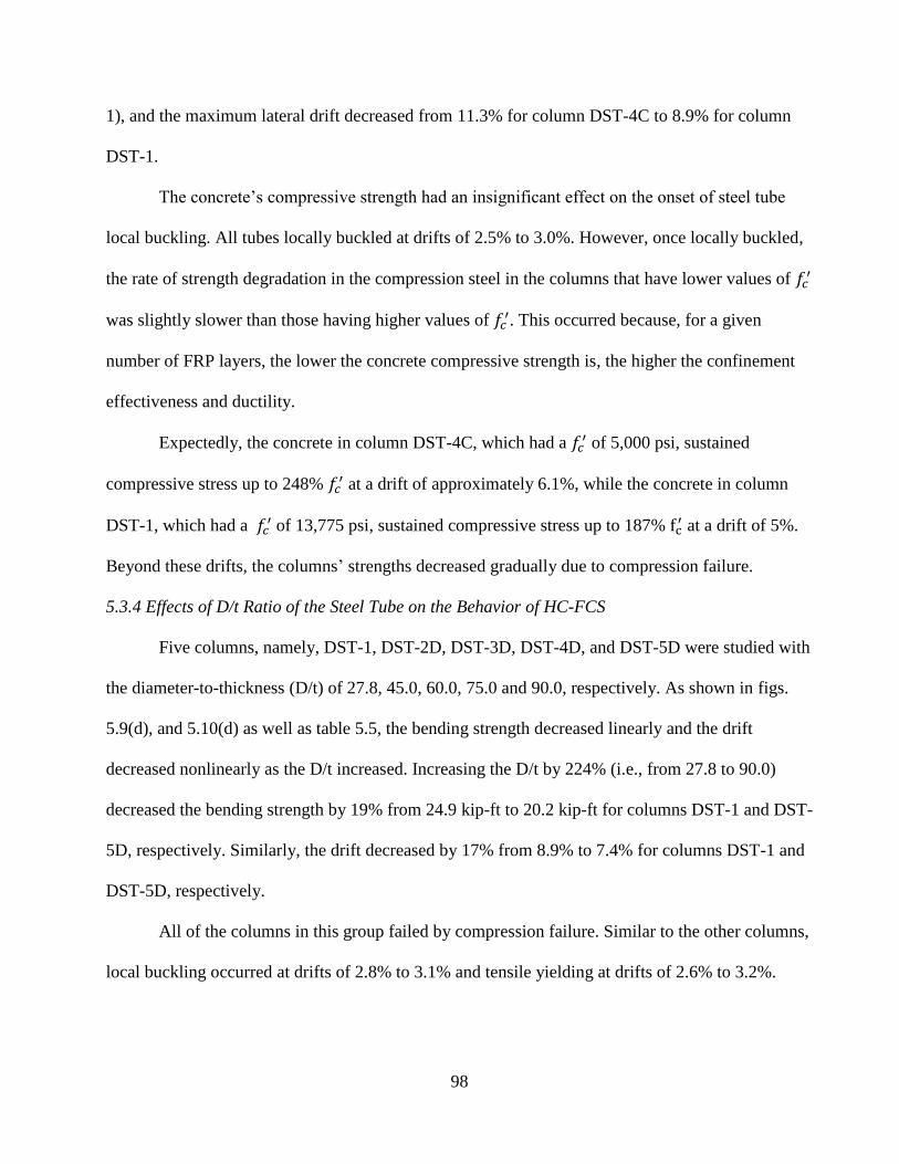
98

1), and the maximum lateral drift decreased from 11.3% for column DST-4C to 8.9% for column

DST-1.

The concrete’s compressive strength had an insignificant effect on the onset of steel tube

local buckling. All tubes locally buckled at drifts of 2.5% to 3.0%. However, once locally buckled,

the rate of strength degradation in the compression steel in the columns that have lower values of 𝑓𝑐′

was slightly slower than those having higher values of 𝑓𝑐′. This occurred because, for a given

number of FRP layers, the lower the concrete compressive strength is, the higher the confinement

effectiveness and ductility.

Expectedly, the concrete in column DST-4C, which had a 𝑓𝑐′ of 5,000 psi, sustained

compressive stress up to 248% 𝑓𝑐′ at a drift of approximately 6.1%, while the concrete in column

DST-1, which had a 𝑓𝑐′ of 13,775 psi, sustained compressive stress up to 187% fc

′ at a drift of 5%.

Beyond these drifts, the columns’ strengths decreased gradually due to compression failure.

5.3.4 Effects of D/t Ratio of the Steel Tube on the Behavior of HC-FCS

Five columns, namely, DST-1, DST-2D, DST-3D, DST-4D, and DST-5D were studied with

the diameter-to-thickness (D/t) of 27.8, 45.0, 60.0, 75.0 and 90.0, respectively. As shown in figs.

5.9(d), and 5.10(d) as well as table 5.5, the bending strength decreased linearly and the drift

decreased nonlinearly as the D/t increased. Increasing the D/t by 224% (i.e., from 27.8 to 90.0)

decreased the bending strength by 19% from 24.9 kip-ft to 20.2 kip-ft for columns DST-1 and DST-

5D, respectively. Similarly, the drift decreased by 17% from 8.9% to 7.4% for columns DST-1 and

DST-5D, respectively.

All of the columns in this group failed by compression failure. Similar to the other columns,

local buckling occurred at drifts of 2.8% to 3.1% and tensile yielding at drifts of 2.6% to 3.2%.

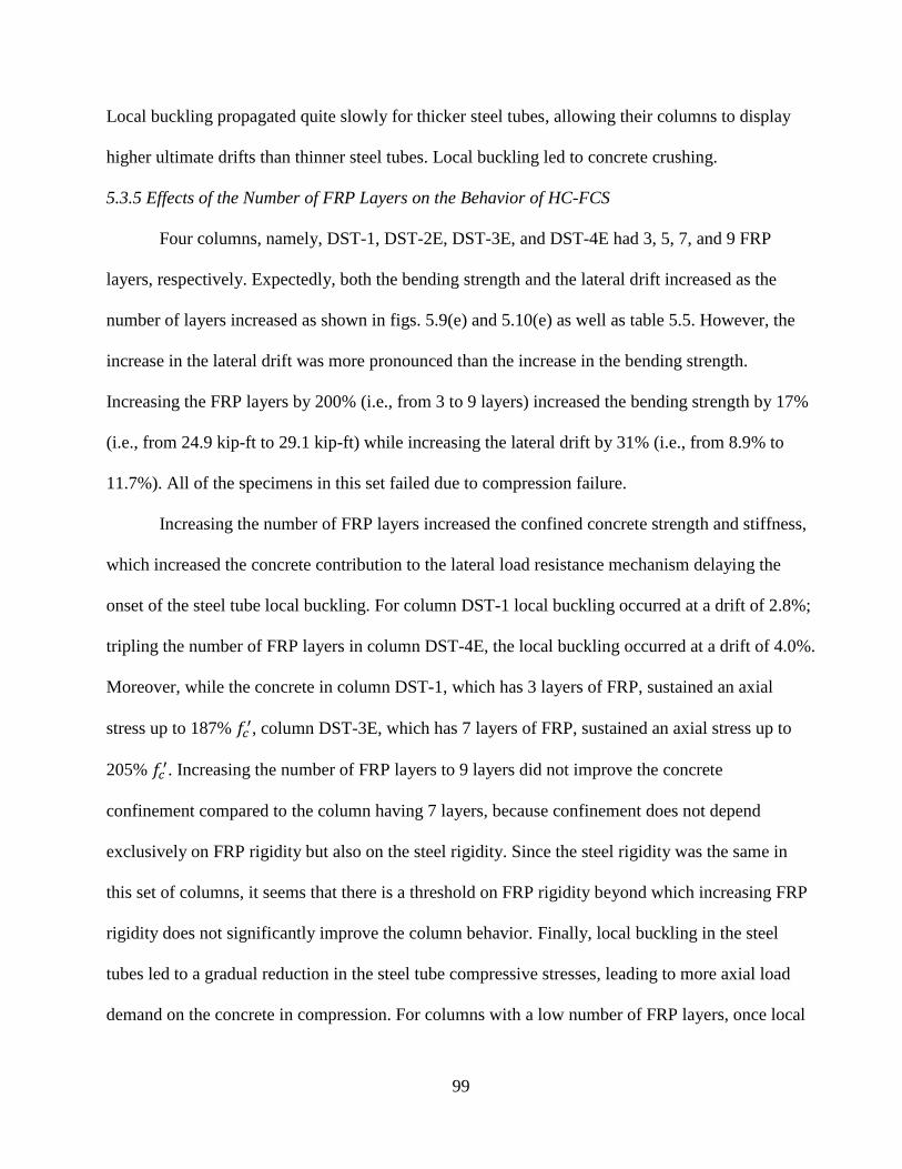
99

Local buckling propagated quite slowly for thicker steel tubes, allowing their columns to display

higher ultimate drifts than thinner steel tubes. Local buckling led to concrete crushing.

5.3.5 Effects of the Number of FRP Layers on the Behavior of HC-FCS

Four columns, namely, DST-1, DST-2E, DST-3E, and DST-4E had 3, 5, 7, and 9 FRP

layers, respectively. Expectedly, both the bending strength and the lateral drift increased as the

number of layers increased as shown in figs. 5.9(e) and 5.10(e) as well as table 5.5. However, the

increase in the lateral drift was more pronounced than the increase in the bending strength.

Increasing the FRP layers by 200% (i.e., from 3 to 9 layers) increased the bending strength by 17%

(i.e., from 24.9 kip-ft to 29.1 kip-ft) while increasing the lateral drift by 31% (i.e., from 8.9% to

11.7%). All of the specimens in this set failed due to compression failure.

Increasing the number of FRP layers increased the confined concrete strength and stiffness,

which increased the concrete contribution to the lateral load resistance mechanism delaying the

onset of the steel tube local buckling. For column DST-1 local buckling occurred at a drift of 2.8%;

tripling the number of FRP layers in column DST-4E, the local buckling occurred at a drift of 4.0%.

Moreover, while the concrete in column DST-1, which has 3 layers of FRP, sustained an axial

stress up to 187% 𝑓𝑐′, column DST-3E, which has 7 layers of FRP, sustained an axial stress up to

205% 𝑓𝑐′. Increasing the number of FRP layers to 9 layers did not improve the concrete

confinement compared to the column having 7 layers, because confinement does not depend

exclusively on FRP rigidity but also on the steel rigidity. Since the steel rigidity was the same in

this set of columns, it seems that there is a threshold on FRP rigidity beyond which increasing FRP

rigidity does not significantly improve the column behavior. Finally, local buckling in the steel

tubes led to a gradual reduction in the steel tube compressive stresses, leading to more axial load

demand on the concrete in compression. For columns with a low number of FRP layers, once local

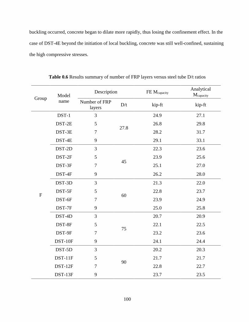
100

buckling occurred, concrete began to dilate more rapidly, thus losing the confinement effect. In the

case of DST-4E beyond the initiation of local buckling, concrete was still well-confined, sustaining

the high compressive stresses.

Table 0.6 Results summary of number of FRP layers versus steel tube D/t ratios

Group Model

name

Description FE Mcapacity Analytical

Mcapacity

Number of FRP

layers D/t kip-ft kip-ft

F

DST-1 3

27.8

24.9 27.1

DST-2E 5 26.8 29.8

DST-3E 7 28.2 31.7

DST-4E 9 29.1 33.1

DST-2D 3

45

22.3 23.6

DST-2F 5 23.9 25.6

DST-3F 7 25.1 27.0

DST-4F 9 26.2 28.0

DST-3D 3

60

21.3 22.0

DST-5F 5 22.8 23.7

DST-6F 7 23.9 24.9

DST-7F 9 25.0 25.8

DST-4D 3

75

20.7 20.9

DST-8F 5 22.1 22.5

DST-9F 7 23.2 23.6

DST-10F 9 24.1 24.4

DST-5D 3

90

20.2 20.3

DST-11F 5 21.7 21.7

DST-12F 7 22.8 22.7

DST-13F 9 23.7 23.5

101

5.3.6 Effects of the Number of FRP Layers Combined with D/t Ratio

The number of FRP layers versus D/t ratios of the steel tubes was investigated last. Twenty

columns were investigated numerically as stated in table 5.6. Four different numbers of FRP layers

of 3, 5, 7, and 9 were studied in a matrix with five steel tube D/t ratios of 27.8, 45.0, 60.0, 75.0, and

90.0. The bending strength increased as the number of layers increased regardless of the steel tube

D/t ratio as presented in fig. 5.10(f). However, the bending strength decreased as the steel tube D/t

ratio increased for the same number of FRP layers. The relationship between the number of FRP

layers and the bending strength was nearly linear, regardless of the steel tube D/t ratio. It is worth

noting that, for a given number of FRP layers, the rate of increase in the bending decreases with the

increasing D/t ratio.

102

Chapter 6 Analysis of Vehicle Collision with Reinforced Concrete Bridge Columns

6.1 Research Significance

While several studies investigated the issue of vehicle impact with concrete columns, few

studies investigated the effect of the different construction detailing and vehicle parameters on the

performance of the column. This report used detailed finite element analyses to investigate the

effects of 13 different parameters including the concrete material model, unconfined compressive

strength (𝑓𝑐′), material strain rate, percentage of longitudinal reinforcement, hoop reinforcement,

column span-to-depth ratio, column diameter, the top boundary conditions, axial load level, vehicle

velocity, vehicle mass, clear zone distance, and soil depth above the top of the column footing on

the dynamic and static impact forces. Comparisons between the ESF of the AASHTO-LRFD 600

kips and the ESF calculated using different approaches are presented as well. Furthermore, the

constant impact load used in AASHTO-LRFD does not consider the vehicle mass nor the velocity.

Hence, it may be anticipated that the given impact load will be conservative in some occasions and

unconservative in other occasions. This report presents a new equation to directly calculate the ESF

given the vehicle’s mass and velocity without the need to run crash analysis. Similarly, a simplified

equation for the Eurocode equation is presented to directly calculate the ESF without a crash

analysis.

6.2 Verifying the Finite Element Modeling of a Vehicle Colliding with a Bridge Pier

Experiments conducted on vehicle collisions with concrete columns are both difficult and

expensive. Finite element analysis (FEA) is considered an attractive approach because it is

economical, reliable, and easy to implement. The FEA of a collision event requires a combination

of vehicle and concrete structure modeling.

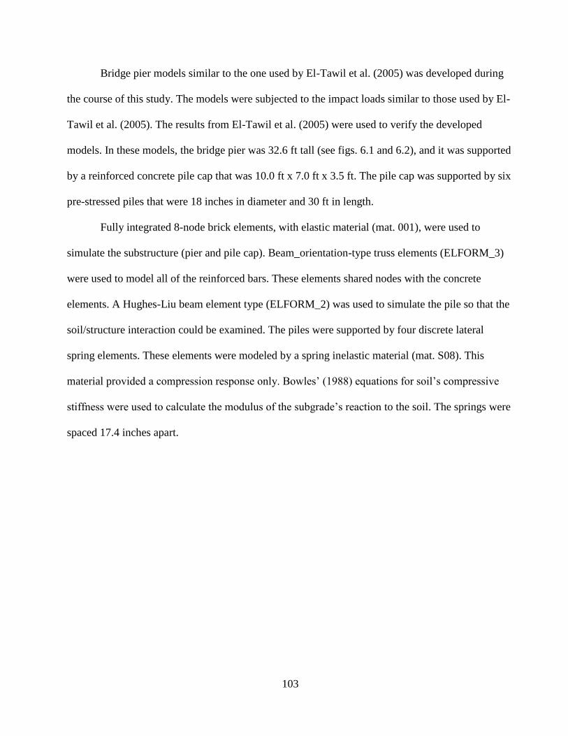
103

Bridge pier models similar to the one used by El-Tawil et al. (2005) was developed during

the course of this study. The models were subjected to the impact loads similar to those used by El-

Tawil et al. (2005). The results from El-Tawil et al. (2005) were used to verify the developed

models. In these models, the bridge pier was 32.6 ft tall (see figs. 6.1 and 6.2), and it was supported

by a reinforced concrete pile cap that was 10.0 ft x 7.0 ft x 3.5 ft. The pile cap was supported by six

pre-stressed piles that were 18 inches in diameter and 30 ft in length.

Fully integrated 8-node brick elements, with elastic material (mat. 001), were used to

simulate the substructure (pier and pile cap). Beam_orientation-type truss elements (ELFORM_3)

were used to model all of the reinforced bars. These elements shared nodes with the concrete

elements. A Hughes-Liu beam element type (ELFORM_2) was used to simulate the pile so that the

soil/structure interaction could be examined. The piles were supported by four discrete lateral

spring elements. These elements were modeled by a spring inelastic material (mat. S08). This

material provided a compression response only. Bowles’ (1988) equations for soil’s compressive

stiffness were used to calculate the modulus of the subgrade’s reaction to the soil. The springs were

spaced 17.4 inches apart.

104

Figure 0.1 3D- view of the FE model for verification against El-Tawil’s et al. (2005) results

Note: soil subgrade springs are not shown for simplicity

The bridge superstructure was composed of a composite steel-concrete box girder. Thirty-

six Belytschko-Schwer resultant beam-type (ELFORM_2) elements were used to simulate two

adjacent steel girders. This superstructure’s transformed steel cross-sectional area was 124 in2. The

strong moment of inertia (the Iyy about the vertical axis) was 2.0 x 105 in4, and the weak moment of

inertia (the Izz about the horizontal axis) was 6.7 x 104 in4. The superstructure’s two unequal spans

were 175 ft and 165 ft, respectively. This superstructure was assumed to be pinned at the far ends.

The Hughes-Liu beam-type element (ELFORM_2) was used to simulate the bridge bearings located

under the superstructure. These bearings were 1.5 inches thick and 8 inches x 8 inches in the cross-

section. The bridge bearing’s shear modulus was 88.0 psi.

A Chevrolet pickup’s reduced finite element model was used to study the vehicle’s collision

with a bridge pier (fig. 6.3a). A surface-to-surface contact element was used between the vehicle

and the bridge pier in the finite element models; the coefficient of friction was 0.3. The vehicle

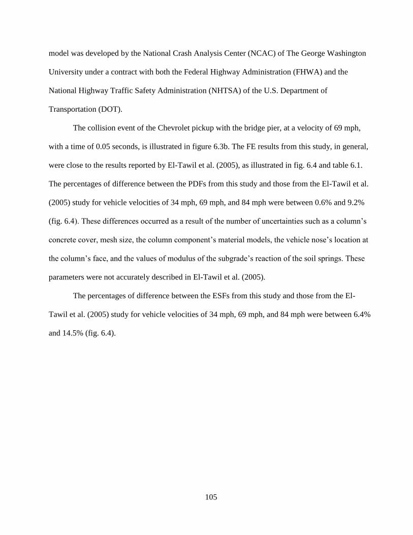
105

model was developed by the National Crash Analysis Center (NCAC) of The George Washington

University under a contract with both the Federal Highway Administration (FHWA) and the

National Highway Traffic Safety Administration (NHTSA) of the U.S. Department of

Transportation (DOT).

The collision event of the Chevrolet pickup with the bridge pier, at a velocity of 69 mph,

with a time of 0.05 seconds, is illustrated in figure 6.3b. The FE results from this study, in general,

were close to the results reported by El-Tawil et al. (2005), as illustrated in fig. 6.4 and table 6.1.

The percentages of difference between the PDFs from this study and those from the El-Tawil et al.

(2005) study for vehicle velocities of 34 mph, 69 mph, and 84 mph were between 0.6% and 9.2%

(fig. 6.4). These differences occurred as a result of the number of uncertainties such as a column’s

concrete cover, mesh size, the column component’s material models, the vehicle nose’s location at

the column’s face, and the values of modulus of the subgrade’s reaction of the soil springs. These

parameters were not accurately described in El-Tawil et al. (2005).

The percentages of difference between the ESFs from this study and those from the El-

Tawil et al. (2005) study for vehicle velocities of 34 mph, 69 mph, and 84 mph were between 6.4%

and 14.5% (fig. 6.4).

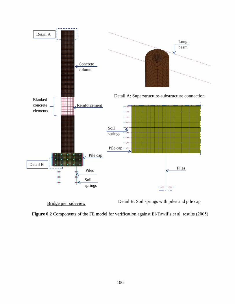
106

Bridge pier sideview

Detail A: Superstructure-substructure connection

Detail B: Soil springs with piles and pile cap

Figure 0.2 Components of the FE model for verification against El-Tawil’s et al. results (2005)

Detail B

Detail A

Blanked

concrete

elements

Reinforcement

Pile cap

Concrete

column

Piles Piles

Soil

springs

Pile cap

Soil

springs

Long.

beam

107

(a) (b)

Figure 0.3 The reduced FE model of Chevrolet pickup: (a) 3D-view, and (b) side view of the

collision event of the reduced FE model of Chevrolet pickup with bridge pier (velocity = 69 mph

and time = 0.05 second)

(a) (b)

(c) (d)

Figure 0.4 FE results from current study versus those from El-Tawil et al. (2005) FE results; (a)

vehicle velocity of 34 mph, (b) vehicle velocity of 69 mph, (c) vehicle velocity of 84 mph, and (d)

PDF and ESF versus the vehicle velocities

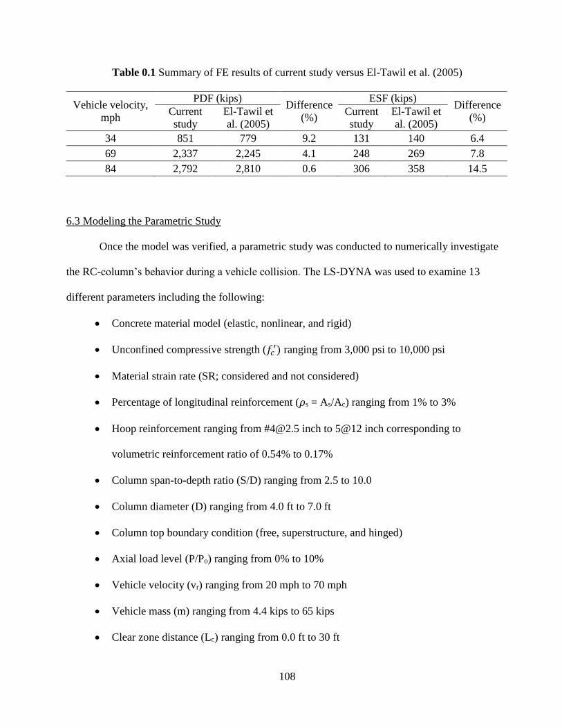
108

Table 0.1 Summary of FE results of current study versus El-Tawil et al. (2005)

Vehicle velocity,

mph

PDF (kips) Difference

(%)

ESF (kips) Difference

(%) Current

study

El-Tawil et

al. (2005)

Current

study

El-Tawil et

al. (2005)

34 851 779 9.2 131 140 6.4

69 2,337 2,245 4.1 248 269 7.8

84 2,792 2,810 0.6 306 358 14.5

6.3 Modeling the Parametric Study

Once the model was verified, a parametric study was conducted to numerically investigate

the RC-column’s behavior during a vehicle collision. The LS-DYNA was used to examine 13

different parameters including the following:

Concrete material model (elastic, nonlinear, and rigid)

Unconfined compressive strength (𝑓𝑐′) ranging from 3,000 psi to 10,000 psi

Material strain rate (SR; considered and not considered)

Percentage of longitudinal reinforcement (𝜌s = As/Ac) ranging from 1% to 3%

Hoop reinforcement ranging from #[email protected] inch to 5@12 inch corresponding to

volumetric reinforcement ratio of 0.54% to 0.17%

Column span-to-depth ratio (S/D) ranging from 2.5 to 10.0

Column diameter (D) ranging from 4.0 ft to 7.0 ft

Column top boundary condition (free, superstructure, and hinged)

Axial load level (P/Po) ranging from 0% to 10%

Vehicle velocity (vr) ranging from 20 mph to 70 mph

Vehicle mass (m) ranging from 4.4 kips to 65 kips

Clear zone distance (Lc) ranging from 0.0 ft to 30 ft

mailto:#[email protected]

109

Soil depth above the top of the column footing (ds) ranging from 1.7 ft to 5.0 ft

Thirty-three columns (from C0 to C32) were investigated. Column C0 was used as a

reference column. The ranges of selected variables for the columns with regard to the examined

parameters are summarized in table 6.2. It should be noted that some of the selected parameters

may not be common in practice. However, they were used to fully understand the performance of

the columns under a wide spectrum of parameters.

6.3.1 Geometry

The columns investigated in this study were supported on a concrete footing that had fixed

boundary condition at its bottom. All of the columns, except for C17 and C18, were hinged at the

top ends. Column C17 was free at the top end, while column C18 had superstructure attached at its

top as explained in the verification section. Each column had a circular cross-section with a

diameter (D) that was between 4.0 ft and 7.0 ft, with 5.0 ft being the common diameter (fig. 6.5).

The column’s height (H) ranged from 12.5 ft to 50.0 ft, with 25.0 ft being the common height. The

column span-to-depth ratios (S/D) ranged from 2.5 to 10, with 5.0 being the common span-to-depth

ratio. The soil depth above the top of the footing (ds) ranged from 1.7 ft to 4.9 ft, with 3.3 ft being

the common soil depth.

The percentage of longitudinal steel reinforcement (𝜌s) ranged from 1.0% to 3.0%, with

1.0% being the common percent. The hoop reinforcement size ranged from #4 to #6, with #5 being

the common hoop reinforcement size. The hoop reinforcement spacing ranged from 2.5 inches to

12 inches, with 4 inches being the common hoop reinforcement spacing.

The column’s axial load (P) ranged from 0% to 10% of Po, with 5% of Po being the common

axial load where Po was calculated by eqn. (2.1).

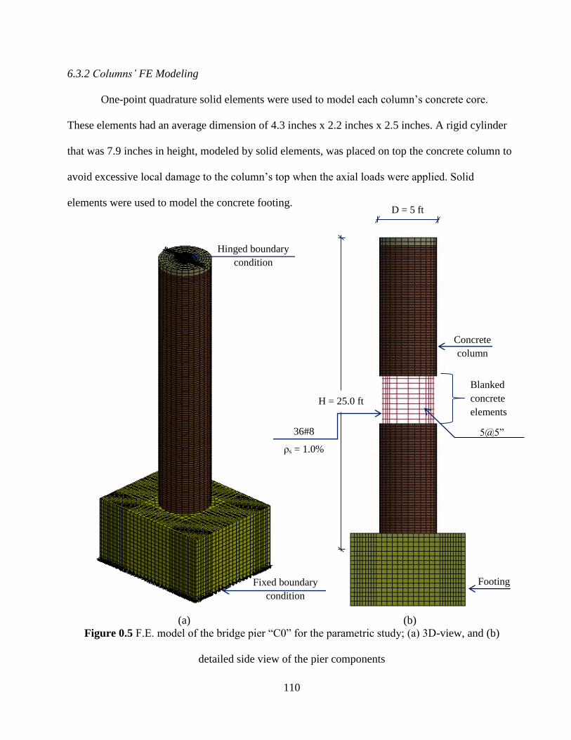
110

6.3.2 Columns’ FE Modeling

One-point quadrature solid elements were used to model each column’s concrete core.

These elements had an average dimension of 4.3 inches x 2.2 inches x 2.5 inches. A rigid cylinder

that was 7.9 inches in height, modeled by solid elements, was placed on top the concrete column to

avoid excessive local damage to the column’s top when the axial loads were applied. Solid

elements were used to model the concrete footing.

(a) (b)

Figure 0.5 F.E. model of the bridge pier “C0” for the parametric study; (a) 3D-view, and (b)

detailed side view of the pier components

Blanked

concrete

elements

Footing

Concrete

column

36#8

ρs = 1.0%

H = 25.0 ft

D = 5 ft

5@5”

Hinged boundary

condition

Fixed boundary

condition

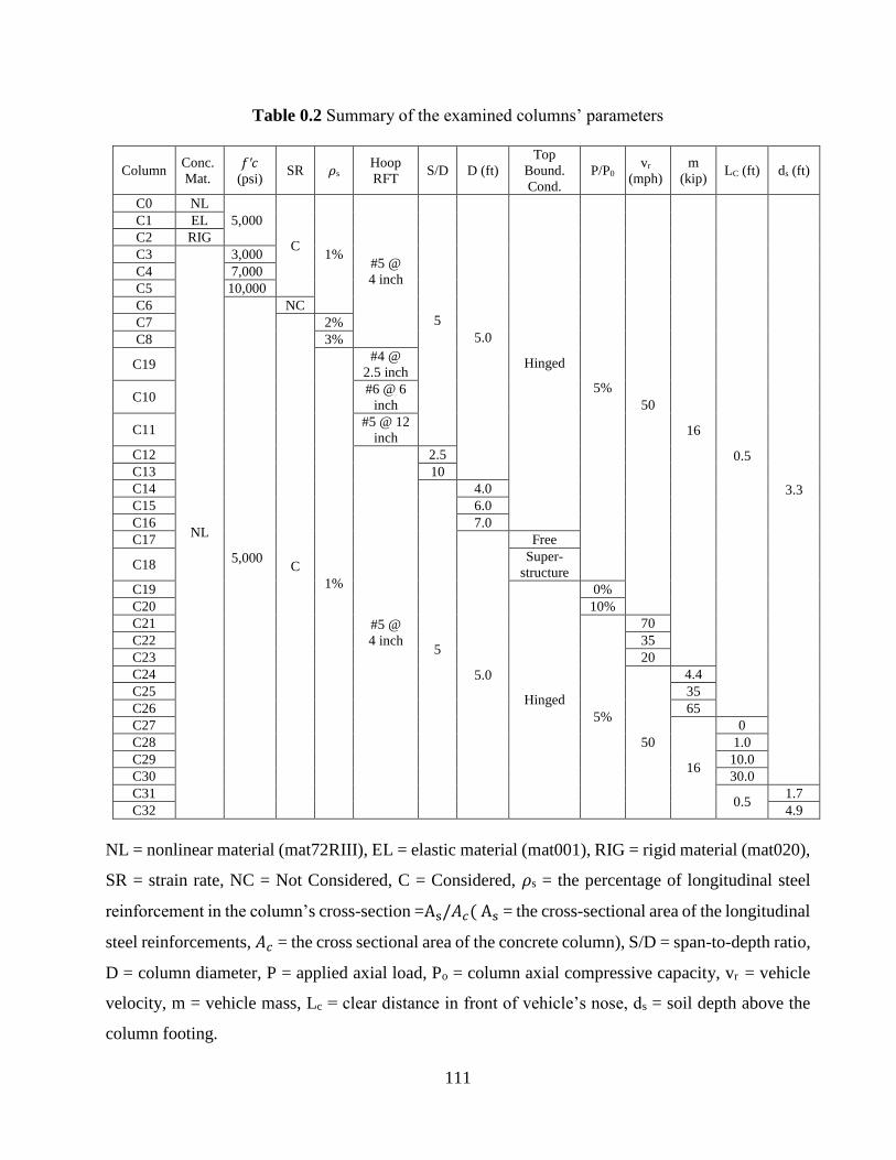
111

Table 0.2 Summary of the examined columns’ parameters

Column Conc.

Mat.

𝑓′𝑐

(psi) SR 𝜌s

Hoop

RFT S/D D (ft)

Top

Bound.

Cond.

P/P0 vr

(mph)

m

(kip) LC (ft) ds (ft)

C0 NL

5,000

C 1%

#5 @

4 inch

5

5.0

Hinged

5%

50

16

0.5

3.3

C1 EL

C2 RIG

C3

NL

3,000

C4 7,000

C5 10,000

C6

5,000

NC

C7

C

2%

C8 3%

C19

1%

#4 @

2.5 inch

C10 #6 @ 6

inch

C11 #5 @ 12

inch

C12

#5 @

4 inch

2.5

C13 10

C14

5

4.0

C15 6.0

C16 7.0

C17

5.0

Free

C18 Super-

structure

C19

Hinged

0%

C20 10%

C21

5%

70

C22 35

C23 20

C24

50

4.4

C25 35

C26 65

C27

16

0

C28 1.0

C29 10.0

C30 30.0

C31 0.5

1.7

C32 4.9

NL = nonlinear material (mat72RIII), EL = elastic material (mat001), RIG = rigid material (mat020),

SR = strain rate, NC = Not Considered, C = Considered, 𝜌s = the percentage of longitudinal steel

reinforcement in the column’s cross-section =As/𝐴𝑐( As = the cross-sectional area of the longitudinal

steel reinforcements, 𝐴𝑐 = the cross sectional area of the concrete column), S/D = span-to-depth ratio,

D = column diameter, P = applied axial load, Po = column axial compressive capacity, vr = vehicle

velocity, m = vehicle mass, Lc = clear distance in front of vehicle’s nose, ds = soil depth above the

column footing.

112

An hourglass control was used to avoid spurious singular modes (e.g., hourglass modes).

The hourglass value for each of the models was taken as the default value 0.10, with an hourglass

control type_4 (Flanagan-Belytschko stiffness form). Both the longitudinal and the hoop

reinforcements were modeled by beam_orientation elements. All of the beam elements within the

reinforcement were constrained with the concrete column and the footing by “Lagrange in solid.”

The column’s concrete cover was defined to spall at an axial compressive strain exceeding 0.005

(Caltrans 2006).

6.3.3 Material Models

Two different concrete material models have been used in the literature to assess the impact

forces on bridge columns, namely, the elastic isotropic material mat001 and rigid material model

mat020. Using an elastic material allows the evaluation of the impact force assuming that the

column will remain elastic (El-Tawil et al. 2005). Using rigid material model does not allow any

deformations to take place in the columns (Buth et al. 2010). Since both material models respond

elastically, the energy dissipation by the inelastic deformation in the column is ignored. Thus, the

impact forces calculated with these two material models represent the impact forces’ upper bounds.

The AASHTO-LRFD, however, considers vehicle impact to be an extreme load. Therefore, a

column’s nonlinear behavior is both expected and allowed. Hence, this research investigated the

effect of three different concrete material models including elastic (mat001), rigid (mat020), and

nonlinear (mat72RIII) on the response of bridge column to vehicle impact.

For elastic material, the elastic modulus and Poisson’s ratio are the only parameters required

to define this material model. These parameters were also used for the rigid material in determining

the sliding interface parameters of the contact elements between the vehicle and the column. The

elastic modulus (E) was calculated according to ACI-318 (2011), and considering the dynamic

113

increase factor (DIF), factor (E = 4,750 √DIF ∗ 𝑓𝑐′ ) and the Poisson’s ratio was taken as 0.20

(Mehta and Monteiro 2006). The DIF factor is explained later in this section.

A nonlinear concrete material model (mat72RIII) was used for all columns and footings that

were examined in this study except for C1, C2, and their footings. The model had three shear

failure surfaces: yield, maximum, and residual (Malvar et al. 1997). Given 𝑓𝑐′ and ω, the yield

failure surfaces of this model were generated automatically. The fractional dilation parameter (ω)

that takes into consideration any volumetric change occurring in the concrete was taken as the

default value of 0.50.

Loading strain rates may play an essential role in a structure’s response. The DIF is

typically used to describe the increase in concrete’s strength under dynamic loading as compared to

static loading (Malvar and Ross 1998; Bischoff and Perry 1991; Williams 1994; Fu et al. 1991).

Malvar and Ross (1998) modified the CEB model code for use with strain rate effects and

implemented the modified model into a LS-DYNA format (CEB-FIP 1990). For example, when

concrete has a compressive strength (𝑓𝑐′) of 5,000 psi, and is subjected to a compressive load with a

strain rate of 100 s-1 (common for impact loading), the DIF will be 2.21 in compression and 7.52 in

tension (Sierakowsi and Chaturved 1997). The effect of a high strain rate is quite significant with

regard to concrete’s tensile strength compared to concrete’s compressive strength. This occurred

since tension cracks do not have enough time to propagate through concrete because the loading

time is too short.

6.3.4 Steel Reinforcement

An elasto-plastic constitutive model, mat003-plastic_kinamatic, was used for steel

reinforcement. The following five parameters were needed to define this material model: the elastic

modulus (E), the yield stress, Poisson’s ratio, the tangent modulus, and the ultimate plastic strain.

114

These parameters were assigned the following values: 29,000 ksi, 60,900 psi, 0.30, 160 ksi, and

0.12, respectively (Caltrans 2006). To consider strain rate effect, Cowper-Symonds’s (1957) model

was adopted. Parameters p and c were assigned as a means for identifying the strain rate effect. The

constants p and c were taken as 5 and 40, respectively (Yan and Yali 2012). Substituting these two

constants into Cowper-Symonds’s equation at a strain rate of 100 s-1 produces a dynamic yield

stress that is 2.20 times the static yield stress. The elastic modulus of steel does not considerably

change under impact loading (Campbell 1954).

6.3.5 Vehicles FE Models

Two vehicle models were used in this study: a Ford reduced model (35,353 elements) single

unit truck (SUT) and a detailed model (58,313 elements) Chevrolet C2500 pickup (fig. 6.6). These

models were downloaded from the NCAC website. Experimental tests involving head-on collisions

were conducted to verify each model (Zaouk et al. 1996; Mohan et al. 2003).

Different vehicle impact speeds were investigated during this research ranging from 20 mph

to 70 mph, with 50 mph being the common velocity. The mass of the vehicle ranged from 4.4 kips

to 65 kips, with 18 kips being the common mass. The Chevrolet C2500 pickup was used as the

vehicle for the mass of 4.4 kips, and the Ford SUT was used for the other models. The Ford SUT’s

mass increased by increasing the value of the added mass. Automatic_surface_to_surface contact

elements by parts with the contact factor SOFT=1 were used between the vehicle and the RC-

column (Bala 2001).

If the bridge pier was located inside the clear zone (the total roadside border area, starting at

the edge of the traveled way, available for safe use by an errant vehicle) without a crashworthy

barrier, the design of the pier must include the collision force (KDoT 2013). The effect of the clear

zone distance (Lc) was examined here by changing the distance between the vehicle’s nose and the

115

column’s face. The clear zone distance ranged from 0.0 ft to 30.0 ft, with 0.5 ft being the common

clear zone distance.

(a) (b)

Figure 0.6 3D-view of the FE model: (a) the Ford single unit truck, (b) Chevrolet pickup detailed

model

6.4 Results and Discussion of the Parametric Study

6.4.1 Performance Levels

While few researchers have attempted to assign limit states to bridge columns under vehicle

impact (Agrawal et al. 2013; Sharma et al. 2012), there has been no consensus among researchers

on the damage state at the different limit states. During the course of this report, the authors defined

three different limit states. Performance level P1 was assigned when no bar buckling took place

during the analysis. The performance level P2, heavy damage, was assigned when less than 20% of

the longitudinal rebar buckled. The performance level P3 was assigned when at least 20% of

116

longitudinal rebar buckled, which is considered to be the column’s failure. Figure 6.7a and table 6.3

present the performance levels of all of the columns. Approximately 73%, 15%, and 12% of the

columns were assigned to performance levels P1, P2, and P3, respectively. The columns C14, C21,

C25, and C26 failed under the vehicle impact load. These impact cases are characterized by small

column diameter of 4 ft, high speed vehicle of 70 mph, and heavy mass greater than 35 kips. The

columns C3, C6, C12, C17, and C30 suffered heavy damage. These impact cases are characterized

by low concrete strength of 3,000 psi, excluding strain rate effect, low column’s aspect ratio of 2.5,

free top boundary condition, and long clear zone distance of 30 ft.

6.4.2 General Comparisons

Figure 6.7b and table 6.3 present the ESF and the columns’ shear capacity normalized by

the ESF of the AASHTO-LRFD (600 kips) for all of the columns. In addition, table 6.3 summarizes

the PDFs normalized by the ESF of the AASHTO-LRFD for all of the columns. As shown in the

figure and table, the differences between the ESF approaches were highly varied from case to case.

The differences between the maximum and the minimum values of ESF calculated using the

different approaches for a given column ranged from 7% (C2) to 140% (C14). Furthermore, the

SBESF represents the upper bound for 73% of the cases while ECESF represents the lower bound for

85% of the columns. The SBESF of 27% of the examined columns exceeded or equaled the ESF of

the AASHTO-LRFD (600 kips). The ESF calculated using the PTMSA exceeded the ESF of the

AASHTO-LRFD for 9% of the examined columns. In general, the ESF of the Eurocode (ECESF)

was typically lower than the ESF of the AASHTO-LRFD except for the columns C25 and C26 of

the heavy vehicles of masses more than 35 kips.

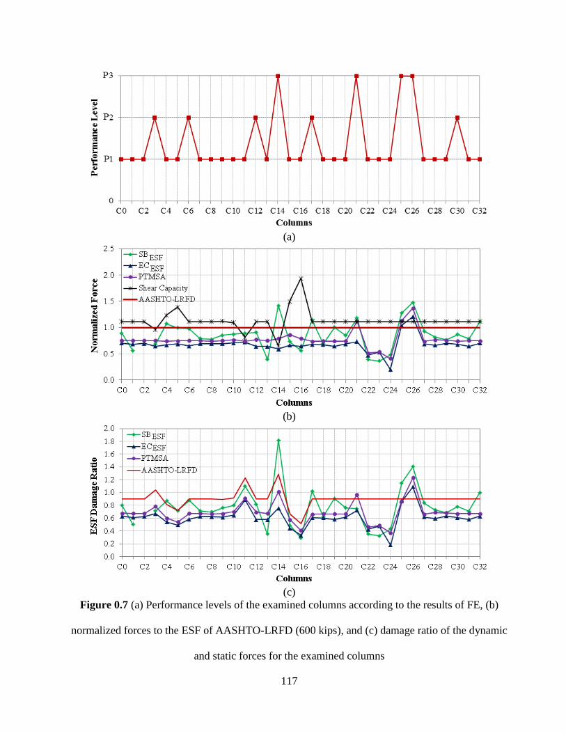
117

(a)

(b)

(c)

Figure 0.7 (a) Performance levels of the examined columns according to the results of FE, (b)

normalized forces to the ESF of AASHTO-LRFD (600 kips), and (c) damage ratio of the dynamic

and static forces for the examined columns

118

The results of FE will be used as a basis for comparing the best approach in calculating the

ESF. Columns that reach performance level P3 will be called “failed columns” while all other

columns will be called “unfailed columns.” Among the investigated approaches, if the ESF

according to a given approach is higher than the shear capacity of this column, the column will be

considered a failed column. Otherwise, it is an unfailed column. Equations 6.1 and 6.2 summarize

these characteristics as follows:

Safety according to FE =

𝑡𝑟𝑢𝑒 𝑣𝑎𝑙𝑢𝑒 𝑜𝑓 {𝑃1 𝑜𝑟 𝑃2 (𝑢𝑛𝑓𝑎𝑖𝑙𝑒𝑑 𝑐𝑜𝑙𝑢𝑚𝑛)𝑃3 (𝑓𝑎𝑖𝑙𝑒𝑑 𝑐𝑜𝑙𝑢𝑚𝑛)

(6.1)

Safety according to the different approaches =

𝑡𝑟𝑢𝑒 𝑣𝑎𝑙𝑢𝑒 𝑜𝑓 {𝐸𝑆𝐹 ≤ 𝑠ℎ𝑒𝑎𝑟 𝑐𝑎𝑝𝑎𝑐𝑖𝑡𝑦 (𝑢𝑛𝑓𝑎𝑖𝑙𝑒𝑑 𝑐𝑜𝑙𝑢𝑚𝑛)𝐸𝑆𝐹 > 𝑠ℎ𝑒𝑎𝑟 𝑐𝑎𝑝𝑎𝑐𝑖𝑡𝑦 (𝑓𝑎𝑖𝑙𝑒𝑑 𝑐𝑜𝑙𝑢𝑚𝑛)

(6.2)

Figures 6.7a and 7b as well as table 6.3 and 6.4 indicated that the PTMSA approach was the

best approach for predicting the columns’ performance. This approach predicted that four columns

failed, which is in 100% agreement with the FE results where their PTMSAs were higher than the

columns’ shear capacities. The PTMSA was lower than the column’s shear capacity for all unfailed

columns.

The SBESF approach predicted that 6 of the columns would fail, which is a higher number of

columns compared to the results of the FE analyses. The SBESF approach correctly predicted that

columns C14, C21, C25, and C26 would fail. However, the SBESF indicated that columns C11 and

C17 would fail. Columns C11 and C17 reached to performance level P1 and P2, respectively,

119

according to the FE analyses. Hence, the SBESF approach over-predicted the impact force on

columns C11 and C17 at least by 10% and 2%, respectively. These two columns are characterized

by unfailed columns.

The ECESF approach predicted that two of the columns would fail, which is a lower number

of columns compared to the results of the FE analyses. The ECESF approach correctly predicted that

columns C14 and C26 would fail. However, The ECESF indicated that columns C21 and C25 would

not fail. Columns C21 and C25 reached to performance level P3 according to the FE analyses.

Hence, the ECESF approach under predicted the impact force on columns C21 and C25 at least by

34% and 6%, respectively. These two columns are characterized by failed columns. The ECESF

correctly predicted the column’s failure due to the columns’ association with impact in relation to

the heaviest vehicle of 65 kips, which represents the highest kinetic energy, and for the case of the

lowest column’s diameter of 4 ft with low shear capacity.

The AASHTO-LRFD predicted that one of the columns would fail, which is a lower

number of columns compared to the results of the FE analyses. The AASHTO-LRFD approach

correctly predicted that column C14 would fail. However, the AASHTO-LRFD indicated that

columns C21, C25, and C26 would not fail. Columns C21, C25, and C26 reached to performance

level P3 according to the FE analyses. Hence, the AASHTO-LRFD approach under predicted the

impact force on columns C21, C25, and C26 by at least 10% for each. These three columns are

characterized by failed columns. The AASHTO-LRFD correctly predicted the failure of the lowest

diameter column of 4.0 ft. The AASHTO-LRFD indicated that columns C3 and C11 would fail.

However, columns C3 and C11 reached to performance levels P2 and P1, respectively, according to

the FE analyses. Hence, the AASHTO-LRFD over-predicted the impact force on columns C3 and

120

C11 at least by 2% and 13%, respectively. These two columns are characterized by unfailed

columns.

Figure 6.7c illustrated the damage ratios defined as the ESFs normalized by each column’s

shear capacity calculated according to AASHTO-LRFD (2012). The design of approximately 21%

of the columns would be controlled by the shear force caused by vehicle impact.

6.4.3 Concrete Material Models

This section investigated the effects of the selection of the concrete material model on the

PDF and ESFs. The three material models mat001, mat020, and mat72RIII, representing elastic,

rigid, and nonlinear behavior, were used for this investigation. The typical time-impact force

relationship is illustrated in fig. 6.8a. The first peak force occurred when the vehicle’s rail collided

with the column. The second peak force on the columns, which was the largest, was produced by

the vehicle’s engine. The third peak occurred when the vehicle’s cargo (in the Ford SUT only)

struck the cabinet and the engine. The fourth peak was produced when the rear wheels left the

ground. The PDFs for columns C0, C1, and C2 were 834 kips, 936 kips, and 963 kips, respectively.

Each of the columns reached their PDF nearly at the same time (0.04 seconds) and had zero impact

force beyond 220 milliseconds. The PDF of column C2, which was modeled using a rigid material,

was approximately 15% higher than that of column C0, which was modeled using a nonlinear

material. This finding was expected as no deformations were allowed to take place in the concrete

material of the column that was modeled using a rigid material. Hence, no impact energy

dissipated. Column C1, which was modeled using elastic material, had a slightly lower PDF value

than that of column C2.

Figure 6.8b illustrates the normalized ESFs and PDFs of the columns C0, C1, and C2. The

normalized ESF for columns C0, C1, and C2 ranged from 0.7 to 0.9. Column C2 was a rigid

121

column; hence, the SBESF could not be calculated. The values’ PTMSA and ECESF for all of the

columns were nearly constant regardless of the material model.

The system’s kinetic energy before collision occurred was 18,408 kip-inches (fig. 6.8c).

This was absorbed entirely during the first 150 milliseconds in the form of column and vehicle

deformations. Converting part of the kinetic energy into thermal energy (in the form of heat) was

excluded from this study.

The vehicle’s net displacement was calculated by substituting the clear zone distance from

the total displacement (fig. 6.8d) to obtain the deformation that occurred throughout the vehicle’s

body. The maximum net displacement of vehicles in FE models C0, C1, and C2 was 44.2 inches,

45.5 inches, and 44.4 inches, respectively.

The FE results are reliable if the initial kinetic energy completely transformed into internal

energy, hourglass energy, and residual kinetic energy (El-Tawil 2004). Figure 6.9 illustrates the

quantities of the different energies obtained from column C0. The hourglass energy was lower than

2% of the total energy. Therefore, neither the constant stress solid elements nor the hourglass

control affected accuracy of results.

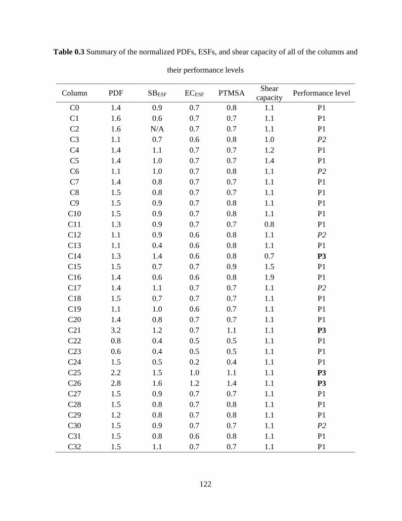
122

Table 0.3 Summary of the normalized PDFs, ESFs, and shear capacity of all of the columns and

their performance levels

Column PDF SBESF ECESF PTMSA Shear

capacity Performance level

C0 1.4 0.9 0.7 0.8 1.1 P1

C1 1.6 0.6 0.7 0.7 1.1 P1

C2 1.6 N/A 0.7 0.7 1.1 P1

C3 1.1 0.7 0.6 0.8 1.0 P2

C4 1.4 1.1 0.7 0.7 1.2 P1

C5 1.4 1.0 0.7 0.7 1.4 P1

C6 1.1 1.0 0.7 0.8 1.1 P2

C7 1.4 0.8 0.7 0.7 1.1 P1

C8 1.5 0.8 0.7 0.7 1.1 P1

C9 1.5 0.9 0.7 0.8 1.1 P1

C10 1.5 0.9 0.7 0.8 1.1 P1

C11 1.3 0.9 0.7 0.7 0.8 P1

C12 1.1 0.9 0.6 0.8 1.1 P2

C13 1.1 0.4 0.6 0.8 1.1 P1

C14 1.3 1.4 0.6 0.8 0.7 P3

C15 1.5 0.7 0.7 0.9 1.5 P1

C16 1.4 0.6 0.6 0.8 1.9 P1

C17 1.4 1.1 0.7 0.7 1.1 P2

C18 1.5 0.7 0.7 0.7 1.1 P1

C19 1.1 1.0 0.6 0.7 1.1 P1

C20 1.4 0.8 0.7 0.7 1.1 P1

C21 3.2 1.2 0.7 1.1 1.1 P3

C22 0.8 0.4 0.5 0.5 1.1 P1

C23 0.6 0.4 0.5 0.5 1.1 P1

C24 1.5 0.5 0.2 0.4 1.1 P1

C25 2.2 1.5 1.0 1.1 1.1 P3

C26 2.8 1.6 1.2 1.4 1.1 P3

C27 1.5 0.9 0.7 0.7 1.1 P1

C28 1.5 0.8 0.7 0.8 1.1 P1

C29 1.2 0.8 0.7 0.8 1.1 P1

C30 1.5 0.9 0.7 0.7 1.1 P2

C31 1.5 0.8 0.6 0.8 1.1 P1

C32 1.5 1.1 0.7 0.7 1.1 P1

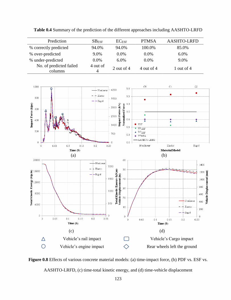
123

Table 0.4 Summary of the prediction of the different approaches including AASHTO-LRFD

Prediction SBESF ECESF PTMSA AASHTO-LRFD

% correctly predicted 94.0% 94.0% 100.0% 85.0%

% over-predicted 9.0% 0.0% 0.0% 6.0%

% under-predicted 0.0% 6.0% 0.0% 9.0%

No. of predicted failed

columns

4 out of

4 2 out of 4 4 out of 4 1 out of 4

(a) (b)

(c) (d)

Vehicle’s rail impact Vehicle’s Cargo impact

Vehicle’s engine impact Rear wheels left the ground

Figure 0.8 Effects of various concrete material models: (a) time-impact force, (b) PDF vs. ESF vs.

AASHTO-LRFD, (c) time-total kinetic energy, and (d) time-vehicle displacement

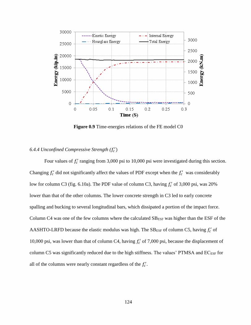
124

Figure 0.9 Time-energies relations of the FE model C0

6.4.4 Unconfined Compressive Strength (𝑓𝑐′)

Four values of 𝑓𝑐′ ranging from 3,000 psi to 10,000 psi were investigated during this section.

Changing 𝑓𝑐′ did not significantly affect the values of PDF except when the 𝑓𝑐

′ was considerably

low for column C3 (fig. 6.10a). The PDF value of column C3, having 𝑓𝑐′ of 3,000 psi, was 20%

lower than that of the other columns. The lower concrete strength in C3 led to early concrete

spalling and bucking to several longitudinal bars, which dissipated a portion of the impact force.

Column C4 was one of the few columns where the calculated SBESF was higher than the ESF of the

AASHTO-LRFD because the elastic modulus was high. The SBESF of column C5, having 𝑓𝑐′ of

10,000 psi, was lower than that of column C4, having 𝑓𝑐′ of 7,000 psi, because the displacement of

column C5 was significantly reduced due to the high stiffness. The values’ PTMSA and ECESF for

all of the columns were nearly constant regardless of the 𝑓𝑐′.

125

6.4.5 Strain Rate Effect

The PDF increased significantly when the strain rate effect was included (fig. 6.10b). The

PDF of column C0, which was modeled including the strain rate effect, was approximately 27%

higher than that of column C6, which was modeled excluding the strain rate effect. Including the

strain rate effect, the column’s strength and stiffness increased leading to higher dynamic forces.

However, this higher stiffness resulted in smaller SBESF because the column’s displacement

significantly reduced. There is no significant effect of strain rate effect on ECESF and PTMSA.

6.4.6 Percentage of Longitudinal Reinforcement

Three values of longitudinal reinforcement ratios ranging from 1% to 3% were investigated

during this section. In general, the PDF slightly increased when the percentage of longitudinal

reinforcement increased (fig. 6.10c). Tripling the percentage of longitudinal reinforcement

increased the PDF by 10% only. It increased because the column’s flexural strength and stiffness

slightly increased with increasing the flexural steel ratio. When the percentage of longitudinal

reinforcement increased, SBESF decreased while the ECESF and PTMSA were constant.

6.4.7 Hoop Reinforcement

Four volumetric hoop reinforcement ratios ranging from 0.54% (#[email protected] inch) to 0.17%

(#5@12 inch) were investigated during this section. The PDF decreased when the volume of hoop

reinforcement decreased leading to increasing concrete damage that dissipated a significant portion

of the impact energy (fig. 6.10d). The PDF decreased by 12% when the volume of hoop

reinforcement decreased by 67%. When the hoop reinforcement decreased, SBESF slightly increased

because the column’s displacement increased while the ECESF and PTMSA were constant.

mailto:#[email protected]

126

6.4.8 Column Span-to-Depth Ratio

Three values of column span-to-depth ratio ranging from 2.5 to 10 were investigated during

this section. The relationship between the PDF and the column’s span-to-depth ratio was nonlinear

(fig. 6.10e). The PDF of column C0, having span-to-depth ratio of 5, was higher than that of

columns C12 and C13, having span-to-depth ratios of 2.5 and 10, respectively. This was because

the column C12 had high local damaged buckling of several rebars leading to energy dissipation,

and column C13 had the lowest stiffness leading to energy dissipation through the high column’s

displacement.

The SBESF and ECESF were related, overall, nonlinearly to the span-to-depth ratio. The SBESF

of column C13 was significantly lower than the other columns because of its low column stiffness.

The PTMSA and ECESF are approximately constant regardless of the span-to-depth ratio.

6.4.9 Column Diameter

Four values of column’s diameter ranging from 4.0 ft to 7.0 ft were investigated during this

section. The PDF of all of the columns, except for Column C16, slightly increased when the

column diameter increased (fig. 6.10f). The PDF of the column C16, having a diameter of 7.0 ft,

was lower than that of the column C15, having a diameter of 6.0 ft because of the rebars’ buckling.

Additionally, column C14 of the diameter of 4.0 ft failed under the impact loading because of the

severe rebar buckling that occurred (fig. 6.11).

The SBESF tended to rapidly decrease when the column diameter increased, which

significantly increased column stiffness and significantly decreased the lateral displacement. The

SBESF was slightly higher than the PDF of column C14 having the lowest column diameter. This

column had high lateral displacement due to its small stiffness combined with relatively high PDF

leading to the highest SBESF. This was one of the few columns where SBESF exceeded that of

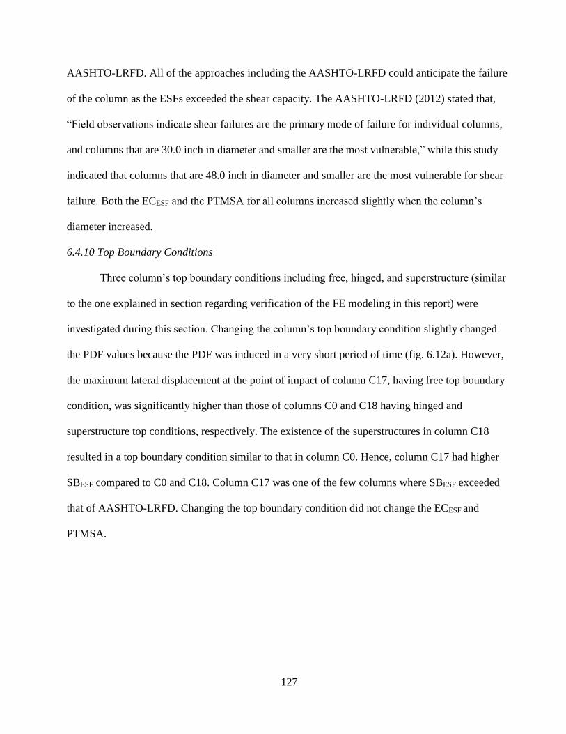
127

AASHTO-LRFD. All of the approaches including the AASHTO-LRFD could anticipate the failure

of the column as the ESFs exceeded the shear capacity. The AASHTO-LRFD (2012) stated that,

“Field observations indicate shear failures are the primary mode of failure for individual columns,

and columns that are 30.0 inch in diameter and smaller are the most vulnerable,” while this study

indicated that columns that are 48.0 inch in diameter and smaller are the most vulnerable for shear

failure. Both the ECESF and the PTMSA for all columns increased slightly when the column’s

diameter increased.

6.4.10 Top Boundary Conditions

Three column’s top boundary conditions including free, hinged, and superstructure (similar

to the one explained in section regarding verification of the FE modeling in this report) were

investigated during this section. Changing the column’s top boundary condition slightly changed

the PDF values because the PDF was induced in a very short period of time (fig. 6.12a). However,

the maximum lateral displacement at the point of impact of column C17, having free top boundary

condition, was significantly higher than those of columns C0 and C18 having hinged and

superstructure top conditions, respectively. The existence of the superstructures in column C18

resulted in a top boundary condition similar to that in column C0. Hence, column C17 had higher

SBESF compared to C0 and C18. Column C17 was one of the few columns where SBESF exceeded

that of AASHTO-LRFD. Changing the top boundary condition did not change the ECESF and

PTMSA.

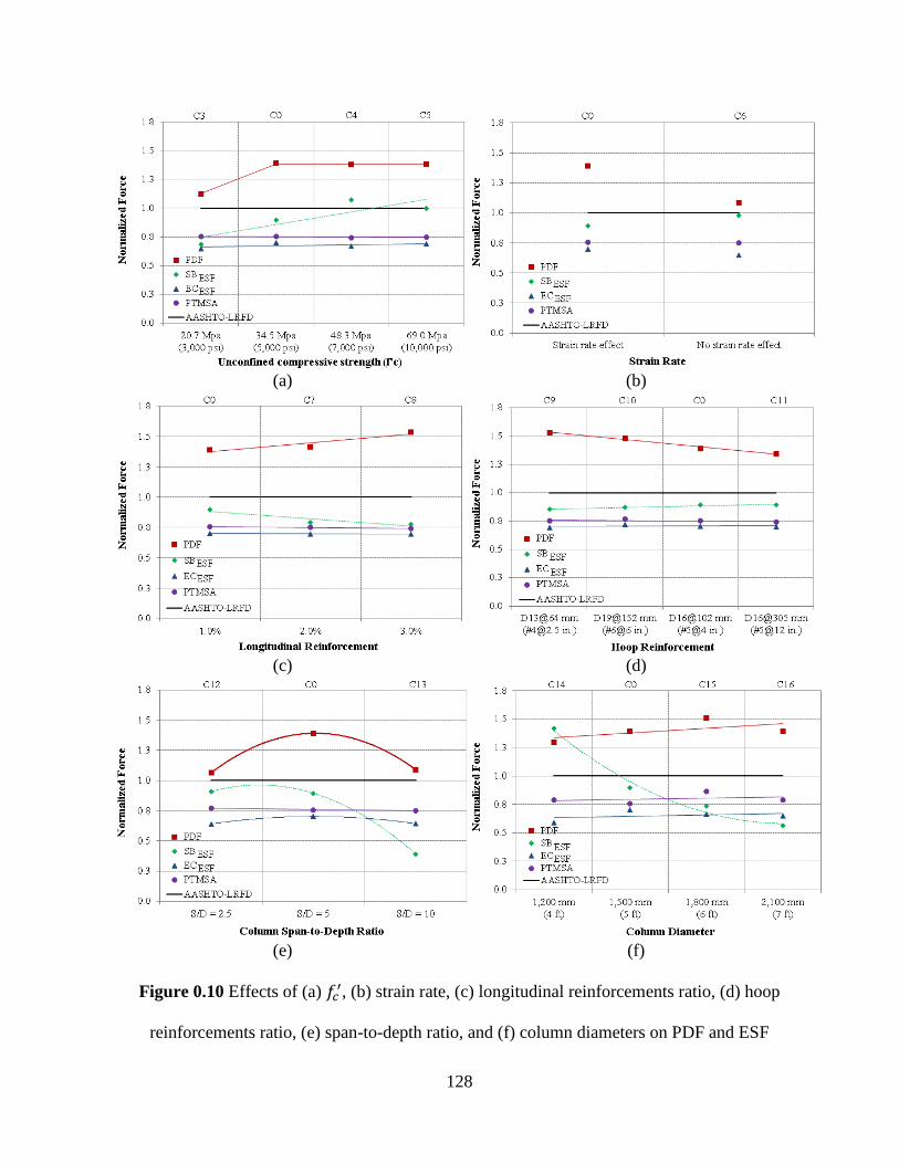
128

(a) (b)

(c) (d)

(e) (f)

Figure 0.10 Effects of (a) 𝑓𝑐′, (b) strain rate, (c) longitudinal reinforcements ratio, (d) hoop

reinforcements ratio, (e) span-to-depth ratio, and (f) column diameters on PDF and ESF

129

Figure 0.11 Buckling of rebars of column C14 having a diameter of 4 ft scaled 50 times

6.4.11 Axial Load Level

Three values of axial load level ranging from 0 to 10% of the column’s axial capacity (Po)

were investigated during this section. The PDF typically increased when the axial load level

increased (fig. 6.12b). Column C19, which sustained zero axial load, had a PDF that was

approximately 25% lower than that of column C20, which sustained an axial load that was 10% the

Po. The high axial compressive stresses on the column delayed the tension cracks due to the vehicle

impact and hence increased the column’s cracked stiffness leading to higher dynamic forces. The

PTMSA and ECESF are approximately constant regardless of the axial load level.

6.4.12 Vehicle Velocity

Four vehicle velocities ranging from 20 mph to 70 mph were investigated during this

section. The PDF tended to increase nonlinearly when the vehicle’s velocity increased (fig. 6.12c).

It is of interest that the increase in the PDF is not proportional to the square of the velocity as in the

case of elastic impact problems. Damage to the columns reduces the rate of increase in the PDF.

For example, the PDF increased by approximately 500% when the vehicle’s velocity increased

from 20 mph to 70 mph.

130

All of the ESFs approximately linearly increased as the vehicle velocity increased. PTMSA

and SBESF are the only approaches that the failure of column C21 having the vehicle’s velocity of

70 mph could be expected. However, AASHTO-LRFD and ECESF under-predicted the ESF of the

collision of vehicles moving at high speeds with the RC-columns.

6.4.13 Vehicle Mass

Four vehicle masses ranging from 4.4 kips to 65 kips were investigated during this section.

In general, both the PDF and ESF increased linearly when the vehicle’s mass increased (fig. 6.12d).

However, the rate of increase is slower than what is anticipated in elastic impact problems. For

example, the PDF increased by approximately 101% when the vehicle’s mass increased from 4.4

kips to 65 kips. The PDF almost did not change when the vehicle mass increased from 4.4 kips to

18 kips because the energy dissipation in the form of inelastic deformations, whether in the vehicle

or in the column, did not significantly change as the kinetic energy was not considerably high.

All approaches for calculating ESF resulted in higher values compared to that of AASHTO-

LRFD when the column collided with heavy vehicles of a weight more than 35 kips. PTMSA and

SBESF predicted the failure of the columns when they collided with heavy vehicles of a weight more

than 35 kips. However, the ECESF predicted only the column’s failure when the vehicle of a weight

of 65 kips collided with the column. AASHTO-LRFD under-predicted the columns’ failure when

they collided with heavy vehicles of a weight more than 35 kips.

6.4.14 Clear Zone Distance

Five clear zone distances ranging from zero to 30 ft were investigated during this section. In

general, the PDF decreased when the clear zone distance increased (fig. 6.12e). PTMSA and ECESF

are approximately constant regardless of the clear zone distance, while SBESF generally decreased

when the clear zone distance increased.

131

6.4.15 Soil Depth above the Top of the Column Footing

Three values of the soil depth above the top of the column footing ranging from 1.7 ft to 4.9

ft were investigated during this section. In general, the change in the soil depth above the column

footing did not significantly affect the PDF (fig. 6.12f). However, SBESF linearly increased when

the soil depth above the column footing increased. For large soil depth, the SBESF was 20% higher

than that of AASHTO-LRFD because the vehicle impact was closed to the middle of the column,

leading to high displacement. PTMSA and ECESF are approximately constant regardless of the soil

depth.

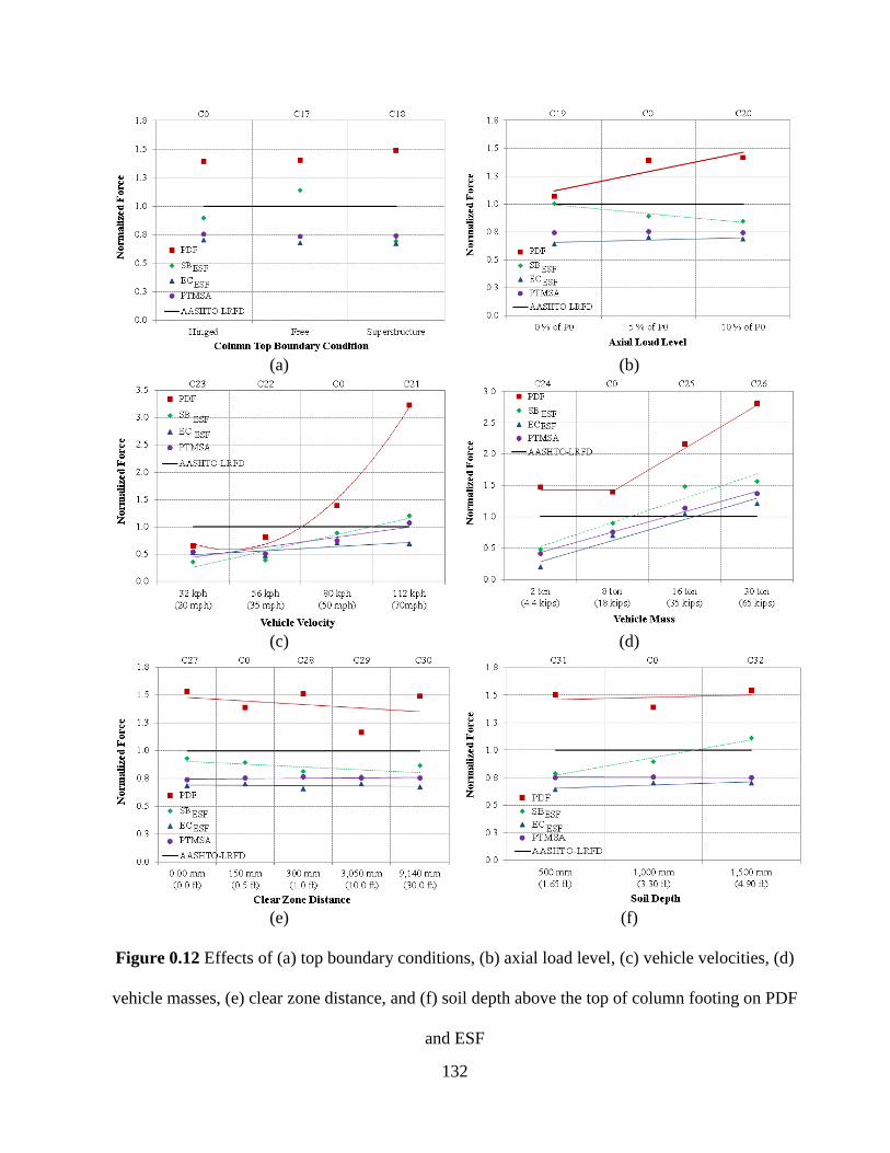
132

(a) (b)

(c) (d)

(e) (f)

Figure 0.12 Effects of (a) top boundary conditions, (b) axial load level, (c) vehicle velocities, (d)

vehicle masses, (e) clear zone distance, and (f) soil depth above the top of column footing on PDF

and ESF

133

6.5 Proposed Variable ESF for Adoption by AASHTO-LRFD

AASHTO-LRFD uses constant value for ESF regardless of vehicle and/or column

characteristics. However, all other approaches use variable ESF depending on the column and/or

vehicle characteristics. While the AASHTO-LRFD approach for ESF is quite simple, figs 6.7, 6.8,

and 6.9 as well as tables 6.3 and 6.4 showed that in some cases AASHTO-LRFD is quite

conservative and in other cases, such as those involving heavy trucks and high speeds, AASHTO-

LRFD under-predicts the impact loads. However, the other approaches require a cumbersome FE

analysis and iterative design. Therefore, having a simple equation to predict the ESF without a

cumbersome FE and iterative analysis would represent a significant improvement over the current

AASHTO-LRFD approach. Figures 6.11 and 6.12 reveal that vehicle mass and velocity are the

most influential parameters on the impact problems while the other parameters either have

insignificant effect or limited effects. Hence, it seems reasonable to develop a vehicle impact load

as a function of mass and velocity of the vehicle. This approach will allow Departments of

Transportation (DOTs) to design different bridge columns to different impact forces depending on

the anticipated truck loads and velocities. Vehicles’ information can be identified by the database of

roads’ survey that defines the mass and velocity of the frequent trucks on a specific road. Therefore,

the ESF of the impact should be classified by the type of road that the bridge pier serves. Since

PTMSA correctly predicted the performance of all the columns investigated in this study, it was

selected to be the basis for the newly developed equation. Based on the FE results of PTMSA of the

parametric study, and using CurveExpert Professional software and SAS software, a new equation

for estimating kinetic energy-based equivalent static force KEBESF is developed and presented in

equation 6.3 as shown below:

134

𝐾𝐸𝐵𝐸𝑆𝐹 = 2.1 √𝑚 𝑣𝑟2 = 3 √𝐾𝐸 (6.3)

where KEBESF = proposed ESF to AASHTO-LRFD (kip), m = the vehicle mass in kip, vr = the vehicle

velocity in mph, and KE = kinetic energy of the vehicle in kip.mph2.

The results of the proposed equations were compared with the FE results of PTMSA. The

ESFs of the additional fourteen columns that collided with SUT trucks of different masses ranging

from 18 kips to 90 kips were calculated and compared with the results of equation 6.3. Figure 6.13

illustrates the relation between the vehicle kinetic energy of the vehicles and normalized PTMSA as

well as between normalized KEBESF and the vehicle kinetic energy for all of the forty-seven

columns investigated in this study. As shown in the figure, up to KE of approximately 1,844 kip-ft,

AASHTO-LRFD over-predicated ESF. However, beyond that, AASHTO-LRFD is quite

conservative. In some cases, the RC-columns were subjected to impact loads that were almost

double that of the ESF of AASHTO-LRFD. Also shown in the figure are the upper and lower limits

referring to ± 10% of the KEBESF in order to visualize the error of equation 6.3 versus the PTMSA

results. The proposed equation KEBESF showed good agreement with averages, standard deviations,

and the coefficient of variation of 1.1, 8.7, and 8.2, respectively. Figure 6.15 illustrates the

normalized forces using the proposed equation 6.3 for the investigated columns compared to the

columns’ shear capacity and AASHTO-LRFD ESF. The figure showed that the KEBESF could

predict the columns’ performance by 100% and 4 out of 4 of the failed columns.

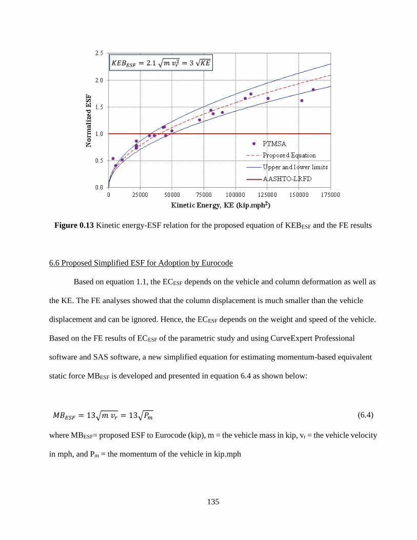
135

Figure 0.13 Kinetic energy-ESF relation for the proposed equation of KEBESF and the FE results

6.6 Proposed Simplified ESF for Adoption by Eurocode

Based on equation 1.1, the ECESF depends on the vehicle and column deformation as well as

the KE. The FE analyses showed that the column displacement is much smaller than the vehicle

displacement and can be ignored. Hence, the ECESF depends on the weight and speed of the vehicle.

Based on the FE results of ECESF of the parametric study and using CurveExpert Professional

software and SAS software, a new simplified equation for estimating momentum-based equivalent

static force MBESF is developed and presented in equation 6.4 as shown below:

𝑀𝐵𝐸𝑆𝐹 = 13√𝑚 𝑣𝑟 = 13√𝑃𝑚 (6.4)

where MBESF= proposed ESF to Eurocode (kip), m = the vehicle mass in kip, vr = the vehicle velocity

in mph, and Pm = the momentum of the vehicle in kip.mph

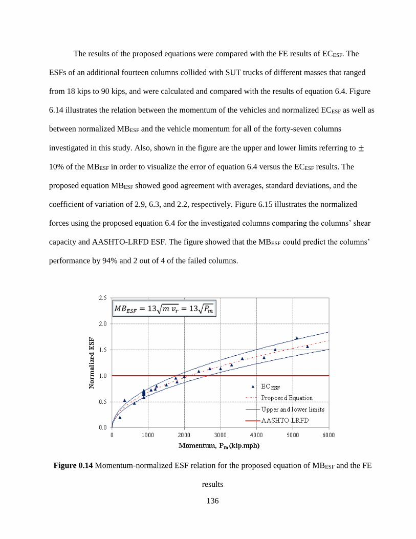
136

The results of the proposed equations were compared with the FE results of ECESF. The

ESFs of an additional fourteen columns collided with SUT trucks of different masses that ranged

from 18 kips to 90 kips, and were calculated and compared with the results of equation 6.4. Figure

6.14 illustrates the relation between the momentum of the vehicles and normalized ECESF as well as

between normalized MBESF and the vehicle momentum for all of the forty-seven columns

investigated in this study. Also, shown in the figure are the upper and lower limits referring to ±

10% of the MBESF in order to visualize the error of equation 6.4 versus the ECESF results. The

proposed equation MBESF showed good agreement with averages, standard deviations, and the

coefficient of variation of 2.9, 6.3, and 2.2, respectively. Figure 6.15 illustrates the normalized

forces using the proposed equation 6.4 for the investigated columns comparing the columns’ shear

capacity and AASHTO-LRFD ESF. The figure showed that the MBESF could predict the columns’

performance by 94% and 2 out of 4 of the failed columns.

Figure 0.14 Momentum-normalized ESF relation for the proposed equation of MBESF and the FE

results

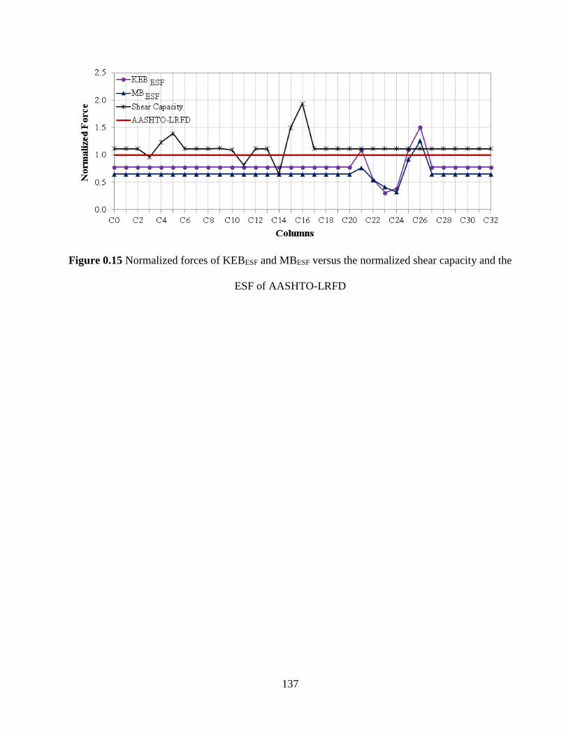
137

Figure 0.15 Normalized forces of KEBESF and MBESF versus the normalized shear capacity and the

ESF of AASHTO-LRFD

138

Chapter 7 Analysis of Vehicle Collision with HC-FCS Bridge Columns

7.1 Research Significance

Several studies investigated the behavior of the reinforced concrete bridge columns under

vehicle impact; however, very few studies investigated the behavior of other types of bridge

columns under vehicle impact. This manuscript used detailed finite element analyses to investigate

the behavior of the hollow-core FRP-concrete-steel (HC-FCS) columns under vehicle impact.

Comparisons between the ESF of the AASHTO-LRFD (600 kips) and the calculated ESF using

different approaches are presented as well.

7.2 Parametric Study

A parametric study was conducted to numerically investigate the behavior of the HC-FCS

columns under a vehicle collision. Eleven columns were explored, named C0 to C10. Column C0

was used as a reference column. LS-DYNA was used to examine four different parameters. These

parameters included:

Vehicle velocity (vr) ranging from 20 mph to 70 mph

Vehicle mass (m) ranging from 4.4 kips to 65 kips

Unconfined compressive strength (𝑓𝑐′) ranging from 3,000 psi to 10,000 psi

Material strain rate (SR; considered and not considered)

7.3 FE Modelling of HC-FCSs

Figures 7.1a and 7.1b illustrate the FE modeling details of the HC-FCS columns. The inner

steel tube was extended inside the footing using an embedded length (Le), while the FRP tube was

stopped at the top of the footing. The steel tube was hollow inside. All of the columns did not

include any shear or flexure reinforcement except the steel tube. The columns investigated in this

study were supported on a concrete footing that had fixed boundary condition at its bottom. All of

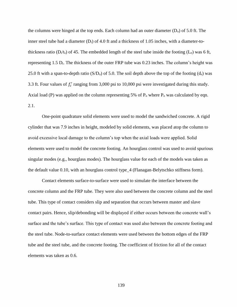
139

the columns were hinged at the top ends. Each column had an outer diameter (Do) of 5.0 ft. The

inner steel tube had a diameter (Di) of 4.0 ft and a thickness of 1.05 inches, with a diameter-to-

thickness ratio (Di/ts) of 45. The embedded length of the steel tube inside the footing (Le) was 6 ft,

representing 1.5 Di. The thickness of the outer FRP tube was 0.23 inches. The column’s height was

25.0 ft with a span-to-depth ratio (S/Do) of 5.0. The soil depth above the top of the footing (ds) was

3.3 ft. Four values of 𝑓𝑐′ ranging from 3,000 psi to 10,000 psi were investigated during this study.

Axial load (P) was applied on the column representing 5% of Po where Po was calculated by eqn.

2.1.

One-point quadrature solid elements were used to model the sandwiched concrete. A rigid

cylinder that was 7.9 inches in height, modeled by solid elements, was placed atop the column to

avoid excessive local damage to the column’s top when the axial loads were applied. Solid

elements were used to model the concrete footing. An hourglass control was used to avoid spurious

singular modes (e.g., hourglass modes). The hourglass value for each of the models was taken as

the default value 0.10, with an hourglass control type_4 (Flanagan-Belytschko stiffness form).

Contact elements surface-to-surface were used to simulate the interface between the

concrete column and the FRP tube. They were also used between the concrete column and the steel

tube. This type of contact considers slip and separation that occurs between master and slave

contact pairs. Hence, slip/debonding will be displayed if either occurs between the concrete wall’s

surface and the tube’s surface. This type of contact was used also between the concrete footing and

the steel tube. Node-to-surface contact elements were used between the bottom edges of the FRP

tube and the steel tube, and the concrete footing. The coefficient of friction for all of the contact

elements was taken as 0.6.

140

A nonlinear concrete material model (mat72RIII) was used for all columns and footings in

this study. An elasto-plastic constitutive model, mat003-plastic_kinamatic, was used for the steel

tube. The following parameters were needed to define this material model: the elastic modulus (E),

the yield stress, and Poisson’s ratio. These parameters were assigned the following values: 29,000

ksi, 60,900 psi, and 0.30, respectively (Caltrans 2006). To consider strain rate effect, Cowper-

Symonds’s model was adopted. The strain rate effect was considered for all of the columns except

column C10.

The FRP material used was modeled as an orthotropic material using “002-

orthotropic_elastic” material. This material is defined by several engineering constants: elastic

modulus (E), shear modulus (G), and Poisson’s ratio (PR), in the three principle axes (a, b, and c).

The fiber orientation is defined by a vector. The following characteristics, based on the

manufacturer “Grace Composites and FRP Bridge Drain Pipe,” were implemented in the FE. The

elastic modulus in the hoop direction (Ea), shear modulus in the transverse direction (Gab), and

Poisson’s ratio of the FRP tube were 3,020 ksi, 406 ksi, and 0.35, respectively. The failure criterion

for the FRP, defined as “000-add_erosion,” was assigned the ultimate strain of FRP in “EFFEPS”

card. The ultimate tensile strain in the hoop direction was 0.013. To consider strain rate effect, the

Gama and Gillespie (2011) model was adopted.

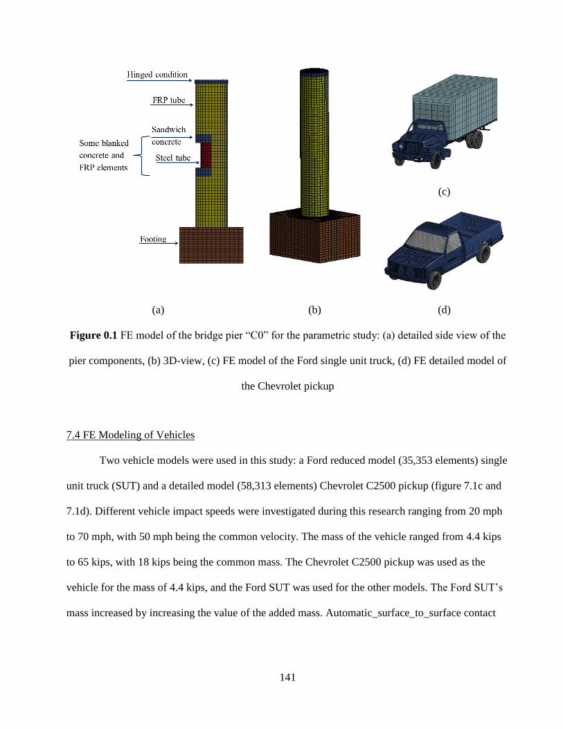
141

(c)

(a) (b) (d)

Figure 0.1 FE model of the bridge pier “C0” for the parametric study: (a) detailed side view of the

pier components, (b) 3D-view, (c) FE model of the Ford single unit truck, (d) FE detailed model of

the Chevrolet pickup

7.4 FE Modeling of Vehicles

Two vehicle models were used in this study: a Ford reduced model (35,353 elements) single

unit truck (SUT) and a detailed model (58,313 elements) Chevrolet C2500 pickup (figure 7.1c and

7.1d). Different vehicle impact speeds were investigated during this research ranging from 20 mph

to 70 mph, with 50 mph being the common velocity. The mass of the vehicle ranged from 4.4 kips

to 65 kips, with 18 kips being the common mass. The Chevrolet C2500 pickup was used as the

vehicle for the mass of 4.4 kips, and the Ford SUT was used for the other models. The Ford SUT’s

mass increased by increasing the value of the added mass. Automatic_surface_to_surface contact

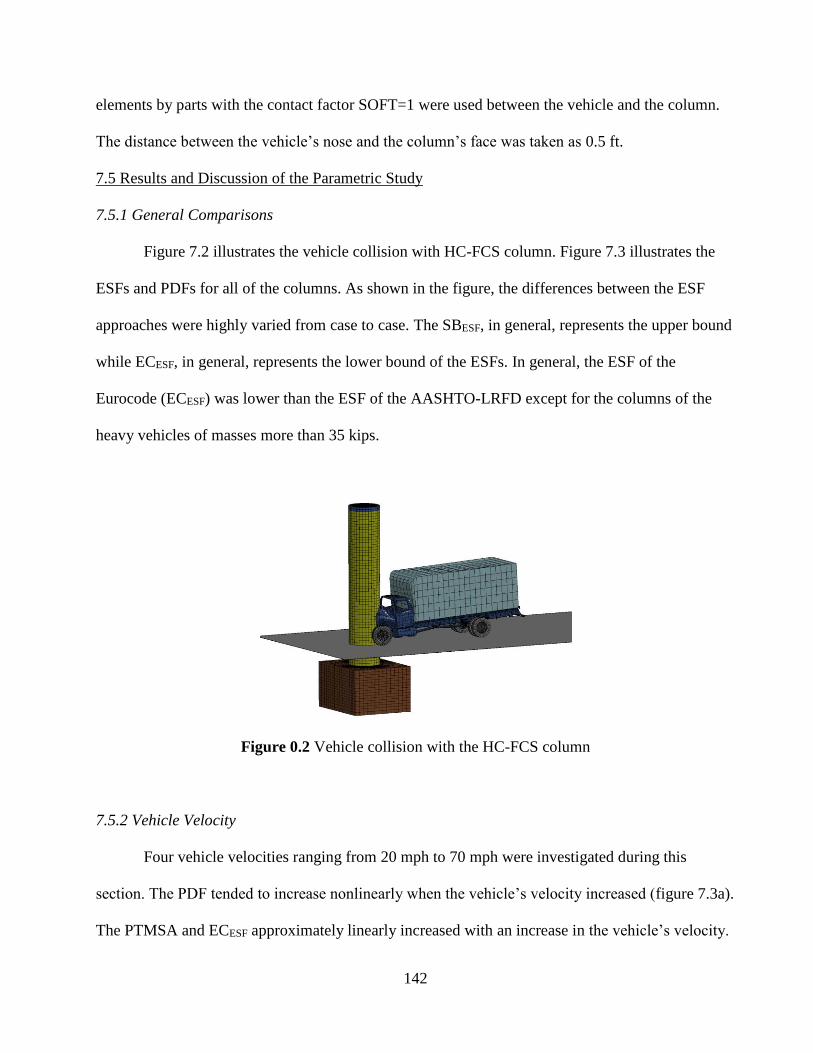
142

elements by parts with the contact factor SOFT=1 were used between the vehicle and the column.

The distance between the vehicle’s nose and the column’s face was taken as 0.5 ft.

7.5 Results and Discussion of the Parametric Study

7.5.1 General Comparisons

Figure 7.2 illustrates the vehicle collision with HC-FCS column. Figure 7.3 illustrates the

ESFs and PDFs for all of the columns. As shown in the figure, the differences between the ESF

approaches were highly varied from case to case. The SBESF, in general, represents the upper bound

while ECESF, in general, represents the lower bound of the ESFs. In general, the ESF of the

Eurocode (ECESF) was lower than the ESF of the AASHTO-LRFD except for the columns of the

heavy vehicles of masses more than 35 kips.

Figure 0.2 Vehicle collision with the HC-FCS column

7.5.2 Vehicle Velocity

Four vehicle velocities ranging from 20 mph to 70 mph were investigated during this

section. The PDF tended to increase nonlinearly when the vehicle’s velocity increased (figure 7.3a).

The PTMSA and ECESF approximately linearly increased with an increase in the vehicle’s velocity.

143

However, the SBESF increased nonlinearly when the vehicle’s velocity increased. All of the ESFs

were lower than or approximately equal to the ESF of the AASHTO-LRFD.

7.5.3 Vehicle Mass

Four vehicle masses ranging from 4.4 kips to 65 kips were investigated during this section.

In general, both the PDF and ESF increased linearly when the vehicle’s mass increased (figure

7.3b). The PDF almost did not change when the vehicle mass increased from 4.4 kips to 18 kips

because the energy dissipation in the form of inelastic deformations, whether in the vehicle or in the

column, did not significantly change as the kinetic energy was not considerably high. All

approaches for calculating ESF resulted in higher values compared to that of tAASHTO-LRFD

when the column collided with heavy vehicles that weighed more than 35 kips.

7.5.4 Unconfined Compressive Strength (𝑓𝑐′)

Four values of 𝑓𝑐′ ranging from 3,000 psi to 10,000 psi were investigated during this section.

The PDF slightly increased when the 𝑓𝑐′ increased (figure 7.3c). The PTMSA and the ECESF for all

of the columns were nearly constant regardless of the 𝑓𝑐′. However, the SBESF slightly increased

when the 𝑓𝑐′ increased because of the increase of column’s stiffness as the concrete modulus of

elasticity increased.

7.5.5 Strain Rate Effect

The PDF slightly increased when the strain rate effect was included (figure 7.3d). Including

the strain rate effect, the column’s strength and stiffness increased, which led to higher dynamic

forces. However, this higher stiffness resulted in a smaller SBESF because the column’s

displacement significantly reduced. There is no significant effect of strain rate effect on ECESF and

PTMSA.

144

(a) (b)

(c) (d)

Figure 0.3 Effects of (a) vehicle velocity, (b) vehicle mass, (c) fc′, and (d) strain rate on PDF and

ESF

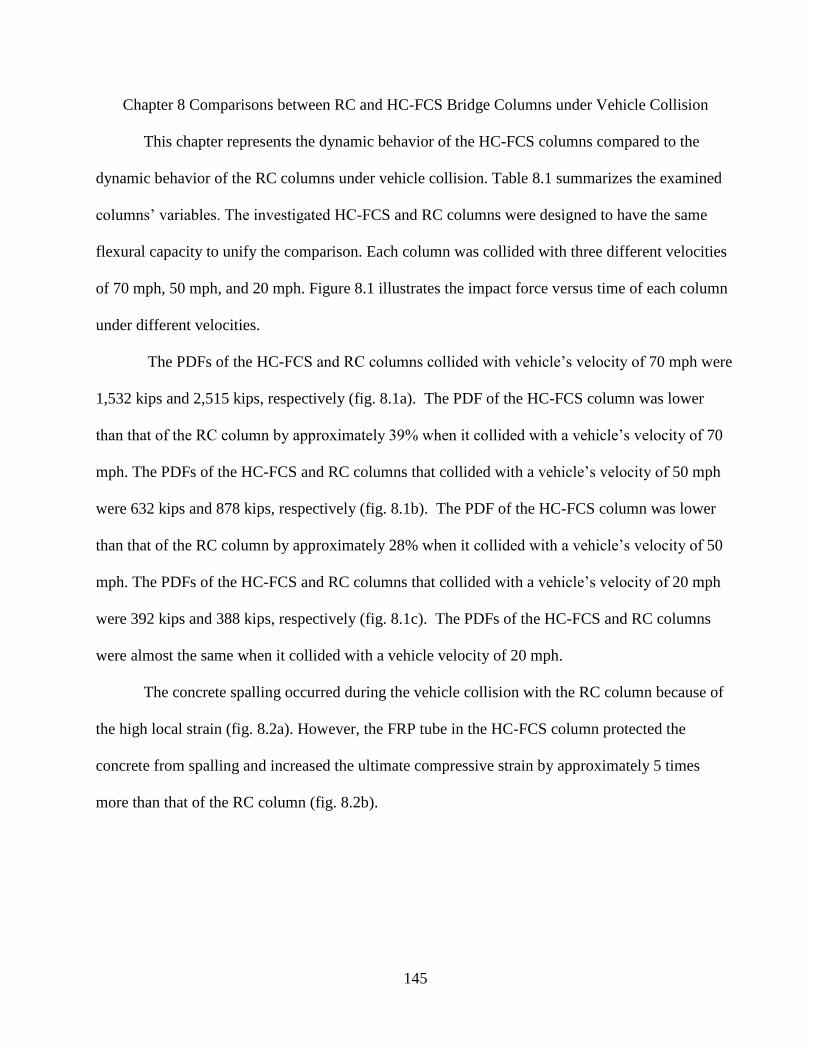
145

Chapter 8 Comparisons between RC and HC-FCS Bridge Columns under Vehicle Collision

This chapter represents the dynamic behavior of the HC-FCS columns compared to the

dynamic behavior of the RC columns under vehicle collision. Table 8.1 summarizes the examined

columns’ variables. The investigated HC-FCS and RC columns were designed to have the same

flexural capacity to unify the comparison. Each column was collided with three different velocities

of 70 mph, 50 mph, and 20 mph. Figure 8.1 illustrates the impact force versus time of each column

under different velocities.

The PDFs of the HC-FCS and RC columns collided with vehicle’s velocity of 70 mph were

1,532 kips and 2,515 kips, respectively (fig. 8.1a). The PDF of the HC-FCS column was lower

than that of the RC column by approximately 39% when it collided with a vehicle’s velocity of 70

mph. The PDFs of the HC-FCS and RC columns that collided with a vehicle’s velocity of 50 mph

were 632 kips and 878 kips, respectively (fig. 8.1b). The PDF of the HC-FCS column was lower

than that of the RC column by approximately 28% when it collided with a vehicle’s velocity of 50

mph. The PDFs of the HC-FCS and RC columns that collided with a vehicle’s velocity of 20 mph

were 392 kips and 388 kips, respectively (fig. 8.1c). The PDFs of the HC-FCS and RC columns

were almost the same when it collided with a vehicle velocity of 20 mph.

The concrete spalling occurred during the vehicle collision with the RC column because of

the high local strain (fig. 8.2a). However, the FRP tube in the HC-FCS column protected the

concrete from spalling and increased the ultimate compressive strain by approximately 5 times

more than that of the RC column (fig. 8.2b).

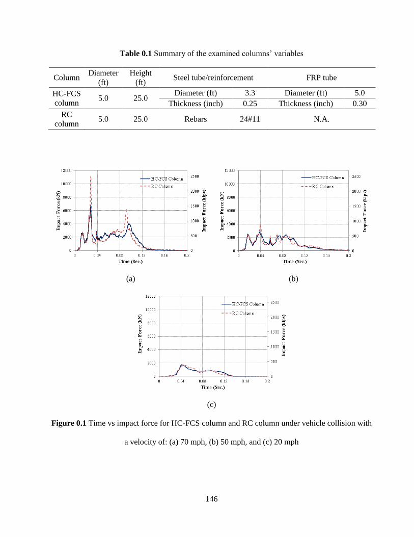
146

Table 0.1 Summary of the examined columns’ variables

Column Diameter

(ft)

Height

(ft) Steel tube/reinforcement FRP tube

HC-FCS

column 5.0 25.0

Diameter (ft) 3.3 Diameter (ft) 5.0

Thickness (inch) 0.25 Thickness (inch) 0.30

RC

column 5.0 25.0 Rebars 24#11 N.A.

(a) (b)

(c)

Figure 0.1 Time vs impact force for HC-FCS column and RC column under vehicle collision with

a velocity of: (a) 70 mph, (b) 50 mph, and (c) 20 mph

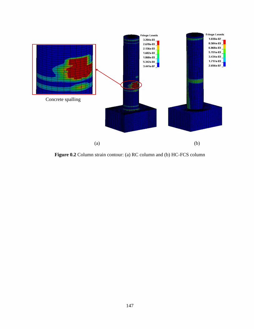
147

(a) (b)

Figure 0.2 Column strain contour: (a) RC column and (b) HC-FCS column

Concrete spalling

148

Chapter 9 Conclusions and Future Work

9.1 Conclusions

This report presented the behavior of HC-FCS columns under axial, combined axial-

flexural, and vehicle collision loading. The effects of using different steel tube diameter-to-

thickness ratio (D/t), outer FRP tubes with different orientations, and different concrete wall

thickness, on the behavior of HC-FCS columns under axial loading were investigated. HC-FCS

columns with wet lay-up FRP tubes having ± 45° exhibited a higher level of axial strain capacity

than that of the unconfined concrete. However, the increase in strength due to confinement was

minimal.

HC-FCS columns with wet lay-up FRP tubes having ± 45° and 0° (hybrid FRP)

exhibited high axial strengths and strains. The failure of the HC-FCS columns with hybrid FRP

tubes consisted of two stages. The first stage was the rupture of the unidirectional FRP (outer

tube), and then the second stage was the reorientation of the angle-plied FRP exhibiting high

axial strains. HC-FCS columns having steel tubes of high D/t ratio was not effective in confining

the concrete shell. The local buckling of the steel tube affected the overall hoop strain of the FRP

tube.

Four large scale columns, a conventionally reinforced concrete (RC) column having a

solid cross section, and three HC-FCS columns were investigated during this study. Each column

had an outer diameter of 24 inches and a column’s aspect ratio, height-to-diameter ratio, of 4.0.

The steel tube was extended inside the footing with an embedded length of 1.6 times the steel

tube diameter. Additionally, the FRP tube only confined the concrete wall thickness and

truncated at the top of the footing level. The hollow steel tube was the only reinforcement for

shear and flexure inside the HC-FCS column. The HC-FCS column exhibited high lateral drift

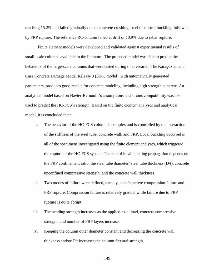
149

reaching 15.2% and failed gradually due to concrete crushing, steel tube local buckling, followed

by FRP rupture. The reference RC-column failed at drift of 10.9% due to rebar rupture.

Finite element models were developed and validated against experimental results of

small-scale columns available in the literature. The proposed model was able to predict the

behaviors of the large-scale columns that were tested during this research. The Karagozian and

Case Concrete Damage Model Release 3 (K&C model), with automatically generated

parameters, produces good results for concrete modeling, including high strength concrete. An

analytical model based on Navier-Bernoulli’s assumptions and strains compatibility was also

used to predict the HC-FCS’s strength. Based on the finite element analyses and analytical

model, it is concluded that:

i. The behavior of the HC-FCS column is complex and is controlled by the interaction

of the stiffness of the steel tube, concrete wall, and FRP. Local buckling occurred in

all of the specimens investigated using the finite element analyses, which triggered

the rupture of the HC-FCS system. The rate of local buckling propagation depends on

the FRP confinement ratio, the steel tube diameter/ steel tube thickness (D/t), concrete

unconfined compressive strength, and the concrete wall thickness.

ii. Two modes of failure were defined, namely, steel/concrete compression failure and

FRP rupture. Compression failure is relatively gradual while failure due to FRP

rupture is quite abrupt.

iii. The bending strength increases as the applied axial load, concrete compressive

strength, and number of FRP layers increase.

iv. Keeping the column outer diameter constant and decreasing the concrete wall

thickness and/or D/t increases the column flexural strength.

150

v. The columns’ drifts increase as the applied axial load, unconfined concrete

compressive strength, and steel tube D/t decrease. The columns’ drifts increase as the

FRP layers increase.

vi. The flexural strength slightly increases as the number of FRP layers increases

regardless of the steel tube D/t ratio within the range of the parameters investigated in

this study.

A detailed description of finite element modeling of vehicle collision with RC bridge

columns using LS-DYNA software was presented in this report. Evaluation of the peak dynamic

force (PDF) and the equivalent static force (ESF) through an extensive parametric study were

conducted. The extensive parametric study investigated the effects of concrete material model,

maximum unconfined concrete compressive stress (𝑓𝑐′), material strain rate, percentage of

longitudinal reinforcement, hoop reinforcement, column span-to-depth ratio, column diameter,

the top boundary conditions, axial load level, vehicle’s velocity, vehicle’s mass, clear zone

distance, and soil depth above the top of the column footing on the PDF and ESF. Three

approaches were considered during the course of this research to investigate the ESF. In the first

approach, SBESF, the ESF was defined as the force needed to produce the same maximum

displacement by a collision event at the point of impact. In the second approach, ECESF, the ESF

was calculated by Eurocode. In the third approach, PTMSA, the ESF was defined as the peak of

the 25 millisecond moving average. This study revealed the following findings:

The AASHTO-LRFD was found to be non-conservative when the column was collided

with heavy vehicles of a weight more than 35 kips or high speed vehicle more than 70

mph. In another terms, the AASHTO-LRFD nonconservative for KE higher than 1,800

151

kip-ft. The AASHTO-LRFD predicted 85% of the columns’ performance, and predicted

only 1 out of 4 of the failed columns.

A new equation for estimating the ESF based on the vehicle’s mass and velocity,

(𝐾𝐸𝐵𝐸𝑆𝐹 = 33√𝑚 𝑣𝑟2 ) with more than 90% accuracy, was developed. This approach

will allow Departments of Transportation (DOTs) to design different bridge columns to

different impact forces depending on the anticipated truck loads and velocities.

This report simplified the Eurocode equation for estimating the ESF based on the

vehicle’s mass and velocity (𝑀𝐵𝐸𝑆𝐹 = 130√𝑚 𝑣𝑟 ) with more than 90% accuracy.

Approximately 12% of the columns failed while 15% and 73% of the columns were

assigned to performance levels P2 and P1, respectively.

PTMSA approach was the best approach for predicting the columns’ performance by

100% and 4 out of 4 of the failed columns, while SBESF predicted 94% of the columns’

performance and 4 out of 4 of the failed columns. Furthermore, ECESF predicted 94% of

the columns’ performance and 2 out of 4 of the failed columns.

This study indicated that columns that are 48.0 inches in diameter and smaller are the

most vulnerable for shear failure contradicting the AASHTO-LRFD (2012) which states

that columns that are 30.0 inches in diameter and smaller are the most vulnerable.

Different approaches predict different vehicle impact force values, and there is no

consensus among researchers on the best approach. For a given column and impact

scenario, the difference between the estimated maximum and minimum impact force

(ESF) ranged from 7% to 140%.

The SBESF generally represents the upper bound for 73% of the impact cases while ECESF

represents the lower bound for 85% of the columns.

152

The impact demand forces according to SBESF and PTMSA exceeded the ESF of the

AASHTO-LRFD by 27% and 9%, respectively. The ESF of the Eurocode (ECESF) was

typically lower than the ESF of the AASHTO-LRFD.

Generally, the PDF increases when the longitudinal reinforcement ratio, hoop

reinforcement volumetric ratio, column diameter, axial load level, vehicle velocity, and

vehicle mass increase, and when the strain rate effect is considered. Additionally, it

decreases when the damage of the column and the clear zone distance increase. However,

it is not affected by changing 𝑓𝑐′, column top boundary condition, and soil depth.

The relation between the PDF and the column’s span-to-depth ratio was nonlinear.

A detailed description of finite element modeling of vehicle collision with HC-FCS bridge

columns using LS-DYNA software was presented in this report. Evaluation of the peak dynamic

force (PDF) and the equivalent static force (ESF) through a parametric study were conducted.

The parametric study investigated the effects of the vehicle velocity, vehicle mass, unconfined

concrete compressive stress (𝑓𝑐′), and material strain rate were carried out. The three approaches

of estimating the ESF were investigated. This study revealed the following findings:

The AASHTO-LRFD was found to be non-conservative when the column collided with

heavy vehicles that weighed more than 35 kips.

The difference between the ESF calculated by the different approaches highly varied.

The SBESF generally represents the upper bound of the ESF while ECESF represents the

lower bound.

The ESF of the Eurocode (ECESF) was typically lower than the ESF of the AASHTO-

LRFD.

153

Generally, the PDF increases when the 𝑓𝑐′, vehicle velocity and vehicle mass increase,

and when the strain rate effect is considered.

The dynamic behavior of the HC-FCS columns was compared to the dynamic behavior of

the RC columns under vehicle collision. Each column collided with three different velocities of

70 mph, 50 mph, and 20 mph. The PDFs were calculated and compared for each case. The PDF

values of the HC-FCS columns were lower than those of the RC column by approximately 28% -

39% when they collided with vehicles having velocities ranging from 50 mph to 70 mph. The

vehicles mass was 18 kips. The PDFs of the HC-FCS and RC columns were approximately equal

when they collided with a vehicle having a velocity of 20 mph. Concrete spalling occurred

during the vehicle collision with the RC column because of high local strains. However, the FRP

tube in the HC-FCS column protected the concrete from spalling and increased the ultimate

compressive strain by approximately 5 times more than that of the RC column.

9.2 Future Work

While extensive research was carried out during the current project, including testing on

small-scale cylinders, large-scale testing, analytical modeling, and finite element modeling under

lateral and vehicle impact, there remain a few issues that need to be addressed before field

implementation of HC-FCS. Future work is required to address the following issues:

Shear strength of HC-FCS. For short columns, there will be an interaction between the

shear and flexural strength of the columns, moreover, how much of a contribution steel

and FRP have on the shear strength.

Determination of the required steel tube embedded length to achieve full fixation and

avoid pull-out of the column from footing. The embedded length needs to be a function

in tube diameter, yield strength, thickness, and concrete strength.

154

Develop and test a cap-beam column connection.

Torsion strength of the column. Skew and curved bridges may induce torsion on

columns. The contribution of concrete, FRP tube, and steel tube to torsional resistance

need to be determined.

Durability studies of the steel encased into the concrete and FRP tube is required.

Optimization of the construction cost of the HC-FCS column. Cost analysis and

comparisons with conventional concrete columns need to be carried out. Then, the price

need to be optimized.

155

References

AASHTO, (2012), AASHTO-LRFD Bridge Design Specifications – Customary US Units, sixth

edition, Washington, DC.

AASHTO, (2010), AASHTO-LRFD Bridge Design Specifications – Customary US Units, fifth

edition, Washington, DC.

Abdelkarim, O. and ElGawady, M. (2014a). “Behavior of Hybrid FRP-Concrete-Steel Double-Skin

Tubes Subjected to Cyclic Axial Compression.” Structures Congress 2014: pp. 1002-1013.

Abdelkarim, O. and ElGawady, M. (2014b). "Analytical and Finite-Element Modeling of FRP-

Concrete-Steel Double-Skin Tubular Columns." J. Bridge Eng., 10.1061/(ASCE)BE.1943-

5592.0000700 , B4014005.

Abdelkarim, O., Geni, A., Anumolu, S., and ElGawady, M. (2015). “Seismic Behavior of Hollow-

Core FRP-Concrete-Steel Bridge columns.” ASCE Structures Congress, pp. 585-596.

Abdelkarim, O. and ElGawady, M. (2015). “Impact Analysis of Vehicle Collision with Reinforced

Concrete Bridge Columns.” Transportation Research Board (TRB) conference, Washington Dc,

15-4461.

Agrawal, A. K., Liu, G., and Alampalli, S. (2013). “Effects of Truck Impacts on Bridge Piers.”

Advanced Materials Research, 639-640, pp.13-25.

Agrawal, A.K. (2011). “Bridge Vehicle Impact Assessment: Final Report.” University

Transportation Research Center and New York State Department of Transportation.

Alias, M.N. and R. Brown, 1992, Corosion, 48: 373-378.

American Concrete Institute (ACI) Committee 318 (2011). “Building Code Requirements for

Structural Concrete (ACI 318-11) and Commentary (318R-11).” ACI, Farmington Hills, Mich.,

509 pp.

American Concrete Institute (ACI) Committee 440 (2008). “Guide for the Design and Construction

of Externally Bonded FRP Systems for Strengthening Concrete Structures.” ACI 440.2R-08,

2008, Farmington Hills, MI.

American Concrete Institute (ACI) Committee 440 (2007). “Report on Fiber-Reinforced Polymer

(FRP) Reinforcement for Concrete Structures.” ACI 440R-07, 2007, Farmington Hills, MI.

Amir Fam, Andrew Kong, and Mark F. Green. (2008) “Effects of freezing and thawing cycles and

sustained loading on compressive strength of precast concrete composite piles.” PCI journal, V.

53, No. 1, January–February 2008, pp. 109–120.

http://ascelibrary.org/doi/abs/10.1061/%28ASCE%29BE.1943-5592.0000700

http://ascelibrary.org/doi/abs/10.1061/%28ASCE%29BE.1943-5592.0000700

156

Ashbee K and Wyatt R. (1969), “Water damage in glass fibre/resin composites.” Proceedings of the

Royal Society of London. Series A, Mathematical and Physical Sciences, Vol. 312, No. 1511

(Sep. 30, 1969), pp. 553-564.

Ashbee, K. H. G. 1989. Fundamental Principles of Fiber Reinforced Composites, Lancaster, PA:

Technomic Publishing CO. Inc.

ASTM Standard A1067, 2012, "Test Coupons for Steel Castings," ASTM International, West

Conshohocken, PA, 2012, 10.1520/A1067_A1067M-12A.

ASTM Standard D3039, 2008, Standard Test Method for Tensile Properties of Polymer Matrix

Composite Materials," ASTM International, West Conshohocken, PA, 2008,

10.1520/D3039_D3039M-08.

Au, C. and Buyukozturk, O. (2005). ”Effect of Fiber Orientation and Ply Mix on Fiber Reinforced

Polymer-Confined Concrete.” J. Compos. Constr., 9(5), 397–407.

Bala, S. (2001). “Contact Modeling in LS-DYNA.” Livermore Software Technology Corporation.

Balazs, G. and Borosnyoi, A. (2001). “Long-Term Behavior of FRP.” Composites in Construction:

pp. 84-91. doi: 10.1061/40596(264)10.

Benmokrane, B., Wang, P., Ton-That, T., Rahman, H., and Robert, J. (2002). “Durability of Glass

Fiber-Reinforced Polymer Reinforcing Bars in Concrete Environment.” J. Compos.

Constr., 6(3), 143–153.

Bischoff, P.H., Perry, S.H., “Compressive Behavior of Concrete at High Strain Rates.” Materials

and Structures, Vol. 24, 1991, pp. 425-450.

Bowles, J. (1988) “Foundation Analysis and Design.” McGraw-Hill Inc., United States of America,

1004 pp.

Bradshaw RD, Brinson LC. (1997). “Physical aging in polymer composites: an analysis and method

for time aging time superposition.” Polymer Engineering & Science, Volume 37, Issue 1, pp.

31–44, January 1997.

Buth, C. E., Williams, W. F., Brackin, M. S., Lord, D., Geedipally, S. R., and Abu-Odeh, A. Y.

(2010). “Analysis of Large Truck Collisions with Bridge Piers: Phase 1.” Texas Department of

Transportation Research and Technology Implementation Office, 9-4973-1.

Buth, C. E., Brackin, M. S., Williams, W. F., and Fry, G.T. (2011). “Collision Loads On Bridge

Piers: Phase 2.” Texas Department of Transportation Research and Technology Implementation

Office, Report 9-4973-2.

California Department of Transportation. (2006). “Seismic Design Criteria”. California Department

of Transportation, Rev. 1.4.

157

Campbell, J.D. (1954). “The yield of mild steel under impact loading.” Journal of the Mechanics

and Physics of Solids, 3, 54-62.

Charles, RJ. (1959), “The strength of silicate glasses and some crystalline oxides [chapter 12].”

Cheikh, A.Al. and Murat, M. (1988). “Kinetics of Non-Congruent Dissolution of E-Glass Fiber in

Saturated Calcium Hydroxide Solution.” Cement and Concrete Research, Volume 18, Issue 6,

November 1988, Pages 943–950.

Chen Y, Davalos JF, Ray I, Kim HY. (2007). “Accelerated aging tests for evaluation of durability

performance of FRP reinforcing bars reinforcing bars for concrete structures” Composite

Structures, Volume 78, Issue 1, March 2007, pp. 101–111.

Chin JW, Aouadi K, Nguyen T. (1997) “Effects of environmental exposure on fiber-reinforced

plastic (FRP) materials used in construction.” J Compos Technol Res 1997; 19(4):205–13.

Comité Euro-International du Béton. (1993). “CEB-FIP Model Code 1990.” Redwood Books,

Trowbridge, Wiltshire, UK.

Cowper, G. R. and Symonds, P. S. (1957). “Strain Hardening and Strain Rate Effects in Impact

Loading of Cantilever Beams.” Brown University, App. Math. Report No. 28.

D’Almieda. J. R. M. 1991. Composite Materials, 15: 117-132.

Dawood, H., ElGawady, M. (2013). “Performance-based seismic design of unbonded precast post-

tensioned concrete filled GFRP tube piers” Composites Part B: Engineering, Volume 44, Issue

1, Pages 357-367.

Dawood, H., ElGawady, M., and Hewes, J. (2012). “Behavior of Segmental Precast Post-Tensioned

Bridge Piers under Lateral Loads.” ASCE Journal of Bridge Engineering, Vol. 17, No. 5, pp.

735-746.

Earl, J.S. and Shenoi, R.A. (2004). “Hygrothermal ageing effects on FRP laminate and structural

foam materials.” Composites Part A: Applied Science and Manufacturing. Volume 35, Issue 11,

November 2004, pp. 1237-1247.

ElGawady, M. and Dawood, H. (2012). “Analysis of segmental piers consisted of concrete filled

FRP tubes.” Engineering Structures, Vol. 38, pp. 142-152.

ElGawady, M. and Sha’lan, A. (2011). ”Seismic Behavior of Self-Centering Precast Segmental

Bridge Bents.” J. Bridge Eng., 16(3), 328–339.

ElGawady, M., Booker, A., and Dawood, H. (2010). ”Seismic Behavior of Posttensioned Concrete-

Filled Fiber Tubes.” J. Compos. Constr., 14(5), 616–628.

http://www.sciencedirect.com/science/article/pii/0022509654900393

http://www.scopus.com/source/sourceInfo.url?sourceId=28635&origin=resultslist

http://www.sciencedirect.com/science/journal/01410296

158

El-Tawil, S., Severino, E., and Fonseca, P. (2005). “Vehicle Collision with Bridge Piers.” J. Bridge

Eng., 10(3), 345-353.

Eurocode 1: Actions on structures – Part 1-1: General actions – Densities, self-weight, imposed

loads for buildings, Final Draft prEN 1991-1-1, October 2002.

Evans, K. E. B. D. Caddock and K. L. Ainsworth. 1988, Journal of Material Science 23: 2926-

2930.

Fabio Nardone, Marco Di Ludovico, Francisco J. De Caso y Basalo, Andrea Prota, Antonio Nanni,

(2012) “Tensile behavior of epoxy based FRP composites under extreme service conditions”

Composites Part B: Engineering Volume 43, Issue 3, April 2012, pp. 1468-1474.

Fakharifar, M., Sharbatdar, M. K., Lin, Z., Dalvand, A., Sivandi-Pour, A., & Chen, G. (2014).

Seismic performance and global ductility of RC frames rehabilitated with retrofitted joints by

CFRP laminates. Earthquake Engineering and Engineering Vibration, 13(1), 59-73. DOI:

10.1007/s11803-014-0212-6.

Fam, A. Z.; Schnerch, D.; and Rizkalla, S. H., 2002, “Moisture Effect on Durability of Concrete-

Filled GFRP Tubular Piles.” NCSU-CFL Report No. 02-04, Constructed Facilities Laboratory,

North Carolina State University, Raleigh, NC.

Fouche, P., Bruneau, M. (2010). “Non-Linear Analysis of Multi-Hazard Performance of Cylindrical

Concrete Filled Steel Tubes Bridge Piers.” Proceedings of 8th International Conference on

Short and Medium Span Bridges, Canada.

Francesco Micelli and Antonio Nanni, “Durability of FRP rods for concrete structures.”

Construction and Building Materials 18 (2004) pp. 491–503.

Fu, H.C., Erki, M.A., Seckin, M., “Review of Effects of Loading Rate on Reinforced Concrete,”

Journal of Stru. Eng., Vol. 117, No. 12, December 1991, pp. 3660-3679.

Gama, BA., Gillespie, JW. (2011). “Finite element modeling of impact, damage evolution and

penetration of thick-section composites.” International Journal of Impact Engineering, 38 (4),

pp. 181-197.

Gentry, T.R., Bank, L.C., Barkatt, A., and Prian, L. (1998). “Accelerated Test Methods to

Determine the Long-Term Behavior of Composite Highway Structures Subject to

Environmental Loading.” Journal of Composites Technology & Research, JCTRER, Vol. 20,

No.1, January 1998, pp.38-50.

Hajjar J. (2000). “Concrete-filled steel tube columns under earthquake loads.” Structural

Engineering and Materials; 2(1):72–82.

Han, L.H., Tao, Z., Liao, F.Y., and Xu, Y. (2010). “Tests on Cyclic Performance of FRP-Concrete-

Steel Double-Skin Tubular Columns.” Thin-Walled Structures, 4, 430-439.

http://www.sciencedirect.com/science/article/pii/S0734743X1000196X


159

Han L.H., Huang H., Tao Z. and Zhao X.L. (2006). “Concrete-filled double skin steel tubular

(CFDST) beam-columns subjected to cyclic bending”, Engineering Structures, Vol.28, No.12,

1698–714.

Harik, I., Shaaban, A., Gesund, H., Valli, G., and Wang, S. (1990). ”United States Bridge Failures,

1951–1988.” J. Perform. Constr. Facil., 4(4), 272–277.

Holmes, T.M., Leatherman, G.L. and El-Korchi, T. (1991). “Alkali-Resistant Oxynitride Glasses.”

Journal of Material Research, Vol. 6, No. 1, Jan 1991, pp. 152-158.

Huang, H., Han, L. H., Zhao, X. (2013). “Investigation on concrete filled double skin steel tubes

(CFDSTs) under pure torsion” Journal of Constructional Steel Research, Volume 90, 221-234.

Joannie W. Chin, Khaled Aouadi, Michael R. Haight, William L. Hughes, and Tinh Nguyen,

(2001), “Effects of Water, Salt Solution and Simulated Concrete Pore Solution on the Properties

of Composite Matrix Resins Used in Civil Engineering Applications.” Polymer Composites,

April 2001, vol. 22, no. 22, pp. 282-298.

Jones, F. R. J. W. Rock and A. R. Wheatley. 1983, Journal of Composite Materials, 14: 213-232.

Karbhari, V.M., Murphy K., and Zhang, S. (2002). “Effect of Concrete Based Alkali Solutions on

Short-Term Durability of E-Glass/Vinylester Composites.” Journal of Composite Materials,

September 2002, vol. 36 no. 17, pp. 2101-2121.

Kootsookos, A, Mouritz, A.P, St John, N.A. (2001). “Comparison of the Seawater Durability of

Carbon- and Glass-Polymer composites.” ICCM-13, 2001, Beijing, China.

Lawrence C. Bank, T. Russell Gentry, Benjamin P. Thompson and Jeffrey S. Russell. (2003). “A

model specification for FRP composites for civil engineering structures.” Construction and

Building Materials 17(2003), pp. 405–437.

Li, W., Han,L. H., Chan, T. (2014a). “Tensile behaviour of concrete-filled double-skin steel tubular

members” Journal of Constructional Steel Research, Volume 99, 35-46.

Li, W., Han,L. H., Chan, T. (2014b). “Numerical investigation on the performance of concrete-

filled double-skin steel tubular members under tension” Thin-Walled Structures, Volume 79,

108-118.

Lima Sobrinho, Ledjane; Ferreira, Marysilvia and Bastian, Fernando Luiz. (2009). “The effects of

water absorption on an ester vinyl resin system.” Mat. Res. 2009, vol.12, n.3, pp. 353-361.

LS-DYNA. (2007). “Keyword user’s manual.” Livermore Software Technology Corporation, CA.

http://www.sciencedirect.com/science/article/pii/S0143974X13002289

http://www.sciencedirect.com/science/article/pii/S0143974X13002289

160

Lu, H., Zhao, X., Han, L. H. (2010). “Testing of self-consolidating concrete-filled double skin

tubular stub columns exposed to fire” Journal of Constructional Steel Research, Volume 66,

Issues 8–9, 1069-1080.

Kansas Department of transportation. (2013). “Bridge LRFD Design Manual.”

Malvar, L. J. and Ross, C. A. (1998). “Review of Strain Rate Effects for Concrete in Tension.” ACI

Materials Journal, 95, 735-739.

Malvar, L., Crawford, J., Wesevich, J., and Simons, D. (1997). “A plasticity concrete material

model for DYNA3D.” Int. J. Impact Eng., 19(9–10), 847–873.

Mathieu Robert and Brahim Benmokrane (2013), “Combined effects of saline solution and moist

concrete on long-term durability of GFRP reinforcing bars.” Construction and Building

Materials. Volume 38, January 2013, pp. 274-284.

Mathieu Robert and Amir Fam, (2012), “Long-Term Performance of GFRP Tubes Filled with

Concrete and Subjected to Salt Solution.” J. Compos. Constr., 16(2), 217–224.

McBagonluri, F., Garcia, K., Hayes, M., Verghese, K.N.E., Lesko, J.J. (2000). “Characterization of

fatigue and combined environment on durability performance of glass/vinyl ester composite for

infrastructure applications.” International Journal of Fatigue, Volume 22, Issue 1, January 2000,

pp. 53–64.

McGrath, J.J. (2013). “Replacement of Missouri Route M Overpass Creamed by Freight-Train

Crash in Scott County Estimated to Cost about $3 Million: Accident is the Third Railroad

Mishap in Four Months in Rockview- May 26, 2013” International Business times,

http://www.ibtimes.com/replacement-missouri-route-m-overpass-creamed-freight-train-crash-

scott-county-estimated-cost-about, Accessed by July, 2014.

Mehta, K.P., Monteiro, P.J.M. (2006). “CONCRETE: Microstructure, Properties, and Materials”

3rd Edition, McGraw-Hill Inc., United States of America, 660 pp.

Micelli, F., and Myers, J.J. (2008), “Durability of FRP-confined concrete”. Proceedings of the ICE-

Construction Materials, Volume 161, Issue 4, 01 November 2008, pp. 173-185.

Miguel A. Pando, Carl D. Ealy, George M. Filz, J.J. Lesko, and E.J. Hoppe, (2006), “A Laboratory

and Field Study of Composite Piles for Bridge Substructures”. Report No. FHWA-HRT-04-

043.

Miguel Pando, Jack Lesko, Amir Fam, and Sami Rizkalla. (2002). “Moisture Effect on Durability

of Axially Loaded Concrete-Filled Tubular FRP Piles.” 2nd Int. Conf. on Durability of FRP

Composites in Construction, CDCC 2002, Sherbrooke, May 29-31, pp. 25-37.

Mohan, P., Marzougui, D., Kan, C. (2003). “Validation of a Single Unit Truck Model for Roadside

Hardware Impacts.” NCAC, The George Washington University.




http://www.ibtimes.com/replacement-missouri-route-m-overpass-creamed-freight-train-crash-scott-county-estimated-cost-about

http://www.ibtimes.com/replacement-missouri-route-m-overpass-creamed-freight-train-crash-scott-county-estimated-cost-about

161

Montague, P., (1978). “Experimental behavior of double-skinned, composite, circular cylindrical-

shells under external-pressure”. Journal of Mechanical Engineering Science, 20(1), pp. 21–34.

Moon, J., Lehman, D., Roeder, C., and Lee, H. (2013). ”Strength of Circular Concrete-Filled Tubes

with and without Internal Reinforcement under Combined Loading.” J. Structural Engineering,

139(12).

Moore, M. A. and H. H. Epps, 1992. Journal of Testing and Evaluation, 20(2): 139-143.

Ozbakkaloglu, T. and Idris, Y. (2014). ”Seismic Behavior of FRP-High-Strength Concrete–Steel

Double-Skin Tubular Columns.” J. Struct. Eng., 140(6), 04014019.

Ozbakkaloglu, T. and Fanggi, B. (2013). "Axial Compressive Behavior of FRP-Concrete-Steel

Double-Skin Tubular Columns Made of Normal- and High-Strength Concrete." J. Compos.

Constr., 10.1061/(ASCE)CC.1943-5614.0000401 , 04013027.

Phani, K. K. and Bose, N. R. (1987), “Temperature Dependence of Hydrothermal Ageing of CSM-

Laminate During Water Immersion.” Composites Science and Technology, Volume 29, Issue 2,

1987, pp. 79–87.

Piyush K. Dutta and David Hui, (1996), “Low-temperature and freeze-thaw durability of thick

composites.” Composites Part B: Engineering. Volume 27, Issues 3–4, 1996, pp. 371-379.

Rivera, J. and Karbhari, V. M. (2001), “Characterization of Sub-Zero Response of Vinylester FRP

in Civil Infrastructure Renewal.” The Eleventh International Offshore and Polar Engineering

Conference, 17-22, June 2001, Stavanger, Norway.

Robert, M., Wang, P., Cousin, P., and Benmokrane, B. (2010). “Temperature as an Accelerating

Factor for Long-Term Durability Testing of FRPs: Should There Be Any Limitations?” J.

Compos. Constr., 14(4), 361–367.

Ryu, D., Wijeyewickrema, A., ElGawady, M., and Madurapperuma, M. (2014). "Effects of Tendon

Spacing on In-Plane Behavior of Post-Tensioned Masonry Walls." J. Struct. Eng., 140(4),

04013096.

Sachin Kshirsagar, Roberto A. Lopez-Anido, and Rakesh K. Gupta, (2000), “Environmental Aging

of Fiber-Reinforced Polymer-Wrapped Concrete Cylinders.” ACI Material Journal, Volume 97,

Issue 6, pp. 703-712.

Shakir-Khalil, H., and Illouli, S. 1987. “Composite columns of concentric steel tubes.” Proc., Conf.

on the Design and Construction of Non-Conventional Structures, Vol. 1, London, pp. 73–82.

Sharma, H., Hurlebaus, S., Gardoni, P. (2012). “Performance-based response evaluation of

reinforced concrete columns subject to vehicle impact.” Inter. Journal of Impact Eng., (43), 52-

62.

http://ascelibrary.org/doi/abs/10.1061/%28ASCE%29CC.1943-5614.0000401

162

Shin, M. and Andrawes, B. (2010). “Experimental Investigation of Actively Confined Concrete

Using ShapeMemory Alloys”. J. Eng. Struct. 32:3, 656-664.

Siddhwartha Mandal, Andrew Hoskin, and Amir Fam. (2005). “Influence of Concrete Strength on

Confinement Effectiveness of Fiber-Reinforced Polymer Circular Jackets.” ACI Structural

Journal; May 2005, Vol. 102 Issue 3, p383.

Sierakowsi, R. L. and Chaturved, S. K. (1997). “Dynamic Loading and Characterization of Fiber-

Reinforced Composites,” John Wiley & Sons, Inc., New York, USA.

Silva, M., Cidade, M., Biscaia, H., and Marreiros, R. (2014). "Composites and FRP-Strengthened

Beams Subjected to Dry/Wet and Salt Fog Cycles." J. Mater. Civ. Eng., 10.1061/(ASCE), 2014,

MT.1943-5533.0001008 , 04014092.

Soles CL, Chang FT, Bolan BA, Hristov HA, Gidley DW, Yee AF. (1998). “Contributions of the

nanovoid structure to the moisture absorption properties of epoxy resins.” Journal of Polymer

Science Part B: Polymer Physics. Volume 36, Issue 17, pp. 3035–3048, December 1998.

Tannous FE, Saadatmanesh H. (1998). “Environmental effects on the mechanical properties of E-

glass FRP rebars.” ACI Materials Journal, Volume 95, Issue 2, pp. 87-100.

Teng, J. G., Yu, T., Wong, Y. L., and Dong, S. L. (2007). “Hybrid FRP concrete-steel tubular

columns: Concept and behavior.” Constr. Build. Mater., 21(4), 846–854.

Teng, J.G., Yu, T., Wong, Y.L., and Dong, S.L. (2005). “Innovative FRP-Steel-Concrete Hybrid

Columns.” Advances in Steel Structures, 1, 545-554.

Teng, J.G., Yu, T., and Wong, Y.L. (2004). “Behavior of Hybrid FRP-Concrete-Steel Double-Skin

Tubular Columns.” Proc. 2nd Int. Conf. on FRP Composites in Civil Engineering, Adelaide,

Australia, 811-818.

Thilakarathna, H.M.I., Thambiratnam, D.P., Dhanasekar, M., Perera, N. (2010). “Numerical

simulation of axially loaded concrete columns under transverse impact and vulnerability

assessment.” Inter. Journal of Impact Eng., (37), 1100-1112.

Tucker, W. C. and R. Brown. 1989. Journal of Composite Materials, 23: 787-797.

Underwood, J. H. and A. A. Kapusta. 1991. Journal of Composites Technology and Research, 13:

179-182.

Wassim Naguib and Amir Mirmiran. (2002). “Time-Dependent Behavior of Fiber-Reinforced

Polymer Confined Concrete Columns under Axial Loads.” ACI Structural Journal, V. 99, No. 2,

March-April 2002.

163

Williams, M.S., “Modeling of Local Impact Effects on Plain and Reinforced Concrete.” ACI

Structural Journal, Vol. 91, No. 2, March-April 1994, pp. 178-187.

Wolff, E. G. 1993, Sample Journal, 29(3):11-19.

Wong, Y. L., Yu, T., Teng, J. G., and Dong, S. L. (2008). “Behavior of FRP-confined concrete in

annular section columns.” Compos. B Eng., 39(3), 451–466.

Yagishita F, Kitoh H, Sugimoto M, Tanihira T, Sonoda K. (2000). “Double-skin composite tubular

columns subjected cyclic horizontal force and constant axial force.” Proceedings of the Sixth

ASCCS Conference, Los Angeles, USA, March 22–24, pp. 497–503.

Yan, X. and Yali, S. (2012). ”Impact Behaviors of CFT and CFRP Confined CFT Stub

Columns.” J. Compos. Constr., 16(6), 662–670.

Yilmaz, V.T. (1992). “Chemical attack on alkali-resistant glass fibers in a hydrating cement matrix:

characterization of corrosion products.” Journal of Non-Crystalline Solids, Volume 151, Issue

3, 2 December 1992, pp. 236–244.

Yu, T., Cao, Y., Zhang, B. & Teng, J. G. (2012). Hybrid FRP-concrete-steel double-skin tubular

columns: Cyclic axial compression tests. 6th International Conference on FRP Composites in

Civil Engineering (pp. 1-8).

Yu, T., Teng, J., and Wong, Y. (2010). ”Stress-Strain Behavior of Concrete in Hybrid FRP-

Concrete-Steel Double-Skin Tubular Columns.” J. Struct. Eng., 136(4), 379–389.

Yu, T., Wong, Y., Teng, J., Dong, S., and Lam, E. (2006). ”Flexural Behavior of Hybrid FRP-

Concrete-Steel Double-Skin Tubular Members.” J. Compos. Constr., 10(5), 443–452.

Yu, T., Wong, Y.L., Teng, J.G., and Dong, S.L., (2004). “Structural behavior of hybrid FRP-

concrete-steel double-skin tubular columns.” ANCER Annual Meeting: Networking of Young

Earthquake Engineering Researchers and Professionals, Honolulu, Hawaii.

Zaouk, A., Bedewi N.E., Kan, C.D., Marzougui, D. (1996). ”Validation of a Non-Linear Finite

Element Vehicle Model Using Multiple Impact Data.” International Mechanical Engineering

Congress and Exposition, Atlanta, GA.

Zaouk, A. K., Bedewi, N. E., Kan, C. D., and Marzoughi, D. (1996). “Evaluation of a Multi-

purpose Pick-up Truck Model Using Full Scale Crash Data with Application to Highway

Barrier Impact.” 29th Inter. Sym. on Auto. Tech. and Auto., Florence, Italy.

Zhang, B., Teng, J. G. and Yu, T. (2012). “Behaviour of hybrid double-skin tubular columns

subjected to combined axial compression and cyclic lateral loading.” Sixth International

Conference on FRP Composites in Civil Engineering (pp. 1-7). Rome, Italy.

164

Zhao, X., Bai, Y., Al-Mahaidi, R., and Rizkalla, S. (2014). ”Effect of Dynamic Loading and

Environmental Conditions on the Bond between CFRP and Steel: State-of-the-Art Review”. J.

Compos. Constr. 18, Special Issue: 10th Anniversary of IIFC, A4013005. 2014.

Zhu, Z., Ahmad, I., and Mirmiran, A. (2006). “Seismic performance of concrete-filled FRP tube

columns for bridge substructure.” J. Bridge Eng., 11(3), 359–370.

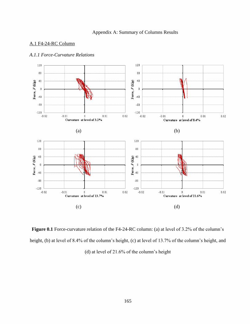
165

Appendix A: Summary of Columns Results

A.1 F4-24-RC Column

A.1.1 Force-Curvature Relations

(a) (b)

(c) (d)

Figure 0.1 Force-curvature relation of the F4-24-RC column: (a) at level of 3.2% of the column’s


(d) at level of 21.6% of the column’s height

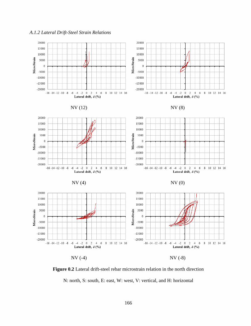
166

A.1.2 Lateral Drift-Steel Strain Relations

NV (12) NV (8)

NV (4) NV (0)

NV (-4) NV (-8)

Figure 0.2 Lateral drift-steel rebar microstrain relation in the north direction

N: north, S: south, E: east, W: west, V: vertical, and H: horizontal

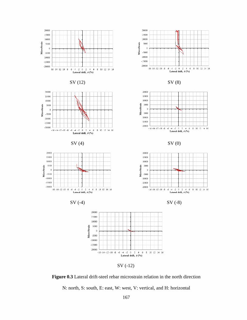
167

SV (12) SV (8)

SV (4) SV (0)

SV (-4) SV (-8)

SV (-12)

Figure 0.3 Lateral drift-steel rebar microstrain relation in the north direction


168

A.2 F4-24-E324 column


(a) (b)

(c) (d)

Figure 0.4 Force-curvature relation the F4-24-E324 column: (a) at level of 3.2% of the column’s


(d) at level of 21.6% of the column’s height

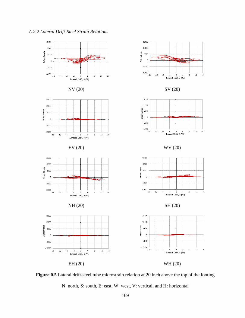
169


NV (20) SV (20)

EV (20) WV (20)

NH (20) SH (20)

EH (20) WH (20)

Figure 0.5 Lateral drift-steel tube microstrain relation at 20 inch above the top of the footing


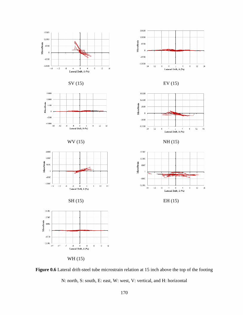
170

SV (15) EV (15)

WV (15) NH (15)

SH (15) EH (15)

WH (15)



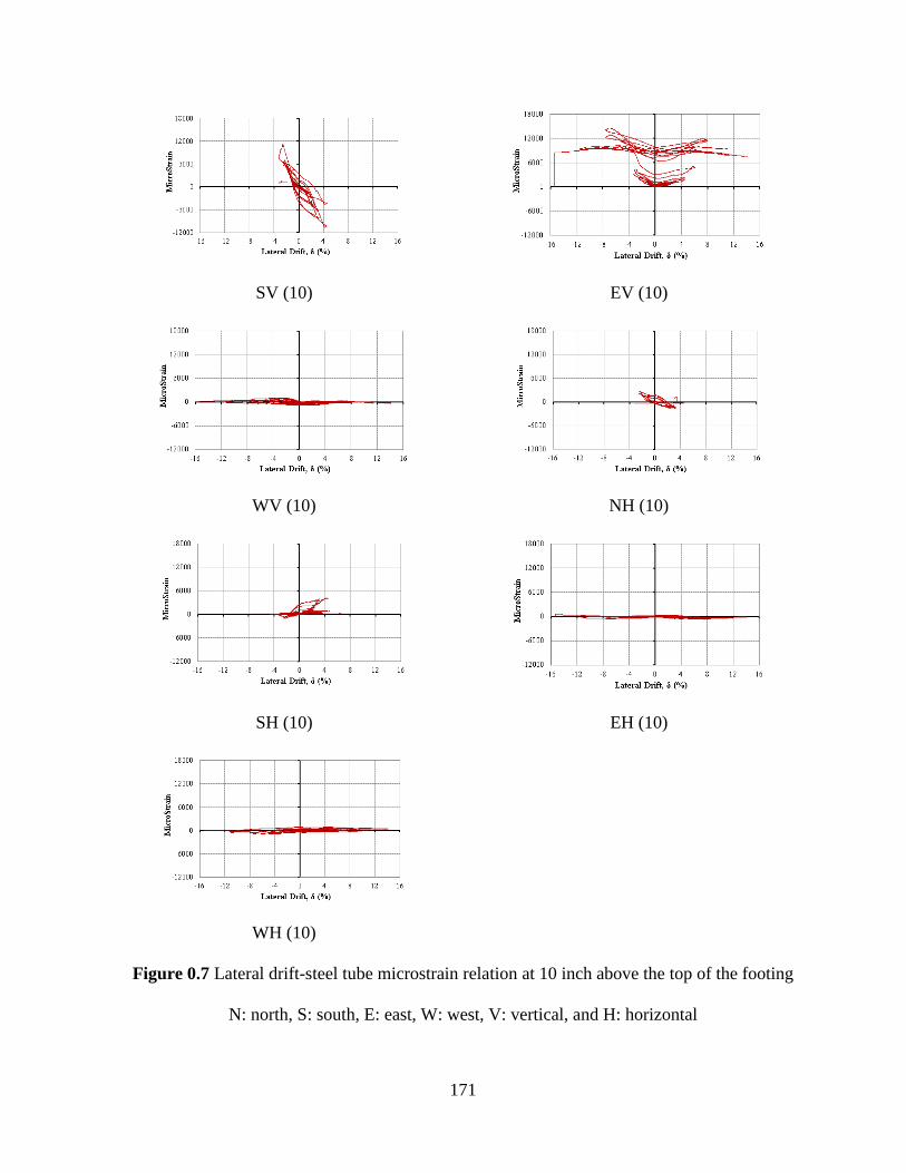
171

SV (10) EV (10)

WV (10) NH (10)

SH (10) EH (10)

WH (10)



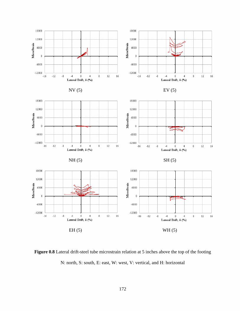
172

NV (5) EV (5)

NH (5) SH (5)

EH (5) WH (5)

Figure 0.8 Lateral drift-steel tube microstrain relation at 5 inches above the top of the footing


173

NV (0) SV (0)

EV (0) SH (0)

Figure 0.9 Lateral drift-steel tube microstrain relation at the level of the top of the footing


174

NV (-5) SV (-5)

EV (-5) WV (-5)

NH (-5) EH (-5)

Figure 0.10 Lateral drift-steel tube microstrain relation at 5 inch below the top of the footing


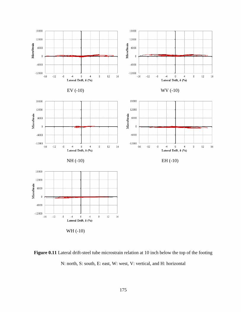
175

EV (-10) WV (-10)

NH (-10) EH (-10)

WH (-10)



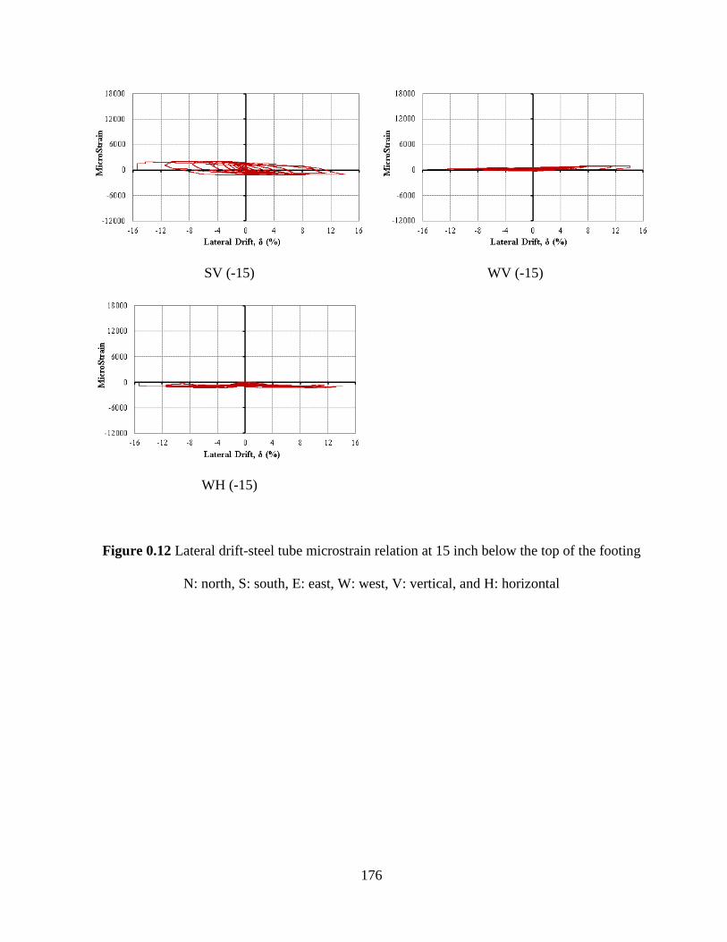
176

SV (-15) WV (-15)

WH (-15)



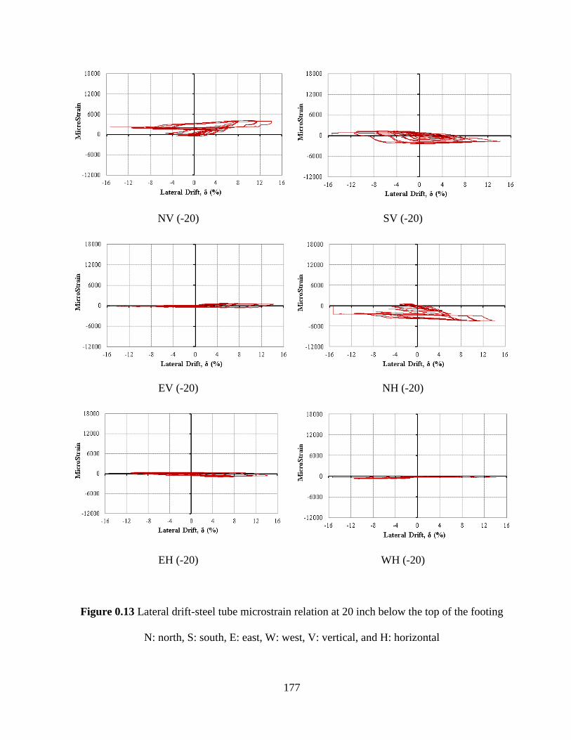
177

NV (-20) SV (-20)

EV (-20) NH (-20)

EH (-20) WH (-20)



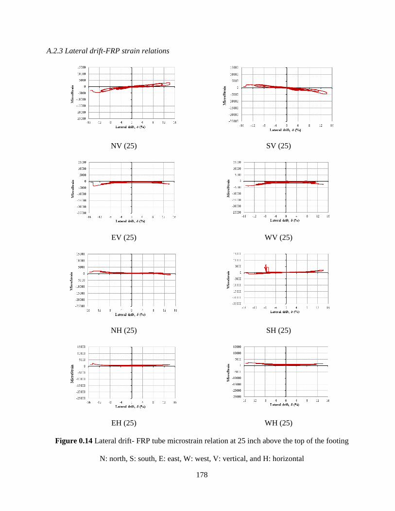
178

A.2.3 Lateral drift-FRP strain relations

NV (25) SV (25)

EV (25) WV (25)

NH (25) SH (25)

EH (25) WH (25)

Figure 0.14 Lateral drift- FRP tube microstrain relation at 25 inch above the top of the footing


179

NV (20) SV (20)

EV (20) WV (20)

NH (20) SH (20)

EH (20) WH (20)



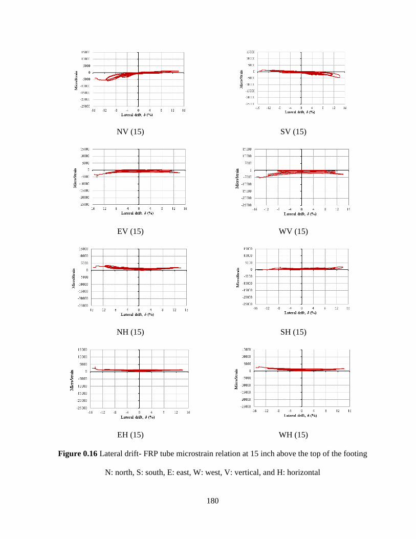
180

NV (15) SV (15)

EV (15) WV (15)

NH (15) SH (15)

EH (15) WH (15)



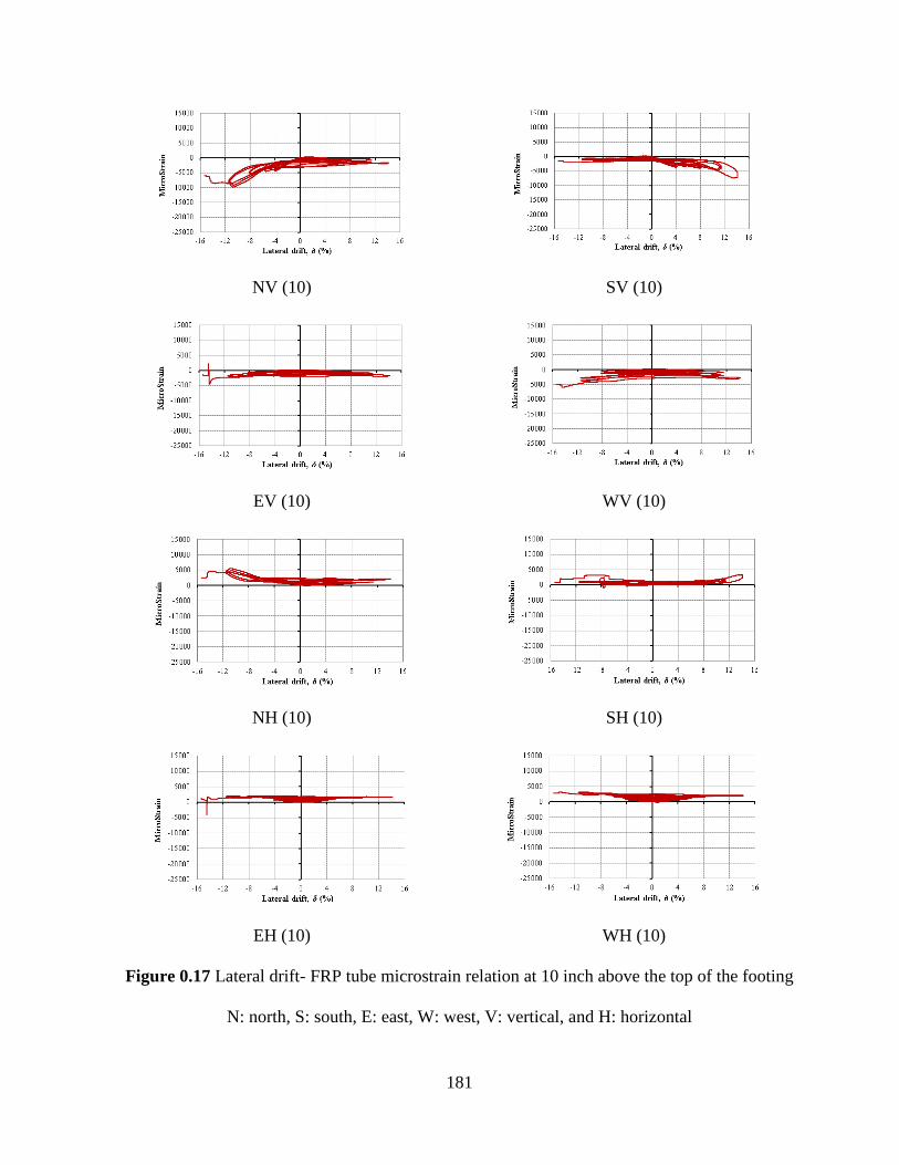
181

NV (10) SV (10)

EV (10) WV (10)

NH (10) SH (10)

EH (10) WH (10)



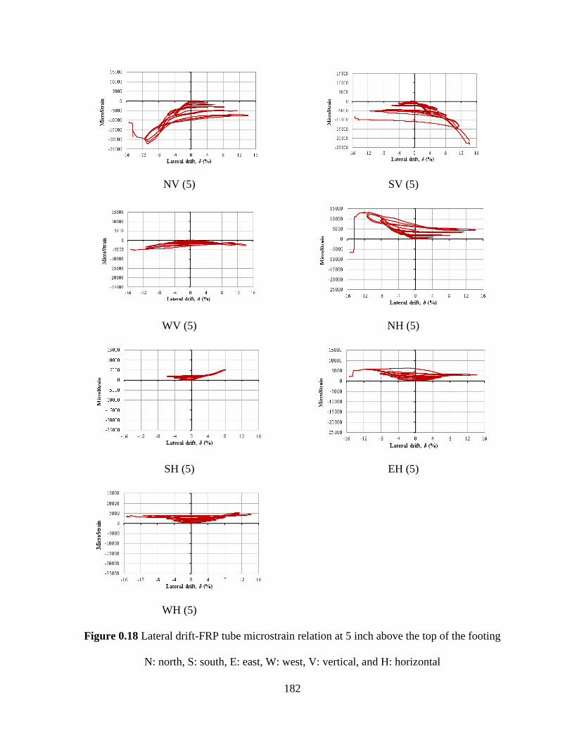
182

NV (5) SV (5)

WV (5) NH (5)

SH (5) EH (5)

WH (5)

Figure 0.18 Lateral drift-FRP tube microstrain relation at 5 inch above the top of the footing


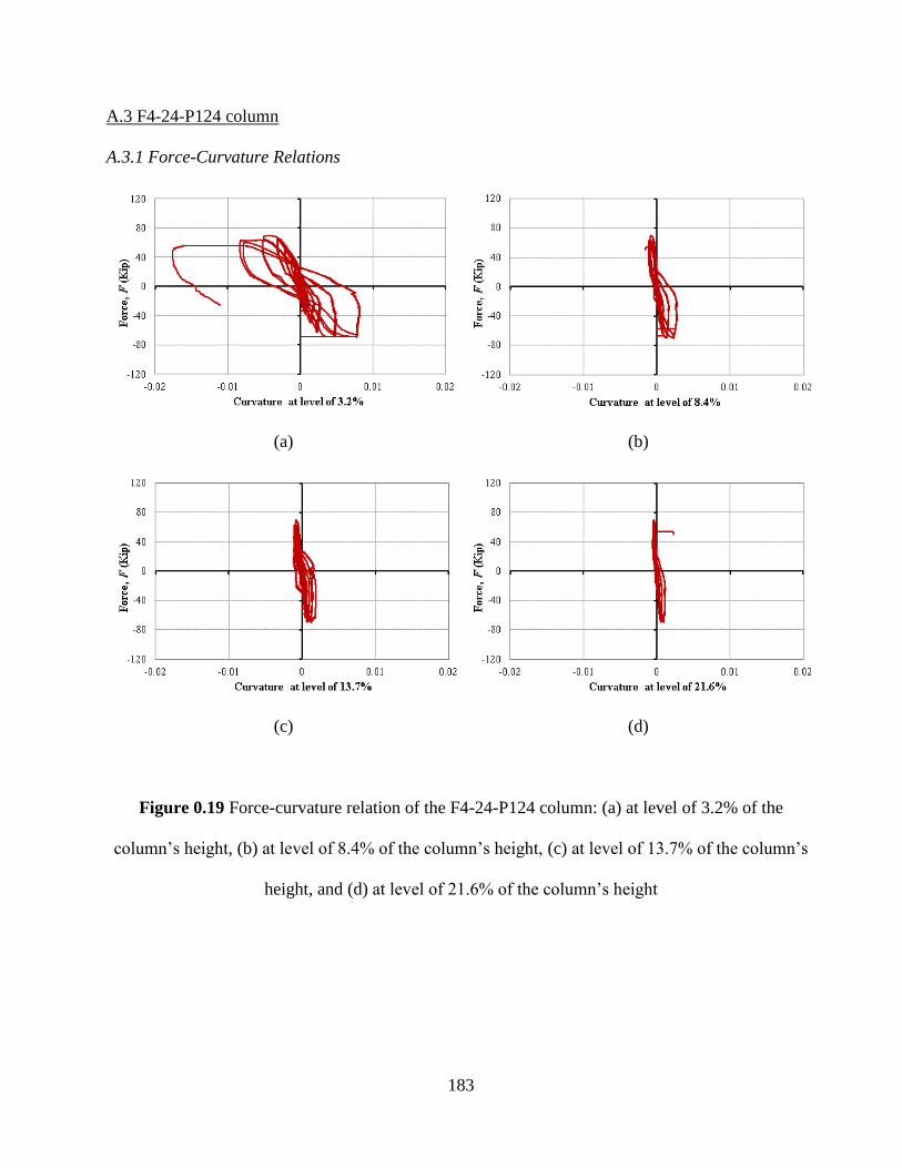
183

A.3 F4-24-P124 column


(a) (b)

(c) (d)

Figure 0.19 Force-curvature relation of the F4-24-P124 column: (a) at level of 3.2% of the


height, and (d) at level of 21.6% of the column’s height

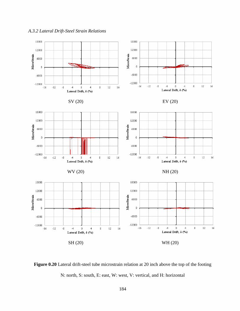
184


SV (20) EV (20)

WV (20) NH (20)

SH (20) WH (20)



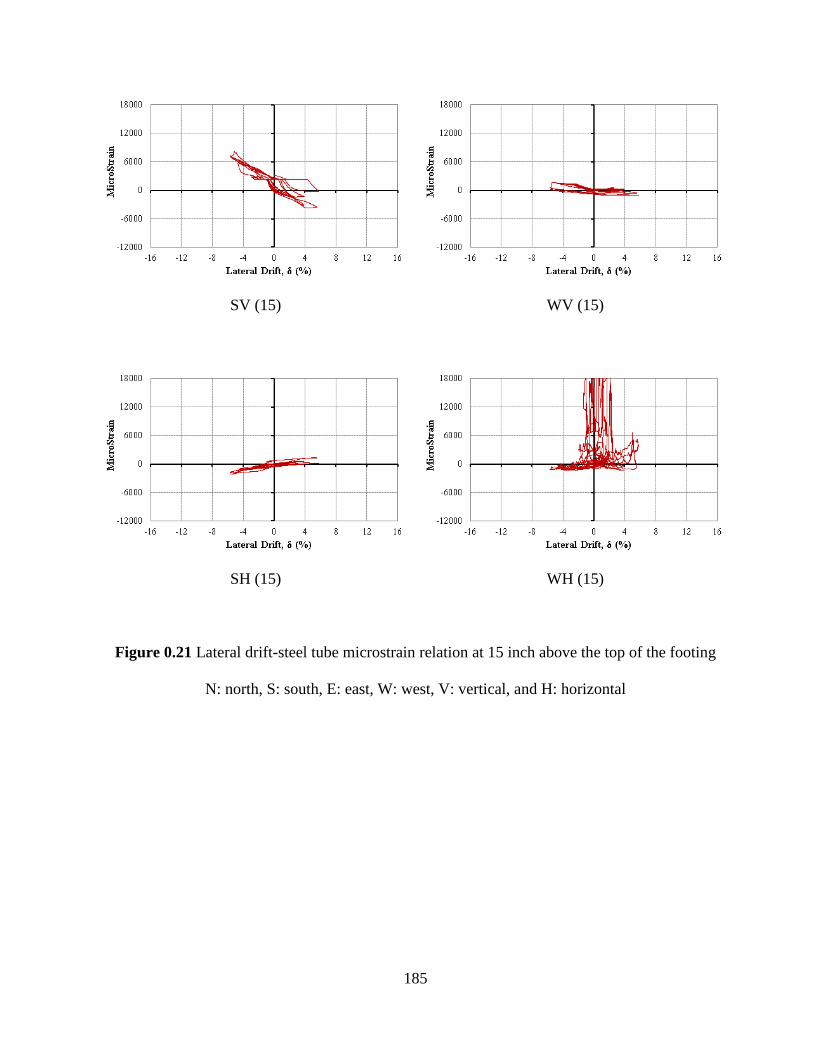
185

SV (15) WV (15)

SH (15) WH (15)



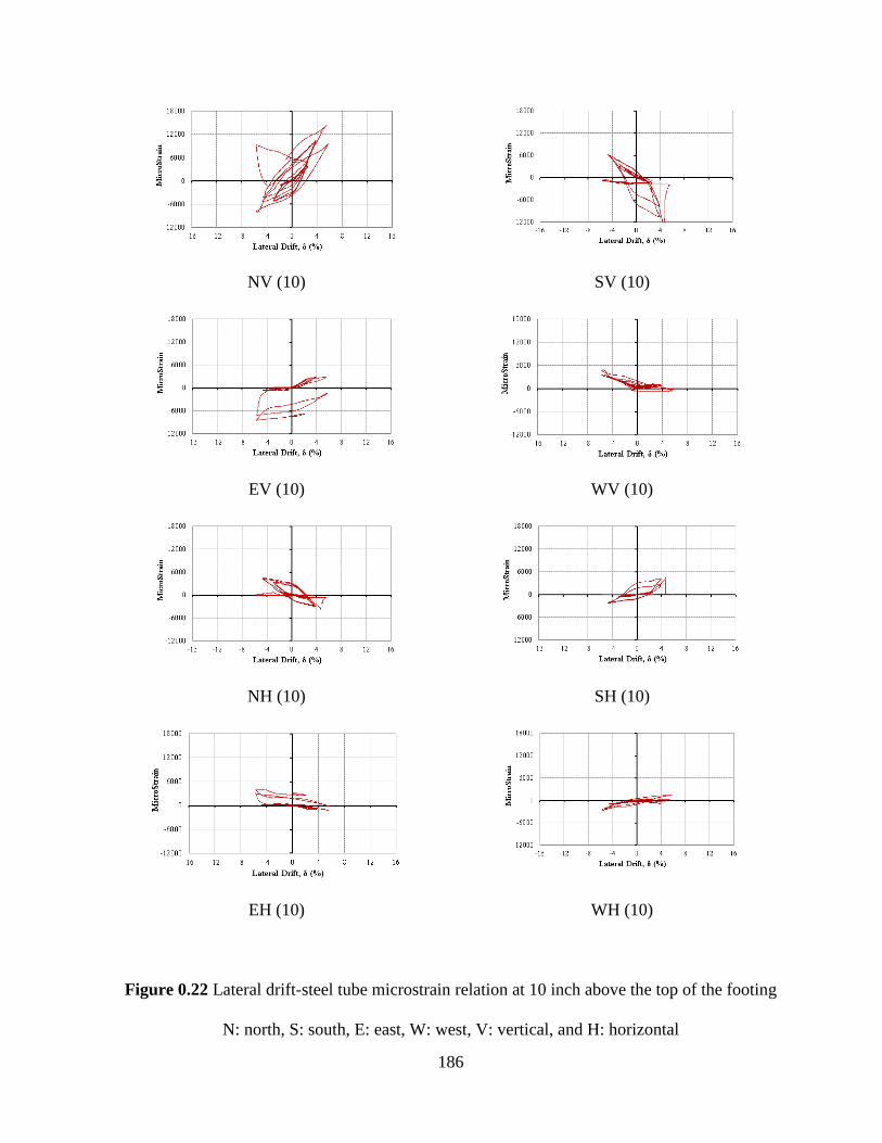
186

NV (10) SV (10)

EV (10) WV (10)

NH (10) SH (10)

EH (10) WH (10)



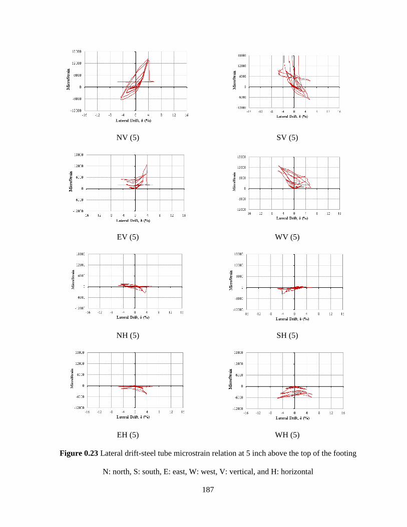
187

NV (5) SV (5)

EV (5) WV (5)

NH (5) SH (5)

EH (5) WH (5)



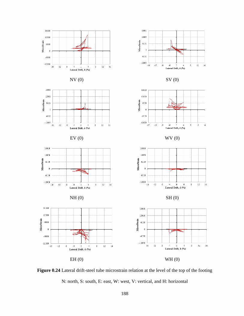
188

NV (0) SV (0)

EV (0) WV (0)

NH (0) SH (0)

EH (0) WH (0)



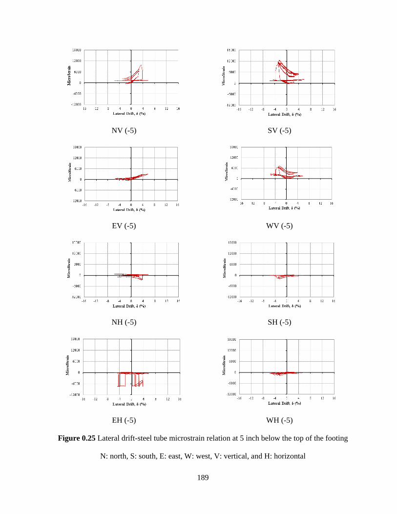
189

NV (-5) SV (-5)

EV (-5) WV (-5)

NH (-5) SH (-5)

EH (-5) WH (-5)



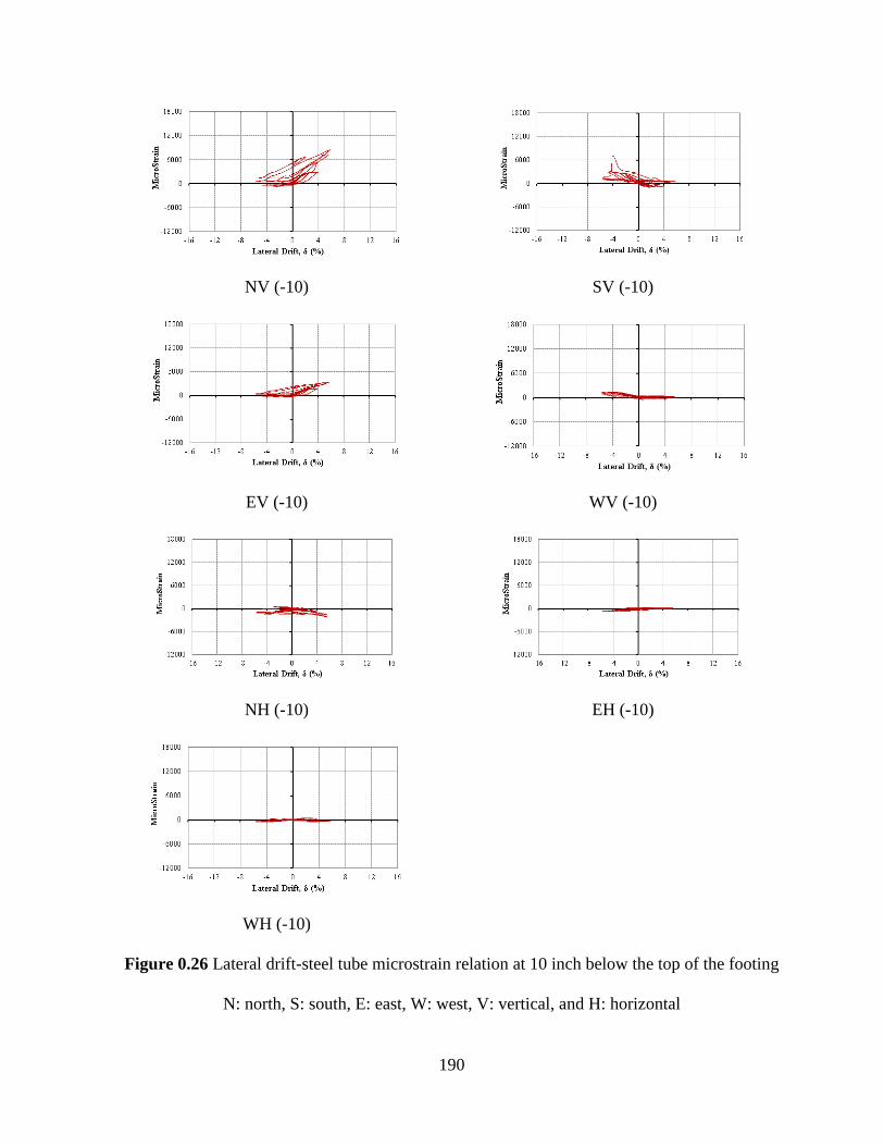
190

NV (-10) SV (-10)

EV (-10) WV (-10)

NH (-10) EH (-10)

WH (-10)



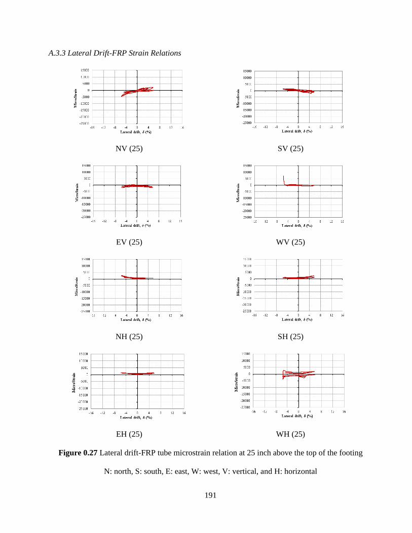
191

A.3.3 Lateral Drift-FRP Strain Relations

NV (25) SV (25)

EV (25) WV (25)

NH (25) SH (25)

EH (25) WH (25)



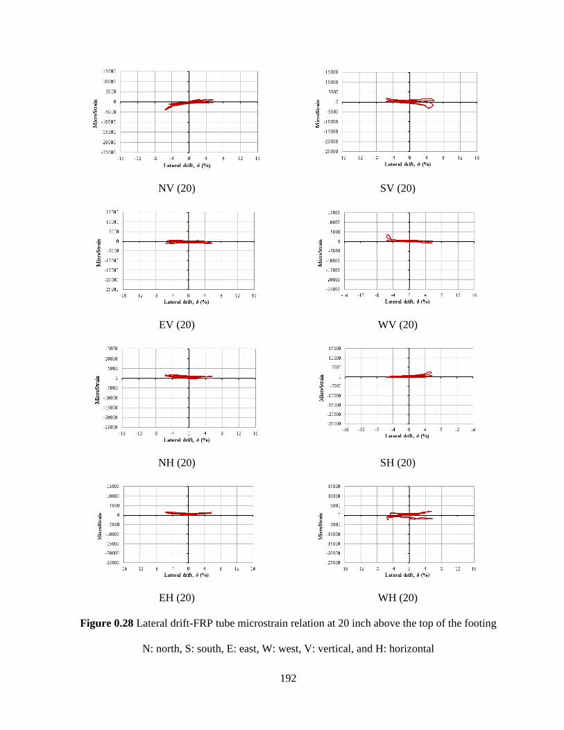
192

NV (20) SV (20)

EV (20) WV (20)

NH (20) SH (20)

EH (20) WH (20)



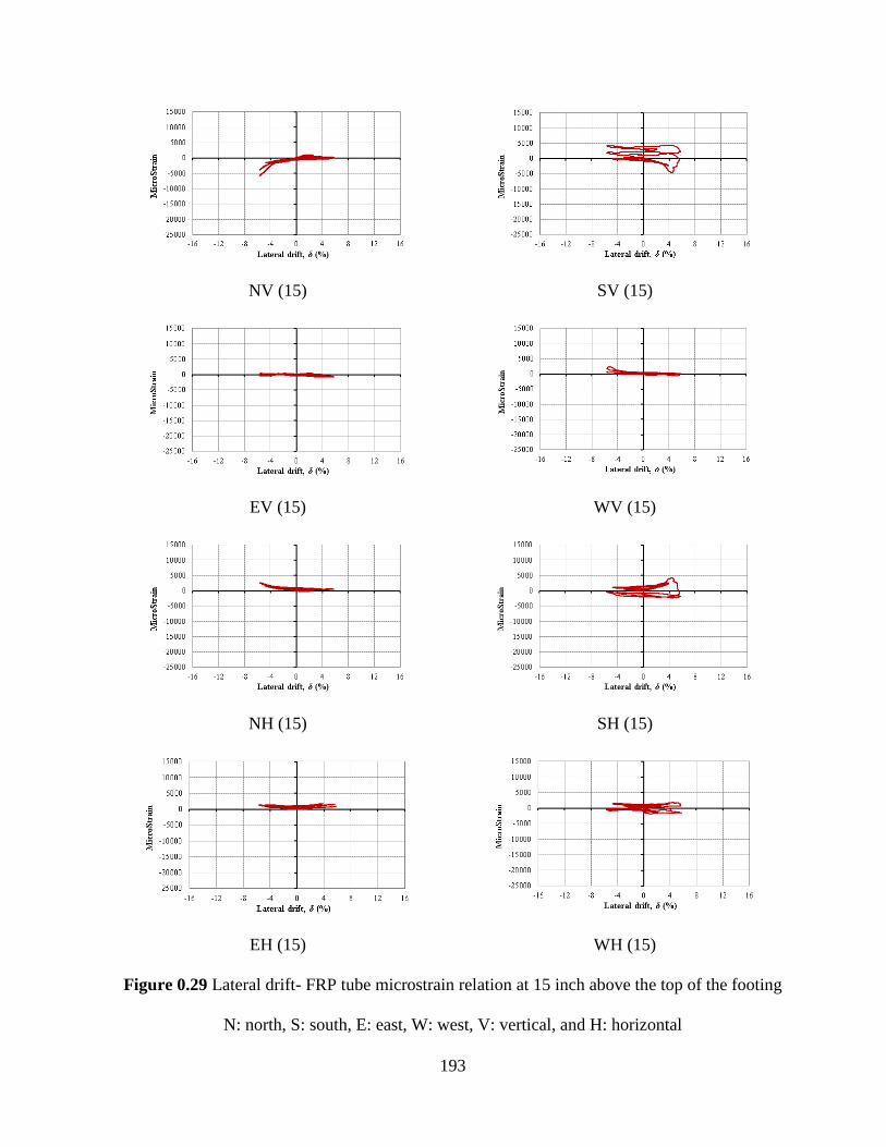
193

NV (15) SV (15)

EV (15) WV (15)

NH (15) SH (15)

EH (15) WH (15)



194

NV (10) SV (10)

EV (10) NH (10)

SH (10) EH (10)



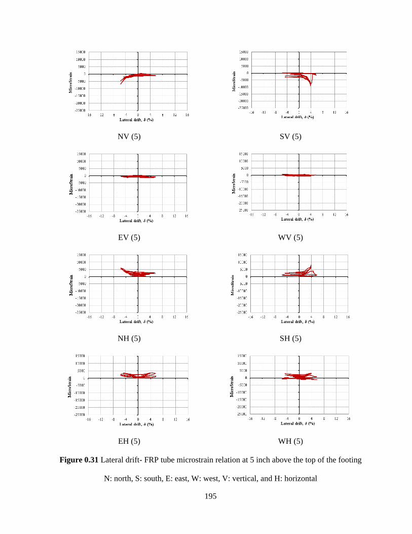
195

NV (5) SV (5)

EV (5) WV (5)

NH (5) SH (5)

EH (5) WH (5)



196

SV (0) EV (0)

WV (0) NH (0)

SH (0) EH (0)

WH (0)

Figure 0.32 Lateral drift- FRP tube microstrain relation at the top of the footing

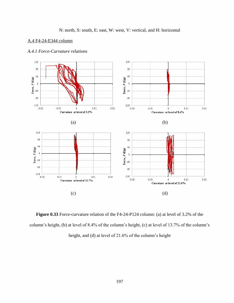
197


A.4 F4-24-E344 column

A.4.1 Force-Curvature relations

(a) (b)

(c) (d)

Figure 0.33 Force-curvature relation of the F4-24-P124 column: (a) at level of 3.2% of the


height, and (d) at level of 21.6% of the column’s height

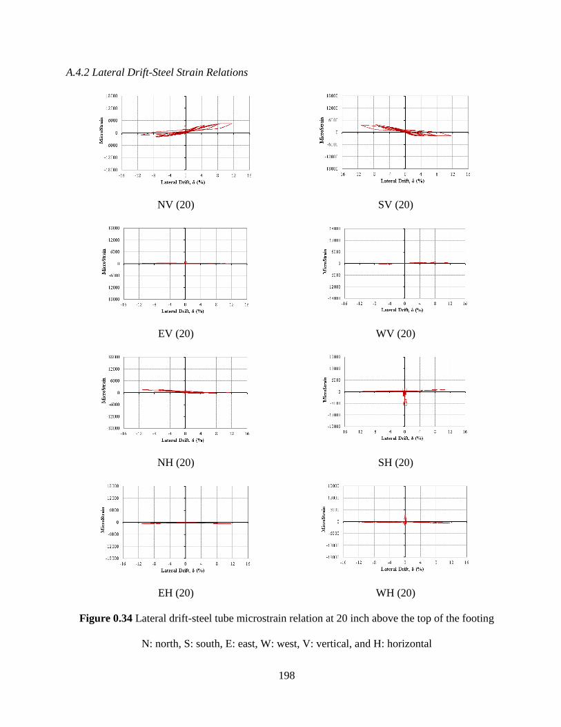
198


NV (20) SV (20)

EV (20) WV (20)

NH (20) SH (20)

EH (20) WH (20)



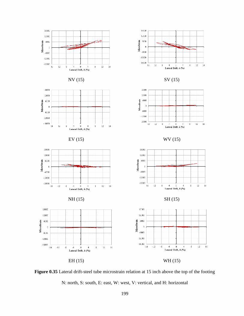
199

NV (15) SV (15)

EV (15) WV (15)

NH (15) SH (15)

EH (15) WH (15)



200

NV (10) SV (10)

EV (10) WV (10)

NH (10) SH (10)

WH (10)



201

NV (5) SV (5)

EV (5) WV (5)

NH (5) SH (5)

EH (5) WH (5)



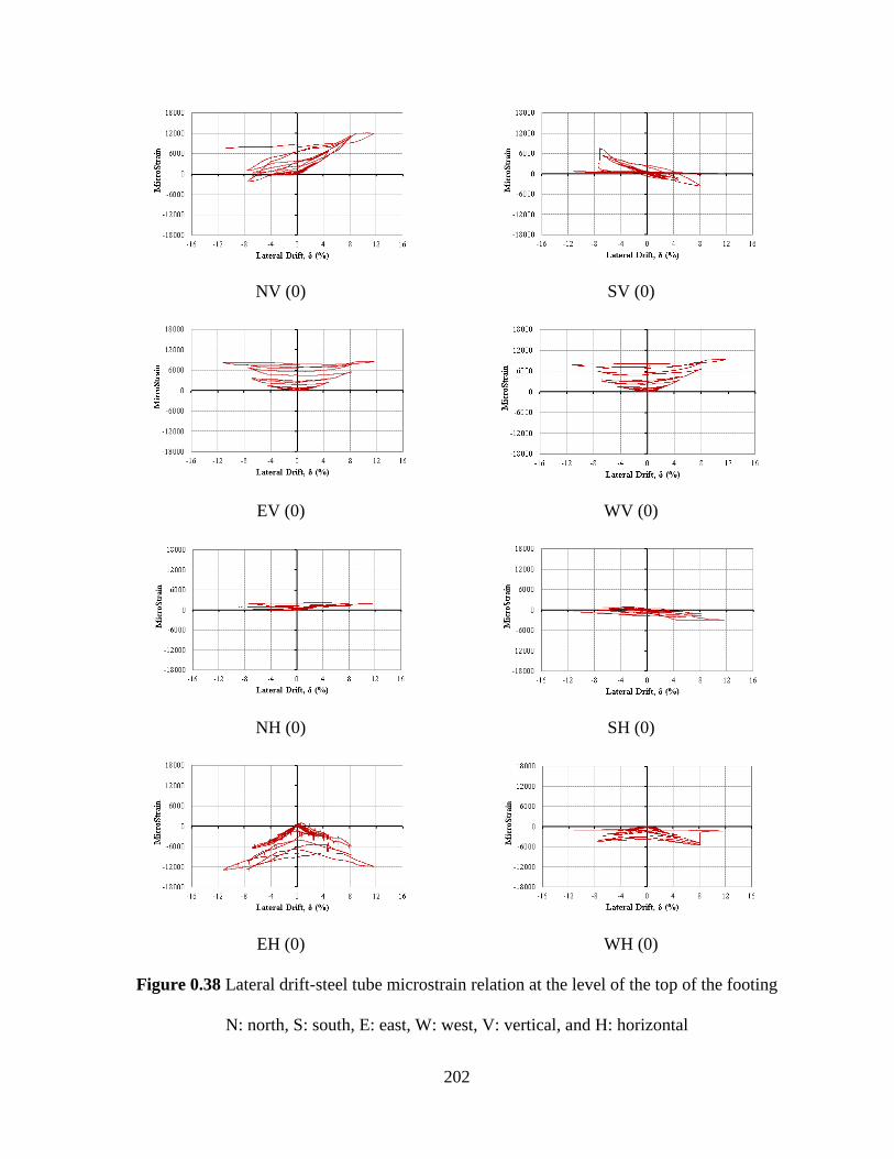
202

NV (0) SV (0)

EV (0) WV (0)

NH (0) SH (0)

EH (0) WH (0)



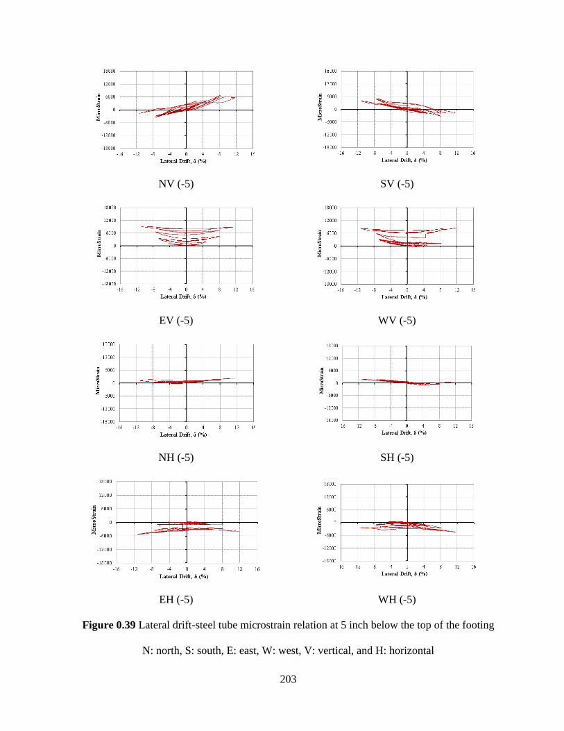
203

NV (-5) SV (-5)

EV (-5) WV (-5)

NH (-5) SH (-5)

EH (-5) WH (-5)



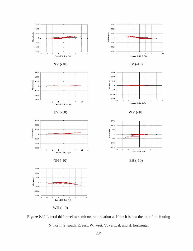
204

NV (-10) SV (-10)

EV (-10) WV (-10)

NH (-10) EH (-10)

WH (-10)



205

A.4.3 Lateral Drift-FRP Strain Relations

NV (25) SV (25)

EV (25) WV (25)

NH (25) SH (25)

EH (25) WH (25)



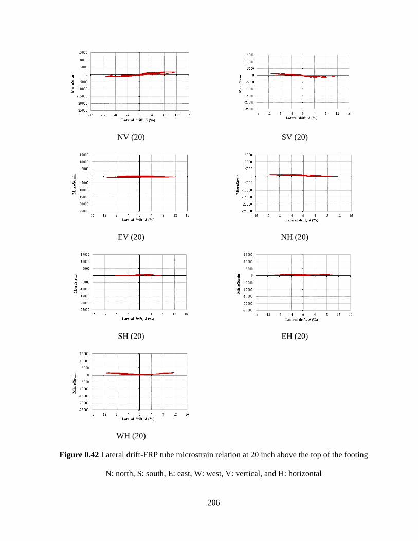
206

NV (20) SV (20)

EV (20) NH (20)

SH (20) EH (20)

WH (20)



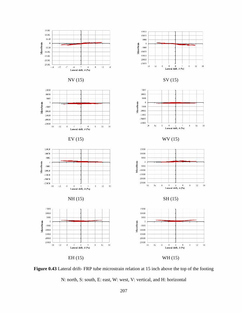
207

NV (15) SV (15)

EV (15) WV (15)

NH (15) SH (15)

EH (15) WH (15)



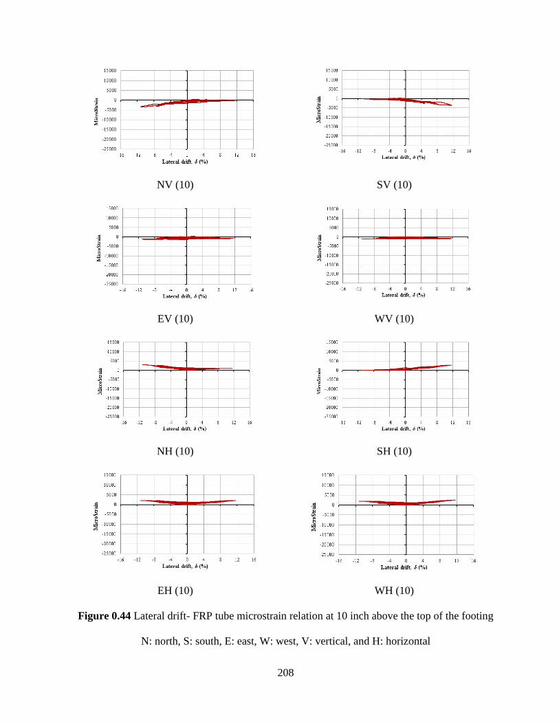
208

NV (10) SV (10)

EV (10) WV (10)

NH (10) SH (10)

EH (10) WH (10)



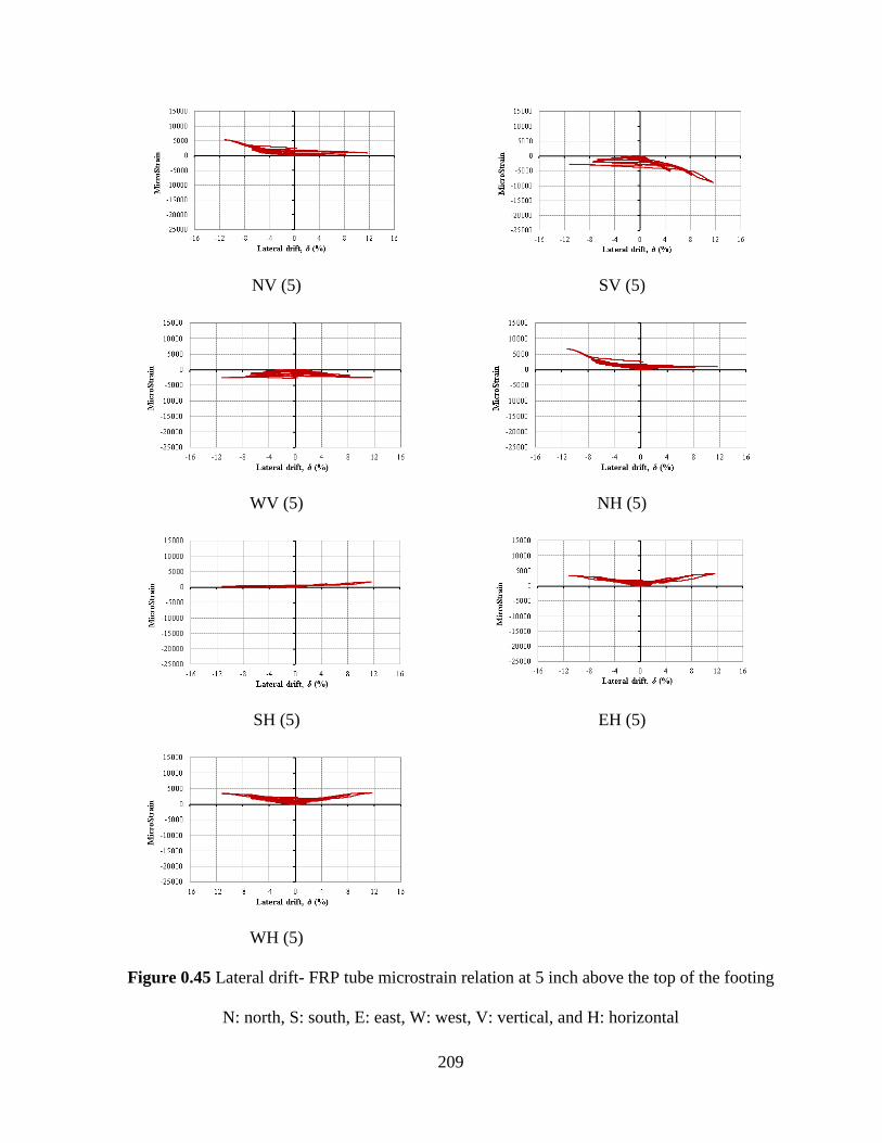
209

NV (5) SV (5)

WV (5) NH (5)

SH (5) EH (5)

WH (5)



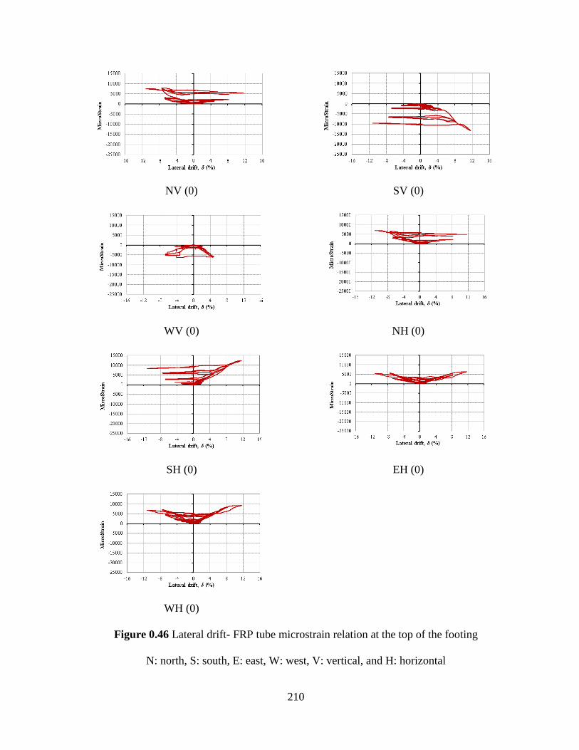
210

NV (0) SV (0)

WV (0) NH (0)

SH (0) EH (0)

WH (0)

Figure 0.46 Lateral drift- FRP tube microstrain relation at the top of the footing


Report # MATC-MS&T: 297 Final Report · v 7.5.5 Strain Rate Effect.....143 Chapter 8 Comparisons...

Documents

Transcript of Report # MATC-MS&T: 297 Final Report · v 7.5.5 Strain Rate Effect.....143 Chapter 8 Comparisons...